Download A USER GUIDE FOR DRAGON VERSION4 G. Marleau, A. Hébert

TECHNICAL REPORT
IGE–294
A USER GUIDE FOR DRAGON VERSION4
G. Marleau, A. H´
ebert and R. Roy
Institut de g´enie nucl´eaire
D´epartement de g´enie m´ecanique
´
Ecole
Polytechnique de Montr´eal
September 22, 2015
IGE–294
ii
Copyright Notice for DRAGON
The development of DRAGON is financially supported, directly or indirectly, by various organiza´
tions including Ecole
Polytechnique de Montr´eal, Hydro–Qu´ebec and the Hydro–Qu´ebec chair in nuclear
engineering, the Natural Science and Engineering Research Council of Canada (NSERC), Atomic Energy
of Canada limited (AECL) and the CANDU Owners Group (COG). The code DRAGON and its users
´
guide are and will remain the property of Ecole
Polytechnique de Montr´eal. The PostScript utility module
used in DRAGON is based on PSPLOT which is owned by Kevin E. Kohler at the Nova Southeastern
University Oceanographic Center in Florida.
Dragon is free software; you can redistribute it and/or modify it under the terms of the GNU Lesser
General Public License as published by the Free Software Foundation; either version 2.1 of the License,
or (at your option) any later version.
´
Permission is granted to the public to copy DRAGON without charge. Ecole
Polytechnique de
Montr´eal, makes no warranty, express or implied, and assumes no liability or responsibility for the use of
DRAGON.
IGE–294
iii
Acknowledgments
´
The computer code DRAGON results from a concerted effort made at Ecole
Polytechnique de Montr´eal.
´
The main authors of this report would therefore like to express their thanks to Ecole
Polytechnique de
Montr´eal for its support along the years as well as to the graduate students and research associates which
have contributed to the development of DRAGON along the years. We would also like to thank Kevin
E. Kohler at the Nova Southeastern University Oceanographic Center for letting us use and distribute a
PostScript utility module derived from his PSPLOT package. Finally, the DRAGON team would never
have survived without the financial support of the Natural Science and Engineering Research Council of
Canada (NSERC), Hydro–Qu´ebec, Atomic Energy of Canada limited (AECL) and the CANDU Owners
Group (COG).
IGE–294
iv
SUMMARY
The computer code DRAGON contains a collection of models which can simulate the neutronic behaviour of a unit cell or a fuel assembly in a nuclear reactor. It includes all of the functions that
characterize a lattice cell code, namely: the interpolation of microscopic cross sections which are supplied by means of standard libraries; resonance self-shielding calculations in multidimensional geometries;
multigroup and multidimensional neutron flux calculations which can take into account neutron leakage;
transport-transport or transport-diffusion equivalence calculations as well as editing of condensed and
homogenized nuclear properties for reactor calculations; and finally isotopic depletion calculations.
The code DRAGON contains a multigroup iterator conceived to control a number of different algorithms for the solution of the neutron transport equation. Each of these algorithms is presented in the
form of a one-group solution procedure where the contributions from other energy groups are included in a
source term. The current version of DRAGON contains many such algorithms. The SYBIL option which
solves the integral transport equation using the collision probability method for simple one-dimensional
(1–D) geometries (either plane, cylindrical or spherical) and the interface current method for 2–D Cartesian or hexagonal assemblies. The EXCELL option which solves the integral transport equation using the
collision probability method for general 2–D geometries and for three-dimensional (3–D) assemblies. The
MCCG option solves the integro-differential transport equation using the long characteristics method for
general 2–D and 3–D geometries.
The execution of DRAGON is controlled by the generalized GAN driver. It is modular and can be
interfaced easily with other production codes.
IGE–294
v
Contents
Copyright Notice for DRAGON . . . . . . . . . . . . . . . . . .
Acknowledgments . . . . . . . . . . . . . . . . . . . . . . . . . .
Contents . . . . . . . . . . . . . . . . . . . . . . . . . . . . . . .
List of Figures . . . . . . . . . . . . . . . . . . . . . . . . . . . .
List of Tables . . . . . . . . . . . . . . . . . . . . . . . . . . . .
1
INTRODUCTION . . . . . . . . . . . . . . . . . . . . . . .
2
GENERAL STRUCTURE OF THE DRAGON INPUT . .
2.1
Data organization . . . . . . . . . . . . . . . . . . .
2.2
DRAGON Data Structure and Module Declarations
2.3
The DRAGON Modules . . . . . . . . . . . . . . . .
2.4
The Utility Modules . . . . . . . . . . . . . . . . . .
2.5
The DRAGON Data Structures . . . . . . . . . . . .
2.6
Main Updates in DRAGON . . . . . . . . . . . . . .
3
THE DRAGON MODULES . . . . . . . . . . . . . . . . .
3.1
The MAC: module . . . . . . . . . . . . . . . . . . . .
3.1.1
Input structure for module MAC: . . . . . .
3.1.2
Macroscopic cross section definition . . . .
3.1.3
Update structure for operator MAC: . . . .
3.2
The LIB: module . . . . . . . . . . . . . . . . . . . .
3.2.1
Data input for module LIB: . . . . . . . .
3.2.2
Depletion data structure . . . . . . . . . .
3.2.3
Mixture description structure . . . . . . . .
3.3
The GEO: module . . . . . . . . . . . . . . . . . . . .
3.3.1
Data input for module GEO: . . . . . . . .
3.3.2
Boundary conditions . . . . . . . . . . . . .
3.3.3
Spatial properties of geometry . . . . . . .
3.3.4
Physical properties of geometry . . . . . .
3.3.5
Double-heterogeneity . . . . . . . . . . . .
3.3.6
Do-it-yourself geometries . . . . . . . . . .
3.4
The tracking modules . . . . . . . . . . . . . . . . .
3.4.1
The SYBILT: tracking module . . . . . . .
3.4.2
The EXCELT: tracking module . . . . . . .
3.4.3
The NXT: tracking module . . . . . . . . .
3.4.4
The MCCGT: tracking module . . . . . . . .
3.4.5
The SNT: tracking module . . . . . . . . .
3.4.6
The BIVACT: tracking module . . . . . . .
3.4.7
The TRIVAT: tracking module . . . . . . .
3.5
The SHI: module . . . . . . . . . . . . . . . . . . . .
3.5.1
Data input for module SHI: . . . . . . . .
3.6
The USS: module . . . . . . . . . . . . . . . . . . . .
3.6.1
Data input for module USS: . . . . . . . .
3.7
The ASM: module . . . . . . . . . . . . . . . . . . . .
3.7.1
Data input for module ASM: . . . . . . . .
3.8
The FLU: module . . . . . . . . . . . . . . . . . . . .
3.8.1
Data input for module FLU: . . . . . . . .
3.8.2
Leakage model specification structure . . .
3.9
The EDI: module . . . . . . . . . . . . . . . . . . . .
3.9.1
Data input for module EDI: . . . . . . . .
3.9.2
Homogenization and condensation with the
3.9.3
Homogenization and condensation with the
3.10 The EVO: module . . . . . . . . . . . . . . . . . . . .
3.10.1
Data input for module EVO: . . . . . . . .
3.10.2
Power normalization in EVO: . . . . . . . .
. . . . .
. . . . .
. . . . .
. . . . .
. . . . .
. . . . .
. . . . .
. . . . .
. . . . .
. . . . .
. . . . .
. . . . .
. . . . .
. . . . .
. . . . .
. . . . .
. . . . .
. . . . .
. . . . .
. . . . .
. . . . .
. . . . .
. . . . .
. . . . .
. . . . .
. . . . .
. . . . .
. . . . .
. . . . .
. . . . .
. . . . .
. . . . .
. . . . .
. . . . .
. . . . .
. . . . .
. . . . .
. . . . .
. . . . .
. . . . .
. . . . .
. . . . .
. . . . .
. . . . .
. . . . .
. . . . .
. . . . .
. . . . .
flux . .
flux and
. . . . .
. . . . .
. . . . .
. . . . . . .
. . . . . . .
. . . . . . .
. . . . . . .
. . . . . . .
. . . . . . .
. . . . . . .
. . . . . . .
. . . . . . .
. . . . . . .
. . . . . . .
. . . . . . .
. . . . . . .
. . . . . . .
. . . . . . .
. . . . . . .
. . . . . . .
. . . . . . .
. . . . . . .
. . . . . . .
. . . . . . .
. . . . . . .
. . . . . . .
. . . . . . .
. . . . . . .
. . . . . . .
. . . . . . .
. . . . . . .
. . . . . . .
. . . . . . .
. . . . . . .
. . . . . . .
. . . . . . .
. . . . . . .
. . . . . . .
. . . . . . .
. . . . . . .
. . . . . . .
. . . . . . .
. . . . . . .
. . . . . . .
. . . . . . .
. . . . . . .
. . . . . . .
. . . . . . .
. . . . . . .
. . . . . . .
. . . . . . .
. . . . . . .
adjoint flux
. . . . . . .
. . . . . . .
. . . . . . .
.
.
.
.
.
.
.
.
.
.
.
.
.
.
.
.
.
.
.
.
.
.
.
.
.
.
.
.
.
.
.
.
.
.
.
.
.
.
.
.
.
.
.
.
.
.
.
.
.
.
.
.
.
.
.
.
.
.
.
.
.
.
.
.
.
.
.
.
.
.
.
.
.
.
.
.
.
.
.
.
.
.
.
.
.
.
.
.
.
.
.
.
.
.
.
.
.
.
.
.
.
.
.
.
.
.
.
.
.
.
.
.
.
.
.
.
.
.
.
.
.
.
.
.
.
.
.
.
.
.
.
.
.
.
.
.
.
.
.
.
.
.
.
.
.
.
.
.
.
.
.
.
.
.
.
.
.
.
.
.
.
.
.
.
.
.
.
.
.
.
.
.
.
.
.
.
.
.
.
.
.
.
.
.
.
.
.
.
.
.
.
.
.
.
.
.
.
.
.
.
.
.
.
.
.
.
.
.
.
.
.
.
.
.
.
.
.
.
.
.
.
.
.
.
.
.
.
.
.
.
.
.
.
.
.
.
.
.
.
.
.
.
.
.
.
.
.
.
.
.
.
.
.
.
.
.
.
.
.
.
.
.
.
.
.
ii
iii
v
viii
ix
1
2
2
3
4
6
6
7
9
9
10
12
14
16
16
22
23
29
29
32
41
46
56
56
58
60
63
67
71
74
76
79
82
82
84
85
88
88
91
92
93
97
97
103
103
105
107
111
IGE–294
3.11
4
5
6
The SPH: module . . . . . . . . . . . . . . . . . . . . . . . . . .
3.11.1
Data input for module SPH: . . . . . . . . . . . . . .
3.11.2
Data input for module SPH: . . . . . . . . . . . . . .
3.12 The CFC: module . . . . . . . . . . . . . . . . . . . . . . . . . .
3.12.1
Data input for module CFC: . . . . . . . . . . . . . .
3.13 The INFO: module . . . . . . . . . . . . . . . . . . . . . . . . .
3.13.1
Data input for module INFO: . . . . . . . . . . . . . .
3.14 The COMPO: module . . . . . . . . . . . . . . . . . . . . . . . .
3.14.1
Initialization data input for module COMPO: . . . . . .
3.14.2
Modification data input for module COMPO: . . . . . .
3.14.3
Modification (catenate) data input for module COMPO:
3.14.4
Display data input for module COMPO: . . . . . . . . .
3.15 The TLM: module . . . . . . . . . . . . . . . . . . . . . . . . . .
3.15.1
Data input for module TLM: . . . . . . . . . . . . . .
3.16 The M2T: module . . . . . . . . . . . . . . . . . . . . . . . . . .
3.16.1
Data input for module M2T: . . . . . . . . . . . . . .
3.17 The CHAB: module . . . . . . . . . . . . . . . . . . . . . . . . .
3.17.1
Data input for module CHAB: . . . . . . . . . . . . . .
3.18 The CPO: module . . . . . . . . . . . . . . . . . . . . . . . . . .
3.18.1
Data input for module CPO: . . . . . . . . . . . . . .
3.19 The SAP: module . . . . . . . . . . . . . . . . . . . . . . . . . .
3.19.1
Initialization data input for module SAP: . . . . . . .
3.19.2
Modification data input for module SAP: . . . . . . .
3.19.3
Modification (catenate) data input for module SAP: .
3.20 The MC: module . . . . . . . . . . . . . . . . . . . . . . . . . .
3.20.1
Data input for module MC: . . . . . . . . . . . . . . .
3.21 The T: module . . . . . . . . . . . . . . . . . . . . . . . . . . .
3.22 The DMAC: module . . . . . . . . . . . . . . . . . . . . . . . . .
3.22.1
Data input for module DMAC: . . . . . . . . . . . . . .
3.23 The DREF: module . . . . . . . . . . . . . . . . . . . . . . . . .
3.24 The SENS: module . . . . . . . . . . . . . . . . . . . . . . . . .
3.24.1
Data input for module SENS: . . . . . . . . . . . . . .
3.25 The DUO: module . . . . . . . . . . . . . . . . . . . . . . . . . .
3.25.1
Data input for module DUO: . . . . . . . . . . . . . .
3.25.2
Theory . . . . . . . . . . . . . . . . . . . . . . . . . .
3.26 The PSP: module . . . . . . . . . . . . . . . . . . . . . . . . .
3.26.1
Data input for module PSP: . . . . . . . . . . . . . .
THE UTILITY MODULES . . . . . . . . . . . . . . . . . . . . . . . .
4.1
The equality module . . . . . . . . . . . . . . . . . . . . . . . .
4.2
The UTL: module . . . . . . . . . . . . . . . . . . . . . . . . .
4.3
The DELETE: module . . . . . . . . . . . . . . . . . . . . . . .
4.4
The BACKUP: module . . . . . . . . . . . . . . . . . . . . . .
4.5
The RECOVER: module . . . . . . . . . . . . . . . . . . . . .
4.6
The ADD: module . . . . . . . . . . . . . . . . . . . . . . . . .
4.7
The MPX: module . . . . . . . . . . . . . . . . . . . . . . . . .
4.8
The STAT: module . . . . . . . . . . . . . . . . . . . . . . . . .
4.9
The GREP: module . . . . . . . . . . . . . . . . . . . . . . . .
4.10 The MSTR module . . . . . . . . . . . . . . . . . . . . . . . . .
4.11 The FIND0: module . . . . . . . . . . . . . . . . . . . . . . . .
4.12 The ABORT: module . . . . . . . . . . . . . . . . . . . . . . .
4.13 The END: module . . . . . . . . . . . . . . . . . . . . . . . . .
THE MPI MODULES . . . . . . . . . . . . . . . . . . . . . . . . . . .
5.1
The DRVMPI: module . . . . . . . . . . . . . . . . . . . . . . .
5.2
The SNDMPI: module . . . . . . . . . . . . . . . . . . . . . . .
EXAMPLES . . . . . . . . . . . . . . . . . . . . . . . . . . . . . . . .
vi
.
.
.
.
.
.
.
.
.
.
.
.
.
.
.
.
.
.
.
.
.
.
.
.
.
.
.
.
.
.
.
.
.
.
.
.
.
.
.
.
.
.
.
.
.
.
.
.
.
.
.
.
.
.
.
.
.
.
.
.
.
.
.
.
.
.
.
.
.
.
.
.
.
.
.
.
.
.
.
.
.
.
.
.
.
.
.
.
.
.
.
.
.
.
.
.
.
.
.
.
.
.
.
.
.
.
.
.
.
.
.
.
.
.
.
.
.
.
.
.
.
.
.
.
.
.
.
.
.
.
.
.
.
.
.
.
.
.
.
.
.
.
.
.
.
.
.
.
.
.
.
.
.
.
.
.
.
.
.
.
.
.
.
.
.
.
.
.
.
.
.
.
.
.
.
.
.
.
.
.
.
.
.
.
.
.
.
.
.
.
.
.
.
.
.
.
.
.
.
.
.
.
.
.
.
.
.
.
.
.
.
.
.
.
.
.
.
.
.
.
.
.
.
.
.
.
.
.
.
.
.
.
.
.
.
.
.
.
.
.
.
.
.
.
.
.
.
.
.
.
.
.
.
.
.
.
.
.
.
.
.
.
.
.
.
.
.
.
.
.
.
.
.
.
.
.
.
.
.
.
.
.
.
.
.
.
.
.
.
.
.
.
.
.
.
.
.
.
.
.
.
.
.
.
.
.
.
.
.
.
.
.
.
.
.
.
.
.
.
.
.
.
.
.
.
.
.
.
.
.
.
.
.
.
.
.
.
.
.
.
.
.
.
.
.
.
.
.
.
.
.
.
.
.
.
.
.
.
.
.
.
.
.
.
.
.
.
.
.
.
.
.
.
.
.
.
.
.
.
.
.
.
.
.
.
.
.
.
.
.
.
.
.
.
.
.
.
.
.
.
.
.
.
.
.
.
.
.
.
.
.
.
.
.
.
.
.
.
.
.
.
.
.
.
.
.
.
.
.
.
.
.
.
.
.
.
.
.
.
.
.
.
.
.
.
.
.
.
.
.
.
.
.
.
.
.
.
.
.
.
.
.
.
.
.
.
.
.
.
.
.
.
.
.
.
.
.
.
.
.
.
.
.
.
.
.
.
.
.
.
.
.
.
.
.
.
.
.
.
.
.
.
.
.
.
.
.
.
.
.
.
.
.
.
.
.
.
.
.
.
.
.
.
.
.
.
.
.
.
.
.
.
.
.
.
.
.
.
.
.
.
.
.
.
.
.
.
.
.
.
.
.
.
.
.
.
.
.
.
.
.
.
.
.
.
.
.
.
.
.
.
.
.
.
.
.
.
.
.
.
.
.
.
.
.
.
.
.
.
.
.
.
.
.
.
.
.
.
.
.
.
.
.
.
.
112
113
114
118
119
121
121
124
126
129
130
130
132
132
135
135
137
137
139
139
141
143
145
146
148
148
150
151
151
153
155
155
157
157
158
160
160
162
162
163
165
166
167
168
169
170
171
173
175
176
177
178
178
179
180
IGE–294
6.1
6.2
6.3
Scattering cross sections . . . . . . . . . . . . . . . . . . . . . . . . . . . . . . . . .
Geometries . . . . . . . . . . . . . . . . . . . . . . . . . . . . . . . . . . . . . . . .
MATXS7A microscopic cross-section examples . . . . . . . . . . . . . . . . . . . .
6.3.1
(TCXA01) – The Mosteller benchmark. . . . . . . . . . . . . . . . . . . .
6.4
Macroscopic cross sections examples . . . . . . . . . . . . . . . . . . . . . . . . . .
6.4.1
(TCM01) – Annular region . . . . . . . . . . . . . . . . . . . . . . . . . .
6.4.2
(TCM02) – The Stankovski test case. . . . . . . . . . . . . . . . . . . . .
6.4.3
(TCM03) – Watanabe and Maynard problem with a void region. . . . . .
6.4.4
(TCM04) – Adjuster rod in a CANDU type supercell. . . . . . . . . . . .
6.4.5
(TCM05) – Comparison of leakage models . . . . . . . . . . . . . . . . .
6.4.6
(TCM06) – Buckling search without fission source . . . . . . . . . . . . .
6.4.7
(TCM07) – Test of boundary conditions . . . . . . . . . . . . . . . . . . .
6.4.8
(TCM08) – Fixed source problem with fission . . . . . . . . . . . . . . .
6.4.9
(TCM09) – Solution of a 2-D fission source problem using MCCGT: . . . .
6.4.10
(TCM10) – Solution of a 2-D fixed source problem using MCCGT: . . . . .
6.4.11
(TCM11) – Comparison of CP and MoC solutions . . . . . . . . . . . . .
6.4.12
(TCM12) - Solution of a 3-D problem using the MCU: module . . . . . . .
6.4.13
(TCM13) - Hexagonal assembly with hexagonal cells containing clusters .
6.5
WIMSD4 microscopic cross-section examples. . . . . . . . . . . . . . . . . . . . . .
6.5.1
(TCWU01) – The Mosteller benchmark. . . . . . . . . . . . . . . . . . .
6.5.2
(TCWU02) – A 17 × 17 PWR type assembly . . . . . . . . . . . . . . . .
6.5.3
(TCWU03) – An hexagonal assembly . . . . . . . . . . . . . . . . . . . .
6.5.4
(TCWU04) – A Cylindrical cell with burnup. . . . . . . . . . . . . . . . .
6.5.5
(TCWU05) – A CANDU-6 type annular cell with burnup. . . . . . . . .
6.5.6
(TCWU06) – A CANDU-6 type supercell with control rods. . . . . . . .
6.5.7
(TCWU07) – A CANDU-6 type calculation using various leakage options.
6.5.8
(TCWU08) – Burnup of an homogeneous cell. . . . . . . . . . . . . . . .
6.5.9
(TCWU09) – Testing boundary conditions. . . . . . . . . . . . . . . . . .
6.5.10
(TCWU10) – Fixed source problem in multiplicative media. . . . . . . .
6.5.11
(TCWU11) – Two group burnup of a CANDU-6 type cell. . . . . . . . .
6.5.12
(TCWU12) – Mixture composition. . . . . . . . . . . . . . . . . . . . . .
6.5.13
(TCWU13) – Solution by the method of cyclic characteristics . . . . . .
6.5.14
(TCWU14) – SPH Homogenisation without tracking . . . . . . . . . . .
6.5.15
(TCWU15) – A CANDU–6 type Cartesian cell with burnup . . . . . . .
6.5.16
(TCWU17) – A 2-D CANDU–6 supercell with control rods . . . . . . . .
6.5.17
(TCWU17Lib) – Microlib definition. . . . . . . . . . . . . . . . . . . . . .
6.5.18
(TCWU31) – Compo-based two group burnup of a CANDU-6 type cell. .
6.5.19
(TCWU05Lib) – Microlib definition. . . . . . . . . . . . . . . . . . . . . .
6.6
Depletion chain examples . . . . . . . . . . . . . . . . . . . . . . . . . . . . . . . .
6.7
Assert procedures . . . . . . . . . . . . . . . . . . . . . . . . . . . . . . . . . . . .
7
THE DRAGON PACKAGE . . . . . . . . . . . . . . . . . . . . . . . . . . . . . . . . . .
8
THE GAN GENERALIZED DRIVER . . . . . . . . . . . . . . . . . . . . . . . . . . . .
9
THE CLE-2000 CONTROL LANGUAGE . . . . . . . . . . . . . . . . . . . . . . . . . .
References . . . . . . . . . . . . . . . . . . . . . . . . . . . . . . . . . . . . . . . . . . . . . . .
Index . . . . . . . . . . . . . . . . . . . . . . . . . . . . . . . . . . . . . . . . . . . . . . . . . .
vii
180
180
186
186
190
190
191
193
198
201
205
207
208
210
213
215
219
220
223
223
225
229
232
236
240
243
246
248
250
251
254
256
259
261
264
271
273
276
278
281
283
287
289
291
296
IGE–294
viii
List of Figures
1
2
3
4
5
6
7
8
9
10
11
12
13
14
15
16
17
18
19
20
21
22
23
24
25
26
27
28
29
30
31
32
33
34
35
36
37
38
39
40
41
42
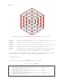
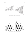
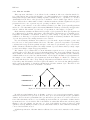
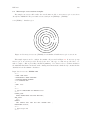
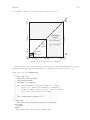
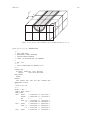
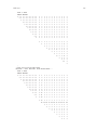
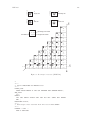
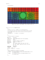
Hexagonal geometry with triangular mesh containing 4 concentric hexagon . . . . .
Diagonal boundary conditions in Cartesian geometry . . . . . . . . . . . . . . . . . .
Various boundary conditions in Cartesian geometry . . . . . . . . . . . . . . . . . . .
Translation/rotation boundary conditions in Cartesian geometry . . . . . . . . . . .
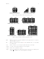
Representing a checkerboard in Cartesian geometry . . . . . . . . . . . . . . . . . . .
Hexagonal geometries of type S30 and SA60 . . . . . . . . . . . . . . . . . . . . . . .
Hexagonal geometries of type SB60 and S90 . . . . . . . . . . . . . . . . . . . . . . .
Hexagonal geometries of type R120 and R180 . . . . . . . . . . . . . . . . . . . . . .
Hexagonal geometry of type SA180 . . . . . . . . . . . . . . . . . . . . . . . . . . . .
Hexagonal geometry of type SB180 . . . . . . . . . . . . . . . . . . . . . . . . . . . .
Hexagonal geometry of type COMPLETE . . . . . . . . . . . . . . . . . . . . . . . .
Cylindrical correction in Cartesian geometry . . . . . . . . . . . . . . . . . . . . . . .
Definition of the radii in a CARCEL– or HEXCEL–type geometry . . . . . . . . . . . . .
Numerotation of the sectors in a Cartesian cell . . . . . . . . . . . . . . . . . . . . .
Numerotation of the sectors in an hexagonal cell . . . . . . . . . . . . . . . . . . . .
Hexagonal geometry with triangular mesh that extends past the hexagonal boundary
Description of the various rotations allowed for Cartesian geometries . . . . . . . . .
Description of the various rotation allowed for hexagonal geometries . . . . . . . . .
Typical cluster geometry . . . . . . . . . . . . . . . . . . . . . . . . . . . . . . . . . .
Organization of a multicompo object. . . . . . . . . . . . . . . . . . . . . . . . . . .
Parameter tree in a multicompo object . . . . . . . . . . . . . . . . . . . . . . . . .
Global parameter tree in a saphyb object . . . . . . . . . . . . . . . . . . . . . . . .
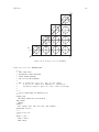
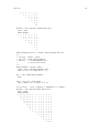
Slab geometry with mesh-splitting . . . . . . . . . . . . . . . . . . . . . . . . . . . .
Two-dimensional Cartesian assembly containing micro-structures . . . . . . . . . . .
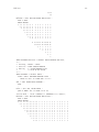
Cylindrical cluster geometry . . . . . . . . . . . . . . . . . . . . . . . . . . . . . . . .
Two-dimensional hexagonal geometry . . . . . . . . . . . . . . . . . . . . . . . . . .
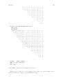
Three-dimensional Cartesian super-cell . . . . . . . . . . . . . . . . . . . . . . . . . .
Hexagonal multicell lattice geometry . . . . . . . . . . . . . . . . . . . . . . . . . . .
Geometry for test case (TCM01) for an annular cell with macroscopic cross sections.
Geometry for test case (TCM02). . . . . . . . . . . . . . . . . . . . . . . . . . . . . .
Geometry for test case (TCM03). . . . . . . . . . . . . . . . . . . . . . . . . . . . . .
Geometry of the CANDU-6 supercell with stainless steel rods. . . . . . . . . . . . . .
Geometry of a 2-D hexagonal assembly filled with triangular/hexagonal cells. . . . .
Geometry for the Mosteller benchmark problem. . . . . . . . . . . . . . . . . . . . .
Geometry for test case (TCWU02). . . . . . . . . . . . . . . . . . . . . . . . . . . . .
Geometry for test case (TCWU03). . . . . . . . . . . . . . . . . . . . . . . . . . . . .
Depletion chain of heavy isotopes. . . . . . . . . . . . . . . . . . . . . . . . . . . . .
Geometry of the CANDU-6 cell. . . . . . . . . . . . . . . . . . . . . . . . . . . . . .
Geometry of 2-D CANDU–6 supercell with control rods. . . . . . . . . . . . . . . . .
An example of depletion chain. . . . . . . . . . . . . . . . . . . . . . . . . . . . . . .
Distribution content. . . . . . . . . . . . . . . . . . . . . . . . . . . . . . . . . . . . .
An example of an associative table. . . . . . . . . . . . . . . . . . . . . . . . . . . . .
.
.
.
.
.
.
.
.
.
.
.
.
.
.
.
.
.
.
.
.
.
.
.
.
.
.
.
.
.
.
.
.
.
.
.
.
.
.
.
.
.
.
.
.
.
.
.
.
.
.
.
.
.
.
.
.
.
.
.
.
.
.
.
.
.
.
.
.
.
.
.
.
.
.
.
.
.
.
.
.
.
.
.
.
.
.
.
.
.
.
.
.
.
.
.
.
.
.
.
.
.
.
.
.
.
.
.
.
.
.
.
.
.
.
.
.
.
.
.
.
.
.
.
.
.
.
32
35
35
36
36
37
37
38
38
39
39
40
44
46
46
47
52
52
52
124
124
141
181
181
182
183
184
185
190
192
194
199
220
223
226
230
233
237
265
279
283
287
IGE–294
ix
List of Tables
1
2
3
4
5
6
7
8
9
10
11
12
13
14
15
16
17
18
19
20
21
22
23
24
25
26
27
28
29
30
31
32
33
34
35
36
37
38
39
40
41
42
43
44
45
46
47
48
49
50
51
52
53
Structure
Structure
Structure
Structure
Structure
Structure
Structure
Structure
Structure
Structure
Structure
Structure
Structure
Structure
Structure
Structure
Structure
Structure
Structure
Structure
Structure
Structure
Structure
Structure
Structure
Structure
Structure
Structure
Structure
Structure
Structure
Structure
Structure
Structure
Structure
Structure
Structure
Structure
Structure
Structure
Structure
Structure
Structure
Structure
Structure
Structure
Structure
Structure
Structure
Structure
Structure
Structure
Structure
(DRAGON) . .
(MAC:) . . . . .
(descmacinp) .
(descxs) . . . . .
(descmacupd) .
(LIB:) . . . . . .
(desclib) . . . .
(desclib) . . . .
(desclib) . . . .
(desclib) . . . .
(descdepl) . . .
(descdeplA2) .
(descmix1) . . .
(descmix2) . . .
(GEO:) . . . . .
(descgtyp) . . .
(descgcnt) . . .
(descBC) . . . .
(descSP) . . . .
(descPP) . . . .
(descDH) . . . .
(descSIJ) . . . .
(desctrack) . . .
(SYBILT:) . . .
(descsybil) . . .
(EXCELT:) . .
(descexcel) . . .
(NXT:) . . . . .
(descnxt) . . . .
(MCCGT:) . . .
(descmccg) . . .
(SNT:) . . . . .
(descsn) . . . . .
(BIVACT:) . . .
(descbivac) . . .
(TRIVAT:) . . .
(descTRIVAC)
(SHI:) . . . . . .
(descshi) . . . .
(USS:) . . . . . .
(descuss) . . . .
(ASM:) . . . . .
(descasm) . . .
(FLU:) . . . . .
(descflu) . . . .
(descleak) . . .
(EDI:) . . . . . .
(descedi) . . . .
(EVO:) . . . . .
(descevo) . . . .
(SPH:) . . . . .
(descsph) . . . .
(CFC:) . . . . .
.
.
.
.
.
.
.
.
.
.
.
.
.
.
.
.
.
.
.
.
.
.
.
.
.
.
.
.
.
.
.
.
.
.
.
.
.
.
.
.
.
.
.
.
.
.
.
.
.
.
.
.
.
.
.
.
.
.
.
.
.
.
.
.
.
.
.
.
.
.
.
.
.
.
.
.
.
.
.
.
.
.
.
.
.
.
.
.
.
.
.
.
.
.
.
.
.
.
.
.
.
.
.
.
.
.
.
.
.
.
.
.
.
.
.
.
.
.
.
.
.
.
.
.
.
.
.
.
.
.
.
.
.
.
.
.
.
.
.
.
.
.
.
.
.
.
.
.
.
.
.
.
.
.
.
.
.
.
.
.
.
.
.
.
.
.
.
.
.
.
.
.
.
.
.
.
.
.
.
.
.
.
.
.
.
.
.
.
.
.
.
.
.
.
.
.
.
.
.
.
.
.
.
.
.
.
.
.
.
.
.
.
.
.
.
.
.
.
.
.
.
.
.
.
.
.
.
.
.
.
.
.
.
.
.
.
.
.
.
.
.
.
.
.
.
.
.
.
.
.
.
.
.
.
.
.
.
.
.
.
.
.
.
.
.
.
.
.
.
.
.
.
.
.
.
.
.
.
.
.
.
.
.
.
.
.
.
.
.
.
.
.
.
.
.
.
.
.
.
.
.
.
.
.
.
.
.
.
.
.
.
.
.
.
.
.
.
.
.
.
.
.
.
.
.
.
.
.
.
.
.
.
.
.
.
.
.
.
.
.
.
.
.
.
.
.
.
.
.
.
.
.
.
.
.
.
.
.
.
.
.
.
.
.
.
.
.
.
.
.
.
.
.
.
.
.
.
.
.
.
.
.
.
.
.
.
.
.
.
.
.
.
.
.
.
.
.
.
.
.
.
.
.
.
.
.
.
.
.
.
.
.
.
.
.
.
.
.
.
.
.
.
.
.
.
.
.
.
.
.
.
.
.
.
.
.
.
.
.
.
.
.
.
.
.
.
.
.
.
.
.
.
.
.
.
.
.
.
.
.
.
.
.
.
.
.
.
.
.
.
.
.
.
.
.
.
.
.
.
.
.
.
.
.
.
.
.
.
.
.
.
.
.
.
.
.
.
.
.
.
.
.
.
.
.
.
.
.
.
.
.
.
.
.
.
.
.
.
.
.
.
.
.
.
.
.
.
.
.
.
.
.
.
.
.
.
.
.
.
.
.
.
.
.
.
.
.
.
.
.
.
.
.
.
.
.
.
.
.
.
.
.
.
.
.
.
.
.
.
.
.
.
.
.
.
.
.
.
.
.
.
.
.
.
.
.
.
.
.
.
.
.
.
.
.
.
.
.
.
.
.
.
.
.
.
.
.
.
.
.
.
.
.
.
.
.
.
.
.
.
.
.
.
.
.
.
.
.
.
.
.
.
.
.
.
.
.
.
.
.
.
.
.
.
.
.
.
.
.
.
.
.
.
.
.
.
.
.
.
.
.
.
.
.
.
.
.
.
.
.
.
.
.
.
.
.
.
.
.
.
.
.
.
.
.
.
.
.
.
.
.
.
.
.
.
.
.
.
.
.
.
.
.
.
.
.
.
.
.
.
.
.
.
.
.
.
.
.
.
.
.
.
.
.
.
.
.
.
.
.
.
.
.
.
.
.
.
.
.
.
.
.
.
.
.
.
.
.
.
.
.
.
.
.
.
.
.
.
.
.
.
.
.
.
.
.
.
.
.
.
.
.
.
.
.
.
.
.
.
.
.
.
.
.
.
.
.
.
.
.
.
.
.
.
.
.
.
.
.
.
.
.
.
.
.
.
.
.
.
.
.
.
.
.
.
.
.
.
.
.
.
.
.
.
.
.
.
.
.
.
.
.
.
.
.
.
.
.
.
.
.
.
.
.
.
.
.
.
.
.
.
.
.
.
.
.
.
.
.
.
.
.
.
.
.
.
.
.
.
.
.
.
.
.
.
.
.
.
.
.
.
.
.
.
.
.
.
.
.
.
.
.
.
.
.
.
.
.
.
.
.
.
.
.
.
.
.
.
.
.
.
.
.
.
.
.
.
.
.
.
.
.
.
.
.
.
.
.
.
.
.
.
.
.
.
.
.
.
.
.
.
.
.
.
.
.
.
.
.
.
.
.
.
.
.
.
.
.
.
.
.
.
.
.
.
.
.
.
.
.
.
.
.
.
.
.
.
.
.
.
.
.
.
.
.
.
.
.
.
.
.
.
.
.
.
.
.
.
.
.
.
.
.
.
.
.
.
.
.
.
.
.
.
.
.
.
.
.
.
.
.
.
.
.
.
.
.
.
.
.
.
.
.
.
.
.
.
.
.
.
.
.
.
.
.
.
.
.
.
.
.
.
.
.
.
.
.
.
.
.
.
.
.
.
.
.
.
.
.
.
.
.
.
.
.
.
.
.
.
.
.
.
.
.
.
.
.
.
.
.
.
.
.
.
.
.
.
.
.
.
.
.
.
.
.
.
.
.
.
.
.
.
.
.
.
.
.
.
.
.
.
.
.
.
.
.
.
.
.
.
.
.
.
.
.
.
.
.
.
.
.
.
.
.
.
.
.
.
.
.
.
.
.
.
.
.
.
.
.
.
.
.
.
.
.
.
.
.
.
.
.
.
.
.
.
.
.
.
.
.
.
.
.
.
.
.
.
.
.
.
.
.
.
.
.
.
.
.
.
.
.
.
.
.
.
.
.
.
.
.
.
.
.
.
.
.
.
.
.
.
.
.
.
.
.
.
.
.
.
.
.
.
.
.
.
.
.
.
.
.
.
.
.
.
.
.
.
.
.
.
.
.
.
.
.
.
.
.
.
.
.
.
.
.
.
.
.
.
.
.
.
.
.
.
.
.
.
.
.
.
.
.
.
.
.
.
.
.
.
.
.
.
.
.
.
.
.
.
.
.
.
.
.
.
.
.
.
.
.
.
.
.
.
.
.
.
.
.
.
.
.
.
.
.
.
.
.
.
.
.
.
.
.
.
.
.
.
.
.
.
.
.
.
.
.
.
.
.
.
.
.
.
.
.
.
.
.
.
.
.
.
.
.
.
.
.
.
.
.
.
.
.
.
.
.
.
.
.
.
.
.
.
.
.
.
.
.
.
.
.
.
.
.
.
.
.
.
.
.
.
.
.
.
.
.
.
.
.
.
.
.
.
.
.
.
.
.
.
.
.
.
.
.
.
.
.
.
.
.
.
.
.
.
.
.
.
.
.
.
.
.
.
.
.
.
.
.
.
.
.
.
.
.
.
.
.
.
.
.
.
.
.
.
.
.
.
.
.
.
.
.
.
.
.
.
.
.
.
.
.
.
.
.
.
.
.
.
.
.
.
.
.
.
.
.
.
.
.
.
.
.
.
.
.
.
.
.
.
.
.
.
.
.
.
.
.
.
.
.
.
.
.
.
.
.
.
.
.
.
.
.
.
.
.
.
.
.
.
.
.
.
.
.
.
.
.
.
.
.
.
.
.
.
.
.
.
.
.
.
.
.
.
.
.
.
.
.
.
.
.
.
.
.
.
.
.
.
.
.
.
.
.
.
.
.
.
.
.
.
.
.
.
.
.
.
.
.
.
.
.
.
.
.
.
.
.
.
.
.
.
.
.
.
.
.
.
.
.
.
.
.
.
.
.
.
.
.
.
.
.
.
.
.
.
.
.
.
.
.
.
.
.
.
.
.
.
.
.
.
.
.
.
.
.
.
.
.
.
.
.
.
.
.
.
.
.
.
.
.
.
.
.
.
.
.
.
.
.
.
.
.
.
.
.
.
.
.
.
.
.
.
.
.
.
.
.
.
.
.
.
.
.
.
.
.
.
.
.
.
.
.
.
.
.
.
.
.
.
.
.
.
.
.
.
.
.
.
.
.
.
.
.
.
.
.
.
.
.
.
.
.
.
.
.
.
.
.
.
.
.
.
.
.
.
.
.
.
.
.
.
.
.
.
.
.
.
.
.
.
.
.
.
.
.
.
.
.
.
.
.
.
.
.
.
.
.
.
.
.
.
.
.
.
.
.
.
.
.
.
.
.
.
.
.
.
.
.
.
.
.
.
.
.
.
.
.
.
.
.
.
.
.
.
.
.
.
.
.
.
.
.
.
.
.
.
.
.
.
.
.
.
.
.
.
.
.
.
.
.
.
.
.
.
.
.
3
9
10
12
15
16
16
17
17
17
22
23
24
27
29
29
30
32
41
47
56
57
59
60
60
63
63
67
67
71
71
74
74
76
76
79
79
82
82
84
85
88
88
91
92
94
97
97
107
107
113
114
118
IGE–294
54
55
56
57
58
59
60
61
62
63
64
65
66
67
68
69
70
71
72
73
74
75
76
77
78
79
80
81
82
83
84
85
86
87
88
89
90
91
92
93
94
95
96
97
98
99
100
101
102
103
104
Structure
Structure
Structure
Structure
Structure
Structure
Structure
Structure
Structure
Structure
Structure
Structure
Structure
Structure
Structure
Structure
Structure
Structure
Structure
Structure
Structure
Structure
Structure
Structure
Structure
Structure
Structure
Structure
Structure
Structure
Structure
Structure
Structure
Structure
Structure
Structure
Structure
Structure
Structure
Structure
Structure
Structure
Structure
Structure
Structure
Structure
Structure
Structure
Structure
Structure
Structure
x
(desccfc) . . . .
(INFO:) . . . . .
(info) . . . . . .
(COMPO:) . . .
(compo data1)
(compo data2)
(compo data3)
(compo data4)
(TLM:) . . . . .
(desctlm) . . . .
(M2T:) . . . . .
(M2T data) . .
(CHAB:) . . . .
(CHAB data) .
(CPO:) . . . . .
(desccpo) . . . .
(SAP:) . . . . .
(saphyb data1)
(saphyb data2)
(saphyb data3)
(MC:) . . . . . .
(MC data) . . .
(T:) . . . . . . .
(DMAC:) . . . .
(DMAC data) .
(DREF:) . . . .
(SENS:) . . . . .
(SENS data) . .
(DUO:) . . . . .
(DUO data) . .
(PSP:) . . . . .
(descpsp) . . . .
(equality) . . . .
(UTL:) . . . . .
(DELETE:) . .
(BACKUP:) . .
(RECOVER:) .
(ADD:) . . . . .
(MPX:) . . . . .
(STAT:) . . . . .
(GREP:) . . . .
(MSTR:) . . . .
(FIND0:) . . . .
(ABORT:) . . .
(END:) . . . . .
(DRVMPI:) . .
(SNDMPI:) . .
assertS . . . . . .
assertV . . . . . .
(descmodule) .
(descobject) . .
.
.
.
.
.
.
.
.
.
.
.
.
.
.
.
.
.
.
.
.
.
.
.
.
.
.
.
.
.
.
.
.
.
.
.
.
.
.
.
.
.
.
.
.
.
.
.
.
.
.
.
.
.
.
.
.
.
.
.
.
.
.
.
.
.
.
.
.
.
.
.
.
.
.
.
.
.
.
.
.
.
.
.
.
.
.
.
.
.
.
.
.
.
.
.
.
.
.
.
.
.
.
.
.
.
.
.
.
.
.
.
.
.
.
.
.
.
.
.
.
.
.
.
.
.
.
.
.
.
.
.
.
.
.
.
.
.
.
.
.
.
.
.
.
.
.
.
.
.
.
.
.
.
.
.
.
.
.
.
.
.
.
.
.
.
.
.
.
.
.
.
.
.
.
.
.
.
.
.
.
.
.
.
.
.
.
.
.
.
.
.
.
.
.
.
.
.
.
.
.
.
.
.
.
.
.
.
.
.
.
.
.
.
.
.
.
.
.
.
.
.
.
.
.
.
.
.
.
.
.
.
.
.
.
.
.
.
.
.
.
.
.
.
.
.
.
.
.
.
.
.
.
.
.
.
.
.
.
.
.
.
.
.
.
.
.
.
.
.
.
.
.
.
.
.
.
.
.
.
.
.
.
.
.
.
.
.
.
.
.
.
.
.
.
.
.
.
.
.
.
.
.
.
.
.
.
.
.
.
.
.
.
.
.
.
.
.
.
.
.
.
.
.
.
.
.
.
.
.
.
.
.
.
.
.
.
.
.
.
.
.
.
.
.
.
.
.
.
.
.
.
.
.
.
.
.
.
.
.
.
.
.
.
.
.
.
.
.
.
.
.
.
.
.
.
.
.
.
.
.
.
.
.
.
.
.
.
.
.
.
.
.
.
.
.
.
.
.
.
.
.
.
.
.
.
.
.
.
.
.
.
.
.
.
.
.
.
.
.
.
.
.
.
.
.
.
.
.
.
.
.
.
.
.
.
.
.
.
.
.
.
.
.
.
.
.
.
.
.
.
.
.
.
.
.
.
.
.
.
.
.
.
.
.
.
.
.
.
.
.
.
.
.
.
.
.
.
.
.
.
.
.
.
.
.
.
.
.
.
.
.
.
.
.
.
.
.
.
.
.
.
.
.
.
.
.
.
.
.
.
.
.
.
.
.
.
.
.
.
.
.
.
.
.
.
.
.
.
.
.
.
.
.
.
.
.
.
.
.
.
.
.
.
.
.
.
.
.
.
.
.
.
.
.
.
.
.
.
.
.
.
.
.
.
.
.
.
.
.
.
.
.
.
.
.
.
.
.
.
.
.
.
.
.
.
.
.
.
.
.
.
.
.
.
.
.
.
.
.
.
.
.
.
.
.
.
.
.
.
.
.
.
.
.
.
.
.
.
.
.
.
.
.
.
.
.
.
.
.
.
.
.
.
.
.
.
.
.
.
.
.
.
.
.
.
.
.
.
.
.
.
.
.
.
.
.
.
.
.
.
.
.
.
.
.
.
.
.
.
.
.
.
.
.
.
.
.
.
.
.
.
.
.
.
.
.
.
.
.
.
.
.
.
.
.
.
.
.
.
.
.
.
.
.
.
.
.
.
.
.
.
.
.
.
.
.
.
.
.
.
.
.
.
.
.
.
.
.
.
.
.
.
.
.
.
.
.
.
.
.
.
.
.
.
.
.
.
.
.
.
.
.
.
.
.
.
.
.
.
.
.
.
.
.
.
.
.
.
.
.
.
.
.
.
.
.
.
.
.
.
.
.
.
.
.
.
.
.
.
.
.
.
.
.
.
.
.
.
.
.
.
.
.
.
.
.
.
.
.
.
.
.
.
.
.
.
.
.
.
.
.
.
.
.
.
.
.
.
.
.
.
.
.
.
.
.
.
.
.
.
.
.
.
.
.
.
.
.
.
.
.
.
.
.
.
.
.
.
.
.
.
.
.
.
.
.
.
.
.
.
.
.
.
.
.
.
.
.
.
.
.
.
.
.
.
.
.
.
.
.
.
.
.
.
.
.
.
.
.
.
.
.
.
.
.
.
.
.
.
.
.
.
.
.
.
.
.
.
.
.
.
.
.
.
.
.
.
.
.
.
.
.
.
.
.
.
.
.
.
.
.
.
.
.
.
.
.
.
.
.
.
.
.
.
.
.
.
.
.
.
.
.
.
.
.
.
.
.
.
.
.
.
.
.
.
.
.
.
.
.
.
.
.
.
.
.
.
.
.
.
.
.
.
.
.
.
.
.
.
.
.
.
.
.
.
.
.
.
.
.
.
.
.
.
.
.
.
.
.
.
.
.
.
.
.
.
.
.
.
.
.
.
.
.
.
.
.
.
.
.
.
.
.
.
.
.
.
.
.
.
.
.
.
.
.
.
.
.
.
.
.
.
.
.
.
.
.
.
.
.
.
.
.
.
.
.
.
.
.
.
.
.
.
.
.
.
.
.
.
.
.
.
.
.
.
.
.
.
.
.
.
.
.
.
.
.
.
.
.
.
.
.
.
.
.
.
.
.
.
.
.
.
.
.
.
.
.
.
.
.
.
.
.
.
.
.
.
.
.
.
.
.
.
.
.
.
.
.
.
.
.
.
.
.
.
.
.
.
.
.
.
.
.
.
.
.
.
.
.
.
.
.
.
.
.
.
.
.
.
.
.
.
.
.
.
.
.
.
.
.
.
.
.
.
.
.
.
.
.
.
.
.
.
.
.
.
.
.
.
.
.
.
.
.
.
.
.
.
.
.
.
.
.
.
.
.
.
.
.
.
.
.
.
.
.
.
.
.
.
.
.
.
.
.
.
.
.
.
.
.
.
.
.
.
.
.
.
.
.
.
.
.
.
.
.
.
.
.
.
.
.
.
.
.
.
.
.
.
.
.
.
.
.
.
.
.
.
.
.
.
.
.
.
.
.
.
.
.
.
.
.
.
.
.
.
.
.
.
.
.
.
.
.
.
.
.
.
.
.
.
.
.
.
.
.
.
.
.
.
.
.
.
.
.
.
.
.
.
.
.
.
.
.
.
.
.
.
.
.
.
.
.
.
.
.
.
.
.
.
.
.
.
.
.
.
.
.
.
.
.
.
.
.
.
.
.
.
.
.
.
.
.
.
.
.
.
.
.
.
.
.
.
.
.
.
.
.
.
.
.
.
.
.
.
.
.
.
.
.
.
.
.
.
.
.
.
.
.
.
.
.
.
.
.
.
.
.
.
.
.
.
.
.
.
.
.
.
.
.
.
.
.
.
.
.
.
.
.
.
.
.
.
.
.
.
.
.
.
.
.
.
.
.
.
.
.
.
.
.
.
.
.
.
.
.
.
.
.
.
.
.
.
.
.
.
.
.
.
.
.
.
.
.
.
.
.
.
.
.
.
.
.
.
.
.
.
.
.
.
.
.
.
.
.
.
.
.
.
.
.
.
.
.
.
.
.
.
.
.
.
.
.
.
.
.
.
.
.
.
.
.
.
.
.
.
.
.
.
.
.
.
.
.
.
.
.
.
.
.
.
.
.
.
.
.
.
.
.
.
.
.
.
.
.
.
.
.
.
.
.
.
.
.
.
.
.
.
.
.
.
.
.
.
.
.
.
.
.
.
.
.
.
.
.
.
.
.
.
.
.
.
.
.
.
.
.
.
.
.
.
.
.
.
.
.
.
.
.
.
.
.
.
.
.
.
.
.
.
.
.
.
.
.
.
.
.
.
.
.
.
.
.
.
.
.
.
.
.
.
.
.
.
.
.
.
.
.
.
.
.
.
.
.
.
.
.
.
.
.
.
.
.
.
.
.
.
.
.
.
.
.
.
.
.
.
.
.
.
.
.
.
.
.
.
.
.
.
.
.
.
.
.
.
.
.
.
.
.
.
.
.
.
.
.
.
.
.
.
.
.
.
.
.
.
.
.
.
.
.
.
.
.
.
.
.
.
.
.
.
.
.
.
.
.
.
.
.
.
.
.
.
.
.
.
.
.
.
.
.
.
.
.
.
.
.
.
.
.
.
.
.
.
.
.
.
119
121
121
125
126
129
130
130
132
132
135
135
137
137
139
139
142
143
145
146
148
148
150
151
151
153
155
155
157
157
160
160
162
163
165
166
167
168
169
170
171
173
175
176
177
178
179
281
281
287
288
IGE–294
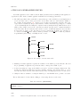
1
1 INTRODUCTION
The computer code DRAGON is a lattice code designed around solution techniques of the neutron
´
Polytechnique de
transport equation.[1] The DRAGON project results from an effort made at Ecole
Montr´eal to rationalize and unify into a single code the different models and algorithms used in a lattice code.[2–5] One of the main concerns was to ensure that the structure of the code was such that the
development and implementation of new calculation techniques would be facilitated. DRAGON is therefore a lattice cell code which is divided into many calculation modules linked together using the GAN
generalized driver[6, 7] . These modules exchange informations only via well defined data structures.
The two main components of the code DRAGON are its multigroup flux solver and its one-group
collision probability (CP) tracking modules. The CP modules all perform the same task but using
different levels of approximation.
The SYBIL tracking option emulates the main flux calculation option available in the APOLLO1 code,[8, 16] and includes a new version of the EURYDICE-2 code which performs reactor assembly
calculations in both rectangular and hexagonal geometries using the interface current method. The
option is activated when the SYBILT: module is called.
The EXCELL tracking option is used to generate the collision probability matrices for the cases
having cluster, two-dimensional or three-dimensional mixed rectangular and cylindrical geometries.[18, 19]
A cyclic tracking option is also available for treating specular boundary conditions in two-dimensional
rectangular geometry.[23, 26] EXCELL calculations are performed using the EXCELT: or NXT: module.
The MCCG tracking option activates the long characteristics solution technique. This implementation
uses the same tracking as EXCELL and perform flux integration using the long characteristics algorithm
proposed by Igor Suslov.[20–22] The option is activated when both EXCELT: (or NXT:) and MCCGT: modules
are called.
After the collision probability or response matrices associated with a given cell have been generated,
the multigroup solution module can be activated. This module uses the power iteration method and
requires a number of iteration types.[30] The thermal iterations are carried out by DRAGON so as to
rebalance the flux distribution only in cases where neutrons undergo up-scattering. The power iterations
are performed by DRAGON to solve the fixed source or eigenvalue problem in the cases where a multiplicative medium is analyzed. The effective multiplication factor (Keff ) is obtained during the power
iterations. A search for the critical buckling may be superimposed upon the power iterations so as to
force the multiplication factor to take on a fixed value.[31]
DRAGON can access directly standard microscopic cross-section libraries in various formats. It has
the capability of exchanging macroscopic cross-section libraries with a code such as TRANSX-CTR or
TRANSX-2 by the use of GOXS format files.[32, 35] The macroscopic cross section can also be read in
DRAGON via the input data stream.
IGE–294
2
2 GENERAL STRUCTURE OF THE DRAGON INPUT
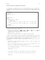
The input to DRAGON is set up in the form of a structure containing commands which call successively each of the calculation modules required in a given transport calculation.
2.1
Data organization
The structure of the input data is independent of the physical or computational characteristics of the
host system. The physical characteristics of the input data is a collection of sequential records. These
characters are by necessity ascii characters. The logical organization of an input deck is in the form of
a sequential structure of input variables presented in free format. This structure must be located in the
first 72 columns of each record in the input stream. Characters located in column 73 and above can be
used to identify the records and are treated as comments. An input variable can be defined in one of two
ways.
• As a set of consecutive characters containing no blanks; it will be considered by DRAGON automatically as being an either an integer, a real or a character variable depending on the format of
the input variable.
• As a set of characters enclosed between quotation marks (’). In this case, the input variable is
always considered to be a character variable.
The only separator allowed between two input variables is a single or a set of blanks (not enclosed
between quotation marks). A single input variable cannot span two records. Comments can be included
in the input deck in one of the following ways:
• characters in column 73 or above on each record are considered to be comments;
• all the information following the ‘;’ keyword on a record are not considered by the generalized
driver;
• each record starting with the characters ‘*’ is considered to be commented out;
• all the characters on a given record inserted between ‘(*’ and ‘’*)’ are considered to be commented
out.
This users guide was written using the following conventions:
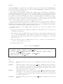
• An input structure represents a set of input variables. It is identified by a name in boldface
surrounded by parenthesis. For example, the complete DRAGON input deck is represented by the
structure (DRAGON);
• A standard DRAGON data structure represents a set records and directory stored in a hierarchical
format on a direct access XSM file or in memory via a linked list.[45] It is identified by a name
in small capital letter. For example, the data structure asmpij contains the multigroup collision
probability matrices generated by the ASM: module of DRAGON;
• The variables presented using the typewriter font are character variables used as keywords. For
example GEO: is the keyword required to activate the geometry reading module of DRAGON.
• The variables in italics are user defined variables. When indexed and surrounded by parenthesis
they denote arrays. If they are in lower case they represent either integer type (starting with
i to n) or real type (starting with a to h or o to z) variables. If they are in upper case they
represent character type variables. For example, iprint must be replaced in the input deck by an
integer variable, (energy(igroup), igroup=1,ngroup+1) states that a vector containing ngroup+1
real elements is to be read while FILE must be replaced by a character variable, its maximum size
being generally specified. No character variable can exceed 72 character in length.
• The variables or structures surrounded by single square brackets ‘[ ]’ are optional.
IGE–294
3
• The variables or structures surrounded by double square brackets ‘[[ ]]’ are also optional. However,
they can be repeated as many times as required.
• The variables or structures surrounded by braces and separated by vertical bars ‘{ | | }’ represents
various calculation options available in DRAGON. Only one of these options is permitted.
When a fixed default value is specified for an optional parameter in a structure, it can be modified
only locally and is reset to the original default value each time the module is called. When a floating
default value is specified for a variable, it is saved and can be used in later calls to this module. In
DRAGON, almost every default value is a floating value, with the exception of the parameter iprint,
which is set to 1 and is used to control the amount of information printed in the module. Departure from
this general rule will be indicated in the following sections.
2.2
DRAGON Data Structure and Module Declarations
DRAGON is built around the GAN generalized driver.[6] Accordingly, all the modules that will be
used during the current execution must be first identified. One must also define the format of each data
structure that will be processed by these modules. Then, the modules required for the specific DRAGON
calculation are called successively, information being transferred from one module to the next via the data
structures. Finally, the execution of DRAGON is terminated when it encounters the END: module even
if it is followed by additional data records in the input data stream. The general input data structure
therefore follows the calling specifications given below:
Table 1: Structure (DRAGON)
[ MODULE [[ MODNAME ]] ; ]
[ LINKED LIST [[ STRNAME ]] ; ]
[ XSM FILE [[ STRNAME ]] ; ]
[ SEQ BINARY [[ STRNAME ]] ; ]
[ SEQ ASCII [[ STRNAME ]] ; ]
[[ (module) ; ]]
END: ;
where
MODULE
keyword used to specify the list of modules to be used in this DRAGON execution.
MODNAME
character*12 name of a DRAGON or utility module. The list of DRAGON module
is provided in Section 2.3 while the list of Utility module is described in Section 2.4.
By default a ‘ ’ module is always available (see Sections 2.4 and 4.1).
LINKED LIST
keyword used to specify which data structures will be stored in linked lists.
XSM FILE
keyword used to specify which data structures will be stored on XSM format files.
SEQ BINARY
keyword used to specify which data structures will be stored on sequential binary files.
SEQ ASCII
keyword used to specify which data structures will be stored on sequential ASCII files.
STRNAME
character*12 name of a DRAGON data structure. Note that on MVS file names are
truncated to 7 characters due to a constraint of this operating system. The list of
DRAGON data structure is presented in Section 2.5.
(module)
input specifications for a DRAGON or utility module. For the DRAGON specific
modules these input structures will be defined in Section 3. For utility modules, the
required structures are described in Section 4.
IGE–294
4
END:
keyword to call the normal end-of-execution utility module.
;
end of record keyword. This keyword is used by DRAGON to delimit the part of the
input data stream associated with each module.
Note that the user generally has the choice to declare most of the data structures in the format of a
linked list to reduce CPU times or as a XSM file to reduce memory resources. Some exceptions to this
general rule are the tracking files as we will see in Section 3.4. In general, the data structure are stored
on the sequential ASCII files only for backup purposes.
The input data normally ends with a call to the END: module (see Section 4.13). However, the GAN
driver will insert automatically the END: module, even if it was not provided, upon reaching an end-of-file
in the input stream.
Each (module) specification contains a description of the execution modules to be called and its
associated input structure. All these modules, except the END: module may be called more than once.
2.3
The DRAGON Modules
The code DRAGON has been divided into main calculations sequences to which is generally associated
a single calculation module. The only exception to this rule is the tracking sequence to which is associated
many different modules, one for each of the standard CP calculation options and an additional module
for diffusion calculations. However, this later module can only be used indirectly in the edition module
of DRAGON. These modules perform the following tasks:
MAC:
module used to generate or modify a DRAGON macrolib (see Section 2.5) which
contains the group ordered macroscopic cross sections for a series of mixture (see
Section 3.1). This macrolib can be either an independent data structure or it can be
included as a substructure in a microlib. The spatial location of these mixtures will
be defined using the GEO: module (see Section 3.3).
LIB:
module used to generate or modify a DRAGON microlib (see Section 2.5) that can
read a number of different types of microscopic cross-section libraries (see Section 3.2).
Each such access requires a double interpolation (temperature, dilution) carried out
by a subroutine specifically tailored to each type of library. Currently the formats
DRAGLIB[45] , WIMS–D4[34] , MATXS[32] , WIMS–AECL[33] , APOLLO[8, 9] and NDAS
format[10] are supported. After having reconstructed the microscopic cross sections for
each isotope, they are then multiplied by the isotopic concentrations (particles per cm3 )
and combined in such a way as to produce an embedded macrolib (see Section 2.5).
The spatial location of these mixtures will be defined using the GEO: module (see
Section 3.3).
GEO:
module used to generate or modify a geometry (see Section 3.3).
SYBILT:
the standard tracking module based on 1D collision probability or Interface Current
technique (see Section 3.4 and Section 3.4.1).
EXCELT:
the standard tracking module for 2D and 3D geometries as well as isolated 2D cells
containing clusters (see Section 3.4 and Section 3.4.2).
NXT:
the standard tracking module for 2D or 3D assemblies of cluster (see Section 3.4 and
Section 3.4.3).
SNT:
the discrete ordinates tracking module (see Section 3.4 and Section 3.4.5).
MCCGT:
the tracking module of the open characteristics flux solver (see Section 3.4 and Section 3.4.4).
BIVACT:
the 1D/2D diffusion and SPn tracking module (see Section 3.4 and Section 3.4.6).
TRIVAT:
the 1D/2D/3D diffusion and SPn tracking module (see Section 3.4 and Section 3.4.7).
IGE–294
5
SHI:
module used to perform self-shielding calculations using the generalized Stamm’ler
method (see Section 3.5).
USS:
module used to perform self-shielding calculations using a subgroup method (see Section 3.6). A method using physical probability tables (cf. Wims-7 and Helios) and the
Ribon extended method are available.
ASM:
module which uses the tracking information to generate a multigroup response or
collision probability matrix (see Section 3.7).
FLU:
module which uses inner-iteration approach or collision probability matrix to solve
the transport equation for the fluxes (see Section 3.8). Various leakage models are
available.
EDI:
editing module (see Section 3.9). An equivalence method based on SPH method is
available.
EVO:
burnup module (see Section 3.10).
SPH:
supermomog´en´eisation (SPH) module (see Section 3.11). The SPH: module can also
be used to extract a microlib or macrolib from a multicompo or saphyb.
INFO:
utility to compute number densities for selected isotopes in materials such as UO2 or
ThUO2 (see Section 3.13).
COMPO:
multi-parameter reactor database construction module (see Section 3.14).
TLM:
module used to generate a Matlab M-file to obtain a graphics representation of the
NXT: tracking lines (see Section 3.15).
M2T:
interface module for transforming a macrolib into a Trimaran/Tripoli multigroup file
(see Section 3.16).
CHAB:
cross section perturbation module similar to CHABINT (see Section 3.17).
CPO:
burnup-dependent mono-parameter reactor database construction module (see Section 3.18).
SAP:
multi-parameter reactor database construction module in SAPHYB format (see Section 3.19).
MC:
multigroup Monte-Carlo flux solution module (see Section 3.20).
T:
macrolib transposition operator (see Section 3.21).
DMAC:
construction module for a Generalized Perturbation Theory (GPT) source (see Section 3.22).
SENS:
sensitivity analysis of keff to nuclear data (see Section 3.24).
PSP:
module to generate PostScript images for 2D geometries that can be tracked using the
module EXCELT: or NXT: (see Section 3.26).
DUO:
module to perform a perturbative analysis of two systems using the Clio formula and
to determine the origins of Keff discrepancies (see Section 3.25).
IGE–294
2.4
6
The Utility Modules
Because the execution of DRAGON is controlled by the GAN generalized driver it can use directly
any one of its utility modules. These modules perform the following tasks:
’ ’
default module used to make an explicit copy of a data structure (see Section 4.1).
UTL:
module used to manipulate a data structure (see Section 4.2).
DELETE:
module used to delete a data structure (see Section 4.3).
BACKUP:
module used to make a backup copy of a child data structure along with its parent
(see Section 4.4).
RECOVER:
module used to recover form a backup copy a child data structure along with its parent
(see Section 4.5).
ADD:
module used to add two data structures (see Section 4.6).
MPX:
module used to multiply a data structure by a constant (see Section 4.7).
STAT:
module used to compare two data structures (see Section 4.8).
GREP:
module used to locate information on a data structure (see Section 4.9).
FIND0:
module used to find the zero of a tabulated function (see Section 4.11).
END:
module used to terminate an execution controlled by the generalized driver (see Section 4.13).
2.5
The DRAGON Data Structures
The transfer of information between the DRAGON execution modules is ensured by well defined data
structure. They are generally created or modified directly by one of the modules of DRAGON or by one
of the utility modules. Here we will give a brief description of these data structures but a more complete
description of their content is also available upon request.[45] These data structures are memory-resident
or persistent (i.e., XSM–type) objects.
macrolib
a standard data structure used by DRAGON to transfer group-ordered macroscopic
cross sections between its modules. It can be a stand-alone structure or it can be
included into a larger structure, such as a microlib or an edition structure. It can
be created by the MAC:, LIB: and EDI: modules. It can also be modified by the SHI:,
USS: and EVO: modules. Such a structure (either stand-alone or as part of a microlib)
is also required for a successful execution of the ASM: and FLU: modules.
microlib
a standard data structure used by DRAGON to transfer microscopic and macroscopic
cross sections between its modules. It always include a macrolib substructure. It
can be a stand-alone structure or included into a larger structure, such as an edition
structure. It can be created by the LIB: and EDI: modules. It can also be modified
by the MAC:, SHI:, USS: and EVO: modules.
geometry
a standard data structure used by DRAGON to transfer the geometry between its
modules. It can be a stand-alone structure or included into a larger structure, such as
another geometry structure. It can be created by the GEO: module. Such a structure
is also required directly for a successful execution of the tracking modules (SYBILT:,
EXCELT: and MCCGT:).
tracking
a standard data structure used by DRAGON to transfer the general tracking information between its modules. It is a stand-alone structure. It can be created by the
SYBILT:, EXCELT: and MCCGT: modules. Such a structure is also required directly for
a successful execution of the ASM: module.
IGE–294
7
asmpij
a standard data structure used by DRAGON to transfer the multigroup response and
collision probability matrices between its modules. It is a stand-alone structure. It is
created by the ASM: module. Such a structure is also required directly for a successful
execution of the FLU: module.
fluxunk
a standard data structure used by DRAGON to transfer the fluxes between its modules.
It is a stand-alone structure. It is created by the FLU: module. Such a structure is
also required for a successful execution of the EDI: and EVO: modules.
edition
a standard data structure used by DRAGON to store condensed and merged microscopic and macroscopic cross sections. It is a stand-alone structure but can contain
macrolib and microlib substructure. It is created by the EDI: module. Such a
structure is also required for a successful execution of the COMPO: module.
burnup
a standard data structure used by DRAGON to store burnup informations. It is created
by the EVO: module. Such a structure is also required for a successful execution of the
COMPO: module.
draglib
a standard data structure used by DRAGON (input) to recover isotopic–, dilution– and
temperature–dependent information, including multigroup microscopic cross sections
and burnup data. This is a stand-alone structure that is generally stored on a persistent
LCM object. It may be created by the dragr module of NJOY.
cpo
a standard data structure used by DRAGON to store a simplified reactor dabase. It
is a stand-alone structure that must be stored on a linked list or an XSM file. It
is created by the CPO: module. It is required for a successful execution of the CFC:
module. It can be used by the CRE: module of DONJON.
multicompo
a standard data structure used by DRAGON (output) to store reactor related information and to classified it using tuples of local and global parameters. This is a
stand-alone structure that is generally stored on a persistent LCM object. It is created
by the COMPO: module.
saphyb
a standard data structure used by APOLLO2 and DRAGON (output) to store reactor
related information and to classified it using tuples of global parameters. This is a
stand-alone structure that is generally stored on a persistent LCM object. It is created
by the SAP: module.
fbmxsdb
a standard data structure used by DRAGON to store a full reactor cross section
database with Feedback coefficients. It is a stand-alone structure that must be stored
on a linked list or an XSM file. It is created by the CFC: module. It can be used by
the AFM: module of DONJON.[86]
2.6
Main Updates in DRAGON
The frozen version (DRAGON Release 3.06) has seen a large number of changes since the first official
release of the code (DRAGON 960627).
The current DRAGON package (DRAGON Version4) is an evolution of the frozen version, released
as an attempt to introduce innovative capabilities:
• The new self-shielding module USS: allow increased accuracy and better representation of phenomena such as distributed self-shielding effects and mutual self-shielding effects.
• The new flux solution solver MCCG is an implementation of the long characteristics method proposed by Igor Suslov. This solver is initiated by the new tracking module MCCGT:.
• The new flux solution module FLU: is a complete rewrite of the outer iteration for the multigroup
flux calculation that is now compatible with the method of characteristics and with any other
approach requiring inner iterations. The MOCC: module is no longer required.
IGE–294
8
• The burnup module EVO: was extended to take into account energy produced by radioactive decay
and by reactions other than fission.
• The new module COMPO: is used to create and increment a multiparameter reactor database. The
module The companion module NCR: is used to interpolate an existing multiparameter reactor
database.
• The flux solution solver SYBIL related to 2D assembly calculations was extended to allow sectorization of the cells.
• The method of discrete ordinates is implemented in tracking module SNT:.
• The EXCELL: module has been removed, but its capability is now implemented using the XCLL
keyword in EXCELT:.
• The LIB: module can access NDAS-formatted cross-section libraries.
IGE–294
9
3 THE DRAGON MODULES
The input to DRAGON is set up in the form of a structure containing commands which call successively each of the calculation modules required in a given transport calculation.
3.1
The MAC: module
In DRAGON, the macroscopic cross sections associated with each mixture are stored in a macrolib
(as an independent data structure or as part of a microlib) which may be generated using one of different
ways:
• First, one can use directly the input stream already used for the remaining DRAGON data. In this
case, a single macroscopic library is involved.
• The second method is via a GOXS format binary sequential file.[32] It should be noted that a number
of GOXS files may be read successively by DRAGON and that it is possible to combine data from
GOXS files with data taken from the input stream. One can also transfer the macroscopic cross
sections to a GOXS format binary file if required. In this case, a single macroscopic library is
involved.
• The third input method is through a file which already contains a macrolib. In this case, two
macroscopic and microscopic libraries are to be combined
• The fourth method consists to update an existing macrolib using control-variable data recovered
from a L OPTIMIZE object.
The general format of the data for the MAC: module is the following:
Table 2: Structure (MAC:)
{ MACLIB := MAC: [ MACLIB ] :: (descmacinp)
| MICLIB := MAC: MICLIB :: (descmacinp)
| MACLIB := MAC: [ MACLIB ] [ OLDLIB ] :: (descmacupd)
| MACLIB := MAC: MACLIB OPTIM ;
}
The meaning of each of the terms above is:
MACLIB
character*12 name of a macrolib that will contain the macroscopic cross sections.
If MACLIB appears on both LHS and RHS, it is updated; otherwise, it is created. If
MACLIB is created, all macroscopic cross sections are first initialized to zero.
MICLIB
character*12 name of a microlib. Only the macrolib data substructure of this
microlib is then updated. This is used mainly to associate fixed sources densities
with various mixtures. If any other cross section is modified for a specific mixture, the
microscopic and macroscopic cross sections are no longer compatible. One can return
to a compatible library using the library update module (see Section 3.2).
OLDLIB
character*12 name of a macrolib or a microlib which will be used to update or
create the MACLIB macrolib.
OPTIM
character*12 name of a L OPTIMIZE object. The macrolib MACLIB is updated
using control-variable data recovered from OPTIM .
(descmacinp)
macroscopic input data structure for this module (see Section 3.1.1).
IGE–294
(descmacupd)
10
macroscopic update data structure for this module (see Section 3.1.3).
3.1.1 Input structure for module MAC:
In the case where there are no OLDLIB specified, the (descmac) input structure takes the form:
Table 3: Structure (descmacinp)
[ EDIT iprint ]
[ NGRO ngroup ]
[ NMIX nmixt ]
[ NIFI nifiss ]
[ DELP ndel ]
[ ANIS naniso ]
[ CTRA { NONE | APOL | WIMS | LEAK } ]
[ NALP nalbp ]
[ ALBP (albedp(ia),ia=1,nalbp) ]
[ WRIT GOXSWN ]
[ ENER (energy(jg), jg=1,ngroup +1) ]
[ VOLUME (volume(ibm), ibm=1,nmixt) ]
[ ADD ]
[[ { READ [ (imat(i), i=1,nmixt) ] GOXSRN [ DELE ] | READ INPUT [[ (descxs) ]] } ]]
[[ STEP istep READ INPUT [[ (descxs) ]] ]]
[ NORM ]
;
with
EDIT
keyword used to modify the print level iprint.
iprint
index used to control the printing in this module. It must be set to 0 if no printing on
the output file is required. The macroscopic cross sections can written to the output
file if the variable iprint is greater than or equal to 2. The transfer cross sections will
be printed if this parameter is greater than or equal to 3. The normalization of the
transfer cross sections will be checked if iprint is greater than or equal to 5.
NGRO
keyword to specify the number of energy groups for which the macroscopic cross sections will be provided. This information is required only if MACLIB is created and
the cross sections are taken directly from the input data stream.
ngroup
the number of energy groups used for the calculations in DRAGON. The default value
is ngroup=1.
NMIX
keyword used to define the number of material mixtures. This information is required
only if MACLIB is created and the cross sections are taken directly from the input
data stream or from a GOXS file.
nmixt
the maximum number of mixtures (a mixture is characterized by a distinct set of
macroscopic cross sections) the macrolib may contain. The default value is nmixt=1.
NIFI
keyword used to specify the maximum number of fissile spectrum associated with each
mixture. Each fission spectrum generally represents a fissile isotope. This information
IGE–294
11
is required only if MACLIB is created and the cross sections are taken directly from
the input data stream.
nifiss
the maximum number of fissile isotopes per mixture. The default value is nifiss=1.
DELP
keyword used to specify the number of delayed neutron groups.
ndel
the number of delayed neutron groups. The default value is ndel=0.
ANIS
keyword used to specify the maximum level of anisotropy permitted in the scattering
cross sections. This information is required only if MACLIB is created and the cross
sections are taken directly from the input data stream.
naniso
number of Legendre orders for the representation of the scattering cross sections. The
default value is naniso=1 corresponding to the use of isotropic scattering cross sections.
CTRA
keyword to specify the type of transport correction that should be generated and stored
on the macrolib. The transport correction is to be substracted from the total and
isotropic (P0 ) within-group scattering cross sections. A leakage correction, equal to
the difference between current– and flux–weighted total cross sections (Σ1 − Σ0 ) is also
applied in the APOL and LEAK cases. All the modules that will read this macrolib
will then have access to transport corrected cross sections. The default is no transport
correction when the macrolib is created from the input or GOXS files.
NONE
keyword to specify that no transport correction should be used in this calculation.
APOL
keyword to specify that an APOLLO type transport correction based on the linearly
anisotropic (P1 ) scattering cross sections is to be set. This correction assumes that the
micro-reversibility principle is valid for all energy groups. P1 scattering information
must exists in the macrolib.
WIMS
keyword to specify that a WIMS–type transport correction is used. The transport
correction is recovered from a record named TRANC. This record must exists in the
macrolib.
LEAK
A leakage correction is applied to the total and P0 within-group scattering cross sections. No transport correction is applied in this case.
NALP
keyword to specify the maximum number of physical albedos which will be read. These
can be used by the GEO: module (see Section 3.3).
nalbp
the maximum number of physical albedos. The default value is nalbp=1.
ALBP
keyword used for the input of the physical albedo array.
albedp
physical albedo array. A maximum of nalbp entries can be specified.
WRIT
keyword used to write cross section data to a GOXS file. In the case where nifiss>1,
this option is invalid.
GOXSWN
character*7 name of the GOXS file to be created or updated.
ENER
keyword to specify the energy group limits.
energy
energy (eV) array which define the limits of the groups (ngroup+1 elements). Generally energy(1) is the highest energy.
VOLUME
keyword to specify the mixture volumes.
volume
volume (cm3 ) occupied by each mixture.
ADD
keyword for adding increments to existing macroscopic cross sections. In this case, the
information provided in (descxs) represents incremental rather than standard cross
sections.
IGE–294
12
READ
keyword to specify the input file format. One can use either the input stream (keyword
INPUT) or a GOXS format file.
imat
array of mixture identifiers to be read from a GOXS file. The maximum number of
identifiers permitted is nmixt and the maximum value that imat may take is nmixt.
When imat is 0, the corresponding mixture on the GOXS file is not included in the
macrolib. In the cases where imat is absent all the mixtures on the GOXS file are
available in a DRAGON execution. They are numbered consecutively starting at 1 or
from the last number reached during a previous execution of the MAC: module.
GOXSRN
character*7 name of the GOXS file to be read.
DELE
keyword to specify that the GOXS file is deleted after being read (Revision 3.03
only).
INPUT
keyword to specify that mixture cross sections will be read on the input stream.
(descxs)
structure describing the format used for reading the mixture cross sections from the
input stream (see Section 3.1.2).
STEP
keyword used to create a perturbation directory.
istep
the index of the perturbation directory.
NORM
keyword to specify that the macroscopic scattering cross sections and the fission spectrum have to be normalized. This option is available even if the mixture cross sections
were not read by the MAC: module.
3.1.2 Macroscopic cross section definition
Table 4: Structure (descxs)
MIX [ matnum ]
[ { NTOT0 | TOTAL } (xssigt(jg), jg=1,ngroup) ]
[ NTOT1 (xssig1(jg), jg=1,ngroup) ]
[ TRANC (xsstra(jg), jg=1,ngroup) ]
[ NUSIGF ((xssigf (jf,jg), jg=1,ngroup), jf=1,nifiss) ]
[ CHI ((xschi(jf,jg), jg=1,ngroup), jf=1,nifiss)]
[ FIXE (xsfixe(jg), jg=1,ngroup) ]
[ DIFF (diff (jg), jg=1,ngroup) ]
[ DIFFX (xdiffx(jg), jg=1,ngroup) ]
[ DIFFY (xdiffy(jg), jg=1,ngroup) ]
[ DIFFZ (xdiffz(jg), jg=1,ngroup) ]
[ NUSIGD (((xssigd(jf,idel,jg), jg=1,ngroup), idel=1,ndel), jf=1,nifiss) ]
[ CHDL (((xschid(jf,idel,jg), jg=1,ngroup), idel=1,ndel), jf=1,nifiss)]
[ OVERV (overv(jg), jg=1,ngroup) ]
[ NFTOT (nftot(jg), jg=1,ngroup) ]
[ FLUX-INTG (xsint0(jg), jg=1,ngroup) ]
[ FLUX-INTG-P1 (xsint1(jg), jg=1,ngroup) ]
[ H-FACTOR (hfact(jg), jg=1,ngroup) ]
[ SCAT (( nbscat(jl,jg), ilastg(jl,jg),(xsscat(jl,jg,ig),
ig=1,nbscat(jl,jg) ), jg=1,ngroup), jl=1,naniso) ]
IGE–294
13
MIX
keyword to specify that the macroscopic cross sections associated with a new mixture
are to be read.
matnum
identifier for the next mixture to be read. The maximum value permitted for this
identifier is nmixt. When matnum is absent, the mixtures are numbered consecutively
starting with 1 or with the last mixture number read either on the GOXS or the input
stream.
NTOT0
keyword to specify that the total macroscopic cross sections for this mixture follows.
TOTAL
alias keyword for NTOT0.
xssigt
array representing the multigroup total macroscopic cross section (Σg in cm−1 ) associated with this mixture.
NTOT1
keyword to specify that the P1 –weighted total macroscopic cross sections for this mixture follows.
xssig1
array representing the multigroup P1 –weighted total macroscopic cross section (Σg1 in
cm−1 ) associated with this mixture.
TRANC
keyword to specify that the transport correction macroscopic cross sections for this
mixture follows.
xsstra
array representing the multigroup transport correction macroscopic cross section (Σgtc
in cm−1 ) associated with this mixture.
NUSIGF
keyword to specify that the macroscopic fission cross section multiplied by the average
number of neutrons per fission for this mixture follows.
xssigf
array representing the multigroup macroscopic fission cross section multiplied by the
average number of neutrons per fission (νΣgf in cm−1 ) for all the fissile isotopes associated with this mixture.
CHI
keyword to specify that the fission spectrum for this mixture follows.
xschi
array representing the multigroup fission spectrum (χg ) for all the fissile isotopes associated with this mixture.
FIXE
keyword to specify that the fixed neutron source density for this mixture follows.
xsfixe
array representing the multigroup fixed neutron source density for this mixture (S g in
s−1 cm−3 ).
DIFF
keyword to specify that the isotropic diffusion coefficient for this mixture follows.
diff
array representing the multigroup isotropic diffusion coefficient for this mixture (Dg
in cm).
DIFFX
keyword for input of the X–directed diffusion coefficient.
xdiffx
array representing the multigroup X–directed diffusion coefficient (Dxg in cm) for the
mixture matnum.
DIFFY
keyword for input of the Y –directed diffusion coefficient.
xdiffy
array representing the multigroup Y –directed diffusion coefficient (Dyg in cm) for the
mixture matnum.
DIFFZ
keyword for input of the Z–directed diffusion coefficient.
xdiffz
array representing the multigroup Z–directed diffusion coefficient (Dzg in cm) for the
mixture matnum.
IGE–294
14
NUSIGD
keyword to specify that the delayed macroscopic fission cross section multiplied by the
average number of neutrons per fission for this mixture follows.
xssigd
array representing the delayed multigroup macroscopic fission cross section multiplied
by the average number of neutrons per fission (νΣg,idel
in cm−1 ) for all the fissile
f
isotopes associated with this mixture.
CHDL
keyword to specify that the delayed fission spectrum for this mixture follows.
xschid
array representing the delayed multigroup fission spectrum (χg,idel ) for all the fissile
isotopes associated with this mixture.
OVERV
keyword for input of the multigroup average of the inverse neutron velocity.
overv
array representing the multigroup average of the inverse neutron velocity (< 1/v >gm )
for the mixture matnum.
NFTOT
keyword for input of the multigroup macroscopic fission cross sections.
nftot
array representing the multigroup macroscopic fission cross section (Σgf ) for the mixture matnum.
FLUX-INTG
keyword for input of the multigroup P0 volume-integrated fluxes.
xsint0
array representing the multigroup P0 volume-integrated fluxes (V φg0 ) for the mixture
matnum.
FLUX-INTG-P1
keyword for input of the multigroup P1 volume-integrated fluxes.
xsint1
array representing the multigroup P1 volume-integrated fluxes (V φg1 ) for the mixture
matnum.
H-FACTOR
keyword to specify that the power factor for this mixture follows.
hfact
array representing the multigroup power factor for this mixture (H g in M eV cm−1 ).
SCAT
keyword to specify that the macroscopic scattering cross section matrix for this mixture
follows.
nbscat
array representing the number of primary groups ig with non vanishing macroscopic
scattering cross section towards the secondary group jg considered for each anisotropy
level associated with this mixture.
ilastg
array representing the group index of the most thermal group with non-vanishing
macroscopic scattering cross section towards the secondary group jg considered for
each anisotropy level associated with this mixture.
xsscat
ig→jg
array representing the multigroup macroscopic scattering cross section (Σsl
in
cm−1 ) from the primary group ig towards the secondary group jg considered for each
anisotropy level associated with this mixture. The elements are ordered using decreasing primary group number ig, from ilastg to (ilastg−nbscat+1), and an increasing
secondary group number jg. Examples of input structures for macroscopic scattering
cross sections can be found in Section 6.1.
3.1.3 Update structure for operator MAC:
In the case where OLDLIB is specified, the (descmacupd) input structure takes the form:
IGE–294
15
Table 5: Structure (descmacupd)
[ EDIT iprint ]
[ CTRA OFF ]
[[ MIX numnew [ numold { UPDL | OLDL } ] ]]
;
with
EDIT
keyword used to modify the print level iprint.
iprint
index used to control the printing in this operator. It must be set to 0 if no printing on
the output file is required. The macroscopic cross sections can written to the output file if
the variable iprint is greater than or equal to 2. The transfer cross sections will be printed
if this parameter is greater than or equal to 3. The normalization of the transfer cross
sections will be checked if iprint is greater than or equal to 5.
CTRA
keyword to specify the type of transport correction that should be generated and stored
on the macrolib. All the operators that will read this macrolib will then have access to
transport corrected cross sections. In the case where the macrolib is updated using other
macrolib or microlib the default is to use a transport correction whenever one of these
older data structure requires a transport correction.
OFF
deactivates the transport correction.
MIX
keyword to specify that the macroscopic cross sections associated with a mixture is to be
created or updated.
numnew
mixture number to be updated or created on the output macrolib.
numold
mixture number on an old macrolib or microlib which will be used to update or create
numnew on the output macrolib
OLDL
the macroscopic cross sections associated with mixture numold are taken from OLDLIB.
This is the default option.
UPDL
the macroscopic cross sections associated with mixture numold are taken from MACLIB.
IGE–294
3.2
16
The LIB: module
The general format of the input data for the LIB: module is the following:
Table 6: Structure (LIB:)
MICLIB := LIB: [ MICLIB [ OLDLIB ] ] :: (desclib)
where
MICLIB
character*12 name of the microlib that will contain the internal library. If MICLIB
appears on both LHS and RHS, it is updated; otherwise, it is created.
OLDLIB
character*12 name of a read-only macrolib, microlib or burnup data structure.
In the case where a macrolib is considered, it is included directly in the MICLIB
before updating it. If it is a second microlib or a burnup data structure, the number
densities for the isotopes in file MICLIB will be replaced selectively by those found in
OLDLIB.
(desclib)
input structure for this module (see Section 3.2.1).
3.2.1 Data input for module LIB:
In the case where OLDLIB is absent or represents a macrolib, (desclib) takes the form:
Table 7: Structure (desclib)
[
[
[
[
[
[
[
[
[
[
[
EDIT iprint ]
NGRO ngroup ]
MXIS nmisot ]
NMIX nmixt ]
CALENDF ipreci ]
CTRA { NONE | APOL | WIMS | OLDW | LEAK } ] [ ANIS naniso ]
ADJ ]
PROM ]
{ SKIP | INTR | SUBG | PT | PTMC | PTSL | NEWL } ] [ MACR ]
ADED nedit ( HEDIT(i), i=1,nedit ) ]
DEPL { LIB: { DRAGON | WIMS | WIMSD4 | WIMSAECL | NDAS } FIL: NAMEFIL
| LIB: { APLIB2 | APXSM } FIL: NAMEFIL (descdeplA2)
| ndepl (descdepl) } ]
[[ MIXS LIB:
{ DRAGON | MATXS | MATXS2 | WIMS | WIMSD4 | WIMSAECL | NDAS | APLIB1 | APLIB2 | APXSM }
FIL: NAMEFIL [[ (descmix1) ]] ]]
It is possible to reset an existing microlib (i.e., MICLIB is present in the RHS) and to reprocess all the
isotopes from the cross section libraries. In this case, (desclib) takes the simplified form:
IGE–294
17
Table 8: Structure (desclib)
[ EDIT iprint ]
{ INTR | SUBG | PT | PTMC | PTSL | NEWL } [ MACR ]
MIXS ;
Alternatively if OLDLIB is absent or represents a second microlib, (desclib) takes the form:
Table 9: Structure (desclib)
[ EDIT iprint ]
MAXS [[ (descmix2) ]]
Finally, if OLDLIB represents burnup structure, (desclib) takes the form:
Table 10: Structure (desclib)
[ EDIT iprint ]
BURN { iburn | tburn } [[ (descmix2) ]]
with
EDIT
keyword used to modify the print level iprint.
iprint
index used to control the printing in this operator. It must be set to 0 if no printing on
the output file is required while values >0 will increase in steps the amount of information
transferred to the output file. If iprint≥10, the depletion chain is printed in the format
of structure (descdepl). If iprint≥20, the depletion chain is also printed in the format of
structure (descdeplA2).
MXIS
keyword used to redefine the maximum number of isotopes per mixture.
nmisot
the maximum number of isotopes per mixture. By default up to 300 different isotopes per
mixture are permitted.
NMIX
keyword used to define the number of material mixtures. This data is required if MICLIB
is created.
nmixt
the maximum number of mixtures (a mixture is characterized by a distinct set of macroscopic cross sections).
CALENDF
keyword to set the accuracy of the CALENDF probability tables.
ipreci
integer set to 1, 2, 3 or 4. The highest the value, the more accurate are the probability
tables.
CTRA
keyword to specify the type of transport correction that should be generated and stored on
the microlib. The transport correction is to be substracted from the total and isotropic
IGE–294
18
(P0 ) within-group scattering cross sections. A leakage correction, equal to the difference
between current– and flux–weighted total cross sections (σ1 − σ0 ) is also applied in the
APOL, OLDW and LEAK cases. All the operators that will read this microlib will then have
access to transport corrected cross sections. The default is no transport correction.
NONE
keyword to specify that no transport correction should be used in this calculation.
APOL
keyword to specify that an APOLLO type transport correction based on the linearly
anisotropic (P1 ) within-group scattering cross sections is to be set. This correction assumes that the micro-reversibility principle is valid for all energy groups. This type of
correction uses P1 scattering information present on the library.
WIMS
This type of correction uses directly a transport-correction provided on the library. Such
information is available in WIMSD4 and WIMS–AECL libraries. This is the new recommended option with WIMS-type libraries. This option has no effect on libraries that does
not contain transport correction information.
OLDW
keyword to specify that a WIMS type transport correction based on the P1 scattering cross
sections is to be set. This correction assumes that the micro-reversibility principle is valid
only for groups energies less than 4.0 eV. For the remaining groups a 1/E current spectrum
is considered in the evaluation of the transport correction. This type of correction uses P1
scattering information present on the library.
LEAK
A leakage correction is applied to the total and P0 within-group scattering cross sections.
No transport correction is applied in this case.
ANIS
keyword to specify the maximum level of anisotropy for the scattering cross sections.
naniso
number of Legendre orders for the representation of the scattering cross sections. Isotropic
scattering is represented by naniso=1 while naniso=2 represents linearly anisotropic scattering. Generally the linearly anisotropic (P1 ) scattering contributions are taken into account via the transport correction (see CTRA keyword) in the transport calculation. For B1
or P1 leakage calculations, the linearly anisotropic scattering cross sections are taken into
account explicitly. The default value is naniso=2.
ADJ
keyword to specify the production of adjoint macroscopic cross sections. By default, direct
cross sections are produced.
PROM
keyword to specify that prompt neutrons are to be considered for the calculation of the
fission spectrum. By default, the contribution due to delayed neutrons is considered. This
option is only compatible with a MATXS or MATXS2 format library.
SKIP
keyword to recover the user–defined microlib data without processing any library (i.e.,
without temperature and/or dilution interpolation).
INTR
keyword to perform a temperature and dilution interpolation of the microscopic cross
sections present in the libraries. The bin-type cross-section data is not processed. This is
the default option.
SUBG
keyword to activate the calculation of the physical probability tables using the temperature-interpolated cross-section data as input.[11, 13] The bin-type cross-section data is not
processed.
PT
keyword to activate the calculation of the CALENDF-type mathematical probability tables
(without slowing-down correlated weight matrices) using the bin-type cross-section data
as input.[12] This option is compatible with the Sanchez-Coste self-shielding method and
with the subgroup projection method (SPM).[14]
PTMC
this option is similar to the PT procedure. Here, the base points of the probability tables
corresponding to fission and scattering cross sections and to components of the transfer
scattering matrix are also obtained using the CALENDF approach.
IGE–294
19
PTSL
keyword to activate the calculation of the CALENDF-type mathematical probability tables and slowing-down correlated weight matrices using the bin-type cross-section data as
input.[13]
NEWL
keyword to activate the calculation of a DRAGLIB library using the temperature-interpolated cross-section data as input. The bin-type cross-section data is processed.
MACR
keyword to force the calculation of the embedded macrolib. By default, the embedded
macrolib is computed, except if one of the key words SKIP, INTR, SUBG, PT or NEWL is used.
ADED
keyword to specify the input of additional cross sections to be treated by DRAGON. These
cross sections are not needed to solve the transport equation but are recognized by the
EDI: and utility operators.
nedit
number of types of additional cross sections.
HEDIT
character*6 name of an additional cross-section type. This name also corresponds to
vectorial reactions in a MATXS and MATXS2 format library. For example:
NWT0/NWT1=P0/P1 library weight functions.
NTOT0/NTOT1=P0/P1 neutron total cross sections.
NELAS=Neutron elastic scattering cross sections (MT=2).
NINEL=Neutron inelastic scattering cross sections (MT=4).
NG=Neutron radiative capture cross sections (MT=102).
NFTOT=Total fission cross sections (MT=18).
NUDEL=Number of delayed secondary neutrons (Nu-D / MT=455).
NFSLO=ν∗slow fission cross section.
NHEAT=Heat production cross section.
CHIS/CHID=Slow/delayed fission spectrum.
NF/NNF/N2NF/N3NF=ν∗partial fission cross sections (MT=19, 20, 21 and 38).
N2N/N3N/N4N=(n,2n), (n,3n), (n,4n) cross sections (MT=16, 17 and 37).
NP/NA=(n,p) and (n,α) transmutation cross sections (MT=103 and 107).
By default, DRAGON will always attempt to recover the additional cross sections NG,
NFTOT, NHEAT and N2N which are required for the depletion calculations.
DEPL
keyword to specify that the isotopic depletion (burnup) chain is to be read. For a given
LIB: execution only one isotopic depletion chain can be read.
MIXS
keyword to specify that the mixture description is to be read. For a given LIB: execution
more than one cross-section library can be read.
LIB:
keyword to specify the type of library from which the isotopic depletion chain or microscopic
cross section is to be read. It is optional when preceded by the keyword DEPL in which case
the isotopic depletion chain is read from the standard input file.
DRAGON
keyword to specify that the isotopic depletion chain or the microscopic cross sections are
in the DRAGLIB format.
MATXS
keyword to specify that the microscopic cross sections are in the MATXS format of NJOY-II
and NJOY-89 (no depletion data available for libraries using this format).
MATXS2
keyword to specify that the microscopic cross sections are in the MATXS format of NJOY91 (no depletion data available for libraries using this format).
WIMSD4
keyword to specify that the isotopic depletion chain and the microscopic cross sections are
in the WIMSD4 format.
WIMS
keyword to specify that the isotopic depletion chain and the microscopic cross sections are
in the WIMS-AECL format.
IGE–294
20
WIMSAECL
keyword to specify that the isotopic depletion chain and the microscopic cross sections are
in the WIMS-AECL format.
NDAS
keyword to specify that the isotopic depletion chain and the microscopic cross sections are
in the NDAS format, as used in recent versions of WIMS-AECL.
APLIB1
keyword to specify that the microscopic cross sections are in the APOLLO-1 format. There
are no depletion chains available for libraries using this format.
APLIB2
keyword to specify that the microscopic cross sections are in the APOLLO-2 direct access
format. There are no depletion chains available for libraries using this format. However,
fission yields, radioactive decay constants and energy released per fission or radiative capture are recovered from the file. Only versions of the APOLIB-2 libraries subsequent or
equal to CEA93-V4 can be processed. The list of isotopes (standard and self-shielded)
available in an APOLIB-2 is printed by setting the print flag to a value iprint≥10.
APXSM
keyword to specify that the microscopic cross sections are in the APOLIB-XSM format,
the output format of N2A2 utility. There are no depletion chains available for libraries
using this format. However, fission yields, radioactive decay constants and energy released
per fission or radiative capture are recovered from the file. The list of isotopes (standard
and self-shielded) available in an APOLIB-XSM is printed by setting the print flag to a
value iprint≥10.
FIL:
keyword to specify the name of the file where is stored the isotopic depletion data.
NAMEFIL
character*64 name of the library where the isotopic depletion chain or the microscopic
cross sections are stored. Library names in DRAGLIB format are limited to 12 characters.
A NDAS library is made of two or more files. These file names must be concatenated in a
single NAMEFIL name, using semicolumns as separators. The ascii index file is always
the first, followed by optional patch files, and terminated by the main direct-access binary
file. The following sample data line corresponds to a ndas library without patch:
MIXS LIB: NDAS FIL: E65LIB6.idx:E65LIB6.sdb
ndepl
number of isotopes in the depleting chain.
(descdepl)
input structure describing the depletion chain (see Section 3.2.2).
(descdeplA2) simplified input structure describing the depletion chain in cases where an APOLIB-2 or
APOLIB-XSM file is used (see Section 3.2.2).
MAXS
keyword to specify that the mixture density on MICLIB are to be modified. If OLDLIB is
present and (descmix2) is absent, a direct one to one correspondence between the isotope
on both libraries is assumed. If OLDLIB and (descmix2) are present, only the mixture on
the library file specified by (descmix2) are updated using information from the OLDLIB.
If OLDLIB is absent and (descmix2) is present, only the mixture on MICLIB specified
by (descmix2) are updated.
BURN
keyword to specify that the mixture density on MICLIB are to be updated using information taken from OLDLIB. If (descmix2) is absent, a direct one to one correspondence
between the isotope on OLDLIB and MICLIB is assumed. If (descmix2) is present, only
the mixture specified by (descmix2) are updated using information from OLDLIB.
iburn
burnup step from the burnup file to use. This step must be already present on the burnup
file.
tburn
burnup time in days from the burnup file to use. This time step must be already present
on the burnup file.
IGE–294
21
(descmix1) input structure describing the isotopic and physical properties of a given mixture (see
Section 3.2.3).
(descmix2) input structure describing perturbations to the isotopic and physical properties of a given
mixture (see Section 3.2.3).
Note that it is possible to recompute the embedded macrolib in an existing microlib named MICRO by
writing
MICRO := LIB: MICRO :: MACR MIXS ;
IGE–294
22
3.2.2 Depletion data structure
The structure (descdepl) describes the heredity of the radioactive decay and the neutron activation
chain to be used in the isotopic depletion calculation.
Table 11: Structure (descdepl)
CHAIN
[[ NAMDPL [ izae ]
[[ { DECAY dcr |
reaction [ energy ] } ]]
[ { STABLE |
FROM [[ { DECAY | reaction } [[ yield NAMPAR ]] ]] } ] ]]
ENDCHAIN
with:
CHAIN
keyword to specify the beginning of the depletion chain.
NAMDPL
character*12 name of an isotope (or isomer) of the depletion chain that appears in the
cross-section library.
izae
optional six digit integer representing the isotope. The first two digits represent the atomic
number of the isotope; the next three indicate its mass number and the last digit indicates
the excitation level of the nucleus (0 for a nucleus in its ground state, 1 for an isomer in
its first exited state, etc.). For example, 238 U in its ground state will be represented by
izae=922380.
DECAY
indicates that a decay reaction takes place either for production of this isotope or its
depletion.
dcr
radioactive decay constant (in 10−8 s−1 ) of the isotope. By default, dcr=0.0.
reaction
character*6 identification of a neutron-induced reaction that takes place either for production of this isotope, its depletion, or for producing energy. Example of reactions are
following:
NG
indicates that a radiative capture reaction takes place either for production of this isotope, its depletion or for producing energy.
N2N
indicates that the following reaction is taking place:
n +A XZ → 2n +A−1 XZ
N3N
indicates that the following reaction is taking place:
n +A XZ → 3n +A−2 XZ
N4N
indicates that the following reaction is taking place:
n +A XZ → 4n +A−3 XZ
NP
indicates that the following reaction is taking place:
n +A XZ → p +A YZ−1
IGE–294
23
NA
indicates that the following reaction is taking place:
n +A XZ →4 He2 +A−3 XZ−2
NFTOT
indicates that a fission is taking place.
energy
energy (in MeV) recoverable per neutron-induced reaction of type reaction. If the energy
associated to radiative capture is not explicitely given, it should be added to the energy
released per fission. By default, energy=0.0 MeV.
STABLE
non depleting isotope. Such an isotope may produces energy by neutron-induced reactions
(such as radiative capture).
FROM
indicates that this isotope is produced from decay or neutron-induced reactions.
yield
branching ratio or production yield expressed in fraction.
NAMPAR
character*12 name of the a parent isotope (or isomer) that appears in the cross-section
library.
ENDCHAIN
keyword to specify the end of the depletion chain.
If the keyword APLIB2 or APXSM was used in structure (desclib), part of the depletion data is recovered
from the APOLIB file: the fission yields, the radioactive decay constants and the energy released per
fission or radiative capture. Moreover, the following simplified structure is used to provide the remaining
depletion data:
Table 12: Structure (descdeplA2)
CHAIN
[[ NAMDPL [ FROM [[ { DECAY | reaction } yield NAMPAR ]] ] ]]
ENDCHAIN
In this case, the following rules apply:
• We should provide the names NAMDPL of all the depleting isotopes (i.e. isotopes with a timedependent number density), including the pseudo fission products (PFP).
• The fission father reactions (NFTOT) are not given.
• The stable isotopes are automatically recovered from the APOLIB file. They are not given in
structure (descdeplA2).
• An isotope is considered to be stable if it is not present in structure (descdeplA2), has no father
and no daughter, but can release energy by fission or radiative capture.
• It is possible to truncate the isotope name NAMDPL at the underscore. For example, D2O 3 P5
can be simply written D2O.
• Only the radioactive decay constants of the isotopes present in structure (descdeplA2) are recovered from the APOLIB file. The radioactive decay constants of the other isotopes are set to
zero.
IGE–294
24
3.2.3 Mixture description structure
The structure (descmix1) is used to describe the isotopic composition and the physical properties,
such as the temperature and density, of a mixture.
Table 13: Structure (descmix1)
MIX [ matnum ] {
[temp [ denmix ] ] [ NOEV ]
[[ [ NAMALI = ] NAMISO dens [ { dil | INF } ]
[ [ CORR ] inrs ] [ DBYE tempd ] [ SHIB NAMS ] [ THER ntfg HINC [ TCOH HCOH ] ]
[ IRSET { gir | { PT | PTMC | PTSL} } { nir | NONE } ] [ { NOEV | SAT } ] ]]
|
COMB [[ mati relvol ]] }
where:
MIX
keyword to specify the number identifying the next mixture to be read.
matnum
mixture identifier. The maximum value that matnum may have is nmixt. When matnum
is absent, the mixtures are numbered successively starting from 1 if no mixture has yet
been specified or from the last mixture number specified + 1.
temp
absolute temperature (in Kelvin) of the isotopic mixture. It is optional only when this
mixture is to be updated, in which case the old temperature associated with the mixture
is used.
denmix
mixture density in g cm−3 .
NAMALI
character*8 alias name for an isotope to be used locally. When the alias name is absent,
the isotope name used locally is identical to the first 8-character isotope name on the
library.
=
keyword to specify to which isotope in a library is associated the previous alias name.
NAMISO
character*12 name of an isotope present in the library which is included in this mixture.
dens
isotopic concentration of the isotope NAMISO in the current mixture in 1024 cm−3 . When
the mixture density denmix is specified, the relative weight percentage of each of the
isotopes in this mixture is to be provided.
dil
group independent microscopic dilution cross section (in barns) of the isotope NAMISO
in this mixture. It is possible to recalculate a group dependent dilution for an isotope by
the use of the SHI: operator (see Section 3.5). In this case, the dilution is only used as a
starting point for the self-shielding iterations and has no effect on the final result. If the
dilution is not given or is larger than 1010 barns, an infinite dilution is assumed.
INF
keyword to specify that a dilution of 1010 barns is to be associated with this isotope. This
value represents an infinite dilution (the isotope is present in trace amounts only). It is
possible to recalculate a group dependent dilution for an isotope by the use of the SHI:
operator (see Section 3.5). In this case, the dilution is only used as a starting point for the
self-shielding iterations and has no effect on the final result. If the dilution is not given an
infinite dilution is assumed.
IGE–294
25
CORR
keyword to specify that the resonances of an isotope are correlated with those of other
isotopes with the same inrs index. This option is only available with the Ribon extended
model[13] or wth the subgroup projection method (SPM)[14] in energy groups where this
model is set. If this option is selected for an isotope, it must be set for all isotopes with
the same inrs index. By default, the resonances of distinct isotopes are assumed to be
uncorrelated.
inrs
index of the resonant region associated with this isotope. By default inrs=0 and the isotope
is not a candidate for self-shielding. When inrs6=0, the isotope can be self-shielded where
it is assumed that a given isotope distributed with different concentrations in a number of
mixtures and having the same value of inrs will share the same fine flux. Should we wish
to self-shield both the clad and the fuel it is important to assign a different inrs number
to each. If a single type of fuel is located in different mixture in onion-peel fashion, it is
necessary to attribute a single inrs value to this fuel.
DBYE
keyword to specify that the absolute temperature of the isotope is different from that of
the isotopic mixture. This option is useful to define Debye-corrected temperature.
tempd
absolute temperature (in Kelvin) of the isotope. By default tempd=temp.
SHIB
keyword to specify that the name of the isotope containing the information related to the
self-shielding is different from the initial name of the isotope. This option is not required
if a MATXS or a DRAGLIB file is used.
NAMS
character*12 name of a record in the library containing the self-shielding data. This
name is required if the dilution is not infinite or a non zero resonant region is associated
with this isotope and NAMS is different from NAMISO. This record must be contained in
the same library file as record NAMISO.
THER
keyword to specify that the thermalization effects are to be included with the cross sections
when using a MATXS or MATXS2 format library.
HINC
character*6 name of the incoherent thermalization effects which will be taken into account. The incoherent effects are those that may be described by the S(α, β) scattering
law. The value FREE is used to simulate the effects of a gas.
TCOH
keyword to specify that coherent thermalization effects will be taken into account.
HCOH
character*6 name of the coherent thermalization effects which will be taken into account.
The coherent effects are the vectorial reactions in the MATXS or MATXS2 format library
where the name is terminated by the ‘$’ suffix. They are generally available for graphite,
beryllium, beryllium oxide, polyethylene and zirconium hydroxide.
ntfg
number of energy groups that will be affected by the thermalization effects.
IRSET
keyword to specify an intermediate resonance (IR) approximation or the Ribon extended
model for some energy groups. By default, an IR approximation with the value of the
Goldstein-Cohen parameter found on the library is used. If no value is found on the
library, a statistical (ST) model[15] is set in all groups by default.
gir
imposed Goldstein-Cohen IR parameter. A Goldstein-Cohen IR parameter 0 ≤ λg ≤ 1 is
set in energy group g. A value of 1.0 stands for a statistical (ST) approximation. A value
of 0.0 stands for an infinite mass (IM or WR) approximation.
PT
keyword to enable the calculation of CALENDF–type probability tables in some energy
groups. The slowing-down correlated weight matrices are not computed. This type of
probability tables is consistent with the Sanchez-Coste self-shielding method and with the
subgroup projection method (SPM).[14]
IGE–294
26
PTMC
keyword to enable the calculation of CALENDF–type probability tables, similar to the
PT procedure. Here, the base points of the probability tables corresponding to fission
and scattering cross sections and to components of the transfer scattering matrix are also
obtained using the CALENDF approach.
PTSL
keyword to enable the calculation of CALENDF–type probability tables, consistent with
the Ribon extended model, in some energy groups.
nir
the intermediate resonance (IR) approximation or the Ribon extended model is imposed
for energy groups with an index equal or greater than nir. A statistical (ST) model is set
in other groups.
NONE
keyword to specify that a statistical (ST) model is set in all groups.
NOEV
keyword to force a mixture or a nuclide to be non-depleting (even in cases where it is
potentially depleting). Note that the mixture or nuclide keeps its capability to produce
energy. By default, the depleting isotopes are automatically regognized as depleting.
SAT
keyword to force a nuclide to be at saturation. By default, the saturation approximation
is automatically set as a function of the half life and capture cross sections of the isotope.
COMB
keyword to specify that this mixture is reset with a combination of previously defined
mixtures.
mati
number associated with a previously defined mixture. In order to insert some void in a
mixture use mati=0. If the mixture is not already defined one assumes that it represents
a voided mixture.
relvol
relative volume Vi occupied by mixture mati=i in matnum. Two cases can be considered,
namely that where the density ρi of each mixture mati is provided along with the weight
percent for each isotope J (Wij ) and the case where the explicit concentration Nij of each
isotope in a mati was provided (it is forbidden to combined two mixtures with different
isotopic content description). In the case where the initial mixtures are defined using
densities ρi , the density (ρk ) and volume (Vk ) of the final mixture will become:
X
Vi
Vk =
i
ρk =
1 X
ρi Vi
Vk i
and the weight percent will be changed in a consistent way, namely
Wk,J =
ρi Vi Wi,J
ρk Vk
When the explicit concentration are given we will use:
Nk,J =
Vi Ni,J
Vk
There is a very common usage of keyword COMB. In the following example, a new mixture
with index 42 is defined in such a way to be identical to an existing mixture with index 25.
MIX 42 COMB 25 1.0
Note that in the structure (descmix1) one only needs to describe the isotopes initially present in each
mixture. DRAGON will then automatically associate with each depleting mixture the additional isotopes
required by the available burnup chain. Moreover, the microscopic cross-section library associated with
these new isotopes will be the same as that of their parent isotope. For example, suppose that mixture 1
IGE–294
27
contains isotope U235 which is to be read on the DRAGON-formatted library associated with file DRAGLIB.
Assume also that the depletion chain, which is written on the WIMS–AECL format library associated
with file WIMSLIB, states that isotope U236 (initially absent in the mixture) can be generated form U235
by neutron capture. Then, one can either specify explicitly from which library file the microscopic cross
sections associated with isotope U236 (zero concentration) are to be read, or omit U236 from the mixture
description in which case DRAGON will assume that the microscopic cross sections associated with
isotope U236 are to be read from the same library as the cross section for isotope U235. Note that the
isotopes added automatically will remain at infinite dilution.
If the SHI: module implementing the generalized Stamm’ler method is used, the self-shielding data
for an isotope takes the form
U235
= U235
5.105E-5 1
where the last index indicates the self-shielding region (1 in this case).
If the USS: module implementing the subgroup method is used, additional self-shielding data is required:
• Physical probability tables are used (keyword SUBG). Consider the following data:
U235
= U235
5.105E-5 1 IRSET 0.0 81
The data “IRSET 0.0 81” indicates that a Goldstein-Cohen parameter λg equal to 0.0 is used for
all energy groups with an index equal or greater than 81. A value of λg = 1.0 corresponding to a
statistical model is used by default.
• Mathematical probability tables (with slowing-down correlated weight matrices) are used (keyword
PTSL) or mathematical probability tables with the subgroup projection method (SPM)[14] are used
(keyword PT or PTMC). Consider the following data:
U235
= U235
5.105E-5 1 IRSET PT 5
The Goldstein-Cohen approximation is not used with mathematical (CALENDF) probability tables.
The data “IRSET PT 5” indicates that the CALENDF probability tables are used for energy groups
with an index equal or greater than 5, with the exception of the energy groups where no Autolib
data is available and a statistical model (with physical probability tables) is used for energy groups
with an index smaller than 5. A statistical model is also imposed in groups where no Autolib data
is available.
The following data:
U235
= U235
5.105E-5 1 IRSET PT NONE
is useful to impose the statistical model (with physical probability tables) in all energy groups.
The structure (descmix2) is used to describe the modifications in the isotopic composition of a
mixture.
Table 14: Structure (descmix2)
MIX matnum [ matold ] [ relden ] [ NAMALI dens ] [ NOEV ]
where:
IGE–294
28
MIX
keyword to specify the number identifying the next mixture to be updated.
matnum
mixture identifier on MICLIB.
matold
mixture identifier on OLDLIB.
relden
relative density of updated mixture. The concentration of each isotope in the mixture is to
be multiplied by this factor whether it comes from MICLIB, from OLDLIB or is specified
explicitly using dens.
NAMALI
character*8 alias name for an isotope on MICLIB to be modified.
dens
isotopic concentration of the isotope NAMISO in the current mixture in 1024 cm−3 . When
relden is specified, the isotopic concentration becomes dens×relden.
NOEV
keyword to force a mixture to be non-depleting (even in cases where it is potentially
depleting). Note that the mixture keeps its capability to produce energy.
IGE–294
3.3
29
The GEO: module
The GEO: module is used to create or modify a geometry. The geometry definition module in DRAGON
permits all the characteristics (coordinates, region mixture and boundary conditions) of a simple or
complex geometry to be specified. The method used to specify the geometry is independent of the
discretization module to be used subsequently. Each geometry is stored in the form of a geometry data
structure under its given name. It is always possible to modify an existing geometry or copy it under a
new name. The calling specifications are:
Table 15: Structure (GEO:)
{
GEONAM := GEO: { GEONAM | OLDGEO } :: (descgcnt)
|
GEONAM := GEO: :: (descgtyp) (descgcnt)
}
where
GEONAM
character*12 name of the geometry created or modified.
OLDGEO
character*12 name of a read-only geometry. The type and all the characteristics
of OLDGEO will be copied onto GEONAM before this later geometry is modified.
(descgtyp)
structure describing the geometry type of GEONAM (see Section 3.3.1).
(descgcnt)
structure describing the characteristics of a geometry (see Section 3.3.1).
3.3.1 Data input for module GEO:
Structures (descgtyp) and (descgcnt) are used to define respectively the type of geometry that
will be define and the contents of this geometry (dimensions, materials, boundary conditions). The
module GEO: can be recursively called from (descgcnt) as an embedded module, in order to define
sub-geometries:
Table 16: Structure (descgtyp)
{ VIRTUAL |
HOMOGE |
SPHERE lr |
CAR1D lx |
CAR2D lx ly |
CAR3D lx ly lz |
TUBE lr [ lx ly ] |
TUBEX lr { lx | lx ly lz } |
TUBEY lr { ly | lx ly lz } |
TUBEZ lr { lz | lx ly lz } |
RTHETA lr lz |
continued on next page
IGE–294
30
Structure (descgtyp)
continued from last page
HEX lh |
HEXZ lh lz |
HEXT nhr |
HEXTZ nhr lz |
CARCEL lr [ lx ly ] |
CARCELX lr { lx | lx ly lz } |
CARCELY lr { ly | lx ly lz } |
CARCELZ lr { lz | lx ly lz } |
HEXCEL lr |
HEXCELZ lr lz |
GROUP lp }
Table 17: Structure (descgcnt)
[ EDIT iprint ]
(descBC)
(descSP)
(descPP)
(descDH)
(descSIJ)
[[ ::: SUBGEO := GEO: { (descgtyp) | SUBGEO | OLDGEO } (descgcnt)]]
;
where
VIRTUAL
keyword to specify that a virtual geometry description follows. This type of geometry
is used to complete an assembly that has irregular boundaries.
HOMOGE
keyword to specify that a infinite homogeneous geometry description follows.
SPHERE
keyword to specify that a spherical geometry (concentric spheres) description follows.
CAR1D
keyword to specify that a one dimensional plane geometry (infinite slab) description
follows.
CAR2D
keyword to specify that a two-dimensional Cartesian geometry description follows.
CAR3D
keyword to specify that a three-dimensional Cartesian geometry description follows.
TUBE
keyword to specify that a cylindrical geometry (infinite tubes or cylinders) description
follows. This geometry can contain an imbedded X − Y Cartesian mesh.
TUBEX
keyword to specify that a polar R − X cylindrical geometry description follows. This
geometry can contain an imbedded Y − Z Cartesian mesh.
TUBEY
keyword to specify that a polar R − Y cylindrical geometry description follows. This
geometry can contain an imbedded Z − X Cartesian mesh.
TUBEZ
keyword to specify that a polar R − Z cylindrical geometry description follows. This
geometry can contain an imbedded X − Y Cartesian mesh.
IGE–294
31
RTHETA
keyword to specify that a polar geometry (R − θ) description follows.
HEX
keyword to specify that a two-dimensional hexagonal geometry description follows.
HEXZ
keyword to specify that a three-dimensional hexagonal geometry description follows.
HEXT
keyword to specify a single 2-D hexagonal cell geometry having a triangular mesh.
This option is only supported by the NXT: tracking module (see Section 3.4).
HEXTZ
keyword to specify a single Z directed 3-D hexagonal cell geometry having a triangular
mesh (plane X − Y ). This option is only supported by the NXT: tracking module (see
Section 3.4).
CARCEL
keyword to specify that a two-dimensional mixed Cartesian cell (concentric tubes surrounded by a rectangle) description follows. The rectangle can now be subdivided into
a fine mesh when the EXCELT: modules is used.
CARCELX
keyword to specify that a three-dimensional mixed Cartesian cell with tubes oriented
along the X−axis description follows. The three-dimensional Cartesian cell can now
be subdivided into a fine mesh when the EXCELT: module is used.
CARCELY
keyword to specify that a three-dimensional mixed Cartesian cell with tubes oriented
along the Y −axis description follows. The three-dimensional Cartesian cell can now
be subdivided into a fine mesh when the EXCELT: module is used.
CARCELZ
keyword to specify that a three-dimensional mixed Cartesian cell with tubes oriented
along the Z−axis description follows. The three-dimensional Cartesian cell can now
be subdivided into a fine mesh when the EXCELT: module is used.
HEXCEL
keyword to specify that a two-dimensional mixed hexagonal cell (concentric tubes
surrounded by a hexagon) description follows.
HEXCELZ
keyword to specify that a three-dimensional mixed hexagonal cell with tubes oriented
along the Z−axis description follows.
GROUP
keyword to specify that a do-it-yourself type geometry description follows.
lx
number of subdivisions along the X−axis (before mesh-splitting).
ly
number of subdivisions along the Y −axis (before mesh-splitting).
lz
number of subdivisions along the Z−axis (before mesh-splitting).
lr
number of cylinders or spherical shells (before mesh-splitting).
lh
number of hexagons in an axial plane (including the virtual hexagon).
nhr
number of concentric hexagons in a HEXT or HEXTZ cell (see Figure 1). This will lead
to an hexagon subdivided into 6N 2 identical trangles.
lp
number of types of cells (number of cells inside which a distinct flux will be calculated)
for a do-it-yourself type geometry.
EDIT
keyword used to modify the print level iprint.
iprint
index used to control the printing in this module. It must be set to 0 if no printing
on the output file is required, to 1 for minimum printing (fixed default value) and to
2 for printing the geometry state vector.
(descBC)
structure allowing the boundary conditions surrounding the geometry to be treated
(see Section 3.3.2).
(descSP)
structure allowing the coordinates of a geometry to be described (see Section 3.3.3).
IGE–294
32
-9
-10
-11
-12
46
58 55
-15
-16
36
62
53 51
59 56
50
63
54 52
60 57
67
64
71 69
72
77 74
-17
42
78 75
-18
79
-19
-7
27 31
-6
-5
27 20
39 25
47 43
48 44
40
-13 61
41 38
-14
-8
45 32
37
26 29
22 24
21 23
16 -4
35 20
34
18 19
9 12
4 6
15 -3
33 17
1 2
49
8 11
3 5
14 -2
65 81
66
82 84
7 10
13 -1
68 83
86 89
70
85 88
92 96
-24
73 82
91 95
-23
72
90 94
-22
80 93
-20
-21
Figure 1: Hexagonal geometry with triangular mesh containing 4 concentric hexagon
(descPP)
structure allowing material mixtures to be associated with a geometry (see Section 3.3.4).
(descDH)
structure used to specify double-heterogeneity data (see Section 3.3.5).
(descSIJ)
structure used to specify the properties of do-it-yourself geometries (see Section 3.3.6).
SUBGEO
character*12 name of the directory that will contain the sub-geometry.
OLDGEO
character*12 name of a parallel directory containing an existing sub-geometry. The
type and all the characteristics of OLDGEO will be copied onto SUBGEO.
Note that all the geometry described above are called pure geometry when they do not contain subgeometry. When they do contain sub-geometry they will be called composite geometry.
3.3.2 Boundary conditions
The inputs corresponding to the (descBC) structure are the following:
Table 18: Structure (descBC)
[ X- { VOID | REFL | SSYM | DIAG | TRAN |
| CYLI | ACYL { albedo | icode } }
[ X+ { VOID | REFL | SSYM | DIAG | TRAN |
| CYLI | ACYL { albedo | icode } }
[ Y- { VOID | REFL | SSYM | DIAG | TRAN |
| CYLI | ACYL { albedo | icode } }
SYME | ALBE { albedo | icode } | ZERO | PI/2 | PI
]
SYME | ALBE { albedo | icode } | ZERO | PI
]
SYME | ALBE { albedo | icode } | ZERO | PI/2 | PI
]
continued on next page
IGE–294
33
Structure (descBC)
continued from last page
[ Y+ { VOID | REFL | SSYM | DIAG | TRAN | SYME | ALBE { albedo | icode } | ZERO | PI
| CYLI | ACYL { albedo | icode } } ]
[ Z- { VOID | REFL | SSYM | TRAN | SYME | ALBE { albedo | icode } | ZERO } ]
[ Z+ { VOID | REFL | SSYM | TRAN | SYME | ALBE { albedo | icode } | ZERO } ]
[ R+ { VOID | REFL | ALBE { albedo | icode } | ZERO } ]
[ HBC { S30 | SA60 | SB60 | S90 | R120 | R180 | SA180 | SB180 | COMPLETE }
{ VOID | REFL | SYME | ALBE { albedo | icode } | ZERO } ]
[ RADS [ ANG ] nrads (xrad(ir), rrad(ir) [, ang(ir) ], ir=1,nrads ) ]
where:
X-/X+
keyword to specify the boundary conditions associated with the negative or positive X surface
of a Cartesian geometry.
Y-/Y+
keyword to specify the boundary conditions associated with the negative or positive Y surface
of a Cartesian geometry.
Z-/Z+
keyword to specify the boundary conditions associated with the negative or positive Z surface
of a Cartesian geometry.
R+
keyword to specify the boundary conditions associated with the outer surface of a cylindrical
or spherical geometry.
HBC
keyword to specify the boundary conditions associated with the outer surface of an hexagonal
geometry.
VOID
keyword to specify that the surface under consideration has zero re-entrant angular flux. This
side is an external surface of the domain.
REFL
keyword to specify that the surface under consideration has a reflective boundary condition.
In most DRAGON calculations, this implies white boundary conditions. The main exception to this rule is when cyclic tracking in 2-D is considered and mirror like reflections are
considered. A geometry is never unfolded to take into account a REFL boundary condition.
SSYM
keyword to specify that the surface under consideration has a specular (or mirror) reflective
boundary condition. The main difference between REFL and SSYM is that for SSYM the cell
may be unfolded to take into account the reflection at the boundary.
DIAG
keyword to specify that the Cartesian surface under consideration has the same properties as
that associated with a diagonal through the geometry (see Figure 2). Note that two and only
two DIAG surfaces must be specified. The diagonal symmetry is only permitted for square
geometry and in the following combinations:
X+ DIAG Y- DIAG
or
X- DIAG Y+ DIAG
TRAN
keyword to specify that the surface under consideration is connected to the opposite surface
of a Cartesian domain (see Figure 3). This option provides the facility to treat an infinite geometry with translation symmetry. The only combinations of translational symmetry
permitted are:
• Translation along the X−axis
IGE–294
34
X- TRAN X+ TRAN
• Translation along the Y −axis
Y- TRAN Y+ TRAN
• Translation along the Z−axis
Z- TRAN Z+ TRAN
SYME
keyword to specify that the Cartesian surface under consideration is virtual and that a
reflection symmetry is associated with the adequately directed axis running through the
center of the cells closest to this surface (see Figure 3). Only the hexagonal geometries S30
and SA60 can be surrounded by a SYME boundary condition if a specular condition is to be
applied on this boundary.
ALBE
keyword to specify that the surface under consideration has an arbitrary albedo. This side
is an external surface of the domain.
albedo
geometric albedo corresponding to the boundary condition ALBE (albedo>0.0).
icode
index of a physical albedo corresponding to the boundary condition ALBE. The numerical
values of the physical albedo are supplied by the operator MAC: (see Section 3.1).
ZERO
keyword to specify that the surface under consideration has a zero-flux boundary condition.
This side is an external surface of the domain.
PI/2
keyword to specify that the surface under consideration has a π/2 rotational symmetry (see
Figure 3). The only π/2 symmetry permitted is related to sides (X- and Y-). This condition
can be combined with a translation boundary condition:(PI/2 X- TRAN X+) and/or (PI/2
Y- TRAN Y+) (see Figure 4).
PI
keyword to specify that the surface under consideration has a π rotational symmetry (see
Figure 3). This keyword is useful for representing a Cartesian checkerboard pattern as shown
in Fig. 5.
CYLI
the side under consideration has a zero incoming current boundary condition with a circular
correction applied on the Cartesian boundary. This option is only available in the X–Y plane
for CAR2D and CAR3D geometries defined for TRIVAC full–core calculations.
ACYL
the side under consideration has an arbitrary albedo with a circular correction applied on
the Cartesian boundary. This option is only available in the X–Y plane for CAR2D and CAR3D
geometries defined for TRIVAC full–core calculations.
S30
keyword to specify an hexagonal symmetry of one twelfth of an assembly (see Figure 6).
SA60
keyword to specify an hexagonal symmetry of one sixth of an assembly of type A (see Figure 6).
SB60
keyword to specify an hexagonal symmetry of one sixth of an assembly of type B (see Figure 7).
S90
keyword to specify an hexagonal symmetry of one quarter of an assembly (see Figure 7).
R120
keyword to specify a rotation symmetry of one third of an assembly (see Figure 8).
R180
keyword to specify a rotation symmetry of a half assembly (see Figure 8).
SA180
keyword to specify an hexagonal symmetry of half a type A assembly (see Figure 9).
SB180
keyword to specify an hexagonal symmetry of half a type B assembly (see Figure 10).
COMPLETE
keyword to specify a complete hexagonal assembly (see Figure 11).
IGE–294
35
a
di
side 3
Assembly without symmetries
side 2
si
side 3
de
al
n
go
side 2
side 2
side 2
side 1
side 4
side 3
side 3
DIAG condition on sides 1 and 4
Figure 2: Diagonal boundary conditions in Cartesian geometry
side 4
side 4
side 4
side 4
side 2
side 1
side 1
side 1
side 4
side 3
side 3
side 3
Condition TRAN on sides 1 and 2
side 3
side 3
Condition ALBE or REFL on side 2
side 4
Condition SYME on side 3
side 4
side 2
side 4
side 3
side 4
side 2
side 2
side 2
side 1
side 4
side 4
side 2
side 2
side 3
side 4
Condition PI on side 1
side 4
side 2
Condition PI/2 on sides 1 and 3
Figure 3: Various boundary conditions in Cartesian geometry
RADS
This key word is used to specify the cylindrical correction applied in the X − Y plane for
CAR2D and CAR3D geometries.[17]
ANG
This key word allows the angle (see Figure 12) of the cylindrical notch to be set. By default,
no notch is present.
nrads
Number of different corrections along the cylinder main axis (i.e. the Z axis).
xrad(ir)
Coordinate of the Z axis from which the correction is applied.
rrad(ir)
Radius of the real cylindrical boundary.
ang(ir)
Angle of the cylindrical notch. This data is given if and only if the key word ANG is present.
ang(ir) = π2 by default (i.e. the correction is applied at every angle).
IGE–294
36
side 4
side 2
side 4
side 4
side 2
side 4
side 2
side 4
side 2
side 2
side 4
side 4
side 2
side 2
side 4
side 2
Condition PI/2 on sides 1 and 3 and condition TRAN on sides 2 and 4
Figure 4: Translation/rotation boundary conditions in Cartesian geometry
side 4
side 4
side 4
side 4
side 2
side 1
side 2
side 1
side 4
side 1
side 2
side 2
side 1
side 1
side 2
side 3
Condition PI on side 3 and TRAN on sides 1, 2 and 4
Figure 5: Representing a checkerboard in Cartesian geometry
IGE–294
37
S30
9
6
4
8
2
5
1
3
7
12
CL
SA60
11
10
21
15
10
CL
CL
6
3
9
1
5
8
2
4
7
20
14
19
13
18
12
17
11
16
CL
Figure 6: Hexagonal geometries of type S30 and SA60
CL
27
CL
25
19
18
13
SB60
12
5
16
7
2
10
6
3
CL
1
22
15
21
9
5
2
14
23
16
11
10
9
24
17
7
15
6
3
12
11
4
1
18
17
8
S90
26
14
8
4
Figure 7: Hexagonal geometries of type SB60 and S90
20
13
CL
IGE–294
38
31
21
29
4
2
3
31
28
19
13
12
20
27
18
19
26
11
7 11 17
10
25
6
16
3
5
24
2
9
1
4 15
3
23
8
2
45
32
20
14
8
46
30
22
2
3
14
7
22
13
29
18
11
31
19
R120
20
12
16
26
14
22
SA180
49
48
33
21
32
20
12
11
47
31
19
46
45
30
10
5
4 18 44
29
1
9
17
43
3
28
2
8
16
42
7
6 15 27
14
13
26
25
37
41
40
39
24
23
38
24
13
37
23
36
22
35
R180
Figure 8: Hexagonal geometries of type R120 and R180
34
39
25
34
32
35
40
15
21
46
50
41
27
33
31
51
42
28
9
4
8
3
1
7
2
4
6
5
10
21
43
17
10
5
44
30
38
36
CL
Figure 9: Hexagonal geometry of type SA180
IGE–294
39
41
40
42
43
27
44
45
46
32
10
33
6
3
4
20
48
11
35
22
34
12
2
CL
21
5
1
36
23
13
7
9
37
24
14
8
19
47
15
17
18
38
25
16
30
31
26
28
29
SB180
39
Figure 10: Hexagonal geometry of type SB180
67
68
70
73
74
75
26
25
12
47
27
13
48
28
14
49
50
78
52
22
10
80
21
17
16
63
39
62
38
35
34
33
31
32
53
79
64
40
20
9
91
61
3
8
37
90
4
2
19
60
1
36
89
7
5
18
59
6
11
30
51
77
65
41
15
29
76
66
23
24
45
46
43
44
71
72
69
42
57
56
55
54
81
88
58
87
86
85
84
83
82
COMPLETE
Figure 11: Hexagonal geometry of type COMPLETE
IGE–294
40
ang
rrad
Figure 12: Cylindrical correction in Cartesian geometry
IGE–294
41
3.3.3 Spatial properties of geometry
The (descSP) structure has the following contents:
Table 19: Structure (descSP)
[
[
[
[
[
[
[
[
[
[
[
[
[
MESHX (xxx(i), i=1,lx+1) ]
SPLITX (ispltx(i), i=1,lx) ]
MESHY (yyy(i), i=1,ly+1) ]
SPLITY (isplty(i), i=1,ly) ]
MESHZ (zzz(i), i=1,lz+1) ]
SPLITZ (ispltz(i), i=1,lz) ]
RADIUS (rrr(i), i=1,lr+1) ]
OFFCENTER (disxyz(i), i=1,3) ]
SPLITR (ispltr(i), i=1,lr) ]
SECT isect [ jsect ] ]
SIDE sideh [ hexmsh ] ]
SPLITH isplth ]
{ NPIN npins
{ [ RPIN { rpins | (rpins(i), i=1, npins) } ]
[ APIN { apins | (apins(i), i=1, npins) } ] |
[ CPINX (xpins(i), i=1, npins) ]
[ CPINY (ypins(i), i=1, npins) ]
[ CPINZ (zpins(i), i=1, npins) ] }
| DPIN dpins } ]
MESHX
keyword to specify the spatial mesh defining the regions along the X−axis.
xxx
array giving the X limits (cm) of the regions making up the geometry. These values
must be given in order, from X- to X+. If the geometry presents a diagonal symmetry
the same data is also used along the Y −axis.
SPLITX
keyword to specify that a mesh splitting of the geometry along the X−axis is to be
performed.
ispltx
array giving the number of zones that will be considered for each region along the
X−axis. If the geometry presents a diagonal symmetry this information is also used
for the splitting along the Y −axis. By default, ispltx=1.
MESHY
keyword to specify the spatial mesh defining the regions along the Y −axis.
yyy
array giving the Y limits (cm) of the regions making up the geometry. These values
must be given in order, from Y- to Y+.
SPLITY
keyword to specify that a mesh splitting of the geometry along the Y −axis is to be
performed.
isplty
array giving the number of zones that will be considered for each region along the
Y −axis. By default, isplty=1 unless a diagonal symmetry is used in which case isplty=ispltx.
MESHZ
keyword to specify the spatial mesh defining the regions along the Z−axis.
zzz
array giving the Z limits (cm) of the regions making up the geometry. These values
must be given in order, from Z- to Z+.
IGE–294
42
SPLITZ
keyword to specify that a mesh splitting of the geometry along the Z−axis is to be
performed.
ispltz
array giving the number of zones that will be considered for each region along the
Z−axis. By default, ispltz=1.
RADIUS
keyword to specify the spatial mesh along the radial direction.
rrr
array giving the radial limits (cm) of the annular regions (cylindrical or spherical)
making up the geometry. It is used for the following geometries: TUBE, TUBEZ, SPHERE),
CARCEL, CARCELX, CARCELY, CARCELZ, HEXCEL and HEXCELZ. It is important to note
that we must have rrr(1)=0.0. The other values of rrr(i) in a CARCEL– or HEXCEL–type
geometry are defined as shown in Figure 13.
OFFCENTER
keyword to specify that the concentric annular regions in a CARCEL, CARCELX, CARCELY,
CARCELZ, TUBE, TUBEX, TUBEY and TUBEZ geometry can now be displaced with respect to
the center of the Cartesian mesh. This option will only be treated when the EXCELT:,
NXT: and EXCELL: modules are used.
disxyz
array giving the x (disxyz(1)), y (disxyz(2)) and z (disxyz(3)) displacement (cm) of
the concentric annular regions with respect to the center of the Cartesian mesh.
SPLITR
keyword to specify that a mesh splitting of the geometry along the radial direction is
to be performed.
ispltr
array giving the number of zones that will be considered for each region along the
radial axis. A negative value results in a splitting of the regions into zones of equal
volumes; a positive value results in a uniform splitting along the radial direction. By
default, ispltr=1.
SECT
keyword to specify the type of sectorization for a Cartesian or hexagonal cell. In
hexagonal geometry, this keyword is expected to be defined near the SIDE keyword.
By default, no sectorization is performed.
isect
sectorization index, defined as

−999 :




 −1 :
0:
isect =


1:



2:
non-sectorized cell processed as a sectorized cell
×–type sectorization
non-sectorized cell
+–type sectorization
simultaneous ×– and +–type sectorization
jsect
number of embedded tubes that are not sectorized, with jsect = 0 (default value) or
jsect = lr. Examples of sectorization options are depicted in Figs. 14 and 15.
SIDE
keyword to specify the length of a side of a hexagon.
sideh
length of one side of a hexagon (cm).
hexmsh
triangular mesh for HEXT and HEXTZ hexagonal geometries. By default, hexmsh=sideh/nhr.
When hexmsh is provided, it is used instead of the default value with the following
constraints
sideh ≤ nhr × hexmsh < sideh + hexmsh
The triangles in the last hexagonal ring are truncated at sideh (see Figure 16).
SPLITH
keyword to specify that a triangular mesh splitting level for HEXT and HEXTZ type
geometries is to be considered. This is valid only if nhr=1.
isplth
value of the triangular mesh splitting. Its use is similar to nhr except that each sector
of the hexagonal cell will be filled by a unique mixture.
IGE–294
43
NPIN
keyword to specify the number of pins located in a cluster geometry. It can only be
used for SPHERE, TUBE, TUBEX, TUBEY and TUBEZ sub-geometry.
npins
the number of pins associated with this sub-geometry in the primary geometry.
DPIN
keyword to specify the pin density in a geometry that contains clusters. A number
Np,r of pins that will be placed randomly in the geometry with
dp,r Vc
Np,r = NINT
Vp
where dp,r is the pin density, Vg the volume of the cell containing these pins andVp the
volume of this pin type. The function NINT() provides the nearest integer associated
with its real argument. It can only be used for SPHERE, TUBE, TUBEX, TUBEY and TUBEZ
sub-geometry.
dpins
the pin density dp,r .
RPIN
keyword to specify the radius of an imaginary cylinder where the centers of the pins
are to be placed in a cluster geometry.
rpins
the radius (cm) of an imaginary cylinder where the centers of the pins are to be placed.
In the case where a single value is provided for rpins, all the pins are located at the
same distance from the center of the cell (taking account the offset provided by the
keyword OFFCENTER).
APIN
keyword to specify the angle of the first pin or each pin centered on an imaginary
cylinder in a cluster geometry.
apins
the angle (radian) of the first pin in the ring (only one value provided for apins, the
angular spacing of the pins being 2π/npins) or the angle of each pins in the ring.
CPINX
keyword to specify the x position where the centers of the pins are to be placed in a
cluster geometry.
xpins
the x position (cm) where the centers of the pins are to be placed.
CPINY
keyword to specify the y position where the centers of the pins are to be placed in a
cluster geometry.
ypins
the y position (cm) where the centers of the pins are to be placed.
CPINZ
keyword to specify the z position where the centers of the pins are to be placed in a
cluster geometry.
zpins
the z position (cm) where the centers of the pins are to be placed.
The user should be warned that the maximum number of zones resulting from the above description
of a geometry Lzones should not exceed the limits imposed by maxreg and defined in the tracking module
JPMT:, SYBILT: or EXCELT: (see Section 3.4). For pure geometry with splitting we can define the variables
Lx , Ly , Lz , Lr , Lh and Lt as:
Lx
=
lx
X
ispltx(i)
i=1
Ly
=
ly
X
isplty(i)
i=1
Lz
=
lz
X
i=1
ispltz(i)
IGE–294
44
R4
R3
R1
R2
Figure 13: Definition of the radii in a CARCEL– or HEXCEL–type geometry
Lr
=
lr
X
|ispltr(i)|
i=1
Lh
=
Lt
=
lh
6 × nhr2
6 × isplith2
if nhr > 1
otherwise
and Lzones will be given by:
• SPHERE geometry.
Lzones = Lr
• TUBE geometry.
Lzones = Lx Ly Lr
• TUBEX geometry.
Lzones = Lx Ly Lz Lr
• TUBEY geometry.
Lzones = Lx Ly Lz Lr
• TUBEZ geometry.
Lzones = Lx Ly Lz Lr
• CAR1D geometry.
Lzones = Lx
• CAR2D geometry
– without diagonal symmetry.
Lzones = Lx Ly
IGE–294
45
– with diagonal symmetry.
Lzones =
(Lx + 1)Ly
Lx (Ly + 1)
=
2
2
• CARCEL geometries.
Lzones = Lx Ly (Lr + 1)
• CAR3D geometry
– without diagonal symmetry.
Lzones = Lx Ly Lz
– with diagonal symmetry.
Lzones =
Lx (Ly + 1)Lz
(Lx + 1)Ly Lz
=
2
2
• CARCELX geometry.
Lzones = Lx Ly Lz (Lr + 1)
• CARCELY geometry.
Lzones = Lx Ly Lz (Lr + 1)
• CARCELZ geometries.
Lzones = Lx Ly Lz (Lr + 1)
• HEX geometry.
Lzones = Lh
• HEXT geometry.
Lzones = Lt
• HEXCEL geometries.
Lzones = (Lr + 1)
• HEXZ geometry.
Lzones = Lz Lh
• HEXTZ geometry.
Lzones = Lz Lt
• HEXCELZ geometries.
Lzones = Lz (Lr + 1)
IGE–294
46
For cluster geometries, only one region is associated with each zone in a pin even if this pin is repeated
npins times.
For mixed geometries, it is important to ensure that Lzones which represents the sum over all the
sub-geometries of the total number of regions Lit associated with each pure sub-geometry i computed
using the technique described above. For cluster geometries, only one region is associated with each zone
in a pin even if this pin is repeated npins times.
9
5
10
6 2
19
10
1
4 8
3
7
12
4
2 1
3 4
7
11
11
isect=-1 jsect=0
18
11
20
3 2
12
4
13 5
21
12
10
6 7
14
jsect=0
5
2
6
3
10
7
6
isect=1
4
1
5
5
isect=-1 jsect=2
24
jsect=0
1
6
17
23
isect=2
3
2
1 9
8 16
15
22
4
1
5
8
isect=1
3
2
6
9
8
jsect=2
9
isect=2
jsect=2
Figure 14: Numerotation of the sectors in a Cartesian cell
14
4
8
9
15
3
13
2
7
2
3
1
4
6
5
1
10
5
8
18
12
11
16
6
17
isect=-1 jsect=0
7
isect=-1 jsect=2
Figure 15: Numerotation of the sectors in an hexagonal cell
3.3.4 Physical properties of geometry
In addition to specifying the mixture associated with each region in the geometry, the (descPP)
structure is also used to provide information on the sub-geometry required in this geometry. For example,
an optional procedure in DRAGON groups together regions so as to reduce the number of unknowns
maxreg in the flux calculation. In this way, only the merged regions contribute to the cost of the
calculation. However, the following points must be considered:
1. All the cells belonging to the same merged region must have the same nuclear properties and
dimensions.
2. The grouping procedure is based on the approximation that all the regions belonging to the same
merged region share the same flux.
IGE–294
47
-23-18
-19
-13
-24
-17
-20
-12
-16
-25
-21
-11
-15
-26
-10
-22
-27
-32
-14
25 -9
-28
16 20 -4
9
-33
-29
1
-34
4
6
3
5
15 19 -3
2
-30
24 -8
12
-35
8
11
23 -7
14 18 -2
7
10
22 -6
-31
13 17 -1
21 -5
-54
-36
-41
-37
-42
-49
-53
-38
-48
-43
-52
-39
-44
-47
-40
-51
-45 -50
-46
Figure 16: Hexagonal geometry with triangular mesh that extends past the hexagonal
boundary
3. The merging can also take into account region orientation (by a rotation and/or transposition)
before they are merged. This procedure facilitates the merging of regions when a DIAG or SYME
boundary condition is used.
The (descPP) structure has the following contents:
Table 20: Structure (descPP)
[ MIX { (imix(i),i=1,nt ) [ REPEAT ] |
[[ PLANE iplan { (imix(i),i=1,lp) | SAME iplan1
| [[ CROWN { (imix(i),i=1,lc) | ALL jmix | SAME iplan1 } ]]
| [[ UPTO ic ALL jmix | SAME iplan1 } ]] ]] }
]
[ HMIX (ihmix(i), i=1,Nt ) [ REPEAT ] ]
[ CELL (HCELL(i),i=1,Nt ) ]
[ MERGE (imerge(i),i=1,Nt) ]
[ TURN (HTURN (i),i=1,Nt ) ]
continued on next page
IGE–294
48
Structure (descPP)
continued from last page
[ CLUSTER (NAMPIN (i),i=1,Np ) ]
[ MIX-NAMES (NAMMIX(i),i=1,maxmix) ]
Here Np is the number of pin types in the cluster. In addition to the real (physical) mixture imix
present in a given region of space and specified by the keyword MIX, a virtual mixture ihmix can also be
provided using the keyword HMIX. This mixture can be used to identify the regions that will be combined
in the EDI: module to create homogenized region ihmix (see Section 3.9). Here Nt is computed in a way
similar to Lzones namely
• SPHERE geometry.
Nt = lr
The mixtures are then given in the following order
1. radially outward (l = 1, lr).
• TUBE geometry.
Nt = lr × lx × ly
The mixtures are then given in the following order
1. radially outward (l = 1, lr) and such that imix is arbitrary (not used) if radial region l does
not intersect Cartesian region (i, j);
2. from surface X- to surface X+ (i = 1, lx for each j);
3. from surface Y- to surface Y+ (j = 1, ly).
• TUBEX geometry.
Nt = lr × ly × lz × lx
The mixtures are then given in the following order
1. radially outward (l = 1, lr) and such that imix is arbitrary (not used) if radial region l does
not intersect Cartesian region (j, k, i);
2. from surface Y- to surface Y+ (j = 1, ly for each k and i);
3. from surface Z- to surface Z+ (k = 1, lz for each i);
4. from surface X- to surface X+ (i = 1, lx).
• TUBEY geometry.
Nt = lr × lz × lx × ly
The mixtures are then given in the following order
1. radially outward (l = 1, lr) and such that imix is arbitrary (not used) if radial region l does
not intersect Cartesian region (k, i, j);
2. from surface Z- to surface Z+ (k = 1, lz for each i and j);
3. from surface X- to surface X+ (i = 1, lx for each j);
4. from surface Y- to surface Y+ (j = 1, ly).
IGE–294
49
• TUBEZ geometry.
Nt = lr × lx × ly × lz
The mixtures are then given in the following order
1. radially outward (l = 1, lr) and such that imix is arbitrary (not used) if radial region l does
not intersect Cartesian region (i, j, k);
2. from surface X- to surface X+ (i = 1, lx for each j and k);
3. from surface Y- to surface Y+ (j = 1, ly for each k);
4. from surface Z- to surface Z+ (k = 1, lz).
• CAR1D geometry.
Nt = lx
The mixtures are then given in the following order
1. from surface X- to surface X+ (i = 1, lx).
• CAR2D geometry
– without diagonal symmetry.
Nt = lx × ly
The mixtures or cells are then given in the following order
1. from surface X- to surface X+ (i = 1, lx for each j);
2. from surface Y- to surface Y+ (j = 1, ly).
– with diagonal symmetry (X- and Y+).
Nt =
lx × (lx + 1)
2
The mixtures or cells are then given in the following order
1. from surface X- to surface X+ (i = j, lx for each j);
2. from surface Y- to surface Y+ (j = 1, ly).
– with diagonal symmetry (X+ and Y-).
Nt =
lx × (lx + 1)
2
The mixtures or cells are then given in the following order
1. from surface X- to surface X+ (i = 1, j for each j);
2. from surface Y- to surface Y+ (j = 1, ly).
• CARCEL geometries.
Nt = (lr + 1) × lx × ly
The mixtures are then given in the following order
1. radially outward (l = 1, lr) and such that imix is arbitrary (not used) if radial region l does
not intersect Cartesian region (i, j);
2. l = lr+1 for the mixture outside the annular regions but inside Cartesian region (i, j);
3. from surface X- to surface X+ (i = 1, lx for each j);
IGE–294
50
4. from surface Y- to surface Y+ (j = 1, ly).
• CAR3D geometry
– without diagonal symmetry.
Nt = lx × ly × lz
The mixtures or cells are then given in the following order
1. from surface X- to surface X+ (i = 1, lx for each j and k);
2. from surface Y- to surface Y+ (j = 1, ly for k);
3. from surface Z- to surface Z+ (k = 1, lz).
– with diagonal symmetry (X- and Y+).
Nt =
lx × (lx + 1)
× lz
2
The mixtures or cells are then given in the following order
1. from surface X- to surface X+ (i = j, lx for each j and k);
2. from surface Y- to surface Y+ (j = 1, ly) for each k);
3. from surface Z- to surface Z+ (k = 1, lz).
– with diagonal symmetry (X+ and Y-).
Nt =
lx × (lx + 1)
× lz
2
The mixtures or cells are then given in the following order
1. from surface X- to surface X+ (i = 1, j for each j and k);
2. from surface Y- to surface Y+ (j = 1, ly for each k);
3. from surface Z- to surface Z+ (k = 1, lz).
• CARCELX geometry.
Nt = (lr + 1) × ly × lz × lx
The mixtures are then given in the following order
1. radially outward (l = 1, lr) and such that imix is arbitrary (not used) if radial region l does
not intersect Cartesian region (j, k, i);
2. l = lr+1 for the mixture outside the annular regions but inside Cartesian region (j, k, i);
3. from surface Y- to surface Y+ (j = 1, ly for each k and i);
4. from surface Z- to surface Z+ (k = 1, lz for each i);
5. from surface X- to surface X+ (i = 1, lx).
• CARCELY geometry.
Nt = (lr + 1) × lz × lx × ly
The mixtures are then given in the following order
1. radially outward (l = 1, lr) and such that imix is arbitrary (not used) if radial region l does
not intersect Cartesian region (k, i, j);
2. l = lr+1 for the mixture outside the annular regions but inside Cartesian region (k, i, j);
3. from surface Z- to surface Z+ (k = 1, lz for each i and j);
4. from surface X- to surface X+ (i = 1, lx for each j);
IGE–294
51
5. from surface Y- to surface Y+ (j = 1, ly).
• CARCELZ geometries.
Nt = (lr + 1) × lx × ly × lz
The mixtures are then given in the following order
1. radially outward (l = 1, lr) and such that imix is arbitrary (not used) if radial region l does
not intersect Cartesian region (i, j, k);
2. l = lr+1 for the mixture outside the annular regions but inside Cartesian region (i, j, k);
3. from surface X- to surface X+ (i = 1, lx for each j and k);
4. from surface Y- to surface Y+ (j = 1, ly for each k).
5. from surface Z- to surface Z+ (k = 1, lz).
• HEX geometry.
Nt = lh
The mixtures or cells are then given in the order provided in Figure 6 to 11.
• HEXT geometry.
Nt = 6 × nhr2
The real and virtual mixtures are given in the following order
1. from each triangle l (l = 1, 2 × nhc − 1) in hexagonal crown i of sector j, Figure 1 illustrates
region and surface ordering in the case where the default value of hexmsh is used and Figure 16
the same information when a different value of hexmsh is provided.
2. from each crown in sector j;
3. for each sector j = 1, 6.
• HEXCEL geometries.
Nt = (lr + 1)
The mixtures are then given in the following order
1. radially outward (l = 1, lr);
2. l = lr+1 for the mixture outside the annular regions but inside the hexagonal region.
• HEXZ geometry.
Nt = lh × lz
The mixtures or cells are then given in the following order
1. according to Figure 6 to 11 for plane k;
2. from surface Z- to surface Z+ (k = 1, lz).
• HEXTZ geometry.
Nt = 6 × nhr2 × lz
The real and virtual mixtures are given, plane by plane, in the the same order as that used for the
HEXT geometry starting at the bottom and finishing at the top plane in direction Z (k = 1, lz).
IGE–294
52
• HEXCELZ geometries.
Nt = (lr + 1) × lz
The mixtures are then given in the following order
1. radially outward (l = 1, lr) for plane k;
2. l = lr+1 for the mixture outside the annular regions but inside the hexagonal region on plane k;
3. from surface Z- to surface Z+ (k = 1, lz).
A
C
D
B
G
E
F
H
Figure 17: Description of the various rotations allowed for Cartesian geometries
A
B
C
D
E
F
G
H
I
J
K
L
Figure 18: Description of the various rotation allowed for hexagonal geometries
apin
X
rpin
Figure 19: Typical cluster geometry
IGE–294
53
The inputs associated with this structure have the following meaning:
MIX
keyword to specify the isotopic mixture number or sub-geometry associated with each
region inside the geometry. When diagonal symmetries are considered, only the mixture
associated with regions inside the symmetrized geometry need to be specified. When a
sub-geometry is located inside symmetrized geometry but outside the calculation region it
must be declared virtual (for example, the corners of a nuclear reactor).
imix
array of nt ≤ Nt integers or character variables associated with each region. An integer
is a mixture number associated with a region imix≤maxmix (see Sections 3.1 and 3.2).
If imix=0, the corresponding volume is replaced by a void region. If imix is a character
variable, it is replaced by the corresponding sub-geometry or generating cell. These values
must be specified in the following order for most geometries:
1. radially from the inside out.
2. from surface X- to surface X+
3. from surface Y- to surface Y+
4. from surface Z- to surface Z+
In the cases where a CARCELX and a TUBEX geometry are defined then we will use
1. radially from the inside out (lr + 1 mixtures for CARCELX and lr for TUBEX).
2. from surface Y- to surface Y+
3. from surface Z- to surface Z+
4. from surface X- to surface X+
Finally, for a CARCELY and TUBEY geometry are defined the following order is considered:
1. radially from the inside out (lr + 1 mixtures for CARCELY and lr for TUBEY)
2. from surface Z- to surface Z+
3. from surface X- to surface X+
4. from surface Y- to surface Y+
In the cases where a sectorized cell geometry is defined, imix must be defined in each sector,
following the order shown in Figure 14 and 15. Also note that imix is not affected by the
values of the mesh-splitting indices ispltx, isplty, ispltz or ispltr.
REPEAT
keyword to specify the previous list of mixtures will be repeated. This is valid only when
Nt /nt is an integer. If this keyword is absent and nt < Nt , then the missing mixtures will
be replaced with void (imix(i) = 0).
PLANE
keyword to attribute mixture numbers to each volume inside a single 2-D plane. This
option is valid only for 3-D geometries, Cartesian or hexagonal.
iplan
plane number for which material mixture are input.
SAME
keyword to attribute the same material mixture numbers of the iplan1 plane to the iplan
plane. In hexagonal geometry, it can indicate that the mixture numbers of the current
crown of the iplanth plane will be identical to those of the same crown of the iplan1th
plane.
iplan1
plane number used as reference to input the current plane or crown(s).
lp
number of volumes in a plane. In Cartesian geometry, lp = lx ∗ ly and in hexagonal
geometry, lp = lh.
IGE–294
54
CROWN
keyword to attribute mixture numbers to each hexagon of a single crown. This option is
only valid for COMPLETE hexagonal geometry definition. Each use of the keyword CROWN
increases the crown number by 1. So it is not required to give its number, but crowns must
be defined from the center to the peripherical regions of a plane.
lc
number of hexagons in the current crown. For the ith crown of a compelete hexagonal
plane, lc = (i − 1) ∗ 6. The first crown is composed of only one hexagon.
ALL
keyword to specify that the lc material mixture number of the current crown have the same
value jmix.
UPTO
keyword to attribute material mixture numbers of the current crown up to the ic one.
ic
number of the last crown in UPTO option. Its value must be greater than equal to the
current crown number.
HMIX
keyword to specify the virtual isotopic mixture associated with each region inside the
geometry. These virtual mixtures will be produced by homogenization in the EDI: module
(see Section 3.9.1).
CELL
keyword to specify the location of the sub-geometry called generating cells in a Cartesian
or hexagonal geometry.
HCELL
array of sub-geometry character*12 names which will be superimposed upon the current
Cartesian geometry. The same sub-geometry may appear in different positions within the
global geometry if the material properties and dimensions are identical. The concept of
sub-geometry is useful for the interface current method in a SYBIL calculation since the
collision probability matrix associated with each sub-geometry is computed independently
of its location in the geometry. In general, the neutron fluxes in identical sub-geometry
located at different locations will be different even if they are associated with the same
collision probability matrix. These sub-geometry names must be specified in the following
order:
1. from surface X- to surface X+
2. from surface Y- to surface Y+
3. from surface Z- to surface Z+
MERGE
keyword to specify that some sub-geometries or regions must be merged.
imerge
array of numbers that associate a global sub-geometry or region number with each subgeometry or region. All the sub-geometries or regions with the same global number will be
attributed the same flux.
TURN
keyword to specify that some sub-geometries must be rotated in space before being located
at a specific position.
HTURN
array of character*1 keywords to rotate conveniently each sub-geometry. The letters A
to L are used as keywords to specify these rotation. For Cartesian geometries, the eight
possible orientations are shown in Figure 17 while for hexagonal geometries the permitted
orientations are shown in Figure 18. For 3-D cells, the same letters can be used to describe
the rotation in the X − Y plane. However, an additional − sign can be glued to the 2-D
rotation identifier to indicate reflection of the cell along the Z-axis (-A to -L).
CLUSTER
keyword to specify that pin (cylindrical) sub-geometry will be inserted in the geometry
(see Figure 19).
NAMPIN
array of cylindrical sub-geometry character*12 name representing a pin.
geometry must be of type TUBE, TUBEX, TUBEY or TUBEZ.
This sub-
IGE–294
55
MIX-NAMES
keyword to specify character names to material mixtures. By default, the material mixtures
are not named.
NAMMIX
array of character*12 names for the material mixtures.
IGE–294
56
3.3.5 Double-heterogeneity
The structure (descDH) provides the possibility to define a stochastic mixture of cylindrical or spherical micro-structures that can be distributed inside composite mixtures of the current macro-geometry.
A composite mixture is represented by a material mixture index with a value greater than maxmix, the
maximum number of real mixtures. Each micro-structure can be composed of many micro-volumes.[47]
Table 21: Structure (descDH)
[ BIHET { TUBE | SPHE } nmistr nmilg
(ns(i),i=1,nmistr)
((rs(i,j),j=1,ns(i)+1),i=1,nmistr)
(milie(i),i=1,nmilg)
(mixdil(i),i=1,nmilg)
( (fract(i,j),j=1,nmistr) ( [(mixgr(i,j,k),k=1,ns(j))],j=1,nmistr), i=1,nmilg) ]
where
BIHET
keyword to specify that the current macro-geometry is containing composite mixtures.
TUBE
keyword to specify that the micro-structures are of a cylindrical geometry;
SPHE
keyword to specify that the micro-structures are of a spherical geometry.
nmistr
maximum number of micro-structure types in the composite mixtures. Each type of
micro-structure is characterized by its dimension and may have distinct volumetric concentrations in each of the macro-geometry volumes. All the micro-structures of a given
type have the same nuclear properties in a given macro-volume. The micro-structures of
a given type may have different nuclear properties within different macro-volumes.
nmilg
number of composite mixtures. This is the number of material mixture indices of the
macro-geometry with a value >maxmix.
ns
array giving the number of sub-regions (tubes or spherical shells) in the micro-structures.
Each type of micro-structures may contain a different number of micro-volumes.
rs
array giving the radius of the tubes or spherical shells making up the micro-structures.
For each type of micro structure i, we will have an initial radius of rs(1, i) = 0.0.
milie
array giving the indices used to defined composite mixtures in the macro-geometry. These
composite mixture indices must be >maxmix.
mixdil
array giving the mixture indices associated with the diluent in each composite mixtures
of the macro-geometry. These values must be ≤maxmix.
fract
array of volumetric concentration (VG /VR ) of each micro-structures (volume VG ) in a
given region (volume VR ) of the macro-geometry.
mixgr
array giving the mixture index associated with each region of the micro-structures. Note
that mixgr should be specified only for the regions of the micro-structure which have a
concentration fract>0. These values must be ≤maxmix.
Examples of geometry definitions can be found in Section 6.2.
IGE–294
57
3.3.6 Do-it-yourself geometries
A do-it-yourself geometry is an abstract representation of an assembly of arbitrary unit-cells defined
in term of their probability of presence and of their probability to have a particular neighbor. Structure
(descSIJ) is defined as
Table 22: Structure (descSIJ)
[ POURCE (pcinl(i),i=1,lp) ]
[ PROCEL ((pijcel(i,j),j=1,lp),i=1,lp) ]
where
POURCE
keyword to specify that a do-it-yourself type geometry is to be defined, that is to say a
geometry resembling the multicell geometry seen in APOLLO-1.[48] This option permits
the interactions between different arbitrarily arranged cells in an infinite lattice to be
treated. The cells are identified by the information following the keyword CELL. The user
must ensure that the total number of regions appearing in all the cells must be less than
maxreg.
pcinl
array giving the proportion of each cell type in the lattice such that:
|
lp
X
pcinl (i) − 1.| < 10−5
i=1
PROCEL
keyword to specify that in a do-it-yourself type geometry rather than using a statistical
arrangement of cells, a pre-calculated cell distribution is to be considered. If the POURCE
structure is given without the PROCEL structure, a statistical approximation is used, as
defined in Ref. 48.
pijcel
array giving the pre-calculated probability for a neutron leaving a cell of type i to enter
a cell of type j without crossing any other cell. We require:
|S(i)pcinl (i)pijcel (i, j) − S(j)pcinl (j)pijcel (j, i)| < 10−4
where S(i) and S(j) are the exterior surfaces area of the cells of type i and j respectively.
Examples of geometry definitions can be found in Section 6.2.
IGE–294
3.4
58
The tracking modules
A tracking module is required to analyze a spatial domain (geometry) assuming a specific algorithm
will be used for the collision probability or method of characteristics calculations. It performs zone numbering operations, volume and surface area calculations and generates the required integration lines for
a geometry that was previously defined in the GEO: module. These operations are carried out differently
depending on the solution algorithm used.
Many different operators are available for tracking in DRAGON. The SYBILT: module is used for 1–
D geometries (either plane, cylindrical or spherical) and interface current tracking inside heterogeneous
blocks. The EXCELT: module is used to perform full cell collision probability tracking with isotropic[18, 19]
or specular[23, 26] surface current. The NXT: module is an extension of the EXCELT: module to more
complex geometry including assemblies of clusters in two and three dimensions.[36] The MCCGT: module
is an implementation of the open characteristics method of I. R. Suslov.[20, 21] . These are the transport
tracking modules which can be used everywhere in the code where tracking information needs to be
generated. The SNT: module is an implementation of the discrete ordinates (or SN ) method in 1-D/2D/3-D geometries. The module BIVACT: is used to perform a finite-element (diffusion or SPn ) 1-D/2-D
tracking which may be required for diffusion synthetic acceleration (DSA) or homogenization purposes.[51]
The final module TRIVAT: is used to perform a finite-element 1-D/2-D/3-D tracking which may be required
for DSA or homogenization purposes.[52]
None of these modules can analyzed all of the geometry available in the code DRAGON. In general,
the restrictions that apply to a given tracking module result directly from the approximation associated
with this method. Moreover, in other instances, some geometries which would have had the same tracking
file generated by two different method, such as tube geometry for the SYBILT: and EXCELT: module, have
been made available only to one of these tracking module (module SYBILT: in this case).
The general information resulting from these tracking is stored in a tracking data structure. For
the EXCELT: and NXT: modules, an additional sequential binary tracking file may be generated.
The global numbering of the zones in a geometry proceeds following an order of priorities given by:
• the different rings of a cylindrical or spherical region starting with the inner most after mesh
splitting;
• for a cluster regions located in a ring, two different numbering schemes are possible. For the EXCELT:
module, one first numbers the region inside the pin in the same way as for cylindrical regions and
finishes by associating the next region number to the shell of the global geometry which contains
this pin. If two cluster types are located in a given ring, they are classified according to increasing
rpin and apin and then numbered in this order. Cluster overlapping annular region are numbered
before considering the annular regions. For the NXT: module, each pin is numbered individually
in a Cartesian region according to their ordered in the CLUSTER keywords and then the Cartesian
regions are numbered sequentially. A description of the explicit numbering of regions and surfaces
can be found in report IGE-260.[36]
• the zones in ascending order corresponding to the first axial component (normally X) after mesh
splitting;
• the zones in ascending order corresponding to the second axial component (normally Y ) after mesh
splitting;
• the hexagonal zones corresponding to the order described in Figure 6 to Figure 11.
• the sub-geometry of type CARCELX, CARCELY and CARCELZ are numbered assuming that the third
component corresponds to X, Y and Z respectively.
We should also note that symmetry conditions implicitly force the grouping of certain calculation
zones.
All the tracking operators of DRAGON share an identical general tracking data structure defined as
IGE–294
59
Table 23: Structure (desctrack)
[
[
[
[
EDIT iprint ]
TITL TITLE ]
MAXR maxreg ]
{ RENO | NORE | RENM | REND } ]
with
EDIT
keyword used to modify the print level iprint.
iprint
index used to control the printing of this operator. The amount of output produced by
this tracking operators will vary substantially depending on the print level specified. For
example,
• when iprint=0 no output is produced;
• when iprint=1 a minimum amount of output is produced; the main geometry properties are printed (fixed default option);
• when iprint≥2 In addition to the information printed when using iprint=1 the zone
numbering (zones associated with a flux) is printed;
TITL
keyword which allows the run title to be set.
TITLE
the title associated with a DRAGON run. This title may contain up to 72 characters.
The default when TITL is not specified is no title.
MAXR
keyword which permits the maximum number of regions to be considered during a
DRAGON run to be specified.
maxreg
maximum dimensions of the problem to be considered. The default value is set to the
number of regions previously computed by the GEO: module. However this value is
generally insufficient if symmetries or mesh-splitting are specified.
RENO
keyword to specify the use of the automatic procedure for integration lines normalization
to the fine mesh volumes. It is a global normalization for NXT: and an angular dependent normalization for EXCELT:. This normalization procedure should always be used
to ensure neutron balances for each fine mesh zone. It is the default option for transport tracking and is forbidden for the SNT:, BIVACT: or TRIVAT: finite-element tracking
operators.
NORE
keyword to specify that the automatic normalization of the integration lines should be
deactivated.
RENM
keyword to specify the use of the automatic procedure for integration lines normalization
to the merged volumes. This normalization procedure should always be used to ensure
neutron balances for each merged zone. This option is only valid when the EXCELT:
module is called.
REND
keyword to specify the use of the automatic procedure for integration lines normalization
to the merged volumes for each tracking direction. This option is only valid when the
NXT: module is called.
IGE–294
60
3.4.1 The SYBILT: tracking module
The geometries that can be treated by the module SYBILT: are
1. The homogeneous geometry HOMOGE.
2. The one-dimensional geometries SPHERE, TUBE and CAR1D.[49]
3. The two-dimensional geometries CAR2D and HEX including respectively CARCEL and HEXCEL subgeometries as well as VIRTUAL sub-geometries.
4. Sij –type two-dimensional non-standard geometries.[8]
5. The double heterogeneity option.[47]
The calling specification for this module is:
Table 24: Structure (SYBILT:)
TRKNAM := SYBILT: [ TRKNAM ] GEONAM :: (desctrack) (descsybil)
where
TRKNAM
character*12 name of the tracking data structure that will contain region volume
and surface area vectors in addition to region identification pointers and other tracking
information. If TRKNAM also appears on the RHS, the previous tracking parameters
will be applied by default on the current geometry.
GEONAM
character*12 name of the geometry data structure.
(desctrack)
structure describing the general tracking data (see Section 3.4)
(descsybil)
structure describing the transport tracking data specific to SYBILT:.
The SYBILT: specific tracking data in (descsybil) is defined as
Table 25: Structure (descsybil)
[ MAXJ maxcur ] [ MAXZ maxint ]
[ HALT ]
[ QUA1 iqua1 ] [ QUA2 iqua2 nsegment ] [ { EQW | GAUS } ]
[ { ROTH | ROT+ | DP00 | DP01 } ]
[ { WIGN | ASKE | SANC } ] [ LIGN ] [ RECT ]
[ [ QUAB iquab ] [ { SAPO | HEBE } ] ]
;
where
MAXJ
keyword to specify the maximum number of interface currents surrounding the blocks in
the calculations.
IGE–294
61
maxcur
the maximum number of interface currents surrounding the blocks. The default value is
maxcur=max(18,4×maxreg) for the SYBILT: module.
MAXZ
keyword to specify the maximum amount of memory required to store the integration
lines. An insufficiently large value can lead to an execution failure (core dump).
maxint
the maximum amount of memory required to store the integration lines. The default
value is maxint=10000.
HALT
keyword to specify that the program is to be stopped at the end of the geometry calculations. This option permits the geometry inputs to be checked, the number of blocks and
interface currents to be calculated, and a conservative estimate of the memory required
for storing the tracks to be made for mixed geometries.
QUA1
keyword to specify the one-dimensional integration parameters.
iqua1
number of basis points for the angular integration of the blocks in a one-dimensional
geometry. This parameter is not used for CAR1D geometries. If a Gauss-Legendre or
Gauss-Jacobi quadrature is used, the values of iqua1 allowed are: 1 to 20, 24, 28, 32 or
64. The default value is iqua1=5.
QUA2
keyword to specify the two-dimensional integration parameters.
iqua2
number of basis points for the angular integration of the blocks in a two-dimensional
geometry appearing during assembly calculations. If a Gauss-Legendre or Gauss-Jacobi
formula is used the values allowed for iqua2 are: 1 to 20, 24, 28, 32 or 64. The default
value is iqua2=3 and represents the number of angles in (0, π/4) for Cartesian geometries
and (0, π/6) for hexagonal geometries.
nsegment
number of basis points for the spatial integration of the blocks in a two-dimensional
geometry appearing during assembly calculations. The values of nsegment allowed are:
1 to 10. The default value is nsegment=3.
EQW
keyword to specify the use of equal-weight quadrature.
GAUS
keyword to specify the use of the Gauss-Legendre or the Gauss-Jacobi quadrature. This
is the default option.
ROTH
keyword to specify that the isotropic (DP0 ) components of the inter-cell current is used
with the incoming current being averaged over all the faces surrounding a cell. The
global collision matrix is calculated in a annular model. Only used when 2–d assembly
of cells are considered.
ROT+
keyword to specify that the isotropic (DP0 ) components of the inter-cell current is used.
The global collision matrix is calculated in a annular model. Only used when 2–d assembly of cells are considered.
DP00
keyword to specify that the isotropic (DP0 ) components of the inter-cell current is used.
The global collision matrix are computed explicitly. Only used when 2–d assembly of
cells are considered.
DP01
keyword to specify that the linearly anisotropic (DP1 ) components of the inter-cell current are used. This hypothesis implies 12 currents per cell in a cartesian geometry and
18 currents per cell for an hexagonal geometry. Linearly anisotropic reflection is used.
Only used when 2–d assembly of cells are considered.
WIGN
keyword to specify the use of a Wigner cylinderization which preserves the volume of
the external crown. This applies only in cases where the external surface is annular
using the ROTH or ROT+ options. Only used when 2–d assembly of cells are considered.
Note that an assembly of rectangular cells having unequal volumes cannot use a Wigner
cylinderization.
IGE–294
62
ASKE
keyword to specify the use of an Askew cylinderization which preserves both the external
surface of the cells and the material balance of the external crown (by a modification
of its concentration). This applies only in cases where the external surface is annular
using the ROTH or ROT+ options. Only used when 2–d assembly of cells are considered.
Note that an assembly of rectangular cells having unequal volumes can use an Askew
cylinderization.
SANC
keyword to specify the use of a Sanchez cylinderization. This model uses a Wigner cylinderization for computing the collision Pij and leakage PiS probabilities. However, the
reciprocity and conservation relations used to compute the incoming PSj and transmission PSS probabilities are defined in the rectangular cell (with the exact surface).[50] This
applies where the external surface is annular using the ROTH or ROT+ options. Only used
when 2–d assembly of cells are considered. Note that an assembly of rectangular cells
having unequal volumes can use a Sanchez cylinderization. This is the default option.
LIGN
keyword to specify that all the integration lines are to be printed. This option should
only be used when absolutely necessary because it generates a rather large amount of
output. Only used when 2–d assembly of cells are considered.
RECT
keyword to specify that square cells are to be treated as if they were rectangular cells,
with the inherent loss in performance that this entails. This option is of purely academic
interest.
QUAB
keyword to specify the number of basis point for the numerical integration of each microstructure in cases involving double heterogeneity (Bihet).
iquab
the number of basis point for the numerical integration of the collision probabilities in
the micro-volumes using the Gauss-Jacobi formula. The values permitted are: 1 to 20,
24, 28, 32 or 64. The default value is iquab=5.
SAPO
use the Sanchez-Pomraning double-heterogeneity model.[46]
HEBE
use the Hebert double-heterogeneity model (default option).[47]
IGE–294
63
3.4.2 The EXCELT: tracking module
The calling specification for this module is:
Table 26: Structure (EXCELT:)
TRKNAM [ TRKFIL ] := EXCELT: [ TRKNAM ] [ TRKFIL ] GEONAM :: (desctrack) (descexcel)
where
TRKNAM
character*12 name of the tracking data structure that will contain region volume
and surface area vectors in addition to region identification pointers and other tracking
information. If TRKNAM also appears on the RHS, the previous tracking parameters
will be applied by default on the current geometry.
TRKFIL
character*12 name of the sequential binary tracking file used to store the tracks lengths.
If TRKFIL does not appear, the keyword XCLL is set automatically. If the user wants to
use a tracking file, TRKFIL is required for the EXCELT: module, either on the LHS, on
the RHS or on both sides. In the case where TRKFIL appears on both LHS and RHS,
the existing tracking file is modified by the module while if TRKFIL appears only on
the RHS, the existing tracking file is read but not modified.
GEONAM
character*12 name of the geometry data structure.
(desctrack)
structure describing the general tracking data (see Section 3.4)
(descexcel)
structure describing the transport tracking data specific to EXCELT:.
The EXCELT: specific tracking data in (descexcel) is defined as
Table 27: Structure (descexcel)
[
[
[
[
[
[
[
ANIS nanis ]
{ ONEG | ALLG | XCLL } ]
{ PISO | PSPC [ CUT pcut ] } ]
[ QUAB iquab ] [ { SAPO | HEBE } ] ]
{ PRIX | PRIY | PRIZ } denspr ]
{ LCMD | OPP1 | OGAU | GAUS | CACA | CACB } [ nmu ] ]
TRAK [ CORN pcorn ] { TISO nangl [ nangl z ] dens [ dens z ] [ { SYMM isymm | NOSY } ]
| TSPC [ MEDI ] nangl dens | HALT } ]
;
where
ANIS
keyword to specify the order of scattering anisotropy.
nanis
order of anisotropy in transport calculation. A default value of 1 represents isotropic
(or transport-corrected) scattering while a value of 2 correspond to linearly anisotropic
scattering. When anisotropic scattering is considered, user should pay attention to the
following points:
IGE–294
64
• the usage of DIAG, SYME, SSYM keywords in the definition of the geometry is forbidden. Indeed, in EXCELT:/NXT: tracking procedures, the geometry is “unfolded”
according to these symmetries : this is incompatible with the integration of the
anisotropic moments of the flux;
• the angular quadratures should be selected paying attention to the restrictions
mentioned in this manual in order to ensure the particle conservation.
ONEG
keyword to specify that the tracking is read before computing each group-dependent
collision probability or algebraic collapsing matrix (default value if TRKFIL is set).
The tracking file is read in each energy group if the method of characteristics (MOC)
is used.
ALLG
keyword to specify that the tracking is read once and the collision probability or
algebraic collapsing matrices are computed in many energy groups. The tracking file
is read once if the method of characteristics (MOC) is used.
XCLL
keyword to specify that the tracking is computed on-demand (it is not stored on a
file) and the collision probability matrices are computed in many energy groups. The
tracking file TRKFIL should not be provided (default value if TRKFIL is not set).
PISO
keyword to specify that a collision probability calculation with isotropic reflection
boundary conditions is required. It is the default option if a TISO type integration
is chosen. To obtain accurate transmission probabilities for the isotropic case it is
recommended that the normalization options in the ASM: module be used.
PSPC
keyword to specify that a collision probability calculation with specular reflection
boundary conditions required; this is the default option if a TSPC type integration is
chosen. This calculation is only possible if the file was initially constructed using the
TSPC option.
CUT
keyword to specify the input of cutting parameters for the specular integration.
pcut
real value representing the maximum error allowed on the exponential function used
for specular collision probability calculations. Tracks will be cut at a length such that
the error in the probabilities resulting from this reduced track will be of the order of
pcut. By default, there is no cutting of the tracks and pcut=0.0. If this option is used
in an entirely reflected case, it is preferable to use the NORM command in the ASM:
module.
QUAB
keyword to specify the number of basis point for the numerical integration of each
micro-structure in cases involving double heterogeneity (Bihet).
iquab
the number of basis point for the numerical integration of the collision probabilities
in the micro-volumes using the Gauss-Jacobi formula. The values permitted are: 1 to
20, 24, 28, 32 or 64. The default value is iquab=5.
SAPO
use the Sanchez-Pomraning double-heterogeneity model.[46]
HEBE
use the Hebert double-heterogeneity model (default option).[47]
PRIX
keyword to specify that a prismatic tracking is considered for a 3D geometry invariant
along the x− axis. In this case, the 3D geometry is projected in the y − z plane and a
2D tracking on the projected geometry is performed. This capability is limited to the
non-cyclic method of characteristics solver for the time being and a subsequent call to
MCCGT: is mandatory.
PRIY
keyword to specify that a prismatic tracking is considered for a 3D geometry invariant
along the y− axis. In this case, the 3D geometry is projected in the z − x plane and a
2D tracking on the projected geometry is performed. This capability is limited to the
IGE–294
65
method of characteristics solver for the time being and a subsequent call to MCCGT: is
mandatory.
PRIZ
keyword to specify that a prismatic tracking is considered for a 3D geometry invariant
along the z− axis. In this case, the 3D geometry is projected in the x − y plane and a
2D tracking on the projected geometry is performed. This capability is limited to the
method of characteristics solver for the time being and a subsequent call to MCCGT: is
mandatory.
denspr
real value representing the linear track density (in cm−1 ) to be used for the inline
contruction of 3D tracks from 2D tracking when a prismatic tracking is considered.
LCMD
keyword to specify that optimized (McDaniel–type) polar integration angles are to be
selected for the polar quadrature when a prismatic tracking is considered.[42] This is
the default option. The conservation is ensured only for isotropic scattering.
OPP1
keyword to specify that P1 constrained optimized (McDaniel–type) polar integration angles are to be selected for the polar quadrature when a prismatic tracking is
considered.[43] The conservation is ensured only for isotropic and linearly anisotropic
scattering.
OGAU
keyword to specify that Optimized Gauss polar integration angles are to be selected
for the method of characteristics.[42, 43] The conservation is ensured up to Pnmu−1
scattering.
GAUS
keyword to specify that Gauss-Legendre polar integration angles are to be selected
for the polar quadrature when a prismatic tracking is considered. The conservation is
ensured up to Pnmu−1 scattering.
CACA
keyword to specify that CACTUS type equal weight polar integration angles are to
be selected for the polar quadrature when a prismatic tracking is considered.[44] The
conservation is ensured only for isotropic scattering.
CACB
keyword to specify that CACTUS type uniformly distributed integration polar angles
are to be selected for the polar quadrature when a prismatic tracking is considered.[44]
The conservation is ensured only for isotropic scattering.
nmu
user-defined number of polar angles. By default, a value consistent with nangl is
computed by the code. For LCMD, OPP1, OGAU quadratures, nmu is limited to 2, 3 or 4.
TRAK
keyword to specify the tracking parameters to be used.
TISO
keyword to specify that isotropic tracking parameters will be supplied. This is the
default tracking option for cluster geometries.
TSPC
keyword to specify that specular tracking parameters will be supplied.
MEDI
keyword to specify that instead of selecting the angles located at the end of each
angular interval, the angles located in the middle of these intervals are selected. This
is particularly useful if one wants to avoid tracking angles that are parallel to the X−
or Y −axis as its is the case when the external region of a CARCEL geometry is voided.
nangl
angular quadrature parameter. For applications involving 3–D cells, the choices are
nangl=2, 4, 8, 10, 12, 14 or 16; these angular quadratures EQn present a rotational
symmetry about the three cartesian axes. For 2–D isotropic applications, any value
of nangl ≥ 2 may be used; equidistant angles will be selected. For 2–D specular
applications the input value must be of the form p + 1 where p is a prime number
(for example p=7, 11, etc.); the choice of nangl = 8, 12, 14, 18, 20, 24, or 30 are
allowed. For cluster type geometries the default value is nangl=10 for isotropic cases
and nangl=12 for specular cases.
IGE–294
66
nangl z
angular quadrature parameter in the axial Z direction. Used only with HEXZ and
HEXCELZ geometries.
dens
real value representing the density of the integration lines (in cm−1 for 2–D cases and
cm−2 for 3–D cases). This choice of density along the plan perpendicular to each angle
depends on the geometry of the cell to be analyzed. If there are zones of very small
volume, a high line density is essential. This value will be readjusted by EXCELT:. In
the case of the analysis of a cluster type geometry the default value of this parameter
is 5/rm where rm is the minimum radius of the pins or the minimum thickness of an
annular ring in the geometry. If the selected value of dens is too small, some volumes
or surfaces may not be tracked.
dens z
real value representing the density of the integration lines in the axial Z direction.
Used only with HEXZ and HEXCELZ geometries.
CORN
keyword to specify that the input of the parameters used to treat the corners for the
isotropic integration.
pcorn
maximum distance (cm) between a line and the intersection of n ≥ 2 external surfaces
where track redistribution will take place. Track redistribution will take place if a line
comes close to the intersection of n ≥ 2 external surfaces. In this case the line will be
replicated n times, each of these lines being associated with a different external surface,
while its weight is reduced by a factor of 1/n. This allows for a better distribution
of tracks which are relatively close to n external surfaces. By default, there is no
treatment of the corners and pcorn=0.0.
SYMM
keyword to specify that the geometry has a rotation symmetry.
isymm
integer value describing the rotation symmetry of the geometry. The fixed default of
this parameter is 1.
NOSY
EXCELT: automatically try to take into account geometric symmetries in order to
reduce the number of tracks and the CPU time. The NOSY keyword desactivates this
automatic capability.
HALT
keyword to specify that the program is to be stopped after the analysis of the geometry,
without the explicit tracking being performed.
IGE–294
67
3.4.3 The NXT: tracking module
The calling specification for this module is:
Table 28: Structure (NXT:)
[ TRKFIL ] TRKNAM := NXT: [ TRKNAM ] [ GEONAM ] :: (desctrack) (descnxt)
where
TRKNAM
character*12 name of the tracking data structure that will contain region volume
and surface area vectors in addition to region identification pointers and other tracking
information. If TRKNAM also appears on the RHS, the previous tracking parameters
will be applied by default on the current geometry.
TRKFIL
character*12 name of the sequential binary tracking file used to store the tracks lengths.
If TRKFIL does not appear, the keyword XCLL is set automatically. If the user wants to
use a tracking file, TRKFIL is required.
GEONAM
character*12 name of the geometry data structure.
(desctrack)
structure describing the general tracking data (see Section 3.4)
(descnxt)
structure describing the transport tracking data specific to NXT:.
The NXT: specific tracking data in (descnxt) is defined as
Table 29: Structure (descnxt)
[ ANIS nanis ]
[ { ONEG | ALLG | XCLL } ]
[ [ QUAB iquab ] [ { SAPO | HEBE } ] ]
[ { PISO | PSPC [ CUT pcut ] } ]
[ { SYMM isymm | NOSY } ]
[ { GAUS | CACA | CACB | LCMD | OPP1 | OGAU } [ nmu ] ]
{ TISO [ { EQW | GAUS | PNTN | SMS | LSN | QRN } ] nangl dens [ CORN pcorn ]
| TSPC [ MEDI ] nangl dens }
[ { NOTR | MC } ]
[ NBSLIN nbslin ]
[ LONG ]
[ PRIZ denspr ]
;
where
ANIS
keyword to specify the order of scattering anisotropy.
nanis
order of anisotropy in transport calculation. A default value of 1 represents isotropic
(or transport-corrected) scattering while a value of 2 correspond to linearly anisotropic
IGE–294
68
scattering. When anisotropic scattering is considered, user should pay attention to the
following points:
• the usage of DIAG, SYME, SSYM keywords in the definition of the geometry is forbidden. Indeed, in EXCELT:/NXT: tracking procedures, the geometry is “unfolded”
according to these symmetries : this is incompatible with the integration of the
anisotropic moments of the flux;
• an angular dependent normalization of the track lengths should be requested in
the tracking procedure (REND keyword) in order to ensure the particle conservation;
• the angular quadratures should be selected paying attention to the restrictions
mentioned in this manual in order to ensure the particle conservation.
ONEG
keyword to specify that the tracking is read before computing each group-dependent
collision probability or algebraic collapsing matrix (default value if TRKFIL is set).
The tracking file is read in each energy group if the method of characteristics (MOC)
is used.
ALLG
keyword to specify that the tracking is read once and the collision probability or
algebraic collapsing matrices are computed in many energy groups. The tracking file
is read once if the method of characteristics (MOC) is used.
XCLL
keyword to specify that the tracking is computed on-demand (it is not stored on a
file) and the collision probability matrices are computed in many energy groups. The
tracking file TRKFIL should not be provided (default value if TRKFIL is not set).
QUAB
keyword to specify the number of basis point for the numerical integration of each
micro-structure in cases involving double heterogeneity (Bihet).
iquab
the number of basis point for the numerical integration of the collision probabilities
in the micro-volumes using the Gauss-Jacobi formula. The values permitted are: 1 to
20, 24, 28, 32 or 64. The default value is iquab = 5.
SAPO
use the Sanchez-Pomraning double-heterogeneity model.[46]
HEBE
use the Hebert double-heterogeneity model (default option).[47]
PISO
keyword to specify that a collision probability calculation with isotropic reflection
boundary conditions is required. It is the default option if a TISO type integration
is chosen. To obtain accurate transmission probabilities for the isotropic case it is
recommended that the normalization options in the ASM: module be used.
PSPC
keyword to specify that a collision probability calculation with mirror like reflection or
periodic boundary conditions is required; this is the default option if a TSPC type integration is chosen. This calculation is only possible if the file was initially constructed
using the TSPC option.
CUT
keyword to specify the input of cutting parameters for the specular collision probability
of characteristic integration.
pcut
real value representing the maximum error allowed on the exponential function used
for specular collision probability calculations. Tracks will be cut at a length such that
the error in the probabilities resulting from this reduced track will be of the order of
pcut. By default, the tracks are extended to infinity and pcut = 0.0. If this option is
used in an entirely reflected case, it is recommended to use the NORM command in the
ASM: module.
IGE–294
69
SYMM
keyword to specify the level to which the tracking will respect the symmetry of the
geometry.
isymm
level to which the tracking will respect the symmetry of the geometry. For 2-D and
3-D Cartesian geometries it must takes the form isymm=2Sx + 4Sy + 16Sz where
• Sx = 1 if the X symmetry is to be considered and Sx = 0 otherwise.
• Sy = 1 if the Y symmetry is to be considered and Sy = 0 otherwise.
• Sz = 1 if the Z symmetry is to be considered and Sz = 0 otherwise.
NOSY
keyword to specify the full tracking will take place irrespective of the symmetry of the
geometry. This is equivalent to specifying isymm=0.
GAUS
keyword to specify that Gauss-Legendre polar integration angles are to be selected
for the polar quadrature when a prismatic tracking is considered. The conservation is
ensured up to Pnmu−1 scattering.
CACA
keyword to specify that CACTUS type equal weight polar integration angles are to
be selected for the polar quadrature when a prismatic tracking is considered.[44] The
conservation is ensured only for isotropic scattering.
CACB
keyword to specify that CACTUS type uniformly distributed integration polar angles
are to be selected for the polar quadrature when a prismatic tracking is considered.[44]
The conservation is ensured only for isotropic scattering.
LCMD
keyword to specify that optimized (McDaniel–type) polar integration angles are to be
selected for the polar quadrature when a prismatic tracking is considered.[42] This is
the default option. The conservation is ensured only for isotropic scattering.
OPP1
keyword to specify that P1 constrained optimized (McDaniel–type) polar integration angles are to be selected for the polar quadrature when a prismatic tracking is
considered.[43] The conservation is ensured only for isotropic and linearly anisotropic
scattering.
OGAU
keyword to specify that Optimized Gauss polar integration angles are to be selected
for the method of characteristics.[42, 43] The conservation is ensured up to Pnmu−1
scattering.
nmu
user-defined number of polar angles. By default, a value consistent with nangl is
computed by the code. For LCMD, OPP1, OGAU quadratures, nmu is limited to 2, 3 or 4.
TISO
keyword to specify that isotropic tracking parameters will be supplied. This is the
default tracking option for cluster geometries.
TSPC
keyword to specify that specular tracking parameters will be supplied.
EQW
keyword to specify the use of equal weight quadrature.[37] The conservation is ensured
up to Pnangl/2 scattering.
GAUS
(after TISO keyword) keyword to specify the use of the Gauss-Legendre quadrature.
This option is valid only if an hexagonal geometry is considered.
PNTN
keyword to specify that Legendre-Techbychev quadrature quadrature will be selected.[38]
The conservation is ensured only for isotropic and linearly anisotropic scattering.
SMS
keyword to specify that Legendre-trapezoidal quadrature quadrature will be selected.[39]
The conservation is ensured up to Pnangl−1 scattering.
LSN
keyword to specify the use of the µ1 –optimized level-symmetric quadrature. The
conservation is ensured up to Pnangl/2 scattering.
IGE–294
70
QRN
keyword to specify the use of the quadrupole range (QR) quadrature.[29]
MEDI
keyword to specify the use of a median angle quadrature. Instead of selecting the
angles located at the end of each angular interval, the angles located in the middle of
these intervals are selected. This is particularly useful if one wants to avoid tracking
angles that are parallel to the X− or Y −axis as its is the case when the external region
of a CARCEL geometry is voided.
nangl
angular quadrature parameter. For a 3-D EQW option, the choices are nangl = 2, 4,
8, 10, 12, 14 or 16. For a 3-D PNTN or SMS option, nangl is an even number smaller
than 46.[36] For 2-D isotropic applications, any value of nangl may be used, equidistant
angles will be selected. For 2-D specular applications the input value must be of the
form p + 1 where p is a prime number, as proposed in Ref. 25. In this case, the choice
of nangl = 8, 12, 14, 18, 20, 24, or 30 are allowed.
dens
real value representing the density of the integration lines (in cm−1 for 2-D Cartesian
cases and 3-D hexagonal cases and cm−2 for 3-D cases Cartesian cases). This choice of
density along the plan perpendicular to each angle depends on the geometry of the cell
to be analyzed. If there are zones of very small volume, a high line density is essential.
This value will be readjusted by NXT:.
CORN
keyword to specify that the input of the parameters used to treat the corners for the
isotropic integration.
pcorn
maximum distance (cm) between a line and the intersection of n ≥ 2 external surfaces
where track redistributing will take place. Track redistribution will take place if a line
comes close to the intersection of n ≥ 2 external surfaces. In this case the line will be
replicated n times, each of these lines being associated with a different external surface,
while its weight is reduced by a factor of 1/n. This allows for a better distribution
of tracks which are relatively close to n external surfaces. By default, there is no
treatment of the corners and pcorn = 0.0.
NOTR
keyword to specify that the geometry will not be tracked. This is useful for 2-D
geometries to generate a tracking data structure that can be used by the PSP: module
(see Section 3.26). One can then verify visually if the geometry is adequate before the
tracking process as such is undertaken.
MC
keyword to specify that the geometry will not be tracked and that object TRKNAM
will be used with the Monte-Carlo method. This option is similar to NOTR with additional information being added into TRKNAM .
NBSLIN
keyword to set the maximum number of segments in a single tracking line.
nbsl
integer value representing the maximum number of segments in a single tracking line.
The default value is nbsl = 100000.
LONG
keyword to specify that a “long” tracking file will be generated. This option is required
if the tracking file is to be used by the TLM: module (see Section 3.15).
PRIZ
keyword to specify that a prismatic tracking is considered for a 3D geometry invariant
along the z− axis. In this case, the 3D geometry is projected in the x − y plane and a
2D tracking on the projected geometry is performed. This capability is limited to the
non-cyclic method of characteristics solver for the time being and a subsequent call to
MCCGT: is mandatory.
denspr
real value representing the linear track density (in cm−1 ) to be used for the inline
contruction of 3D tracks from 2D tracking when a prismatic tracking is considered.
IGE–294
71
3.4.4 The MCCGT: tracking module
This module must follow a call to module EXCELT: or NXT:. Its calling specification is:
Table 30: Structure (MCCGT:)
TRKNAM := MCCGT: TRKNAM TRKFIL [ GEONAM ] :: (descmccg)
where
TRKNAM
character*12 name of the tracking data structure that will contain region volume
and surface area vectors in addition to region identification pointers and other tracking information. It is provided by EXCELT: or NXT: operator and modified by MCCGT:
operator.
TRKFIL
character*12 name of the sequential binary tracking file used to store the tracks lengths.
This file is provided by EXCELT: or NXT: operator and used without modification by
MCCGT: operator.
GEONAM
character*12 name of the optional geometry data structure. This structure is only
required to recover double-heterogeneity data.
(descmccg)
structure describing the transport tracking data specific to MCCGT:.
The MCCGT: specific tracking data in (descmccg) is defined as
Table 31: Structure (descmccg)
[ EDIT iprint ]
[ { LCMD | OPP1 | OGAU | GAUS | CACA | CACB } [ nmu ] ]
{ DIFC { NONE | DIAG | FULL | ILU0 } [ TMT ] [ LEXA ]
|
[ [ AAC iaca { NONE | DIAG | FULL | ILU0 } [ TMT ] ] [ SCR iscr ] [ LEXA ] ]
[ KRYL ikryl ]
[ MCU imcu ]
[ HDD xhdd ]
[ LEXF ]
[ STIS istis ]
}
[ MAXI nmaxi ]
[ EPSI xepsi ]
[ ADJ ]
;
where
EDIT
keyword used to modify the print level iprint.
iprint
index used to control the printing in this operator.
IGE–294
72
LCMD
keyword to specify that optimized (McDaniel–type) polar integration angles are to be
selected for the method of characteristics.[42] This is the default option. The conservation is ensured only for isotropic scattering.
OPP1
keyword to specify that P1 constrained optimized (McDaniel–type) polar integration
angles are to be selected for the method of characteristics.[43] The conservation is
ensured only for isotropic and linearly anisotropic scattering.
OGAU
keyword to specify that Optimized Gauss polar integration angles are to be selected
for the method of characteristics.[42, 43] The conservation is ensured up to Pnmu−1
scattering.
GAUS
keyword to specify that Gauss-Legendre polar integration angles are to be selected for
the method of characteristics. The conservation is ensured up to Pnmu−1 scattering.
CACA
keyword to specify that CACTUS type equal weight polar integration angles are to
be selected for the method of characteristics.[44] The conservation is ensured only for
isotropic scattering.
CACB
keyword to specify that CACTUS type uniformly distributed integration polar angles
are to be selected for the method of characteristics.[44] The conservation is ensured
only for isotropic scattering.
nmu
user-defined number of polar angles for the integration of the tracks with the method
of characteristics for 2D geometries. By default, a value consistent with nangl is
computed by the code. For LCMD, OPP1, OGAU quadratures, nmu is limited to 2, 3 or 4.
DIFC
keyword used to specify that only an ACA-simplified transport flux calculation is to
be performed (not by default).
LEXA
keyword used to force the usage of exact exponentials in the preconditioner calculation
(not by default).
MAXI
keyword to specify the maximum number of inner iterations (or Bi-CGSTAB iterations
to solve the ACA-simplified system if DIFC is present).
nmaxi
the maximum number of iterations. The default value is nmaxi=20.
EPSI
keyword to specify the convergence criterion on inner iterations (or ACA-simplified
flux calculation if DIFC is present).
xepsi
convergence criterion. The default value is xepsi=1.0×10−4.
AAC
keyword to set the ACA preconditioning of inner/multigroup iterations in case where
a transport solution is selected.[21, 27]
iaca
0/> 0: ACA preconditioning of inner or multigroup iterations off/on. The default
value is iaca=1. If MAXI is set to 1, ACA is used as a rebalancing technique for
multigroup-inner mixed iterations and iaca is the maximum number of iterations allowed to solve the ACA system (e.g. 100).
NONE
no preconditioning for the iterative resolution by Bi-CGSTAB of the ACA system.
DIAG
diagonal preconditioning for the iterative resolution by Bi-CGSTAB of the ACA system.
FULL
full-matrix preconditioning for the iterative resolution by Bi-CGSTAB of the ACA
system.
ILU0
ILU0 preconditioning for the iterative resolution by Bi-CGSTAB of the ACA system
(This is the default option).
IGE–294
73
TMT
two-step collapsing version of ACA which uses a tracking merging technique while
building the ACA matrices.
SCR
keyword to set the SCR preconditioning of inner/multigroup iterations.[28]
iscr
0/> 0: SCR preconditioning of inner or multigroup iterations off/on. The default value
is iscr=0. If MAXI is set to 1, SCR is used as a rebalancing technique for multigroupinner mixed iterations and iscr is the maximum number of iterations allowed to solve
the SCR system. When anisotropic scattering is considered, SCR provides an acceleration of anisotropic flux moments. If both ACA and SCR are selected (iscr> 0 and
iaca> 0), a two-step acceleration scheme (equivalent to ACA when isotropic scattering
is considered) involving both methods is used.
KRYL
keyword to set the Krylov acceleration of inner iterations.[28]
ikryl
0: GMRES/Bi-CGSTAB acceleration not used; > 0: dimension of the Krylov subspace
in GMRES; < 0: Bi-CGSTAB is used. The default value is ikryl=10.
MCU
keyword used to specify the maximum dimension of the connection matrix for memory
allocation.
imcu
The default value is eight (resp. twelve) times the number of volumes and external
surfaces for 2D (resp. 3D) geometries.
HDD
keyword to select the integration scheme along the tracking lines.
xhdd
selection criterion:
xhdd =
0.0
> 0.0
step characteristics scheme
diamond differencing scheme.
The default value is xhdd=0.0 so that the step characteristics method is used.
LEXF
keyword used to force the usage of exact exponentials in the flux calculation (not by
default).
STIS
keyword to select the tracking integration strategy.
istis
0: a direct approach with asymptotical treatment is used; 1: a “source term isolation” approach with asymptotical treatment is used (this technique tends to reduce
the computational cost and increase the numerical stability but requires the calculation of angular mode-to-mode self-collision probabilities); −1: an ”MOCC/MCI”-like
approach is used (it tends to reduce further more the computational cost as it doesn’t
feature any asymptotical treatment for vanishing optical thicknesses). Note that when
a zero total cross section is found with istis=-1, it is reset to 1. The default value is
istis=1 for PL≤3 anisotropy and 0 otherwise.
ADJ
keyword to select an adjoint solution of ACA and characteristics systems. A direct
solution is set by default.
IGE–294
74
3.4.5 The SNT: tracking module
The SNT: module can process one-dimensional, two-dimensional regular geometries and three-dimensional
Cartesian geometries of type CAR1D, TUBE, SPHERE, CAR2D, TUBEZ and CAR3D.
The calling specification for this module is:
Table 32: Structure (SNT:)
TRKNAM := SNT: [ TRKNAM ] GEONAM :: (desctrack) (descsn)
where
TRKNAM
character*12 name of the tracking data structure that will contain region volume
and surface area vectors in addition to region identification pointers and other tracking
information. If TRKNAM also appears on the RHS, the previous tracking parameters
will be applied by default on the current geometry.
GEONAM
character*12 name of the geometry data structure.
(desctrack)
structure describing the general tracking data (see Section 3.4)
(descsn)
structure describing the transport tracking data specific to SNT:.
The SNT: specific tracking data in (descsn) is defined as
Table 33: Structure (descsn)
[ DIAM m ]
SN n [ SCAT iscat ] [ { DSA | NDSA } ] [ { LIVO icl1 icl2 | NLIVO } ]
[ GMRES nstart ] [ NSDSA nsdsa ] [ MAXI maxi ] [ EPSI epsi ] [ QUAD iquad ]
[ [ QUAB iquab ] [ { SAPO | HEBE } ] ]
;
where
(desctrack)
structure describing the general tracking data (see Section 3.4)
DIAM
keyword to fix the spatial approximation order.
m
spatial order. m = 1 is used for the classical diamond scheme (default value). m = 2 or
= 3 is currently available in 1D slab, 2D Cartesian and 3D Cartesian geometries.
SN
keyword to fix the angular approximation order of the flux.
n
order of the SN approximation (even number).
SCAT
keyword to limit the anisotropy of scattering sources.
iscat
number of terms in the scattering sources. iscat = 1 is used for isotropic scattering in the
laboratory system. iscat = 2 is used for linearly anisotropic scattering in the laboratory
system. The default value is set to n.
IGE–294
75
LIVO
keyword to enable Livolant acceleration method (default value).
icl1, icl2
Numbers of respectively free and accerated iterations in the Livolant method.
NLIVO
keyword to disable Livolant acceleration method.
DSA
keyword to enable diffusion synthetic acceleration using BIVAC or TRIVAC (default
value).
NDSA
keyword to disable diffusion synthetic acceleration.
GMRES
keyword to set the GMRES(m) acceleration of the scattering iterations. The default
value, equivalent to nstart=0, corresponds to a one-parameter Livolant acceleration.[28]
nstart
restarts the GMRES method every nstart iterations.
NSDSA
keyword to set the number if inner flux iterations without DSA in 3D cases if m ≥ 2. If
DSA is enabled too soon, instabilities and convergence failure can occur in these cases.
nsdsa
number if inner flux iterations without DSA. The default value is nsdsa = 10.
MAXI
Keyword to set the maximum number of inner iterations (or GMRES iterations if actived).
maxi
Maximum number of inner iterations. Default value: 100.
EPSI
Set the convergence criterion on inner iterations (or GMRES iterations if actived).
epsi
Convergence criterion on inner iterations. The default value is 1 × 10−5 .
QUAD
keyword to set the type of angular quadrature.
iquad
type of quadrature: = 1: Lathrop-Carlson level-symmetric quadrature; = 2: µ1 –optimized level-symmetric quadrature (default option in 2D and in 3D); = 3 Snow-code levelsymmetric quadrature (obsolete); = 4: Legendre-Chebyshev quadrature (variable number of base points per axial level); = 5: symmetric Legendre-Chebyshev quadrature;
= 6: quadruple range (QR) quadrature;[29] = 10: product of Gauss-Legendre and GaussChebyshev quadrature (equal number of base points per axial level).
QUAB
keyword to specify the number of basis point for the numerical integration of each microstructure in cases involving double heterogeneity (Bihet).
iquab
the number of basis point for the numerical integration of the collision probabilities in
the micro-volumes using the Gauss-Jacobi formula. The values permitted are: 1 to 20,
24, 28, 32 or 64. The default value is iquab=5.
SAPO
use the Sanchez-Pomraning double-heterogeneity model.[46]
HEBE
use the Hebert double-heterogeneity model (default option).[47]
IGE–294
76
3.4.6 The BIVACT: tracking module
The BIVACT: module can only process 1D/2D regular geometries of type CAR1D, CAR2D and HEX. The
geometry is analyzed and a LCM object with signature L BIVAC is created with the tracking information.
The calling specification for this module is:
Table 34: Structure (BIVACT:)
TRKNAM := BIVACT: [ TRKNAM ] GEONAM :: (desctrack) (descbivac)
where
TRKNAM
character*12 name of the tracking data structure that will contain region volume
and surface area vectors in addition to region identification pointers and other tracking
information. If TRKNAM also appears on the RHS, the previous tracking parameters
will be applied by default on the current geometry.
GEONAM
character*12 name of the geometry data structure.
(desctrack)
structure describing the general tracking data (see Section 3.4)
(descbivac)
structure describing the transport tracking data specific to BIVACT:.
The BIVACT: specific tracking data in (descbivac) is defined as
Table 35: Structure (descbivac)
[ { PRIM [ ielem icol [ isplh ] ]
| DUAL [ ielem icol [ isplh ] ]
| MCFD isplh } ]
[ { PN | SPN } n [ SCAT [ DIFF ] iscat ] [ VOID nvd ] ]
;
where
(desctrack)
structure describing the general tracking data (see Section 3.4)
PRIM
keyword to set a primal finite element (classical) discretization.
DUAL
keyword to set a mixed-dual finite element discretization. If the geometry is hexagonal,
a Thomas-Raviart-Schneider method is used.
MCFD
keyword to set a mesh-centered finite difference discretization in hexagonal geometry.
ielem
order of the finite element representation. The values permitted are: 1 (linear polynomials), 2 (parabolic polynomials), 3 (cubic polynomials) or 4 (quartic polynomials). By
default ielem=1.
icol
type of quadrature used to integrate the mass matrices. The values permitted are: 1 (analytical integration), 2 (Gauss-Lobatto quadrature) or 3 (Gauss-Legendre quadrature).
IGE–294
77
By default icol=2. The analytical integration corresponds to classical finite elements;
the Gauss-Lobatto quadrature corresponds to a variational or nodal type collocation and
the Gauss-Legendre quadrature corresponds to superconvergent finite elements.
isplh
type of hexagonal mesh-splitting. This data is given only if the geometry is 2-D hexagonal. The values permitted with the finite difference discretizations are: 1 (full hexagons),
2 for splitting each hexagon into 6 triangles, 3 for splitting each hexagon into 24 triangles, 5 for splitting each hexagon into 96 triangles, 9 for splitting each hexagon into 384
triangles and 17 for splitting each hexagon into 1536 triangles. The values permitted
with the Thomas-Raviart-Schneider method are: 1 (full hexagons), > 1 for performing
a mesh-splitting in 3×isplh2 losanges per hexagon.
PN
keyword to set a spherical harmonics (Pn ) expansion of the flux.[53] This option is currently limited to 1D and 2D Cartesian geometries.
SPN
keyword to set a simplified spherical harmonics (SPn ) expansion of the flux.[53] This
option is currently limited to 1D and 2D Cartesian geometries.
n
order of the Pn or SPn expansion (odd number). Set to zero for diffusion theory (default
value).
SCAT
keyword to limit the anisotropy of scattering sources.
DIFF
keyword to force using 1/3Dg as Σg1 cross sections. A P1 or SP1 method will therefore
behave as diffusion theory.
iscat
number of terms in the scattering sources. iscat = 1 is used for isotropic scattering in the
laboratory system. iscat = 2 is used for linearly anisotropic scattering in the laboratory
system. The default value is set to n + 1 in Pn or SPn case.
VOID
key word to set the number of base points in the Gauss-Legendre quadrature used to
integrate void boundary conditions if icol = 3 and n 6= 0.
nvd
type of quadrature. The values permitted are: 0 (use a (n+2)–point quadrature consistent with Pn theory), 1 (use a (n+1)–point quadrature consistent with Sn+1 theory), 2
(use an analytical integration of the void boundary conditions). By default nvd=0.
Various finite element approximations can be obtained by combining different values of ielem and icol:
• PRIM 1 1 : Linear finite elements;
• PRIM 1 2 : Mesh corner finite differences;
• PRIM 1 3 : Linear superconvergent finite elements;
• PRIM 2 1 : Quadratic finite elements;
• PRIM 2 2 : Quadratic variational collocation method;
• PRIM 2 3 : Quadratic superconvergent finite elements;
• PRIM 3 1 : Cubic finite elements;
• PRIM 3 2 : Cubic variational collocation method;
• PRIM 3 3 : Cubic superconvergent finite elements;
• PRIM 4 2 : Quartic variational collocation method;
• DUAL 1 1 : Mixed-dual linear finite elements;
• DUAL 1 2 : Mesh centered finite differences;
IGE–294
• DUAL 1 3 : Mixed-dual linear superconvergent finite elements
(numerically equivalent to PRIM 1 3);
• DUAL 2 1 : Mixed-dual quadratic finite elements;
• DUAL 2 2 : Quadratic nodal collocation method;
• DUAL 2 3 : Mixed-dual quadratic superconvergent finite elements
(numerically equivalent to PRIM 2 3);
• DUAL 3 1 : Mixed-dual cubic finite elements;
• DUAL 3 2 : Cubic nodal collocation method;
• DUAL 3 3 : Mixed-dual cubic superconvergent finite elements
(numerically equivalent to PRIM 3 3);
• DUAL 4 2 : Quartic nodal collocation method;
78
IGE–294
79
3.4.7 The TRIVAT: tracking module
The TRIVAT: module is used to perform a TRIVAC-type “tracking” on a 1D/2D/3D regular Cartesian
or hexagonal geometry.[51, 52] The geometry is analyzed and a LCM object with signature L TRIVAC is
created with the following information:
• Diagonal and hexagonal symmetries are unfolded and the mesh-splitting operations are performed.
Volumes, material mixture and averaged flux recovery indices are computed on the resulting geometry.
• A finite element discretization is performed and the corresponding numbering is saved.
• The unit finite element matrices (mass, stiffness, etc.) are recovered.
• Indices related to an ADI preconditioning with or without supervectorization are saved.
The calling specification for this module is:
Table 36: Structure (TRIVAT:)
TRKNAM := TRIVAT: [ TRKNAM ] GEONAM :: (desctrack) (descTRIVAC)
where
TRKNAM
character*12 name of the tracking data structure that will contain region volume
and surface area vectors in addition to region identification pointers and other tracking
information. If TRKNAM also appears on the RHS, the previous tracking parameters
will be applied by default on the current geometry.
GEONAM
character*12 name of the geometry data structure.
(desctrack)
structure describing the general tracking data (see Section 3.4)
(descTRIVAC) structure describing the transport tracking data specific to TRIVAT:.
The TRIVAT: specific tracking data in (descTRIVAC) is defined as
Table 37: Structure (descTRIVAC)
[ { PRIM [ ielem [ isplh ] ] | DUAL [ ielem icol [ isplh ] ] | MCFD [ ielem [ isplh ] ] | LUMP [ ielem ] } ]
[ SPN n [ SCAT [ DIFF ] iscat ] [ VOID nvd ] ]
[ ADI nadi ]
[ VECT [ iseg ] [ PRTV impv ] ]
;
where
(desctrack) structure describing the general tracking data (see Section 3.4)
PRIM
key word to set a discretization based on the variational collocation method.
IGE–294
80
DUAL
key word to set a mixed-dual finite element discretization. If the geometry is hexagonal, a
Thomas-Raviart-Schneider method is used.
MCFD
key word to set a discretization based on the nodal collocation method. The mesh centered
finite difference approximation is the default option and is generally set using MCFD 1. The
MCFD approximations are numerically equivalent to the DUAL approximations with icol=2;
however, the MCFD approximations are less expensive.
LUMP
key word to set a discretization based on the nodal collocation method with serendipity
approximation. The serendipity approximation is different from the MCFD option in cases
with ielem≥2. This option is not available for hexagonal geometries.
ielem
order of the finite element representation. The values permitted are: 1 (linear polynomials),
2 (parabolic polynomials), 3 (cubic polynomials) or 4 (quartic polynomials). By default
ielem=1.
icol
type of quadrature used to integrate the mass matrices. The values permitted are: 1
(analytical integration), 2 (Gauss-Lobatto quadrature) or 3 (Gauss-Legendre quadrature).
By default icol=2. The analytical integration corresponds to classical finite elements; the
Gauss-Lobatto quadrature corresponds to a variational or nodal type collocation and the
Gauss-Legendre quadrature corresponds to superconvergent finite elements.
isplh
type of hexagonal mesh-splitting. This data is given only if the geometry is 2D or 3D
hexagonal. The values permitted with the MCFD option are: 1 (full hexagons), 2 for splitting
each hexagon into 6 triangles, 3 for splitting each hexagon into 24 triangles, etc. The values
permitted with the PRIM option are: 1 (full hexagons) and 2 for splitting each hexagon into
6 triangles. The values permitted with the Thomas-Raviart-Schneider method are: 1 (full
hexagons), > 1 for performing a mesh-splitting in 3×isplh2 losanges per hexagon.
SPN
keyword to set a simplified spherical harmonics (SPn ) expansion of the flux.[53] This option
is currently limited to 1D, 2D and 3D Cartesian geometries.
n
order of the Pn or SPn expansion (odd number). Set to zero for diffusion theory (default
value).
SCAT
keyword to limit the anisotropy of scattering sources.
DIFF
keyword to force using 1/3Dg as Σg1 cross sections. A P1 or SP1 method will therefore
behave as diffusion theory.
iscat
number of terms in the scattering sources. iscat = 1 is used for isotropic scattering in the
laboratory system. iscat = 2 is used for linearly anisotropic scattering in the laboratory
system. The default value is set to n + 1 in Pn or SPn case.
VOID
key word to set the number of base points in the Gauss-Legendre quadrature used to
integrate void boundary conditions if icol = 3 and n 6= 0.
nvd
type of quadrature. The values permitted are: 0 (use a (n+2)–point quadrature consistent
with Pn theory), 1 (use a (n+1)–point quadrature consistent with Sn+1 theory), 2 (use an
analytical integration of the void boundary conditions). By default nvd=0.
ADI
keyword to set the number of ADI iterations at the inner iterative level.
nadi
number of ADI iterations (default: nadi = 2).
VECT
key word to set an ADI preconditionning with supervectorization. By default, TRIVAC
uses an ADI preconditionning without supervectorization.
iseg
width of a vectorial register. iseg is generally a multiple of 64. By default, iseg=64.
PRTV
key word used to set impv.
IGE–294
impv
81
index used to control the printing in supervectorization subroutines. =0 for no print; =1
for minimum printing (default value); Larger values produce increasing amounts of output.
Various finite element approximations can be obtained by combining different values of ielem and
isplh.
IGE–294
3.5
82
The SHI: module
The self-shielding module in DRAGON, called SHIBA[54] , allows the energy-dependent dilution parameter (microscopic dilution cross section) associated with each resonant isotope, identified as such by
the inrs parameter defined in Section 3.2, to be recalculated. The general format of the data for this
module is:
Table 38: Structure (SHI:)
MICLIB := SHI: { MICLIB | OLDLIB } TRKNAM [ TRKFIL ] :: (descshi)
where
MICLIB
character*12 name of the microlib that will contain the microscopic and macroscopic cross sections updated by the self-shielding module. If MICLIB appears on
both LHS and RHS, it is updated; otherwise, the internal library OLDLIB is copied
into MICLIB and MICLIB is updated.
OLDLIB
character*12 name of a read-only microlib that is copied into MICLIB.
TRKNAM
character*12 name of the required tracking data structure.
TRKFIL
character*12 name of the sequential binary tracking file used to store the tracks
lengths. This file is given if and only if it was required in the previous tracking module
call (see Section 3.4).
(descshi)
structure describing the self-shielding options.
Each time the SHI: module is called, a sub-directory is updated in the microlib data structure to
hold the last values defined in the (descshi) structure. The next time this module is called, these values
will be used as floating defaults.
3.5.1 Data input for module SHI:
Table 39: Structure (descshi)
[ EDIT iprint ]
[ GRMIN lgrmin ] [ GRMAX lgrmax ]
[ MXIT imxit ] [ EPS valeps ]
[ { LJ | NOLJ } ] [ { GC | NOGC } ] [ NOTR ]
[ LEVEL ilev ]
[ { PIJ | ARM } ]
;
where
EDIT
keyword used to modify the print level iprint.
IGE–294
83
iprint
index used to control the printing of this module. The amount of output produced by
this tracking module will vary substantially depending on the print level specified.
GRMIN
keyword to specify the minimum group number considered during the self-shielding
process.
lgrmin
first group number considered during the self-shielding process. By default, lgrmin is
set to the first group number containing self-shielding data in the library.
GRMAX
keyword to specify the maximum group number considered during the self-shielding
process.
lgrmax
last group number considered during the self-shielding process. By default, lgrmax is
set is set to the last group number containing self-shielding data in the library.
MXIT
keyword to specify the maximum number of iterations during the self-shielding process.
imxit
the maximum number of iterations. The default is imxit=20.
EPS
keyword to specify the convergence criterion for the self-shielding iteration.
valeps
the convergence criterion for the self-shielding iteration. By default, valeps=1.0×10−4.
LJ
keyword to activate the Livolant and Jeanpierre normalization scheme which modifies
the self-shielded averaged neutron fluxes in heterogeneous geometries. By default the
Livolant and Jeanpierre normalization scheme is not activated.
NOLJ
keyword to deactivate the Livolant and Jeanpierre normalization scheme which modifies the self-shielded averaged neutron fluxes in heterogeneous geometries. This is the
default option.
GC
keyword to activate the Goldstein-Cohen approximation in cases where GoldsteinCohen parameters are stored on the internal library. These parameters may not be
available with some libraries (e.g., APLIB1, APLIB2 or MATXS-type libraries). The
Goldstein-Cohen parameters can always be imposed using the IRSET keyword of the
LIB: module (see Section 3.2). This is the default option.
NOGC
keyword to deactivate the Goldstein-Cohen approximation in cases where GoldsteinCohen parameters are stored on the internal library.
NOTR
keyword to deactivate the transport correction option for self-shielding calculations
(see CTRA in Sections 3.1 and 3.2).
LEVEL
keyword to specify the self-shielding model.
ilev
= 0: original Stamm’ler model (without distributed effects); = 1: use the Nordheim
(PIC) distributed self-shielding model[55] ; = 2: use both Nordheim (PIC) distributed
self-shielding model and Riemann integration method[56] . By default, ilev = 0.
PIJ
keyword to specify the use of complete collision probabilities in the self-shielding calculations of SHI:. This is the default option for EXCELT: and SYBILT: trackings. This
option is not available for MCCGT: trackings.
ARM
keyword to specify the use of iterative flux techniques in the self-shielding calculations
of SHI:. This is the default option for MCCGT: trackings.
IGE–294
3.6
84
The USS: module
The universal self-shielding module in DRAGON, called USS:, allows the correction of the microscopic
cross sections to take into account the self-shielding effects related to the resonant isotopes. These isotopes
are identified as such by the inrs parameter, as defined in Section 3.2. The universal self-shielding module
is based on the following models:
• The Livolant-Jeanpierre flux factorization and approximations are used to uncouple the self-shielding
treatment from the main flux calculation;
• The resonant cross sections are represented using probability tables computed in the LIB: module
(the keyword SUBG or PTSL must be used). Two approaches can be used to compute the probability
tables:
1. Physical probability tables can be computed using a RMS approach similar to the one used
in Wims-7 and Helios.[11] In this case, the slowing-down operator of each resonant isotope is
represented as a pure ST[15] , ST/IR or ST/WR approximation;
2. Mathematical probability tables[12] and slowing-down correlated weight matrices can be computed in selected energy groups using the Ribon extended approach.[13] In this case, an elastic
slowing-down model is used and a mutual self-shielding model is available.
• The resonant fluxes are computed for each band of the probability tables using a subgroup method;
• The flux can be solved using collision probabilities, or using any flux solution technique for which
a tracking module is available;
• The resonant isotopes are computed one-a-time, starting from the isotopes with the lower values of
index inrs, as defined in Section 3.2; If many isotopes have the same value of inrs, the isotope with
the greatest number of resonant nuclides is self-shielded first. One or many outer iterations can be
performed;
• the distributed self-shielded effect is automatically taken into account if different mixture indices
are assigned to different regions inside the resonant part of the cell. The rim effect can be computed
by dividing the fuel into ”onion rings” and by assigning different mixture indices to them.
• a SPH (superhomog´en´eisation) equivalence is performed to correct the self-shielded cross sections
from the non-linear effects related to the heterogeneity of the geometry.
The general format of the data for this module is:
Table 40: Structure (USS:)
MICLIB := USS: MICLIB SG [ MICLIB ] TRKNAM [ TRKFIL ] :: (descuss)
where
MICLIB
character*12 name of the microlib that will contain the microscopic and macroscopic cross sections updated by the self-shielding module. If MICLIB appears on
both LHS and RHS, it is updated; otherwise, MICLIB is created.
MICLIB SG
character*12 name of the microlib builded by module LIB: and containing probability table information (the keyword SUBG must be used in module LIB:).
TRKNAM
character*12 name of the required tracking data structure.
IGE–294
85
TRKFIL
character*12 name of the sequential binary tracking file used to store the tracks
lengths. This file is given if and only if it was required in the previous tracking module
call (see Section 3.4).
(descuss)
structure describing the self-shielding options.
Each time the USS: module is called, a sub-directory is updated in the microlib data structure to
hold the last values defined in the (descuss) structure. The next time this module is called, these values
will be used as floating defaults.
3.6.1 Data input for module USS:
Table 41: Structure (descuss)
[
[
[
[
[
EDIT iprint ]
GRMIN lgrmin ] [ GRMAX lgrmax ] [ PASS ipass ] [ NOCO ] [ NOSP ] [ { TRAN | NOTR } ]
{ PIJ | ARM } ]
MAXST imax ]
CALC
[[ REGI suffix [[ isot { ALL | (imix(i),i=1,nmix) } ]]
]]
ENDC ]
;
where
EDIT
keyword used to modify the print level iprint.
iprint
index used to control the printing of this module. The amount of output produced by
this tracking module will vary substantially depending on the print level specified.
GRMIN
keyword to specify the minimum group number considered during the self-shielding
process.
lgrmin
first group number considered during the self-shielding process. By default, lgrmin is
set to the first group number containing self-shielding data in the library.
GRMAX
keyword to specify the maximum group number considered during the self-shielding
process.
lgrmax
last group number considered during the self-shielding process. By default, lgrmax is
set is set to the last group number containing self-shielding data in the library.
PASS
keyword to specify the number of outer iterations during the self-shielding process.
ipass
the number of iterations. The default is ipass = 2 if MICLIB is created.
NOCO
keyword to ignore the directives set by LIB concerning the mutual resonance shielding
model. This keyword has the effect to replace the mutual resonance shielding model in
the subgroup projection method (SPM) by a full correlation approximation similar to
the technique used in the ECCO code. This keyword can be used to avoid the message
USSIST: UNABLE TO FIND CORRELATED ISOTOPE ************.
IGE–294
86
that appears with the SPM if the correlated weights matrices are missing in the microlib.
NOSP
keyword to deactivate the SPH equivalence scheme which modifies the self-shielded
averaged neutron fluxes in heterogeneous geometries. The default option is to perform
SPH equivalence.
TRAN
keyword to activate the transport correction option for self-shielding calculations (see
CTRA in Sections 3.1 and 3.2). This is the default option.
NOTR
keyword to deactivate the transport correction option for self-shielding calculations
(see CTRA in Sections 3.1 and 3.2).
PIJ
keyword to specify the use of complete collision probabilities in the subgroup and SPH
equivalence calculations of USS:. This is the default option for EXCELT: and SYBILT:
trackings. This option is not available for MCCGT: trackings.
ARM
keyword to specify the use of iterative flux techniques in the subgroup and SPH equivalence calculations of USS:. This is the default option for MCCGT: trackings.
MAXST
keyword to set the maximum number of fixed point iterations for the ST scattering
source convergence.
imax
the maximum number of ST iterations. The default is imax = 50. A non-iterative
response matrix approach is available with the subgroup projection method (SPM) by
setting imax = 0.
CALC
keyword to activate the simplified self-shielding approximation in which a single selfshielded isotope is shared by many resonant mixtures.
REGI
keyword to specify a set of isotopes and mixtures that will be self-shielded together.
All the self-shielded isotopes in this group will share the same 4–digit suffix.
suffix
character*4 suffix for the isotope names in this group
isot
character*8 alias name of a self-shielded isotope in this group
ALL
keyword to specify that a unique self-shielded isotope will be made for the complete
domain
imix
list of mixture indices that will share the same self-shielded isotope
nmix
number of mixtures that will share the same self-shielded isotope
ENDC
end of CALC data keyword
Here is an example of the data structure corresponding to a production case where only
assumed to show distributed self-shielding effects:
LIBRARY2 := USS: LIBRARY TRACK ::
CALC REGI W1 PU239 ALL
REGI W1 PU241 ALL
REGI W1 PU240 ALL
REGI W1 PU242 ALL
REGI W1 U235 ALL
REGI W1 U236 ALL
REGI W1 PU238 ALL
REGI W1 U234 ALL
REGI W1 AM241 ALL
REGI W1 NP237 ALL
REGI W1 ZRNAT ALL
238
U is
IGE–294
REGI W1 U238 <<COMB0101>>
<<COMB0401>>
REGI W2 U238 <<COMB0102>>
<<COMB0402>>
REGI W3 U238 <<COMB0103>>
<<COMB0403>>
REGI W4 U238 <<COMB0104>>
<<COMB0404>>
REGI W5 U238 <<COMB0105>>
<<COMB0405>>
REGI W6 U238 <<COMB0106>>
<<COMB0406>>
ENDC ;
87
<<COMB0201>>
<<COMB0501>>
<<COMB0202>>
<<COMB0502>>
<<COMB0203>>
<<COMB0503>>
<<COMB0204>>
<<COMB0504>>
<<COMB0205>>
<<COMB0505>>
<<COMB0206>>
<<COMB0506>>
<<COMB0301>>
<<COMB0302>>
<<COMB0303>>
<<COMB0304>>
<<COMB0305>>
<<COMB0306>>
In this case, 238 U is self-shielded within six distributed regions (labeled W1 to W6) and each of these
regions are merging volumes belonging to five different fuel rods. The mixture indices of the 30 resonant
volumes belonging to the fuel are CLE-2000 variables labeled <<COMB0101>> to <<COMB0506>>.
IGE–294
3.7
88
The ASM: module
We will now describe the assembly modules which can be used to prepare the group-dependent complete collision probability or the assembly matrices required by the flux solution module of DRAGON.
The assembly module ASM: is generally called after a tracking module; it recovers tracking lengths and
material numbers from the sequential tracking file and then computes the collision probability or group–
dependent system matrices under various normalizations. The calling specifications are:
Table 42: Structure (ASM:)
PIJNAM := ASM: [ PIJNAM ] LIBNAM TRKNAM [ TRKFIL ] :: (descasm)
where
PIJNAM
character*12 name of asmpij data structure containing the system matrices. If PIJNAM appears on the RHS, the (descasm) information previously stored in PIJNAM
is kept.
LIBNAM
character*12 name of the macrolib or microlib data structure that contains the
macroscopic cross sections (see Sections 3.1 and 3.2).
TRKNAM
character*12 name of the tracking data structure containing the tracking (see
Section 3.4).
TRKFIL
character*12 name of the sequential binary tracking file used to store the tracks
lengths. This file is given if and only if it was required in the previous tracking module
call (see Section 3.4).
(descasm)
structure containing the input data to this module (see Section 3.7.1).
3.7.1 Data input for module ASM:
Table 43: Structure (descasm)
[ EDIT iprint ]
[ { ARM |
{ PIJ | PIJK } [ SKIP ]
[ { NORM | ALBS } ]
[ PNOR { NONE | DIAG | GELB | HELI | NONL } ]
}]
[ ECCO ]
;
where
EDIT
keyword used to modify the print level iprint.
iprint
index used to control the printing of this module. The amount of output produced by
IGE–294
89
this tracking module will vary substantially depending on the print level specified.
ARM
keyword to specify that an assembly calculation is carried out without building the
full collision probability matrices. This option can only be used for a geometry tracked
using the SYBILT: (with EURYDICE-2 option) or MCCGT: module. By default, the
PIJ option is used.
PIJ
keyword to specify that the standard scattering-reduced collision probabilities must be
computed. This option cannot be used with the MCCGT: module. This is the default
option.
PIJK
keyword to specify that both the directional and standard scattering-reduced collision
probabilities must be computed. Moreover, the additional directional collision probability matrix can only be used if HETE is activated in Section 3.8. Finally, the PIJK
option is only available for 2–D geometries analyzed with the operator EXCELT: with
collision probability option. By default, the PIJ option is used.
SKIP
keyword to specify that only the reduced collision probability matrix pgij is to be
computed. In general, the scattering modified collision probability matrix pgs,ij is also
computed using:
−1 g
pij
pgs,ij = I − pgij Σg→g
s0
where Σg→g
is the within group isotropic scattering cross section. When available,
s0
pgs,ij is used in the flux solution module in such a way that for the groups where there
is no up-scattering, the thermal iteration is automatically deactivated. In the case
where the SKIP option is activated, the pgij matrix is used and thermal iterations are
required in every energy group. Consequently, the total number of inner iterations is
greatly increased.
NORM
keyword to specify that the scattering-reduced collision probability matrix is to be
normalized in such a way as to eliminate all neutron loss (even if the region under
consideration has external albedo boundary conditions which should result in neutron
loss). When used with a void boundary condition (zero reentrant current), this option
is equivalent to imposing a posteriori a uniform reentrant current.
ALBS
keyword to specify that a consistent Selengut normalization of the scattering-reduced
collision probability matrix is to be used both for the flux solution module (see
Section 3.8) and in the equivalence calculation (see Section 3.9). This keyword results in storing the scattering-reduced escape probabilities WiS in the record named
’DRAGON-WIS’. For all the cases where this option is used, it is necessary to define a
geometry with VOID external boundary conditions (see Section 3.3).
PNOR
keyword to specify that the collision, leakage and escape probability matrices are to be
normalized in such a way as to satisfy explicitly the neutron conservation laws. This
option compensates for the errors which will arise in the numerical evaluation of these
probabilities and may result in non-conservative collision probability matrices. The
default option is now HELI while it was formerly GELB (Revision 3.03).
NONE
keyword to specify that the probability matrices are not to be renormalized.
DIAG
keyword to specify that only the diagonal element of the probability matrices will be
modified in order to insure the validity of the conservation laws.
GELB
keyword to specify that the Gelbard algorithm will be used to normalize the collision
probability matrices.[58]
HELI
keyword to specify that the Helios algorithm will be used to normalize the collision
probability matrices.[59]
NONL
keyword to specify that a non-linear multiplicative algorithm will be used to normalize
the collision probability matrices.[58]
IGE–294
ECCO
90
keyword used to compute the P1 –scattering reduced collision probability or system matrices required by the ECCO isotropic streaming model. By default, this information
is not calculated.
IGE–294
3.8
91
The FLU: module
The FLU: module is used to solve the linear system of multigroup collision probability or response
matrix equations in DRAGON. Different types of solution are available, such as fixed source problem, fixed
source eigenvalue problem (GPT type) or different types of eigenvalue problems. The calling specifications
are:
Table 44: Structure (FLU:)
FLUNAM := FLU: [ FLUNAM ] PIJNAM LIBNAM TRKNAM [ TRKFIL ]
[ TRKFLP TRKGPT ] :: (descflu)
where
FLUNAM
character*12 name of the fluxunk data structure containing the solution (L FLUX
signature). If FLUNAM appears on the RHS, the solution previously stored in FLUNAM (flux and buckling) is used to initialize the new iterative process; otherwise, a
uniform unknown vector and a zero buckling are used.
PIJNAM
character*12 name of the asmpij data structure containing the group-dependent
system matrices (L PIJ signature, see Section 3.7).
LIBNAM
character*12 name of the macrolib or microlib data structure that contains the
macroscopic cross sections (L MACROLIB or L LIBRARY signature, see Sections 3.1 and 3.2).
Module FLU: is performing a direct or adjoint calculation, depending if the adjoint flag
is set to .false. or .true. in the STATE-VECTOR record of the macrolib.
TRKNAM
character*12 name of the tracking data structure containing the tracking (L TRACK
signature, see Section 3.4).
TRKFIL
character*12 name of the sequential binary tracking file used to store the tracks
lengths. This file is given if and only if it was required in the previous tracking module
call (see Section 3.4).
TRKFLP
character*12 name of the fluxunk data structure containing the unperturbed flux
used to decontaminate the GPT solution (L FLUX signature). This object is mandatory
if and only if “TYPE P” is selected.
TRKGPT
character*12 name of the gpt data structure containing the GPT fixed sources(L GPT
signature). This object is mandatory if and only if “TYPE P” is selected.
(descflu)
structure containing the input data to this module (see Section 3.8.1).
IGE–294
92
3.8.1 Data input for module FLU:
Table 45: Structure (descflu)
[ EDIT iprint ]
[ INIT { OFF | ON } ]
TYPE { N | S | P | K [ (descleak) ] | {B | L } (descleak) } ]
[ EXTE [ maxout ] [ epsout ] ]
[ THER [ maxthr ] [ epsthr ] ] [ REBA [ OFF ] ]
[ UNKT [ epsunk ] ]
[ ACCE nlibre naccel ]
;
where
EDIT
keyword used to modify the print level iprint.
iprint
index used to control the printing of this operator. The amount of output produced by
this operator will vary substantially depending on the print level specified.
OFF
keyword to specify that the neutron flux is to be initialized with a flat distribution.
ON
keyword to specify that the initial neutron flux distribution is to be recovered from FLUNAM if present in the RHS arguments. Otherwise, the neutron flux is to be initialized
with a flat distribution.
TYPE
keyword to specify the type of solution used in the flux operator.
N
keyword to specify that no flux calculation is to be performed. This option is usually
activated when one simply wishes to initialize the neutron flux distribution and to store
this information in FLUNAM .
S
keyword to specify that a fixed source problem is to be treated. Such problem can also
include fission source contributions.
P
keyword to specify that a fixed source eigenvalue problem (GPT type) is to be treated.
Such problem includes fission source contributions in addition of GPT sources.
K
keyword to specify that a fission source eigenvalue problem is to be treated. The eigenvalue is then the effective multiplication factor with a fixed buckling. In this case, the
fixed sources, if any is present on the macrolib or microlib data structure, are not
used.
B
keyword to specify that a fission source eigenvalue problem is to be treated. The eigenvalue in this case is the critical buckling with a fixed effective multiplication factor. The
buckling eigenvalue has meaning only in the case of a cell without leakages (see the
structure (descBC) in Section 3.3.2). It is also possible to use an open geometry with
VOID boundary conditions provided it is closed by the ASM: module (see Section 3.7.1)
using the keywords NORM or ALSB.
L
keyword to specify that a non-multiplicative medium eigenvalue problem is to be treated.
The eigenvalue in this case is the critical buckling with vanishing fission cross sections.
The buckling eigenvalue has meaning only in the case of a cell without leakages (see the
structure (descBC) in Section 3.3.2). It is also possible to use an open geometry with
IGE–294
93
VOID boundary conditions provided it is closed by the ASM: module (see Section 3.7.1)
using the keywords NORM or ALSB.
(descleak)
structure describing the general leakage parameters options (see Section 3.8.2).
EXTE
keyword to specify that the control parameters for the external iteration are to be modified.
maxout
maximum number of external iterations. The fixed default value for a case with no
leakage model is maxout=2 × nf − 1 where nf is the number of regions containing fuel.
The fixed default value for a case with a leakage model is maxout=10 × nf − 1.
epsout
convergence criterion for the external iterations. The fixed default value is epsout=5.0 ×
10−5 .
THER
keyword to specify that the control parameters for the thermal iterations are to be
modified.
maxthr
maximum number of thermal iterations. The fixed default value is maxthr=2×ngroup-1
(using scattering modified CP) or maxthr=4×ngroup-1 (using standard CP).
epsthr
convergence criterion for the thermal iterations. The fixed default value is epsthr=5.0 ×
10−5 .
UNKT
keyword to specify the flux error tolerance in the outer iteration.
epsunk
convergence criterion for flux components in the outer iteration. The fixed default value
is epsunk=epsthr.
REBA
keyword used to specify that the flux rebalancing option is to be turned on or off in the
thermal iteration. By default (floating default) the flux rebalancing option is initially
activated. This keyword is required to toggle between the on and off position of the flux
rebalancing option.
OFF
keyword used to deactivate the flux rebalancing option. When this keyword is absent
the flux rebalancing option is reactivated.
ACCE
keyword used to modify the variational acceleration parameters. This option is active by
default (floating default) with nlibre=3 free iterations followed by naccel=3 accelerated
iterations.
nlibre
number of free iterations per cycle of nlibre+naccel iterations.
naccel
number of accelerated iterations per cycle of nlibre+naccel iterations. Variational acceleration may be deactivated by using naccel=0.
3.8.2 Leakage model specification structure
~ g of the collision probability method is obtained from
Without leakage model, the multigroup flux φ
equation
~ g = Wg Q
~ ∗g
φ
(3.1)
where Wg is the scattering reduced collision probability matrix and Q∗g is the fission and out-of-group
scattering source. This equation is modified by the leakage model. The leakage models PNLR, PNL, SIGS
and ECCO can also be used with solutions techniques other than the collision probability method.
The (descleak) structure allows the following information to be specified:
IGE–294
94
Table 46: Structure (descleak)
{ LKRD | RHS | P0 | P1 | B0 | B1 | B0TR }
{ PNLR | PNL | SIGS | ALBS | ECCO | HETE [ { G | R | Z | X | Y } ] }
[ { BUCK { valb2 | [ G valb2 ] [ R valbr2 ] [ Z valbz2 ] [ X valbx2 ] [ Y valby2 ] } | KEFF valk | IDEM } ]
LKRD
keyword used to specify that the leakage coefficients are recovered from data structure
named LIBNAM . The LKRD option is not available with the ECCO and HETE leakage
models.
RHS
keyword used to specify that the leakage coefficients are recovered from RHS flux data
structure named FLUNAM . The RHS option is not available with the ECCO and HETE
leakage models. If the flux calculation is an adjoint calculation, the energy group ordering
of the leakage coefficients is permuted.
P0
keyword used to specify that the leakage coefficients are calculated using a P0 model.
P1
keyword used to specify that the leakage coefficients are calculated using a P1 model.
B0
keyword used to specify that the leakage coefficients are calculated using a B0 model.
This is the default value when a buckling calculation is required (B).
B1
keyword used to specify that the leakage coefficients are calculated using a B1 model.
B0TR
keyword used to specify that the leakage coefficients are calculated using a B0 model
with transport correction.
PNLR
keyword used to specify that the elements of the scattering modified collision probability
matrix are multiplied by the adequate non-leakage homogeneous buckling dependent
factor.[67] . The non-leakage factor PNLR,g is defined as
¯g − Σ
¯ s0,g←g
Σ
PNLR,g = ¯
¯
Σg − Σs0,g←g + dg (B) B 2
(3.2)
where transport-corrected total cross sections are used to compute the Wg matrix.
¯ s0,g←g is the average transport-corrected macroscopic within-group scattering cross
Σ
section in group g, homogenized over the lattice and transport corrected. Eq. (3.1) is
then replaced by
~g = PNLR,g Wg Q
~∗
φ
g
PNL
.
(3.3)
keyword used to specify that the elements of the collision probability matrix are multiplied by the adequate non-leakage homogeneous buckling dependent factor.[67] . This is
the default option when a buckling calculation is required (B) or a fission source eigenvalue problem (K) with imposed buckling is considered. The non-leakage factor PNL,g is
defined as
¯g
Σ
PNL,g = ¯
Σg + dg (B) B 2
(3.4)
¯ g is the average transport-corrected macroscopic total cross section in group g,
where Σ
homogenized over the lattice and transport corrected. Eq. (3.1) is then replaced by
i
h
~g
~g = Wg PNL,g Q
~ ∗ − (1 − PNL,g )Σs0,g←g φ
φ
g
(3.5)
IGE–294
95
where Σs0,g←g = diag{Σs0,i,g←g ; ∀i} and the total cross sections used to compute the
Wg matrix are also transport-corrected.
It is important to note that that the PNLR option reduces to the PNL option in cases
where no scattering reduction is performed. Scattering reduction can be avoided in
module ASM: by setting PIJ SKIP (See Section 3.7.1).
SIGS
keyword used to specify that an homogeneous buckling correction is to be applied on the
diffusion cross section (Σs − dB 2 ). Eq. (3.1) is then replaced by
i
h
~g
~ g = Wg Q
~ ∗g − dg (B) B 2 φ
φ
(3.6)
where transport-corrected total cross sections are used to compute the Wg matrix. This
is the so called DIFFON method used in the APOLLO-family of thermal lattice codes.
ALBS
keyword used to specify that an homogeneous buckling contribution is introduced by
a group dependent correction of the albedo.[68] This leakage model is restricted to the
collision probability method. It is then necessary to define the geometry with an external
boundary condition of type VOID (see Section 3.3.2) and to close the region in module
ASM: using the ALBS option (see Section 3.7.1). Eq. (3.1) is then replaced by
~ g = Wg Q
~ ∗g − [I + Wg Σs0,g←g ] dg (B) B 2 γ PiS,g
φ
(3.7)
where PiS,g = {PiS,g ; i = 1, I} is the array of escape probabilities in the open geometry
and where
P
γ=P
Vj φj,g
j
Vj φj,g PjS,g
.
(3.8)
j
ECCO
keyword used to perform an ECCO–type leakage calculation taking into account isotropic
streaming effects. This method introduces an heterogeneous buckling contribution as
a group dependent correction to the source term.[60, 61] It is then necessary to set the
keyword ECCO in module ASM: (see Section 3.7.1). In the P1 non–consistent case, Eq. (3.1)
is then replaced by
ϕ
~g
iJ~g
B
= Wg

~
~ ∗ − B 2 iJg
Q
g
B
!

X
~h
1
i
J

= Xg  ϕ
~g +
Σs1,g←h
3
B
(3.9)
(3.10)
h6=g
where iJ~j,g /B is the multigroup fundamental current, Σs1,g←h = diag{Σs1,i,g←h ; ∀i}
and where
Xg = [I − pg Σs1,g←g ]−1 pg
HETE
.
(3.11)
`
keyword used to perform a TIBERE–type
leakage calculation taking into account anisotropic
streaming effects. This method introduces an heterogeneous buckling contribution as a
group dependent correction to the source term.[62, 63] The heterogeneous buckling contribution is introduced in the Bn model using directional collision probabilities (PIJK
method). It is then necessary to set the keyword PIJK in module ASM: (see Section 3.7.1).
IGE–294
96
G
keyword used to specify that the buckling search will assume all directional buckling to
be identical (floating default option).
R
keyword used to specify that a radial buckling search will be considered assuming an
imposed z-direction buckling.
Z
keyword used to specify that a z-direction buckling search will be considered assuming
an imposed x-direction and y-direction buckling.
X
keyword used to specify that a x-direction buckling search will be considered assuming
an imposed y-direction and z-direction buckling.
Y
keyword used to specify that a y-direction buckling search will be considered assuming
an imposed x-direction and z-direction buckling.
BUCK
keyword used to specify the initial (for a buckling eigenvalue problem) or fixed (for a
effective multiplication constant eigenvalue problem) buckling.
G
keyword used to specify that the buckling in the x-direction, y-direction and z-direction
are to be initialized to valb2/3 (floating default).
R
keyword used to specify that the buckling in the x-direction, and y-direction are to be
initialized to valbr2/2.
Z
keyword used to specify that the buckling in the z-direction, is to be initialized to valbz2.
X
keyword used to specify that the buckling in the x-direction, is to be initialized to valbx2.
Y
keyword used to specify that the buckling in the y-direction, is to be initialized to valby2.
valb2
value of the fixed or initial total buckling in cm−2 . The floating default value is
valb2 = valbx2 + valby2 + valbz2 .
valbr2
value of the fixed or initial radial buckling in cm−2 . The floating default value is
valbr2 = valbx2 + valby2 .
valbz2
value of the fixed or initial z-direction buckling in cm−2 . The floating default value is
valbz2=0.0 cm−2 . If valb2 is specified then valbz2=valb2/3.
valbx2
value of the fixed or initial z-direction buckling in cm−2 . The floating default value is
valbx2=0.0 cm−2 . If valb2 is specified then valbx2=valb2/3. If valbr2 is specified then
valbx2=valbr2/2.
valby2
value of the fixed or initial z-direction buckling in cm−2 . The floating default value is
valby2=0.0 cm−2 . If valb2 is specified then valby2=valb2/3. If valbr2 is specified then
valby2=valbr2/2.
KEFF
keyword used to specify the fixed (for a buckling eigenvalue problem) effective multiplication constant.
valk
value of the fixed effective multiplication constant. The fixed default value is valk=1.0.
IDEM
keyword used to specify that the initial (for a buckling eigenvalue problem) or fixed (for
a effective multiplication constant eigenvalue problem) buckling is to be read from the
data structure LIBNAM .
IGE–294
3.9
97
The EDI: module
The EDI: module supplies the main editing options to DRAGON. It can be use to compute the
reaction rates, average and condensed cross sections to store this information on a file for further use.
The calling specifications are:
Table 47: Structure (EDI:)
EDINAM := EDI: [ EDINAM ] LIBNAM [ TRKNAM FLUNAM ]
[ REFGEO [ MACROGEO ] ] [ REFPIJ ] :: (descedi)
where
EDINAM
character*12 name of the edition data structure (L EDIT signature) where the edition results will be stored.
LIBNAM
character*12 name of the read-only macrolib or microlib data structure (L MACROLIB
or L LIBRARY signature) that contains the macroscopic cross sections (see Sections 3.1
and 3.2).
TRKNAM
character*12 name of the read-only tracking data structure (L TRACK signature)
containing the tracking (see Section 3.4). Note: If data structures TRKNAM and
FLUNAM are not given, a flux is recovered from the macrolib present in LIBNAM
and used to perform the editions.
FLUNAM
character*12 name of the read-only fluxunk data structure (L FLUX signature) containing a transport solution (see Section 3.8).
REFGEO
character*12 optional name of the read-only reference geometry data structure
(L GEOM signature) that was used for the original flux calculation (see Section 3.3).
MACROGEO
character*12 optional name of the read-only macro-geometry data structure (L GEOM
signature) that is saved in EDINAM and can be used in the homogenization process
or in the SPH equivalence procedure. In some cases the module EDI: can automatically build a macro-geometry, however it is always possible to specify explicitly the
macro-geometry to be saved in EDINAM .
REFPIJ
character*12 optional name of the read-only asmpij data structure (L PIJ signature) that was used for the reference flux calculation (see Section 3.7). Compulsory if
keyword ALBS is used in Section 3.9.1.
(descedi)
structure containing the input data to this module (see Section 3.9.1).
3.9.1 Data input for module EDI:
Table 48: Structure (descedi)
[ EDIT iprint ]
continued on next page
IGE–294
98
Structure (descedi)
continued from last page
[ UPS ]
[ MERG { NONE | COMP | GEO | HMIX |
CELL [ { SYBIL | EXCELL | NXT | DEFAULT } ] [ REMIX (imixm2(ii),ii=1,nbmix2) ] |
REGI (iregm(ii),ii=1,nregio) |
MIX [ (imixm(ii),ii=1,nbmix) ] } ]
[ TAKE {
REGI (iregt(ii),ii=1,nregio) |
MIX (imixt(ii),ii=1,nbmix) } ]
[ { P0W | P1W L | P1W T } ]
[ COND [ { NONE | ( icond(ii), ii=1,ngcond) | ( energy(ii), ii=1,ngcond) } ] ]
[ MICR [ ALLX ] [ ISOTXS [ ASCII ] ] { ALL | RES | nis (HISO(i),i=1,nis) }
[ REAC nreac (HREAC(i),i=1,nreac) ] ]
[ ACTI [ ISOTXS [ ASCII ] ] { NONE | (imixa(ii),ii=1,nbmix) ] }
[ SAVE [ ON { DIRN | idirn } ] ]
[ PERT ]
[ STAT { ALL | RATE | FLUX | DELS } [ REFE { DIRO | idiro }] ]
[ NOHF ] [ NBAL ]
[ MAXR maxpts ]
[ { DIRE | PROD } ]
[ MGEO MACGEO ]
[ { NADF | ALBS | JOUT |
[[ ADF TYPE { REGI (ireg(ii),ii=1,iimax) ENDR | MIX (imix(ii),ii=1,iimax) ENDM } ]] } ]
where
EDIT
keyword used to modify the print level iprint.
iprint
index used to control the printing of this module. The iprint parameter is important
for adjusting the amount of data that is printed by this calculation step:
• iprint=0 results in no output;
• iprint=1 results in the average and integrated fluxes being printed (floating default);
• iprint=2 results in the reaction rates being printed;
• iprint=3 is identical to the previous option, but the condensed and/or homogenized vectorial cross sections are also printed;
• iprint=4 is identical to the previous option, but the condensed and/or homogenized transfer cross sections are also printed.
UPS
keyword to specify that the reaction rates and the condensed and/or homogenized
cross sections are corrected so as to eliminate up-scattering. This option is useful for
reactor analysis codes which cannot take into account such cross sections.
NONE
keyword to deactivate the homogeneization or the condensation.
MERG
keyword to specify that the neutron flux is to be homogenized over specified regions
or mixtures.
REGI
keyword to specify that the homogenization of the neutron flux will take place over the
following regions. Here nregio≤maxreg with maxreg the maximum number of regions
for which solutions were obtained.
IGE–294
99
iregm
array of homogenized region numbers to which are associated the old regions. In the
editing routines a value of iregm=0 allows the corresponding region to be neglected.
MIX
keyword to specify that the homogenization of the neutron flux will take place over
the following mixtures. Here we must have nbmix≤maxmix where maxmix is the
maximum number of mixtures in the macroscopic cross section library.
imixm
array of homogenized region numbers to which are associated the material mixtures.
In the editing routines a value of imixm=0 allows the corresponding isotopic mixtures
to be neglected. For a mixture in this library which is not used in the geometry one
should insert a value of 0 for the new region number associated with this mixture. By
default, if MIX is set and imixm is not set, imixm(ii)=ii is assumed.
COMP
keyword to specify that the a complete homogenization is to take place.
GEO
keyword to specify that a geometry equivalence procedure (equigeom) is to be used.
Merging indices are automatically computed by comparing the reference geometry REFGEO with the macro-geometry MACROGEO. This capability is limited to EXCELL–
type reference geometries.
HMIX
keyword to specify that the homogenization region will be selected using the information provided by the HMIX option in the GEO: module (see Section 3.3.4). In this case,
all the regions associated with a virtual homogenization mixture will be homogenized.
If the virtual homogenization mixtures were not defined in the geometry, the real mixtures are used instead (see MIX keyword in Section 3.3.4). This option is valid only for
NXT: based tracking data structure (this option uses the information stored on the
reference TRKNAM data structure).
CELL
keyword to specify that the a cell-by-cell homogenization (with or without SPH equivalence) is to take place. The macro-geometry and the merging indices are automatically
computed and the macro-geometry named MACRO-GEOM is created on the root directory
of EDINAM . This capability is limited to reference geometries previously tracked by
EURYDICE (see Section 3.4.1) or NXT (see Section 3.4.3).
SYBIL
the macro-geometry produced by CELL is tracked by SYBILT: module.
EXCELL
the macro-geometry produced by CELL is tracked by EXCELT: module.
NXT
the macro-geometry produced by CELL is tracked by NXT: module.
DEFAULT
the macro-geometry produced by CELL is tracked by another module (default option).
REMIX
the cell-by-cell homogenization produced by option CELL is further homogenized according to imixm2 indices. This option is useful to integrate the assembly gap into
the boundary cells. By default, one homogenized region is created for each cell of the
macro-geometry.
imixm2
array of rehomogenized region numbers to which are associated the regions indices
created after the cell-by-cell homogenization was performed. In the editing routines a
value of imixm2=0 allows the corresponding cell region to be neglected. Here, nbmix2
is equal to the number of cells in the macro-geometry.
TAKE
keyword to specify that the neutron flux is to be edited over specified regions or
mixtures.
REGI
keyword to specify that the editing of the neutron flux will take place over the following
regions. Here nregio≤maxreg with maxreg the maximum number of regions for which
solutions were obtained.
iregt
regions where the editing will take place. The new region numbers associated with
these editing regions are numbered sequentially.
IGE–294
100
MIX
keyword to specify that the editing of the neutron flux will take place over the following
mixtures. Here we must have nbmix≤maxmix where maxmix is the maximum number
of mixtures in the macroscopic cross section library.
imixt
mixtures where the editing will take place. Each mixture set here must exists in the
reference geometry.
P0W
keyword to specify that the P1 information is to be homogenized and condensed using
the scalar flux. This is the default option.
P1W L
keyword to specify that the P1 information is to be homogenized and condensed using
a current recovered from a consistent P1 or from a consistent heterogeneous B1 model.
P1W T
keyword to specify that the P1 information is to be homogenized and condensed using
the Todorova flux[91] , defined as
φ1 (r, E) =
φ(r, E)
Σi (E) − Σs1,i (E)
where Σi (E) and Σs1,i (E) are the macroscopic total and P1 scattering cross sections
in the mixture i containing the point r.
COND
keyword to specify that a group condensation of the flux is to be performed.
icond
array of increasing energy group limits that will be associated with each of the ngcond
condensed groups. The final value of icond will automatically be set to ngroup while
the values of icond>ngroup will be droped from the condensation. We must have
ngcond≤ngroup. By default, if COND is set and icond is not set, all energy groups are
condensed together.
energy
array of decreasing energy limits (in eV) that will be associated with each of the ngcond
condensed groups. We must have ngcond≤ngroup+1. Note that if an energy limit is
located between two energy groups, the condensation group will include this associated
energy group. In the case where two energy limits fall within the same energy group
the lowest energy will be droped. Finally the maximum and minimum energy limits
can be skipped since they will be taken automatically from the information available
in the library.
MICR
keyword to specify that the condensation and homogenization procedure will be used
to associate microscopic cross sections to the isotopes present in the homogenized
regions. The macroscopic cross sections and the diffusion coefficients are weighted by
the multigroup fluxes appearing in the regions where the isotopes are present. The
resulting nuclear properties are saved on EDINAM when the SAVE keyword is present.
ALLX
keyword used to register the region number of each isotope before merging, in the embedded library. The homogeneized information is therefore registered for each isotope
in the merging region, as depicted by the formulas below. This procedure is useful
to produce particular databases, in order to perform micro-depletion calculations in
diffusion with DONJON.
ALL
keyword to specify that all the isotopes present in the homogenized region are to be
kept individual and processed.
RES
keyword to specify that all the isotopes present in the homogenized region will be
merged as a single residual isotope.
nis
number of isotopes present in the homogenized region to be processed.
HISO
array of character*8 isotopes alias names to be processed.
REAC
keyword to specify the reaction names to be included in the output microlib. By
default, all available reactions are included in the output microlib.
IGE–294
101
nreac
number of reactions to be included in the output microlib.
HREAC
array of character*8 reaction names to be included in the output microlib.
ACTI
keyword to specify that microscopic activation data will be edited for the isotopes
associated with the specified mixture. This information correspond to the microscopic
cross section associated with each isotope in a given macro-group and macro-region
assuming a concentration for this isotope of 1.0 ×cm −3 in each region. This keyword
is followed by nacti material mixture indices, where nacti≤maxmix.
NONE
keyword to specify that no isotope present in the homogenized region is to be used as
activation data.
imixa
array of material mixture indices which contains the isotopes for which activation data
is to be generated. nmix≤maxmix. Even mixture not used in the geometry can be
considered here.
ISOTXS
keyword to specify that the set of microscopic cross section generated by the MICR and
ACTI command will also be saved on a microscopic group neutron cross section library
in the ISOTXS-IV format. This will generate a file for each final region specified
by the TAKE or MERG keyword, numbered consecutively (IFILE). The name of the file
(NISOTXS) is built using the command
WRITE(NISOTXS,’(A6,I6.6)’) ’ISOTXS’,IFILE
ASCII
keyword to specify that the ISOTXS file is created in ascii format. By default, it is
created in binary format.
SAVE
keyword to specify that the fluxes, the macroscopic and microscopic cross sections and
the volumes corresponding to homogenized regions are to be saved on EDINAM . A
macrolib is store on a subdirectory of edition.
ON
keyword to specify on which directory of EDINAM this information is to be stored.
DIRN
name of the directory on which the above information is to be stored.
idirn
number associated with a directory of EDINAM on which the above information is to
be stored. To each number idirn is associated a directory name CDIRN=’REF-CASE’//CN
where CN is a character*4 variable defined by WRITE(CN,’(I4)’) idirn.
PERT
keyword to specify that first order perturbations for the microscopic cross sections are
to be saved on EDINAM .
STAT
keyword to specify that a comparison between the current and a reference set of reaction rates and/or integrated fluxes is to be performed.
ALL
keyword to specify that the relative differences in the reaction rates and the integrated
fluxes are to be printed.
RATE
keyword to specify that the relative differences in the reaction rates are to be printed.
FLUX
keyword to specify that the relative differences in the integrated fluxes are to be
printed.
DELS
keyword to specify that the absolute differences in the macroscopic cross section are
to be printed.
REFE
keyword to specify the directory of EDINAM where the reference data requires for
the comparison is stored. When this keyword is absent, the last reaction rates and
integrated fluxes saved on EDINAM are used.
IGE–294
102
DIRO
name of the directory from which the reference information is taken.
idiro
number associated with an directory of EDINAM on which the reference information
is stored. To each number idirn is associated a the directory CDIRN=’REF-CASE’//CN
where CN is a character*4 variable defined by WRITE(CN,’(I4)’) idirn.
NOHF
keyword to suppress the calculation and edition of the H-factors (sum of all the cross
sections producing energy times the energy produced by each reaction). Note that
this calculation may be time-consuming. By default, the H-factors are computed and
edited if keyword DEPL and associated data is set in module LIB:.
NBAL
keyword to specify the editing of the four factors computed from a group balance. In
this case, the user must specify explicitly a three group condensation.
MAXR
keyword to specify the number of components in region-related dynamically allocated
arrays. If the default value is not sufficient, an error message is issued.
maxpts
user-defined maximum number of components.
DIRE
use the direct flux to perform homogenization or/and condensation (default value).
PROD
use the product of the direct and adjoint flux to perform homogenization or/and
condensation. This option is used only in specialized applications such as in the clio
perturbative analysis formula.[90] The homogenization and condensation equations are
presented in Sect. 3.9.3. Note: The FLUNAM object must contain both an adjoint
and a direct flux solution.
MGEO
keyword to define the name of the macro-geometry, which must appear among the
RHS. The macro-geometry is recovered automatically by interface modules such as
COMPO: (see Section 3.14) or manually by a CLE-2000 statement such as
GEONAM := EDINAM :: STEP UP ’MACRO-GEOM’ ;
where GEONAM and EDINAM are L GEOM and L EDIT LCM objects, respectively.
MACGEO
character*12 name of the macro-geometry.
NADF
keyword to desactivate boundary editions.
ALBS
keyword to specify that the boundary flux is to be obtained from relation φsurf =
4Jout /S where Jout is the outgoing interface current. The albedo of the geometry are
to be taken into account in the complete homogenization process. Thus the MERG and
COMP options must be specified. The boundary fluxes are obtained from a calculation
using the collision probabilities. This option requires a geometry with VOID (see Section 3.3.2) external boundary conditions to be closed using ALBS in module ASM: (see
Section 3.7.1).[68]
JOUT
keyword to specify that the boundary flux is to be obtained from relation φsurf =
4Jout /S where Jout is the outgoing interface current. The outgoing interface current is
recovered by direct homogenization and condensation of the flux unknown components
corresponding to external boundary and used with the current iteration method in
Eurydice. This keyword is only compatible if a SYBILT: tracking is used and if keyword
ARM is set in module ASM: (see Section 3.7.1).
ADF
keyword to specify that boundary editions are required. Averaged fluxes are computed
over boundary regions.
TYPE
character*4 name of the boundary edit corresponding to regions ireg or mixtures
imix. Any user-defined name can be used, but some standard names are recognized
by module SPH (see Section 3.11.2). Standard names are: = FD C: corner flux edition;
= FD B: surface (assembly gap) flux edition; = FD H: row flux edition. These are the
first row of surrounding cells in the assembly.
IGE–294
103
ireg
index of a region of the reference geometry belonging to boundary edition.
imix
index of a material mixture of the reference geometry belonging to boundary edition.
3.9.2 Homogenization and condensation with the flux
The cross sections are homogenized over macro-volumes Vmerg and condensed over macro groups
Emerg . We also use Vi to identify the subset of Vmerg where the isotope i is defined. The module EDI:
produces the following homogenized/condensed information:
integrated volume:
V =
macroscopic cross section of type x:
R
Σx =
dV
Vmerg
R
R
Vmerg
number density for isotope i:
Ni =
Z
dV
Vmerg
Emerg
dV
1
V
dE Σx (r, E) φ(r, E)
R
Z
Emerg
dE φ(r, E)
dV Ni (r)
Vi
where Ni (r) is the space-dependent number density of isotope i.
neutron flux:
φ=
1
V
Z
dV
Z
dE φ(r, E)
Emerg
Vmerg
microscopic cross section of type x for isotope i:
R
R
1 Vi dV Emerg dE Ni (r) σx,i (r, E) φ(r, E)
R
R
σ x,i =
Ni
Vmerg dV Emerg dE φ(r, E)
Z
Z
1
dE Ni (r) σx,i (r, E) φ(r, E) .
dV
=
N i φ V Vi
Emerg
3.9.3 Homogenization and condensation with the flux and adjoint flux
If the PROD keyword is set in data structure 3.9.1, the adjoint flux is introduced as a weighting function
in the homogenization and condensation formulas. In this case, the module EDI: produces the following
homogenized/condensed information:
adjoint neutron flux:
∗
φ =
1
V
Z
dV
Z
dE φ∗ (r, E)
Emerg
Vmerg
microscopic transfer cross section for isotope i:
Z
Z
Z
1
′
dV
dE
dE Ni (r) σs,i (r, E ′ ← E) φ∗ (r, E ′ ) φ(r, E)
σ s,i =
∗
′
′
N i (φ ) φ V Vi
Emerg
Emerg
with
∗
(φ )′ =
1
V
Z
Vmerg
dV
Z
dE ′ φ∗ (r, E ′ )
′
Emerg
IGE–294
104
microscopic cross section of type x 6= f for isotope i:
Z
Z
1
σ x,i =
dE Ni (r) σx,i (r, E) φ∗ (r, E) φ(r, E)
dV
∗
N i φ φ V Vi
Emerg
microscopic ν times fission cross section for isotope i:
Z
Z
1
dE Ni (r) νσf,i (r, E) φ(r, E)
dV
νσ f,i =
N i φ V Vi
Emerg
fission spectra for isotope i:
χi =
1
∗
Ni φ V
Z
Vi
dV
Z
dE Ni (r) χi (r, E) φ∗ (r, E) .
Emerg
Both the macrolib and microlib information is affected by the adjoint weighting. However, users should
be advised that this operation may have some undesirable effects on the fission spectrum normalization.
Its use must therefore be limited to specialized applications where the adjoint weighting is theoretically
required. This is the case, for example, with the clio perturbative analysis method.[90]
IGE–294
3.10
105
The EVO: module
The EVO: module performs the burnup calculations. The depletion equations for the various isotope
of the microlib are solved using the burnup chains also present in the microlib. Both in-core and
out-of-core calculations can be considered. For in-core depletion calculations, one assumes linear flux
variation over each irradiation period (time stage). The initial (and possibly final) flux distributions
are recovered from previous FLU: calculations. In-core depletion can be performed at constant flux or
constant power (expressed in MW/Tonne of initial heavy elements) but these values can undergo step
variations from one time stage to another. All the information required for successive burnup calculation
is stored on the PyLCM burnup data structure. Thus it is possible at any point in time to return to a
previous time step and restart the calculations.
In each burnup mixture of the unit cell, the depletion of K isotopes over a time stage (t0 , tf ) follows
the following equation:
dNk
+ Nk (t) Λk (t) = Sk (t)
dt
; k = 1, K
(3.12)
with
Λk (t) = λk + hσa,k (t)φ(t)i ,
Sk (t) =
L
X
Ykl hσf,l (t)φ(t)i Nl (t) +
l=1
hσx,l (t)φ(t)i =
(3.13)
K
X
mkl (t) Nl (t) ,
(3.14)
l=1
Z
∞
σx,l (u)φ(t, u)du
(3.15)
0
and
σx,k (t, u)φ(t, u) = σx,k (t0 , u)φ(t0 , u) +
σx,k (tf , u)φ(tf , u) − σx,k (t0 , u)φ(t0 , u)
(t − t0 )
tf − t0
(3.16)
where
K
L
Nk (t)
λk
= number of depleting isotopes
= number of fissile isotopes producing fission products
= time dependant number density for k-th isotope
= radioactive decay constant for k-th isotope
σx,k (t, u) = time and lethargy dependant microscopic cross section for nuclear reaction x on
k-th isotope. x=a, x=f and x=γ respectively stands for absorption, fission and
φ(t, u)
radiative capture cross sections
= time and lethargy dependant neutron flux
Ykl
mkl (t)
= fission yield for production of fission product k by fissile isotope l
= radioactive decay constant or hσx,l (t)φ(t)i term for production of isotope k by
isotope l.
Depleting isotopes with Λk (t0 ) [tf − t0 ] ≥valexp and Λk (tf ) [tf − t0 ] ≥valexp are considered to be at
k
saturation. They are described by making dN
dt = 0 in Eq. (3.12) to obtain
Nk (t) =
Sk (t)
Λk (t)
; if k is at saturation.
(3.17)
If the keyword SAT is set, beginning-of-stage and end-of-stage Dirac contributions are added to the
previous equation:
Nk (t) =
1
[aδ(t − t0 ) + Sk (t) + bδ(t − tf )]
Λk (t)
; if k is at saturation
(3.18)
IGE–294
106
where a and b are chosen in order to satisfy the time integral of Eq. (3.12):
Nk (t+
f )
−
Nk (t−
0)
+
Z
t+
f
Nk (t) Λk (t) dt =
t−
0
Z
t+
f
t−
0
Sk (t) dt
(3.19)
It is numerically convenient to chose the following values of a and b:
Sk (t+
0)
Λk (t+
0)
(3.20)
Sk (t+
Sk (t+
f)
0)
−
+
Λk (t0 ) Λk (t+
f)
(3.21)
a = Nk (t−
0)−
and
b=
The numerical solution techniques used in the EVO: module are the following. Very short period
isotopes are taken at saturation and are solved apart from non-saturating isotopes. If an isotope is taken
at saturation, all its parent isotopes, other than fissiles isotopes, are also taken at saturation. Isotopes at
saturation can procuce daughter isotopes using decay and/or neutron-induced reactions.
The lumped depletion matrix system containing the non-saturating isotopes is solved using either a
fifth order Cash-Karp algorithm or a fourth order Kaps-Rentrop algorithm[72] , taking care to perform all
matrix operations in sparse matrix algebra. Matrices [mkl (t0 )] and [mkl (tf )] are therefore represented
in diagonal banded storage and kept apart from the yield matrix [Ykl ]. Every matrix multiplication or
linear system solution is obtained via the LU algorithm.
The solution of burnup equations is affected by the flux normalization factors. DRAGON can perform
out-of-core or in-core depletion with a choice between two normalization techniques:
1. Constant flux depletion. In this case, the lethargy integrated fluxes at beginning-of-stage and
end-of-stage are set to a constant F :
Z
∞
φ(t0 , u)du =
Z
∞
φ(tf , u)du = F
(3.22)
0
0
2. Constant power depletion. In this case, the power released per initial heavy element at beginningof-stage and end-of-stage are set to a constant W .
K
X
κf,k hσf,k (t0 )φ(t0 )i + κγ,k hσγ,k (t0 )φ(t0 )i Nk (t0 ) =
k=1
K
X
κf,k hσf,k (tf )φ(tf )i + κγ,k hσγ,k (tf )φ(tf )i Nk (tf ) =
C0 W
(3.23)
k=1
where
κf,k
κγ,k
=
=
energy (MeV) released per fission of the fissile isotope k
energy (MeV) released per radiative capture of isotope k
C0
=
conversion factor (MeV/MJ) multiplied by the mass of initial heavy elements
expressed in metric tonnes
The end-of-stage power is function of the number densities Nk (tf ); a few iterations will therefore
be required before the end-of-stage power released can be set equal to the desired value. Note that
there is no warranties that the power released keep its desired value at every time during the stage;
only the beginning-of-stage and end-of-stage are set.
IGE–294
107
Whatever the normalisation technique used, DRAGON compute the exact burnup of the unit cell (in
MW per tonne of initial heavy element) by adding an additional equation in the depletion system. This
value is the local parameter that should be used to tabulate the output cross sections.
The general format of the data which is used to control the execution of the EVO: module is the
following:
Table 49: Structure (EVO:)
BRNNAM MICNAM := EVO:
[ BRNNAM ] { MICNAM | OLDMIC } [ { FLUNAM TRKNAM | POWNAM } ]
:: (descevo)
where
BRNNAM
character*12 name of the burnup data structure that will contain the depletion
history as modified by the depletion module. If BRNNAM appears on both LHS and
RHS, it is updated; otherwise, it is created.
MICNAM
character*12 name of the microlib containing the microscopic cross sections at save
point xts. MICNAM is modified to include an embedded macrolib containing the
updated macroscopic cross sections at set point xtr. If MICNAM appears on both
LHS and RHS, it is updated; otherwise, the internal library OLDMIC is copied in
MICNAM and MICNAM is updated. It is possible to assign different microlib to
different save points of the depletion calculation. In this case, the microscopic reaction
rates will be linearly interpolated/extrapolated between points xti and xtf.
OLDMIC
character*12 name of a read-only microlib that is copied in MICNAM .
FLUNAM
character*12 name of a read-only fluxunk at save point xts. This information
is used for in-core depletion cases. This information is not required for out-of-core
depletion cases. Otherwise, it is mandatory
TRKNAM
character*12 name of a read-only tracking constructed for the depleting geometry
and consistent with object FLUNAM .
POWNAM
character*12 name of a read-only power object (generated by DONJON) at save
point xts. This information is used for micro-depletion cases.
(descevo)
structure containing the input data to this module (see Section 3.10.1).
For the in-core depletion cases, the tracking tracking data structure on which FLUNAM is based,
is automatically recovered in read-only mode from the generalized driver dependencies.
3.10.1 Data input for module EVO:
Table 50: Structure (descevo)
[ EDIT iprint ]
continued on next page
IGE–294
108
Structure (descevo)
continued from last page
[ { SAVE xts { S | DAY | YEAR } { FLUX flux | POWR fpower | W/CC apower } | NOSA } ]
[ EPS1 valeps1 ] [ EPS2 valeps2 ] [ { EXPM valexp | SATOFF } ]
[ H1 valh1 ] [ { RUNG | KAPS } ]
[ { TIXS | TDXS } ] [ {NOEX | EXTR} ] [ {NOGL | GLOB} ] [ {NSAT | SAT} ] [ {NODI | DIRA} ]
[ {FLUX FLUX | FLUX MAC | FLUX POW } ] [ { CHAIN | PIFI } ]
[ DEPL {xti xtf | dxt } { S | DAY | YEAR } { COOL | FLUX flux | POWR fpower | W/CC apower | KEEP } ]
[ SET xtr { S | DAY | YEAR } ]
[ MIXB [[ mixbrn ]] ] [ MIXP [[ mixpwr ]] ]
;
where
EDIT
keyword used to modify the print level iprint.
iprint
index used to control the printing of the module. The amount of output produced by
this tracking module will vary substantially depending on the print level specified.
SAVE
keyword to specify that the current isotopic concentration and the microscopic reaction
rates resulting from the last transport calculation will be normalized and stored on
BRNNAM in a sub-directory corresponding to a specific time. By default this data is
stored at a time corresponding to xti.
NOSA
keyword to specify that the current isotopic concentration and the results of the last
transport calculation will not be stored on BRNNAM . By default this data is stored at
a time corresponding to xti.
SET
keyword used to recover the isotopic concentration already stored on BRNNAM from a
sub-directory corresponding to a specific time. By default this data is recovered from a
time corresponding to xtf .
DEPL
keyword to specify that a burnup calculation between an initial and a final time must be
performed. In the case where the SAVE keyword is absent, the initial isotopic concentration will be stored on BRNNAM on a sub-directory corresponding to the initial time. If
the SET keyword is absent, the isotopic concentration corresponding to the final burnup
time will be used to update MICNAM.
xti
initial time associated with the burnup calculation. The name of the sub-directory where
this information is stored will be given by ‘DEPL-DAT’//CNN where CNN is a character*4
variable defined by WRITE(CNN,’(I4.4)’) INN where INN is an index associated with
the time xti. The initial values are recovered from this sub-directory in BRNNAM .
xtf
end of time for the burnup calculation. The results of the isotopic depletion calculations
are stored in the tables associated with a sub-directory whose name is constructed in the
same manner as the xti input.
dxt
time interval for the burnup calculation. The initial time xti in this case is taken as the
final time reached at the last depletion step. If this is the first depletion step, xti = 0.
xts
time associated with the last transport calculation. The name of the sub-directory where
this information is to be stored is constructed in the same manner as the for xti input.
By default (fixed default) xts=xti.
xtr
time associated with the next flux calculation. The name of the sub-directory where this
information is to be stored is constructed in the same manner as for the xti input. By
default (fixed default) xtr=xtf .
IGE–294
109
S
keyword to specify that the time is given in seconds.
DAY
keyword to specify that the time is given in days.
YEAR
keyword to specify that the time is given in years.
COOL
keyword to specify that a zero flux burnup calculation is to be performed.
FLUX
keyword to specify that a constant flux burnup calculation is to be performed.
flux
flux expressed in cm−2 s−1 .
POWR
keyword to specify that a constant fuel power depletion calculation is to be performed.
The energy released outside the fuel (e.g., by (n,γ) reactions) is not taken into account
in the flux normalization, unless the GLOB option is set.
fpower
fuel power expressed in KW Kg −1 = M W tonne −1 .
W/CC
keyword to specify that a constant assembly power depletion calculation is to be performed. The energy released outside the fuel (e.g., by (n,γ) reactions) is always taken
into account in the flux normalization.
apower
assembly power density expressed in W/cm3 (Power per unit assembly volume).
KEEP
keyword to specify that the flux is used without been normalized. This option is useful
in cases where the flux was already normalized before the call to EVO: module.
EPS1
keyword to specify the tolerance used in the algorithm for the solution of the depletion
equations.
valeps1
the tolerance used in the algorithm for the solution of the depletion equations. The
default value is valeps1=1.0 × 10−5 .
EPS2
keyword to specify the tolerance used in the search algorithm for a final fixed power
(used if the POWR or W/CC option is activated).
valeps2
the tolerance used in the search algorithm for a final fixed power. The default value is
valeps2=1.0 × 10−4 .
EXPM
keyword to specify the selection criterion for non-fissile isotopes that are at saturation.
valexp
the isotopes for which λ × (xtf − xti)≥valexp will be treated by a saturation approximation. Here, λ is the sum of the radioactive decay constant and microscopic neutron
absorption rate. The default value is valexp=80.0. In order to remove the saturation
approximation for all isotopes set valexp to a very large number such as 1.0 × 105 . On
the other way, the saturation approximation can be set for a specific isotope by using
the keyword SAT in Sect. 3.2.3 (module LIB:).
SATOFF
keyword to remove the saturation approximation for all isotopes even if SAT keyword
was set in Sect. 3.2.3 (module LIB:).
H1
keyword to specify an estimate of the relative width of the time step used in the solution
of burnup equations.
valh1
relative width of the time step used in the solution of burnup equations. An initial
time step of ∆t =valh1×(xtf −xti) is used. This value is optimized dynamically by the
program. The default value is valh1=1.0 × 10−4 .
RUNG
keyword to specify that the solution will be obtained using the 5th order Cash-Karp
algorithm.
KAPS
keyword to specify that the solution will be obtained using the 4th order Kaps-Rentrop
algorithm. This is the default value.
IGE–294
110
TIXS
keyword that specified that time independent cross sections will be used. This is the
default option when no time dependent cross sections are provided.
TDXS
keyword that specified that time dependent cross sections will be used if available. This
is the default option when time dependent cross sections are provided.
NOEX
keyword to supress the linear extrapolation of the microscopic reaction rates in the
solution of the burnup equations.
EXTR
keyword to perform a linear extrapolation of the microscopic reaction rates, using the
available information preceding the initial time xti. This is the default option.
NOGL
keyword to compute the burnup using the energy released in fuel only. This is the default
option.
GLOB
keyword to compute the burnup using the energy released in the complete geometry.
This option has an effect only in cases where some energy is released outside the fuel
(e.g., due to (n,γ) reactions). This option affects both the meaning of fpower (given after
the key-word POWR) and the value of the burnup, as computed by EVO:.
NSAT
save the non–saturated initial number densities in the burnup object BRNNAM (default
value)
SAT
save the saturated initial number densities in the burnup object BRNNAM
NODI
select Eq. (3.17) to compute the saturated number densities (default value)
DIRA
select Eq. (3.18) to compute the saturated number densities
FLUX FLUX
recover the neutron flux from FLUNAM object (default option)
FLUX MAC
recover the neutron flux from embedded macrolib present in MICNAM or OLDMIC
object. This option is useful to deplete in cases where the neutron flux is obtained from
a Monte Carlo calculation.
FLUX POW
recover the neutron flux from the power object named POWNAM generated in DONJON. This option is useful in micro-depletion cases. The neutron flux recovered from
POWNAM is generally normalized to the power of the full core. It is therefore recommended to use the KEEP option in DEPL data structure.
CHAIN
recover the fission yield data from ’DEPL-CHAIN’ directory of MICNAM or OLDMIC
object (default option). With this option, the fission yield data is the same in all material
mixtures.
PIFI
recover the fission yield data from ’PIFI’ and ’PYIELD’ records present in isotopic
directories of MICNAM or OLDMIC object. With this option, the fission yield data is
mixture-dependent. This option is useful in micro-depletion cases.
MIXB
keyword to select depleting material mixtures. By default, all mixtures with depleting
isotopes are set as depleting.
mixbrn
indices of depleting material mixtures.
MIXP
keyword to select material mixtures producing power. By default,
• if MIXB is not set, all mixtures with isotopes producing power are set as producing
power
• if MIXB is set, the same mixtures mixbrn are set as producing power.
mixpwr
indices of material mixtures producing power.
IGE–294
111
3.10.2 Power normalization in EVO:
Flux-induced depletion is dependent of the flux or power normalization factor given after key-words
FLUX, POWR or W/CC. The depletion steps, given after key-words SAVE, DEPL or SET, are set in time units.
Traditionally, the power normalization factor is given in MW tonne −1 and the depletion steps are given
in MWday tonne −1 . However, a confusion appear in cases where some energy is released outside the fuel
(e.g., due to (n,γ) reactions).
The accepted rule and default option in EVO: is to compute the burnup steps in units of M W day tonne −1
by considering only the energy released in fuel (and only the initial mass of the heavy elements present
in fuel). However, it is also recommended to provide a normalization power taking into account the
total energy released in the global geometry. The GLOB option can be use to change this rule and to use
the energy released in the complete geometry to compute the burnup. However, this is not a common
practice, as it implies a non-usual definition of the burnup. A more acceptable solution consists in setting
the normalization power in power per unit volume of the complete geometry using the key-word W/CC.
The value of apower can be computed from the linear power flin (expressed in Mev s −1 cm −1 ) using:
apower =
flin 1.60207 × 10−13
Vassmb
(3.24)
where Vassmb is the 2–D lumped volume of the assembly expressed in cm2 .
The corresponding normalization factor fburnup in MW tonne −1 is given as
fburnup =
apower
Dg Fpower
(3.25)
where Dg is the mass of heavy elements per unit volume of the complete geometry (g cm −3 ) and Fpower
is the ratio of the energy released in the complete geometry over the energy released in fuel. Numerical
values of Dg and fpower are computed by EVO: when the parameter iprint is greater or equal to 2. The
burnup B corresponding to an elapsed time ∆t is therefore given as
B = fburnup ∆t
(3.26)
where B is expressed in MWday tonne −1 and ∆t is expressed in day .
The unit of the reaction rates depends on the normalization applied to the flux. This normalization
takes place after the flux calculation, using the EVO: module. Here is an example:
INTEGER istep := 1 ;
REAL Tend := 0.0 ;
REAL Fuelpwr := 38.4 ; ! expressed in MW/tonne
BURN MICROLIB := EVO: MICROLIB FLUX TRACKN ::
EDIT 0
SAVE <<Tend>> DAY POWR <<Fuelpwr>>
;
where BURN is the burnup object, MICROLIB is the Microlib used to compute the flux, FLUX is the flux object
and TRACKN is the tracking object used to compute the flux. After this call, the record ’FLUX-NORM’ in
BURN contains a unique real number, equal to the flux normalization factor. If MICROLIB is obtained using
the LIB: module, the DEPL keyword with following data must be set (see Section 3.2.1). Unfortunately,
the normalization factor is kept aside and is not applied to the flux present in object FLUX. In fact, only
the advanced post-processing modules COMPO: (see Section 3.14) and SAP: (see Section 3.19) are making
use of this normalization factor.
IGE–294
3.11
112
The SPH: module
The superhomog´en´eisation (SPH) equivalence technique is based on the calculation of a set of equivalence factors {µm,k , m ∈ Cm and k ∈ Mk }, where Cm and Mk is a macro region and a coarse energy
group of a full-core or macro calculation (see Sect. 4.4 of Ref. 1). These equivalence factors are computed
in such a way that a macro calculation made over Cm and Mk with a simplified transport operator leads
to the same leakage and reaction rates as a reference calculation performed without homogenization and
with a fine group discretization.
The SPH correction is applied differently, depending on the type of macro-calculation:
• In the case where the macro-calculation is done with the diffusion theory, neutron balance is satisfied
if the SPH correction is applied as follows:
∇ · J g (r) + µg Σg (r)
G
G
χg X
φh (r)
φg (r)
φh (r) X
=
+
µh Σs0,g←h (r)
µh νΣf,h (r)
µg
keff
µh
µh
(3.27)
h=1
h=1
and
J g (r) = −µg Dg (r)
∇φg (r)
.
µg
(3.28)
In conclusion:
– Diffusion coefficients and all P0 cross sections (including the total cross section NTOT0) must
be multiplied by µg .
– Scattering matrix terms Σs0,g←h (r) must be multiplied by µh .
– Fluxes (such as NWT0 and FLUX-INTG) must be divided by µg .
• In the case where the macro-calculation is done with the simplified Pn method, the neutron balance
is satisfied if the SPH correction is applied on even parity equations as follows:[88]
µg Σ0,g (r)
G
G
φ0,g (r)
φ0,h (r) X
χg X
φ0,h (r)
µh νΣf,h (r)
+ ∇ · φ1,g (r) =
+
µh Σs0,g←h (r)
(3.29)
µg
keff
µh
µh
h=1
h=1
G
X
φ2ℓ,g (r) 2ℓ + 1
φ2ℓ,h (r)
2ℓ
+
(3.30)
∇·φ2ℓ−1,g (r)+µg Σ0,g (r)
∇·φ2ℓ+1,g (r) =
µh Σs2ℓ,g←h (r)
4ℓ + 1
µg
4ℓ + 1
µh
h=1
and on odd-parity equations as follows:
G
2ℓ + 1 φ2ℓ,g (r) Σ1,g (r)
2ℓ + 2 φ2ℓ+2,g (r) X Σs2ℓ+1,g←h (r)
+
φ2ℓ+1,g (r)+
=
φ2ℓ+1,h (r)(3.31)
∇
∇
4ℓ + 3
µg
µg
4ℓ + 3
µg
µg
h=1
where ℓ ≥ 1.
In conclusion:
– All P0 cross sections (including the total cross section NTOT0 in the even-parity equations)
must be multiplied by µg .
– The total cross section NTOT1 in the odd-parity equations must be divided by µg .
– Scattering matrix terms Σsℓ,g←h (r) with ℓ even must be multiplied by µh .
– Scattering matrix terms Σsℓ,g←h (r) with ℓ odd must be divided by µg .
– Even parity fluxes (such as NWT0 and FLUX-INTG) must be divided by µg .
– Odd parity fluxes (such as NWT1 and FLUX-INTG-P1) are not modified.
IGE–294
113
• In the case where the macro-calculation is done in transport theory, but not with a Pn –type method,
the macroscopic total cross section is not modified, and the even-odd corrections consistent with
the simplified Pn method are reported to the macroscopic within-group scattering cross sections.
They are now corrected as[89]
˜ s2ℓ,g←g (r) = µg Σs2ℓ,g←g (r) + (1 − µg ) Σ0,g (r)
Σ
(3.32)
1
Σs2ℓ+1,g←g (r)
˜
Σ1,g (r)
+ 1−
Σs2ℓ+1,g←g (r) =
µg
µg
(3.33)
and
where ℓ ≥ 0.
Other cross sections and scattering matrix terms are corrected the same way as for the simplified
Pn method.
3.11.1 Data input for module SPH:
The SPH: module perform a SPH equivalence calculation using information recovered in a macrolib and
apply SPH factors to the corresponding edition (L EDIT), microlib (L LIBRARY), macrolib (L MACROLIB)
or saphyb (L SAPHYB) object. This module is also useful to extract a corrected or non-corrected microlib
or macrolib from the first RHS object. The calling specification is:
Table 51: Structure (SPH:)
{ EDINEW | LIBNEW | MACNEW | SAPNEW | CPONEW | EDINAM | LIBNAM | MACNAM
| SAPNAM | CPONAM }
:= SPH: { EDINAM | LIBNAM | MACNAM | SAPNAM | CPONAM }
[ TRKNAM [ TRKFIL ] ] [ FLUNAM ]
:: (descsph)
where
EDINEW
character*12 name of the new edition data structure containing SPH-corrected
information (see Section 3.9). In this case, an existing edition data structure must
appear on the RHS.
LIBNEW
character*12 name of the new microlib data structure containing SPH-corrected
information (see Section 3.2). In this case, an existing edition, microlib or multicompo data structure must appear on the RHS.
MACNEW
character*12 name of the new macrolib data structure containing SPH-corrected
information (see Section 3.1).
SAPNEW
character*12 name of the new saphyb data structure containing SPH information
(see Section 3.19). In this case, data structure SAPNAM must appear on the RHS.
CPONEW
character*12 name of the new multicompo data structure containing SPH-corrected
information (see Section 3.14). In this case, data structure CPONAM must appear on
the RHS.
IGE–294
114
EDINAM
character*12 name of the existing edition data structure where the edition information is recovered (see Section 3.9).
LIBNAM
character*12 name of the existing microlib data structure where the edition information is recovered (see Section 3.2).
MACNAM
character*12 name of the existing macrolib data structure where the edition information is recovered (see Section 3.1).
SAPNAM
character*12 name of the existing saphyb data structure where the edition information is recovered (see Section 3.19).
CPONAM
character*12 name of the existing multicompo data structure where the edition
information is recovered (see Section 3.14).
TRKNAM
character*12 name of the existing tracking data structure containing the tracking
of the macro-geometry (see Section 3.4). This object is compulsory only if a macrocalculation is to be performed by module SPH:.
TRKFIL
character*12 name of the existing sequential binary tracking file used to store the
tracks lengths of the macro-geometry. This file is given if and only if it was required
in the previous tracking module call (see Section 3.4).
FLUNAM
character*12 name of an initialization flux used to start SPH iterations (see Section 3.8). By default, a flat estimate of the flux is used.
(descsph)
structure containing the input data to this module (see Section 3.11.2).
Note: Saphyb files generated by APOLLO2 don’t have a signature. If such a Saphyb is given as input
to module SPH:, a signature must be included before using it. The following instruction can do the job:
Saphyb := UTL: Saphyb :: CREA SIGNATURE 3 = ’L_SA’ ’PHYB’ ’ ’ ;
3.11.2 Data input for module SPH:
This structure is used to specify the type of equivalence calculation where the flux and the condensed
and/or homogenized cross sections are corrected by SPH factors, in such a way as to respect a specified
transport-transport or transport-diffusion equivalence criteria.[67, 69] This structure is defined as:
Table 52: Structure (descsph)
[ EDIT iprint ]
[[ STEP { UP NOMDIR | AT index } ]]
[ { IDEM | MACRO | MICRO } ]
[ { OFF | SPRD [ nmerge ngcond (sph(i), i=1, nmerge×ngcond) ] | HOMO | ALBS } ]
[ { PN | SN } ]
[ { STD | SELE ALB | SELE FD | SELE MWG | SELE EDF | ASYM mixs } ] [ ARM ]
[ ITER [ maxout ] [ epsout ] ]
[ MAXNB maxnb ]
[ EQUI TEXT80 ]
[ LEAK b2 ]
where
IGE–294
115
EDIT
keyword used to modify the print level iprint.
iprint
index used to control the printing of this module. The iprint parameter is important
for adjusting the amount of data that is printed by this calculation step.
STEP
keyword used to set a specific elementary calculation from the first RHS.
UP
keyword used to select an elementary calculation located in a subdirectory of EDINAM
or CPONAM . By default,
• the sub-directory name stored in record ’LAST-EDIT’ is selected if EDINAM is
defined at RHS.
• the sub-directory ’default’ is selected if CPONAM is defined at RHS.
NOMDIR
name of an existing sub-directory of EDINAM or CPONAM .
AT
keyword used to select the index–th elementary calculation in SAPNAM or CPONAM .
index
index of the elementary calculation.
IDEM
keyword to force the production of a LCM object of the same type as the RHS.
MACRO
keyword to force the production of a macrolib at LHS.
MICRO
keyword to force the production of a microlib at LHS.
OFF
keyword to specify the SPH factors are all set to 1.0, meaning no correction. This
keyword is useful to get rid of a SPH correction which have been set previously. By
default, the PN or SN option is activated.
SPRD
keyword to specify that the SPH factors are read from input (if nmerge, ngcond and
sph are set) or recovered from a RHS object (otherwise).
nmerge
number of regions.
ngcond
number of energy groups.
sph(i)
initial value of each SPH factor in each mixture (inner loop) and each group (outer
loop).
HOMO
keyword to specify that the SPH factors are uniform over the complete macro-geometry.
This option is generally used with a complete homogenization of the reference geometry, obtained using option MERG COMP. In this case the neutron flux (transport or
diffusion) will be uniform, which allows the SPH factors to be obtained (one per
macro-group) using a non-iterative strategy. For a given macro-group the SPH factor
will be equal to the ratio between the average flux of the region and the surface flux
if the SELE option is used otherwise the SPH factor are all set equal to 1.0 (no correction). The SELE option allows an SPH factor equal to the inverse of the discontinuity
factor to be calculated.
ALBS
keyword to specify that the albedo of the geometry are to be taken into account
in the complete homogenization process. Thus the MERG and COMP options must be
specified. The SPH factors are obtained using a transport-transport equivalence based
on a calculation using the collision probabilities. This option requires a geometry
with VOID (see Section 3.3.2) external boundary conditions to be closed using ALBS in
modules ASM: (see Section 3.7.1).[68]
PN
keyword to activate a calculation of heterogeneous SPH factors based on a converging series of macro-calculations with the correction strategy of Eqs. (3.27) to (3.31).
This is the default option if the macro-calculation is of diffusion, PN or SPN type.
A normalization condition must be set if the macro-geometry has no boundary leakage (fundamental mode condition). If boundary leakage is present, no normalization
condition is used but the SPH iterations are difficult to converge in this case.
IGE–294
116
SN
keyword to activate a calculation of heterogeneous SPH factors based on a converging series of macro-calculations with the correction strategy of Eqs. (3.32) and (3.33).
This is the default option if the macro-calculation is of PIJ, IC, SN or MOC type.
A normalization condition must be set if the macro-geometry has no boundary leakage (fundamental mode condition). If boundary leakage is present, no normalization
condition is used but the SPH iterations are difficult to converge in this case.
STD
keyword to specify the use of flux-volume normalization for the SPH factors (default
option). In each macro-group, the macro-fluxes in macro regions i are normalized
using
φ¯ref
φ˜i = φi ¯
φmc
¯
where φref is the averaged volumic flux of the reference calculation and φ¯mc is the
averaged volumic flux of the macro-calculation. Using this definition, the averaged
SPH factor is equal to one.
SELE ALB
keyword to specify the use of Selengut normalization for the SPH factors. It is necessary to know the averaged surfacic flux of the reference calculation. Two possibilities
exist:
• We use collision probabilities. We define the reference geometry with VOID external boundary conditions (see Section 3.3.2) and to close the region for the
collision probability calculations using the ALBS option (see Section 3.7.1).
• We perform a flux calculation with the current iteration method in Eurydice.
This option is only available if a SYBILT: tracking is used and if keyword ARM is
set in module ASM: (see Section 3.7.1).
SELE FD
keyword to specify the use of Selengut normalization for the SPH factors. It is necessary to know the averaged surfacic flux of the reference calculation. This value can be
obtained by defining a small region near boundary in the reference geometry and by
using the ADF FD B data structure in Section 3.9.1.
In each macro-group, the macro-fluxes in macro regions i are normalized using
φgap
φ˜i = φi ¯ref
φmc
where φgap
ref is the averaged surfacic flux of the reference calculation. Using this definition, the averaged SPH factor is equal to
µ
¯=
SELE MWG
φ¯ref
.
φgap
ref
keyword to specify the use of Selengut macro calculation water gap normalization for
the SPH factors.[70] It is necessary to know the averaged surfacic flux of the reference
and that of the macro calculations. This reference value can be obtained by defining a
small region near boundary in the reference geometry and by using the ADF FD B data
structure in Section 3.9.1.
In each macro-group, the macro-fluxes in macro regions i are normalized using
φgap
ref
φ˜i = φi surf
φmc
surf
where φgap
ref is the averaged surfacic flux of the reference calculation and φmc is the
averaged surfacic flux of the macro calculation. Using this definition, the averaged
SPH factor is equal to
φ¯ref φsurf
mc
µ
¯= ¯
.
φmc φgap
ref
IGE–294
117
SELE EDF
keyword to specify the use of generalized Selengut normalization for the SPH factors.[71]
It is necessary to know the averaged surfacic flux and the averaged volumic flux in a
row of cells of the reference calculation. The surfacic flux is obtained as with the
SELE option. The value of the volumic flux in a row of cells is computed using index
information from the ADF FD H data structure in Section 3.9.1.
In each macro-group, the macro-fluxes in macro regions i are normalized using
φ¯ref φgap
ref
φ˜i = φi ¯
φmc φrow
ref
row
where φgap
ref is the averaged surfacic flux of the reference calculation and φref is the
averaged volumic flux in a row of cells of the reference calculation. Using this definition,
the averaged SPH factor is equal to
µ
¯=
φrow
ref
.
φgap
ref
ASYM
keyword to specify the use of asymptotic normalization of the SPH factors. The SPH
factors in homogenized mixture mixs are set to one in all macro-energy groups.
mixs
index of the homogenized mixture where asymptotic normalization is performed.
ARM
keyword to activate a solution technique other than the collision probability method.
Used with the Eurydice solution technique within SYBILT: to activate the current
iteration method.
ITER
keyword to specify the main convergence parameters used to control SPH iterations.
maxout
user-defined maximum number of SPH iterations (default value: 200).
epsout
user-defined convergence criterion (default value: 1.0 × 10−4 ).
MAXNB
keyword to specify an auxiliary convergence parameter used to control SPH iterations.
maxnb
acceptable number of SPH iterations with an increase in convergence error before
aborting (default value: 10).
EQUI
keyword used to select an existing set of SPH factors in SAPNAM or to store a new
set of SPH factors in SAPNEW or SAPNAM .
TEXT80
character*80 name of a set of SPH factors.
LEAK
keyword used to introduce leakage in the embedded macrolib. This option should
only be used for non-regression tests.
b2
the imposed buckling corresponding to the leakage.
IGE–294
3.12
118
The CFC: module
The CFC: module is used to generate a Feedback Model database required for a full core calculation
in DONJON.[86] The general specifications of this module are:
Table 53: Structure (CFC:)
CFCNAM := CFC: [ CFCNAM ]
(CPONAM (i), i=1,28) :: (desccfc)
where
CFCNAM
character*12 name of the fbmxsdb data structure containing the Feedback Model
reactor database. The reactor database can be updated if CFCNAM appears on the
RHS.
CPONAM
character*12 name of read only cpo data structures. There are 28 different cpo
data structures required here each containing respectively
1. the reactor reference cross section.
2. cell cross section for the first fuel temperature.
3. cell cross section for the second fuel temperature.
4. cell cross section for the first coolant temperature.
5. cell cross section for the second coolant temperature.
6. cell cross section for the first moderator temperature.
7. cell cross section for the second moderator temperature.
8. cell cross section for the first coolant density.
9. cell cross section for the second coolant density.
10. cell cross section for the first moderator density.
11. cell cross section for the second moderator density.
12. cell cross section for a different concentration of boron.
13. cell cross section for a different moderator purity.
14. cell cross section for a different concentration of xenon.
15. cell cross section for a different concentration of samarium.
16. cell cross section for a different concentration of neptunium.
17. cell cross section for the spectral mixed effect fuel/coolant density.
18. cell cross section for the spectral mixed effect coolant density/temperature.
19. cell cross section for low power history.
20. cell cross section for intermediate power history.
21. cell cross section for high power history.
22. reactor reference moderator cross section.
23. moderator cross section for the first moderator temperature.
24. moderator cross section for the second moderator temperature.
25. moderator cross section for the first moderator density.
26. moderator cross section for the second moderator density.
IGE–294
119
27. moderator cross section for a different concentration of boron.
28. moderator cross section for a different moderator purity.
(desccfc)
structure containing the input data to this module (see Section 3.12.1).
3.12.1 Data input for module CFC:
Table 54: Structure (desccfc)
[
[
[
[
[
[
[
[
[
[
EDIT iprint ]
INFOR TITLE ]
DNAME RNANE ]
PWR powerref powerup powerint powerdown ]
TCOOL tcoolref tcoolup tcooldown ]
TMODE tmoderef tmodeup tmodedown ]
TFUEL tfuelref tfuelup tfueldown ]
RHOC denscool]
RHOM densmode]
XIR purityref puritydown ]
where
EDIT
keyword used to modify the print level iprint.
iprint
index used to control the printing of the module.
INFOR
keyword which allows to set the title.
TITLE
character*72 title associated to the reactor database generated.
DNAME
keyword to set a specific database name in the data structure.
RNAME
character*12 name of the feedback database.
PWR
keyword to specify power used for evolution for power history.
powerref
power value for regular power history (CPONAM default).
powerup
power value for high power history (CPONAM 21).
powerint
power value for intermediate power history (CPONAM 20).
powerdown
power value for low power history (CPONAM 19).
TCOOL
keyword to specify coolant temperature used for regular evolution and perturbed cases.
tcoolref
normal coolant temperature (CPONAM default).
tcoolup
high coolant temperature (CPONAM 4).
tcooldown
low coolant temperature (CPONAM 5).
TMODE
keyword to specify moderator temperature used for regular evolution and perturbed
cases.
IGE–294
120
tmoderef
normal moderator temperature (CPONAM default).
tmodeup
high moderator temperature (CPONAM 6 and 23).
tmodedown
low moderator temperature (CPONAM 7 and 24).
TFUEL
keyword to specify fuel temperature used for regular evolution and perturbed cases.
tfuelref
normal fuel temperature (CPONAM default).
tfuelup
high fuel temperature (CPONAM 2).
tfueldown
low fuel temperature (CPONAM 3).
RHOC
keyword to specify coolant density used for regular evolution.
denscool
normal coolant density (CPONAM default).
RHOM
keyword to specify moderator density used for regular evolution.
densmode
normal moderator density (CPONAM default).
XIR
keyword to specify water purity (D2 O content) used for regular evolution and perturbed cases.
purityref
normal moderator purity (fraction of D2 O in water) (CPONAM default).
puritydown
perturbed moderator purity (fraction of D2 O in water) (CPONAM 13 and 28).
Note: Other perturbed values are recovered directly from the concentrations and isotope densities
stored in the different CPONAM .
IGE–294
3.13
121
The INFO: module
The INFO: module is mainly used to compute the number densities for selected isotopes at specific
local conditions. The module can also be used to compute the water density ρ(T, P ) according to the
assumed temperature T and purity P . In that case, the compound water density for a mix of light and
heavy water is
100 ρH2 O (T ) ρD2 O (T )
.
ρ(T, P ) =
P ρH2 O (T ) + (1 − P ) ρD2 O (T )
Temperature tabulations for ρH2 O (T ) and ρD2 O (T ) are the same as those of the WIMS–AECL code.
The calling specifications are:
Table 55: Structure (INFO:)
INFO: :: (descinfo)
where
(descinfo)
structure containing the input data to this module (see Section 3.13.1).
3.13.1 Data input for module INFO:
Table 56: Structure (info)
[ EDIT iprint ]
[ LIB: { DRAGON | MATXS | MATXS2 | WIMSD4 | WIMS | WIMSAECL | NDAS | APLIB2 | APLIB1 }
FIL: NAMEFIL ]
[ TMP: temp { K | C } ]
[ PUR: purity { WGT% | ATM% } ]
[ CALC DENS WATER >>dens<< ]
[ ENR: enrichment { WGT% | ATM% } ]
[[ ISO: nbiso (ISONAM (i), i=1,nbiso)
{ GET MASS (>>mass(i)<<, i=1,nbiso) | CALC WGT% {
D2O >>nh1<< >>hd2<< >>no16<< |
UO2 >>nu5<< >>hu8<< >>no16<< |
THO2 >>nth2<< >>nu3<< >>no16<< } } ]]
where
EDIT
keyword used to modify the print level iprint.
iprint
index used to control the printing of the module. The amount of output produced by
this tracking module will vary substantially depending on the print level specified.
LIB:
keyword to specify the type of library from which the isotopic mass ratio is to be read.
IGE–294
122
DRAGON
keyword to specify that the isotopic depletion chain or the microscopic cross sections
are in the DRAGLIB format.
MATXS
keyword to specify that the microscopic cross sections are in the MATXS format of
NJOY-II and NJOY-89 (no depletion data available for libraries using this format).
MATXS2
keyword to specify that the microscopic cross sections are in the MATXS format of
NJOY-91 (no depletion data available for libraries using this format).
WIMSD4
keyword to specify that the isotopic depletion chain and the microscopic cross sections
are in the WIMSD4 format.
WIMS
keyword to specify that the isotopic depletion chain and the microscopic cross sections
are in the WIMS-AECL format.
WIMSAECL
keyword to specify that the isotopic depletion chain and the microscopic cross sections
are in the WIMS-AECL format.
NDAS
keyword to specify that the isotopic depletion chain and the microscopic cross sections
are in the NDAS format, as used in recent versions of WIMS-AECL.
APLIB1
keyword to specify that the microscopic cross sections are in the APOLLO-1 format.
APLIB2
keyword to specify that the microscopic cross sections are in the APOLLO-2 format.
FIL:
keyword to specify the name of the file where is stored the mass ratio data.
NAMEFIL
character*8 name of the library where the mass ratio are stored.
TMP:
keyword to specify the isotopic temperature.
temp
temperature given in Kelvin (K) or Celsius (C).
PUR:
keyword to specify the water purity, that is fraction of heavy water in a mix of heavy
and light water.
purity
water purity in weight percent (WGT%) or atomic percent (ATM%).
ENR:
keyword to specify the fuel enrichment.
enrichment
fuel enrichment in weight percent (WGT%) or atomic percent (ATM%).
ISO:
keyword to specify an isotope list. This list will be used either for getting mass values
of isotopes or for computing number densities.
nbiso
number of isotopic names used for a calculation (limited to nbiso≤ 3).
ISONAM
character*12 name of an isotope.
GET MASS
keyword to recover the mass values as written in the library. It returns the mass value
of each isotope in the output parameter mass.
CALC
keyword to ask the module to compute some parametric values. It returns one value
in the output parameter dens.
DENS WATER
set of keywords to recover the water density as a function of its temperature and purity.
This option requires the setting of temperature and purity, and it does not affect any
given list of isotope names.
WGT% D2O
keywords to recover 3 number densities for a compound mixture of heavy and light
water. The isotope list is assumed to contain 1 H, 2 D and 2 O. Temperature and purity
are supposed to be available. It returns concentration of these isotopes in the output
parameters nh1, nd2 and no16.
IGE–294
123
WGT% UO2
keywords to recover 3 number densities for a compound mixture of Uranium oxide.
The isotope list is assumed to contain 235 U, 238 U and 16 O. The 235 U enrichment is
supposed to be available. Note that the number densities will sum to 100. It returns
concentration of these isotopes in the output parameters nu5, nu8 and no16.
WGT% THO2
keywords to recover 3 number densities for a compound mixture of Thorium/Uranium
oxide. The isotope list is assumed to contain 232 Th, 233 U and 16 O. The 233 U enrichment
is supposed to be available. Note that the number densities will sum to 100. It returns
concentration of these isotopes in the output parameters nth2, nu3 and no16.
The INFO: module works the following way. For a given isotope list, the mass is extracted from
the library or a calculation process is expected. Once this calculation is has been performed, it is
possible to list other isotopes and ask for further calculations. Finally note that the number of output
parameters, denoted by >>param<<, are recovered as CLE-2000 variables in (descinfo). The number
of these parameters must be equal to the number of isotopes names given, plus the water density when
a command CALC DENS WATER is issued.
IGE–294
3.14
124
The COMPO: module
This component of the lattice code is dedicated to the constitution of the reactor database intended to
store all the nuclear data, produced in the lattice code, that is useful in reactor calculations including fuel
management and space-time kinetics. Multigroup lattice calculations are too expensive to be executed
dynamically from the driver of the global reactor calculation. A more feasible approach is to create a
reactor database where a finite number of lattice calculation results are tabulated against selected global
and/or local parameters chosen so as to represent expected operating conditions of the reactor.
The COMPO: module is used to create and construct a multicompo object. This object is generally persistent and used to collect information gathered from many DRAGON elementary calculations
performed under various conditions.
For each elementary calculation, the results are recovered from the output of the EDI: module and
stored in a list of homogenized mixture directories. The EDI: module is responsible for performing
condensation in energy, homogenization in space of the microscopic cross sections and constitution of
macroscopic sets for collecting together many isotopes. All the elementary calculations gathered in a
single multicompo object are characterized by the same number of homogenized mixtures and by a
specific output energy-group structure.
‘SIGNATURE’
‘STATE-VECTOR’
‘DEPL-CHAIN’
‘COMMENT’
‘GLOBAL’
namdir
‘LOCAL’
‘MIXTURES’
‘GEOMETRIES’
‘TREE’
‘CALCULATIONS’
(microlib object)
(geometry object)
Figure 20: Organization of a multicompo object.
Each elementary calculation is characterized by a tuple of global and/or local parameters Global
parameters are characteristics of the complete lattice, while local parameters are characteristics of each
homogenized mixture. These parameters are of different types, depending on the nature of the study
under consideration: type of assembly, power, temperature in a mixture, concentration of an isotope,
time, burnup or exposure rate in a depletion calculation, etc. Each step of a depletion calculation
represents an elementay calculation. The multicompo object is often presented as a multi-parameter
reactor database.
(root)
Parameter nb. 1
Parameter nb. 2
Parameter nb. 3
(leafs)
Figure 21: Parameter tree in a multicompo object
The multicompo object is organized as shown in Figure 20. The root of the object contains table–of–
content information for global and local parameters and two lists of directories. Each component of the
IGE–294
125
first list (’MIXTURES’) contains the directory ’TREE’ (the parameter tree) and the list (’CALCULATIONS’)
made of microlib objects. Each component of the second list (’GEOMETRIES’) contains the homogenized
geometry of an elementary calculation.
The localization of an elementary calculation is done using a tuple of global and/or local parameters.
The elementary calculation indices are stored in a tree with the number of levels equal to the number of
global and local parameters. An example of a tree with three parameters is shown in Figure 21. Each
node of this tree is associated with the index of the corresponding parameter and with the reference to
the daughter nodes if they exist. The number if leafs is equal to the number of nodes for the last (third)
parameter and is equal to the number of elementary calculations stored in the multicompo object. The
index of each elementary calculation is therefore an attribute of each leaf.
In each homogenized mixture component, the COMPO: module recover cross sections for a number of
particularized isotopes and of a single macroscopic set, a collection of the remaining isotopic cross sections
weighted by isotopic number densities. Other information is also recovered: multigroup neutron fluxes,
isotopic number densities, fission spectrum, delayed neutron data, etc.
A different specification of the COMPO: function call is used for creation and construction of the
multicompo object.
• The first specification is used to initialize the multicompo data structure and to set the choice of
global and local parameters.
• A modification call to the COMPO: function is performed after each elementary calculation in order
to recover output information processed by EDI: (condensed and homogenized cross sections) and
EVO: (burnup dependant values). Global and local parameters can optionnally be recovered from
microlib objects.
• Another modification call to the COMPO: function is used to catenate a read-only multicompo
object into a master multicompo object.
The calling specifications are:
Table 57: Structure (COMPO:)
{ CPONAM := COMPO: [ CPONAM ] :: (compo data1)
| CPONAM := COMPO: CPONAM EDINAM [ EDINA2 ] [ BRNNAM ] [ HMIC1 [ HMIC2 ] ]
:: (compo data2)
| CPONAM := COMPO: CPONAM CPORHS :: (compo data3)
| COMPO: CPONAM :: (compo data4) }
where
CPONAM
character*12 name of the lcm object containing the master multicompo data structure.
EDINAM
character*12 name of the lcm object (type L EDIT) containing the edition data structure corresponding to an elementary calculation. This edition data structure is containing homogenized and condensed cross-section information. The edition data produced
by the last call to the EDI: module is used.
EDINA2
character*12 name of an optional lcm object (type L EDIT) containing the edition
data structure corresponding to an elementary calculation. This edition data structure
is containing group form factor information. The edition data produced by the last call
to the EDI: module is used.
BRNNAM
character*12 name of the lcm object (type L BURNUP) containing the burnup data
structure.
IGE–294
126
HMIC1
character*12 name of a microlib (type L LIBRARY) containing global parameter information.
HMIC2
character*12 name of a microlib (type L LIBRARY) containing global parameter information.
CPORHS
character*12 name of the read-only multicompo data structure. This data structure
is concatenated to CPONAM using the compo data3 data structure, as presented in
Section 3.14.3. CPORHS must be defined with the same number of energy groups and
the same number of homogeneous regions as CPONAM . Moreover, all the global and
local parameters of CPORHS must be defined in CPONAM . CPONAM may be defined
with global parameters not defined in CPORHS.
compo data1
input data structure containing initialization information (see Section 3.14.1).
compo data2
input data structure containing information related to the recovery of an elementary
calculation (see Section 3.14.2).
compo data3
input data structure containing information related to the catenation of a read-only
multicompo (see Section 3.14.3).
compo data4
input data structure containing information related to the display of a read-only multicompo (see Section 3.14.4).
3.14.1 Initialization data input for module COMPO:
Table 58: Structure (compo data1)
[ EDIT iprint ]
[[ [ STEP UP NAMDIR ]
[ MAXCAL maxcal ]
[ COMM [[ HCOM ]] ENDC ]
[[ PARA PARKEY
{ TEMP HMIC imix | CONC HISO1 HMIC imix | IRRA | FLUB |
POWR | MASL | FLUX | TIME | VALU { REAL | CHAR | INTE } }
]]
[[ LOCA PARKEY
{ TEMP | CONC HISO2 | IRRA | FLUB | FLUG | POWR | MASL | FLUX }
]]
[ ISOT nisp (HISOP(i),i=1,nisp) ]
[ GFF ]
INIT ]]
;
where
EDIT
keyword used to set iprint.
iprint
index used to control the printing in module COMPO:. =0 for no print; =1 for minimum
printing (default value).
STEP
keyword used to create the database from a sub-directory named NAMDIR. This
capability make possible the creation of a single object with many independent multicompo structures in it. By default, the database is created on directory ’default’.
IGE–294
127
UP
keyword used to move up towards a sub-directory of CPONAM .
NAMDIR
create the multicompo structure in the sub-directory named NAMDIR.
MAXCAL
keyword used to set maxcal.
maxcal
maximum number of elementary calculations to be stored in the multicompo. maxcal= 10 by default. This maximum size is automatically increased when the number
of elementary calculations exceeds the current value of maxcal.
COMM
keyword used to input a general comment for the multicompo.
HCOM
character*80 user-defined comment.
ENDC
end–of–HCOM keyword.
PARA
keyword used to define a single global parameter.
LOCA
keyword used to define a single local parameter.
PARKEY
character*12 user-defined keyword associated to a global or local parameter.
HMIC
character*12 name of the microlib (type L LIBRARY) associated to a global parameter. The corresponding microlib will be required on RHS of the COMPO: call described
in Sect. 3.14.2.
imix
index of the mixture associated to a global parameter. This mixture is located in
microlib named HMIC.
HISO1
character*8 alias name of the isotope associated to a global parameter. This isotope
is located in microlib data structure named HMIC.
HISO2
character*8 alias name of the isotope associated to a local parameter. This isotope
is located in the microlib directory of the edition data structure named EDINAM .
TEMP
keyword used to define a temperature (in Kelvin) as global or local parameter.
CONC
keyword used to define a number density as global or local parameter.
IRRA
keyword used to define a burnup (in MWday/Tonne) as global or local parameter.
FLUB
keyword used to define a fuel-only exposure rate (in n/kb) as global or local parameter.
The exposure rate is recovered from the BRNNAM LCM object.
FLUG
keyword used to define an exposure rate in global homogenized mixtures (in n/kb) as
local parameter. The exposure rate is recovered from the BRNNAM LCM object.
POWR
keyword used to define the power as global or local parameter.
MASL
keyword used to define the mass density of heavy isotopes as global or local parameter.
FLUX
keyword used to define the volume-averaged, energy-integrated flux as global or local
parameter.
TIME
keyword used to define the time (in seconds) as global parameter.
VALU
keyword used to define a user-defined quantity as global parameter. This keyword
must be followed by the type of parameter.
REAL
keyword used to indicate that the user-defined global parameter is a floating point
value.
CHAR
keyword used to indicate that the user-defined global parameter is a character*12
value.
IGE–294
128
INTE
keyword used to indicate that the user-defined global parameter is an integer value.
ISOT
keyword used to select the set of particularized isotopes. By default, all the isotopes
available in the edition data structure EDINAM are selected.
nisp
number of user-defined particularized isotopes.
HISOP
character*8 names of the user-defined particularized isotopes. These names must be
present in the edition data structure EDINAM .
GFF
keyword used to enable the recovery of group form factor information from edition
data structure EDINA2.
INIT
keyword used to create the empty structure in the multicompo.
IGE–294
129
3.14.2 Modification data input for module COMPO:
Table 59: Structure (compo data2)
[ EDIT iprint ]
[ ALLX ]
[ STEP UP { NAMDIR | * } ]
[ ORIG orig ]
[[ PARKEY value ]]
[ MACRO ] [ SET xtr { S | DAY | YEAR } ]
;
where
EDIT
keyword used to set iprint.
iprint
index used to control the printing in module COMPO:. =0 for no print; =1 for minimum
printing (default value).
ALLX
keyword used to register the region number of each isotope before merging. This option
is useful if the same keyword has been specified in EDI: before. This allows to perform
subsequent depletion calculations, in taking into account different fuel regions in the
diffusion calculation.
STEP
keyword used to access the database from a sub-directory named NAMDIR instead of
accessing it from the root of CPONAM .
UP
keyword used to move up towards a sub-directory of CPONAM .
NAMDIR
access the multicompo structure in the sub-directory named NAMDIR.
*
use a sub-directory name identical to the directory in EDINAM where the edition data
is coming from.
PARKEY
character*12 keyword associated to a user-defined global parameter.
value
floating-point, integer or character*12 value of a user-defined global parameter.
ORIG
keyword used to define the father node in the parameter tree. By default, the index
of the previous elementary calculation is used.
orig
index of the elementary calculation associated to the father node in the parameter
tree.
MACRO
keyword used to recover cross-section information from the macrolib directory in EDINAM . By default, the cross-section information is recovered from the microlib in
EDINAM .
SET
keyword used to recover the flux normalization factor already stored on BRNNAM
from a sub-directory corresponding to a specific time.
xtr
time associated with the current flux calculation. The name of the sub-directory where
this information is stored will be given by ‘DEPL-DAT’//CNN where CNN is a character*4
variable defined by WRITE(CNN,’(I4.4)’) INN where INN is an index associated with
the time xtr.
S
keyword to specify that the time is given in seconds.
IGE–294
130
DAY
keyword to specify that the time is given in days.
YEAR
keyword to specify that the time is given in years.
3.14.3 Modification (catenate) data input for module COMPO:
Table 60: Structure (compo data3)
[ EDIT iprint ]
[ STEP UP NAMDIR ]
[ ORIG orig ]
[[ PARKEY value ]]
[ WARNING-ONLY ]
;
where
EDIT
keyword used to set iprint.
iprint
index used to control the printing in module COMPO:. =0 for no print; =1 for minimum
printing (default value).
PARKEY
character*12 keyword associated to a global parameter that is specific to CPONAM
(not defined in CPORHS).
value
floating-point, integer or character*12 value of a global parameter that is specific to
CPONAM .
ORIG
keyword used to define the father node in the parameter tree. By default, the index
of the previous elementary calculation is used.
orig
index of the elementary calculation associated to the father node in the parameter
tree.
WARNING-ONLY
This option is useful if an elementary calculation in CPORHS is already present in
CPONAM . If this keyword is set, a warning is send and the CPONAM values are
kept, otherwise the run is aborted (default).
3.14.4 Display data input for module COMPO:
Table 61: Structure (compo data4)
[ EDIT iprint ]
[ STEP UP NAMDIR ]
[ EDIT iprint ]
DB-STRUC
;
IGE–294
131
where
EDIT
keyword used to set iprint.
iprint
index used to control the printing in module COMPO:. <2 for MUPLET display only
(default value) and parameters values are presented at the end, ≥2 for the parameter
value display for each calculation.
DB-STRUC
character*12 keyword used to display the content of the CPONAM object for the
NAMDIR directory.
IGE–294
3.15
132
The TLM: module
The TLM: module has been designed to generate a Matlab m-file (in an ASCII format) that contains
the instructions for plotting the tracking lines generated by the NXT: module (EDIT -1000 option).[78] The
TLM: module is activated using the following list of commands:
Table 62: Structure (TLM:)
MFILE := TLM: MFILE TRKNAM TRKFIL :: (desctlm)
where
MFILE
character*12 name of the ASCII Matlab m-file data structure that will contain the
instructions for plotting the tracking lines.
TRKNAM
character*12 name of the tracking data structure that will contain region volume
and surface area vectors in addition to region identification pointers and other tracking
information.
TRKFIL
character*12 name of the sequential binary tracking file used to store the tracks
lengths.[87]
(desctlm)
structure describing the type of graphics generated (see Section 3.15.1).
3.15.1 Data input for module TLM:
Table 63: Structure (desctlm)
[ EDIT iprint ]
[ NTPO nplots ]
({
POINTS [ NoPause ] |
DIRECTIONS [ NoPause ] DIR idir [ PLAN iplan { U iuv | V iuv } ] |
PLANP [ NoPause ] DIR idir DIST dist [ PLAN iplan ] |
PLANA [ NoPause ] A a B b [ C c ] D d
} , iplot=1, nplots )
where
EDIT
keyword used to modify the print level iprint.
iprint
index used to control the printing in this module. It must be set to 0 if no printing on
the output file is required.
NTPO
keyword to specify the number of figures to draw.
nplots
integer value for the number of figures to draw.
IGE–294
133
POINTS
keyword to specify that the figure will illustrate the intersection points between the
lines and the external faces of the geometry.
DIRECTIONS
keyword to specify that the figure will illustrate the lines crossing each region as well
as the intersection points between the lines and the external faces of the geometry.
PLANP
keyword to specify that the figure will illustrate the points crossing a plane normal to
the line direction.
PLANA
keyword to specify that the figure will illustrate the points crossing an arbitrary surface
in 3-D or line in 2-D. The equation for the surface in 3-D is :
aX + bY + cZ = d
while the equation for the line in 2-D is :
aX + bY = d
NoPause
keyword to specify that all the lines the lines must be drawn without Matlab pause.
By default, there is a pause after all the points associated with an external surface and
all the lines associated with a region are drawn.
DIR
keyword to specify line direction to draw.
idir
integer value to identify the track direction to draw. In the case where idir=0, all
the directions will be drawn. A value of idir=0 for 2-D geometry is generally acceptable. However, for 3-D geometry the number of lines generated is such that the figure
becomes a mess and it is generally more convenient to draw the lines direction per
direction.
PLAN
keyword to specify which of the three planes normal to the specified direction in 3-D
will be considered for drawing. This plane is defined by the axes U − V . Used only
for 3-D geometries.
iplan
integer value to identify which of the three planes normal to the specified direction in
3-D will be considered for drawing. the only values permitted are 0, 1, 2 or 3. When
a value of 0 is specified (default) all three planes will be drawn. Used only for 3-D
geometries.
U
keyword to specify that the all the lines in the V axis associated with a position on
the U axis will be drawn. Used only for 3-D geometries.
V
keyword to specify that the all the lines in the U axis associated with a position on
the V axis will be drawn. Used only for 3-D geometries.
iuv
integer value to identify the position on the U or V axis to be drawn. Used only for
3-D geometries.
DIST
keyword to specify the distance between the plane normal to the line direction and the
origin.
dist
real or double precision value for the distance of the plane from the origin.
A
keyword to specify the value of a for an arbitrary plane or line.
a
real or double precision value a.
B
keyword to specify the value of b for an arbitrary plane or line.
b
real or double precision value b.
C
keyword to specify the value of c for an arbitrary plane.
IGE–294
134
b
real or double precision value c.
D
keyword to specify the value of d for an arbitrary plane or line.
d
real or double precision value d.
IGE–294
3.16
135
The M2T: module
This component of the lattice code is dedicated to the generation of an ascii file with the Apotrim
specification using macrolib data. Such a file is useful to transfer multigroup and macroscopic crosssection data toward a Moret calculation.
The calling specifications are:
Table 64: Structure (M2T:)
APTRIM := M2T: [ APTRIM ] MLIB :: (M2T data)
where
APTRIM
character*12 name of an ascii file with the Apotrim specification. If APTRIM appears
on the RHS, new information is appended to the existing Apotrim file.
MLIB
character*12 name of a macrolib (type L MACROLIB) object.
M2T data
input data structure containing specific data (see Section 3.16.1).
3.16.1 Data input for module M2T:
Table 65: Structure (M2T data)
[ EDIT iprint ]
[ PN nl ] [ TRAN ] [ NOMA ]
[[ MIX hmix [ FROM imixold ] [ BURN bup ] [ TEMP tval ] ENDMIX ]]
;
where
EDIT
keyword used to set iprint.
iprint
index used to control the printing in module M2T:. =0 for no print; =1 for minimum
printing (default value).
PN
keyword used to set the Legendre order of the scattering transfers written on the
Apotrim file.
nl
Legendre order. By default, nl = 0 corresponding to an isotropic collision in LAB.
TRAN
keyword used to set a transport correction on cross sections written on the Apotrim
file.
NOMA
keyword used to avoid writing the energy mesh on the Apotrim file. This option is
useful to catenate additional mixture information on an existing Apotrim file. By
default, the energy mesh is written on the Apotrim file.
MIX
keyword used to set hmix.
IGE–294
136
hmix
character*20 name of the mixture to be written on the Apotrim file.
BURN
keyword used to set the burnup of a mixture.
bup
burnup of a mixture. By default, bup = 0.0.
TEMP
keyword used to set the temperature of a mixture.
tval
temperature of a mixture in Celsius. By default, tval = 0.0 ◦ C.
FROM
keyword used to set the index of the mixture in the macrolib object.
imixold
index of the mixture that is recovered in the macrolib object. By default, imixold= 1.
ENDMIX
end of specification keyword for the material mixture.
Here is an example of the creation of an Apotrim file named APOTR with a Hansen-Roach energy mesh
created from a XMAS 172-group flux calculation. The Apotrim file is created from three LCM objects
FLUX, LIBRARY2 and TRACK containing the flux, the XMAS-formatted microlib and the tracking.
LINKED_LIST TRACK LIBRARY2 FLUX MAC2 EDIT ;
SEQ_ASCII APOTR ;
...
EDIT := EDI: LIBRARY2 TRACK FLUX :: EDIT 3
*
Hansen-Roach energy mesh follows
COND 12 17 21 27 33 42 50 60 66 76 84 95 123 140 155 172
MERGE MIX 1 1 1 1 1 1 2 3 3
SAVE ON ’EDITCDAT
1’ ;
MAC2 := EDIT :: STEP UP ’EDITCDAT
1’ STEP UP ’MACROLIB’ ;
APOTR := M2T: MAC2 :: EDIT 3 TRAN MIX FUEL FROM 1 ENDMIX
MIX CLAD FROM 2 ENDMIX
MIX COOLANT FROM 3 ENDMIX ;
IGE–294
3.17
137
The CHAB: module
This component of the lattice code is dedicated to the modification of cross section information in a
microlib.
The calling specifications are:
Table 66: Structure (CHAB:)
{ MICRO1 | DRAGLIB1 } := CHAB: { MICRO1 | MICRO2 | DRAGLIB2 } :: (CHAB data)
where
MICRO1
character*12 name of a microlib (type L LIBRARY) object that is created or modified
by CHAB:.
DRAGLIB1
character*12 name of a draglib (type L DRAGLIB) object that is created by CHAB:.
MICRO2
character*12 name of a microlib (type L LIBRARY) object open in read-only mode.
DRAGLIB2
character*12 name of a draglib (type L DRAGLIB) object open in read-only mode.
CHAB data
input data structure containing specific data (see Section 3.17.1).
3.17.1 Data input for module CHAB:
Table 67: Structure (CHAB data)
[ EDIT iprint ]
[[ MODI TYPSEC igm TO igp { VALE [[ val ]] | CONS value | PLUS value | MULT value } HISOT ]] ;
where
EDIT
keyword used to set iprint.
iprint
index used to control the printing in module CHAB:. =0 for no print; =1 for minimum
printing (default value).
MODI
keyword used to define a modification of a nuclear reaction belonging to a given isotope.
TYPSEC
character*8 name of an existing nuclear reaction chosen among the following values:
’NTOT0’ Total cross section.
’NG’ Radiative capture cross section. The total (’NTOT0’) cross section is modified
accordingly.
’NA’ (n, α) cross section. The total (’NTOT0’) cross section is modified accordingly.
’NP’ (n, p) cross section. The total (’NTOT0’) cross section is modified accordingly.
’ND’ (n, d) cross section. The total (’NTOT0’) cross section is modified accordingly.
’NT’ (n, t) cross section. The total (’NTOT0’) cross section is modified accordingly.
IGE–294
138
’CAPT’ Capture cross sections. Each present reaction of capture (NG, NA, NP,
ND, NT) are taken into account. The total (’NTOT0’) cross section is modified
accordingly. Only the keyword MULT, indicating a multiplication of the all cross
sections, is available.
’NELAS’ Elastic scattering cross section. The scattering (’SIGS00’ and ’SCAT00’)
and total (’NTOT0’) cross sections are modified accordingly.
’NINEL’ Inelastic scattering cross section. The scattering (’SIGS00’ and ’SCAT00’)
and total (’NTOT0’) cross sections are modified accordingly.
’N2N’ (n,2n) cross section. The scattering (’SIGS00’ and ’SCAT00’) and total (’NTOT0’)
cross sections are modified accordingly.
’N3N’ (n,3n) cross section. The scattering (’SIGS00’ and ’SCAT00’) and total (’NTOT0’)
cross sections are modified accordingly.
’N4N’ (n,4n) cross section. The scattering (’SIGS00’ and ’SCAT00’) and total (’NTOT0’)
cross sections are modified accordingly.
’SIGS00’, ’SIGS01’, etc. Scattering cross section. The total (’NTOT0’) cross section
is modified accordingly.
’SCAT00’, ’SCAT01’, etc. Differential scattering cross section. The total (’NTOT0’)
cross section is modified accordingly.
’NUSIGF’ ν times the fission cross section. The fission (’NFTOT’) and total (’NTOT0’)
cross sections are modified accordingly.
’NFTOT’ Fission cross section. The ν times fission (’NUSIGF’) and total (’NTOT0’)
cross sections are modified accordingly.
’NU’ Number of neutrons emitted per fission.The ν times fission (’NUSIGF’) cross
section is modified accordingly.
’CHI’ Fission spectrum. The resulting spectrum is normalized.
igm
lower energy group index of the energy domain where the modification is taking place.
igp
upper energy group index of the energy domain where the modification is taking place.
VALE
keyword indicating a replacement of all values in the above energy domain by different
values.
val
group–dependent real variable used as replacement value. We expect igp−igm+1
components.
CONS
keyword indicating a replacement of all values in the above energy domain by value.
PLUS
keyword indicating that value is added to all values in the above energy domain.
MULT
keyword indicating a multiplication of all values in the above energy domain by value.
value
real variable used to modify the nuclear reaction.
HISOT
character*8 or character*12 name of the isotope to modify. If HISOT is a character*8
value, all character*12 isotope names prefixed by HISOT are modified.
IGE–294
3.18
139
The CPO: module
The CPO: module is used to generate the reactor cross-section database in Version3 format to be
used in a full core calculation using DONJON. This type of database is only parametrized in burnup (or
irradiation). The calling specifications are:
Table 68: Structure (CPO:)
CPONAM := CPO: [ CPONAM ] EDINAM [ BRNNAM ] :: (desccpo)
where
CPONAM
character*12 name of the cpo data structure containing the reactor database. Additional contributions can be included in the reactor cross-section database if CPONAM
appears on the RHS.
EDINAM
character*12 name of the read-only edition data structure.
BRNNAM
character*12 name of the read-only burnup data structure containing the depletion
history. This information is given only if the reactor database is to contain burnup
dependent data.
(desccpo)
structure containing the input data to this module (see Section 3.18.1).
3.18.1 Data input for module CPO:
Table 69: Structure (desccpo)
[ EDIT iprint ]
[ B2 ] [ NOTR ]
{ STEP NOMDIR | BURNUP PREFIX }
[ [ EXTRACT { ALL | NEWNAME (OLDNAME(i), i=1,niext) } ] ]
[ NAME NDIR ]
[ { GLOB | LOCA } ]
where
EDIT
keyword used to modify the print level iprint.
iprint
index used to control the printing of this module. The amount of output produced by
this tracking module will vary substantially depending on the print level specified.
B2
keyword to specify that the buckling correction (dB 2 ) is to be applied to the cross section to be stored on the reactor database. By default (fixed default), such a correction
is not taken into account.
NOTR
keyword to specify that the cross section to be stored on the reactor database are not
to be transport corrected. By default (fixed default), transport corrected cross section
IGE–294
140
are considered when the CTRA option is activated in MAC: or LIB: (see Sections 3.1
and 3.2).
STEP
keyword to specify that a specific cross section directory stored in EDINAM via the
SAVE option in the EDI: module is to be transferred to CPONAM .
NOMDIR
character*12 name of the specific cross section directory to be treated.
BURNUP
keyword to specify that a chain of cross section directory stored in EDINAM via the
SAVE option in the EDI: module will be transferred to CPONAM .
PREFIX
character*8 prefix name of the cross section directory to be treated. DRAGON will
transfer into the reactor database all the directories with full name NAMDIR created
using
WRITE(NAMDIR,’(A8,I4)’) PREFIX,nb
where nb is an integer greater than 0 indicating the depletion step index.
EXTRACT
keyword to specify that the contribution of some isotopes to the macroscopic cross
sections associated with each homogenized mixture should be extracted before being
stored on the reactor database. The microscopic cross sections and concentrations
associated with these isotopes should also be generated and stored on the reactor
database.
ALL
keyword to specify that all the isotopes processed using the MICR option of the EDI:
module should be extracted from the macroscopic cross sections associated with each
homogenized mixture.
NEWNAME
character*12 name under which a given set of extracted isotope will be stored on the
reactor database.
OLDNAME
array of character*8 name of isotopes to be extracted from the macroscopic cross
section associated with each homogenized mixture.
NAME
keyword to specify the prefix for the name of the sub-directory where the information
corresponding to a single homogenized region will be stored. The fixed default is
NDIR=’COMPO~~~’.
NDIR
character*8 prefix for the name of the sub-directory. The complete name is constructed by the concatenation of NDIR with a four digit integer value.
GLOB
keyword to specify that global parameters are used to index the database (default
option). A global parameter is defined over the complete calculation domain.
LOCA
keyword to specify that local parameters are used to index the database. A local
parameter is defined over each homogenization mixture.
IGE–294
3.19
141
The SAP: module
This component of the lattice code is dedicated to the constitution of the reactor database intended to
store all the nuclear data, produced in the lattice code, that is useful in reactor calculations including fuel
management and space-time kinetics. Multigroup lattice calculations are too expensive to be executed
dynamically from the driver of the global reactor calculation. A more feasible approach is to create a
reactor database where a finite number of lattice calculation results are tabulated against selected global
parameters chosen so as to represent expected operating conditions of the reactor.
The SAP: operator is used to create and construct a saphyb object. This object is generally persistent
and used to collect information gathered from many DRAGON elementary calculations performed under
various conditions. The saphyb object is based on a specification of the Saphyr code system.[9]
Each elementary calculation is characterized by a tuple of global parameters. These global parameters
are of different types, depending on the nature of the study under consideration: type of assembly, power,
temperature in a mixture, concentration of an isotope, time, burnup or exposure rate in a depletion
calculation, etc. Each step of a depletion calculation represents an elementary calculation. The saphyb
object is often presented as a multi-parameter reactor database.
For each elementary calculation, the results are recovered from the output of the EDI: operator and
stored in a set of homogenized mixture directories. The EDI: operator is responsible for performing
condensation in energy and homogenization in space of the macroscopic and microscopic cross sections.
All the elementary calculations gathered in a single saphyb object are characterized by a single output
geometry and a unique output energy-group structure.
The saphyb object contains table-of-content information apart from a set of specific elementary
calculation directories. These directories are themself subdivided into homogenized mixture directories.
The localization of an elementary calculation is done using a tuple of global parameters. The elementary
calculation indices are stored in a tree with the number of levels equal to the number of global parameters.
An example of a tree with three global parameters is shown in Figure 22. Each node of this tree is
associated with the index of the corresponding global parameter and with the reference to the daughter
nodes if they exist. The number of leaves is equal to the number of nodes for the last (third) parameter
and is equal to the number of elementary calculations stored in the saphyb object. The index of each
elementary calculation is therefore an attribute of each leaf.
(root)
Parameter nb. 1
Parameter nb. 2
Parameter nb. 3
(leafs)
Figure 22: Global parameter tree in a saphyb object
In each homogenized mixture directory, the SAP: operator recover cross sections for a number of particularized isotopes and macroscopic sets, a collection of isotopic cross sections weighted by isotopic number
densities. Cross sections for particularized isotopes and macroscopic sets are recovered for selected reactions. Other information is also recovered: multigroup neutron fluxes, isotopic number densities, fission
spectrum and a set of local variables. The local variables are values that characterize each homogenized
mixture: local power, burnup, exposure rate, etc. Some local variables are arrays of values (eg: SPH
equivalence factors). Finally, note that cross section information written on the saphyb is not transport
corrected and not SPH corrected.
A different specification of the SAP: function call is used for creation and construction of the saphyb
object.
IGE–294
142
• The first specification is used to initialize the saphyb data structure as a function of the microlib
used in the reference calculation. Optionnally, the homogenized geometry is also provided. The
initialization call is also used to set the choice of global parameters, local variables, particularized
isotopes, macroscopic sets and selected reactions.
• A modification call to the SAP: function is performed after each elementary calculation in order to
recover output information processed by EDI: (condensed and homogenized cross sections) and EVO:
(burnup dependant values). Global parameters and local variables can optionnally be recovered
from microlib objects. The EDI: calculation is generally performed with option MICR ALL.
The calling specifications are:
Table 70: Structure (SAP:)
{ SAPNAM := SAP: [ SAPNAM ] [ HMIC ] :: (saphyb data1)
| SAPNAM := SAP: SAPNAM EDINAM [ BRNNAM ] [ HMIC1 [ HMIC2 ] ] [ FLUNAM ]
:: (saphyb data2)
| SAPNAM := SAP: SAPNAM SAPRHS :: (saphyb data3) }
where
SAPNAM
character*12 name of the lcm object containing the master saphyb data structure.
HMIC
character*12 name of the reference microlib (type L LIBRARY) containing the microscopic cross sections.
EDINAM
character*12 name of the lcm object (type L EDIT) containing the edition data structure corresponding to an elementary calculation. The edition data produced by the last
call to the EDI: module is used.
BRNNAM
character*12 name of the lcm object (type L BURNUP) containing the burnup data
structure. This object is compulsory if one of the following parameters is used: IRRA,
FLUB and/or TIME.
HMIC1
character*12 name of a microlib (type L LIBRARY) containing global parameter information.
HMIC2
character*12 name of a microlib (type L LIBRARY) containing global parameter information.
FLUNAM
character*12 name of the reference flux (type L FLUX). By default, the reference flux
is not recovered and not written on the saphyb.
SAPRHS
character*12 name of the read-only saphyb data structure. This data structure is
concatenated to SAPNAM using the saphyb data3 data structure, as presented in Section 3.19.3. SAPRHS must be defined with the same number of energy groups and the
same number of homogeneous regions as SAPNAM . Moreover, all the global and local
parameters of SAPRHS must be defined in SAPNAM . SAPNAM may be defined with
global parameters not defined in SAPRHS.
saphyb data1
input data structure containing initialization information (see Section 3.19.1).
saphyb data2
input data structure containing information related to the recovery of an elementary
calculation (see Section 3.19.2).
saphyb data3
input data structure containing information related to the catenation of a read-only
saphyb (see Section 3.19.3).
IGE–294
143
3.19.1 Initialization data input for module SAP:
Table 71: Structure (saphyb data1)
[ EDIT iprint ]
[ NOML nomlib ]
[ COMM [[ comment ]] ENDC ]
[[ PARA parnam parkey
{ TEMP micnam imix | CONC isonam1 micnam imix | IRRA | FLUB |
PUIS | MASL | FLUX | TIME | VALE { FLOT | CHAI | ENTI } }
]]
[[ LOCA parnam parkey
{ TEMP | CONC isonam2 | IRRA | FLUB | FLUG | PUIS | MASL | FLUX | EQUI }
]]
[ ISOT { TOUT | MILI imil | [ FISS ] [ PF ] [ (HNAISO(i), i=1,Niso ) ] } ]
[[ MACR HNAMAC { TOUT | REST } ]]
[ REAC (HNAREA(i), i=1,Nreac ) ]
[ NAME (HNAMIX(i), i=1,Nm ) ]
;
where
EDIT
key word used to set iprint.
iprint
index used to control the printing in module SAP:. =0 for no print; =1 for minimum
printing (default value).
NOML
key word used to input a user–defined name for the saphyb. This information is
mandatory if the Saphyb is to be read by the Lisaph module of Cronos.
nomlib
character*80 user-defined name.
COMM
key word used to input a general comment for the saphyb.
comment
character*80 user-defined comment.
ENDC
end–of–comment key word.
PARA
keyword used to define a single global parameter.
LOCA
keyword used to define a single local variable (a local variable may be a single value
or an array of values).
parnam
character*80 user-defined name of a global parameter or local variable.
parkey
character*4 user-defined keyword associated to a global parameter or local variable.
micnam
character*12 name of the microlib (type L LIBRARY) associated to a global parameter. The corresponding microlib will be required on RHS of the SAP: call described
in Sect. 3.19.2.
imix
index of the mixture associated to a global parameter. This mixture is located in
microlib named micnam.
isonam1
character*8 alias name of the isotope associated to a global parameter. This isotope
is located in microlib data structure named micnam.
IGE–294
144
isonam2
character*8 alias name of the isotope associated to a local variable. This isotope is
located in the microlib directory of the edition data structure named EDINAM .
TEMP
keyword used to define a temperature (in o C) as global parameter or local variable.
CONC
keyword used to define a number density as global parameter or local variable.
IRRA
keyword used to define a burnup (in MWday/Tonne) as global parameter or local
variable.
FLUB
keyword used to define a fuel-only exposure rate (in n/kb) as global parameter or local
variable. The exposure rate is recovered from the BRNNAM LCM object.
FLUG
keyword used to define an exposure rate in global homogenized mixtures (in n/kb) as
local variable. The exposure rate is recovered from the BRNNAM LCM object.
PUIS
keyword used to define the power as global parameter or local variable.
MASL
keyword used to define the mass density of heavy isotopes as global parameter or local
variable.
FLUX
keyword used to define the volume-averaged, energy-integrated flux as global parameter or local variable.
TIME
keyword used to define the time (in seconds) as global parameter.
EQUI
keyword used to define the SPH equivalence factors as local variable. A set of SPH
factors can be defined as local variables. Note that the cross sections and fluxes stored
in the saphyb are not SPH corrected.
VALE
keyword used to define a user-defined quantity as global parameter. This keyword
must be followed by the type of parameter.
FLOT
keyword used to indicate that the user-defined global parameter is a floating point
value.
CHAI
keyword used to indicate that the user-defined global parameter is a character*12
value.
ENTI
keyword used to indicate that the user-defined global parameter is an integer value.
ISOT
keyword used to select the set of particularized isotopes.
TOUT
keyword used to select all the available isotopes in the reference microlib named
HMIC as particularized isotopes.
MILI
keyword used to select the isotopes in the reference microlib named HMIC from a
specific mixture as particularized isotopes.
imil
index of the mixture where the particularized isotopes are recovered.
FISS
keyword used to select all the available fissile isotopes in the reference microlib named
HMIC as particularized isotopes.
PF
keyword used to select all the available fission products in the reference microlib
named HMIC as particularized isotopes.
HNAISO(i)
character*12 user-defined isotope name. Niso is the total number of explicitely–
selected particularized isotopes.
MACR
keyword used to select a type of macroscopic set. A maximum of two macroscopic sets
is allowed.
HNAMAC
character*8 user-defined name of the macroscopic set.
IGE–294
145
TOUT
keyword used to select all the available isotopes in the macroscopic set.
REST
keyword used to remove all the particularized isotope contributions from the macroscopic set.
REAC
keyword used to select the set of nuclear reactions.
HNAREA(i)
character*4 name of a user-selected reaction. Nreac is the total number of selected
reactions. HNAREA(i) is chosen among the following values:
TOTA
TOP1
ABSO
SNNN
FISS
CHI
NUFI
ENER
EFIS
EGAM
FUIT
SELF
DIFF
PROF
TRAN
CORR
STRD
NP
NT
NA
NAME
Total cross sections
Total P1 -weighted cross sections
Absorption cross sections
Excess cross section due to (n,xn) reactions
Fission cross section
Steady-state fission spectrum
νΣf cross sections
Energy production cross section, taking into account all energy production reactions
Energy production cross section for (n,f) reaction only
Energy production cross section for (n,γ) reaction only
B 2 times the leakage coefficient
within-group P0 scattering cross section
scattering cross section for each available Legendre order. These cross sections are
not multiply by the 2ℓ + 1 factor.
profile of the transfer cross section matrices (i.e. position of the non–zero element in
the transfer cross section matrices)
transfer cross section matrices for each available Legendre order. These cross sections
are multiply by the 2ℓ + 1 factor.
transport correction. Note that the cross sections stored in the saphyb are not
transport corrected.
STRD cross sections used to compute the diffusion coefficients
(n,p) production cross sections
(n,t) production cross sections
(n,α) production cross sections
key word used to define mixture names. By default, mixtures names are of the form
HNAMIX(i), where
WRITE(HNAMIX(I),’(3HMIX,I5.5)’) I
HNAMIX(i)
Character*20 user-defined mixture name. Nm is the number of mixtures.
3.19.2 Modification data input for module SAP:
Table 72: Structure (saphyb data2)
[ EDIT iprint ]
[ CRON ]
[[ parkey value ]]
[ ORIG orig ]
[ SET xtr { S | DAY | YEAR } ]
;
IGE–294
146
where
EDIT
key word used to set iprint.
iprint
index used to control the printing in module SAP:. =0 for no print; =1 for minimum
printing (default value).
CRON
key word used to force the kinetics data to be placed into the divers directory. By
default, the kinetics data is placed in the cinetique directory of each mixture subdirectory. The CRON option can only be used if the Saphyb contains a unique mixture.
This option is mandatory if the Saphyb is to be read by the Lisaph module of Cronos.
parkey
character*4 keyword associated to a user-defined global parameter.
value
floating-point, integer or character*12 value of a user-defined global parameter.
ORIG
key word used to define the father node in the global parameter tree. By default, the
index of the previous elementary calculation is used.
orig
index of the elementary calculation associated to the father node in the global parameter tree.
SET
keyword used to recover the flux normalization factor already stored on BRNNAM
from a sub-directory corresponding to a specific time.
xtr
time associated with the current flux calculation. The name of the sub-directory where
this information is stored will be given by ‘DEPL-DAT’//CNN where CNN is a character*4
variable defined by WRITE(CNN,’(I4)’) INN where INN is an index associated with
the time xtr.
S
keyword to specify that the time is given in seconds.
DAY
keyword to specify that the time is given in days.
YEAR
keyword to specify that the time is given in years.
3.19.3 Modification (catenate) data input for module SAP:
Table 73: Structure (saphyb data3)
[ EDIT iprint ]
[ ORIG orig ]
[[ parkey value ]]
[ WARNING-ONLY ]
;
where
EDIT
keyword used to set iprint.
iprint
index used to control the printing in module SAP:. =0 for no print; =1 for minimum
printing (default value).
parkey
character*4 keyword associated to a user-defined global parameter.
value
floating-point, integer or character*12 value of a user-defined global parameter.
IGE–294
147
ORIG
keyword used to define the father node in the parameter tree. By default, the index
of the previous elementary calculation is used.
orig
index of the elementary calculation associated to the father node in the parameter
tree.
WARNING-ONLY
This option is useful if an elementary calculation in SAPRHS is already present in
SAPNAM . If this keyword is set, a warning is send and the SAPNAM values are kept,
otherwise the run is aborted (default).
IGE–294
3.20
148
The MC: module
This component of the lattice code is dedicated to the Monte-Carlo solution of the transport equation
in multigroup approximation.
The calling specifications are:
Table 74: Structure (MC:)
OUTMC [ TRACK ] := MC: [ OUTMC ] TRACK { MICRO | MACRO } :: (MC data)
where
OUTMC
character*12 name of a Monte-Carlo (type L MC) object open in modification or
creation mode.
TRACK
character*12 name of a NXT: tracking (type L TRACK) object open in read-only
or modification mode. Object TRACK must be constructed with option MC activated
(see Section 3.4.3). Opening TRACK in modification mode is useful to add tracking
information to be plotted with module PSP: (see Section 3.26).
MICRO
character*12 name of a microlib (type L LIBRARY) object open in read-only mode.
The information on the embedded macrolib is used.
MACRO
character*12 name of a macrolib (type L MACROLIB) object open in read-only mode.
MC data
input data structure containing specific data (see Section 3.20.1).
3.20.1 Data input for module MC:
Table 75: Structure (MC data)
[ EDIT iprint ]
KCODE nsrck ikz kct
[ SEED iseed ] [ N2N ]
[ TALLY
[ MERG { COMP | NONE |
REGI (iregm(ii),ii=1,nregio) |
MIX [ (imixm(ii),ii=1,nbmix) ] } ]
[ COND [ { NONE | ( icond(ii), ii=1,ngcond) } ] ]
ENDT ]
;
where
EDIT
keyword used to set iprint.
iprint
index used to control the printing in module MC:. =0 for no print; =1 for minimum
printing (default value); =100 to add free-path information in object TRACK (must
be open in modification mode in that case).
IGE–294
149
KCODE
keyword used to define the power iteration settings.
nsrck
number of neutrons generated per cycle
ikz
number of inactive cycles
kct
number of active cycles
SEED
keyword used to set the initial seed integer for the random number generator. By
default, the seed integer is set from the processor clock.
iseed
initial seed integer
N2N
keyword used to enable an explicit treatment of (n, 2n) reactions. In this case, N2N
cross sections are expected to be available in the macrolib. By default, (n, 2n) reactions
are taken into account implicitly by the correction on scattering cross sections.
TALLY
keyword used to define a tally (macrolib and effective multiplication factor). Using
”TALLY ENDT” construct permits to obtain a virtual collision estimation of the effective
multiplication factor without estimation of the macrolib information.
NONE
keyword to deactivate the homogeneization or the condensation.
MERG
keyword to specify that the neutron flux is to be homogenized over specified regions
or mixtures.
REGI
keyword to specify that the homogenization of the neutron flux will take place over the
following regions. Here nregio≤maxreg with maxreg the maximum number of regions
for which solutions were obtained.
iregm
array of homogenized region numbers to which are associated the old regions. In the
editing routines a value of iregm=0 allows the corresponding region to be neglected.
MIX
keyword to specify that the homogenization of the neutron flux will take place over
the following mixtures. Here we must have nbmix≤maxmix where maxmix is the
maximum number of mixtures in the macroscopic cross section library.
imixm
array of homogenized region numbers to which are associated the material mixtures.
In the editing routines a value of imixm=0 allows the corresponding isotopic mixtures
to be neglected. For a mixture in this library which is not used in the geometry one
should insert a value of 0 for the new region number associated with this mixture. By
default, if MIX is set and imixm is not set, imixm(ii)=ii is assumed.
COMP
keyword to specify that the a complete homogenization is to take place.
COND
keyword to specify that a group condensation of the flux is to be performed.
icond
array of increasing energy group limits that will be associated with each of the ngcond
condensed groups. The final value of icond will automatically be set to ngroup while
the values of icond>ngroup will be droped from the condensation. We must have
ngcond≤ngroup. By default, if COND is set and icond is not set, all energy groups are
condensed together.
ENDT
keyword used to terminate the definition of a tally.
IGE–294
3.21
150
The T: module
A macrolib object can be defined directly using module MAC: (see Section 3.1) or as part of a
microlib object using module LIB: (see Section 3.2). It is possible to transpose a macrolib using the
module T:. Transposition consists in
• renumbering the energy groups from thermal to fast
• transposing the transfer matrices (SCAT) so that the primary and secondary energy group indices
are permuted
• storing NUSIGF information in CHI and storing CHI infomation in NUSIGF.
A transposed macrolib object permits to make adjoint flux calculations.
The general format of the data for the T: module is the following:
Table 76: Structure (T:)
MACLIB1 := T: { MACLIB2 | LIBRARY } ;
where
MACLIB1
character*12 name of a the transposed macrolib
MACLIB2
character*12 name of a the original macrolib
LIBRARY
character*12 name of a the original microlib containing an embedded macrolib.
IGE–294
3.22
151
The DMAC: module
This module is used to set fixed sources that can be used in the right hand term of an adjoint fixed
source eigenvalue problem. This type of equation appears in generalized perturbation theory (GPT)
applications. The fixed sources set in DMAC: are corresponding to the gradient of a reference macrolib
with respect to homogenization and condensation of the cross-section information. The gradient of a
cross section Σ(r) = col{Σ1 (r) , Σ2 (r)} with respect to homogenization and condensation is defined as
 Σ1 (r)

− 1
Σ
,
φ
φ
h
i h i
∇P {φ(ζ); r} = P {φ(r)}  Σ2 (r)
− 1
hΣ,φi hφi
where the homogenized and condensed cross section is an homogeneous functional of the flux defined as
P {φ(r)} =
hΣ, φi
hφi
.
Each fixed source ∇P {φ(ζ); r} is orthogonal to the flux φ(r).
The calling specifications are:
Table 77: Structure (DMAC:)
SOURCE := DMAC: FLUX { MICRO | MACRO } TRACK :: (DMAC data)
where
SOURCE
character*12 name of a fixed sources (type L GPT) object open in creation mode.
This object contains a set of adjoint fixed sources corresponding to different macroregions, macro-groups and cross-section types present in the reference macrolib.
FLUX
character*12 name of a reference flux (type L FLUX) object open in read-only mode.
MICRO
character*12 name of a reference microlib (type L LIBRARY) object open in read-only
mode. The information on the embedded macrolib is used.
MACRO
character*12 name of a reference macrolib (type L MACROLIB) object open in readonly mode.
TRACK
character*12 name of a reference tracking (type L TRACK) object open in read-only
mode.
DMAC data
input data structure containing specific data (see Section 3.22.1).
3.22.1 Data input for module DMAC:
Table 78: Structure (DMAC data)
[ EDIT iprint ]
[ RATE
[ MERG { COMP | NONE |
continued on next page
IGE–294
152
Structure (DMAC data)
continued from last page
REGI (iregm(ii),ii=1,nregio) |
MIX [ (imixm(ii),ii=1,nbmix) ] } ]
[ COND [ { NONE | ( icond(ii), ii=1,ngcond) } ] ]
ENDR ]
;
where
EDIT
keyword used to set iprint.
iprint
index used to control the printing in module DMAC:. =0 for no print; =1 for minimum
printing (default value).
RATE
keyword used to define the homogenization and condensation limits.
NONE
keyword to deactivate the homogeneization or the condensation.
MERG
keyword to specify that the neutron flux is to be homogenized over specified regions
or mixtures.
REGI
keyword to specify that the homogenization of the neutron flux will take place over the
following regions. Here nregio≤maxreg with maxreg the maximum number of regions
for which solutions were obtained.
iregm
array of homogenized region numbers to which are associated the old regions. In the
editing routines a value of iregm=0 allows the corresponding region to be neglected.
MIX
keyword to specify that the homogenization of the neutron flux will take place over
the following mixtures. Here we must have nbmix≤maxmix where maxmix is the
maximum number of mixtures in the macroscopic cross section library.
imixm
array of homogenized region numbers to which are associated the material mixtures.
In the editing routines a value of imixm=0 allows the corresponding isotopic mixtures
to be neglected. For a mixture in this library which is not used in the geometry one
should insert a value of 0 for the new region number associated with this mixture. By
default, if MIX is set and imixm is not set, imixm(ii)=ii is assumed.
COMP
keyword to specify that the a complete homogenization is to take place.
COND
keyword to specify that a group condensation of the flux is to be performed.
icond
array of increasing energy group limits that will be associated with each of the ngcond
condensed groups. The final value of icond will automatically be set to ngroup while
the values of icond>ngroup will be droped from the condensation. We must have
ngcond≤ngroup. By default, if COND is set and icond is not set, all energy groups are
condensed together.
ENDR
keyword used to terminate the definition of the homogenization and condensation.
IGE–294
3.23
153
The DREF: module
This module is used to set fixed sources that can be used in the right hand term of an adjoint fixed
source eigenvalue problem. This type of equation appears in generalized perturbation theory (GPT)
applications. The fixed sources set in DREF: are corresponding to the gradient of the RMS functional
which is a measure of the discrepancy between actual and reference (or target) power distributions.
The actual power distribution is recovered from a MICRO or MACRO object. The reference power
distribution is recovered from a MICREF or MACREF object.
Actual power values are defined as
Z
Z ∞
d3 r H(r, E) φ(r, E)
dE
Pi {φ(r)} ≡ hH, φii =
0
Vi
where the power factors H(r, E) and fluxes φ(r, E) are recovered from H-FACTOR and FLUX-INTG records
in a macrolib object.
The RMS error on power distribution is an homogeneous functional of the flux defined as
F {φ(r)} =
X
i
Pi∗
hH, φii
P∗
−P i ∗
hH, φi
j Pj
!2
where the reference (or target) powers
are obtained from the full-core reference transport calculation.
The gradient of functional F {φ(r)} is a G-group function of space defined as
∇F {φ(ζ); r} =
2 X
hH, φi i
hH, φii
P∗
−P i ∗
hH, φi
j Pj
!
δi (r) −
hH, φii
hH, φi
 H (r) 
1
 H2 (r) 
 . 
 . 
.
HG (r)
where δi (r) = 1 if r ∈ Vi and = 0 otherwise.
Each fixed source ∇F {φ(ζ); r} is orthogonal to the flux φ(r).
The calling specifications are:
Table 79: Structure (DREF:)
SOURCE := DREF: FLUX TRACK { MICRO | MACRO } { MICREF | MACREF }
[ :: [ EDIT iprint ] [ RMS >>RMS VAL<< ] ] ;
where
SOURCE
character*12 name of a fixed sources (type L GPT) object open in creation mode.
This object contains the adjoint fixed source corresponding to the RMS error on power
distribution.
FLUX
character*12 name of the actual flux (type L FLUX) object open in read-only mode.
TRACK
character*12 name of the actual tracking (type L TRACK) object open in read-only
mode.
MICRO
character*12 name of the actual microlib (type L LIBRARY) object open in read-only
mode. The information on the embedded macrolib is used.
MACRO
character*12 name of the actual macrolib (type L MACROLIB) object open in read-only
mode.
IGE–294
154
MICREF
character*12 name of reference (or target) microlib (type L LIBRARY) object open
in read-only mode. The information contained in the embedded macrolib is used to
compute Pi∗ values.
MACREF
character*12 name of reference (or target) macrolib (type L MACROLIB) object open
in read-only mode. This information is used to compute Pi∗ values.
EDIT
keyword used to set iprint.
iprint
index used to control the printing in module DREF:. =0 for no print; =1 for minimum
printing (default value).
RMS
keyword used to recover the RMS error on power distribution in a CLE-2000 variable.
RMS VAL
character*12 CLE-2000 variable name in which the extracted RMS value will be placed.
IGE–294
3.24
155
The SENS: module
This module is used to perform an explicit sensitivity analysis of keff to nuclear data represented by
the cross sections.[84] The calculations are performed using adjoint-based first-order-linear perturbation
theory and require the adjoint flux (see Section 3.8). The sensitivity coefficients are stored in a SDF
text file that is compatible with the JAVAPENO module of SCALE[85] (this compatibility is achieved via a
slight modification of the rdragon execution script). An example of modification is presented in the file
sens.save from the non regression testcase sens.x2m.
The calling specifications are:
Table 80: Structure (SENS:)
SENS.sdf := SENS: FLUNAM ADJ FLUNAM TRKNAM MACRO :: (SENS data)
where
SENS.sdf
character*12 name of a SDF file object that is created by SENS:.
FLUNAM
character*12 name of the required flux (type L FLUX) object open in read-only mode.
ADJ FLUNAM character*12 name of the required adjoint flux (type L FLUX) object open in readonly mode.
TRKNAM
character*12 name of the required tracking (type L TRACK) object open in read-only
mode.
MACRO
character*12 name of the required macrolib (type L MACROLIB) object open in readonly mode.
SENS data
input data structure containing specific data (see Section 3.24.1).
3.24.1 Data input for module SENS:
Table 81: Structure (SENS data)
[ EDIT iprint ]
[ ANIS nanis ]
;
where
EDIT
keyword used to set iprint.
iprint
index used to control the printing in module SENS:. =0 for no print; =1 for minimum
printing (default value).
ANIS
keyword used to specify the level naniso of anisotropy permitted in the calculation.
nanis
number of Legendre orders for the representation of the scattering cross sections and
the anisotropy of the flux. The default value is nanis=1 corresponding to the use
IGE–294
156
of isotropic scattering cross sections and integrated flux. The number of Legendre
orders used for the sensitivity calculations is the lowest between nanis and the level of
anisotropy available in the MACRO data.
IGE–294
3.25
157
The DUO: module
This module is used to perform a perturbative analysis of two systems in fundamental mode conditions
using the Clio formula and to determine the origins of Keff discrepancies.
The calling specifications are:
Table 82: Structure (DUO:)
DUO: MICLIB1 MICLIB2 :: (DUO data)
where
MICLIB1
character*12 name of the first microlib (type L LIBRARY) object open in read-only
mode.
MICLIB2
character*12 name of the second microlib (type L LIBRARY) object open in read-only
mode.
DUO data
input data structure containing specific data (see Section 3.25.1).
3.25.1 Data input for module DUO:
Note that the input order must be respected.
Table 83: Structure (DUO data)
[ EDIT iprint ]
[ ENERGY ] [ ISOTOPE ] [ MIXTURE ]
[ REAC
[[ reac [ PICK >> deltaRho << ] ]]
ENDREAC ]
;
where
EDIT
keyword used to set iprint.
iprint
index used to control the printing in module DUO:. =0 for no print; =1 for minimum
printing (default value).
ENERGY
keyword used to perform a perturbation analysis as a function of the energy group
indices.
ISOTOPE
keyword used to perform a perturbation analysis as a function of the isotopes present
in the geometry.
MIXTURE
keyword used to perform a perturbation analysis as a function of the mixtures indices.
REAC
keyword used to perform a perturbation analysis for specific nuclear reactions.
IGE–294
reac
158
character*8 name of a nuclear reaction σx . The reactivity effect is computed using
the formula
δλx =
(φ∗1 )⊤ δ Sx φ2
.
(φ∗1 )⊤ P2 φ2
(3.34)
where Sx is a matrix containing the the contributions of the reaction σx . The other
symbols are defined in Sect. 3.25.2. Examples of reaction names are:
NTOT0: total cross section
NG: radiative capture cross section
N2N: (n,2n) cross section
NFTOT: fission cross section
NELAS: elastic scattering cross section
SCAT00: scattering matrix
NUSIGF: dyadic product of the fission spectrum times ν fission cross section
LEAK: neutron leakage
The balance relation for the global reactivity effect is
δλ = δλNTOT0 − δλSCAT00 −
δλNUSIGF
+ δλLEAK
Keff
(3.35)
where Keff is the effective multiplication factor.
PICK
keyword used to recover the delta-rho discrepancy for reaction reac in a CLE-2000
variable.
deltaRho
character*12 CLE-2000 variable name in which the extracted delta-rho discrepancy
will be placed.
ENDREAC
keyword used to indicate that no more nuclear reactions will be analysed.
3.25.2 Theory
The module DUO: is an implementation of the clio perturbative analysis method, as introduced in
Ref. 90. This method is useful for comparing two similar systems in fundamental mode conditions. It is
based on fundamental mode balance equations that must be satisfied by the direct and adjoint solutions
of each of the two systems. The balance equation of the first system is written
L1 φ1 − λ1 P1 φ1 = 0 and
∗
⊤ ∗
L⊤
1 φ1 − λ1 P1 φ1 = 0
where
L1 = absorption (total plus leakage minus scattering) reaction rate matrix
P1 = production (nu times fission) reaction rate matrix
λ1 = one over the effective multiplication factor
φ1 = direct multigroup flux in each mixture of the geometry
φ∗1 = adjoint multigroup flux in each mixture of the geometry.
(3.36)
IGE–294
159
Similarly, the balance equation of the second system is written
L2 φ2 − λ2 P2 φ2 = 0.
(3.37)
Next, we write
L2 = L1 + δ L
P2 = P1 + δP ,
φ2 = φ1 + δφ and λ2 = λ1 + δλ.
(3.38)
Substituting Eq. (3.38) into Eq. (3.37), we write
L1 φ1 + L1 δφ + δ L φ2 − [λ1 P1 φ1 + λ1 P1 δφ + (λ2 P2 −λ1 P1 ) φ2 ] = 0.
(3.39)
Following the guideline from Ref. 90, we subtract Eq. (3.36) from Eq. (3.39) to obtain
(L1 − λ1 P1 ) δφ = (−δ L +λ2 P2 −λ1 P1 ) φ2
(3.40)
Next, we left-multiply this matrix system by a row vector equal to (φ∗1 )⊤ , in order to make the LHS
vanishing. This operation is written
(φ∗1 )⊤ (L1 − λ1 P1 ) δφ = (φ∗1 )⊤ (−δ L +λ2 P2 −λ1 P1 ) φ2 = 0
(3.41)
because
(φ∗1 )⊤ (L1 − λ1 P1 ) = 0⊤
(3.42)
in term of Eq. (3.36).
Using the relation λ2 P2 −λ1 P1 = δλ P2 +λ1 δP, Eq. (3.41) can be rewritten as
(φ∗1 )⊤ (−δ L +δλ P2 +λ1 δP) φ2 = 0
(3.43)
so that
δλ =
(φ∗1 )⊤ (δ L −λ1 δP) φ2
.
(φ∗1 )⊤ P2 φ2
(3.44)
Equation 3.44 is not a first order perturbation approximation of δλ; it is an exact expression of it.
Its numerator is used to obtain every component of δλ in term of energy group, isotope, mixture and/or
nuclear reaction.
IGE–294
3.26
160
The PSP: module
The PSP: module is used to generate a graphical file in a PostScript ASCII format for a DRAGON 2-D
geometry which can be analyzed using the EXCELT: or NXT: tracking module (see Sections. 3.4.2 and 3.4.3).
The module PSP: is based on the PSPLOT Fortran library from Nova Southeastern University.[75] Since
only a few PSPLOT routines were required and because additional PostScript routine not present in the
original package were needed, the routines have been completely readapted to DRAGON. These routines
are no longer machine dependent. The PostScript files generated by DRAGON can be viewed by any
PostScript viewer, such as Ghostview[76] or sent to a printer compatible with this language. In DRAGON
the PSP: module is activated using the following list of commands:
Table 84: Structure (PSP:)
PSGEO := PSP: PSGEO { GEONAM | TRKNAM } [ FLUNAM ] :: (descpsp)
where
PSGEO
character*12 name of the file that will contain the graphical description in a POSTSCRIPT
format. This file must have a sequential ASCII format.
GEONAM
character*12 name of a read-only geometry (see Section Section 3.3).
TRKNAM
character*12 name of an NXT or EXCELL type read-only tracking (see Sections. 3.4.2
and 3.4.3).
FLUNAM
character*12 name of an optional read-only fluxunk (see Section 3.8). It is required
only if a flux mapping plot is requested.
(descpsp)
structure containing the input data to this module (see Section 3.26.1).
3.26.1 Data input for module PSP:
Table 85: Structure (descpsp)
[ EDIT iprint ]
[ FILL { NONE | GRAY | RGB | CMYK | HSB } [ NOCONTOUR ] ]
[ TYPE { REGION | MIXTURE | FLUX | MGFLUX } ]
where
EDIT
keyword used to modify the print level iprint.
iprint
index used to control the printing in this module. It must be set to 0 if no printing on
the output file is required.
FILL
keyword to specify the drawing options.
NONE
keyword to specify that only region contour are to be drawn.
IGE–294
161
GRAY
keyword to specify that the regions will be filled with various levels of gray.
RGB
keyword to specify that the regions will be filled with various colors taken using the
RGB color scheme.
CMYK
keyword to specify that the regions will be filled with various colors taken using the
CMYK color scheme.
HSB
keyword to specify that the regions will be filled with various colors taken using the
HSB color scheme. This is the default option.
NOCONTOUR
keyword to specify that the contour lines delimiting each region will not be drawn.
TYPE
keyword to specify the type of graphics generated.
REGION
keyword to specify that different colors or gray levels will be associated with each
region. This is the default option.
MIXTURE
keyword to specify that different colors or gray levels will be associated with each
mixture.
FLUX
keyword to specify that the group integrated flux is to be drawn.
MGFLUX
keyword to specify that the group flux is to be drawn.
IGE–294
162
4 THE UTILITY MODULES
DRAGON contains a number of utility modules used to perform tasks not related to reactor physics.
These modules are also available to any code built around the GAN generalized driver.[6]
4.1
The equality module
This module is used to duplicate a lcm object. The calling specifications are:
Table 86: Structure (equality)
NAME1 := [ NAME1 ] NAME2
[ :: [ EDIT iprint ] [ { OLD | SAP} ] [[ STEP { UP NOMDIR | AT index } ]] ] ;
NAME1
character*12 name of the output data structure. It can be a lcm object (either
memory-resident or xsm-based), a sequential binary file or a sequential ascii file. If
NAME1 is a lcm object and if it appears on both sides, it is erased and refilled with
the contents of NAME2.
NAME2
character*12 name of the input data structure. It can be a lcm object (either
memory-resident or xsm-based), a sequential binary file or a sequential ascii file.
EDIT
keyword used to modify the print level iprint.
iprint
index used to control the printing of this module. The amount of output produced by
this tracking module will vary substantially depending on the print level specified.
OLD
keyword used to import/export a LHS sequential ascii file in 1995 lcm specification.
By default, the up-to-date specification is used.
SAP
keyword used to import/export a LHS sequential ascii file in Saphyr lcm specification.
STEP
keyword used to move in the lcm object hierarchy of NAME2 before making the copy.
UP
keyword used to move up towards a sub-directory of NAME2 of the active directory.
NOMDIR
copy the information located in the sub-directory named NOMDIR.
AT
keyword used to move up towards a component in an heterogeneous list of NAME2.
index
copy the information located in the index–th component of the heterogeneous list.
If both the RHS and LHS are lcm objects (either memory-resident or xsm-based), a single copy is
performed. A memory-resident lcm object can be created from an xsm file or an xsm file can be created
from a memory-resident lcm object. If the LHS is a sequential file and the RHS is a lcm object, an export
is performed. The export format is either binary or ASCII. If the LHS is a lcm object and the RHS is
a sequential file, an import is performed. The case where both the LHS and the RHS are sequential files
is not supported.
IGE–294
4.2
163
The UTL: module
The UTL: module is used to perform utility actions on a lcm object. The calling specifications are:
Table 87: Structure (UTL:)
[ NAME1 := ] UTL: [ NAME1 ] ::
[[ DIR ]] [[ STEP { UP NOMDIR | AT index | DOWN | ROOT } ]]
[[ IMPR { BLOCK | index } { ileni | * } ]]
[[ CREA { BLOCK | index } [ ilenc1 ] ilenc2 = { (valc(i),i=ilenc1,ilenc2) | (ivalc(i),i=ilenc1,ilenc2)
| (hvalc(i),i=ilenc1,ilenc2) | (dvalc(i),i=ilenc1,ilenc2) } ]]
[[ DEL BLOCK ]]
[[ MULT { BLOCK | index } flott ]]
[[ { COPY | STAT { REL | ABS } | ADD } NOMREF NOMALT ]]
[ DUMP ] ;
NAME1
character*12 name of the lcm object that will be treated by the utility module.
DIR
keyword used to print the active directory content.
STEP
keyword used to move in the lcm object hierarchy.
UP
keyword used to move up towards a sub-directory of the active directory.
NOMDIR
name of the sub-directory to which we wish to head.
AT
keyword used to move towards a component in an heterogeneous list of NAME1.
index
access the information located in the index–th component of the heterogeneous list.
DOWN
keyword to return to the sub-directory containing the active directory.
ROOT
keyword to return to the root directory of the lcm object.
IMPR
keyword to print the complete contents or part of the record BLOCK or component
index located on the current directory.
MULT
keyword to multiply each element of a block or sub-directory in the active directory by
a real constant. If BLOCK is a sub-directory, only floating point information contained
in it is multiplied.
CREA
keyword used to create a block of information on the curent directory.
DEL
keyword used to delete a block of information on the curent directory.
BLOCK
name of the block or sub-directory selected.
ileni
maximum number of elements that the user wishes to print. A value of ileni=0 is
permitted.
*
keyword, indicates that all the elements of a block will be printed. In a realistic case,
the number of elements contained in a block may be rather large; this option must
therefore be used with caution.
ilenc1
index of the first element included in the block. Can only be set if block BLOCK
already exists. By default, ilenc1 = 1.
ilenc2
index of the last element included in the block.
IGE–294
164
=
keyword, indicates that the input values will follow.
valc
real vector containing the information to be written in the record BLOCK.
ivalc
integer vector containing the information to be written in the record BLOCK.
hvalc
character*4 array containing the information to be written in the record BLOCK.
dvalc
double precision array containing the information to be written in the record BLOCK.
flott
constant by which a block or sub-directory will be multiplied.
COPY
keyword used to copy an existing record or sub-directory onto a new record or subdirectory.
ADD
keyword used to add the contents of two records or two sub-directories. If NOMREF
and NOMALT are two sub-directories, only the floating point information contained
in them is added. The result is written into NOMALT.
STAT
keyword used to compare the contents of two records.
REL
the relative differences are printed.
ABS
the absolute differences are printed.
NOMREF
name of the reference block.
NOMALT
name of the block which may possibly be modified during the ADD and COPY operations.
DUMP
Dump the active directory of and its sub-directories to the printer.
IGE–294
4.3
165
The DELETE: module
This module is used to delete one or many lcm objects. The calling specifications are:
Table 88: Structure (DELETE:)
[[ NAME1 ]] := DELETE: [[ NAME1 ]] ;
NAME1
character*12 name of a lcm object.
The names of the lcm object should be present on both the LHS and the RHS. A lcm object named
PARENT can be deleted using the following command:
PARENT := DELETE: PARENT ;
IGE–294
4.4
166
The BACKUP: module
This module is used to copy one or many lcm objects (memory-resident or xsm-based), along with
all of its parent to a backup lcm object. The backup data structure can be stored on a single lcm object
(either memory-resident or xsm-based), a sequential binary file or a sequential ASCII file. The calling
specifications are:
Table 89: Structure (BACKUP:)
NAME1 := BACKUP: [ NAME1 ] [[ NAME2 ]] [ ::
[ EDIT iprint ]
[[ STEP { UP NOMDIR | AT index } ]] ] ;
NAME1
character*12 name of lcm object used as a backup media.
NAME2
character*12 name of lcm object to be transfer to the backup lcm object. This lcm
object must be in a memory-resident or xsm-based format.
EDIT
keyword used to modify the print level iprint.
iprint
index used to control the printing of this module. The amount of output produced by
this tracking module will vary substantially depending on the print level specified.
STEP
keyword used to move in the lcm object hierarchy of NAME2 before making the
backup.
UP
keyword used to move up towards a sub-directory of NAME2 of the active directory.
NOMDIR
backup the information into the sub-directory named NOMDIR.
AT
keyword used to move up towards a component in an heterogeneous list of NAME2.
index
backup the information into the index–th component of the heterogeneous list.
If NAME1 appears only on the LHS, it is created. If NAME1 appears on both the LHS and the RHS,
it is updated.
IGE–294
4.5
167
The RECOVER: module
This module is used to recover from a backup lcm object (see Section 4.4) one or many lcm objects
(memory-resident or xsm-based). The calling specifications are:
Table 90: Structure (RECOVER:)
[[ NAME1 ]] := RECOVER: NAME2 [[ NAME1 ]] [ ::
[ EDIT iprint ]
[[ STEP { UP NOMDIR | AT index } ]] ] ;
NAME1
character*12 name of the lcm objects that are to be recovered.
NAME2
character*12 name of a backup lcm object.
EDIT
keyword used to modify the print level iprint.
iprint
index used to control the printing of this module. The amount of output produced by
this tracking module will vary substantially depending on the print level specified.
STEP
keyword used to move in the lcm object hierarchy of NAME2 before making the
recover.
UP
keyword used to move up towards a sub-directory of NAME2 of the active directory.
NOMDIR
recover the information located in the sub-directory named NOMDIR.
AT
keyword used to move up towards a component in an heterogeneous list of NAME2.
index
recover the information located in the index–th component of the heterogeneous list.
If NAME1 appears only on the LHS, it is created. If NAME1 appears on both the LHS and the RHS,
it is replaced by the information located on the backup media.
IGE–294
4.6
168
The ADD: module
This module is used to add the floating point information contained of the two lcm object located
on the RHS. The result is stored in a third output lcm object. The calling specifications are:
Table 91: Structure (ADD:)
NAME1 := ADD: NAME2 NAME3 ;
NAME1
character*12 name of a lcm object which contains the final information.
NAME2
character*12 name of a lcm object which contains the first part of the initial information. One can use NAME2=NAME1.
NAME3
character*12 name of a lcm object which contains the second part of the initial
information.
IGE–294
4.7
169
The MPX: module
This module is used to multiply the floating point information contained in a lcm object located on
the RHS by a user-defined real number. The result is stored in a second output lcm object. The calling
specifications are:
Table 92: Structure (MPX:)
NAME1 := MPX: NAME2 :: real ;
NAME1
character*12 name of a lcm object which contains the final information.
NAME2
character*12 name of a lcm object which contains the the initial information. One
can use NAME2=NAME1.
real
real number used as a multiplication factor.
IGE–294
4.8
170
The STAT: module
This module is used to compare the floating point information contained in two different lcm object.
The calling specifications are:
Table 93: Structure (STAT:)
STAT: NAME1 NAME2 ;
NAME1
character*12 name of the reference lcm object.
NAME2
character*12 name of a compared lcm object.
IGE–294
4.9
171
The GREP: module
The GREP: module is used to extract a single value from a lcm object. The calling specifications
are:
Table 94: Structure (GREP:)
GREP: NAME3 ::
[ EDIT iprint ]
[[ STEP { UP NOMDIR | AT index } ]]
[[ TYPE { BLOCK | index } >>itype<< ]]
[[ { GETVAL | MAXVAL | MINVAL | INDMAX | INDMIN | MEAN }
{ BLOCK | index } index1 [ { { index2 | * } [ index3 ] | NVAL { neval | * } } ]
[[ >>value<< ]]
]] ;
NAME3
character*12 name of the lcm object from which extractions will be performed.
EDIT
keyword used to modify the print level iprint.
iprint
index set to 1 to enable printing in this module. By default, iprint = 0.
STEP
keyword used to move in the lcm object hierarchy.
UP
keyword used to move up towards a sub-directory of the active directory.
NOMDIR
name of the sub-directory or heterogeneous list to which we wish to head.
AT
keyword used to move up towards a component in the heterogeneous list.
index
access the information located in the index–th component of the heterogeneous list.
BLOCK
name of the record which will be analyzed by the GREP: utility.
index
index of the record which will be analyzed by the GREP: utility.
TYPE
keyword used to get the lcm type of record BLOCK.
itype
type of block BLOCK or list component index (= 1: integer; = 2: real; = 3: character;
= 4: double precision; = 5: logical; = 10: list; = 99: undefined).
GETVAL
keyword used to get values from an existing record. The receiving CLE-2000 variables
are assumed to be of the same type as the picked values (all CLE-2000 types are
supported).
MAXVAL
keyword used to get the maximum value of an existing record. The receiving CLE2000 single variable is assumed to be of the same type as the picked maximum (valid
for integer, real and double precision types).
MINVAL
keyword used to get the minimum value of an existing record. The receiving CLE-2000
single variable is assumed to be of the same type as the picked minimum (valid for
integer, real and double precision types).
INDMAX
keyword used to get the index (position inside the block) of the maximum value of an
existing record. The receiving CLE-2000 single variable is assumed of an integer type
(valid for integer, real and double precision blocks).
IGE–294
172
INDMIN
keyword used to get the index (position inside the block) of the minimum value of an
existing record. The receiving CLE-2000 single variable is assumed of an integer type
(valid for integer, real and double precision blocks).
MEAN
keyword used to get the mean value of an existing record. The receiving CLE-2000
single variable is assumed to be of the same type as the computed mean (valid only
for real and double precision types).
index1
the first element number in record BLOCK to be considered.
index2
the last element in record BLOCK to be considered. If index2 is absent only element
index1 will be considered.
*
the search will extend to the last element in the record BLOCK.
index3
specifies the stride between values to be extracted between index1 and index2. By
default, a stride of 1 is assumed.
NVAL
keyword used to specify the number of elements to be extracted from the specified
record.
neval
the number of elements to be extracted from the the specified record. If the record
contains character information, elements index1 to index1+neval−1 are extracted.
The output parameters, denoted as >>value<<, are recovered as CLE-2000 variables in the module
data located after the :: keyword.
IGE–294
4.10
173
The MSTR module
This module is used to create user-defined structures. In particular, it can be used to store and
retrieve user variables in a structure or copy specific records from different structures to a single one so
that the user can have an easy access to the information he wants from a CLE-2000 procedure. The
calling specifications are:
Table 95: Structure (MSTR:)
[ STRUCT := ] MSTR: [ STRUCT ] [[ EXTSTR ]] ::
[ EDIT iprint ]
[ TYPE type ]
[[ CD [ilcm:]path ]]
[[ GET nbelem [ indexfirst [ increment ] ] [ilcm:][path]recname [[ >> V AR IN << ]] ]]
[[ PUT nbelem [ indexfirst [ increment ] ] [ilcm:][path]recname [[ value ]] ]]
[[ CP nbelem [ indexfirst [ increment ] ] [ilcm1:][path1]recname1 [ilcm2:] [path2]recname2 ]]
;
STRUCT
character*12 name of the user-defined lcm object in creation, modification or readonly mode depending on the requested actions.
EXTSTR
character*12 name of existing lcm object from which information will be retrieved.
EDIT
keyword used to modify the print level iprint.
iprint
index used to control the printing of this module.
TYPE
keyword used to modify the structure signature.
type
string containing the user-defined signature, limited to 12 characters.
CD
keyword for introducing a UNIX-like command to change the active directory of the
structures.
ilcm
integer defining the structure index according to its position in the LHS or RHS list
of parameters. By default, equal to 1 (i.e. STRUCT is affected by the CD command).
path
string containing the UNIX-like path (relative or absolute) of the directory to access. Note that if the directory does not exist and that the structure is in creation/modification mode, it is created.
recname
string containing the record name. Note that if this record does not exist and that the
structure is in creation/modification mode, it is created.
For example, 2:/dir/rec refers to the record rec in the directory dir of the second
structure in the calling specifications of the module.
GET
keyword for introducing the action of retrieving variables from the structure.
PUT
keyword for introducing the action of storing variables in the structure.
CP
keyword for introducing the UNIX-like action of copying some elements from one record
(defined by [ilcm1:][path1][recname1]) to another ([ilcm2:] [path2][recname2]).
nbelem
integer defining the number of elements to store/retrieve/copy.
indexfirst
integer defining the index of the first element to store/retrieve/cpoy. By default, equal
to 1.
IGE–294
174
increment
integer defining the stride in the record between the values to be stored/retrieved/copied.
By default, equal to 1.
V AR IN
character*12 CLE-2000 variable name in which the extracted value will be placed.
It is expected that the number of values extracted and the number (and types) of
variables agree.
value
value to be stored. The first one defines the record type and all the values should be
of the same type.
IGE–294
4.11
175
The FIND0: module
The FIND0: module is used to find the root of a function using the Brent’s method. This procedure
assumes that the zero is bracketed in an interval given in the input using the two first points, and that
the function used is continuous in this interval. The calling specifications are:
Table 96: Structure (FIND0:)
L0 := FIND0: [ L0 ] ::
{ [ DEBUG ] [ ITMAX itmax ] [ TOL tol ] POINT X x1 Y y1 POINT X x2 Y y2 | Y y3 }
>>lFlag<< >>rRoot<< ;
L0
character*12 names of the FIND0 lcm object (type L 0) that will contain all information necessary for the zero-finding procedure. If L0 appears on both sides, it is
updated; otherwise, it is created.
DEBUG
keyword used to edit the content of most variables in FIND0; used only for debugging
purposes.
ITMAX
keyword used to specify the maximum number of iterations that will be allowed for
the zero-finding procedure. The procedure will abort if the number of iterations goes
beyond this maximum value.
itmax
the maximum number of iterations. Default value: 100.
TOL
keyword used to specify the tolerance on the zero to be found.
tol
tolerance. Default value: 1.E-5.
POINT
keyword used to specify that the next point will be given.
X
keyword used to specify that an abscissa will be given.
Y
keyword used to specify that an ordinate will be given.
x1
the first abscissa value.
y1
the first ordinate value.
x2
the second abscissa value.
y2
the second ordinate value.
y3
in the case we are in an update mode, only a new ordinate value is given.
lFlag
CLE-2000 logical variable in writable mode. The value returned is true if the new
guessed root is within tol, false otherwise.
rRoot
CLE-2000 real variable in writable mode. The value returned is the last guess for the
root.
Note that the zero-finding procedure has an initial mode where NAME1, NAME2 and NAME3 are
created. In the initialization process, the two points specifying the interval must be given, and it is
expected that y1×y2< 0. In the updated mode, there is no need to put back the abscissa of the next
point because it is expected to be the last real value that was generated by the procedure. This explains
why you will only input Y y3.
The FIND0 specification is used to store intermediate values needed by the zero-finding procedure.
There are no directories in this object, and it is created and updated only by the FIND0: module. To
understand the content of the object, it is possible, using the labels given for every block, to refer to
Brent’s algorithm.[72] .
IGE–294
4.12
176
The ABORT: module
This module is used to abort the overall calculation, calling the XABORT() subroutine from the Ganlib.
Table 97: Structure (ABORT:)
ABORT: ;
IGE–294
4.13
177
The END: module
This module is used to delete all the memory-resident lcm objects, to close all the remaining local
files and to return from a procedure or to stop the run. The calling specifications are:
Table 98: Structure (END:)
END: ;
IGE–294
178
5 THE MPI MODULES
DRAGON contains two modules that enables MPI capabilities. These modules are also available to
any code built around the GAN generalized driver[6] , provided that it is properly compiled.
5.1
The DRVMPI: module
This module is a utility module related to MPI. It is mostly used to know the rank of the node running
the current script. The calling specifications are:
Table 99: Structure (DRVMPI:)
[ NAME := ] DRVMPI: :: [ EDIT iprint ] [ WORLD-SIZE >>ncpu<< ] [ MY-ID >>rank<< ]
[[ SETLOOP { B0 | B1 } len >>beg<< >>end<< ]]
[ ALLREDUCE { SUM | PROD | MAX | MIN } operand >>result<< ]
[ TIME >>dTime<< ] [ BARRIER ] ;
NAME
character*12 name of a dummy data structure to be possibly used as NAME2 in the
SNDMPI: module. It can be a linked list or an XSM file.
EDIT
keyword used to modify the print level iprint.
iprint
index used to control the printing of this module. The amount of output produced by
this tracking module will vary substantially depending on the print level specified.
WORLD-SIZE
keyword used to recover ncpu.
ncpu
total number of nodes in the MPI environment.
MY-ID
keyword used to recover rank.
rank
rank of the node that is running the script.
SETLOOP
keyword used to partition the set {0 · · ·len−1} or {1 · · ·len} equitably over the nodes.
The result {beg· · ·end} is different for each node.
B0
keyword used to set the intial position to 0.
B1
keyword used to set the intial position to 1.
len
set length.
beg
beginning of the set for the current script. Must be an integer variable.
end
end of the set for the current script. Must be an integer variable.
ALLREDUCE
keyword used to make a computation over all the operand and to store the result in
result. Problems can be encountered in the 64-bits version.
SUM
keyword used to make ALLREDUCE perform a summation.
PROD
keyword used to make ALLREDUCE perform a multiplication.
MAX
keyword used to make ALLREDUCE find the maximum over all operand.
MIN
keyword used to make ALLREDUCE find the maximum over all operand.
operand
operand in the ALLREDUCE calculation. Cannot be a string or a logical value.
IGE–294
179
result
result of the ALLREDUCE calculation. Must be a variable of the same type as operand.
TIME
keyword used to recover dTime.
dTime
time in seconds since an arbitrary time in the past. Must be a double precision variable.
BARRIER
keyword used to stop the calculation until every node has reach this barrier.
NAME is always empty. What matters is that NAME is no more only declared, it now exists after
the call of DRVMPI: module.
The output parameters, denoted as >>value<<, are recovered as CLE-2000 variables in the module
data located after the :: keyword.
5.2
The SNDMPI: module
This module is used to send or receive a linked list or an XSM file from one node to another one
thanks to MPI. It is possible to send a linked list into an XSM file and vice versa. The module is blocked
until the message is sent or received. The calling specifications are:
Table 100: Structure (SNDMPI:)
[ NAME1 := ] SNDMPI: [ NAME2 ] :: [ EDIT iprint ] FROM iFrom TO { iTo | ALL }
[ ITEM from >>to<< ] ;
NAME1
character*12 name of the data structure that will be received. It can be a linked list
or an XSM file.
NAME2
character*12 name of the data structure that will be sent. It can be a linked list or
an XSM file. Since on the RHS, it has to exist even for receiving scripts. In this case it
is recommanded to create an empty data structure NAME2 by calling the DRVMPI:
module.
EDIT
keyword used to modify the print level iprint.
iprint
index used to control the printing of this module. The amount of output produced by
this tracking module will vary substantially depending on the print level specified.
FROM
keyword used to set iFrom.
iFrom
rank of the node from which NAME2 has to be read.
TO
keyword used to set iTo.
iTo
rank of the node where NAME1 has to be written.
ALL
keyword to make every node receive NAME2 except the node iFrom.
ITEM
keyword used to send the value from to to either on iTo or ALL nodes. NAME1 and
NAME2 are optional since they will be ignored.
from
value to send. Can be an integer, a real, a double or a logical.
to
variable used to receive from value. Must match from type.
IGE–294
180
6 EXAMPLES
We will now present a few examples of DRAGON input structures in such as to clarify and illustrate
some of the options presented in Sections 3 and 4. These examples are non-regression testcases used to
ensure that existing capabilities of Dragon are not lost with subsequent updates of the code. They make
use of two assert procedures defined in CLE-2000 language, assertS and assertV, defined in Section 6.7.
These procedures are generally not used in computational schemes.
6.1
Scattering cross sections
In DRAGON, the angular dependence of the scattering cross section is expressed in a Legendre series
expansion of the form:
L X
(2l + 1)
Σs (Ω · Ω′ ) = Σs (µ) =
Σs,l Pl (µ).
4π
l=0
Since the Legendre polynomials satisfy the following orthogonality conditions:
Z 1
2δl,m
,
dµPl (µ)Pm (µ) =
(2l + 1)
−1
we will have
Σs,l =
Z
1
dµ
−1
Z
2π
dϕΣs (µ)Pl (µ) = 2π
0
Z
1
dµΣs (µ)Pl (µ).
−1
Let us now consider the following three-group (ngroup=3) isotropic and linearly anisotropic scattering
cross sections (L=naniso=2) given by:
l
0
1
g
1
2
3
1
2
3
Σg→1
(cm−1 )
s,l
0.90
0.00
0.00
0.09
0.00
0.03
Σg→2
(cm−1 )
s,l
0.80
0.70
0.30
0.05
0.07
0.00
Σg→3
(cm−1 )
s,l
0.00
0.60
0.40
0.08
0.06
0.04
In DRAGON this scattering cross section must be entered as
SCAT
SCAT
6.2
(* L=0 *) 1
3
2
(* L=1 *) 3
2
3
1
3
3
3
2
3
(*
(*
(*
(*
(*
(*
3->1
3->2
3->3
3->1
3->2
3->3
*)
*)
*)
*)
*)
*)
(* 2->1 *)
0.30 (* 2->2 *)
0.40 (* 2->3 *)
0.03 (* 2->1 *)
(* 2->2 *)
0.04 (* 2->3 *)
0.70
0.60
0.00
0.07
0.06
(*
(*
(*
(*
(*
(*
1->1
1->2
1->3
1->1
1->2
1->3
*)
*)
*)
*)
*)
*)
0.90
0.80
0.09
0.05
0.08
Geometries
In order to illustrate the use of the various geometries presented in Section 3.3, lets us consider a few
examples that can be treated by DRAGON.
• 1–D Slab geometry (see Figure 23):
This geometry can be analyzed using a SYBILT: tracking modules:
PLATE := GEO: :: CAR1D 6
X- VOID X+ ALBE 1.2
MESHX 0.0 0.1 0.3 0.5 0.6 0.8 1.0
SPLITX
2
2
2
1
2
1
MIX
1
2
3
4
5
6 ;
IGE–294
181
β=0.0
β=1.2
X
0.0
0.1
0.3
0.5
0.6
0.8
1.0
Figure 23: Slab geometry with mesh-splitting
CL
CL
β=1
CL
X
Figure 24: Two-dimensional Cartesian assembly containing micro-structures
• 2–D Cartesian geometry containing micro-structures (see figure Figure 24):
This geometry can be analyzed only using SYBILT: tracking modules:
CARNSG := GEO: :: CAR2D 3 3
X- DIAG X+ REFL Y- SYME Y+ DIAG
MIX
C1 C1 C2
C3 C2
C3
BIHET SPHE (*NG=*) 2 (* NMILG= *) 2 (* SPHERICAL MICRO-STRUCTURE *)
(* NS= *) 3 3
(* M-S-1 *) 0.0 0.1 0.2 0.3 (* M-S 2 *) 0.0 0.2 0.4 0.5
(* COMPOSITE MIXTURES *) 4 5
(* MIXTURES SURROUNDING M-S *) 1 1
(* COMPOSITE MIXTURE 4 FRACT *) 0.4 0.0
(* REAL MIXTURE CONTENT M-S-1 *) 3 1 3
(* COMPOSITE MIXTURE 5 FRACT *) 0.2 0.1
(* REAL MIXTURE CONTENT M-S-1 *) 1 2 1
(* REAL MIXTURE CONTENT M-S-2 *) 2 3 1
::: C1 := GEO: CAR2D 1 1 (* HOMOGENEOUS CELL WITH M-S *)
MESHX 0.0 1.45 MESHY 0.0 1.45 MIX 4 ;
::: C2 := GEO: C1 (* HOMOGENEOUS CELL WITHOUT M-S *)
MIX 1 ;
::: C3 := GEO: CARCEL 2 (* CELL WITH M-S TUBE *)
IGE–294
182
MESHX 0.0 1.45 MESHY 0.0 1.45
RADIUS 0.0 0.6 0.7
MIX 5 2 1 ;
;
• Cylindrical and Cartesian cluster geometry (see Figure 25):
π/6
X
Figure 25: Cylindrical cluster geometry
The first two geometry, namely ANNPIN and CARPIN can be analyzed using a EXCELT: tracking
modules since the pins in the clusters are all located between annular region. For the last two
geometries, ANNSPIN and CARSPIN, which are based on ANNPIN and CARPIN respectively, they only
be treated by the EXCELT: tracking modules since the pins in the clusters intersect the annular
regions defined by the SPLITR option. This later option which was selected to ensure a uniform
thickness of 0.25 cm for each the annular region in the final geometries.
ANNPIN := GEO: :: TUBE 3
R+ REFL RADIUS 0.0 0.75 2.75 4.75
MIX 2 1 3
CLUSTER C1 C2
::: C1 := GEO: TUBE 2
MIX 2 4 RADIUS 0.0 0.3 0.6
NPIN 4 RPIN 1.75 APIN 0.523599
::: C2 := GEO: C1
NPIN 2 RPIN 3.75 APIN 1.570796
;
CARPIN := GEO: :: CARCEL 3
X- REFL X+ REFL Y- REFL Y+ REFL
MESHX 0.0 10.0 MESHY -5.0 5.0
RADIUS 0.0 0.75 2.75 4.75
MIX 2 1 3 3
CLUSTER C1 C2
::: C1 := GEO: TUBE 2
MIX 2 4 RADIUS 0.0 0.3 0.6
NPIN 4 RPIN 1.75 APIN 0.523599
::: C2 := GEO: C1
NPIN 2 RPIN 3.75 APIN 1.570796
;
ANNSPIN := GEO: ANNPIN ::
;
;
;
;
IGE–294
183
SPLITR
3 8 8 ;
CARSPIN := GEO: CARPIN ::
SPLITR
3 8 8 ;
Note that even if MESHX and MESHY differ in CARPIN, the annular regions and pins will still be
localized with respect to the center of the cell located at (x, y) = (5.0, 0.0) cm.
• 2–D hexagonal geometry (see Figure 26):
CL
β=1.6
CL
1.3
Figure 26: Two-dimensional hexagonal geometry
This geometry can be analyzed using the SYBILT: and EXCELT: tracking modules:
HEXAGON := GEO: :: HEX 12
HBC S30 ALBE 1.6
SIDE 1.3
MIX 1 1 1 2 2 2 3 3 3 4 5 6
;
• 3–D Cartesian supercell (see Figure 27):
This geometry can only be analyzed using the EXCELT: tracking modules:
SUPERCELL := GEO: :: CAR3D 4 4 3
X- REFL
X+ REFL
Y- REFL
Y+ REFL
Z- REFL
Z+ REFL
MIX A1 C1 D1 A3
A2 C2 D2 D2
A2
C3 C3 D3 A4
C4 C4 D4 D4
C4
C3 C3 D3 A4
C4 C4 D4 D4
C4
::: C1 := GEO: CAR3D 1 1 1
MESHX 0.0 1.0 MESHY 0.0 1.5 MESHZ
MIX
1 ;
::: C2 := GEO: C1 MESHY 0.0 1.0 ;
::: C3 := GEO: C1 MESHZ 0.0 1.0 ;
::: C4 := GEO: C2 MESHZ 0.0 1.0 ;
::: D1 := GEO: C1 MIX 2 ;
::: D2 := GEO: C2 MIX 2 ;
::: D3 := GEO: C3 MIX 2 ;
::: D4 := GEO: C4 MIX 2 ;
C2 C2 C2
C4 C4 C4
C4 C4 C4
0.0 2.0
A2 C2 C2 C2
C4 C4 C4 C4
C4 C4 C4 C4
IGE–294
184
Z
Y
X
Figure 27: Three-dimensional Cartesian super-cell
::: A1 := GEO: CARCELY 2 1
MESHX 0.0 1.0 MESHY 0.0 1.5 MESHZ 0.0 2.0
RADIUS 0.0 0.4 0.45
MIX
3
4
1 ;
::: A2 := GEO: A1 MESHY 0.0 1.0 ;
::: A3 := GEO: CARCELZ 2 1
MESHX 0.0 1.0 MESHY 0.0 1.5 MESHZ 0.0 2.0
RADIUS 0.0 0.3 0.35
MIX
5
6
1 ;
::: A4 := GEO: A3 MESHZ 0.0 1.0 ;
;
• Multicell geometry in a 2–D hexagonal lattice (see Figure 28).
Here we are considering an infinite lattice having two types of cells such that
pource(1)
pource(2)
=
1/3
2/3
and
procel(1, 1) procel(1, 2)
procel(2, 1) procel(2, 2)
=
0
1
1/2 1/2
This lattice, can be represented either in a do-it-yourself type geometry (HEXDIY) or directly
(HEXDIR):
HEXDIY := GEO: :: GROUP 2
POURCE 0.3333333 0.66666667
PROCEL 0.0
1.0
0.5
0.5
MIX
C1 C2
::: C1 := GEO: TUBE 1
RADIUS 0.0 1.1822093 MIX 1 ;
::: C2 := GEO: C1 MIX 2 ;
IGE–294
185
Figure 28: Hexagonal multicell lattice geometry
;
HEXDIR := GEO: :: HEX 2
HBC S30 SYME SIDE 1.3 MIX 1 2 ;
The first lattice can only be analyzed using the SYBILT: tracking module, while the second lattice
can be analyzed using all the tracking modules of DRAGON.
IGE–294
6.3
186
MATXS7A microscopic cross-section examples
The test cases we will consider here use the LIB: module to specify that the cross sections will be
taken from a MATXS7A 69 groups microscopic cross-sections library. We will assume that this library
is located in file MATXS7A.
6.3.1 (TCXA01) – The Mosteller benchmark.
The typical input data required to analyze this benchmark[81] with DRAGON is of the form:
Input data for test case: TCXA01.x2m
*---* TEST CASE TCXA01
* MOSTELLER BENCHMARK: 1-D ANNULAR CELL AND 2-D CARTESIAN CELL
* MATXS7A 69 GROUPS LIBRARY FILE MATXS7A (BASED ON ENDF-B/V)
*
* REF: R. Mosteller et al. Nucl. Sci. Eng. 107, 265 (1991)
*
*---* Define STRUCTURES and MODULES used
*---LINKED_LIST
MOSTELA MOSTELC DISCR LIBRARY CP CALC OUT ;
SEQ_BINARY
TRKSPC ;
MODULE
LIB: GEO: SYBILT: EXCELT: SHI: ASM: FLU: EDI: DELETE: END: ;
PROCEDURE assertS ;
*---* Microscopic cross sections from file MATXS7A format MATXS
*---LIBRARY := LIB: ::
NMIX 3 CTRA OLDW
MIXS LIB: MATXS FIL: MATXS7A
MIX 1 600.0
O16
= O16
4.61309E-2
THER 42 FREE
U235
= U235
1.66078E-4 1 THER 42 FREE
U238
= U238
2.28994E-2 1 THER 42 FREE
MIX 2 600.0
Zr91
= ZRNAT
3.83243E-2
THER 42 FREE
MIX 3 600.0
H1H2O
= H1
4.42326E-2
THER 42 H2O
O16H2O
= O16
2.21163E-2
THER 42 FREE
BNat
= B10
2.03245E-6
THER 42 FREE
;
*---* Geometry MOSTELA : annular 3 region geometry
*
MOSTELC : Cartesian 3 region geometry
*---MOSTELA := GEO: :: TUBE 3
R+ REFL RADIUS 0.0 0.39306 0.45802 0.71206 SPLITR 2 1 1
MIX 1 2 3 ;
MOSTELC := GEO: :: CARCEL 2
X- REFL X+ REFL MESHX 0.0 1.26209
IGE–294
Y- REFL Y+ REFL MESHY 0.0 1.26209
RADIUS 0.0 0.39306 0.45802 SPLITR 2 1
MIX 1 2 3 ;
*---* Case 1 -- annular
* Self-Shielding calculation SYBIL
* Transport calculation
SYBIL
* Flux calculation for K no leakage
*---DISCR := SYBILT: MOSTELA ::
TITLE ’TCWM01: MOSTELLER BENCHMARK (SYBIL / SYBIL)’
MAXR 4 QUA1 5 ;
LIBRARY := SHI: LIBRARY DISCR :: EDIT 1 NOGC NOLJ
GRMIN 5 GRMAX 27 ;
CP := ASM: LIBRARY DISCR ::
PIJ ;
CALC := FLU: CP LIBRARY DISCR ::
TYPE K ;
assertS CALC :: ’K-EFFECTIVE’ 1 0.8214942 ;
OUT := EDI: LIBRARY DISCR CALC ::
EDIT 4 MERG MIX 1 2 3 COND 27 69 SAVE ;
DISCR CP := DELETE: DISCR CP ;
*---* Case 2 -- Cartesian
* Self-Shielding calculation SYBIL
* Transport calculation
SYBIL
* Flux calculation for K no leakage
*---DISCR := SYBILT: MOSTELC ::
TITLE ’TCWM01: MOSTELLER BENCHMARK (SYBIL / SYBIL)’
MAXR 4 QUA1 5 QUA2 6 5 ;
LIBRARY := SHI: LIBRARY DISCR :: EDIT 1 NOGC NOLJ
GRMIN 5 GRMAX 27 ;
CP := ASM: LIBRARY DISCR ::
PIJ ;
CALC := FLU: CALC CP LIBRARY DISCR ::
TYPE K ;
assertS CALC :: ’K-EFFECTIVE’ 1 0.8212590 ;
OUT := EDI: OUT LIBRARY DISCR CALC ::
EDIT 1 MERG MIX 1 2 3 COND 27 69 STAT ALL REFE 1 ;
DISCR CP := DELETE: DISCR CP ;
*---* Case 3 -- annular
* Self-Shielding calculation EXCEL-ISO
* Transport calculation
EXCEL-ISO
* Flux calculation for K no leakage
*---DISCR TRKSPC := EXCELT: MOSTELC ::
TITLE ’TCWM01: MOSTELLER BENCHMARK (EXCELL)’
MAXR 4 TRAK TISO 12 20.0 ;
LIBRARY := SHI: LIBRARY DISCR TRKSPC :: EDIT 1 NOGC NOLJ
GRMIN 5 GRMAX 27 ;
CP := ASM: LIBRARY DISCR TRKSPC ::
PIJ ;
CALC := FLU: CALC CP LIBRARY DISCR ::
187
IGE–294
188
TYPE K ;
assertS CALC :: ’K-EFFECTIVE’ 1 0.8220187 ;
OUT := EDI: OUT LIBRARY DISCR CALC ::
EDIT 1 MERG MIX 1 2 3 COND 27 69 STAT ALL REFE 1 ;
DISCR TRKSPC CP := DELETE: DISCR TRKSPC CP ;
*---* Case 4 -- Cartesian
* Self-Shielding calculation EXCEL-SPC
* Transport calculation
EXCEL-SPC
* Flux calculation for K no leakage
*---DISCR TRKSPC := EXCELT: MOSTELC ::
TITLE ’TCWM01: MOSTELLER BENCHMARK (EXCELL)’
MAXR 4 TRAK TSPC 12 20.0 ;
LIBRARY := SHI: LIBRARY DISCR TRKSPC :: EDIT 1 NOGC NOLJ
GRMIN 5 GRMAX 27 ;
CP := ASM: LIBRARY DISCR TRKSPC ::
PIJ ;
CALC := FLU: CALC CP LIBRARY DISCR ::
TYPE K ;
assertS CALC :: ’K-EFFECTIVE’ 1 0.8238403 ;
OUT := EDI: OUT LIBRARY DISCR CALC ::
EDIT 1 MERG MIX 1 2 3 COND 27 69 STAT ALL REFE 1 ;
DISCR TRKSPC CP := DELETE: DISCR TRKSPC CP ;
ECHO "test TCXA01 completed" ;
END: ;
The input deck begins with declarations for the linked lists and the interface files and the various
modules used for this DRAGON execution. Any word not declared is considered as a keyword.
The LIB: module is used to interpolate the microscopic cross sections in absolute temperature and
dilution and to produce group-ordered macroscopic cross sections. We use the MATXS format 69 groups
microscopic cross section library named ’MATXS7A’.[64] . Each mixture at a given absolute temperature
(in Kelvin) is defined in terms of MATXS isotope names (U235, U238, O16, etc.). In this case, the
number density (in 1024 particules per cubic centimeter) for each isotope is provided. Resonant region
indices and the type of thermal scattering approximation used with the 42 thermal groups (free gas or
H2 O molecular model) is also specified. Only MATXS type libraries require the thermalization model to
be set.
The GEO: module is used to define the geometry. Here two types of geometry are considered, MOSTELA
a 1–D annular geometry and MOSTELC a 2–D Cartesian geometry. These geometries are defined before
knowing the type of discretization or numerical treatment that will follow. For MOSTELA the first line indicates that the geometry has circular boundaries and that it contains three concentric annular subregions.
The boundary conditions (reflection), the annular radii and the mixture index corresponding to each
region of the cell are given successively. For MOSTELC the first line indicates that this geometry has 2–D
Cartesian boundaries containing three subregions, two of which are annular. The boundary conditions
(reflection on each side), the annular radii, the external side widths and the mixture index corresponding
to each region of the cell are given successively.
Four cases are then considered. First we will analyse the annular geometry using the SYBILT: module
for flux calculation. The DISCR and ddstracking structures are thereby generated. The SHI: module uses
microscopic cross section data contained in the LIBRARY and tracking information contained in ’DISCR’
and ’TRACKS’ in order to compute the actual dilution of each resonant isotope (U235 and U238) and to
perform a new interpolation in the MATXS file. Dilutions are only computed for the energy groups with
resonance data present on the library; the other groups are assumed to stay at infinite dilution.
For the second case we will analyse the Cartesian geometry using the again the SYBILT: tracking
module for self shielding calculations and the SYBILT: module for flux calculation. The DISCR and
tracking structures are thereby generated.
IGE–294
189
Four cases are then considered. First we will analyse the annular geometry using the SYBILT: tracking
module allows the geometry named ’MOSTEL’ to be discretized by the full CP tracking algorithm. A new
tracking file (sequential binary) is created and named ’TRACKS’, together with a trackingl structure
named ’DISCR’. A periodic tracking (with 12 angles and 20.0 tracks per cm) is considered here.
The ASM: module uses macroscopic cross section data contained in the embedded macrolib of
’LIBRARY’ and tracking information contained in ’DISCR’ and ’TRACKS’ in order to compute the reduced and scattering modified collision probability matrices for each of the 69 energy groups. We have
not used the important capability of DRAGON to use a different tracking to perform self-shielding and
flux calculations.
The FLU: module uses macroscopic cross section data contained in ’LIBRARY’ (recovered from the
dependency tree) and CPs contained in ’CP’ in order to compute the neutron flux for each of the 69
energy groups. The transport equation is solved for the effective multiplication factor without buckling
or leakage model.
Next, the EDI: module performs spatial homogenization (the cross sections are smeared over the
complete cell) and coarse energy group condensation. The first coarse energy group contains the microgroups 1 to 27; the second coarse energy group contains the remaining micro-groups.
IGE–294
6.4
190
Macroscopic cross sections examples
The sample test cases we will consider here use the MAC: module to enter macroscopic cross sections
directly into DRAGON. They are numbered successively from (TCM01) to (TCM08).
6.4.1 (TCM01) – Annular region
1
2
Figure 29: Geometry for test case (TCM01) for an annular cell with macroscopic cross sections.
This sample input is used to analyze the annular cell presented in Figure 29. It uses two-groups
macroscopic cross sections provided directly by the user. One type of solution is provided here, one
with a complete collision probability calculation (SYBILT:). Note that for the second flux calculation
the initial flux distribution is taken from the existing fluxunk structure which already contains the flux
distribution from the SYBILT: calculation.
Input data for test case: TCM01.x2m
*---* TEST CASE TCM01
* MACROSCOPIC CROSS SECTIONS
* FISSION SOURCE PROBLEM
* 1-D ANNULAR CELL
*
* REF: none
*
*---* Define STRUCTURES and MODULES used
*---LINKED_LIST
MACRO ANGEO TRACK SYS FLUX EDITION ;
SEQ_ASCII
res ;
MODULE
GEO: SYBILT: MAC: ASM: FLU: EDI: DELETE: END: ;
PROCEDURE assertS ;
*---* Macroscopic XS
*----
IGE–294
191
MACRO := MAC: ::
NGRO 2 NMIX 2 NIFI 1
READ INPUT
MIX 1
TOTAL 0.222222 0.833333
SCAT
1 1 0.19222
2 2 0.75333 0.02
NUSIGF 0.0 0.135 CHI 1.0 0.0
MIX 2
TOTAL 0.166667 1.111111
SCAT
2 2 0.00015 0.126667 2 2 1.10111 0.04
;
*---* Geometry : ANGEO - Annular 2 regions
*---ANGEO := GEO: :: TUBE 2
R+ REFL
RADIUS 0.0 0.19653 1.0
MIX
1
2
SPLITR
1
4
;
*---* Tracking : SYBILT
* Solution : PIJ
*
1- KEFF WITHOUT BUCKLING
*
2- BUCKLING WITH KEFF=1
*
3- LEAKAGE WITH KEFF=1
*---TRACK := SYBILT: ANGEO ::
TITLE ’TCM01: ANNULAR GEOMETRY WITH MACROSCOPIC XS (SYBIL)’
EDIT 1 MAXR 5 QUA1 5 ;
SYS := ASM: MACRO TRACK ;
FLUX := FLU:
SYS MACRO TRACK ::
TYPE K ;
assertS FLUX :: ’K-INFINITY’ 1 4.048651E-01 ;
EDITION := EDI: MACRO TRACK FLUX ::
EDIT 3 SAVE ;
FLUX := FLU: FLUX SYS MACRO TRACK ::
TYPE B B0 ;
assertS FLUX :: ’K-INFINITY’ 1 4.060840E-01 ;
EDITION := EDI: EDITION MACRO TRACK FLUX ::
EDIT 3 SAVE ;
FLUX := FLU: FLUX SYS MACRO TRACK ::
TYPE L B0 ;
assertS FLUX :: ’K-INFINITY’ 1 4.060870E-01 ;
EDITION := EDI: EDITION MACRO TRACK FLUX ::
EDIT 3 SAVE ;
FLUX SYS TRACK := DELETE: FLUX SYS TRACK ;
ECHO "test TCM01 completed" ;
END: ;
QUIT "LIST" .
6.4.2 (TCM02) – The Stankovski test case.
This test case represents a one group calculation of a 7 × 7 PWR assembly. The reaction rates
obtained from DRAGON can be compared with those obtained using the MARSYAS code.[24, 25, 82] The
corresponding geometry is shown in Figure 30 where the cell numbers generated by DRAGON are shown.
IGE–294
192
58
57
55
53
56
54
50
44
51
47
43
41
39
36
4
C
L
1-3
30
27
23
20
37
33
8
5
7
31
26
34
32
24
6
38
35
29
25
21
19
18
48
46
28
17
45
42
40
22
52
49
14
10
12
9
16
13
11
15
C
L
C
L
Figure 30: Geometry for test case (TCM02).
Input data for test case: TCM02.x2m
*---* TEST CASE TCM02
* MACROSCOPIC CROSS SECTIONS
* FIXED SOURCE PROBLEM
* FOR 1/8 7X7 PWR ASSEMBLY
*
* REF: Z. Stankovski, Nucl. Sci. Eng. 92, 255 (1986)
*
R. Roy et al. Advances in Mathematics, Computation
*
and Reactor Physics, April 28 - May 2 1991, Pittsburgh
*
*---* Define STRUCTURES and MODULES used
*---LINKED_LIST
PWR TRACK MACRO SYS FLUX EDITION ;
SEQ_BINARY
PWRTRK ;
MODULE
GEO: EXCELT: MAC: ASM: FLU: EDI: END: DELETE: ;
PROCEDURE assertV ;
*---* Macroscopic XS
*---MACRO := MAC: ::
NGRO 1 NMIX 3
READ INPUT
IGE–294
MIX 1 TOTAL 1.250 SCAT 1 1 1.242 FIXE 1.000
MIX 2 TOTAL 0.625 SCAT 1 1 0.355 FIXE 0.000
MIX 3 TOTAL 14.000 SCAT 1 1 0.000 FIXE 0.000
;
*---* Geometry : PWR - Cartesian 4X4
* Tracking : EXCELT
*---PWR := GEO: :: CAR2D 4 4
X- DIAG X+ REFL Y- SYME Y+ DIAG
CELL
P F F F
F F F
F F
F
::: F := GEO: CARCEL 1
RADIUS 0.000 0.450 MIX 2 1
MESHX -0.625 0.625 SPLITX 2
MESHY -0.625 0.625 SPLITY 2
;
::: P := GEO: F
MIX 3 1 SPLITR 3
;
;
TRACK PWRTRK := EXCELT: PWR ::
TITLE ’TCM02: STANKOVSKI PWR ASSEMBLY’
MAXR 58 CUT 1.E-4 TRAK TSPC 12 8.0
;
*---* Solution : FIXED SOURCE PROBLEM
* Editing : Absorption rates taken from STANKOVSKI
*
cell 1 = 0.83799 0.00689 cell 2 = 0.73979 0.03571
*
cell 3 = 0.82218 0.03991 cell 4 = 0.85166 0.04104
*
cell 5 = 0.78722 0.03824 cell 6 = 1.67049 0.08092
*
cell 7 = 1.71199 0.08252 cell 8 = 0.85350 0.04120
*
cell 9 = 1.72122 0.08328 cell 10= 0.86023 0.04174
*
NOTE: There is a factor 4.0 with the EDI: results of
*---SYS := ASM: MACRO TRACK PWRTRK ;
FLUX := FLU:
SYS MACRO TRACK ::
TYPE S ;
assertV FLUX :: ’FLUX’ (*GROUP*) 1 (*REGION*) 10 5.300486
EDITION := EDI: MACRO TRACK FLUX ::
EDIT 2 SAVE
MERGE REGION 1 1 1 2 3 4 3 4 5 6 5 6 7 8
9 10 9 10 9 10 11 12 11 12 11 12 11 12 13 14 13 14 13
15 16 15 16 15 16 17 18 17 18 17 18 17 18
19 20 19 20 19 20
;
PWRTRK := DELETE: PWRTRK ;
ECHO "test TCM02 completed" ;
END: ;
QUIT "LIST" .
193
DRAGON
;
7 8
14 13 14
IGE–294
194
10.00 cm
6.4.3 (TCM03) – Watanabe and Maynard problem with a void region.
5.00 cm
scattering
region
1.25 cm
void
region
Σt= 0.20 cm-1
Σs= 0.19 cm-1
source
6.4 cm-3s-1
0
1.25 cm
Vacuum
C
L
C
L
5.00 cm
10.00 cm
Figure 31: Geometry for test case (TCM03).
This test case is a one group problem with a central void region. This benchmark was first proposed by
Watanabe and Maynard. Akroyd and Riyait used it to analyze the performance of various codes.[24, 25, 83]
Input data for test case: TCM03.x2m
*---* TEST CASE TCM03
* MACROSCOPIC CROSS SECTIONS
* FIXED SOURCE PROBLEM
* CARTESIAN 3 X 3 ASSEMBLY
*
* REF: Akroyd and Riyait, Ann. Nucl. Energy 16, 1 (1989)
*
R. Roy et al. Advances in Mathematics, Computation
*
and Reactor Physics, April 28 - May 2 1991, Pittsburgh
*
R. Roy, Ann. Nucl. Energy 18, 511 (1991)
*
*---* Define STRUCTURES and MODULES used
*---LINKED_LIST
WATA WAT08 WAT16 WAT24 TRACK MACRO SYS FLUX EDITION ;
SEQ_BINARY
WATATRK ;
MODULE
GEO: EXCELT: MAC: ASM: FLU: EDI: DELETE: END: ;
IGE–294
PROCEDURE assertV ;
*---* Macroscopic XS
*---MACRO := MAC: ::
NGRO 1 NMIX 3
READ INPUT
MIX 1 TOTAL 0.2 SCAT 1 1 0.19 FIXE 6.4
MIX 2 TOTAL 0.2 SCAT 1 1 0.19
MIX 3 TOTAL 0.0 SCAT 1 1 0.00
;
*---* Geometry : WATA
- 3 X 3 REGIONS
*
WAT08 - 8 X 8 REGIONS
*
WAT16 - 16 X 16 REGIONS
*
WAT24 - 24 X 24 REGIONS
* Tracking : EXCELT
*---WATA := GEO: :: CAR2D 3 3
X- DIAG X+ VOID Y- REFL Y+ DIAG
MESHX 0.00 1.25 5.00 10.00 MESHY 0.00 1.25 5.00 10.00
MIX 1 3 2
3 2
2
;
WAT08 := GEO: WATA ::
SPLITX 1 3 4 SPLITY 1 3 4
;
WAT16 := GEO: WATA ::
SPLITX 2 6 8 SPLITY 2 6 8
;
WAT24 := GEO: WATA ::
SPLITX 3 9 12 SPLITY 3 9 12
;
*---* Tracking : EXCELT - WAT08
* Solution : FIXED SOURCE PROBLEM
* Editing : 1- UPPER QUADRANT FLUX
*
2- FLUX AT X=5.625CM
*---TRACK WATATRK := EXCELT: WAT08 ::
TITLE ’TCM03: WATANABE-MAYNARD 8X8 ’
MAXR 300 CUT 1.E-4 TRAK TSPC 12 4.0
;
SYS := ASM: MACRO TRACK WATATRK ::
SKIP
;
FLUX := FLU: SYS MACRO TRACK ::
TYPE S THER 1.E-6 100 EXTE 1.E-6 100
;
assertV FLUX :: ’FLUX’ (*GROUP*) 1 (*REGION*) 10 4.037368 ;
EDITION := EDI: MACRO TRACK FLUX ::
EDIT 2 SAVE
MERGE REGION
0 0 0 0
0 0 0 0
195
IGE–294
196
0
0
0
0
0
0
0
0
0
1
0
0
0
2
5
0
0
0
3
6
8
0
0
0
4
7
9
10
;
EDITION := EDI: EDITION
EDIT 2 SAVE
MERGE REGION
0 0 0 0
1 0 0
0 0 0
2 0 0
0 0
3 0 0
0
4 0 0
5 6 7
0 0
0
MACRO TRACK FLUX ::
0
0
0
0
8
0
0
0
;
TRACK WATATRK SYS FLUX := DELETE: TRACK WATATRK SYS FLUX ;
*---* Tracking : EXCELT - WAT16
* Solution : FIXED SOURCE PROBLEM
* Editing : 1- UPPER QUADRANT FLUX
*
2- FLUX AT X=5.625CM
*---TRACK WATATRK := EXCELT: WAT16 ::
TITLE ’TCM03: WATANABE-MAYNARD 16X16 ’
MAXR 300 CUT 1.E-4 TRAK TSPC 12 8.0
;
SYS := ASM: MACRO TRACK WATATRK ::
SKIP
;
FLUX := FLU: SYS MACRO TRACK ::
TYPE S THER 1.E-6 100 EXTE 1.E-6 100
;
assertV FLUX :: ’FLUX’ (*GROUP*) 1 (*REGION*) 10 2.986663 ;
EDITION := EDI: EDITION MACRO TRACK FLUX ::
EDIT 2 SAVE
MERGE REGION
0 0 0 0 0 0 0 0 0 0
0 0 0 0 0 0
0 0 0 0 0 0 0 0 0
0 0 0 0 0 0
0 0 0 0 0 0 0 0
0 0 0 0 0 0
0 0 0 0 0 0 0
0 0 0 0 0 0
0 0 0 0 0 0
0 0 0 0 0 0
0 0 0 0 0
0 0 0 0 0 0
0 0 0 0
0 0 0 0 0 0
0 0 0
0 0 0 0 0 0
1 1
2 2 3 3 4 4
1
2 2 3 3 4 4
5 5 6 6 7 7
5 6 6 7 7
8 8 9 9
8 9 9
IGE–294
197
10 10
10
;
EDITION := EDI:
EDIT 2 SAVE
MERGE REGION
0 0 0 0 0 0 0
0 0 0 0 0 0
0 0 0 0 0
0 0 0 0
0 0 0
0 0
0
EDITION MACRO TRACK FLUX ::
0
0
0
0
0
0
0
0
1
2
3
4
5
6
7
8
1
2
3
4
5
6
7
8
0
0
0
0
0
0
0
0
0
0
0
0
0
0
0
0
0
0
0
0
0
0
0
0
0
0
0
0
0
0
0
0
0
0
0
0
0
0
0
0
0
0
0
0
0
0
0
0
9 10 12 13 14 15 16 17
11 12 13 14 15 16 17
0 0 0 0 0 0
0 0 0 0 0
0 0 0 0
0 0 0
0 0
0
;
TRACK WATATRK SYS FLUX := DELETE: TRACK WATATRK SYS FLUX ;
*---* Tracking : EXCELT - WAT24
* Solution : FIXED SOURCE PROBLEM
* Editing : 1- UPPER QUADRANT FLUX
*
2- FLUX AT X=5.625CM
*---TRACK WATATRK := EXCELT: WAT24 ::
TITLE ’TCM03: WATANABE-MAYNARD 24X24 ’
MAXR 300 CUT 1.E-4 TRAK TSPC 12 12.0
;
SYS := ASM: MACRO TRACK WATATRK ::
SKIP
;
FLUX := FLU: SYS MACRO TRACK ::
TYPE S THER 1.E-6 100 EXTE 1.E-6 100
;
assertV FLUX :: ’FLUX’ (*GROUP*) 1 (*REGION*) 10 3.947211 ;
EDITION := EDI: EDITION MACRO TRACK FLUX ::
EDIT 2 SAVE
MERGE REGION
0 0 0 0 0 0 0 0 0 0 0 0 0 0 0 0 0 0 0 0 0 0 0
0 0 0 0 0 0 0 0 0 0 0 0 0 0 0 0 0 0 0 0 0 0
0 0 0 0 0 0 0 0 0 0 0 0 0 0 0 0 0 0 0 0 0
0 0 0 0 0 0 0 0 0 0 0 0 0 0 0 0 0 0 0 0
0 0 0 0 0 0 0 0 0 0 0 0 0 0 0 0 0 0 0
0 0 0 0 0 0 0 0 0 0 0 0 0 0 0 0 0 0
0 0 0 0 0 0 0 0 0 0 0 0 0 0 0 0 0
0 0 0 0 0 0 0 0 0 0 0 0 0 0 0 0
0 0 0 0 0 0 0 0 0 0 0 0 0 0 0
0 0 0 0 0 0 0 0 0 0 0 0 0 0
0
0
0
0
0
0
0
0
0
0
IGE–294
198
0 0
0
;
EDITION := EDI:
EDIT 2 SAVE
MERGE REGION
0 0 0 0 0 0 0
0 0 0 0 0 0
0 0 0 0 0
0 0 0 0
0 0 0
0 0
0
0
0
0
0
0
0
1
0
0
0
0
0
0
0
0
0
0
0
0
0
0
2
0
0
5
0
0
0
0
0
0
0
0
0
0
0
0
0
0
0
0
0
0
0
0
3
0
0
6
0
0
8
0
0
0
0
0
0
0
0
0
0
0
0
0
0
0
0
0
0
0
0
0
0
0
0
0
0
4
0
0
7
0
0
9
0
0
10
0
0
0
0
0
0
0
0
0
0
0
0
0
0
EDITION MACRO TRACK FLUX ::
0
0
0
0
0
0
0
0
0
0
0
0
0
0
0
0
0
0
0
0
0
0
0
0
0
0
0
0
0
0
0
0
0
0
0
0
0
0
0
0
0
0
0
0
0
0
0
0
0
0
0
0
0
0
0
0
0
0
0
0
0
0
0
1 0 0 0 0 0 0 0 0 0 0
2 0 0 0 0 0 0 0 0 0 0
3 0 0 0 0 0 0 0 0 0 0
4 0 0 0 0 0 0 0 0 0 0
5 0 0 0 0 0 0 0 0 0 0
6 0 0 0 0 0 0 0 0 0 0
7 0 0 0 0 0 0 0 0 0 0
8 0 0 0 0 0 0 0 0 0 0
9 0 0 0 0 0 0 0 0 0 0
10 0 0 0 0 0 0 0 0 0 0
11 0 0 0 0 0 0 0 0 0 0
12 0 0 0 0 0 0 0 0 0 0
13 0 0 0 0 0 0 0 0 0 0
14 15 16 17 18 19 20 21 22 23 24
0 0 0 0 0 0 0 0 0 0
0 0 0 0 0 0 0 0 0
0 0 0 0 0 0 0 0
0 0 0 0 0 0 0
0 0 0 0 0 0
0 0 0 0 0
0 0 0 0
0 0 0
0 0
0
;
WATATRK := DELETE: WATATRK ;
ECHO "test TCM03 completed" ;
END: ;
QUIT "LIST" .
6.4.4 (TCM04) – Adjuster rod in a CANDU type supercell.
This test case represents a two group calculation of incremental cross sections resulting from the
insertion of stainless steel adjuster rods in a CANDU-6 supercell.
IGE–294
199
Y
X
Z
Fuel & Sheat
Adjuster
Figure 32: Geometry of the CANDU-6 supercell with stainless steel rods.
Input data for test case: TCM04.x2m
*---* TEST CASE TCM04
* MACROSCOPIC CROSS SECTIONS
* FISSION SOURCE PROBLEM
* CANDU 3-D ADJUSTER ROD 1/8-ASSEMBLY
*
* REF: none
*---* Define STRUCTURES and MODULES used
*---LINKED_LIST
BC TRACK MACRO SYS FLUX EDITION
TRACK2
SYS2 FLUX2 EDITION2
;
SEQ_BINARY
BCTRK ;
MODULE
GEO: EXCELT: MAC: ASM: FLU: EDI: DELETE: END: ;
PROCEDURE assertS ;
*---* Macroscopic XS
*---MACRO := MAC: ::
NGRO 2 NMIX 4 NIFI 1
READ INPUT
MIX 1 TOTAL
3.22798014E-1 3.81341100E-1
NUSIGF
5.46564534E-3 7.17375278E-2
CHI
1.0
0.0
SCAT 2 2 3.13575147E-4 3.11233580E-1
2 2 3.24143648E-1 2.19577667E-3
MIX 2 TOTAL
1.49818063E-1 1.59792125E-1
SCAT 2 2 7.40572286E-5 1.47693634E-1
2 2 1.57371104E-1 1.30506000E-3
MIX 3 TOTAL
2.60458171E-1 3.77224326E-1
IGE–294
MIX 4
200
SCAT 2
2
TOTAL
SCAT 2
2
2
2
2
2
5.98954648E-5
3.77127469E-1
2.60458171E-1
5.98954648E-5
3.77127469E-1
2.49342978E-1
1.11155845E-2
3.77224326E-1
2.49342978E-1
1.11155845E-2
;
*---* Geometry : BC - 3D Cartesian assembly with annular regions
* Tracking : 1) EXCELT ALLG
*
2) EXCELT XCLL
*---BC := GEO: :: CAR3D 3 2 2
X- REFL X+ SYME Y- REFL Y+ SYME Z- REFL Z+ SYME
CELL M
MX MX MX FXY MXY
M
MX BX MX FXY BXY
TURN A
A
A F
A
A
A
A
A F
A
A
::: M := GEO: CAR3D 1 1 1
MESHX 0.0 7.14375 MESHY 0.0 7.14375 MESHZ -8.25500 +8.25500
SPLITZ 2 MIX 3
;
::: MX := GEO: M
MESHX -7.14375 +7.14375 SPLITX 2
;
::: MXY := GEO: MX
MESHY -7.14375 +7.14375 SPLITY 2
;
::: BX := GEO: CARCELY 2 1
MESHX -7.14375 +7.14375 SPLITX 2
MESHY 0.0
+7.14375
MESHZ -8.25500 +8.25500 SPLITZ 2
RADIUS 0.0 3.5100 3.8100
MIX
3
4
3
;
::: BXY := GEO: BX
MESHY -7.14375 +7.14375 SPLITY 2
;
::: FXY := GEO: CARCELZ 2 1
MESHX -7.14375 +7.14375 SPLITX 2
MESHY -7.14375 +7.14375 SPLITY 2
MESHZ -8.25500 +8.25500 SPLITZ 2
RADIUS 0.0 5.16890 6.58750
MIX
1
2
3
;
;
TRACK BCTRK := EXCELT: BC ::
TITLE ’TCM04: TWO GROUPS CANDU 3-D ADJUSTER ROD ASSEMBLY ’
MAXR 40 ALLG TRAK TISO 4 2.5
;
SYS := ASM: MACRO TRACK BCTRK ;
TRACK2 := EXCELT: BC ::
TITLE ’TCM04: TWO GROUPS CANDU 3-D ADJUSTER ROD ASSEMBLY ’
MAXR 40 XCLL TRAK TISO 4 2.5
;
SYS2 := ASM: MACRO TRACK2 ;
*----
IGE–294
* Solution : K-EFFECTIVE
* Editing : Compute reference reaction rates
*---FLUX := FLU: SYS MACRO TRACK ::
TYPE K
;
assertS FLUX :: ’K-EFFECTIVE’ 1 1.103927 ;
EDITION := EDI: MACRO TRACK FLUX ::
EDIT 3 UPS MERG COMP SAVE ON ’NOROD’
;
FLUX := FLU: FLUX SYS2 MACRO TRACK2 ::
TYPE K
;
assertS FLUX :: ’K-EFFECTIVE’ 1 1.103921 ;
EDITION := EDI: EDITION MACRO TRACK2 FLUX ::
EDIT 3 UPS MERG COMP STAT ALL REFE ’NOROD’
;
EDITION2 := EDI: MACRO TRACK2 FLUX ::
EDIT 3 UPS MERG COMP SAVE ON ’NOROD’
;
SYS SYS2 := DELETE: SYS SYS2 ;
*---* Modify Macrolib for adjuster rod material
* Solution : K-EFFECTIVE
* Editing : Compute Delta-Sigma
*---MACRO := MAC: MACRO ::
READ INPUT
MIX 4 TOTAL
6.96358740E-1 1.12379551E+0
SCAT 2 2 2.55611958E-4 6.77430272E-1
2 2 9.55488145E-1 3.16311372E-3
;
SYS := ASM: MACRO TRACK BCTRK ;
SYS2 := ASM: MACRO TRACK2 ;
FLUX := FLU: FLUX SYS MACRO TRACK ::
TYPE K
;
assertS FLUX :: ’K-EFFECTIVE’ 1 1.016438 ;
EDITION := EDI: EDITION MACRO TRACK FLUX ::
EDIT 3 UPS MERG COMP STAT DELS REFE ’NOROD’
;
FLUX := FLU: FLUX SYS2 MACRO TRACK2 ::
TYPE K
;
assertS FLUX :: ’K-EFFECTIVE’ 1 1.016686 ;
EDITION2 := EDI: EDITION2 MACRO TRACK2 FLUX ::
EDIT 3 UPS MERG COMP STAT DELS REFE ’NOROD’
;
BCTRK := DELETE: BCTRK ;
ECHO "test TCM04 completed" ;
END: ;
QUIT "LIST" .
201
IGE–294
6.4.5 (TCM05) – Comparison of leakage models
This test presents various homogeneous and heterogeneous leakage models on a simple cell.
Input data for test case: TCM05.x2m
*---* TEST CASE TCM05
* MACROSCOPIC CROSS SECTIONS
* FISSION SOURCE PROBLEM
* 2-D CARTESIAN/ANNULAR CELL
* Validating leakage options
*
TYPE K B L FOR MOSTELC (NO VOID)
*
TYPE K B L FOR MOSTELCV (MOSTELC WITH VOID)
*
*---* Define STRUCTURES and MODULES used
*---LINKED_LIST
MOSTELC MOSTELCV TRACK MACRO SYS FLUX EDITION ;
SEQ_BINARY
TRKSPC ;
MODULE
GEO: EXCELT: MAC: ASM: FLU: EDI: DELETE: END: ;
PROCEDURE assertS ;
*---* Macroscopic XS
*---MACRO := MAC: ::
NGRO 2 ANIS 2 NMIX 2 NIFI 1
READ INPUT
MIX 1
TOTAL
0.222222 0.833333
SCAT
1 1 0.19222 2 2 0.75333
0.02
1 1 0.1
2 2 0.5
0.01
NUSIGF
0.0
0.135 CHI
1.0
0.0
MIX 2
TOTAL
0.166667 1.111111
SCAT
2 2 0.00015
0.126667 2 2 1.10111
0.04
2 2 0.0001
0.1
2 2 0.5
0.01
;
*---* Geometry : MOSTELC - Cartesian 2D cell without void region
*
MOSTELCV - Cartesian 2D cell with void region
*---MOSTELC := GEO: :: CARCEL 2
X- REFL X+ REFL
Y- REFL Y+ REFL
MESHX 0.0 1.26209 MESHY 0.0 1.26209
RADIUS 0.0 0.39306 0.45802 SPLITR 2 1
MIX 1 2 2 ;
MOSTELCV := GEO: MOSTELC ::
MIX 1 0 2 ;
*---* Tracking : EXCELT - MOSTELC
*
ANIS 2 for adequate dimensions in PIJK
* Solution : TYPE K, B or L
* Leakage : B1 PNL, B1 HETE
202
IGE–294
*---TRACK TRKSPC := EXCELT: MOSTELC ::
TITLE ’TCM05: ANNULAR GEOMETRY WITH MACROSCOPIC XS’
MAXR 5 ANIS 2 TRAK TISO 12 20.0 ;
SYS := ASM: MACRO TRACK TRKSPC ::
PIJK ;
FLUX := FLU:
SYS MACRO TRACK ::
TYPE K ;
assertS FLUX :: ’K-INFINITY’ 1 1.199508 ;
EDITION := EDI: MACRO TRACK FLUX ::
EDIT 2 SAVE ;
FLUX := FLU: FLUX SYS MACRO TRACK ::
TYPE K B1 PNL BUCK 1.51429E-03 ;
assertS FLUX :: ’K-INFINITY’ 1 1.195777 ;
EDITION := EDI: EDITION MACRO TRACK FLUX ::
EDIT 2 SAVE ;
FLUX := FLU: FLUX SYS MACRO TRACK ::
TYPE B B1 PNL KEFF 1.199538 ;
assertS FLUX :: ’K-INFINITY’ 1 1.199508 ;
EDITION := EDI: EDITION MACRO TRACK FLUX ::
EDIT 2 SAVE ;
FLUX := FLU: FLUX SYS MACRO TRACK ::
TYPE B B1 PNL ;
assertS FLUX :: ’K-INFINITY’ 1 1.195775 ;
EDITION := EDI: EDITION MACRO TRACK FLUX ::
EDIT 2 SAVE ;
FLUX := FLU: FLUX SYS MACRO TRACK ::
TYPE L B1 PNL ;
assertS FLUX :: ’K-INFINITY’ 1 1.195778 ;
EDITION := EDI: EDITION MACRO TRACK FLUX ::
EDIT 2 SAVE ;
FLUX := DELETE: FLUX ;
FLUX := FLU:
SYS MACRO TRACK ::
TYPE K B1 HETE BUCK 1.50298E-03 ;
assertS FLUX :: ’K-INFINITY’ 1 1.195597 ;
EDITION := EDI: EDITION MACRO TRACK FLUX ::
EDIT 2 SAVE ;
FLUX := FLU: FLUX SYS MACRO TRACK ::
TYPE B B1 HETE KEFF 1.199538 ;
assertS FLUX :: ’K-INFINITY’ 1 1.199507 ;
EDITION := EDI: EDITION MACRO TRACK FLUX ::
EDIT 2 SAVE ;
FLUX := FLU: FLUX SYS MACRO TRACK ::
TYPE B B1 HETE R BUCK Z 5.00993E-04 ;
assertS FLUX :: ’K-INFINITY’ 1 1.195596 ;
EDITION := EDI: EDITION MACRO TRACK FLUX ::
EDIT 2 SAVE ;
FLUX := FLU: FLUX SYS MACRO TRACK ::
TYPE B B1 HETE Z BUCK R 1.001986E-03 ;
assertS FLUX :: ’K-INFINITY’ 1 1.195598 ;
EDITION := EDI: EDITION MACRO TRACK FLUX ::
EDIT 2 SAVE ;
FLUX := FLU: FLUX SYS MACRO TRACK ::
TYPE B B1 HETE ;
assertS FLUX :: ’K-INFINITY’ 1 1.195598 ;
203
IGE–294
EDITION := EDI: EDITION MACRO TRACK FLUX ::
EDIT 2 SAVE ;
FLUX := FLU: FLUX SYS MACRO TRACK ::
TYPE L B1 HETE R BUCK Z 5.00993E-04 ;
assertS FLUX :: ’K-INFINITY’ 1 1.195598 ;
EDITION := EDI: EDITION MACRO TRACK FLUX ::
EDIT 2 SAVE ;
FLUX := FLU: FLUX SYS MACRO TRACK ::
TYPE L B1 HETE Z BUCK R 1.001986E-03 ;
assertS FLUX :: ’K-INFINITY’ 1 1.195598 ;
EDITION := EDI: EDITION MACRO TRACK FLUX ::
EDIT 2 SAVE ;
FLUX := FLU: FLUX SYS MACRO TRACK ::
TYPE L B1 HETE ;
assertS FLUX :: ’K-INFINITY’ 1 1.195598 ;
EDITION := EDI: EDITION MACRO TRACK FLUX ::
EDIT 2 SAVE ;
FLUX SYS := DELETE: FLUX SYS ;
*---* Tracking : EXCELT - MOSTELCV only update TRACK TRKSPC files
*
since only change is in one material
* Solution : TYPE K, B or L
* Leakage : B1 PNL, B1 HETE
*---TRACK TRKSPC := EXCELT: TRACK TRKSPC MOSTELCV ::
TITLE ’TCM05: ANNULAR GEOMETRY WITH MACROSCOPIC XS (VOID)’ ;
SYS := ASM: MACRO TRACK TRKSPC ::
PIJK ;
FLUX := FLU:
SYS MACRO TRACK ::
TYPE K
;
assertS FLUX :: ’K-INFINITY’ 1 1.227979 ;
EDITION := EDI: EDITION MACRO TRACK FLUX ::
EDIT 2 SAVE ;
FLUX := FLU: FLUX SYS MACRO TRACK ::
TYPE K B1 PNL BUCK 1.40181E-03 ;
assertS FLUX :: ’K-INFINITY’ 1 1.223228 ;
EDITION := EDI: EDITION MACRO TRACK FLUX ::
EDIT 2 SAVE ;
FLUX := FLU: FLUX SYS MACRO TRACK ::
TYPE B B1 PNL KEFF 1.228007 ;
assertS FLUX :: ’K-INFINITY’ 1 1.227979 ;
EDITION := EDI: EDITION MACRO TRACK FLUX ::
EDIT 2 SAVE ;
FLUX := FLU: FLUX SYS MACRO TRACK ::
TYPE B B1 PNL ;
assertS FLUX :: ’K-INFINITY’ 1 1.223224 ;
EDITION := EDI: EDITION MACRO TRACK FLUX ::
EDIT 2 SAVE ;
FLUX := FLU: FLUX SYS MACRO TRACK ::
TYPE L B1 PNL ;
assertS FLUX :: ’K-INFINITY’ 1 1.223230 ;
EDITION := EDI: EDITION MACRO TRACK FLUX ::
EDIT 2 SAVE ;
FLUX := DELETE: FLUX ;
FLUX := FLU:
SYS MACRO TRACK ::
204
IGE–294
205
TYPE K B1 HETE BUCK 1.40181E-03 ;
assertS FLUX :: ’K-INFINITY’ 1 1.222947 ;
EDITION := EDI: EDITION MACRO TRACK FLUX ::
EDIT 2 SAVE ;
FLUX := FLU: FLUX SYS MACRO TRACK ::
TYPE B B1 HETE KEFF 1.228007 ;
assertS FLUX :: ’K-INFINITY’ 1 1.227979 ;
EDITION := EDI: EDITION MACRO TRACK FLUX ::
EDIT 2 SAVE ;
FLUX := FLU: FLUX SYS MACRO TRACK ::
TYPE B B1 HETE R BUCK Z 5.00993E-04 ;
assertS FLUX :: ’K-INFINITY’ 1 1.222990 ;
EDITION := EDI: EDITION MACRO TRACK FLUX ::
EDIT 2 SAVE ;
FLUX := FLU: FLUX SYS MACRO TRACK ::
TYPE B B1 HETE Z BUCK R 1.001986E-03 ;
assertS FLUX :: ’K-INFINITY’ 1 1.223001 ;
EDITION := EDI: EDITION MACRO TRACK FLUX ::
EDIT 2 SAVE ;
FLUX := FLU: FLUX SYS MACRO TRACK ::
TYPE B B1 HETE ;
assertS FLUX :: ’K-INFINITY’ 1 1.223001 ;
EDITION := EDI: EDITION MACRO TRACK FLUX ::
EDIT 2 SAVE ;
FLUX := FLU: FLUX SYS MACRO TRACK ::
TYPE L B1 HETE R BUCK Z 5.00993E-04 ;
assertS FLUX :: ’K-INFINITY’ 1 1.222994 ;
EDITION := EDI: EDITION MACRO TRACK FLUX ::
EDIT 2 SAVE ;
FLUX := FLU: FLUX SYS MACRO TRACK ::
TYPE L B1 HETE Z BUCK R 1.001986E-03 ;
assertS FLUX :: ’K-INFINITY’ 1 1.223001 ;
EDITION := EDI: EDITION MACRO TRACK FLUX ::
EDIT 2 SAVE ;
FLUX := FLU: FLUX SYS MACRO TRACK ::
TYPE L B1 HETE ;
assertS FLUX :: ’K-INFINITY’ 1 1.222996 ;
EDITION := EDI: EDITION MACRO TRACK FLUX ::
EDIT 2 SAVE ;
TRKSPC := DELETE: TRKSPC ;
ECHO "test TCM05 completed" ;
END: ;
QUIT "LIST" .
6.4.6 (TCM06) – Buckling search without fission source
This test is for an homogeneous water cell. A buckling eigenvalue problem is solved in the abscence
of fission source for the neutron flux distribution inside this cell.
Input data for test case: TCM06.x2m
*---* TEST CASE TCM06
* MACROSCOPIC CROSS SECTIONS
IGE–294
* BUCKLING SEARCH PROBLEM WITHOUT FISSION SOURCE
* HOMOGENEOUS GEOMETRY
*
* REF: none
*---* Define STRUCTURES and MODULES used
*---LINKED_LIST
WATER TRACK MACRO SYS FLUX EDITION ;
MODULE
GEO: SYBILT: MAC: ASM: FLU: EDI: END: ;
PROCEDURE assertS ;
*---* Macroscopic XS
*---MACRO := MAC: ::
EDIT 2 NGRO 1 ANIS 2 NMIX 1 NIFI 0
READ INPUT
MIX 1 TOTAL 3.59 SCAT 1 1 3.57 1 1 2.38
;
*---* Geometry : WATER - Homogeneous geometry
* Tracking : SYBILT
*---WATER := GEO: :: HOMOGE
MIX 1
;
TRACK := SYBILT: WATER ::
TITLE ’TCM06: ENE6101 EXAM’
MAXR 1
;
*---* Solution : TYPE L
* Leakage : B0 PNL, P0 PNL, B1 PNL, P1 PNL
*---SYS := ASM: MACRO TRACK ;
FLUX := FLU: SYS MACRO TRACK ::
TYPE L B0 SIGS EXTE 5 1.0E-5 BUCK -0.07 ;
assertS FLUX :: ’B2 B1HOM’ 1 -2.14440E-01 ;
EDITION := EDI: MACRO TRACK FLUX ::
EDIT 3 SAVE ;
FLUX := FLU: FLUX SYS MACRO TRACK ::
TYPE L P0 SIGS EXTE 5 1.0E-5 BUCK -0.07 ;
assertS FLUX :: ’B2 B1HOM’ 1 -2.15400E-01 ;
EDITION := EDI: EDITION MACRO TRACK FLUX ::
EDIT 3 SAVE ;
FLUX := FLU: FLUX SYS MACRO TRACK ::
TYPE L B1 SIGS EXTE 5 1.0E-5 BUCK -0.07 ;
assertS FLUX :: ’B2 B1HOM’ 1 -7.22773E-02 ;
EDITION := EDI: EDITION MACRO TRACK FLUX ::
EDIT 3 SAVE ;
FLUX := FLU: FLUX SYS MACRO TRACK ::
TYPE L P1 SIGS EXTE 5 1.0E-5 BUCK -0.07 ;
assertS FLUX :: ’B2 B1HOM’ 1 -7.25999E-02 ;
EDITION := EDI: EDITION MACRO TRACK FLUX ::
206
IGE–294
EDIT 3 SAVE ;
ECHO "test TCM06 completed" ;
END: ;
QUIT "LIST" .
6.4.7 (TCM07) – Test of boundary conditions
This test is for a 2–D Cartesian cell with refelctive and void boundary conditions.
Input data for test case: TCM07.x2m
*---* TEST CASE TCM07
* MACROSCOPIC CROSS SECTIONS
* FISSION SOURCE PROBLEM
* 2-D CARTESIAN CELL
* REFLECTIVE AND VOID BOUNDARY CONDITIONS
*
* REF: none
*---* Define STRUCTURES and MODULES used
*---LINKED_LIST
MACRO LATGEOR LATREGR SYSR FLUXR EDITR
LATGEOV LATREGV SYSV FLUXV EDITV ;
SEQ_BINARY
TRKR TRKV ;
MODULE
MAC: GEO: EXCELT: ASM: FLU: EDI: DELETE: END: ;
PROCEDURE assertS ;
*---* Macroscopic XS
*---MACRO := MAC: ::
NGRO 1 NMIX 2 NIFI 1
READ INPUT
MIX 1 TOTAL 0.75 SCAT 1 1 0.50 NUSIGF 1.00 CHI 1.0
MIX 2 TOTAL 0.75 SCAT 1 1 0.50
;
*---* Geometry : LATGEOR - Cartesian 2D with reflection BC
*
LATGEOR - Cartesian 2D with void BC
* Tracking : EXCELT
*---LATGEOR := GEO: :: CAR2D 2 2
X- REFL X+ REFL MESHX 0.00 1.0 2.00 SPLITX 4 4
Y- REFL Y+ REFL MESHY 0.00 1.0 2.00 SPLITY 4 4
MIX 1 2 2 2 ;
LATGEOV := GEO: LATGEOR ::
X- VOID X+ VOID Y- VOID Y+ VOID ;
LATREGR TRKR := EXCELT: LATGEOR ::
TITLE ’LATHROP *** P1 ANISOTROPE ’
MAXR 64 TRAK TISO 49 20.0 ;
LATREGV TRKV := EXCELT: LATGEOV ::
207
IGE–294
TITLE ’LATHROP *** P1 ANISOTROPE ’
MAXR 64 TRAK TISO 49 20.0 ;
*---* Solution : TYPE K
*---SYSR := ASM: MACRO LATREGR TRKR ;
FLUXR := FLU: SYSR MACRO LATREGR ::
TYPE K ACCE 3 0 ;
assertS FLUXR :: ’K-EFFECTIVE’ 1 1.687038 ;
EDITR := EDI: MACRO LATREGR FLUXR ::
EDIT 1 ;
SYSV := ASM: MACRO LATREGV TRKV ;
FLUXV := FLU: SYSV MACRO LATREGV ::
TYPE K ACCE 3 0 ;
assertS FLUXV :: ’K-EFFECTIVE’ 1 0.6779595 ;
EDITV := EDI: MACRO LATREGV FLUXV ::
EDIT 1 ;
LATGEOR LATREGR SYSR FLUXR EDITR TRKR
LATGEOV LATREGV SYSV FLUXV EDITV TRKV := DELETE:
LATGEOR LATREGR SYSR FLUXR EDITR TRKR
LATGEOV LATREGV SYSV FLUXV EDITV TRKV ;
MACRO := DELETE: MACRO ;
ECHO "test TCM07 completed" ;
END: ;
QUIT "LIST" .
6.4.8 (TCM08) – Fixed source problem with fission
This test is for a 2–D Cartesian cell which contains both a fission and a fixed source.
Input data for test case: TCM08.x2m
*---* TEST CASE TCM08
* MACROSCOPIC CROSS SECTIONS
* FIXED SOURCE PROBLEM WITH FISSILE MATERIAL
* FOR 1/8 7X7 PWR ASSEMBLY
*
* REF: TCM02
*---* Define STRUCTURES and MODULES used
*---LINKED_LIST
PWRF TRACF SYSF FLUXF EDITF PWRS TRACS SYSS FLUXS EDITS MACRO ;
SEQ_BINARY
PWRTRKF PWRTRKS ;
MODULE
GEO: EXCELT: MAC: ASM: FLU: EDI: DELETE: END: ;
PROCEDURE assertS assertV ;
*---* Macroscopic XS
*---MACRO
:=
MAC:
::
NGRO 1 NMIX 4 NIFI 1
208
IGE–294
READ INPUT
MIX 1 TOTAL 1.250 SCAT 1 1 1.242
NUSIGF 0.15 CHI 1.0
MIX 2 TOTAL 0.625 SCAT 1 1 0.355
FIXE 0.000
MIX 3 TOTAL 14.000 SCAT 1 1 0.000
FIXE 1.000
MIX 4 TOTAL 1.250 SCAT 1 1 1.242
FIXE 0.000
;
*---* Geometry : PWRF - Cartesian 2D assembly with fission
*
PWRS - Cartesian 2D assembly without fission
* Tracking : EXCELT
*---PWRF
:=
GEO:
:: CAR2D 4 4
X- DIAG X+ REFL Y- SYME Y+ DIAG
CELL
P F F F
F F F
F F
F
::: F := GEO: CARCEL 1
RADIUS 0.000 0.450
MIX 2 1
MESHX -0.625 0.625 SPLITX 2
MESHY -0.625 0.625 SPLITY 2 ;
::: P := GEO: F
MIX 3 1
SPLITR 3
;
;
PWRS
:=
GEO:
:: CAR2D 4 4
X- DIAG X+ REFL Y- SYME Y+ DIAG
CELL
P F F F
F F F
F F
F
::: F := GEO: CARCEL 1
RADIUS 0.000 0.450
MIX 2 4
MESHX -0.625 0.625 SPLITX 2
MESHY -0.625 0.625 SPLITY 2 ;
::: P := GEO: F
MIX 3 4
SPLITR 3
;
;
TRACF PWRTRKF := EXCELT: PWRF
::
TITLE ’TCM08: STANKOVSKI PWR ASSEMBLY’
MAXR 58 TRAK TISO 12 8.0 ;
SYSF := ASM: MACRO TRACF PWRTRKF ;
TRACS
PWRTRKS :=
EXCELT: PWRS
::
TITLE ’TCM08: STANKOVSKI PWR ASSEMBLY’
MAXR 58 TRAK TISO 12 8.0 ;
SYSS := ASM: MACRO TRACS PWRTRKS ;
*---* Solution : TYPE K to test if k < 1.0
209
IGE–294
*
TYPE S to include fixed source
*---FLUXF := FLU: SYSF MACRO TRACF ::
TYPE K ;
assertS FLUXF :: ’K-EFFECTIVE’ 1 0.8165358 ;
EDITF := EDI: MACRO TRACF FLUXF ::
EDIT 2 SAVE
MERGE REGION
1 1 1 2 3 4 3 4 5 6 5 6 7 8 7 8
9 10 9 10 9 10 11 12 11 12 11 12 11 12 13 14
15 16 15 16 15 16 17 18 17 18 17 18 17 18
19 20 19 20 19 20 ;
EDITF := DELETE: EDITF ;
*---* SINCE KEFF < 1 DO FIXED SOURCE PROBLEM
* (FIXED AND FISSION SOURCES TAKEN INTO ACCOUNT)
*---FLUXF := FLU: FLUXF SYSF MACRO TRACF ::
TYPE S ;
EDITF := EDI: MACRO TRACF FLUXF ::
EDIT 2 SAVE
MERGE REGION
1 1 1 2 3 4 3 4 5 6 5 6 7 8 7 8
9 10 9 10 9 10 11 12 11 12 11 12 11 12 13 14
15 16 15 16 15 16 17 18 17 18 17 18 17 18
19 20 19 20 19 20 ;
*---* Solution : TYPE S only since no fission
*---*
* IF KEFF < 1 DO FIXED SOURCE PROBLEM PROBLEM
* (FIXED AND FISSION SOURCES TAKEN INTO ACCOUNT)
*
FLUXS := FLU: SYSS MACRO TRACS ::
TYPE S ;
assertV FLUXS :: ’FLUX’ (*GROUP*) 1 (*REGION*) 10
EDITS := EDI: MACRO TRACS FLUXS ::
EDIT 2 SAVE
MERGE REGION
1 1 1 2 3 4 3 4 5 6 5 6 7 8 7 8
9 10 9 10 9 10 11 12 11 12 11 12 11 12 13 14
15 16 15 16 15 16 17 18 17 18 17 18 17 18
19 20 19 20 19 20 ;
PWRTRKS PWRTRKF := DELETE: PWRTRKS PWRTRKF ;
ECHO "test TCM08 completed" ;
END: ;
QUIT "LIST" .
210
13 14 13 14 13 14
13 14 13 14 13 14
6.728200E-03 ;
13 14 13 14 13 14
6.4.9 (TCM09) – Solution of a 2-D fission source problem using MCCGT:
This test case is for a 3 × 3 Cartesian assembly in 2-D similar to TCM03. It is solved using the method
of cyclic characteristics.
IGE–294
Input data for test case: TCM09.x2m
*---* TEST CASE TCM09
* MACROSCOPIC CROSS SECTIONS
* FIXED SOURCE PROBLEM
* CARTESIAN 3 X 3 ASSEMBLY
* WATANABE-MAYNARD PROBLEM SIMILAR TO TCM09
*
* REF: R. Roy, "The Cyclic Characteristics Method,"
*
Int. Conf. Physics of Nuclear Science and Technology,
*
Long Island, NY, October 1998, pp. 407-414.
*---*
LINKED_LIST WATA WAT24 TRACK MACRO SYS FLUX EDITION ;
SEQ_BINARY WATATRK ;
STRING PolarAng := "CACB" ;
MODULE GEO: EXCELT: MCCGT: MAC: ASM: FLU: EDI: DELETE: END: ;
PROCEDURE assertV ;
*
* MACROSCOPIC CROSS SECTIONS
MACRO := MAC: ::
NGRO 1 NMIX 3
READ INPUT
MIX 1 TOTAL 0.2 SCAT 1 1 0.19 FIXE 6.4
MIX 2 TOTAL 0.2 SCAT 1 1 0.19
MIX 3 TOTAL 0.0 SCAT 1 1 0.00 ;
* GEOMETRIES ENTERED WITH SYMMETRIES
* WAT24 - 24 X 24 REGIONS
WATA := GEO: :: CAR2D 3 3
X- DIAG X+ VOID
MESHX 0.00 1.25 5.00 10.00
Y- REFL Y+ DIAG
MESHY 0.00 1.25 5.00 10.00
MIX
1
3
2
3
2
2
;
WAT24 := GEO: WATA ::
SPLITX 3 9 12
SPLITY 3 9 12
;
* SOLUTION FOR WAT24
TRACK WATATRK := EXCELT: WAT24 ::
TITLE ’TCM09: WATANABE-MAYNARD 24X24 ’
MAXR 300
TRAK TSPC 12 12.0 ;
TRACK := MCCGT: TRACK WATATRK ::
EDIT 1 <<PolarAng>> 4
AAC 80 TMT EPSI 1E-5 MCU 2500
MAXI 1 KRYL 0 SCR 0 HDD 0.0 ;
SYS := ASM: MACRO TRACK WATATRK ::
EDIT 2 ARM ;
FLUX := FLU: MACRO TRACK SYS WATATRK ::
TYPE S THER 1.E-6 100 EXTE 1.E-6 100 ;
* UPPER QUADRANT FLUX FOR 24X24
* RESULTS GIVEN IN TABLE 1. (ref. p. 411 )
EDITION := EDI: FLUX MACRO TRACK ::
211
IGE–294
EDIT 2 SAVE
MERGE REGION
0 0 0 0 0 0 0
0 0 0 0 0 0
0 0 0 0 0
0 0 0 0
0 0 0
0 0
0
212
0
0
0
0
0
0
0
0
0
0
0
0
0
0
0
0
0
0
0
0
0
0
0
0
0
0
0
0
0
0
0
0
0
0
0
0
0
0
;
* FLUX AT X=5.625CM FOR
EDITION := EDI: EDITION
EDIT 2 SAVE
MERGE REGION
0 0 0 0 0 0 0 0 0 0 0
0 0 0 0 0 0 0 0 0 0
0 0 0 0 0 0 0 0 0
0 0 0 0 0 0 0 0
0 0 0 0 0 0 0
0 0 0 0 0 0
0 0 0 0 0
0 0 0 0
0 0 0
0 0
0
0
0
0
0
0
0
0
0
0
0
0
0
0
0
0
0
0
0
0
0
0
0
0
0
0
0
0
0
0
0
0
0
0
0
0
0
0
0
0
0
0
0
0
0
0
0
0
0
0
0
0
0
0
0
0
0
0
0
0
0
0
0
0
0
0
0
0
0
0
0
0
0
0
0
0
0
0
0
0
0
0
0
0
0
0
0
0
0
0
0
0
0
0
0
0
0
0
0
0
0
0
0
0
0
0
0
0
0
0
0
0
0
0
0
0
0
0
0
0
0
0
0
0
0
0
0
0
0
0
0
0
0
0
0
0
0
0
0
0
0
0
0
0
0
0
0
0
0
0
0
0
0
0
0
0
0
0
0
1
0
0
0
0
0
0
0
0
2
0
0
5
0
0
0
0
0
0
0
0
0
0
0
0
0
0
3
0
0
6
0
0
8
0
0
0
0
0
0
0
0
0
0
0
0
0
0
0
0
0
0
0
0
4
0
0
7
0
0
9
0
0
10
0
0
0
0
0
0
0
0
0
0
0
0
0
0
0
0
0
0
0
0
0
0
0
0
0
0
0
0
0
0
0
0
0
0
0
0
0
0
0
0
0
0
0
0
0
0
0
0
0
0
0
0
0
0
0
0
0
0
0
0
0
0
0
0
0
0
0
0
0
0
0
0
0
0
0
0
0
0
0
0
0
0
0
0
24X24
FLUX MACRO TRACK ::
0
0
0
0
0
0
0
0
0
0
0
0
0 1
0 2
0 3
0 4
0 5
0 6
0 7
0 8
0 9
0 10
0 11
0 12
0
0
0
0
0
0
0
0
0
0
0
0
0
0
0
0
0
0
0
0
0
0
0
0
0
0
0
0
0
0
0
0
0
0
0
0
0
0
0
0
0
0
0
0
0
0
0
0
0 13 0 0 0 0 0 0 0 0 0 0
14 15 16 17 18 19 20 21 22 23 24
0 0 0 0 0 0 0 0 0 0
0 0 0 0 0 0 0 0 0
0 0 0 0 0 0 0 0
0 0 0 0 0 0 0
0 0 0 0 0 0
0 0 0 0 0
0 0 0 0
0 0 0
IGE–294
213
0
0
0
;
WATATRK := DELETE: WATATRK ;
assertV FLUX :: ’FLUX’ (*GROUP*) 1 (*REGION*) 30 4.896158 ;
ECHO "test TCM09 completed" ;
END: ;
QUIT "LIST" .
6.4.10 (TCM10) – Solution of a 2-D fixed source problem using MCCGT:
This test case is for a 2–D Cartesian assembly that contains a fixed source. It is solved using the
method of cyclic characteristics.
Input data for test case: TCM10.x2m
*
* TEST CASE TCM10
* MACROSCOPIC CROSS SECTIONS
* FIXED SOURCE PROBLEM
* CARTESIAN 2 X 2 ASSEMBLY
* TSAI-LOYALKA SEMI-INFINITE PROBLEM
*
* REF: R. Roy, "The Cyclic Characteristics Method,"
*
Int. Conf. Physics of Nuclear Science and Technology,
*
Long Island, NY, October 1998, pp. 407-414.
*
LINKED_LIST LOYA LOY25 TRACK FLUX EDITION
MACRO SYS MACRO100 MACRO050 MACRO010 MACRO005 MACRO000 ;
SEQ_BINARY LOYATRK ;
STRING PolarAng := "CACB" ;
MODULE GEO: EXCELT: MCCGT: MAC: ASM: FLU: EDI: DELETE: END: ;
PROCEDURE assertV ;
INTEGER i n := 1 1 ;
*
* MACROSCOPIC CROSS SECTIONS
MACRO100 := MAC: ::
NGRO 1 NMIX 2
READ INPUT
MIX 1 TOTAL 1.0 SCAT 1 1 1.00 FIXE 1.0
MIX 2 TOTAL 1.0 SCAT 1 1 1.00 ;
MACRO050 := MAC: ::
NGRO 1 NMIX 2
READ INPUT
MIX 1 TOTAL 1.0 SCAT 1 1 0.50 FIXE 1.0
MIX 2 TOTAL 1.0 SCAT 1 1 0.50 ;
MACRO010 := MAC: ::
NGRO 1 NMIX 2
READ INPUT
MIX 1 TOTAL 1.0 SCAT 1 1 0.10 FIXE 1.0
MIX 2 TOTAL 1.0 SCAT 1 1 0.10 ;
MACRO005 := MAC: ::
NGRO 1 NMIX 2
READ INPUT
IGE–294
MIX 1 TOTAL 1.0 SCAT 1 1 0.05 FIXE 1.0
MIX 2 TOTAL 1.0 SCAT 1 1 0.05 ;
MACRO000 := MAC: ::
NGRO 1 NMIX 2
READ INPUT
MIX 1 TOTAL 1.0 SCAT 1 1 0.00 FIXE 1.0
MIX 2 TOTAL 1.0 SCAT 1 1 0.00 ;
* GEOMETRIES ENTERED WITH SYMMETRIES
* LOYA
- 2 X 2 REGIONS
* LOY25 - 25 X 25 REGIONS
LOYA := GEO: :: CAR2D 2 2
X- REFL X+ VOID
MESHX 0.00 0.52 1.00
Y- REFL Y+ REFL
MESHY 0.00 0.52 1.00
MIX
1
2
2
2
;
LOY25 := GEO: LOYA ::
SPLITX 13 12
SPLITY 13 12
;
* SOLUTION FOR LOY25
TRACK LOYATRK := EXCELT: LOY25 ::
TITLE ’TCM10: LOYANABE-MAYNARD 24X24
MAXR 625
TRAK TSPC 12 100.0 ;
TRACK := MCCGT: TRACK LOYATRK ::
EDIT 1 <<PolarAng>> 2
AAC 1 TMT SCR 0 EPSI 1E-5
MAXI 100 KRYL 30 HDD 0.0 ;
REPEAT
IF i 1 = THEN
MACRO := MACRO100 ;
ELSEIF i 2 = THEN
MACRO := MACRO050 ;
ELSEIF i 3 = THEN
MACRO := MACRO010 ;
ELSEIF i 4 = THEN
MACRO := MACRO005 ;
ELSEIF i 5 = THEN
MACRO := MACRO000 ;
ENDIF ;
SYS := ASM: MACRO TRACK LOYATRK ::
EDIT 2 ARM ;
FLUX := FLU: MACRO TRACK SYS LOYATRK ::
TYPE S ;
* SOLUTION FOR LOY25
* FLUX AT X=Y= 0.50, 0.70 AND 0.98
* SEE TABLE 2. (ref. p. 412)
EDITION := EDI: FLUX MACRO TRACK ::
EDIT 2 SAVE
MERGE REGION
0 0 0 0 0
0 0 0 0 0
0 0 0 0 0
0 0
0 0 0 0 0
0 0 0 0 0
0 0 0 0 0
0 0
0 0 0 0 0
0 0 0 0 0
0 0 0 0 0
0 0
0 0 0 0 0
0 0 0 0 0
0 0 0 0 0
0 0
214
’
0
0
0
0
0
0
0
0
0
0
0
0
0
0
0
0
0
0
0
0
0
0
0
0
0
0
0
0
0
0
0
0
IGE–294
215
0 0 0 0 0
0 0 0 0 0
0 0 0 0 0
0 0 0 0 0
0 0 0 0 0
0
0
0
0
0
0
0
0
0
0
0
0
0
0
0
0
0
0
0
0
0
0
0
0
0
0
0
0
0
0
0
0
0
0
0
0
0
0
0
0
0
0
0
0
0
0
0
0
0
0
0
0
0
0
0
0
0
0
0
0
0
0
0
0
0
0
0
0
0
0
0
0
0
0
0
0
0
0
0
0
0
0
0
0
0
0
0
0
0
0
0
0
0
0
0
0
0
0
0
0
0
0
0
0
0
0
0
0
0
0
0
0
0
0
0
0
0
0
0
0
0
0
0
0
0
0
0
0
0
0
0
0
0
0
0
0
0
0
0
0
0
0
0
0
0
0
0
0
0
0
0
0
0
0
0
0
0
0
0
0
0
0
0
0
0
0
0
0
0
0
0
0
0
0
0
0
0
0
0
0
0
0
0
0
0
0
0
1
0
0
0
0
0
0
0
0
0
0
0
0
0
0
0
0
0
0
0
0
0
0
0
0
0
0
0
0
0
0
0
0
0
0
0
0
0
0
0
0
0
0
0
0
0
0
0
0
0
0
0
0
0
0
0
0
0
0
0
0
0
0
0
0
0
0
0
0
0
0
0
0
0
0
0
0
0
0
0
0
0
0
0
0
0
0
0
0
0
0
0
0
0
0
0
0
0
0
0
0
0
0
0
0
0
0
0
0
0
0
0
0
0
0
0
0
0
0
0
0
0
0
0
0
0
0
0
0
0
0
0
0
0
0
0
0
0
0
0
0
0
0
0
0
0
0
0
0
0
2
0
0
0
0
0
0
0
0
0
0
0
0
0
0
0
0
0
0
0
0
0
0
0
0
0
0
0
0
0
0
0
0
0
0
0
0
0
0 0 0 0 0
0 0 0 0 0
0 0 0 0 0
0 0 0 0 0
0 0 0 0 0
0 0 0 0 0
0 0 0 0 0
0 0 0 0 0
0 0 0 0 0
0 0 0 0 0
0 0 0 0 0
0 0 0 0 0
0 0 0 0 0
0 0 0 0 0
0 0 0 0 0
0 0 0 0 0
0 0 0 0 0
0 0 0 0 0
0 0 0 0 0
0 0 0 0 0
0 0 0 0 0
0 0 0 0 0
0 0 0 0 0
0 0 0 0 0
0 0 0 0 3
;
IF i 1 = THEN
assertV FLUX :: ’FLUX’ (*GROUP*) 1 (*REGION*) 30 1.708198 ;
ELSEIF i 2 = THEN
assertV FLUX :: ’FLUX’ (*GROUP*) 1 (*REGION*) 30 0.7793926 ;
ELSEIF i 3 = THEN
assertV FLUX :: ’FLUX’ (*GROUP*) 1 (*REGION*) 30 0.5732016 ;
ELSEIF i 4 = THEN
assertV FLUX :: ’FLUX’ (*GROUP*) 1 (*REGION*) 30 0.5556656 ;
ELSEIF i 5 = THEN
assertV FLUX :: ’FLUX’ (*GROUP*) 1 (*REGION*) 30 0.5392905 ;
ENDIF ;
SYS FLUX MACRO EDITION := DELETE: SYS FLUX MACRO EDITION ;
EVALUATE i := i 1 + ;
UNTIL i 6 = ;
LOYATRK := DELETE: LOYATRK ;
ECHO "test TCM10 completed" ;
END: ;
QUIT "LIST" .
6.4.11 (TCM11) – Comparison of CP and MoC solutions
This test case is for a 4 × 4 Cartesian assembly in 2-D. It is solved using the method of cyclic
characteristics and the method of collision probabilities using specular (mirror like) boundary conditions.
IGE–294
Input data for test case: TCM11.x2m
*
* TEST CASE TCM11
* MACROSCOPIC CROSS SECTIONS
* FIXED SOURCE PROBLEM
* CARTESIAN 4 X 4 ASSEMBLY WITH FUEL RODS AND POISON
* KAVENOKY BENCHMARK
*
* REF: R. Roy, "The Cyclic Characteristics Method,"
*
Int. Conf. Physics of Nuclear Science and Technology,
*
Long Island, NY, October 1998, pp. 407-414.
*
STRING Polar_Ang := "CACB" ;
INTEGER
Nazimuth := 8
;
REAL
DenTrak
:= 100. ;
INTEGER
Nsplit
:= 5
;
REAL
Tolerance := 5.E-6 ;
LINKED_LIST PWR TRACK MACRO SYS FLUX EDITION ;
SEQ_BINARY PWRTRK ;
MODULE GEO: EXCELT: MCCGT: MAC: ASM: FLU: EDI: END: DELETE: GREP: ;
PROCEDURE assertV ;
REAL ou := 100. ;
REAL
f1 f2 f3 f8 f9 f10 f11 f12 f13 f14 f15
v1 v2 v3 v8 v9 v10 v11 v12 v13 v14 v15 ;
REAL
r1
r2
r3
r8
r9
r10
r11
r12
r13
r14
r15 :=
5.166 3.699 4.183
3.178 3.617 0.2847
2.913 3.441 3.937 3.225 3.673 ;
REAL
e1
e2
e3
e8
e9
e10
e11
e12
e13
e14
e15 :=
0.11
0.08 0.07
0.04 0.05 0.002
0.03
0.03 0.04 0.05 0.05 ;
EVALUATE
e1
e2
e3
e8
e9
e10
e11
e12
e13
e14
e15
:=
e1 r1 / e2 r2 / e3 r3 /
e8 r8 / e9 r9 / e10 r10 /
e11 r11 / e12 r12 / e13 r13 / e14 r14 / e15 r15 / ;
EVALUATE
e1
e2
e3
e8
e9
e10
e11
e12
e13
e14
e15
:=
e1 ou * e2 ou * e3 ou *
e8 ou * e9 ou * e10 ou *
e11 ou * e12 ou * e13 ou * e14 ou * e15 ou * ;
*---* Macroscopic XS
216
IGE–294
*---MACRO := MAC: ::
NGRO 1 NMIX 19
READ INPUT
MIX 1 TOTAL 1.250 SCAT 1 1 1.242 FIXE
MIX 2 TOTAL 0.625 SCAT 1 1 0.355 FIXE
MIX 3 TOTAL 1.250 SCAT 1 1 1.242 FIXE
MIX 4 TOTAL 0.625 SCAT 1 1 0.355 FIXE
MIX 5 TOTAL 1.250 SCAT 1 1 1.242 FIXE
MIX 6 TOTAL 0.625 SCAT 1 1 0.355 FIXE
MIX 7 TOTAL 1.250 SCAT 1 1 1.242 FIXE
MIX 8 TOTAL 0.625 SCAT 1 1 0.355 FIXE
MIX 9 TOTAL 1.250 SCAT 1 1 1.242 FIXE
MIX 10 TOTAL 14.000 SCAT 1 1 0.000 FIXE
MIX 11 TOTAL 1.250 SCAT 1 1 1.242 FIXE
MIX 12 TOTAL 0.625 SCAT 1 1 0.355 FIXE
MIX 13 TOTAL 1.250 SCAT 1 1 1.242 FIXE
MIX 14 TOTAL 0.625 SCAT 1 1 0.355 FIXE
MIX 15 TOTAL 1.250 SCAT 1 1 1.242 FIXE
MIX 16 TOTAL 0.625 SCAT 1 1 0.355 FIXE
MIX 17 TOTAL 1.250 SCAT 1 1 1.242 FIXE
MIX 18 TOTAL 0.625 SCAT 1 1 0.355 FIXE
MIX 19 TOTAL 1.250 SCAT 1 1 1.242 FIXE
;
*---* Geometry : PWR - Cartesian 7x7
* Tracking : EXCELT
*---PWR := GEO: :: CAR2D 4 4
X- DIAG X+ REFL Y- SYME Y+ DIAG
CELL
WA F2 F4 F6
F8 P10 F12
F14 F16
F18
::: WA := GEO: CAR2D 1 1
MESHX -0.625 0.625 SPLITX <<Nsplit>>
MESHY -0.625 0.625 SPLITY <<Nsplit>>
MIX
1
;
::: F2 := GEO: CARCEL 1
MESHX -0.625 0.625 SPLITX <<Nsplit>>
MESHY -0.625 0.625 SPLITY <<Nsplit>>
RADIUS 0.000 0.450
MIX
2
3
;
::: F4 := GEO: F2
MIX
4
5
;
::: F6 := GEO: F2
MIX
6
7
;
::: F8 := GEO: F2
MIX
8
9
;
::: P10 := GEO: F2
MIX
10
11 SPLITR 3 ;
::: F12 := GEO: F2
MIX
12
13
;
::: F14 := GEO: F2
MIX
14
15
;
217
1.000
0.000
1.000
0.000
1.000
0.000
1.000
0.000
1.000
0.000
1.000
0.000
1.000
0.000
1.000
0.000
1.000
0.000
1.000
IGE–294
::: F16 := GEO: F2
MIX
16
17
;
::: F18 := GEO: F2
MIX
18
19
;
;
TRACK PWRTRK := EXCELT: PWR ::
MAXR 300 TRAK TSPC <<Nazimuth>> <<DenTrak>> ;
TRACK := MCCGT: TRACK PWRTRK ::
EDIT 1 <<Polar_Ang>> 4
AAC 80 TMT EPSI 1E-5
MAXI 1 KRYL 0 SCR 0 HDD 0.0 ;
SYS := ASM: MACRO TRACK PWRTRK ::
EDIT 2 ARM ;
FLUX := FLU: MACRO TRACK SYS PWRTRK ::
TYPE S
THER <<Tolerance>> 100 EXTE <<Tolerance>> 100 ;
EDITION := EDI: FLUX MACRO TRACK ::
EDIT 2 SAVE
MERGE MIX 1 2 3 0 0 0 0 4 5 6 7 8 9 10 11 0 0 0 0 ;
GREP: EDITION ::
STEP UP ’REF-CASE0001’ STEP UP MACROLIB
GETVAL VOLUME 1 11
>>v1<< >>v2<< >>v3<< >>v8<< >>v9<< >>v10<<
>>v11<< >>v12<< >>v13<< >>v14<< >>v15<<
STEP UP ’GROUP’ STEP AT 1
GETVAL FLUX-INTG 1 11
>>f1<< >>f2<< >>f3<< >>f8<< >>f9<< >>f10<<
>>f11<< >>f12<< >>f13<< >>f14<< >>f15<<
;
EVALUATE f1 f2 f3 f8 f9 f10 f11 f12 f13 f14 f15 :=
f1 v1 / r1 - r1 / ou *
f2 v2 / r2 - r2 / ou *
f3 v3 / r3 - r3 / ou *
f8 v8 / r8 - r8 / ou *
f9 v9 / r9 - r9 / ou *
f10 v10 / r10 - r10 / ou *
f11 v11 / r11 - r11 / ou *
f12 v12 / r12 - r12 / ou *
f13 v13 / r13 - r13 / ou *
f14 v14 / r14 - r14 / ou *
f15 v15 / r15 - r15 / ou *
;
* SOLUTION FOR KAVENORY BENCHMARK
* FLUX VALUES COMPARED TO MONTE-CARLO RESULTS
* SEE TABLE 3. (ref. p. 412)
ECHO "DF( 1/ 3)%=" f1 f2 f3 ;
ECHO "DF( 8/ 9)%="
f8 f9 ;
ECHO "DF(10/12)%=" f10 f11 f12 ;
ECHO "DF(13/15)%=" f13 f14 f15 ;
ECHO "ACCEPT=" f1 ABS e1 <= f2 ABS e2 <= f3 ABS e3 <= ;
ECHO "ACCEPT="
f8 ABS e8 <= f9 ABS e9 <= ;
ECHO "ACCEPT=" f10 ABS e10 <= f11 ABS e11 <= f12 ABS e12 <= ;
ECHO "ACCEPT=" f13 ABS e13 <= f14 ABS e14 <= f15 ABS e15 <= ;
PWRTRK := DELETE: PWRTRK ;
assertV FLUX :: ’FLUX’ (*GROUP*) 1 (*REGION*) 30 3.84262705 ;
218
IGE–294
219
ECHO "test TCM11 completed" ;
END: ;
QUIT .
6.4.12 (TCM12) - Solution of a 3-D problem using the MCU: module
This test case is for a simplified 3-D Cartesian assembly analyzed using the EXCELT:. A collisions
probability solution is generated as well as two solutions using the method of characteristics.
Input data for test case: TCM12.x2m
*
* TEST CASE TCM12
* MACROSCOPIC CROSS SECTIONS
* FISSION SOURCE PROBLEM
* 3D HEXAGONAL S30 ASSEMBLY WITH FUEL RODS
*
LINKED_LIST GEOMETRY TRACKING ASSEMBLY MACLIB FLUX ;
MODULE MAC: GEO: EXCELT: ASM: FLU: TRIVAT: END: ;
SEQ_BINARY TRKSPC ;
PROCEDURE assertS ;
MACLIB := MAC: ::
EDIT 2 NGRO 1 NMIX 4 NIFI 1
READ INPUT
MIX 1
TOTAL 0.41
SCAT 1 1
NUSIGF 0.1
CHI 1.0
MIX 2
TOTAL 0.53
SCAT 1 1
MIX 3
TOTAL 0.45
SCAT 1 1
NUSIGF 0.17
CHI 1.0
MIX 4
TOTAL 0.3
SCAT 1 1
NUSIGF 0.1
CHI 1.0
;
0.3
0.5
0.347
0.2
GEOMETRY := GEO: :: HEXZ 2 2
EDIT 2
HBC S30 REFL Z+ REFL Z- REFL
MIX UDEPLETED_1 UDEPLETED_1 UDEPLETED_2 UDEPLETED_2
::: UDEPLETED_1 := GEO: HEXCELZ 4 1
EDIT 2
SIDE 2.804
RADIUS 0.0 2.23 2.275 2.4 2.5
MESHZ 0.0 0.7
MIX 1 3 4 2 2 ;
::: UDEPLETED_2 := GEO: HEXCELZ 4 1
EDIT 2
SIDE 2.804
RADIUS 0.0 2.23 2.275 2.4 2.5
MESHZ 0.7 1.0
MIX 4 3 1 2 2 ;
IGE–294
220
;
TRACKING TRKSPC := EXCELT: GEOMETRY ::
EDIT 2
MAXR 200 TRAK TISO 6 10 10. 5.
;
ASSEMBLY := ASM: MACLIB TRACKING TRKSPC :: EDIT 1 ;
FLUX := FLU: ASSEMBLY MACLIB TRACKING TRKSPC :: TYPE K ;
assertS FLUX :: ’K-EFFECTIVE’ 1 0.9292231 ;
ECHO "test TCM12 completed" ;
END: ;
QUIT .
6.4.13 (TCM13) - Hexagonal assembly with hexagonal cells containing clusters
This test represents an example of a 2-D hexagonal assembly filled with triangular/hexagonal cells
containing clusters (see Figure 33) that can be analyzed with NXT:.
Colored by Region
Figure 33: Geometry of a 2-D hexagonal assembly filled with triangular/hexagonal cells.
Input data for test case: TCM13.x2m
*---* TEST CASE TCM13
* MACROSCOPIC CROSS SECTIONS
* FISSION SOURCE PROBLEM
IGE–294
* HEXAGONAL CELL with PINS
*---* Define STRUCTURES and MODULES used
*---LINKED_LIST MacLib GlobalGeo Tracking Pij Flux ;
SEQ_ASCII
Fig.ps ;
SEQ_BINARY
Lines ;
MODULE
MAC: GEO: NXT: PSP: ASM: FLU: DELETE: END: ;
PROCEDURE
assertS ;
*---* Macroscopic XS
*---MacLib := MAC: ::
NGRO 2 NMIX 18 NIFI 1
READ INPUT
MIX 1
TOTAL 0.166667 1.111111
SCAT
2 2 0.00015 0.126667 2 2 1.10111 0.039
MIX 2 TOTAL 0.166667 1.111111
SCAT
2 2 0.00015 0.126667 2 2 1.10111 0.039
MIX 3 TOTAL 0.166667 1.111111
SCAT
2 2 0.00015 0.126667 2 2 1.10111 0.039
MIX 4 TOTAL 0.166667 1.111111
SCAT
2 2 0.00015 0.126667 2 2 1.10111 0.039
MIX 5 TOTAL 0.166667 1.111111
SCAT
2 2 0.00015 0.126667 2 2 1.10111 0.039
MIX 6 TOTAL 0.166667 1.111111
SCAT
2 2 0.00015 0.126667 2 2 1.10111 0.039
MIX 7 TOTAL 0.166667 1.111111
SCAT
2 2 0.00015 0.126667 2 2 1.10111 0.039
MIX 8 TOTAL 0.166667 1.111111
SCAT
2 2 0.00015 0.126667 2 2 1.10111 0.039
MIX 9 TOTAL 0.166667 1.111111
SCAT
2 2 0.00015 0.126667 2 2 1.10111 0.039
MIX 10
TOTAL 0.166667 1.111111
SCAT
2 2 0.00015 0.126667 2 2 1.10111 0.039
MIX 11
TOTAL 0.166667 1.111111
SCAT
2 2 0.00015 0.126667 2 2 1.10111 0.039
MIX 12 TOTAL 0.166667 1.111111
SCAT
2 2 0.00015 0.126667 2 2 1.10111 0.039
MIX 13 TOTAL 0.166667 1.111111
SCAT
2 2 0.00015 0.126667 2 2 1.10111 0.039
MIX 14
TOTAL 0.166667 1.111111
SCAT
2 2 0.00015 0.126667 2 2 1.10111 0.039
MIX 15 TOTAL 0.166667 1.111111
SCAT
2 2 0.00015 0.126667 2 2 1.10111 0.039
MIX 16 TOTAL 0.166667 1.111111
SCAT
2 2 0.00015 0.126667 2 2 1.10111 0.039
MIX 17
TOTAL 0.222222 0.833333
SCAT
1 1 0.19222
2 2 0.75333 0.02
NUSIGF 0.0 0.170 CHI 1.0 0.0
MIX 18
TOTAL 0.222222 0.833333
SCAT
1 1 0.19222
2 2 0.75333 0.02
NUSIGF 0.0 0.170 CHI 1.0 0.0
;
*----
221
IGE–294
* Geometry : Hexagonal assembly containing
* hexagons with 4 triangular crown and pins
*---GlobalGeo := GEO: :: HEX 7
HBC COMPLETE REFL
CELL C1 C2 C1 C2 C1 C2 C1
::: C1 := GEO: HEXT 4
SIDE 4.0
MIX
1 2 3 4 5 6 7 8 9 10 11 12 13 14 15 16
1 2 3 4 5 6 7 8 9 10 11 12 13 14 15 16
1 2 3 4 5 6 7 8 9 10 11 12 13 14 15 16
1 2 3 4 5 6 7 8 9 10 11 12 13 14 15 16
1 2 3 4 5 6 7 8 9 10 11 12 13 14 15 16
1 2 3 4 5 6 7 8 9 10 11 12 13 14 15 16
CLUSTER ROD1 ROD2
::: ROD1 := GEO: TUBE 2 MIX 17 18 NPIN 1 RPIN 0.0000 APIN 0.0000
RADIUS 0.00000 0.6122 0.6540 ;
::: ROD2 := GEO: ROD1
MIX 17 18 NPIN 6 RPIN 1.4885 APIN 0.0000 ;
;
::: C2 := GEO: HEXT 4
SIDE 4.0 1.1
MIX
1 2 3 4 5 6 7 8 9 10 11 12 13 14 15 16
1 2 3 4 5 6 7 8 9 10 11 12 13 14 15 16
1 2 3 4 5 6 7 8 9 10 11 12 13 14 15 16
1 2 3 4 5 6 7 8 9 10 11 12 13 14 15 16
1 2 3 4 5 6 7 8 9 10 11 12 13 14 15 16
1 2 3 4 5 6 7 8 9 10 11 12 13 14 15 16
;
;
*---* Tracking : NXT
* Solution : PIJ
*---Lines Tracking := NXT: GlobalGeo ::
EDIT 2 LONG NORE TISO 3 10.0 ;
Fig.ps := PSP: Tracking ;
Pij := ASM: MacLib Tracking Lines ;
Flux := FLU: Pij MacLib Tracking :: TYPE K ;
assertS Flux :: ’K-EFFECTIVE’ 1 0.9896834 ;
Flux Pij := DELETE: Flux Pij ;
GlobalGeo Tracking Lines := DELETE: GlobalGeo Tracking Lines ;
ECHO "test TCM13 completed" ;
END: ;
QUIT "LIST" .
222
IGE–294
6.5
223
WIMSD4 microscopic cross-section examples.
The test cases we will consider here use the LIB: module to enter microscopic cross sections taken
from a WIMSD4 69 groups library. We will assume that this library is located in file iaea. The test
cases are numbered successively from (TCWU01) to (TCWU31).
6.5.1 (TCWU01) – The Mosteller benchmark.
1
1
2
3
1.26209 cm
Figure 34: Geometry for the Mosteller benchmark problem.
This benchmark uses both a cartesian 2-D cell with a central annular pin and an equivalent annular
cell.[81] No depletion information is required in this case since the module EVO: will not be executed. A
comparison between various calculation options is provided here. We first consider the annular geometry
with a SYBILT: self-shielding and a SYBILT: transport calculation. This is then repeated for the cartesian
2–D cell. Finally, we used an isotropic (TISO) and a specular (TSPC) EXCELT: tracking successively for
the self-shielding and transport calculations.
Input data for test case: TCWU01.x2m
*---* TEST CASE TCWU01
* MOSTELLER BENCHMARK: 1-D ANNULAR CELL AND 2-D CARTESIAN CELL
* WIMSD4 69 GROUPS LIBRARY FILE iaea FROM WLUP
*
* REF: R. Mosteller et al. Nucl. Sci. Eng. 107, 265 (1991)
*
*---* Define STRUCTURES and MODULES used
*---LINKED_LIST
MOSTELA MOSTELC DISCR LIBRARY CP CALC OUT ;
SEQ_BINARY
TRKSPC ;
MODULE
LIB: GEO: SYBILT: EXCELT: SHI: ASM: FLU: EDI: DELETE: END: ;
PROCEDURE assertS ;
*---* Microscopic cross sections from file iaea format WIMSD4
*----
IGE–294
LIBRARY := LIB: ::
NMIX 3 CTRA WIMS
MIXS LIB: WIMSD4 FIL: iaea
MIX 1 600.0
O16
= ’6016’
U235
= ’2235’
1.66078E-4 1
U238
= ’8238’
2.28994E-2 1
MIX 2 600.0
Zr91
= ’91’
3.83243E-2
MIX 3 600.0
H1H2O
= ’3001’
4.42326E-2
O16H2O
= ’6016’
BNat
= ’1011’
1.02133E-5
;
*---* Geometry MOSTELA : annular 3 region geometry
*
MOSTELC : Cartesian 3 region geometry
*---MOSTELA := GEO: :: TUBE 3
R+ REFL RADIUS 0.0 0.39306 0.45802 0.71206 SPLITR 2 1 1
MIX 1 2 3 ;
MOSTELC := GEO: :: CARCEL 2
X- REFL X+ REFL MESHX 0.0 1.26209
Y- REFL Y+ REFL MESHY 0.0 1.26209
RADIUS 0.0 0.39306 0.45802 SPLITR 2 1
MIX 1 2 3 ;
*---* Case 1 -- annular
* Self-Shielding calculation SYBIL
* Transport calculation
SYBIL
* Flux calculation for K no leakage
*---DISCR := SYBILT: MOSTELA ::
TITLE ’TCWU01: MOSTELLER BENCHMARK (SYBIL / SYBIL)’
MAXR 4 QUA1 5 ;
LIBRARY := SHI: LIBRARY DISCR :: EDIT 0 NOLJ ;
CP := ASM: LIBRARY DISCR ;
CALC := FLU: CP LIBRARY DISCR ::
TYPE K ;
assertS CALC :: ’K-EFFECTIVE’ 1 0.8276153 ;
OUT := EDI: LIBRARY DISCR CALC ::
EDIT 4 MERG MIX 1 2 3 COND 4.0 SAVE ;
DISCR CP := DELETE: DISCR CP ;
*---* Case 2 -- Cartesian
* Self-Shielding calculation SYBIL
* Transport calculation
SYBIL
* Flux calculation for K no leakage
*---DISCR := SYBILT: MOSTELC ::
TITLE ’TCWU01: MOSTELLER BENCHMARK (SYBIL / SYBIL)’
MAXR 4 QUA1 5 QUA2 6 5 ;
LIBRARY := SHI: LIBRARY DISCR :: EDIT 0 NOLJ ;
CP := ASM: LIBRARY DISCR ;
CALC := FLU: CALC CP LIBRARY DISCR ::
TYPE K ;
assertS CALC :: ’K-EFFECTIVE’ 1 0.8277465 ;
224
4.61309E-2
2.21163E-2
IGE–294
OUT := EDI: OUT LIBRARY DISCR CALC ::
EDIT 1 MERG MIX 1 2 3 COND 4.0 STAT ALL REFE
DISCR CP := DELETE: DISCR CP ;
*---* Case 3 -- annular
* Self-Shielding calculation EXCEL-ISO
* Transport calculation
EXCEL-ISO
* Flux calculation for K no leakage
*---DISCR TRKSPC := EXCELT: MOSTELC ::
TITLE ’TCWU01: MOSTELLER BENCHMARK (EXCELL)’
MAXR 4 TRAK TISO 12 20.0 ;
LIBRARY := SHI: LIBRARY DISCR TRKSPC :: EDIT 0
CP := ASM: LIBRARY DISCR TRKSPC ;
CALC := FLU: CALC CP LIBRARY DISCR ::
TYPE K ;
assertS CALC :: ’K-EFFECTIVE’ 1 0.8287268 ;
OUT := EDI: OUT LIBRARY DISCR CALC ::
EDIT 1 MERG MIX 1 2 3 COND 4.0 STAT ALL REFE
DISCR TRKSPC CP := DELETE: DISCR TRKSPC CP ;
*---* Case 4 -- Cartesian
* Self-Shielding calculation EXCEL-SPC
* Transport calculation
EXCEL-SPC
* Flux calculation for K no leakage
*---DISCR TRKSPC := EXCELT: MOSTELC ::
TITLE ’TCWU01: MOSTELLER BENCHMARK (EXCELL)’
MAXR 4 TRAK TSPC 12 20.0 ;
LIBRARY := SHI: LIBRARY DISCR TRKSPC :: EDIT 0
CP := ASM: LIBRARY DISCR TRKSPC ;
CALC := FLU: CALC CP LIBRARY DISCR ::
TYPE K ;
assertS CALC :: ’K-EFFECTIVE’ 1 0.8307597 ;
OUT := EDI: OUT LIBRARY DISCR CALC ::
EDIT 1 MERG MIX 1 2 3 COND 4.0 STAT ALL REFE
DISCR TRKSPC CP := DELETE: DISCR TRKSPC CP ;
ECHO "test TCWU01 completed" ;
END: ;
QUIT "LIST" .
225
1 ;
NOLJ ;
1 ;
NOLJ ;
1 ;
6.5.2 (TCWU02) – A 17 × 17 PWR type assembly
This test case represents a production calculation of a normal PWR assembly with cell grouping
(MERGE and TURN options). Its configuration is shown in Figure 35.
Input data for test case: TCWU02.x2m
*---* TEST CASE TCWU02
* 17 X 17 PWR ASSEMBLY WITHOUT POISON
* WIMSD4 69 GROUPS LIBRARY FILE iaea FROM WLUP
*
* REF: none
1.26472 cm
226
1.26472 cm
IGE–294
1:
empty cell
1.31472 cm
1.31472 cm
1.26472 cm
1.26472 cm
3:
boundary cell
2:
fuel cell
1.26472 cm
4:
corner cell
CL
1.31472 cm
4
orientation
a
generating cell number
(b)
merged cell number
2
(4)
(9)
2
3
(14)
(8)
2
2
3
(13)
(7)
(8)
1
2
2
3
(2)
(3)
(7)
(8)
2
2
2
(13)
(5)
(5)
2
3
(6)
(8)
1
2
2
1
2
3
(2)
(5)
(5)
(10)
(5)
(8)
2
2
2
2
2
2
3
(13)
(5)
(6)
(6)
(5)
(6)
(8)
2
2
2
2
2
(6)
(5)
(6)
(6)
(5)
2
3
(6)
(8)
1
2
2
1
2
2
1
2
3
(1)
(3)
(12)
(11)
(12)
(12)
(11)
(12)
(15)
CL
CL
Figure 35: Geometry for test case (TCWU02).
*
*---* Define STRUCTURES and MODULES used
*---LINKED_LIST
ASSMB DISCR LIBRARY CP CALC OUT DATABASE ISOT SPHGEOM MTRACK ;
SEQ_ASCII
res ;
MODULE
LIB: GEO: SYBILT: BIVACT: SHI: ASM: FLU: EDI: COMPO: SPH: DELETE:
END: ;
PROCEDURE assertS ;
*---* Microscopic cross sections from file iaea format WIMSD4
*---LIBRARY := LIB: ::
NMIX 8 CTRA WIMS
IGE–294
227
MIXS LIB: WIMSD4 FIL:
MIX 1 579.9
H1H2O
= ’3001’
BNat
= ’1011’
MIX 2 579.9
Cr52
= ’52’
Zr91
= ’91’
MIX 3 579.9
H1H2O
= ’3001’
Fe56
= ’2056’
Mn55
=
BNat
=
Zr91
=
MIX 4 579.9
Cr52
=
Zr91
=
MIX 5 579.9
H1H2O
=
Fe56
7.54987E-5
4.18621E-2
4.65292E-2
4.45845E-5
4.15901E-7
2.32761E-5
8.92427E-4
’52’
’91’
7.07291E-5
3.92175E-2
’3001’
4.71346E-2
= ’2056’
2.09013E-5
’55’
’1011’
’91’
1.94976E-7
2.35598E-5
4.18372E-4
’3001’
4.71676E-2
= ’2056’
1.96130E-5
Mn55
=
BNat
=
Zr91
=
MIX 7 579.9
H1H2O
=
Fe56
4.76690E-2
2.38103E-5
’55’
’1011’
’91’
Mn55
=
BNat
=
Zr91
=
MIX 6 579.9
H1H2O
=
Fe56
iaea
’55’
’1011’
’91’
1.82957E-7
2.35753E-5
3.92583E-4
’3001’
4.72020E-2
= ’2056’
1.82630E-5
O16H2O
= ’6016’
2.38345E-2
O16
Fe56
= ’6016’
= ’2056’
3.06711E-4
1.47624E-4
O16H2O
Cr52
Ni58
MoNat
Al27
=
=
=
=
=
’6016’
’52’
’58’
’96’
’27’
2.32646E-2
4.79927E-5
1.13521E-4
4.03755E-6
2.35231E-6
O16
Fe56
= ’6016’
= ’2056’
2.87335E-4
1.38298E-4
O16H2O
Cr52
Ni58
MoNat
Al27
=
=
=
=
=
’6016’
’52’
’58’
’96’
’27’
2.35673E-2
2.24991E-5
5.32188E-5
1.89281E-6
1.10277E-6
O16H2O
Cr52
Ni58
MoNat
Al27
=
=
=
=
=
’6016’
’52’
’58’
’96’
’27’
2.35838E-2
2.11122E-5
4.99383E-5
1.77614E-6
1.03479E-6
O16H2O
Cr52
Ni58
MoNat
Al27
=
=
=
=
=
’6016’
’52’
’58’
’96’
’27’
2.36010E-2
1.96591E-5
4.65011E-5
1.65389E-6
9.63569E-7
Mn55
= ’55’
1.70365E-7
BNat
= ’1011’
2.35914E-5
Zr91
= ’91’
3.65562E-4
MIX 8 933.6
O16
= ’6016’
U235
= ’2235’
7.39237E-4 1
U238
= ’8238’
2.17285E-2 1
;
*---* Geometry ASSMB : a 17 X 17 normal PWR assembly
* contains C1 : cell without fuel
*
C2 : normal fuel cell
*
C3 : peripheral cell
4.49355E-2
IGE–294
*
C4 : corner cell
*---ASSMB := GEO: :: CAR2D 9 9
X- DIAG X+ REFL Y- SYME Y+ DIAG
CELL C1 C2 C2 C1 C2 C2 C1 C2 C3
C2 C2 C2 C2 C2 C2 C2 C3
C2 C2 C2 C2 C2 C2 C3
C1 C2 C2 C1 C2 C3
C2 C2 C2 C2 C3
C1 C2 C2 C3
C2 C2 C3
C2 C3
C4
MERGE 1 3 12 11 12 12 11 12 15
4 6 5 6 6 5 6 8
13 5 6 6 5 6 8
2 5 5 10 5 8
13 5 5 6 8
2 5 7 8
13 7 8
14 8
9
TURN H H B H H B H H A
H G G H G G H A
A E E F E E A
H H F H H A
H E G H A
H H A A
H A A
A A
A
::: C1 := GEO: CARCEL 2
MESHX 0.0 1.26472 MESHY 0.0 1.26472
RADIUS 0.0 0.572435 0.613142 MIX 1 2 3 ;
::: C2 := GEO: C1 RADIUS 0.0 0.412660 0.474364 MIX 8 4 5 ;
::: C3 := GEO: C2 MESHX 0.0 1.31472 MIX 8 4 6 ;
::: C4 := GEO: C3 MESHY 0.0 1.31472 MIX 8 4 7 ;
;
*---* Self-Shielding calculation SYBIL
* Transport calculation
SYBIL
* Flux calculation for B1 homogeneous leakage
* Editing using SPH model for transport-diffusion
*---DISCR := SYBILT: ASSMB ::
TITLE ’TCWU02: 17 X 17 MULTICELL PWR BENCHMARK WITHOUT POISON’
MAXR 400 QUA2 6 3 ;
LIBRARY := SHI: LIBRARY DISCR :: EDIT 0 NOLJ ;
CP := ASM: LIBRARY DISCR ;
CALC := FLU: CP LIBRARY DISCR ::
TYPE B B1 ;
assertS CALC :: ’K-INFINITY’ 1 1.257190 ;
OUT := EDI: LIBRARY DISCR CALC ASSMB ::
EDIT 3 UPS SAVE MICR RES MERGE CELL COND 4.0
228
IGE–294
229
;
SPHGEOM := OUT :: STEP UP ’MACRO-GEOM’ ;
MTRACK := BIVACT: SPHGEOM :: PRIM 1 2 EDIT 0 ;
OUT := SPH: OUT MTRACK ;
SPHGEOM MTRACK := DELETE: SPHGEOM MTRACK ;
DATABASE := COMPO: ::
EDIT 5
COMM ’Multi-parameter reactor database’ ENDC
INIT
;
DATABASE := COMPO: DATABASE OUT ::
EDIT 3
;
res := DATABASE ;
ISOT := DATABASE :: STEP
STEP
STEP
STEP
assertS ISOT :: ’NWT0’ 1
assertS ISOT :: ’NWT0’ 2
UP default
UP MIXTURES STEP AT 5
UP CALCULATIONS STEP AT 1
UP *MAC*RES ;
5.186729E-01 ;
1.305927E-01 ;
ECHO "test TCWU02 completed" ;
END: ;
QUIT "LIST" .
6.5.3 (TCWU03) – An hexagonal assembly
This test case represents a production calculation of a typical hexagonal control assembly. Its configuration is presented in Figure 36.
Input data for test case: TCWU03.x2m
*---* TEST CASE TCWU03
* MULTICELL HEXAGONAL ASSEMBLY WITH POISON
* iaea WLUP Library
*
* REF: none
*
*---* Define STRUCTURES and MODULES used
*---LINKED_LIST
ASSMBH DISCR LIBRARY CP CALC OUT DATABASE ISOT SPHGEOM MTRACK ;
SEQ_ASCII
res ;
MODULE
GEO: SYBILT: BIVACT: LIB: SHI: ASM: FLU: EDI: COMPO: SPH: DELETE:
END: ;
PROCEDURE assertS ;
*---* Microscopic cross sections from file iaea format WIMSD4
IGE–294
230
Cricket Software
1:
empty cell
3:
fuel cell
2:
poison cell
4:
boundary cell
0.707297 cm
a
(b)
generating cell number
merged cell number
C
L
orientation
3
(2)
1
(1)
3
(4)
3
(3)
3
(4)
3
(5)
3
(8)
3
(7)
3
(8)
2
(9)
3
(7)
2
(6)
3
(12)
3
(4)
3
(7)
3
(7)
3
(12)
2
(11)
3
(7)
3
(10)
3
(17)
3
(16)
3
(12)
3
(15)
2
(14)
3
(19)
3
(18)
3
(18)
3
(16)
3
(12)
4
(23)
4
(22)
4
(22)
4
(21)
4
(21)
4
(20)
Figure 36: Geometry for test case (TCWU03).
*---LIBRARY := LIB: ::
NMIX 11 CTRA WIMS
MIXS LIB: WIMSD4 FIL:
MIX 1 579.9
H1H2O
= ’3001’
BNat
= ’1011’
MIX 2 579.9
Cr52
= ’52’
Zr91
= ’91’
MIX 3 579.9
H1H2O
= ’3001’
Fe56
= ’2056’
Mn55
=
BNat
=
Zr91
=
MIX 4 933.6
U235
=
U238
=
MIX 5 579.9
Cd113
=
Ag109
=
iaea
4.76690E-2
2.38103E-5
7.54987E-5
4.18621E-2
4.65292E-2
4.45845E-5
’55’
’1011’
’91’
4.15901E-7
2.32761E-5
8.92427E-4
’2235’
’8238’
7.39237E-4 1
2.17285E-2 1
’2113’
’3109’
2.62493E-3
4.49188E-2
O16H2O
= ’6016’
2.38345E-2
O16
Fe56
= ’6016’
= ’2056’
3.06711E-4
1.47624E-4
O16H2O
Cr52
Ni58
MoNat
Al27
=
=
=
=
=
’6016’
’52’
’58’
’96’
’27’
2.32646E-2
4.79927E-5
1.13521E-4
4.03755E-6
2.35231E-6
O16
= ’6016’
4.49355E-2
In115
= ’2115’
7.57464E-3
C
L
IGE–294
231
MIX 6 579.9
Fe56
=
Mn55
=
MIX 7 579.9
H1H2O
=
Fe56
=
BNat
=
Zr91
=
MIX 8 579.9
H1H2O
=
Fe56
Cr52
Ni58
= ’52’
= ’58’
1.52702E-2
7.51418E-3
3.06466E-2
5.27485E-5
1.53077E-5
1.49580E-2
O16H2O
Cr52
= ’6016’
= ’52’
1.53233E-2
2.69769E-5
’3001’
4.65292E-2
= ’2056’
4.45845E-5
O16H2O
Cr52
Ni58
MoNat
Al27
=
=
=
=
=
’6016’
’52’
’58’
’96’
’27’
2.32646E-2
4.79927E-5
1.13521E-4
4.03755E-6
2.35231E-6
O16
Fe56
= ’6016’
= ’2056’
2.87335E-4
1.38298E-4
O16H2O
Cr52
Ni58
MoNat
Al27
BNat
=
=
=
=
=
=
’6016’
’52’
’58’
’96’
’27’
’1011’
2.35673E-2
2.24991E-5
5.32188E-5
1.89281E-6
1.10277E-6
2.35598E-5
O16H2O
Cr52
Ni58
MoNat
Al27
=
=
=
=
=
’6016’
’52’
’58’
’96’
’27’
2.35838E-2
2.11122E-5
4.99383E-5
1.77614E-6
1.03479E-6
Mn55
=
BNat
=
Zr91
=
MIX 9 579.9
Cr52
=
Zr91
=
MIX 10 579.9
H1H2O
=
’2056’
’55’
5.57670E-2
8.02943E-4
’3001’
’2056’
’1011’
’91’
’55’
’1011’
’91’
4.15901E-7
2.32761E-5
8.92427E-4
’52’
’91’
7.07291E-5
3.92175E-2
’3001’
4.71346E-2
= ’2056’
2.09013E-5
Mn55
= ’55’
Zr91
= ’91’
MIX 11 579.9
H1H2O
= ’3001’
1.94976E-7
4.18372E-4
Fe56
4.71676E-2
Fe56
= ’2056’
1.96130E-5
Mn55
BNat
Zr91
= ’55’
= ’1011’
= ’91’
1.82957E-7
2.35753E-5
3.92583E-4
;
*---* Geometry ASSMBH : hexagonal assembly with poison
* contains C1 : cell without fuel
*
C2 : poison cell
*
C3 : normal fuel cell
*
C4 : peripheral cell
*---ASSMBH := GEO: :: HEX 36
HBC S30 REFL
CELL C1 C3 C3 C3 C3 C3 C2 C3 C3 C3 C2 C3 C3 C3 C3 C3 C3 C2
C3 C3 C2 C3 C3 C3 C3 C3 C3 C3 C3 C3 C4 C4 C4 C4 C4 C4
TURN
A A A A A A A A B D A I A C F J B A
F A A E E A A E A A A A A A A A A A
MERGE 1 2 3 4 5 4 6 7 8 7 9 8 10 7 7 4 7 11
12 13 14 15 12 16 17 12 16 18 18 19 20 21 21 22 22 23
::: C1 := GEO: HEXCEL 2
SIDE 0.707297 RADIUS 0.0 0.412282 0.475917
IGE–294
232
MIX 1 2 3 ;
::: C2 := GEO: HEXCEL 5
SIDE 0.707297 RADIUS 0.0 0.25057 0.354359 0.436 0.486 0.6125
MIX 5 5 5 6 7 8 ;
::: C3 := GEO: C1 MIX 4 9 10 ;
::: C4 := GEO: C3 MIX 4 9 11 ;
;
*---* Self-Shielding calculation JPM
* Transport calculation
SYBIL
* Flux calculation for B1 homogeneous leakage
* Editing using SPH model for transport-diffusion
*---DISCR := SYBILT: ASSMBH ::
TITLE ’TCWU03: MULTICELL HEXAGONAL ASSEMBLY WITH POISON’
MAXR 400 MAXZ 15000 QUA2 6 3 ;
LIBRARY := SHI: LIBRARY DISCR :: EDIT 0 NOLJ ;
CP := ASM: LIBRARY DISCR ;
CALC := FLU: CP LIBRARY DISCR ::
TYPE B B1 ;
assertS CALC :: ’K-INFINITY’ 1 0.7116683 ;
OUT := EDI: LIBRARY DISCR CALC ASSMBH ::
EDIT 3 UPS SAVE MICR RES MERGE CELL COND 4.0
;
SPHGEOM := OUT :: STEP UP ’MACRO-GEOM’ ;
MTRACK := BIVACT: SPHGEOM :: PRIM 1 2 1 ;
OUT := SPH: OUT MTRACK ;
SPHGEOM MTRACK := DELETE: SPHGEOM MTRACK ;
DATABASE := COMPO: ::
EDIT 5
COMM ’Multi-parameter reactor database’ ENDC
INIT
;
DATABASE := COMPO: DATABASE OUT ::
EDIT 3
;
res := DATABASE ;
ISOT := DATABASE :: STEP
STEP
STEP
STEP
assertS ISOT :: ’NWT0’ 1
assertS ISOT :: ’NWT0’ 2
UP default
UP MIXTURES STEP AT 5
UP CALCULATIONS STEP AT 1
UP *MAC*RES ;
1.442307E+00 ;
1.477404E-01 ;
ECHO "test TCWU03 completed" ;
END: ;
QUIT "LIST" .
6.5.4 (TCWU04) – A Cylindrical cell with burnup.
This test case represents a burnup calculation for the mosteller annular geometry.
IGE–294
233
U-235
(n,γ)
U-236
(n,γ)
β
Np-237
-
β
(n,2n)
(n,γ)
β
U-238
(n,γ)
-
(n,γ)
β
-
β
α
Pu-238
(n,2n)
-
Pu-239
(n,γ)
α
Pu-240
(n,γ)
(n,γ)
A m -241
β+
(n,γ)
β
m
Pu-242
A m -242
(n,γ)
β
-
β
Pu-241
-
Cm -242
(n,γ)
-
A m -243
(n,γ)
β
Figure 37: Depletion chain of heavy isotopes.
Input data for test case: TCWU04.x2m
*---* TEST CASE TCWU04
* iaea WLUP Library
* ANNULAR MOSTELLER BENCHMARK WITH BURNUP
*
* REF: R. Mosteller et al. Nucl. Sci. Eng. 107, 265 (1991)
*
*----
-
Cm -244
IGE–294
* Define variables
*---INTEGER
istep := 1 ;
REAL
evobeg evoend ;
REAL
step2 step3
step4
step5 :=
1.0
27.1739 67.9348 135.8696 ;
*---* Define STRUCTURES and MODULES used
*---PARAMETER res :: ::: SEQ_ASCII res ; ;
LINKED_LIST
LIBRARY MOSTELAS MOSTELA TRACKS TRACK SYS FLUX BURNUP
EDITION DATABASE ISOT ;
MODULE
GEO: SYBILT: LIB: SHI: ASM: FLU: EVO: EDI: COMPO: DELETE: END: ;
PROCEDURE assertS ;
*---* Depletion data from file iaea format WIMSD4
* Microscopic cross sections from file iaea format WIMSD4
*---LIBRARY := LIB: ::
NMIX 3 CTRA WIMS
DEPL LIB: WIMSD4 FIL: iaea
MIXS LIB: WIMSD4 FIL: iaea
MIX 1 600.0
O16
= ’6016’
4.61309E-2
U235
= ’2235’
1.66078E-4 1
U238
= ’8238’
2.28994E-2 1
U236
= ’236’
0.0
1
Pu239
= ’6239’
0.0
1
MIX 2 600.0
Zr91
= ’91’
3.83243E-2
MIX 3 600.0
H1H2O
= ’3001’
4.42326E-2
O16H2O
= ’6016’
2.21163E-2
BNat
= ’1011’
1.02133E-5
;
*---* Geometry MOSTELAS : 3 regions annular cell for self-shielding
*
MOSTELA : 4 regions annular cell for transport
*---MOSTELAS := GEO: :: TUBE 3
R+ REFL RADIUS 0.0 0.39306 0.45802 0.71206
MIX 1 2 3 ;
MOSTELA := GEO: MOSTELAS ::
SPLITR 2 1 1 ;
*---* Create the reactor database
*---DATABASE := COMPO: ::
EDIT 5
COMM ’Multi-parameter reactor database’ ENDC
PARA ’BURN’ IRRA
PARA ’FLUB’ FLUB
234
IGE–294
INIT
;
*---* Self-Shielding calculation SYBIL
* Transport calculation
SYBIL
* Flux calculation for keff with imposed buckling
* using B1 homogeneous leakage model
*---TRACKS := SYBILT: MOSTELAS ::
TITLE ’TCWU04: MOSTELLER BENCHMARK WITH BURNUP’
EDIT 1 MAXR 3 ;
LIBRARY := SHI: LIBRARY TRACKS :: EDIT 0 NOLJ ;
TRACK := SYBILT: MOSTELA ::
TITLE ’TCWU04: MOSTELLER BENCHMARK WITH BURNUP’
EDIT 1 MAXR 4 ;
SYS := ASM: LIBRARY TRACK ;
FLUX := FLU: SYS LIBRARY TRACK ::
TYPE K B1 PNL BUCK 0.2948E-2 ;
EDITION := EDI: LIBRARY TRACK FLUX ::
EDIT 3 MICR RES MERG COMP COND 4.0 SAVE ;
*---* Burnup loop: for first step BURNUP is created
* while for other steps it is modified
* two burnup per step:
* 1) get a first approximation of final composition followed
*
by a transport calculation
* 2) use approximation for final flux distribution to get a
*
better approximation for final composition
*---EVALUATE evoend := 0.0 ;
WHILE evoend step2 < DO
EVALUATE evobeg := evoend ;
EVALUATE evoend := step2 ;
IF istep 1 = THEN
BURNUP LIBRARY := EVO: LIBRARY FLUX TRACK ::
SAVE <<evobeg>> DAY POWR 36.8
DEPL <<evobeg>> <<evoend>> DAY POWR 36.8
SET <<evoend>> DAY ;
ELSE
BURNUP LIBRARY := EVO: BURNUP LIBRARY FLUX TRACK ::
SAVE <<evobeg>> DAY POWR 36.8
NOEX DEPL <<evobeg>> <<evoend>> DAY POWR 36.8
SET <<evoend>> DAY ;
ENDIF ;
LIBRARY := SHI: LIBRARY TRACKS :: EDIT 0 NOLJ ;
SYS := DELETE: SYS ;
SYS := ASM: LIBRARY TRACK ;
FLUX := FLU: FLUX SYS LIBRARY TRACK ::
TYPE K B1 PNL BUCK 0.2948E-2 ;
BURNUP LIBRARY := EVO: BURNUP LIBRARY FLUX TRACK ::
SAVE <<evoend>> DAY POWR 36.8
DEPL <<evobeg>> <<evoend>> DAY POWR 36.8
SET <<evoend>> DAY ;
LIBRARY := SHI: LIBRARY TRACKS :: EDIT 0 NOLJ ;
235
IGE–294
236
SYS := DELETE: SYS ;
SYS := ASM: LIBRARY TRACK ;
FLUX := FLU: FLUX SYS LIBRARY TRACK ::
TYPE K B1 PNL BUCK 0.2948E-2 ;
EDITION := EDI: EDITION LIBRARY TRACK FLUX ::
EDIT 3 SAVE ;
BURNUP LIBRARY := EVO: BURNUP LIBRARY FLUX TRACK ::
SAVE <<evoend>> DAY POWR 36.8 ;
DATABASE := COMPO: DATABASE EDITION BURNUP ::
EDIT 3
SET <<evoend>> DAY
;
EVALUATE step2 step3 step4 step5 :=
step3 step4 step5 step2 ;
EVALUATE istep := istep 1 + ;
ENDWHILE ;
assertS FLUX :: ’K-EFFECTIVE’ 1 0.7322814 ;
res := DATABASE ;
ISOT := DATABASE :: STEP
STEP
STEP
STEP
assertS ISOT :: ’NWT0’ 1
assertS ISOT :: ’NWT0’ 2
UP default
UP MIXTURES STEP AT 1
UP CALCULATIONS STEP AT 2
UP *MAC*RES ;
3.838717E+01 ;
1.695042E+01 ;
ECHO "test TCWU04 completed" ;
END: ;
QUIT "LIST" .
6.5.5 (TCWU05) – A CANDU-6 type annular cell with burnup.
This test case represents the typical CANDU type cell with an annular moderator region defined in
Figure 38. Both its cross section and depletion data are taken from the same WIMSD4 file. Depletion
calculations are performed for 50 day at a fixed power.[26] The microlib is defined by the procedure
TCWU05Lib.c2m presented in Section 6.5.19.
Input data for test case: TCWU05.x2m
*---* TEST CASE TCWU05
* CANDU-6 ANNULAR CELL
* iaea WLUP Library
* POWER (KW)
=
* BURN POWER (KW/KG) =
* URANIUM MASS
=
* UO2 REAL DENSITY
=
* UO2 EFF DENSITY
=
* UO2 TEMPERATURE
=
* ENRICHMENT
=
* COOLANT D2 AT %
=
* MODERATOR D2 AT % =
615.00000
31.97130
19.23600
10.59300
10.43750
941.28998
0.71140
99.222
99.911
IGE–294
237
MODERATOR
CALENDRIA
Figure 38: Geometry of the CANDU-6 cell.
* NUMBER OF DAYS
=
50
*
*---* Define variables and initialize
*
Burnup paremeters
*
a) Power
*
= 31.9713 kw/kg for
0.0 to 300.0 days
*
b) Burnup time interval Delt
*
=
1 day for
0 to
1 day
*
=
4 days for
1 to
5 days
*
=
5 days for
5 to
10 days
*
=
10 days for
10 to
50 days
*
=
20 days for
50 to 150 days
*
=
50 days for 150 to 300 days
*
c) Days with burnup interval changes
*
= 1.0, 5.0, 10.0, 50.0, 150.0 and 300.0 days
*
d) Burnup control time variables Timei, Timef
*
Timei = initial time
*
Timef = final time
*---REAL
Power
Delt Timec Timei Timef :=
31.9713 1.0 1.0
0.0
0.0 ;
*---* Define STRUCTURES and MODULES used
*---LINKED_LIST
LIBRARY CANDU6S CANDU6F VOLMATS VOLMATF PIJ FLUX BURNUP EDITION
DATABASE ISOT ;
SEQ_BINARY
INTLINS INTLINF ;
SEQ_ASCII
database ;
MODULE
IGE–294
GEO: EXCELT: SHI: ASM: FLU: EVO: EDI: COMPO: DELETE: END: ;
PROCEDURE assertS ;
*---* Depletion data from file iaea format WIMSD4
* Microscopic cross sections from file iaea format WIMSD4
*---PROCEDURE TCWU05Lib ;
INTEGER
iedit := 1 ;
LIBRARY := TCWU05Lib :: <<iedit>> ;
*---* Geometry CANDU6S : 13 regions annular cluster for self-shielding
*
CANDU6F : 31 regions annular cluster for transport
*---CANDU6S := GEO: :: TUBE 5
R+ REFL RADIUS 0.00000 5.16890 5.60320 6.44780 6.58750 16.12171
MIX 1 2 3 4 5
CLUSTER ROD1 ROD2 ROD3 ROD4
::: ROD1 := GEO: TUBE 2 MIX 6 10 NPIN 1 RPIN 0.0000 APIN 0.0000
RADIUS 0.00000 0.6122 0.6540 ;
::: ROD2 := GEO: ROD1
MIX 7 10 NPIN 6 RPIN 1.4885 APIN 0.0000 ;
::: ROD3 := GEO: ROD1
MIX 8 10 NPIN 12 RPIN 2.8755 APIN 0.261799 ;
::: ROD4 := GEO: ROD1
MIX 9 10 NPIN 18 RPIN 4.3305 APIN 0.0 ;
;
CANDU6F := GEO: CANDU6S :: SPLITR 6 1 1 1 10
::: ROD1 := GEO: ROD1 SPLITR 2 1 ;
::: ROD2 := GEO: ROD2 SPLITR 2 1 ;
::: ROD3 := GEO: ROD3 SPLITR 2 1 ;
::: ROD4 := GEO: ROD4 SPLITR 2 1 ;
;
*---* Create the reactor database
*---DATABASE := COMPO: ::
EDIT 5
STEP UP ’moderator’
COMM ’Multi-parameter reactor database for moderator’ ENDC
INIT
STEP UP ’fuel’
COMM ’Multi-parameter reactor database for fuel’ ENDC
PARA ’BURN’ IRRA
PARA ’FLUB’ FLUB
INIT
;
*---* Self-Shielding calculation EXCEL
* Transport calculation
EXCEL
* Flux calculation for keff
*---VOLMATS INTLINS := EXCELT: CANDU6S ::
TITLE ’TCWU05: CANDU-6 ANNULAR POWER= 31.971 FUEL TEMP= 941.29’
EDIT 0 MAXR 13 TRAK TISO 5 10.0 SYMM 12 ;
LIBRARY := SHI: LIBRARY VOLMATS INTLINS :: EDIT 0 NOLJ ;
VOLMATF INTLINF := EXCELT: CANDU6F ::
TITLE ’TCWU05: CANDU-6 ANNULAR POWER= 31.971 FUEL TEMP= 941.29’
EDIT 0 MAXR 31 TRAK TISO 5 10.0 SYMM 12 ;
238
IGE–294
PIJ := ASM: LIBRARY VOLMATF INTLINF ;
FLUX := FLU: PIJ LIBRARY VOLMATF ::
TYPE K ;
assertS FLUX :: ’K-INFINITY’ 1 1.121034 ;
EDITION := EDI: LIBRARY VOLMATF FLUX ::
COND 4.0 MERGE MIX 0 0 0 0 1 0 0 0 0 0 MICR RES SAVE ON ’moderator’ ;
DATABASE := COMPO: DATABASE EDITION ::
EDIT 3
STEP UP *
;
EDITION := EDI: EDITION LIBRARY VOLMATF FLUX ::
COND 4.0 MERGE COMP MICR 1 Xe135 SAVE ON ’fuel’ ;
*---* Burnup loop: for first step BURNUP is created
* while for other steps it is modified
*---WHILE Timei Timec < DO
EVALUATE Timef := Timei Delt + ;
IF Timei 0.0 = THEN
BURNUP LIBRARY := EVO: LIBRARY FLUX VOLMATF ::
DEPL <<Timei>> <<Timef>> DAY POWR <<Power>> ;
ELSE
BURNUP LIBRARY := EVO: BURNUP LIBRARY FLUX VOLMATF ::
NOEX DEPL <<Timei>> <<Timef>> DAY POWR <<Power>> ;
ENDIF ;
LIBRARY := SHI: LIBRARY VOLMATS INTLINS :: EDIT 0 NOLJ ;
PIJ := DELETE: PIJ ;
PIJ := ASM: LIBRARY VOLMATF INTLINF ;
FLUX := FLU: FLUX PIJ LIBRARY VOLMATF ::
TYPE K ;
EDITION := EDI: EDITION LIBRARY VOLMATF FLUX ::
SAVE ON ’fuel’ ;
BURNUP LIBRARY := EVO: BURNUP LIBRARY FLUX VOLMATF ::
SAVE <<Timef>> DAY POWR <<Power>> ;
DATABASE := COMPO: DATABASE EDITION BURNUP LIBRARY ::
EDIT 3
STEP UP *
SET <<Timef>> DAY
;
*---* change delta t for burnup and final time if required
*---IF Timef Timec = THEN
IF Timec 150.0 = THEN
EVALUATE Delt Timec := 50.0 300.0 ;
ENDIF ;
IF Timec 50.0 = THEN
EVALUATE Delt Timec := 20.0 150.0 ;
ENDIF ;
IF Timec 10.0 = THEN
EVALUATE Delt Timec := 10.0 50.0 ;
ENDIF ;
IF Timec 5.0 = THEN
EVALUATE Delt Timec := 5.0 10.0 ;
ENDIF ;
239
IGE–294
240
IF Timec 1.0 = THEN
EVALUATE Delt Timec := 4.0 5.0 ;
ENDIF ;
ENDIF ;
EVALUATE Timei := Timef ;
ENDWHILE ;
assertS FLUX :: ’K-INFINITY’ 1 0.9539985 ;
*---* Export and access the database
*---database := DATABASE ;
ISOT := DATABASE :: STEP
STEP
STEP
STEP
assertS ISOT :: ’NWT0’ 1
assertS ISOT :: ’NWT0’ 2
ISOT := DELETE: ISOT ;
UP fuel
UP MIXTURES STEP AT 1
UP CALCULATIONS STEP AT 5
UP *MAC*RES ;
9.724794E+00 ;
2.582013E+01 ;
ISOT := DATABASE :: STEP
STEP
STEP
STEP
assertS ISOT :: ’NWT0’ 1
assertS ISOT :: ’NWT0’ 2
UP moderator
UP MIXTURES STEP AT 1
UP CALCULATIONS STEP AT 1
UP *MAC*RES ;
9.327801E-02 ;
3.186788E-01 ;
INTLINF INTLINS := DELETE: INTLINF INTLINS ;
ECHO "test TCWU05 completed" ;
END: ;
QUIT "LIST" .
6.5.6 (TCWU06) – A CANDU-6 type supercell with control rods.
This test case treats both the CANDU cell with a cartesian moderator region (similar to the cell
described in defined Figure 38) and the supercell containing a stainless steel rod which can be either in
the inserted or extracted position (see Figure 32). Two groups incremental cross sections corresponding
to the rod in the inserted and extracted position with respect to the original supercell containing only
3–D fuel elements are computed.[26] The microlib is defined by the procedure TCWU05Lib.c2m presented
in Section 6.5.19.
Input data for test case: TCWU06.x2m
*---* TEST CASE TCWU06
* CANDU-6 CARTESIAN CELL
* iaea WLUP Library
* STAINLESS STELL RODS IN 3D SUPERCELL
*
* REF: R. Roy et al. Ann. Nucl. Energy 21, 115 (1994)
*
*---* Define STRUCTURES and MODULES used
*----
IGE–294
LINKED_LIST
LIBRARY LIBRARY2 CANDU6F CANDU6S TRACK SYS FLUX EDITION BCO BCI
SSRODS ;
SEQ_BINARY
INTLIN ;
MODULE
GEO: EXCELT: LIB: SHI: ASM: FLU: EDI: DELETE: END: ;
PROCEDURE assertS ;
*---* Depletion data from file iaea format WIMSD4
* Microscopic cross sections from file iaea format WIMSD4
*---PROCEDURE TCWU05Lib ;
INTEGER
iedit := 1 ;
LIBRARY := TCWU05Lib :: <<iedit>> ;
*---* CELL CALCULATION
* Geometry CANDU6S : 14 regions Cartesian cluster for self-shielding
*
CANDU6F : 32 regions Cartesian cluster for transport
*
BCO
: 48 regions 3D Cartesian geometry
*
BCI
: 48 regions 3D Cartesian geometry
*---CANDU6S := GEO: :: CARCEL 5
X+ REFL X- REFL MESHX -14.2875 14.2875
Y+ REFL Y- REFL MESHY -14.2875 14.2875
RADIUS 0.00000 5.16890 5.60320 6.44780 6.58750 14.00
MIX 1 2 3 4 5 5
CLUSTER ROD1 ROD2 ROD3 ROD4
::: ROD1 := GEO: TUBE 2 MIX 6 10 NPIN 1 RPIN 0.0000 APIN 0.0000
RADIUS 0.00000 0.6122 0.6540 ;
::: ROD2 := GEO: ROD1
MIX 7 10 NPIN 6 RPIN 1.4885 APIN 0.0000 ;
::: ROD3 := GEO: ROD1
MIX 8 10 NPIN 12 RPIN 2.8755 APIN 0.261799 ;
::: ROD4 := GEO: ROD1
MIX 9 10 NPIN 18 RPIN 4.3305 APIN 0.0 ;
;
CANDU6F := GEO: CANDU6S :: SPLITR 6 1 1 1 10
::: ROD1 := GEO: ROD1 SPLITR 2 1 ;
::: ROD2 := GEO: ROD2 SPLITR 2 1 ;
::: ROD3 := GEO: ROD3 SPLITR 2 1 ;
::: ROD4 := GEO: ROD4 SPLITR 2 1 ;
;
*---* Self-Shielding calculation EXCEL
* Transport calculation
EXCEL
* Flux calculation for keff
*---TRACK INTLIN := EXCELT: CANDU6S ::
TITLE ’TCWU06: CANDU-6 CARTESIAN FUEL TEMP= 941.29’
EDIT 0 MAXR 14 TRAK TISO 29 20.0 SYMM 4 ;
LIBRARY := SHI: LIBRARY TRACK INTLIN :: EDIT 0 NOLJ ;
TRACK INTLIN := DELETE: TRACK INTLIN ;
TRACK INTLIN := EXCELT: CANDU6F ::
TITLE ’TCWU06: CANDU-6 CARTESIAN FUEL TEMP= 941.29’
EDIT 0 MAXR 32 TRAK TISO 29 20.0 SYMM 4 ;
SYS := ASM: LIBRARY TRACK INTLIN ::
EDIT 0 ;
241
IGE–294
FLUX := FLU: SYS LIBRARY TRACK ::
TYPE K ;
assertS FLUX :: ’K-EFFECTIVE’ 1 1.120661 ;
*---* Microscopic cross sections from WIMSLIB for stainless steel
* MIX 1,2,3 from EDI: : fuel, structure material and moderator
* MIX 4 stainless steel rods
*---EDITION := EDI: LIBRARY TRACK FLUX ::
EDIT 0 MERGE MIX 1 2 2 2 3 1 1 1 1 1 SAVE ON SSRODS ;
SSRODS := EDITION :: STEP UP SSRODS ;
LIBRARY2 := LIB: SSRODS ::
EDIT 0 NMIX 4 CTRA WIMS
MIXS LIB: WIMSD4 FIL: iaea
MIX 4
345.66
Fe56
= ’2056’
6.19027E-2
Cr52
= ’52’
1.56659E-3
Ni58
= ’58’
6.83337E-3
Si29
= ’29’
7.79072E-4
C12
= ’2012’
1.46552E-4
Mn55
= ’55’
1.25431E-3
;
EDITION TRACK INTLIN SYS FLUX := DELETE:
EDITION TRACK INTLIN SYS FLUX ;
*---* SUPERCELL CALCULATION
* Geometry BCO
: 27 regions 3D Cartesian geometry with rods out
*
BCI
: 27 regions 3D Cartesian geometry with rods in
*---BCO := GEO: :: CAR3D 3 2 2
X- REFL X+ SYME Y- REFL Y+ SYME Z- REFL Z+ SYME
CELL M
MX MX MX FXY MXY M
MX BX MX FXY BXY
TURN A
A
A F
A
A
A
A
A F
A
A
::: M := GEO: CAR3D 1 1 1 MIX 3
MESHX 0.0 7.14375
MESHY 0.0 7.14375
MESHZ -8.25500 8.25500 SPLITZ 2 ;
::: MX := GEO: M MESHX -7.14375 +7.14375 SPLITX 2 ;
::: MXY := GEO: MX MESHY -7.14375 +7.14375 SPLITY 2 ;
::: BX := GEO: CARCELY 2 1 MIX 3 3 3
MESHX -7.14375 7.14375 SPLITX 2
MESHY 0.0 7.14375
MESHZ -8.25500 8.25500 SPLITZ 2
RADIUS 0.0 3.5100 3.8100 ;
::: BXY := GEO: BX MESHY -7.14375 +7.14375 SPLITY 2 ;
::: FXY := GEO: CARCELZ 2 1 MIX 1 2 3
MESHX -7.14375 7.14375 SPLITX 2
MESHY -7.14375 7.14375 SPLITY 2
MESHZ -8.25500 8.25500 SPLITZ 2
RADIUS 0.0 5.16890 6.58750 ;
;
BCI := GEO: BCO ::
::: BX := GEO: BX MIX 3 4 3 ;
::: BXY := GEO: BXY MIX 3 4 3 ;
;
*---* Transport calculation
EXCEL
* Flux calculation for keff
242
IGE–294
243
* Homogenized properties for rod out
*---TRACK INTLIN := EXCELT: BCO ::
EDIT 0 MAXR 40 TRAK TISO 2 1.0 ;
SYS := ASM: LIBRARY2 TRACK INTLIN ::
EDIT 0 ;
FLUX := FLU: SYS LIBRARY2 TRACK ::
TYPE K ;
assertS FLUX :: ’K-EFFECTIVE’ 1 1.127695 ;
EDITION := EDI: LIBRARY2 TRACK FLUX ::
EDIT 2 MERG COMP COND 4.0 SAVE ON ’NOBC’ ;
SYS TRACK INTLIN := DELETE: SYS TRACK INTLIN ;
*---* Transport calculation
EXCEL
* Flux calculation for keff
* Homogenized properties for rod in
*---TRACK INTLIN := EXCELT: BCI ::
EDIT 0 MAXR 40 TRAK TISO 2 1.0 ;
SYS := ASM: LIBRARY2 TRACK INTLIN ::
EDIT 0 ;
FLUX := FLU: FLUX SYS LIBRARY2 TRACK ::
TYPE K ;
assertS FLUX :: ’K-EFFECTIVE’ 1 1.042922 ;
EDITION := EDI: EDITION LIBRARY2 TRACK FLUX ::
EDIT 2 MERG COMP COND 4.0 STAT DELS REFE ’NOBC’ ;
TRACK INTLIN SYS := DELETE: TRACK INTLIN SYS ;
ECHO "test TCWU06 completed" ;
END: ;
QUIT "LIST" .
6.5.7 (TCWU07) – A CANDU-6 type calculation using various leakage options.
This test case treats the CANDU cell with a cartesian moderator region (similar to the cell described in defined Figure 38) using various leakage options. The microlib is defined by the procedure
TCWU05Lib.c2m presented in Section 6.5.19.
Input data for test case: TCWU07.x2m
*---* TEST CASE TCWU07
* CANDU-6 CARTESIAN CELL
* iaea WLUP Library
* TEST VARIOUS LEAKAGE OPTIONS
*
*---* Define STRUCTURES and MODULES used
*---LINKED_LIST
LIBRARY CANDU6S CANDU6T CANDU6SV CANDU6TV TRACK
SYS FLUX EDITION ;
MODULE
GEO: EXCELT: LIB: SHI: ASM: FLU: EDI: DELETE: END: ;
SEQ_BINARY
IGE–294
INTLIN ;
PROCEDURE assertS ;
*---* Depletion data from file iaea format WIMSD4
* Microscopic cross sections from file iaea format WIMSD4
*---PROCEDURE TCWU05Lib ;
INTEGER
iedit := 1 ;
LIBRARY := TCWU05Lib :: <<iedit>> ;
*---* Geometry CANDU6S : GEOMETRY FOR SELF-SHIELDING (NO VOID)
*
CANDU6F : GEOMETRY FOR TRANSPORT
(NO VOID)
*
CANDU6FV: GEOMETRY FOR TRANSPORT
(COOLANT VOID)
*
CANDU6FV: GEOMETRY FOR TRANSPORT
(COOLANT VOID)
*---CANDU6S := GEO: :: CARCEL 5
X+ REFL X- REFL MESHX -14.2875 14.2875
Y+ REFL Y- REFL MESHY -14.2875 14.2875
RADIUS 0.00000 5.16890 5.60320 6.44780 6.58750 14.00
MIX
1
2
3
4
5
5
CLUSTER ROD1 ROD2 ROD3 ROD4
::: ROD1 := GEO: TUBE 2 MIX 6 10 NPIN 1 RPIN 0.0000 APIN 0.0000
RADIUS 0.00000 0.6122 0.6540 ;
::: ROD2 := GEO: ROD1
MIX 7 10 NPIN 6 RPIN 1.4885 APIN 0.0000
;
::: ROD3 := GEO: ROD1
MIX 8 10 NPIN 12 RPIN 2.8755 APIN 0.261799 ;
::: ROD4 := GEO: ROD1
MIX 9 10 NPIN 18 RPIN 4.3305 APIN 0.0
;
;
CANDU6T := GEO: CANDU6S :: SPLITR 6 1 1 1 10
::: ROD1 := GEO: ROD1 SPLITR 2 1 ;
::: ROD2 := GEO: ROD2 SPLITR 2 1 ;
::: ROD3 := GEO: ROD3 SPLITR 2 1 ;
::: ROD4 := GEO: ROD4 SPLITR 2 1 ;
;
CANDU6SV := GEO: CANDU6S :: MIX 0 2 3 4 5 5 ;
CANDU6TV := GEO: CANDU6SV :: SPLITR 6 1 1 1 10
::: ROD1 := GEO: ROD1 SPLITR 2 1 ;
::: ROD2 := GEO: ROD2 SPLITR 2 1 ;
::: ROD3 := GEO: ROD3 SPLITR 2 1 ;
::: ROD4 := GEO: ROD4 SPLITR 2 1 ;
;
*---* CASE WITH NO VOID
* Self-Shielding calculation EXCEL
* Transport calculation
EXCEL
* Flux TYPE K AND B WITH VARIOUS LEAKAGE OPTIONS
*---TRACK INTLIN := EXCELT: CANDU6S ::
TITLE ’TCWU07: CANDU-6 CARTESIAN FUEL TEMP= 941.29’
EDIT 0 MAXR 14 TRAK TISO 7 20.0 SYMM 4 ;
LIBRARY := SHI: LIBRARY TRACK INTLIN :: EDIT 0 NOLJ ;
TRACK INTLIN := DELETE: TRACK INTLIN ;
TRACK INTLIN := EXCELT: CANDU6T ::
TITLE ’TCWU07: CANDU-6 CARTESIAN FUEL TEMP= 941.29’
EDIT 0 MAXR 32 ANIS 2 TRAK TISO 7 20.0 SYMM 4 ;
SYS := ASM: LIBRARY TRACK INTLIN ::
244
IGE–294
EDIT 0 PIJK ;
FLUX := FLU: SYS LIBRARY TRACK ::
TYPE K ;
assertS FLUX :: ’K-EFFECTIVE’ 1 1.120623 ;
EDITION := EDI: LIBRARY TRACK FLUX ::
EDIT 3 SAVE COND 4.0 TAKE REGI 1 4 7 10 16 24 ;
FLUX := FLU: FLUX SYS LIBRARY TRACK ::
TYPE B B1 PNL ;
assertS FLUX :: ’K-INFINITY’ 1 1.112290 ;
EDITION := EDI: EDITION LIBRARY TRACK FLUX ::
EDIT 3 SAVE COND 4.0 TAKE REGI 1 4 7 10 16 24 ;
FLUX := FLU: FLUX SYS LIBRARY TRACK ::
TYPE B B1 HETE ;
assertS FLUX :: ’K-INFINITY’ 1 1.112264 ;
EDITION := EDI: EDITION LIBRARY TRACK FLUX ::
EDIT 3 SAVE COND 4.0 TAKE REGI 1 4 7 10 16 24 ;
FLUX SYS := DELETE: FLUX SYS ;
SYS := ASM: LIBRARY TRACK INTLIN ::
EDIT 0 PIJ ECCO ;
FLUX := FLU: SYS LIBRARY TRACK ::
TYPE B B1 ECCO ;
assertS FLUX :: ’K-INFINITY’ 1 1.112270 ;
EDITION := EDI: EDITION LIBRARY TRACK FLUX ::
EDIT 3 SAVE COND 4.0 TAKE REGI 1 4 7 10 16 24 ;
FLUX SYS TRACK INTLIN := DELETE: FLUX SYS TRACK INTLIN ;
*---* CASE WITH COOLANT VOIDED
* Self-Shielding calculation EXCEL
* Transport calculation
EXCEL
* Flux TYPE K AND B WITH VARIOUS LEAKAGE OPTIONS
*---TRACK INTLIN := EXCELT: CANDU6SV ::
TITLE ’TCWU07: CANDU-6 CARTESIAN FUEL TEMP= 941.29’
EDIT 0 MAXR 14 TRAK TISO 7 20.0 SYMM 4 ;
LIBRARY := SHI: LIBRARY TRACK INTLIN :: EDIT 0 NOLJ ;
TRACK INTLIN := DELETE: TRACK INTLIN ;
TRACK INTLIN := EXCELT: CANDU6TV ::
TITLE ’TCWU07: CANDU-6 CARTESIAN FUEL TEMP= 941.29’
EDIT 0 MAXR 32 ANIS 2 TRAK TISO 7 20.0 SYMM 4 ;
SYS := ASM: LIBRARY TRACK INTLIN ::
EDIT 0 PIJK ;
FLUX := FLU: SYS LIBRARY TRACK ::
TYPE K ;
assertS FLUX :: ’K-EFFECTIVE’ 1 1.139288 ;
EDITION := EDI: EDITION LIBRARY TRACK FLUX ::
EDIT 3 SAVE COND 4.0 TAKE REGI 1 4 7 10 16 24 ;
FLUX := FLU: FLUX SYS LIBRARY TRACK ::
TYPE B B1 PNL ;
assertS FLUX :: ’K-INFINITY’ 1 1.131289 ;
EDITION := EDI: EDITION LIBRARY TRACK FLUX ::
EDIT 3 SAVE COND 4.0 TAKE REGI 1 4 7 10 16 24 ;
FLUX := FLU: FLUX SYS LIBRARY TRACK ::
TYPE B B1 HETE ;
assertS FLUX :: ’K-INFINITY’ 1 1.131540 ;
EDITION := EDI: EDITION LIBRARY TRACK FLUX ::
245
IGE–294
246
EDIT 3 SAVE COND 4.0 TAKE REGI 1 4 7 10 16 24 ;
FLUX SYS := DELETE: FLUX SYS ;
SYS := ASM: LIBRARY TRACK INTLIN ::
EDIT 0 PIJ ECCO ;
FLUX := FLU: SYS LIBRARY TRACK ::
TYPE B B1 ECCO ;
assertS FLUX :: ’K-INFINITY’ 1 1.131549 ;
EDITION := EDI: EDITION LIBRARY TRACK FLUX ::
EDIT 3 SAVE COND 4.0 TAKE REGI 1 4 7 10 16 24 ;
FLUX SYS TRACK INTLIN := DELETE: FLUX SYS TRACK INTLIN ;
ECHO "test TCWU07 completed" ;
END: ;
QUIT "LIST" .
6.5.8 (TCWU08) – Burnup of an homogeneous cell.
This case illustrate the burnup of an homogeneous cell that spends the first 1000 days in a reactor
before being removed. The depletion of the isotopes in this cell for an additional 1000 days outside of
the core is also investiguated.
Input data for test case: TCWU08.x2m
*---* TEST CASE TCWW08
* HOMOGENEOUS DEPLETION CASE
* iaea WLUP Library
*
* REF: None
*
*---* Define variables
*
Burnup paremeters
*
a) Power
*
= 600.0 kw/kg for
0.0 to 1000.0 days
*
=
0.0 kw/kg for 1000.0 to 2000.0 days
*
b) Burnup time interval Delt
*
=
10 days for
0 to
50 days
*
=
50 days for
50 to 500 days
*
=
100 days for 500 to 1000 days
*
= 1000 days for 1000 to 2000 days
*
c) Editing time Timec
*
= 0.0, 50.0, 500.0, 1000.0 and 2000.0 days
*
d) Burnup control time variables Timei, Timef, TotalTime
*
Timei = initial time
*
Timef = final time
*
TotalTime = Final time reached
*
d) Print variable Iprint
*
= 1 reduced print
*
= 3 full print
*---REAL
Power Delt Timec Timei Timef TotalTime :=
600.0 10.0 50.0 0.0
0.0
2000.0 ;
INTEGER
IGE–294
Iprint := 1 ;
*---* Define STRUCTURES and MODULES used
*---LINKED_LIST
LIBRARY HOM TRACK PIJ FLUX BURNUP EDITION ;
MODULE
GEO: SYBILT: LIB: SHI: ASM: FLU: EVO: EDI: DELETE: END: ;
PROCEDURE assertS ;
*---* Depletion data from file iaea format WIMSD4
* Microscopic cross sections from file iaea format WIMSD4
*---LIBRARY := LIB: ::
NMIX 1 CTRA WIMS
DEPL LIB: WIMSD4 FIL: iaea
MIXS LIB: WIMSD4 FIL: iaea
MIX 1 300.0
H1
= ’3001’
U235
= ’2235’
1.0
1
U236
= ’8238’
0.0
1
;
*---* Geometry HOM : Homogeneous geometry
*---HOM := GEO: :: HOMOGE
MIX 1 ;
*---* Self-Shielding calculation SYBIL
* Transport calculation
SYBIL
* Flux calculation for keff
*---TRACK := SYBILT: HOM ::
TITLE ’TCWW08: HOMOGENEOUS BENCHMARK WITH BURNUP’ ;
LIBRARY := SHI: LIBRARY TRACK :: EDIT 0 NOLJ ;
PIJ := ASM: LIBRARY TRACK ;
FLUX := FLU: PIJ LIBRARY TRACK ::
TYPE K ;
assertS FLUX :: ’K-EFFECTIVE’ 1 1.871363 ;
EDITION := EDI: LIBRARY TRACK FLUX ::
COND 4.0 MERGE COMP SAVE ;
*---* Burnup loop: for first step BURNUP is created
* while for other steps it is modified
*---WHILE Timei TotalTime < DO
EVALUATE Timef := Timei Delt + ;
IF Timef Timec = THEN
EVALUATE Iprint := 3 ;
ELSE
EVALUATE Iprint := 1 ;
ENDIF ;
IF Timei 0.0 = THEN
BURNUP LIBRARY := EVO: LIBRARY FLUX TRACK ::
EDIT <<Iprint>> DEPL <<Timei>> <<Timef>> DAY
POWR <<Power>> ;
247
2.00000E+1
IGE–294
ELSE
BURNUP LIBRARY := EVO: BURNUP LIBRARY FLUX TRACK ::
EDIT <<Iprint>> NOEX DEPL <<Timei>> <<Timef>> DAY
POWR <<Power>> ;
ENDIF ;
LIBRARY := SHI: LIBRARY TRACK :: EDIT 0 NOLJ ;
PIJ := DELETE: PIJ ;
PIJ := ASM: LIBRARY TRACK ;
FLUX := FLU: FLUX PIJ LIBRARY TRACK ::
TYPE K ;
IF Iprint 3 = THEN
EDITION := EDI: EDITION LIBRARY TRACK FLUX ::
SAVE ;
ENDIF ;
*---* change delta t for burnup, final time and power if required
*---IF Timef Timec = THEN
IF Timec 1000.0 = THEN
EVALUATE Power Delt Timec := 0.0 1000.0 2000.0 ;
ENDIF ;
IF Timec 500.0 = THEN
EVALUATE Delt Timec := 100.0 1000.0 ;
ENDIF ;
IF Timec 50.0 = THEN
EVALUATE Delt Timec := 50.0 500.0 ;
ENDIF ;
ENDIF ;
EVALUATE Timei := Timef ;
ENDWHILE ;
assertS FLUX :: ’K-EFFECTIVE’ 1 1.184694 ;
ECHO "test TCWU08 completed" ;
END: ;
QUIT "LIST" .
6.5.9 (TCWU09) – Testing boundary conditions.
This case test different boundary conditions for the Mosteller cell.
Input data for test case: TCWU09.x2m
*---* TEST CASE TCWU09
* MOSTELLER BENCHMARK FOR 1-D ANNULAR CELL
* iaea WLUP Library
* REFLECTIVE AND VOID BC
*
* REF: None
*
*---* Define STRUCTURES and MODULES used
*---LINKED_LIST
MOSTELA MOSTELV VOLMAT LIBRARY PIJ FLUX OUT ;
248
IGE–294
MODULE
LIB: GEO: SYBILT: SHI: ASM: FLU: EDI: DELETE: END: ;
PROCEDURE assertS ;
*---* Microscopic cross section from file iaea format WIMSD4
*---LIBRARY := LIB: ::
NMIX 3 CTRA WIMS
MIXS LIB: WIMSD4 FIL: iaea
MIX 1 600.0
O16
= ’6016’
4.61309E-2
U235
= ’2235’
1.66078E-4 1
U238
= ’8238’
2.28994E-2 1
MIX 2 600.0
Zr91
= ’91’
3.83243E-2
MIX 3 600.0
H1H2O
= ’3001’
4.42326E-2
O16H2O
= ’6016’
2.21163E-2
BNat
= ’1011’
1.02133E-5
;
*---* Geometry MOSTELA : Annular cell with reflective BC
*
MOSTELV : Annular cell with void BC
*---MOSTELA := GEO: :: TUBE 3
RADIUS 0.0 0.39306 0.45802 0.71206
SPLITR
2
1
1
MIX
1
2
3
R+ REFL ;
MOSTELV := GEO: MOSTELA ::
R+ VOID ;
*---* Self-Shielding calculation SYBIL
* Transport calculation
SYBIL
* Flux calculation for keff
*---VOLMAT := SYBILT: MOSTELA ::
TITLE ’TCWU09: SYBIL TRACK MOSTELLER BENCHMARK REFLECTIVE BC ’
MAXR 4 QUA1 5 ;
LIBRARY := SHI: LIBRARY VOLMAT :: EDIT 0 NOLJ ;
PIJ := ASM: LIBRARY VOLMAT ;
FLUX := FLU: PIJ LIBRARY VOLMAT ::
TYPE K ;
assertS FLUX :: ’K-EFFECTIVE’ 1 0.8276187 ;
OUT := EDI: LIBRARY VOLMAT FLUX ::
EDIT 4 MERG MIX 1 2 3 COND 4.0 SAVE ;
PIJ VOLMAT := DELETE: PIJ VOLMAT ;
VOLMAT := SYBILT: MOSTELV ::
TITLE ’TCWU09: SYBIL TRACK MOSTELLER BENCHMARK VOID BC ’
MAXR 4 QUA1 5 ;
PIJ := ASM: LIBRARY VOLMAT ;
FLUX := FLU: FLUX PIJ LIBRARY VOLMAT ::
TYPE K ;
assertS FLUX :: ’K-EFFECTIVE’ 1 1.023486E-02 ;
OUT := EDI: OUT LIBRARY VOLMAT FLUX ::
EDIT 4 MERG MIX 1 2 3 COND 4.0 SAVE ;
OUT FLUX PIJ LIBRARY VOLMAT := DELETE:
249
IGE–294
OUT FLUX PIJ LIBRARY VOLMAT ;
ECHO "test TCWU09 completed" ;
END: ;
QUIT "LIST" .
6.5.10 (TCWU10) – Fixed source problem in multiplicative media.
This case verify the use of a fixed source inside a cell where fission also takes place.
Input data for test case: TCWU10.x2m
*---* TEST CASE TCWU10
* MOSTELLER BENCHMARK FOR 1-D ANNULAR CELL
* iaea WLUP Library
* FIXED SOURCE PROBLEM IN MULTIPLICATIVE MEDIA
*
* REF: None
*
*---* Define STRUCTURES and MODULES used
*---LINKED_LIST
MOSTELA VOLMAT LIBRARY PIJ FLUX OUT ;
MODULE
LIB: MAC: GEO: SYBILT: SHI: ASM: FLU: EDI: DELETE: END: ;
PROCEDURE assertS assertV ;
*---* Microscopic cross section from file iaea format WIMSD4
* Fixed source of 1.0E5 in group 6
*---LIBRARY := LIB: ::
EDIT 0 NMIX 3 CTRA WIMS
MIXS LIB: WIMSD4 FIL: iaea
MIX 1 600.0
O16
= ’6016’
4.61309E-2
U235
= ’2235’
1.66078E-4 1
U238
= ’8238’
2.28994E-2 1
MIX 2 600.0
Zr91
= ’91’
3.83243E-2
MIX 3 600.0
H1H2O
= ’3001’
4.42326E-2
O16H2O
= ’6016’
2.21163E-2
BNat
= ’1011’
1.02133E-5
;
LIBRARY := MAC: LIBRARY ::
EDIT 0
READ INPUT
MIX 3 FIXE
0.0 0.0 0.0 0.0 0.0 1.0E+5 0.0 0.0 0.0 0.0
0.0 0.0 0.0 0.0 0.0 0.0 0.0 0.0 0.0 0.0
0.0 0.0 0.0 0.0 0.0 0.0 0.0 0.0 0.0 0.0
0.0 0.0 0.0 0.0 0.0 0.0 0.0 0.0 0.0 0.0
0.0 0.0 0.0 0.0 0.0 0.0 0.0 0.0 0.0 0.0
0.0 0.0 0.0 0.0 0.0 0.0 0.0 0.0 0.0 0.0
0.0 0.0 0.0 0.0 0.0 0.0 0.0 0.0 0.0
250
IGE–294
251
;
*---* Geometry MOSTELA : Annular cell with reflective BC
*---MOSTELA := GEO: :: TUBE 3
RADIUS 0.0 0.39306 0.45802 0.71206
SPLITR
2
1
1
MIX
1
2
3
R+ REFL ;
*---* Self-Shielding calculation SYBIL
* Transport calculation
SYBIL
* Flux calculation for keff
*---VOLMAT := SYBILT: MOSTELA ::
TITLE ’TCWU10: SYBIL TRACK MOSTELLER BENCHMARK’
MAXR 4 QUA1 5 ;
LIBRARY := SHI: LIBRARY VOLMAT :: EDIT 0 NOLJ ;
PIJ := ASM: LIBRARY VOLMAT ;
FLUX := FLU: PIJ LIBRARY VOLMAT ::
TYPE K ;
assertS FLUX :: ’K-EFFECTIVE’ 1 0.8276187 ;
OUT := EDI: LIBRARY VOLMAT FLUX ::
EDIT 4 MERG MIX 1 2 3 COND 4.0 ;
FLUX := DELETE: FLUX ;
FLUX := FLU: PIJ LIBRARY VOLMAT :: EDIT 99
TYPE S EXTE 30 UNKT 1.0E-3 ;
assertV FLUX :: ’FLUX’ (*GROUP*) 10 (*REGION*) 4 4.291752E+05 ;
OUT := EDI: OUT LIBRARY VOLMAT FLUX ::
EDIT 4 MERG MIX 1 2 3 COND 4.0 ;
OUT FLUX PIJ LIBRARY VOLMAT := DELETE:
OUT FLUX PIJ LIBRARY VOLMAT ;
ECHO "test TCWU10 completed" ;
END: ;
QUIT "LIST" .
6.5.11 (TCWU11) – Two group burnup of a CANDU-6 type cell.
This case is similar to (TCWU05) except that the burnup module uses DRAGON generated two groups
time dependent microscopic cross sections. The microlib is defined by the procedure TCWU05Lib.c2m
presented in Section 6.5.19.
Input data for test case: TCWU11.x2m
*---* TEST CASE TCWU11
* CANDU-6 ANNULAR CELL
* iaea WLUP Library
* TWO GROUP BURNUP
* POWER (KW)
=
* BURN POWER (KW/KG) =
* URANIUM MASS
=
* UO2 REAL DENSITY
=
* UO2 EFF DENSITY
=
615.00000
31.97130
19.23600
10.59300
10.43750
IGE–294
* UO2 TEMPERATURE
= 941.28998
* ENRICHMENT
=
0.71140
* COOLANT D2 AT %
=
99.222
* MODERATOR D2 AT % =
99.911
* NUMBER OF DAYS
=
50
*
*---* Define variables
*
Burnup paremeters
*
a) Power
*
= 31.9713 kw/kg for
0.0 to 300.0 days
*
b) 69 Groups Burnup time interval Delt
*
=
300 day for
0 to 300 day
*
c) 2 Groups Burnup time interval Delt
*
=
1 day for
0 to
1 day
*
=
4 days for
1 to
5 days
*
=
5 days for
5 to
10 days
*
=
10 days for
10 to
50 days
*
=
20 days for
50 to 150 days
*
=
50 days for 150 to 300 days
*
c) Days with burnup interval changes
*
= 1.0, 5.0, 10.0, 50.0, 150.0 and 300.0 days
*
d) Burnup control time variables Timei, Timef
*
Timei = initial time
*
Timef = final time
*---REAL
Power
Delt
Timec
Timei Timef :=
31.9713 1.0
300.0
0.0
0.0 ;
*---* Define STRUCTURES and MODULES used
*---LINKED_LIST LIBRARY ;
LINKED_LIST
CANDU6S CANDU6F VOLMATS VOLMATF PIJ FLUX BURNUP EDITION ;
SEQ_BINARY
INTLINS INTLINF ;
SEQ_ASCII
res ;
MODULE
GEO: EXCELT: LIB: SHI: ASM: FLU: EVO: EDI: SPH: DELETE: END: ;
PROCEDURE assertS ;
*---* Depletion data from file iaea format WIMSD4
* Microscopic cross sections from file iaea format WIMSD4
*---PROCEDURE TCWU05Lib ;
INTEGER
iedit := 1 ;
LIBRARY := TCWU05Lib :: <<iedit>> ;
*---* Geometry CANDU6S : 13 regions annular cluster for self-shielding
*
CANDU6F : 31 regions annular cluster for transport
*---CANDU6S := GEO: :: TUBE 5
R+ REFL RADIUS 0.00000 5.16890 5.60320 6.44780 6.58750 16.12171
252
IGE–294
MIX 1 2 3 4 5
CLUSTER ROD1 ROD2 ROD3 ROD4
::: ROD1 := GEO: TUBE 2 MIX 6 10 NPIN 1 RPIN 0.0000 APIN 0.0000
RADIUS 0.00000 0.6122 0.6540 ;
::: ROD2 := GEO: ROD1
MIX 7 10 NPIN 6 RPIN 1.4885 APIN 0.0000 ;
::: ROD3 := GEO: ROD1
MIX 8 10 NPIN 12 RPIN 2.8755 APIN 0.261799 ;
::: ROD4 := GEO: ROD1
MIX 9 10 NPIN 18 RPIN 4.3305 APIN 0.0 ;
;
CANDU6F := GEO: CANDU6S :: SPLITR 6 1 1 1 10
::: ROD1 := GEO: ROD1 SPLITR 2 1 ;
::: ROD2 := GEO: ROD2 SPLITR 2 1 ;
::: ROD3 := GEO: ROD3 SPLITR 2 1 ;
::: ROD4 := GEO: ROD4 SPLITR 2 1 ;
;
*---* Self-Shielding calculation EXCEL
* Transport calculation
EXCEL
* Flux calculation for keff
*---VOLMATS INTLINS := EXCELT: CANDU6S ::
TITLE ’TCWU11: FEW GROUP BURNUP / SELF-SHIELDING TRACKING’
EDIT 0 MAXR 13 TRAK TISO 5 10.0 SYMM 12 ;
LIBRARY := SHI: LIBRARY VOLMATS INTLINS :: EDIT 0 NOLJ ;
VOLMATF INTLINF := EXCELT: CANDU6F ::
TITLE ’TCWU11: FEW GROUP BURNUP / TRANSPORT TRACKING’
EDIT 0 MAXR 31 TRAK TISO 5 10.0 SYMM 12 ;
PIJ := ASM: LIBRARY VOLMATF INTLINF ;
FLUX := FLU: PIJ LIBRARY VOLMATF ::
TYPE K ;
assertS FLUX :: ’K-EFFECTIVE’ 1 1.121035 ;
EDITION := EDI: LIBRARY VOLMATF FLUX CANDU6F ::
MERG REGI 6 6 10 7 7 10 1 1 8 8 10 1
1 9 9 10 1 1 2 3 4 5 5 5
5 5 5 5 5 5 5
COND 4.0 MICR ALL SAVE
MGEO CANDU6F
;
EDITION := SPH: EDITION VOLMATF INTLINF ;
*---* 69 group Burnup
*---BURNUP LIBRARY := EVO: LIBRARY FLUX VOLMATF ::
EDIT 3 EXPM 200.0 DEPL <<Timei>> <<Timec>> DAY POWR <<Power>> ;
LIBRARY := SHI: LIBRARY VOLMATS INTLINS :: EDIT 0 NOLJ ;
PIJ := DELETE: PIJ ;
PIJ := ASM: LIBRARY VOLMATF INTLINF ;
FLUX := FLU: FLUX PIJ LIBRARY VOLMATF ::
TYPE K ;
assertS FLUX :: ’K-EFFECTIVE’ 1 0.9414081 ;
EDITION := EDI: EDITION LIBRARY VOLMATF FLUX CANDU6F ::
MGEO CANDU6F
;
EDITION := SPH: EDITION VOLMATF INTLINF ;
BURNUP FLUX PIJ LIBRARY INTLINS VOLMATS CANDU6S := DELETE:
BURNUP FLUX PIJ LIBRARY INTLINS VOLMATS CANDU6S ;
253
IGE–294
254
*---* 2 group Burnup
*---LIBRARY := EDITION :: STEP UP ’REF-CASE0001’ ;
EDITION := DELETE: EDITION ;
PIJ := ASM: LIBRARY VOLMATF INTLINF ;
FLUX := FLU: PIJ LIBRARY VOLMATF ::
TYPE K ;
assertS FLUX :: ’K-EFFECTIVE’ 1 1.121052 ;
EDITION := EDI: LIBRARY VOLMATF FLUX ::
EDIT 1 MERGE COMP MICR ALL SAVE ;
EVALUATE Timec := 1.0 ;
WHILE Timei Timec < DO
EVALUATE Timef := Timei Delt + ;
IF Timei 0.0 = THEN
BURNUP LIBRARY := EVO: LIBRARY FLUX VOLMATF ::
EDIT 3 DEPL <<Timei>> <<Timef>> DAY POWR <<Power>> ;
ELSE
BURNUP LIBRARY := EVO: BURNUP LIBRARY FLUX VOLMATF ::
EDIT 3 NOEX DEPL <<Timei>> <<Timef>> DAY POWR <<Power>> ;
ENDIF ;
PIJ := DELETE: PIJ ;
PIJ := ASM: LIBRARY VOLMATF INTLINF ;
FLUX := FLU: FLUX PIJ LIBRARY VOLMATF ::
TYPE K ;
EDITION := EDI: EDITION LIBRARY VOLMATF FLUX ::
SAVE ;
*---* change delta t for burnup and final time if required
*---IF Timef Timec = THEN
IF Timec 5.0 = THEN
EVALUATE Delt Timec := 5.0 10.0 ;
ENDIF ;
IF Timec 1.0 = THEN
EVALUATE Delt Timec := 4.0 5.0 ;
ENDIF ;
ENDIF ;
EVALUATE Timei := Timef ;
ENDWHILE ;
assertS FLUX :: ’K-EFFECTIVE’ 1 1.075327 ;
res := EDITION ;
EDITION BURNUP FLUX PIJ LIBRARY INTLINF VOLMATF CANDU6F := DELETE:
EDITION BURNUP FLUX PIJ LIBRARY INTLINF VOLMATF CANDU6F ;
ECHO "test TCWU11 completed" ;
END: ;
QUIT "LIST" .
6.5.12 (TCWU12) – Mixture composition.
This case illustrates the use of the INFO: module of DRAGON (see Section 3.13) as well as the new
COMB option in the module LIB: (see Section 3.2).
IGE–294
Input data for test case: TCWU12.x2m
*---* TEST CASE TCWU12
* iaea WLUP Library
* GENERATE A LIBRARY USING INFO AND OTHER OPTIONS
*
* REF: None
*
*---* Define variables and initialize
*
Coolant properties
*
a) Input
*
TempCool
= Coolant temperature (K)
*
Purity
= D2/(D2+H1) Weight % ratio in Coolant
*
b) Output
*
DensCool
= Coolant Density (g/cm**3)
*
WH1C
= H1 Weight % in Coolant
*
WD2C
= D2 Weight % in Coolant
*
WO16C
= O16 Weight % in Coolant
*
Fuel properties
*
a) Input
*
TempFuel
= Fuel temperature (K)
*
Enrichment = U235/(U235+U238) Weight % ratio in Fuel
*
DensFuel
= Fuel Density (g/cm**3)
*
b) Output
*
WU235F
= U235 Weight % in Fuel
*
WU238F
= U238 Weight % in Fuel
*
WO16F
= O16 Weight % in Fuel
*---REAL
TempCool Purity TempFuel Enrichment DensFuel
:=
560.66
99.95 941.29
0.72
10.437501 ;
REAL
WH1C
WD2C
WO16C DensCool
WU235F WU238F WO16F ;
*---* Define STRUCTURES and MODULES used
*---LINKED_LIST
LIBRARY ISOT ;
MODULE
LIB: INFO: END: ;
PROCEDURE assertS ;
*---* Get Coolant properties
*---ECHO
"Input - Coolant temperature (K)
" TempCool ;
ECHO
"Input - D2/(D2+H1) Weight % ratio in Coolant" Purity ;
INFO: ::
TMP: <<TempCool>> K
PUR: <<Purity>>
WGT%
CALC DENS WATER >>DensCool<<
LIB: WIMSD4 FIL: iaea
255
IGE–294
ISO: 3 ’3001’
’3002’
’6016’
CALC WGT% D2O >>WH1C<< >>WD2C<< >>WO16C<<
;
ECHO
"Output - Coolant Density (g/cm**3)" DensCool ;
ECHO
"Output - H1 Weight % in Coolant
" WH1C ;
ECHO
"Output - D2 Weight % in Coolant
" WD2C ;
ECHO
"Output - O16 Weight % in Coolant " WO16C ;
*---* Get Fuel properties
*---ECHO
"Input - Fuel temperature (K)
" TempFuel ;
ECHO
"Input - U235/(U235+U238) Weight % ratio in Fuel" Enrichment ;
ECHO
"Input - Fuel Density (g/cm**3)
" DensFuel ;
INFO: ::
ENR: <<Enrichment>> WGT%
LIB: WIMSD4 FIL: iaea
ISO: 3 ’2235’
’8238’
’6016’
CALC WGT% UO2 >>WU235F<< >>WU238F<< >>WO16F<<
;
ECHO
"Output - U235 Weight % in Fuel" WU235F ;
ECHO
"Output - U238 Weight % in Fuel" WU238F ;
ECHO
"Output - O16 Weight % in Fuel " WO16F ;
*---* Microscopic cross sections from file iaea format WIMSD4
*---LIBRARY := LIB: ::
NMIX 8 CTRA WIMS
MIXS LIB: WIMSD4 FIL: iaea
MIX 1 <<TempCool>> <<DensCool>> O16
= ’6016’
<<WO16C>>
D2D2O
= ’3002’
<<WD2C>>
H1H2O
= ’3001’
<<WH1C>>
MIX 2 <<TempFuel>> <<DensFuel>> O16
= ’6016’
<<WO16F>>
U235
= ’2235’
<<WU235F>> 1
U238
= ’8238’
<<WU238F>> 1
MIX 3 COMB 1 0.5 0 0.5
MIX 4 COMB 1 0.1 2 0.9
;
ISOT := LIBRARY :: STEP UP ’U238
0004’ ;
assertS ISOT :: NG 35 5.000504E-01 ;
ECHO "test TCWU12 completed" ;
END: ;
QUIT "LIST" .
256
IGE–294
257
6.5.13 (TCWU13) – Solution by the method of cyclic characteristics
This case illustrates the use of the MOCC: module of DRAGON for a solution by the transport equation
by the method of cyclic characteristics. This test case also uses the embedded DRAGON procedure stored
in the TCWU05Lib.c2m file.
Input data for test case: TCWU13.x2m
*---* TEST CASE TCWU13
* 17 X 17 PWR ASSEMBLY WITHOUT POISON
* WIMSD4 69 GROUPS LIBRARY FILE iaea FROM WLUP
*
* REF: none
*
*---* Define STRUCTURES and MODULES used
*---LINKED_LIST
ASSMB DISCR1 DISCR2 LIBRARY CP CALC OUT DATABASE ISOT SPHGEOM
MTRACK ;
SEQ_BINARY FILTRK ;
SEQ_ASCII
res ;
MODULE
LIB: GEO: SYBILT: NXT: BIVACT: SHI: ASM: FLU: EDI: COMPO: SPH:
DELETE: END: ;
PROCEDURE assertS ;
*---* Microscopic cross sections from file iaea format WIMSD4
*---LIBRARY := LIB: ::
NMIX 8 CTRA WIMS
MIXS LIB: WIMSD4 FIL: iaea
MIX 1 579.9
H1H2O
= ’3001’
4.76690E-2
O16H2O
= ’6016’
2.38345E-2
BNat
= ’1011’
2.38103E-5
MIX 2 579.9
O16
= ’6016’
3.06711E-4
Cr52
= ’52’
7.54987E-5
Fe56
= ’2056’
1.47624E-4
Zr91
= ’91’
4.18621E-2
MIX 3 579.9
H1H2O
= ’3001’
4.65292E-2
O16H2O
= ’6016’
2.32646E-2
Cr52
= ’52’
4.79927E-5
Fe56
= ’2056’
4.45845E-5
Ni58
= ’58’
1.13521E-4
MoNat
= ’96’
4.03755E-6
Al27
= ’27’
2.35231E-6
Mn55
= ’55’
4.15901E-7
BNat
= ’1011’
2.32761E-5
Zr91
= ’91’
8.92427E-4
MIX 4 579.9
O16
= ’6016’
2.87335E-4
Cr52
= ’52’
7.07291E-5
Fe56
= ’2056’
1.38298E-4
Zr91
= ’91’
3.92175E-2
MIX 5 579.9
H1H2O
= ’3001’
4.71346E-2
O16H2O
= ’6016’
2.35673E-2
Cr52
= ’52’
2.24991E-5
IGE–294
Fe56
258
= ’2056’
Mn55
=
BNat
=
Zr91
=
MIX 6 579.9
H1H2O
=
Fe56
’55’
’1011’
’91’
1.94976E-7
2.35598E-5
4.18372E-4
’3001’
4.71676E-2
= ’2056’
1.96130E-5
Mn55
=
BNat
=
Zr91
=
MIX 7 579.9
H1H2O
=
Fe56
2.09013E-5
’55’
’1011’
’91’
1.82957E-7
2.35753E-5
3.92583E-4
’3001’
4.72020E-2
= ’2056’
1.82630E-5
Ni58
MoNat
Al27
= ’58’
= ’96’
= ’27’
5.32188E-5
1.89281E-6
1.10277E-6
O16H2O
Cr52
Ni58
MoNat
Al27
=
=
=
=
=
’6016’
’52’
’58’
’96’
’27’
2.35838E-2
2.11122E-5
4.99383E-5
1.77614E-6
1.03479E-6
O16H2O
Cr52
Ni58
MoNat
Al27
=
=
=
=
=
’6016’
’52’
’58’
’96’
’27’
2.36010E-2
1.96591E-5
4.65011E-5
1.65389E-6
9.63569E-7
Mn55
= ’55’
1.70365E-7
BNat
= ’1011’
2.35914E-5
Zr91
= ’91’
3.65562E-4
MIX 8 933.6
O16
= ’6016’
4.49355E-2
U235
= ’2235’
7.39237E-4 1
U238
= ’8238’
2.17285E-2 1
;
*---* Geometry ASSMB : a 17 X 17 normal PWR assembly
* contains C1 : cell without fuel
*
C2 : normal fuel cell
*
C3 : peripheral cell
*
C4 : corner cell
*---ASSMB := GEO: :: CAR2D 9 9
X- DIAG X+ REFL Y- SYME Y+ DIAG
CELL C1 C2 C2 C1 C2 C2 C1 C2 C3
C2 C2 C2 C2 C2 C2 C2 C3
C2 C2 C2 C2 C2 C2 C3
C1 C2 C2 C1 C2 C3
C2 C2 C2 C2 C3
C1 C2 C2 C3
C2 C2 C3
C2 C3
C4
::: C1 := GEO: CARCEL 2
MESHX 0.0 1.26472 MESHY 0.0 1.26472
RADIUS 0.0 0.572435 0.613142 MIX 1 2 3 ;
::: C2 := GEO: C1 RADIUS 0.0 0.412660 0.474364 MIX 8 4 5 ;
::: C3 := GEO: C2 MESHX 0.0 1.31472 MIX 8 4 6 ;
::: C4 := GEO: C3 MESHY 0.0 1.31472 MIX 8 4 7 ;
;
*---* Self-Shielding calculation SYBIL
IGE–294
259
* Transport calculation
SYBIL
* Flux calculation for B1 homogeneous leakage
* Editing using SPH model for transport-diffusion
*---DISCR1 := SYBILT: ASSMB ::
TITLE ’TCWU13: 17 X 17 MULTICELL PWR BENCHMARK WITHOUT POISON’
MAXR 400 QUA2 6 3 ;
DISCR2 FILTRK := NXT: ASSMB ::
TITLE ’TCWU13: 17 X 17 MULTICELL PWR BENCHMARK WITHOUT POISON’
TISO 10 20.0 ;
LIBRARY := SHI: LIBRARY DISCR1 :: EDIT 0 NOLJ ;
CP := ASM: LIBRARY DISCR2 FILTRK ;
CALC := FLU: CP LIBRARY DISCR2 ::
TYPE B B1 ;
assertS CALC :: ’K-INFINITY’ 1 1.256567 ;
OUT := EDI: LIBRARY DISCR1 CALC ASSMB ::
EDIT 3 UPS SAVE MICR RES MERGE CELL COND 4.0
;
ECHO "test TCWU13 completed" ;
END: ;
QUIT "LIST" .
6.5.14 (TCWU14) – SPH Homogenisation without tracking
This case illustrates the use of the SPH homogenisation procedure in the EDI: module of DRAGON
when a tracking data structure is provided as input. This test case also uses the embedded DRAGON
procedure stored in the TCWU05Lib.c2m file.
Input data for test case: TCWU14.x2m
*---* TEST CASE TCWU14
* CANDU-6 ANNULAR CELL
* iaea WLUP Library
*---*---* Define STRUCTURES and MODULES used
*---LINKED_LIST
LIBRARY CANDU6S CANDU6F VOLMATS VOLMATF PIJ FLUX EDITION
DATABASE ISOT ;
SEQ_BINARY
INTLINS INTLINF ;
SEQ_ASCII
database ;
MODULE
GEO: NXT: SHI: ASM: FLU: EDI: DELETE: END: ;
PROCEDURE assertS ;
*---* Depletion data from file iaea format WIMSD4
* Microscopic cross sections from file iaea format WIMSD4
*----
IGE–294
PROCEDURE TCWU05Lib ;
INTEGER
iedit := 1 ;
LIBRARY := TCWU05Lib :: <<iedit>> ;
*---* Geometry CANDU6S : 13 regions annular cluster for self-shielding
*
CANDU6F : 31 regions annular cluster for transport
*---CANDU6S := GEO: :: CARCEL 5
X+ REFL X- REFL
Y+ REFL Y- REFL
MESHX -14.2875 14.2875
MESHY -14.2875 14.2875
RADIUS 0.00000 5.16890 5.60320 6.44780 6.58750 14.00
MIX 1 2 3 4 5 5
CLUSTER ROD1 ROD2 ROD3 ROD4
::: ROD1 := GEO: TUBE 2 MIX 6 10 NPIN 1 RPIN 0.0000 APIN 0.0000
RADIUS 0.00000 0.6122 0.6540 ;
::: ROD2 := GEO: ROD1
MIX 7 10 NPIN 6 RPIN 1.4885 APIN 0.0000 ;
::: ROD3 := GEO: ROD1
MIX 8 10 NPIN 12 RPIN 2.8755 APIN 0.261799 ;
::: ROD4 := GEO: ROD1
MIX 9 10 NPIN 18 RPIN 4.3305 APIN 0.0 ;
;
CANDU6F := GEO: :: CAR2D 2 2
X+ REFL X- REFL
Y+ REFL Y- REFL
CELL F1 F2 F3 F4
::: F1 := GEO: CARCEL 5
MESHX -14.2875 14.2875
MESHY -14.2875 14.2875
RADIUS 0.00000 5.16890 5.60320 6.44780 6.58750 14.00
MIX 1 2 3 4 5 5
CLUSTER ROD1 ROD2 ROD3 ROD4
::: ROD1 := GEO: TUBE 2 MIX 6 10 NPIN 1 RPIN 0.0000 APIN 0.0000
RADIUS 0.00000 0.6122 0.6540 ;
::: ROD2 := GEO: ROD1
MIX 7 10 NPIN 6 RPIN 1.4885 APIN 0.0000 ;
::: ROD3 := GEO: ROD1
MIX 8 10 NPIN 12 RPIN 2.8755 APIN 0.261799 ;
::: ROD4 := GEO: ROD1
MIX 9 10 NPIN 18 RPIN 4.3305 APIN 0.0 ;
;
::: F2 := GEO: CARCEL 5
MESHX -14.2875 14.2875
MESHY -14.2875 14.2875
RADIUS 0.00000 5.16890 5.60320 6.44780 6.58750 14.00
MIX 1 2 3 4 5 5
CLUSTER ROD1 ROD2 ROD3 ROD4
::: ROD1 := GEO: TUBE 2 MIX 6 10 NPIN 1 RPIN 0.0000 APIN 0.0000
RADIUS 0.00000 0.6122 0.6540 ;
::: ROD2 := GEO: ROD1
MIX 7 10 NPIN 6 RPIN 1.4885 APIN 0.0000 ;
::: ROD3 := GEO: ROD1
MIX 8 10 NPIN 12 RPIN 2.8755 APIN 0.261799 ;
::: ROD4 := GEO: ROD1
MIX 9 10 NPIN 18 RPIN 4.3305 APIN 0.0 ;
;
::: F3 := GEO: CARCEL 5
MESHX -14.2875 14.2875
MESHY -14.2875 14.2875
RADIUS 0.00000 5.16890 5.60320 6.44780 6.58750 14.00
MIX 1 2 3 4 5 5
CLUSTER ROD1 ROD2 ROD3 ROD4
260
IGE–294
::: ROD1
RADIUS
::: ROD2
::: ROD3
::: ROD4
261
:= GEO:
0.00000
:= GEO:
:= GEO:
:= GEO:
TUBE 2
0.6122
ROD1
ROD1
ROD1
MIX 6 10
0.6540 ;
MIX 7 10
MIX 8 10
MIX 9 10
;
::: F4 := GEO: CARCEL 5
MESHX -14.2875 14.2875
MESHY -14.2875 14.2875
RADIUS 0.00000 5.16890 5.60320
MIX 1 2 3 4 5 5
CLUSTER ROD1 ROD2 ROD3 ROD4
::: ROD1 := GEO: TUBE 2 MIX 6 10
RADIUS 0.00000 0.6122 0.6540 ;
::: ROD2 := GEO: ROD1
MIX 7 10
::: ROD3 := GEO: ROD1
MIX 8 10
::: ROD4 := GEO: ROD1
MIX 9 10
;
NPIN
1 RPIN 0.0000 APIN 0.0000
NPIN 6 RPIN 1.4885 APIN 0.0000 ;
NPIN 12 RPIN 2.8755 APIN 0.261799 ;
NPIN 18 RPIN 4.3305 APIN 0.0 ;
6.44780 6.58750 14.00
NPIN
1 RPIN 0.0000 APIN 0.0000
NPIN 6 RPIN 1.4885 APIN 0.0000 ;
NPIN 12 RPIN 2.8755 APIN 0.261799 ;
NPIN 18 RPIN 4.3305 APIN 0.0 ;
;
*---* Self-Shielding calculation NXT
* Transport calculation
NXT
* Flux calculation for keff
*---VOLMATS INTLINS := NXT: CANDU6S ::
TITLE ’TCWU14: CANDU-6 ANNULAR POWER= 31.971 FUEL TEMP= 941.29’
EDIT 0 TISO 50 10.0 ;
LIBRARY := SHI: LIBRARY VOLMATS INTLINS ::
EDIT 0 ;
VOLMATF INTLINF := NXT: CANDU6F ::
TITLE ’TCWU14: CANDU-6 ANNULAR POWER= 31.971 FUEL TEMP= 941.29’
EDIT 0 TISO 50 10.0 ;
PIJ := ASM: LIBRARY VOLMATF INTLINF ;
FLUX := FLU: PIJ LIBRARY VOLMATF ::
TYPE K ;
assertS FLUX :: ’K-INFINITY’ 1 1.129156 ;
EDITION := EDI: LIBRARY VOLMATF FLUX ::
COND 4.0 MERGE CELL MICR 1 Xe135 SAVE ON ’fuel’ ;
INTLINF INTLINS := DELETE: INTLINF INTLINS ;
ECHO "test TCWU14 completed" ;
END: ;
QUIT "LIST" .
6.5.15 (TCWU15) – A CANDU–6 type Cartesian cell with burnup
This test case is similar to TCWU05 except that the cell boundary are Cartesian and the NXT:
tracking module is used. It uses the embedded DRAGON procedure stored in the TCWU05Lib.c2m file.
Input data for test case: TCWU15.x2m
*---* TEST CASE TCWU05
* CANDU-6 ANNULAR CELL
* iaea WLUP Library
IGE–294
* POWER (KW)
= 615.00000
* BURN POWER (KW/KG) =
31.97130
* URANIUM MASS
=
19.23600
* UO2 REAL DENSITY
=
10.59300
* UO2 EFF DENSITY
=
10.43750
* UO2 TEMPERATURE
= 941.28998
* ENRICHMENT
=
0.71140
* COOLANT D2 AT %
=
99.222
* MODERATOR D2 AT % =
99.911
* NUMBER OF DAYS
=
50
*
*---* Define variables and initialize
*
Burnup paremeters
*
a) Power
*
= 31.9713 kw/kg for
0.0 to 300.0 days
*
b) Burnup time interval Delt
*
=
1 day for
0 to
1 day
*
=
4 days for
1 to
5 days
*
=
5 days for
5 to
10 days
*
=
10 days for
10 to
50 days
*
=
20 days for
50 to 150 days
*
=
50 days for 150 to 300 days
*
c) Days with burnup interval changes
*
= 1.0, 5.0, 10.0, 50.0, 150.0 and 300.0 days
*
d) Burnup control time variables Timei, Timef
*
Timei = initial time
*
Timef = final time
*---REAL
Power
Delt Timec Timei Timef :=
31.9713 1.0 1.0
0.0
0.0 ;
*---* Define STRUCTURES and MODULES used
*---LINKED_LIST
LIBRARY CANDU6S CANDU6F VOLMATS VOLMATF PIJ FLUX BURNUP EDITION
COMPO1 COMPO2 ;
SEQ_BINARY
INTLINS INTLINF ;
SEQ_ASCII
fuel mode ;
MODULE
GEO: NXT: SHI: ASM: FLU: EVO: EDI: CPO:
DELETE: END: ;
*---* Depletion data from file iaea format WIMSD4
* Microscopic cross sections from file iaea format WIMSD4
*---PROCEDURE TCWU05Lib ;
PROCEDURE assertS ;
INTEGER
iedit := 1 ;
LIBRARY := TCWU05Lib :: <<iedit>> ;
*---* Geometry CANDU6S : 13 regions annular cluster for self-shielding
262
IGE–294
*
CANDU6F : 31 regions annular cluster for transport
*---CANDU6S := GEO: :: CARCEL 5
X+ REFL X- REFL MESHX -14.2875 14.2875
Y+ REFL Y- REFL MESHY -14.2875 14.2875
RADIUS 0.00000 5.16890 5.60320 6.44780 6.58750 14.00
MIX 1 2 3 4 5 5
CLUSTER ROD1 ROD2 ROD3 ROD4
::: ROD1 := GEO: TUBE 2 MIX 6 10 NPIN 1 RPIN 0.0000 APIN 0.0000
RADIUS 0.00000 0.6122 0.6540 ;
::: ROD2 := GEO: ROD1
MIX 7 10 NPIN 6 RPIN 1.4885 APIN 0.0000 ;
::: ROD3 := GEO: ROD1
MIX 8 10 NPIN 12 RPIN 2.8755 APIN 0.261799 ;
::: ROD4 := GEO: ROD1
MIX 9 10 NPIN 18 RPIN 4.3305 APIN 0.0 ;
;
CANDU6F := GEO: CANDU6S :: SPLITR 6 1 1 1 10
::: ROD1 := GEO: ROD1 SPLITR 2 1 ;
::: ROD2 := GEO: ROD2 SPLITR 2 1 ;
::: ROD3 := GEO: ROD3 SPLITR 2 1 ;
::: ROD4 := GEO: ROD4 SPLITR 2 1 ;
;
*---* Self-Shielding calculation EXCEL
* Transport calculation
EXCEL
* Flux calculation for keff
*---VOLMATS INTLINS := NXT: CANDU6S ::
TITLE ’TCWU05: CANDU-6 CARTESIAN POWER= 31.971 FUEL TEMP= 941.29’
EDIT 0 TRAK TISO 5 10.0 ;
LIBRARY := SHI: LIBRARY VOLMATS INTLINS ::
EDIT 0 ;
VOLMATF INTLINF := NXT: CANDU6F ::
TITLE ’TCWU05: CANDU-6 CARTESIAN POWER= 31.971 FUEL TEMP= 941.29’
EDIT 0 TRAK TISO 5 10.0 ;
PIJ := ASM: LIBRARY VOLMATF INTLINF :: ;
FLUX := FLU: PIJ LIBRARY VOLMATF ::
TYPE K ;
assertS FLUX :: ’K-EFFECTIVE’ 1 1.120613 ;
EDITION := EDI: FLUX LIBRARY VOLMATF ::
COND 4.0 MERGE MIX 0 0 0 0 1 0 0 0 0 0 SAVE ON ’EDITMOD’ ;
EDITION := EDI: EDITION FLUX LIBRARY VOLMATF ::
COND 4.0 MERGE COMP MICR 1 Xe135 SAVE ;
*---* Burnup loop: for first step BURNUP is created
* while for other steps it is modified
*---WHILE Timei Timec < DO
EVALUATE Timef := Timei Delt + ;
IF Timei 0.0 = THEN
BURNUP LIBRARY := EVO: LIBRARY FLUX VOLMATF ::
DEPL <<Timei>> <<Timef>> DAY POWR <<Power>> ;
ELSE
BURNUP LIBRARY := EVO: BURNUP LIBRARY FLUX VOLMATF ::
NOEX DEPL <<Timei>> <<Timef>> DAY POWR <<Power>> ;
ENDIF ;
LIBRARY := SHI: LIBRARY VOLMATS INTLINS ::
263
IGE–294
264
EDIT 0 ;
PIJ := DELETE: PIJ ;
PIJ := ASM: LIBRARY VOLMATF INTLINF :: ;
FLUX := FLU: FLUX PIJ LIBRARY VOLMATF ::
TYPE K ;
EDITION := EDI: EDITION FLUX LIBRARY VOLMATF ::
SAVE ;
*---* change delta t for burnup and final time if required
*---IF Timef Timec = THEN
IF Timec 150.0 = THEN
EVALUATE Delt Timec := 50.0 300.0 ;
ENDIF ;
IF Timec 50.0 = THEN
EVALUATE Delt Timec := 20.0 150.0 ;
ENDIF ;
IF Timec 10.0 = THEN
EVALUATE Delt Timec := 10.0 50.0 ;
ENDIF ;
IF Timec 5.0 = THEN
EVALUATE Delt Timec := 5.0 10.0 ;
ENDIF ;
IF Timec 1.0 = THEN
EVALUATE Delt Timec := 4.0 5.0 ;
ENDIF ;
ENDIF ;
EVALUATE Timei := Timef ;
ENDWHILE ;
assertS FLUX :: ’K-EFFECTIVE’ 1 0.9537331 ;
*---* Save calculation results in CPO format file
*---COMPO1 := CPO: BURNUP EDITION ::
BURNUP REF-CASE EXTRACT Xe135 Xe135 NAME MIXTRXE ;
fuel := COMPO1 ;
COMPO2 := CPO: EDITION ::
STEP ’EDITMOD’ NAME MIXTMOD ;
mode := COMPO2 ;
INTLINF INTLINS := DELETE: INTLINF INTLINS ;
ECHO "test TCWU15 completed" ;
END: ;
QUIT "LIST" .
6.5.16 (TCWU17) – A 2-D CANDU–6 supercell with control rods
This test case treats a 2-D CANDU–6 supercell containing fuel clusters and control rods (see Figure 39). The use of the virtual homogenization mixtures defined by HMIX is also illustrated. This test
case uses the embedded DRAGON procedure stored in the TCWU17Lib.c2m file.
IGE–294
265
Colored by Region
Figure 39: Geometry of 2-D CANDU–6 supercell with control rods.
Input data for test case: TCWU17.x2m
*---* Exemple of the use of HMIX for cell homogenization
* 2-D supercell with fuel clusters based on AECL supercell model
* for G2 SOR and MCA with fuel and reactivity devices parallel
* References
* PREPARED BY
: G. Marleau on 2013/06/11
*
*---* modules and data structures
*---SEQ_ASCII
MACROLIBF ;
LINKED_LIST
SORINS SORIN TRACK MicLib FLUX EDITION ;
XSM_FILE
ASMPIJ ;
SEQ_ASCII
FigReg.ps FigMix.ps FigHom.ps ;
SEQ_ASCII
HomMix.txt HomHMix.txt ;
SEQ_BINARY
Lines ;
MODULE
GEO: EXCELT: EXCELL: SHI: ASM: LIB: FLU:
EDI: UTL: DELETE: FREE: END: INFO: CPO: MAC:
NXT: PSP: ;
PROCEDURE
TCWU17Lib ;
PROCEDURE
assertS ;
INTEGER
iedit := 1 ;
MicLib := TCWU17Lib :: <<iedit>> ;
*---* DEFINE GEOMETRY FOR SUPERCELL CALCULATION
* SORINS : 2D self-shielding geometry with SHUT-OFF ROD & GT in
*
for annular fuel.
* SORIN
: 2D transport geometry with SHUT-OFF ROD & GT in
*
for annular fuel.
*----
IGE–294
SORINS := GEO: :: CAR2D 5 3
EDIT 0
X- REFL X+ REFL
Y- REFL Y+ REFL
CELL M
MXL
MX2 MXR M
MY
FXYL BXY FXYR MY
M
MXL
MX2 MXR M
::: M := GEO: CAR2D 1 1
MESHX 0.0
7.14375
MESHY 0.0
7.14375
HMIX 0
MIX 5 ;
::: MXL := GEO: CAR2D 2 1
MESHX -7.14375 0.0 7.14375
MESHY 0.0
7.14375
HMIX
0 1
MIX
5 15 ;
::: MX2 := GEO: CAR2D 1 1
MESHX -7.14375 7.14375
MESHY 0.0
7.14375
HMIX
1
MIX
15 ;
::: MXR := GEO: CAR2D 2 1
MESHX -7.14375 0.0 7.14375
MESHY 0.0
7.14375
HMIX
1 0
MIX
15 5 ;
::: MY := GEO: CAR2D 1 2
MESHY -7.14375 0.0 7.14375
MESHX 0.0
7.14375
HMIX
0
0
MIX
5
5 ;
::: BXY := GEO: CARCEL 2
MESHX -7.14375 7.14375
MESHY -7.14375 7.14375
RADIUS 0.0 6.380 6.530
HMIX
1
1
1
MIX
15
15
15
CLUSTER ROD
::: ROD := GEO: TUBE 4
NPIN 1 RPIN 0.0 APIN 0.0
RADIUS 0.0 5.4115 5.4877 5.5791 5.6553
HMIX
1
1
1
1
MIX
15
14
21
14
;
;
::: FXYL := GEO: CARCEL 5 2 1
MESHX -7.14375 0.0 7.14375
MESHY -7.14375 7.14375
RADIUS 0.00000 5.16890 5.60320 6.44780 6.58750 7.00
HMIX
0
0
0
0
0
0
1
1
1
1
1
1
MIX
1
2
3
4
5
5
11
12
13
14
15
15
CLUSTER ROD1 ROD2L ROD2R ROD3L ROD3R ROD4L ROD4R
::: ROD1 := GEO: TUBE 2 1 2 MIX 6 10 16 20 HMIX 0 0 1 1
NPIN 1 RPIN 0.0000 APIN 0.0000
266
IGE–294
267
::: ROD2L :=
::: ROD2R :=
::: ROD3L :=
::: ROD3R :=
::: ROD4L :=
::: ROD4R :=
MESHX -0.6540 0.6540
MESHY -0.6540 0.0 0.6540
RADIUS 0.00000 0.6122 0.6540 ;
GEO: TUBE 2
MIX 7 10 HMIX 0 0
RADIUS 0.00000 0.6122 0.6540
NPIN 3 RPIN 1.4885
APIN 2.09439510 3.14159265 4.18879020 ;
GEO: TUBE 2
MIX 17 20 HMIX 1 1
RADIUS 0.00000 0.6122 0.6540
NPIN 3 RPIN 1.4885
APIN -1.04719755 0.0000 1.04719755 ;
GEO: TUBE 2
MIX 8 10 HMIX 0 0
RADIUS 0.00000 0.6122 0.6540
NPIN 6 RPIN 2.8755
APIN -2.87979327 -2.35619449 -1.83259571
1.83259571
2.35619449
2.87979327
GEO: TUBE 2
MIX 18 20 HMIX 1 1
RADIUS 0.00000 0.6122 0.6540
NPIN 6 RPIN 2.8755
APIN -1.30899694 -0.78539816 -0.26179939
0.26179939
0.78539816
1.30899694
GEO: TUBE 2
MIX 9 10 HMIX 0 0
RADIUS 0.00000 0.6122 0.6540
NPIN 9 RPIN 4.3305
APIN 1.74532925
2.09439510
2.44346095
2.79252680
3.14159265
3.49065850
3.83972435
4.18879020
4.53785606
GEO: TUBE 2
MIX 19 20 HMIX 1 1
RADIUS 0.00000 0.6122 0.6540
NPIN 9 RPIN 4.3305
APIN -1.39626340 -1.04719755 -0.69813170
-0.34906585
0.0
0.34906585
0.69813170
1.04719755
1.39626340
;
;
;
;
;
::: FXYR := GEO: CARCEL 5 2 1
MESHX -7.14375 0.0 7.14375
MESHY -7.14375 7.14375
RADIUS 0.00000 5.16890 5.60320 6.44780 6.58750 7.00
HMIX
1
1
1
1
1
1
0
0
0
0
0
0
MIX
11
12
13
14
15
15
1
2
3
4
5
5
CLUSTER ROD1 ROD2L ROD2R ROD3L ROD3R ROD4L ROD4R
::: ROD1 := GEO: TUBE 2 1 2 MIX 16 20 6 10 HMIX 1 1 0 0
NPIN 1 RPIN 0.0000 APIN 0.0000
MESHX -0.6540 0.6540
MESHY -0.6540 0.0 0.6540
RADIUS 0.00000 0.6122 0.6540 ;
::: ROD2L := GEO: TUBE 2
MIX 17 20 HMIX 1 1
RADIUS 0.00000 0.6122 0.6540
NPIN 3 RPIN 1.4885
APIN 2.09439510 3.14159265 4.18879020 ;
::: ROD2R := GEO: TUBE 2
MIX 7 10 HMIX 0 0
RADIUS 0.00000 0.6122 0.6540
NPIN 3 RPIN 1.4885
IGE–294
268
APIN -1.04719755 0.0000 1.04719755 ;
::: ROD3L := GEO: TUBE 2
MIX 18 20 HMIX 1 1
RADIUS 0.00000 0.6122 0.6540
NPIN 6 RPIN 2.8755
APIN -2.87979327 -2.35619449 -1.83259571
1.83259571
2.35619449
2.87979327
::: ROD3R := GEO: TUBE 2
MIX 8 10 HMIX 0 0
RADIUS 0.00000 0.6122 0.6540
NPIN 6 RPIN 2.8755
APIN -1.30899694 -0.78539816 -0.26179939
0.26179939
0.78539816
1.30899694
::: ROD4L := GEO: TUBE 2
MIX 19 20 HMIX 1 1
RADIUS 0.00000 0.6122 0.6540
NPIN 9 RPIN 4.3305
APIN 1.74532925
2.09439510
2.44346095
2.79252680
3.14159265
3.49065850
3.83972435
4.18879020
4.53785606
::: ROD4R := GEO: TUBE 2
MIX 9 10 HMIX 0 0
RADIUS 0.00000 0.6122 0.6540
NPIN 9 RPIN 4.3305
APIN -1.39626340 -1.04719755 -0.69813170
-0.34906585
0.0
0.34906585
0.69813170
1.04719755
1.39626340
;
;
SORIN := GEO: :: CAR2D 5 3
EDIT 0
X- REFL X+ REFL
Y- REFL Y+ REFL
CELL M
MXL
MX2 MXR M
MY
FXYL BXY FXYR MY
M
MXL
MX2 MXR M
::: M := GEO: CAR2D 1 1
MESHX 0.0
7.14375
SPLITX 2
MESHY 0.0
7.14375
SPLITY 2
HMIX 0
MIX 5 ;
::: MXL := GEO: CAR2D 2 1
MESHX -7.14375 0.0 7.14375 SPLITX 3 3
MESHY 0.0
7.14375
SPLITY 3
HMIX
0 1
MIX
5 15 ;
::: MX2 := GEO: CAR2D 1 1
MESHX -7.14375 7.14375
SPLITX 6
MESHY 0.0
7.14375
SPLITY 3
HMIX
1
MIX
15 ;
::: MXR := GEO: CAR2D 2 1
MESHX -7.14375 0.0 7.14375 SPLITX 3 3
MESHY 0.0
7.14375
SPLITY 3
HMIX
1 0
MIX
15 5 ;
::: MY := GEO: CAR2D 1 2
MESHY -7.14375 0.0 7.14375
SPLITY 3 3
MESHX 0.0
7.14375
SPLITX 3
;
;
;
;
IGE–294
HMIX
0
0
MIX
5
5 ;
::: BXY := GEO: CARCEL 2
MESHX -7.14375 7.14375
SPLITX 6
MESHY -7.14375 7.14375
SPLITY 6
RADIUS 0.0 6.380 6.530
SPLITR 2
2
HMIX
1
1
1
MIX
15
15
15
CLUSTER ROD
::: ROD := GEO: TUBE 4
NPIN 1 RPIN 0.0 APIN 0.0
RADIUS 0.0 5.4115 5.4877 5.5791 5.6553
SPLITR
1
1
1
1
HMIX
1
1
1
1
MIX
15
14
21
14
;
;
::: FXYL := GEO: CARCEL 5 2 1
MESHX -7.14375 0.0 7.14375
SPLITX 3 3
MESHY -7.14375 7.14375
SPLITY 6
RADIUS 0.00000 5.16890 5.60320 6.44780 6.58750 7.00
HMIX
0
0
0
0
0
0
1
1
1
1
1
1
MIX
1
2
3
4
5
5
11
12
13
14
15
15
CLUSTER ROD1 ROD2L ROD2R ROD3L ROD3R ROD4L ROD4R
::: ROD1 := GEO: TUBE 2 1 2 MIX 6 10 16 20 HMIX 0 0 1 1
NPIN 1 RPIN 0.0000 APIN 0.0000
MESHX -0.6540 0.6540
MESHY -0.6540 0.0 0.6540
RADIUS 0.00000 0.6122 0.6540 ;
::: ROD2L := GEO: TUBE 2
MIX 7 10 HMIX 0 0
RADIUS 0.00000 0.6122 0.6540
NPIN 3 RPIN 1.4885
APIN 2.09439510 3.14159265 4.18879020 ;
::: ROD2R := GEO: TUBE 2
MIX 17 20 HMIX 1 1
RADIUS 0.00000 0.6122 0.6540
NPIN 3 RPIN 1.4885
APIN -1.04719755 0.0000 1.04719755 ;
::: ROD3L := GEO: TUBE 2
MIX 8 10 HMIX 0 0
RADIUS 0.00000 0.6122 0.6540
NPIN 6 RPIN 2.8755
APIN -2.87979327 -2.35619449 -1.83259571
1.83259571
2.35619449
2.87979327 ;
::: ROD3R := GEO: TUBE 2
MIX 18 20 HMIX 1 1
RADIUS 0.00000 0.6122 0.6540
NPIN 6 RPIN 2.8755
APIN -1.30899694 -0.78539816 -0.26179939
0.26179939
0.78539816
1.30899694 ;
::: ROD4L := GEO: TUBE 2
MIX 9 10 HMIX 0 0
RADIUS 0.00000 0.6122 0.6540
NPIN 9 RPIN 4.3305
APIN 1.74532925
2.09439510
2.44346095
2.79252680
3.14159265
3.49065850
3.83972435
4.18879020
4.53785606 ;
::: ROD4R := GEO: TUBE 2
MIX 19 20 HMIX 1 1
269
IGE–294
270
RADIUS 0.00000 0.6122 0.6540
NPIN 9 RPIN 4.3305
APIN -1.39626340 -1.04719755
-0.34906585
0.0
0.69813170
1.04719755
-0.69813170
0.34906585
1.39626340 ;
;
::: FXYR := GEO: CARCEL 5 2 1
MESHX -7.14375 0.0 7.14375
SPLITX 3 3
MESHY -7.14375 7.14375
SPLITY 6
RADIUS 0.00000 5.16890 5.60320 6.44780 6.58750 7.00
HMIX
1
1
1
1
1
1
0
0
0
0
0
0
MIX
11
12
13
14
15
15
1
2
3
4
5
5
CLUSTER ROD1 ROD2L ROD2R ROD3L ROD3R ROD4L ROD4R
::: ROD1 := GEO: TUBE 2 1 2 MIX 16 20 6 10 HMIX 1 1 0 0
NPIN 1 RPIN 0.0000 APIN 0.0000
MESHX -0.6540 0.6540
MESHY -0.6540 0.0 0.6540
RADIUS 0.00000 0.6122 0.6540 ;
::: ROD2L := GEO: TUBE 2
MIX 17 20 HMIX 1 1
RADIUS 0.00000 0.6122 0.6540
NPIN 3 RPIN 1.4885
APIN 2.09439510 3.14159265 4.18879020 ;
::: ROD2R := GEO: TUBE 2
MIX 7 10 HMIX 0 0
RADIUS 0.00000 0.6122 0.6540
NPIN 3 RPIN 1.4885
APIN -1.04719755 0.0000 1.04719755 ;
::: ROD3L := GEO: TUBE 2
MIX 18 20 HMIX 1 1
RADIUS 0.00000 0.6122 0.6540
NPIN 6 RPIN 2.8755
APIN -2.87979327 -2.35619449 -1.83259571
1.83259571
2.35619449
2.87979327 ;
::: ROD3R := GEO: TUBE 2
MIX 8 10 HMIX 0 0
RADIUS 0.00000 0.6122 0.6540
NPIN 6 RPIN 2.8755
APIN -1.30899694 -0.78539816 -0.26179939
0.26179939
0.78539816
1.30899694 ;
::: ROD4L := GEO: TUBE 2
MIX 19 20 HMIX 1 1
RADIUS 0.00000 0.6122 0.6540
NPIN 9 RPIN 4.3305
APIN 1.74532925
2.09439510
2.44346095
2.79252680
3.14159265
3.49065850
3.83972435
4.18879020
4.53785606 ;
::: ROD4R := GEO: TUBE 2
MIX 9 10 HMIX 0 0
RADIUS 0.00000 0.6122 0.6540
NPIN 9 RPIN 4.3305
APIN -1.39626340 -1.04719755 -0.69813170
-0.34906585
0.0
0.34906585
0.69813170
1.04719755
1.39626340 ;
;
;
*---* Rod and GT absent
*----
IGE–294
TRACK Lines := NXT: SORINS :: EDIT 5 TISO 40 30.0
;
MicLib := SHI: MicLib TRACK Lines
;
TRACK Lines := DELETE: TRACK Lines ;
TRACK Lines := NXT: SORIN :: EDIT 5 TISO 40 30.0
;
FigReg.ps := PSP: TRACK :: TYPE REGI ;
FigMix.ps := PSP: TRACK :: TYPE MIXT ;
FigHom.ps := PSP: TRACK :: TYPE HMIX ;
ASMPIJ := ASM: MicLib TRACK Lines :: PIJ ;
FLUX := FLU: ASMPIJ MicLib TRACK :: TYPE K ;
assertS FLUX :: ’K-EFFECTIVE’ 1 1.036408 ;
EDITION := EDI: FLUX MicLib TRACK ::
EDIT 3
COND 0.625
MERG HMIX
SAVE ON SORINHMIX ;
HomHMix.txt := EDITION ;
EDITION := DELETE: EDITION ;
EDITION := EDI: FLUX MicLib TRACK ::
EDIT 3
COND 0.625
MERG MIX 0 0 0 0 0 0 0 0 0 0 1 1 1 1 1 1 1 1 1 1 1
SAVE ON SORINMIX ;
HomMix.txt := EDITION ;
EDITION := DELETE: EDITION ;
TRACK FLUX ASMPIJ Lines := DELETE: TRACK FLUX ASMPIJ Lines ;
ECHO "test TCWU17 completed" ;
END: ;
QUIT "LIST" .
6.5.17 (TCWU17Lib) – Microlib definition.
This CLE-2000 procedure is used in data-set TCWU17 to define the microlib isotopic content.
Input data for test case: TCWU17Lib.c2m
*---* Create Library for test CASE TCWU17.x2m
* Calling :
*
LIBRARY := TCWU17Lib.x2m :: iedit ;
* with :
*
LIBRARY = Linked list containing the result of LIB: for
*
TCWU17.x2m
*
iprint = print level for LIB: module
*---* Define PARAMETERS,STRUCTURES and MODULES used
*---PARAMETER LIBRARY :: ::: LINKED_LIST LIBRARY ; ;
MODULE
LIB: DELETE: END: ;
*---* Define and read LIB: EDIT option
INTEGER iedit
;
:: >>iedit<<
;
*---* Depletion data from file iaea format WIMSD4
271
IGE–294
* Microscopic cross sections from file iaea format WIMSD4
* All materials are duplicated for left and right cell identification
* during homogenization
*---LIBRARY := LIB: ::
EDIT <<iedit>>
NMIX 21 CTRA WIMS
DEPL LIB: WIMSD4 FIL: iaea
MIXS LIB: WIMSD4 FIL: iaea
MIX 1 560.66
0.81212
O16
= ’6016’
7.99449E-1
D2D2O
= ’3002’
1.99768E-1
H1H2O
= ’3001’
7.83774E-4
MIX 2 560.66
6.57
Nb93
= ’93’
2.50000
BNat
= ’1011’
2.10000E-4
Zr91
= ’91’
9.75000E+1
MIX 3 345.66
0.0014
He4
= ’4’
1.00000E+2
MIX 4 345.66
6.44
Fe56
= ’2056’
1.60000E-1
Ni58
= ’58’
6.00000E-2
Cr52
= ’52’
1.10000E-1
BNat
= ’1011’
3.10000E-4
Zr91
= ’91’
9.97100E+1
MIX 5 345.66
1.082885
O16
= ’6016’
7.98895E-1
D2D2O
= ’3002’
2.01016E-1
H1H2O
= ’3001’
8.96000E-5
MIX 6 941.29 10.4375010
O16
= ’6016’
1.18473E+1
Xe135
= ’4135’
0.0
U235
= ’2235’
6.27118E-1 1
U238
= ’8238’
8.75256E+1 1
U236
= ’236’
0.0
1
Pu239
= ’6239’
0.0
1
MIX 7 COMB 6 1.0
MIX 8 COMB 6 1.0
MIX 9 COMB 6 1.0
MIX 10
560.66
6.44
Fe56
= ’2056’
1.60000E-1
Ni58
= ’58’
6.00000E-2
Cr52
= ’52’
1.10000E-1
BNat
= ’1011’
3.10000E-4
Zr91
= ’91’
9.97100E+1
MIX 11 560.66
0.81212
O16
= ’6016’
7.99449E-1
D2D2O
= ’3002’
1.99768E-1
H1H2O
= ’3001’
7.83774E-4
MIX 12 560.66
6.57
Nb93
= ’93’
2.50000
BNat
= ’1011’
2.10000E-4
Zr91
= ’91’
9.75000E+1
MIX 13 345.66
0.0014
He4
= ’4’
1.00000E+2
MIX 14 345.66
6.44
Fe56
= ’2056’
1.60000E-1
Ni58
= ’58’
6.00000E-2
Cr52
= ’52’
1.10000E-1
BNat
= ’1011’
3.10000E-4
Zr91
= ’91’
9.97100E+1
MIX 15 345.66
1.082885
O16
= ’6016’
7.98895E-1
D2D2O
= ’3002’
2.01016E-1
H1H2O
= ’3001’
8.96000E-5
MIX 16 941.29 10.4375010
O16
= ’6016’
1.18473E+1
Xe135
= ’4135’
0.0
U235
= ’2235’
6.27118E-1 1
U238
= ’8238’
8.75256E+1 1
U236
= ’236’
0.0
1
Pu239
= ’6239’
0.0
1
MIX 17 COMB 6 1.0
MIX 18 COMB 6 1.0
MIX 19 COMB 6 1.0
272
IGE–294
MIX 20
560.66
6.44
Ni58
= ’58’
6.00000E-2
BNat
= ’1011’
3.10000E-4
Zr91
= ’91’
9.97100E+1
MIX 21
345.66
Cr52
= ’52’
1.56659E-3
Si29
= ’29’
7.79072E-4
Mn55
= ’55’
1.25431E-3
;
END: ;
QUIT "LIST" .
273
Fe56
Cr52
= ’2056’
= ’52’
1.60000E-1
1.10000E-1
Fe56
Ni58
C12
= ’2056’
= ’58’
= ’2012’
6.19027E-2
6.83337E-3
1.46552E-4
6.5.18 (TCWU31) – Compo-based two group burnup of a CANDU-6 type cell.
This case is similar to (TCWU11) except that the two-group burnup calculation recover all its information from a compo database. The microlib is defined by the procedure TCWU05Lib.c2m presented
in Section 6.5.19.
Input data for test case: TCWU31.x2m
*---* TEST CASE TCWU31
* CANDU-6 ANNULAR CELL
* iaea WLUP Library
* MULTI-PARAMETER COMPO ACCESS FOR MACRO-DEPLETION
* TWO GROUP BURNUP
* POWER (KW)
= 615.00000
* BURN POWER (KW/KG) =
31.97130
* URANIUM MASS
=
19.23600
* UO2 REAL DENSITY
=
10.59300
* UO2 EFF DENSITY
=
10.43750
* UO2 TEMPERATURE
= 941.28998
* ENRICHMENT
=
0.71140
* COOLANT D2 AT %
=
99.222
* MODERATOR D2 AT % =
99.911
* NUMBER OF DAYS
=
50
*
*---* Define variables
*
Burnup paremeters
*
a) Power
*
= 31.9713 kw/kg for
0.0 to 300.0 days
*
b) 69 Groups Burnup time interval Delt
*
=
300 day for
0 to 300 day
*
c) 2 Groups Burnup time interval Delt
*
=
1 day for
0 to
1 day
*
=
4 days for
1 to
5 days
*
=
5 days for
5 to
10 days
*
=
10 days for
10 to
50 days
*
=
20 days for
50 to 150 days
*
=
50 days for 150 to 300 days
*
c) Days with burnup interval changes
*
= 1.0, 5.0, 10.0, 50.0, 150.0 and 300.0 days
*
d) Burnup control time variables Timei, Timef
IGE–294
*
Timei = initial time
*
Timef = final time
*---REAL
Power
Delt
Timec
Timei Timef :=
31.9713 1.0
300.0
0.0
0.0 ;
*---* Define STRUCTURES and MODULES used
*---LINKED_LIST LIBRARY ;
LINKED_LIST
CANDU6S CANDU6F VOLMATS VOLMATF PIJ FLUX BURNUP EDITION DATABASE ;
SEQ_BINARY
INTLINS INTLINF ;
SEQ_ASCII
res ;
MODULE
GEO: EXCELT: LIB: SHI: ASM: FLU: EVO: EDI: COMPO: SPH: DELETE: END: ;
PROCEDURE assertS ;
*---* Depletion data from file iaea format WIMSD4
* Microscopic cross sections from file iaea format WIMSD4
*---PROCEDURE TCWU05Lib ;
INTEGER
iedit := 1 ;
LIBRARY := TCWU05Lib :: <<iedit>> ;
*---* Geometry CANDU6S : 13 regions annular cluster for self-shielding
*
CANDU6F : 31 regions annular cluster for transport
*---CANDU6S := GEO: :: TUBE 5
R+ REFL RADIUS 0.00000 5.16890 5.60320 6.44780 6.58750 16.12171
MIX 1 2 3 4 5
CLUSTER ROD1 ROD2 ROD3 ROD4
::: ROD1 := GEO: TUBE 2 MIX 6 10 NPIN 1 RPIN 0.0000 APIN 0.0000
RADIUS 0.00000 0.6122 0.6540 ;
::: ROD2 := GEO: ROD1
MIX 7 10 NPIN 6 RPIN 1.4885 APIN 0.0000 ;
::: ROD3 := GEO: ROD1
MIX 8 10 NPIN 12 RPIN 2.8755 APIN 0.261799 ;
::: ROD4 := GEO: ROD1
MIX 9 10 NPIN 18 RPIN 4.3305 APIN 0.0 ;
;
CANDU6F := GEO: CANDU6S :: SPLITR 6 1 1 1 10
::: ROD1 := GEO: ROD1 SPLITR 2 1 ;
::: ROD2 := GEO: ROD2 SPLITR 2 1 ;
::: ROD3 := GEO: ROD3 SPLITR 2 1 ;
::: ROD4 := GEO: ROD4 SPLITR 2 1 ;
;
*---* Self-Shielding calculation EXCEL
* Transport calculation
EXCEL
* Flux calculation for keff
*---VOLMATS INTLINS := EXCELT: CANDU6S ::
TITLE ’TCWU31: FEW GROUP BURNUP / SELF-SHIELDING TRACKING’
EDIT 0 MAXR 13 TRAK TISO 5 10.0 SYMM 12 ;
LIBRARY := SHI: LIBRARY VOLMATS INTLINS :: EDIT 0 NOLJ ;
274
IGE–294
VOLMATF INTLINF := EXCELT: CANDU6F ::
TITLE ’TCWU31: FEW GROUP BURNUP / TRANSPORT TRACKING’
EDIT 0 MAXR 31 TRAK TISO 5 10.0 SYMM 12 ;
PIJ := ASM: LIBRARY VOLMATF INTLINF ;
FLUX := FLU: PIJ LIBRARY VOLMATF ::
TYPE K ;
assertS FLUX :: ’K-EFFECTIVE’ 1 1.121035 ;
EDITION := EDI: LIBRARY VOLMATF FLUX CANDU6F ::
MERG REGI 6 6 10 7 7 10 1 1 8 8 10 1
1 9 9 10 1 1 2 3 4 5 5 5
5 5 5 5 5 5 5
COND 4.0 MICR ALL SAVE
MGEO CANDU6F
;
EDITION := SPH: EDITION VOLMATF INTLINF ;
FLUX PIJ LIBRARY INTLINS VOLMATS CANDU6S VOLMATF CANDU6F
INTLINF := DELETE: FLUX PIJ LIBRARY INTLINS VOLMATS CANDU6S
VOLMATF CANDU6F INTLINF ;
*---* 2 group Burnup (macro-depletion)
*---DATABASE := COMPO: ::
EDIT 5
COMM ’Multi-parameter reactor database’ ENDC
INIT
;
DATABASE := COMPO: DATABASE EDITION ::
EDIT 3
;
EDITION := DELETE: EDITION ;
*
* COMPO INTERPOLATION
LIBRARY := SPH: DATABASE ::
EDIT 1
STEP UP default STEP AT 1
MICRO OFF
;
CANDU6F := DATABASE :: STEP UP default STEP UP ’GEOMETRIES’ STEP AT 1 ;
VOLMATF INTLINF := EXCELT: CANDU6F ::
TITLE ’TCWU31: FEW GROUP BURNUP / TRANSPORT TRACKING’
EDIT 0 MAXR 31 TRAK TISO 5 10.0 SYMM 12 ;
PIJ := ASM: LIBRARY VOLMATF INTLINF ;
FLUX := FLU: PIJ LIBRARY VOLMATF ::
TYPE K ;
assertS FLUX :: ’K-EFFECTIVE’ 1 1.121044 ;
EDITION := EDI: LIBRARY VOLMATF FLUX ::
EDIT 1 MERGE COMP MICR ALL SAVE ;
EVALUATE Timec := 1.0 ;
WHILE Timei Timec < DO
EVALUATE Timef := Timei Delt + ;
IF Timei 0.0 = THEN
BURNUP LIBRARY := EVO: LIBRARY FLUX VOLMATF ::
EDIT 3 DEPL <<Timei>> <<Timef>> DAY POWR <<Power>> ;
ELSE
BURNUP LIBRARY := EVO: BURNUP LIBRARY FLUX VOLMATF ::
275
IGE–294
EDIT 3 NOEX DEPL <<Timei>> <<Timef>> DAY POWR <<Power>> ;
ENDIF ;
PIJ := DELETE: PIJ ;
PIJ := ASM: LIBRARY VOLMATF INTLINF ;
FLUX := FLU: FLUX PIJ LIBRARY VOLMATF ::
TYPE K ;
EDITION := EDI: EDITION LIBRARY VOLMATF FLUX ::
SAVE ;
*---* change delta t for burnup and final time if required
*---IF Timef Timec = THEN
IF Timec 5.0 = THEN
EVALUATE Delt Timec := 5.0 10.0 ;
ENDIF ;
IF Timec 1.0 = THEN
EVALUATE Delt Timec := 4.0 5.0 ;
ENDIF ;
ENDIF ;
EVALUATE Timei := Timef ;
ENDWHILE ;
assertS FLUX :: ’K-EFFECTIVE’ 1 1.075343 ;
res := EDITION ;
EDITION BURNUP FLUX PIJ LIBRARY INTLINF VOLMATF CANDU6F := DELETE:
EDITION BURNUP FLUX PIJ LIBRARY INTLINF VOLMATF CANDU6F ;
ECHO "test TCWU31 completed" ;
END: ;
QUIT "LIST" .
6.5.19 (TCWU05Lib) – Microlib definition.
This CLE-2000 procedure is used in previous data-sets to define the microlib isotopic content.
Input data for test case: TCWU05Lib.c2m
*---* Procedure TCWU05Lib
* Create Library for test CASE TCWU05
* Calling :
*
LIBRARY := TCWU05Lib :: iedit ;
* with :
*
LIBRARY = Linked list containing the result of LIB: for
*
TCWU05
*
iprint = print level for LIB: module
*---* Define PARAMETERS,STRUCTURES and MODULES used
*---PARAMETER LIBRARY :: ::: LINKED_LIST LIBRARY ; ;
MODULE
LIB: END: ;
*---* Define and read LIB: EDIT option
INTEGER iedit
;
:: >>iedit<<
;
*----
276
IGE–294
* Depletion data from file iaea format WIMSD4
* Microscopic cross sections from file iaea format WIMSD4
*---LIBRARY := LIB: ::
EDIT <<iedit>>
NMIX 17 CTRA WIMS
DEPL LIB: WIMSD4 FIL: iaea
MIXS LIB: WIMSD4 FIL: iaea
MIX 1 560.66
0.81212
O16
= ’6016’
7.99449E-1
D2D2O
= ’3002’
1.99768E-1
H1H2O
= ’3001’
7.83774E-4
MIX 2 560.66
6.57
Nb93
= ’93’
2.50000
BNat
= ’1011’
2.10000E-4
Zr91
= ’91’
9.75000E+1
MIX 3 345.66
0.0014
He4
= ’4’
1.00000E+2
MIX 4 345.66
6.44
Fe56
= ’2056’
1.60000E-1
Ni58
= ’58’
6.00000E-2
Cr52
= ’52’
1.10000E-1
BNat
= ’1011’
3.10000E-4
Zr91
= ’91’
9.97100E+1
MIX 5 345.66
1.082885
O16
= ’6016’
7.98895E-1
D2D2O
= ’3002’
2.01016E-1
H1H2O
= ’3001’
8.96000E-5
MIX 6 941.29 10.4375010
O16
= ’6016’
1.18473E+1
Xe135
= ’4135’
0.0
U235
= ’2235’
6.27118E-1 1
U238
= ’8238’
8.75256E+1 1
U236
= ’236’
0.0
1
Pu239
= ’6239’
0.0
1
MIX 7 COMB 6 1.0
MIX 8 COMB 6 1.0
MIX 9 COMB 6 1.0
MIX 10
560.66
6.44
Fe56
= ’2056’
1.60000E-1
Ni58
= ’58’
6.00000E-2
Cr52
= ’52’
1.10000E-1
BNat
= ’1011’
3.10000E-4
Zr91
= ’91’
9.97100E+1
MIX 11 COMB 10 1.0
MIX 12 COMB 10 1.0
MIX 13 COMB 10 1.0
MIX 14 COMB 1 1.0
MIX 15 COMB 1 1.0
MIX 16 COMB 1 1.0
MIX 17 COMB 1 1.0
;
END: ;
QUIT "LIST" .
277
IGE–294
6.6
278
Depletion chain examples
This test cases show how write a procedure permitting to define a depletion chain in cases where it
is not available from the cross-section library. This is the case with APOLLO or MATXS–type libraries.
The depletion chain for the heavy isotopes in represented in figure Figure 40.
Input data for test case: TCDA01.c2m
*---* TEST CASE TCDA01
* DEPLETION CHAIN EXAMPLE
*---PARAMETER LIBRARY :: ::: LINKED_LIST LIBRARY ;
MODULE LIB: END: ;
*
LIBRARY := LIB: :: EDIT 2
DEPL 120
CHAIN
U234
922340 NFTOT 191.8 NG 5.2970
FROM DECAY 1.0 Pu238
N2N 1.0 U235
U235
922350 NFTOT 193.1 NG 6.5452 N2N
FROM NG 1.0 U234
U236
922360 NFTOT 194.5 NG 5.4984
FROM NG 1.0 U235
U238
922380 NFTOT 193.8 NG 5.7112 N2N
Np237
932370 NFTOT 196.4 NG 6.3385
FROM NG 1.0 U236
N2N 1.0 U238
Np239
932390 DECAY 3.39940E+02 NFTOT 196.3
FROM NG 1.0 U238
Pu238
942380 DECAY 2.50460E-02 NFTOT 197.4
FROM DECAY 1.0 Cm242
NG 1.0 Np237
N2N 1.0 Pu239 1.0 Np239
Pu239
942390 NFTOT 198.5 NG 6.5336 N2N
FROM DECAY 1.0 Np239 1.0 Cm243
NG 1.0 Pu238
N2N 1.0 Pu240
Pu240
942400 NFTOT 199.5 NG 5.2415 N2N
FROM DECAY 1.0 Cm244
NG 1.0 Pu239
N2N 1.0 Pu241
Pu241
942410 DECAY 1.52540E-01 NFTOT 202.0
FROM NG 1.0 Pu240
N2N 1.0 Pu242
Pu242
942420 NFTOT 201.6 NG 5.2562 N2N
FROM NG 1.0 Pu241 .1416 Am241
Am241
952410 NFTOT 199.0 NG 5.7119
FROM DECAY 1.0 Pu241
Am242m
952421 DECAY 1.55780E-02 NFTOT 202.3
FROM NG .1150 Am241
Am243
952430 NFTOT 203.6 NG 6.5320
FROM NG 1.0 Am242m 1.0 Pu242
Cm242
962420 DECAY 4.92360E+00 NFTOT 202.6
FROM NG .7434 Am241
Cm243
962430 DECAY 7.32170E-02 NFTOT 204.0
FROM NG 1.0 Cm242
Cm244
962440 DECAY 1.21350E-01 NFTOT 203.0
FROM NG 1.0 Cm243 1.0 Am243
*
* Fission products are following
;
NG 6.7371 N2N
NG 5.6470
NG 6.3097 N2N
NG 6.3640
NG 5.7010
NG 6.7990
NG 5.5200
IGE–294
279
α
U-234
(n,2n)
(n,γ)
U-235
(n,γ)
U-236
(n,γ)
β−
β−
(n,2n)
Np-237
(n,γ)
β−
α
Pu-238
U-238
(n,γ)
(n,2n)
β−
Np-239
β−
(n,2n)
β−
(n,γ)
α
Pu-239
(n,2n)
(n,γ)
α
Pu-240
(n,2n)
(n,γ)
Pu-241
β−
Am-241
(n,γ)
(n,γ)
β+
(n,2n)
Pu-242
(n,γ)
β−
β−
Am-242m
(n,γ)
Am-243
β−
Zr95
400950 DECAY 1.25390E+01 NG 7.8377
FROM NFTOT 6.463E-02 U235
5.113E-02 U238
4.897E-02 Pu239
4.369E-02 Pu240
(n,γ)
Cm-243
(n,γ)
Figure 40: An example of depletion chain.
Cm-242
(n,γ)
Cm-244
IGE–294
Zr96
280
3.916E-02 Pu241
4.113E-02 Pu242
3.830E-02 Am241
3.311E-02 Am242m
400960 NG 5.5751
FROM NFTOT 6.248E-02 U235
5.977E-02 U238
5.002E-02 Pu239
4.941E-02 Pu240
4.376E-02 Pu241
4.575E-02 Pu242
4.551E-02 Am241
3.630E-02 Am242m
NG 1.0 Zr95
(example truncated)
*
* Stable isotopes producing energy are following
Fe54
NG 9.2990 STABLE
Fe56
NG 7.6460 STABLE
Fe57
NG 10.4400 STABLE
Fe58
NG 7.8890 STABLE
Cr50
NG 9.2930 STABLE
Cr52
NG 7.9400 STABLE
Cr53
NG 9.7190 STABLE
Cr54
NG 7.1830 STABLE
Ni58
NG 9.0000 STABLE
Ni60
NG 7.8200 STABLE
Ni61
NG 10.6000 STABLE
Ni62
NG 6.8423 STABLE
Ni64
NG 7.1830 STABLE
Mn55
NG 9.7554 STABLE
H2O
NG 2.2251 STABLE
Zr-nat
NG 8.1395 STABLE
O16
NG 4.1434 STABLE
Mo95
NG 9.1540 STABLE
Nb93
NG 7.2139 STABLE
Ti-nat
NG 8.5137 STABLE
ENDCHAIN ;
*
END: ;
IGE–294
6.7
281
Assert procedures
These two procedures are used in non-regression testcases to ensure that existing capabilities of Dragon
are not lost with subsequent updates of the code. Procedure assertS is used to assert a single real value
taken from record KEY of a LCM associative table. Its calling specification is
Table 101: Structure assertS
assertS LCMNAM :: KEY ipos value ;
where
LCMNAM
character*12 name of the LCM data structure.
KEY
character*12 name of the real array we want to assert.
ipos
integer index of the component in the real array we want to assert.
values
real reference value of the ipos–th component.
Procedure assertV is used to assert a single real value taken from an heterogeneous list (named KEY)
where each component is a real array. Its calling specification is
Table 102: Structure assertV
assertV LCMNAM :: KEY iset ipos value ;
where
LCMNAM
character*12 name of the LCM data structure.
KEY
character*12 name of the heterogeneous list we want to assert.
ipos
integer index of the component in the heterogeneous list
ipos
integer index of the component in the real array we want to assert.
values
real reference value of the ipos–th component.
Input data for test case: assertS.c2m
*
* Assert procedure for non-regression testing
* Recover a value from a real array
* Author: A. Hebert
*
PARAMETER LCMNAM :: ::: LINKED_LIST LCMNAM ; ;
CHARACTER KEY ;
INTEGER ISET IPOS ;
REAL REFVALUE ;
:: >>KEY<< >>IPOS<< >>REFVALUE<< ;
INTEGER ITYLCM ;
IGE–294
REAL VALUE DELTA ;
MODULE GREP: ABORT: END: ;
*
GREP: LCMNAM :: TYPE <<KEY>> >>ITYLCM<< ;
IF ITYLCM 2 = THEN
GREP: LCMNAM :: GETVAL <<KEY>> <<IPOS>> >>VALUE<< ;
ELSE
PRINT "assertS: INVALID TYPE=" ITYLCM ;
ABORT: ;
ENDIF ;
EVALUATE DELTA := VALUE REFVALUE - REFVALUE / ABS ;
IF DELTA 1.0E-4 < THEN
PRINT "TEST SUCCESSFUL; DELTA=" DELTA ;
ELSE
PRINT "------------" ;
PRINT "TEST FAILURE" ;
PRINT "------------" ;
PRINT "REFERENCE=" REFVALUE " CALCULATED=" VALUE ;
ABORT: ;
ENDIF ;
END: ;
Input data for test case: assertV.c2m
*
* Assert procedure for non-regression testing
* Recover a value from a list of real arrays
* Author: A. Hebert
*
PARAMETER LCMNAM :: ::: LINKED_LIST LCMNAM ; ;
CHARACTER KEY ;
INTEGER ISET IPOS ;
REAL REFVALUE ;
:: >>KEY<< >>ISET<< >>IPOS<< >>REFVALUE<< ;
INTEGER ITYLCM ;
REAL VALUE DELTA ;
MODULE GREP: ABORT: END: ;
*
GREP: LCMNAM :: TYPE <<KEY>> >>ITYLCM<< ;
IF ITYLCM 10 = THEN
GREP: LCMNAM :: STEP UP <<KEY>> GETVAL <<ISET>> <<IPOS>> >>VALUE<< ;
ELSE
PRINT "assertV: INVALID TYPE=" ITYLCM ;
ABORT: ;
ENDIF ;
EVALUATE DELTA := VALUE REFVALUE - REFVALUE / ABS ;
IF DELTA 1.0E-4 < THEN
PRINT "TEST SUCCESSFUL; DELTA=" DELTA ;
ELSE
PRINT "------------" ;
PRINT "TEST FAILURE" ;
PRINT "------------" ;
PRINT "REFERENCE=" REFVALUE " CALCULATED=" VALUE ;
ABORT: ;
ENDIF ;
END: ;
282
IGE–294
283
7 THE DRAGON PACKAGE
The following files are required to install DRAGON:
Version4_nnn.tgz
libraries_nnn.tgz
Information is recovered from the two archives using
tar xvfz Version4_nnn.tgz
tar xvfz libraries_nnn.tgz
The tar xvfz operations will create two directories named Version4 and libraries made of various
components (files and directories), as shown in Figure 41.
b_endian
libraries
l_endian
readme
install
Njoy99
rdragon
src
Dragon
data
bin
lib
Version4
Trivac
Utilib
Ganlib
install
IGE174
IGE174.pdf
doc
install
script
Working Copy
Figure 41: Distribution content.
Directory Version4 contains the information required to install and configure DRAGON. It is a copy
of the Subversion Working Copy used by the developers of the code. Inside Version4 is a file named
readme that contain the information required to configure DRAGON on your system. This configuration
process has the effect to add a few directories and binary files to the Version4 directory.
On Windows, Version4 components an be build in two possible ways:
IGE–294
284
• A native build is possible, provided that Microsoft Visual Studio and Intel Visual Fortran are
available. A script named instver4.bat is available as of Version 4.0.4 to create executables
(.exe) from a MS-DOS command window. Follow the following steps:
– Click Start, point to All Programs, Intel(R) Software Development Tools, Intel(R) Visual
Fortran Compiler Professional and finally Fortran Build Environment for applications running
on IA-32. The Visual Studio Command Prompt automatically sets the correct paths of both
C and Fortran compilers, together with their associated libraries.
– In the command window, type:
md %homepath%\Version4\
\script\instver4
• A “Unix-type” build is possible, provided that Cygwin (see http://www.cygwin.com/) is properly
installed on your PC. Cygwin is a native implementation of a Unix shell. After installation of
Cygwin, you obtain a native Unix terminal window where all Version4 components can be executed.
The DRAGON installation must proceed in the Cygwin shell.
Directory libraries contains open-source Draglibs that can be used to test your implementation.
This directory must me installed as shown in Figure 41 before following the instructions of the readme
file for executing multigroup tests. The script named tdraglib.access is automatically executed by
the rdragon script when no other *.access script is provided. The tdraglib.access script creates
a symbolic link between the draglib draglibJef2p2 and file DLIB J2 used in the tdraglib.x2m and
trowland.x2m non-regression tests.
The content of the readme file follows:
File: readme
#
# Instructions for configuring Version4 components on MS-DOS system
#
cd %homepath%\Version4\
.\script\instver4
#
# Instructions for configuring Version4 of Dragon/Donjon on UNIX systems
#
# To configure Version4 components with custom compiler:
cd ~/Version4/Utilib/
../script/install
cd ~/Version4/Ganlib/
../script/install
cd ~/Version4/Trivac/
../script/install
cd ~/Version4/Dragon/
../script/install
cd ~/Version4/Donjon/
../script/install
cd ~/Version4/Optex/
../script/install
#
#
#
#
On some Unix or Linux distributions, the optimisation switch "-O" is
broken so that DRAGON seems to behave improperly. Use the "-noopt" option
do disable the "-O" switch.
Eg: ../script/install -noopt
IGE–294
# To configure Version4 components with Absoft compiler:
cd ~/Version4/Utilib/
../script/install absoft
cd ~/Version4/Ganlib/
../script/install absoft
cd ~/Version4/Trivac/
../script/install absoft
cd ~/Version4/Dragon/
../script/install absoft
cd ~/Version4/Donjon/
../script/install absoft
cd ~/Version4/Optex/
../script/install absoft
# "absoft" can be replaced with "gfortran", "g95" or "intel".
# To execute Trivac with custom compiler:
cd ~/Version4/Trivac/
./rtrivac iaea3d.x2m
# In case of bug:
./rtrivac iaea3d.x2m -w
# To execute Dragon with custom compiler:
cd ~/Version4/Dragon/
./rdragon iaea2d.x2m
# In case of bug:
./rdragon iaea2d.x2m -w
# To execute Dragon with Absoft compiler:
cd ~/Version4/Dragon/
./rdragon iaea2d.x2m absoft
# To execute Donjon with custom compiler:
cd ~/Version4/Donjon/
./rdonjon Candu6.x2m
# To configure the doc
cd ~/Version4/doc/IGE293
./install
cd ~/Version4/doc/IGE294
./install
cd ~/Version4/doc/IGE295
./install
cd ~/Version4/doc/IGE300
./install
# To read the doc:
gv -antialias ~/Version4/doc/IGE294/IGE294.pdf
gv -antialias ~/Version4/doc/IGE295/IGE295.pdf
# To configure NJOY:
# A file named "src_99p0" containing the Fortran source of Njoy v99.0
# must be present on directory ~/Version4/Njoy99/.
285
IGE–294
cd ~/Version4/Njoy99/
./install
# To execute NJOY:
# A directory ~/evaluations/Jef2.2/ must be present to hold the
# Jef2.2 evaluation files.
cd ~/Version4/Njoy99/python/
python simpleTest.py
286
IGE–294
287
8 THE GAN GENERALIZED DRIVER
A scientific application can be built around the GAN generalized driver by linking it with applicationdependent modules. Such a scientific application will share the following specifications:
1. The GAN generalized driver can handle a custom data type called a LCM object and implemented
as an associative table or heterogeneous list. A associative table is a data structure similar to
the example shown in Figure 42. An heterogeneous list is an alternative structure where the
component are identified by integer values instead of names. Each data type mapped to a LCM
object is dynamically allocated using the computer’s memory management algorithm and is accessed
with a pointer. LCM objects are the only memory-resident data type used to transfer information
between modules. However, interface files can also be used to transfer information between modules
in cases where we want to reduce the memory resource requirements. A LCM object can therefore
be declared as LINKED LIST to make it memory-resident or as XSM FILE to make it persistent.
Sequential files (either binary or ASCII) can also be used.
record1
record2
record3
directory1
record7
directory3
record4
directory2
record8
record5
record6
Figure 42: An example of an associative table.
2. Building a scientific application requires the definition of the LCM objects and interface files and
the programming of application-dependent modules to manage these LCM objects.
3. A driver was written to support the LCM objects and to read macro-language instructions. The
modules are callable from this driver, but the possibility of having “embedded modules”, i.e. modules called directly from a subroutine written in any of these four languages has also been introduced.
4. Utility modules are available to backup the LCM object on an XSM file and to permit code restart.
The modules must be declared in the calling procedure using directives of the form:
Table 103: Structure (descmodule)
MODULE [[ name ]] ;
with
name
character*12 symbolic name of a module used in the procedure.
IGE–294
288
The LCM objects or files must be declared in the calling procedure using directives of the form:
Table 104: Structure (descobject)
[[ { LINKED LIST | XSM FILE | SEQ ASCII | SEQ BINARY } [[ name ]] ; ]]
[[ { XSM FILE | SEQ ASCII | SEQ BINARY } name :: FILE path ; ]]
with
name
character*12 symbolic name of a LCM object (memory-resident or XSM file) or of a
sequential file used in the procedure.
FILE
keyword used to set a file path.
path
character*72 path name of a XSM or sequential file used in the procedure. The FILE
directive is useful to select or create a file anywhere in the directory structure of the
computer. It is also useful to tag a created file and avoid its deletion at end of execution.
With this user interface, the input to a module named MOD: with two embedded modules EMB1: and
EMB2: will always be of the form:
(list of output LCM objects or files) := MOD: (list of input LCM objects or files) :: (data input)
::: EMB1: (data input for EMB1:) ;
::: EMB2: (data input for EMB2:) ; ;
Note that the main use of embedded modules is to define gigogne geometries in module GEO:.
The following user’s directives are always followed by an application built around the generalized
driver:
• An LCM object is resident in core memory if declared as LINKED LIST in the input data or mapped
in a direct access file (of xsm type) if declared as XSM FILE in the input data.
• All the information declared as LINKED LIST is destroyed at the end of a run. All other information
is located on files which are kept at the end of the run, unless explicitely destroyed by a DELETE:
command.
• Consider the following example in which the operator MOD1: is called with the following command:
DATA1 DATA2 := MOD1: DATA4 DATA2 ;
Here, DATA1 is opened in create mode because it appears only on the left-hand side (LHS) of
the command. DATA2 is opened in modification mode because it appears on both sides of the
command. Finally, DATA4 is opened in read-only mode because it appears only on the right-hand
side (RHS) of the command.
• The calling sentence to an operator should always end by a “;”. A comment can follow on the same
input data record but a carriage return should be performed before other significant data can be
read by REDGET.
• The possibility of user-defined procedures is also offered. These procedures give the user the possibility to “program” an application using the capabilities of the generalized driver and to use it as
a new operator in the main data stream or in a calling procedure.
IGE–294
289
9 THE CLE-2000 CONTROL LANGUAGE
The CLE-2000 control language allows loops, conditional testing and macro-processor capabilities to
be included in the generalized driver input deck. A reversed polish notation (RPN) calculator named
EVALUATE is also provided. An example of conditional testing is shown in the following example involving
two modules:
INTEGER INDEX ;
MODULE MOD1: MOD2: ;
.
.
.
EVALUATE INDEX := 0 ;
REPEAT
EVALUATE INDEX := INDEX 1 + ;
IF INDEX 3 > THEN
(list of output objects) := MOD1: (list of input objects) :: (data input for MOD1:) ;
ELSE
(list of output objects) := MOD2: (list of input objects) :: (data input for MOD2:) ;
ENDIF ;
UNTIL INDEX 7 >= ;
An input deck will be built as a collection of
• PARAMETER, MODULE, PROCEDURE, LINKED LIST, XSM FILE, SEQ BINARY, SEQ ASCII and DIRECT ACCESS,
INTEGER, REAL, CHARACTER, DOUBLE and LOGICAL declarations;
• REDGET calls (into procedures only);
• EVALUATE statements, PRINT statements and conditional logic involving variables.
This type of programming provides the user with much more flexibility than the conventional approaches. It is possible to build new applications without recompilation, simply by changing the order
of the module calls and by making modifications to the conditional logic. It is very simple to develop a
user-defined function even if this possibility is not programmed into any module.
The CLE-2000 control language brings the following capabilities to any code built around the generalized driver:
• INTEGER, REAL, CHARACTER, DOUBLE and LOGICAL declarations to contain control language and
macro-processor variables.
• macro processor variables. For example, it is possible to define a variable VAR1 as equal to a real
number and to use <<VAR1>> in place of this real number later on.
• reversed polish notation calculator. A calculator is called each time the statement EVALUATE is
used. For example, the statement
EVALUATE VAR1 := 4.0 6.0 + ;
would assign the result 10.0 to the variable VAR1. Logical operations are fully supported.
• a simple printer. For example, the variable VAR1 can be printed using the command
PRINT VAR1 ;
IGE–294
• three types of control loops. The available control loops are:
– IF (logical expression) THEN (user instructions) ELSE (user instructions) ENDIF ;
– REPEAT (user instructions) UNTIL (logical expression) ;
– WHILE (logical expression) DO (user instructions) ENDWHILE ;
Note that the EVALUATE and PRINT statements are not modules of the generalized driver.
290
IGE–294
291
References
[1] A. H´ebert, Applied Reactor Physics, Presses Internationales Polytechnique, ISBN 978-2-553-01436-9,
424 p., Montr´eal, 2009.
[2] G. Marleau and A. H´ebert, “A New Driver for Collision Probability Transport Codes”, Int. Top.
Mtg. on Advances in Nuclear Engineering Computation and Radiation Shielding, Santa Fe, New
Mexico, April 9–13 (1989).
[3] G. Marleau, R. Roy and A. H´ebert, “DRAGON: A Collision Probability Transport Code for Cell
´
and Supercell Calculations”, Report IGE–157, Ecole
Polytechnique de Montr´eal (1993).
[4] G. Marleau, A. H´ebert and R. Roy, “New Computational Methods Used in the Lattice Code
DRAGON”, Top Mtg. on Advances in Reactor Physics, Charleston, SC, March 8-11 1992;
[5] A. H´ebert, G. Marleau and R. Roy, “Application of the Lattice Code DRAGON to CANDU Analysis”, Trans. Am. Nucl. Soc., 72, 335 (1995);
[6] A. H´ebert and R. Roy, “A Programmer’s Guide for the GAN Generalized Driver – FORTRAN-77
´
version,” Report IGE-158, Ecole
Polytechnique de Montr´eal, Institut de G´enie Nucl´eaire (1994).
´
[7] R. Roy, The CLE-2000 Tool-Box, Report IGE–163, Institut de g´enie nucl´eaire, Ecole
Polytechnique
de Montr´eal, Montr´eal, Qu´ebec (1999).
[8] A. Hoffman et al., “APOLLO: Code Multigroupe de r´esolution de l’´equation du transport pour les
´
neutrons thermiques et rapides”, CEA-N-1610, Commisariat `a l’Energie
Atomique, France (1973).
[9] S. Loubi`ere, R. Sanchez, M. Coste, A. H´ebert, Z. Stankovski, C. Van Der Gucht and I. Zmijarevic,
“APOLLO2, Twelve Years Later”, Int. Conf. on Mathematics and Computation, Reactor Physics
and Environmental Analysis in Nuclear Applications, Madrid, Spain, September 27–30, 1999.
[10] P. J. Laughton, “NJOYPREP and WILMAPREP: UNIX-Based Tools for WIMS- AECL CrossSection Library Production,” Atomic Energy of Canada, Report COG-92-414 (Rev. 0), June 1993.
[11] A. H´ebert, “A Comparison of Three Techniques for Computing Probability Tables”, Int. Conf. on
the Physics of Nuclear Science and Technology, Long Island, New York, October 5 – 8, 1998.
[12] A. H´ebert and M. Coste, “Computing Moment-Based Probability Tables for Self-Shielding Calculations in Lattice Codes,” Nucl. Sci. Eng., 142, 245 - 257 (2002).
[13] A. H´ebert, “The Ribon Extended Self-Shielding Model,” Nucl. Sci. Eng., 151, 1-24 (2005).
[14] A. H´ebert, “Development of the Subgroup Projection Method for Resonance Self-Shielding Calculations,” Nucl. Sci. Eng. 162, 56-75 (2009).
[15] M. Coste et al, “New Improvements in the Self-Shielding Formalism of the APOLLO2 Code”, Joint
Int. Conf. on Mathematical Methods and Supercomputing in Nuclear Applications, Karlsruhe, Germany, April 19 – 23, 1993.
[16] A. H´ebert, “D´eveloppement de la m´ethode SPH: Homog´en´eisation de cellules dans un r´eseau non
´
uniforme et calcul des param`etres de r´eflecteur”, CEA-N-2209, Commissariat `a l’Energie
Atomique,
France (1981).
[17] R. Roy, D. Rozon, A. H´ebert and G. Hotte, “ Treatment of Circular Boundary Conditions in Neutron
Diffusion Calculations”, Third Int. Conf. on Simulation Methods in Nuclear Engineering, Montr´eal,
Canada, April 18 – 20, 1990.
[18] R. Roy, A. H´ebert and G. Marleau, “A Transport Method for Treating Three-Dimensional Lattices
of Heterogeneous Cells”, Nucl. Sci. Eng., 101, 217 (1989).
[19] R. Roy, G. Marleau, J. Tajmouati and D. Rozon, “Modelling of CANDU Reactivity Control Devices
with the Lattice Code DRAGON”, Ann. nucl. Energy, 21, 115 (1994).
IGE–294
292
[20] I. R. Suslov, “Solution of Transport Equation in 2– and 3–Dimensional Irregular Geometry by the
Method of Characteristics”, Joint Int. Conf. on Mathematical Methods and Supercomputing in
Nuclear Applications, Karlsruhe, Germany, April 19 – 23, 1993.
[21] I. R. Suslov, “An Algebraic Collapsing Acceleration Method for Acceleration of the Inner (Scattering)
Iterations in Long Characteristics Transport Theory”, Int. Conf. on Supercomputing in Nuclear
Applications, Paris, France, September 22 – 24, 2003.
[22] R. Le Tellier and A. H´ebert, “Application of the DSA Preconditioned GMRES Formalism to the
Method of Characteristics – First Results”, Int. Mtg. on the Physics of Fuel Cycles and Advanced
Nuclear Systems: Global Developments. PHYSOR-2004, Chicago, Illinois, April 25 – 29, 2004.
[23] R. Roy, “Anisotropic Scattering for Integral Transport Codes. Part 1. Slab Assemblies”,
Ann. nucl. Energy, 17, 379 (1990).
[24] R. Roy, “Anisotropic Scattering for Integral Transport Codes. Part 2. Cyclic Tracking and its Application to XY Lattices” Ann. nucl. Energy, 18, 511 (1991).
[25] R. Roy, G. Marleau, A. H´ebert and D. Rozon, “A Cyclic Tracking Procedure for Collision Probability
Calculations in 2-D Lattices”, Int. Topical Meeting on Advances in Mathematica, Computation and
Reactor Physics, Pittsburgh, PA, April 28 – May 2, 1991.
[26] G. Marleau and R. Roy, “Use of Specular Boundary Conditions for CANDU Cell Analysis”, Fourth
Int. Conf. on Simulation Methods in Nuclear Engineering, Montr´eal, June 2-4, 1993.
[27] H. Khalil, “Effectiveness of a Consistently Formulated Diffusion Synthetic Acceleration Differencing
approach”, Nucl. Sci. Eng., 98, 226 (1988).
[28] Y. Saad and M. H. Schultz, “GMRES: A Generalized Minimal RESidual Algorithm For Solving
Nonsymmetric Linear Systems”, SIAM J. Sci. Stat. Comput., 7, 856-869 (1986).
[29] E. M. Baker, “Quadruple range quadrature verification and extension,” Los Alamos National Laboratory, Report LA–UR–07–8050, September 2006.
[30] G. Marleau and A. H´ebert, “Solving the Multigroup Transport Equation Using the Power Iteration
Method”, 1985 Simulation Symposium on Reactor Dynamics and Plant Control, Kingston, Ontario,
April 22-23, 1985.
[31] G. Marleau and A. H´ebert, “Introduction of an Improved Critical Buckling Search in WIMS”, 1986
Simulation Symposium on Reactor Dynamics and Plant Control, Hamilton, Ontario, April 21- 22,
1986.
[32] R.E. Macfarlane, “TRANSX-CTR: A code for Interfacing MATXS Cross-Section Libraries to Nuclear
Transport Codes for Fusion Systems Analysis”, LA-9863-MS, Los Alamos Scientific Laboratory, New
Mexico (1984).
[33] J.V. Donnelly, “WIMS-CRNL, A User’s Manual for the Chalk River Version of WIMS”, AECL-8955,
Atomic Energy of Canada Limited (1986).
[34] J.R. Askew et al., “A General Description of the Lattice Code WIMS”, J. of British Nucl. Energy
Soc., 5, 564 (1966).
[35] R.E. Macfarlane, “TRANSX-2: A Code for Interfacing MATXS Cross-Section Libraries to Nuclear
Transport Codes”, LA-12312-MS, Los Alamos Scientific Laboratory, New Mexico (1992).
[36] G. Marleau, “New Geometries Processing in DRAGON: The NXT: Module,” Technical Report IGE´
260, Ecole
Polytechnique de Montr´eal (2006).
[37] B. G. Carlson, “Tables of Equal Weight Quadrature EQn Over the Unit Sphere,” Technical Report
LA-4734, Los Alamos Scientific Laboratory (1971).
IGE–294
293
[38] G. Longoni, and A. Haghighat, “Development of New Quadrature Sets with the “Ordinate Splitting”
Technique,” M&C-2001, American Nuclear Society Topical Meeting in Mathematics and Computations, Salt Lake City, Utah (2001), (Proceedings available on CD-Rom).
[39] R. Sanchez, L. Mao, and S. Santandrea, “Treatment of Boundary Conditions in Trajectory-Based
Deterministic Transport Methods,” Nucl. Sci. Eng., 140, 23–50 (2002).
[40] R. Roy, “The Cyclic Characteristics Method”, IInt. Conf. on the Physics of Nuclear Science and
Technology, Long Island, New York, October 5–8, 1998,
[41] R. Roy, “The Cyclic Characteristics Method with Anisotropic Scattering”, M& C’99 Mathematics
and Computation, Reactor Physics and Environmental Analysis in Nuclear Applications, Madrid,
Spain, September 27–30, 1999,
[42] A. Leonard and C. T. McDaniel, “Optimal Polar Angles and Weights for the Characteristics
Method,” Trans. Am. Nucl. Soc., 73, 172 (1995).
[43] R. Le Tellier and A. H´ebert, “Anisotropy and Particle Conservation for Trajectory–Based Deterministic Methods,” Nucl. Sci. Eng., 158, 28–39 (2008).
[44] M.J. Halsall, CACTUS, A Characteristics Solution to the Neutron Transport Equation in Complicated Geometries, Report AEEW-R 1291, Atomic Energy Establishment, Winfrith (1980).
[45] A. H´ebert, G. Marleau and R. Roy, “A Description of the DRAGON and TRIVAC Version4 Data
´
Structures,” Report IGE-295, Ecole
Polytechnique de Montr´eal, August 2006.
[46] R. Sanchez, “Renormalized Treatment of the Double Heterogeneity with the Method of Characteristics,” Int. Mtg. on the Physics of Fuel Cycles and Advanced Nuclear Systems: Global Developments.
PHYSOR-2004, Chicago, Illinois, April 25 – 29, 2004.
[47] A. H´ebert, “A Collision Probability Analysis of the Double-Heterogeneity Problem”, Nucl. Sci. Eng.,
115, 177 (1993).
[48] A. Hoffmann, F. Jeanpierre, A. Kavenoky, M. Livolant and H. Lorain, “APOLLO: Code Multigroupe
´
de R´esolution de l’Equation
du Transport pour les Neutrons Thermiques et Rapides”, Note CEA´
N-1610, Commissariat `
a l’Energie
Atomique, Saclay, France (1973).
[49] A. Kavenoky, “Calcul et utilisation des probabilit´es de premi`ere collision pour les milieux h´et´erog`enes
´
`a une dimension”, CEA-N-1077, Commissariat `a l’Energie
Atomique, France (1969).
[50] R. Sanchez, “Quelques sch´emas approximatifs dans la r´esolution par la m´ethode des probabilit´es
de collision de l’´equation int´egrale du transport `a deux dimensions”, CEA-N-2165, Commissariat `a
´
l’Energie
Atomique, France (1980).
[51] A. H´ebert, “Application of a Dual Variational Formulation to Finite Element Reactor Calculations”,
Ann. nucl. Energy, 20, 823 (1993).
[52] A. H´ebert, “TRIVAC, A Modular Diffusion Code for Fuel Management and Design Applications”,
Nucl. J. of Canada, Vol. 1, No. 4, 325 (1987).
[53] A. H´ebert, “The Search for Superconvergence in Spherical Harmonics Approximations,” Nucl. Sci.
Eng., 154, 134 (2006).
[54] A. H´ebert and G. Marleau, “Generalization of the Stamm’ler Method for the Self-Shielding of Resonant Isotopes in Arbitrary Geometries,” Nucl. Sci. Eng., 108, 230 (1991).
[55] A. H´ebert, “Revisiting the Stamm’ler Self-Shielding Method,” paper presented at the 25th CNS
Annual Conference, June 6–9, Toronto, 2004.
[56] H. Saygin and A. H´ebert, “A New Self-Shielding Method Based on a Detailed Cross-Section Representation in the Resolved Energy Domain,” Nucl. Sci. Eng., 122, 276 (1996).
IGE–294
294
[57] M. Coste, “Absorption r´esonnante des noyaux lourds dans les r´eseaux h´et´erog`enes – I-Formalisme du
´
module d’autoprotection d’APOLLO2,” CEA-N-2746, Commissariat `a l’Energie
Atomique, France
(1994).
[58] R. Roy and G. Marleau, “Normalization Techniques for Collision Probability Matrices”, PHYSOR90, Marseille, France, April 23–27, 1990.
[59] E.A. Vliiarino, R.J.J. Stammler, A.A. Ferri and J.J. Casal, “HELIOS: Angularly Dependent Collision
Probabilities”, Nucl. Sci. Eng., 112, 16-31 (1992).
[60] M. J. Grimstone, J. D. Tullett and G. Rimpault, “Accurate Treatments of Fast Reactor Fuel Assembly Heterogeneity with the ECCO Cell Code”, Proc. Int. Conf. on the Physics of Reactors:
Operation, Design and Computation – PHYSOR 90, Marseille, France, p. IX:24, April 23-27 (1990).
[61] G. Rimpault, “Algorithmic Features of the ECCO Cell Code for Treating Heterogeneous Fast Reactor
Subassemblies”, Int. Conf. on Mathematics and Computations, Reactor Physics, and Environmental
Analyses, Portland, Oregon, April 30 – May 4, 1995.
[62] P. Benoist, J. Mondot and I. Petrovic, ‘Calculational and Experimental Investigations of Void Effect –
A Simple Theoretical Model for Space-Dependent Leakage Treatment of Heterogeneous Assemblies”,
Nucl. Sci. Eng., 118, 197 (1994).
[63] I. Petrovic, P. Benoist and G. Marleau, “A Quasi-Isotropic Reflecting Boundary Condition for the
Heterogeneous Leakage Model Tibere”, Nucl. Sci. Eng., 122, 151 (1996)
[64] “MATXS7A - 69 Neutron Group Cross Section Library in MATXS”, DLC-117, RSIC Data Library
Collection, Oak Ridge National Laboratory (1985).
[65] J.-D. Kim, J.T. Lee, C.-S. Gil and H.R. Kim, “Generation and Benchmarking of a 69–group Cross
Section Library for Thermal Reactor Applications”, J. of the Korean Nucl. Soc., 21 245 (1989).
[66] P. Vontobel and S. Pelloni, “New JEF/EFF Based MATXS-Formatted Nuclear Data Libraries”,
Nucl. Sci. Eng., 101, 298 (1989).
[67] A. H´ebert, “A Consistent Technique for the Pin-by-Pin Homogenization of a Pressurized Water
Reactor Assembly”, Nucl. Sci. Eng., 113, 227 (1993).
[68] A. H´ebert and G. Mathonni`ere, “Development of a Third-Generation Superhomog´en´eisation Method
for the Homogenization of a Pressurized Water Reactor Assembly”, Nucl. Sci. Eng., 115, 129 (1993).
[69] A. H´ebert , “Development of a Second Generation SPH Technique for the Pin-by-Pin Homogenization
of a Pressurized Water Reactor Assembly in Hexagonal Geometry”, Trans. Am. Nucl. Soc., 71, 253
(1994).
[70] R. Chambon, “Specifications and User Guide for NAP: module in DRAGON/DONJON VERSION5
´
(Pin Power Reconstruction module),” Report IGE-345, Ecole
Polytechnique de Montr´eal, Institut
de G´enie Nucl´eaire (2014).
[71] T. Courau, M. Cometto, E. Girardi, D. Couyras and N. Schwartz, “Elements of Validation of Pinby-Pin Calculations with the Future EDF Calculation Scheme Based on APOLLO2 and COCAGNE
Codes,” Proceedings of ICAPP 08 Anaheim, CA USA, June 8–12, 2008.
[72] W. H. Press, B. P. Flannery, S. A. Teukolsky and W. T. Vetterling, “Numerical Recipes, Second
Edition (FORTRAN Version)”, Cambridge University Press, Cambridge (1994).
[73] G. Marleau, “Fine Mesh 3–D Collision Probability Calculations Using the Lattice Code DRAGON”,
Int. Conf. on the Physics of Nuclear Science and Technology, Long Island, New York, October 5–8,
1998,
[74] G. Marleau, “New Geometric Capabilities of DRAGON”, Nineteenth Annual Conf. of the Canadian
Nuclear Society, Toronto, Ontario, October 18–21, 1998,
IGE–294
295
[75] K.E. Kohler, PostScript for Technical Drawings PSPLOT: A FORTRAN-Callable PostScript Plotting Library User’s Manual, Technical Report Nova Southeastern University, Oceanographic Center, 8000 North Ocean Drive, Dania, Florida; One can get a feel for the flavor of PSPLOT
at http://www.nova.edu/ocean/ while access to the full psplot library is via anonymous ftp:
whitetip.ocean.nova.edu in the directory psplot.
[76] T.O. Theisen, Ghostview: An X11 user interface for Ghostscript, This program is free software under
the term of the GNU general public licence as published by the Free Software Fundation.
[77] MATLAB, The Language of Technical Computing, www.mathworks.com (2006).
[78] C. Plamondon, V´erification des lignes d’int´egration et illustration des g´eom´etries DRAGON, Tech´
nical Report IGE-290, Ecole
Polytechnique de Montr´eal (2006).
[79] A. H´ebert, Revisiting the Ceschino Interpolation Method, in MATLAB – A Ubiquitous Tool for the
Practical Engineer, Clara M. Ionescu (Ed.), InTech Open Access Publisher, ISBN 978-953-307-907-3,
Croatia, 2011.
[80] R. Chambon, Optimisation de la gestion du combustible dans les r´eacteurs CANDU refroidis `a l’eau
´
l´eg`ere, Ph. D. Thesis, Ecole
Polytechnique de Montr´eal (2006).
[81] R.D. Mosteller, L.D. Eisenhart, R.C. Little, W.J. Eich and J. Chao, “Benchmark Calculations for
the Doppler Coefficient of Reactivity”, Nucl. Sci. Eng., 107, 265 (1991).
ˇ Stankovski, “Refinement of the Substructure Method for Integral Transport Calculations”,
[82] Z.
Nucl. Sci. Eng., 92, 255 (1986).
[83] R.T. Akroyd and N.S. Riyait, “Iteration and Extrapolation Methods for the Approximate Solution
of the Even-Parity Transport Equation for systems with voids”, Ann. nucl. Energy, 16, 1 (1989).
´
[84] C. Laville, Etude
de diff´erentes m´ethodes de calculs de coefficients de sensibilit´es du keff aux donn´ees
´
nucl´eaires, Master Thesis, Ecole
Polytechnique de Montr´eal (2011).
[85] “SCALE : A Modular Code System for Performing Standardized Computer Analyses for Licensing
Evaluation”, Oak Ridge National Laboratory, ORNL/TM-2005/39, Version 6.1 (2011).
[86] M. T. Sissaoui, G. Marleau and D. Rozon, “CANDU Reactor Simulations Using the Feedback Model
with Actinide Burnup History,” Nucl. Technology, 125, 197 (1999).
[87] G. Marleau, “DRAGON Theory Manual Part 1: Collision Probability Calculations,” Technical Re´
port IGE-236 Rev. 1, Ecole
Polytechnique de Montr´eal (2001).
´
[88] P. Gu´erin, T. Courau, D. Couyras and E. Girardi, “Equivalence
et correction de transport dans
´
COCAGNE,” Compte-Rendu CR-I23/2010/042, SINETICS, Electricit´
e de France, January 2011.
[89] A. H´ebert, “A Reformulation of the Transport-Transport SPH Equivalence Technique,” paper presented at the 7th International Conference on Modelling and Simulation in Nuclear Science and
Engineering (7ICMSNSE), Ottawa, Canada, October 18–21, 2015.
[90] S. Perruchot-Triboulet and R. Sanchez, “D´ecomposition par m´ethodes perturbatives de r´eactivit´e
´
de deux syst`emes,” Note CEA-N-2817, Commissariat `a l’Energie
Atomique, France, F´evrier 1997.
[91] G. Todorova, H. Nishi and J. Ishibashi, “Method for Condensation of the Macroscopic Transport
Cross-Sections for Criticality Analyses of FBR MONJU by the Code NSHEX”, J. of Nucl. Sci. and
Tech., 41, No. 12, 1237 (2004).
IGE–294
296
Index
(, 186, 190–192, 194, 198, 202, 205, 207, 208,
210, 213, 215, 219, 220, 223, 225, 226,
229, 230, 232, 236, 240, 243, 246, 248,
250, 251, 254, 257, 259, 261, 264, 271,
273, 276
*, 129, 163, 171, 172
::, 9, 16, 29, 60, 63, 67, 71, 74, 76, 79, 82, 84,
88, 91, 97, 107, 113, 118, 121, 125, 132,
135, 137, 139, 142, 148, 151, 153, 155,
157, 160, 162, 163, 166, 167, 169, 171–
173, 175, 178, 179, 281, 288
:::, 30
:=, 9, 16, 29, 30, 60, 63, 67, 71, 74, 76, 79, 82,
84, 88, 91, 97, 107, 113, 118, 125, 132,
135, 137, 139, 142, 148, 150, 151, 153,
155, 160, 162, 163, 165–169, 173, 175,
178, 179
;, 3, 4, 9, 10, 15, 30, 150, 155, 162, 163, 165–171,
173, 175–179, 281, 287, 288
=, 24, 163, 164
2:/dir/rec, 173
A, 132, 133
a, 132, 133
AAC, 71, 72
(ABORT:), 176
ABORT:, 176
ABS, 163, 164
ABSO, 145
ACCE, 92, 93
ACTI, 98, 101
ACYL, 32–34
ADD, 10, 11, 163, 164
(ADD:), 168
ADD:, 6, 168
ADED, 16, 19
ADF, 98, 102
ADF FD B, 116
ADF FD H, 117
ADI, 79, 80
ADJ, 16, 18, 71, 73
ADJ FLUNAM, 155
AFM:, 7
ALBE, 32–34
albedo, 32–34
albedp, 10, 11
ALBP, 10, 11
ALBS, 88, 89, 94, 95, 97, 98, 102, 114–116
ALL, 47, 54, 85, 86, 98, 100, 101, 139, 140, 179
ALLG, 63, 64, 67, 68
ALLREDUCE, 178, 179
ALLX, 98, 100, 129
ALSB, 92, 93
ANG, 33, 35
ang, 33, 35
ANIS, 10, 11, 16, 18, 63, 67, 155
APIN, 41, 43
apin, 58
apins, 41, 43
APLIB1, 16, 20, 121, 122
APLIB2, 16, 20, 23, 121, 122
APOL, 10, 11, 16, 18
apower, 108, 109, 111
APTRIM, 135
APXSM, 16, 20, 23
ARM, 82, 83, 85, 86, 88, 89, 102, 114, 116, 117
ASCII, 98, 101, 132
ASKE, 60, 62
(ASM:), 88
ASM:, 2, 5–7, 64, 68, 88, 92, 93, 95, 102, 115, 116
asmpij, 2, 7, 88, 91, 97
assertS, 281
assertS, 180, 281
assertV, 281
assertV, 180, 281
ASYM, 114, 117
AT, 114, 115, 162, 163, 166, 167, 171
ATM%, 121, 122
B, 92, 94, 132, 133
b, 132–134
B0, 94, 178
B0TR, 94
B1, 94, 178
B2, 139
b2, 114, 117
(BACKUP:), 166
BACKUP:, 6, 166
BARRIER, 178, 179
beg, 178
BIHET, 56
(BIVACT:), 76
BIVACT:, 4, 58, 59, 76
BLOCK, 163, 164, 171, 172
BRNNAM, 107, 108, 110, 125, 127, 129, 139,
142, 144, 146
BUCK, 94, 96
bup, 135, 136
BURN, 17, 20, 111, 135, 136
BURNUP, 139, 140
burnup, 7, 16, 17, 105, 107, 139
C, 121, 122, 132, 133
c, 132–134
CACA, 63, 65, 67, 69, 71, 72
CACB, 63, 65, 67, 69, 71, 72
CALC, 85, 86, 121–123
IGE–294
CALENDF, 16, 17
CAR1D, 29, 30, 44, 49, 60, 61, 74, 76
CAR2D, 29, 30, 34, 35, 44, 49, 60, 74, 76
CAR3D, 29, 30, 34, 35, 45, 50, 74
CARCEL, 30, 31, 42, 44, 45, 49, 60, 65, 70
CARCELX, 30, 31, 42, 45, 50, 53, 58
CARCELY, 30, 31, 42, 45, 50, 53, 58
CARCELZ, 30, 31, 42, 45, 51, 58
CD, 173
CDIRN, 101, 102
CELL, 47, 54, 57, 98, 99
(CFC:), 118
CFC:, 7, 118, 119
CFCNAM, 118
(CHAB:), 137
CHAB:, 5, 137
(CHAB data), 137
CHAB data, 137
CHAI, 143, 144
CHAIN, 22, 23, 108, 110
CHAR, 126, 127
CHDL, 12, 14
CHI, 12, 13, 145, 150
CHID, 19
CHIS, 19
CLUSTER, 48, 54, 58
CMYK, 160, 161
COMB, 24, 26, 254
COMM, 126, 127, 143
comment, 143
COMP, 98, 99, 102, 115, 148, 149, 151, 152
COMPLETE, 33, 34, 54
(COMPO:), 125
COMPO:, 5, 7, 8, 102, 111, 125, 127
(compo data1), 125, 126
compo data1, 126
(compo data2), 125, 129
compo data2, 126
(compo data3), 125, 130
compo data3, 126
(compo data4), 125, 130
compo data4, 126
CONC, 126, 127, 143, 144
COND, 98, 100, 148, 149, 152
CONS, 137, 138
COOL, 108, 109
COPY, 163, 164
CORN, 63, 66, 67, 70
CORR, 24, 25, 145
CP, 173
CPINX, 41, 43
CPINY, 41, 43
CPINZ, 41, 43
cpo, 7, 118, 139
(CPO:), 139
297
CPO:, 5, 7, 139
CPONAM, 113–115, 118–120, 125–127, 129–131,
139, 140
CPONEW, 113
CPORHS, 125, 126, 130
CRE:, 7
CREA, 163
CRON, 145, 146
CROWN, 47, 54
CTRA, 10, 11, 15–18, 83, 86, 140
CUT, 63, 64, 67, 68
CYLI, 32–34
D, 132, 134
d, 132, 134
D2O, 121, 122
DAY, 108, 109, 129, 130, 145, 146
DB-STRUC, 130, 131
DBYE, 24, 25
dcr, 22
DEBUG, 175
DECAY, 22, 23
DEFAULT, 98, 99
DEL, 163
DELE, 10, 12
(DELETE:), 165
DELETE:, 6, 165
DELP, 10, 11
DELS, 98, 101
deltaRho, 157, 158
denmix, 24
DENS, 121–123
dens, 24, 27, 28, 63, 66, 67, 70, 121, 122
dens z, 63, 66
denscool, 119, 120
densmode, 119, 120
denspr, 63, 65, 67, 70
DEPL, 16, 19, 102, 108, 110, 111
(descasm), 88
(descBC), 30–33, 92
(descbivac), 76
(desccfc), 118, 119
(desccpo), 139
(descdepl), 16, 17, 20, 22
(descdeplA2), 16, 17, 20, 23
(descDH), 30, 32, 56
(descedi), 97, 98
(descevo), 107, 108
(descexcel), 63
(descflu), 91, 92
(descgcnt), 29, 30
(descgtyp), 29, 30
(descinfo), 121, 123
(descleak), 92–94
(desclib), 16, 17, 23
(descmac), 10
IGE–294
(descmacinp), 9, 10
(descmacupd), 9, 10, 14, 15
(descmccg), 71
(descmix1), 16, 21, 24, 26
(descmix2), 17, 20, 21, 27
(descmodule), 287
(descnxt), 67
(descobject), 288
(descPP), 30, 32, 46–48
(descpsp), 160
(descshi), 82
(descSIJ), 30, 32, 57
(descsn), 74
(descSP), 30, 31, 41
(descsph), 113, 114
(descsybil), 60
(desctlm), 132
(desctrack), 59, 60, 63, 67, 74, 76, 79
(descTRIVAC), 79
(descuss), 84, 85
(descxs), 10–12
DIAG, 32, 33, 47, 64, 68, 71, 72, 88, 89
DIAM, 74
DIFC, 71, 72
DIFF, 12, 13, 76, 77, 79, 80, 145
diff, 12, 13
DIFFX, 12, 13
DIFFY, 12, 13
DIFFZ, 12, 13
dil, 24
DIR, 132, 133, 163
dir, 173
DIRA, 108, 110
DIRE, 98, 102
DIRECTIONS, 132, 133
DIRN, 98, 101
DIRO, 98, 102
DISCR, 188
DIST, 132, 133
dist, 132, 133
disxyz, 41, 42
(DMAC:), 151
DMAC:, 5, 151
(DMAC data), 151, 152
DMAC data, 151
DNAME, 119
DOWN, 163
DP00, 60, 61
DP01, 60, 61
DPIN, 41, 43
dpins, 41, 43
draglib, 7
DRAGLIB1, 137
DRAGLIB2, 137
(DRAGON), 2, 3
298
DRAGON, 16, 19, 121, 122
(DREF:), 153
DREF:, 153
(DRVMPI:), 178
DRVMPI:, 178
DSA, 74, 75
dTime, 178, 179
DUAL, 76, 79, 80
DUMP, 163, 164
(DUO:), 157
DUO:, 5, 157
(DUO data), 157
DUO data, 157
dvalc, 163, 164
dxt, 108
ECCO, 88, 90, 93–95
(EDI:), 97
EDI:, 5–7, 19, 48, 97, 125, 129, 140–142, 259
EDINA2, 125, 128
EDINAM, 97, 99–102, 113–115, 125, 127–129,
139, 140, 142, 144
EDINEW, 113
EDIT, 10, 15–17, 30, 31, 59, 71, 82, 85, 88, 92,
97, 98, 107, 108, 114, 115, 119, 121, 126,
129–132, 135, 137, 139, 143, 145, 146,
148, 151–155, 157, 160, 162, 166, 167,
171, 173, 178, 179
edition, 6, 7, 97, 101, 113, 114, 139
EFIS, 145
EGAM, 145
end, 178
(END:), 177
END:, 3, 4, 6, 177
ENDC, 85, 86, 126, 127, 143
ENDCHAIN, 22, 23
ENDM, 98
ENDMIX, 135, 136
ENDR, 98, 152
ENDREAC, 157, 158
ENDT, 148, 149
ENER, 10, 11, 145
ENERGY, 157
energy, 10, 11, 22, 23, 98, 100
ENR:, 121, 122
enrichment, 121, 122
ENTI, 143, 144
EPS, 82, 83
EPS1, 108, 109
EPS2, 108, 109
EPSI, 71, 72, 74, 75
epsi, 74, 75
epsout, 92, 93, 114, 117
epsthr, 92, 93
epsunk, 92, 93
(equality), 162
IGE–294
EQUI, 114, 117, 143, 144
EQW, 60, 61, 67, 69, 70
(EVO:), 107
EVO:, 5–8, 105–107, 109, 111, 125, 142, 223
EXCELL, 98, 99
EXCELL:, 8, 42
(EXCELT:), 63
EXCELT:, 1, 4–6, 8, 31, 42, 43, 58, 59, 63, 64, 66,
68, 71, 83, 86, 89, 160, 182, 183, 219,
223
EXPM, 108, 109
EXTE, 92, 93
EXTR, 108, 110
EXTRACT, 139, 140
EXTSTR, 173
false, 175
fbmxsdb, 7, 118
FD B, 102
FD C, 102
FD H, 102
FIL:, 16, 20, 121, 122
FILE, 288
FILL, 160
FIND0, 175
(FIND0:), 175
FIND0:, 6, 175
FISS, 143–145
FIXE, 12, 13
FLOT, 143, 144
flott, 163, 164
(FLU:), 91
FLU:, 5–7, 91, 105
FLUB, 126, 127, 142–144
FLUG, 126, 127, 143, 144
FLUNAM, 91, 92, 94, 97, 102, 107, 110, 113, 114,
142, 155, 160
FLUX, 151, 153
FLUX, 98, 101, 108, 109, 111, 126, 127, 143, 144,
160, 161
flux, 142
flux, 108, 109
FLUX-INTG, 12, 14
FLUX-INTG-P1, 12, 14
FLUX FLUX, 108, 110
FLUX MAC, 108, 110
FLUX POW, 108, 110
fluxunk, 7, 91, 97, 107, 190
fpower, 108–110
fract, 56
FREE, 25
FROM, 22, 23, 135, 136, 179
from, 179
FUIT, 145
FULL, 71, 72
299
G, 94, 96
GAUS, 60, 61, 63, 65, 67, 69, 71, 72
GC, 82, 83
GELB, 88, 89
GEO, 98, 99
(GEO:), 29
GEO:, 2, 4, 6, 11, 29, 30, 58, 59, 99
geometry, 6, 29, 60, 63, 67, 71, 74, 76, 79, 97
GEONAM, 29, 60, 63, 67, 71, 74, 76, 79, 160
GET, 121, 173
GET MASS, 122
GETVAL, 171
GFF, 126, 128
gir, 24, 25
GLOB, 108–111, 139, 140
GMRES, 74, 75
GOXSRN, 10, 12
GOXSWN, 10, 11
gpt, 91
GRAY, 160, 161
(GREP:), 171
GREP:, 6, 171
GRMAX, 82, 83, 85
GRMIN, 82, 83, 85
GROUP, 30, 31
H-FACTOR, 12, 14
H1, 108, 109
HALT, 60, 61, 63, 66
HBC, 33
HCELL, 47, 54
HCOH, 24, 25
HCOM, 126, 127
hd2, 121
HDD, 71, 73
HEBE, 60, 62–64, 67, 68, 74, 75
HEDIT, 16, 19
HELI, 88, 89
HETE, 89, 94, 95
HEX, 30, 31, 45, 51, 60, 76
HEXCEL, 30, 31, 42, 44, 45, 51, 60
HEXCELZ, 66
HEXCELZ, 30, 31, 42, 45, 52
hexmsh, 41, 42, 51
HEXT, 30, 31, 42, 45, 51
HEXTZ, 30, 31, 42, 45, 51
HEXZ, 66
HEXZ, 30, 31, 45, 51
hfact, 12, 14
HINC, 24, 25
HISO, 98, 100
HISO1, 126, 127
HISO2, 126, 127
HISOP, 126, 128
HISOT, 137, 138
HMIC, 126, 127, 142, 144
IGE–294
HMIC1, 125, 126, 142
HMIC2, 125, 126, 142
HMIX, 47, 48, 54, 98, 99, 264
hmix, 135, 136
HNAISO, 143, 144
HNAMAC, 143, 144
HNAMIX, 143, 145
HNAREA, 143, 145
HOMO, 114, 115
HOMOGE, 29, 30, 60
HREAC, 98, 101
HSB, 160, 161
HTURN, 47, 54
hu8, 121
hvalc, 163, 164
i, 54
iaca, 71–73
iburn, 17, 20
ic, 47, 54
icl1, 74, 75
icl2, 74, 75
icode, 32–34
icol, 76, 77, 79, 80
icond, 98, 100, 148, 149, 152
IDEM, 94, 96, 114, 115
idir, 132, 133
idirn, 98, 101, 102
idirn, 101, 102
idiro, 98, 102
ielem, 76, 77, 79–81
iFrom, 179
igm, 137, 138
igp, 137, 138
ihmix, 47, 48
ii, 99, 149, 152
ikryl, 71, 73
ikz, 148, 149
ilastg, 12, 14
ilcm, 173
ilcm1, 173
ilcm2, 173
ilenc1, 163
ilenc2, 163
ileni, 163
ilev, 82, 83
ILU0, 71, 72
imat, 10, 12
imax, 85, 86
imcu, 71, 73
imerge, 47, 54
imil, 143, 144
imix, 47–51, 53, 85, 86, 98, 102, 103, 126, 127,
143
imixa, 98, 101
imixm, 98, 99, 148, 149, 152
300
imixm(ii), 99, 149, 152
imixm2, 98, 99
imixold, 135, 136
imixt, 98, 100
IMPR, 163
impv, 79–81
imxit, 82, 83
increment, 173, 174
index, 114, 115, 162, 163, 166, 167, 171
index1, 171, 172
index2, 171, 172
index3, 171, 172
indexfirst, 173
INDMAX, 171
INDMIN, 171, 172
INF, 24
(info), 121
(INFO:), 121
INFO:, 5, 121, 123, 254
INFOR, 119
INIT, 92, 126, 128
INPUT, 10, 12
inrs, 24, 25, 82, 84
INTE, 126, 128
INTR, 16–19
ipass, 85
iplan, 47, 53, 132, 133
iplan1, 47, 53
iplot, 132
ipos, 281
ipreci, 16, 17
iprint, 3, 10, 15–17, 20, 30, 31, 59, 71, 82, 83, 85,
88, 92, 97, 98, 107, 108, 111, 114, 115,
119, 121, 126, 129–132, 135, 137, 139,
143, 145, 146, 148, 151–155, 157, 160,
162, 166, 167, 171, 173, 178, 179
iqua1, 60, 61
iqua2, 60, 61
iquab, 60, 62–64, 67, 68, 74, 75
iquad, 74, 75
ireg, 98, 102, 103
iregm, 98, 99, 148, 149, 152
iregt, 98, 99
IRRA, 126, 127, 142–144
IRSET, 24, 25, 83
iscat, 74, 76, 77, 79, 80
iscr, 71, 73
isect, 41, 42
iseed, 148, 149
iseg, 79, 80
iset, 281
ISO:, 121, 122
ISONAM, 121, 122
isonam1, 143
isonam2, 143, 144
IGE–294
ISOT, 126, 128, 143, 144
isot, 85, 86
ISOTOPE, 157
ISOTXS, 98, 101
isplh, 76, 77, 79–81
isplth, 41, 42
ispltr, 41, 42, 53
ispltx, 41, 53
isplty, 41, 53
ispltz, 41, 42, 53
istep, 10, 12
istis, 71, 73
isymm, 63, 66, 67, 69
ITEM, 179
ITER, 114, 117
ITMAX, 175
itmax, 175
iTo, 179
itype, 171
iuv, 132, 133
ivalc, 163, 164
izae, 22
JAVAPENO, 155
jmix, 47, 54
JOUT, 98, 102
JPMT:, 43
jsect, 41, 42
K, 92, 94, 121, 122
KAPS, 108, 109
KCODE, 148, 149
kct, 148, 149
KEEP, 108–110
KEFF, 94, 96
KEY, 281
KRYL, 71, 73
L, 92
L0, 175
lc, 47, 54
LCMD, 63, 65, 67, 69, 71, 72
LCMNAM, 281
LEAK, 10, 11, 16, 18, 114, 117
len, 178
LEVEL, 82, 83
LEXA, 71, 72
LEXF, 71, 73
lFlag, 175
lgrmax, 82, 83, 85
lgrmin, 82, 83, 85
lh, 30, 31
(LIB:), 16
LIB:, 4, 6, 8, 16, 19, 83, 84, 109, 111, 121, 140,
150, 186, 223, 254
LIBNAM, 88, 91, 94, 96, 97, 113, 114
301
LIBNEW, 113
LIBRARY, 150
LIBRARY, 188
LIGN, 60, 62
LINKED LIST, 3, 288
LIVO, 74, 75
LJ, 82, 83
LKRD, 94
LOCA, 126, 127, 139, 140, 143
LONG, 67, 70
lp, 30, 31, 47, 53, 57
lr, 29–31, 41, 42
LSN, 67, 69
LUMP, 79, 80
lx, 29–31, 41
ly, 29–31, 41
lz, 29–31, 41
m, 74, 75
m-file, 132
(M2T:), 135
M2T:, 5, 135
(M2T data), 135
M2T data, 135
(MAC:), 9
MAC:, 4, 6, 9, 12, 34, 140, 150, 190
MACGEO, 98, 102
MACLIB, 9–11, 15
MACLIB1, 150
MACLIB2, 150
MACNAM, 113, 114
MACNEW, 113
MACR, 16, 17, 19, 143, 144
MACREF, 153, 154
MACRO, 148, 151, 153, 155, 156
MACRO, 114, 115, 129
MACROGEO, 97, 99
macrolib, 4–7, 9–12, 15, 16, 88, 91, 92, 97, 101,
107, 113, 114, 150, 189
MASL, 126, 127, 143, 144
MASS, 121
mass, 121, 122
mati, 24, 26
matnum, 12–14, 24, 26–28
matold, 27, 28
MATXS, 16, 18, 19, 25, 121, 122
MATXS2, 16, 18, 19, 25, 121, 122
MATXS7A, 186
MAX, 178
MAXCAL, 126, 127
maxcal, 126, 127
maxcur, 60, 61
MAXI, 71–75
maxi, 74, 75
maxint, 60, 61
MAXJ, 60
IGE–294
maxmix, 48, 53, 56, 99–101, 149, 152
MAXNB, 114, 117
maxnb, 114, 117
maxout, 92, 93, 114, 117
maxpts, 98, 102
MAXR, 59, 98, 102
maxreg, 43, 46, 57, 59, 61, 98, 99, 149, 152
MAXS, 17, 20
MAXST, 85, 86
maxthr, 92, 93
MAXVAL, 171
MAXZ, 60, 61
MC, 67, 70, 148
(MC:), 148
MC:, 5, 148
(MC data), 148
MC data, 148
(MCCGT:), 71
MCCGT:, 1, 4, 6, 7, 58, 64, 65, 70, 71, 83, 86, 89,
210, 213
MCFD, 76, 79, 80
MCU, 71, 73
MCU:, 219
MEAN, 171, 172
MEDI, 63, 65, 67, 70
MERG, 98, 101, 102, 115, 148, 149, 151, 152
MERGE, 47, 54, 225
MESHX, 41, 183
MESHY, 41, 183
MESHZ, 41
MFILE, 132
MGEO, 98, 102
MGFLUX, 160, 161
MICLIB, 9, 16, 17, 20, 28, 82, 84, 85
MICLIB1, 157
MICLIB2, 157
MICLIB SG, 84
MICNAM, 107, 110
MICNAM, 108
micnam, 143
MICR, 98, 100, 101, 140
MICREF, 153, 154
MICRO, 148, 151, 153
MICRO, 114, 115
MICRO1, 137
MICRO2, 137
MICROLIB, 111
microlib, 4–7, 9, 15–18, 82, 84, 85, 88, 91, 92,
97, 107, 113, 114, 125–127, 142–144,
150
MILI, 143, 144
milie, 56
MIN, 178
MINVAL, 171
MIX, 12, 13, 15, 24, 27, 28, 47, 48, 53, 98–100,
302
135, 148, 149, 152
MIX-NAMES, 48, 55
MIXB, 108, 110
mixbrn, 108, 110
mixdil, 56
mixgr, 56
MIXP, 108, 110
mixpwr, 108, 110
MIXS, 16, 17, 19
mixs, 114, 117
MIXTURE, 157, 160, 161
MLIB, 135
MOCC:, 7, 257
MODI, 137
MODNAME, 3
MODULE, 3, 287
(module), 3, 4
MOSTELA, 188
MOSTELC, 188
(MPX:), 169
MPX:, 6, 169
(MSTR:), 173
MSTR:, 173
MULT, 137, 138, 163
multicompo, 5, 7, 113, 114
MXIS, 16, 17
MXIT, 82, 83
MY-ID, 178
N, 92
n, 74, 76, 77, 79, 80
N2N, 19, 22, 148, 149
N2NF, 19
N3N, 19, 22
N3NF, 19
N4N, 19, 22
NA, 19, 23, 145
naccel, 92, 93
NADF, 98, 102
nadi, 79, 80
nalbp, 10, 11
NALP, 10, 11
NAMALI, 24, 27, 28
NAMDIR, 126, 127, 129–131
NAMDPL, 22, 23
NAME, 178, 179
NAME, 139, 140, 143, 145
name, 287, 288
NAME1, 162, 163, 165–170, 175, 179
NAME2, 162, 166–170, 175, 178, 179
NAME3, 168, 171, 175
NAMEFIL, 16, 20, 121, 122
NAMISO, 24, 25, 28
NAMMIX, 48, 55
NAMPAR, 22, 23
NAMPIN, 48, 54
IGE–294
NAMS, 24, 25
nangl, 63, 65, 67, 69, 70, 72
nangl z, 63, 66
nanis, 63, 67, 155, 156
naniso, 10–12, 16, 18, 155, 180
NBAL, 98, 102
nbelem, 173
nbiso, 121, 122
nbscat, 12, 14
nbsl, 70
NBSLIN, 67, 70
nbslin, 67
ncpu, 178
NCR:, 8
nd2, 122
NDAS, 16, 20, 121, 122
ndel, 10–12
ndepl, 16, 20
NDIR, 139, 140
NDSA, 74, 75
nedit, 16, 19
NELAS, 19
neval, 171, 172
NEWL, 16, 17, 19
NEWNAME, 139, 140
NF, 19
NFSLO, 19
NFTOT, 12, 14, 19, 23
nftot, 12, 14
NG, 19, 22
ngcond, 114, 115
NGRO, 10, 16
ngroup, 10–12, 16, 93, 100, 149, 152, 180
ngroup+1, 100
nh1, 121, 122
NHEAT, 19
nhr, 30, 31, 42
NIFI, 10
nifiss, 10–12
NINEL, 19
nir, 24, 26
nis, 98, 100
nisp, 126, 128
nl, 135
nlibre, 92, 93
NLIVO, 74, 75
nmaxi, 71, 72
nmerge, 114, 115
nmilg, 56
nmisot, 16, 17
nmistr, 56
NMIX, 10, 16, 17
nmix, 85, 86, 101
nmixt, 10, 12, 13, 16, 17, 24
nmu, 63, 65, 67, 69, 71, 72
303
NNF, 19
no16, 121–123
NOCO, 85
NOCONTOUR, 160, 161
NODI, 108, 110
NOEV, 24, 26–28
NOEX, 108, 110
NOGC, 82, 83
NOGL, 108, 110
NOHF, 98, 102
NOLJ, 82, 83
NOMA, 135
NOMALT, 163, 164
NOMDIR, 114, 115, 139, 140, 162, 163, 166, 167,
171
NOML, 143
nomlib, 143
NOMREF, 163, 164
non-regression testcases, 180, 281
NONE, 10, 11, 16, 18, 24, 26, 71, 72, 88, 89, 98,
101, 148, 149, 151, 152, 160
NONL, 88, 89
NoPause, 132, 133
NORE, 59
NORM, 10, 12, 64, 68, 88, 89, 92, 93
NOSA, 108
NOSP, 85, 86
NOSY, 63, 66, 67, 69
NOTR, 67, 70, 82, 83, 85, 86, 139
NP, 19, 22, 145
NPIN, 41, 43
npins, 41, 43, 46
nplots, 132
nrads, 33, 35
nreac, 98, 101
ns, 56
NSAT, 108, 110
NSDSA, 74, 75
nsdsa, 74, 75
nsegment, 60, 61
nsrck, 148, 149
nstart, 74, 75
NT, 145
ntfg, 24, 25
nth2, 121, 123
NTOT0, 12, 13, 19
NTOT1, 12, 13, 19
NTPO, 132
nu3, 121, 123
nu5, 121, 123
nu8, 123
NUDEL, 19
NUFI, 145
numnew, 15
numold, 15
IGE–294
NUSIGD, 12, 14
NUSIGF, 12, 13, 150
NVAL, 171, 172
nvd, 76, 77, 79, 80
NWT0, 19
NWT1, 19
NXT, 98, 99
(NXT:), 67
NXT:, 148
NXT:, 1, 4, 5, 31, 42, 58, 59, 64, 67, 68, 70, 71,
99, 132, 160, 220, 261
OFF, 15, 92, 93, 114, 115
OFFCENTER, 41–43
OGAU, 63, 65, 67, 69, 71, 72
OLD, 162
OLDGEO, 29, 30, 32
OLDL, 15
OLDLIB, 9, 10, 14–17, 20, 28, 82
OLDMIC, 107, 110
OLDNAME, 139, 140
OLDW, 16, 18
ON, 92, 98, 101
ONEG, 63, 64, 67, 68
operand, 178, 179
OPP1, 63, 65, 67, 69, 71, 72
OPTIM, 9
ORIG, 129, 130, 145–147
orig, 129, 130, 145–147
OUTMC, 148
OVERV, 12, 14
overv, 12, 14
P, 92
P0, 94
P0W, 98, 100
P1, 94
P1W L, 98, 100
P1W T, 98, 100
PARA, 126, 127, 143
param, 123
PARKEY, 126, 127, 129, 130
parkey, 143, 145, 146
parnam, 143
PASS, 85
path, 173, 288
path1, 173
path2, 173
pcinl, 57
pcorn, 63, 66, 67, 70
pcut, 63, 64, 67, 68
PERT, 98, 101
PF, 143, 144
PI, 32–34
PI/2, 32, 34
PICK, 157, 158
304
PIFI, 108, 110
PIJ, 82, 83, 85, 86, 88, 89
pijcel, 57
PIJK, 88, 89, 95
PIJNAM, 88, 91
PISO, 63, 64, 67, 68
PLAN, 132, 133
PLANA, 132, 133
PLANE, 47, 53
PLANP, 132, 133
PLUS, 137, 138
PN, 76, 77, 114, 115, 135
PNL, 93–95
PNLR, 93–95
PNOR, 88, 89
PNTN, 67, 69, 70
POINT, 175
POINTS, 132, 133
POURCE, 57
power, 107, 110
powerdown, 119
powerint, 119
powerref, 119
powerup, 119
POWNAM, 107, 110
POWR, 108–111, 126, 127
PREFIX, 139, 140
PRIM, 76, 79
PRIX, 63, 64
PRIY, 63, 64
PRIZ, 63, 65, 67, 70
PROCEL, 57
PROD, 98, 102, 103, 178
PROF, 145
PROM, 16, 18
PRTV, 79, 80
PSGEO, 160
(PSP:), 160
PSP:, 5, 70, 148, 160
PSPC, 63, 64, 67, 68
PT, 16–19, 24–26
PTMC, 16–18, 24, 26
PTSL, 16, 17, 19, 24, 26, 84
PUIS, 143, 144
PUR:, 121, 122
purity, 121, 122
puritydown, 119, 120
purityref, 119, 120
PUT, 173
PWR, 119
QRN, 67, 70
QUA1, 60, 61
QUA2, 60, 61
QUAB, 60, 62–64, 67, 68, 74, 75
QUAD, 74, 75
IGE–294
R, 94, 96
R+, 33
R120, 33, 34
R180, 33, 34
RADIUS, 41, 42
RADS, 33, 35
rank, 178
RATE, 98, 101, 151, 152
REAC, 98, 100, 143, 145, 157
reac, 157, 158
reaction, 22, 23
READ, 10, 12
REAL, 126, 127
real, 169
REBA, 92, 93
rec, 173
recname, 173
recname1, 173
recname2, 173
(RECOVER:), 167
RECOVER:, 6, 167
RECT, 60, 62
REFE, 98, 101
REFGEO, 97, 99
REFL, 32, 33
REFPIJ, 97
REGI, 85, 86, 98, 99, 148, 149, 152
REGION, 160, 161
REL, 163, 164
relden, 27, 28
relvol, 24, 26
REMIX, 98, 99
REND, 59, 68
RENM, 59
RENO, 59
REPEAT, 47, 53
RES, 98, 100
REST, 143, 145
result, 178, 179
RGB, 160, 161
RHOC, 119, 120
RHOM, 119, 120
RHS, 94
RMS, 153, 154
RMS VAL, 153, 154
RNAME, 119
RNANE, 119
ROOT, 163
ROT+, 60–62
ROTH, 60–62
RPIN, 41, 43
rpin, 58
rpins, 41, 43
rrad, 33, 35
rRoot, 175
305
rrr, 41, 42
rs, 56
RTHETA, 29, 31
RUNG, 108, 109
S, 92, 108, 109, 129, 145, 146
S30, 33, 34
S90, 33, 34
SA180, 33, 34
SA60, 33, 34
SAME, 47, 53
SANC, 60, 62
SAP, 162
(SAP:), 142
SAP:, 5, 7, 111, 141–143
saphyb, 5, 7, 113, 114
(saphyb data1), 142, 143
saphyb data1, 142
(saphyb data2), 142, 145
saphyb data2, 142
(saphyb data3), 142, 146
saphyb data3, 142
SAPNAM, 113–115, 117, 142, 147
SAPNEW, 113, 117
SAPO, 60, 62–64, 67, 68, 74, 75
SAPRHS, 142, 147
SAT, 24, 26, 105, 108–110
SATOFF, 108, 109
SAVE, 98, 100, 101, 108, 111, 140
SB180, 33, 34
SB60, 33, 34
SCAT, 12, 14, 74, 76, 77, 79, 80, 150
SCR, 71, 73
SECT, 41, 42
SEED, 148, 149
SELE, 115, 117
SELE ALB, 114, 116
SELE EDF, 114, 117
SELE FD, 114, 116
SELE MWG, 114, 116
SELF, 145
sens.save, 155
SENS.sdf, 155
sens.x2m, 155
(SENS:), 155
SENS:, 5, 155
(SENS data), 155
SENS data, 155
SEQ ASCII, 3, 288
SEQ BINARY, 3, 288
SET, 108, 111, 129, 145, 146
SETLOOP, 178
(SHI:), 82
SHI:, 5, 6, 24, 82
SHIB, 24, 25
SIDE, 41, 42
IGE–294
sideh, 41, 42
SIGS, 93–95
SKIP, 16, 18, 19, 88, 89
SMS, 67, 69, 70
SN, 74, 114–116
(SNDMPI:), 179
SNDMPI:, 179
SNNN, 145
(SNT:), 74
SNT:, 4, 8, 58, 59, 74
SOURCE, 151, 153
SPH, 102, 259
sph, 114, 115
(SPH:), 113
SPH:, 5, 113
SPHE, 56
SPHERE, 29, 30, 42–44, 48, 60, 74
SPLITH, 41, 42
SPLITR, 41, 42, 182
SPLITX, 41
SPLITY, 41
SPLITZ, 41, 42
SPN, 76, 77, 79, 80
SPRD, 114, 115
SSYM, 32, 33, 64, 68
STABLE, 22, 23
STAT, 98, 101, 163, 164
(STAT:), 170
STAT:, 6, 170
STD, 114, 116
STEP, 10, 12, 114, 115, 126, 129, 130, 139, 140,
162, 163, 166, 167, 171
STIS, 71, 73
STRD, 145
STRNAME, 3
STRUCT, 173
SUBG, 16–19, 84
SUBGEO, 30, 32
suffix, 85, 86
SUM, 178
SYBIL, 98, 99
(SYBILT:), 60
SYBILT:, 1, 4, 6, 43, 58, 60, 61, 83, 86, 89, 102,
116, 117, 180, 181, 183, 185, 188, 190,
223
SYME, 32–34, 47, 64, 68
SYMM, 63, 66, 67, 69
(T:), 150
T:, 5, 150
TAKE, 98, 99, 101
TALLY, 148, 149
TALLY ENDT, 149
tburn, 17, 20
TCOH, 24, 25
TCOOL, 119
306
tcooldown, 119
tcoolref, 119
tcoolup, 119
TCWU05, 261
TDXS, 108, 110
TEMP, 126, 127, 135, 136, 143, 144
temp, 24, 25, 121, 122
tempd, 24, 25
TEXT80, 114, 117
TFUEL, 119, 120
tfueldown, 119, 120
tfuelref, 119, 120
tfuelup, 119, 120
THER, 24, 25, 92, 93
THO2, 121, 123
TIME, 126, 127, 142–144, 178, 179
TISO, 63–65, 67–69, 223
TITL, 59
TITLE, 59, 119
TIXS, 108, 110
(TLM:), 132
TLM:, 5, 70, 132
TMODE, 119
tmodedown, 119, 120
tmoderef, 119, 120
tmodeup, 119, 120
TMP:, 121, 122
TMT, 71, 73
TO, 137, 179
to, 179
TOL, 175
tol, 175
TOP1, 145
TOTA, 145
TOTAL, 12, 13
TOUT, 143–145
TRACK, 148, 151, 153
tracking, 6, 58, 60, 63, 67, 71, 74, 76, 79, 82,
84, 88, 91, 97, 99, 107, 114, 132, 188,
189
TRACKN, 111
TRAK, 63, 65
TRAN, 32, 33, 85, 86, 135, 145
TRANC, 11–13
(TRIVAT:), 79
TRIVAT:, 4, 58, 59, 79
TRKFIL, 63, 64, 67, 68, 71, 82, 84, 85, 88, 91,
113, 114, 132
TRKFLP, 91
TRKGPT, 91
TRKNAM, 99
TRKNAM, 60, 63, 67, 70, 71, 74, 76, 79, 82, 84,
88, 91, 97, 107, 113, 114, 132, 155, 160
true, 175
TSPC, 63–65, 67–69, 223
IGE–294
TUBE, 29, 30, 42–44, 48, 54, 56, 60, 74
TUBEX, 29, 30, 42–44, 48, 53, 54
TUBEY, 29, 30, 42–44, 48, 53, 54
TUBEZ, 29, 30, 42–44, 49, 54, 74
TURN, 47, 54, 225
tval, 135, 136
TYPE, 98, 102
TYPE, 92, 160, 161, 171, 173
type, 173
TYPSEC, 137
U, 132, 133
UNKT, 92, 93
UO2, 121, 123
UP, 114, 115, 126, 127, 129, 130, 162, 163, 166,
167, 171
UPDL, 15
UPS, 98
UPTO, 47, 54
(USS:), 84
USS:, 5–7, 84, 85
(UTL:), 163
UTL:, 6, 163
V, 132, 133
val, 137, 138
valb2, 94, 96
valbr2, 94, 96
valbx2, 94, 96
valby2, 94, 96
valbz2, 94, 96
valc, 163, 164
VALE, 137, 138, 143, 144
valeps, 82, 83
valeps1, 108, 109
valeps2, 108, 109
valexp, 105, 108, 109
valh1, 108, 109
valk, 94, 96
VALU, 126, 127
value, 129, 130, 137, 138, 145, 146, 171–174, 179,
281
values, 281
VECT, 79, 80
VIRTUAL, 29, 30, 60
VOID, 32, 33, 76, 77, 79, 80, 89, 92, 93, 95, 102,
115, 116
VOLUME, 10, 11
volume, 10, 11
W/CC, 108, 109, 111
WARNING-ONLY, 130, 146, 147
WATER, 121–123
WGT%, 121–123
WIGN, 60, 61
WIMS, 10, 11, 16, 18, 19, 121, 122
307
WIMSAECL, 16, 20, 121, 122
WIMSD4, 16, 19, 121, 122
WORLD-SIZE, 178
WRIT, 10, 11
X, 94, 96, 175
X+, 32, 33, 41, 48–51, 53, 54
X-, 32, 33, 41, 48–51, 53, 54
x1, 175
x2, 175
XABORT(), 176
XCLL, 8, 63, 64, 67, 68
xdiffx, 12, 13
xdiffy, 12, 13
xdiffz, 12, 13
xepsi, 71, 72
xhdd, 71, 73
XIR, 119, 120
xpins, 41, 43
xrad, 33, 35
xschi, 12, 13
xschid, 12, 14
xsfixe, 12, 13
xsint0, 12, 14
xsint1, 12, 14
XSM FILE, 3, 288
xsscat, 12, 14
xssig1, 12, 13
xssigd, 12, 14
xssigf, 12, 13
xssigt, 12, 13
xsstra, 12, 13
xtf, 108, 109
xti, 108–110
xtr, 108, 129, 145, 146
xts, 108
xxx, 41
Y, 94, 96, 175
Y+, 33, 41, 48–51, 53, 54
Y-, 32, 33, 41, 48–51, 53, 54
y1, 175
y2, 175
y3, 175
YEAR, 108, 109, 129, 130, 145, 146
yield, 22, 23
ypins, 41, 43
yyy, 41
Z, 94, 96
Z+, 33, 41, 48–54
Z-, 33, 41, 48–54
ZERO, 32–34
zpins, 41, 43
zzz, 41