Download Big Data User's Guide - Department of Mathematics and Statistics

the knowledge to act™
Big Data User’s Guide
®
for S-PLUS 8
May 2007
Insightful Corporation
Seattle, Washington
Proprietary
Notice
Insightful Corporation owns both this software program and its
documentation. Both the program and documentation are
copyrighted with all rights reserved by Insightful Corporation.
The correct bibliographical reference for this document is as follows:
®
Big Data User’s Guide for S-PLUS 8, Insightful Corporation, Seattle,
WA.
Printed in the United States.
Copyright Notice Copyright © 1987-2007, Insightful Corporation. All rights reserved.
Insightful Corporation
1700 Westlake Avenue N, Suite 500
Seattle, WA 98109-3044
USA
ii
ACKNOWLEDGMENTS
S-PLUS would not exist without the pioneering research of the Bell
Labs S team at AT&T (now Lucent Technologies): John Chambers,
Richard A. Becker (now at AT&T Laboratories), Allan R. Wilks (now
at AT&T Laboratories), Duncan Temple Lang, and their colleagues in
the statistics research departments at Lucent: William S. Cleveland,
Trevor Hastie (now at Stanford University), Linda Clark, Anne
Freeny, Eric Grosse, David James, José Pinheiro, Daryl Pregibon, and
Ming Shyu.
Insightful Corporation thanks the following individuals for their
contributions to this and earlier releases of S-PLUS: Douglas M. Bates,
Leo Breiman, Dan Carr, Steve Dubnoff, Don Edwards, Jerome
Friedman, Kevin Goodman, Perry Haaland, David Hardesty, Frank
Harrell, Richard Heiberger, Mia Hubert, Richard Jones, Jennifer
Lasecki, W.Q. Meeker, Adrian Raftery, Brian Ripley, Peter
Rousseeuw, J.D. Spurrier, Anja Struyf, Terry Therneau, Rob
Tibshirani, Katrien Van Driessen, William Venables, and Judy Zeh.
iii
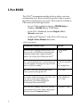
S-PLUS BOOKS
®
The S-PLUS documentation includes books to address your focus
and knowledge level. Review the following table to help you choose
the S-PLUS book that meets your needs. These books are available in
PDF format in the following locations:
•
In your S-PLUS installation directory (SHOME\help on
Windows, SHOME/doc on UNIX/Linux).
•
In the S-PLUS Workbench, from the Help 䉴 S-PLUS
Manuals menu item.
•
In Microsoft Windows , in the S-PLUS GUI, from the
Help 䉴 Online Manuals menu item.
®
®
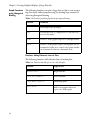
S-PLUS documentation.
Information you need if you...
See the...
Are new to the S language and the S-PLUS GUI,
and you want an introduction to importing data,
producing simple graphs, applying statistical
Getting Started
Guide
®
models, and viewing data in Microsoft Excel .
iv
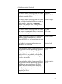
Are a system administrator or a licensed user and
you need guidance licensing your copy of S-PLUS
and/or any S-PLUS module.
S-PLUS licensing Web
site
keys.insightful.com/
Are a new S-PLUS user and need how to use
S-PLUS, primarily through the GUI.
User’s Guide
Are familiar with the S language and S-PLUS, and
you want to use the S-PLUS plug-in, or
customization, of the Eclipse Integrated
Development Environment (IDE).
S-PLUS Workbench
User’s Guide
Have used the S language and S-PLUS, and you
want to know how to write, debug, and program
functions from the Commands window.
Programmer’s Guide
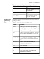
S-PLUS documentation. (Continued)
Information you need if you...
See the...
Are familiar with the S language and S-PLUS, and
you want to extend its functionality in your own
application or within S-PLUS.
Application
Developer’s Guide
Are familiar with the S language and S-PLUS, and
you are looking for information about creating or
editing graphics, either from a Commands
window or the Windows GUI, or using S-PLUSsupported graphics devices.
Guide to Graphics
Are familiar with the S language and S-PLUS, and
you want to use the Big Data library to import and
manipulate very large data sets.
Big Data
User’s Guide
Want to download or create S-PLUS packages for
submission to the Comprehensive S Archival
Network (CSAN) site, and need to know the steps.
Guide to Packages
Are looking for categorized information about
individual S-PLUS functions.
Function Guide
If you are familiar with the S language and S-PLUS,
and you need a reference for the range of statistical
modelling and analysis techniques in S-PLUS.
Volume 1 includes information on specifying
models in S-PLUS, on probability, on estimation
and inference, on regression and smoothing, and
on analysis of variance.
Guide to Statistics,
Vol. 1
If you are familiar with the S language and S-PLUS,
and you need a reference for the range of statistical
modelling and analysis techniques in S-PLUS.
Volume 2 includes information on multivariate
techniques, time series analysis, survival analysis,
resampling techniques, and mathematical
computing in S-PLUS.
Guide to Statistics,
Vol. 2
v
vi
CONTENTS
S-PLUS Books
Chapter 1
Introduction to the Big Data Library
iv
1
Introduction
2
Working with a Large Data Set
3
Size Considerations
7
The Big Data Library Architecture
8
Chapter 2 Census Data Example
21
Introduction
22
Exploratory Analysis
25
Data Manipulation
37
More Graphics
41
Clustering
45
Modeling Group Membership
53
Chapter 3 Creating Graphical Displays
of Large Data Sets
61
Introduction
62
Overview of Graph Functions
63
Example Graphs
69
vii
Contents
Chapter 4
Advanced Programming Information
Introduction
106
Big Data Block Size Issues
107
Big Data String and Factor Issues
113
Storing and Retrieving Large S Objects
119
Increasing Efficiency
121
Appendix: Big Data Library Functions
123
Introduction
124
Big Data Library Functions
125
Index
viii
105
161
INTRODUCTION TO THE BIG
DATA LIBRARY
1
Introduction
2
Working with a Large Data Set
Finding a Solution
No 64-Bit Solution
3
3
5
Size Considerations
Summary
7
7
The Big Data Library Architecture
Block-based Computations
Data Types
Classes
Functions
Summary
8
8
11
14
15
19
1
Chapter 1 Introduction to the Big Data Library
INTRODUCTION
In this chapter, we discuss the history of the S language and large data
sets and describe improvements that the Big Data library presents.
This chapter discusses data set size considerations, including when to
use the Big Data library. The chapter also describes in further detail
the Big Data library architecture: its data objects, classes, functions,
and advanced operations.
To use the Big Data library, you must load it as you would any other
library provided with S-PLUS: that is, at the command prompt, type
library(bigdata).
2
•
To ensure that the library is always loaded on startup, add
library(bigdata) to your SHOME/local/S.init file.
•
Alternatively, in the S-PLUS GUI for Microsoft Windows ,
you can set this option in the General Settings dialog box.
•
In the S-PLUS Workbench, you can set this option in the
S-PLUS section of the Preferences dialog box, available from
the Window menu.
®
Working with a Large Data Set
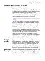
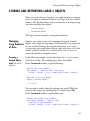
WORKING WITH A LARGE DATA SET
When it was first developed, the S programming language was
designed to hold and manipulate data in memory. Historically, this
design made sense; it provided faster and more efficient calculations
and modeling by not requiring the user’s program to access
information stored on the hard drive. Data size has outstripped the
rate at which RAM size increased; consequently, S program users
could have encountered an error similar to the following:
Problem in read.table: Unable to obtain requested dynamic
memory.
This error occurs because S-PLUS requires the operating system to
provide a block of memory large enough to contain the contents of
the data file, and the operating system responds that not enough
memory is available.
While S-PLUS can access data contained in virtual memory, the
maximum size of data files depends on the amount of virtual memory
available to S-PLUS, which depends in turn on the user’s hardware
and operating system. In typical environments, virtual memory limits
your data file size, and then it returns an out-of-memory error.
Finally, you can also encounter an out-of-memory error after
successfully reading in a large data object, because many S functions
require one or more temporary copies of the source data in RAM for
certain manipulation or analysis functions.
Finding a
Solution
S programmers with large data sets have historically dealt with
memory limitations in a variety of ways. Some opted to use other
applications, and some divided their data into “digestible” batches,
and then recompile the results. For S programmers who like the
flexibility and elegant syntax of the S language and the support
provided to owners of an S-PLUS license, the option to analyze and
model large data sets in S has been a long-awaited enhancement.
Out-of-Memory
Processing
The Big Data library provides this enhancement by processing large
data sets using scalable algorithms and data streaming. Instead of
loading the contents of a large data file into memory, S-PLUS creates a
special binary cache file of the data on the user’s hard disk, and then
3
Chapter 1 Introduction to the Big Data Library
refers to the cache file on disk. This out-of-memory design requires
relatively small amounts of RAM, regardless of the total size of the
data.
Scalable
Algorithms
Although the large data set is stored on the hard drive, the scalable
algorithms of the Big Data library are designed to optimize access to
the data, reading from disk a minimum number of times. Many
techniques require a single pass through the data, and the data is read
from the disk in blocks, not randomly, to minimize disk access times.
These scalable algorithms are described in more detail in the section
The Big Data Library Architecture on page 8.
Data Streaming
S-PLUS operates on the data binary cache file directly, using
“streaming” techniques, where data flows through the application
rather than being processed all at once in memory. The cache file is
processed on a row-by-row basis, meaning that only a small part of
the data is stored in RAM at any one time. It is this out-of-memory
data processing technique that enables S-PLUS to process data sets
hundreds of megabytes, or even gigabytes, in size without requiring
large quantities of RAM.
Data Type
S-PLUS provides the large data frame, an object of class bdFrame. A
big data frame object is similar in function to standard S-PLUS data
frames, except its data is stored in a cache file on disk, rather than in
RAM. The bdFrame object is essentially a reference to that external
file: While you can create a bdFrame object that represents an
extremely large data set, the bdFrame object itself requires very little
RAM.
For more information on bdFrame, see the section Data Frames on
page 11.
S-PLUS also provides time date (bdTimeDate), time span (bdTimeSpan),
and series (bdSeries, bdSignalSeries, and bdTimeSeries) support for
large data sets. For more information, see the section Time Date
Creation on page 157 in the Appendix.
Flexibility
4
The Big Data library provides reading, manipulating, and analyzing
capability for large data sets using the familiar S programming
language. Because most existing data frame methods work in the
same way with bdFrame objects as they do with data.frame objects,
the style of programming is familiar to S-PLUS programmers. Much
existing code from previous versions of S-PLUS runs without
Working with a Large Data Set
modification in the Big Data library, and only minor modifications
are needed to take advantage of the big-data capabilities of the
pipeline engine.
Balancing
Scalability with
Performance
While accessing data on disk (rather than in RAM) allows for scalable
statistical computing, some compromises are inevitable. The most
obvious of these is computation speed. The Big Data library provides
scalable algorithms that are designed to minimize disk access, and
therefore provide optimal performance with out-of-memory data sets.
This makes S-PLUS a reliable workhorse for processing very large
amounts of data. When your data is small enough for traditional
S-PLUS, it’s best to remember that in-memory processes are faster
than out-of-memory processes.
If your data set size is not extremely large, all of the S-PLUS traditional
in-memory algorithms remain available, so you need not compromise
speed and flexibility for scalability when it's not needed.
Metadata
To optimize performance, S-PLUS stores certain calculated statistics as
metadata with each column of a bdFrame object and updates the
metadata every time the data changes. These statistics include the
following:
•
Column mean (for numeric columns).
•
Column maximum and minimum (for numeric and date
columns).
•
Number of missing values in the column.
•
Frequency counts for each level in a categorical column.
Requesting the value of any of these statistics (or a value derived from
them) is essentially a free operation on a bdFrame object. Instead of
processing the data set, S-PLUS just returns the precomputed statistic.
As a result, calculations on columns of bdFrame objects such as the
following examples are practically instantaneous, regardless of the
data set size. For example:
No 64-Bit
Solution
•
mean(census.data$Income)
•
range(census.data$Age)
Are out-of-memory data analysis techniques still necessary in the 64bit age? While 64-bit operating systems allow access to greater
amounts of *virtual* memory, it is the amount of *physical* memory
5
Chapter 1 Introduction to the Big Data Library
that is the primary determinant of efficient operation on large data
sets. For this reason, the out-of-memory techniques described above
are still required to analyze truly large data sets.
64-bit systems increase the amount of memory that the system can
address. This can help in-memory algorithms handle larger problems,
provided that all of the data can be in physical memory. If the data
and the algorithm require virtual memory, page-swapping (that is,
accessing the data in virtual memory on the disk) can have a severe
impact on performance.
With data sets now in the multiple gigabyte range, out-of-memory
techniques are essential. Even on 64-bit systems, out-of-memory
techniques can dramatically outperform in-memory techniques when
the data set exceeds the available physical RAM.
6
Size Considerations
SIZE CONSIDERATIONS
While the Big Data library imposes no predetermined limit for the
number of rows allowed in a big data object or the number of
elements in a big data vector, your computer’s hard drive must
contain enough space to hold the data set and create the data cache.
Given sufficient disk space, the big data object can be created and
processed by any scalable function.
The speed of most Big Data library operations is proportional to the
number of rows in the data set: if the number of rows doubles, then
the processing time also doubles.
The amount of RAM in a machine imposes a predetermined limit on
the number of columns allowed in a big data object, because column
information is stored in the data set’s metadata. This limit is in the
tens of thousands of columns. If you have a data set with a large
number of columns, remember that some operations (especially
statistical modeling functions) increase at a greater than linear rate as
the number of columns increases. Doubling the number of columns
can have a much greater effect than doubling the processing time.
This is important to remember if processing time is an issue.
Summary
By bringing together flexible programming and big-data capability,
S-PLUS is a data analysis environment that provides both rapid
prototyping of analytic applications and a scalable production engine
capable of handling datasets hundreds of megabytes, or even
gigabytes, in size.
In the next section, we provide an overview to the Big Data library
architecture, including data types, functions, and naming
conventions.
7
Chapter 1 Introduction to the Big Data Library
THE BIG DATA LIBRARY ARCHITECTURE
The Big Data library is a separate library from the S-PLUS engine
library. It is designed so that you can work with large data objects the
same way you work with existing S-PLUS objects, such as data frames
and vectors.
Block-based
Computations
Data sets that are much larger than the system memory are
manipulated by processing one “block” of data at a time. That is, if
the data is too large to fit in RAM, then the data will be broken into
multiple data sets and the function will be applied to each of the data
sets. As an example, a 1,000,000 row by 10 column data set of double
values is 76MB in size, so it could be handled as a single data set on a
machine with 256MB RAM. If the data set was 10,000,000 rows by
100 columns, it would be 7.4GB in size and would have to be handled
as multiple blocks.
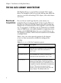
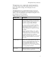
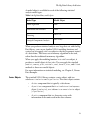
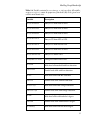
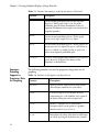
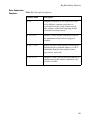
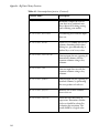
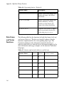
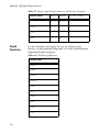
Table 1.1 lists a few of the optional arguments for the function
bd.options that you can use to set limits for caching and for
warnings:
Table 1.1: bd.options block-based computation arguments.
bd.option
8
argument
Description
block.size
The block size (in number of rows), the number
of bytes in the cache to be converted to a
data.frame.
max.convert.bytes
The maximum size (in bytes) of the big data
cache that can be converted to a data.frame.
max.block.mb
The maximum number of megabytes used for
block processing buffers. If the specified block
size requires too much space, the number of rows
is reduced so that the entire buffer is smaller than
this size. This prevents unexpected out-ofmemory errors when processing wide data with
many columns. The default value is 10.
The Big Data Library Architecture
The function bd.options contains other optional arguments for
controlling column string width, display parameters, factor level
limits, and overflow warnings. See its help topic for more
information.
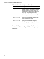
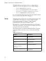
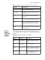
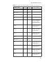
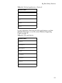
The Big Data library also contains functions that you can use to
control block-based computations. These include the functions in
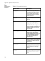
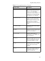
Table 1.2. For more information and examples showing how to use
these functions, see their help topics.
Table 1.2: Block-based computation functions.
Function name
Description
bd.aggregate
Use bd.aggregate to divide a data object into
blocks according to the values of one or more of
its columns, and then apply aggregation
functions to columns within each block.
takes two required arguments:
data, which is the input data set, and by.columns,
which identifies the names or numbers of
columns defining how the input data is divided
into blocks.
bd.aggregate
Optional arguments include columns, which
identifies the names or numbers of columns to
be summarized, and methods, which is a vector
of summary methods to be calculated for
columns. See the help topic for bd.aggregate for
a list of the summary methods you can specify
for methods.
bd.block.apply
Run an S-PLUS script on blocks of data, with
options for reading multiple input datasets and
generating multiple output data sets, and
processing blocks in different orders. See the
help topic for bd.block.apply for a discussion on
processing multiple data blocks.
bd.by.group
Apply the specified S-PLUS function to multiple
data blocks within the input dataset.
9
Chapter 1 Introduction to the Big Data Library
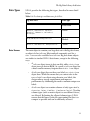
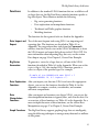
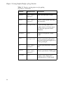
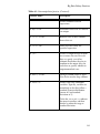
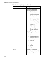
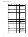
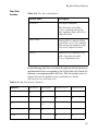
Table 1.2: Block-based computation functions. (Continued)
Function name
Description
bd.by.window
Apply the specified S-PLUS function to multiple
data blocks defined by a moving window over
the input dataset. Each data block is converted to
a data.frame, and passed to the specified
function. If one of the data blocks is too large to
fit in memory, an error occurs.
bd.split.by.group
Divide a dataset into multiple data blocks, and
return a list of these data blocks.
bd.split.by.window
Divide a dataset into multiple data blocks
defined by a moving window over the dataset,
and return a list of these data blocks.
For a detailed discussion on advanced topics, such as block size issues
and increasing efficiency, see Chapter 4, Advanced Programming
Information.
10
The Big Data Library Architecture
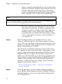
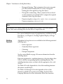
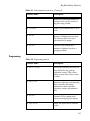
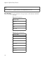
Data Types
S-PLUS provides the following data types, described in more detail
below:
Table 1.3: New data types and data names for S-PLUS.
Big Data class
Data type
bdFrame
Data frame
bdVector, bdCharacter, bdFactor,
bdLogical, bdNumeric, bdTimeDate,
bdTimeSpan
Vector
bdLM, bdGLM, bdPrincomp, bdCluster
Models
bdSeries, bdTimeSeries, bdSignalSeries
Data Frames
Series
The main object to contain your large data set is the big data frame,
an object of class bdFrame. Most methods commonly used for a
data.frame are also available for a bdFrame. Big data frame objects
are similar to standard S-PLUS data frames, except in the following
ways:
•
A bdFrame object stores its data on disk, while a data.frame
object stores its data in RAM. As a result, a bdFrame object has
a much smaller memory footprint than a data.frame object.
•
A bdFrame object does not have row labels, as a data.frame
object does. While this means that you cannot refer to the
rows of a bdFrame object using character row labels, this
design reduces storage requirements and improves
performance by eliminating the need to maintain unique row
labels.
•
A bdFrame object can contain columns of only types double,
character, factor, timeDate, timeSpan or logical. No other
column types (such as matrix objects or user-defined classes)
are allowed. By limiting the allowed column types, S-PLUS
ensures that the binary cache file representing the data is as
compact as possible and can be efficiently accessed.
11
Chapter 1 Introduction to the Big Data Library
•
The print function works differently on a bdFrame object than
it does for a data frame. It displays only the first few rows and
columns of data instead of the entire data set. This design
prevents accidentally generating thousands of pages of output
when you display a bdFrame object at the command line.
Note
You can specify the numbers of rows and columns to print using the bd.options function. See
bd.options in the S-PLUS Language Reference for more information.
•
Vectors
The summary function works differently on a bdFrame object
than it does for a data frame. It calculates an abbreviated set
of summary statistics for numeric columns. This design is for
efficiency reasons: summary displays only statistics that are
precalculated for each column in the big data object, making
summary an extremely fast function, even when called on a
very large data set.
The S-PLUS Big Data library also introduces bdVector and six
subclasses, which represent new vector types to support very long
vectors. Like a bdFrame object, the big vector object stores data out-ofmemory as a cache file on disk, so you can create very long big vector
objects without needing a lot of RAM.
You can extract an individual column from a bdFrame object (using
the $ operator) to create a large vector object. Alternatively, you can
generate a large vector using the functions listed in Table A.3 in the
Appendix. Like bdFrame objects, the actual data is stored out of
memory as a cache file on disk, so you can create very long big vector
objects without worrying about fitting them into RAM. You can use
standard vector operations, such as selections and mathematical
operations, on these data types. For example, you can create new
columns in your data set, as follows:
census.data$adjusted.income <- log(census.data$income census.data$tax)
Models
12
S-PLUS Big Data library provides scalable modeling algorithms to
process big data objects using out-of-memory techniques. With these
modeling algorithms, you can create and evaluate statistical models
on very large data sets.
The Big Data Library Architecture
A model object is available for each of the following statistical
analysis model types.
Table 1.4: Big Data library model objects.
Model Type
Model Object
Linear regression
bdLm
Generalized linear models
bdGlm
Clustering
bdCluster
Principal Components Analysis
bdPrincomp
When you perform statistical analysis on a large data set with the Big
Data library, you can use familiar S-PLUS modeling functions and
syntax, but you supply a bdFrame object as the data argument, instead
of a data frame. This forces out-of-memory algorithms to be used,
rather than the traditional in-memory algorithms.
When you apply the modeling function lm to a bdFrame object, it
produces a model object of class bdLm. You can apply the standard
predict, summary, plot, residuals, coef, formula, anova, and fitted
methods to these new model objects.
For more information on statistical modeling, see Chapter 2, Census
Data Example.
Series Objects
The standard S-PLUS library contains a series object, with two
subclasses: timeSeries and signalSeries. The series object contain:
•
A data component that is typically a data frame.
•
A positions component that is a timeDate or timeSequence
object (timeSeries), or a bdNumeric or numericSeries object
(signalSeries).
•
A units component that is a character vector with
information on the units used in the data columns.
13
Chapter 1 Introduction to the Big Data Library
The Big Data library equivalent is a bdSeries object with two
subclasses: bdTimeSeries and bdSignalSeries. They contain:
•
A data component that is a bdFrame.
•
A positions component that is a bdTimeDate object
(bdTimeSeries), or bdNumeric object (bdSignalSeries).
•
A units component that is a character vector.
For more information about using large time series objects and their
classes, see the section Time Classes on page 17.
Classes
The Big Data library follows the same object-oriented design as the
standard S-PLUS Sv4 design. For a review of object-oriented
programming concepts, see Chapter 8, Object-Oriented
Programming in S-PLUS in the Programmer’s Guide.
Each object has a class that defines methods that act on the object.
The library is extensible; you can add your own objects and classes,
and you can write your own methods.
The following classes are defined in the Big Data library. For more
information about each of these classes, see their individual help
topics.
Table 1.5: Big Data classes.
Class(es)
Description
bdFrame
Big data frame
bdLm, bdGlm, bdCluster, bdPrincomp
Rich model objects
bdVector
Big data vector
bdCharacter, bdFactor, bdLogical,
Vector type subclasses
bdNumeric, bdTimeDate,
bdTimeSpan
bdTimeSeries, bdSignalSeries
14
Series objects
The Big Data Library Architecture
Functions
In addition to the standard S-PLUS functions that are available to call
on large data sets, the Big Data library includes functions specific to
big data objects. These functions include the following.
•
Big vector generating functions
•
Data exploration and manipulation functions.
•
Traditional and Trellis graphics functions.
•
Modeling functions.
The functions for these general tasks are listed in the Appendix.
Data Import and Two of the most frequent tasks using S-PLUS are importing and
exporting data. The functions are described in Table A.1 in
Export
Appendix. You can perform these tasks from the Commands
window, from the Console view in the S-PLUS Workbench, or from
the S-PLUS import and export dialog boxes in the S-PLUS GUI. For
more information about importing large data sets, see the section
Data Import on page 25 in Chapter 2, Census Data Example.
Big Vector
Generation
To generate a vector for a large data set, call one of the S-PLUS
functions described in Table A.3 in the Appendix. When you set the
bigdata flag to TRUE, the standard S-PLUS functions generate a
bdVector object of the specified type. For example:
# sample of size 2000000 with mean 10*0.5 = 5
rbinom(2000000, 10, 0.5, bigdata = T)
Data Exploration After you import your data into S-PLUS and create the appropriate
objects, you can use the functions described in Table A.4 in the
Functions
Appendix. to compare, correlate, crosstabulate, and examine
univariate computations.
Data
Manipulation
Functions
After you import and examine your data in S-PLUS, you can use the
data manipulation functions to append, filter, and clean the data. For
an overview of these functions, see Table A.5 in the Appendix. For a
more in-depth discussion of these functions, see the section Data
Manipulation on page 37 in Chapter 2, Census Data Example.
Graph Functions
The Big Data library supports graphing large data sets intelligently,
using the following techniques to manage many thousands or millions
of data points:
15
Chapter 1 Introduction to the Big Data Library
•
Hexagonal binning. (That is, functions that create one point
per observation in standard S-PLUS create a hexagonal
binning plot when applied to a big data object.)
•
Plot-specific summarizing. (That is, functions that are based
on data summaries in standard S-PLUS compute the required
summaries from a big data object.)
•
Preprocessing data, using table, tapply, loess, or aggregate.
•
Preprocessing using interp or hist2d.
Note
The Windows GUI editable graphics do not support big data objects. To use these graphics,
create a data frame containing either all of the data or a sample of the data.
For a more detailed discussion of graph functions available in the Big
Data library, see Chapter 3, Creating Graphical Displays of Large
Data Sets.
Modeling
Functions
Algorithms for large data sets are available for the following statistical
modeling types:
•
Linear regression.
•
Generalized linear regression.
•
Clustering.
•
Principal components.
See the section Models on page 12 for more information about the
modeling objects.
If the data argument for a modeling function is a big data object, then
S-PLUS calls the corresponding big data modeling function. The
modeling function returns an object with the appropriate class, such
as bdLm.
See Table A.12 in the Appendix for a list of the modeling functions
that return a model object.
See Tables A.10 through A.13 in the Appendix for lists of the
functions available for large data set modeling. See the S-PLUS
Language Reference for more information about these functions.
16
The Big Data Library Architecture
Formula operators
The Big Data library supports using the formula operators+, -, *, :,
%in%, and /.
Time Classes
The following classes support time operations in the Big Data library.
See the Appendix for more information.
Table 1.6: Time classes.
Time Series
Operations
Time and Date
Operations
Class name
Comment
bdSignalSeries
A bdSignalSeries object from
positions and data
bdTimeDate
A bdVector class
bdTimeSeries
See the section Time Series
Operations for more information.
bdTimeSpan
A bdVector class
Time series operations are available through the bdTimeSeries class
and its related functions. The bdTimeSeries class supports the same
methods as the standard S-PLUS library’s timeSeries class. See the
S-PLUS Language Reference for more information about these classes.
•
When you create a time object using timeSeq, and you set the
bigdata argument to TRUE, then a bdTimeDate object is
created.
•
When you create a time object using timeDate or
timeCalendar, and any of the arguments are big data
then a bdTimeDate object is created.
objects,
See Table A.14 in the Appendix.
Note
always assumes the time as Greenwich Mean Time (GMT); however, S-PLUS stores
no time zone with an object. You can convert to a time zone with timeZoneConvert, or specify the
zone in the bdTimeDate constructor.
bdTimeDate
17
Chapter 1 Introduction to the Big Data Library
Time Conversion
Operations
To convert time and date values, apply the standard S-PLUS time
conversion operations to the bdTimeDate object, as listed in Table
A.14 in the Appendix.
Matrix
Operations
The Big Data library does not contain separate equivalents to matrix
and data.frame.
S-PLUS matrix operations are available for bdFrame objects:
•
matrix algebra ( +, -, /, *, !, &, |, >, <, ==, !=, <=, =>, %%, %/%)
•
matrix multiplication (%*%)
•
Crossproduct (crossprod)
In algebraic operations, the operators require the big data objects to
have appropriately-corresponding dimensions. Rows or columns are
not automatically replicated.
Basic algebra
You can perform addition, subtraction, multiplication, division,
logical (!, &, and |), and comparison (>, <, =, !=, <=, >=) operations
between:
•
A scalar and a bdFrame.
•
Two bdFrames of the same dimension.
•
A bdFrame and a single-row bdFrame with the same number of
columns.
•
A bdFrame and a single-column bdFrame with the same
number of rows.
The library also offers support for element-wise +, -, *, /, and matrix
multiplication (%*%).
Matrix multiplication is available for two bdFrames with the
appropriate dimensions.
Cross Product Function
When applied against two bdFrames, the cross product function,
crossprod, returns a bdFrame that is the cross product of the given
bdFrames. That is, it returns the matrix product of the transpose of the
first bdFrame with the second.
18
The Big Data Library Architecture
Summary
In this section, we’ve provided an overview to the Big Data library
architecture, including the new data types, classes, and functions that
support managing large data sets. For more detailed information and
lists of functions that are included in the Big Data library, see the
Appendix: Big Data Library Functions.
In the next chapter, we provide examples for working with data sets
using the types, classes, and functions described in this chapter.
19
Chapter 1 Introduction to the Big Data Library
20
CENSUS DATA EXAMPLE
2
Introduction
Problem Description
Data Description
22
22
22
Exploratory Analysis
Data Import
Data Preparation
Tabular Summaries
Graphics
25
25
27
31
32
Data Manipulation
Stacking
Variable Creation
Factors
37
37
38
40
More Graphics
41
Clustering
Data Preparation
K-Means Clustering
Analyzing the Results
45
45
46
47
Modeling Group Membership
Building a Model
Summarizing the Fit
Characterizing the Group
53
57
58
58
21
Chapter 2 Census Data Example
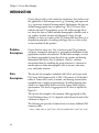
INTRODUCTION
Census data provides a rich context for exploratory data analysis and
the application of both unsupervised (e.g., clustering) and supervised
(e.g., regression) statistical learning models. Furthermore the data sets
(in their unaggragated state) are quite large. The US Census 2000
estimates the total US population at over 281 million people. In its
raw form, the data set (which includes demographic variables such as
age, gender, location, income and education) is huge. For this
example, we focus on a subset of the US Census data that allows us to
demonstrate principles of working with large data on a data set that
we have included in the product.
Problem
Description
Census data has many uses. One of interest to the US government
and many commercial enterprises is geographical distribution of sub
populations and their characteristics. In this initial example, we look
for distinct geographical groups based on age, gender and housing
information (data that is easy to obtain in a survey), and then
characterize them by modeling the group structure as a function of
much harder-to-obtain demographics such as income, education,
race, and family structure.
Data
Description
The data for this example is included with S-PLUS and is part of the
US Census 2000 Summary File 3 (SF3). SF3 consists of 813 detailed
tables of Census 2000 social, economic, and housing characteristics
compiled from a sample of approximately 19 million housing units
(about 1 in 6 households) that received the Census 2000 long-form
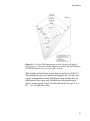
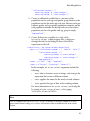
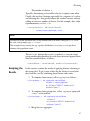
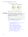
questionnaire. The levels of aggregation for SF3 data is depicted in
Figure 2.1.
The data for this example is the summary table aggregated by Zip
Code Tabulation Areas (ZCTA5) depicted as the left-most branch of the
schematic in Figure 2.1.
The following site provides download access to many additional SF3
summary tables:
http://www.census.gov/Press-Release/www/2002/sumfile3.html
22
Introduction
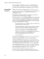
Figure 2.1: US Census 2000 data grouping hierarchy schematic with implied
aggregation levels. The data used in this example comes from the Zip Code Tabulation
Area (ZCTA) depicted at the far left side of the schematic.
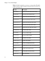
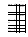
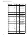
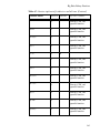
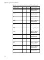
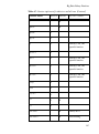
The variables included in the census data set are listed in Table 2.1.
They include the zip code, latitude and longitude for each zip code
region, and population counts. Population counts include the total
population for the region and a breakdown of the population by
gender and age group: Counts of males and females for ages 0 - 5, 5 10, ..., 80 - 85, and 85 or older.
23
Chapter 2 Census Data Example
Table 2.1: Variable descriptions for the census data example.
Variable(s)
New Variable
Name(s)
Description
ZCAT5
zipcode
five-number zip code
INTPT.LAT
lat
Interpolated latitude
INTPT.LON
long
Interpolated longitude
P008001
popTotal
Total population
M.00 - M.85
male.00 male.85
Male population by age group:
0 - 4 years, 5 - 9 years, and so
on.
F.00 - F.85
female.00 female.85
Female population by age
group: 0 - 4 years, 5 - 9 years,
and so on.
H007001
housingTotal
Total housing units
H007002
own
Owner occupied
H007003
rent
Renter occupied
A script file can be downloaded from Insightful’s Support site that
contains all the commands used in this chapter:
www.insightful.com/support/downloads/examples/
new.census.demo.ssc
If you want to build the cluster model starting on page 57, you also
need to download the following object:
www.insightful.com/support/downloads/examples/
censusDemogr.sdd
Then run data.restore("C:/test/censusDemogr.sdd") to restore it
for use in S-PLUS, where C:/test is an example download folder.
24
Exploratory Analysis
EXPLORATORY ANALYSIS
Data Import
The data is provided as a comma-separated text file ( .csv format).
The file is located in the SHOME location (by default your
installation directory) in /samples/bigdata/census/census.csv.
As mentioned on the previous page, you can also download an
analysis script named new.census.demo.ssc to execute the
commands referenced in this chapter.
Reading big data is identical to what you are familiar with in previous
versions of S-PLUS with one exception: an additional argument to
specify that the data object created is stored as a big data (bd) object.
> census <- importData(paste(getenv("SHOME"),
"/samples/bigdata/census/census.csv", sep=""),
stringsAsFactors=F, bigdata=T)
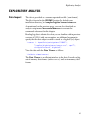
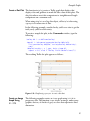
View the data with the Data Viewer as follows:
> bd.data.viewer(census)
The Data Viewer is an efficient interface to the data. It works on big
out-of-memory data frames (such as census) and on in-memory data
frames.
25
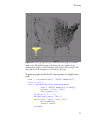
Chapter 2 Census Data Example
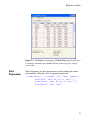
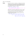
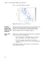
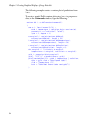
Figure 2.2: Viewing big data objects is done with the Data Viewer.
The Data View page (Figure 2.2) of the Data Viewer lists all rows
and all variables in a scrollable window plus summary information at
the bottom, including the number of rows, the number of columns,
and a count of the number of different types of variables (for
example, a numeric, factor). From the summary information, we see
that census has 33,178 rows.
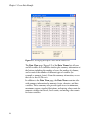
In addition to the Data View page, the Data Viewer contains tabs
with summary information for numeric, factor, character, and date
variables. These summary tabs provide quick access to minimums,
maximums, means, standard deviations, and missing value counts for
numeric variables and levels, level counts, and missing value counts
for factor variables.
26
Exploratory Analysis
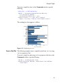
Figure 2.3: The Numeric summary page of the Data Viewer provides quick access
to minimum, maximum, mean, standard deviation, and missing value count for
numeric data.
Data
Preparation
Before beginning any data preparation, start by making the names
more intuitive using the names assignment expression:
> names(census) <- c("zipcode", "lat", "long", "popTotal",
paste("male", seq(0, 85, by = 5), sep = "."),
paste("female", seq(0, 85, by = 5), sep = "."),
"housingTotal", "own", "rent")
27
Chapter 2 Census Data Example
The row names are shown in Table 2.1, along with the original
names.
Note
The S-PLUS expression paste("male", seq(0, 85, by = 5), sep = ".") creates a sequence of 18
variable names starting with male.0 and ending with male.85. The call to seq generates a
sequence of integers from 0 to 85 incremented by 5, and the call to paste pastes together the
string “male” with the sequence of integers separated with a period (.).
A summary of the data now is:
> summary(census)
zipcode
Length:
33178
Class:
Mode:character
popTotal
Min.:
0.000
Mean: 8596.977
Max.:144024.000
.
.
.
lat
Min.:17962234
Mean:38830389
Max.:71299525
male.0
Min.:
0.0000
Mean: 298.5727
Max.:6247.0000
long
Min.:-176636755
Mean: -91084343
Max.: -65292575
male.5
Min.:
0.000
Mean: 322.822
Max.:6115.000
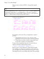
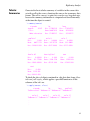
From summary of the census data, you might notice a couple of
problems:
1. The population total (popTotal) has some zero values,
implying that some zip codes regions contain no population.
2. The zip codes are stored as character strings which is odd
because they are defined as five-digit numbers.
To remove the zero-population zip codes you can do it the you
typically would when working with data frames:
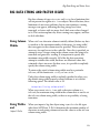
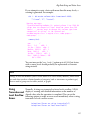
> census <- census[census[, "popTotal"] > 0, ]
However, there is a more efficient way. Notice that the example
above (finding rows with non-zero population counts) implies two
passes through the data. The first pass extracts the popTotal column
and compares it (row by row) with the value of zero. The second pass
28
Exploratory Analysis
removes the bad popTotal rows. If your data is very large, using
subscripting and nested function calls can result in a prohibitively
lengthy execution time.
A more efficient “big data” way to remove rows with no population is
to use the bd.filter.rows function available in the Big Data library
in S-PLUS. bd.filter.rows has two required arguments:
1. data: the big data object to be filtered.
2. expr: an expression to evaluate. By default, the expression
must be valid, based on the rules of the row-oriented
Expression Language. For more details on the expression
language, see the help file for ExpressionLanguage.
Note
If you are familiar with the S-PLUS language, the Excel formula language, or another
programming language, you will find the row-oriented Expression Language natural and easy to
use. An expression is a combination of constants, operators, function calls, and references to
columns that returns a single value when evaluated
For our example, the expression is simply popTotal > 0, which you
pass as a character string to bd.filter.rows. The more efficient way
to filter the rows is:
> census <- bd.filter.rows(census, expr= "popTotal >
0")
29
Chapter 2 Census Data Example
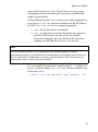
Using the row-oriented Expression Language with bd.filter.rows
results in only one pass through the data, so the computation time will
usually be reduced to about half the execution time of the previouslydescribed S-PLUS expression. Table 2.2 displays additional examples
of row-oriented expressions.
Table 2.2: Some examples of the row-oriented Expression Language.
Expression
Description
age > 40 & gender == “F”
All rows with females greater than
40 years of age.
Test != “Failed”
All rows where Test is not equal to
“Failed”.
Date > 6/30/04
All rows with Date later than
6/30/04.
voter == “Dem” | voter == “Ind”
All rows where voter is either
democrat or independent.
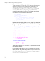
Now, remove the cases with bad zip codes by using the regular
expression function, regexpr, to find the row indices of zip codes that
have only numeric characters:
> census <- bd.filter.rows(census,
"regexpr('^[0-9]+$', zipcode)>0",
row.language=F)
Notes
30
•
The call to the regexpr function finds all zip codes that have only integer characters in
them. The regular expression “^[0-9]+$” produces a search for strings that contain only
the characters 0, 1, 2, ..., 9. The ^ character indicates starting at the beginning of
the string, the $ character indicates continuing to the end of the string and the + symbol
implies any number of characters from the set {0, 1, 2,..., 9}.
•
The call to bd.filter.rows specified the optional argument, row.language=F. This
argument produces the effect of using the standard S-PLUS expression language, rather
than the row-oriented Expression Language designed for row operations on big data.
Exploratory Analysis
Tabular
Summaries
Generate the basic tabular summary of variables in the census data
set with a call to the summary function, the same as for in-memory data
frames. The call to summary is quite fast, even for very large data sets,
because the summary information is computed and stored internally
at the time the object is created.
> summary(census)
zipcode
Length:
32165
Class:
Mode:character
popTotal
Min.:
1.000
Mean: 8867.729
Max.:144024.000
.
.
.
female.85
Min.:
0.00000
Mean: 92.77398
Max.:2906.00000
lat
Min.:17964529
Mean:38847016
Max.:71299525
long
Min.:-176636755
Mean: -91103295
Max.: -65292575
male.0
Min.:
0.0000
Mean: 307.9759
Max.:6247.0000
male.5
Min.:
0.0000
Mean: 332.9889
Max.:6115.0000
housingTotal
Min.:
0.000
Mean: 3318.558
Max.:61541.000
own
Min.:
0.000
Mean: 2199.168
Max.:35446.000
rent
Min.:
0.000
Mean: 1119.391
Max.:40424.000
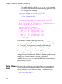
To check the class of objects contained in a big data data frame (class
bdFrame), call sapply, which applies a specified function to all the
columns of the bdFrame.
> sapply(census, class)
zipcode
lat
long
popTotal
"bdCharacter" "bdNumeric" "bdNumeric" "bdNumeric"
male.0
male.5
male.10
male.15
"bdNumeric" "bdNumeric" "bdNumeric" "bdNumeric"
.
.
.
31
Chapter 2 Census Data Example
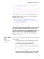
Generate age distribution tables with the same operations you use for
in-memory data. Multiply column means by 100 to convert to a
percentage scale and round the output to one significant digit:
> ageDist <colMeans(census[, 5:40] / census[, "popTotal"]) * 100
> round(matrix(ageDist,
nrow = 2,
byrow = T,
dimnames = list(c("Male", "Female"),
seq(0, 85, by=5))), 1)
numeric matrix: 2 rows, 18 columns.
0
5 10 15 20 25 30 35 40 45 50 55
Male 3.2 3.6 3.8 3.8 2.9 2.9 3.2 3.9 4.1 3.8 3.3 2.7
Female 3.0 3.4 3.6 3.4 2.7 2.8 3.2 3.9 4.0 3.7 3.3 2.7
60 65 70 75 80 85
Male 2.3 2.0 1.7 1.3 0.8 0.5
Female 2.3 2.1 2.0 1.7 1.2 1.1
Graphics
You can plot the columns of a bdFrame in the same manner as you do
for regular (in-memory) data frames:
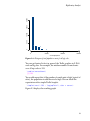
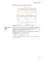
> hist(census$popTotal)
will produce a histogram of total population counts for all zip codes.
Figure 2.4 displays the result.
32
0
5000
10000
15000
20000
Exploratory Analysis
0
50000
100000
150000
census$popTotal
Figure 2.4: Histogram of total population counts for all zip codes.
You can get fancier. In fact, in general, the Trellis graphics in S-PLUS
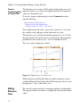
work on big data. For example, the median number of rental units
over all zip codes is 193:
> median(census$rent)
[1] 193
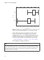
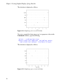
You would expect that, if the number of rental units is high (typical of
cities), the population would likewise be high. We can check this
expectation with a simple Trellis boxplot:
> bwplot(rent > 193 ~ log(popTotal), data = census)
Figure 2.5 displays the resulting graph.
33
Chapter 2 Census Data Example
rent > 193
TRUE
FALSE
0
2
4
6
8
10
12
log(popTotal)
Figure 2.5: Boxplots of the log of popTotal for the number of rental units above and
below the median, showing higher populations in areas with more rental units.
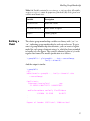
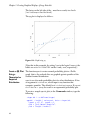
You can address the question of population size relative to the
number of rental units in a more general way by examining a
scatterplot of popTotal vs. rent. Call the Trellis function xyplot for
this. Take logs (after adding 0.5 to eliminate zeros) of each of the
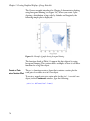
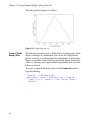
variables to rescale the data so the relationship is more exposed:
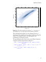
> xyplot(log(popTotal) ~ log(rent + 0.5), data = census)
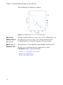
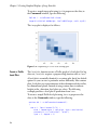
The resulting plot is displayed in Figure 2.6.
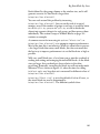
Note
The default scatterplot for big data is a hexbin scatterplot. The color shading of the hexagonal
“points” indicate the number of observations in that region of the graph. For the darkest shaded
hexagon in the center of the graph, over 800 zip codes are represented, as indicated by the
legend on the right side of the graph.
34
Exploratory Analysis
12
800
700
10
600
log(popTotal)
8
500
6
400
4
300
200
2
100
0
1
0
2
4
6
8
10
log(rent + 0.5)
Figure 2.6: This hexbin scatterplot of log(popTotal) vs. log(rent+0.5)
shows population sizes increasing with the increasing number of rental units.
The result displayed in Figure 2.6 is not surprising; however, it
demonstrates the straightforward use of known functions on big data
objects. This example continues with Trellis graphics with
conditioning in the following sections.
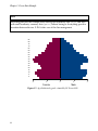
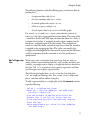
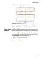
The age distribution table created in the section Tabular Summaries
on page 31 produces the plot shown in Figure 2.7:
> bars <- barplot(rbind(ageDist[1:18], -ageDist [19:36]),
horiz=T)
> mtext(c("Female", "Male"), side = 1, line = 3, cex = 1.5,
at = c(-2, 2))
> axis(2, at = bars, labels = seq(0, 85, by = 5),
ticks =F)
35
Chapter 2 Census Data Example
Note
In creating this plot, the example starts with big out-of-memory data (census) and ends
with small in-memory summary data (ageDist) without having to do anything special to
transition between the two. S-PLUS takes care of the data management.
85
80
75
70
65
60
55
50
45
40
35
30
25
20
15
10
5
0
-4
-2
Female
0
2
Male
Figure 2.7: Age distribution by gender estimated by US Census 2000.
36
4
Data Manipulation
DATA MANIPULATION
The census data contains raw population counts by gender and age;
however, the counts for different genders and ages are in different
columns. To compare them more easily, stack the columns end to
end and create factors for gender and age. Start with the stacking
operation.
Stacking
The bd.stack function provides the needed stacking operation. Stack
all the population counts for males and females for all ages with one
call to bd.stack:
> censusStack <- bd.stack(census,
columns = 5:40,
replicate = c(1:4, 41:43),
stack.column.name = "pop",
group.column.name = "sexAge")
Table 2.3 lists the arguments to bd.stack.
Table 2.3: Arguments to bd.stack.
Argument Name
Description
data
Input data set, a bdFrame or data.frame.
columns
Names or numbers of columns to be stacked.
replicate
Names or numbers of columns to be replicated.
stack.column.name
Name of new stacked column.
group.column.name
Name of an additional group column to be
created in the output data set. In each output
row, the group column contains the name of the
original column that contained the data value in
the new stacked column.
The first few rows of the resulting data are listed below. Notice the
values for the sexAge variable are the names of the columns that were
stacked.
37
Chapter 2 Census Data Example
> censusStack
** bdFrame: 1150236 rows, 9 columns **
zipcode
lat
long popTotal housingTotal
own rent
1
601 18180103 -66749472
19143
5895 4232 1663
2
602 18363285 -67180247
42042
13520 10903 2617
3
603 18448619 -67134224
55592
19182 12631 6551
4
604 18498987 -67136995
3844
1089
719 370
5
606 18182151 -66958807
6449
2013 1463 550
pop sexAge
1 712 male.0
2 1648 male.0
3 2049 male.0
4 129 male.0
5 259 male.0
... 1150231 more rows ...
Notice that the census data started with a little over 33,000 rows.
Now, after stacking, there are over 1.15 million rows.
Variable
Creation
Now create the sex and age factors. There are several ways to do this,
but the most computationally efficient way for large data is to use the
bd.create.columns function, along with the row-oriented expression
language. Before starting, notice that the column names for the
stacked columns (male.0, male.5, ..., female.80, female.85) can be
separated into male and female groups simply by the number of
characters in their names. All male names have seven or fewer
characters and all female names have eight or more characters.
Therefore, by checking the number of characters in the string, you
can determine whether the value should be “male” or “female”. Here
is an example of the row-oriented Expression Language:
" ifelse(nchar(sexAge) > 7, 'female', 'male' "
Notice the use of a single quote, ‘, to embed a quote within a quote.
To create the age variable is a little harder. You must subset the string
differently, depending on whether the value of sexAge corresponds to
a male or female.
1. For males, extract from the sixth character to the end, and for
females, extract from the eighth character to the end. The
row-oriented expression language follows:
38
Data Manipulation
" ifelse(nchar(sexAge) > 7,
substring(sexAge, 8, nchar(sexAge)),
substring(sexAge, 6, nchar(sexAge))) "
2. Create an additional variable that is a measure of the
population size for each age and gender group relative to the
population size for the entire zip code area. Because each row
contains gender and age specific population estimates and the
total population estimate for that zip code area, the relative
population size for each gender and age group is simply
"pop/popTotal"
3. Create all three new variables in a single call to
bd.create.columns (which requires only a single pass
through the data) by including all three of the above
expressions in the call.
> censusStack <- bd.create.columns(censusStack,
exprs = c("ifelse(nchar(sexAge) > 7, 'female', 'male')",
"ifelse(nchar(sexAge) > 7,
substring(sexAge, 8, nchar(sexAge)),
substring(sexAge, 6, nchar(sexAge)))" ,
"pop/popTotal"),
names. = c("sex", "age", "popProp"),
types = c("factor", "character", "numeric"))
In this example, bd.create.columns arguments include the
following:
takes a character vector of strings; each string is the
expression that creates a different column.
•
exprs
•
names
supplies the names for the newly-created columns.
•
types
specifies the type of data in the resulting column.
For more information on bd.create.columns, see its help file
by typing help(bd.create.columns), or by typing
?bd.create.columns in S-PLUS.
Note
The age column in the call to bd.create.columns is stored as a character column so we have
more control when creating an age factor. A discussion of this is included in the next section
Factors.
39
Chapter 2 Census Data Example
Factors
In the previous section, we created age as a character vector, because
when bd.create.columns creates factors, it establishes levels as the
set of alphabetically sorted unique values in the column. The levels are
not arranged numerically. In the example output below, notice the
placement of the “5” between “45” and “50”.
> levels(factor(censusStack[, “age”]))
[1] "0" "10" "15" "20" "25" "30" "35" "40" "45" "5"
[12] "55" "60" "65" "70" "75" "80" "85"
"50"
When S-PLUS creates tables or graphics that use the levels as labels,
the order is as the levels are listed, rather than in numerical order.
To control the order of the levels of a factor, call the bdFactor
function directly and state explicitly the order for the levels. For
example, using the census data:
> censusStack[, "age"] <- bdFactor(censusStack[, "age"],
levels = c("0", "5", "10", "15", "20", "25",
"30", "35", "40", "45", "50", "55",
"60", "65", "70", "75", "80", "85"))
40
More Graphics
MORE GRAPHICS
The data is now prepared to allow more interesting graphics. For
example, create an age distribution plot conditional on gender (Figure
2.8) with the following call to bwplot, a Trellis graphic function:
> bwplot(age ~ log(popProp + 0.00001) | sex,
data = censusStack)
Note
0.00001 is added to the population proportions to avoid taking the log of zero.
-10
female
-8
-6
-4
-2
0
male
85
80
75
70
65
60
55
age
50
45
40
35
30
25
20
15
10
5
0
-10
-8
-6
-4
-2
0
log(popProp + 1e-005)
Figure 2.8: Boxplots of logged relative population numbers by age and sex.
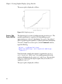
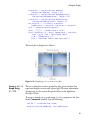
The following call to bwplot creates a plot (Figure 2.9) of logged
relative population numbers by age and whether the zip code area
contains more than the median number of rental units:
> bwplot(age ~ log(popProp + 0.00001) | rent > 193,
data = censusStack)
41
Chapter 2 Census Data Example
Note the span of the boxes for 80 and older when there are fewer
than the median number of rental units, implying that the population
numbers for this group drops dramatically in some areas where there
few rental units.
-10
FALSE
-8
-6
-4
-2
0
TRUE
85
80
75
70
65
60
55
age
50
45
40
35
30
25
20
15
10
5
0
-10
-8
-6
-4
-2
0
log(popProp + 1e-005)
Figure 2.9: Boxplots of logged relative population numbers by age and rent>193.
Another interesting plot is of the zip code area centers in units of
latitude and longitude. Highly populated areas show a higher density
of zip code numbers; therefore, they show greater density in the
hexbin scatterplot. First, however, notice that the scale of lat and
long is off by a factor of 1,000,000. The lat variable should be in the
range of 20 to 70 and long should be in the range of -60 to -180. So
first rescale these variables by a call to bd.create.columns.
> summary(census[, c("lat", "long")])
lat
long
Min.:17964529
Min.:-176636755
Mean:38851462
Mean: -91044543
Max.:71299525
Max.: -65292575
Even more efficient, requiring no passes through the data:
42
More Graphics
> summary(census)[, c("lat", "long")]
Because the summary is stored in metadata, it does not have to be
computed. The first form creates a two-column big data object, and
then gets the summary from that object.
To rescale lat and long simultaneously, use the following
expressions:
"lat/1e6", "long/1e6"
Use the original data set census, rather than censusStack, because
census has just one row per zip code.
> census <- bd.create.columns(census,
exprs=c("lat/1.e6", "long/1.e6"),
names=c("lat","long"))
The values of lat and long are now scaled appropriately:
> summary(census[, c("lat", "long")])
lat
long
Min.:17.96453
Min.:-176.63675
Mean:38.85146
Mean: -91.04454
Max.:71.29953
Max.: -65.29257
Or, more efficiently:
> summary(census)[, c("lat", "long")]
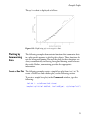
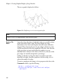
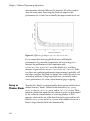
Now produce the plot with a simple call to xyplot.
43
Chapter 2 Census Data Example
> xyplot(lat ~ long, data = census)
70
1200
60
1000
50
lat
800
40
600
400
30
200
20
1
-180
-160
-140
-120
-100
-80
-60
long
Figure 2.10: Hexbin scatterplot of latitudes and longitudes. Zip codes are denser
where populations are denser, so this plot displays relative population densities.
44
Clustering
CLUSTERING
This section applies clustering techniques to the census data to find
sub populations (collections of zip code areas) with similar age
distributions. The section Modeling Group Membership develops
models that characterize the subgroups we find by clustering.
Data
Preparation
The section Tabular Summaries computed the average age distribution
across all zip code areas by age and gender, depicted in Figure 2.7.
Next, group zip-code areas by age distribution characteristics, paying
close attention to those that deviate from the national average. For
example, age distributions in areas with military bases, typically
dominated by young adult single males without children, should
stand out from the national average.
Unusual populations are most noticeable if the population
proportions (previously computed as pop/popTotal by age and
gender) are normalized by the national average. One way to
normalize is to divide population proportions in each age and gender
group by the national average for each age and gender group. The
(odds) ratio represents how similar (or dissimilar) a zip-code
population is from the national average. For example, a ratio of 2 for
females 85 years or older indicates that the proportion of women 85
and older is twice that of the national average.
To prepare the population proportions, recall that the national
averages are produced with the colMeans function:
> ageDist <colMeans(census[, 5:40] / census[, "popTotal"])
Also recall that, in S-PLUS, if you multiply (or divide) a matrix by a
vector, the elements of each column are multiplied by the
corresponding element of the vector (assuming the length of the
vector is equivalent to the number of rows of the matrix). We want to
divide each element of a column by the mean of that column. Inmemory computation might proceed as follows:
> popPropN <- t(t(census[, 5:40]) / ageDist)
That is, transpose the data matrix, divide by a vector as long as each
column of the transposed matrix, and then transpose the matrix back.
45
Chapter 2 Census Data Example
The above operation is inefficient for large data. It requires multiple
passes through the data. A more efficient way to compute the
normalized population proportions is to create a series of roworiented expressions:
"male.0/ageDist[1]"
and process them with bd.create.columns.
Here is how to do this:
1. Create the proportions matrix:
> popProp <- census[, 5:40] / census[, "popTotal"]
2. Create the expression vector:
> norm.exprs <- paste(names(popProp),
paste("/ageDist[", 1:36, "]",sep=""), sep="")
3. Normalize the population proportions:
> popPropN <- bd.create.columns(popProp,
exprs = norm.exprs,
names. = names(popProp),
row.language = F)
4. Join the normalized population proportions with the rest of
the census data:
censusN <- bd.join(list(census[, c(1:4, 41:43)],
popPropN))
Notes
•
In step 3, row.language = F is specified because the expressions use S-PLUS syntax to do
subscripting.
•
In step 4, there are no key variables specified in the join operation, which results in a
join by row number.
K-Means
Clustering
46
You are now ready to do the clustering. The big data version of kmeans clustering is bdCluster. The important arguments are:
•
The data (a bdFrame in this example).
•
The columns to cluster (if all columns of the bdFrame are not
included in the clustering operation).
Clustering
•
The number of clusters, k.
Typically, determining a reasonable value for k requires some effort.
Usually, this involves clustering repeatedly for a sequence of k values
and choosing the k that greatly reduces the residual variance without
adding an excessive number of clusters. For this example, after a little
experimentation, we set k = 40.
> clusterCensusN <- bdCluster(censusN,
columns=names(popPropN),k=40)
Notes
To match the results presented here, set the random seed to 22 before calling bdCluster. To set
the seed, at the prompt, type set.seed(22).
This example focuses on only the age x gender distributions, so columns is set to just those
columns with population counts.
The bdCluster function has a predict method, so you can extract
group membership identifiers for each observation and append them
onto the normalized data, as follows:
> censusNPred <- cbind(censusN, predict(clusterCensusN))
Analyzing the
Results
In this section, examine the results of applying k-means clustering to
the census data. To get a sense of how big the clusters are and what
they look like, start by combining cluster means and counts.
1. To compute cluster means, call bd.aggregate as follows:
> clusterMeans <- bd.aggregate(censusNPred,
columns = names(popProp),
by.columns="PREDICT.membership",
methods="mean")
2. To compute cluster group sizes, call bd.aggregate again with
“count” as the method:
> clusterCounts <- bd.aggregate(censusNPred,
columns=1,
by.columns="PREDICT.membership",
methods="count")
3. Merge the two aggregates:
47
Chapter 2 Census Data Example
> clusterMeansCounts <- merge(clusterCounts, clusterMeans)
The call to merge without a key.variables argument matches
on the common columns names, by default.
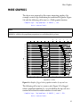
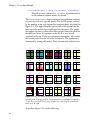
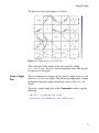
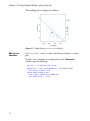
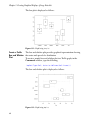
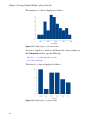
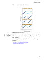
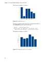
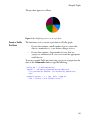
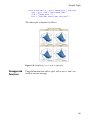
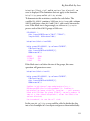
The clusterMeansCounts object contains mean population estimates
for each zip code area, age and gender. The first 24 groups (ordered
by the number of zip code regions that comprise them) are plotted in
Figure 2.11. The upper left panel corresponds to the group with the
most zip codes and the lower right panel has the fewest. The graphs
that appear top-heavy reflect more older people. Notice the panel in
the third row down, first position on the left. It is very heavily
weighted on the top. These are retirement communities. Also, notice
the second panel from the left in the bottom row. The population is
dominated by young adult males. These are primarily military bases.
k=2
N = 5533
k=4
N = 4807
k=3
N = 4235
k=6
N = 3204
k=5
N = 2839
k=7
N = 1711
k = 10
N = 1569
k=9
N = 1394
k=8
N = 1277
k = 11
N = 1260
k = 14
N = 1107
k = 12
N = 510
k = 13
N = 480
k = 17
N = 414
k = 16
N = 331
k = 15
N = 321
k = 21
N = 183
k = 23
N = 121
k = 22
N = 110
k = 18
N = 67
k = 19
N = 64
k = 20
N = 60
k = 26
N = 59
k = 25
N = 57
Figure 2.11: Age distribution barplots for the first 24 groups resulting from k-means
clustering with 40 groups specified. The horizontal lines in each panel correspond to
20 (the lower one) and 70 years of age. Females are to the left of the vertical and
males are to the right.
To produce Figure 2.11, run the following:
48
Clustering
> source(paste(getenv("SHOME"),
"/samples/bigdata/census/my.vbar.q", sep=""))
> index16 <- rep(1:16, length = 24)
> par(mfrow=c(4,6))
> for(k in 1:24) {
my.vbar(bd.coerce(clusterMeansCounts), k=k,
plotcols=3:38,
Nreport.col=2,
col=1+index16[k])
}
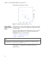
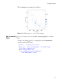
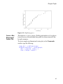
An interesting graphic that dramatizes group membership displays
each zip code as a single black point for the center of the zip code
region, and then overlays points for any given cluster group in
another color. Technically, this plot is more interesting, because it
uses a new function, bd.block.apply, to process the data a block at a
time.
The bd.block.apply function takes two primary arguments:
•
The data, usually a bdFrame, census in this case.
•
a function for processing the data a block at a time.
Note
The bd.block.apply argument FUN is an S-PLUS function called to process a data frame. This
function itself cannot perform big data operations, or an error is generated. (This is true for
bd.by.group and bd.by.window, as well.)
Define the block processing function as follows:
f <- function(SP){
par(plt = c(.1, 1, .1, 1))
if(SP$in1.pos == 1){
plot(SP$in1[,"long"], SP$in1[, "lat"],
pch = 1, cex = 0.15,
xlim=c(-125,-70), ylim=c(25, 50),
xlab="", ylab="", axes = F)
axis(1, cex = 0.5)
axis(2, cex = 0.5)
title(xlab = "Longitude", ylab = "Latitude")
} else {
49
Chapter 2 Census Data Example
points(SP$in1[, "long"], SP$in1[, "lat"], cex =
0.2)
}
}
This function processes a list object, which contains one block of the
census bdFrame. SP$in1 corresponds to the data, and SP$in1.pos
corresponds to the starting row position of each block of the bdFrame
that is passed to the function. The test if(SP$in1.pos == 1) checks if
the first block is being processed. If the first block is processed, a call
to plot is made; if the first block is not processed, a call to points is
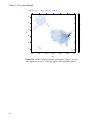
made. The call to bd.block.apply is:
> bd.block.apply(census, FUN = f)
This call makes this new graph select only those rows that belong to
the cluster group of interest, and then coerce it to a data frame to
demonstrate the simplicity of using both bdFrame and a data.frame
objects in the same function. Start by keeping only those variables
that are useful for displaying the cluster group locations.
> censusNPsub <- bd.filter.columns(censusNPred,
keep = c("lat","long","PREDICT.membership"))
50
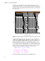
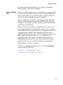
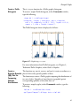
Clustering
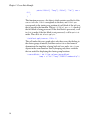
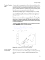
Figure 2.12: Plot of all zip code region centers with cluster group 20 overlaid in
another color. The double histogram in the bottom left corner displays the age
distributions for females to the left and males to the right for cluster group 20. The
horizontal lines in the histogram are at 20 and 70 years of age.
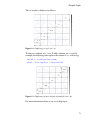
To generate graphs for the first 22 cluster groups, it is slightly more
work:
> pred <- clusterMeansCounts[, "PREDICT.membership"]
> for(k in 1:22) {
> setk <- bd.coerce(bd.filter.rows(censusNPsub,
expr = "PREDICT.membership == pred[k]",
columns = c("lat", "long"),
row.language = F))
par(plt=c(.1, 1, .1, 1))
bd.block.apply(census, FUN = f)
points(setk[, "long"], setk[, "lat"],
col=1+index16[k],
cex=0.6, pch=16)
par(new=T)
51
Chapter 2 Census Data Example
par(plt=c(.1, .3, .1, .3))
my.vbar(clusterMeansCounts, k=k, plotcols=3:38,
Nreport.col=2, col=1+index16[k])
box()
}
Notes
52
1.
is created as a regular data frame using bd.coerce, assuming that once a
given cluster group is selected the data is small enough to process it entirely in
memory.
2.
bd.block.apply
3.
setk contains the latitude and longitude locations for zip code centers for the
selected group, pred[k]
4.
setk was created to demonstrate the use of both bdFrame objects and data.frame
objects in a single function. Placing the cluster group points on the graph could
also be accomplished in the function passed to bd.block.apply.
setk
is used to plot all the zip code region centers, which requires
processing the entire bdFrame.
Modeling Group Membership
MODELING GROUP MEMBERSHIP
The age distributions in Figure 2.11 are intriguing, but we know little
about why the ages are distributed the way they are. Except for
obvious deductions like retirement communities and military bases,
we do not have much more information in the current data set.
Another data set, censusDemogr, provides additional demographics
variables such as household income, education and marital status.
By modeling group membership as a function of an assortment of
explanatory variables, we can characterize the groups relative to
those variables. The data in censusDemogr contains the variables
listed in Table 2.4. Note that all the variables except housingTotal
and the cluster group variables at the end contain the proportion of
households (hh) with the characteristic stated in the description
column.
Table 2.4: Variables contained in censusDemogr, a bdFrame object. All variables,
except housingTotal, contain the proportion of households (hh) in the zip code area
with the stated characteristic.
Variable
Description
housingTotal
Total number of housing units.
own
Own residence.
onePlusPersonHouse
Two or more family members in hh.
nonFamily
Two or more non-family members in hh.
Plus65InHouse
65 or older in family hh.
Plus65InNonFamily
65 or older in non-family hh.
Plus65InGroup
65 or older in group quarters.
marriedChildren
Married-couple families with children.
marriedNoChildren
Married-couple families without children.
53
Chapter 2 Census Data Example
Table 2.4: Variables contained in censusDemogr, a bdFrame object. All variables,
except housingTotal, contain the proportion of households (hh) in the zip code area
with the stated characteristic.
54
Variable
Description
maleChildren
Male householder with children.
maleNoChildren
Male householder without children.
femaleChildren
Female householder with children.
femaleNoChildren
Female householder without children.
maleSingle
Single male.
femaleSingle
Single female.
maleMarried
Married male.
femaleMarried
Married female.
maleWidow
Male widower.
femaleWidow
Female widow.
maleDiv
Male divorced.
femaleDiv
Female divorced.
english5to17
5 - 17 year olds speak only English.
english18to65
18 - 65 year olds speak only English.
englishOver65
Over 65 year olds speak only English.
native
Born in US.
entryToUS95to00
Entry to US from 1995 to 2000.
Modeling Group Membership
Table 2.4: Variables contained in censusDemogr, a bdFrame object. All variables,
except housingTotal, contain the proportion of households (hh) in the zip code area
with the stated characteristic.
Variable
Description
entryToUS90to94
Entry to US from 1990 to 1994.
entryToUS85to89
Entry to US from 1985 to 1989.
entryToUS80to84
Entry to US from 1980 to 1984.
entryToUS75to79
Entry to US from 1975 to 1979.
entryToUS70to74
Entry to US from 1970 to 1974.
entryToUS65to69
Entry to US from 1965 to 1969.
entryToUSBefore65
Entry to US before 1965.
changedHouseSince95
Changed residence since 1995.
maleLoEd
Male head of household with low education.
femaleLoEd
Female head of hh with low education.
maleHS
Male head of hh with HS education.
femaleHS
Female head of hh with HS education.
maleCollege
Male head of hh with college education.
femaleCollege
Female head of hh with college education.
maleBA
Male head of hh with bachelor’s degree.
femaleBA
Female head of hh with bachelor’s degree.
maleAdvDeg
Male head of hh with advanced degree.
55
Chapter 2 Census Data Example
Table 2.4: Variables contained in censusDemogr, a bdFrame object. All variables,
except housingTotal, contain the proportion of households (hh) in the zip code area
with the stated characteristic.
56
Variable
Description
femaleAdvDeg
Female head of hh with advanced degree.
maleWorked99
Male head of hh worked in 1999.
femaleWorked99
Female head of hh worked in 1999.
maleBlueCollar
Male head of hh blue-collar worker.
femaleBlueCollar
Female head of hh blue-collar worker.
maleWhiteCollar
Male head of hh white-collar worker.
femaleWhiteCollar
Female head of hh white-collar worker.
houseUnder30K
hh income under $30K.
house30to60K
hh income $30K - $60K.
house60to200K
hh income $60K - $200K.
houseOver200K
hh income over $200K.
houseWithSalary
hh with salary income.
houseSelfEmpl
hh with self-employment income.
houseInterestEtc
hh with interest and other investment income.
houseSS
hh with social security income.
housePubAssist
hh with public assistance income.
houseRetired
Head of hh retired.
Modeling Group Membership
Table 2.4: Variables contained in censusDemogr, a bdFrame object. All variables,
except housingTotal, contain the proportion of households (hh) in the zip code area
with the stated characteristic.
Building a
Model
Variable
Description
houseNotVacant
House not vacant.
houseOwnerOccupied
House owner occupied.
group18
Cluster group18.
The cluster group membership variables are binary with “yes” or
“no”, indicating group membership for each zip code area. To get a
sense of group membership characteristics, you can create a logistic
model for each group of interest using glm, which has been extended
to handle bdFrame objects. The syntax is identical to that of glm with
regular data frames.The model specification is as follows:
> group18Fit <- glm(group18 ~ ., data = censusDemogr,
family = binomial)
And the output is similar:
> group18Fit
Call:
bdGlm(formula = group18 ~ ., family = binomial, data
= censusDemogr)
Coefficients:
(Intercept) housingTotal
own
-51.49204 0.0002713171 -0.0005471851
onePlusPersonHouse nonFamily Plus65InHouse
3.560468 10.21905
18.44271
.
.
.
Degrees of freedom: 31951 total; 31888 residual
57
Chapter 2 Census Data Example
Residual Deviance: 5445.941
Note
The glm function call is the same as for regular in-memory data frames; however, the extended
version of glm in the bigdata library applies appropriate methods to bdFrame data by initiating a
call to bdGlm. The call expression shows the actual call went to bdGlm.
Summarizing
the Fit
You can apply the usual operations (for example, summary, coef,
plot) to the resulting fit object. The plots are displayed as hexbin
scatterplots because of the volume of data.
4
> plot(group18Fit)
Counts
-2
0
Residuals
2
31780
30000
28000
26000
24000
22000
20000
18000
16000
14000
12000
10000
8000
6000
4000
2000
1
0.0
0.2
0.4
0.6
0.8
1.0
Fitted : housingTotal + own + onePlusPersonHouse + nonFamily + Plus65InHouse + P .
Figure 2.13: Residuals vs. fitted values resulting from modeling cluster group 18
membership as a function of census demographics.
Characterizing
the Group
To characterize the group, examine the significant coefficients as
follows:
> group18Coeff <- summary(group18Fit)[["coef"]]
58
Modeling Group Membership
> group18Coeff[abs(group18Coeff[,"t value"])
> qnorm(0.975),]
Value Std. Error
t value
(Intercept) -51.492043 13.866083 -3.713525
nonFamily 10.219051
4.079199 2.505161
Plus65InHouse 18.442709
6.172655 2.987808
Plus65InNonFamily 19.186751
5.953835 3.222587
maleSingle 39.541568
9.123876 4.333857
femaleWidow 23.710092 10.332282 2.294759
maleDiv 23.374178
8.807237 2.653974
changedHouseSince95
6.253725
2.492780 2.508735
femaleLoEd -12.132175
2.986016 -4.062997
maleCollege
5.820187
2.897105 2.008966
femaleBA -9.518559
3.518594 -2.705217
maleAdvDeg 10.536835
3.553861 2.964898
femaleAdvDeg -7.932499
3.568260 -2.223072
maleWorked99
6.598822
2.787717 2.367107
femaleWorked99
7.200051
3.244321 2.219278
To interpret the above table, note that positive coefficients predict
group 18 membership and negative coefficients predict non-group
membership. With that understanding, group 18 members are more
likely:
•
In non-family households that have changed location in the
last 5 years.
•
Single or divorced males or widowed females.
•
Males with some college education and frequently with
advanced degrees who worked the previous year.
Cluster group 18 corresponds to zip code regions dominated by
young adult males, typical of military bases and penal institutions.
59
Chapter 2 Census Data Example
60
CREATING GRAPHICAL
DISPLAYS OF LARGE DATA
SETS
3
Introduction
62
Overview of Graph Functions
Functions Supporting Graphs
63
63
Example Graphs
Plotting Using Hexagonal Binning
Adding Reference Lines
Plotting by Summarizing Data
Creating Graphs with Preprocessing Functions
Unsupported Functions
69
69
74
79
90
103
61
Chapter 3 Creating Graphical Displays of Large Data Sets
INTRODUCTION
This chapter includes information on the following:
•
An overview of the graph functions available in the Big Data
Library, listed according to whether they take a big data
object directly, or require a preprocessing function to produce
a chart.
•
Procedures for creating plots, traditional graphs, and Trellis
graphs.
Note
In Microsoft Windows, editable graphs in the graphical user interface (GUI) do not support big
data objects. To use these graphs, create an S-Plus data.frame containing either all of the data or
a sample of the data.
62
Overview of Graph Functions
OVERVIEW OF GRAPH FUNCTIONS
The Big Data Library supports most (but not all) of the traditional and
Trellis graph functions available in the S-PLUS library. The design of
graph support for big data can be attributed to practical application.
For example, if you had a data set of a million rows or tens of
thousands of columns, a cloud chart would produce an illegible plot.
Functions
Supporting
Graphs
This section lists the functions that produce graphs for big data
objects. If you are unfamiliar with plotting and graph functions in
S-PLUS, review the Guide to Graphics.
Implementing plotting and graph functions to support large data sets
requires an intelligent way to handle thousands of data points. To
address this need, the graph functions to support big data are
designed in the following categories:
•
Functions to plot big data objects without preprocessing,
including:
•
Functions to plot big data objects by hexagonal binning.
•
Functions to plot big data objects by summarizing data in
a plot-specific manner.
•
Functions providing the preprocessing support for plotting big
data objects.
•
Functions requiring preprocessing support to plot big data
objects.
The following sections list the functions, organized into these
categories. For an alphabetical list of graph functions supporting big
data objects, see the Appendix.
Using cloud or parallel results in an error message. Instead, sample
or aggregate the data to create a data.frame that can be plotted using
these functions.
63
Chapter 3 Creating Graphical Displays of Large Data Sets
Graph Functions
using Hexagonal
Binning
The following functions can plot a large data set (that is, can accept a
big data object without preprocessing) by plotting large amounts of
data using hexagonal binning.
Table 3.1: Functions for plotting big data using hexagonal binning.
Function
Comment
pairs
Can accept a bdFrame object.
plot
Can accept a hexbin, a single bdVector, two bdVectors,
or a bdFrame object.
splom
Creates a Trellis graphic object of a scatterplot matrix.
xyplot
Creates a Trellis graphic object, which graphs one set
of numerical values on a vertical scale against another
set of numerical values on a horizontal scale.
Functions Adding Reference Lines to Plots
The following functions add reference lines to hexbin plots.
Table 3.2: Functions that add reference lines to hexbin plots.
64
Function
Type of line
abline(lsfit())
Regression line.
lines(loess.smooth())
Loess smoother.
lines(smooth.spline())
Smoothing spline.
panel.lmline
Adds a least squares line to an
xyplot in a Trellis graph.
Overview of Graph Functions
Table 3.2: Functions that add reference lines to hexbin plots. (Continued)
Graph Functions
Summarizing
Data
Function
Type of line
panel.loess
Adds a loess smoother to an xyplot
in a Trellis graph.
qqline()
QQ-plot reference line.
xyplot(lmline=T)
Adds a least squares line to an
xyplot in a Trellis graph.
The following functions summarize data in a plot-specific manner to
plot big data objects.
Table 3.3: Functions that summarize in plot-specific manner.
Function
Description
boxplot
Produces side by side boxplots from a number of
vectors. The boxplots can be made to display the
variability of the median, and can have variable widths
to represent differences in sample size.
bwplot
Produces a box and whisker Trellis graph, which you
can use to compare the distributions of several data
sets.
plot(density)
density returns x and y coordinates of a nonparametric estimate of the probability density of the
data.
densityplot
Produces a Trellis graph demonstrating the
distribution of a single set of data.
hist
Creates a histogram.
histogram
Creates a histogram in a Trellis graph.
qq
Creates a Trellis graphic object comparing the
distributions of two sets of data
65
Chapter 3 Creating Graphical Displays of Large Data Sets
Table 3.3: Functions that summarize in plot-specific manner. (Continued)
Functions
Providing
Support to
Preprocess Data
for Graphing
66
Function
Description
qqmath
Creates normal probability plot for only one data
object in a Trellis graph. qqmath can also make
probability plots for other distributions. It has an
argument distribution whose input is any function that
computes quantiles.
qqnorm
Creates normal probability plot in a Trellis graph.
qqnorm can accept a single bdVector object.
qqplot
Creates normal probability plot in a Trellis graph. Can
accept two bdVector objects. In qqplot, each vector or
bdVector is taken as a sample, for the x- and y-axis
values of an empirical probability plot.
stripplot
Creates a Trellis graphic object similar to a box plot in
layout; however, it displays the density of the
datapoints as shaded boxes.
The following functions are used to preprocess large data sets for
graphing:
Table 3.4: Functions used for preprocessing large data sets.
Function
Description
aggregate
Splits up data by time period or other factors
and computes summary for each subset.
hexbin
Creates an object of class hexbin. Its basic
components are a cell identifier and a count of
the points falling into each occupied cell.
hist2d
Returns a structure for a 2-dimensional
histogram which can be given to a graphics
function such as image or persp.
interp
Interpolates the value of the third variable onto
an evenly spaced grid of the first two variables.
Overview of Graph Functions
Table 3.4: Functions used for preprocessing large data sets. (Continued)
Functions
Requiring
Preprocessing
Support for
Graphing
Function
Description
loess
Fits a local regression model.
loess.smooth
Returns a list of values at which the loess curve
is evaluated.
lsfit
Fits a (weighted) least squares multivariate
regression.
smooth.spline
Fits a cubic B-spline smooth to the input data.
table
Returns a contingency table (array) with the
same number of dimensions as arguments
given.
tapply
Partitions a vector according to one or more
categorical indices.
The following functions do not accept a big data object directly to
create a graph; rather, they require one of the specified preprocessing
functions.
Table 3.5: Functions requiring preprocessors for graphing
large data sets.
Function
Preprocessors
Description
barchart
table, tapply,
aggregate
Creates a bar chart in a Trellis
graph.
barplot
table, tapply,
aggregate
Creates a bar graph.
contour
interp, hist2d
Make a contour plot and possibly
return coordinates of contour lines.
contourplot
loess
Displays contour plots and level
plots in a Trellis graph.
67
Chapter 3 Creating Graphical Displays of Large Data Sets
Table 3.5: Functions requiring preprocessors for graphing
large data sets. (Continued)
68
Function
Preprocessors
Description
dotchart
table, tapply,
aggregate
Plots a dot chart from a vector.
dotplot
table, tapply,
aggregate
Creates a Trellis graph, displaying
dots and labels.
image
interp, hist2d
Creates an image, under some
graphics devices, of shades of gray
or colors that represent a third
dimension.
levelplot
loess
Displays a level plot in a Trellis
graph.
persp
interp, hist2d
Creates a perspective plot, given a
matrix that represents heights on an
evenly spaced grid.
pie
table, tapply,
aggregate
Creates a pie chart from a vector of
data.
piechart
table, tapply,
aggregate
Creates a pie chart in a Trellis graph
wireframe
loess
Displays a three-dimensional
wireframe plot in a Trellis graph.
Example Graphs
EXAMPLE GRAPHS
The examples in this chapter require that you have the Big Data
Library loaded. The examples are not large data sets; rather, they are
small data objects that you convert to big data objects to demonstrate
using the Big Data Library graphing functions.
Plotting Using
Hexagonal
Binning
Hexagonal binning plots are available for:
•
Single plot (plot)
•
Matrix of plots (pairs)
•
Conditioned single or matrix plots (xyplot)
Functions that evaluate data over a grid in standard S-PLUS aggregate
the data over the grid (such as binning the data and taking the mean
in each grid cell, and then plot the aggregated values) when applied to
a big data object.
Hexagonal binning is a data grouping or reduction method typically
used on large data sets to clarify a spatial display structure in two
dimensions. Think of it as partitioning a scatter plot into larger units
to reduce dimensionality, while maintaining a measure of data clarity.
Each unit of data is displayed with a hexagon and represents a bin of
points in the plot. Hexagons are used instead of squares or rectangles
to avoid misleading structure that occurs when edges of the rectangles
line up exactly.
Plotting using hexagonal binning is the standard technique used when
a plotting function that currently plots one point per row is applied to
a big data object.
Plotting using hexagonal bins is available for a single plot, a matrix of
plots, and conditioned single or matrix plots.
69
Chapter 3 Creating Graphical Displays of Large Data Sets
The Census example introduced in Chapter 2 demonstrates plotting
using hexagonal binning (see Figure 2.6). When you create a plot
showing a distribution of zip codes by latitude and longitude, the
following simple plot is displayed:
Figure 3.1: Example of graph showing hexagonal binning.
The functions listed in Table 3.1 support big data objects by using
hexagonal binning. This section shows examples of how to call these
functions for a big data object.
Create a PairThe pairs function creates a figure that contains a scatter plot for
wise Scatter Plot each pair of variables in a bdFrame object.
To create a sample pair-wise scatter plot for the fuel.frame bdFrame
object, in the Commands window, type the following:
pairs(as.bdFrame(fuel.frame))
70
Example Graphs
The pair-wise scatter plot appears as follows:
fif
Figure 3.2: Graph using pairs for a bdFrame.
This scatter plot looks similar to the one created by calling
pairs(fuel.frame); however, close examination shows that the plot
is composed of hexagons.
Create a Single
Plot
The plot function can accept a hexbin object, a single bdVector, two
bdVectors, or a bdFrame object. The following example plots a simple
hexbin plot using the weight and mileage vectors of the fuel.bd
object.
To create a sample single plot, in the Commands window, type the
following:
fuel.bd <- as.bdFrame(fuel.frame)
plot(hexbin(fuel.bd$Weight, fuel.bd$Mileage))
71
Chapter 3 Creating Graphical Displays of Large Data Sets
The hexbin plot is displayed as follows:
Figure 3.3: Graph using single hexbin plot for fuel.bd.
Create a MultiThe function splom creates a Trellis graph of a scatterplot matrix. The
Panel Scatterplot scatterplot matrix is a good tool for displaying measurements of three
or more variables.
Matrix
To create a sample multi-panel scatterplot matrix, where you create a
hexbin plot of the columns in fuel.bd against each other, in the
Commands window, type the following:
fuel.bd <- as.bdFrame(fuel.frame)
splom(~., data=fuel.bd)
Note
Trellis functions in the Big Data Library require the data argument. You cannot use formulas
that refer to bdVectors that are not in a specified bdFrame.
Notice that the ‘.’ is interpreted as all columns in the data set
specified by data.
72
Example Graphs
The splom plot is displayed as follows:
Figure 3.4: Graph using splom for fuel.bd.
To remove a column, use -term. To add a column, use +term. For
example, the following code replaces the column Disp. with its log.
fuel.bd <- as.bdFrame(fuel.frame)
splom(~.-Disp.+log(Disp.), data=fuel.bd)
Figure 3.5: Graph using splom to designate a formula for fuel.bd
For more information about splom, see its help topic.
73
Chapter 3 Creating Graphical Displays of Large Data Sets
Create a
The function xyplot creates a Trellis graph, which graphs one set of
Conditioning Plot numerical values on a vertical scale against another set of numerical
values on a horizontal scale.
or Scatter Plot
To create a sample conditioning plot, in the Commands window,
type the following:
xyplot(data=as.bdFrame(air),
ozone~radiation|temperature,
shingle.args=list(n=4), lmline=T)
The variable on the left of the ~ goes on the vertical (or y) axis, and
the variable on the right goes on the horizontal (or x) axis.
The function xyplot contains the default argument lmline=T to add
the approximate least squares line to a panel quickly. This argument
performs the same action as panel.lmline in standard S-PLUS.
The xyplot plot is displayed as follows:
Figure 3.6: Graph using xyplot with lmline=T.
Trellis functions in the Big Data Library handle continuous “given”
variables differently than standard data Trellis functions: they are sent
through equal.count, rather than factor.
Adding
Reference
Lines
74
You can add a regression line or scatterplot smoother to hexbin plots.
The regression line or smoother is a weighted fit, based on the binned
values.
Example Graphs
The following functions add the following types of reference lines to
hexbin plots:
•
A regression line with abline
•
A Loess smoother with loess.smooth
•
A smooth spline with smooth.spline
•
A line to a qqplot with qqline
•
A least squares line to an xyplot in a Trellis graph.
For smooth.spline and loess.smooth, when the data consists of
bdVectors, the data is aggregated before smoothing. The range of the
x variable is divided into 1000 bins, and then the mean for x and y is
computed in each bin. A weighted smooth is then computed on the
bin means, weighted based on the bin counts. This computation
results in values that differ somewhat from those where the smoother
is applied to the unaggregated data. The values are usually close
enough to be indistinguishable when used in a plot, but the difference
could be important when the smoother is used for prediction or
optimization.
Add a Regression When you create a scatterplot from your large data set, and you
notice a linear association between the y-axis variable and the x-axis
Line
variable, you might want to display a straight line that has been fit to
the data. Call lsfit to perform a least squares regression, and then
use that regression to plot a regression line.
The following example draws an abline on the chart that plots
fuel.bd weight and mileage data. First, create a hexbin object and
plot it, and then add the abline to the plot.
To add a regression line to a sample plot, in the Commands window,
type the following:
fuel.bd <- as.bdFrame(fuel.frame)
hexbin.out <- plot(fuel.bd$Weight, fuel.bd$Mileage)
# displays a hexbin plot
# use add.to.hexbin to keep the abline within the
# hexbin area. If you just call abline, then the
# line might draw outside of the hexbin and interfere
# with the label.
add.to.hexbin(hexbin.out, abline(lsfit(fuel.bd$Weight,
fuel.bd$Mileage)))
75
Chapter 3 Creating Graphical Displays of Large Data Sets
The resulting chart is displayed as follows:
Figure 3.7: Graph drawing an abline in a hexbin plot.
Add a Loess
Smoother
Use lines(loess.smooth) to add a smooth curved line to a scatter
plot.
To add a loess smoother to a sample plot, in the Commands
window, type the following:
fuel.bd <- as.bdFrame(fuel.frame)
hexbin.out <- plot(fuel.bd$Weight, fuel.bd$Mileage)
# displays a hexbin plot
add.to.hexbin(hexbin.out,
lines(loess.smooth(fuel.bd$Weight,
fuel.bd$Mileage), lty=2))
76
Example Graphs
The resulting chart is displayed as follows:
Figure 3.8: Graph using loess.smooth in a hexbin plot.
Add a Smoothing Use lines(smooth.spline) to add a smoothing spline to a scatter
plot.
Spline
To add a smoothing spline to a sample plot, in the Commands
window, type the following:
fuel.bd <- as.bdFrame(fuel.frame)
hexbin.out <- plot(fuel.bd$Weight, fuel.bd$Mileage)
# displays a hexbin plot
add.to.hexbin(hexbin.out,
lines(smooth.spline(fuel.bd$Weight,
fuel.bd$Mileage),lty=3))
77
Chapter 3 Creating Graphical Displays of Large Data Sets
The resulting chart is displayed as follows:
Figure 3.9: Graph using smooth.spline in a hexbin plot.
Add a Least
Squares Line to
an xyplot
To add a reference line to an xyplot, set lmline=T. Alternatively, you
can call panel.lmline or panel.loess. See the section Create a
Conditioning Plot or Scatter Plot on page 74 for an example.
Add a qqplot
Reference Line
The function qqline fits and plots a line through a normal qqplot.
To add a qqline reference line to a sample qqplot, in the
Commands window, type the following:
fuel.bd <- as.bdFrame(fuel.frame)
qqnorm(fuel.bd$Mileage)
qqline(fuel.bd$Mileage)
78
Example Graphs
The qqline chart is displayed as follows:
Figure 3.10: Graph using qqline in a qqplot chart.
Plotting by
Summarizing
Data
The following examples demonstrate functions that summarize data
in a plot-specific manner to plot big data objects. These functions do
not use hexagonal binning. Because the plots for these functions are
always monotonically increasing, hexagonal binning would obscure
the results. Rather, summarizing provides the appropriate
information.
Create a Box Plot The following example creates a simple box plot from fuel.bd. To
create a Trellis box and whisker plot, see the following section.
To create a sample box plot, in the Commands window, type the
following:
fuel.bd <- as.bdFrame(fuel.frame)
boxplot(split(fuel.bd$Fuel, fuel.bd$Type), style.bxp="att")
79
Chapter 3 Creating Graphical Displays of Large Data Sets
The box plot is displayed as follows:
Figure 3.11: Graph using boxplot.
Create a Trellis
The box and whisker plot provides graphical representation showing
Box and Whisker the center and spread of a distribution.
Plot
To create a sample box and whisker plot in a Trellis graph, in the
Commands window, type the following:
bwplot(Type~Fuel, data=(as.bdFrame(fuel.frame)))
The box and whisker plot is displayed as follows:
Figure 3.12: Graph using bwplot.
80
Example Graphs
For more information about bwplot, see Chapter 3, Traditional
Trellis Graphics, in the Guide to Graphics.
Create a Density
Plot
The density function returns x and y coordinates of a non-parametric
estimate of the probability density of the data. Options include the
choice of the window to use and the number of points at which to
estimate the density. Weights may also be supplied.
Density estimation is essentially a smoothing operation. Inevitably
there is a trade-off between bias in the estimate and the estimate's
variability: wide windows produce smooth estimates that may hide
local features of the density.
Density summarizes data. That is, when the data is a bdVector, the
data is aggregated before smoothing. The range of the x variable is
divided into 1000 bins, and the mean for x is computed in each bin. A
weighted density estimate is then computed on the bin means,
weighted based on the bin counts. This calculation gives values that
differ somewhat from those when density is applied to the
unaggregated data. The values are usually close enough to be
indistinguishable when used in a plot, but the difference could be
important when density is used for prediction or optimization.
To plot density, use the plot function.
To create a sample density plot from fuel.bd, in the Commands
window, type the following:
fuel.bd <- as.bdFrame(fuel.frame)
plot(density(fuel.bd$Weight), type="l")
81
Chapter 3 Creating Graphical Displays of Large Data Sets
The density plot is displayed as follows:
Figure 3.13: Graph using density
Create a Trellis
Density Plot
The following example creates a Trellis graph of a density plot, which
displays the shape of a distribution. You can use the Trellis density
plot for analyzing a one-dimensional data distribution. A density plot
displays an estimate of the underlying probability density function for
a data set, allowing you to approximate the probability that your data
fall in any interval.
To create a sample Trellis density plot, in the Commands window,
type the following:
singer.bd <- as.bdFrame(singer)
densityplot( ~ height | voice.part, data = singer.bd,
layout = c(2, 4), aspect= 1, xlab = "Height (inches)",
width = 5)
82
Example Graphs
The Trellis density plot is displayed as follows:
Figure 3.14: Graph using densityplot.
For more information about Trellis density plots, see Chapter 3,
Traditional Trellis Graphics, in the Guide to Graphics.
Create a Simple
Histogram
A histogram displays the number of data points that fall in each of a
specified number of intervals. A histogram gives an indication of the
relative density of the data points along the horizontal axis. For this
reason, density plots are often superposed with (scaled) histograms.
To create a sample hist chart of a full dataset for a numeric vector, in
the Commands window, type the following:
fuel.bd <- as.bdFrame(fuel.frame)
hist(fuel.bd$Weight)
83
Chapter 3 Creating Graphical Displays of Large Data Sets
The numeric hist chart is displayed as follows:
Figure 3.15: Graph using hist for numeric data.
To create a sample hist chart of a full dataset for a factor column, in
the Commands window, type the following:
fuel.bd <- as.bdFrame(fuel.frame)
hist(fuel.bd$Type)
The factor hist chart is displayed as follows:
Figure 3.16: Graph using hist for factor data.
84
Example Graphs
Create a Trellis
Histogram
The histogram function for a Trellis graph is histogram.
To create a sample Trellis histogram, in the Commands window,
type the following:
singer.bd <- as.bdFrame(singer)
histogram( ~ height | voice.part, data = singer.bd,
nint = 17, endpoints = c(59.5, 76.5), layout = c(2,4),
aspect = 1, xlab = "Height (inches)")
The Trellis histogram chart is displayed as follows:
Figure 3.17: Graph using histogram.
For more information about Trellis histograms, see Chapter 3,
Traditional Trellis Graphics, in the Guide to Graphics.
Create a
Quantile-Quantile
(QQ) Plot for
Comparing
Multiple
Distributions
The functions qq, qqmath, qqnorm, and qqplot create an ordinary x-y
plot of 500 evenly-spaced quantiles of data.
The function qq creates a Trellis graph comparing the distributions of
two sets of data. Quantiles of one dataset are graphed against
corresponding quantiles of the other data set.
To create a sample qq plot, in the Commands window, type the
following:
fuel.bd <- as.bdFrame(fuel.frame)
qq((Type=="Compact")~Mileage, data = fuel.bd)
85
Chapter 3 Creating Graphical Displays of Large Data Sets
The factor on the left side of the ~ must have exactly two levels
(fuel.bd$Compact has five levels).
The qq plot is displayed as follows:
f
Figure 3.18: Graph using qq.
(Note that in this example, by setting Type to the logical Compact, the
labels are set to FALSE and TRUE on the x and y axis, respectively.)
Create a QQ Plot
Using a
Theoretical or
Empirical
Distribution
The function qqmath creates normal probability plot in a Trellis
graph. that is, the ordered data are graphed against quantiles of the
standard normal distribution.
can also make probability plots for other distributions. It has
an argument distribution, whose input is any function that
computes quantiles. The default for distribution is qnorm. If you set
distribution = qexp, the result is an exponential probability plot.
qqmath
To create a sample qqmath plot, in the Commands window, type the
following:
singer.bd <- as.bdFrame(singer)
qqmath( ~ height | voice.part, data = singer.bd,
layout = c(2, 4), aspect = 1,
xlab = "Unit Normal Quantile",
ylab = "Height (inches)")
86
Example Graphs
The qqmath plot is displayed as follows:
Figure 3.19: Graph using qqmath.
Create a Single
Vector QQ Plot
The function qqnorm creates a plot using a single bdVector object. The
following example creates a plot from the mileage vector of the
fuel.bd object.
To create a sample qqnorm plot, in the Commands window, type the
following:
fuel.bd <- as.bdFrame(fuel.frame)
qqnorm(fuel.bd$Mileage)
87
Chapter 3 Creating Graphical Displays of Large Data Sets
The qqnorm plot is displayed as follows:
Figure 3.20: Graph using qqnorm.
Create a Two
Vector QQ Plot
The function qqplot creates a hexbin plot using two bdVectors. The
quantile-quantile plot is a good tool for determining a good
approximation to a data set’s distribution. In a qqplot, the ordered
data are graphed against quantiles of a known theoretical distribution.
To create a sample two-vector qqplot, In the Commands window,
type the following:
fuel.bd <- as.bdFrame(fuel.frame)
qqplot(fuel.bd$Mileage, runif(length(fuel.bd$Mileage),
bigdata=T))
Note that in this example, the required y argument for qqplot is
runif(length(fuel.bd$Mileage): the random generation for the
uniform distribution for the vector fuel.bd$Mileage. Also note that
using runif with a big data object requires that you set the runif
argument bigdata=T.
The qqplot plot is displayed as follows:
88
Example Graphs
Figure 3.21: Graph using qqplot.
Create a OneDimensional
Scatter Plot
The function stripplot creates a Trellis graph similar to a box plot in
layout; however, the individual data points are shown instead of the
box plot summary.
To create sample one-dimensional scatter plot, in the Commands
window, type the following:
singer.bd <- as.bdFrame(singer)
stripplot(voice.part ~ jitter(height),
data = singer.bd, aspect = 1,
xlab = "Height (inches)")
89
Chapter 3 Creating Graphical Displays of Large Data Sets
The stripplot plot is displayed as follows:
Figure 3.22: Graph using stripplot for singer.bd.
Creating
Graphs with
Preprocessing
Functions
The functions discussed in this section do not accept a big data object
directly to create a graph; rather, they require a preprocessing
function such as those listed in the section Functions Providing
Support to Preprocess Data for Graphing on page 66.
Create a Bar
Chart
Calling barchart directly on a large data set produces a large number
of bars, which results in an illegible plot.
•
If your data contains a small number of cases, convert the
data to a standard data.frame before calling barchart.
•
If your data contains a large number of cases, first use
aggregate, and then use bd.coerce to create the appropriate
small data set.
In the following example, sum the yields over sites to get the total
yearly yield for each variety.
90
Example Graphs
To create a sample bar chart, in the Commands window, type the
following:
barley.bd <- as.bdFrame(barley)
temp.df <- bd.coerce(aggregate(barley.bd$yield,
list(year=barley.bd$year,
variety=barley.bd$variety), sum))
barchart(variety ~ x | year, data = temp.df,
aspect = 0.4,xlab = "Barley Yield (bushels/acre)")
The resulting bar chart appears as follows:
Figure 3.23: Graph using barchart .
Create a Bar Plot The following example creates a simple bar plot from fuel.bd, using
table
to preprocess data.
To create a sample bar plot using table to preprocess the data, in the
Commands window, type the following:
fuel.bd <- as.bdFrame(fuel.frame)
barplot(table(fuel.bd$Type), names=levels(fuel.bd$Type),
ylab="Count")
91
Chapter 3 Creating Graphical Displays of Large Data Sets
The bar plot is displayed as follows:
Figure 3.24: Graph using barplot.
To create a sample bar plot using tapply to preprocess the data, in
the Commands window, type the following:
fuel.bd <- as.bdFrame(fuel.frame)
barplot(tapply(fuel.bd$Mileage, fuel.bd$Type, mean),
names=levels(fuel.bd$Type), ylab="Average Mileage")
The bar plot is displayed as follows:
Figure 3.25: Graph using tapply to create a bar plot.
92
Example Graphs
Create a Contour A contour plot is a representation of three-dimensional data in a flat,
two-dimensional plane. Each contour line represents a height in the z
Plot
direction from the corresponding three-dimensional surface. A level
plot is essentially identical to a contour plot, but it has default options
that allow you to view a particular surface differently.
The following example creates a contour plot from fuel.bd, using
to preprocess data. For more information about interp, see
the section Visualizing Three-Dimensional Data in the Application
Developer’s Guide.
interp
Like density, interp and loess summarize the data. That is, when
the data is a bdVector, the data is aggregated before smoothing. The
range of the x variable is divided into 1000 bins, and the mean for x
computed in each bin. See the section Create a Density Plot on page
81 for more information.
To create a sample contour plot using interp to preprocess the data,
in the Commands window, type the following:
fuel.bd <- as.bdFrame(fuel.frame)
contour(interp(fuel.bd$Weight, fuel.bd$Disp.,
fuel.bd$Mileage))
The contour plot is displayed as follows:
Figure 3.26: Graph using interp to create a contour plot.
Create a Trellis
Contour Plot
The function contourplot creates a Trellis contour plot. The
contourplot function creates a Trellis graph of a contour plot. For big
data sets, contourplot requires a preprocessing function such as
loess.
93
Chapter 3 Creating Graphical Displays of Large Data Sets
The following example creates a contour plot of predictions from
loess.
To create a sample Trellis contour plot using loess to preprocess
data, in the Commands window, type the following:
environ.bd <- as.bdFrame(environmental)
{
ozo.m <- loess((ozone^(1/3)) ~
wind * temperature * radiation,data = environ.bd,
parametric = c("radiation", "wind"),
span = 1, degree = 2)
w.marginal <- seq(min(environ.bd$wind),
max(environ.bd$wind), length = 50)
t.marginal <- seq(min(environ.bd$temperature),
max(environ.bd$temperature), length = 50)
r.marginal <- seq(min(environ.bd$radiation),
max(environ.bd$radiation), length = 4)
wtr.marginal <- list(wind = w.marginal,
temperature = t.marginal, radiation = r.marginal)
grid <- expand.grid(wtr.marginal)
grid[, "fit"] <- c(predict(ozo.m, grid))
print(contourplot(fit ~ wind * temperature | radiation,
data = grid, xlab = "Wind Speed (mph)",
ylab = "Temperature (F)",
main = "Cube Root Ozone (cube root ppb)"))
}
94
Example Graphs
The Trellis contour plot is displayed as follows:
Figure 3.27: Graph using loess to create a Trellis contour plot.
Create a Dot
Chart
When you create a dot chart, you can use a grouping variable and
group summary, along with other options. The function dotchart can
be preprocessed using either table or tapply.
To create a sample dot chart using table to preprocess data, in the
Commands window, type the following:
fuel.bd <- as.bdFrame(fuel.frame)
dotchart(table(fuel.bd$Type), labels=levels(fuel.bd$Type),
xlab="Count")
95
Chapter 3 Creating Graphical Displays of Large Data Sets
The dot chart is displayed as follows:
Figure 3.28: Graph using table to create a dot chart.
To create a sample dot chart using tapply to preprocess data, in the
Commands window, type the following:
fuel.bd <- as.bdFrame(fuel.frame)
dotchart(tapply(fuel.bd$Mileage, fuel.bd$Type, median),
labels=levels(fuel.bd$Type), xlab="Median Mileage")
The dot chart is displayed as follows:
Figure 3.29: Graph using tapply to create a dot chart.
96
Example Graphs
Create a Dot Plot The function dotplot creates a Trellis graph that displays that
displays dots and gridlines to mark the data values in dot plots. The
dot plot reduces most data comparisons to straightforward length
comparisons on a common scale.
When using dotplot on a big data object, call dotplot after using
aggregate to reduce size of data.
In the following example, sum the barley yields over sites to get the
total yearly yield for each variety.
To create a sample dot plot, in the Commands window, type the
following:
barley.bd <- as.bdFrame(barley)
temp.df <- bd.coerce(aggregate(barley.bd$yield,
list(year=barley.bd$year, variety=barley.bd$variety),
sum))
(dotplot(variety ~ x | year, data = temp.df,
aspect = 0.4, xlab = "Barley Yield (bushels/acre)"))
The resulting Trellis dot plot appears as follows:
Figure 3.30: Graph using aggregate to create a dot chart.
Create an Image
Graph Using
hist2d
The following example creates an image graph using hist2d to
preprocess data. The function image creates an image, under some
graphics devices, of shades of gray or colors that represent a third
dimension.
97
Chapter 3 Creating Graphical Displays of Large Data Sets
To create a sample image plot using hist2d preprocess the data, in
the Commands window, type the following:
fuel.bd <- as.bdFrame(fuel.frame)
image(hist2d(fuel.bd$Weight, fuel.bd$Mileage, nx=9, ny=9))
The image plot is displayed as follows:
Figure 3.31: Graph using hist2d to create an image plot.
Create a Trellis
Level Plot
The levelplot function creates a Trellis graph of a level plot. For big
data sets, levelplot requires a preprocessing function such as loess.
A level plot is essentially identical to a contour plot, but it has default
options so you can view a particular surface differently. Like contour
plots, level plots are representations of three-dimensional data in flat,
two-dimensional planes. Instead of using contour lines to indicate
heights in the z direction, level plots use colors. The following
example produces a level plot of predictions from loess.
To create a sample Trellis level plot using loess to preprocess the
data, in the Commands window, type the following:
environ.bd <- as.bdFrame(environmental)
{
ozo.m <- loess((ozone^(1/3)) ~
wind * temperature * radiation, data = environ.bd,
parametric = c("radiation", "wind"),
span = 1, degree = 2)
98
Example Graphs
w.marginal <- seq(min(environ.bd$wind),
max(environ.bd$wind), length = 50)
t.marginal <- seq(min(environ.bd$temperature),
max(environ.bd$temperature), length = 50)
r.marginal <- seq(min(environ.bd$radiation),
max(environ.bd$radiation), length = 4)
wtr.marginal <- list(wind = w.marginal,
temperature = t.marginal, radiation = r.marginal)
grid <- expand.grid(wtr.marginal)
grid[, "fit"] <- c(predict(ozo.m, grid))
print(levelplot(fit ~ wind * temperature | radiation,
data = grid, xlab = "Wind Speed (mph)",
ylab = "Temperature (F)",
main = "Cube Root Ozone (cube root ppb)"))
}
The level plot is displayed as follows:
Figure 3.32: Graph using loess to create a level plot.
Create a persp
Graph Using
hist2d
The persp function creates a perspective plot given a matrix that
represents heights on an evenly spaced grid. For more information
about persp, see the section Perspective Plots in the Application
Developer’s Guide.
To create a sample persp graph using hist2d to preprocess the data,
in the Commands window, type the following:
fuel.bd <- as.bdFrame(fuel.frame)
persp(hist2d(fuel.bd$Weight, fuel.bd$Mileage))
99
Chapter 3 Creating Graphical Displays of Large Data Sets
The persp graph is displayed as follows:
Figure 3.33: Graph using hist2d to create a perspective plot
Hint
Using persp of interp might produce a more attractive graph.
Create a Pie
Chart
A pie chart shows the share of individual values in a variable, relative
to the sum total of all the values. Pie charts display the same
information as bar charts and dot plots, but can be more difficult to
interpret. This is because the size of a pie wedge is relative to a sum,
and does not directly reflect the magnitude of the data value. Because
of this, pie charts are most useful when the emphasis is on an
individual item’s relation to the whole; in these cases, the sizes of the
pie wedges are naturally interpreted as percentages.
Calling pie directly on a big data object can result in a pie with
thousands of wedges; therefore, preprocess the data using table to
reduce the number of wedges.
To create a sample pie chart using table to preprocess the data, in the
Commands window, type the following:
fuel.bd <- as.bdFrame(fuel.frame)
pie(table(fuel.bd$Type), names=levels(fuel.bd$Type),
sub="Count")
100
Example Graphs
The pie chart appears as follows:
fif
Figure 3.34: Graph using table to create a pie chart.
Create a Trellis
Pie Chart
The function piechart creates a pie chart in a Trellis graph.
•
If your data contains a small number of cases, convert the
data to a standard data.frame before calling piechart.
•
If your data contains a large number of cases, first use
aggregate, and then use bd.coerce to create the appropriate
small data set.
To create a sample Trellis pie chart using aggregate to preprocess the
data, in the Commands window, type the following:
barley.bd <- as.bdFrame(barley)
temp.df <- bd.coerce(aggregate(barley.bd$yield,
list(year=barley.bd$year, variety=barley.bd$variety),
sum))
piechart(variety ~ x | year, data = temp.df,
xlab = "Barley Yield (bushels/acre)")
101
Chapter 3 Creating Graphical Displays of Large Data Sets
The Trellis pie chart appears as follows:
Figure 3.35: Graph using aggregate to create a Trellis pie chart.
Create a Trellis
A surface plot is an approximation to the shape of a threeWireframe Plot dimensional data set. Surface plots are used to display data collected
on a regularly-spaced grid; if gridded data is not available,
interpolation is used to fit and plot the surface. The Trellis function
that displays surface plots is wireframe.
For big data sets, wireframe requires a preprocessing function such as
loess.
To create a sample Trellis surface plot using loess to preprocess the
data, in the Commands window, type the following:
environ.bd <- as.bdFrame(environmental)
{
ozo.m <- loess((ozone^(1/3)) ~
wind * temperature * radiation, data = environ.bd,
parametric = c("radiation", "wind"),
span = 1, degree = 2)
w.marginal <- seq(min(environ.bd$wind),
max(environ.bd$wind), length = 50)
t.marginal <- seq(min(environ.bd$temperature),
max(environ.bd$temperature), length = 50)
r.marginal <- seq(min(environ.bd$radiation),
max(environ.bd$radiation), length = 4)
wtr.marginal <- list(wind = w.marginal,
temperature = t.marginal, radiation = r.marginal)
grid <- expand.grid(wtr.marginal)
grid[, "fit"] <- c(predict(ozo.m, grid))
102
Example Graphs
print(wireframe(fit ~ wind * temperature | radiation,
data = grid, xlab = "Wind Speed (mph)",
ylab = "Temperature (F)",
main = "Cube Root Ozone (cube root ppb)"))
}
The surface plot is displayed as follows:
Figure 3.36: Graph using loess to create a surface plot.
Unsupported
Functions
Using the functions that add to a plot, such as points and lines,
results in an error message.
103
Chapter 3 Creating Graphical Displays of Large Data Sets
104
ADVANCED PROGRAMMING
INFORMATION
4
Introduction
106
Big Data Block Size Issues
Block Size Options
Group or Window Blocks
107
107
110
Big Data String and Factor Issues
String Column Widths
String Widths and importData
String Widths and bd.create.columns
Factor Column Levels
String Truncation and Level Overflow Errors
113
113
113
115
116
117
Storing and Retrieving Large S Objects
Managing Large Amounts of Data
119
119
Increasing Efficiency
bd.select.rows
bd.filter.rows
bd.create.columns
121
121
121
122
105
Chapter 4 Advanced Programming Information
INTRODUCTION
As an S-PLUS Big Data library user, you might encounter unexpected
or unusual behavior when you manipulate blocks of data or work
with strings and factors.
This section includes warnings and advice about such behavior, and
provides examples and further information for handling these
unusual situations.
Alternatively, you might need to implement your own big-data
algorithms using out-of-memory techniques.
106
Big Data Block Size Issues
BIG DATA BLOCK SIZE ISSUES
Big data objects represent very large amounts of data by storing the
data in external files. When a big data object is processed, pieces of
this data are read into memory and processed as data “blocks.” For
most operations, this happens automatically. This section describes
situations where you might need to understand the processing of
individual blocks.
Block Size
Options
When processing big data, the system must decide how much data to
read and process in each block. Each block should be as big as
possible, because it is more efficient to process a few large blocks,
rather than many small blocks. However, the available memory limits
the block size. If space is allocated for a block that is larger than the
physical memory on the computer, either it uses virtual memory to
store the block (which slows all operations), or the memory allocation
operation fails.
The size of the blocks used is controlled by two options:
•
bd.options("block.size")
The option "block.size" specifies
the maximum number of
rows to be processed at a time, when executing big data
operations. The default value is 1e9; however, the actual
number of rows processed is determined by this value,
adjusted downwards to fit within the value specified by the
option "max.block.mb".
•
bd.options("max.block.mb")
The option "max.block.mb" places
a limit on the maximum
size of the block in megabytes. The default value is 10.
When S-PLUS reads a given bdFrame, it sets the block size initially to
the value passed in "block.size", and then adjusts downward until
the block size is no greater than "max.block.mb". Because the default
for "block.size" is set so high, this effectively ensures that the size of
the block is around the given number of megabytes.
The resulting number of rows in a block depends on the types and
numbers of columns in the data. Given the default "max.block.mb" of
10 megabytes, reading a bdFrame with a single numeric column could
107
Chapter 4 Advanced Programming Information
be read in blocks of 1,250,000 rows. A bdFrame with 200 numeric
columns could be read in blocks of 6,250 rows. The column types
also enter into the determination of the number of rows in a block.
Changing Block
Size Options
There is rarely a reason to change bd.options("block.size") or
bd.options("max.block.mb"). The default values work well in almost
all situations. In this section, we examine possible reasons for
changing these values.
A bad reason for changing the block size options is to guarantee a
particular block size. For example, one might set
bd.options("block.size") to 50 before calling bd.block.apply with
its FUN argument set to a function that depends on receiving blocks of
exactly 50 rows. Writing functions that depend on a specific number
of rows is strongly discouraged, because there are so many situations
where this function might fail, including:
•
If the whole dataset is not a multiple of 50 rows, then the last
block will have fewer than 50 rows.
•
If the dataset being processed has a large number of columns,
then the actual rows in each block will be less than 50 (if
bd.options("max.block.mb") is too small), or an out of
memory error might occur when allocating the block (if
bd.options("max.block.mb") is too high). If it is necessary to
guarantee 50-row blocks, it would be better to call
bd.by.window with window=50, offset=0, and
drop.incomplete=T.
A good reason for changing bd.options("block.size") is if you are
developing and debugging new code for processing big data.
Consider developing code that calls bd.block.apply to processes
very large data in a series of chunks. To test whether this code works
when the data is broken into multiple blocks, set "block.size" to a
very small value, such as bd.options(block.size=10). Test it with
several small values of bd.options("block.size") to ensure that it
does not depend on the block size. Using this technique, you can test
processing multiple blocks quickly with very small data sets.
One situation where it might be necessary to increase
bd.options("max.block.mb") is when you use bd.by.group or
bd.by.window. These functions call an S-PLUS function on each
108
data
Big Data Block Size Issues
block defined by the group columns or the window size, and it will
generate an error if a data block is larger than
bd.options("max.block.mb").
You can work around this problem by increasing
bd.options("max.block.mb"), but you run the risk of an out of
memory error. If the number of groups is not large, it would be better
to call bd.split.by.group or bd.split.by.window to divide the
dataset into separate datasets for each group, and then process them
individually. The section Group or Window Blocks on page 110
contains an example.
A common reason for increasing bd.options("block.size") or
bd.options("max.block.mb") is to attempt to improve performance.
Most of the time this is not effective. While it is often faster to process
a few large blocks than many small blocks, this does not mean that
the best way to improve performance is to set the block size as high as
possible.
With very small block sizes, a lot of time can go into the overhead of
reading and writing and managing the individual blocks. As the block
sizes get larger, this overhead gets lower relative to the other
processing. Eventually, increasing the block size will not make much
difference. This is shown in Figure 4.1, where the time for calling
bd.block.apply on a large data set is measured for different values of
bd.options("max.block.mb").
is set to the default of 1e9 in all cases, so
the actual block size used is determined by
bd.options("max.block.mb"). The different symbols show
bd.options("block.size")
109
Chapter 4 Advanced Programming Information
measurements with four different FUN functions. All of the symbols
show the same trend: Increasing the block size improves the
performance for a while, but eventually the improvement levels out.
Figure 4.1: Efficiency of setting bd.options(“max.block.mb”).
If you suspect that increasing the block size could help the
performance of a particular computation, the best strategy is to
measure the performance of the computation with
bd.options("max.block.mb") set to the default of 10, and then
measure it again with bd.options("max.block.mb") set to 20. If this
test shows no significant performance improvement, it probably will
not help to increase the block size further, but could lead only to out
of memory problems. Using large block sizes can actually lead to
worse performance, if it causes virtual memory page swapping.
Group or
Window Blocks
110
Note that the “block” size determined by these options and the data is
distinct from the “blocks” defined in the functions bd.by.group,
bd.by.window, bd.split.by.group, and bd.split.by.window. These
functions divide their input data into subsets to process as determined
by the values in certain columns or a moving window. S-PLUS
imposes a limit on the size of the data that can be processed in each
block by bd.by.group and bd.by.window: if the number of rows in a
block is larger than the block size determined by
Big Data Block Size Issues
bd.options("block.size") and bd.options("max.block.mb"), an
error is displayed. This limitation does not apply to the functions
bd.split.by.group and bd.split.by.window.
To demonstrate this restriction, consider the code below. The
variable BIG.GROUPS contains a 1,000-row data.frame with a column
GENDER with factor values MALE and FEMALE, split evenly between the
rows. If the block size is large enough, we can use bd.by.group to
process each of the GENDER groups of 500 rows:
BIG.GROUPS <data.frame(GENDER=rep(c("MALE","FEMALE"),
length=1000), NUM=rnorm(1000))
bd.options(block.size=5000)
bd.by.group(BIG.GROUPS, by.columns="GENDER",
FUN=function(df)
data.frame(GENDER=df$GENDER[1],
NROW=nrow(df)))
GENDER
1 FEMALE
2 MALE
NROW
500
500
If the block size is set below the size of the groups, this same
operation will generate an error:
bd.options(block.size=10)
bd.by.group(BIG.GROUPS, by.columns="GENDER",
FUN=function(df)
data.frame(GENDER=df$GENDER[1],
NROW=nrow(df)))
Problem in bd.internal.exec.node(engine.class = :
BDLManager$BDLSplusScriptEngineNode (0): Problem in
bd.internal.by.group.script(IM, function(..: can't process
block with 500 rows for group [FEMALE]: can only process 10
rows at a time (check bd.options() values for block.size
and max.block.mb)
Use traceback() to see the call stack
In this case, bd.split.by.group could be called to divide the data
into a list of multiple bdFrame objects and process them individually:
111
Chapter 4 Advanced Programming Information
BIG.GROUPS.LIST <- bd.split.by.group(BIG.GROUPS,
by.columns="GENDER")
data.frame(GENDER=names(BIG.GROUPS.LIST),
NROW=sapply(BIG.GROUPS.LIST, nrow, simplify=T),
row.names=NULL)
GENDER
1 FEMALE
2 MALE
112
NROW
500
500
Big Data String and Factor Issues
BIG DATA STRING AND FACTOR ISSUES
Big data columns of types character and factor have limitations that
are not present for regular data.frame objects. Most of the time, these
limitations do not cause problems, but in some situations, warning
messages can appear, indicating that long strings have been
truncated, or factors with too many levels had some values changed
to NA. This section explains why these warnings may appear, and how
to deal with them.
String Column
Widths
When a bdFrame character column is initially defined, before any data
is stored in it, the maximum number of characters (or string width)
that can appear in the column must be specified. This restriction is
necessary for rapid access to the cache file. Once this is specified, an
attempt to store a longer string in the column causes the string to be
truncated and generate a warning. It is important to specify this
maximum string width correctly. All of the big data operations
attempt to estimate this width, but there are situations where this
estimated value is incorrect. In these cases, it is possible to explicitly
specify the column string width.
To retrieve the actual column string widths used in a particular
call the function bd.string.column.width.
bdFrame,
Unless the column string width is explicitly specified in other ways,
the default string width for newly-created columns is set with the
following option. The default value is 32.
bd.options("string.column.width")
When you convert a data.frame with a character column to a
bdFrame, the maximum string width in the column data is used to set
the bdFrame column string width, so there is no possibility of string
truncation.
String Widths
and
importData
When you import a big data object using importData for file types
other than ASCII text, S-PLUS determines the maximum number of
characters in each string column and uses this value to set the bdFrame
column string width.
113
Chapter 4 Advanced Programming Information
When you import ASCII text files, S-PLUS measures the maximum
number of characters in each column while scanning the file to
determine the column types. The number of lines scanned is
controlled by the argument scanLines. If this is too small, and the
scan stops before some very long strings, it is possible for the
estimated column width to be too low. For example, the following
code generates a file with steadily-longer strings.
f <- tempfile()
cat("strsize,str\n",file=f)
for(x in 1:30) {
str <- paste(rep("abcd:",x),collapse="")
cat(nchar(str), ",", str, "\n", sep="",
append=T, file=f)
}
Importing this file with the default scanLines value (256) detects that
the maximum string has 150 characters, and sets this column string
length correctly.
dat <- importData(f, type="ASCII", stringsAsFactors=F,
bigdata=T)
dat
**bdFrame: 30 rows, 2 columns**
strsize
str
1 5
abcd:
2 10
abcd:abcd:
3 15
abcd:abcd:abcd:
4 20
abcd:abcd:abcd:abcd:
5 25 abcd:abcd:abcd:abcd:abcd:
... 25 more rows ...
bd.string.column.width(dat)
strsize
-1
str
150
(In the above output, the strsize value of -1 represents the value for
non-character columns.)
If you import this file with the scanLines argument set to scan only
the first few lines, the column string width is set too low. In this case,
the column string width is set to 45 characters, so longer strings are
truncated, and a warning is generated:
114
Big Data String and Factor Issues
dat <- importData(f, type="ASCII", stringsAsFactors=F,
bigdata=T, scanLines=10)
Warning messages:
"ReadTextFileEngineNode (0): output column str has 21
string values truncated because they were longer than the
column string width of 45 characters -- maximum string size
before truncation was 150 characters" in:
bd.internal.exec.node(engine.class = engine.class, ...
You can read this data correctly without scanning the entire file by
explicitly setting bd.options("default.string.column.width")
before the call to importData:
bd.options("default.string.column.width"=200)
dat <- importData(f, type="ASCII", stringsAsFactors=F,
bigdata=T, scanLines=10)
bd.string.column.width(dat)
strsize
-1
str
200
This string truncation does not occur when S-PLUS reads long strings
as factors, because there is no limit on factor-level string length.
One more point to remember when you import strings: the low-level
importData and exportData code truncates any strings (either
character strings or factor levels) that have more than 254 characters.
S-PLUS generates a warning in importData if bigdata=T if it
encounters such strings.
String Widths
and
bd.create.
columns
You can use one of the following techniques for setting string column
widths explicitly:
•
•
To set the default width (if it is not determined some other
way), use bd.options("string.column.width").
To override the default column string widths, in
bd.block.apply, specify the out1.column.string.widths list
element when IM$test==T, or when outputting the first nonNULL output block.
•
To set the width for new output columns, use the
string.column.width argument to bd.create.columns.
When you use bd.create.columns to create a new character
column, you must set the column string width. You can set
115
Chapter 4 Advanced Programming Information
this width explicitly with the string.column.width argument.
If you set it smaller than the maximum string generated, then
this will generate a warning:
bd.create.columns(as.bdFrame(fuel.frame),
"Type+Type", "t2", "character",
string.column.width=6)
Warning in bd.internal.exec.node(engine.class = engi..:
"CreateColumnsEngineNode (0): output column t2 has 53
string values truncated because they were longer than the
column string width of 6 characters -- maximum string size
before truncation was 14 characters"
**bdFrame: 60 rows, 6 columns**
Weight Disp. Mileage Fuel Type
1 2560
97
33
3.030303 Small
2 2345 114
33
3.030303 Small
3 1845
81
37
2.702703 Small
4 2260
91
32
3.125000 Small
5 2440 113
32
3.125000 Small
... 55 more rows ...
t2
SmallS
SmallS
SmallS
SmallS
SmallS
If the character column width is not set with the
string.column.width argument, the value is estimated differently,
depending on whether the call.splus argument is true or false. If
row.language=T, the expression is analyzed to determine the
maximum length string that could possibly be generated. This
estimate is not perfect, but it works well enough most of the time.
If row.language=F, the first time that the S-PLUS expression is
evaluated, the string widths are measured, and the new column's
string width is set from this value. If future evaluations produce longer
strings, they are truncated, and a warning is generated.
Whether row.language=T or F, the estimated string widths will never
be less than the value of
bd.options("default.string.column.width").
Factor Column
Levels
Because of the way that bdFrame factor columns are represented, a
factor cannot have an unlimited number of levels. The number of
levels is restricted to the value of the option. (The default is 500.)
bd.options("max.levels")
116
Big Data String and Factor Issues
If you attempt to create a factor with more than this many levels, a
warning is generated. For example:
dat <- bd.create.columns(data.frame(num=1:2000),
"'x'+num", "f", "factor")
Warning messages:
"CreateColumnsEngineNode (0): output column f has 1500 NA
values due to categorical level overflow (more than 500
levels) -- you may want to change this column type from
categorical to string" in: bd.internal.ex\
ec.node(engine.class = engine.class, node.props =
node.props, ....
summary(dat)
num
f
Min.: 1.0
x99: 1
1st Qu.: 500.8
x98: 1
Median: 1001.0
x97: 1
Mean: 1001.0
x96: 1
3rd Qu.: 1500.0
x95: 1
Max.: 2000.0 (Other): 495
NA's:1500
You can increase the "max.levels" option up to 65,534, but factors
with so many levels should probably be represented as character
strings instead.
Note
Strings are used for identifiers (such as street addresses or social security numbers), while factors
are used when you have a limited number of categories (such as state names or product types)
that are used to group rows for tables, models, or graphs.
String
Truncation and
Level Overflow
Errors
Normally, if strings are truncated or factor levels overflow, S-PLUS
displays a warning with detailed information on the number of
altered values after the operation is completed. You can set the
following options to make an error occur immediately when a string
truncation or level overflow occurs.
bd.options("error.on.string.truncation"=T)
bd.options("error.on.level.overflow"=T)
117
Chapter 4 Advanced Programming Information
The default for both options is F. If one of these is set to T, an error
occurs, with a short error message. Because all of the data has not
been processed, it is impossible to determine how many values might
be effected.
These options are useful in situations where you are performing a
lengthy operation, such as importing a huge data set, and you want to
terminate it immediately if there is a possible problem.
118
Storing and Retrieving Large S Objects
STORING AND RETRIEVING LARGE S OBJECTS
When you work with very large data, you might encounter a situation
where an object or collection of objects is too large to fit into available
memory. The Big Data library offers two functions to manage storing
and retrieving large data objects:
•
bd.pack.object
•
bd.unpack.object
This topic contains examples of using these functions.
Managing
Large Amounts
of Data
Suppose you want to create a list containing thousands of model
objects, and a single list containing all of the models is too large to fit
in your available memory. By using the function bd.pack.object,
you can store each model in an external cache, and create a list of the
smaller “packed” models. You can then use bd.unpack.object to
restore the models to manipulate them.
Creating a
Packed Object
with bd.pack.
In the following example, use the data object fuel.frame to create
1000 linear models. The resulting object takes about 6MB.
object
In the Commands window, type the following:
#Create the linear models:
many.models <- lapply(1:1000, function(x)
lm(Fuel ~ Weight + Disp., sample(fuel.frame, size=30)))
#Get the size of the object:
object.size(many.models)
[1] 6210981
You can make a smaller object by packing each model. While this
exercise takes longer, the resulting object is smaller than 2MB.
In the Commands window, type the following:
#Create the packed linear models:
many.models.packed <- lapply(1:1000,
function(x) bd.pack.object(
lm(Fuel ~ Weight + Disp., sample(fuel.frame, size=30))))
119
Chapter 4 Advanced Programming Information
#Get the size of the packed object:
object.size(many.models.packed)
[1] 1880041
Restoring a
Packed Object
with
Remember if you use bd.pack.object, you must unpack the object to
use it again. The following example code unpacks some of the models
within many.models.packed object and displays them in a plot.
bd.unpack.
object
In the Commands window, type the following:
for(x in 1:5)
plot(
bd.unpack.object(many.models.packed[[x]]),
which.plots=3)
Summary
120
The above example shows a space difference of only a few MB, (6MB
to 2MB), which is probably not a large enough saving to take the time
to pack the object. However, if each of the model objects were very
large, and the whole list were too large to represent, the packed
version would be useful.
Increasing Efficiency
INCREASING EFFICIENCY
The Big Data library offers several alternatives to standard S-PLUS
functions, to provide greater efficiency when you work with a large
data set. Key efficiency functions include:
Table D.1: Efficient Big Data library functions.
Function name
Description
bd.select.rows
Use to extract specific columns and a block of
contiguous rows.
bd.filter.rows
Use to keep all rows for which a condition is
TRUE.
bd.create.columns
Use to add columns to a data set.
The following section provides comparisons between these Big Data
library functions and their standard S-PLUS function equivalents
bd.select.
rows
Using bd.select.rows to extract a block of rows is much more
efficient than using standard subscripting. Some standard subscripting
and bd.select.rows equivalents include the following:.
Table D.2: bd.select.rows efficiency equivalents.
Standard S-PLUS subscripting
function
bd.filter.
rows
bd.select.rows equivalent
x[, "Weight"]
bd.select.rows(x,
columns="Weight")
x[1:1000, c(1,3)]
bd.select.rows(x, from=1, to=1000,
columns=c(1,3))
Using bd.filter.rows is equivalent to subscripting rows with a
logical vector. By default, bd.filter.rows uses an “expression
language” that provides quick evaluation of row-oriented expressions.
Alternatively, you can use the full range of S-PLUS row functions by
121
Chapter 4 Advanced Programming Information
setting the bd.filter.rows argument row.language=F, but the
computation is less efficient. Some standard subscripting and
bd.filter.rows equivalents include the following:.
Table D.3: bd.filter.rows efficiency equivalents.
bd.create.
columns
Standard S-PLUS subscripting
function
bd.filter.rows equivalent
x[x$Weight > 100, ]
bd.filter.rows(x, "Weight > 100")
x[pnorm(x$stat) > 0.5 ,]
bd.filter.rows(x, "pnorm(stat) >
0.5", row.language=F)
Like bd.filter.rows, bd.create.columns offers you a choice of using
the more efficient expression language or the more flexible general
S-PLUS functions. Some standard subscripting and
bd.create.columns equivalents include the following:
Table D.4: bd.create.columns efficiency equivalents.
Standard S-PLUS subscripting
function
bd.create.columns equivalent
x$d <- (x$a+x$b)/x$c
x <- bd.create.columns(x, "(a+b)/
c", "d")
x$pval <- pnorm(x$stat)
x <- bd.create.columns(x,
"pnorm(stat)", "pval",
row.language=F)
y <- (x$a+x$b)/x$c
y <- bd.create.columns(x, "(a+b)/
c", "d", copy=F)
Note that in the last function, above, specifying copy=F creates a new
column without copying the old columns.
122
APPENDIX: BIG DATA
LIBRARY FUNCTIONS
Introduction
124
Big Data Library Functions
Data Import and Export
Object Creation
Big Vector Generation
Big Data Library Functions
Data Frame and Vector Functions
Graph Functions
Data Modeling
Time Date and Series Functions
125
125
126
127
128
136
150
152
156
123
Appendix: Big Data Library Functions
INTRODUCTION
The Big Data library is supported by many standard S-PLUS
functions, such as basic statistical and mathematical functions,
properties functions, densities and quantiles functions, and so on. For
more information about these functions, see their individual help
topics. (To display a function’s help topic, in the Commands window,
type help(functionname).)
The Big Data library also contains functions specific to big data
objects. These functions include the following.
•
Import and export functions.
•
Object creation functions
•
Big vector generating functions.
•
Data exploration and manipulation functions.
•
Traditional and Trellis graphics functions.
•
Modeling functions.
These functions are described further in the following section.
124
Big Data Library Functions
BIG DATA LIBRARY FUNCTIONS
The following tables list the functions that are implemented in the Big
Data library.
Data Import
and Export
For more information and usage examples, see the functions’
individual help topics.
Table A.1: Import and export functions.
Function name
Description
data.dump
Creates a file containing an ASCII
representation of the objects that are named.
data.restore
Puts data objects that had previously been put
into a file with data.dump into the specified
database.
exportData
Exports a bdFrame to the specified file or
database format. Not all standard S-PLUS
arguments are available when you import a
large data set. See exportData in the S-PLUS
Language Reference for more information.
importData
When you set the bigdata flag to TRUE, imports
data from a file or database into a bdFrame. Not
all standard S-PLUS arguments are available
when you import a large data set. See
importData in the S-PLUS Language Reference
for more information.
125
Appendix: Big Data Library Functions
Object
Creation
The following methods create an object of the specified type. For
more information and usage examples, see the functions’ individual
help topics.
Table A.2: Big Data library object creation functions
Function
bdCharacter
bdCluster
bdFactor
bdFrame
bdGlm
bdLm
bdLogical
bdNumeric
bdPrincomp
bdSignalSeries
bdTimeDate
bdTimeSeries
bdTimeSpan
126
Big Data Library Functions
Big Vector
Generation
For the following methods, set the bigdata argument to TRUE to
generate a bdVector. This instruction applies to all functions in this
table. For more information and usage examples, see the functions’
individual help topics.
Table A.3: Vector generation methods for large data sets.
Method name
rbeta
rbinom
rcauchy
rchisq
rep
rexp
rf
rgamma
rgeom
rhyper
rlnorm
rlogis
rmvnorm
rnbinom
rnorm
127
Appendix: Big Data Library Functions
Table A.3: Vector generation methods for large data sets. (Continued)
Method name
rnrange
rpois
rstab
rt
runif
rweibull
rwilcox
Big Data
Library
Functions
128
The Big Data library introduces a new set of "bd" functions designed
to work efficiently on large data. For best performance, it is important
that you write code minimizing the number of passes through the
data. The Big Data library functions minimize the number of passes
made through the data. Use these functions for the best performance.
For more information and usage examples, see the functions’
individual help topics.
Big Data Library Functions
Data Exploration
Table A.4: Data exploration functions.
Functions
Function name
Description
bd.cor
Computes correlation or covariances for a data
set. In addition, computes correlations or
covariances between a single column and all
other columns, rather than computing the full
correlation/covariance matrix.
bd.crosstabs
Produces a series of tables containing counts for
all combinations of the levels in categorical
variables.
bd.data.viewer
Displays the data viewer window, which displays
the input data in a scrollable window, as well as
information about the data columns (names,
types, means, and so on).
bd.univariate
Computes a wide variety of univariate statistics. It
computes most of the statistics returned by PROC
UNIVARIATE in SAS.
129
Appendix: Big Data Library Functions
Data
Manipulation
Functions
130
Table A.5: Data manipulation functions.
Function name
Description
bd.aggregate
Divides a data object into blocks
according to the values of one or
more columns, and then applies
aggregation functions to columns
within each block.
bd.append
Appends one data set to a second
data set.
bd.bin
Creates new categorical variables
from continuous variables by
splitting the numeric values into a
number of bins. For example, it can
be used to include a continuous age
column as ranges (<18, 18-24, 2535, and so on).
bd.block.apply
Executes an S-PLUS script on
blocks of data, with options for
reading multiple input datasets and
generating multiple output data
sets, and processing blocks in
different orders.
bd.by.group
Apply an arbitrary S-PLUS function
to multiple data blocks within the
input dataset.
bd.by.window
Apply an arbitrary S-PLUS function
to multiple data blocks defined by a
moving window over the input
dataset.
bd.coerce
Converts an object from a standard
data frame to a bdFrame, or vice
versa.
Big Data Library Functions
Table A.5: Data manipulation functions. (Continued)
Function name
Description
bd.create.columns
Creates columns based on
expressions.
bd.duplicated
Determine which rows in a dataset
are unique.
bd.filter.columns
Removes one or more columns
from a data set.
bd.filter.rows
Filters rows that satisfy the
specified expression.
bd.join
Creates a composite data set from
two or more data sets. For each
data set, specify a set of key
columns that defines the rows to
combine in the output. Also, for
each data set, specify whether to
output unmatched rows.
bd.modify.columns
Changes column names or types.
Can also be used to drop columns.
bd.normalize
Centers and scales continuous
variables. Typically, variables are
normalized so that they follow a
standard Gaussian distribution
(means of 0 and standard
deviations of 1).
To do this, bd.normalize subtracts
the mean or median, and then
divides by either the range or
standard deviation.
131
Appendix: Big Data Library Functions
Table A.5: Data manipulation functions. (Continued)
132
Function name
Description
bd.partition
Randomly samples the rows of
your data set to partition it into
three subsets for training, testing,
and validating your models.
bd.relational.difference
Get differing rows from two input
data sets.
bd.relational.divide
Given a Value column and a Group
column, determine which values
belong to a given Membership as
defined by a set of Group values.
bd.relational.intersection
Join two input data sets, ignoring all
unmatched columns, with the
common columns acting as key
columns.
bd.relational.join
Join two input data sets with the
common columns acting as key
columns.
bd.relational.product
Join two input data sets, ignoring all
matched columns, by performing
the cross product of each row.
bd.relational.project
Remove one or more columns
from a data set.
bd.relational.restrict
Select the rows that satisfy an
expression. Determines whether
each row should be selected by
evaluating the restriction. The
result should be a logical value.
Big Data Library Functions
Table A.5: Data manipulation functions. (Continued)
Function name
Description
bd.relational.union
Retrieve the relational union of two
data sets. Takes two inputs (bdFrame
or data.frame). The output
contains the common columns and
includes the rows from both inputs,
with duplicate rows eliminated.
bd.remove.missing
Drops rows with missing values, or
replaces missing values with the
column mean, a constant, or values
generated from an empirical
distribution, based on the observed
values.
bd.reorder.columns
Changes the order of the columns
in the data set.
bd.sample
Samples rows from a dataset, using
one of several methods.
bd.select.rows
Extracts a block of data, as
specified by a set of columns, start
row, and end row.
bd.shuffle
Randomly shuffles the rows of your
data set, reordering the values in
each of the columns as a result
bd.sort
Sorts the data set rows, according
to the values of one or more
columns.
bd.split
Splits a data set into two data sets
according to whether each row
satisfies an expression.
133
Appendix: Big Data Library Functions
Table A.5: Data manipulation functions. (Continued)
Function name
Description
bd.sql
Specifies data manipulation
operations using SQL syntax.
•
The Select, Insert,
Delete, and Update
statements are supported.
•
The column identifiers are
case sensitive.
•
SQL interprets periods in
names as indicating fields
within tables; therefore,
column names should not
contain periods if you plan
to use bd.sql.
•
Mathematical functions
are allowed for
aggregation (avg, min,
max, sum, count, stdev,
var).
The following functionality is not
implemented:
bd.stack
134
•
distinct
•
mathematical functions in
set or select, such as abs,
round, floor, and so on.
•
natural join
•
union
•
merge
•
between
•
subqueries
Combines or stacks separate
columns of a data set into a single
column, replicating values in other
columns as necessary.
Big Data Library Functions
Table A.5: Data manipulation functions. (Continued)
Function name
Description
bd.string.column.width
Returns the maximum number of
characters that can be stored in a
big data string column.
bd.transpose
Turns a set of columns into a set of
rows.
bd.unique
Remove all duplicated rows from
the dataset so that each row is
guaranteed to be unique.
bd.unstack
Separates one column into a
number of columns based on a
grouping column.
Programming
Table A.6: Programming functions.
Function name
Description
bd.cache.cleanup
Cleans up cache files that have not
been deleted by the garbage
collection system. (This is most
likely to occur if the entire system
crashes.)
bd.cache.info
Analyzes a directory containing big
data cache files and returns
information about cache files,
references counts, and unknown
files.
bd.options
Controls S-PLUS options used
when processing big data objects.
bd.pack.object
Packs any object into an external
cache.
135
Appendix: Big Data Library Functions
Table A.6: Programming functions. (Continued)
Data Frame
and Vector
Functions
Function name
Description
bd.split.by.group
Divide a dataset into multiple data
blocks, and return a list of these
data blocks.
bd.split.by.window
Divide a dataset into multiple data
blocks, defined by a moving
window over the dataset, and
return a list of these data blocks.
bd.unpack.object
Unpacks a bdPackedObject object
that was previously stored in the
cache using bd.pack.object.
The following table lists the functions for both data frames (bdFrame)
and vectors (bdVector). The the cross-hatch (#) indicates that the
function is implemented for the corresponding object type. The
Comment column provides information about the function, or
indicates which bdVector-derived class(es) the function applies to. For
more information and usage examples, see the functions’ individual
help topics.
Table A.7: Functions implemented for bdVector and bdFrame.
136
Function Name
bdVector
bdFrame
-
#
#
!=
#
#
$
#
$<-
#
[
#
#
[[
#
#
Optional Comment
Big Data Library Functions
Table A.7: Functions implemented for bdVector and bdFrame. (Continued)
Function Name
bdVector
bdFrame
[[<-
#
#
[<-
#
#
abs
#
aggregate
#
#
all
#
#
all.equal
#
#
any
#
#
anyMissing
#
#
append
#
Optional Comment
#
apply
Arith
#
#
as.bdCharacter
#
as.bdFactor
#
as.bdFrame
#
as.bdLogical
#
as.bdVector
#
#
attr
#
#
#
Handles all bdVectorderived object types.
137
Appendix: Big Data Library Functions
Table A.7: Functions implemented for bdVector and bdFrame. (Continued)
Function Name
bdVector
bdFrame
attr<-
#
#
attributes
#
#
attributes<-
#
#
bdFrame
#
#
Constructor. Inputs
can be bdVectors,
bdFrames, or ordinary
objects.
boxplot
#
#
Handles bdNumeric.
#
by
138
casefold
#
ceiling
#
coerce
#
#
colIds
#
colIds<-
#
colMaxs
#
#
colMeans
#
#
colMins
#
#
colRanges
#
#
colSums
#
#
Optional Comment
Big Data Library Functions
Table A.7: Functions implemented for bdVector and bdFrame. (Continued)
Function Name
bdVector
bdFrame
colVars
#
#
concat.two
#
#
cor
#
#
cut
#
dbeta
#
Density, cumulative
distribution (CDF),
and quantile function.
dbinom
#
Density, CDF, and
quantile function.
dcauchy
#
Density, CDF, and
quantile function.
dchisq
#
Density, CDF, and
quantile function.
density
#
Optional Comment
#
densityplot
dexp
#
Density, CDF, and
quantile function.
df
#
Density, CDF, and
quantile function.
dgamma
#
Density, CDF, and
quantile function.
dgeom
#
Density, CDF, and
quantile function.
139
Appendix: Big Data Library Functions
Table A.7: Functions implemented for bdVector and bdFrame. (Continued)
Function Name
bdVector
dhyper
#
diff
#
digamma
#
Optional Comment
Density, CDF, and
quantile function.
#
dim
#
dimnames
#
a bdFrame has no row
names.
dimnames<-
#
a bdFrame has no row
names.
dlnorm
#
Density, CDF, and
quantile function.
dlogis
#
Density, CDF, and
quantile function.
#
dmvnorm
140
bdFrame
Density and CDF
function.
dnbinom
#
Density, CDF, and
quantile function.
dnorm
#
Density, CDF, and
quantile function.
dnrange
#
Density, CDF, and
quantile function.
dpois
#
Density, CDF, and
quantile function.
Big Data Library Functions
Table A.7: Functions implemented for bdVector and bdFrame. (Continued)
Function Name
bdVector
dt
#
Density, CDF, and
quantile function.
dunif
#
Density, CDF, and
quantile function.
duplicated
#
durbinWatson
#
Density, CDF, and
quantile function.
dweibull
#
Density, CDF, and
quantile function.
dwilcox
#
Density, CDF, and
quantile function.
floor
#
#
format
#
#
bdFrame
#
Optional Comment
Density, CDF, and
quantile function.
#
formula
grep
#
hist
#
hist2d
#
#
histogram
html.table
#
intersect
#
#
141
Appendix: Big Data Library Functions
Table A.7: Functions implemented for bdVector and bdFrame. (Continued)
142
Function Name
bdVector
is.all.white
#
is.element
#
is.finite
#
#
is.infinite
#
#
is.na
#
#
is.nan
#
#
is.number
#
#
is.rectangular
#
#
kurtosis
#
length
#
levels
#
Handles bdFactor.
levels<-
#
Handles bdFactor.
mad
#
match
#
#
Math
#
#
Operand function.
Math2
#
#
Operand function.
matrix
#
#
bdFrame
Optional Comment
Handles bdNumeric.
#
Big Data Library Functions
Table A.7: Functions implemented for bdVector and bdFrame. (Continued)
Function Name
bdVector
bdFrame
mean
#
#
median
#
merge
#
#
na.exclude
#
#
na.omit
#
#
names
#
#
Optional Comment
bdVector
cannot have
names.
names<-
#
#
bdVector
cannot have
names.
nchar
#
#
ncol
notSorted
Handles bdCharacter,
not bdFactor.
#
#
nrow
numberMissing
#
#
Ops
#
#
#
pairs
pbeta
#
Density, CDF, and
quantile function.
143
Appendix: Big Data Library Functions
Table A.7: Functions implemented for bdVector and bdFrame. (Continued)
Function Name
bdVector
pbinom
#
Density, CDF, and
quantile function.
pcauchy
#
Density, CDF, and
quantile function.
pchisq
#
Density, CDF, and
quantile function.
pexp
#
Density, CDF, and
quantile function.
pf
#
Density, CDF, and
quantile function.
pgamma
#
Density, CDF, and
quantile function.
pgeom
#
Density, CDF, and
quantile function.
phyper
#
Density, CDF, and
quantile function.
plnorm
#
Density, CDF, and
quantile function.
plogis
#
Density, CDF, and
quantile function.
plot
#
pmatch
#
pmvnorm
144
bdFrame
Optional Comment
#
#
Density and CDF
function.
Big Data Library Functions
Table A.7: Functions implemented for bdVector and bdFrame. (Continued)
Function Name
bdVector
pnbinom
#
Density, CDF, and
quantile function.
pnorm
#
Density, CDF, and
quantile function.
pnrange
#
Density, CDF, and
quantile function.
ppois
#
Density, CDF, and
quantile function.
print
#
pt
#
Density, CDF, and
quantile function.
punif
#
Density, CDF, and
quantile function.
pweibull
#
Density, CDF, and
quantile function.
pwilcox
#
Density, CDF, and
quantile function.
qbeta
#
Density, CDF, and
quantile function.
qbinom
#
Density, CDF, and
quantile function.
qcauchy
#
Density, CDF, and
quantile function.
bdFrame
Optional Comment
#
145
Appendix: Big Data Library Functions
Table A.7: Functions implemented for bdVector and bdFrame. (Continued)
146
Function Name
bdVector
qchisq
#
Density, CDF, and
quantile function.
qexp
#
Density, CDF, and
quantile function.
qf
#
Density, CDF, and
quantile function.
qgamma
#
Density, CDF, and
quantile function.
qgeom
#
Density, CDF, and
quantile function.
qhyper
#
Density, CDF, and
quantile function.
qlnorm
#
Density, CDF, and
quantile function.
qlogis
#
Density, CDF, and
quantile function.
qnbinom
#
Density, CDF, and
quantile function.
qnorm
#
Density, CDF, and
quantile function.
qnrange
#
Density, CDF, and
quantile function.
qpois
#
Density, CDF, and
quantile function.
bdFrame
Optional Comment
Big Data Library Functions
Table A.7: Functions implemented for bdVector and bdFrame. (Continued)
Function Name
bdVector
bdFrame
qq
#
qqmath
#
Optional Comment
qqnorm
#
qqplot
#
qt
#
quantile
#
qunif
#
Density, CDF, and
quantile function.
qweibull
#
Density, CDF, and
quantile function.
qwilcox
#
Density, CDF, and
quantile function.
range
#
rank
#
replace
#
rev
#
rle
#
Density, CDF, and
quantile function.
#
row.names
#
Always NULL.
row.names<-
#
Does nothing.
147
Appendix: Big Data Library Functions
Table A.7: Functions implemented for bdVector and bdFrame. (Continued)
Function Name
bdVector
bdFrame
Optional Comment
rowIds
#
Always NULL.
rowIds<-
#
Does nothing.
rowMaxs
#
rowMeans
#
rowMins
#
rowRanges
#
rowSums
#
rowVars
#
runif
#
sample
#
#
scale
setdiff
#
shiftPositions
#
show
#
skewness
#
sort
#
split
148
#
#
Handles bdNumeric.
#
Big Data Library Functions
Table A.7: Functions implemented for bdVector and bdFrame. (Continued)
Function Name
bdVector
stdev
#
bdFrame
Optional Comment
Handles
bdCharacter.
sub
#
#
#
sub<-
substring
#
substring<-
#
Summary
#
#
summary
#
#
sweep
#
t
#
tabulate
#
tapply
#
trigamma
#
union
#
unique
#
#
var
#
#
which.infinite
#
#
which.na
#
#
Operand function.
Handles bdNumeric.
#
149
Appendix: Big Data Library Functions
Table A.7: Functions implemented for bdVector and bdFrame. (Continued)
Function Name
bdVector
bdFrame
which.nan
#
#
xy2cell
#
xyCall
#
xyplot
Graph
Functions
#
For more information and examples for using the traditional graph
functions, see their individual help topics, or see the section Functions
Supporting Graphs on page 63.
Table A.8: Traditional graph functions.
Function name
barplot
boxplot
contour
dotchart
hexbin
hist
hist2d
image
interp
pairs
150
Optional Comment
Big Data Library Functions
Table A.8: Traditional graph functions. (Continued)
Function name
persp
pie
plot
qqnorm
qqplot
For more information about using the Trellis graph functions, see their
individual help topics, or see the section Functions Supporting
Graphs on page 63.
Table A.9: Trellis graph functions.
Function name
barchart
contourplot
densityplot
dotplot
histogram
levelplot
piechart
qq
151
Appendix: Big Data Library Functions
Note
The cloud and parallel graphics functions are not implemented for bdFrames.
Data Modeling
For more information and usage examples, see the functions’ individual
help topics.
Table A.10: Fitting functions
Function name
bdCluster
bdGlm
bdLm
bdPrincomp
Table A.11: Other modeling utilities.
Function name
bd.model.frame.and.matrix
bs
ns
spline.des
C
contrasts
contrasts<-
152
Big Data Library Functions
Model Methods
The following table identifies functions implemented for generalized
linear modeling, linear regression, principal components modeling,
and clustering. The cross-hatch (#) indicates the function is
implemented for the corresponding modeling type.
Table A.12: Modeling and Clustering Functions.
Function name
Generalized linear
modeling (bdGlm)
Linear
Regression (bdLm)
AIC
#
all.equal
#
anova
#
bdCluster
#
#
#
#
BIC
coef
#
#
deviance
#
#
durbinWatson
#
effects
#
family
#
#
fitted
#
#
formula
#
#
kappa
#
labels
#
loadings
principal
components
(bdPrincomp)
#
153
Appendix: Big Data Library Functions
Table A.12: Modeling and Clustering Functions. (Continued)
Function name
Generalized linear
modeling (bdGlm)
Linear
Regression (bdLm)
principal
components
(bdPrincomp)
logLik
#
model.frame
#
model.matrix
#
plot
#
#
bdCluster
predict
#
#
#
#
print
#
#
#
#
print.summary
#
#
#
qqnorm
#
#
residuals
#
#
#
screeplot
step
#
#
summary
#
#
154
#
Big Data Library Functions
Predict from
Small Data
Models
This table lists the small data models that support the predict
function. For more information and usage examples, see the functions’
individual help topics.
Table A.13: Predicting from small data models.
Small data model using predict
function
arima.mle
bs
censorReg
coxph
coxph.penal
discrim
factanal
gam
glm
gls
gnls
lm
lme
lmList
lmRobMM
loess
loess.smooth
155
Appendix: Big Data Library Functions
Table A.13: Predicting from small data models. (Continued)
Small data model using predict
function
mlm
nlme
nls
ns
princomp
safe.predict.gam
smooth.spline
smooth.spline.fit
survreg
survReg
survReg.penal
tree
Time Date and
Series
Functions
156
The following tables include time date creation functions and
functions for manipulating time and date, time span, time series, and
signal series objects.
Big Data Library Functions
Time Date
Creation
Table A.14: Time date creation functions.
Function name
Description
bdTimeDate
The object constructor.
Note that when you call the
timeDate function with any big
data arguments, then a bdTimeDate
object is created.
timeCalendar
Standard S-PLUS function. When
you call the timeCalendar function
with any big data arguments, then
a bdTimeDate object is created
timeSeq
Standard S-PLUS function; to use
with a large data set, set the
bigdata argument to TRUE.
In the following table, the cross-hatch (#) indicates that the function is
implemented for the corresponding class. If the table cell is blank, the
function is not implemented for the class. This list includes bdVector
objects (bdTimeDate and bdTimeSpan) and bdSeries classes
(bdSignalSeries, bdTimeSeries).
Table A.15: Time Date and Series Functions.
Function
bdTimeDate
bdTimeSpan
-
#
#
[
#
[<-
#
+
align
#
bdSignalSeries
bdTimeSeries
#
#
#
#
#
157
Appendix: Big Data Library Functions
Table A.15: Time Date and Series Functions. (Continued)
Function
bdTimeDate
bdTimeSpan
all.equal
#
#
Arith
#
#
as.bdFrame
#
#
as.bdLogical
#
#
bd.coerce
#
#
ceiling
#
#
coerce/as
#
cor
#
bdSignalSeries
bdTimeSeries
#
#
#
#
#
#
#
#
#
#
cumsum
cut
#
#
data.frameAux
#
#
days
#
#
deltat
#
#
diff
#
#
end
#
#
floor
#
hms
#
158
#
Big Data Library Functions
Table A.15: Time Date and Series Functions. (Continued)
Function
bdTimeDate
hours
#
match
#
#
Math
#
Math2
bdSignalSeries
bdTimeSeries
#
#
#
#
#
#
#
max
#
#
mdy
#
mean
#
#
#
#
median
#
#
#
#
min
#
#
minutes
#
months
#
plot
#
#
#
#
quantile
#
#
#
#
quarters
#
range
#
seconds
#
#
#
seriesLag
bdTimeSpan
#
159
Appendix: Big Data Library Functions
Table A.15: Time Date and Series Functions. (Continued)
Function
bdTimeDate
bdTimeSpan
shiftPositions
#
#
show
#
sort
bdSignalSeries
bdTimeSeries
#
#
#
#
#
#
#
sort.list
#
#
#
#
split
#
#
#
#
#
#
start
substring<-
#
#
#
sum
Summary
#
#
#
#
summary
#
#
#
#
timeConvert
#
trunc
#
#
var
#
#
#
#
wdydy
#
weekdays
#
yeardays
#
years
#
160
INDEX
Symbols
137, 157
!= function 136
$ 136
$ function 136
+ function 157
137, 136
Numerics
64-bit 5
A
abline 64, 75
abs 59, 137
aggregate 16, 66, 137
aggregation 130
AIC 153
algebra 18
align 157
all 137
all.equal 137, 153, 158
anova 13, 153
any 137
anyMissing 137
append 137
appending data sets 130
apply 137
arima.mle 155
Arith 137, 158
as.bdCharacter 137
as.bdFactor 137
as.bdFrame 137, 158
as.bdLogical 137, 158
as.bdVector 137
attr 137, 138
attributes 138, 138
B
barchart 67, 90, 151
barplot 67, 150
basic algebra 18
bd.aggregate 9, 47, 130
bd.append 130
bd.bin 130
bd.block.apply 9, 49, 50, 52, 108,
130
bd.by.group 9, 108, 110, 130
bd.by.window 10, 110, 130
bd.by.window. 108
bd.cache.cleanup 135
bd.cache.info 135
bd.coerce 52, 130, 158
bd.cor 129
bd.create.columns 38, 39, 115, 121,
122, 131
bd.crosstabs 129
bd.data.viewer 25, 129
bd.duplicated 131
bd.filter.columns 131
bd.filter.rows 29, 30, 121, 122, 131
bd.join 46, 131
bd.model.frame.and.matrix 152
bd.modify.columns 131
161
Index
bd.normalize 131
bd.options 8, 12, 107, 135
bd.pack.object 119, 120, 135
bd.partition 132
bd.relational.difference 132
bd.relational.intersection 132
bd.relational.join 132
bd.relational.product 132
bd.relational.project 132
bd.relational.restrict 132
bd.relational.union 133
bd.remove.missing 133
bd.reorder.columns 133
bd.sample 133
bd.select 121
bd.select.rows 121, 133
bd.shuffle 133
bd.sort 133
bd.split 133
bd.split.by.group 10, 110, 136
bd.split.by.window 10, 110, 136
bd.sql 134
bd.stack 37, 134
bd.string.column.width 135
bd.transpose 135
bd.unique 135
bd.univariate 129
bd.unpack.object 119, 136
bd.unstack 135
bdCharacter 11, 126
bdCluster 11, 13, 46, 126, 152
bdFactor 11, 40, 126
bdFrame 11, 14, 31, 126, 136, 138
introducing the new data type 4
bdGLM 11
bdGlm 13, 57, 126, 152
bdLM 11
bdLm 13, 16, 126, 152
bdLogical 11, 126
bdNumeric 11, 126
bdPrincomp 11, 13, 126, 152
bdSeries 4, 11, 14
data 14
positions 14
units 14
162
bdSignalSeries 4, 11, 14, 17, 126
bdTimeDate 4, 11, 17, 126, 157
bdTimeSeries 4, 11, 14, 17, 126
bdTimeSpan 4, 11, 17, 126
bdVector 11, 12, 15, 136
BIC 153
bigdata flag 15
binning 130
block.size 8
block processing 130
block size 107
box plot 79
boxplot 65, 138, 150
bs 152, 155
bwplot 33, 41, 65, 80
by 138
C
C 152
cache files
cleaning 135
creating external 135
information 135
unpacking 136
call 58
casefold 138
ceiling 138, 158
censorReg 155
census data 22
census data description 22
censusDemogr 53
census demographics, household
variables 53
changing order of columns 133
character 113
classes
bdCharacter 14
bdCluster 14
bdFactor 14
bdGlm 14
bdLm 14
bdLogical 14
bdNumeric 14
bdPrincomp 14
Index
bdSignalSeries 14
bdTimeDate 14
bdTimeSeries 14
bdTimeSpan 14
bdVector 14
cleaning
cache files 135
cloud 63, 152
clustering 13, 45, 153
coef 13, 58, 153
coerce 138
coerce/as 158
colIds 138, 138
colMaxs 138
colMeans 32, 45, 138
colMins 138
colRanges 138
colSums 138
column
creating 131
columns
modifying 131
colVars 139
concat.two 139
contour 67, 150
contourplot 67, 93, 151
contrasts 152, 152
converting an object 130
cor 139, 158
correlation computation 129
covariances computation 129
coxph 155
coxph.penal 155
crossprod 18
cumsum 158
cut 139, 158
D
data
import and export 15
data.dump 125
data.frameAux 158
data.restore 24, 125
data exploration functions 129
data frame 11
data frames 11
data manipulation functions. 130
data preparation
example 27
data streaming 4
data types 11
data viewer window 129
Data View page 26
days 158
dbeta 139
dbinom 139
dcauchy 139
dchisq 139
deltat 158
density 81, 139
densityplot 65, 139, 151
deviance 153
dexp 139
df 139
dgamma 139
dgeom 139
dhyper 140
diff 140, 158
digamma 140
dim 140
dimnames 140, 140
discrim 155
dividing
multiple data blocks 136
dlnorm 140
dlogis 140
dmvnorm 140
dnbinom 140
dnorm 140
dnrange 140
dotchart 68, 95, 150
dotplot 68, 97, 151
dpois 140
dt 141
dunif 141
duplicated 141
durbinWatson 141, 153
dweibull 141
dwilcox 141
163
Index
E
effects 153
efficiency
bd.filter.rows 29
end 158
exportData 125
exporting data 15
Expression Language 38
ExpressionLanguage 29
exprs 39
F
factanal 155
factor 113
factor column levels 116
family 153
filtering
columns 131
rows 131
filtering columns 131
fitted 13, 153
Fitting functions 152
floor 141, 158
format 141
formula 13, 141, 153
formula operators 17
136, 157
- function 136, 157
G
gam 155
generalized linear models 13
get
cache file information 135
getting
maximum number of characters
135
glm 57, 155
gls 155
gnls 155
graph functions 63, 150
Trellis 151
graphics functions 15
164
grep 141
H
help 39
hexagonal binning 16, 64, 69
hexbin 34, 64, 66, 75, 150
hist 32, 65, 83, 141, 150
hist2d 16, 66, 97, 141, 150
histogram 65, 85, 141, 151
hms 158
hours 159
html.table 141
I
image 66, 68, 97, 150
importData 25, 113, 125
importing data 15
interp 16, 66, 93, 150
intersect 141
is.all.white 142
is.element 142
is.finite 142
is.infinite 142
is.na 142
is.nan 142
is.number 142
is.rectangular 142
J
joining
data sets 132
datasets 131
joining data sets 131
K
kappa 153
kurtosis 142
L
labels 153
least squares line 75, 78
Index
length 142
levelplot 68, 98, 151
levels 40, 142, 142
linear modeling 153
linear regression 13, 153
lines 64, 76, 103
lm 13, 155
lme 155
lmList 155
lmRobMM 155
loadings 153
loess 16, 67, 155
loess.smooth 67, 155
Loess smoother 75, 76
log 12, 35
logLik 154
lsfit 67, 75
M
mad 142
match 142, 159
Math 142, 159
Math2 142, 159
matrix 18, 142
matrix operations 18
max 159
max.block.mb 8, 107
max.convert.bytes 8
mdy 159
mean 5, 143, 159
median 33, 143, 159
merge 48, 143
metadata 5
min 159
minutes 159
missing value
example 26
missing values
filtering for 133
mlm 156
model 12
training, testing, and validating
132
model.frame 154
model.matrix 154
modeling functions 16
modeling utilities 152
models 11
months 159
N
na.exclude 143
na.omit 143
names 27, 39, 143, 143
nchar 143
ncol 143
nlme 156
nls 156
notSorted 143
nrow 143
ns 152, 156
numberMissing 143
O
object creation functions 126
Ops 143
out-of-memory
processing 3
overflow errors 117
P
pairs 64, 69, 70, 143, 150
pair-wise scatter plot 71
panel 64, 65
panel.lmline 74
parallel 63, 152
paste 28
pbeta 143
pbinom 144
pcauchy 144
pchisq 144
persp 66, 68, 99, 151
pexp 144
pf 144
pgamma 144
pgeom 144
165
Index
phyper 144
pie 68, 151
pie chart 100
piechart 68, 101, 151
plnorm 144
plogis 144
plot 13, 58, 64, 65, 69, 71, 144, 151,
154, 159
plotting big data 65
pmatch 144
pmvnorm 144
pnbinom 145
pnorm 145
pnrange 145
points 51, 103
ppois 145
predict 13, 154
small data models 155
predict, bdCluster 47
principal components analysis 13
principal components modeling 153
princomp 156
print 12, 145, 154
print.summary 154
PROC UNIVARIATE 129
programming functions 135
pt 145
punif 145
pweibull 145
pwilcox 145
Q
qbeta 145
qbinom 145
qcauchy 145
qchisq 146
qexp 146
qf 146
qgamma 146
qgeom 146
qhyper 146
qlnorm 146
qlogis 146
qnbinom 146
166
qnorm 146
qnrange 146
qpois 146
qq 65, 85, 147, 151
qqline 65, 78
qqmath 66, 85, 86, 147
qqnorm 66, 85, 87, 147, 151, 154
qqplot 66, 75, 85, 88, 147, 151
qt 147
quantile 147, 159
quarters 159
qunif 147
qweibull 147
qwilcox 147
R
range 5, 147, 159
rank 147
rbeta 127
rbinom 127
rcauchy 127
rchisq 127
regexpr 30
regression line 75
removing
duplicated rows 135
removing columns 132
rep 49, 127
replace 147
residuals 13, 154
retrieving relational union 133
rev 147
rexp 127
rf 127
rgamma 127
rgeom 127
rhyper 127
rle 147
rlnorm 127
rlogis 127
rmvnorm 127
rnbinom 127
rnorm 127
rnrange 128
Index
row.language 30
row.names 147, 147
rowIds 148, 148
rowMaxs 148
rowMeans 148
rowMins 148
rowRanges 148
rowSums 148
rowVars 148
rpois 128
rstab 128
rt 128
runif 128, 148
rweibull 128
rwilcox 128
S
safe.predict.gam 156
sample 148
sampling rows 133
sapply 31
scalable algorithms 4, 5
scale 148
scaling continuous variables 131
scanLines 114
scatter plot 70
scatterplot 44
scatterplot matrix 72
screeplot 154
seconds 159
selecting
rows 132, 133
seq 28
series 11
seriesLag 159
set.seed 47
setdiff 148
shiftPositions 148, 160
show 148, 160
shuffling
rows 133
signalSeries 13
skewness 148
smooth 67
smooth.spline 156
smooth.spline.fit 156
smoothing spline 77
smooth spline 75
sort 148, 160
sort.list 160
sorting
rows 133
spline.des 152
split 148, 160
splitting
data sets 133
splom 64, 72, 73
SQL syntax
using with S-PLUS 134
stacking
columns 134
start 160
stdev 149
step 154
string.column.width 115
string column widths 113
stripplot 66, 89
sub 149, 149
substring 149, 149, 160
sum 160
Summary 149, 160
summary 12, 13, 28, 31, 149, 154,
160
survReg 156
survreg 156
survReg.penal 156
sweep 149
T
t 45, 149
table 16, 67, 91
tabulate 149
tapply 16, 67, 92, 149
timeCalendar 17, 157
timeConvert 160
timeDate 17
positions 13
time date functions 157
167
Index
168
time operations 17
timeSeq 157
timeSeries 13
timeZoneConvert 17
transposing
columns to rows 135
tree 156
Trellis 34
Trellis graph
creating 65
Trellis graphic object
creating 64
Trellis graphics 33
trigamma 149
trunc 160
types 39
V
U
X
union 149
unique 149
unique columns
determining 131
units 13
univariate statistics 129
unpacking
cache files 136
xy2cell 150
xyCall 150
xyplot 34, 44, 64, 65, 69, 74, 150
var 149, 160
vector 11
vector generation 127
vectors 12
virtual memory limitations 3
W
wdydy 160
weekdays 160
which.infinite 149
which.na 149
which.nan 150
whisker plot 80
wireframe 68, 102
Y
yeardays 160
years 160