Download MC-Sym 3.3.2 - User Manual - Laboratoire de Biologie Informatique

MC-Sym 3.3.2 - User Manual
Laboratoire de Biologie Informatique et Th´eorique
March 10, 2004
Contents
1
Introduction
1.1 The Biology Story . . . . . . . . . . . . .
1.2 The Informatics Story . . . . . . . . . . .
1.3 The New MC-Sym . . . . . . . . . . . .
1.4 MC-Sym III: A new approach . . . . . .
1.4.1 Fragment Generators . . . . . . .
1.4.2 The Fragment Generator hierarchy
1.4.3 Constraint objects . . . . . . . .
1.4.4 Related Work . . . . . . . . . . .
.
.
.
.
.
.
.
.
.
.
.
.
.
.
.
.
.
.
.
.
.
.
.
.
.
.
.
.
.
.
.
.
.
.
.
.
.
.
.
.
.
.
.
.
.
.
.
.
.
.
.
.
.
.
.
.
.
.
.
.
.
.
.
.
.
.
.
.
.
.
.
.
.
.
.
.
.
.
.
.
.
.
.
.
.
.
.
.
.
.
.
.
.
.
.
.
.
.
.
.
.
.
.
.
.
.
.
.
.
.
.
.
.
.
.
.
.
.
.
.
.
.
.
.
.
.
.
.
.
.
.
.
.
.
.
.
.
.
.
.
.
.
.
.
.
.
.
.
.
.
.
.
.
.
.
.
.
.
.
.
.
.
.
.
.
.
.
.
.
.
.
.
.
.
.
.
.
.
.
.
.
.
.
.
.
.
.
.
.
.
.
.
.
.
.
.
.
.
.
.
.
.
.
.
.
.
.
.
.
.
.
.
.
.
.
.
3
3
3
4
4
4
4
5
5
2
Installation
3
The annotation process
3.1 Local referentials and homogeneous transformation matrices
3.2 Nucleotide conformations . . . . . . . . . . . . . . . . . . .
3.3 Base-base interactions . . . . . . . . . . . . . . . . . . . .
3.4 Base pairing . . . . . . . . . . . . . . . . . . . . . . . . . .
3.5 Base stacking . . . . . . . . . . . . . . . . . . . . . . . . .
.
.
.
.
.
.
.
.
.
.
.
.
.
.
.
.
.
.
.
.
.
.
.
.
.
.
.
.
.
.
.
.
.
.
.
.
.
.
.
.
.
.
.
.
.
.
.
.
.
.
.
.
.
.
.
.
.
.
.
.
.
.
.
.
.
.
.
.
.
.
.
.
.
.
.
.
.
.
.
.
8
. 8
. 9
. 9
. 11
. 12
Commands reference
4.1 Sequence description . . . . .
4.1.1 sequence . . . . . . .
4.2 Conformation . . . . . . . . .
4.2.1 residue . . . . . . . .
4.3 Relations between nucleotides
4.3.1 connect . . . . . . . .
4.3.2 pair . . . . . . . . . .
4.4 Building information . . . . .
4.4.1 backtrack . . . . . . .
4.4.2 cache . . . . . . . . .
4.4.3 library . . . . . . . . .
change id . . . . . . .
strip . . . . . . . . . .
4.5 Constraints . . . . . . . . . .
.
.
.
.
.
.
.
.
.
.
.
.
.
.
.
.
.
.
.
.
.
.
.
.
.
.
.
.
.
.
.
.
.
.
.
.
.
.
.
.
.
.
.
.
.
.
.
.
.
.
.
.
.
.
.
.
.
.
.
.
.
.
.
.
.
.
.
.
.
.
.
.
.
.
.
.
.
.
.
.
.
.
.
.
.
.
.
.
.
.
.
.
.
.
.
.
.
.
.
.
.
.
.
.
.
.
.
.
.
.
.
.
.
.
.
.
.
.
.
.
.
.
.
.
.
.
.
.
.
.
.
.
.
.
.
.
.
.
.
.
.
.
.
.
.
.
.
.
.
.
.
.
.
.
.
.
.
.
.
.
.
.
.
.
.
.
.
.
.
.
.
.
.
.
.
.
.
.
.
.
.
.
.
.
.
.
.
.
.
.
.
.
.
.
.
.
.
.
.
.
.
.
.
.
.
.
.
.
.
.
.
.
.
.
.
.
.
.
.
.
.
.
.
.
.
.
.
.
.
.
.
.
.
.
.
.
.
.
4
6
.
.
.
.
.
.
.
.
.
.
.
.
.
.
.
.
.
.
.
.
.
.
.
.
.
.
.
.
.
.
.
.
.
.
.
.
.
.
.
.
.
.
.
.
.
.
.
.
.
.
.
.
.
.
.
.
.
.
.
.
.
.
.
.
.
.
.
.
.
.
.
.
.
.
.
.
.
.
.
.
.
.
.
.
.
.
.
.
.
.
.
.
.
.
.
.
.
.
1
.
.
.
.
.
.
.
.
.
.
.
.
.
.
.
.
.
.
.
.
.
.
.
.
.
.
.
.
.
.
.
.
.
.
.
.
.
.
.
.
.
.
.
.
.
.
.
.
.
.
.
.
.
.
.
.
.
.
.
.
.
.
.
.
.
.
.
.
.
.
.
.
.
.
.
.
.
.
.
.
.
.
.
.
.
.
.
.
.
.
.
.
.
.
.
.
.
.
.
.
.
.
.
.
.
.
.
.
.
.
.
.
.
.
.
.
.
.
.
.
.
.
.
.
.
.
13
13
13
13
13
14
14
15
15
16
16
17
17
18
19
2
CONTENTS
.
.
.
.
.
.
.
.
.
.
.
.
.
.
.
.
.
.
19
19
19
20
20
20
21
21
21
22
22
23
23
23
23
23
23
24
5
Database properties reference
5.1 Properties . . . . . . . . . . . . . . . . . . . . . . . . . . . . . . . . . . . . . . . . . . . .
5.2 Conformational properties of the residue . . . . . . . . . . . . . . . . . . . . . . . . . . . .
5.3 Properties of the relation between two residues . . . . . . . . . . . . . . . . . . . . . . . .
25
25
25
26
6
A complete example: The tRNA Anticodon stem loop Script
28
4.6
4.7
4.5.1 Adjacency . . . . . . . . . . .
4.5.2 Angle . . . . . . . . . . . . . .
4.5.3 Residue clash . . . . . . . . . .
4.5.4 Distance . . . . . . . . . . . . .
4.5.5 Relation . . . . . . . . . . . . .
4.5.6 Torsion . . . . . . . . . . . . .
Exploration of the conformational space
4.6.1 explore . . . . . . . . . . . . .
4.6.2 exploreLV . . . . . . . . . . . .
Miscellaneous commands . . . . . . . .
4.7.1 source . . . . . . . . . . . . . .
4.7.2 restore . . . . . . . . . . . . . .
4.7.3 notes . . . . . . . . . . . . . .
4.7.4 remark . . . . . . . . . . . . .
4.7.5 reset . . . . . . . . . . . . . . .
4.7.6 version . . . . . . . . . . . . .
4.7.7 quit . . . . . . . . . . . . . . .
4.7.8 Comments . . . . . . . . . . .
A Base pairings classification
.
.
.
.
.
.
.
.
.
.
.
.
.
.
.
.
.
.
.
.
.
.
.
.
.
.
.
.
.
.
.
.
.
.
.
.
.
.
.
.
.
.
.
.
.
.
.
.
.
.
.
.
.
.
.
.
.
.
.
.
.
.
.
.
.
.
.
.
.
.
.
.
.
.
.
.
.
.
.
.
.
.
.
.
.
.
.
.
.
.
.
.
.
.
.
.
.
.
.
.
.
.
.
.
.
.
.
.
.
.
.
.
.
.
.
.
.
.
.
.
.
.
.
.
.
.
.
.
.
.
.
.
.
.
.
.
.
.
.
.
.
.
.
.
.
.
.
.
.
.
.
.
.
.
.
.
.
.
.
.
.
.
.
.
.
.
.
.
.
.
.
.
.
.
.
.
.
.
.
.
.
.
.
.
.
.
.
.
.
.
.
.
.
.
.
.
.
.
.
.
.
.
.
.
.
.
.
.
.
.
.
.
.
.
.
.
.
.
.
.
.
.
.
.
.
.
.
.
.
.
.
.
.
.
.
.
.
.
.
.
.
.
.
.
.
.
.
.
.
.
.
.
.
.
.
.
.
.
.
.
.
.
.
.
.
.
.
.
.
.
.
.
.
.
.
.
.
.
.
.
.
.
.
.
.
.
.
.
.
.
.
.
.
.
.
.
.
.
.
.
.
.
.
.
.
.
.
.
.
.
.
.
.
.
.
.
.
.
.
.
.
.
.
.
.
.
.
.
.
.
.
.
.
.
.
.
.
.
.
.
.
.
.
.
.
.
.
.
.
.
.
.
.
.
.
.
.
.
.
.
.
.
.
.
.
.
.
.
.
.
.
.
.
.
.
.
.
.
.
.
.
.
.
.
.
.
.
.
.
.
.
.
.
.
.
.
.
.
.
.
.
.
.
.
.
.
.
.
.
.
.
.
.
.
.
.
.
.
.
.
.
.
.
.
.
.
.
.
.
.
.
.
.
.
.
.
.
.
.
.
.
.
.
.
.
.
.
.
.
.
.
.
.
.
.
.
.
.
.
.
.
.
.
.
.
.
.
.
.
.
.
.
.
.
.
.
.
.
.
.
.
.
.
.
.
.
30
Chapter 1
Introduction
This text is a User Guide to macromolecular modeling with the new version of the MC-S YM program, MCS YM III. It is intended for use by people with no programming experience and introduces the main concepts
behind MC-S YM III. It also presents the MC-S YM III PARSER, the easiest way to deal with MC-S YM
III’s modeling power.
1.1 The Biology Story
Biological molecules such as proteins and nucleic acids owe their activity to their three-dimensional (3-D)
structure. Due to the recent improvements in sequencing techniques, a large number of protein and nucleic
acid sequences are known. However, the determination of their structures by X-ray crystallography is such a
long and expensive process that only few protein and nucleic acid tertiary structures have been determined.
In theory the information embedded in protein and nucleic acid sequences should be sufficient to infer
their tertiary folding. Therefore, the development of theoretical methods for the prediction and determination
of protein and RNA 3-D structures from sequence and structural information are investigated.
The 3-D structure modeling and prediction problems consist of fixing, in 3-D space, the position of
each atom such that the stereochemistry rules and known structural constraints are satisfied. In many cases
structural information is available such that models can be generated. Therefore, it is desirable that any
predictive method allows for the incorporation and use of experimental data in search procedure.
1.2 The Informatics Story
Since both the stereochemical rules and structural knowledge can be expressed as geometric constraints, the
macromolecular structure modeling and prediction problems can be seen as constraint satisfaction problems
(CSP) in 3-D space. The backtracking algorithm in the first versions of MC-S YM (Macromolecular Conformations by SYMbolic programming) searches the conformational space of RNA such that all generated
models are consistent with a given set of input constraints (sound), and all possible constructions are returned by the procedure (complete). The RNA description and geometric constraints are entered in ASCII
scripts. The nucleotide and atomic coordinates are computed dynamically using the information provided
in the script. The conformational space explored is determined by the choice of pre-computed nucleotide
conformations and transformations. The ”default” database provided with MC-S YM can easily be extended
3
CHAPTER 1. INTRODUCTION
4
or completely redefined. New nucleotide conformations are introduced in the conformational database by
defining PDB-like formatted coordinates. New transformations are implemented by introducing the matrices
and lists of atoms from which the transformations must be applied. The time required by MC-S YM and the
number of models generated depend on the amount of structural information used by the search procedure
to prune the conformational space. The models produced by MC-S YM are of atomic precision (contain all
atoms) and can be computed on UNIX workstation-type computers.
1.3 The New MC-Sym
MC-S YM III is an Object-Oriented approach that supports all features of previous versions. However, some
features have been added to allow more flexible modeling and to provide ways to reduce processing time.
Note that this MC-S YM version uses brand-new scripts. This means that your old MC-S YM II scripts
will not be compatible with the new program. For a complete description of the script commands see
Section 4.
1.4 MC-Sym III: A new approach
This section briefly describes the main concepts of the new MC-S YM approach. It also introduces some
important terminology.
1.4.1
Fragment Generators
The Key concept behind this new MC-S YM is the Fragment Generator (FG). A Fragment Generator is an
abstract object responsible of the structure of a specific fragment (a set of residues). When one asks for it, a
FG will try to generate a new structure for its subordinate fragment. Many kinds of FGs are implemented,
each of them generating structures in its own way. The act of asking a FG for a new structure is said to be
an Advance call on this FG (We also say “to call Advance” on a FG). Some Fragment Generators can even
use other FGs to construct sub-fragment structures.
Typically, one can define algoritms on FGs without knowing how they generate sub-structures. For example, it is possible to implement a Backtracking algorithm on FGs, independently of the types of those
FGs. Actually, this is implemented using a Backtrack Fragment Generator. Such a BacktrackFG will backtrack on the states of his subordinate FGs, i.e. it will test every combination of the states of its subordinates
FGs. Actually, all modeling projects require at least one Backtrack Fragment Generator.
1.4.2
The Fragment Generator hierarchy
A modeling project is completly described by an assembly of Fragment Generators. Those Fragment generators are organized in what we call a FG hierarchy. A FG A is said to be subordinate to a FG B if A is
placed under B’s control, i.e. if B uses A to construct sub-parts of its fragment. In this case, B is called the
supervisor of A. Such a subordinate FG is also said to be a lower level FG than its supervisor.
In fact, the FG hierarchy precisely specifies the building order (in what order the fragments are placed
according to each other) of the structure. It also specifies the method chosen by the user to generate the
different fragments. A FG is said to be closed if it does not depend on any other FG. FG A depends on FG B
CHAPTER 1. INTRODUCTION
5
if all residues represented by B must be placed before A can place its own residues. Consider the folowing
simple example: One wants to place res1 relatively to res2 according to a given spatial relation. It is essential
to first assign a conformation and a location in space to res1. Then a conformation can be assigned to res2
and it can be placed in space according to the relation.
The above example illustrates what we call the Consistency of the FG hierarchy. Generally speaking, a
FG is said to be consistent if all it needs is available before one calls Advance on it. We already said that
the building order is completly defined by the FG hierarchy. Then so is the consistency of the hierarchy.
This property allows MC-S YM to scan the FG hierarchy for irregularities and to prompt the user if any are
detected.
The available FGs and the way to use them are depicted in Section 4 below.
1.4.3
Constraint objects
Before any exploration, all constraints are automatically distributed to the appropriate Fragment Generators.
The appropriate FG for a given constraint is the lowest level FG that satisfy the following condition: all
residues needed by the constraint are part of the FG’s fragment. This ensures that a constraint will be
checked as soon as possible, in order to eliminate subsets of the exploration space that are as large as
possible. This means that when a FG generates a sub-structure, it first checks all constraints that are specific
to that fragment. If all constraints are satisfied, the structure is returned. If not, the next sub-structure is
constructed and so on.
In the MC-S YM object-oriented approach, constraints are abstract objects. This implies that we can
define algorithms using abstract constraints: we only need to be able to ask a constraint if it is satisfied or
not and each constraint has its personnal manner to be so.
The available constraints and the way to use them are depicted in Section 4 below.
1.4.4
Related Work
The efficiency and precision of the technique have been demonstrated by generating and comparing RNA
models to their consensus structures determined by X-ray crystallography. Tests with RNA hairpin loops
have produced structures of less than 2A of rms deviation from the crystal structures [19][9]. The system
was later improved for the modeling of larger RNAs and the reproduction of transfer RNA (tRNA) models
within the range of 3 to 4A of rms deviation have been obtained [18]. The program has also been used for
the construction of a model of the Rev-binding element of HIV-1 using data derived from the analysis of
aptamers [16].
Chapter 2
Installation
The MC-S YM parser is a simple interface between the user and the MC-S YM software. It provides a simple
syntax to describe modeling problems. Basically, a modeling problem is described by a MC-S YM script.
Such a script consists of a sequence of MC-S YM declarations in an ASCII file. The parser itself is an
interpreter that translates script declarations into internal objects. The following section describe the syntax
of MC-S YM scripts.
MC-S YM must know the location and name of it’s database file (mcsym db-3.x.x.bin.gz), the location
of the cache file and the location of the license data file. To set these informations you need to modify your
.cshrc or .profile file by defining some environment variables. Here are some examples, taken that
you installed the MC-S YM package in your home directory (/home/foo):
.profile:
MCSYM_DB=/home/foo/mcsym3/mcsym_db-3.4.2.bin.gz
MCSYM_CACHE_DIR=/home/foo/mcsym3
MCSYM_LICENSE_NAME=/home/foo/mcsym3/license.dat
LD_LIBRARY_PATH=/home/foo/mcsym3/lib:$LD_LIBRARY_PATH
export MCSYM_DB MCSYM_CACHE_DIR MCSYM_LICENSE_NAME LD_LIBRARY_PATH
.cshrc:
setenv
setenv
setenv
setenv
MCSYM_DB
MCSYM_CACHE_DIR
MCSYM_LICENSE_NAME
LD_LIBRARY_PATH
/home/foo/mcsym3/mcsym_db-3.4.2.bin.gz
/home/foo/mcsym3
/home/foo/mcsym3/license.dat
"/home/foo/mcsym3/lib:${LD_LIBRARY_PATH}"
Synopsys:
mcsym [-Vh] [-v [level]] [-j n] [file]
The ’-h’ option displays the synopsys. The verbose level can be selected from the command line via
the -v [level] option parameter. It’s argument level is optionnal, which defaults to level 3. Level 0
means no output; increasing the value will raise the verbosity. The ’-V’ option prints the package name and
version. The -j n parameter controls the number of child processes launch in probabilistic parallel search.
6
CHAPTER 2. INSTALLATION
7
The file is the location and name of the script file. If file is not present, MC-S YM enters in interactive
mode where you can type commands or load MC-S YM scripts.
Chapter 3
The annotation process
The annotation of RNA 3-D structures consists of a preprocessing of the information embedded in their
3-D coordinates. The goals of annotation are to efficiently extract and manipulate structural information,
to simplify further structural analyses and searches, and to objectively represent structural knowledge. This
process is the underlying tool used to build the MC-Sym conformational databases.
3.1 Local referentials and homogeneous transformation matrices
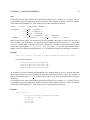
The local referential of a nucleotide, and thus of a nitrogen base, is defined by a Cartesian coordinate system
whose position, relative to the base, can be computed from its atomic coordinates (see Figure 3.1). The
local referential of a nucleotide can be defined arbitrarily, but must be identical for each type of nucleotide.
Let u be the unit vector between coordinates of atom N1 and C2 in pyrimidines, and N9 and C4 in purines.
Let v be the unit vector between coordinates of atom N1 and C6 in pyrimidines, and N9 and C8 in purines.
Then, the unit vector y of the Cartesian coordinate system lies in the direction given by the sum u + v,
the unit vector z is oriented along the cross product u × v, and the unit vector x, following the right hand
rule for a Cartesian coordinate system, is given by y × z. The relative positions of local referentials can be
expressed using homogeneous transformation matrices (HTM), which were first developed in the field of
geometry [20], and later extensively used in computer graphics and robotics. HTMs encode, in the form of a
4x4 matrix, the geometric operations needed to transform objects in 3-D space from one local referential to
another. In the base-base interaction context, a HTM describes the relation by a composition of a translation
and a rotation between the two local referentials of the involved nitrogen bases.
Let Rb1 and Rb2 be the local referentials of nucleotides b1 and b2 as expressed relative to the global
referential centered at the origin, (0, 0, 0). The spatial relation between Rb1 and Rb2 is then given by
the HTM Mb1 →b2 = R−1
b1 Rb2 (see Figure 3.1). In a molecular modeling context such as implemented
in MC-Sym [19], this relation can be reproduced and the atomic coordinates of nucleotide b02 relative to
nucleotide b01 computed by applying the transformation obtained by the matrix product Rb01 Mb1 →b2 R−1
b02
to the absolute atomic coordinates of b02 . In a similar way, the atomic coordinates of b01 relative to b02 can
−1
0
be computed by applying the inverse transformation Rb02 M−1
b1 →b2 Rb0 to the absolute coordinates of b1 . It
1
is worth noting here that M−1
b1 →b2 = Mb2 →b1 , that is the inverse of the transformation extracted between
Rb1 and Rb2 , is equivalent to the one that would have been extracted between Rb2 and Rb1 .
8
9
CHAPTER 3. THE ANNOTATION PROCESS
Rb2 =
[
0.81
-0.11
-0.57
0.00
-0.19
0.88
-0.44
0.00
0.55 46.38
0.47 11.80
0.69 52.25
0.00 1.00
[
z
C2
x
y
N1
C6
z
Mb1
C8
b2
=
y
N9
x
[
0.98
0.07
-0.18
0.00
-0.05
-0.81
-0.59
0.00
-0.18 -3.31
0.59 7.01
-0.79 2.89
0.00 1.00
[
C4
Rb1 =
[
0.71
-0.24
-0.67
0.00
0.53
-0.44
0.72
0.00
-0.46 46.32
-0.87 16.60
-0.18 45.52
0.00 1.00
[
Figure 3.1: Local referentials and base-base relations. Rb1 and Rb2 are the HTMs representing the local
referentials of two nucleotides, b1 and b2 . Mb1 →b2 encodes the relation between Rb1 and Rb2 , that is the
position of Rb2 relative to Rb1 .
3.2 Nucleotide conformations
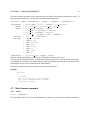
Based on traditional definitions of nucleotide conformations, their symbolic characterization takes place on
two levels. The first one is the position of the furanose ring atoms relative to the general plane of the ring,
which determines the sugar puckering mode. The values of the pseudorotation phase angle for furanose
rings described by Altona et al. [1] are divided into the ten classes shown in Table 3.2. The second is
the orientation of the nitrogen base relative to the sugar, which can be determined by the angle around
the glycosyl bond, χ, defined by the atoms O4’, C1’, N9 and C4 for purines and the atoms O4’, C1’,
N1 and C2 for pyrimidines. As accepted by the IUPAC-IUB commision [12], values of χ in the range
[−90◦ , 90◦ [ indicate a syn orientation whereas other values indicate a trans orientation. Since the other parts
of a nucleotide are mostly rigid, the two above properties represent a fair qualitative description of nucleotide
conformations. The class of a nucleotide conformation can thus be defined by its sugar puckering mode and
nitrogen base orientation around the glycosyl bond. The corresponding symbols assigned by MC-Annotate
are summerized in Table 3.2.
The distance, d(b1 , b2 ), between two nucleotide conformations, b1 and b2 , can be defined by the root
mean square deviation (RMSD) between the heavy atoms in the backbone of the two nucleotides, a posteriori of optimal superimposition of their local referentials in 3-D space [9]. Our metric is in good correlation
with the more standard all-atom superposition and RMSD metric, da (b1 , b2 ), performed using the analytical method described by Kabsch [13, 14] and places the emphasis on the backbone atom positions and
orientation relative to the nitrogen base.
3.3
Base-base interactions
For the classification of base-base interactions, we consider nucleotide pairs that involve at least one of the
known chemical stabilizing forces, that is, covalent binding of adjacent bases, H-bond base pairing and base
stacking. Base-base interactions are thus of five distinct types: adjacent, adjacent-stacked, adjacent-paired,
non-adjacent-stacked and non-adjacent-paired (see Table 3.2). The non-adjacent-non-paired-non-stacked
10
CHAPTER 3. THE ANNOTATION PROCESS
Nucleotide conformation
Set of symbols
1. Type
{A, C, G, U, T}
2. Sugar pucker
{C1'-endo, C1'-exo, C2'-endo, C2'-exo,
C3'-endo, C3'-exo, C4'-endo, C4'-exo,
O4'-endo, O4'-exo}
3. Orientation around
glycosidic bond
{anti, syn}
Base-base interaction
Set of symbols
1. Types
{A, C, G, U, T}2
2. Adjacency
{adjacent, non-adjacent}
3. Stacking
{stacked, non-stacked, helically stacked}
4. Pairing
{paired, non-paired}
a. Relative glycosidic
bond orientation
{cis, trans}
b. Interacting edges
{W, Ww, Ws, Wh, S, Sw, Ss, H, Hw, Hh,
C8, B, Bs, Bh}2
c. MC-Sym number
{I, II, ..., XXVIII, 29, 30, ..., 137}
Figure 3.2: Symbols used in classification. Two symbols from the base type and interacting edges are used,
one for each nucelotide involved in the base-pair as indicated by the exponent 2. The MC-Sym numbers
for base-pairs of two or more H-bonds are in roman, whereas arabic numbers are used for one H-bond
base-pairing patterns.
nucleotide pairs are the most frequent, but they were not considered since they do not involve actual chemical
interactions.
Traditionnal encodings of adjacent base-base interactions uses the six backbone torsion angles α, β, γ,
δ, and ζ [24] or, more recently, the two pseudotorsion angles η and θ [6]. These parameters accurately
describe the relative placement of nucleotides linked by a phosphodiester bond. However, it has already
been observed that distinct torsion angle combinations can result in similar backbone directions and base
orientations. This phenomenon is known as the “crankshaft effect” [11, 22]. Also, non-adjacent base-base
interactions, like base pairings that are stabilized by H-bonds and non-adjacent base-base stacking, cannot
be accurately parameterized using these angles. Rather, a plethora of rotation and translation parameters
have been used to describe these interactions [2, 15, 17]. A simplified and unified encoding scheme for any
type of base-base interactions that emerged from the introduction of HTMs is introduced. In order to allow
us to effectively compare base-base interactions, a distance metric between between two HTMs, Mb1 →b2
and Nb01 →b02 , should possess the following properties:
d(Mb1 →b2 , Nb01 →b02 ) = d(Nb01 →b02 , Mb1 →b2 )
(3.1)
−1
d(Mb1 →b2 , M−1
b1 →b2 ) = 0 ⇐⇒ Mb1 →b2 = Mb1 →b2
(3.2)
d(Mb1 →b2 , Nb01 →b02 ) =
−1
d(M−1
b1 →b2 , Nb01 →b02 )
(3.3)
Equation 3.1 states that the distance metric should obviously be commutative. Equation 3.2 states that a
relation should have a null distance with itself, but not with it’s inverse unless they are equal. Equation 3.3
states that the distance metric should not depend on the direction of application, implicit in the HTM representation. The metric should allow us to discriminate non-directional nucleotide relations.
11
CHAPTER 3. THE ANNOTATION PROCESS
The simple Euclidean distance in the 16 dimensional space of HTMs does not satisfy the above properties since HTMs embed a combination of translation and rotation terms that need to be considered separately.
A HTM can be decomposed in the product of two HTMs, M = TR, where T contains the translation and
R contains the rotation embedded in the original HTM. Paul [23] showed how to extract the length of the
translation, l, as well as the angle θ and the axis of rotation k from matrices T and R. The strength of a
transformation, S(M), regardless of the axis of rotation, is defined by:
s
S(M) =
θ
l2 + ( )2
α
(3.4)
where α represents a scaling factor between the translation and rotation contributions. A scaling factor of
˚ yields to a nice correlation with the RMSD metric, and means that a rotation of 30◦ around any axis
30◦ /A
˚ between two nucleotides’ local referentials. Using this expression, the
is equivalent to a displacement of 1A
distance between two base-base interactions, d(M, N), can be defined by:
d(M, N) =
[S(MN−1 ) + S(M−1 N)]
2
(3.5)
which satisfies the requirements of equations 3.1 to 3.3. In equation 3.5, the composition of transformation
MN−1 can be seen as the necessary transformation needed to align the local referential R0b2 with Rb2
when R0b1 and Rb1 are aligned with the global referential. Similarly, M−1 N can be interpreted as the
transformation required to align R0b1 with Rb1 when R0b2 and Rb2 are aligned with the global referential.
Although HTMs are perfectly suited to uniformely encode base-base interactions, the information they
contain is too compact to identify the type of relations they encode without reproducing the relation in 3-D
space, and evaluating other parameters. For this reason, the symbolic annotations of base-base interactions
are determined from atomic coordinates.
3.4
Base pairing
Hydrogen bonds (H-bonds) are weak electrostatic interactions involving hydrogen atoms located between
two atoms of higher electronegativity. Being weaker than covalent bonds, they are nevertheless the most
significant interactions in the folding and stabilization of DNA and RNA molecules. H-bonds are directional
due to the orbital shape of the electron density distributions, and thus favor planar base pair geometries
formed by at least two H-bonds. Most one H-bond pairings are also planar due to stacking effects within the
helical regions where they are found.
Base pairing between two nucleotides can be determined using the probabilistic method developed in
our group, which yields a symbolic classification of the possible H-bonding patterns.
The classification is based on the involved faces of each base. Here, these faces are divided into many
subfaces that better distinguishes between two pairing types. They were determined from a statistical and
empirical analysis of observed base pairs and the details can be found in an article by Lemieux & Major.
In addition to the face oriented classification of base pairings, identification numbers are used in MCSym. Roman numerals indicate the two (or three) H-bonds pairings identified by Donohue [4, 5] whereas
arabic numerals indicate the bifurcated and single H-bond pairing patterns generated by Gautheret [8]. This
nomenclature was introduced in pre-3.3 versions of MC-Sym and is preserved in newer version for backward
compatibility. Table 3.2 summarizes the different parameters of base pair classification.
CHAPTER 3. THE ANNOTATION PROCESS
12
3.5 Base stacking
Vertical nitrogen base stacking is a significant stabilizing interaction of DNA and RNA 3-D structures,
which plays a major role in their folding and complexation. Stacking occurs more frequently between
adjacent, but also non-adjacent, nucleotides, mostly in double-stranded helical regions. The stabilization
of base stacking involves London dispersion forces [10], and interactions between partial charges within
the adjacent rings [25]. Evidences for hydrophobic forces between bases in solution [27], as well as a
contradictory nonclassical hydrophobic effect [21], have been observed. However, these interactions were
not characterized and parameterized such that they could define precise energy parameters that could be used
for the detection of base stacking [26]. Instead, a geometrical approach was chosen based on the method
proposed by Gabb et al. [7].
We use relaxed ranges of the values defined in the Gabb et al. method to detect base stacking, even
if somewhat large deviations from ideal parameters are observed. It has been shown that there are many
inconsistencies in the atomic coordinates of RNA structures. The deviations measured in NMR spectroscopy
and x-ray diffraction structures can be due to variations in the refinement protocols and force fields, as well
as to artifacts resulting from the determination processes [3, 28].
Therefore, we consider stacking between two nitrogen bases if the distance between their rings is less
˚ the angle between the two normals to the base planes is inferior to 30◦ , and the angle between
than 5.5A,
the normal of one base plane and the vector between the center of the rings from the two bases is less than
40◦ . The class of a stacking interaction is defined by the nucleotides involved in it (Table 3.2).
Chapter 4
Commands reference
4.1 Sequence description
4.1.1
sequence
While writing a MC-S YM script, one musts first specify the sequence he or she is working on. This is done
in the sequence section and it’s usually the first line of a MC-S YM III script. The syntax is the following:
sequence (<type> <residueId> <sequence>+)
<type>
<residueId>
<residueNo>
<sequence>
=
=
=
=
r for RNA or d for DNA.
<chainId><residueNo>
Specify the number of the first residue of the sequence.
The sequence should be entered in uppercase, containing exclusively ’A’, ’C’, ’G’ or ’U’.
This command creates the sequence in memory and prepare it for conformational exploration. It is possible
to use many sequence command to describe different strand or to break down a long strand for the
aesthetic of the script.
Example:
sequence (r A11 GCCAUUUUCGAAUGGC)
4.2
4.2.1
Conformation
residue
The job of assigning conformations to single residues is done by a CDatabaseFG fragment generator. It is a
closed FG and the addressed fragment consists of only one residue. Such a FG is always consistent.
residue (<residueConformation>+)
<residueConformation> =
<residueId> <properties> <set size>
13
14
CHAPTER 4. COMMANDS REFERENCE
The backbone conformation of the residue identified by <residueId> will be assigned conformations described by <properties>. <set size> defines the number of such different conformations that will be tried. A
proportion of the complete <set size> can be specified with the % following the percentage.
<residueConformation> =
<residueId1> [<residueId2>] <properties> <set size>
This syntax is just a short cut for defining several residue (form <residueId1> to <residueId2> inclusively)
that will be assigned identical sets of conformations. The allowed properties for residue conformations are
as defined in Saenger [24] and described in section 5.
Example:
residue
(
A11 A16
A17
A18
A19
A20
A21 A26
)
4.3
4.3.1
{
{
{
{
{
{
helix }
type_A || helix }
C3’_endo && anti }
}
type_A }
helix }
1
10
25
35
10%
100%
Relations between nucleotides
connect
A CTransfoFG fragment generator places a fragment in space (the Target) relatively to an already placed
residue (the Reference ). This is not a closed FG: it depends on the Reference. The Target can be any closed
FG.
connect (<connectDescription>+)
<connectDescription>
=
<residueId1> <residueId2> <properties> <set size>
This command defines the relations that will be used to place residues adjacent in the sequence. If <residueId1>
and <residueId2> are not adjacent, the relation will be applied to each successive pair of residues in the interval. The second rule is used to specify residue specific properties (useful only to specify the residues
faces involved in adjacent pairings).
Example:
connect
(
A11 A16
A16 A19
A19 A20
A20 A21
A21 A26
)
{
{
{
{
{
helix }
stack }
! stack }
stack }
helix }
1
50%
30
20
100%
CHAPTER 4. COMMANDS REFERENCE
4.3.2
15
pair
This command also describes a CTransfoFG and is used to define the relations that will be used to place
residues not adjacent in the sequence. Typically, the relation will involve hydrogen bond between the bases.
Base pairings are described using the operator ’/’ which takes two operands, the former applying to the first
residue in the statement and the latter applying to the second.
pair (<pairDescription>+)
<pairDescription> =
<residueId1> <residueId2> <properties> <set size>
An example would be:
Example:
pair
(
A12 A26 { W / H pairing cis } 10
)
where this means that we are looking for pairings involving the Watson-Crick edge of A12 and the
Hoogsteen egde of A26. Some other examples:
Example:
pair
(
A11 A26 { wct }
100%
A12 A25 { wct }
100%
A13 A24 { wct }
100%
A14 A23 { wct }
1
A15 A22 { wct }
1
A16 A21 { cis && W / W }
1
A17 A20 { trans && S / H }
25
A1 A6 { Ww / Ww && strong }
5
A2 A5 { Ww / any && strong }
5 // any means any faces for A5
A3 A4 { Hh / (Ww || Hh) && strong } 3
B1 B9 { (Ww / Ww && cis) || (Ww / H && trans) } 3
)
4.4
Building information
The building information is used to instruct MC-S YM on how to place the nucleotides. In its most basic
form, it only contains a backtrack statement that defines the order of nucleotides placement. The cache
statement is used most of the time and allows to filter out similar structures based on a RMSD criterion.
CHAPTER 4. COMMANDS REFERENCE
4.4.1
16
backtrack
This statement defines a CBacktrackFG fragment generator responsible for the placement in space of all
fragments contained in it’s declaration using a backtracking algorithm.
<name> = backtrack ([<fragmentGenerator>] <buildSequence>+)
<buildSequence> =
=
(<referenceResidue> <placedResidue>*))
place (<referenceResidue> <placedResidue> <fragmentGenerator>)
The backtrack keywork is used to define the order in which the bases will be placed. The <fragmentGenerator> variable can refer to any named fragment generator described in the current section.
Example:
hairpin = backtrack
(
(A11 A26)
(A11 A12 A25)
)
4.4.2
cache
A Cache is used to keep in memory some sub-structures that have already been generated to reduce redundant processing. It is generally attached to a backtrack fragment generator. It is possible to reduce the
number of cache-saved structures by eliminating any new structure that is too similar to the previously generated ones. This allows one to avoid generating plenty of equivalent models and greatly facilitates results
analysis. The selection algorithm performs Root Mean Square (RMS) alignment of any new structure with
all cache-saved models and for each comparison, it returns the RMS deviation. Any value smaller than a
user-set RMSD bound will cause the new model to be rejected. The basic idea behind this algorithm is to
minimize the differences between the coordinates of corresponding atoms by doing a set of translations and
rotations of the “fit” set.
Typical values of the RMSD bound are in the range [ 0.0, 5.0 ].
Extensive use of cache objects while modeling large molecules causes the memory needed by the program to
grow very rapidly. It is advisable to limit excessive cache growth by an appropriate RMSD bound. This will
avoid unecessary virtual memory swapping (or even overflow) and will considerably decrease the execution
time.
<name1> = cache (<name> <filter function>)
<filter function>
<atomset>
= rmsd (<bound> [align] [<atomset>] [no hydrogen])
= all | base only | backbone only | pse only
bound the rmsd lower bound;
align If this options is chosen, any new structure to be added to the cache will be first aligned to the most
similar structure already in the cache;
atomset One can choose the atoms on which the RMSD comparison algorithm will be applied. The following mutually exclusive options are available: all, base only, backbone only and pse only
CHAPTER 4. COMMANDS REFERENCE
17
(the PSE atoms are artificial atoms arbitrarily placed on each base for computational purposes). One
can also add the useful no hydrogen option.
Example:
hairpin_cache = cache
(
hairpin
rmsd (1.0 base_only no_hydrogen)
)
4.4.3
library
A library object is used to modify an entire fragment by using a pre-defined database, or library. That predefined database consist of a set of files, all formatted the same way, and each describing a possible structure
for that fragment. One can seek models for large molecules by first constructing libraries for different
fragments of the entire structure. Those libraries can be efficiently built by using MCSYM independently on
each fragments.
The main objective behind the creation of the library object is quite similar to that of the cache object: we
wanted to save the exponential processing time lost when generating more than once the same sub-structures
on different edges of the backtrack tree.
For optimisation purposes, the algorithm assumes that all files of the same library are formatted exactly
the same way (the first file in the set is used as a reference for the entire library. This means that residues
must be defined in the same order in every file.
Before using a library object, one must specify the files constituting the library. For now, only three type
of files are available: the PDB format, the binary format and through socket. All input files must be named
exactly the same way, i.e. <name><number><suffix>; the number must be encoded in a C format.
File numbers must begin at 1 and must be consecutive.
Example:
anticodon-00001.pdb.gz
anticodon-00002.pdb.gz
anticodon-00003.pdb.gz
anticodon-00004.pdb.gz
...
change id
As the Libraries are usally constructed independently of the main modeling project, it is frequent that chain
IDs of loaded residues do not correspond to the chain IDs of the main project’s residues. It is possible to
specify new chain IDs for the loaded residues (if you don’t, the program will not recognize the library).
CHAPTER 4. COMMANDS REFERENCE
18
strip
It is possible to ignore some residues that are present in the library files by using the strip option. The user
is responsible to properly handle those residues with some other fragment generators. This is for example
useful when careful handling of a “joint” between two or more fragments is required.
<name> = library ( <input form> <modifier>* )
<input form> =
=
=
=
<modifier> =
file pdb ("<Cformat>")
file bin ("<Cformat>")
file rnaml ("<File name>")
socket bin ("<address>" <port> "<Cformat>")
strip( <residue>+ ) | change id( "<char1>" , "<char2>" )
Before using a library object, one must specify the files constituting the library. For now, only one type of
files is available: the PDB format. All input files must be named exactly the same way, i.e. a name that
works as a C format string. A filename may be given followed by a “counter” so that increasing the counter
will produce a new filename, i.e. "anticodon-%04d.pdb" where "%04d" (the counter) means that the
number will be four digits long and padded with “0”. File numbers must begin at 1 and must be consecutive.
Example:
antic_lib = library (file_pdb ("/home/foo/ANTI/anticodon-%04d.pdb"))
will lead to these filenames:
/home/foo/ANTI/anticodon-0001.pdb
/home/foo/ANTI/anticodon-0002.pdb
/home/foo/ANTI/anticodon-0003.pdb
/home/foo/ANTI/anticodon-0004.pdb
...
As the libraries are usally constructed independently of the main modeling project, it is frequent that chain
IDs of loaded residues do not correspond to the chain IDs of the main project’s residues. It is possible to
specify new chain IDs with chain id for the loaded residues (if you don’t, the program will not recognize
the library).
It is possible to ignore some residues that are present in the library files by using the strip option. The user
is responsible to properly handle those residues with some other fragment generators. This is for example
useful when careful handling of a “joint” between two or more fragments is required.
Example:
kiss = library
(
file_pdb ("/home/foo/PDB/kiss-%05d.pdb")
change_id (" ", "B")
strip (A37)
strip (A51)
strip (A60)
)
CHAPTER 4. COMMANDS REFERENCE
19
4.5 Constraints
4.5.1
Adjacency
This command will create distance constraints between atoms O3’ and P of adjacent residues addressed by
the build order defined by <name>. Since MC-S YM places nucleotides using nitrogen base relations, this
constraint is needed to insure that the backbone is closing within reasonnable boundaries.
adjacency (<name> <lower bound> <upper bound>)
Example:
adjacency (hairpin 1.0 3.0)
4.5.2
Angle
This command will create a constraint with the angle formed by the three atoms. The central atom is where
the angle is placed. The <min angle> and <max angle>, in degrees, specifies the range of accepted values
(0 ¡= angle ¡= 180).
angle (<angleConstraint>+)
<angleConstraint>
<atom>
= <atom> <atom> <atom> <min angle> <max angle>
= <residue> : <atomName>
Example:
angle
(
A10:O3’ A11:P A11:O5’ 100 130
A11:O3’ A12:P A12:O5’ 100 130
)
4.5.3
Residue clash
This command will implement a hard-sphere potential to reject structure containing atoms closer than the
lower bound. If no option is used, the default is to check the constraint for all atoms, including hydrogens.
res clash (<name> [fixed distance | vdw distance]
<lower bound> [<option>] [no hydrogen])
<option> =
all | base only | backbone only | pse only
Example:
res_clash
(
hairpin
fixed_distance 1.0
all
no_hydrogen
)
CHAPTER 4. COMMANDS REFERENCE
4.5.4
20
Distance
distance (<distanceConstraint>+)
<distanceConstraint> =
<atom> =
<atom1> <atom2> <lower bound> <upper bound>
<residue> : <atomName>
Example:
distance (1:C1’ 4:C1’ 1.0 10.0)
4.5.5
Relation
To impose a harder constraint on model building, one might want to close a cycle. Until now, such a
construction was not possible with mcsym: no cycle where permitted in the construction order. With the
addition of the relation constraint a modelisator can close a cycle with this new constraint.
Be aware that the constraint should be used only when you cannot build a relation via the pair (not
adjacent) / connect (adjacent) statements. Both do the same thing but the pair and connect statements reduce
the search space before exploration, which is much less costly than using the relation constraint.
relation (<relationConstraint>+)
<relationConstraint>
= <res1> <res2> <properties>
Example:
relation
(
42 43 {
41 42 {
40 41 {
39 40 {
)
4.5.6
stack
stack
stack
stack
}
}
}
}
Torsion
This command will create a constraint on the torsion angle formed by the two first and the two last atoms.
The <min angle> and <max angle>, in degrees, specifies the range of accepted values (-180 ¡= torsion angle
¡= 180).
torsion (<torsionConstraint>+)
<torsionConstraint>
<atom>
= <atom> <atom> <atom> <atom> <min angle> <max angle>
= <residue> : <atomName>
Example:
torsion (42:O3’ 43:P 43:O5’ 43:C5’ -67.9 -67.6)
CHAPTER 4. COMMANDS REFERENCE
21
4.6 Exploration of the conformational space
4.6.1
explore
explore (<name> [<filter function>] [<option>])
<filter function>
<atomset>
<option>
=
=
=
=
=
=
rmsd (<float> [align] [<atomset>] [no hydrogen])
all | base only | backbone only | pse only
file pdb ("<Cformat>" [zipped])
file rnaml ("<File name>" [zipped])
file bin ("<Cformat>" [zipped])
socket bin ("<address>" <port> "<Cformat>")
The filter sub-statement builds a special cache for filtering the structures to be saved.
The only present filtering function is a rmsd function that compares the new solution with the cached ones.
It’s arguments are the rmsd lower bound, an flag to align the candidate structure with it’s best match in the
cache and the atom sets to be considered in the rmsd function.
The optional zipped keyword will enable the compression of output files.
Example:
explore
(
trna_phe
rmsd (1 align base_only no_hydrogen)
file_pdb ("PDB/helix-%03d.pdb" zipped)
)
4.6.2
exploreLV
Instead of systematically trying every possible conformation for each residue, this probabilistic algorithm
takes a random conformation for each residue. If this random choice of conformations satisfies every given
structural constraints, the probabilistic algorithm has succeeded in finding a complete valid tertiary structure
for the molecule. It will save this correct solution and make another set of random choices for each residues
conformation. If the random choices doesnt satisfy every constraints, the current solution is simply ignored
and probabilistic exploration continues with a new set of random conformations. This Las Vegas probabilistic algorithm doesnt achieve an exhaustive tertiary structures exploration. It randomly find a subset of every
possible tertiary structures for a molecule. However, non-exhaustive probabilistic exploration has a major
advantage over exhaustive exploration by backtrack, that is its higher valid structures finding rate. Actually,
probabilistic exploration succeed more rapidly in finding a correct path from the implicit tree root to one of
its leaves. Even if this probabilistic approach to explore a molecules tertiary structures seems quite naive,
it has the benefit of never become trapped in an excessively fastidious and useless exploration of a sterile
sub-tree due to a shallower residue conformation. A consequence for this approach is that valid tertiary
structures are generated independently, so theres more diversity in a given set of tertiary structures explored
by a Las Vegas algorithm than by a backtrack algorithm. In fact, the chances are that a newly found tertiary
structure by probabilistic exploration will be totally different from its predecessor, which aint the case in
exploration by backtrack.
CHAPTER 4. COMMANDS REFERENCE
22
The cache fragment generators in the exploration tree are disable when using the probabilistic search. To
filter the generated structures, use the cache sub-statement described below.
exploreLV (<name> [<filter function>] [<option>] [<time limit>] [<backtrack size>])
<filter function>
<atomset>
<option>
<time limit>
<time limits>
<backtrack size>
=
=
=
=
=
=
=
=
=
=
=
=
=
=
=
=
rmsd (<float> [align] [<atomset>] [no hydrogen])
all | base only | backbone only | pse only
file pdb ("<Cformat>" [zipped])
file rnaml ("<File name>" [zipped])
file bin ("<Cformat>" [zipped])
socket bin ("<address>" <port> "<Cformat>")
time limit (<time limits>+)
<integer> seconds
<integer> sec
<float> minutes
<float> min
<float> hours
<float> hr
<float> days
<float> d
backtrack size (<integer> <integer>)
The filter sub-statement builds a special cache for filtering the structures to be saved.
The only present filtering function is a rmsd function that compares the new solution with the cached ones.
It’s arguments are the rmsd lower bound, an flag to align the candidate structure with it’s best match in the
cache and the atom sets to be considered in the rmsd function.
The optional zipped keyword will enable the compression of output files.
Example:
exploreLV
(
anticodon
rmsd (1 align base_only no_hydrogen)
file_rnaml ("PDB/helix.xml" zipped)
time_limit (1 days)
)
4.7
4.7.1
Miscellaneous commands
source
source ("<filename>")
This command reads a MC-S YM script file identified by <filename> and evaluates it within the interpretor.
CHAPTER 4. COMMANDS REFERENCE
4.7.2
23
restore
restore (<status filename> [<option>])
<status filename> =
<option> =
=
=
the status filename between double quores
file pdb ("<Cformat>" [zipped])
file bin ("<Cformat>" [zipped])
socket bin ("<address>" <port> "<Cformat>")
The optional zipped keyword will enable the compression of output files.
Restores the mcsym status file and continue the exploration. The status file is saved every 30 minutes in
the MCSYM CACHE DIR directory under the name of the explored fragment generator with the process id
(PID) and the .msf extension. It contains sufficient informations to restart the structure exploration in case
of an interruption.
Example:
restore
(
"/home/user1/mcsym/theCache-123.msf"
file_pdb ("PDB/helix-%03d.pdb" zipped)
)
4.7.3
notes
notes
Prints the available comments from the database.
4.7.4
remark
remark ("<comment>")
The <comment> will be added in the REMARK section of all generated pdb files.
4.7.5
reset
reset
This command will disable all previously entered commands.
4.7.6
version
version
Prints the MC-S YM version.
4.7.7
quit
quit
Ends the MC-S YM session.
CHAPTER 4. COMMANDS REFERENCE
4.7.8
24
Comments
// This is a comment
Comments can be included in the script by the use of the // keyword. Every character following this
keyword until the end of the line will be ignored.
Chapter 5
Database properties reference
5.1 Properties
{[<expression>]}
<expression>
<and expression>
<or expression>
<face expression>
<not expression>
<base expression>
=
=
=
=
=
=
=
=
<and expression>
<or expression> [&& <and expression>]
<face expression> [|| <or expression>]
<not expression> [<not expression> / <not expression>]
! <not expression>
<base expression>
<property>
( <expression> )
The <expression> is a boolean test that will accept or reject a conformation or a relation. The field may be
empty, in that case every conformation or relation will be accepted whatever properties it has. With this kind
of expression you can restrict your sets of conformations or relations without specifying all the elements.
Per example:
Example:
{ saenger && ! ( XXII || XIX ) }
will give you a set of all Saenger relations without types XXII and XIX.
5.2
Conformational properties of the residue
Properties describing the pucker mode:
C1’
C1’
C3’
O4’
endo
exo
endo
endo
O4’ exo
C2’ exo
C4’ exo
C2’ endo
C3’ exo
C4’ endo
25
CHAPTER 5. DATABASE PROPERTIES REFERENCE
26
Properties describing the glycosyl bond: anti, syn
Others conformation properties:
type A → C3’ endo and anti
type B → C2’ endo and anti
helix → Conformation used to build standard A-form helix.
For the residues, using an empty properties list ( { } ) means that any type of conformation will be tested.
5.3
Properties of the relation between two residues
Properties of relations involving a O3’-P covalent bond:
stack → Stacking
nostack → No stacking (deprecated, use !stack)
reverse → Reverse stacking
connect → Any covalently bonded relation (stack+!stack) (deprecated, use adjacent)
helix → Standard A-Form double helical stacking
Properties of relations for paired residues:
pairing
<I to XXVIII>
saenger
<29 to 137>
one hbond
theo
cis
trans
wct
→ All pairing interaction
→ Pairing described by Saenger
→ All of the above
→ One-H-bond pairings described by Gautheret
→ All of the above One-H-bond
→ Only theoretical (planar) pairing
→ Glycosyl bonds are in the same orientation relative to the mean
orientation of H-bonds
→ Glycosyl bonds are in opposite orientation relative to the mean
orientation of H-bonds
→ Watson-Crick pairing used to build standard A-form helix
CHAPTER 5. DATABASE PROPERTIES REFERENCE
Properties of residues in paired relations:
any
W
Ww
Wh
Ws
H
Hh
Hw
C8
S
Sw
Ss
B
Bs
Bh
→
→
→
→
→
→
→
→
→
→
→
→
→
→
→
any of the residue faces involved
Watson-Crick face involved: (Ww || Wh || Ws)
center of the Watson-Crick face involved
Watson-Crick face involved, near the Hoogsteen face
Watson-Crick face involved, near the Sugar face
Hoogsteen face involved: (Hw || Hh || C8)
center of the Hoogsteen face involved
Hoogsteen face involved, near the Watson-Crick face
Hoogsteen face involved, near the C8 atom
Sugar face involved: (Sw || Ss)
Sugar face involved, near the Watson-Crick face
center of the Sugar face involved
Bifurcated face involved
Bifurcated face involved, near the Sugar face
Bifurcated face involved, near the Hoogsteen face
27
Chapter 6
A complete example: The tRNA Anticodon
stem loop Script
This section contains a complete MC-S YM III script for the modeling of the anticodon stem-loop of the
tRNA. This example also acted as a bench mark for testing during development of MC-S YM III.
//
//
//
//
//
//
//
//
//
//
-*- Mode: Mcsym -*anticodon.mcc
c 2000 Laboratoire de Biologie Informatique et Th´
Copyright eorique.
Author
:
Created On
:
Last Modified By : Martin Larose
Last Modified On : Mon Mar 27 16:52:08 2000
Update Count
: 1
Status
: Ok.
// Script MC-Sym 3 pour la boucle anticodon du trna
//
//
3
123456789
sequence (r 31 ACUGAAGAU)
// Conformations ------------------------------------------residue
(
31
39
32 38
)
{ helix }
1
{ helix }
1
{ type_A } 15
// Relations -----------------------------------------------
28
CHAPTER 6. A COMPLETE EXAMPLE: THE TRNA ANTICODON STEM LOOP SCRIPT
connect
(
31 33
33 34
34 39
)
pair (31
{ stack }
{ ! stack }
{ stack }
39
20
20
20
{ wct } 1)
// Building -----------------------------------------------anticodon = backtrack
(
(31 39)
(39 38 37 36 35 34)
(31 32 33)
)
// Constraint ---------------------------------------------adjacency (anticodon 1.0 2.5)
res_clash
(
anticodon
fixed_distance 1.0
all
no_hydrogen
)
// Exploration --------------------------------------------explore
(
anticodon
rmsd (1.0 base_only no_hydrogen)
file_pdb ("ANTI/anti-%04d.pdb" zipped)
)
29
Appendix A
Base pairings classification
30
Bibliography
[1] C. Altona and M. Sundaralingam. Conformational analysis of the sugar ring in nucleosides and nucleotides. a new description using the concept of pseudorotation. J. Am. Chem. Soc., 94:8205–8212,
1972. 3.2
[2] M.S. Babcock, E.P.D. Pedneault, and W.K. Olson. Nucleic acid structure analysis. J. Mol. Biol.,
237:125–156, 1994. 3.3
[3] R.E. Dickerson, K. Grzeskowiak, M. Grzeskowiak, M.L. Kopka, T. Larsen, A. Lipanov, G.G. Priv´e,
J. Quintana, P. Schultze, K. Yanagi, H. Yuan, and H.-C. Yoon. Polymorphism, packing, resolution, and
reliability in single-crystal DNA oligomer analyses. Nucleosid. Nucleotid., 10:3–24, 1991. 3.5
[4] J. Donohue. Hydrogen-bonded helical configurations of polynucleotides. Proc. Natl. Acad. Sci. (USA),
42:60–65, 1956. 3.4
[5] J. Donohue and K.N. Trueblood. Base pairing in DNA. J. Mol. Biol., 2:363–371, 1960. 3.4
[6] C.M. Duarte and A.M. Pyle. Stepping through an RNA structure: A novel approach to conformational
analysis. J. Mol. Biol., 284(5):1465–1478, 1998. 3.3
[7] H.A. Gabb, S.R. Sanghani, C.H. Robert, and C. Pr´evost. Finding and visualizing nucleic acid base
stacking. J. Mol. Graphics, 14:6–11, 1996. 3.5
[8] D. Gautheret and R.R. Gutell. Inferring the conformation of RNA base pairs and triples from patterns
of sequence variation. Nucl. Acids Res., 25(8):1559–1564, 1997. 3.4
[9] D. Gautheret, F. Major, and R. Cedergren. Modeling the three-dimensionnal structure of RNA using
discrete nucleotide conformationnal sets. J. Mol. Biol., 229:1049–1064, 1993. 1.4.4, 3.2
[10] S. Hanlon. The importance of london dispersion forces in the maintenance of deoxyribonucleic acid
double helix. Biochem. Biophys. Res. Commun., 23:861–867, 1966. 3.5
[11] S.R. Holbrook, J.L. Sussman, R.W. Warrant, and S.-H. Kim. Crystal structure of yeast phenylalanine
transfer RNA, II: Structural features and functional implications. J. Mol. Biol., 123(4):631–660, 1978.
3.3
[12] IUPAC-IUB Joint Commission on Biochemical Nomenclature. Abbreviations and symbols for the
description of conformations of polynucleotide chains. Eur. J. Biochem., 131:9–15, 1983. 3.2
31
BIBLIOGRAPHY
32
[13] W. Kabsch. A solution for the best rotation to relate two sets of vectors. Acta Crystallogr., A32:922–
923, 1976. 3.2
[14] W. Kabsch. A discussion of the solution for the best rotation to relate two sets of vectors. Acta
Crystallogr., A34:827–828, 1978. 3.2
[15] R. Lavery and H. Sklenar. The definition of generalized helicoidal parameters and of axis curvature
for irregular nucleic acids. J. Biomol. Str. Dynam., 6(1):63–91, 1988. 3.3
[16] F. Leclerc, R. Cedergren, and A.E. Ellington. A three-dimensional model of the rev-binding element
of HIV-1 derived from analyses of aptamers. Nature Struct. Biol., 1:293–300, 1994. 1.4.4
[17] F. Leclerc, J. Srinivasan, and R. Cedergren. Predicting RNA structures: the model of the RNA element
binding rev meets the NMR structure. Fold. Des., 2(2):141–147, 1997. 3.3
[18] F. Major, D. Gautheret, and R. Cedergren. Reproducing the three-dimensional structure of a tRNA
molecule from structural constraints. Proc. Natl. Acad. Sci. (USA), 90:9408–9412, 1993. 1.4.4
[19] F. Major, M. Turcotte, D. Gautheret, G. Lapalme, E. Fillion, and R. Cedergren. The combination of symbolic and numerical computation for three-dimensional modeling of RNA. Science,
253(5025):1255–1260, 1991. 1.4.4, 3.1
[20] E.A. Maxwell. Methods of Plane Projective Geometry Based on the Use of General Homogeneous
Coordinates. Cambridge University Press, Cambridge, England, 1946. 3.1
[21] L.F. Newcomb and S.H. Gellman. Aromatic stacking interactions in aqueous solution: Evidence that
neither classical hydrophobic effects nor dispersion forces are important. J. Am. Chem. Soc., 116:4993–
4994, 1994. 3.5
[22] W.K. Olson. Computational studies of polynucleotide flexibility. Nucl. Acids Res., 10:777–787, 1982.
3.3
[23] R.P. Paul. Robot Manipulators: Mathematics, Programming and Control. MIT Press, Cambridge,
1981. 3.3
[24] W. Saenger. Principles of Nucleic Acid Structure. Springer-Verlag, New York, USA, 1984. 3.3, 4.2.1
[25] A. Sarai, J. Mazur, R. Nussinov, and R.L. Jernigan. Origin of DNA helical structure and its sequence
dependence. Biochem., 27(22):8498–8502, 1988. 3.5
[26] J. Sponer and J. Kypr. Theoretical analysis of the base stacking in DNA: Choice of the force field and
comparison with the oligonucleotide crystal structure. J. Biomol. Str. Dynam., 11(2):277–292, 1993.
3.5
[27] I. Tazawa, T. Koike, and Y. Inoue. Stacking properties of a highly hydrophobic dinucleotide sequence,
N6, N6-dimethyladenylyl(3’ leads to 5’)N6, N6-dimethyladenosine, occurring in 16–18-S ribosomal
RNA. Eur. J. Biochem., 109(1):33–38, 1980. 3.5
[28] H. Weissig and P.E. Bourne. An analysis of the protein data bank in search of temporal and global
trends. Bioinformatics, 15(10):807–831, 1999. 3.5