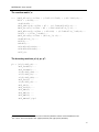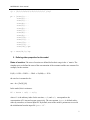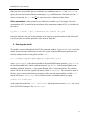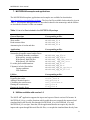
Download MATSEDLAB (v 1.0) – User manual

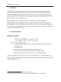
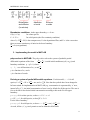
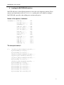
MATSEDLAB – User manual MATSEDLAB (v 1.0) – User manual
Version 1.0
March 1st, 2013
Babak Shafei ([email protected])
Raoul-Marie Couture ([email protected])
Numbers Zhengkai Tu ([email protected])
Philippe Van Cappellen ([email protected])
This software is still under development.
Updates, examples and walkthrough are posted on our website at:
https://uwaterloo.ca/ecohydrology/software.
1 MATSEDLAB – User manual MATSEDLAB – User manual ...................................................................................................... 1
1.
Overview ............................................................................................................................... 3
2.
Theoretical model ................................................................................................................ 3
Diagenesis equation: ................................................................................................................. 3
Boundaries conditions: .............................................................................................................. 4
3.
Implementing the model in MATLAB ................................................................................. 4
pdepe solver in MATLAB ........................................................................................................... 4
Deriving a system of partial differential equations ..................................................................... 4
4.
Locating the MATSEDLAB matrices .................................................................................. 5
The transport matrix, f: .............................................................................................................. 5
The reaction matrix, s: ............................................................................................................... 6
The boundary matrices, pl, ql, pr, qr: ......................................................................................... 6
5.
Defining other properties for the model ............................................................................ 7
Rates of reaction ....................................................................................................................... 7
Other parameters ...................................................................................................................... 8
6.
Running the model .............................................................................................................. 8
7.
Utilities available with version 1.0...................................................................................... 9
Plotting the results: .................................................................................................................. 10
Saving the results .................................................................................................................... 10
Export the results into an EXCEL spreadsheet ....................................................................... 11
Add a species into the model .................................................................................................. 11
Calculating and plotting the rate of reactions .......................................................................... 11
Calculating the fluxes .............................................................................................................. 12
8.
Potential problems and troubleshooting......................................................................... 12
Time integration failed ............................................................................................................. 12
Segmentation violation ............................................................................................................ 12
Long running time: ................................................................................................................... 12
Specific worksheet not found .................................................................................................. 13
DAE of index greater than 1 .................................................................................................... 13
9.
References cited ................................................................................................................ 14
2 MATSEDLAB – User manual 1. Overview
MATSEDLAB is a biogeochemical model, which calculates the concentration of different
species at each depth for a specific time period, based on the reaction framework, transport
processes, and boundary conditions specified by the users. It does so by forming a system of
partial differential equations based on the early diagenesis equation, and using the MATLAB
built-in solver pdepe to solve the system.
MATSEDLAB is executed through the MATLAB home screen. The execution of
MATSEDLAB requires a Windows PC with an active installation of MATLAB (Version 7.6
release R2008a or later1) and MS Excel (Version 2007 or later). It is recommended to allow at
least 1GB of space on the hard drive for the model output and 1GB of contiguous random-access
memory for the initialization routine.
2. Theoretical model
Diagenesis equation2:
where ԑ is the porosity (no units)
C is the concentration of the species (µmol/g for solid and µmol/cm3 for solute)
t is the time (yr)
x is the depth (cm)
D is the coefficient for diffusion and bioturbation (cm2/yr)
ϑ is the rate of burial (for solid) or advection (for solute) (cm/yr)
R is the any sources or sinks for the species (e.g. chemical reactions)
To put the equation in words, the rate of change of concentration is a result of transport (the
terms in the square bracket) and reactions. When the porosity is depth-independent, the equation
can be simplified to give
1
2
MATSEDLAB was developed in and tested up to release R2011b. Aguilera et al. 2005. Symbols have been modified to be consistent with those used in MATLAB 3 MATSEDLAB – User manual Bioturbation
and diffusion
(for solutes)
Advection
or burial
Sources
or sinks
Boundaries conditions: At the upper boundary, x = 0 cm:
C(0,t) = C0(t)
for solute species
f = -J / Fcon
for solid species (the flux continuity condition)
where f (=D
ϑC) is the transport term, J is the depositional flux, and Fcon is the conversion
factor to ensure consistency of units.At the lower boundary:
0 (zero gradients)
3. Implementing the model in MATLAB
pdepe solver in MATLAB: The pdepe solver solves the system of parabolic partial
differential equations of the form
f
c
swith initial condition u(x,0) = u0(x) and
boundary conditions p + qf = 0, where:
c, f, s are all functions of x, t, u and
.
p is a function of x, t and u
q is a function of x and t
Deriving a system of partial differential equations: For this model, c = 1 for all
species, f
D
ϑC
D
wu, and s = ∑ R. Note that the symbols have been changed to
be better suited for implementation in MATLAB (e.g. concentration is represented by ‘u’ now,
instead of by ‘C’). An initial concentration of zero is set by default for all the species. The user is
free to decide for the desired initial concentration according to his needs. For the upper
boundary:
p = u, q = 0 for solute species, so that u + 0 * f = u = 0
p = J/F, q = 1 for solid species, so that J/F f = 0
For the lower boundary:
p = wu, q = 1 for solid species, so that wu + D
wu = D
=0
As such, all the c, f, s, p and q matrices can be defined in MATLAB.
4 MATSEDLAB – User manual 4. Locating the MATSEDLAB matrices
MATSELAB relies on the following matrices to solve the early diagenetic problem. These
matrices are found in the m-file MATSEDLAB.m, and they have to be edited to configure
MATSEDLAB, especially when adding new reactions and species.
Names of the species, VarNames:
VarNames = {'O2(aq)',...
%u1
'Fe(OH)3(s)',... %u2
'FeOOH(s)', ...
%u3
'SO4(2-)(aq)', ...%u4
'Fe(2+)(aq)', ... %u5
'S(-II)(aq)',... %u6
'FeS(s)',...
%u7
'S(0)(aq)',...
%u8
'S8(s)',...
%u9
'FeS2(s)',...
%u10
'OMS(s)',...
%u11
'OM1(s)',...
%u12
'OM2(s)',...
%u13
'OMSO(s)'};
%u14
The transport matrix, f:
f =
[(D_bio+D_O2)*DuDx(1)-w*u(1);...
D_bio*DuDx(2)-w*u(2);...
D_bio*DuDx(3)-w*u(3);...
(D_bio+D_SO4)*DuDx(4)-w*u(4);...
(D_bio+D_Fe)*DuDx(5)-w*u(5);...
(D_bio+D_H2S)*DuDx(6)-w*u(6);...
D_bio*DuDx(7)-w*u(7);...
(D_bio+D_S0)*DuDx(8)-w*u(8);...
D_bio*DuDx(9)-w*u(9);...
D_bio*DuDx(10)-w*u(10);...
D_bio*DuDx(11)-w*u(11);...
D_bio*DuDx(12)-w*u(12);...
D_bio*DuDx(13)-w*u(13);...
D_bio*DuDx(14)-w*u(14)];%f 5 MATSEDLAB – User manual The reaction matrix1, s:
s = [(BC0_O2-u(1))*alfax + (-2*R5-0.25*R6) + (-R1-3*R9)*F;...
R6/F + (-4*R2);...
-4*R3+4*R9;...
(BC0_SO4-u(4))*alfax + R5 + (-0.5*R4+R12-R13)*F;...
(BC0_Fe-u(5))*alfax - R6 + (4*R2+4*R3+R7-R_7)*F;...
(BC0_H2S-u(6))*alfax + (-R5-R10) + (0.5*R4+R7-R_7-R8)*F;...
-R10/F + (-R7+R_7-4*R9);...
(BC0_S0-u(8))*alfax + (R11-R_11)*F;...
+4*R9-R11+R_11;...
+R10/F;...
+R8+R13;...
-R1a-R2a-R3a-R4a;...
-R1b-R2b-R3b-R4b;...
-R12];%s
The boundary matrices, pl, ql, pr, qr2:
pl = [ul(1)-BC0_O2;...
BC0_FeOH3/F;...
BC0_FeOOH/F;...
ul(4)-BC0_SO4;...
ul(5)-BC0_Fe;...
ul(6)-BC0_H2S;...
BC0_FeS/F;...
ul(8)-BC0_S0;...
BC0_S8/F;...
BC0_FeS2/F;...
BC0_OMS/F;...
BC0_OM1/F;...
BC0_OM2/F;...
BC0_OMSO/F];%pl
1
2
The conversion factor F is used to ensure unit consistency between reaction rates with different units. The ‘l’ and ‘r’ here correspond to ‘left’ (upper) boundary and ‘right’ (lower) boundary. 6 MATSEDLAB – User manual ql = [0;1;1;0;0;0;1;0;1;1;1;1;1;1];%ql
pr = [w*ur(1);...
w*ur(2);...
w*ur(3);...
w*ur(4);...
w*ur(5);...
w*ur(6);...
w*ur(7);...
w*ur(8);...
w*ur(9);...
w*ur(10);...
w*ur(11);...
w*ur(12);...
w*ur(13);...
w*ur(14)];%pr
qr = ones(14,1);%qr
5. Defining other properties for the model
Rates of reaction: The rates of reaction are defined before their usage in the ‘s’ matrix. The
simplest rates are defined in terms of the concentration of the reactants and the rate constant. For
example, for the reaction:

Fe(II) + 0.25O2 + 2HCO3 + 2H2O  Fe(OH)3(s) + 2CO2
the rate law is assumed to be :
rate = kfeox [Fe(II)] [O2]
In the model, this is written as:
R5 = ktsox * u(6) * u(1);
where R5 is the arbitrary index for the reaction, u(6) and u(1) corresponds to the
concentration of Fe ions and oxygen respectively. The rate constant, ktsox, is defined earlier,
either by a number, or from an input file. By default, most of the model’s parameters are read at
the initialisation from the input file “para.in”.
7 MATSEDLAB – User manual Other rate laws are possible; the user could also use conditions such as ‘if’ and ‘switch’, to
specify the rate laws under different circumstances, e.g. at different time. Note that since the ‘s’
matrix is a function of x, t, u and
, the rates have to be a function of those alone.
Other parameters: Other parameters are defined in a similar way. For example, since the
concentration of H+ is needed in the calculation of the saturation constant of FeS, it is defined in
the code as:
h_plus = 3.4e-4; %[H+] concentration equals 10^(-pH)
Note that while the user can set the parameter to be equal to a specific number in the code itself,
it is also possible to read the parameter value from an input file.
6. Running the model
The model is executed through the MATLAB command window. Type ‘MATSEDLAB’ to run the
model. It may take up to half an hour to solve the system of partial differential equations, and
store the solution matrix in the global variable ‘sol’:
sol = pdepe(0,@pdex14pde,@pdex1ic,@pdex1bc,x,t);
where: @pdex14pde is the function handle to the partial differential equations, @pdex1ic is
the function handle to the initial condition functions, @pdex1bc is the function handle to the
boundary condition functions, x is the spatial domain, and t is the time domain. The solution
matrix will also be stored in a global cell matrix called ‘SimValues’. The cell matrix, most of
the time, gives a neater and cleaner presentation of the concentrations. Both the variable ‘sol’
and the cell matrix ‘SimValues’ are accessible from the command window by typing:
global sol SimValues
At the end of the model run, ‘sol’, ‘SimValues’ and the parameter matrix ‘para’ are saved
to the MATLAB workspace file ‘Result.mat’.
8 MATSEDLAB – User manual 7. MATSEDLAB examples and applications
The MATSEDLAB template, applications and examples are available for download at:
https://uwaterloo.ca/ecohydrology/software. The list of m.files available for download is given in
Table 1. The template and applications are described in detail in the manuscript, and the utilities
are described in section 8 of this user manual.
Table 1. List of m.files included in the MATSEDLAB package
General functions
Main template file
Write results
Read measured data
Automatic plot of results and data
Corresponding m.files
MATSEDLAB.m
MATSEDLAB_01.m
MATSEDLAB_02.m
MATSEDLAB_03.m
Applications
Arsenic early diagenesis in lake sediment
Seasonality in organic matter benthic fluxes
Oscillating boundary conditions
With spin-up, average conditions
With spin-up, high OM flux
With spin-up, low OM flux
Fe oxides phase transformations
P dynamic in Lake Okeechobee
Spring conditions
Fall conditions
Corresponding m.files
MATSEDLAB_app_01.m
Utilities
Plotting the results
Exporting the results
Adding a chemical species
Calculating the reaction rates
Plotting the reaction rates
Plotting the benthic fluxes
Corresponding m.files
result_plot.m
result_save.m
add_species.m
rate_calculate.m
rate_plot.m
flux_plot.m
MATSEDLAB_app_02a.m
MATSEDLAB_app_02b.m
MATSEDLAB_ app_02b_anox.m
MATSEDLAB_ app_02b_ox.m
MADSEDLAB_app_03.m
MADSEDLAB_app_04.m
MADSEDLAB_app_04_spring.m
MADSEDLAB_app_04_fall.m
8. Utilities available with version 1.0
The MATLAB® application supports the import and export of data in various file formats. In
MATSEDLAB_00.m, we utilize functions which enable the users to transfer the measured and
simulated data in MS Excel® files through MATSEDLAB_01.m, MATSEDLAB_02.m and
MATSEDLAB_03.m scripts. Note that, for the applications that do not require any data file
import and export through Microsoft Excel® files, we can plot the simulated data directly from
9 MATSEDLAB – User manual the MATLAB script. For all the utilities, the help comments are included in their respective mfiles. The user can always get a clearer picture of how the functions should be called, by using
the MATLAB command “help FunctionName”
Plotting the results: After the model has been run, the user might want to plot the
concentrations of each species at different depth, either at the end of the simulation time or
during a specific period. This is done by the ‘result_plot’ function. If the user has field data, this
function can also plot the data on top of the model simulation result for comparison. Please note
that by accessing the result matrix SimValues, it is possible to plot manually the concentrations
at any depth or at any time by selecting the values.
result_plot
plots the concentrations of all species at the endof the simulation as a function of depth. The 'sol'
matrix must be present for the plotting function to work. It is automatically called in the utility,
but it can also be created by typing “global SimValues sol;” in the MATLAB prompt.
result_plot(filename)
plots the data in the excel file 'filename' on top of those produced by the model, such as in the
command “result_plot('FIELD_DATA.xls')”. The data in the excel file has to be in
the format similar to the template provided ‘FIELD_DATA.xls’, thus, a sheet for each
species, while the first column is the depth, and the second column is the corresponding
concentration at each depth. The names of the sheet must match those used in the variable
'VarNames', and there has to be a sheet for each species, even if there is no data for that species.
result_plot(duration, interval)
Plots the concentrations of all species as a function of depth, for the last 'duration' years, with an
interval of 'interval' years. The command : “result_plot(40,10)” will plot the
concentrations at the last 40 years, with an interval of 10 years. By default, each figure contains
the plots for 4 species, and the figures will be saved as ‘plot1.emf’, ‘plot2.emf’, etc., under the
current directory.
Saving the results: This utility allows the user to save the plots, the input file, the matrix file
‘Result.mat’, and other files specified by the user, under the directory of /date/time/ for easier
reference.
result_save
copies the plots, with default names 'plot1.emf', 'plot2.emf', 'plot3.emf', 'plot4.emf', into the
folder 'date/time'. The default file 'para.in', and 'Result.mat' are also saved in that directory. A
sample folder name is /26_07/1257h/
result_save('filename1','filename2','filename3',...)
Other than the plots, input file, and matrix file, all the files specified by the name 'filename1',
10 MATSEDLAB – User manual 'filename2', etc, are copied into the same folder for reference. For example, if the user wants to
save the excel sheet 'Result.xlsx', type
result_save('Result.xlsx')
The plots, input file, matrix file, AND Result.xlsx will then all be saved into the folder
Export the results into an EXCEL spreadsheet: This utility allows the user to exports the
result of MATSEDLAB into an excel spreadsheet. By default, the concentrations are extracted
from the cell matrix ‘SimValues’, and saved into the file ‘Result.xlsx’. To use this utility,
type “result_store”. Note that the 'SimValues' matrix must be present for the storing
function to work. This can be done either by running the model, or by importing a MATLAB
.mat file that contains a 'SimValues' cell matrix.
Add a species into the model: This utility allows for the addition of a new species. It is
completely automated. It generates a new m-file (named ‘out_filename’) with the new species,
while keeping the old m-file unchanged. If the user is satisfied with the new m-file, he or she can
delete the old one and rename the new one with a desirable name. The name of the function is
‘add_species’:
add_species(filename, species, index, phase, boundary, d_coef)
where 'filename' is a string indicating the name of the m-file
'species' is a string that represent the name of the species (alpha-numeric)
'index' is an integer, the index number of the species
'phase' is an integer, 1 for solid and 0 for solute
'boundary' is a number, the boundary condition of the species added
'd_coef' is the diffusion coefficient of a solute species. (Only needed for solute)
For Example, the command “add_species('MATSEDLAB.m', 'PO4', 15, 0, 0.5,
100)“ produces a new m-file out_MATSEDLAB.m, with a new species of 'PO4' added into the
model, as a solute with index number 15, surface concentration 0.5 umol/cm3 and a diffusion
coefficient of 100 cm2/yr. Similarly, the command “add_species('MATSEDLAB.m',
'P2O5', 16, 1, 3)” produces a new m-file out_MATSEDLAB.m, with a new species of
'P2O5' added into the model, as a solid with index number 16 and surface flux of 3 umol/cm2/yr
Since this utility works by locating specific strings in the model m-file, and replacing them, it is
advised that the user does not significantly change the format of the m-file (particularly the
comment lines) unless care is taken to allow the utility to find its location strings. The
‘add_species’ function will stop working if it cannot locate those strings.
Calculating and plotting the rate of reactions: To calculate the rate of reactions as a
function of depth and time, type “rate_calculate”. The rate is calculated directly from
the concentration at each depth and time and the rate law for each reaction. The 'sol' matrix
11 MATSEDLAB – User manual must be present for this function to work. This can be done either by running the model, or by
importing a MATSEDLAB .mat file that contains a 'sol' matrix. The function stores the rate in
the matrix “SimRates”. To access the rate matrix, type “global SimRates”
rate_plot
This function will plots the rates of reactions as a function of depth at the end of the simulation
period. Alternatively, if the user wants the plots of only a few specific rates, call the function in
this way: “rate_plot ('ratename1','ratename2','ratename3',...)”. For
example: “rate_plot('R1','R7','R_7')” will only plot these 3 rates.
Calculating the fluxes: An utility calculates and plots the surface flux of solute species as a
function of time. Again, the 'sol' matrix must be present for this function to work.
flux_plot
The calculated flux will be stored in the global cell matrix 'SimFlux', which is accessible
from the command window by typing “global SimFlux”. The function will then produce
the plots of flux vs. time for all the species.
9. Potential problems and troubleshooting
Time integration failed: This is one of the most frequent problems concerning this model. It
basically means that the solver crashed and failed to solve the system of the partial differential
equations. There are many probabilities why this happened, but the detailed discussion has to do
with numerical stabilities and is not included here. Most likely, this might be a result of a wide
spacing of the spatial domain, or the effect of certain parameters. Try increasing the space
resolution, e.g. from 500 points to 1000 points (at the expanse of longer running time).
Alternatively, the user is encouraged to go back to the set of parameters, for which the solver
worked. Change the parameter one by one, to figure out the one that failed the solver.
Segmentation violation: This error is not frequently seen. Most of the time this is a result of
parallel running of the model, e.g. seven to eight at the same time, which might be needed when
fitting the parameters. To resolve this problem, try not to run a higher number of instances of the
model, than the number of cores of the CPU. Thus, if the CPU has 4 cores, try not to run 5 or
more models at the same time.
Long running time: Normally, the model should finish running within half an hour. If the
running time is too long, it might be a result of certain values being ‘too small’. Try changing the
parameters, or even adding the ‘if’ conditions, so that those values will not be ‘too small’. Also,
one might find alternative formulation for certain rates of reaction, since experience shows that
the solver always works faster with rate laws that are first order with respect to the species.
12 MATSEDLAB – User manual Specific worksheet not found: This error might occur when using the ‘result_plot’
functionality. If an excel file name is provided (to plot the field data on top of the model
simulation), there must be a worksheet for every species specified by ‘VarNames’, even if there
is no data for that species. In that case, the sheet will be empty. A template of the excel file is
provided, with the name ‘FIELD_DATA.xls’. Note that the names of the sheet have to match the
names of the species exactly.
DAE of index greater than 1: This error occurs when the partial differential equation is not
parabolic, e.g. when the bioturbation rate is set to be zero. The pdepe is only capable for
solving parabolic-elliptic problems. Therefore, for that case, set the bioturbation rate to be
something very small e.g. 0.001, to allow the solver to work. Most of the time, the theoretical
model can be well expressed as a system of parabolic equations.
Memory - out of bounds: This error mostly occurs on system with less than 4 GB of randomaccess memory installed because MATSEDLAB required ~ 1 GB of contiguous RAM available
for the initialisation of the matrices. Disabling start up programs and performing a clean reboot
usually solves the issue.
13 MATSEDLAB – User manual 10. References cited
Aguilera, D.R., Jourabchi, P., Spiteri, C., Regnier, P., 2005. A knowledge-based reactive
transport approach for the simulation of biogeochemical dynamics in earth systems.
Geochemistry Geophysics Geosystems 6(Q07012). doi: 10.1029/2004GC000899
Boudreau, B.P., 1999. Metals and models: Diagenetic modelling in freshwater lacustrine
sediments. J. Paleolimnol. 22, 227-251.
Couture, R.M., Gobeil, C., Tessier, A., 2008. Chronology of atmospheric deposition of arsenic
inferred from reconstructed sedimentary records. Environ. Sci. Technol. 42, 6508-6513.
Couture, R.M., Shafei, B., Van Cappellen, P., Tessier, A., Gobeil, C., 2010. Non-Steady State
Modeling of Arsenic Diagenesis in Lake Sediments. Environ. Sci. Technol. 44, 197–203.
Couture, R.M., Shafei, B., Van Cappellen, P., 2012. A Multi-Component, Non-Steady State
Biogeochemical Simulation Module of Early Diagenesis in MATLAB
Matisoff, G., Holdren, G.R., 1995. A model for sulfur accumulation in soft water lake sediments.
Water Resour. Res. 31, 1751-1760.
Shannon, J.D., 1999. Regional trends in wet deposition of sulfate in the United States and SO2
emissions from 1980 through 1995. Atmospheric Environment 33, 807-816.
Aguilera, D.R., Jourabchi, P., Spiteri, C., Regnier, P., 2005. A knowledge-based reactive
transport approach for the simulation of biogeochemical dynamics in earth systems.
Geochemistry Geophysics Geosystems 6(Q07012). doi: 10.1029/2004GC000899
The Mathworks Inc. MATLAB Copyright 1984-2012
14