No category

Download EFDC_Explorer3 Users Guide - CEFD

100

101

102

103

104

105

106

107

108

109

110

111

112

113

114

115

116

117

118

119

120

121

122

123

124

125

126

127

128

129

130

131

132

133

134

135

136

137

138

139

140

141

142

143

144

145

146

147

148

149

150

151

152

153

154

155

156

157

158

159

160

161

162

163

164

165

166

167

168

169

170

171

172

173

174

175

176

177

178

179

180

181

182

Transcript

User’s Manual for
EFDC_Explorer:
A Pre/Post Processor for the
Environmental Fluid Dynamics Code
(Rev 00)
November 6, 2009
Paul M. Craig, P.E.
Dynamic Solutions Intl, LLC
Knoxville, TN, 37933
(865) 212-3331, FAX (865) 212-3398
www.ds-intl.biz
EFDC_Explorer5 (GVC Version)
Version 091101
© Copyright 1999-2009
Acknowledgements
The author would like to acknowledge the contributions of several key people that have helped
in a number of ways:
Earl Hayter, U.S. Environmental Protection Agency – For his vision and commitment to help
develop EFDC/EFDC_Explorer into a tool that can assist the scientific, engineering and
regulatory community to better understand, assess and manage our water resources.
John Hamrick, Tetra Tech, Inc. – For his commitment to the EFDC code and continuous
development of EFDC.
To the Users of EFDC_Explorer that have provided testing, feedback and suggestions to
improve previous versions of EFDC_Explorer.
DS-International, LLC
iii
EFDC_Explorer
Table of Contents
1
Introduction ..................................................................................................................... 1-1
1.1
EFDC_Explorer Capabilities .................................................................................... 1-2
1.2
Recent Enhancements to EFDC_Explorer Capabilities ............................................ 1-7
1.3
Conventions ............................................................................................................ 1-7
1.3.1.
Windows Interface ........................................................................................... 1-7
1.3.2.
Message Boxes and the Clipboard .................................................................. 1-8
1.3.3.
Tooltips ............................................................................................................ 1-8
1.3.4.
Operators ......................................................................................................... 1-8
1.3.5.
Units ................................................................................................................ 1-8
1.4
Terms & Abbreviations ............................................................................................ 1-9
2
Installation & Startup ....................................................................................................... 2-1
2.1
Installation ............................................................................................................... 2-1
2.2
General Program Operation..................................................................................... 2-2
2.3
EFDC_Explorer Files ............................................................................................... 2-2
3
EFDC_Explorer Primary Toolbar ..................................................................................... 3-1
3.1
File Management ..................................................................................................... 3-1
3.1.1.
Open Operation ............................................................................................... 3-3
3.1.2.
Write Operation ................................................................................................ 3-4
3.2
Printer Setup ........................................................................................................... 3-5
3.3
EFDC_Explorer Settings.......................................................................................... 3-6
3.4
Julian to Gregorian Calendar Converter................................................................... 3-7
3.5
Toolbag: General Utilities ........................................................................................ 3-8
3.6
Grid Tools and Utilities........................................................................................... 3-10
3.7
Text Editor ............................................................................................................. 3-11
3.8
Run Model ............................................................................................................. 3-11
3.9
Run Times ............................................................................................................. 3-12
3.10 ViewPlan Viewer .................................................................................................... 3-13
3.11 ViewProfile Viewer ................................................................................................. 3-14
4
Pre-Processor Operations ............................................................................................... 4-1
4.1
Timing, Labels and Output Options.......................................................................... 4-1
4.1.1.
EFDC_Explorer Output Options ....................................................................... 4-2
4.1.2.
High Frequency Dates ..................................................................................... 4-3
4.1.3.
Calendar/Julian Date Linkage .......................................................................... 4-3
4.2
GVC (Generalized Vertical Coordinate) Options ...................................................... 4-4
4.3
Grid & General......................................................................................................... 4-5
4.4
Computational Options ............................................................................................ 4-7
4.5
Hydrodynamics ........................................................................................................ 4-8
4.5.1.
Turbulence Options.......................................................................................... 4-8
4.5.1.1 Turbulent Diffusion ....................................................................................... 4-8
4.5.1.2 Turbulent Intensity........................................................................................ 4-9
4.5.1.3 Wave Generated Turbulence ..................................................................... 4-10
4.5.2.
Roughness Options ....................................................................................... 4-12
4.5.3.
Vegetation...................................................................................................... 4-13
4.6
Sediment, Toxics and Other Parameters ............................................................... 4-15
4.6.1.
Sediments ...................................................................................................... 4-15
DS-International, LLC
iv
EFDC_Explorer
4.6.2.
Steps To Set up a Sediment Bed Model: ....................................................... 4-21
4.6.3.
Digital Sediment Model .................................................................................. 4-22
4.6.4.
Toxics ............................................................................................................ 4-24
4.6.5.
Dye ................................................................................................................ 4-25
4.6.6.
Heat Temperature .......................................................................................... 4-25
4.6.7.
Tracer Tool .................................................................................................... 4-26
4.7
WQ – General........................................................................................................ 4-27
4.8
Benth/Nutrients ...................................................................................................... 4-28
4.9
Algae/WQ IC’s ....................................................................................................... 4-31
4.10 WQ BC / LPT ......................................................................................................... 4-33
4.10.1. Water Quality Point Source Loading .............................................................. 4-33
4.10.2. Lagrangian Particle Transport (LPT) .............................................................. 4-34
4.11 Initial Conditions .................................................................................................... 4-39
4.11.1. Apply Cell Properties via Polygons ................................................................ 4-39
4.11.2. Set Initial Conditions – Water Column ............................................................ 4-40
4.11.3. Restart Options .............................................................................................. 4-41
4.12 Boundary Conditions ............................................................................................. 4-41
4.12.1. Spatial Factors for WSER and ASER ............................................................. 4-42
4.12.2. “Edit/Review” Boundary Conditions ................................................................ 4-44
4.12.3. Import HSPF Data.......................................................................................... 4-45
4.12.4. Check Boundary Conditions ........................................................................... 4-47
4.12.5. View Loadings ............................................................................................... 4-48
4.12.6. Boundary Condition Group Editing Form ........................................................ 4-49
4.12.6.1
Flow BC Specifics .................................................................................. 4-50
4.12.6.2
Open BC Specifics ................................................................................. 4-51
4.12.6.3
Withdrawal/Return BC Specifics ............................................................. 4-51
4.12.6.4
Hydraulic Structure Specifics.................................................................. 4-52
4.12.7. Time Series Editing Form............................................................................... 4-53
4.12.8. Groundwater .................................................................................................. 4-57
5
Main Form Post-Processing Operations .......................................................................... 5-1
5.1
Profile/Series ........................................................................................................... 5-2
5.2
Miscellaneous Analysis ............................................................................................ 5-4
5.2.1.
Single Column Sediment Layers ...................................................................... 5-4
5.2.2.
Bed Top Profile ................................................................................................ 5-5
5.2.3.
Mass Balance Tool .......................................................................................... 5-6
5.3
Comparison Data..................................................................................................... 5-6
5.3.1.
Load Comparison Model .................................................................................. 5-7
5.3.2.
Load 2D Measured Data .................................................................................. 5-8
5.4
Calibration Plots .................................................................................................... 5-10
5.4.1.
Model Comparison Statistics .......................................................................... 5-10
5.4.2.
Time Series Comparisons .............................................................................. 5-13
5.4.2.1 Model-Data Configuration .......................................................................... 5-13
5.4.2.2 Time Series Plots ....................................................................................... 5-15
5.4.3.
Correlation Plots ............................................................................................ 5-16
5.4.4.
Vertical Profile Comparisons .......................................................................... 5-18
5.4.4.1 Vertical Profile Plots ................................................................................... 5-18
6
Generate New Model ...................................................................................................... 6-1
6.1
Model Generation Process ...................................................................................... 6-2
6.2
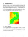
Topographic Information File ................................................................................... 6-3
DS-International, LLC
v
EFDC_Explorer
6.3
EFDC.INP Template File ......................................................................................... 6-3
6.4
Elevation Options .................................................................................................... 6-4
6.5
Grid Type................................................................................................................. 6-4
6.5.1.
Cartesian Grid.................................................................................................. 6-4
6.5.1.1 Uniform Grid................................................................................................. 6-5
6.5.1.2 Expanding Grid ............................................................................................ 6-5
6.5.2.
Riverine Curvilinear Grid .................................................................................. 6-7
6.5.3.
Import Grid ....................................................................................................... 6-9
7
ViewPlan ......................................................................................................................... 7-1
7.1
Simulation Results Loading ..................................................................................... 7-3
7.2
Introduction.............................................................................................................. 7-4
7.2.1.
Mouse Functions.............................................................................................. 7-5
7.2.1.1 Repositioning Legend & Other Objects ........................................................ 7-5
7.2.1.2 Cell Information ............................................................................................ 7-5
7.2.1.3 Right Mouse Click ........................................................................................ 7-6
7.2.2.
Keystroke Functions ........................................................................................ 7-7
7.2.3.
Toolbar Summary ............................................................................................ 7-9
7.2.3.1 Export EMF Files ....................................................................................... 7-10
7.2.3.2 Export Tecplot Files ................................................................................... 7-10
7.2.3.3 Create New EFDC Model ........................................................................... 7-11
7.2.3.4 Polyline/Polygon Creation Tool .................................................................. 7-11
7.2.3.5 View Calibration Data ................................................................................. 7-12
7.2.4.
Navigating the View ....................................................................................... 7-13
7.2.5.
Reporting Units .............................................................................................. 7-13
7.2.6.
Second Layer................................................................................................. 7-13
7.3
ViewPlan Display Options ...................................................................................... 7-14
7.4
General Pre-Processing Functions ........................................................................ 7-17
7.4.1.
Single Cell Edits ............................................................................................. 7-17
7.4.2.
Multiple Cell Edits .......................................................................................... 7-18
7.4.3.
Cell to Cell Copy/Assign................................................................................. 7-18
7.4.4.
Data Field Smoothing .................................................................................... 7-19
7.5
General Post-Processing Functions....................................................................... 7-19
7.5.1.
Time Series.................................................................................................... 7-19
7.5.2.
General Statistics ........................................................................................... 7-19
7.5.3.
Animation of Results ...................................................................................... 7-20
7.6
ViewPlan Main Viewing Options ............................................................................ 7-20
7.6.1.
Cell Indexes ................................................................................................... 7-20
7.6.2.
Cell Map ........................................................................................................ 7-21
7.6.3.
Bottom Elev ................................................................................................... 7-22
7.6.3.1 Bathymetry Comparison ............................................................................. 7-22
7.6.4.
Water Levels .................................................................................................. 7-22
7.6.5.
Boundary C's ................................................................................................. 7-24
7.6.6.
Fixed Params................................................................................................. 7-24
7.6.7.
Model Metrics ................................................................................................ 7-25
7.6.8.
Velocities ....................................................................................................... 7-26
7.6.8.1 Profile Tool ................................................................................................. 7-26
7.6.8.2 Water Flux Tool.......................................................................................... 7-26
7.6.9.
Sediment Bed ................................................................................................ 7-28
7.6.9.1 Toxics ........................................................................................................ 7-29
7.6.9.2 Bed Processes ........................................................................................... 7-29
DS-International, LLC
vi
EFDC_Explorer
7.6.10. Bed Heat ........................................................................................................ 7-29
7.6.11. Water Column ................................................................................................ 7-30
7.6.11.1
Longitudinal Profile ................................................................................. 7-30
7.6.11.2
Water Quality ......................................................................................... 7-32
7.6.11.3
Irradiance ............................................................................................... 7-32
7.6.11.4
Habitat Analysis ..................................................................................... 7-33
7.6.11.5
Volumetric Analysis ................................................................................ 7-34
7.6.12. Sediment Diagenesis/Specified Fluxes .......................................................... 7-36
7.6.12.1
Sediment Diagenesis ............................................................................. 7-36
7.6.12.2
Sediment Flux ........................................................................................ 7-37
7.6.13. Vegetation Map .............................................................................................. 7-37
7.6.14. Internal Variables (EFDC_DS Only) ............................................................... 7-37
7.6.15. ModChannel .................................................................................................. 7-38
7.6.16. Wave Parameters .......................................................................................... 7-38
8
ViewProfile ...................................................................................................................... 8-1
8.1
Slice/Profile Selection .............................................................................................. 8-1
8.2
Toolbar Summary .................................................................................................... 8-2
8.3
Primary Display Options .......................................................................................... 8-2
8.4
Function Keys .......................................................................................................... 8-4
9
Time Series Plotting Utility............................................................................................... 9-1
9.1
Analysis and Statistics ............................................................................................. 9-3
9.2
Series Options ......................................................................................................... 9-3
10
References .................................................................................................................... 10-1
Appendix A: EFDC Internal Array Visualization Instructions ................................................... A-1
Appendix B: Data Formats ..................................................................................................... B-1
DS-International, LLC
vii
EFDC_Explorer
List of Tables
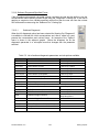
Table 1-1
Table 1-2
Table 3-1
Table 4-1
Table 7-1
Table 7-2
Table 7-3
Table 7-4
Table 7-5
Table 8-1
Table 9-1
EFDC_Explorer user interface conventions. ........................................................... 1-7
Operator descriptions. ............................................................................................ 1-8
Main toolbar summary of functions. ........................................................................ 3-2
Dye “decay” rate options. ..................................................................................... 4-25
Main Functions of ViewPlan ................................................................................... 7-1
ViewPlan keystroke function summary. .................................................................. 7-7
Summary of ViewPlan toolbar. ............................................................................... 7-9
Water quality parameter list available for display. ................................................. 7-35
List of sediment diagenesis parameters and sub-options available. ..................... 7-36
Summary of ViewProfile toolbar. ............................................................................ 8-3
Summary of Time Series Plotting Utility toolbar. ..................................................... 9-2
DS-International, LLC
viii
EFDC_Explorer
List of Figures
Figure 1-1 EFDC_Explorer Splash Screen ............................................................................. 1-1
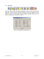
Figure 2-1 Main EFDC_Explorer form .................................................................................... 2-1
Figure 3-1 Main form toolbar .................................................................................................. 3-1
Figure 3-2 Project Open (Main Form)..................................................................................... 3-1
Figure 3-3 Select Directory: Open Operation ......................................................................... 3-3
Figure 3-4 Select Directory: Write Operation .......................................................................... 3-4
Figure 3-5 Printer Setup. ........................................................................................................ 3-5
Figure 3-6 EFDC_Explorer settings form................................................................................ 3-6
Figure 3-7 Julian to Gregorian Date conversion ..................................................................... 3-7
Figure 3-8 Toolbar functions .................................................................................................. 3-8
Figure 3-9 Grid Tools functions ............................................................................................ 3-10
Figure 3-10 Example of the model run times. ....................................................................... 3-12
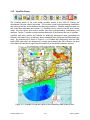
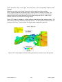
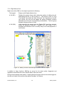
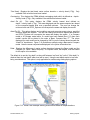
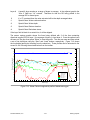
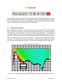
Figure 3-11 Example of ViewPlan output for the Perdido Bay water quality model. .............. 3-13
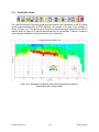
Figure 3-12 Example of ViewProfile output showing dissolved oxygen for Perdido Bay water
quality model. ................................................................................................................ 3-14
Figure 4-1 Tab: Model Title, Timing and Output. .................................................................... 4-1
Figure 4-2 Runtime, Output and Title. .................................................................................... 4-2
Figure 4-3 Tab: GVC. ............................................................................................................. 4-4
Figure 4-4 Tab: Grid, numerical solution and miscellaneous options. ..................................... 4-5
Figure 4-5 Mask Editing Tool. ................................................................................................ 4-6
Figure 4-6 Tab: Computational Options.................................................................................. 4-7
Figure 4-7 Tab: Hydrodynamics. ........................................................................................... 4-8
Figure 4-8 Eddy Viscosities & Diffusivities. ............................................................................. 4-9
Figure 4-9 Turbulent Intensities. ............................................................................................. 4-9
Figure 4-10 Wave Turbulence Tab: Internally Generated Wind Waves ................................ 4-10
Figure 4-11 Wave Turbulence Tab: Wave Options ............................................................... 4-11
Figure 4-12 Wave generated turbulence, import data form................................................... 4-11
Figure 4-13 Wave parameters: Radiation shear stress XX component. ............................... 4-12
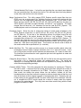
Figure 4-14 Vegetation class parameters. ............................................................................ 4-13
Figure 4-15 Cell property assignments: Vegetation map with IDs......................................... 4-14
Figure 4-16 Example vegetation map assignment. ............................................................... 4-14
Figure 4-17 Tab: Sed/Tox/Others. ........................................................................................ 4-15
Figure 4-18 Sediment Transport – General .......................................................................... 4-16
Figure 4-19 Sediment Transport – Cohesives. ..................................................................... 4-16
Figure 4-20 Sediment Transport – Non-Cohesives Suspended............................................ 4-17
Figure 4-21 Sediment Transport – Non-Cohesives Bedload................................................. 4-18
Figure 4-22 Sediment Transport – Bed and Consolidation. .................................................. 4-19
Figure 4-23 Sediment Transport – Initial Conditions. ............................................................ 4-20
Figure 4-24 Uniform sediment bed generation tool. .............................................................. 4-21
Figure 4-25 Sediment Bed Model: Cohesives Tab. .............................................................. 4-21
Figure 4-26 Tab: Sediment Bed Model: Initial Conditions Tab. .............................................. 4-22
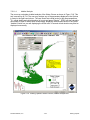
Figure 4-27 Example digital sediment model generated from sediment cores with grainsize.4-23
Figure 4-28 Toxic Transport Options. ................................................................................... 4-24
Figure 4-29 Atmospheric Parameters. .................................................................................. 4-26
Figure 4-30 Tracer generation tool. ...................................................................................... 4-27
Figure 4-31 Tab: Water Quality – General............................................................................ 4-28
Figure 4-32 Tab: Benth/Nutrients ......................................................................................... 4-28
Figure 4-33 Sediment nutrient flux – Sediment Diagenesis Options and Parameters. .......... 4-29
DS-International, LLC
ix
EFDC_Explorer
Figure 4-34 Sediment Diagenesis: Diagenesis – Options. .................................................... 4-29
Figure 4-35 Sediment Diagenesis: setting the initial conditions. ........................................... 4-30
Figure 4-36 Sediment Diagenesis: Diagenesis kinetic zones. .............................................. 4-31
Figure 4-37 Tab: Algae/ WQ IC’s. ........................................................................................ 4-31
Figure 4-38 Algal Dynamics parameter form. ....................................................................... 4-32
Figure 4-39 Tab: Water Quality Boundary Conditions and Lagrangian Particle Tracking. ..... 4-33
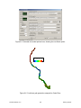
Figure 4-40 LPT Main Options tab. ...................................................................................... 4-35
Figure 4-41 LPT: Initial Position Seeding Utility. ................................................................... 4-36
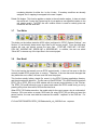
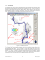
Figure 4-42 Harbor_U grid showing the masks, boundaries and initial particle locations. ..... 4-37
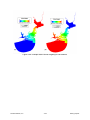
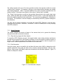
Figure 4-43 Harbor_U: Trajectories of 5 drifters over 1 day (no random walk). ..................... 4-38
Figure 4-44 Harbor_U: Trajectories of 5 drifters over 1 day (random walk). ......................... 4-38
Figure 4-45 Tab: Initial “Conditions”. .................................................................................... 4-39
Figure 4-46 Apply Cell Properties via Polygons.................................................................... 4-39
Figure 4-47 Tab: Boundary Conditions ................................................................................. 4-41
Figure 4-48 Example WSER series weighting for two stations. ............................................ 4-43
Figure 4-49 Boundary Condition Definitions/Groups............................................................. 4-44
Figure 4-50 HSPF model results import utility. ..................................................................... 4-46
Figure 4-51 View loadings options form. .............................................................................. 4-48
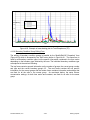
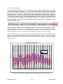
Figure 4-52 Example of mass loading plot for Total Phosphorus (TP). ................................. 4-49
Figure 4-53 Modify/Edit Boundary Condition Properties. ...................................................... 4-50
Figure 4-54 Boundary conditions time series editor. ............................................................. 4-53
Figure 4-55 ASCII data time series import form. ................................................................... 4-56
Figure 4-56 Time series keystroke function help message. .................................................. 4-57
Figure 5-1 Tab: Hydrodynamics. ............................................................................................ 5-2
Figure 5-2 Example grid profile plot........................................................................................ 5-2
Figure 5-3 Example water surface elevation profile with bathymetry. ..................................... 5-3
Figure 5-4 Tab: Miscellaneous Series. ................................................................................... 5-4
Figure 5-5 Example of sediment column consolidation: (a) Initial conditions (b) End of Day 1 5-4
Figure 5-6 Example “Bed Top Profile” for water column and sediment bed. ........................... 5-5
Figure 5-7 Mass Balance Tool Options Form. ........................................................................ 5-6
Figure 5-8 Tab: Comparison Data. ......................................................................................... 5-6
Figure 5-9 Load a comparison EFDC model .......................................................................... 5-7
Figure 5-10 Loading measured 2D calibration data. ............................................................... 5-8
Figure 5-11 Example 2D velocity data comparison. ................................................................ 5-9
Figure 5-12 Tab: Calibration Plots ........................................................................................ 5-10
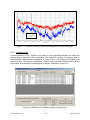
Figure 5-13 Example time series calibration statistics report. ............................................... 5-12
Figure 5-14 Time series calibration EFDC cell and data linkage definitions. ......................... 5-13
Figure 5-15 Available calibration parameter codes. .............................................................. 5-14
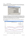
Figure 5-16 Example model-data time series comparison for water levels. .......................... 5-15
Figure 5-17 Example model-data time series comparison for dissolved oxygen. .................. 5-16
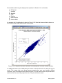
Figure 5-18 Calibration tool: Model vs Data Correlation Plots. ............................................. 5-16
Figure 5-19 Example model data Correlation Plots comparison for water surface elevation. 5-17
Figure 5-20 Vertical profile calibration EFDC cell and data linkage definitions...................... 5-18
Figure 5-21 Example model-data vertical profile plot for salinity. .......................................... 5-19
Figure 6-1 Generate new model options form, with expanding Cartesian option. ................... 6-1
Figure 6-2 Example digital topographic data .......................................................................... 6-3
Figure 6-3 Cartesian gridding: Expanding & rotated grid. ....................................................... 6-5
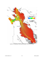
Figure 6-4 Expanding Cartesian grid example of San Francisco Bay. .................................... 6-6
Figure 6-5 Generate new model options form, showing the curvilinear option. ....................... 6-8
Figure 6-6 Curvilinear grid generation example for Cedar River ............................................. 6-8
Figure 6-7 Grid generation: Import Delft’s RGFGrid. .............................................................. 6-9
DS-International, LLC
x
EFDC_Explorer
Figure 7-1 Model results loading options. ............................................................................... 7-3
Figure 7-2 ViewPlan main form. ............................................................................................. 7-4
Figure 7-3 Cell Information example ...................................................................................... 7-5
Figure 7-4 Modify Cell form with bed layer-sediment mass sub-option. .................................. 7-6
Figure 7-5 ViewPlan Toolbar. ................................................................................................. 7-9
Figure 7-6 Tecplot export timing options. ............................................................................. 7-11
Figure 7-7 ViewPlan Display Options: General Options. ...................................................... 7-14
Figure 7-8 ViewPlan Display Options: Velocity/Boundary Conditions. .................................. 7-15
Figure 7-9 ViewPlan Display Options: Annotations. ............................................................. 7-16
Figure 7-10 ViewPlan Display Options: Particle Tracks. ....................................................... 7-17
Figure 7-11 Example Cell Map. ............................................................................................ 7-21
Figure 7-12 Water Level example showing Areal Extents based on depth-durations. .......... 7-23
Figure 7-13 Water flux tool control options. .......................................................................... 7-26
Figure 7-14 Water Flux tool example results using Dominant Flow. ..................................... 7-27
Figure 7-15 Viewing Options: Sediment Bed with Cell Editing .............................................. 7-28
Figure 7-16 Water Column longitudinal profile of dissolved oxygen. ..................................... 7-31
Figure 7-17 Viewing Options: Water Column, % Irradiance Tool. ......................................... 7-32
Figure 7-18 Viewing Options: Water Column, Habitat Analysis tool. ..................................... 7-33
Figure 7-19 Viewing Options, Volumetric Analysis Tool. ...................................................... 7-34
Figure 7-20 Viewing Options: Volumetric Analysis Time Series. .......................................... 7-34
Figure 7-21 Add/Edit Channel Modifier option form .............................................................. 7-38
Figure 8-1 ViewProfile example showing salinity at one snapshot in time during a tidal cycle 8-1
Figure 8-2 Profile display options. .......................................................................................... 8-2
Figure 8-3 ViewProfile keystroke functions. ........................................................................... 8-4
Figure 9-1 Time Series Plotting (TSP) utility. .......................................................................... 9-1
Figure 9-2 TSP Line Options and Controls form. .................................................................... 9-4
Figure 9-3 TSP Utility standard value axis options form. ........................................................ 9-5
Figure 9-4 TSP Utility date axis options form.......................................................................... 9-5
DS-International, LLC
xi
EFDC_Explorer
1 Introduction
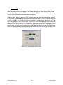
EFDC_Explorer (Figure 1-1) is a Microsoft Windows™ based pre-processor and postprocessor for the three-dimensional (3D) hydrodynamic model, Environmental Fluid
Dynamics Code (EFDC), initially developed at the Virginia Institute of Marine Science
(Hamrick, 1992 & 1996). The US Environmental Protection Agency (EPA) has continued to
support its development. The EFDC code is public domain and part of a family of models
recommended
by
EPA
for
environmental
and
regulatory
applications
(www.epa.gov/ceampubl/swater/efdc).
Figure 1-1 EFDC_Explorer Splash Screen.
EFDC is a general-purpose model for simulating three-dimensional (3-D) flow, transport, and
biogeochemical processes in surface water systems including: rivers, lakes, estuaries,
reservoirs, wetlands, and near-shore to shelf-scale coastal regions. EFDC is capable of
simulating cohesive and non-cohesive sediment transport, near-field and far-field plume
discharge from multiple sources, and the transport and fate of toxic contaminants in the
water and sediment phases. A dissolved oxygen/nutrient process (i.e. eutrophication) submodel (HEM-3D) was added later (Park, et al., 2000). Special enhancements to the
hydrodynamics of the code now include vegetation resistance, drying and wetting, hydraulic
structure representation, wave-current boundary layer interaction and wave-induced
currents. The EFDC code has been extensively tested and the code is currently used by
university, government, and engineering and environmental consulting organizations.
The EFDC model has been released in the past in various forms and versions. This user’s
manual focuses on only two versions, the EPA Version 1.01 (EFDC_EPA) September 2007
(Tetra Tech, 2007a, 2007b) and the EFDC_DS Version 2009_11_01. The EFDC_EPA
version has an implementation of the Generalized Vertical Coordinate (GVC) system (Stacey
et al., 1995; Adcroft and Campin, 2004, TetraTech, 2006) that is supported in the current
version of EFDC_Explorer.
This user’s manual provides guidance in the use EFDC_Explorer. This manual is NOT a
user’s manual for EFDC. It is assumed that the user is familiar with the types of data and
information required by EFDC. EFDC_Explorer is a tool to assist qualified engineers and
scientists in the development, testing, calibration and interpretation/analysis of the model.
DS-International, LLC
1-1
EFDC_Explorer
1.1
EFDC_Explorer Capabilities
The following lists provide a summary of the major features of EFDC_Explorer. The lists are
grouped into three primary categories based on the general use of each feature. The first
group contains general purpose features while the other two groups summarize the major
pre- and post-processing features.
It is recognized that many more options and features could be added to EFDC_Explorer. It
is anticipated that many new features will be added as resources are available.
General
Graphical interface to most of the commonly used EFDC features.
Graphical interface for EFDC (Sigma & GVC versions) sub-models:
o Hydrodynamics
o Density dependent flow state variables: Salinity/Temperature
o Tracer
o Sediment Transport
o Toxics
o Water Quality with Sediment Diagenesis
Extensive visualization and point and click inquiries of input and output data.
Extensive use of popup tips to help the user select the proper inputs.
Extensive error and range checking for user inputs.
Many functions work with Calendar date and/or Julian dates
Binary file access method to allow the access to files > 4.2GB.
Any number of snapshots that can be written by EFDC and managed/used by
EFDC_Explorer.
Output Plots and Tables in either Metric or English units.
Continuing support and development of the utility.
Pre-Processor-General
Pre-Processor for the EFDC 2D-3D Version.
Import many previous versions of the main control file (i.e. EFDC.INP).
Courant # and Courant-Fredrick-Levy calculator tools.
Run logging.
Pre-Processor-Model Generation
Build Cartesian or simple Curvilinear models.
Cartesian models can use expanding grid spacing and grid rotations.
Easily increase or decrease vertical layering.
Import complex Curvilinear models generated by third party utilities:
o Delft RGFGrid formatted file (i.e. GRD file) ,
o Grid95,
o SEAGrid, and
o Any generic cell based nodal coordinate file.
Import grids from different hydrodynamic models:
o CH3D-WES,
o CH3D-IMS,
o ECOMSED, and
o Prior versions of EFDC.
Import grids with multiple sub-domains
DS-International, LLC
1-2
EFDC_Explorer
Pre-Processor-General Grid Tools
Grid Orthogonality statistics and plots.
Export any EFDC model grid as an RGFGrid formatted GRD file.
Export the model domain outline as a XY file (P2D format).
Export the model cells as a XY file (P2D format).
Transpose and/or flip the I and J indexes.
Clean and repair any DX/DY and cell angle problems using a repair utility.
Pre-Processor-Initial Conditions
Easy and fast plan views of the model domain with model option specific viewing
options.
Develop/Edit bathymetry from Digital Terrain Models (DTM’s) or irregularly spaced
elevation data.
Build/Edit sediment beds with toxics.
Set and edit cell properties by “point & click” on the model grid.
User defined polygon cell selections for editing.
Use simple operators to edit one or any number of cells.
View/Set Vegetation mapping (if used).
View/Set Groundwater mapping (if used).
Refine grid manually by activating/deactivating cells from the cell map.
Rapid setting of the initial conditions water surface or depths.
Use of 3D polylines to assist in setting initial conditions.
Create/Read a compact binary “archive” file for a model run.
Assign initial conditions using spatially varying vertical measured/estimated profiles.
View/Assign/Edit roughness field.
View Courant #/CFL map.
View/Assign/Edit "Channel Modifier" information/configuration (if used).
Set particle seeding and Lagrangian Particle Tracking control options.
Pre-Processor-Boundary Conditions
Define/Edit/Plot flow, hydraulic structure, open and withdrawal/return type boundary
condition groups.
Define harmonic tides
Set and edit boundary conditions by “point & click” on the model grid.
Boundary conditions time series intelligent editor and one-button plotting.
Use familiar names to identify and label boundary cells and input time series.
Label boundary groups on 2D maps and/or export group labels to a file for more
control over labeling of maps in EFDC_Explorer or GIS applications.
HSPF model boundary condition interface to quickly import HSPF results to EFDC.
Generate spatially interpolated time series for open boundary conditions.
Use concentrations instead of mass loading (HEM3D default) for the water quality
flow type BC groups.
Pre-Processor-Mass Balance/Boundary Loadings
Compute mass balance of various model constituents with plotting and tabular output
of time series.
Plot the boundary condition loadings for various model constituents or some derived
parameters like Total Phosphorus, Total Nitrogen or Total Carbon.
Compute average and cumulative loadings using the “Averaging” and “Integration”
features of the time series plotting utility.
DS-International, LLC
1-3
EFDC_Explorer
Generate mass loading summary tables for each simulated parameter.
Pre-Processor-Utilities
Tracer configuration utility.
A bitmap geo-referencing tool.
Perform QA checks on input data prior to model runs.
Merge multiple continuation runs into single data sets
Create new model runs from any saved results from previous runs.
Unix to Windows CR/LF conversion.
Post-Processor-General
Post-Processor for the 3D sigma stretch and GVC versions of EFDC.
Calendar day/Julian date labeling of plots and animations.
EFDC output file management utility for resampling (i.e. reducing snapshot
frequency) or merging continuation runs into a single output file.
High Frequency Snapshot capability to insert high resolution results snapshots into
the standard EFDC snapshot frequency.
Optionally plot the color ramp in grey scale (for publications).
Toggle on/off the display of titles on plots (for reports and publications).
DS-International, LLC
1-4
EFDC_Explorer
Post-Processor-ViewPlan (2D Plan)
View/label cell maps.
Quickly animate many of the results to the screen or an AVI file.
Export results to the commercial graphics package TECPlot®.
Compute model results statistics for current view or by polygon.
Overlay the model with line drawings and labels.
Display one or more georeferenced bitmaps as a background to the model grid.
o Several views allow for transparent grid cells to view the background and
model results.
Display a “Timing Frame” to temporally reference results to a boundary condition,
like:
o Tide series
o Inflows/Outflows
o Winds
Display spatial scales in various units.
Generate a new model from the output of an existing model for any selected time,
View water surface/depth maps, animations and time series.
o Transparent Cells for water depths/elevations and other water column results.
o Flood Inundation Mapping
o Compute/Display areal extents based on specified a minimum depth and
duration.
o Compute/Display areal extents based on a Depth*Velocity Flood Hazard
Factor.
o Compare up to 3 models on the same plot showing Areal Extents.
o Energy Mapping
Compute/Display total head (WS Elevation + v2/2g).
Compute FEMA Overtopping parameter (depth + v2).
View Sediment/Bottom results for any time output or animation, (by layer or
averaged/totaled over the number of sediment layers):
o Bottom topography elevations,
o Bottom scour/deposition,
o Bottom grain size distributions,
o Bottom sediment mass distributions (by layer or totaled over the total number
of layers (i.e. KB),
o Bottom sediment mass fractions (by layer or averaged over KB),
o Bottom sediment porosity (by layer or averaged over KB),
o Bed surface shear stress.
View Water Column results for any time output or animation, (by layer or
averaged/totaled over the number of water column layers):
o Salinity,
o Temperature,
o Dye or a computed Age of Water (EFDC_DS Only),
o Toxics,
Totals
DOC Complexed
Dissolved, and
POC Adsorbed.
o Sediments (by class or totaled).
o Water quality parameters
22 EFDC modeled constituents
Derived parameters like Chl-a, algal growth limiters, and TSI’s.
o Anoxic volumes (User specified DO cutoff)
o Light penetration (Secchi Depth, Extinction Coefficients, % Irradiance).
DS-International, LLC
1-5
EFDC_Explorer
View boundary conditions map and view boundary condition time series.
o View profiles of sediment bed and water column properties with time.
o Store and quickly display time series calibration comparisons.
o Compare velocity data to other model runs or field data (e.g. ADCP)
o Compare model results from two different models to each other.
View Sediment Diagenesis concentrations and nutrient fluxes
o View by class or total concentrations of PON, POP & POC
o View concentrations by diagenesis layer or totals
o View nutrient fluxes
Model Metrics
o Grid Orthogonality map & statistics,
o Cell angle maps,
o Courant Number,
o Courant-Friedrichs-Levy (CFL) time step limits,
o Froude Number,
o Densimetric Froude Number,
o Celerity, and
o Richardson Number.
View Longitudinal Profile plots
o Generate longitudinal plots of water column and bottom sediments results.
o User specified layer averaging (e.g. "1-3” will average the bottom three
layers).
o Water column or bottom sediment data can be overlaid with bottom
topography and/or water surface elevation/depth results and/or bed shear.
Overlay plan view plots with the following Calibration Data/Information:
o Station ID,
o Date/Time coordinated data values,
o Date/Time coordinated data residuals, and
o Data values and residuals can use the same depth averaging or specified
layer options specified for the model results.
View plotting and animation of Lagrangian Particle Tracking.
o Added the ability to export one or more particle tracks to ASCII files for
linkage to 3rd party applications.
Post-Processor- Vertical Profiles
View 2D vertical section plots along any I or J index or user defined polyline.
For any vertical section view/animate:
o Velocities,
o Salinity,
o Temperature,
o Dye or a computed Age of Water (EFDC_DS Only),
o Toxics,
o Sediments, and
o Water quality parameters.
Post-Processor-Miscellaneous
Water flux calculator by layer or totaled for all layers.
Sediment mass balance/sediment mass loadings.
Post-Processor-Calibration Comparisons
Time series comparisons for water column data of measured to modeled data for any
layer, depth averaged and/or Min-Avg-Max model results.
Vertical profile comparisons.
DS-International, LLC
1-6
EFDC_Explorer
Produce report ready graphics.
Calibration statistics using RMS Error, Average Error, Absolute Error, Relative Error
and/or Nash-Sutcliffe Efficiency Coefficient.
Automatic generation of the calibration plots and correlation plots with calibration
statistics.
Comparison of model results between multiple model runs.
1.2
Recent Enhancements to EFDC_Explorer Capabilities
Addition of dye modeling capability
Water Quality Boundary Conditions can now be loaded as Concentrations rather than
just Mass Loadings
Addition of Withdrawal/Return Boundary Condition
Ability to compare Bathymetry between models
Extracting Time Series is now simpler and easier
Time Series Plots now include box and whisker plots as well as great control over
display of individual lines
Ability to created Correlation Plots for data versus model comparisons
Ability to internally compute bed shear stress due to Wind Waves
Addition of Lagrangian Particle Transport (LPT) sub-model.
1.3
Conventions
1.3.1. Windows Interface
While the general use of EFDC_Explorer is fairly standard with respect to a user interface for
the Windows® operating system, some basic conventions will be explained here that should
help the user.
Table 1-1 EFDC_Explorer user interface conventions.
A black box with green text provide information only, it cannot be edited from that
location. The information/data may be modified elsewhere.
A while box with black text is the primary data/text input interface.
A radial button indicates a range of options. Only one can be selected for each
operation requested.
The “Browse” button is used extensively in the program to allow the user the ability to
navigate to the requested/desired file(s) rather than typing in the adjacent text box.
The user will notice several “grayed out” or disabled features in EFDC_Explorer. This
indicates that a particular feature is not available for the currently applied version of EFDC or
unavailable based on the user selected options. The “grayed out” options are not available
to the user.
DS-International, LLC
1-7
EFDC_Explorer
1.3.2. Message Boxes and the Clipboard
During the use of EFDC_Explorer various informational message boxes will be displayed,
presenting the results of some calculation or other message. Most of these messages are
also placed into the Windows clipboard for ease of transferring the information to some other
applications. The data placed onto the clipboard are generally tab delimited.
1.3.3. Tooltips
When the cursor is passed over a button or field EFDC_Explorer will often show a tooltip that
will help to explain the function of that button.
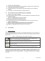
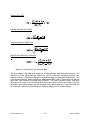
1.3.4. Operators
At several places in EFDC_Explorer the user has the option of entering a value to replace
the current value of some input parameter (e.g., bottom elevation) or to use an “operator”.
The latter is a simple mathematical function that will be applied to the current value of the
parameter. A field that allows “operators” recognizes the inputs described in Table 1-2.
Operators must be followed by a space then the value, unless it is a simple replacement
value.
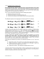
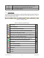
Table 1-2 Operator descriptions.
Input
A Number
+ Number
- Number
* Number
/ Number
Current
Value
300
300
300
300
300
Description
Replacement value
Additive Operation
Subtraction Operation
Multiplication Operation
Division Operation
Example
Input
“Operator”
310
+1
- 20
* 1.1
/ 1.1
Result
310
301
280
330
272.73
1.3.5. Units
EFDC uses the metric system to define the space and concentration variables. Meters are
used for all of the length related parameters and g/m 3 are used for concentrations, with the
exception of salinity (kg/m3) and toxics. For toxics, the units must be consistent between
concentrations and the water column and sediment bed sorption parameters. Generally,
these are in mg/m3 or g/m3.
The internal EFDC time units are in seconds. For EFDC, most of the input files can use any
units along with a conversion factor to change the input units to seconds. EFDC_Explorer
has fixed the user input units to days. All of the timing input should be in days and
EFDC_Explorer generates the necessary conversion factors to seconds.
DS-International, LLC
1-8
EFDC_Explorer
1.4
Terms & Abbreviations
The following is a description of common terms and abbreviations used in this report:
LMC
“Left Mouse Click”. On a standard mouse this refers to the left side button. Some
Windows configurations can reverse the function of the left and right mouse buttons.
RMC “Right Mouse Click”. On a standard mouse this refers to the right side button.
Ctrl
The “Control” key on the keyboard.
Alt
The “ALT” key on the Keyboard.
DS-International, LLC
1-9
EFDC_Explorer
2 Installation & Startup
2.1
Installation
1) If you received EFDC_Explorer in a zip file (EFDC_Explorer.ZIP), unzip the zip file into a
temporary directory on your hard drive. To simplify the cleanup of files later it is
recommended that the temporary directory be empty before unzipping.
2) You may either a) Select File|Run from the Program Manager or File Manager and run
the EFDC_Explorer Install program (SETUP.EXE), or b) use Explorer to display the
directory files in the directory you unzipped the files to and then double click the file
SETUP.EXE
3) Choose the directory and install EFDC_Explorer.
4) If you used a temporary directory you should delete the files that were unzipped. Keep a
copy of the zip file in case you need to install the program again.
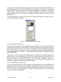
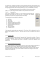
5) For Vista™ users, you may need to change the EFDC_Explorer5.exe to “Run as
Administrator” before you can use EFDC_Explorer to run models.
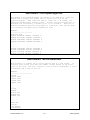
Figure 2-1 Main EFDC_Explorer form.
DS-International, LLC.
2-1
EFDC_Explorer
2.2
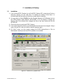
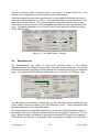
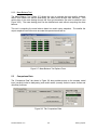
General Program Operation
Upon starting EFDC_Explorer the user will be presented with the form shown in Figure 2-1.
This form is basically divided into three parts. At the top of the form, the main Toolbar is shown
providing quick access to many of the primary EFDC_Explorer features and actions. The main
form is then divided into two primary sections. The upper section represents the pre-processor
functions and the lower section provides access to some of the post processor functions. The
operation and further instructions for each of these groupings will be described in the following
sections.
2.3
EFDC_Explorer Files
The main control file for every EFDC application is the EFDC.INP file. EFDC.INP is an ASCII
file structured into card groups that generally have the same basic objective, e.g. card group 8
(C8) contains the settings for the run time but it also contains other miscellaneous parameters.
This file contains almost all of the computational options and data settings.
The EFDC model uses fixed file names (e.g. DXDY.INP) based on the type of information each
file contains. The files that are required for a model application vary based on the
computational and grid options selected. For example, if the ISVEG flag (C5) is >0 then the
VEGE.INP file, which contains vegetation information to compute vegetation based flow
resistance, must be supplied. EFDC_Explorer reads and writes these same files and reduces
the need for the user to remember exactly which file and/or which card group has what flag or
setting.
EFDC_Explorer requires additional information and data to perform its pre-processing and
visualizations. When saving an existing or new project, EFDC_Explorer automatically
generates these files based on the project’s settings. The following provides a list of
EFDC_Explorer specific files and their functions:
EFDC.DS
This is the main EFDC_Explorer project file. This file contains
much of the labeling, formatting, boundary condition, and modeldata linkage information. This file is REQUIRED for
EFDC_Explorer to correctly manage boundary groups
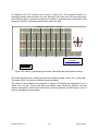
CORNERS.INP
This file contains the corner coordinates for each cell.
EFDC_Explorer computes these using the cell center coordinates,
DX, DY and cell rotation. It then matches the cell corners and
builds the nodal list. By default, EFDC_Explorer displays the 2D
plan view cells using these corner coordinates. However, the user
can choose to view the rectangular cells if desired.
EFDC_LOG.DS
This file contains the run log that is displayed in the main
EFDC_Explorer form. This file is ASCII and can be viewed with
any ASCII editor.
CalForm_TS.DS
This file contains formatting and labeling information for the time
series calibration plots.
CalForm_VP.DS
This file contains formatting and labeling information for the
vertical profile calibration plots.
DS-International, LLC.
2-2
EFDC_Explorer
In order for EFDC_Explorer to post-process the data the following files must be generated by
EFDC:
EE_WS.OUT
Required. This file contains the water depths.
EE_VEL.OUT
Recommended. This file contains the 3D velocity field.
EE_WC.OUT
This file contains the water column results as well as the
information for the top layer of the sediment bed.
EE_BED.OUT
This file contains the sediment bed data for each layer, including
the toxics associated with each layer.
EE_ARRAYS.OUT
This is an optional file that the EEXPOUT subroutine in EFDC
optionally generates. This file contains snapshots of almost any
internal EFDC array desired. EFDC_Explorer automatically loads
this file and provides visualization, if it exists. (See Appendix A for
more details).
EE_WQ.OUT
This file contains the water column results for water quality
constituents simulated.
EE_SD.OUT
This file contains the sediment diagenesis results if the full
sediment diagenesis option is turned on.
DS-International, LLC.
2-3
EFDC_Explorer
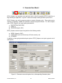
3 EFDC_Explorer Primary Toolbar
Upon starting EFDC_Explorer the user will be presented with the form shown in Figure 2-1.
This form is basically divided into three parts. The middle section represents the pre-processor
functions and the lower section provides access to some of the post-processor functions.
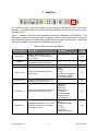
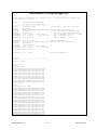
Another major section of EFDC_Explorer is the toolbar located at the top of the form (Figure
3-1). This provides access to the program configuration options and the main model viewing
functions. This section contains brief descriptions of several miscellaneous functions that are
available from the main toolbar of EFDC_Explorer.
Figure 3-1 Main form toolbar.
3.1
File Management
EFDC uses fixed file names for its input files; therefore each run/project should be stored in
separate directories. EFDC_Explorer operates in the same manner. EFDC_Explorer reads and
writes the files with the standard fixed file names to/from the specified subdirectory (called a
“project” by EFDC_Explorer).
Figure 3-2 shows the main file management toolbar and Browse buttons to access the opening
and/or saving of a project.
Figure 3-2 Project Open (Main Form).
DS-International, LLC.
3-1
EFDC_Explorer
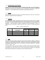
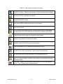
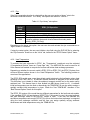
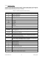
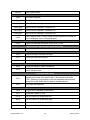
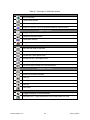
Table 3-1 Main toolbar summary of functions.
Exit EFDC_Explorer. Does not save project, only Pre-/Post-processor settings.
Generate an EFDC model using a template.
Open/Read an EFDC model.
Save current EFDC model into the same or new directory.
Setup current printer.
EFDC_Explorer configuration options, including where the EFDC executable
files are located, one for the EPA version and one for the EFDC_DS version.
Convert between Julian days and Gregorian calendar dates
Toolbox of miscellaneous features and utilities.
View/Edit main EFDC.INP file for the current project.
Various tools and utilities for analyzing and adjusting the grid.
Run EFDC using the current project. Does not save the project first.
Get runtime and other timing information for a completed model run.
ViewPlan. Display the model in plan view. This is used for some pre-processing
tasks (e.g. setting boundary conditions and modifying cell properties) and postprocessing results.
ViewProfile. Display the model profile view along an I or J or a user defined
section. This is used for post-processing results.
DS-International, LLC.
3-2
EFDC_Explorer
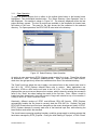
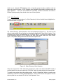
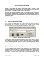
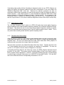
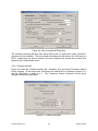
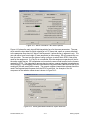
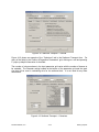
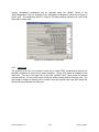
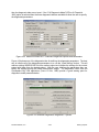
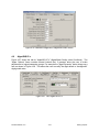
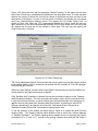
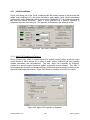
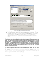
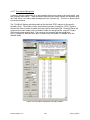
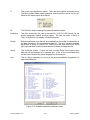
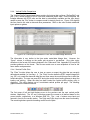
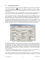
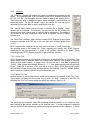
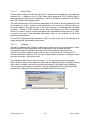
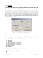
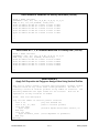
3.1.1. Open Operation
To open an existing project click on either on the toolbar folder button or the browse button
highlighted. They accomplish identical tasks. The “Select Directory: Open Operation” form is
then displayed. An example is shown in Figure 3-3. The directory displayed will be the last
project directory opened. The last 20 projects are available in the dropdown list located near
the bottom of the form. The panel on the right shows the files contained in the selected
directory. For Open operations, the EFDC.INP file must exist in the directory.
Figure 3-3 Select Directory: Open Operation.
An option to open a previously EFDC_Explorer saved archive file is given. These files all have
an extension of “efdc”, for example “CedarRiver.efdc”. When you select the “Open Archive”
check box, the right panel only shows the available archive files in the selected directory.
The “Scale” input box allows the user to apply a conversion factor to the centroid units used in
the LXLY file. EFDC_Explorer defaults these units to meters. Many applications use
kilometers, UTM’s or miles as the unit base in the LXLY file. For the model to be correctly
displayed the user must convert these units to meters, which is done by entering the conversion
factor in the “Scale” box when loading the model for the first time. Note: When a model is
loaded and then viewed and it looks like a bunch of large cells stacked on top of one another, it
is likely to be a LXLY units conversion issue.
Historically, different versions of EFDC used different CELL.INP formats. EFDC_Explorer
automatically handles the file format to correctly load the CELL.INP file. Similarly, the main
EFDC.INP file and other input files have changed over the recent development history of EFDC.
EFDC_Explorer attempts to correctly read most of the historical input files, while ensuring the
latest version works and is the standard.
The check boxes concerning resetting boundary condition groups apply to existing projects that
have been managed by EFDC_Explorer. During the initial loading of a project, or if the “Reset”
DS-International, LLC.
3-3
EFDC_Explorer
check box is selected, EFDC_Explorer tries to logically group boundary condition cells into
groups by type and location. EFDC_Explorer then manages the boundary conditions using this
group approach. If the user has modified the boundary conditions somehow and wants a
different logical grouping, they should select one of these options.
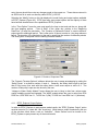
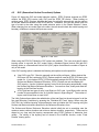
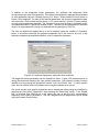
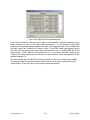
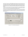
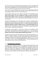
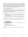
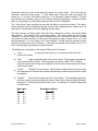
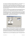
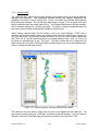
3.1.2. Write Operation
To save a currently opened project (i.e. Write Operation), click on the disk button highlighted on
the toolbar shown in Figure 3-2.
The “Select Directory: Write Operation” form will be displayed (Figure 3-4). The user has the
option to select which files are written by selecting the appropriate “Save Option” button. For a
complete save of all the input files select the “Full Write” option. If you have only made changes
to the formatting options in EFDC_Explorer and want those saved, select the “Save Profile”
option. The profile is always saved for the other save options also.
Figure 3-4 Select Directory: Write Operation.
If the user only has the “.efdc” archive file and wants to create a set of files that EFDC needs to
run that project, the user must select the “Full Write” option to create all the input files required.
To create a new project using the existing project, use the “Create New” button to create a new
subdirectory under the currently displayed directory. All the .INP files will be copied to the new
directory after the user selects OK on the “Write Operation” form.
DS-International, LLC.
3-4
EFDC_Explorer
Cross Platform Note
Many users may want to use EFDC on both a PC and a UNIX
based computer. When transferring the input files from the UNIX
machine to the PC, the carriage control MUST be reset to the
Windows/DOS carriage control.
EFDC_Explorer has the ability to convert non-Windows/DOS
carriage control to Windows/DOS, via the Toolbox.
Also, the user may use one of several ASCII editors that have
this capability as well.
If the user wishes to save in the EPA GVC Model format rather than EFDC_DS model format
this should be selected in the “GVC” tab of the “EFDC Information and Pre-processing” frame of
the main EFDC_Explorer form. This method allows quick reformatting of the EFDC.INP file for
the different models. Care must be exercised to ensure that all the parameters have the desired
values when switching models (see Section 4.2).
3.2
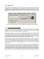
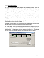
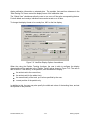
Printer Setup
The current default printer is automatically used by EFDC_Explorer. Figure 3-5 shows an
example printer setup form that appears when the highlighted toolbar button is pushed. If no
printers are available during the startup of EFDC_Explorer, it will display a warning but will
continue. Besides being used for printing, the settings from this form also impact certain
exported graphics. The primary setting used is the portrait versus landscape option to set page
orientation.
Figure 3-5 Printer Setup.
DS-International, LLC.
3-5
EFDC_Explorer
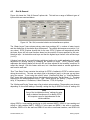
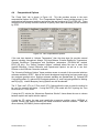
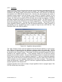
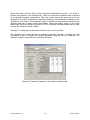
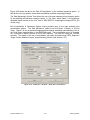
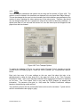
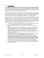
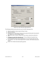
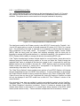
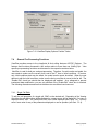
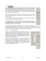
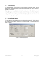
3.3
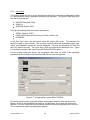
EFDC_Explorer Settings
This toolbar button allows the user to specify some installation specific parameters, like the
location of the EFDC executable to use, as well as project specific settings like default
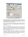
precisions. Figure 3-6 shows the settings form.
The precision settings are for setting the output/display precisions for the indicated data types.
The default settings shown are appropriate for most applications. However, for special cases
(e.g. flume studies or other types of research applications) the user will likely have to make
adjustments to the defaults. This information is stored in the project specific EFDC.DS file. The
default settings for EFDC_Explorer are saved in the EFDC_EXPLORER.INI file that is located in
the same directory as the EFDC_Explorer executable.
Many installation/machine specific default EFDC_Explorer settings are saved in the
EFDC_Explorer.INI file. This is an editable ASCII file, though care should be exercised to not
corrupt the file. The file structure follows the Windows standard INI file using groups and tags.
The project specific settings for information/data that the EFDC model does not use (i.e. labels,
plot formatting, etc) are saved in the EFDC.DS file that is located in the project directory. If the
user wants to maintain a complete data set (either with all the ASCII .INP files or the binary
archive file) the user must also save the EFDC.DS file. This also applies when the user is
sending the model to another person. The EFDC.DS file is also an ASCII file that can be edited
with any ASCII editor.
Figure 3-6 EFDC_Explorer settings form.
DS-International, LLC.
3-6
EFDC_Explorer
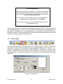
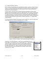
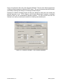
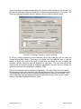
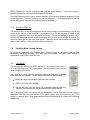
3.4
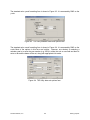
Julian to Gregorian Calendar Converter
This toolbar button brings up a calendar conversion function (Figure 3-7) that allows the number
of days to be calculated from the time of a Base Date to the time of a specified Gregorian
calendar date. If the Gregorian date entered is before the Base Date a negative number of
Julian days in given. This tool can also be used to determine a Gregorian Date, given any
number of days before (<0) or after (>0) a given Base Date.
The default Base Date is the Project’s Base Date. However the user can change the Base Date
in this utility without impacting the Project’s Base Date.
Figure 3-7 Julian to Gregorian Date conversion.
DS-International, LLC.
3-7
EFDC_Explorer
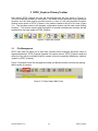
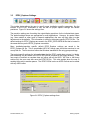
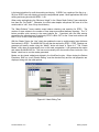
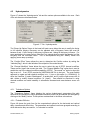
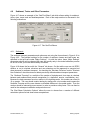
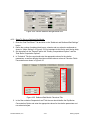
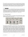
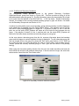
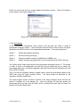
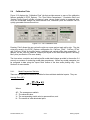
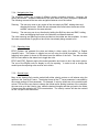
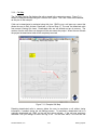
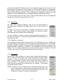
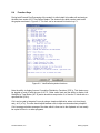
3.5
Toolbag: General Utilities
The Toolbar function provides access to a range of general utilities that support the modeling
process but may not be directly related to the EFDC model. Figure 3-8 shows a screen capture
of the current functions available under the Toolbag. The following list provides a summary of
these functions.
Figure 3-8 Toolbar functions.
Bitmap Georeferencing: This utility can be used to create or edit the configuration file that
EFDC_Explorer uses to provide bitmap images and maps as a background for the
display of models in ViewPlan. To use bitmaps you must first create a “geo” file. This is
an ASCII file with the extension “geo” that contains the pixel and project coordinate
information. It is very similar to MapInfo’s TAB format. One “geo” file can reference
multiple bitmaps to build mosaics, if needed. When this function is selected a form is
displayed with the bitmap filenames and coordinate information. Any changes must be
saved into the same or new “geo” file for later use in ViewPlan.
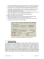
Unix -> Windows CRLF Conversion: This utility scans a specified directory and determines if
any of the files contained in the directory do not use the Windows CRLF standard. The
user then has the option of automatically converting all non-Windows CRLF files to the
Windows standard. EFDC_Explorer uses the Windows CRLF convention, so files
created or edited on a Unix platform need to be converted to Windows before use by
EFDC_Explorer.
Delete EFDC Generated Files: This utility allows the user to specify certain groups of output
files from EFDC to be deleted. The main purpose of this function is to clean up all the
project directories and save disk space by deleting all the files in a project directory that
are not needed by EFDC or EFDC_Explorer. This utility works on the specified directory
and ALL subdirectories under the top level directory specified. The utility scans the
directory structure and then lists all the files that may be deleted if the user presses the
DS-International, LLC.
3-8
EFDC_Explorer
“Delete Matched Files” button. If a few files are listed that the user doesn’t want deleted
the user can delete their file names from the list. This will keep them from being deleted
as the utility uses the files in the list to delete.
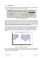
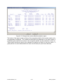
Merge Continuation Runs: This utility merges EFDC_Explorer specific output files from two
EFDC runs into a single output file. Multiple runs can be merged by starting with the
earliest runs and sequentially appending each subsequent run. At the end of each
Merge process, the EE_WS, EE_Vel, EE_WC, EE_WQ and EE_Bed from the base run
will be saved in the base run project directory, but with an “.org” extension. The newly
merged files will have the “.out” extension and can be used by EFDC_Explorer. The
models/projects must be of the same model domain and discretization.
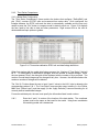
Re-sample Output: Allows the user to reduce the number of saved output snapshots in the
EFDC_Explorer output files (i.e. the EE_WS.out, EE_Vel.out, EE_WC.out, EE_WQ.out
and EE_Bed.out). At the end of the resampling process, the original output files will
have been saved in the project directory but with an “.org” extension. The newly
resampled files will have the “.out” extension and can be used by EFDC_Explorer. To
resample the output the user runs this utility and enters a snapshot skip interval. Once
the user verifies that the resampling produced the desired results, the user may want to
delete the *.ORG files to save disk space. This function can also be used to delete all
the model results after a specified time (i.e. truncate).
Modify ModChan File: This option provides access to a channel modifier global editor that
recalculates channel lengths, change orientation from U to V and vice-a-versa. It also
has a Q/A function to ensure all the upstream and downstream I & J’s point to valid cells.
The ViewPlan function allows the user a graphical point and click approach to create and
edit these “pipes”.
Categorize Bottom Shears: This utility scans the EE_WC.out file for the entire simulation period
and builds a list of categorized shears into predetermined bins. The results are
displayed in a message box and placed onto the clipboard for pasting into Excel® or
some other display/plotting package.
Compute HSPF FTables: This utility computes the data necessary for creating an FTable for
the HSPF model. It assumes that the current project has been designed to be able to
generate the necessary information for the FTable. This type of project is simply the
base model, but without the actual inflows into the domain. Instead, all the flow
boundaries have a step flow to allow the system to achieve steady state at that flow, and
then all the flows must be stepped up again to the appropriate level. Generally, this can
be done with just one upstream flow BC, but each case needs to be evaluated. After the
run is complete the EFDC results should be a series of steady state flow regimes
throughout the model domain. This utility then uses these results along with the reach
polygons to build the FTable.
DS-International, LLC.
3-9
EFDC_Explorer
3.6
Grid Tools and Utilities
The “Grid Tools” function on the toolbar contains a range of different functions and utilities that
have been needed. Figure 3-9 shows a screen capture of the current functions available under
the Toolbag.
Figure 3-9 Grid Tools functions.
Orthogonality Deviation Statistics: This utility provides summary statistics on the orthogonality
of the grid. A perfectly orthogonal grid will have a zero deviation angle at every grid
intersection. The goal during the gridding process is to produce a representative and
computationally efficient grid of the model domain with as low as practical deviation
angles (e.g. < 3 degrees). The user can view a map of the deviation angles using the
ViewPlan function.
Export Outline of Model Domain: Use this function to output a bounding polygon in the
coordinate system used by the model. The output file format is P2D. This file can be
used as an overlay in ViewPlan or imported into GIS systems.
Export Grid Cells: Use this function to export the cells by cell polygons in the coordinate system
used by the model. The output file format is P2D. This file can be used as an overlay in
ViewPlan or imported into GIS systems.
Export Model Grid for Delft's RGFGrid: Use this function to export the currently loaded EFDC
model grid out to a Delft RGFGrid formatted GRD file. This file can then be directly
loaded into RGFGrid for editing.
RGFGrid edited grids can be imported into
EFDC_Explorer by selecting “Generate New ModelImport GridDelft RGFGrid”.
Export Bottom Elevations: Use this function to export an XYZ data file at the cell center
coordinates of the bottom elevations.
I-J Map: Transpose I-J's: These “I-J Map” functions are used during the grid generationimporting process to correct any model I-J orientation issues. This function switches I to
J and J to I. If boundary conditions are already assigned, the IJ mapping is remapped to
the new IJ space.
I-J Map: Reverse Order: These “I-J Map” functions are used during the grid generationimporting process to correct any model I-J orientation issues. This function flips the
DS-International, LLC.
3-10
EFDC_Explorer
numbering direction for either the I or the J index. If boundary conditions are already
assigned, the IJ mapping is remapped to the new IJ space.
Rotate Cell Angles: This function applies a rotation to the cell rotation angles. It does not rotate
the actual cell. If using the Corners.inp file it just applies a user specified rotation to the
cell rotation matrix. In EFDC the cell’s rotation matrix is used for velocity plots and
interaction with the wind field.
3.7
Text Editor
This button on the toolbar starts the ASCII editor (configured in “EFDC_Explorer Settings”, see
Section 3.3) and directly loads certain input files for the current project. From the drop down
window the user can directly access the input files: EFDC.INP, DXDY.INP, LXLY.INP,
CELL.INP, WQ3DWC.INP, WQPSL.INP or WQ3DSD.INP. In addition, the user can select
“Other INP” to access any of the input files in the current project.
3.8
Run Model
This is the function that actually runs an EFDC project/model. It does not first save to disk the
currently loaded EFDC project prior to running. Therefore, if the user has made changes that
they desire the run to reflect, the user must first save the project.
This function actually builds a batch file, saves it in the EFDC_Explorer application directory,
and then launches the batch file. The file name is RunEFDC.Bat. This DOS batch file launches
EFDC_DS or EFDC_EPA as a DOS window with the current project directory in the Title bar.
The EFDC_DS model allows the user to pause and restart the EFDC model during a run by
pressing a key when the model’s DOS window has focus.
When EFDC_DS finishes execution, the model waits for the user to press a key to continue/exit.
However, if the user writes a custom DOS batch file using EFDC_DS and does not want the
pause function, the user must add the command line switch “-nopause” to the EXE line. For
example:
E:\Code\FORTRAN\EFDC\EFDC_DS\Release\efdc_ds_080228c2.exe -nopause
DS-International, LLC.
3-11
EFDC_Explorer
3.9
Run Times
The “clock” button provides a summary of the project’s run times in hours. As EFDC runs it
keeps track of its run time, and when the run finishes it writes the information to the file
TIME.LOG. When this button is pressed, EFDC_Explorer reads the TIME.LOG file and
provides a summary of the information. Figure 3-10 shows an example timing output. This
function is operational only for the EFDC_DS version.
Figure 3-10 Example of the model run times.
DS-International, LLC.
3-12
EFDC_Explorer
3.10
ViewPlan Viewer
The ViewPlan button of the main toolbar provides access to the utility for viewing two
dimensional (2D) plan views of the model. This function is used for pre-processing visualization
and editing of the grid, initial conditions and boundary conditions. Once the model has been run
and output files generated (see Section 7.1) ViewPlan can be used to view 2D plots, extract
model cell time series and vertical profiles and other post-processing visualizations and
analyses. Section 7 contains a more complete description of the features and use of ViewPlan.
ViewPlan has many options and features for displaying background maps (georeferenced
bitmaps), line features (e.g. shorelines), labels, measured data, model-data residuals and many
more. An example plot is shown in Figure 3-11 of Perdido Bay’s bathymetry with the 250K
scale USGS topo map in the background, a timing frame showing the Gulf of Mexico tide level
at the date/time indicated in legend and the location/ID of the defined calibration stations.
Figure 3-11 Example of ViewPlan output for the Perdido Bay water quality model.
DS-International, LLC.
3-13
EFDC_Explorer
3.11
ViewProfile Viewer
The ViewProfile button of the main toolbar provides access to the visualization of the 2D vertical
section post-processing utility of EFDC_Explorer. An example of the type of plot available is
shown in Figure 3-12. This plot shows a 2D profile of dissolved oxygen along the user defined
transect shown in Figure 3-11 (see the black dotted line) for Perdido Bay. Section 8 contains a
more complete description of the features and use of ViewProfile.
Figure 3-12 Example of ViewProfile output showing dissolved oxygen for
Perdido Bay water quality model.
DS-International, LLC.
3-14
EFDC_Explorer
4 Pre-Processor Operations
In the pre-processor section of the main form, EFDC_Explorer provides a simple user interface
to many of the commonly used options in EFDC that are stored in EFDC.INP. Some
parameters and settings are adjustable directly from this form while some others, usually some
specific subgroup, are available from buttons located on the main form.
Many of the input boxes have tips/values that pop up as the user pauses the mouse pointer
over the input box. In addition, many of the input boxes have internal range checks, but as they
are so broad as to cover a large range of applications they should not be relied upon in any way
to validate user inputs.
The ViewPlan function also provides some pre-processing features and functions that will be
described later in Section 7.
4.1
Timing, Labels and Output Options
Figure 4-1 shows the “Timing & Labels” tab. On this tab the user also sets the output options
that are available from EFDC_Explorer. The model run time, time steps, including activating
auto-stepping, and output options are adjustable by clicking on the “Modify” button.
Figure 4-1 Tab: Model Title, Timing and Output.
The Run Logging Options frame shows various check box options allowing the user to output to
the log file which can be read by EFDC_Explorer’s “Get Runtime” button on the main toolbar.
Checking the “Enable Diagnostics” causes EFDC to produce a lot of extra output files and adds
to the runtime. The diagnostic files generated depend on the EFDC options. The source code
needs to be consulted to determine the content of some of these files. These can usually be
turned off after initial model testing.
The “Project Title” is an optional label that will be displayed on plots and tables. Many of the
EFDC input files will be stamped with the Project Title and the date/time of the file creation.
The “Run Log/Notes” text box provides a readily accessible free form notepad to record
changes and notes concerning each run. If used, this can provide a complete run history during
a calibration process. For each run, it is recommended to note which prior run you are using for
the current run. For example “Run012 Based on Run011” provides a clear run path. After that
DS-International, LLC.
4-1
EFDC_Explorer
entry the user should then note any changes made to the current run. These data are stored in
an ASCII text file in each run directory called “EFDC_LOG.DS”.
Selecting the “Modify” button on this tab displays the model timing and output options available
to EFDC_Explorer (Figure 4-2). EFDC has many more output options but the majority of them
have become obsolete due to the capabilities of EFDC_Explorer.
In the “Time Options” frame the user must specify the time to start and end the run, along with
the time stepping options. “Time of Start” is the Julian day, relative to the “Beginning
Date/Time”, to begin the simulation. The “Duration of Reference Period” is used to define a
project specific meaningful period. This is often set to 24 hours to select a 1 day long reference
period. The duration of the simulation is then set by specifying the number of reference periods.
The ending time is computed from the starting time and duration.
Figure 4-2 Runtime, Output and Title.
The “Dynamic Timestep Options” subframe allows the user to enage autostepping by setting the
“Safety Factor” to a positive number >0 and <1. Generally, the safety factor ought to be less
than 0.8 but some runs work with the safety factor>1 and some require a value <0.3. The
number of Ramp-Up Loops can also be set by the user.
“Linkage to Water Quality Models” frame allows the user to bring in data from various water
quality modelling models as illustrated. The WASP models allows the user to select from EPA
DOS Ver 4, EPA DOS Ver 5.1, Tt DOS Ver 5 (Old), Tt DOS Ver 5 and EPA Ver 6.1 (Windows).
4.1.1. EFDC_Explorer Output Options
In order for EFDC_Explorer to post-process model results, the “EFDC_Explorer Output” option
must be turned on (i.e. check the “Use” check box). Which data to output is selected by the use
of the sub-item check boxes, such as “Velocities.” Water Surface must be turned on for
EFDC_Explorer to post process any of the model results.
DS-International, LLC.
4-2
EFDC_Explorer
If simulating water quality with the full sediment diagenesis option turn on, EFDC_Explorer can
display the spatial and temporal sediment fluxes and concentrations if the user enables the
“Sediment Diagenesis Data” check box. Because the sediment processes are slow, as
compared to water column processes, the user has the option to output the diagenesis data at a
slower frequency. If the output interval is >1 then the sediment diagenesis data will be output
as the frequency of “Writes per Reference Period” / “Output Interval”. As an example, if the
Reference Period is 24 hours, the “Writes per Reference Period” is 24 (1 snapshot per hour),
and the “Output Interval” is 24, then the sediment diagenesis results will be output once per day.
4.1.2. High Frequency Dates
The “Use High Frequency Dates” option is an EFDC_DS option that inserts higher frequency
output snapshots into the base snapshot frequency defined in the “Writes per Reference Period”
field above. This allows the user to use a larger base snapshot frequency, resulting in smaller
output files and faster post processing times, and still capture specific times in detail. This is
very useful when matching model results to specific sampling events.
4.1.3. Calendar/Julian Date Linkage
If the user wants to relate the model timing to actual calendar dates, the user is required to enter
a base date from which the model Julian dates will be added to compute the corresponding
Gregorian date. The use of the base date and model Julian dates allow EFDC_Explorer to
compare model versus data for a range of plots and statistics.
The base date is entered in the “Model Simulation Start Time” frame. Typically this date is the
1st of some calendar year but this is not required, any date/time is acceptable. The user can
use the “J<->G” button to convert Julian to Gregorian or visa-versa.
If using Microsoft Excel dates for the Julian day counter, the EFDC_Explorer date base should
be set to “01-Jan-1900”. This allows number formatted dates in Excel to be directly used by
EFDC_Explorer without adjustment. However, a projected oriented base date is recommended
to prevent large numbered Julian dates, e.g. 39234.375 (01-Jun-2007 09:00). If 01-Jan-2007
was used as the base date the corresponding Julian date is 151.375.
DS-International, LLC.
4-3
EFDC_Explorer
4.2
GVC (Generalized Vertical Coordinate) Options
Figure 4-3 shows the GVC and model selection options. EFDC_Explorer supports two EFDC
models, the EFDC_EPA version (with GVC) and the EFDC_DS version. When loading an
existing model, EFDC_Explorer identifies the type of model and automatically sets the options
on this tab, based on the data in the EFDC.INP file. In addition, the user can switch from one
type of model to the other using the model selection option in the “Model Selection” frame.
When changing from one model type to the other, the user should check the model layering and
boundary conditions to ensure the inputs are correct.
Figure 4-3 Tab: GVC.
When using the EPA GVC Model the GVC options are enabled. The user must specify which
layering option to use with the GVC model, either a Standard Sigma Vertical Grid (pre-GVC
layering option or a Generalized Vertical Grid (GVC) option that allows the number of layers to
vary in the model.
If the GVC layering option is selected the following sub-options must be specified:
“Use GVC Layer File”: Check to manually set the cell by cell layers. When checked the
GVCLayer.INP file is written by EFDC_Explorer and then used by EFDC_EPA during the
model run. If not checked, EFDC_EPA automatically assigns the GVC layers using the
Surface and Bottom Reference Elevations. EFDC_Explorer can set and display the
GVC layering. Use the “Initialize Layering” button to set the layering automatically, using
the Surface and Bottom Reference Elevations. You can then view, modify and reset the
layering in the PlanView function.
A GVC grid has two types of cells, Local Sigma or GVC cells. Local Sigma cells use the
number of layers specified in the “# of Vertical Layers in Sigma Region”. The number of
layers must be less than or equal to KC.
The Utility Options frame allows the redistribution of the total flow into the active layers for all the
flow type Boundary Conditions by pressing the “Distribute BC Flows” button. When using the
GVC Grid, the “Initialize Layering” button allows the user to initialize the GVC layering using the
Surface and Bottom elevations specified in the Reference Elevations form.
The Surface and Bottom Reference Elevations should initially be set to something near the
maximum water surface elevation and minimum bottom elevation, respectively. These can be
altered at any time and the layering recomputed using EFDC_Explorer to determine their
validity. The validity of the layering can be viewed in the ViewPlan function, under “Fixed
Params” viewing option.
DS-International, LLC.
4-4
EFDC_Explorer
4.3
Grid & General
Figure 4-4 shows the “Grid & General” options tab. This tab has a range of different types of
inputs which are examined below.
Figure 4-4 Tab: Grid, numerical solution and miscellaneous options.
The “Water Layers” frame shows primary water layer settings (KC = number of water layers)
and the distribution of the relative layer thicknesses. The relative thicknesses must add to 1 (or
very close). EFDC_Explorer checks this for the user. EFDC_Explorer will automatically divide
the water layers into an equal fractions based on the number of layers specified by the user.
Note that layer 1 is the bottom most layer and that the highest layer number is the surface layer
(i.e. KC).
A feature here that is very useful during preliminary testing of a model application is the rapid
adjustment of layering simply by changing the number of layers. EFDC_Explorer simply
reallocates the layering based on the new KC and then adjusts all the boundary conditions to
reflect this change. Use this feature with care, but it has been tested on several applications
and found to work well.
“Run Time Status” frame contains the settings for EFDC’s feedback to EFDC’s runtime screen
during the model run. The user can simply type in the desired I and J or the user can set them
using the mouse. To set using the mouse, select “ViewPlan/Cell Map” or “ViewPlan/Bottom
Elev” views, then right mouse click on the desired cell and select “Set as Show I J”. The data
displayed on the screen depends on the “Type”, whose options are: Salinity (1-special, 2-N, 3time), 4-Temperature, 5-Cohesives, 6-Non-Cohesives, 7-TSS, 8-Dye/Age.
The “Wetting and Drying” frame uses a flag to select various options. These options can change
depending on the model settings. Generally, setting the flag to ISDRY=0 turns off wetting and
Note
If any of the “multiplicative factor” settings for water
depth or bottom elevation are 0 (or blank), EFDC
will compute a zero for that parameter for the
initial conditions.
drying; ISDRY=1 turns wetting and drying on (with constant HWET), ISDRY=2 turns wetting and
drying on (with variable HWET), ISDRY=11 is the same as ISDRY=1 but with no non-linear
iterations, ISDRY=12 is the same as ISDRY=2 but with no non-linear iterations, and ISDRY=99
DS-International, LLC.
4-5
EFDC_Explorer
is the latest algorithm for multi-face wetting and drying. If ISDRY is a negative of the flag (e.g. 99) then EFDC uses cell skipping to improve computational speed. Most applications that need
wetting and drying should use ISDRY = -99.
When using wetting/drying the “Minimum Height” in the “Water Depth Setting” frame should be
less than the “Dry Depth”. Otherwise, the initial water depths everywhere will force all of the
models cells to “wet”, even if they should be dry.
The “Mass Balance” frame enables mass balance checking and reporting for EFDC. The
number of steps relates to the number of time steps accumulated between reporting. The “V”
button provides quick access to the mass balance file. Consistent with the fixed naming
convention, the mass balance file written by EFDC is BAL.OUT for the 3 time level solution and
BAL2T.OUT for the 2 time level solution.
With the “Masks” frame the “Use” check box enables the user to enable masks (zero thickness
flow barriers) in EFDC. The MASK.INP file will then be required by EFDC. EFDC_Explorer can
generate and modify masks using the “Modify” button as shown in Figure 4-5. The “Create
Masks” utility does not automatically turn on the mask computation, it just generates the masks
and writes the MASK.INP file. The user must manually click the mouse cursor inside the “Use
Masks” check box to use the masks generated.
Masks can be viewed, added and deleted in the ViewPlan function. When viewing the Bottom
Elevations, RMC on a cell (“Enable Editing” must be checked first) and the cell properties are
displayed, along with the mask options.
Figure 4-5 Mask Editing Tool.
DS-International, LLC.
4-6
EFDC_Explorer
4.4
Computational Options
The “Comp Opts” tab is shown is Figure 4-6. This tab provides access to the main
computational options for EFDC. The “Computational Options” frame provides access to the
computational and transport switches and options that are contained in C6 in EFDC.INP. These
switches are the primary activation switches to specify which state variable(s) will be simulated
by EFDC.
Figure 4-6 Tab: Computational Options.
If the user has elected to “Activate Temperature” then the drop down list provides several
options, including: Atmospheric linkage, Full Heat Balance, External Equilibrium Temperature,
Constant Equilibrium Temperature and Equilibrium temperature (CE-QUAL-W2 method,
EFDC_DS only). The “Global Transport Options” subframe allows the user to select from
Upwind Difference, Central Difference and Experimental Upwind, as well as to use AntiDiffusion or Anti-Diffusion Correction methods.
The “Numerical Solutions Options” frame provides access to several of the numerical solutions
schemes available in EFDC. Most of the recent development and testing has been made using
the conjugate gradient solver. Solution schemes available are Standardized (0), Ordered R/B
Conjugate gradient (2), reduced R/B Conjugate gradient (3), and Conjugate gradient for Wetting
and Drying (9). Internal Buoyancy forcing options can also be selected.
The “3 Time Level” (3TL) or “2 Time Level” (2TL) Options allow the user to select the method to
be used for numerical simulation. If using the EFDC_EPA model with GVC layering, the Time
Level must be “3 Time Level”.
If using the 2TL solution the “Momentum Equations Solution” frame allows the user to choose
between explicit and implicit solution options.
If using the 3TL option, the user must specify the momentum solution option (ISCDMA) of
Upwind, Central, and Upwind following the MOM momentum advection scheme. There are
other schemes (ISCDMA>2) that are experimental.
DS-International, LLC.
4-7
EFDC_Explorer
4.5
Hydrodynamics
Figure 4-7 shows the “Hydrodynamics” tab and the various options available to the user. Each
of the sub items are discussed below.
Figure 4-7 Tab: Hydrodynamics.
The “Ramp Up Options” frame in the lower left hand corner allows the user to modify the timing
to full transition physics. Buoyancy can be adjusted with a Buoyancy factor that must be
between 0 and 1, with 0 being no buoyancy influence and 1 being full buoyancy influence. For
some applications, the ramp up time from the ICs to natural physics require the phasing in of the
buoyancy and the non-linear terms. This is accomplished using the “Modify” button and
applying some ramp up settings.
The “Coriolis Effect” frame allows the user to determine the Coriolis number by setting the
“Latitude (Deg)”, which is the latitude of the midpoint of the model domain.
The “Channel Modifiers” frame allows the use to select the use of EFDC channel modifiers.
These are like “pipes” that connect two cells. The “Channel Modifier Flag” option box is used to
enable the use of the channel modifiers capability of EFDC. The normal “on” option is when this
flag is set to 2. If set, EFDC requires the MODCHAN.INP file to be input. The most flexible
approach to create and edit channel modifiers is to:: 1) turn on this option (i.e. ISCHAN=2), 2)
enter the ViewPlan, 3) select “Modchannel”, 4) enable edit, and 5) use the right mouse click to
add, delete or modify channel modifiers (i.e. “pipes”). Care should be exercised in using
channel modifiers as model instability is sometimes increased and mass balance errors can
occur.
4.5.1. Turbulence Options
The “Turbulence Options” frame displays the various hydrodynamic parameters like eddy
diffusivities and activation of wave generated turbulence which can be selected and changed by
clicking on the “Modify” button. These options are described in the follow sub-sections.
4.5.1.1 Turbulent Diffusion
Figure 4-8 shows the main form for the computational options for the horizontal and vertical
eddy viscosities and diffusivities. The parameters and options have been grouped according to
which dimension they are used for, i.e. horizontal or vertical.
DS-International, LLC.
4-8
EFDC_Explorer
Figure 4-8 Eddy Viscosities & Diffusivities.
The resulting horizontal diffusivity from these options can be viewed from within ViewPlan if
velocities are also available. The vertical eddy viscosities and diffusivities (AV & AD arrays in
EFDC, respectively) can also be viewed if the user configures the Internal Array Viewer (See
Appendix A) to include these arrays.
4.5.1.2 Turbulent Intensity
Figure 4-9 shows the Turbulent Intensity tab. Generally, only the Vertical Turbulence options
will be changed. At the current time, production runs should set the “Advection Scheme” to 1
and the “Sub-Option” to either 0 or 1. The “Turbulence Closure Constants” should not be
changed without good justification.
Figure 4-9 Turbulent Intensities.
DS-International, LLC.
4-9
EFDC_Explorer
4.5.1.3 Wave Generated Turbulence
EFDC_Explorer has several options for generating wave effects, as shown in Figure 4-10 and
Figure 4-11. Most recently EE has been enhanced to include the ability to internally generate
wind wave bed shears (ISWAVE=3). This option allows simulation of wave effects and resuspension of sediments inside EE.
Using this option, a wind time series is used to provide the instantaneous values of wave
parameters with fetch calculated for each cell in eight directions. This is used to calculate total
bed shear stress, with bed shear stress linked to the current via the Grant Madsen approach.
This option means that it is no longer necessary to use imported external wave turbulence to
simulate wave propagation (Dang Huu Chung and P.M.Craig, 2009). The fetch for each sector
for which the wind is blowing may be viewed in ViewPlan (see Section 7.6, “ViewPlan Main
Viewing Options”).
The “Wave Parameter & Options” form allows the user to specify “Ks,” which is the Nikuradse
sand roughness value. This can be estimated as Ks = 2.5 x d50.
Figure 4-10 Wave Turbulence Tab: Internally Generated Wind Waves.
Alternatively, EFDC also the ability to import wave generated turbulence from
wave models, such as REF/DIF1 Ver 2.5 (1994) (Figure 4-11). These imported
stresses can then be used to either impact only the boundary stresses (for
sediment transport, ISWAVE=1) or can be used to impact the flow field and
boundary layer (ISWAVE=2). DSLLC has tested and verified this option for
both EE and EFDC using the RefDif/ShoreCirc modeling of rip tide currents
(Svendsen, et. al., 2000).
DS-International, LLC.
4-10
Wave Properties
to be imported.
EFDC_Explorer
Figure 4-11 Wave Turbulence Tab: Wave Options.
Figure 4-12 shows the main import/field interpolation form for the wave parameters. The user
must match the input data file (which should be in XYZ format tab, space or comma delimited)
to the parameter drop down list “Wave Field Parameter” (options shown in adjacent inset). The
user can either have wave height (2*wave amplitude) or wave energy, EE will compute the one
from the other. The user has the option of using a polygon to select which EFDC cells will be
used for the assignment. If a Poly file is not selected, then the assignment operation will be for
the entire model domain. EE interpolates and converts the wave model results into the formats
needed for EFDC. The interpolation process has two options, nearest neighbor interpolation or
cell averaging. Cell averaging should be used when the imported data is denser than the EFDC
model grid (this will usually be the case). The nearest neighbor interpolation scheme should be
used if the imported data is sparser than the EFDC model grid. An example of the XX
component of the radiation shear stress is shown in Figure 4-13.
Figure 4-12 Wave generated turbulence, import data form.
DS-International, LLC.
4-11
EFDC_Explorer
Figure 4-13 Wave parameters: Radiation shear stress XX component.
4.5.2. Roughness Options
Under “Roughness Options”, other than the standard additive and multiplicative factors that
EFDC will apply to whatever z0’s are input in the DXDY.INP file, EFDC_Explorer has several
methods to set and/or modify the z0’s that will be written in the DXDY file.
“Floodplain Z0’s” and “Channel z0’s”: If the model was constructed with channel and floodplain
cell ID’s (i.e. 5 for channels and 7 for the floodplain in the cell map file, i.e., cell.inp) then the
user can set each one quickly using these buttons.
“Polygon Set”: The user can use a user defined polygon to modify/set the z0’s. This tool may
be applied as many times as needed anytime during the model construction and calibration
process.
DS-International, LLC.
4-12
EFDC_Explorer
4.5.3. Vegetation
In the “Vegetation” frame on the main form the user can set the primary computational option for
enabling the feature and at what level (see the tooltips). The vegetation class settings are
available via the “Modify Classes” button option which provides a user interface to the data that
are needed for the VEGE.INP file (Figure 4-14). First, the user should specify the number of
vegetation classes needed. Enter the number of the “Number of Vegetation Classes” into the
input box and press return. The grid will be expanded to accommodate the desired number of
classes. All of the inputs required by EFDC are shown with a couple of exceptions. The Beta1
and Beta2 variables are actually not used but are included in the list. The VEGE.INP file must
have data in those columns but they are not actually used by EFDC. The other exceptions are
the ID and Description fields. They are only used by EFDC_Explorer. The ID field is used to
match vegetation classes to polygon ID’s (see the following description of “Apply Overlays”) to
automatically set the vegetation map that is needed for input via the LXLY.INP file. The
Description field is only used for labeling.
Figure 4-14 Vegetation class parameters.
The “Apply Overlays” button uses the vegetation class ID field and matches it to input polygon
ID’s. Figure 4-15 shows the form for applying a vegetation map to the model cells. The file
containing one or more polygons in the same file (see Appendix B for polygon formats) needs to
be opened (via the “Browse” button). The polygon file will be read and the polygon ID’s will be
matched to the vegetation class ID’s. If any vegetation classes do not have any defining
polygons the user will be notified. Once the initial matching process is complete the user then
must choose to perform the actual vegetation assignment. If there are unmatched vegetation
classes, the user can choose to process anyways but they need to be aware that no EFDC cells
will be matched to any the vegetation classes that do not have a polygon. The classes can
always be edited later, if desired. Figure 4-16 shows a vegetation map that resulted from the
polygon/vegetation class assignments.
A simpler approach can be used to assign a single vegetation class to a polygon region if the
P2D file contains only one polygon.
DS-International, LLC.
4-13
EFDC_Explorer
Figure 4-15 Cell property assignments: Vegetation map with IDs.
Figure 4-16 Example vegetation map assignment.
DS-International, LLC.
4-14
EFDC_Explorer
4.6
Sediment, Toxics and Other Parameters
Figure 4-17 shows an example of the “Sed/Tox/Others” tab which allows setting for sediment,
toxics, dyes, tracer tools and heat/temperature. Each of the major sections is discussed in the
following subsections.
Figure 4-17 Tab: Sed/Tox/Others.
4.6.1. Sediments
The sediment transport parameters and options are set using the forms shown in Figure 4-18 to
Figure 4-23. The principal settings for the number of sediment classes and bed layers are
specified in the top frame under “Major Settings”. As with the toxics, these “Major Settings”
parameters should only be changed with care and usually early in the model calibration process
so as not to lose your initial and boundary conditions.
Figure 4-18 shows the form with the “General” tab shown. On this tab the user can tell EFDC
whether or not to simulate cohesives and non-cohesives and the approach to compute bed
shear stresses for sediment transport. Un-checking the “Simulate Cohesives” and/or “Simulate
Non-Cohesives” check box does not delete previously defined sediment transport parameters.
The “Sediment Timestep” is a multiple of the number of hydrodynamic time steps to calculate
between each sediment bed process computation (i.e. deposition, erosion, consolidation, etc.).
Because the bed processes are slow, relative to the hydrodynamics, this number can often be
10 or greater. The user should conduct testing by starting with a low number and increase the
Sediment Timestep until the user detects a noticeable difference in the model results. Then the
number should be reduced by some amount in order to provide a safety factor. This can then be
used for the subsequent calibration and production runs.
The “Bed Shear Calculation Options” allows the user to choose from a number of different
calculation options for bed shear stress computations.
DS-International, LLC.
4-15
EFDC_Explorer
Figure 4-18 Sediment Transport – General.
Figure 4-19 shows an example of the “Cohesives” tab in the Sediment Transport form. For
many of the fields in the “Erosion & Deposition Parameters” grid, clicking on a cell and pressing
F1 pops up helpful information for that field.
The number of columns shown in the input parameter grid varies with the number of classes to
be modeled. The Diameter setting located at the bottom of the parameter grid sets the grain
size that will be used in calculating d50’s for the sediment bed. It is not used for any other
calculations.
Figure 4-19 Sediment Transport – Cohesives.
DS-International, LLC.
4-16
EFDC_Explorer
Figure 4-20 shows the form with the “Non-Cohesives Suspended” tab shown. It is similar in
function and operation to the cohesives tab. Grain size for each non-cohesive class is required
for the sediment transport computations. This value is also used as the grain size for the d50
calculations. A number of options for computing equilibrium concentrations are available in the
“Equilibrium Conc” frame. This includes the option of equilibrium concentrations calculated from
Sedflume data with or without critical shear stress. Setting the settling velocity or the critical
shear stress values to numbers <0 results in EFDC computing those parameters values using
the Van Rijn equations (1984a, 1984b).
Pressing F1 for help pops up information relevant to the current input field.
The “Sediment Info” button provides a sediment properties calculator. Pressing the “Set
Parameters” button will initialize the sediment properties using the Van Rijn equations if the
sediment diameter is specified prior to pressing the button.
Figure 4-20 Sediment Transport – Non-Cohesives Suspended.
DS-International, LLC.
4-17
EFDC_Explorer
Figure 4-21 shows the tab for the “Non-Cohesives Bedload.” The use of the Gamma parameters
is slightly different between the different EFDC codes. The user should know how the Gamma’s
are used by reviewing the code prior to finalizing the desired inputs.
Pressing the “Initialize Constants” button will bring up a dialog box asking the user to select the
bedload approach to use. EFDC_Explorer sets the bed load transport constants to standard
literature values for the computational approach selected. The user should know how the
Gamma’s are used by reviewing the code prior to finalizing the desired inputs.
Figure 4-21 Sediment Transport – Non-Cohesives Bedload.
DS-International, LLC.
4-18
EFDC_Explorer
Figure 4-22 shows the tab for the “Bed & Consolidation” of the sediment properties option. In
this tab the user may specify various bed consolidation and bed morphology settings.
The “Bed Morphology Options” form allows the user to choose between no bed changes (option
0) and allowing bed elevation changes (option 1). The “Max. Water Depth” is the maximum
allowable depth to allow for the “lost” due to “NEG DEPTH” morphological change (EFDC_DS
version only).
Bed Consolidation & Mechanics Options frame provides input to the main sediment bed
consolidation options. The “Bed Mechanics” option must be 0-None, 1-Simple, or 2-Finite
Strain. Option 2 is very a specialized approach and requires a detailed understanding of the of
the Finite Strain implementation in the FORTRAN code. The consolidation rate is in seconds,
not 1/seconds as earlier versions of EFDC.INP reported. The rate will usually be >100000
seconds. The impact of the rate of consolidation can easily be tested using EFDC_Explorer’s
“Single Column Sediment Layers” post-processing function (see Section 5.2.1).
Figure 4-22 Sediment Transport – Bed and Consolidation.
DS-International, LLC.
4-19
EFDC_Explorer
Figure 4-23 shows the sediment parameters form with the “Initial Conditions” tab selected. On
this form the user selects how they would like to initialize the bed sediments for the model. This
is done by selecting the option from the “Sediment Initial Conditions Options” frame.
Figure 4-23 Sediment Transport – Initial Conditions.
To set up a simple horizontally uniform sediment bed for the model the user can select
“Create Uniform Bed” option. This brings up a dialog form that asks the user to input
number of layers, the number and types of sediments, and allows the user to specify
sediment fractions, thickness, and bulk densities for each layer. The user must still set
cohesive and non-cohesive erosion & deposition parameters, but once the user finishes
option, the sediment bed configuration is ready for EFDC.
the
the
the
the
this
Figure 4-24 shows the uniform sediment bed generator. This utility allows the user to specify
the thickness, porosity (thus void ratio) and mass distribution by layer. Once the sediment bed
is generated the user can modify the sediment bed properties in ViewPlan, as needed. The
layer configuration settings can be saved and later retrieved using the “Save” and the “Load”
buttons in the “Bed Properties Definitions” frame.
DS-International, LLC.
4-20
EFDC_Explorer
Figure 4-24 Uniform sediment bed generation tool.
4.6.2. Steps To Set up a Sediment Bed Model:
1. Enter the “Sed/Tox/Others” Tab and click on the “Sediment and Sediment Bed Settings”
button
2. Define the number of sediment bed layers, cohesive and non-cohesive sediments as
shown in “Major Settings” of Figure 4-18 (it is important do this first to avoid losing data).
3. Set the options in the “General” tab for the “Primary Computational Options” and the
“Bed Shear Computation Options”.
4. In “Cohesive” Tab the user should enter the appropriate values for the relative
parameters as well as defining the minimum and maximum values of Cohesive Fluids
Concentration as shown in Figure 4-25.
Figure 4-25 Sediment Bed Model: Cohesives Tab.
5. In the “Non-cohesive Suspended Load” Tab the user should define the Equilibrium
Concentration Option and enter the appropriate values for the relative parameters and
non-cohesive layers.
DS-International, LLC.
4-21
EFDC_Explorer
6. In the “Non-cohesive Bed Load” Tab the user should click on “Initialize Constants” button
and enter the number for the approach desired e.g. enter “1” for the Van Rijn approach.
7. In the “Bed & Consol” Tab the user should select the Bed Morphology Options: 0-No
Bed Change, 1-Allow Bed Changes. The user should also set the Max Layer Thickness
and Constant Porosity to be the same values as in the input sediment file (refer to
Appendix B-9 for the DSM format of the file).
8. In the “Initial Conditions” Tab: select the Sediment Initial Condition Options. There are 2
options to initialize bed layers: Uniform bed and use initial data file.
9. Initialize the sediment bed from file, browse for the input sediment file
10. Check “Use sediment cores” with grain size
11. Define the maximum grain size for each size class relatively to cohesive and noncohesive layers as displayed in the in the red frame in Figure 4-26.
12. If the required information has been entered then the “Apply” button is visible. After
clicking on Apply, the sediment bed will be initialized.
Figure 4-26 Tab: Sediment Bed Model: Initial Conditions Tab.
4.6.3. Digital Sediment Model
A very useful feature in EFDC_Explorer is its ability to build the EFDC sediment files from a
defined digital sediment model (DSM) that was generated by some third party package (e.g.,
Spatial Explorer). The DSM format requires a polygon followed by the layer thickness, bulk
density, porosity and grain size distribution for each depth available (sediment depth intervals
are based on data). More information on the data structure is available in Appendix B.
EFDC_Explorer uses the DSM coupled with the number of size classes requested, the
maximum size for each class, the number of sediment layers and the layer options (e.g.,
minimum layer thickness) to build the EFDC sediment files. The “Max (μm)” sediment
diameters, one for each sediment class, are needed to break the sediment grainsize curves into
ranges. These diameters are not the class diameters but represent the grainsize breakpoints
DS-International, LLC.
4-22
EFDC_Explorer
whose geometric mean of the upper and lower limits is the corresponding sediment class’
diameter.
When the user clicks on the “Apply” button after all the inputs have been provided,
EFDC_Explorer generates the sediment map in memory and then writes out the files. The
current sediment map (if any) will be replaced by the new one. It is recommended that the
project be saved into a new subdirectory prior to implementing this option in order to save
different versions of the sediment bed configurations.
Figure 4-27 shows an example of a digital sediment model derived from sediment cores. The
data contained grainsize distributions by depth interval. The black diamond symbols show the
locations of the cores. The plot shows the resulting depth averaged d50 grainsize.
Figure 4-27 Example digital sediment model generated from sediment cores with grainsize.
DS-International, LLC.
4-23
EFDC_Explorer
4.6.4. Toxics
The toxic transport parameters and options are set using the form shown in Figure 4-28. The
number of toxics included in the simulation are displayed in the top frame titled “Major Settings”.
This can be changed by the user, but since boundary and initial conditions are predicated on the
number of toxics, changing this value resets many of the toxics inputs. Therefore, this should
only be changed when the user is prepared to reset all the initial and boundary conditions. A
special case here is if the user sets the number to 0; then the toxics inputs are skipped for that
project from that time forward.
Figure 4-28 Toxic Transport Options.
To enable the simulation of Toxics you need to select “Compute Toxics” checkbox or set the
simulate toxics (ISTRAN(5)) flag to 1 under the “Grid & General” tab, “Computational Options”
button.
Each toxic has many of its own settings so the user must first select the toxic to be
edited/entered by using the drop down list in the upper left corner of the “Toxic Transport
Parameters” frame. Once a toxic has been selected all the appropriate information is displayed
on the form. The “Toxic Name” field is only used by EFDC_Explorer for labeling and
information. The contents of the grid (i.e., field) under the “Partition Coefficients” changes
based on the partitioning model selected.
The partitioning factors and the concentration factors units must be consistent. Typical units for
the toxic concentrations are mg/kg or μg/kg.
DS-International, LLC.
4-24
EFDC_Explorer
4.6.5. Dye
If the Dye computational option is selected then the user may assign a “decay” rate to the
otherwise conservative tracer. The “decay” rate options are shown in Table 4-1.
Table 4-1 Dye “decay” rate options.
Dye
“Decay”
Rate
>0
0
<0
1000
EFDC_DS Operation
First order decay rate
Conservative tracer
First order growth rate (EFDC_DS Only)
The “dye” constituent is used as an “Age of Water” function to
compute residence times and visualize domain/boundary water
mixing. (EFDC_DS Only)
Depending on the decay rate option, the user can view and animate the dye concentrations or
“Age of Water” in ViewPlan.
If using the restart option, the user can initialize a dye field using the DYE.INP file by selecting
the “Dye Overwrite” check box on the “Initial” tab, located in the “EFDC Restart Option” frame.
4.6.6. Heat Temperature
To activate the heat sub-model in EFDC, the “Temperature” constituent must be activated
(“Computational Options” frame on “Comp Opts” tab). The ASER.INP file must be used for all
of the thermal sub-models to compute the surface and bottom heat exchange processes.
Depending on whether the current model is EFDC_EPA or EFDC_DS, the EFDC_Explorer form
will have different options shown in the “Heat/Temperature” frame. The following provide an
overview of the approaches.
The EFDC_EPA model uses a new thermal bed model to determine the bed/water column heat
exchange (Tetra Tech, 2007c). A sediment thermal thickness is assigned for the entire model.
This thickness is not related to either the sediment transport model’s bed or the water quality
sediment bed. This thermal layer is then divided into KBH layers (must be >2). A constant
initial bed temperature can be used or alternatively the TEMPB.INP file can be used to assign a
spatially variable initial temperature, by layer. Check the “Use TEMPB.INP” checkbox in the
“Bed Thermal Options” frame for this option.
The EFDC_DS version of the model has two different approaches for the bed heat sub-models.
If the standard EFDC full heat balance (ISTOPT(2)=1) sub-model is used, the water/sediment
bed heat exchange model of the pre-GVC version is used. If the user has selected the
equilibrium temperature sub-model (ISTOPT(2)=4) then the bottom heat exchange is computed
using the heat exchange coefficient and the user can assign spatially varying sediment
thicknesses and initial temperatures using the TEMB.INP file.
DS-International, LLC.
4-25
EFDC_Explorer
Various atmospheric parameters can be adjusted using the “Modify” button in the
“Heat/Temperature” form. An example of the “Atmospheric Parameters” values box is shown in
Figure 4-29. The parameters shown in Figure 4-29 change slightly depending on which heat
sub-model is being used.
Figure 4-29 Atmospheric Parameters.
4.6.7. Tracer Tool
The purpose of the tool is to provide a quick way to setup EFDC computational options and
boundary conditions for point source tracer injections. Figure 4-30 shows an example of the
tracer tool. The list in the upper left of the “Dye Injection Point” frame shows the tracers
currently defined. The list on the right is a listing of all the currently defined flow type cells. The
user needs to assign an existing cell or create a new dye injection point and then assign the
flow and dye concentration for each point.
DS-International, LLC.
4-26
EFDC_Explorer
Figure 4-30 Tracer generation tool.
To define an existing boundary cell as a tracer, select the cell from the list on the right and press
INS to add it to the tracer list. You must then define the flow and dye injection characteristics for
each tracer cell. You can delete tracers by selecting the cell on the left and pressing DEL.
4.7
WQ – General
The water quality tabs of “WQ-General”, “Benth/Nutrients” and “Algae/WQ ICs” provide the user
with a graphical user interface to the water quality sub-model of EFDC, sometimes called
HEM3D (Park, et.al. 2000). The implementation of the water quality varies between versions of
EFDC so the user should be aware of what is contained in the source code for their particular
version of EFDC.
The “WQ - General” tab is shown in Figure 4-31. Some of the user options include setting the
Global Kinetic Options from one of several modules. For the EFDC_EPA version, the standard
kinetic model is contained in Module 3 (ISWQLVL=3). While the other kinetic modules may be
used (with care) when using the EFDC_EPA version in the standard sigma mode, if the GVC
option is selected ONLY module 3 works. For the EFDC_DS version, the standard full kinetic
module is Module 1 (ISWQLVL=1). Once the kinetic option has been chosen the user still
needs to select which parameters will be varied/simulated within the selected kinetic option.
Clicking the “Params” button brings up the list of parameters whose simulation (i.e. advection
and dispersion) can be switched on or off. However, even if a parameter is not simulated, since
it is still part of the kinetics, the IC concentration is used for all of the kinetic calculations.
The best way to initialize the water quality sub-model is to initialize the current model using data
from another EFDC_Explorer model. This is done using the “Initialize WQ Parameters from
File” in the “Miscellaneous” frame. This operation should only be conducted once at the start of
the water quality model construction. This process overwrites all of the current model’s settings.
EFDC allows for water column zones for the assignment of many of the water quality
parameters. The WQ zones can be set using the “Define Zones” button or can be set in
ViewPlan (Water Column/Wtr Quality then check “WQ Zones” checkbox). Clicking on the
“Define Zones” button brings up the “Apply Cell Properties via Polygons” form. You must first
DS-International, LLC.
4-27
EFDC_Explorer
enter the maximum number of desired zones in the “Number of Kinetic Zones” box.
number can be changed at any time during the model building process.
This
Zones are assigned by water column layer and cell, so it is possible for the same cell to have
more than one zone assigned to it, if KC>1. The parameters that vary by zone are shown in the
frame “Water Quality Kinetics”. There are three groups of parameters that can vary by zone.
The each group, the use of zones or not is separately controlled using the check boxes for that
group. The specific parameters for the “Current Zone” for each group are modified by clicking
on the “Modify” button.
Figure 4-31 Tab: Water Quality – General.
4.8
Benth/Nutrients
The “Benth/Nutrients” tab, shown in Figure 4-32, provides access to the sediment
diagenesis/benthic flux settings as well as many of the basic nutrient parameters. The nutrient
parameters have been grouped by nutrient type and can be edited by clicking on the respective
button. For example to edit the Nitrogen settings the user would click on the “Nitrogen” button.
Figure 4-32 Tab: Benth/Nutrients.
The atmospheric wet deposition concentrations for the constituents being simulated with the
kinetic module selected are edited via the “Wet Deposition” button. The dry deposition mass
fluxes are edited via the “Dry Deposition” button.
The nutrient benthic flux computational options are set using the “Modify Parameters” button in
the “Benthic Flux” frame. Clicking the button brings up the form shown in Figure 4-33. The top
frame, “Benthic Nutrient Flux Method” is the option that controls EFDC’s benthic flux approach.
If the nutrient mass fluxes are to be specified, either as constants or variable in time and space,
DS-International, LLC.
4-28
EFDC_Explorer
then the diagenesis tabs are not used. If the “Full Diagenesis Model” (DiToro & Fitzpatrick,
1993) option is selected then the three diagenesis tabs are available to allow the user to specify
the diagenesis parameters.
Figure 4-33 Sediment nutrient flux – Sediment Diagenesis Options and Parameters.
Figure 4-34 shows one of the diagenesis tabs for defining the diagenesis parameters. The best
way to initialize all of the diagenesis parameters is to use the “Load Settings” button. This will
read an existing WQSD3D.INP file from another project and initialize the settings for the current
project with those from the loaded project. After the user initializes the parameters they can
modify the settings during the model development stages. The diagenesis values from the
Chesapeake Bay ICM application (Cerco & Cole, 1995) provide a good starting point for
diagenesis model parameterization.
Figure 4-34 Sediment Diagenesis: Diagenesis – Options.
DS-International, LLC.
4-29
EFDC_Explorer
In addition to the diagenesis kinetic parameters, the sediment bed diagenesis initial
concentrations also need to be specified. This can be accomplished by applying measured data
for each parameter using the “Spatially Varying IC’s” button. When pressed, the form shown in
Figure 4-35 is displayed. For each of the required parameters, the user can interpolate the data
onto the model. Each nutrient reaction class, i.e. G1 (most reactive), G2 and G3 (least reactive
or inert) must be separately specified. The “Operator” can be used to factor or otherwise modify
the interpolated field or a previously defined IC field. The data can be interpolated for the entire
model in a single operation or using only selected cells by specifying a “Poly File”.
The user can initialize the spatial field to a set of constants using the “Initialize to Constants”
button. It should be noted that the sediment diagenesis bed is not linked in any way to the
sediment transport sub-model bed definition, scour or deposition processes.
Figure 4-35 Sediment Diagenesis: setting the initial conditions.
The diagenesis kinetic parameters can be divided into zones. Figure 4-36 provides access to
setting the zones and assigning the zone specific parameters. The maximum number of zones
needed is set by entering the appropriate number in the “# of Zones” field. To edit a specific
zone, the user should scroll to the desired zone using the up/down arrow control.
The zones and the zone specific parameters can be viewed and editing using the ViewPlan by
selecting the View Option “Diagenesis”, then checking the “Show Zone” option. If the “Enable
Edit” is checked, then RMC’ing on a cell allows the user to edit the cell’s corresponding
diagenesis zone’s kinetic parameters. The cell’s diagenesis zone assignments can be edited
using the Property Copy function.
DS-International, LLC.
4-30
EFDC_Explorer
Figure 4-36 Sediment Diagenesis: Diagenesis kinetic zones.
4.9
Algae/WQ IC’s
Figure 4-37 shows the tab for “Algae/WQ IC’s” (Algae/Water Quality Initial Conditions). The
“Algae Options” frame contains several buttons that, if pressed, allow the user to make
adjustments to logical parameter groups. For example the “Algal Dynamics” button brings up a
form as shown in Figure 4-38. This allows the user to modify the algal default or “background”
algal growth rates.
Figure 4-37 Tab: Algae/ WQ IC’s.
DS-International, LLC.
4-31
EFDC_Explorer
Figure 4-38 Algal Dynamics parameter form.
In the “Initial Conditions” frame the user is able to select spatially constant or spatially varying
initial conditions for each of the water quality parameters. To set spatially varying initial
conditions for the water quality parameters the user must interpolate data onto the model cells
using the “Apply Cell Properties via Polygons” utility. If the EFDC model uses spatially varying
IC’s, then the user must specify which input data format to use, i.e. WQWCRST.INP or the
WQICI format. EFDC_Explorer will generate the IC’s in the format specified. Pressing the
“Initialize IC’s” button assigns the entire domain for all parameters to the values specified as the
spatially constant IC’s.
The user can later edit (“Enable Edit” must be checked) any of these IC fields using ViewPlan.
To access the data the user should select “Water Column” as the main Viewing Option then
“Water Quality” as the sub-option, then select the parameter desired.
DS-International, LLC.
4-32
EFDC_Explorer
4.10
WQ BC / LPT
A new feature of EFDC_Explorer is the ability to be able to define Water Quality Boundary
Conditions with Load Concentrations rather than Mass Loading files. As well as this a new
Lagrangian Particle Transport (LPT) sub-model has been added. The tab that allows the user to
select from various options for Water Quality Point Source Loading and LPT is shown in Figure
4-39.
Figure 4-39 Tab: Water Quality Boundary Conditions and Lagrangian Particle Tracking.
4.10.1. Water Quality Point Source Loading
The “Water Quality Point Source Loading Option” provides a drop down table with the following
three options: “Use Constant Point Source Loads”, “Use Time Variable Point Source MASS
Loadings”, and “Use Time Variable Point Source Concentrations”.
EFDC_Explorer previously only used the larger Mass loading files. The new “Load
Concentrations” option provides the user with smaller files and greater control. When the user
selects an option different to that previously selected, EFDC_Explorer informs the user of the
current BC and asks whether they want to switch to the new option. If the user responds
affirmatively then EFDC_Explorer will convert and save out the option selected.
With the aid of the “Import & Convert WSPSLC.INP” button the user can either overwrite or
append a new Water Quality Time Series, which is a Load Concentration file, with concentration
in kg per day. The WQ BC Load Concentrations rely on two new input files: wqpslc.inp and
wqpsl.inp. Note that wqpsl.inp is an EFDC_Explorer file, and is not used by EFDC. It is often a
very large file.
When the user returns to edit the Water Quality Tables and Series in the “Boundary” tab
EFDC_Explorer displays all 21 WQ parameters. In the MASS Loadings option these parameters
are depth averaged and not layered, and so are vertically constant. However, after converting to
Concentrations loadings, the user is informed that the values have been converted, and now are
now stored layer by layer. Initially these values will be an average as calculated by
EFDC_Explorer, but the user can now specify certain layers and assign new values as required.
DS-International, LLC.
4-33
EFDC_Explorer
4.10.2. Lagrangian Particle Transport (LPT)
EFDC_Explorer has been updated to incorporate the pre- and post-processing of LPT’s (Dang
Huu Chung and P.M.Craig. 2009). The EE pre-processing provides full control for initial particle
seeding, LPT computational option selection and plotting. The EE post-processing allows for a
range of display options for the tracks, animations to the screen and or AVI files, and the ability
to export any or all of the particle tracks to ASCII files.
The LPT sub-model has been implemented with the following major options:
Particles are free to move in full 3D,
Particles can be fixed at a user specified depth, and
A random walk component can be added to either of the two options above.
The differential equations for the Lagrangian movement of particles are as follows:
(1)
(2)
(3)
In which dt is the time step and p is a random number from a uniformly distributed random
variable generator having mean of 0.5. When transformed using the
the random
component has a mean of zero and a range from -1 to 1. The transformed random value allows
the diffusion term to move particles +/- about the advected position. Equations (1) to (3) follow
the 3D random walk approach used by Dunsbergen et al. (1993).
In order to determine the Lagrangian trajectory of the particle, the equations (1) to (3) were
incorporated into EFDC model. The numerical solution was separately divided into the
advective transport and random components as described above. This approach allows the
user to enable (i.e. turn on random walk) or disable (advective transport only) the random
components for either the horizontal and/or the vertical directions.
Three options are available for the solution of the differential equations (1) to (3). They are as
follows:
Explicit Euler method: This method is very simple with the approximation of O(∆t).
Predictor-corrector Euler method: This method has the advantage of explicit and
implicit features with the approximation of O(∆t2).
Runge-Kutta 4 method: This method has the approximation of O(∆t4)
It has been determined that the Runga-Kutta 4 method is preferred due to its higher level of
numerical accuracy. It has been shown that the computational burden of the Runge-Kutta 4
method is not significant within the overall model run rimes.
DS-International, LLC.
4-34
EFDC_Explorer
Figure 4-39 shows the main tab for Lagrangian Particle Tracking. In this frame the user may
select one of these three computational methods from the drop down menu. The user may also
observe the number of drifters set, the time for release of the drifters and then end time for the
observation of the drifters. In order to set the values of related to the drifters the user should
select the “Options/Particle Seeding” button. This displays the “LPT Main Options Tab” as
shown in Figure 4-40. Within the “LPT Computational Method and Timing” frame the user may
again select one of the three computational methods from the drop down menu as well as set
the release day and end day for the particle in Julian days. The user may also specify the
Output frequency in minutes.
Figure 4-40 LPT Main Options tab.
The “Vertical Movement Option” frame provides the user the option of fixing the particles at their
initial seeding depths. If this is unchecked the particles will drift vertically as “Fully 3D Lagragian
Neutrally Buoyant Particles.”
Within the “Initial Particle Vertical Position Input Option” the user may also specify whether the
vertical positions provided are elevations or depths.
If the “Random Walk” checkbox is checked the user has a number of options for the “Random
Walk Dimensional Options.” The user may select the random walk in only the vertical direction,
in only the horizontal direction, or in both vertical and horizontal directions at the same time. In
addition the user may specify the “Random Walk Size Options” by selecting to allow EFDC
Diffusion calculations to be used for the AH and AV. Alternatively there is the option for
“Specified Constant Diffusivities” that should be inputted by the user.
To set the locations of the drifters the depth options. Figure 4-41 shows the Initial “Position
Seeding Utility”. The “Seeding Options” frame allows the user to select from “Uniform Spacing”
or “Random Placement.” The Uniform Spacing option enables the user to selecting the X and Y
coordinates at “LL X” and “LL Y”, as well as the spacing between each seed with the “Delta X”
DS-International, LLC.
4-35
EFDC_Explorer
and “Delta Y” input. In the “Vertical (Depth) Options” frame the user may select from one of
three options: Random Depth, Fixed Elevation, and Fixed Depth. For the latter two options the
user should enter the elevation or depth as appropriate. When the seeding options have been
selected by the user, the “Create” button should be pressed which will save the selection.
Another drifter may then be defined and “Create” selected until all the drifters have been
defined.
The user may view the location of the drifters by selecting “OK” and then selecting “Particle
Tracking” in “View Grid” editor. Selecting “Show IP” will display the initial position of the particle
seeds. The user may create or delete drifters by right clicking on the grid.
An alternative to manually entering the drifter coordinates within the “Initial Position Seeding
Utility,” is the option of loading a “Regional Control File.” This is a .p2d file which contains the
coordinates and elevations of the drifters. Pressing the “Create” button will load the file into
EFDC_Explorer 5.
Figure 4-41 LPT: Initial Position Seeding Utility.
DS-International, LLC.
4-36
EFDC_Explorer
An example of the LPT function may be seen in Figure 4-42. This example consists of a
rectangular domain with flat bottom, an open boundary to the east and a flow boundary along
the southwest edge. U component masks were inserted to demonstrate the functionality of the
Lagrangian Particle Tracks computations when masks are used.
Open BC
SJWMD LPT Test, Harbor - U Masks
Flow BC
Particle Tracks
[Time 0.0000]
Track Length: Previous 0 hrs
75 Meters
Figure 4-42 Harbor_U grid showing the masks, boundaries and initial particle locations.
The model represents the vertical component as a depth averaged system with 1 sigma layer.
The depths of the 5 drifters are initialized at specified depths.
The results of the simulations are presented in Figure 4-43 showing the trajectories of the 5
drifters over one day. Figure 4-44 shows the particle tracks colored by elevation and with
random walk applied. Even though there was no vertical component, the tidal range is seen to
result in changing particle elevations.
DS-International, LLC.
4-37
EFDC_Explorer
Open BC
Flow BC
Particle Tracks
[Time 0.9986]
75 Meters
Track Length: To Current Time
Open BC
Figure 4-43 Harbor_U: Trajectories of 5 drifters over 1 day (no random walk).
Flow BC
Particle Tracks
-1.914 [Time 0.9986] -.06738
Tracks Colored by Elevation
75 Meters
Track Length: To Current Time
Figure 4-44 Harbor_U: Trajectories of 5 drifters over 1 day (random walk).
DS-International, LLC.
4-38
EFDC_Explorer
4.11
Initial Conditions
Figure 4-45 shows one of the “Initial” conditions tabs that contain access to the functions that
assign initial conditions (IC’s) for bottom elevations, water depths, water column parameters
(except water quality parameters which are set on the “Algae/WQ IC’s” tab) sediment transport
bed and bed thermal sub-model. Many of these functions use a common approach to
interpolate data onto the model grid. This approach is discussed in the following section.
Figure 4-45 Tab: Initial “Conditions”.
4.11.1. Apply Cell Properties via Polygons
EFDC_Explorer often needs to assign constant or spatially varying values across the entire
model domain or within subsets for a variety of water column, sediment and other spatially
variable parameters and concentrations. The form “Apply Cell Properties via Polygons”
provides the general purpose horizontal spatial assignment function needed. This utility is
context/parameter sensitive and displays different options and features, based on what the user
requested and/or specified for data. Figure 4-46 shows an example of this utility for salinity.
Figure 4-46 Apply Cell Properties via Polygons.
DS-International, LLC.
4-39
EFDC_Explorer
The “Poly File” field is an optional field to specify a polygon file (in P2D or DAT formats) that
contains one or more polygons. Cells that are inside the polygon(s), using the “Inside Cell Test”
options, will be adjusted according to the options specified in the “Modify Options” frame. If the
“Poly File” is missing, EFDC_Explorer will use all of the cells in the model.
The “XYZ File” is an optional file that identifies the measured or otherwise determined data that
the user wants to assign to the EFDC cells. Generally, this file is required unless the user is
simply applying a constant to the cells or is applying an operator.
Under the “Modify Options” frame various functions and features will be displayed, based on
what parameter or process the user is assigning or modifying. In this case (Figure 4-46),
salinity is being assigned. The user can select either to apply an operator to the currently
defined field or interpolate the data in the “XYZ File” to the selected cells (via the Poly File).
Nearest neighbor approach is used to interpolate the horizontal spatial data onto the grid. As
this is for the water column, the user must specify which layer this assignment is for, one layer
or all the layers.
The “Options” button brings up a form allowing the user to change the interpolation options.
Depending on whether bathymetry or wave parameters are being set the “Option” button also
allows the user to define raw data zonation options. The zonation option simply automatically
divides the raw data into a specified number of X and Y zones (with overlap to handle zone
edges) before applying the requested interpolation process. This significantly speeds up many
applications with no loss in accuracy. Zonation is recommended if the raw data has a large
number of points. EFDC_Explorer informs the user of the range in number of data points in
each zone before conducting the actual assignment.
For bathymetry and wave data the user has two choices for cell assignment, spatial
interpolation via nearest neighbor or averaging data into each cell. If the XYZ data is very
dense, relative to the model cell size, then the best approach will be to use cell averaging.
However, if the XYZ data is not dense enough to completely assign at least one value for every
applicable model cell, then the nearest neighbor interpolation option is better.
Pressing the “Apply” button causes EFDC_Explorer to perform the requested operations. You
can perform a series of operations, one after the other by changing the options and pressing
“Apply”. For example, you can set the water surface elevation from a data file with units in
centimeters then change the “Constant” options and change the “Operator” to “/ 100” to convert
the elevations to meters. When finished assigning/editing the current parameter, press the
“Done” button to return to the main EFDC_Explorer form. The “Done” button does not do
anything but return the user to the main EFDC_Explorer form.
4.11.2. Set Initial Conditions – Water Column
This section contains methods to assist the user to assign the initial conditions for the water
column parameters. The check boxes next to each parameter set the flags for EFDC to read
and use these initial condition fields. When a parameter button is pressed (e.g. “Salinity”), the
“Apply Cell Properties via Polygons” form is displayed with appropriate options for that
parameter (e.g. Figure 4-46). Depending on the options selected on the spatial assignment
form, the IC’s can be initialized or modified, in one or more operations. Each water layer must
be specified or the user can select the “Set for All Layers” to assign vertically uniform ICs.
DS-International, LLC.
4-40
EFDC_Explorer
The “Assign Value Using Vertical Profiles” option on the “Apply Cell Properties via Polygons”
form allows the user to specify a data file with vertical profiles (data format in Appendix B) of the
water quality parameter being assigned. In this case, the “XYZ File” will be the file that contains
the vertical profile data. When the “Apply” button is pressed, EFDC_Explorer interpolates this
data onto the water column initial conditions horizontally and vertically (all active layers).
4.11.3. Restart Options
The user can enable the use of the RESTART.INP file for hot-starting the model by checking the
“Use Option” check box. If the user wants EFDC_Explorer to configure the restart files, the user
should press the “Set Files” button. When pressed, EFDC_Explorer checks to see if the needed
files exist (based on currently selected computational options) and, if not, asks the user to point
to the appropriate RESTART file(s). EFDC_Explorer copies the file to the current project
directory and renames the file, if required (i.e. RESTART.OUT -> RESTART.INP).
4.12
Boundary Conditions
Figure 4-47 shows an example of the “Boundary” tab that contains boundary condition
information and editing features. The user can also view, create and edit boundary conditions
from the ViewPlan “Boundary Conditions” feature.
Figure 4-47 Tab: Boundary Conditions.
EFDC applies the boundary conditions in a cell by cell manner. However, EFDC_Explorer takes
a more physically based approach to handle boundary conditions. It groups boundary cells into
logical groupings, e.g., a river inflow, a tributary or an open boundary along one face. Ideally,
the user will create the group, name it something meaningful to the project, assign all the cells
included in that group to the group (this can be done manually or via polylines/polygons), and
then set the boundary condition. The boundary group information is stored in the EFDC.DS
project file located in the project directory. However, if there are no current groupings when
EFDC_Explorer loads a project (which is the case for existing EFDC models not managed with
EFDC_Explorer), it groups the existing boundary cells into groups based on the type of
boundary condition and their locations. Within a group, the flow, head and pressure settings
can vary from cell to cell but the water quality parameters must be the same. This limits the
complete specification of each cell that EFDC provides, but gives a much more logical way to
DS-International, LLC.
4-41
EFDC_Explorer
manage the boundary conditions. If the user needs to specify the water column parameters on
a cell by cell basis the EFDC_Explorer user needs to manage each cell as a separate group.
The boundary condition time series available in EFDC are displayed in the “Number of Input
Tables and Series” frame (see Figure 4-47). The number of currently defined tables and series
are displayed along side of a button labeled “E”. A time series boundary condition editor is
displayed if the user clicks the “E” button (see Sect 4.12.7). Currently EFDC_Explorer does not
provide a GUI for the Jet type boundary conditions. However, if the user defines these outside
of EFDC_Explorer, they are maintained as defined when EFDC_Explorer reads and writes the
project.
4.12.1. Spatial Factors for WSER and ASER
The “Wind Data” frame provides access to the WSER spatially varying options. The wind
sheltering coefficient can be assigned using the “Sheltering” button and/or edited in ViewPlan. If
you are using more than one WSER series you must distribute the wind field assignments. This
is done using the "Series Weighting" function. To build a spatially varying wind map the user
needs a XYZ “DAT” file with the location of each station (or desired maximum weighting
location). The third column contains a "0" or a "1", depending on which station is currently being
assigned. The wind series weight for each station used must be assigned. In ViewPlan,
EFDC_Explorer provides a wind series weighting map for each station or the wind weighting
total (as a QC to make sure it adds up to 1.0).
The “Atmospheric Data” frame provides access to the ASER spatially varying options. The
solar radiation shading factor can be assigned using the “Shade Factors” button and/or edited in
ViewPlan. If you are using more than one ASER series you must distribute the atmospheric
data series assignments. This is done using the "Series Weighting" function. The same
approach discussed for the WSER series weighting is used for the ASER series weighting
assignments. The atmospheric series weight for each station used must be assigned. In
ViewPlan, EFDC_Explorer provides an atmospheric series weighting map for each station or the
wind weighting total (as a QC to make sure it adds up to 1.0).
Figure 4-48 provides two example plots of the WSER series weightings. The Figure 4-48(a)
shows the series weighting for the “Inland” station and (b) shows the weighting for the “Coastal”
station. The same plots can be obtained for the ASER weightings, if NASER>1.
DS-International, LLC.
4-42
EFDC_Explorer
(a)
(b)
Figure 4-48 Example WSER series weighting for two stations.
DS-International, LLC.
4-43
EFDC_Explorer
4.12.2. “Edit/Review” Boundary Conditions
The “Edit/Review” button provides access to the general “Boundary Conditions
Definitions/Groups” group form shown in Figure 4-49. This form provides a listing of all the
defined boundary groups by group ID. The list of boundary groups can be sorted by ID or listed
in the order they are defined in the EFDC.INP file. In the top frame, “Number of Boundary
Groups”, the number of the currently defined boundary groups, by type, are shown. For details
on how Boundary Groups work see Section 4.12.6.
A method to quickly define one or more boundary groups (where boundary condition details are
to be added later) is available using the “Batch Define” button. This approach uses a P2D file
with one or more polylines/polygons in a single file. If a polyline is open (i.e. the 1st and last
point are not the same) EFDC_Explorer will select all of the cells the line intersects as one
group. If the polyline is closed (i.e. the 1st and last point are the same) EFDC_Explorer will
select all of the cells whose centroids are inside the polygon as one group.
As the user selects a boundary group from the list, summary information about the boundary
group and its linkages to various boundary forcings is displayed. To edit a boundary group the
user can double click on the group ID or press the “Edit” button (see Section 4.12.2). RMC’ing
on a group ID pops up a menu that allows the user to “Insert” (add a new boundary group),
“Delete” (delete the currently selected group) or “View” (plot the time series of the primary
forcing).
When using the time series plotting function from this tool, the model simulation start and end
times define the minimum and maximum date range. If the time series is longer, the entire time
series can be viewed from the Time Series editor.
Figure 4-49 Boundary Condition Definitions/Groups.
DS-International, LLC.
4-44
EFDC_Explorer
4.12.3. Import HSPF Data
The “Import HSPF” button provides access to the import function for the Hydrologic Simulation
Program in Fortran (HSPF) (Bicknell et al., 2001). This is a hydrologic watershed modeling tool
that is commonly used to predict flows and some water quality parameters. If this tool is used to
predict the flows in a basin/watershed in which the EFDC model is being applied, then these
results can be imported as boundary conditions for EFDC.
In addition to HSPF results, the “Import HSPF” tool can import any time series data whose flow
and or water quality parameters are contained in columns (i.e. ExcelTM type csv or tab delimited
data). The dates can be Julian or Gregorian calendar dates. If Julian dates, the Base Date
used for the imported time series should be the same as that used in the EFDC project.
The import tool, shown in Figure 4-50, works by linking the time series/HSPF files to specific
boundary groups. The only groups that can have HSPF data linked to them are flow
boundaries. Each group can have its own HSPF file and import options. Flow, temperature,
solids and water quality are optionally selected in the Import Parameters Frame. To view each
parameter’s options, select the corresponding radial option in the “Import Parameters” frame.
When the parameter is selected, the options frame is shown to allow the user to:
Select whether to import that parameter for the current group using the “Import” check
box. To activate all the groups for the current parameter, press Ctrl-A.
Set the column which contains the data. Column 1 is the 1st column after the column
offset.
Define a conversion factor to convert whatever units are in the file to the appropriate
units for EFDC (i.e. m3/s for flow, °C for temperature and mg/l for solids, mg/l for water
quality and MPN/100ml for fecal Coliform). In addition, the conversion factor can be
used to split a single number into its sub-components. For example, total organic
nitrogen from and HSPF run can be split into the dissolved and particular (refractory and
labile) nitrogen components.
Select which time series number to import the series into. The first time the user imports
an HSPF file, the “Import into Existing” checkbox should not be checked.
EFDC_Explorer will import the series and add a new series ID and assign it to the
appropriate boundary group. However, if the HSPF results are being re-imported or
updated based on new HSPF results then the user will want to import the data into an
existing EFDC series. EFDC_Explorer uses the current boundary information to assign
the series number to import to, but the user can change it if needed. When the “Import
to Existing” checkbox has focus, pressing Ctrl-A will cause the all of the boundary
groups to use the same option as the current group. Importing into an existing series
does not overwrite the entire series, rather it inserts into the specified series between the
“Begin” and “End” dates.
DS-International, LLC.
4-45
EFDC_Explorer
Figure 4-50 HSPF model results import utility.
The “# of Cols” in the “Column Offset” frame provides a global column offset. This may
be needed if there is an “E” in column 1 (some HSPF export series use this) or some
other information in columns before the date column. EFDC_Explorer uses the
date/time columns as the 1st columns from the left, after accounting for the column
offset.
The solids are a special case. Along the rows the solids classes for HSPF are displayed. In the
1st grid column (“Col”) the user specifies the data column number that contains the clay, silt and
sand. Then the user assigns weights or factors to each grain size class modeled in EFDC to
the data columns. In this manner the user may combine HSPF sizes into whatever EFDC class
they desire. If the class weights totaled for each row add up to 1, then the same mass that is
predicted by HSPF will be input to EFDC. It is possible to assign more of any HSPF size class
to EFDC than HSPF computed by using weights that add up to more than one. This same
approach is true in reverse as well.
The period of extraction from the HSPF files is controlled by the “Begin” and “End” dates
specified in the input boxes located at the bottom of the HSPF preview pane.
The HSPF File preview pane shows the some of the data from the HSPF File for the user’s
reference. It can be seen in this example that the flow is contained in column 2 (0.01 cfs) and
dissolved oxygen is contained in column 7 (5.58 mg/l).
DS-International, LLC.
4-46
EFDC_Explorer
EFDC_Explorer interprets a calendar date using the Windows date settings. This is important if
files are processed on different computers with different date settings (i.e. files from Asia being
processed on computers in America). The issue here is if the dates are ambiguously formatted
as MM-DD-YYYY or DD-MM-YYYY. A date of “01-02-2008” can be interpreted as 01-Feb-2008
or 02-Jan-2008, depending on the windows date format. To correct a date interpretation
problem between windows configurations, check the “Data is not in System Date Format”
checkbox. This simply reverses the order of the first two date fields.
The delimiter must be specified as space, tab or comma.
selected before processing the linkage.
The correct delimiter must be
The time series/HSPF File that will be linked to the current boundary group is shown in the
“HSPF File Information/WDM Formatted” frame. The user should “Browse” to the file. If the
same file will be used for all boundary groups the user may press Ctrl-A when the HSPF File
field has focus to assign the same file for all the groups.
To actually link the HSPF data to the EFDC boundary condition group(s) the user must press
one of the following:
“Apply to Current Group”: This button processes all the parameters designated for
import for the currently selected boundary group only. Only those parameters selected
for import are processed.
“Apply for All Groups”: This button processes all the parameters designated for import
for every flow type boundary group. All the options defined for each boundary group are
used.
Groups are added and deleted by setting the focus to the group list and then pressing “INS” or
“DEL” as is appropriate. If deleting a group, make sure the correct group is selected.
4.12.4. Check Boundary Conditions
The “Check” button runs a series of checks all the currently defined boundary conditions. Some
of the validation checks include:
I & J cell indexes point to active cells
Table series are valid
Matching head/concentration cells for open boundaries,
Etc.
If errors are found they are reported and can be copied to the clipboard for pasting into other
reports.
DS-International, LLC.
4-47
EFDC_Explorer
4.12.5. View Loadings
The “View Loadings” button brings up the loadings option form shown in Figure 4-51. This form
shows the valid model timing (based on the model start and end times) and allows the user to
select a date range to process within the model dates. The parameter to view is also shown.
This list varies, depending on the computational options.
When the “View” button is selected, EFDC_Explorer computes the mass loadings time series for
all of the flow type boundary groups selected and displays them in a plot. The units displayed
will vary, depending on whether the user is configured to display metric (metric tons (MT) per
day) or English (tons (2000 lbs) per day). Figure 4-52 shows an example of mass loading (by
group) for Total Phosphorus. To then compute the total mass loading for the time period
displayed on the plot, press Ctrl-I to integrate the series (see Sect 9.2 for more details). Since
the time units are days and the mass loading is MT/day, entering a 1 for the conversion factor
results in the mass loading being reported in metric tons. Note that the user is now able to use
concentration loadings rather than mass loadings as discussed in Section 4.10.
Figure 4-51 View loadings options form.
DS-International, LLC.
4-48
EFDC_Explorer
0.14
0.12
0.10
Legend
Total P (MT/Day)
Group: Reach 1
Group: Reach 3
Group: Reach 2
Group: Distributed Reach 4
Group: WWTF
0.08
0.06
0.04
0.02
0.00
Jan-04
Feb-04
Mar-04
Apr-04
May-04
Jun-04
Jul-04
Aug-04
Sep-04
Oct-04
Nov-04
Dec-04
Date
Figure 4-52 Example of mass loading plot for Total Phosphorus (TP).
4.12.6. Boundary Condition Group Editing Form
The editing of boundary condition groups is handled by the “Modify/Edit BC Properties” form
(Figure 4-53) which is accessed by the “Edit” button shown in Figure 4-49 . The same form is
used for all boundary condition types, but the specific information contained in the form varies
depending on the boundary type selected by the user. The individual boundary conditions type
are explored in the sections following.
The top frame contains general information on the number of groups, the current group number
and type and the current boundary group’s ID. The next frame contains the cell specific
information for the current groups and the bottom frame contains information and settings that
are fixed for all the cells in the current group. As mentioned before, the water column
concentration settings, for both time series and constant, are fixed for all cells for the same
group.
DS-International, LLC.
4-49
EFDC_Explorer
Figure 4-53 Modify/Edit Boundary Condition Properties.
The “Edit” button allows the user to edit the associated time series. The “All” button next to
several of the fields allows the user to quickly assign all the boundary cells in the current group
to the parameter specified in the adjacent field. For example, pressing the “All” next to the
“Flow Table” field shown in Figure 4-53 would set the flow series number for all cells in the
“CDM14” flow group to the current flow table settings.
Cell can be added or removed from a boundary group using the “Cell by Cell” option. Initially,
the user can use the “Polygon” option to select a polygon or polyline to assign the cells that are
to be included in the group. Once set, the user should switch back to “Cell by Cell” for normal
usage and editing.
4.12.6.1
Flow BC Specifics
For flow BC’s the “Flow Definition” frame has several useful functions. If the user has an input
flow series for a river that requires distributing the river flow across several cells, the single time
series of flow can be specified in the “Flow Table” and the “Factor” can be set to split the flow
appropriately among the cells. The “Dist Factors” button sets the “Factor” based on cell
volumes. A constant inflow can also be distributed in a similar manner by using the “Distr Q”
button next to the “Constant Flow” field.
The concentrations specified in the “Constant Concentrations” frame are only used with
constant flows. Specifying a constant salinity concentration of 5 ppt in the “Constant
Concentrations” frame but with zero constant flow, even if the boundary has flows assigned via
a time series, the salinity input to the model will be zero. If using a time series for flows, the
user must use a time series to assign salinities, even if they are constant.
DS-International, LLC.
4-50
EFDC_Explorer
4.12.6.2
Open BC Specifics
For open BC’s, unlike flow BC’s, the concentrations specified in the “Constant Concentrations”
frame are always used for boundary assignments. The “Constant Concentrations” will be added
to any time series concentrations defined. For example, if the user has a tidal time series of
salinity that varies from 5 to 10 ppt and specifies a concentration for salinity of 10 ppt in the
“Constant Concentrations” frame, EFDC will apply time variable salinity concentrations ranging
from 15 to 20 ppt.
The “Interpolated Series” frame provides access to two functions:
“Build” Generates new pressure series for the unassigned cells interpolated from the
cells along the boundary that were assigned prior to pressing “Build”. Interpolated series
always have an ID that begins with “I:” to identify the series as an interpolated series.
Each unassigned cell has its own interpolated series generated, then that series is
assigned to that cell. Two or more prior assigned cells to existing series is required.
The cells at either end of the open boundary must be defined for this process to work
properly.
“Reset” Scans the current boundary group and finds any cells whose pressure series ID
begins with “I:”. If it finds cells with an interpolated series, it deletes the series and sets
the pressure series index equal to zero (i.e. resets the assignment).
4.12.6.3
Withdrawal/Return BC Specifics
EFDC_Explorer now fully supports the withdrawal/return flow boundary condition of EFDC. In
the past EFDC did not allow the specification of the rise/fall for the water quality constituents. A
“0” rise was always assumed. EFDC_DS was modified to allow the rise/fall for each water
quality constituent to be specified, if using the time series option (i.e. QWRS.INP file). The
constant rise/fall feature is only available for the original set of EFDC parameters of salinity,
temperature, dye, toxics and sediments.
DS-International, LLC.
4-51
EFDC_Explorer
4.12.6.4
Hydraulic Structure Specifics
When the Hydraulic structure options have been selected the user is presented with a dropdown
menu which allows selection from the following types:
The user may also input the cell downstream from hydraulic structure in the Downstream I and J
boxes. The length “L”, Bottom elevation and Initial Depth are all displayed for the downstream
cell.
The “Head/Pressure Parameters” frame allows the user to set the head for each table. After the
user has selected a table number, the “A” button applies the current flow table setting for cells in
the current group. The user may also enter an “Offset” which will apply an offset to the result of
HP + BELV to obtain the H to lookup from the H vs QA table.
The “Shift All” button prompts the user for an offset, after which a uniform shift is applied to all
the offsets in the group.
.
In the “Flow Control Type” the user has the following options:
Flow from Upstream Depth Rating Curve
Flow Driven By Elevation Or Pressure Difference
Flow Accelerating Flow Through Tidal Inlet
The rating curve may be generated within the “Generate Rating Curve from a Power Series”
frame.
DS-International, LLC.
4-52
EFDC_Explorer
4.12.7. Time Series Editing Form
A common function needed for all of the boundary forcing time series is the need to edit, view
and compare these series. These processes and other time series utilities are available using
the “Data Series” time series data management form (Figure 4-54). This form is broken down
into several sections.
The “Title Block” displays and allows edits of the title block EFDC requires for the specific
boundary file(s). The number of lines vary between boundary forcing files. EFDC_Explorer
ensures the correct number of header lines are used for each type of file. Pressing “Reset” will
overwrite the current header with a “standard” header for that type of file, using the “Project
Title” as the project specific label. The user may also manually edit the header and
EFDC_Explorer will maintain those edits. However only one header is available for all the
different series.
Figure 4-54 Boundary conditions time series editor.
DS-International, LLC.
4-53
EFDC_Explorer
Sometimes, the type of time series has fixed groups for a given series. This is the case for
sediments, toxics and water quality. To view and/or edit a series the user must specify the
series (e.g. “1” in Figure 4-54) and a group (e.g. “4” for Refractory Organic Carbon). The user
can then edit, plot, compare, copy, etc. the currently selected series/group. If the type of series
does not use groups (e.g. flows) then the group frame will not be displayed.
The “View Series” frame provides the user with the ability to plot the time series. The “More”
button provides access to additional plotting functions like comparing other defined series to
each other or showing the series after applying selected filters.
The option buttons of “Editing Tools” and “File Tools” change the function of the frame below
these buttons. The “Editing Tools” is the default frame. This option allows the user to apply
“Operator’s” to the date column or any/all of the data columns, or a range of columns. The user
may enter the column number, or if they want the operator to apply to layers from 1 to 3, then
they should enter “1-3” in the “Apply to Y’s” input interface. This will apply the operator to these
layers for the whole time series. Entering “-1” will apply the operator to all columns and a “P” in
front of this will apply to parameters instead of layers.
The following is a description of the various “Editing Tools” functions:
“Copy”
To copy the current series to a new series at the end of the
current list of series.
“Add”
Adds a specified series to the current series. This process overwrites the
current series with the results. The timing does not need to match. EFDC_Explorer
uses the current series’ timing and computes the value of the second series at the times
of the current series.
“Delete”
Deletes the current series. All the series number above the current series
are renumbered to the next lower number and boundary conditions that use these series
are updated.
“BreakPt”
This function “breakpoints” the current series. The breakpointing process
removes consecutive points that have the same value (within a user specified tolerance),
leaving the 1st and last points with the same value. An example of a series breakpointed
is shown below.
Raw Series
X
Y
1.0
0.2
2.0
0.3
3.0
0.3
4.0
0.3
5.0
0.3
6.0
0.4
DS-International, LLC.
Breakpointed Series
X
Y
1.0
0.2
2.0
0.3
5.0
0.3
6.0
0.4
4-54
EFDC_Explorer
“Smooth”
Applies a smoothing process to the current series. The weights are 1/6,
2/3 and 1/6. A single pass is applied. The user can apply the smoothing repeatedly to
attain the desired smoothing. Since the current series is overwritten with the results of
the smoothing process, it is useful to export (via the Time Series plotting function) the
unsmoothed time series first. As smoothing is applied, the user can import (via the
Time Series plotting function) the original series for comparison.
The “File Tools” option changes the frame to that shown
here. The purpose of this option is to provide ways to
populate the time series from existing data files. In addition
to importing data from existing files, the user can paste data
into the time series from another application (e.g. Excel) as
long as the formats are compatible. .
“Merge Series”
Imports an existing ASCII data file and then interpolates the data
series onto the timing of the current series. This is especially useful for time series that
have multiple groups for the same series (i.e. sediments, toxics, and water quality).
Figure 4-55 shows an example of the ASCII data time series import form.
“Import Data”
Imports an existing ASCII data file and replaces the current series
data with the new data. The same import form (Figure 4-55) used for the “Merge Series”
is used for this function.
“Import”
Imports an existing EFDC formatted time series for the current
time series type (i.e. if editing flows, will import a QSER.INP file). All the currently
defined series for the current boundary type are overwritten with the contents of the
import file.
“Save As”
Allows the user to write all of the series of the current boundary
type to an EFDC formatted file. EFDC_Explorer writes these files during the project
save process. However, this function is useful for backup during the editing process or
to provide output for other user needs.
DS-International, LLC.
4-55
EFDC_Explorer
Figure 4-55 ASCII data time series import form.
The following provides a quick guide to the use of the ASCII data import form:
Select the data file to import using the “Browse” button.
Select the delimiter.
Depending on the “Data Format” selected, other options will also need to be selected in
the “Delimitor” and “Import Settings” frames. .
The “Data Column to Import” should point to the column number that contains the Y
data.
As changes are made the information in the “First Line Results of Importing” frame
provides the results of the current settings.
Preview/Graph the results of the current settings to see if the import results are what
was expected. If not, make further adjustments, as needed, until the data import plot is
correct.
Press “OK” to finalize the actual importing process.
DS-International, LLC.
4-56
EFDC_Explorer
Finally, the time series form has several additional keystroke functions. Figure 4-56 shows a
screen capture of the help message (F1).
Figure 4-56 Time series keystroke function help message.
4.12.8. Groundwater
In the “Groundwater Interactions” frame (Figure 4-47) the user can select a range of
groundwater interaction options. The user should review the EFDC code to ensure the option
specification and EFDC function for the groundwater parameters. The current options are:
Option 0
Disable groundwater interaction;
Option 1
Allow soil wetting and drying;
Option 2
Allow groundwater interaction (GWMAP and GWSER), and
Option 3
Apply a constant groundwater flux out of the model by zones (EFDC_DS only).
The “Modify Series” button gives access to the groundwater class data (Option 3). The number
of series is input in the appropriate box and then the grid allows the user to specify the
groundwater class data. As with the vegetation class data, the ID and the Description are used
only by EFDC_Explorer.
The ID, as with the vegetation classes, is again used to match the groundwater classes to the
EFDC cells using the “Apply Overlays” button. The same process as discussed for the
vegetation classes is applied here.
The “Apply Polygon” button is similar in function to the “Apply Overlays” button but does not
require a matching ID in the polygon file. Open the polygon file and then specify the
groundwater class, and then click the “Apply” button to assign all the cells that are “inside” the
polygon to that groundwater class.
DS-International, LLC.
4-57
EFDC_Explorer
5 Main Form Post-Processing Operations
Most of the post-processing visualization features of EFDC_Explorer are located in the
ViewPlan and ViewProfile functions, which are discussed later. However, there a several other
features for post-processing model runs that are available from the main form (see Figure 2-1).
The post-processing functions are located in the lower half of the main form. Four tabs provide
access to the features (Figure 5-1), and each tab is discussed below.
On the right of the tab is the “Output File Loading” frame. This is used to show whether the
model results have been loaded for analysis or not. The “Reload” checkbox forces the
EFDC_Explorer to reload the output files even if the files have already been loaded. This is
necessary at times when an error occurs or the user is reviewing the progress of a run.
The user can review a run in process by:
Pausing the EFDC execution (pressing any key with EFDC_DS will pause the
execution).
Checking the “Reload” checkbox.
Using the ViewPlan or ViewProfile review the model progress.
Restart the model, if desired or stop the model run and make adjustments, save and rerun.
Repeat as needed.
DS-International, LLC.
5-1
EFDC_Explorer
5.1
Profile/Series
Access to some of the profiling and time series options are available on the “Profile/Series” tab
(Figure 5-1). Each major option or feature will be discussed below.
Figure 5-1 Tab: Hydrodynamics.
The “Profile Location Option” frame needs to be set first before a profile can be extracted from
EFDC ViewProfile or any of the profiles shown in Figure 5-1. There are three profile extraction
options. The user may either select a value of I to extract the active J cells along that I, or
select a value of J to extract the active I cells along that J. The third option is to use a “Drape
Line”, which is a polyline in the same coordinate system as the LXLY data. The I & J’s from
along the line will be assembled and the profile will be output along that slice.
The “View Vertical Slice of Grid” button simply extracts a profile using the settings in the “Profile
Location Option” frame and displays the water column and sediment bed layering (if KB>0).
Figure 5-2 shows an example slice. If the drape line or the I/J extraction falls across inactive
cells a gap will be displayed. The water surface displayed are based on the initial condition
depths.
'Cedar-Ortega-St Johns River Curvilinear Grid Model'
Grid Profile: I=75
1
0
-1
Elevation (m)
-2
-3
-4
-5
-6
-7
-8
-1000
1500
4000
6500
9000
11500
14000
Distance (m)
Figure 5-2 Example grid profile plot.
The “Time Step History” button provides a time series plot of the internal time step that EFDC
used for the simulation being reviewed. This is of particular interest only when dynamic time
stepping was used for the simulation.
DS-International, LLC.
5-2
EFDC_Explorer
The “Water Surface Profile” button extracts a profile using the settings in the “Profile Location
Option” frame and then displays the results. Two lines are shown, one for the water surface
elevation and the other for the bottom. The user can “scroll” up and down along all the
snapshot times by pressing the PgUp and PgDn keys using a snapshot increment of 1. Larger
snapshot increments are available using the Shift key for increments of 10 and the Ctrl key for
increments of 100. Many other functions are available by pressing F1. See Section 9 for a
detailed explanation of how to format and use XY Times Series graphs. An example water
surface profile is shown in Figure 5-3.
'Cedar-Ortega-St Johns River Curvilinear Grid Model'
EFDC Time: 117.750 Days
2.50
Elevation (m)
0.00
-2.50
-5.00
Legend
-7.50
Bottom
Water Surface
-10.00
0
2000
4000
6000
8000
10000
12000
14000
16000
18000
Distance (m)
Figure 5-3 Example water surface elevation profile with bathymetry.
DS-International, LLC.
5-3
EFDC_Explorer
5.2
Miscellaneous Analysis
Access to “Single Column Sediment Layer” analysis, “Bed Top Profile” and a “Mass Balance
Tool” are located in the “Misc. Analysis” tab (Figure 5-4).
Figure 5-4 Tab: Miscellaneous Series.
5.2.1. Single Column Sediment Layers
The features located in the “Single Column Sediment Layers” frame all deal with analyzing in
detail a single cell and its sediments with time. These options produce single cell plots similar in
style to the profile plots, but for only one cell. You can use the PgUp and PgDn keys to scroll up
and down in time or press the animate toolbar button to view the consolidation in time.
Figure 5-5 provides examples of results using the “Show Layers” option with “Show Water”
checkbox checked. This example used simple bed consolidation (IBMECH=1) with bed
elevation changes (IMORPH=1). The consolidation rate (SEDVRDT) was set to 100,000 sec.
Note that as the sediment consolidates (Figure 5-5(a) to Figure 5-5(b)), the water depth
increases, reflecting the extrusion of water from the sediment porosity.
3.10
Bed Mechanics/Sediment Consolidation Testing, IBMECH=1, IMORPH=1
2.00
n=.8, Void Ratio=4, H=.5
3.10
Bed Mechanics/Sediment Consolidation Testing, IBMECH=1, IMORPH=1
2.00
Legend
Legend
Time: 0.00
Time: 1.00
Elevation (m)
Elevation (m)
n=.8, Void Ratio=4, H=.5
0.90
n=.8, Void Ratio=4, H=.5
n=.8, Void Ratio=4, H=.5
-0.20
n=.8, Void Ratio=4, H=.5
0.90
n=.6704518, Void Ratio=2.034458, H=.3034511
n=.6704997, Void Ratio=2.034899, H=.303493
-0.20
n=.6704997, Void Ratio=2.034899, H=.303493
n=.6704997, Void Ratio=2.034899, H=.303493
n=.8, Void Ratio=4, H=.5
n=.6704997, Void Ratio=2.034899, H=.303493
n=.8, Void Ratio=4, H=.5
-1.30
n=.6704997, Void Ratio=2.034899, H=.303493
-1.30
n=.6704997, Void Ratio=2.034899, H=.303493
n=.8, Void Ratio=4, H=.5
-2.40
-1.25
-1.00
-0.75
-0.50
-0.25
0.00
0.25
n=.6704997, Void Ratio=2.034899, H=.303493
0.50
0.75
1.00
-2.40
-1.25
1.25
Width (m)
-1.00
-0.75
-0.50
-0.25
0.00
0.25
0.50
0.75
1.00
1.25
Width (m)
Figure 5-5 Example of sediment column consolidation: (a) Initial conditions (b) End of Day 1
DS-International, LLC.
5-4
EFDC_Explorer
5.2.2. Bed Top Profile
The “Bed Top Profile” function provides a 2D plot of a vertical slice through the model showing
the water column and the sediment bed. Figure 5-6 provides an example for the Pa Vinh (Son
La Province, Vietnam) dam’s tailwater sediment transport analysis. Each bar represents a
model cell. The thicker top bar represents the water column concentrations of total suspended
solids (TSS) and the bottom, horizontally grouped, bars represent the sediment bed.
The height of the water column bar represents the water depth. The color of the water column
bar represents the TSS concentration of the cell at the time shown in the legend. The color
range corresponds to the TSS values shown on the key, above the color bar.
The height of the sediment bars represent the thickness of the upper most sediment layer that is
interacting with the water column. There is a separate sediment bar for each grain size class
being simulated. The color range corresponds to the mass fraction shown on the key, below the
color bar. If the cell contains no sediments in a given class, that class’ bar is not filled. The
sediment class grain size is labeled in the key for each sediment bar.
RMC’ing on the legend or pressing the toolbar legend button will provide access to adjustments
to the plot settings.
Son La Project, Pa Vinh Hydroelectric Dam - Sedimentation/Erosion Study
120
Legend
118
0
116
800
1
Mass Fraction for each
Size Class
Profile: User Defined
70
1500
10000
80000
400000
0
Specified IJ, Time:60.00
Total Suspended Solids
(mg/l)
114
Elevation (m)
112
110
108
106
104
102
100
98
96
94
0
1000
2000
3000
4000
5000
6000
7000
8000
Distance (m)
Figure 5-6 Example “Bed Top Profile” for water column and sediment bed.
DS-International, LLC.
5-5
EFDC_Explorer
5.2.3. Mass Balance Tool
The Mass Balance Tool (Figure 5-7) allows the user to evaluate the total model’s sediment
and/or toxic balance as well as determining the mass fluxes through each boundary. Time
series plots of the mass loading through the flow type boundaries can also be obtained (see
Figure 4-52). The mass loading plots can be obtained and used without computing the mass
balance.
This tool is computing the mass balance based on model output snapshots. The smaller the
output snapshot interval the more accurate the reported results will be.
Figure 5-7 Mass Balance Tool Options Form.
5.3
Comparison Data
The “Comparison Data” tab shown in Figure 5-8 also provides access to the compare model
input (currently limited to bathymetry) and model results (currently limited to water surface and
velocities) functions.
Figure 5-8 Tab: Comparison Data.
DS-International, LLC.
5-6
EFDC_Explorer
5.3.1. Load Comparison Model
The “Load Comparison Model” button allows the user to load a comparison model into
EFDC_Explorer for plotting a range of comparisons between the two models. Figure 5-9
displays the model comparison options form. Currently, this option is functional for comparing
bottom elevations, water levels, fixed parameters, velocities, sediment bed, water column and
inundation extents. The results of any model comparisons are available in the appropriate
viewing option of ViewPlan by pressing alt-M.
Use the browse to the project directory and then select the “Compare” model desired.
To only compare model bathymetry between models the current project’s output does not need
to be loaded. However, to compare the water depths and/or velocity fields between two models
the output data for the current project must be loaded. If the current project’s data are loaded,
EFDC_Explorer allows the user to load the water depths and velocities from the “Compare”
model.
The “Time Tolerance” input box allows for some slight differences in model output times when
comparing time snapshots during the simulation.
Once all the options are set, the user should press the “Load Compare” button. Until this button
has been pressed, no input or output data for the Compare model is loaded.
The “Load 3rd Model” button is only used to compare water depths and elevations in ViewPlan.
The viewing option of Water Depths/Areal Extents allows the user to overlay the areal extents
and depths (as a function of duration and depths) for up to three scenarios. If using this option,
the base model should have the largest extents with the second and/or third model having the
smallest extents. A typical example would be to display the areal extents of a 100 year flood
(the base model), a 50 year flood (“Compare” model) and a 10 year flood (“3rd Model”).
Figure 5-9 Load a comparison EFDC model .
DS-International, LLC.
5-7
EFDC_Explorer
5.3.2. Load 2D Measured Data
The “Load 2D Measured Data” button brings up the form displayed in Figure 5-10. Currently,
only velocities can be loaded here, but this feature will be expanded as resources become
available. The options area is context sensitive to the option selected for importing.
Figure 5-10 Loading measured 2D calibration data.
The data format used for the 2D data currently is the ASCII PLT format used by Tecplot®. An I,
J and K 3D regular grid or a series of discrete measured 3D vectors (X,Y,Z,Vx,Vy,Vz ) can be
input. Pre-processing of the data is expected to be completed so that the data are ready for
direct comparison to the model results. For example, if Acoustic Doppler Current Profiler
(ADCP) data are being used, the spatial and temporal averaging must be done prior to
importing to average the Reynolds stresses (i.e., turbulent fluctuations). One exception to this is
EFDC_Explorer has the ability to average the data into the matching EFDC cells.
If the Tecplot formatted data includes multiple depths for a single location, these data can be
displayed using the ViewPlan layering options or the user can select the “Depth Average the
Imported Data” option to collapse all the data into a single X and Y component for each time.
Multiple stations can be included in the same file. EFDC_Explorer reports on the data loaded.
Please review this summary to ensure that it corresponds to the expected (i.e. the users
understanding of the data in the Tecplot file) data.
The “Data Timing Options” frame provides some options of how EFDC_Explorer will interpret
the data loaded and convert to the EFDC time reference. If varying time data is to be entered,
the Tecplot Zone ID should be used to contain the data time (e.g. Zone=”15-Mar-2008 14:45”).
If there is more than one zone in the Tecplot data file, during the viewing in ViewPlan, the data
will only be displayed if the EFDC model time is within the “Time Tolerance” minutes of the
measured data.
Once imported, these data are available for plotting and statistical analysis via the ViewPlan /
“Velocities” option. To view and calculate statistics for both the model and the data, make sure
the “Show Comparison” check box is checked. Figure 5-11 shows an example of two ADCP
stations (data shown in red) located in a coastal region being compare to the EFDC model
results (model vectors in blue). These model-data comparisons can be animated, if desired.
DS-International, LLC.
5-8
EFDC_Explorer
Figure 5-11 Example 2D velocity data comparison.
DS-International, LLC.
5-9
EFDC_Explorer
5.4
Calibration Plots
Figure 5-12 displays the “Calibration Plots” tab that provides access to some of the calibration
features available in EFDC_Explorer. The “Time Series Comparisons,” “Correlation Plots” and
“Vertical Profile Comps” provide a linkage of water column model results to measured data.
Once the model/data linkage has been defined once, calibration plots and statistics can be
quickly generated after each model run.
Figure 5-12 Tab: Calibration Plots.
Pressing “Plots” allows the user review the plots on screen and set each plot’s style. The plot
styles are saved in the EFDC_Explorer configuration file “CalForm_TS.ds,” “CalForm_CP.ds”
and “CalForm_VP.ds” for the time series, correlation and vertical profile plots respectively. In
addition, the file “CalForm_MMA.ds” contains plot styles for the time series option of “Min-AvgMax” plots (see Section 9 for more details).
The time series, correlation and vertical profile model-data linkages provided in the section 5.4
are only one means of conducting model-data comparisons. Almost any model parameter can
be compared to data using the “Import Data” feature of the time series plotting utility. See
Section 9 for more details.
5.4.1.
Model Comparison Statistics
There are four pre-defined statistics available for the model-data statistical reports. They are:
Average Error (AE)
Where:
AE – The average error statistic
O – The observed value,
X – The corresponding model value in space and time, and
N – The number of valid data/model pairs.
DS-International, LLC.
5-10
EFDC_Explorer
Relative Error (RE)
Average Absolute Error (AAE)
Root Mean Square (RMS) Error
Nash-Sutcliffe Efficiency Coefficient
t
Where OM is the mean of the observed data.
The error statistic is selected at the beginning of each statistical report generation process. The
statistics for each parameter and station, as well as parameter composite statistics, are
reported. Figure 5-13 shows an example of a statistical report for salinity and temperature. Two
of the stations had time series records from data loggers (BR31 and CCORAL) and one stations
data were from manually collected data (CES09). The report provides station and layer
information, time span of the measured data within the model run time, the number of modeldata pairs, the selected statistic and the averages for the paired data only. The model bias can
be computed, if desired, by subtracting the “Model Average” from the “Data Average”.
DS-International, LLC.
5-11
EFDC_Explorer
Figure 5-13 Example time series calibration statistics report.
The bottom of the report contains a listing of the composite statistics for the entire model run for
the parameters configured. The number provided after the parameter is the total number of
model/data pairs and the last number is the composite statistic for that parameter for that run.
These results should be copied to the clipboard for pasting into Excel or some text editor. A
good practice is to save these statistics in each run’s directory for quick future reference.
DS-International, LLC.
5-12
EFDC_Explorer
5.4.2. Time Series Comparisons
5.4.2.1 Model-Data Configuration
The “Time Series Comparisons” frame contains the buttons that configure (“Define/Edit”) and
plot (“Plot”) a series of EFDC cells and measured time series data. Once configured, the
linkages between the EFDC cells and the data is automatically available and the user only
needs to press the “Plot” button to compare model to data for each run. Figure 5-14 displays
the form used to link cells to data and other parameters. Right mouse click on the cells to
obtain additional input options or guides.
Figure 5-14 Time series calibration EFDC cell and data linkage definitions.
When first starting with the model-data linkage process, the “Number of Time Series” field will
be “0”. To initially define or add/remove linkages, enter the number of desired linkages. When
the user presses “Enter” the data grid will be displayed with the number of lines required. The
number of model-data linkages can be changed at any time. However, the definitions above the
maximum number of linkages will be deleted.
The “Get I & J” button allows the user to input X and Y values in the LXLY units to determine the
corresponding values of I & J. The “Line Styles” frame provides a way to define (i.e. the “Define
MMA” and “Define Layer”) and then apply (via the “Apply Defaults”) common formatting for all
currently defined model-data linkages.
For each model-data pair, the user must specify the information listed in each column:
X&Y
Enter the X and Y in meters of the location of the data station. The coordinate
system must be the same as that used for the model. Using these coordinates
the matching model cell is determined.
DS-International, LLC.
5-13
EFDC_Explorer
K
This is the layer specification option. There are three options as shown below.
The Min-Avg-Max (MMA) option generates three model time series for the cell,
based on the water column layer results.
ID
The ID field is used for labeling the plots and statistics reports.
Pathname
This field contains the full path to the data file, in DAT or WQ formats, for the
specific parameter, location and layer option. The user can enter a “None” or
“Skip” in this field to only display a model time series.
Param
Enter the parameter code that will be extracted from the model for comparison to
the data contained in the corresponding data file. The list of currently available
parameters is shown in Figure 5-15. RMC’ing on this field (after it has focus)
pops up the browse function to allow the user to select or change the file.
Group
This is the plot number. If each line uses a unique Group # then each modeldata pair will be displayed on a separate plot. If two of more model-data lines
use the same Group # they will be displayed on the same plot.
Use
This is a flag to optionally turn on or off the plots and statistics computation for
each model-data pair.
Figure 5-15 Available calibration parameter codes.
DS-International, LLC.
5-14
EFDC_Explorer
5.4.2.2 Time Series Plots
The “Plots” function allows the user to view on screen or export the plots that are currently
defined and enabled (i.e. Use flag = 1). The “Plots” function loads the EFDC model linkage files
(e.g. EE*.out), reads the observed data files and then scans the model linkage files to build the
model-data plots. The user can press ESC during the model output loading process to abort the
loading and plotting. When the data has been loaded the time series plotting utility is displayed.
This is the same utility used for all other time series and X-Y plots. However, when viewing the
time series calibration plots three (3) additional function are available on the toolbar. The
following graphic shows the time series plotting toolbar with the three calibration specific
functions outlined in red.
These buttons all close the current calibration plot and, in order of the buttons shown, move to
the previous plot, move to the next calibration plot or exit the time series calibration viewer.
When moving from one plot to the next, when the last plot has been viewed the user is
requested to either continue viewing the plots (starting over at plot 1) or exit the viewer.
Figure 5-16 and Figure 5-17 provide example plots produced by the time series calibration tool.
Figure 5-16 is for a water surface elevation comparison (layer option K=0). Figure 5-17 shows a
MMA time series plot (the “average” series is turned off for this example) of dissolved oxygen
(layer option = -1).
St. Lucie Estuary, Tide Calibration
Calibration Results: Time Series Summary
1.50
1.40
1.30
1.20
1.10
Legend
Inlet-Model
Inlet-Data
Water Surface (m)
1.00
0.90
0.80
0.70
0.60
0.50
0.40
0.30
0.20
0.10
0.00
-0.10
11-Jan-00
14-Jan-00
17-Jan-00
20-Jan-00
23-Jan-00
26-Jan-00
29-Jan-00
Date
Figure 5-16 Example model-data time series comparison for water levels.
DS-International, LLC.
5-15
EFDC_Explorer
Perdido Bay, Water Quality Validation - 1999
Calibration Results: Time Series Summary
14
12
10
Dissolved
Oxygen (mg/l)
8
6
4
Legend
L31-Model (Minimum)
L31-Model (Maximum)
L31-Data
2
0
Jan-99
Feb-99
Mar-99
Apr-99
May-99
Jun-99
Jul-99
Aug-99
Sep-99
Oct-99
Nov-99
Dec-99
Date
Figure 5-17 Example model-data time series comparison for dissolved oxygen.
5.4.3. Correlation Plots
A recent feature of EFDC_Explorer is the ability to plot correlations between the model and
existing data to assist the user in calibration. The method for setting up correlation plots is
similar to that for “Model-Data Configuration” in Section 5.4.2.1 The setting up of linkages is the
same as that for “Time Series Comparisons,” however, with Correlation Plots the user is able to
select which Error statistics will be displayed on the plot, as shown in Figure 5-18.
Figure 5-18 Calibration tool: Model vs Data Correlation Plots.
DS-International, LLC.
5-16
EFDC_Explorer
Error statistics which may be displayed are explained in Section 5.4.1 and include:
R Squared
Average
Absolute
RMS
Relative
Nash-Sutcliffe
Relative RMS
An example of a Correlation plot is shown in Figure 5-19. Note that observed data is shown on
the x-axis and the model data is shown on the y-axis.
Figure 5-19 Example model data Correlation Plots comparison for water surface elevation.
An additional feature of the Calibration plot function is that the box size for each plot may be
saved. This means that even though screen aspect ratios may vary between different
computers, they will still produce the same final plots. CTRL-W sets the size of the plot box size,
and when the user saves the project the size of the plot will also be saved.
DS-International, LLC.
5-17
EFDC_Explorer
5.4.4. Vertical Profile Comparisons
The “Vertical Profile Comparisons” frame contains the buttons that configure (“Define/Edit”) and
plot (“Plot”) vertical profiles of EFDC cells and measured profile data. Once configured, the
linkages between the EFDC cells and the data is automatically available and the user simply
needs to press the “Plot” button to compare model to data for each run. Figure 5-20 displays
the form used to link cells to data and other parameters. RMC on the cells to obtain additional
input options or guides.
Figure 5-20 Vertical profile calibration EFDC cell and data linkage definitions.
The information is very similar to the time series model-data linkage form. However, the
“Group” column is missing as the profile plot structure is pre-defined. One other major
difference is the format of the data contained in the “Pathname” field. Appendix B (Format B-8)
provides guidance on the format. This file can contain one or more snapshots in time for the
same station and parameter.
5.4.4.1 Vertical Profile Plots
The “Plots” function allows the user to view on screen or export the plots that are currently
defined and enabled (i.e. Use flag = 1). The “Plots” function loads the EFDC model linkage files
(e.g. EE*.out), reads the observed data files and then scans the model linkage files to build the
model-data plots. The user can press ESC during the model output loading process to abort the
loading and plotting. When the data has been loaded the vertical profile plotting utility is
displayed. This utility displays up to 8 model-data vertical profiles per page. The following
graphic shows the toolbar functions.
The first group of left and right buttons move to the previous and the next vertical profile
stations, respectively. The 1 and A buttons export the current or all defined dates for the
current station, respectively, to a Windows EMF file. The – and + buttons move back and
forward in time for the current station. The PgUp and PgDn keys have the same functionality.
The remaining buttons provide formatting control over the plots.
DS-International, LLC.
5-18
EFDC_Explorer
As an example of the vertical profile plotting function, Figure 5-21 shows a single page
containing a subset of time snapshots for salinity for a data single data station for a 5 layer
model.
Figure 5-21 Example model-data vertical profile plot for salinity.
DS-International, LLC.
5-19
EFDC_Explorer
6 Generate New Model
EFDC_Explorer can generate a new grid and write to disk the essential EFDC model files to
begin building an application. Figure 6-1 shows an example model generation options form.
EFDC_Explorer can quickly generate simple to complex Cartesian grids. These grids can be
uniform or expanding, rotated and trimmed to match the physical domain. For more complex
grids, EFDC_Explorer can import grids generated with:
Delft RGFGrid (Delft 2006),
Grid95, or
SEAGRID (Signell, 2007).
EFDC_Explorer can also import the grids from the following models:
GEFDC (Hamrick, 2007)
CH3D (WES version and University of Florida version), and
ECOMSED.
In addition to these grid generation/import options, EFDC_Explorer can import a generic set of
nodal points.
Figure 6-1 Generate new model options form, with expanding Cartesian option.
DS-International, LLC.
6-1
EFDC_Explorer
6.1
Model Generation Process
The model generation process is:
1. Locate a template EFDC.INP file that EFDC_Explorer will use to set many of the
standard coefficients and parameters. The user can change any of these later in the
model generation process. An EFDC.INP template file is required. A simple EFDC.INP
was supplied in the original EFDC_Explorer setup package.
2. Bathymetry is required for the model generation process, but not required for the
gridding process. Because the grid generation process is often iterative, it is
recommended to skip specifying the “Topographic Information File” and, instead, use the
flat bottom option in the “Elevation Options” frame.
3. Select the file containing polygons to trim the model cells (optional). The first polygon in
the file should be the main model domain outline. Subsequent polygons in the file are
interpreted as cutouts/islands.
4. Set the number of layers.
5. Set the initial water surface elevation. Should be above the flat bottom elevation
6. Set the default bottom roughness height.
7. Select the gridding approach and import or generate a grid.
8. At this point the “Generate” button should be enabled. If it is still grayed out then there is
still an essential piece of information that has not been set. The required inputs vary
depending on the gridding option selected. Press the “Generate” button to create a new
EFDC model using the options specified. Even though a project directory is requested,
this process does not write the files, only creates the model in memory.
9. When the model generation process is complete, EFDC_Explorer pops up a message
informing the user as to how many active cells were created and what the maximum I
and J were.
10. The last pop up displayed informs the user to review the model and make sure the I and
J orientations are reasonable. For some convoluted grids, the L=2 lower left cell may
not be correctly assigned. After reviewing the grid in ViewPlan and determining that the
IJ mapping needs to be adjusted, the user can use the IJ mapping tools from the main
EFDC_Explorer form to flip either I or J and/or transpose the I and J mapping.
11. Review the generated grid in ViewPlan. Load background images and/or polyline
overlays to visually check the grid. View and check grid orthogonality.
12. If the grid is acceptable, then apply the bathymetry to this new grid using the “Bottom
Elevations” button on the “Initial” conditions tab on the main EFDC_Explorer form.
13. Review the model grid with bathymetry added to make sure important bathymetric
features are properly represented. Check the reasonableness of the CFL timestep.
14. Repeat these steps as necessary to obtain the proper balance of grid resolution,
computational speed and other project specific factors.
DS-International, LLC.
6-2
EFDC_Explorer
6.2
Topographic Information File
Fundamental to any model is an understanding of the topography/bathymetry of the region. If
bathymetry is to be applied at this phase, a file must be selected that contains topographic data
over the region to be modeled. The formats of this type of file are provided in Appendix B.
Once selected, EFDC_Explorer loads the file and displays the corner coordinates in the “Upper
Right” and “Lower Left” frames. The units displayed are assumed to be in meters with direct
correspondence to the coordinates to be used for the LXLY file. An example digital topographic
data file using colors to represent the elevation range is displayed in Figure 6-2.
The user should note that this file is not necessary to generate a new model. EFDC_Explorer
allows the user an ability to reapply revised or new topographic information to an existing model
using the “Bottom Elevations” button on the “Initial” conditions tab of the main form.
Figure 6-2 Example digital topographic data
6.3
EFDC.INP Template File
There are many settings that need to be assigned when building a new model. The approach
taken by EFDC_Explorer is to input a template EFDC.INP file that has the basic features the
user desires. This only applies to computation options, hydrodynamic settings, and a range of
miscellaneous settings. The major settings such as the grid settings, water layers, cell map,
and processes simulated are all reset by EFDC_Explorer. A valid EFDC.INP must be selected
prior to being able to generate a new model.
DS-International, LLC.
6-3
EFDC_Explorer
6.4
Elevation Options
EFDC_Explorer provides the user with several methods of generating the cell bottom elevations
from the input topographic data. The following discussion addresses each option.
The following three options require a topographic data file to be specified.
Average all Z’s in Cell
Use this option if the topographic data is very dense, relative to
the grid.
Use Minimum Z
This option scans the data and applies the lowest elevation for
any point located inside the model cell.
Use Z at Cell Centroid:
Use this option if the topographic data is relatively sparse as
compared to the grid. This approach uses the inverse distance
interpolation scheme to compute the elevation at the X and Y of
the cell centroids.
The following three options do not require a topographic data file. They can be used for
quicker model generation or building test or evaluation models.
Flat Bottom:
Applies the specified constant bottom elevation to all cells.
Bottom Slope – I Direction:
Applies a constant bed slope to the cells in the I direction, starting
with a specified initial bottom elevation. If the entered slope is
positive the bottom elevations will decrease with higher I’s. The
inverse is true if the entered slope is negative.
Bottom Slope - J Direction:
Applies a constant bed slope to the cells in the J direction, starting
with a specified initial bottom elevation. If the entered slope is
positive the bottom elevations will decrease with higher J’s. The
inverse is true if the entered slope is negative.
6.5
Grid Type
The “Grid Type” frame contains the primary selection of grid generation function. The contents
of the center frame, “Grid/Element Generation Options”, will vary depending on the option
selected. Shown in Figure 6-1 is the frame contents for the Cartesian grid option.
6.5.1. Cartesian Grid
There are two options for generation of Cartesian grids, uniform grid spacing and variable grid
spacing. The user selects the desired option and then fills in the appropriate settings as
outlined below.
The coordinate system used in the topographic file, if used, boundary polygons and specified in
the various required coordinate parameters must be the same.
Typically the user is not building a rectangular model domain. Therefore the user has the option
of entering a polygon file that specifies the outline of the model domain. Any cells that are
inside the polygon will be set as active for the model. The “Cell Test” frame allows the user to
DS-International, LLC.
6-4
EFDC_Explorer
set the inside polygon test options to determine if the cell is inside the model domain or not. An
option value of “0” will cause the inside cell test to use the cell centroid only. If the “# Corners”
is between 1 and 4, the inside cell test will require the specified number of cell corners to be
inside the polygon to be considered “inside” and therefore an active cell.
If the user is modeling a riverine system with overbank/floodplains, the user may provide a
“Channel Polygon” file. This file assigns all cells outside this polygon but inside the model
domain as floodplain cells (Cell type = 7). Those cells inside the polygon receive a standard
computational cell type (Cell type = 5). This allows some of the tools in EFDC_Explorer to be
quickly applied, e.g. Roughness Options.
The “Rotation Angle” can be entered to rotate a Cartesian grid about its centroid. If a grid is to
be rotated, the coordinates entered in the following sections are based on the unrotated grid.
However, the application of the “Active Cell Polygon” and “Channel Polygon” are applied after
the cell rotation.
6.5.1.1 Uniform Grid
For the Cartesian grid option, the user must specify the model corner coordinates and spacing.
Several utilities have been provided to speed up this process. The “Set to Data” button simply
copies the data from the topographic data corners to the grid corners. The user can edit them
afterwards as desired. Secondly, the “Update” button computes empty fields. For example, if
the user enters the lower left (LL) corner, the DX, DY and NX (IC-2) and NY (JC-2) then presses
the “Update” button, the upper right (UR) coordinates are set. Likewise, if the LL and UR
coordinates are set and the NX and NY values are set the DX and DY are computed.
If the user has specified 3 of the 4 entries per dimension, pressing the Ctrl-U key in the field
needed will cause EFDC_Explorer to compute the required entry.
6.5.1.2 Expanding Grid
An expanding grid is simply a variable spaced Cartesian grid that expands in all directions from
a focal point. The form shown in Figure 6-3 shows the parameters needed for developing an
expanding grid. The user must specify the coordinates of the focal point, the initial (smallest)
delta X and delta Y’s, the rate at which the user wants them to expand at and the maximum cell
sizes. Specify an “Active Cell Polygon” to trim the cells to the desired model domain. The
spatial limits of the grid are set either by the topographic data or the active cell polygon.
Figure 6-3 Cartesian gridding: Expanding & rotated grid.
Figure 6-4 shows an example of the expanding grid developed for the San Francisco Bay. The
focal point is just offshore from Hunters Point.
DS-International, LLC.
6-5
EFDC_Explorer
Figure 6-4 Expanding Cartesian grid example of San Francisco Bay.
DS-International, LLC.
6-6
EFDC_Explorer
6.5.2. Riverine Curvilinear Grid
Figure 6-5 is the grid generation form with curvilinear grid option selected showing the required
input files. Three grid definition files are required, along with the topographic data file and the
EFDC.INP file to generate a model. The three files are a section/transect file that contains a
series of transect locations. This defines the longitudinal sectioning. The centerline/thalweg file
defines the grid centerline curvature and flow path between sections. Lastly, the user specifies
a model domain boundary polygon file that limits the lateral growth of the cells out from the
centerline. The user then must specify some additional options for the grid generation process.
The radial option buttons near the bottom of the form specify how the curvilinear cells will be
inserted into the boundary file (e.g. shoreline). The options are:
Centerline Dominant - This option attempts to center either the middle of the center
lateral cell (odd number of cell across) or the edge between the middle two cells (even
number of cells across) with the cells on either side fitted into the remaining space on
each side.
Equi-Distance Widths – This option calculates the width across the section and then
divides it by the number of cells across specified. The cells are then fitted into the
channel.
Maximum Width – For this approach the user must specify the minimum number of cells
across the channel and then a maximum width allowed for any single cell. The
centerline dominant approach is then used until the computed widths exceed the
maximum width. At that time the width is set to the maximum and additional cells are
added on either side to fill the channel.
Uniform (Fixed) Width – This approach uses a fixed cell width and attempts to fill the
channel with as many cells as needed, yet to generally stay in the channel.
Once the files are specified and options selected, the user clicks the “Generate” button and a
new model is constructed. Figure 6-6 shows an example of a curvilinear model developed for
the Cedar River.
DS-International, LLC.
6-7
EFDC_Explorer
Figure 6-5 Generate new model options form, showing the curvilinear option.
Cedar River curvilinear grid - centerline dominant option - Revised (South)
Bottom Elev
-2.316
Time: 1.00
-.9
Figure 6-6 Curvilinear grid generation example for Cedar River.
DS-International, LLC.
6-8
EFDC_Explorer
6.5.3. Import Grid
This feature allows the user to import an existing model grid from another hydrodynamic model
or a grid generated using a supported third party grid generator. The types of third party grids
that can be imported are:
Delft RGFGrid (Delft 2006),
Grid95, or
SEAGRID (Signell, 2007).
The types of model grid files that can be imported are:
GEFDC (Hamrick, 2007)
CH3D (WES version and University of Florida version), and
ECOMSED.
In the “Grid Type” frame the user should select the “Import Grid” option. The dropdown list
below the option is then enabled. The user then needs to select the appropriate import type.
Import type dependent options will then be displayed. The user should specify the files and
enter any options required. The import file(s) which are optional are labeled as such. Figure
6-7 shows an example of the import form with the Delft RGFGrid option.
For an existing model grid import, the topographic data does not need to be separately
processed as the cell bottom data should already exist in the model grid files.
Figure 6-7 Grid generation: Import Delft’s RGFGrid.
EE has the ability to import grids with multiple sub-domains. When the user checks the box
labeled “Check for Disconnected Sub-Domains” the MAPGNS file will store the various subdomains. The user is then able to post-process the grid to allow non-adjoining cells to connect.
This is useful when importing complex grid systems.
DS-International, LLC.
6-9
EFDC_Explorer
7 ViewPlan
The ViewPlan button of the main toolbar provides access to the primary utility for the preprocessor visualization and map based interface functions as well as the primary postprocessing utility.
Table 7-1 contains a list of the main parameters that can be displayed using ViewPlan. The
Sub-Options column lists only the major sub-options. Almost every function has a number of
sub-options and features to combine and split the data in a range of different ways. These suboptions are explored in more detail in the following sub-sections.
Table 7-1 Main Functions of ViewPlan.
ViewPlan Option
Cell Indices
Cell Map
Sub-Options
Displays EFDC model number
schemes for I & J indexes and the
linear L index.
NA
No
Displays the computational cell map
that is saved in the CELL.INP file
NA
No
NA
Depth
Elevation
Wet/Dry
Total Head, Overtopping
Areal Extents (FEMA)
Areal Extents (Depth)
Yes
NA
Yes
Bottom Elev
Displays the bottom elevations
Water Levels
Displays various views using the
water levels
Boundary C's
Displays the model domain with the
boundary cells shown by type
Fixed Params
Displays the model input parameters
that are (generally) fixed in time.
Model Metrics
Displays some model metrics. Some
of the sub-options are time variable
and others are fixed.
DS-International, LLC.
Time
Variable
Description
7-1
Roughness
Cell Angles
Wind Shelter
Shading Factors
GVC Layers
Groundwater Map
Wind Weightings
Atm Weightings
CFL Time Step
Courant #
Orthogonal Deviation
Celerity
Froude #
Richardson #
Densimetric Froude #
Yes
No
Yes
EFDC_Explorer
ViewPlan Option
Description
Sub-Options
Velocities
Displays velocity vector plots and flux
tool. Velocity vectors can be overlaid
many of the other “Viewing Opt’s”
Sediment Bed
Displays the sediment bed parameter
values for the selected sup-option.
Bed Heat
Water Column
Diagenesis
Vegetation Map
ModChannel
Wave Params
DS-International, LLC.
Displays the water column
parameters values for the selected
sup-option
Displays organic and nutrient
sediment concentrations (by G class)
and nutrient fluxes.
Displays a map of the vegetation
classes
Displays the channel modifier
showing connectivity
Displays the wave parameter values
for the selected sub option
7-2
2D Velocity Vectors
Magnitudes,
Vertical Velocities
Flux Tool
Top layer
Layer Thickness
Sediment mass
Sediment fraction
Porosity
Computed d50
Delta (scour/deposition)
Bed Shear Stress
Temperature
Thermal Thickness
Salinity
Temperature
Water Density
Toxics
Dissolved,
POC bound,
DOC Complexed
Sediments
Water Quality
21 EFDC Parameters
Trophic State Index
Other Derived Params
WQ Kinetic Zones
Secchi Depth
% Irradiance
Habitat Analysis
Volumetric Analysis
Concentrations of PON,
POP, POC, NH4HN,
NO3-N, PO4-P, H2S,
Silica
Benthic Stress
Sediment Temperature
Flux Rates
PON, POP, POC, SOD,
COD, NH4, NO3, PO4,
Silica
Time
Variable
Yes
Yes
Yes
Yes
Yes
NA
Yes
NA
No
Energy
Height
Radiations Shear Stress
XX, YY, XY
Dissipation
Angle
No
EFDC_Explorer
ViewPlan Option
Computed Vars
7.1
Description
Sub-Options
Displays the internal EFDC for the
selected sub option
Horizontal diffusivities
Other User Defined
Time
Variable
Yes
Simulation Results Loading
As a post-processor, ViewPlan requires the output data, as well as the input data, to be loaded.
The user can control when output data is loaded using the “Output Loading Frame” as shown in
Figure 7-1. When a file is initially loaded the “Output File Loading” frame will appear as “No
Results Loaded” until the ViewPlan button is pressed. Once ViewPlan has been used the
“Output File Loading” will appear as “Model Results Loaded.” After output files have been
loaded, they will not be reloaded for that project until the user checks the “Reload” check box,
loads a new project or exits EFDC_Explorer and then restarts it.
The user should note that this is a streamlining over previous versions of EE. The user now
chooses to either load or not load the results. All the old check boxes have been eliminated. For
some time EE has been using file pointers, making the check boxes obsolete.
Figure 7-1 Model results loading options.
The “Reload” button is useful when the user is loading the results while the EFDC model is
running (see Section 5.0). It is better to pause EFDC before you load the data to prevent file
handling errors but it is not required, especially if EFDC is writing to the EFDC_Explorer files
infrequently. If the “Reload” button is checked when the ViewPlan option is pressed, it will
cause EFDC_Explorer to reload the model results requested at that time.
The water depths are automatically loaded as they are necessary for any post processing to be
performed. The depths are stored in the EE_WS.OUT file. This file contains the depths for all
the cells for every snapshot time. This file is completely loaded into memory when postprocessing. If the water surface file is not loaded, no post processing is available.
For all other model results, only the current time is loaded. This approach allows for quicker file
loading and viewing and allows for very large model results files (>4 gigabytes) to be saved and
used. However, when generating any time series type processing, each snapshot has to be
loaded for all the times requested. Many hard disks have caches to allow frequently accessed
files to load quicker. Therefore, the first time a time series is processed the data may load
slowly. However the subsequent processing may be much faster.
During the file loading process, pressing the ESC key aborts the file loading process and returns
to the main EFDC_Explorer form.
DS-International, LLC.
7-3
EFDC_Explorer
7.2
Introduction
The ViewPlan form viewing options is adjusted based on what parameters were simulated, what
data has been loaded, and what option has been requested by the user. Figure 7-2 shows an
example of the ViewPlan form with the “Water Column” option selected. This plot shows
several standard features of ViewPlan including the Timing Frame, Legend and the Horizontal
Scale. With the exception of the Legend, these features can be turned on or off.
Timing Frame
Legend Box
“Dry” Cells
Layer 2 Overlays
Horizontal Scale
Display Units System
“Wet” Cells
Status Bar
Figure 7-2 ViewPlan main form.
The “Viewing Opt’s” frame contains a dropdown list of all the available viewing, editing, and/or
post-processing major topics. The list of items in this list may change each time the user
changes parameters in the pre-processor function or loads a different model results file (see
Section 7.1). Figure 7.3 shows the ViewPlan context sensitive area for alternative “Viewing
Opt’s”. It can be seen that having selected the “Water Column” major option different options
are available. Within the context area only the appropriate options will be shown.
DS-International, LLC.
7-4
EFDC_Explorer
The toolbar located at the top of the form provides functions that operate on/with the current
“Viewing Opt’s” selected. For example, clicking on the animate button animates the variable
that is being displayed. Table 7-2 provides details of the various functions available from the
toolbar. Section 7.6 provides more details on the various “Viewing Opt’s” available.
The “Timing” frame provides a scroll bar that provides direct access to the model output snap
shots. When the slider bar is scrolled completely to the left (Timer = 0) the data displayed are
the initial conditions specified in the model input. The current time is displayed in Julian date in
the legend. The resolution of the time display is controlled by the EFDC_Explorer settings for
time resolution.
The form may be resized (shrinking it too small will cause EFDC_Explorer to limit the size),
maximized and minimized. However, if minimized, it must be restored prior to doing anything
with EFDC_Explorer.
7.2.1. Mouse Functions
The toolbar changes the function of some of the mouse clicks, but in general the following
summarize the basic mouse click functions.
7.2.1.1 Repositioning Legend & Other Objects
To reposition EFDC_Explorer pop-up’s, the legend, labels, notes, dialog windows and frames
the user may left mouse click, hold it down and drag it to move the object to another location on
the plot. If the legend is moved off the display and the form resized so that the legend is no
longer visible, it will be repositioned to the center of the current view.
7.2.1.2 Cell Information
Using the mouse, point to a specific cell and then left mouse click (LMC) to display that cell’s
general information along with the data of the currently selected parameter, with any suboptions. Right mouse click (RMC) copies this information to the Windows clipboard. Figure 7-3
shows an example for salinity.
Figure 7-3 Cell Information example.
DS-International, LLC.
7-5
EFDC_Explorer
7.2.1.3 Right Mouse Click
Right mouse click (RMC) on the object to perform the following:
The Legend
Brings up the Display Options form.
A Cell (BC)
Displays the pop-up shown which allows the options of editing the cell,
deactivating the cell, or “Set as show I,J.” This sets the I and J in “Run
Time Status” form within the “Grid & General” tab. Depending on the BC
type clicked, the view cell will display the primary boundary condition
parameter as well as the corresponding concentrations. The view group
displays total group flows or fluxes.
A Cell (Edit)
When displaying the domain with the “Enable Edit” check box selected,
except for boundary conditions, a “Modify Cell” form (Figure 7-4) is
displayed that allows the user to modify many of the cells properties in
one location.
Figure 7-4 Modify Cell form with bed layer-sediment mass sub-option.
In addition to these functions, RMC’ing on zones for the water quality, diagenesis and
vegetation zones allows the user to edit the data for the entire zone.
During post-processing water quality, if viewing dissolved oxygen with the time series toggle on,
the user can select from a series of pre-defined “bundles” of nutrients.
DS-International, LLC.
7-6
EFDC_Explorer
7.2.2. Keystroke Functions
To obtain help on the keystroke functions press F1. What is actually shown on the help pop up
depends on what data/model results are loaded and the currently selected view. Table 7-2
provides a listing of the keystroke functions in ViewPlan.
Table 7-2 ViewPlan keystroke function summary.
F2
Panning & Zooming
Modify Pan & Zoom Increments. The size of the panning and zooming
steps are adjusted here.
F5
Refresh Current View
left
Pan East.
right
Pan West
up
Pan North
down
Pan South
+
Zoom In
-
Zoom Out
Ctrl-E
Ctrl-LMC
Ctrl-RMC
Ctrl-S
Zoom Model Extents
Cell Property Copy Editing
Get Property. Ctrl-LMC'ing on a cell will copy that cell's current property
to the operator box.
Set Property. Ctrl-RMC'ing on a cell will apply the value or operator in
the operator box to that cell.
Smoothing of Initial Conditions Field
Smooth the Currently Selected IC Field. This applies only to bottom
elevations and the water column.
Rectangular Cell Selection (for Editing Cell Properties)
To Select Cells in a Rectangle hold the ALT key down and Right Mouse
drag. The 'Enable Edit' checkbox must be selected.
Polyline Editing Keys
1
Move to First Point
L
Move to Last Point
N
Move to Next Point
P
P - Move to Previous Point
DEL
DEL - Delete Current Point
INS
INS - Insert New Point After Current Point
Ctrl-D
DS-International, LLC.
Delete the Currently Selected Polyline
7-7
EFDC_Explorer
Sift-LMC
Start a New Polyline
Post Processing – Time Selection
PgDn
Show Next Snapshot
PgUp
Show Previous Snapshot
Shift-PgDn
Show Next Snapshot - Increment:12
Shift-PgUp
Show Previous Snapshot - Increment:12
Ctrl--PgDn
Show Previous Snapshot - Increment:120
Ctrl-PgUp
Show Previous Snapshot - Increment:120
Ctrl-G
Ctrl-O
Goto a Specific Date. Format of date to enter depends on whether the
user is displaying Julian or Gregorian dates.
Specific View: Water Levels, Inundation Extents
Export the displayed inundation outline as a P2D file.
Specific View: Sediment Bed, Bed Shear Stress
Alt-P
Toggle Display of Bed Shear or Stream Power
Specific View: Water Column
Alt-B
Conduct a Bottom Irradiance Analysis
Alt-C
Conduct a Volumetric Analysis
Alt-H
Conduct a Habitat Analysis
Specific View: Comparison Model
Alt-M
Alt-V
Toggle the display of model comparison
Compute and display the volume differences between two models in
bottom elevation view
Calibration Data Display
Ctrl-<
Go to previous data snapshot. If calibration data has been configured
and the current view is the water column, this keystroke will cause
EFDC_Explorer to jump forward to the next measured data point and
display the model results with the data or residuals labeled.
Ctrl->
Go to next data snapshot.
Miscellaneous Functions
Ctrl-B
Toggle On/Off Greyscale Color Ramps
Ctrl-T
Toggle the Display of Titles
Ctrl-W
Set the ViewPort to a Specified Size
Alt-W
Set the ViewPort to a Specified Scale
Alt-E
Export the Current View as a Metafile
Ctrl-M
Toggle Metric/English Display Units
DS-International, LLC.
7-8
EFDC_Explorer
Alt-K
Save the Layout (form size, scale, legend location, etc.) to a File
Alt-L
Load a Layout from a File and apply it to the current view.
Alt-LMC
COPY Cell Data to Clipboard
7.2.3. Toolbar Summary
The ViewPlan toolbar provides access to a range of different functions and utilities (Figure 7-5).
Some of these functions are dependent on the current context while some are not. Table 7.3
contains a summary of each function.
Figure 7-5 ViewPlan Toolbar.
Table 7-3 Summary of ViewPlan toolbar.
Exit ViewPlan.
Print to current printer the current view.
Export the current view to a Windows enhanced metafile (EMF).
Export the current major option to Tecplot.
General
Printer setup options.
Create a new EFDC model using the current time to assign the IC’s.
Display options for color ramp, vectors, grid lines, overlays, etc.
Toggles the display georeferenced bitmap backgrounds.
Display
Julian date  Gregorian calendar calculator.
Zoom extents.
Navigation
Zoom in at fixed increments.
Zoom out at fixed increments.
Refresh view
Pan Left.
Pan Right.
DS-International, LLC.
7-9
EFDC_Explorer
Pan Up.
Pan Down.
Distance tool. Distances are displayed in the status bar.
Vertical profile tool. Available in Water Column option of ViewProfile.
General statistics tool. Results are copied into the clipboard.
Longitudinal profile tool.
Post-Processing
Time series tool. Point and click on cells to build a group of cells.
Animation tool. Output animations to the screen and/or AVI files.
Polyline/polygon creation/edit tool.
View calibration stations, data and/or Model-Data residuals.
Post-Pro
Multi-cell selection tool for general purpose editing using Modify Cell
form.
A rapid point & click method of cell by cell adjustments using
operators.
Pre-Pro
A point & click data extraction tool.
7.2.3.1 Export EMF Files
As most of the modeling efforts end up in engineering and scientific reports, it is very important
for EFDC_Explorer to have the ability to produce high quality graphics that can go directly into
all of the most popular word processing packages. The ability to export enhanced metafiles
(EMF’s) meets this need. EMF’s are a native Windows based graphic that easily imports into
almost all word processing and presentation packages.
The size and shape of the metafile depends on two things in EFDC_Explorer. If you are
exporting the results using the “Show Border” check box, then the size and shape will reflect the
printer settings. If the check box is not displayed then the size and shape will reflect the current
ViewPlan window.
7.2.3.2 Export Tecplot Files
It is recognized that EFDC_Explorer does not and will never handle all the post-processing
desires/needs of every project. Therefore, the capability to export the data to third party
packages via an ASCII file is provided by the inclusion of the TP function from the toolbar. This
is the Tecplot® export utility. When selected, ViewPlan displays the form shown in Figure 7-6.
Here the user can select the beginning and ending times to export as well as the skip interval.
DS-International, LLC.
7-10
EFDC_Explorer
The user must select the times to be exported. The user may manually select the times using
the Windows standard LMC, Ctrl-LMC and Shift-LMC to select one or more times. Another time
selection option is to press “Select All” (the button then toggles to “Select None”) and set the
“Output Interval”. An Output Interval of 1 will output all selected times, a value of 2 will output
every other snapshot, etc. The number of snapshots that will be exported is shown in the “#
Selected” box.
The “Horizontal Skip” is used to set a skip count for exporting the model cells. A skip count of 1
means every cell will be exported.
Figure 7-6 Tecplot export timing options.
7.2.3.3 Create New EFDC Model
This function saves to disk a new project using the model results at the current views time (as
indicated in the legend) as the initial conditions. When selected the user is prompted to select a
new project directory to save the new model to. All appropriate flags and settings are adjusted
in the current model to allow the user to load the newly saved model (the original model is still
the current project) and run EFDC. All parameters being simulated use a spatially variable
initial conditions file.
This feature is useful for testing various adjustments or corrections to the model inputs after a
particular date. An example would be to test why a model crashed after a certain time by
adjusting boundary or wetting//drying options and running the “continuation” model. If
appropriate, the model results from a continuation model can be merged with the original model
to produce a single model output for plotting and analysis.
7.2.3.4 Polyline/Polygon Creation Tool
This tool is the primary utility in EFDC_Explorer to create and edit the various polylines and
polygons that the user may need to help define boundary cells, flux lines, model annotation,
velocity profiles, etc. When the toolbar button is pressed, EFDC_Explorer asks the user for a
file to load in order to edit existing data. The user can either select the file to edit or press
cancel to start with no existing lines.
DS-International, LLC.
7-11
EFDC_Explorer
To start a new line, hold the shift key and LMC the first point. Then, to add points LMC on each
point desired until finished. Hold the shift key and LMC to end the polyline/polygon. The last
LMC with the shift key pressed is not included in the defined line. At the end of the line
definition, the user will be asked for a title for the line. This title is used by some utilities for
labeling.
When the toolbar button is pressed again to toggle off the polygon editing, the user is requested
for a file name to write the data to. The default format is P2D. DX files can also be written by
explicitly specifying the file extension as DX.
When the polygon/polyline editing tool is active many of the other standard mouse operations
are disabled.
7.2.3.5 View Calibration Data
When calibration data in the Time Series (Sect. 5.4.2) or Vertical Profile (Sect. 5.4.4) has been
configured the user can use the “View Calibration Data” function to display calibration
information on selected plots. The symbols, fonts and time tolerance use the data posting
options in the Display Options form (Sect. 7.3). The data components of this function only apply
to the “Water Column” view. When viewing the water column results EFDC_Explorer matches
the viewing parameter to the data parameter. If there is no data currently configured data for
the current viewing parameter a message will be displayed
The View Calibration Data toolbar function toggles on and off the display of the following:
Show Data Stations: Label the current plot with Station IDs. This information will be displayed
on most views even if there is no matching parameter in the calibration data.
Show Data Values: Labels the current plot with calibration data if there is a parameter match to
the data and the data is within the tolerance time of the current view.
Show Data Residuals: Labels the current plot with residual (Model – Data) if there is a
parameter match to the data and the data is within the tolerance time of the current view.
Use Layer Options/Show All Layers: This option enforces the calibration data layer options to
the current view. If not checked the data and residuals displayed will be based on depth
averages.
Set Model/Data Time Tolerance: Allows the user to set the number of minutes allowed between
the model snapshot time and the data time. If the absolute time differences are less
than or equal then EFDC_Explorer will consider the two time the same and display the
appropriate data or residuals.
Show Previous Data: This function jumps the current view backwards in time to the previous
model-data match for the current parameter. If a match is not found, or the current
model time is less than the first data record, a message will be displayed in the status
bar indicating that there was no match. Ctrl-< keystroke performs the same function.
Show Next Data: This function jumps the current view up to the next model-data match for the
current parameter. If a match is not found, or the current model time is greater than the
last data record, a message will be displayed in the status bar indicating that there was
no match. Ctrl-> keystroke performs the same function.
DS-International, LLC.
7-12
EFDC_Explorer
7.2.4. Navigating the View
The ViewPlan toolbar has a range of different viewing navigation functions. However, the
mouse and mouse – keyboard combination also have some very useful navigation capabilities.
The following summarize the two main navigation features not on the toolbar.
Zooming: The user may zoom to any region of the view simply by RMC, holding down and
dragging the mouse. When the user releases the mouse button the screen will be
zoomed, centered on the area selected.
Panning: The user may pan in any direction by holding the Shift key down and RMC, holding
down and dragging the mouse in the direction and distance desired.
The other zooming and panning functions provided on the toolbar are also available. At times
the zoom extents button is grayed out due to the view already being zoomed to full.
7.2.5. Reporting Units
EFDC_Explorer can generate the plots and tables in either metric (the default) or English
(Imperial) units. This feature is toggled on and off using the Alt-M keystroke. The current
reporting units system is shown in the status bar at the bottom of the form. The user can also
LMC the units label on the status bar to toggle the units.
EFDC and EFDC_Explorer require the model generation and inputs to be in the metric system.
The use of the English units for display is only for reporting. In order to edit or change the
model inputs the reporting units must be set to metric.
7.2.6. Second Layer
Many of the Viewing Opt’s can be overlaid with either velocity vectors or cell indexes using the
options in the “2nd Layer” frame. The display format of the 2nd Layer parameter is controlled by
the current settings for that parameter. For example, if velocity vectors are to be overlaid water
column TSS and the user wants to change the format and/or plotting locations of the velocities,
the user must go to the Velocity view, make the desired changes and then go back to the Water
Column view and redisplay the TSS concentrations. The velocity vectors will then be overlaid
on the TSS plot in the new format.
DS-International, LLC.
7-13
EFDC_Explorer
7.3
ViewPlan Display Options
The primary display options form for ViewPlan is displayed by one of several access methods.
They include pressing the
button on the toolbar or RMC’ing on either the legend,
horizontal scale or timing frame. The Display Options form consists of four tabs shown in Figure
7-7 to Figure 7-9.
To change a line format or color for a particular option, LMC on the picture box displaying the
format. A format form will be displayed allowing the user to make the desired adjustments.
The “Timing Frame” in Figure 7-7 selects whether to show the frame on ViewPlan and, if so,
what will be shown. The value of the scale field is dependent on what type of boundary forcing
time series was selected. For winds the scale is m/s, for flows and pressure the scale is days.
The values that represent the blue and red ends of the color ramp can be specified. The
direction of the color ramp depends whether the blue value is > or < the red value. If the
“Autoscale with View” option is selected then the blue and red range will be reset to the
minimum and maximum values for the current parameter that are within the current viewport.
Figure 7-7 ViewPlan Display Options: General Options.
The “E/N Scale Modifiers” is used to scale up one dimension in order to better view a model.
This should only be used for models that only have one active cell across the dimension
needing scaling. For example, viewing a test case model of a straight river 100 km long (I
component) and 100 meters wide (J component). If viewed with a 1:1 horizontal scale if would
be difficult to see the model cell colors. Using a scaling factor of 5 in this case would produce
better visualizations.
The display of the horizontal scale is optional. The units are set in the “Units” dropdown list.
The scale units are set independently of the current reporting units (Sect. 7.2.5).
A grid can be overlaid on the model using “Coordinate Grid” options. The desired delta X and
delta Y spacing should be entered in the Easting and Northing fields, respectively. The label
DS-International, LLC.
7-14
EFDC_Explorer
and line styles can be adjusted by pressing the “Modify” button. On the formatting form, the
user can select the “Link” check box to assign the same format for both the X and Y.
Figure 7-8 shows the “Velocity/Boundary Conditions” tab of the “Display Options” form. This tab
provides access to the velocity vector formatting options including scaling, display units, and
many other formatting options. If the “Scale Vectors” check box is checked then the length of
the velocity vectors will be proportional to the “Scale” factor. If this checkbox is not selected
then a constant length vector with the correct rotation will be shown and the magnitude will be
labeled next to the vector.
The “Primary” vector controls the vector display format of the currently loaded EFDC model’s
velocities. The “Secondary” vector controls either a second model’s velocities (see Sect 5.3.1)
or data (see Sect. 5.3.2). To change the style of the vectors, LMC on the displayed vector.
When plotting the velocity vectors, EFDC_Explorer generally loops over the I and J components
with the steps shown (e.g. “i Step”). If more control is needed for a project, the user may select
the “Velocity Labeling Locations” file. This file is an ASCII file (DAT or P2D format) containing a
list of XY coordinates. If selected, EFDC_Explorer loads the XY’s and determines the
corresponding cell list. If points are outside the model domain they are ignored. Then when
plotting velocity vectors, only those cells in the list will be plotted.
Figure 7-8 ViewPlan Display Options: Velocity/Boundary Conditions.
The main user labeling and overlays are controlled in the third tab of the Display Options form
(Figure 7-9). A labels file and a data posting file are essentially the same format (X Y Label).
The main difference is the labels in the labels file can be individually formatted while those in the
data posting file all use a single format. For labels, EFDC_Explorer uses a file with the same
name as the file with the labels but with a LBF extension to save the individual label formats.
When calibration data in the Time Series (Section 9) or Vertical Profile (Section 8) has been
configured the user can use the “View Calibration Data” (Sect. 7.2.3.5) toolbar function to
DS-International, LLC.
7-15
EFDC_Explorer
display calibration information on selected plots. The symbols, fonts and time tolerance in the
“Data Posting File” frame control the display format of the calibration data.
The “Global View” checkboxes allow the user to turn on or off the entire corresponding feature.
For both labels and overlays, individual items can be turned on or off also.
To change the display format of an overlay line, LMC on the line display.
Figure 7-9 ViewPlan Display Options: Annotations.
When the using the Particle Tracking functions, the user is able to configure the display
characteristics of the particles in the “Particle Tracks” tab as shown in Figure 7-10. The user is
able to set the “Time History” of the particles, such as whether to display:
the entire track to the current time,
the entire track (for the whole time),
the recent history of the track, up to a time specified by the user,
current position of the particle only.
In addition to this, the user may also specify the width and colors of the tracking lines, and set
the symbols for the particles.
DS-International, LLC.
7-16
EFDC_Explorer
Figure 7-10 ViewPlan Display Options: Particle Tracks.
7.4
General Pre-Processing Functions
ViewPlan provides access to the visual/point & click editing features of EFDC_Explorer. The
features and functions discussed in this section relate to more than one Viewing Opt. View
specific pre-processing functions are discussed in the respective sections below.
ViewPlan is used for both pre- and post-processing. Therefore, if model results are loaded, the
user needs to make sure the current time is set to the 0th time or initial conditions. Of course,
only initial conditions data can be edited, the model results cannot be edited. When the user
desires to edit the initial conditions, make sure the timing scroll bar is moved to the far left. The
“Enable Edit” check box should then be displayed and enabled. As a safeguard to prevent
inadvertent data modification, you can only edit data if the “Enable Edit” check box is checked.
The following discussions assume that the above two conditions have been met.
7.4.1. Single Cell Edits
To edit the cell properties of a single cell, RMC on the desired cell. Depending of the Viewing
Opt either the cell editing form will be displayed or a popup menu will be displayed. If a menu is
displayed select “Edit”. The “Modify/Edit Cell” form is then displayed (see Figure 7-4). You may
enter a new value for any of the parameters displayed or use an operator (see Sect. 1.3.4).
DS-International, LLC.
7-17
EFDC_Explorer
7.4.2. Multiple Cell Edits
A group of cells may be edited at the same time using the same “Modify/Edit Cell” form. The
groups of cells may be selected in one of two ways. The simplest is to use the Alt-RMC and
drag method to select a group of cells within a rectangular box. All the cells whose centroids
are within the box will be included in the group edit. The second method is to use the polygon
based selection tool from the toolbar. Click on the toolbar button and you will be asked for a
polygon file. This option allows you to have more control over which cells will be selected than
a simple rectangle. Select your file and the selection method and then press “Apply”. A list of
cells that match the criteria will be included in the cell group to edit.
The Edit/Modify form will come up allowing the user to make group changes to the parameters.
Some properties do not have a value in the input box because that property varies between the
selected cells. If a fixed value is shown, then that value is constant for the selected cells. To
replace a property with a new value, enter the new value into the appropriate input box. To use
the "Operator" function to offset or otherwise adjust all the properties in the selected region, put
a "+", "-", "*", or a "/" as the first character followed by a space and then the value to apply. For
example, say the user wants to lower a region’s bottom elevations by 0.5 meters. Select the
region desired, then type in the "Bottom Elev": input box "- 0.5". EFDC_Explorer will then lower
all the bottom elevations of the cells in the group by the amount specified. The method can be
used for any of the cell properties.
7.4.3. Cell to Cell Copy/Assign
This feature allows the user to select a "Source Cell" and then copy the current property into
subsequent cells ("Target Cell"). First the user must turn on the "Copy Cell Properties" button
on the toolbar. The "Source Cell" is then selected using Ctrl-LMC. An input box is then
displayed and filled with the Source Cell's property. The user can change the value or use the
operator method noted above. The user can then apply the "Source Cell" property (or whatever
is in the property input box) by Ctrl-RMC. The user can keep applying the value or operator by
continuing to Ctrl-RMC’ing on the desired cells.
The user can also apply Operators using this function. For example, to apply a rise of 50% over
the current value of whatever parameter is being edited, follow these steps:
Select the desired “Viewing Opt’s”.
If output data is currently loaded, set the current time back to the start. The “Enabled
Edit” will be enabled if the user is at the IC timing position.
Check “Enable Edit”.
Press the PP button on the toolbar. This is a toggle button. This function will be
active until the user toggles it off by pressing the button again or changing the “Viewing
Opt’s”.
Enter “* 1.5” in the “Cur Value” field (note the space between the * and the 1.5).
RMC’ing on the cells, while holding down the Control key, will apply a 150% factor to the
value of the cell. For example, if bottom roughness is being edited and the initial value
was 0.02 m, after Ctrl-RMC’ing the updated value would be 0.03m. The cell color would
be updated.
DS-International, LLC.
7-18
EFDC_Explorer
7.4.4. Data Field Smoothing
The bathymetry, salinity and temperature data can be smoothed over the whole domain or using
a polygon to subset the cells. Pressing Ctrl-S displays the smoothing control form. The “Load”
button in the “Polygon” frame can be used to input the polygon file, otherwise the entire domain
will be used. Enter a weight in the “Smoothing Factor” input box and then click “Apply” as many
times as desired. Each click performs a single pass through the data. After each pass the data
are redisplayed so that the user can view the results prior to applying another smoothing pass.
7.5
General Post-Processing Functions
The basic use of EFDC_Explorer’s ViewPlan post-processing function is 2D maps of various
parameters at user specified times. The viewing options have many variations depending on
the context. For example, for water column information the user may specify depth averaged
results or review the results for each layer of the water column. Another example is for the
sediment bed, for which the user may view the results as either mass weighted depth averaged
results (e.g. d50’s), total mass summed over all the layers, or layer by layer.
The desired time is scrolled to using the “Timing” scroll bar, using the PgUp/PgDn keystroke
combinations or Ctrl-G to jump directly to a specific date. The output settings are set using the
“Display Options” form accessible from either the toolbar or RMC on the legend, timing frame or
horizontal scale.
Some of the general features of the post-processing will be discussed in the following
subsections.
7.5.1. Time Series
A family of time series curves of the same parameter can quickly be displayed. Press the “Time
Series” button on the toolbar and then LMC on each cell desired. For all parameters but water
depth derived parameters, each time the user selects a new cell, the user will be asked if they
would like the time series to be displayed. Up to 10 time series can be shown at once.
Answering yes to the loading question causes the time series data to be loaded and displayed
for the selected parameter and cells. The user can close the time series and select a new cell,
up to a maximum of 10 series. Section 9 provides a discussion of the use and options for the
Time Series utility.
The user may also the save the series/profile locations for later use with the alt-O keystroke as
well as reload a previously saved series/profile with alt-I. Toggle the Time Series button to reset
the series list or change the view option, the view series is reset.
7.5.2. General Statistics
EFDC_Explorer/ViewPlan has the ability to calculate some general statistics of the current
parameter and snapshot time. Click the “General Statistics” button and the user will be
prompted with a browse window to select a polygon file. If the user clicks “Cancel”,
DS-International, LLC.
7-19
EFDC_Explorer
EFDC_Explorer will use the current window (not the entire domain).
polygon file, then the cells inside that polygon will be used.
If the user selects a
From the selected cell list a set of general statistics of the currently displayed snapshot in time
will be computed. The exact statistics vary with the parameter. It is anticipated that this section
will be enhanced in the future as resources become available.
7.5.3. Animation of Results
The results of any of the time dependent results can be output as an animation to either the
screen or an AVI file. If the animation is to be saved to an AVI file, the user is asked for the
number of frames per second to be output to the file. This will be application specific, but a
number of 4 frames per second seems to provide a fairly smooth, but not too fast animation. Be
careful as these files can get quite large quickly. The frame size of the animation will match the
frame of the ViewPlan. Press any key to stop an animation.
7.6
ViewPlan Main Viewing Options
As previously mentioned the ViewPlan form “Viewing Opt’s” is adjusted based on what
parameters are being modeled, what data has been loaded, and what option has been
requested at a particular time by the user.
7.6.1. Cell Indexes
This Viewing Opt displays the EFDC indexes of I & J and the linear index “L”
on a cell map based on LXLY coordinates. The data posting label format is
used to display the indexes.
The “i Skip” and “j Skip” fields can be used to reduce the frequency of labeling,
if the labels are too crowded. To only label certain cells do the following:
Enter very large skip values for both the i and j indexes.
RMC on the cells to be labeled.
Refresh the view. Until the “Reset List” is pressed, each time the user
views the Cell Indexes only the user defined cells will be labeled.
The “Transparent” check box causes the grid displayed to use no fill so only the grid outline is
displayed. This feature is also applied for the water column cells, if the cells are “dry”. This
feature is needed when using georeferenced bitmap backgrounds to reveal the underlying
background.
DS-International, LLC.
7-20
EFDC_Explorer
7.6.2. Cell Map
The Cell Map Viewing Opt displays the cell as stored in the computer memory. Figure 7-11
shows an example cell map using the “Uniform Grid” option. The I and J axes can be labeled,
as they are in this example.
Cells can be deactivated or activated using this view. RMC’ing on a cell pops up a menu that
allows the user to Edit, Activate, Deactivate, or Set as Show IJ. The user can deactivate cells
from several Viewing Opt views. Deactivated cells are still defined and are in memory. The
number of active cells does not change until the user saves the project. When the user reloads
the project the deactivated cells will be completely removed.
Figure 7-11 Example Cell Map.
Retaining deactivated cells in memory allows the user to reactivate a cell without losing
information, if needed, during the cell editing process. To reactivate a deactivated cell or a
originally deactivated cell, RMC on the cell and select activate. If the cell was previously
activated it will just change to active cell flag to on. On the other hand, if the cell was not
DS-International, LLC.
7-21
EFDC_Explorer
previously activated EFDC_Explorer looks to the immediately adjacent active cells to try to set
the appropriate cell dimensions, depth, rotation, etc. Because EFDC_Explorer is using adjacent
cells to assign properties, the user should add cells in a manner that has the most active cells
adjacent to the cell being activated. The cell properties are displayed to allow the user the
opportunity to make adjustments to the cell properties before accepting the activation.
If cells are activated near the edge of the IJ space, EFDC_Explorer adds to the appropriate
dimension and shifts the model to reflect the new IJ’s.
7.6.3. Bottom Elev
The “Bottom Elev” Viewing Opt displays a plan view of the model bathymetry.
The scales can be changed in the Display Option form to show resolution, if
desired.
An option to shift the cell centroids is available by pressing the “Move
Centroids”. The “Volume evaluation” button displays a XY plot of the volumearea relationship and the area-elevation relationship.
Use the “Transparent” function to view an underlying georeferenced bitmap. If
the “Show Grid” option is not checked the grid outlines will be colored but the
cells will not be filled.
7.6.3.1 Bathymetry Comparison
If a “Comparison” model has been loaded (see Sect. 5.3) alt-M allows the user to compare the
bathymetry between two models, the current model and the Comparison model. Alt-M toggles
the display of Model Comparison allowing the bathymetry differences (Base - Compare) to be
displayed instead of elevations. This feature is also available for other Viewing Options (see
Section 7.2.6). The volume differences can be computed with the Alt-V keystroke. The total
cut/fill/net volumes will be displayed and then placed onto the clipboard.
7.6.4. Water Levels
“Water Levels” option provides for a range of water depth derived parameters.
The two main uses of this option are to plot water depths and water surface
elevations. Some of the functions only use the water depths and bathymetry,
which is always available, but some of the functions also require velocities to
have been loaded. The graphic to the right shows some of the water level
options grayed out because the velocities were not available. The following
summarizes the other options:
Wet/Dry: Provides a two color display for wet cells (blue) and dry (gray). The
wet/dry determination is made using the dry depth unless the “Use Wet”
option is checked, in which case the wetting depth will be used. The
areas and the numbers of wet/dry cells are reported.
DS-International, LLC.
7-22
EFDC_Explorer
Total Head: Displays the total head, water surface elevation + velocity head (v2/2g). Only
available if the velocities have been loaded.
Overtopping: This displays the FEMA defined overtopping depth which is defined as: depth +
velocity head (v2/2g). Only available if the velocities have been loaded. .
Areal Ext (H):
This option displays the FEMA velocity hazard level defined as
depth * velocity head (v2/2g). The areas displayed and the areas computed are based
on the computed hazard level over a specified minimum. The user can change the
minimum level and EFDC_Explorer will recompute the areas and display the results.
Areal Ext (D): This option displays an inundation map and computes areas using a specified
minimum depth and duration. The user can change the minimum depths and durations
and EFDC_Explorer will recompute the areas and display the results. If a Compare
model or a Compare model and a 3rd model have been loaded (Sect. 5.3) then each
model’s results will be plotted in the order of Base, Compare then 3rd. The colors
displayed for each model can be changed by LMC’ing on the colored boxes beneath the
“Areal Ext” checkboxes. Figure 7-12 provides an example using a Base and a Compare
model. Note the areas computed and displayed in the yellow information box.
Delta: Displays the differences in water surface elevations between the Base model and the
Compare (i.e. Delta = Base-Compare). A Compare model, with depths, must be loaded
for this option to be available.
The default is to use the “dry depth” as the cutoff between “wet” and “dry” cells. If “Wet depth” is
checked then the “wet depth” water level will be used. Using the wet depth results in less cells
being considered wet. This option is only applicable for models using wetting/drying options.
Figure 7-12 Water Level example showing Areal Extents based on depth-durations.
DS-International, LLC.
7-23
EFDC_Explorer
7.6.5. Boundary C's
The Boundary Conditions Viewing Opt allows the user to display the location
and type of boundary conditions currently defined. The user may also view the
associated time series forcings.
If editing is enabled when the user RMC’s on a cell, the menu (shown adjacent)
is displayed. The user can choose:
“Edit”
To edit the boundary group.
“New”
To add a new boundary condition group.
required use the cell RMC’d.
“Delete”
To delete the boundary group.
The new group is not
Options Area
“Add to Adjacent”
Adds the cell RMC’d to an existing boundary group that
has as one of its current cell as an adjacent cell.
LMC’ing on a cell that has one or more boundary conditions currently assigned
to that cell lists the boundary group(s) and reports on the boundary forcing at
the time shown in the Options Area. The user can enter new times between the
Min and Max shown and the forcings will be displayed.
Popup Menu
7.6.6. Fixed Params
The Fixed Params Viewing Opt provides access to viewing and editing
parameters that are invariant in time. These parameters include:
Roughness
Cell Angles
Wind Shelter
Shading Factors
GVC Layers
Groundwater Map
Wind Series Weightings
Atmospheric Series Weightings
(shown only if WSER>0)
(shown only if shading is used)
(shown only if GVC Model is used)
(shown only if groundwater is activated)
(shown only if NWSER>1)
(shown only if NASER>1)
Most of the Fixed Params do not have sub-options. Only the GVC Layers
option has sub-options. The adjacent graphic shows the options area when the
GVC Layers was selected.
When viewing the GVC Layers, RMC’ing on the model provides the user with several options to
reset the layering or compute the layering using specified surface and bottom reference
elevations. The GVC layering type impacts the assignment process. The vertical layering type
needs to have been set to 1 for GVC, or 2 for local Sigma. “Bad layers” will display the cells
whose bottom elevation, relative to SELVREF, is bad when using automatic layering.
DS-International, LLC.
7-24
EFDC_Explorer
7.6.7. Model Metrics
The options available to the user in “Model Metrics” drop down menu are:
CFL Time Step
The Courant-Fredrich-Levy (CFL) time step computed for each cell
and displayed. This is a good guide to the appropriate time step,
especially if using the two time level solution.
Courant #
The Courant numbers are displayed for the model based on the time
step settings of the model. If adaptive time stepping is specified, the
time step used for the initial display of the Courant numbers will be 0
seconds. A “Courant Calculator” is available by setting the focus to
the plot and then pressing “T”. This allows the user to specify a new
time step to be used for the Courant numbers.
Orthogonal Deviation
This displays the orthogonal deviation for the model grid. The
computations require four cells, therefore, the top and right edge cells
are skipped. The average of the absolute deviation is reported in the
legend.
Celerity
Displays the computed celerity for each cell.
Velocities must be loaded for the following options to be available.
Froude #
Displays the computed Froude Number for each cell.
Richardson #
Displays the computed Richardson Number for each cell.
Densimetric Froude #
Displays the computed Densimetric Froude Number for each cell.
DS-International, LLC.
7-25
EFDC_Explorer
7.6.8. Velocities
The “Velocities” Viewing Opt displays the velocity vectors and magnitudes for the
model. The velocities from a run are stored in the EFDC_Explorer linkage file
EE_VEL.OUT file. The first option the user needs to select is the layering option.
There are three ways to handle the layers; depth averaged, a specified layer or
display all layers. For the “All Layers” option, the vectors for each cell are to
correspond to the layer, Blue for layer 1 and Red for layer KC.
The “Velocity Opts” frame controls the type of velocity plot to display. These
options can be combined. For example, the user can plot the 2D vectors over
cells that have been colored base on vertical velocity magnitudes. The details of
the formats of the color ramps and vector styles is adjusted using the Display
Options form.
The “Show Flow” checkbox, when checked, causes EFDC_Explorer to report flows
instead of velocities when LMC’ing on the form and when cutting a profile (Sect
7.6.8.1)
EFDC computes the velocities on the south and west faces of a cell. These are
the velocities saved in the linkage file. When displaying the velocity field, EFDC_Explorer
transforms the cell face velocities in IJ space to cell centered velocities in XY space. When
computing fluxes, EFDC_Explorer uses the IJ space cell face velocities.
7.6.8.1 Profile Tool
EFDC_Explorer provides a quick method for displaying a velocity profile or a flow profile, if the
option “Show Flows” is checked. While in the velocity view, RMC on a cell located on one side
of the desired profile location. A popup menu will ask the user if they want to generate a
“Profile”. When clicked the message “Starting i,j = ?,?”. Now select the end point with the Right
Button”. Press OK to continue. If the next mouse click is a RMC, EFDC_Explorer will extract
the velocities or flows from the cells between the two cells selected, inclusive. Multiple profiles
can be extracted, However, they will all be for the current time.
7.6.8.2 Water Flux Tool
Another method to extract flows across certain cell boundaries is provided via the “Flux Tool”.
This method calculates the flow across one or more “flux lines” contained in the P2D file.
Selecting the “Flux Tool” button display the option form shown in Figure 7-13.
Figure 7-13 Water flux tool control options.
The water flux tool computes either total discharge across the section or on a layer by layer
basis, based on the options selected on the ViewPlan form. If a single snapshot is selected
then the results will be displayed in a dialog box and also placed onto the clipboard. If “Show
DS-International, LLC.
7-26
EFDC_Explorer
Timeseries” is selected then the user must specify which flow component desired.
following is a description of each type:
The
Total Flow:
The absolute value of the total flux across the section.
EW Flow:
The sum of the flows in the EW (based on the cell map, i.e. EW=I
component flow)
NS Flow:
The sum of the flows in the NS (based on the cell map, i.e. NS=J
component flow)
Dominant Flow:
Computes the total flow across the section and assigns a sign based
on dominance.
The “Dominant Flow” option is the most useful for most applications.
If the “Poly File” has more than one section/flux line defined, EFDC_Explorer will compute the
fluxes for all the defined lines (up to 10 max). Figure 7-14 shows an example of total discharge
using the dominant flow option for the San Francisco Bay application.
San Francisco Bay Demonstration Model
50000
40000
30000
20000
Discharge (cms)
10000
0
-10000
-20000
-30000
-40000
Legend
Line: North Bay, N/S Flow
Line: South Bay, N/S Flow
-50000
1.00
1.50
2.00
2.50
3.00
3.50
4.00
4.50
5.00
5.50
6.00
6.50
7.00
7.50
8.00
8.50
9.00
Time (Days)
Figure 7-14 Water Flux tool example results using Dominant Flow.
Note
When drawing the Flux Lines be aware of the fact that the velocities in EFDC are
computed on the South and West faces. Try to draw the Flux Lines along cell faces to
obtain the most accurate fluxes.
Cell selection is based on the Flux Line crossing through any part of a cell. The entire cell
face will be used to compute the flux for that cell.
DS-International, LLC.
7-27
EFDC_Explorer
7.6.9. Sediment Bed
The “Sediment Bed” Viewing Opt provides access to the cohesive and non-cohesive sediment
transport bed properties. The suspended sediment plotting and analysis capabilities are
available in the Water Column Viewing Opt. Figure 7-15 shows the ViewPlan with Sediment
Bed Viewing Opt selected. The cell edit form also shown in Figure 7-15 is a typical view when
editing sediment mass (this model used KB=10). The Sediment Bed option is always available,
even if sediment transport is not being simulated. This option is always available because the
bed shear stress is always computed and available to post-process.
When viewing sediment data, the first option to set is the Layer Settings. EFDC uses a
sediment bed layering scheme where the sediment-water column interface layer number can
vary from cell to cell. The maximum number of layers (i.e. KB) is set in the Sediment parameter
form (Sect. 4.6.1). The user has three options for viewing sediment data: “Total” (i.e. sum of all
the layers), a specified layer or the “Top Layer”. The layer number that is in contact with the
water column can vary so the Top Layer option provides an easy way to view the sediment layer
that is in contact with the water column.
Figure 7-15 Viewing Options: Sediment Bed with Cell Editing.
The sediments can be viewed a single class at a time or all together as total sediment. The
user needs to specify either the “Total Seds” checkbox to select all classes. If only one class is
desired, uncheck the Total Seds option and specify the class in the “Sed Class” field.
DS-International, LLC.
7-28
EFDC_Explorer
The “Delta” function displays the differences in bottom elevation between the initial condition
elevation and the bottom elevation at the current time. The computation is BotElcur-BotElIC
therefore, delta’s < 0 indicate scour and delta’s > 0 indicate deposition. In order for the Delta
option to function the bed morphology option needs to be set to 1 (“Bed Morphology Options” in
“Bed & Consol” tab of the “Sediments” form), which allows the bottom elevations to change with
sediment transport.
7.6.9.1 Toxics
The “Toxics” option is enabled only if toxics are being simulated. When selected, the labels in
the Layer Settings frame changes. The “Total Seds” becomes “Total Tox” and the “Sed Class”
becomes “Tox Class”. Their function is the same but they apply to toxics classes instead of
sediment classes. In addition the user can select the state of the toxics, either:
Total
Total toxic concentration for the class option selected.
Tox (Diss)
Dissolved phase concentrations for the class option selected.
Tox (DOC)
Toxic concentration of the dissolved organic carbon (DOC) complexed phase for
the class option selected.
Tox (POC)
Toxic concentration of the particulate organic carbon (POC) adsorbed phase for
the class option selected.
POC
The POC concentrations assigned to the sediments.
DOC
The DOC concentrations assigned to the sediments.
7.6.9.2 Bed Processes
In the “Bed Processes” frame several options are available to display bed shear stress: total bed
shear, cohesive fraction bed shear and non-cohesive fraction bed shear. The availability of the
bed shear stress option is influenced by the bed shear stress computational option specified in
Section 4.6.1.
When viewing bed shear stress, the user can toggle between stream power (Watts/m2) and bed
shear (Newton/m2) by pressing Alt-P. Set the focus to the plot by LMC on the plot.
The bedload flux rate, if simulated, can be displayed by selecting the “Bedload” option.
7.6.10. Bed Heat
The “Bed Heat” Viewing Opt allows the user to view bed heat in terms of
temperature or thermal thickness. The nature of the information displayed
depends on whether the model is EFDC_EPA or EFDC_DS.
When viewing the Temperature option only the top layer (i.e. the layer in contact
with the water column) is displayed. If the “Time Series” toolbar function is on
then the “Show Water” checkbox is enabled and the user can view the time
series of the sediment temperature and the bottom water layer (which varies for
the GVC model) together.
DS-International, LLC.
7-29
EFDC_Explorer
7.6.11. Water Column
The “Water Column” Viewing Opt is the primary 2D viewer for all of the water
column related parameters. The first options to set are the “Layer Settings”.
There are three layering options for processing the water column data. They
are “Depth Avg” for depth averaged results, “Bot Layer” for viewing the bottom
active water column layer (this varies in the GVC model, standard sigma model
this is layer 1) and a specified layer.
When viewing sediments or toxics the “Total Seds”/”Total Tox” and “Sed
Class”/”Tox Class” are used to decide how to treat the display results, i.e. as
totals or by class.
The data displayed in the 2D plot can be edited using the editing tools available
if the current time is set to the initial conditions.
The options listed in the “Options” frame will only be enabled if the correct
computational flags are set. The “Density” option is only available if salinity
and/or temperature are being simulated. If only salinity is simulated the
temperature is taken as a constant 20°C.
For most Viewing Opt’s the “Statistics” tool on the toolbar is available to
compute a range of statistics on the current view. For the Water Column option the Statistics
tool provides additional capability. The Statistics tool can compute a time series of the mass
weighted averages for any parameter for all or any subset of the model.
7.6.11.1
Longitudinal Profile
When viewing the Water Column the Longitudinal Profile tool is
available on the toolbar. This function is similar to the 2D profile
ViewProfile but provides an XY longitudinal plot of the current
parameter along some profile. The approach to define the data
extraction location is identical to the 2D “Slice/Extraction Options”
used by ViewProfile (see Sect. 8-1)
Up to ten lines are allowed per plot. The Water Column data
selected is the main parameter to be plotted. However, the
layering options are controlled by the Longitudinal Profile tool, not
the settings in the “Layer Settings” frame. There are some
special cases available for display. The following list provides
the options available for each line.
DS-International, LLC.
7-30
EFDC_Explorer
Layer #
A specific layer number or a range of layers to average. In the adjacent graphic the
“Line 4” field has “1-4” entered. Therefore for that line DO being plotted is the
average DO for those layers.
0
If a “0” is entered then the value extracted will be the depth averaged value.
-1
Special Case: Water surface elevation.
-2
Special Case: Water depth.
-3
Special Case: Bottom elevation.
-4
Special Case: Bed shear stress.
If the layer field is blank for a certain line, it will be skipped.
The screen capture graphic shows five lines being defined with 3 of the lines extracting
dissolved oxygen (DO) for layer 1, the average of layers 1-4 and layer 4. Once the options have
all been set, the user must press “Show” to view the profile. The user can save and later reload
a set of line definitions using the “Save” and “Load” buttons, respectively. Figure 7-16 shows
the longitudinal profile plot resulting from the selections. These profiles can be animated to the
screen or AVI file using the animate button from the toolbar.
12
5
11
0
10
-5
8
-10
7
6
-15
5
Elevation (ft)
Dissolved Oxygen (mg/l)
9
-20
4
3
Bottom Elevation
Water Surface
DO, Layer = 1
DO, Layers: 1-4
DO, Layer = 4
2
1
0
0
-25
Legend
Time: 10-Aug-94 13
10000
20000
30000
40000
50000
60000
70000
80000
90000
100000
110000
120000
-30
130000
-35
140000
Distance (ft)
Figure 7-16 Water Column longitudinal profile of dissolved oxygen.
DS-International, LLC.
7-31
EFDC_Explorer
7.6.11.2
Water Quality
If water quality is being simulated the “Wtr Quality” option button is enabled as is the parameter
dropdown list. In addition to the 22 EFDC water quality parameters, EFDC_Explorer has 26
derived parameters that can also be displayed. Table 7-4 provides a complete list of the EFDC
and EFDC_Explorer derived parameters.
The kinetic subroutines in EFDC allow the parameters to be turned on and off, depending on the
level of detail in a model. However, when a parameter is not turned on it still has a value (i.e.
the initial condition) and may be used in the kinetic equations of parameters that are being
simulated. Therefore, EFDC_Explorer always allows the display of all EFDC parameters.
However, to make it clear as to which parameters were simulated and which were not, a “(NS)”
is placed at the end of the parameter abbreviation shown in the dropdown list for those
parameters not simulated.
For the EFDC_Explorer derived parameters a “(DP)” is placed on the end of the abbreviation to
clearly indicate that the parameter was derived.
7.6.11.3
Irradiance
The ability to determine the % Bottom Irradiance can useful when the user is interested in cases
where the amount of light penetration must be determined, such as where there are
macrophytes or aquatic vegetation. Note that this tool only determines the potential for
irradiance, and does not allow for day or night or factor in cloud cover etc. Pressing ALT-B
accesses the Bottom Irradiance Tool. The user is first prompted for analysis of a polygon, which
must then be loaded, or the whole model.
The subsequent option form is shown in Figure 7-17. The user should enter the Maximum
Bottom Depth in meters. Cells deeper than this depth are displayed as white. As depths will vary
due to tides it is usually most useful to calculate an average for the Depth Criteria Approach.
The user should finally enter the Irradiance Target as a percentage. EFDC_Explorer will then
calculate all the cells that fit the criteria and calculate statistics for those cells.
Figure 7-17 Viewing Options: Water Column, % Irradiance Tool.
DS-International, LLC.
7-32
EFDC_Explorer
7.6.11.4
Habitat Analysis
The user may undertake a habitat analysis of the Water Column as shown in Figure 7-18. This
tool is access by ALT-H. The user may analyze any of the parameters displayed in the Options
in frame in the right hand column. The user should set critical levels (in this case temperature,
o
C), critical depths and critical duration (in hours) and press “Display”. EFDC will then calculate
the number of cells for which these criteria apply, displaying the area and volume in the yellow
“Habitat Criteria” box, as well displaying the critical cells. A second critical duration may also be
displayed concurrently.
Figure 7-18 Viewing Options: Water Column, Habitat Analysis tool.
DS-International, LLC.
7-33
EFDC_Explorer
7.6.11.5
Volumetric Analysis
A Volumetric analysis may be undertaken to determine the volume of water influenced by the
selected water column parameter. The volumetric analysis is accessed by the Alt-C keystroke
which displays the input table shown in Figure 7-19.
Figure 7-19 Viewing Options, Volumetric Analysis Tool.
The user may compute the volume, area and shoreline length either incrementally or as a total.
If “Incremental” is selected Explorer will calculate from the Bottom Cutoff to Breakpoint 01, then
from Breakpoint 01 to Breakpoint 02, and so on. If “Total” is selected then Explorer will calculate
from the Bottom Cutoff to each Breakpoint separately. The user should also select whether to
calculate a subset of the model with a polygon or the whole model area.
Figure 7-20 displays the output of the Volumetric Analysis for salinity with the breakpoints as
shown in Figure 7-19.
Figure 7-20 Viewing Options: Volumetric Analysis Time Series.
DS-International, LLC.
7-34
EFDC_Explorer
Table 7-4 Water quality parameter list available for display.
EFDC/HEM3D Parameters
Abbrev
Name
EFDC_Explorer Derived Parameters (cont.)
Abbrev
Name
CBact
Cyanobacteria
POrg C
Particulate Organic Carbon
Alg-D
Diatom Algae
POrg N
Particulate Organic Nitrogen
Alg-G
Green Algae
TKN
Total Kjedahl Nitrogen
RPOrg C Refractory Particulate Organic Carbon
Tot N
Total Nitrogen
LPOrg C
Labile Particulate Organic Carbon
Chl a
Chlorophyll a
DOrg C
Dissolved Organic Carbon
TION
Total Inorganic Nitrogen
RPOrg P
Refractory Particulate Organic
Phosphorus
LimP-C
Algae Limit: Phosphorus-Cyanobacteria
LPOrg P
Labile Particulate Organic Phosphorus
LimP-D
Algae Limit: Phosphorus-Diatom Algae
DOrg P
Dissolved Organic Phosphorus
LimP-G
Algae Limit: Phosphorus-Green Algae
TPO4-P
Total Phosphate
LimN-C
Algae Limit: Nitrogen-Cyanobacteria
RPOrg N Refractory Particulate Organic Nitrogen
LimN-D
Algae Limit: Nitrogen-Diatom Algae
LPOrg N
Labile Particulate Organic Nitrogen
LimN-G
Algae Limit: Nitrogen-Green Algae
DOrg N
Dissolved Organic Nitrogen
LimNP-C
Algae Limit: N and P-Cyanobacteria
NH4-N
Ammonia Nitrogen
LimNP-D
Algae Limit: N and P-Diatom Algae
NO3-N
Nitrate Nitrogen
LimNP-G
Algae Limit: N and P-Green Algae
PBioSi
Particulate Biogenic Silica
LimL-C
Algae Limit: Light-Cyanobacteria
AvailSi
Dissolved Available Silica
LimL-D
Algae Limit: Light-Diatom Algae
COD
Chemical Oxygen Demand
LimL-G
Algae Limit: Light-Green Algae
DO
Dissolved Oxygen
LimT-C
Algae Limit: Temperature-Cyanobacteria
TActM
Total Active Metals
LimT-D
Algae Limit: Temperature-Diatom Algae
FColi
Fecal Coliform
LimT-G
Algae Limit: Temperature-Green Algae
MacAlg
Macroalgae
LimA-C
Algae Limit: All Factors-Cyanobacteria
LimA-D
Algae Limit: All Factors-Diatom Algae
EFDC_Explorer Derived Parameters
Tot C
Total Organic Carbon
LimA-G
Algae Limit: All Factors-Green Algae
Tot P
Total Phosphorus
TSI
Carlson's Trophic State Index
TORN
Total Organic Nitrogen
TSS
Total Suspended Solids (Inorg & Org)
TORP
Total Organic Phosphorus
POrg P
Particulate Organic Phosphorus
DS-International, LLC.
7-35
EFDC_Explorer
7.6.12. Sediment Diagenesis/Specified Fluxes
If the full sediment diagenesis sub-model is being used then the user has the ability to view the
concentrations and/or resulting nutrient fluxes using the “Diagenesis” Viewing Opt. If the user is
applying a constant or time variable specified nutrient flux then the user can view the nutrient
flux zones and flux rates using the “Sediment Flux” Viewing Opt.
7.6.12.1
Sediment Diagenesis
When the full diagenesis option has been selected the Viewing Opt “Diagenesis”
is available to view/edit the initial concentrations and, after a model run, postprocess the concentrations and nutrient fluxes. An example of the “Options”
frame is shown in the adjacent graphic. Below the dropdown list for the
diagenesis parameter is a sub-option area that changes with the parameter
selected.
Table 7-5 List of sediment diagenesis parameters and sub-options available.
Abbrev
Conc PON
Name
Concentration of PON
Sub-Options
Total or by G Class
Conc POP
Concentration of PON
Total or by G Class
Conc POC
Concentration of PON
Total or by G Class
Conc NH4-N
Concentration of Ammonium
Total or by Layer
Conc NO3-N
Concentration of Nitrate
Total or by Layer
Conc PO4-P
Concentration of Phosphate
Total or by Layer
Conc H2S
Concentration of Hydrogen Sulfide
Total or by Layer
Conc Silica
Concentration of Silica
Particulate Biogenic or by Layer
Benthic Stress
Benthic Stress
Sed Temp
Sediment Temperature (not linked to heat sub-model)
PON Flux
PON Flux between Sediment-Water
Total or by G Class
POP Flux
POP Flux between Sediment-Water
Total or by G Class
POC Flux
POC Flux between Sediment-Water
SOD
Sediment Oxygen Demand
Total or by G Class
Total or Only Carbonaceous or
Only Nitrogenous
COD
Chemical Oxygen Demand Flux
NH4 Flux
Ammonium Flux between Sediment-Water
NO3 Flux
Nitrate Flux between Sediment-Water
PO4 Flux
Phosphate Flux between Sediment-Water
Silica Flux
Silica Flux between Sediment-Water
DS-International, LLC.
7-36
EFDC_Explorer
The “Show Zone” checkbox overrides the current parameter and shows the diagenesis zones
instead. For pre-processing, the zones can be edited using the cell property copy function and
the diagenesis parameters can be edited by RMC’ing on a cell (if “Enable Edit” is checked).
The diagenesis parameters that are available for viewing are provided in
Table 7-5. The sub-options that are available for each parameter are also listed.
7.6.12.2
Sediment Flux
There are two specified flux options, one for invariant fluxes horizontally and
temporally, and another that varies by zones in conjunction with mud/sand
distributions (not linked to the sediment transport sub-model).
The parameters that are available for display are:
Mud Zone
Sand Zone
Percent Mud
Sediment Oxygen Demand (SOD)
Chemical Oxygen Demand (COD)
Dissolved Available Silica (SAD)
Nitrate (NO3)
Ammonium (NH4)
Phosphate (PO4)
If the temporally varying option was selected the “Time (days): field is displayed to view the
nutrient fluxes assigned for that day. These are input flux rates, not computed flux rates by
EFDC.
7.6.13. Vegetation Map
If vegetation has been activated then the “Vegetation Map” Viewing Opt is available. There are
no sub-options available. When LMC’ing on a cell, the vegetation class information for that cell
is displayed. The cell property copy feature is available to quickly edit vegetation class
assignments.
7.6.14. Internal Variables (EFDC_DS Only)
After the model has been run and the EFDC_DS source code has been properly configured, the
EFDC_Explorer linkage file EE_ARRAYS.OUT will have been generated. When postprocessing a model run, if this file exists, EFDC_Explorer builds a parameter list from the data
contained in the linkage file. Any of these variables contained in the linkage file can then be
displayed, time series’d, etc.
DS-International, LLC.
7-37
EFDC_Explorer
7.6.15. ModChannel
If the channel modifier feature of EFDC has been activated then the “ModChannel” Viewing Opt
is available. The “Channel Modifier Flag” must be set in the “Hydrodynamics” tab in the preprocessing frame on the main form (see Section 4.5).
When selected, the model grid will be displayed with gray lines representing the “pipes” or
channel modifiers shown. This function enables the user to create and edit channel modifiers
(i.e. pipes). The user should then enable edit and use the right mouse click to choose the start
point for the channel modifier. The user will then be prompted for the end point and edit form
shown in Figure 7-21. In this way the user can add, delete or modify channel modifiers. Care
should be exercised in using channel modifiers as model instability is sometimes increased and
mass balance errors can occur.
Figure 7-21 Add/Edit Channel Modifier option form.
7.6.16. Wave Parameters
If the wave options have been activated (Hydrodynamics>Wave Turbulence) then the “Wave
Parameter” Viewing Opt will be available. This feature displays the 2D assignment of the wave
parameters. The input parameters that can be displayed are:
Wave Energy.
Wave Height.
Radiation Shear Stress: XX Component.
Radiation Shear Stress: YY Component.
Radiation Shear Stress: XY Component.
Dissipation Losses.
Wave Angle.
In addition, the derived parameters listed below are available:
Total Depth (with wave heights).
Water Surface (with wave heights).
DS-International, LLC.
7-38
EFDC_Explorer
8 ViewProfile
The ViewProfile button of the main toolbar provides access to the profile/cross section postprocessing utility of EFDC_Explorer. An example of the type of plot available is shown in Figure
8-1. The contents of the current cell can be displayed, as in ViewPlan, by LMC’ing on the cell.
Many of the operations of this feature are similar to ViewPlan.
8.1
Slice/Profile Selection
The “Slice/Extraction Options” frame needs to be set first before a profile can be extracted from
EFDC. There are three options. The user may either select a value of I to extract the active J
cells along that I, or select a value of J to extract the active I cells along that J. The third option
is to use a “Drape Line”, which is a polyline in the same coordinate system as the LXLY data.
The I & J’s from along the line will be assembled and the profile will be output along that slice.
If an I or J extraction is used, the user can use the + /- keys to scroll up and down the selected
coordinate. For example, if the I5 was selected, the + keystroke would display the I6 section,
the – keystroke would display the I4 section. This feature is not applicable to the “Drape Line”.
'Cedar-Ortega-St Johns River Curvilinear Grid Model'
1
0
-1
-2
Elevation (m)
-3
-4
-5
-6
Legend
Specified IJ, Time: 117.25
-7
0
-8
-9
0
Salinity (ppt)
15
0 Sediment Mass 1000
Class: Coh(1), (kg/m^ 2)
2500
5000
7500
10000
12500
15000
17500
Distance (m)
Figure 8-1 ViewProfile example showing salinity at one snapshot in time during a tidal cycle
DS-International, LLC.
8-1
EFDC_Explorer
8.2
Toolbar Summary
The ViewProfile toolbar provides access to a range of different functions and utilities. Some of
these functions are dependent on the current context while some are not. Table 8-1 contains a
summary of each function.
During animations it is usually better to fix the Y axis (elevations). The default is automatic
scaling. During an animation the water surface elevation changes due to tides and/or storm
events. If the axis is set to automatic scaling the plot appears to jump around due to different
scaling at different times. This problem is solved by setting the elevation minimum and
maximums to an appropriate range.
8.3
Primary Display Options
The user may select which parameters are to be displayed by accessing the “Display Options”
form by RMC’ing on the legend, pressing Ctrl-O or using the toolbar. An example of the form is
shown in Figure 8-2.
Figure 8-2 Profile display options.
DS-International, LLC.
8-2
EFDC_Explorer
Table 8-1 Summary of ViewProfile toolbar.
General Functions
Exit ViewProfile.
Printer setup options.
Print to current printer the current view.
Export the current view to a Windows enhanced metafile (EMF).
Toggles & Options
Toggle the grid.
Show/Edit comment boxes
Show/Hide markers
Toggle between Julian date/Gregorian date formats
Plot Format and Labels
Edit text and fonts for the titles.
Parameter display options/settings.
Access the X axis options form.
Access the left Y axis options form.
Access the right Y axis options form.
Set all the axes formats to the one last edited.
Navigation Functions
Zoom in at fixed increments.
Zoom out at fixed increments.
Pan Left.
Pan Right.
Pan Up.
Pan Down.
Utility Functions
Toggle the display of the coordinates.
Animation tool. Output animations to the screen and/or AVI files.
DS-International, LLC.
8-3
EFDC_Explorer
8.4
Function Keys
During both Pre and Post Processing of the model it is often helpful to be able edit and analyze
the data via a series of 2 D Time Series Graphs. The shortcut keys which can be used to edit
the graphs are shown in Figure 8-3. This form can be accessed via function key F1.
Figure 8-3 ViewProfile keystroke functions.
Note the ability to display lines as Cumulative Distribution Functions (CDF’s). This feature may
be toggled on and off with the use of ALT-C. Other useful tools are the ability to display Line
Statistics by Time Blocks (ALT-S) and to be able to compute the % of time the Y Values are at a
specified level (Ctrl-L).
Ctrl-I can be used to Integrate Curves by using a simple multiplication, where x is time (days)
and y is Q ( m3/s). The user should adjust between units in days and seconds when prompted.
Ctrl-A average calculates average of the data, which is then sent to the clipboard so it can easily
be copied to Excel TM or other programs.
DS-International, LLC.
8-4
EFDC_Explorer
9 Time Series Plotting Utility
Many of the plotting features of EFDC_Explorer use the Time Series Plotting (TSP) utility. In
addition to time series plotting, the TSP is also used for any XY plot as well as ViewProfile (but
with a completely different plotting subroutine). Figure 9-1 shows a screen capture of the TSP.
Most of the functionality is provided in the toolbar at the top of the utility but some of the
functionality is accessed via keystrokes (see Figure 8-3).
Figure 9-1 Time Series Plotting (TSP) utility.
Table 9-1 provides a brief summary of the toolbar functions. This is very similar to the
ViewProfile toolbar. The main difference is the import (I) and export (E) data series
features. These are extremely useful to save a data series out to a file, and then later, when
viewing another model or other series, load that series in for comparison. The format of these
files is shown in Appendix B. A “DAT” file (the default extension) can contain an almost
unlimited series. Since the TSP is used to view every time series from water column to
sediments and boundary forcing series, the user can develop their own series from data for
calibration or any other comparison purposes.
Exporting:
When exporting, the TSP exports only the data in the current view. If data has
been loaded but “turned off” that data will not be exported. The legend is exported with
each series.
DS-International, LLC.
9-1
EFDC_Explorer
Importing:
The TSP utility first requests a file to import. It then loads all the lines in the file
and displays them with the legend and asks the user which series to import. Once the
series to be imported is selected, the user is then asked which series to insert the
imported series into. The TSP makes an initial series assignment but the user can
select any series from 1 to 10. Existing series can be overwritten during the import
process, if desired.
The left (primary) and right (secondary) Y axes can be edited by using the toolbar buttons
shown in Table 9-1 or they can be edited by RMC’ing on the areas of the axis labels. The same
method applies to access to the X-axis editor.
Table 9-1 Summary of Time Series Plotting Utility toolbar.
General Functions
Exit ViewProfile.
Printer setup options.
Print to current printer the current view.
Export the current view to a Windows enhanced metafile (EMF).
Save settings
Read settings
Toggles & Options
Toggle the grid.
Show/Edit comment boxes
Show/Hide markers
Plot Format and Labels
Edit text and fonts for the titles.
Display options/settings.
Access the X axis options form.
Access the left Y axis options form.
Access the right Y axis options form.
Set all the axes formats to the one last edited.
Toggle between Julian date/Gregorian date formats
Navigation Functions
Zoom in at fixed increments.
Zoom out at fixed increments.
Pan Left.
DS-International, LLC.
9-2
EFDC_Explorer
Pan Right.
Pan Up.
Pan Down.
Utility Functions
Toggle the display of the coordinates.
Import Series from a file
Export Data to a file
Animation tool. Output animations to the screen and/or AVI files.
9.1
Analysis and Statistics
For any defined time series the user can use the keystroke functions (F1) to toggle the display
for box & whisker plots (Alt-1) or show the lines as Cumulative Distribution Functions (CDF’s)
(Ctrl-C). The user can also compute average values for each series for the data within the x axis
minimum and maximum (Ctrl-A). These values are also copied to the clipboard to be easily
copied into Excel© integrate the series (X*Y*User specified conversion factor) (Ctrl-I), etc.
Ctrl-I allows the user to integrate curves using a simple multiplication, where x is time, and y is
Q in m3/s. However, as the time is in days the user must adjust the units between days and
seconds when prompted.
Line statistics by time block may also be displayed with the keystroke Alt-S. This is similar to a
box and whisker plot data, but it generates a set of statistics. When the user wants to analyze
each line by month, the they should select “1 M”. All the data is tab delimited and copied to the
clipboard. The statistics generated are the average, standard deviation, minimum, maximum,
lower quartile, median, upper quartile, standard error 95% and confidence interval.
9.2
Series Options
The user may select which parameters are to be displayed by accessing the “Series Options”
form by RMC’ing on the legend or using the toolbar. An example of the form is shown in Figure
9-2. This form provides access to adjust the data for plotting purposes. The edited data does
not update the EFDC data directly. If desired an edited series can be exported from the TSP
and used to update the model input data.
Formerly only 10 lines were allowed on a plot at any one time, but this limitation has now been
removed. LMC on one of the series in the right hand box will highlight that series. Holding down
the control key allows the user to select multiple series. The user can then change line/point
styles in the “Line Formatting Frame”. The “Legend” frame modifies what title will appear on the
legend for the last series selected.
DS-International, LLC.
9-3
EFDC_Explorer
In the “General Options” frame the user can toggle the appearance of each line by checking
“Show” for the series selected. An extra Y-axes can be added to the right of the graph by setting
the “Right” tab in the “Y–axis” sub frame. each line should use and the legend. Other features
include changing lines to bar graphs with the “Show as Bars” check box.
The series formatting and axes formatting can be saved for later retrieval using the save and
load settings buttons on the toolbar.
A series can be adjusted by pressing the “Transform” button having selected the series. This
brings up a form with additive and multiplicative adjustment factors for both the X and Y
components. Clicking OK to this form immediately applies the adjustments.
The form also provides a means to add or subtract one series from another and place the
resultant series into a specified series # with the “Add/Subtract Series” button.
Figure 9-2 TSP Line Options and Controls form.
DS-International, LLC.
9-4
EFDC_Explorer
The standard value y-axis formatting form is shown in Figure 9-3. It is accessed by RMC on the
y-axis.
Figure 9-3 TSP Utility standard value axis options form.
The standard value x-axis formatting form is shown in Figure 9-4. It is accessed by RMC on the
x-axis Most of the options in this form are intuitive. However, one shortcut to selecting a
calendar year is to enter the year number (e.g. 2003) in either the min or max field and then hit
enter or tab and the dates will be set, along with appropriate tick marks.
Figure 9-4 TSP Utility date axis options form.
DS-International, LLC.
9-5
EFDC_Explorer
10 References
Adcroft, A. and J.M. Campin, 2004: Rescaled height coordinates for accurate representation of
free-surface flows in ocean circulation models. Ocean Modelling, 7, 269-284.
Army Engineer Waterways Experiment Station, Vicksburg, MS, 316 pp.Haas, K. A. , I. A.
Svendsen and M. C. Haller. 1998. “Numerical modeling of nearshore circulation on
barred beach with rip channels,” ASCE 26th Int. Conference on Coastal Engineering.
Bicknell, B.R., J.C. Imhoff, J.L. Kittle Jr., T.H. Jobes, and A.S. Donigian, Jr. 2001. Hydrological
Simulation Program - Fortran (HSPF). User's Manual for Release 12. U.S. EPA National
Exposure Research Laboratory, Athens, GA, in cooperation with U.S. Geological
Survey, Water Resources Division, Reston, VA.
Cerco, C.F. & Cole, T.M. 1994. Three-dimensional eutrophication model of Chesapeake Bay:
Volume 1, main report. Technical Report EL-94-4, US Army Engineer Waterways
Experiment Station, Vicksburg, MS.
Dang Huu Chung and P.M.Craig. 2009, Implementation of a Lagrangian Particle Tracking SubModel for the Environmental Fluid Dynamics Code, Dynamic Solutions, LLC
Dang Huu Chung and P.M.Craig. 2009, Implementation of a Wind Wave Sub-Model for the
Environmental Fluid Dynamics Code, Dynamic Solutions, LLC
Delft Hydraulics, 2006, Delft3D-RGFGRID, Generation and manipulation of curvilinear grids for
FLOW and WAVE, User Manual, November, 2006, Delft, Netherlands.
DiToro, D.M. & Fitzpatrick, J.J. 1993. Chesapeake bay sediment flux model. Contract Report
EL-93-2, US
Dunsbergen, D.W. and Stalling, G.S. 1993, The Combination of a Random Walk Method and a
Hydrodynamic Model for the Simulation of Dispersion of Dissolved Matter In Water,
Transactions on Ecology and the Environment vol 2, WIT Press, www.witpress.com,
ISSN 1743-3541.
Hamrick, J.M., 1992. A Three-Dimensional Environmental Fluid Dynamics Computer Code:
Theoretical and Computational Aspects. Special Report No. 317 in Applied Marine
Science and Ocean Engineering, Virginia Institute of Marine Science, Gloucester Point,
VA. 64pp.
Hamrick, J.M., 1996. User’s Manual for the Environmental Fluid Dynamics Computer Code.
Special Report No. 331 in Applied Marine Science and Ocean Engineering, Virginia
Institute of Marine Science, Gloucester Point, VA.
Hayter, E.J., V. Paramygin, and C.V. John. 2003. “Three-Dimensional Modeling of Cohesive
Sediment Transport in a Partially Stratified Micro-tidal Estuary to Assess Effectiveness of
Sediment Traps," 7th International Conference on Nearshore and Estuarine Cohesive
Sediment Transport Processes, Virginia Institute of Marine Science.
DS-International, LLC.
10-1
EFDC_Explorer
Kirby, J. T. & R. A. Dalrymple (1994) Combined refraction/diffraction model REF/DIF1, version
2.5. Res Report CACR-94-22, Center for Applied Coastal Research, University of
Delaware.
Park, K., A.Y. Kuo, J. Shen and J.M. Hamrick. 2000. A three-Dimensional Hydrodynamic Eutrophication Model (HEM-3D): Description of Water Quality and Sediment Process
Submodels (EFDC Water Quality Model). Special Report in Applied Marine Science and
Ocean Engineering No. 327, School of Marine Science, Virginia Institute of Marine
Science, College of William and Mary, Gloucester Point, VA.
Signell, Richard P., 2007, "Seagrid" Matlab Oceanographic Grid Generator, USGS, Woods
Hole, Ma.
Stacey, M. W., S. Pond, and Z. P. Nowak, 1995: A numerical model of circulation in Knight Inlet,
British Columbia, Canada. J. Phys. Oceanogr. 25, 1037-1062.
Tetra Tech, 2007a, EFDC Technical Memorandum, Theoretical and Computational Aspects of
the Generalized Vertical Coordinate Option in the EFDC Model, Tetra Tech, Inc, Fairfax,
VA.
Tetra Tech, 2007b, The Environmental Fluid Dynamics Code, User Manual, US EPA Version
1.01, Tetra Tech, Inc. Fairfax, VA.
Tetra Tech, 2007c, EFDC Technical Memorandum, Thermal Bed Model, Tetra Tech, Inc.
Fairfax, VA.
DS-International, LLC.
10-2
EFDC_Explorer
Appendix A
EFDC Internal Array Visualization
Instructions
DS-International, LLC.
A-1
EFDC_Explorer
The only thing the user need to do to use EFDC_Explorer to plot and otherwise visualize arrays
from within EFDC is to modify the EEXPORT subroutine in the section of code listed in the
following textbox. To turn on the feature, use the following statement:
IF(.TRUE..AND.JSEXPLORER.EQ.0)THEN
To turn off the feature, use
IF(.FALSE..AND.JSEXPLORER.EQ.0)THEN
There are basic two types of output, one for time static arrays and one for those that vary as the
model progresses (the standard case). Depending on the temporal nature of the array, the user
must code the loops inside the IF/THEN block for time static arrays and outside/below the
IF/THEN block for time variable arrays. The basic code for outputting the arrays is very simple
and examples for both are shown in the text box. The user must make sure the flags are set
right in order for EFDC_Explorer to correctly handle the arrays. The EFDC_INT.OUT file is a
binary file for efficient reads and disk storage. The following is the basic structure:
DimFlag, TimeFlag
ArrayName
The array
Two Integer*4 flags
One Character*8 name to identify the array
Loop over the appropriate dimensions and output
the array.
Remember to recompile after any changes to the source code.
DS-International, LLC.
A-2
EFDC_Explorer
A section of code from the EEXPOUT subroutine in EFDC.
INTEGER*4 VER
CHARACTER*8 ARRAYNAME
C**********************************************************C
C
! *** INTERNAL ARRAYS
IF(.TRUE..AND.JSEXPLORER.EQ.0)THEN
&
! *** TIME STATIC ARRAYS
IF(N.LT.(2*NTSPTC/NPSPH(8)))THEN
OPEN(97,FILE='EFDC_INT.OUT',STATUS='UNKNOWN')
CLOSE(97,STATUS='DELETE')
OPEN(97,FILE='EFDC_INT.OUT',STATUS='UNKNOWN',
ACCESS='SEQUENTIAL',FORM='BINARY')
WRITE(97)VER ! FILE FORMAT VERSION #
WRITE(97)1
! # OF TIME VARYING ARRAYS
! FLAGS: ARRAY TYPE,
! ARRAY TYPE:
0 =
!
1 =
!
2 =
!
3 =
!
4 =
! TIME VARIABLE: 0 =
!
1 =
TIME VARIABLE
L
DIM'D
L,KC
DIM'D
L,0:KC
DIM'D
L,KB
DIM'D
L,KC,NCLASS DIM'D
NOT CHANGING
TIME VARYING
WRITE(97)0,0
ARRAYNAME='WVKHV'
WRITE(97)ARRAYNAME
DO L=2,LA
WRITE(97)WVKHV(L)
ENDDO
ENDIF
! *** TIME VARYING ARRAYS
WRITE(97)2,1
ARRAYNAME='QQ'
WRITE(97)ARRAYNAME
DO L=2,LA
DO K=0,KC
WRITE(97)QQ(L,K) ! Turbulent Intensity (
ENDDO
ENDDO
ENDIF
C
C*********************************************************C
C
RETURN
END
DS-International, LLC.
A-3
EFDC_Explorer
Appendix B
Data Formats
DS-International, LLC.
B-1
EFDC_Explorer
Data Format B-1 P2D Polyline/Polygon File.
Any number of polylines/polygons can reside in the same file. Each one
begins with a single line header that is used as the “ID” of the
polyline/polygon. Next comes the data in either 2D or 3D format, the
importing automatically handles either. Finally the polyline/polygon is
finished (not necessarily “closed”) by an “*” in column 1. There is no
difference between polyline and polygon in a P2D file, only how the data
are treated by the application reading the file.
Example
-----------------------Polyline Test
609115.69390674 3643612.72035394 0
608828.057738002 3642922.39387814 0
608569.186338242 3642232.06904821 0
608396.604307826 3640908.94563456 0
...
...
...
601493.350247946 3628713.19503985 0
601464.586301899 3627763.99747289 0
601522.11337106 3627016.14485373 0
601522.11337106 3626642.21854415 0
*
Data Format B-2 TB2 XYZ Gridded Data.
This format is a compact way to store regular grid X, Y and Z data. It
contains three lists, each with the number of data points as the first
value in the list. The file contains a list of the X coordinates, a list Y
coordinates and a list of the Z’s.
Example
-----------------------195 Nx
-97516.6484
-96511.4938
-95506.3391
-94501.1845
...
...
...
113 Ny
656865
657873.929
658882.857
659891.786
...
...
...
22035 Nz
-28.337
-28.346999
-28.1969829
...
...
...
DS-International,
LLC.
B-1
EFDC_Explorer
Data Format B-3 DX Polyline/Polygon File.
The DX format is described by the following outline.
actual left side of the file.
|Contents of line beginning
\/Column 1 of the actual file
-----------------------------------------------Line01
|Description Line
Line02
|#Polylines
Line01p1
|Index,nPts,branch,type,angle,deltax
Line02p1
|PolyLine ID
Line03p1
|PolyLine Desc
Line01p1n1 |X,Y or X,Y,Z
] Data Points
Line02p1n2 |X,Y or X,Y,Z
]
Loop over nPts
Line03p1n3 |X,Y or X,Y,Z
]
...
Linennp2nn |X,Y or X,Y,Z
]
Line01p2
|Index,nPts,branch,type,angle,deltax
Line02p2
|PolyLine ID
Line03p2
|PolyLine Desc
Line01p2n1 |X,Y or X,Y,Z
] Data Points
Line02p2n2 |X,Y or X,Y,Z
]
Loop over nPts
Line03p2n3 |X,Y or X,Y,Z
]
...
Linennp2nn |X,Y or X,Y,Z
]
The vertical bar "|" indicates the
Notes
] Header lines (1st line in the file)
]
}Header lines for each polyline
}
branch,angle,deltax are only used
}
for special cases but must be input.
}
Type = 0 Undefined (defaults to open)
}
Type = 1 Polyline (Open)
}
Type = 2 Polygon (Closed)
}End of Polyline Block
}Header lines for each polyline
}
}
}
}
}
}End of Polyline Block
Example
--------------------------------------------HR Test Sections
2
1,10,0,1,0,0
XS022
Geomorph XS022
55907.8741026827,910678.007703451,956.594
55907.2507413484,910678.789637365,956.594
55906.6273800142,910679.57157128,956.604
55906.0040186799,910680.353505195,956.574
55905.3806573456,910681.135439109,956.404
55904.7572960113,910681.917373024,956.884
55904.1339346771,910682.699306939,957.434
55903.5105733428,910683.481240853,956.954
55902.8872120085,910684.263174768,956.764
55902.2638506742,910685.045108683,957.564
2,22,0,1,0,0
XS023
Geomorph Transect XS023
55867.0383902119,910642.619457468,964.856
55866.7836519141,910643.049699725,961.236
55866.6308089354,910643.307845079,959.236
55866.2741753184,910643.910184238,957.346
55865.7646987227,910644.770668752,957.116
55865.255222127,910645.631153266,957.146
55864.7457455313,910646.49163778,957.146
55864.2362689356,910647.352122294,957.106
55863.7267923399,910648.212606807,956.976
55863.2173157442,910649.073091321,957.126
55862.7078391485,910649.933575835,956.716
55862.1983625528,910650.794060349,956.606
55861.688885957,910651.654544862,956.646
55861.1794093613,910652.515029376,956.696
55860.6699327656,910653.37551389,957.206
55860.1604561699,910654.235998404,957.606
55859.6509795742,910655.096482917,957.836
55859.1415029785,910655.956967431,957.716
55858.6320263828,910656.817451945,958.326
55858.1225497871,910657.677936459,958.756
55857.8678114893,910658.108178716,959.236
55857.8168638297,910658.194227167,959.246
DS-International, LLC.
B-2
EFDC_Explorer
Data Format B-4 Measured 3D Velocity Point Data (TecPlot).
TITLE = "ADCP IJK Data"
VARIABLES = "X", "Y", "Z", "V_E_W", "V_N_S", "V_U_D"
ZONE I= 257, J=1, K=1,F=POINT, T="Avg Vel"
56730.14 906511.90 288.38 -0.0443 -0.1582 -0.0001
56731.96 906530.90 288.42 -0.0570 -0.1482 -0.0001
56730.98 906533.00 288.45 -0.0599 -0.1219 -0.0001
56731.46 906535.70 288.49 -0.0578 -0.1042 -0.0001
56733.52 906512.90 288.39 -0.0548 -0.1524 -0.0001
...
...
...
Data Format B-5 I, J, K Formatted Measured 3D Velocity Data (TecPlot).
TITLE = "ADCP IJK Data"
VARIABLES = "X", "Y", "Z", "V_E_W", "V_N_S", "V_U_D"
ZONE I=40, J=26, K=1, F=POINT, T="Velocity"
56728.00 906511.00 288.54 -0.0457 -0.1574 0.00000
56732.00 906511.00 288.51 -0.0492 -0.1563 0.00000
56736.00 906511.00 288.52 -0.0549 -0.1551 0.00000
56740.00 906511.00 288.73 -0.0530 -0.1438 0.00000
...
...
...
Data Format B-6
Apply Cell Properties via Polygons: Assign Value Using Vertical Profiles
This file is used to assign a vertical and horizontally variable initial
condition field for any of the water column parameters. The data is
basically a series of vertical profiles at any number of locations. The
following summarizes the input format for one location. This can be
repeated for as many locations as needed.
Line0:
Data file description
Loop over the number of vertical profile locations
Line 1: ID
(any user defined ID)
Line 2: Xc, Yc, nPts
(nPts in vertical profile)
Loop over nPts
Input Depth
(Positive depths below water surface, m)
End Loop
Loop over nPts
Input Parameter_Value (units dependent on parameter)
End Loop
End Loop
DS-International, LLC.
B-3
EFDC_Explorer
Data Format B-7 Time series observation data file structure
Data file containing observation data
(*.wq,*.dat)
Description
First line: 10993: number (N) of data
points; USGS_Speedy, Name, Units: title
for some meaning (here: station name,
water temperature in Celsius degree).
This text is only used for labeling.
10993 USGS_Speedy, Salinity, PPT
01-Jul-1999 00:00 27.7
01-Jul-1999 01:00 27.6
01-Jul-1999 02:00 27.8
01-Jul-1999 03:00 27.8
01-Jul-1999 04:00 27.7
01-Jul-1999 05:00 27.6
01-Jul-1999 06:00 27.6
01-Jul-1999 07:00 27.5
01-Jul-1999 08:00 27.5
01-Jul-1999 09:00 27.5
01-Jul-1999 10:00 27.6
01-Jul-1999 11:00 27.8
01-Jul-1999 12:00 27.9
01-Jul-1999 13:00 28
01-Jul-1999 14:00 27.9
01-Jul-1999 15:00 28
01-Jul-1999 16:00 28.1
01-Jul-1999 17:00 28.1
.......................
DS-International, LLC.
Second line to N lines: Date
(Gregorian) (Julian date is also OK, for
example the 370th day counting from 01Jan-1999), time and parameter's value.
The Gregorian date format can be in any
format that Windows recognizes as a
date. EE uses the last parameter in the
line as the data value.
The data lines are repeated for all N data
points.
B-2
EFDC_Explorer
Data Format B-8 Vertical Profile for Calibration/Validation Profiles.
SE 03, Unknown (Unknown) @ 573370.8125,
14
18-Aug-1999 11:25
0.000
0.500
1.000
1.500
2.000
6.300
6.300
7.100
7.100
7.400
12
29-Sep-1999 10:15
0.000
0.500
1.000
1.500
2.000
1.600
1.600
1.600
1.700
1.700
8
18-Oct-1999 12:05
0.000
0.500
1.000
1.500
2.000
0.100
0.100
0.100
0.100
0.100
13
29-Nov-1999 11:33
0.000
0.500
1.000
1.500
2.000
6.300
6.700
7.500
8.400 10.600
9
15-Dec-1999 11:00
0.000
0.500
1.000
1.500
2.000
8.500
8.600
8.600
8.800
9.300
13
13-Jan-2000 10:54
0.000
0.500
1.000
1.500
2.000
4.100
4.400
8.900 10.300 12.900
13
24-Feb-2000 12:26
0.000
0.500
1.000
1.500
2.000
23.800 24.000 24.000 24.200 24.200
14
23-Mar-2000 10:52
0.000
0.500
1.000
1.500
2.000
21.000 21.000 21.100 21.200 21.200
14
10-Apr-2000 11:26
0.000
0.500
1.000
1.500
2.000
21.600 21.700 21.800 21.800 21.900
15
01-May-2000 12:00
0.000
0.500
1.000
1.500
2.000
1.800
1.800
2.200
4.000
5.100
13
08-May-2000 11:15
0.000
0.500
1.000
1.500
2.000
2.300
2.500
2.700
2.700
2.800
11
25-May-2000 12:15
0.000
0.500
1.000
1.500
2.000
6.100
6.100
6.100
8.200 10.900
12
07-Jun-2000 11:30
0.000
0.500
1.000
1.500
2.000
18.400 18.700 19.100 19.300 20.100
11
26-Jun-2000 13:20
0.000
0.500
1.000
1.500
2.000
17.900 17.890 18.300 21.450 21.640
14
06-Jul-2000 11:20
0.000
0.500
1.000
1.500
2.000
30.900 20.300 21.500 21.800 22.200
13
21-Aug-2000 11:55
0.000
0.500
1.000
1.500
2.000
15.400 15.300 15.300 15.400 15.400
14
18-Sep-2000 12:28
0.000
0.500
1.000
1.500
2.000
21.280 21.210 21.240 21.930 22.060
DS-International, LLC.
First line: Title for some meaning
(here: station name, coordinate)
This field is not used by EE.
3009112
2.500
9.000
3.000
10.300
3.000
10.300
3.500
11.200
4.000
11.700
4.500
12.300
5.000
14.200
2.500
1.700
3.000
1.700
3.000
1.700
3.500
1.700
4.000
1.700
4.500
1.700
5.000
1.700
2.500
0.100
3.000
0.100
3.000
0.100
2.500
12.100
3.000
12.700
3.000
12.700
3.500
16.700
4.000
17.000
4.500
17.100
5.000
17.200
5.500
18.400
2.000
9.700
2.500
9.900
3.000
10.700
3.500
11.480
2.500
14.100
3.000
15.100
3.000
15.100
3.500
15.300
4.000
15.100
4.500
16.800
5.000
17.000
5.500
17.200
2.500
24.200
3.000
24.200
3.000
24.200
3.500
24.300
4.000
24.300
4.500
24.300
5.000
24.300
5.500
24.400
2.500
21.300
3.000
21.300
3.000
21.300
3.500
21.300
4.000
21.300
4.500
21.300
5.000
21.700
5.500
21.700
6.000
21.700
2.500
22.600
3.000
22.700
3.000
22.700
3.500
22.900
4.000
23.000
4.500
23.200
5.000
23.300
5.500
23.500
6.000
23.600
2.500
6.300
3.000
7.200
3.000
7.200
3.500
8.700
4.000
9.400
4.500
9.600
5.000
9.700
5.500
9.800
6.000
9.900
2.500
2.900
2.500
2.900
3.000
2.900
3.500
2.900
4.000
3.200
4.500
3.900
5.000
3.900
5.500
4.200
2.500
13.700
3.000
16.100
3.000
16.100
3.500
18.700
4.000
21.200
4.500
21.600
2.500
20.600
2.500
20.600
3.000
21.100
3.500
21.700
4.000
22.500
4.500
23.100
2.500
21.710
3.000
21.790
3.000
21.790
3.500
21.960
4.000
22.230
4.500
22.340
2.500
22.600
3.000
23.100
3.000
23.100
3.500
23.600
4.000
23.700
4.500
24.000
5.000
24.000
5.500
24.000
2.500
15.400
3.000
15.500
3.000
15.500
3.500
15.700
4.000
15.700
4.500
16.100
5.000
16.100
5.500
16.700
2.500
22.200
3.000
22.380
3.000
22.380
3.500
22.230
4.000
22.560
4.500
22.470
5.000
22.850
5.500
23.000
B-3
5.500
16.500
6.000
17.500
Second line: number of data
points on the vertical profile (i.e.,
14); Date (Gregorian) (i.e., 18-Aug1999) and time (i.e., 11:25)
Third line: the water depths (from
the water surface) of the points
along the vertical profile (the depth
unit must correspond to the model
unit: meters)
Fourth line: the observation water
quality values of the points. Units –
Must correspond to the model
units.
Repeat lines 2-4 for each profile.
6.500
9.900
5.000
23.500
6.000
24.000
6.000
23.040
EFDC_Explorer
Data Format B-9 Polygon DSM Format
The “Polygon” Digital Sediment Model (DSM) format is file that contains any number of polygons that
define an area followed by a data block that contains the sediment data. The polygon ID and the data
block ID’s must match. The data block consists of a line for each depth (beginning at the surface or 0.0
depth) for which data exists. On each line the user must include the depth (m), thickness (m), porosity,
and then the grain size. The number of grain size classes and the associated size breaks are determined
by the space delimited data of the label line (see example). The number of grain size classes and their
sizes must be the same for every sediment data block in the file. However, the size classes can vary
from file to file or project to project to meet the project needs.
POLY ID1
X,Y
X,Y
X,Y
...
...
...
END
DATA ID1
depth thick density porosity Size1mm Size2mm Size3mm ... SizeNmm
Depth 1 data
Depth 2 data
...
...
...
END
Example
-------------------------------------------------------------------POLY L125.01
56694.6 901917.7
56697.3 901937.2
56678.3 901944.2
56674.4 901924.5
END
DATA L125.01
depth thick density porosity 50mm 19mm 9.5mm 0.85mm 0.25mm 0.075mm 0.065mm 0.023mm 0.013mm 0.004mm 0.003mm
0.000 0.152 1749.3 0.500 1.00000 0.99998 0.99988 0.98257 0.90709 0.70847 0.67613 0.41642 0.28167 0.09082 0.06417
0.152 0.152 1787.6 0.490 1.00000 0.99996 0.99976 0.97702 0.89186 0.68776 0.65569 0.40369 0.27499 0.09192 0.06584
0.305 0.152 1826.7 0.479 0.99999 0.99991 0.99956 0.97004 0.87468 0.66569 0.63396 0.38991 0.26726 0.09230 0.06695
0.457 0.152 1866.7 0.469 0.99998 0.99982 0.99921 0.96138 0.85544 0.64229 0.61100 0.37518 0.25857 0.09199 0.06749
0.610 0.152 1907.6 0.459 0.99996 0.99964 0.99864 0.95077 0.83405 0.61762 0.58686 0.35958 0.24902 0.09101 0.06747
0.762 0.152 1949.4 0.449 0.99990 0.99933 0.99772 0.93794 0.81045 0.59174 0.56162 0.34323 0.23869 0.08941 0.06692
END
DS-International, LLC.
B-4
EFDC_Explorer
Data Format B-10 Sediment Cores with Grainsize DSM Format
The “Sediment Cores with Grainsize” Digital
of cores. Each core can have any number of
the user must locate the core in horizontal
elevation (i.e. the bottom elevation at the
Sediment Model (DSM) format is file that contains any number
samples at depths below the top of the core. For each core
(XY) space. The “Z” requested is the top of the core
core location).
Title Line
"Discrete" Flag: Used to determine data file format
Loop over groupings of cores (Loop Terminated by the “END” statement)
ID, #Cores
X Y Z #Depths
Loop over #Depths
Thickness, Porosity, SpecGrav, nFractions
Loop over nFractions
Max Grainsizes (um)
EndLoop
Loop over nFractions
%Finer
EndLoop
EndLoop
END --> End Core Definitions with an "END"
Example
--------------------------------------------------------------------
Tra Khuc Soil Sampling Results
Discrete
Core01
2
265814.3 1673167.4 5.90 4
0.25 56.00 2.66 9
20000 15000 7500 3500 1250 375
100.00 94.40 89.50 84.10 79.00
0.65 56.00 2.66 6
1250 375 175 75 30 8
100.00 90.80 70.20 33.00 17.80
5.00 56.00 2.65 7
7500 3500 1250 375 175 75 30
100.00 96.80 84.80 24.70 11.30
8.20 56.00 2.66 7
7500 3500 1250 375 175 75 30
100.00 97.60 87.60 29.30 13.90
265808.1 1673613.9 0.13 2
0.25 56.00 2.66 9
20000 15000 7500 3500 1250 375
100.00 94.40 89.50 84.10 79.00
0.85 56.00 2.65 7
7500 3500 1250 375 175 75 30
100.00 96.50 83.10 27.70 17.10
DS-International, LLC.
175 75 30
36.00 16.50 10.00 2.20
9.00
4.10 0.90
! *** End of 1st Core
5.20 1.00
175 75 30
36.00 16.50 10.00 2.20
4.20 0.00
! *** End of 2nd Core
B-5
EFDC_Explorer
Data Format B-11 Water Quality Point Source Loading Concentration Time Series File
C
C
C
C
C
C
C
C
C
C
C
C
C
** Caloosahatchee TMDL, WQPSLC Concentration Time Series FILE, DDD 5/27/2008 10:28:34 AM
**
This file is only used by EE to generate mass loadings for EFDC
**
INPUT UNITS (mg/l) EXCEPT: TAM(mol/l), FCB(MPN/l).
**
**
MWQPSR(NS) TCPSER(NS) TAPSER(NS) RMULADJ(NS) ADDADJ(NS)
**
TWQPSER(M,NS) WQPSSER(M,NWV= 1: 7,NS)
**
WQPSSER(M,NWV= 8:14,NS)
**
WQPSSER(M,NWV=15:22,NS)
**
** Time
CHC
CHD
CHG
ROC
LOC
DOC
ROP
**
LOP
DOP
P4D
RON
LON
DON
NHX
**
NOX
SUU
SAA
COD
DOX
TAM
FCB
MAC
**
732
86400
0
1
0 ! *** S79
2922.000
0.0000
0.0000
0.1958
1.3686
1.3686
10.9485
0.0096
0.0113
0.0113
0.0944
0.1130
0.4181
0.5989
0.0585
0.2984
0.0000
0.0000
0.0000
6.2596
0.0000
49.9881
0.0000
2923.500
0.0000
0.0000
0.1988
1.3360
1.3360
10.6880
0.0105
0.0123
0.0123
0.1139
0.1220
0.4514
0.6465
0.0612
0.3824
0.0000
0.0000
0.0000
6.5626
0.0000
49.9881
0.0000
2924.500
0.0000
0.0000
0.2007
1.3255
1.3255
10.6037
0.0104
0.0121
0.0121
0.1073
0.1214
0.4490
0.6432
0.0543
0.3633
0.0000
0.0000
0.0000
6.4734
0.0000
49.9881
0.0000
2925.500
0.0000
0.0000
0.2027
1.3934
1.3934
11.1468
0.0109
0.0127
0.0127
0.0994
0.1212
0.4484
0.6423
0.0554
0.3291
0.0000
0.0000
0.0000
6.3515
0.0000
49.9881
0.0000
2926.500
0.0000
0.0000
0.2047
1.4910
1.4910
11.9281
0.0118
0.0138
0.0138
0.0910
0.1234
0.4565
0.6538
0.0605
0.2974
0.0000
0.0000
0.0000
6.4037
0.0000
49.9881
0.0000
DS-International, LLC.
B-6
EFDC_Explorer

Top types

Top brands

Top types

Top brands

Top types

Top brands

Top types

Top brands

Top types

Top brands

Top types

Top brands

Top types

Top brands

Top types

Top brands

Top types

Top brands

Top types

Top brands

Top types

Top brands

Top types

Top brands

Top types

Top brands

Download EFDC_Explorer3 Users Guide - CEFD