1
Processing Graph Method Tool
(PGMT)
User’s Manual
by
Wendell L. Anderson
October 31, 2 0 0 2
The Processing Graph Method Tool (PGMT) product is being released under the GNU General Public
License Version 2, June 1991 and related documentation under the GNU Free Documentation
License Version 1.1, March 2000. http://www.gnu.org/licenses/gpl.html
TABLE OF CONTENTS
I. Introduction
II. Processing Graph Method (PGM)
III. Processing Graph Method Tool (PGMT)
IV. Writing Graphs
1)
2)
3)
4)
5)
6)
7)
8)
Building and Saving the Graph
Defining User-specific Node Prototypes
Placing Icons on the Screen
Filling out Icon Forms
Connecting Icons with Arcs
Filling out Arc Forms
Graph Port Association
Translating the Code to C++ code
V Writing Command Programs
1)
Defining the Process Type
2)
Assigning Command Program Ports
3)
Constructing the Graph
4)
Attaching Command Program Ports to the Graph
5)
Starting the Graph
6)
Writing Data to the Graph
7)
Reading Data from the Graph
8)
Stopping the Graph
VI. Primitives
VII. Building, linking and running PGMT programs
I. Introduction:
This report describes the process required for a user to write and run a data flow
program using the Processing Graph Method Tool (PGMT). It assumes that the
user is familiar with UNIX commands and directory structures, has access to a
PGMT installation built by the procedures specified in the PGMT Installation
Instructions. A basic understanding of data flow concepts is assumed and the
user should read the PGM2 specification before reading this manual or writing data
flow programs. The PGM specification is available in these documents as
"Processing Graph Method 2.1 Semantics". This report defines the PGM terms
only at the minimum level necessary for writing PGM programs. The user should
refer to the specification for clarifications and more details.
Throughout this manual, items in bold should be entered exactly as they
appear while items in italics are application dependent. Whenever a line is to be
entered a carriage return is typed at the end of the line. For example, if the user
is asked to enter the line
cd full_directory_name
the user should type cd, then the actual directory name and finally terminate the
line by striking the enter key.
This report makes liberal use of examples to demonstrate the capabilities of
PMGT. The directory structure has been set up so that the code for the
application A p p N a m e is found in the directory and sub-directories of
${PGM2_HOME}/apps/AppName.
II. The Processing Graph Method (PGM)
The Processing Graph Method (PGM) is a specification for the design and
programming of data flow algorithms. The method specifies two components, the
Command Program and the Graph, necessary for the successful implementation of
these types of algorithms. The Graph is the workhorse of the application where
the data flow algorithm is implemented, while the command program exercises
top level control and provides the graph with access to the outside world.
The PGM specification makes extensive use of the idea of a family, both in
the storing and processing of data as well as the grouping of the parts of the
graph (nodes, arcs, ports, etc.) In this report a family is a tree with all of its
leaves the same distance from the root of the tree, as well as the leaves
themselves. Each family has a type that consists of the height of the tree and
the base type of the leaves of the tree (all leaves must have the same base
type). If for each level all of the nodes have the same number of branches the
family is called uniform and is equivalent to a rectangular array. For example a
uniform family of height 2 is essentially a 2 dimensional rectangular matrix.
Under PGM, a graph consists of nodes and directed arcs. There are two
types of nodes specified in PGM: transitions and places. Places hold tokens that
contain data, while transitions perform actions on tokens and their data, reading
tokens from places, performing operations on that token, and then writing tokens
to places. Nodes have ports for connecting nodes together. The port of a
transition is a transition port while the port of a place is a place port. A port that
receives data from another node is an input port while a port that sends data to
another node is an output port.
Graphs can be either main graphs or included graphs. Included graphs may
be parts of other graphs. For any given application, there may be any number of
included graphs but there will be one and only one main graph. Like nodes, graphs
have ports, and the set of ports of a graph form the graph’s exterior. Internally
graph ports are aliased to a port of a node or included graph within the graph.
Graph ports have the same type as the node to which they are internally
connected. All main graph ports are place ports. Externally a graph port may be
connected to a port of a node, another included graph, or the command program.
Graphs may have graph instantiation parameters (GIPs) associated with
them. GIPs are user defined variables that are set at run-time and are used in the
construction of the graph They could be used, for example, to set the number of
members of a family of nodes, arcs, ports, included graphs, etc.
Directed arcs are used for connecting nodes and/or included graphs. A
directed arc can be connected from a place port to a transition port or from a
transition port to a place port. Arcs may never connect two transition ports or
two place ports. Directed arcs must always be from an output port to an input
port.
There are two types of places: queues and graph variables. Data is stored in
a place as tokens. Each token is a family. Each place has an associated type
consisting of a family height and a leaf type. Tokens in a place must have the
same type as the place where they are stored. Queues have capacity: a queue
may hold any number of tokens up to its capacity. Tokens are stored and
accessed in the order they are written to the queue. Graph variables always
contain exactly one token. However, a graph variable behaves as if it had an
infinite number of identical tokens when read and accepts an infinite number of
tokens on a write (with the last token written being the only token in the graph
variable).
Each transition has a specific prototype associated with it that specifies the
ports of the transition and the actions that the transition performs. A transition
can execute whenever there is sufficient data on each place connected to an
input port and sufficient room on each place connected to an output port to hold
the data produced. There are two classes of transitions: ordinary transitions and
special transitions. Ordinary transitions must read and consume one token from
each input place and write one token to each output place (to consume a token
from a queue is to remove it from the queue: in the case of a graph variable
"consume" is a no operation i.e. nop). Users may only write prototypes for
ordinary transitions. PGM also specifies two special transitions: Pack and Unpack.
Pack reads several tokens from one place, builds one token from them, and writes
that token to an output place. Unpack performs the reverse operation, reading
one token from the input place, breaking it into several tokens, and writing all of
these tokens to the output place. Any implementation of PGM must provide
these two special transitions to the user. Further details on their exact
specification can be found in the PGM specification.
A command program is a program written in a higher-level language that is
responsible for the interaction of the graph with the outside world. A command
program can instantiate graphs, write tokens to and read tokens from graphs,
start and stop graphs, and perform other operations required by the user.
III. Processing Graph Method Tool
The Processing Graph Method Tool (PGMT) is a multiprocess implementation
of the Processing Graph Method for a set of one or more processors running
under UNIX and/or LINUX PGM specifies that a graphical user interface (GUI) be
available for creating and editing graphs. For PGMT this GUI is implemented in Java
2 and is capable of saving graphs either in a graph state format (GSF) for future
editing or as C++ code that can be compiled and linked with the command
program. Users write command programs in C++. Inter-process communication is
handled via the Message Passing Interface (MPI). PGMT will handle data with base
types other than the C++ intrinsic data types, provided that they are presented
to MPI as derived data types. To facilitate doing this, PGMT includes a utility
(referred to as mtool or C++2MPI) that automatically generates MPI data types
from data types defined as C++ classes. PGMT automatically distributes the
execution of the graph across the processors available to the command program
and is capable of automatically and dynamically reassigning the work performed
by the graph to balance the load across processors.
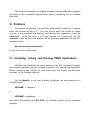
By providing a directory structure and template files, PGMT provides a
framework for building programs consistent with the PGM specification. To build
an application called AppName the user creates a directory with that name in the
directory ${PGM2_HOME}/apps
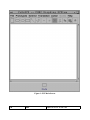
and populates the directory and its subdirectories with the files shown in Table 1. Templates of these files are provided
in the directories in ${PGM2_HOME}/apps/Template.
PGMT has been written
with the goal of allowing the user to develop programs with a minimum of
changes required to the files in the Template directory. As an aid to building PGMT
programs the apps directory contains five files ( Table 2) that are included in the
Makefiles of the AppName subdirectories. By using these files, the Makefiles of
Table 1 consist of only a few lines.
The CP subdirectory contains the command program and all associated
files. The Graph subdirectory contains the graph state files associated with the
File Name
Makefile
Appsrc
Makefile
CP
Makefile
CmdProg.cpp
CmdProg.h
Primitives
Makefile
external.h
Usage
Makefile for the overall build and linking
Parent directory of application source sub-directories
Makefile to build code in sub-directories
Command program sub-directory
Make file to build command program
C++ program defining CmdProg Class
C++ include file for CmdProg class
Subdirectory for c primitives
Makefile for building c primitives
Include file of c primitives signatures
t emplate_prim.c
Graph
Template.gsf
Makefile
MyList.h
template.h
Template of c primitive
Graph sub-directory
Sample gsf file
Make file to building C++ data type and Graph C++ class
Defines data types to be built
Defines the dataype C++ class.
Table 1: Files in Directory AppName
application as well as the files (if any) for user defined data types and the
translator produced C++ code. (Normally GSF files are created by the GUI - the
template is provided simply as an example.) The primitives subdirectory contains
the C code for any user supplied primitives. The role of the Makefiles and
directory structure for compiling and linking the PGMT executable is discussed in
Section VII.
IV. Writing Graphs
Data flow graphs are entered into the Processing Graph Method Tool via the
Java GUI. Building the graph consists of placing and connecting icons of the data
flow graph on the screen and filling out forms describing the icons and their
interconnections.
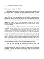
The steps to start the GUI depend on whether the user’s terminal is
connected directly to the computer running the GUI or the user is accessing a
remote host over a network. If the user is at a terminal connected directly to the
computer on which the GUI is running, the user merely changes to the directory
where he wants the graph state file to reside and types gui at the prompt. If the
user is accessing the GUI from a remote location, before starting the GUI, the
environmental variable DISPLAY must be set to the name of the local computer by
setenv DISPLAY hostname:0.0
and the local computer must allow the remote computer to open X windows on
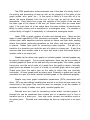
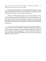
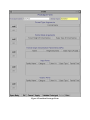
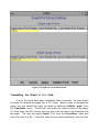
the local display. The window opened on the screen is shown in Figure 1. Across
the top of the screen is a set of menus available to the user. The user selects a
particular menu by using the mouse to move an arrow over the menu title and
clicking the left mouse button. Then the user moves the arrow over the desired
menu item and clicks the left mouse button to activate that selection.
summary of the menu actions is given in Table 2.
A
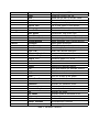
Below the menus should appear a tool bar that provides an easy way for the
user to interact with the graph. If the tool bar does not appear, it can be
displayed by selecting Show Tool Bar from the Action Menu. The toolbar provides
direct access to the entries under the Action and Node menus.
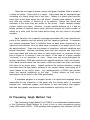
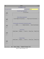
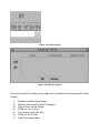
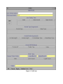
Much of the information about PGMT icons and links are entered via forms.
To the greatest extent possible, PGMT GUI forms have been developed to use
common features across the set of possible forms. Across the bottom of each
form (Figure 2) are buttons (Table 3) that are activated by clicking with the left
mouse button when the arrow is over the button. The buttons that are applicable
and active for a particular form are highlighted (usually all but the first button will
be highlighted).
Filling out some of the forms requires the construction of tables where the
number of rows in the table is application dependent. The addition and deletion of
rows to a table are performed by the use of the add and del buttons located on
the left hand side of the table. Initially tables to be constructed are empty and
rows are added by clicking the add button. To delete rows, the user moves the
arrow over an entry of the row and left clicks the mouse. The user then clicks the
del button to remove the row.
Figure 1. GUI Main Screen
File
New
Opens a file for a new GSF
Prototypes
Exterior
Translation
Action
Nodes
Help
Open
Close
Save
Save As
Preferences
Recent files
Exit
New OrdTran
New Queue
New GVar
Operator-defined
System-defined
Prototype
Banner
Port Association
Type List
Included Graph List
Validate Graph
Output C++
Undo
Clear
Delete
Cut
Copy
Paste
Print
Show Tool Bar
Select
Transition
Place
Included Graph
Arc
Arc Bends
Help
Release Notes
Known Problems
Version
Opens a previous GSF file
Closes the current GSF file
Saves the file with he current name
Saves the file in another directory
Changes some display values
List of files edited in this session
Leave the GUI
Construct new transition prototype
Construction new queue type
Construct new GVar prototype
Select prototype from operator defined
Select prototype from system-defined
Define graph prototype
Fill out the graph banner
Associate graph ports with node ports
Insert user defined datatypes
Insert included graphs
Verify graph is correct and complete
Construct graph C++ .h file
Undo last action
Returns to new state
Remove the selected feature
Copy and remove the selected feature
Copy the selected feature
Paste the last feature copied
Print out a copy of the graph
Toggle tool bar off and on
Go into select mode
Activate put transition mode
Activate put place mode
Activate put included graph
Activate arc mode
Activate mode to add bend in arc
On-line help
Revision history
Unimplemented Features
Date of last Update
Table 2: GUI Menu Contents
Figure 2 Graph Prototype form
Open body
OK
Cancel
Apply
Validate Graph
Print
Opens a new form for the C++ code of the icon
Applies and saves changes typed by user
Exits form making no changes since last save
Applies changes to form
Validates changes are consistent and complete
Prints a copy of the form
Table 3 : Common Action Buttons for Forms
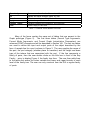
Many of the forms contain the same set of tables that are present in the
Graph prototype (Figure 2). The first three tables (Formal Type Arguments,
Formal Mode Arguments, and Formal Graph Instantiation Parameters) are
advanced PGMT concepts and will be described in Section VIII. The last two tables
are used to define the input and output ports of the object described by the
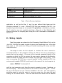
form. A sample line for a port is shown in Figure 3. The user supplies the name of
the port, the port category (whether place or transition) and the height and base
type of the tokens that are associated with the port. If the line represents a
family of ports, then the user double clicks on the little box in front of the Exp
Family… entry to display Figure 4, the family tree form. The user then adds lines
to the table and enters the index variable and lower and upper bounds of each
level of the family tree. The user can only construct from the GUI a regular family
of ports.
Figure 3 Port Description
Figure 4 Family Description
The entire process of entering the graph can be broken into several specific tasks,
namely
1)
2)
3)
4)
5)
6)
7)
Building and Saving the Graph
Defining User-specific Node Prototypes
Placing Icons on the Screen
Filling out Icon Forms
Connecting Icons with Arcs
Filling out Arc Forms
Graph Port Association
8)
Translating the Code to C++ code
Building and Saving the Graph
The first step in the building of a new graph is the selection of the New option
from the File menu. This opens a new empty graph with a prototype of New (or
Newn where n is a number if New.gsf, New0.gsf, … already exist). At any time
when no form is opened, Save from the File menu can be used to write the graph
state file graphname.gsf, where graphname is the graph prototype of the current
graph, to the disk. If the user desires to save the graph to a different directory,
the Save As selection f rom the File menu is used. The user moves through the
folders by double clicking on the file folder icon to move down through the
directory structure until the desired directory is reached and then clicking on the
save button to save the file. If the user desires to move up the directory
structure, he selects the appropriate directory from the menu available from the
box labeled Look in.
The next step is to define the prototype for the graph by selecting
Prototype from the Exterior menu. This will display the form previously shown
in Figure 2 . The user changes the prototype name from Newn to the name of the
graph and adds type arguments, mode arguments, GIPS, input ports, and output
ports as required. The user clicks on the add button to create an editable entry
for each of the items to be added and then fills in the contents of each row as
required. At any time the user can click on the Validate Prototype button t o
see if the entries are complete and correct. When the form is completed, the OK
button is clicked and, if valid, the form is saved and control returned to the iconic
graph. The GUI will not save an invalid form and returns control to the form if it
finds that the form is invalid. In the case of an invalid form, control may be
returned to the iconic GUI by using the cancel button. In this case, none of the
changes made to the form since the last successful Apply will be saved.
After the user completes the prototype form, the next form to be
completed is the banner form (Figure 5) under the Exterior menu. The first line
is read only and is automatically filled in by the GUI. The next three lines are
comments indicating the version of the graph, the author, and any appropriate
comments. Finally the user indicates if this is a main graph (the default) that will
be called by a command program, or an included graph that will be incorporated
into another graph.
If the user has created datatypes then the user includes the dataytype by
selecting the Type List entry from the Exterior menu to display the proper form.
Again, the add button is used to create a new entry line for each data type. In
each entry line, the datatype and name of the C++ file filename defining it are
entered as datatype@filename. The user can select the User defined Type entries
and click on the Browse button to display the contents of the datatype file.
If the user’s graph has included graph icons in it, then the prototypes of
these icons must be made available to the graph in order that links may be made
to the included graphs. This is accomplished in a similar manner to the process
for including user-defined datatypes. In this case the Included Graph List entry
in the Exterior menu is used to display the proper form. This form works the
same way as the Type List form
The only entry remaining for the graph exterior is the association of graph
data ports with ports in the graph. This function cannot be performed until the
ports of the icons in the graph have been defined. This cannot be done until step
5 is complete.
Defining User-specific Node Prototypes
The next step is to define the user written prototypes. To add a user defined prototype, the user selects New OrdTran, New Queue, or New GVar
from the Prototype menu. For a transition prototype, a form (Figure 9) similar to
the graph prototype is opened. In this case the entity type box will contain
transition and an Open Body button will be available on the form. The
Figure 5 Graph Banner
Figure 6 User Defined Types Form
Figure 7 Included Graph List
user fills in the form as was done for the graph prototype. In addition, a transition
performs operations on data. These operations are performed by the code in a
transition statement associated with the transition. These statements are entered
via the form (Figure 9) displayed by the Open Body button. The user may enter
the body by entering code into the window or reading the code from a file by use
of the read file button. The user will often have created the text for the
Figure 8 Transition Prototype Form
Figure 9 Transition Statement Form
transition statement in a separate file. (The editor in the GUI is limited in scope
and, by creating the transition statement outside of the GUI, the user has access
to any available editor -- ex, vi, emacs, xemacs, etc.
The user also may create special queue and graph variable place types. As
Figure 10 shows, these prototypes are more complex than the normal queue and
graph variable place types as they can have families of input and output ports.
They are much simpler than the transition prototypes as they have only one
family of input ports and one family of output ports and do not have transition
statements associated with them. Most applications will have user defined
transition prototypes, but will not use either of the special place types.
The user also has the option of deleting a prototype if for some reason it is
no longer needed by the graph. However the prototype cannot be deleted while
any node of the graph is currently using it.
Placing Icons on the Screen.
The user next places the icons (transitions, places, and/or included graphs) in
the graph screen window. The user first selects from the tool the type of icon
that is to be placed on the screen by clicking with the left mouse button the
corresponding icon on the tool bar. The arrow icon changes into a small dark icon
whose shape is the same as the icon to be placed on the screen. The user then
Figure 10 Place Prototype Form
moves the icon to the desired place on the screen and left clicks to place it on
the screen. This procedure is repeated until all of the icons for the graph are
placed on the screen. If a user wishes to delete an icon, the select icon (the left
most button on the toolbar) is chosen and the user left clicks on the icon to be
removed (the icon will turn red when it is selected) . The icon is removed by
clicking on the delete button (scissors) on the tool bar.
Once all of the tokens have been placed on the screen the user should return to
select mode by left clicking on the toolbar select button.
\ \
Filling out Icon forms
Next the user associates a prototype with each icon and fills out a form
describing the icon. While in select mode the user moves the arrow over the icon
and clicks the right mouse button. If the icon does not already have a prototype
associated with it, the set of allowable prototypes is presented as a menu. The
user uses the mouse to select one of these prototypes; the GUI then presents the
user with a choice of three forms to open: Call Form, Arc Form, or Prototype
Form). The latter two forms are read only and provide the user with descriptions
of the arcs connected to the icon and read access to the prototype form of the
icon. For the Call Form (Figure 12), the user must fill in the form describing the
icon. The user must first change the default name of the icon. A single icon may
represent a family of icons. If the icon does represent a family, then a description
of the family is provided in the area labeled Icon Family Tree.
The number of entry lines in the family table is the same as the height of
the family and the index variable and upper and lower bounds for each level of the
tree must be specified. If the prototype has type arguments, mode arguments
and/or associated GIPs, then the form will contain white boxes where the actual
values of these items must be entered.
If the icon is a transition or included graph then the bottom area of the
screen is inapplicable (as transitions and included graph do not have values) and
hence this area is inactive. For places, this area will be active. For a queue the
area may be filled with one or more tokens that will used to initialize the queue
when the graph is constructed. For a graph variable this area will be filled with
exactly one token that initializes the graph variable
The above procedures are repeated for each icon in the graph.
Connecting Icons with Directed Arcs
The user next connects the icons with directed arcs corresponding to the
flow of data within the graph. To connect two icons, the user first selects the arc
icon from the tool bar. The user then places the arrow over the icon providing
the data and drags it to the icon receiving the data and releases the mouse
button. A straight line will be drawn from the center of the first icon to the
center of the second icon with the line hidden when it passes through an icon.
Figure 11 Call Form
Each arc represents the connection of a port or family of ports on one icon
to a similar set on another icon.
At times the user may desire to draw more then one arc between the same
two icons or the arc drawn between two icons may be confusing or not
aesthetically pleasing. In this case, the user can put one or more bends in the arc.
To place a bend in an arc, the user selects Arc Bends from the tool bar, places
the arrow over a point on the line and drags with the left mouse button that point
to a new spot on the screen.
The point where the user releases the mouse
becomes the point for a bend with straight lines drawn from the two previous
ends of the line to the new point. By repeating this process the user may place
multiple bends in the same line. The right mouse button deletes bends.
Filling out Arc Forms
Now the user must define the endpoints for each arc. The user clicks on
the select button on the tool bar. For each arc between icons (whether straight
or bent) the user right clicks on the arc and selects the Arc Form entry (the only
choice) to display an Arc Form (Figure 12). The GUI checks to see what output
ports are available on the icons at the beginning of the directed arc and if there is
more than one port not currently connected, it presents the user with a menu for
choosing a port. If only one output port is available, the GUI automatically selects
it. Similarly the GUI checks the input ports on the icon at the end of the arc. The
GUI next displays the Arc Form.
Since a line can represent either a single arc or a family of arcs, the GUI
provides a table for defining a family of arcs when necessary. Again, the user uses
the add button to create the height of the arc family entry lines. Each arc is
between an output port (which may be a family) on one icon (which may also be a
family) and an input port (which may be a family) to an icon (which may be a
family). In the connect section of the form the user defines how these
connections take place. The GUI provides four lines in the connect section to
allow the user to define the connection with the families of ports and icons. The
user may also define a boolean condition that the connection is defined only on
the arcs for which the boolean evaluates to true. The default boolean is true (i.e.
all connections are made).
Figure 12 Arc Form
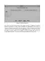
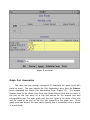
Graph Port Association
The user now has enough information to associate the graph ports with
ports on icons. The user selects the Port Association entry from the Exterior
menu displaying the Graph Port Association Form (Figure 13). The window
displays lines for the Graph Input Ports and Graph Output Ports with the name of
the port as the first entry on a line and entries for the aliased icon and
corresponding port. For each graph port, the user types in the name of the icon
and the name of the port on the icon that connects to the graph port. Since
graph ports are aliases, the user cannot specify that a connection be to a subset
of a port family.
Figure 13 Graph Port Associations Form
Translating the Graph to C++ Code
If all of the forms have been completely filled in correctly, the user should
be ready to translate the graph into a C++ class. Before trying to translate the
graph, the user should first verify the graph by selecting Validate graph from
the Translation menu. The GUI will now search for obvious errors in the graph.
If it finds none, the GUI informs the user that it did not detect any problems with
the graph. The user can select Output C++ from the Translation menu and
save the code to a file. If the GUI finds an error while translating, then the user
must go back and correct the error(s) and try again. All errors detected by the
GUI must be corrected before the C++ file can be created. While the GUI cannot
detect all errors, the GUI can verify that all required fields have been filled in, that
each port family is connected to another port family (except for the special
transitions where some of the ports are not required to be connected -- see Pack
and Unpack in the PGM specification), and that connected ports have the same
type.
At various points during the building of the graph the user can chose to exit
the GUI by selecting Exit from the File menu. If any changes have been made,
the GUI will ask if you want to save the graph before exiting. Usually, this
question should be answered by clicking on the OK button in which case the file is
saved before the GUI exits.
V. Writing Command Programs
The user writes the command program by developing the run method for
the CommandProgram class defined in CmdProg.cpp and CmdProg.h.
It is
through this method that the user controls what is happening in each of the
processes. While there is only one run method, the user can use the MPI rank, a
unique integer identifier that MPI provides for each process of the running
application, to determine what happens in each process at run time. In the run
method, the user constructs the graph, establishes communications between the
graph and the outside world, and controls the starting and stopping of the graph.
This method also contains all user-defined actions that are external to the graph.
For a graph that reads data from and writes data to its exterior, the user is
concerned with:
1)
2)
3)
4)
5)
6)
7)
8)
Defining the Process Type
Assigning Command Program Ports
Constructing the Graph
Attaching the Command Ports to the Graph
Starting the Graph
Writing Data to the Graph
Reading Data from the Graph
Stopping the Graph
An example of a simple run method for a graph that reads a vector of data and
produces a vector of data is given in Table 3.
void CommandProgram::run (int argc, char* argv[]) {
001
int i;
002
unsigned int outSize;
003
float in[32];
004
float *out;
005
vector< int > depth0;
006
cpRanks.push_back( 0);
007
for (int i=1; i<Machine::getNumProcesses(); i++) gRanks.push_back(i);
008
GraphPortAssignment portAssignment;
009
portAssignment.insert(GraphPortPair(GraphPortID("INPUT_GP",depth0),0));
010
portAssignment.insert(GraphPortPair(GraphPortID("OUTPUT_GP",depth0),0));
011
set_graph( new App(cpRanks,gRanks,portAssignment,(double) 1.0));
012
if (Machine::getCurrentProcessID() == 0 ){
013
GCL_GraphInport_T<float> *inputPort;
014
GCL_GraphOutport_T<float> *outputPort;
015
inputPort=(GCL_GraphInport_T<float>*)
get_graph()->getInPort( "INPUT_GP",depth0 );
016
outputPort=(GCL_GraphOutport_T<float>*)
get_graph()->getOutPort("OUTPUT_GP" ,depth0);
017
for (i=0; i<NELEM; i++){
in[i]=(float) 10.*drand48();
018
019
}
020
inputPort -> putVector(NELEM,*in);
021
while ( outputPort -> getContent() == 0 ) {}
022
out = outputPort -> getVector( outSize );
023
PGMT::stopGraph( *get_graph() );
024
else {
PGMT::startGraph( *get_graph() );
025
026
}
027
}
028
Defining the Process Type
The first action in the run method is the definition of the process type for
each process. Under the MPI model, each process has knowledge of the total
number of processes being run and the unique number between 0 and one less
than the number of processes that is associated with this process. (i. e. the MPI
rank).
The total number of processes is returned by a call to
Machine::getNumProcesses(),
while the unique numerical identifier of the
process is returned by Machine::getCurrentProcessID().
In PGMT the graph is
executed on a subset (that are referred to as the PEP processes) of the
processes. All of the other processes are referred to as non-PEP processes or
sometimes as command program processes. Data is written to and read from the
Graph by non-Pep processes. A copy of the graph must be resident on all
processes that reads data from or writes data to the graph. At the beginning of
the run method (see lines 007 and 008 in the example program) the user fills
the Standard Template Library (STL) vectors cpRanks with the process numbers
for the non-PEP processes communicating with the graph through graph ports and
gRanks with the process numbers of the PEP processes.
If the user had two non-PEP processes, with the first communicating with
the graph, the second not, and all the rest of the processes are PEP processes,
then the code could be
cpRanks.push_back( 0);
for (int i=2; i<Machine::getNumProcesses(); i++) gRanks.push_back(i);
In this case process 1 is not assigned to either the cpRank vector or the gRanks
vector.
Assigning Command Program Ports
The next step is to assign the graph ports of the main graph. On each of
the cpRanks and gRanks processes, the name, number and non-PEP process
that reads/writes through the graph port are inserted into a port assignment
table. The calling sequence to insert a single port is
portAssignment.insert(GraphPortPair(GraphPortID(p1,n1),n 2) ) ;
where p1 is the ASCII name of the port, n1 is the port number within the family,
and n2 is the process number of the non-PEP process that reads/writes the port.
Lines 008, 09, and 010 of the example run method assign the simple ports (i. e.
the graph port is really only a single port) defined by the ASCII strings INPUT_GP
and OUTPUT_GP.
The situation is more complicated if the graph port is actually a family of
individual ports. In this case, each individual port of the family must be inserted
into the table. If INPUT is a height 3 family of ports, with a 2x4x8 3-dimensional
matrix structure then the code to assign ports could be
if (isInCPRanksVector || isInCPRanksVector) {
int I,j,k;
vector <int> depth[3];
GraphPortAssignment portAssignment;
for (i=0; i<2;i++) {
for (j=0; j<4;j++) {
for (k=0; k<8, k++) {
depth[0]=i;
depth[1]=j;
depth[2]=k;
portAssignment.insert(GraphPortPair(GraphPortID
(“INPUT”,depth0),1));
}
}
}
}
Constructing the Graph
The next step is to build the graph on all processes specified by cpRanks
and gRanks. This is the only step where the user needs to write command
program code that is external to the run method.
At the beginning of
CmdProg.cpp where files with a .h extension are included in the source code, the
user adds the line
#include "Graph/App.h"
where App.h is the name of the file containing the C++ code generated by the
GUI from the GSF file for the graph. The graph is then constructed ( line 012) on
each process for each of the cpRanks and gRanks processes by using the
set_graph Method.
Attaching Command Program Ports to the Graph
Next non-PEP processes that write data to and read data from the graph
attach to the ports the graph. The methods are slightly different depending on
whether or not the port is used for writing data to the graph or reading data from
the graph. In the case of ports that write data of type datatype to the graph,
(line 016 of the example) the code to attach a port to port number portno would
be
GCL_GraphInport_T<datatype> *inputdataPort;
inputdataPort = (GCL_GraphInport_T<typedata>
get_graph()->getInPort(portno);
* )
Similarly ports that read data from the graph ( line 017 of the example) are
attached only Inport is replaced by Outport and input by output. Thus the code
for an output port would look like
GCL_GraphInport_T<datatype> *outputdataPort;
outputdataPort = (GCL_GraphOutport_T<typedata>
* )
get_graph()->getOutPort(portno);
Starting the Graph
The next step is to start the graph. No transitions will execute until the
graph has been started. Under PGMT the graph must be started on every PEP
process and only on PEP processes. The graph is started by the code
PGMT::startGraph(
*get_graph()
);
In the example, startGraph is called on line 26 and since it invoked in the else
block is only called by PEP processes. Control is not returned on these processes
to the command program run method until the graph is stopped.
Writing Data to the Graph
Data is written to a graph by using methods of the GCL_GraphInPort_T
class to construct and write a token to a place in the graph. The user must first
create a workspace to hold the token using the member function getWorkSpace
that returns a pointer to the workspace. The user then constructs the desired
token in the workspace and then uses the putToken member function to write the
token. The function putToken returns true if the token is successfully written to
the port (i. e. the token is put on the place to which the port is connected) and
false if not. Code to write data to a port could look like
datatype * in;
Boolean retVal;
in = inputdataPort -> getWorkSpace;
… code to build the token…
retVal=inputdataPort -> putToken();
Since constructing tokens from scratch is a complicated process, three special put
methods are available for writing to the graph: putLeaf for scalar, putVector for a
vector (a height 1 family), and putMatrix for a matrix of values (regular family
height 2). Examples of the code for each case (line 21 in the example code is for
the vector case), where inputdataPort has been declared as the type
GCL_GraphInport_T<datatype> and has already been attached to the command
program are
For a scalar :
bool retval;
datatype in;
in =xxxi;
retVal=inputdataPort -> putLeaf( in);
for a vector:
unsigned int i;
bool retval;
datatype in[1000];
for ( i=0; i < size; i++) in[i]==xxxi;
retVal=inputdataPort -> putVector( SIZE, in);
and for a matrix
unsigned int i,j,nrows=2--,ncols=300;
bool retval;
datatype in[100*200];
for ( i=0; i < size; i++) {
for (j=0;j< 300; j++) {
in[i*300+j]=xxxij;
}
}
retVal=inputdataPort -> putMatrix( 200,300, in);
where nrows and ncols are the number of rows and columns of the matrix
One of the reasons that a put operation may fail is that that the port is
attached to a queue that is at its capacity. To prevent this the user should use
the getCapacity method of the inputdataPort to ensure that the place attached
to the graph has sufficient capacity to write the token written to it. If there is not
sufficient capacity available, the user could then wait until the place has space
available by using the code
while ( inputdataPort
-> getCapacity()
== 0) { }
or using the code
if ( inputdataPort -> getCapacity()
code to write to the port
}
> 0) {
to write to the port only if the available capacity is greater than 0 and otherwise
to take other actions in his program and come back later to determine if he can
now write to the place.
At times the user may want to allow tokens to build up on an input queue
beyond that allowed by the capacity of the queue (this is automatically set by the
PEP and cannot be modified by the user). This capability is provided through the
use of force methods (forceToken, forceLeaf, forceVector and forceMatrix) that
will write to the queue even is the queue is at or over capacity. If the user does
this in an unconstrained way then tokens could conceivably build up without limit
on the input queue and eventually exhaust all of the memory available to the
program. To prevent this, the user can throttle the input by using the getContent
method to control the writing of data to the port. For example, the user could
use the code
while ( inputPort->getContent >10) {}
to wait until the current content of the input place is less than 10 before writing
to the port.
Reading Data from the Graph
Reading data from the graph is quit similar to writing data only instead of a
put, the program does a get and before trying to read a token the program call
getContent() is made to ensure there is a token on the port before doing the read
(line 022 of the example). As before the program can either go into a loop
waiting for a token to be on the place the port is hooked to by using the code
while ( outputdataPort -> getContent()
== 0 ) { }
or it may use an if like
if ( outputdataPort -> getContent()
code
}
!= 0 ) {
that will execute the c o d e
block only if there is a token on the port.
Corresponding to the equivalent puts we have get token getToken, getLeaf,
getVector, and getMatrix. Examples of the code for each case ( line 023 of the
example is for a vector), where outputdataPort has been declared as the type
GCL_GraphOutport_T<datatype> and already attached to the command program
are
for a general token:
GCL_WorkSpace_T<datatype> * out
out=outputdataPort -> getToken();
for a scalar :
datatype in;
in=inputdataPort -> getLeaf(;
for a vector:
unsigned int length;
datatype *out;
o u t=outputdataPort -> getVector( length) ;
where the starting address of the data is returned in out and the size of the
vector is returned in length.
and for a matrix:
unsigned int nrows,ncols;
datatype *out;
o u t=outputdataPort -> getMatrix(nrows,ncols);
where the starting address of the data is returned in out and the number of rows
and columns of the matrix are returned in nrows and ncols respectively.
Stopping the Graph
The final step is to stop the graph. In this case the command
PGMT::stopGraph(
*get_graph()
);
is executed on one (and only one) of the non-PEP processes containing a copy of
the graph ( line 024 of the example). It does not matter which of these
command process the command is issued on as long as only one process issues it.
This command stops the graphs running on the Pep processes and on the non-PEP
processes returns control from the PGMT startGraph method to the run method.
For example, the code
if (cpRanks[0] == Machine::getNumProcesses)
PGMT::stopGraph(*get_graph()
);
}
{
stops the graph with a command that is executed only from the first non-PEP
process that builds a graph.
The various processes now complete whatever user-specified work has been
specified by the command program writer before completing the run method
execution.
VI. Primitives
For reasons of efficiency, the transition statements of transitions in graphs
often call routines written in C. The user should place the source for these
routines in the primitives sub-directory and include their signatures in the file
external.h.
Note that even if the user includes no C primitives, this file
external.h must still be in the directory as the translator associated with the GUI
includes the line
#include<primitives/external.h>
in the .h file of the graph class.
VII. Compiling, Linking and Running PGMT Applications
After the user has written the codes outlined in the GUI, Command Program,
and primitives sections, the user is ready to compile, link, and run the application.
Before compiling and linking, the user must copy and modify the Makefiles
provided in the template directory.
For the Makefile in the root directory AppName, the user needs only to
change the line
APPNAME = Template
to
APPNAME = AppName
and add to the definition of LDFLAGS any libraries required by the command
program.
The Makefile's in appsrc and appsrc/CP do not need to be changed. The
Makefile in appsrc/primitives should have the line
SRC = template_prim.c
modified to compile the source code for the c primitives used in the graph. For
example, it the graph requires the c functions in s1.c, s2.c and s3.c, the line
should become
SRC= s1.c s2.c s3.c
After updating the makefiles as above, the user compiles, and runs the makefile in
the directory AppName. By simply typing the line
make
should build the desired command program. This process must be repeated for
each machine type.
The files run and machineFile are the files required to run the program under
MPICH.
The run file will contain one line of the form
mpirun -p4pg machineFile AppName.hostname
where AppName.hostname is the executable for the machine on which the run
command is executed..
The file machineFile will contain lines of the form
hostname 0 fullfilename
hostname 1 fullfilename
hostname 1 fullfilename
where the first line contains the name of the current host, a 0,
of the executable specified in the run command. The following
the name of a computer, a number specifying the number
executable to run on this computer, and the full filename of the
and the full name
lines each contain
of copies of the
executable.
The default run file provides the minimum required to run the command
program on the current host as PGMT requires as a minimum one non-PEP process
and two PEP processes. To run more processes, on the same or different hosts,
additional lines are added. More information on the format on the machineFile can
be found in the MPICH manual.
If the user is running on an HPC type machine, then the machineFile is not
needed and the run file will contain a file with the single line
mpirun -np n AppName.hostname
where n is the number of MPI processes to run.