Download User's Guide to AGMG

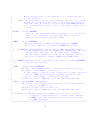
User’s Guide to AGMG
Yvan Notay
∗
Service de M´etrologie Nucl´eaire
Universit´e Libre de Bruxelles (C.P. 165/84)
50, Av. F.D. Roosevelt, B-1050 Brussels, Belgium.
email : [email protected]
February 2008
Revised: March 2009, March 2010, July 2011
January 2012, October 2012, March 2014
Abstract
This manual gives an introduction to the use of AGMG, a program which implements the algebraic multigrid method described in [Y. Notay, An aggregationbased algebraic multigrid method, Electronic Trans. Numer. Anal. (27: 123–146),
2010] with further improvements from [A. Napov and Y. Notay, An algebraic
multigrid method with guaranteed convergence rate, SIAM J. Sci. Comput., vol. 34,
pp. A1079-A1109, 2012] and from [Y. Notay, Aggregation-based algebraic multigrid
for convection-diffusion equations, SIAM J. Sci. Comput., vol. 34, pp. A2288-A2316,
2012].
This method solves algebraic systems of linear equations, and is expected to be
efficient for large systems arising from the discretization of scalar second order elliptic
PDEs. The method may however be tested on any problem, as long as all diagonal
entries of the system matrix are positive. It is indeed purely algebraic; that is, no
information has to be supplied besides the system matrix and the right-hand-side.
Both a sequential and a parallel FORTRAN 90 implementations are provided, as
well as an interface allowing to use the software as a Matlab function.
See the web site http://homepages.ulb.ac.be/~ynotay/AGMG for instructions
to obtain a copy of the software and possible updgrade.
Key words. FORTRAN, Matlab, multigrid, linear systems, iterative methods,
AMG, preconditioning, parallel computing, software.
AMS subject classification. 65F10
∗
Supported by the Belgian FNRS (“Directeur de recherches”)
! COPYRIGHT (c) 2012 Universite Libre de Bruxelles (ULB)
!
! ALL USAGE OF AGMG IS SUBJECT TO LICENSE. PLEASE REFER TO THE FILE "LICENSE".
! IF YOU OBTAINED A COPY OF THIS SOFTWARE WITHOUT THIS FILE,
! PLEASE CONTACT [email protected]
!
! In particular, if you have a free academic license:
!
! (1) You must be a member of an educational, academic or research institution.
!
The license agreement automatically terminates once you no longer fulfill
!
this requirement.
!
! (2) You are obliged to cite AGMG in any publication or report as:
!
"Yvan Notay, AGMG software and documentation;
!
see http://homepages.ulb.ac.be/~ynotay/AGMG".
!
! (3) You may not make available to others the software in any form, either
!
as source or as a precompiled object.
!
! (4) You may not use AGMG for the benefit of any third party or for any
!
commercial purposes. Note that this excludes the use within the
!
framework of a contract with an industrial partner.
!!!!!!!!!!!!!!!!!!!!!!!!!!!!!!!!!!!!!!!!!!!!!!!!!!!!!!!!!!!!!!!!!!!!!!!!!!
! DICLAIMER:
!
AGMG is provided on an "AS IS" basis, without any explicit or implied
!
WARRANTY; see the file "LICENSE" for more details.
!!!!!!!!!!!!!!!!!!!!!!!!!!!!!!!!!!!!!!!!!!!!!!!!!!!!!!!!!!!!!!!!!!!!!!!!!
!
If you use AGMG for research, please observe that your work benefits
!
our past research efforts that allowed the development of AGMG.
!
Hence, even if you do not see it directly, the results obtained thanks
!
to the use of AGMG depend on the results in publications [1-3] below,
!
where the main algorithms used in AGMG are presented and justified.
!
It is then a normal duty to cite these publications (besides citing
!
AGMG itself) in any scientific work depending on the usage of AGMG,
!
as you would do with any former research result you are using.
!
! [1] Y. Notay, An aggregation-based algebraic multigrid method,
!
Electronic Transactions on Numerical Analysis, vol. 37, pp. 123-146, 2010
!
! [2] A. Napov and Y. Notay, An algebraic multigrid method with guaranteed
!
convergence rate, SIAM J. Sci. Comput., vol. 34, pp. A1079-A1109, 2012.
!
! [3] Y. Notay, Aggregation-based algebraic multigrid for convection-diffusion
!
equations, SIAM J. Sci. Comput., vol. 34, pp. A2288-A2316, 2012.
2
Contents
1 Introduction
4
1.1
How to use this guide . . . . . . . . . . . . . . . . . . . . . . . . . . . . . .
4
1.2
Release notes . . . . . . . . . . . . . . . . . . . . . . . . . . . . . . . . . .
4
1.3
Installation and external libraries . . . . . . . . . . . . . . . . . . . . . . .
7
1.4
Error handling
. . . . . . . . . . . . . . . . . . . . . . . . . . . . . . . . .
8
1.5
Common errors . . . . . . . . . . . . . . . . . . . . . . . . . . . . . . . . .
8
2 Sequential version
9
2.1
Basic usage and matrix format . . . . . . . . . . . . . . . . . . . . . . . . .
9
2.2
Additional parameter . . . . . . . . . . . . . . . . . . . . . . . . . . . . . .
10
2.2.1
ijob . . . . . . . . . . . . . . . . . . . . . . . . . . . . . . . . . . .
10
2.2.2
iprint . . . . . . . . . . . . . . . . . . . . . . . . . . . . . . . . . .
11
2.2.3
nrest . . . . . . . . . . . . . . . . . . . . . . . . . . . . . . . . . .
11
2.2.4
iter . . . . . . . . . . . . . . . . . . . . . . . . . . . . . . . . . . .
11
2.2.5
tol . . . . . . . . . . . . . . . . . . . . . . . . . . . . . . . . . . . .
11
2.3
Example . . . . . . . . . . . . . . . . . . . . . . . . . . . . . . . . . . . . .
12
2.4
Printed output . . . . . . . . . . . . . . . . . . . . . . . . . . . . . . . . .
13
2.5
Fine tuning . . . . . . . . . . . . . . . . . . . . . . . . . . . . . . . . . . .
16
3 Parallel version
17
3.1
Basic usage and matrix format . . . . . . . . . . . . . . . . . . . . . . . . .
17
3.2
Example . . . . . . . . . . . . . . . . . . . . . . . . . . . . . . . . . . . . .
20
3.3
Printed output . . . . . . . . . . . . . . . . . . . . . . . . . . . . . . . . .
24
3.4
Tuning the parallel version . . . . . . . . . . . . . . . . . . . . . . . . . . .
26
4 Running several instances of AGMG
27
5 Solving singular systems
27
A Listing of DAGMG
29
B Listing of AGMGPAR
32
References
36
3
1
Introduction
The software package provides subroutines, written in FORTRAN 90, which implement
the method described in [7], with further improvements from [5, 8]. The main driver
subroutine is AGMG for the sequential version and AGMGPAR for the parallel version. Each
driver is available in double precision (prefix D), double complex (prefix Z), single precision
(prefix S) and single complex (prefix C) arithmetic. These subroutines are to be called from
an application program in which are defined the system matrix and the right-hand-side of
the linear system to be solved.
A Matlab interface is also provided; that is, an m-file (agmg.m) implementing a Matlab
function (agmg) that allows to call (sequential) AGMG from the Matlab environment.
This guide is directed towards the use of the FORTRAN version; however, Section 2.2 on
additional parameters, Section 2.4 on printed output and Sections 4–5 about some special
usages apply to the Matlab version as well. Basic information can also be obtained by
entering help agmg in the Matlab environment.
For a sample of performances in sequential and comparison with other solvers, see the paper
[6] and the report [9] (http://homepages.ulb.ac.be/~ynotay/AGMG/numcompsolv.pdf).
For performances of the parallel version, see [10].
1.1
How to use this guide
This guide is self contained, but does not describe methods and algorithms used in AGMG,
for which we refer to [7, 5, 8]. We strongly recommend their reading for an enlightened
use of the package.
On the other hand, main driver routines are reproduced in the Appendix with the comment
lines describing precisely each parameter. It is a good idea to have a look at the listing of
a driver routine while reading the section of this guide describing its usage.
1.2
Release notes
This guide describes AGMG 3.2.1-aca (academic version) and AGMG 3.2.1-pro (professional version).
New features from release 3.2.1:
• Improved treatment of singular systems; see Section 5.
4
• Professional version only. Improved parallel performance (verified weak scalability up
to 370,000 cores [10]).
• Professional version only. Compilation with the (provided) sequential MUMPS module can be replaced by a link with the Intel Math Kernel Library (MKL); see Section 1.3.
New features from release 3.2.0:
• Professional version only. A variant of the parallel version is provided that does
not require the installation of the parallel MUMPS library. See Section 1.3 and the
README file for details.
• The smoother is now SOR with automatic estimation of the relaxation parameter
ω , instead of Gauss-Seidel (which corresponds to SOR with ω = 1). In many cases,
AGMG still uses ω = 1 as before, but this new feature provides additional robustness,
especially in non symmetric cases.
• Default parameters for the parallel version have been modified, to improve scalability
when using many processors. This may induce slight changes in the convergence, that
should however not affect overall performances.
• Some compilation issues raised by the most recent versions of gfortran and ifort
have been solved, as well as some compatibility issues with the latest releases of the
MUMPS library.
New features from release 3.1.2:
• The printed output has been slightly changed: the work (number of floating points
operations) is now reported in term of “work units per digit of accuracy”, see Section 2.4 for details.
New features from release 3.1.1:
• A few bugs that sometimes prevented the compilation have been fixed; the code (especially MUMPS relates routines) has been also cleaned to avoid superfluous warning
messages with some compilers.
• The parameters that control the aggregation are now automatically adapted in case
of too slow coarsening.
• Some limited coverage of singular systems is now provided, see Section 5.
5
New features from release 3.0 (the first three have no influence on the software usage):
• The aggregation algorithm is no longer the one described in [7]. It has been exchanged
for the one in [5] in the symmetric case and for the one in [8] for general nonsymmetric
matrices (Note that this is the user who tells if the problem is to be treated as a
symmetric one or not via the parameter nrest, see Section 2.2.3 below).
This is an “internal” change; i.e., it has no influence on the usage of the software. It
makes the solver more robust and faster on average. We can however not exclude that
in some cases AGMG 3.0 is significantly slower than previous versions. This may, in
particular, happen for problems that are outside the standard scope of application.
Feel free to contact the author if you have such an example. AGMG is an ongoing
project and pointing out weaknesses of the new aggregation scheme can stimulate
further progress.
• Another internal change is that the systems on the coarsest grid are now solved
with the (sequential) MUMPS sparse direct solver [4]. Formerly, MUMPS was only
used with the parallel version. Using it also in the sequential case allows to improve
robustness; i.e. improved performances on “difficult” problems.
The MUMPS library needs however not be installed when using the sequential version. We indeed provide an additional source file that contains needed subroutines
from the MUMPS library. See Section 1.3 and the README file for details.
• The meaning of parameter nrest is slightly changed, as it influences also the aggregation process (see above). The rule however remains that nrest should be set to 1
only if the system matrix is symmetric positive definite; see Section 2.2.3 for details.
• It is now possible to solve a system with the transpose of the input matrix. This
corresponds to further allowed values for parameter ijob; see Section 2.2.1 below for
details.
• The meaning of the input matrix when using ijob not equal to its default is also
changed; see Section 2.2.1 below for details.
• The naming schemes and the calling sequence of each driver routine remain unchanged from releases 2.x, but there are slight differences with respect to releases
1.x. Whereas with releases 2.x routines were provided for backward compatibility,
these are no longer supported; i.e. application programs based on the naming scheme
and calling sequence of releases 1.x need to be adapted to the new scheme.
6
1.3
Installation and external libraries
AGMG does not need to be installed as a library. For the sake of simplicity, source files are
provided, and it is intended that they are compiled together with the application program
in which AGMG routines are referenced. See the README file provided with the package
for additional details and example of use.
AGMG requires LAPACK [1] and BLAS libraries. Most compilers come with an optimized
implementation of these libraries, and it is strongly recommended to use it. If not available, we provide needed routines from LAPACK and BLAS together with the package.
Alternatively LAPACK may be downloaded from http://www.netlib.org/lapack/ and
BLAS may be downloaded from http://www.netlib.org/blas/
Note that these software are free of use, but copyrighted. It is required the following. If
you modify the source for a routine we ask that you change the name of the routine and
comment the changes made to the original. This, of course, applies to the routines we
redistribute together with AGMG.
In addition, the parallel version requires the installation of the parallel MUMPS library
[4], which is also public domain and may be downloaded from http://graal.ens-lyon.
fr/MUMPS/.
Professional version only. The parallel MUMPS library needs not to be installed when using
the variant provided in the source files whose name contains “NM” (for “No MUMPS”;
see the README file for details). Indeed, this variant uses only a sequential version of
MUMPS, actually the same that is used by the sequential version of AGMG. Hence what is
written below for sequential AGMG applies verbatim to this variant of the parallel version.
Note that the performances of both variants may differ. As a general rule, the “MUMPSfree” variant is expected to be better, and even much better above 1000 cores [10]. Feel free
to contact us for advice if you seemingly face scalability issues with that version.
Despite the sequential version of AGMG also uses MUMPS, it does not require MUMPS
to be installed as a library. Actually, in the sequential case, AGMG requires only a subset
of MUMPS, and, for users’ convenience, files (one for each arithmetic) gathering needed
routines are provided together with AGMG. This is possible because MUMPS is public
domain; see the files header for detailed copyright notice. Note that all MUMPS routines
we provide with AGMG have been renamed (the prefixes d , s , . . . , have been exchanged
for dagmg , sagmg , . . . ). Hence you may use them in an application program that is also
linked with the MUMPS library: there will be no mismatch; in particular, no mismatch
between the sequential version we provide and the parallel version of MUMPS installed
by default. On the other hand, it means that if you have the sequential MUMPS library
installed and that you would like to use it instead of the version we provide, you need to
edit the source file of AGMG and restore the classical calling sequence to MUMPS.
7
Professional version only. When using the Intel compiler and linking with the Intel Math
Kernel Library (MKL), the provided subset of MUMPS can be skipped, because needed functionalities are retrieved from the MKL (using an appropriate flag when compiling AGMG;
see the README file for details).
1.4
Error handling
Except the case of a number of allowed iterations insufficient to achieve the convergence
criterion, any detected error is fatal and leads to a STOP statement, with a printed information that should allow to figure out what happened. Note that AGMG does not check
the validity of all input parameters. For instance, all diagonal entries of the supplied
matrix must be positive, but no explicit test is implemented. Feel free to contact the
author for further explanations if errors persist after checking that the input parameters
have been correctly defined.
1.5
Common errors
Be careful that iter and, in the parallel case, ifirstlistrank are also output parameters.
Hence declaring them as a constant in the calling program entails a fatal error.
Also, don’t forget to reinitialize iter between successive calls to AGMG or AGMGPAR.
8
2
2.1
Sequential version
Basic usage and matrix format
The application program has to call the main driver AGMG as follows.
1
call dagmg ( N , a , ja , ia , f , x , ijob , iprint , nrest , iter , tol )
N is the order of the linear system, whose matrix is given in arrays a , ja , ia . The right
hand side must be supplied in array f on input, and the computed solution is returned in
x on output; optionally, x may contain an initial guess on input, see Section 2.2.1 below.
The required matrix format is the “compressed sparse row” (CSR) format described, e.g.,
in [12]. With this format, nonzero matrix entries (numerical values) are stored row-wise in
a , whereas ja carries the corresponding column indices; entries in ia indicate then where
every row starts. That is, nonzero entries (numerical values) and column indices of row i
are located in a(k) , ja(k) for k =ia(i), . . . ,ia(i+1)-1. ia must have length (at least) N+1,
and ia(N+1) must be defined in such a way that the above rule also works for i =N; that
is, the last valid entry in arrays a , ja must correspond to index k =ia(N+1)-1.
By way of illustration, consider the matrix


10
−1
 −2 11

−3



−4 12
−5 
A=
 .


13
−8 −9
14
The compressed
vectors.
10.0
a =
1 4
ja =
1 3
ia =
sparse row format of A is given (non uniquely) by the following three
−1.0 −2.0 11.0 −3.0 −4.0 12.0 −5.0 13.0 14.0 −9.0 −8.0
1 2 4 2 3 5 4 5 3 2
6 9 10 13
As the example illustrates (see how is stored the last row of A), entries in a same row
may occur in any order. AGMG performs a partial reordering inside each row, so that, on
output, a and ja are possibly different than on input; they nevertheless still represent the
same matrix.
Note that the SPARSKIT package [11] (http://www-users.cs.umn.edu/~saad) contains
subroutines to convert various sparse matrix formats to CSR format.
9
2.2
Additional parameter
Other parameters to be supplied are ijob , iprint , nrest , iter and tol.
2.2.1
ijob
ijob has default value 0. With this value, the linear system will be solved in the usual
way with the zero vector as initial approximation; this implies a setup phase followed
by an iterative solution phase [7]. Non-default values allow to tell AGMG that an initial
approximation is given in x, and/or to call AGMG for setup only, for solve only, or for just
one application of the multigrid preconditioner (that is, a call to Algorithm 3.2 in [7] at
top level, to be exploited in a more complex fashion by the calling program).
ijob can also be used to tell AGMG to work with the transpose of the input matrix.
Details are as follows (see also comments in the subroutine listing in Appendix A).
ijob
0
10
1
2
12
3
-1
100,110,101,102,112
2,3,12,102,112
1,101
3
2,12,102,112
usage or remark
performs setup + solve + memory release, no initial guess
performs setup + solve + memory release, initial guess in x
performs setup only
(preprocessing: prepares all parameters for subsequent solves)
solves only (based on previous setup), no initial guess
solves only (based on previous setup), initial guess in x
the vector returned in x is not the solution of the linear system,
but the result of the action of the multigrid
preconditioner on the right hand side in f
erases the setup and releases internal memory
same as, respectively, 0,10,1,2,12 but
use the TRANSPOSE of the input matrix
require that one has previously called AGMG
with ijob=1 or ijob=101
the preconditioner defined when calling AGMG
is entirely kept in internal memory; hence:
the input matrix is not accessed
the input matrix is used only to perform matrix vector product
within the main iterative solution process
It means that, upon calls with ijob=2,12,102,112, the input matrix may differ from the
input matrix that was supplied upon the previous call with ijob=1 or IJOB ijob=101;
then AGMG attempts to solve a linear system with the “new” matrix using the preconditioner set up for the “old” one. The same remark applies to ijob≥ 100 or not: the
value ijob=1 or 101 determines whether the preconditioner set up and stored in internal
memory is based on the matrix or its transpose; the value ijob=2,12 or 102,112 is used
10
to determine whether the linear system to be solved is with the matrix or its transpose,
independently of the set up. Hence one may set up a preconditioner for a matrix and use
it for its transpose.
These functionalities (set up a preconditioner and use it for another matrix) are provided
for the sake of generality but should be used with care; in general, set up is fast with
AGMG and hence it is recommended to rerun it even if the matrix changes only slightly.
Matlab: the usage is the same except that one should not specify whether an initial
approximation is present in x . This is told via the presence or the absence of the argument.
Hence, for instance, ijob=0 gathers the functionality of both ijob=0 and ijob=10.
2.2.2
iprint
iprint is the unit number where information (and possible error) messages are to be
printed. A nonpositive number suppresses all messages, except the error messages which
will then be printed on standard output.
2.2.3
nrest
nrest is the restart parameter for GCR [2, 13] (an alternative implementation of GMRES
[12]), which is the default main iteration routine [7]. A nonpositive value is converted to
10 (suggested default).
If nrest=1, Flexible CG is used instead of GCR (when ijob=0,10,2, 12,100,110,102,112)
and also (ijob=0,1,100,101) some simplification are performed during the set up based on
the assumption that the input matrix is symmetric (there is then no more difference between ijob=1 and ijob=101). This is recommended if and only if the matrix is symmetric
and positive definite.
2.2.4
iter
iter is the maximal number of iterations on input, and the effective number of iterations
on output. Since it is both an input and an output parameter, it is important not to forget
to reinitialize it between successive call.
2.2.5
tol
tol is the tolerance on the relative residual norm; that is, iterations will be pursued (within
the allowed limit) until the residual norm is below tol times the norm of the input righthand-side.
11
2.3
Example
The source file of the following example is provided with the package.
Listing 1: source code of sequential Example
program example_seq
4
!
!
!
!
implicit none
real ( kind ( 0 d0 ) ) , allocatable : : a ( : ) , f ( : ) , x ( : )
integer , allocatable : : ja ( : ) , ia ( : )
integer : : n , iter , iprint , nhinv
real ( kind ( 0 d0 ) ) : : tol
9
!
!
14
!
!
!
!
19
!
!
24
29
34
S o l v e s t h e d i s c r e t e L a p l a c i a n on t h e u n i t s q u a r e by s i m p l e c a l l t o agmg .
The r i g h t −hand−s i d e i s such t h a t t h e e x a c t s o l u t i o n i s t h e v e c t o r o f a l l 1 .
!
!
!
!
!
!
!
!
!
!
!
s e t i n v e r s e o f t h e mesh s i z e ( f e e l f r e e t o change )
nhinv=500
maximal number o f i t e r a t i o n s
iter=50
t o l e r a n c e on r e l a t i v e r e s i d u a l norm
tol =1.e−6
u n i t number f o r o u t p u t messages : 6 => s t a n d a r d o u t p u t
iprint=6
g e n e r a t e t h e m a t r i x i n r e q u i r e d f o r m a t (CSR)
f i r s t a l l o c a t e the vectors with correct s i z e
N=(nhinv −1)∗∗2
allocate ( a ( 5 ∗ N ) , ja ( 5 ∗ N ) , ia ( N +1) , f ( N ) , x ( N ) )
next c a l l subroutine to set e n t r i e s
call uni2d ( nhinv −1,f , a , ja , ia )
c a l l agmg
argument 5 ( i j o b ) i s 0 b e c a u s e we want a c o m p l e t e s o l v e
argument 7 ( n r e s t ) i s 1 b e c a u s e we want t o use f l e x i b l e CG
( t h e m a t r i x i s symmetric p o s i t i v e d e f i n i t e )
call dagmg ( N , a , ja , ia , f , x , 0 , iprint , 1 , iter , tol )
!
39
END program example_seq
12
2.4
Printed output
The above example produces the following output.
****ENTERING AGMG *************************************************************
****
****
Number of unknowns:
Nonzeros :
249001
1243009 (per row:
4.99)
****SETUP: Coarsening by multiple pairwise aggregation
**** Rmk: Setup performed assuming the matrix symmetric
****
Quality threshold (BlockD): 8.00 ; Strong diag. dom. trs: 1.29
****
Maximal number of passes: 2 ; Target coarsening factor: 4.00
****
Threshold for rows with large pos. offdiag.: 0.45
****
****
****
Level:
Number of variables:
Nonzeros:
2
62000
(reduction ratio: 4.02)
309006 (per row: 5.0; red. ratio: 4.02)
****
****
****
Level:
Number of variables:
Nonzeros:
3
15375
(reduction ratio: 4.03)
76381 (per row: 5.0; red. ratio: 4.05)
****
****
****
Level:
Number of variables:
Nonzeros:
4
3721
(reduction ratio: 4.13)
18361 (per row: 4.9; red. ratio: 4.16)
****
****
****
****
Level:
Number of variables:
Nonzeros:
Exact factorization:
5
899
(reduction ratio: 4.14)
4377 (per row: 4.9; red. ratio: 4.19)
0.158 work units (*)
****
****
****
****
****
****
Grid
Operator
Theoretical Weighted
Effective Weighted
complexity:
complexity:
complexity:
complexity:
memory used (peak):
Setup time (Elapsed):
1.33
1.33
1.92 (K-cycle at each level)
1.92 (V-cycle enforced where needed)
2.54 real(8) words per nnz (
1.13E-01 seconds
24.11 Mb)
****SOLUTION: flexible conjugate gradient iterations (FCG(1))
****
AMG preconditioner with 1 Gauss-Seidel pre- and post-smoothing sweeps
****
at each level
13
****
****
****
****
****
****
****
****
****
****
****
****
****
****
****
****
****
****
Iter=
0
Resid=
Iter=
1
Resid=
Iter=
2
Resid=
Iter=
3
Resid=
Iter=
4
Resid=
Iter=
5
Resid=
Iter=
6
Resid=
Iter=
7
Resid=
Iter=
8
Resid=
Iter=
9
Resid=
Iter=
10
Resid=
- Convergence reached in
level 2
level 3
level 4
#call=
#call=
#call=
0.45E+02
0.14E+02
0.23E+01
0.87E+00
0.14E+00
0.35E-01
0.66E-02
0.23E-02
0.54E-03
0.13E-03
0.33E-04
10 iterations
10
20
40
Number of work units:
memory used for solution:
Solution time (Elapsed):
#cycle=
#cycle=
#cycle=
Relat.
Relat.
Relat.
Relat.
Relat.
Relat.
Relat.
Relat.
Relat.
Relat.
Relat.
-
20
40
80
res.=
res.=
res.=
res.=
res.=
res.=
res.=
res.=
res.=
res.=
res.=
mean=
mean=
mean=
0.10E+01
0.32E+00
0.51E-01
0.19E-01
0.31E-02
0.78E-03
0.15E-03
0.52E-04
0.12E-04
0.28E-05
0.74E-06
2.00
2.00
2.00
max=
max=
max=
2
2
2
11.89 per digit of accuracy (*)
3.33 real(8) words per nnz (
31.54 Mb)
2.55E-01 seconds
*** (*) 1 work unit represents the cost of 1 (fine grid) residual evaluation
****LEAVING AGMG * (MEMORY RELEASED) ******************************************
Note that each output line issued by the package starts with **** .
AGMG first indicates the size of the matrix and the number of nonzero entries. One then
enters the setup phase, and the name of the coarsening algorithm is recalled, together with
the basic parameters used. Note that these parameters need not be defined by the user:
AGMG always use default values. These, however, can be changed by expert users, see
Section 2.5 below.
The quality threshold is the threshold used to accept or not a tentative aggregate when applying the coarsening algorithms from [5, 8]; BlockD indicates that the algorithm from [5]
is used (quality for block diagonal smoother), whereas Jacobi is printed instead when the
algorithm from [8] is used (quality for Jacobi smoother). The strong diagonal dominance
threshold is the threshold used to keep outside aggregation rows and columns that are
strongly diagonally dominant; by default, it is set automatically according to the quality
threshold as indicated in [5, 8]. The maximal number of passes and the target coarsening
factor are the two remaining parameters described in these papers. In addition, nodes having large positive offdiagonal elements in their row or column are transferred unaggregated
to the coarse grid, and AGMG print the related threshold.
14
How the coarsening proceeds is then reported level by level. The matrix on last level is
factorized exactly, and the associated cost is reported in term of number of work units;
that is, AGMG reports the number of floating point operations needed for this factorization
divided by the number of floating point operations needed for one residual evaluation (at
top level: computation of b − A x for some b , x), which represents 1 work unit.
To summarize setup, AGMG then reports on “complexities”. The grid complexity is the
sum over all levels of the number of variables divided by the matrix size; the operator
complexity is the complexity relative to the number of nonzero entries; that is, it is the
sum over all levels of the number of nonzero entries divided by the number of nonzero entries
in the input matrix (see [7, eq. (4.1)]). The theoretical weighted complexity reflects the
cost of the preconditioner when two inner iterations are performed are each level; see [5,
page 15] (with γ = 2) for a precise definition. The effective weighted complexity corrects
the theoretical weighted complexity by taking into account that V-cycle is enforced at some
levels according to the strategy described in [7, Section 3]. This allows to better control
the complexity in cases where the coarsening is slow. In most cases, the coarsening is
fast enough and both weighted complexities will be equal, but, when they differ, only the
effective weighted complexity reflects the cost of the preconditioner as defined in AGMG.
Memory usage is reported in term of real*8 (double precision) words per nonzero entries in
the input matrix; the absolute value is also given in Mbyte. Note that AGMG reports the
peak memory; that is, the maximal amount used at any stage of the setup. This memory is
dynamically allocated within AGMG. Eventually, AGMG reports on the real time elapsed
during this setup phase.
Next one enters the solution phase. AGMG informs about the used iterative method (as
defined via input parameter nrest), the used smoother, and the number of smoothing steps
(which may also be tuned by expert users). How the convergence proceeds is then reported
iteration by iteration, with an indication of both the residual norm and the relative residual
norm (i.e., the residual norm divided by the norm of the right hand side). Note that values
reported for “Iter=0” correspond to initial values (nothing done yet). When the iterative
method is GCR, AGMG also reports on how many restarts have been performed.
Upon completion, AGMG reports, for each intermediate level, statistics about inner iterations; “#call” is the number of times one entered this level; “#cycle” is the cumulated
number of inner iterations; “mean” and “max” are, respectively, the average and the maximal number of inner iteration performed on each call. If V-cycle formulation is enforced
at some level (see [7, Section 3]), one will have #cycle=#call and mean=max=1.
Finally, the cost of this solution phase is reported, again in term of “work units”, but now
per digit of accuracy; that is, how many digit of accuracy have been gained is computed
as d = log10 (krk0 /krkf ) (where r0 and rf are respectively the initial and final residual
vectors), and the total number of work units for the solution phase is divided by d to
get the mean work needed per digit of accuracy. The code also reports the memory used
during this phase and the elapsed real time. Note that the report on memory usage does
15
not take into account the memory internally allocated within the sparse direct solver at
coarsest level (i.e., MUMPS).
2.5
Fine tuning
Some parameters referenced in [7, 5, 8] are assigned default values within the code, for the
sake of simplicity. However, expert users may tune these values, to improve performances
and/or if they experiment convergence problems. This can be done by editing the module
dagmg mem, at the top of the source file.
16
3
Parallel version
We assume that the previous section about the sequential version has been carefully read.
Many features are common between both versions, such as most input parameters and
the CSR matrix format (Section 2.1) and the meaning of output lines (Section 2.4). This
information will not be repeated here, where the focus is on the specific features of the
parallel version.
The parallel implementation has been developed to work with MPI and we assume that
the reader is somewhat familiar with this standard.
The parallel implementation is based on a partitioning of the rows of the system matrix,
and assumes that this partitioning has been applied before calling AGMGPAR. Thus, if
the matrix has been generated sequentially, some partitioning tool like METIS [3] should
be called before going to AGMGPAR.
The partitioning of the rows induces, inside AGMG, a partitioning of the variables. Part of
the local work is proportional to the number of nonzero entries in the local rows, and part
of it is proportional to the number of local variables (that is, the number of local rows).
The provided partitioning should therefore aim at a good load balancing of both these
quantities. Besides, the algorithm scalability (with respect to the number of processors)
will be best when minimizing the sum of absolute values of offdiagonal entries connecting
rows assigned to different processors (or tasks).
3.1
Basic usage and matrix format
To work, the parallel version needs that several instances of the application program have
been launched in parallel and have initialized a MPI framework, with a valid communicator.
Let MPI COMM be this communicator (by default, it is MPI COMM WORLD). All instances or
tasks sharing this MPI communicator must call simultaneously the main driver AGMGPAR
as follows.
1
call dagmgpar ( N , a , ja , ia , f , x , ijob , iprint , nrest , iter , tol
MPI_COMM , listrank , ifirstlistrank )
&
Each task should supply only a portion of the matrix rows in arrays a , ja , ia .
Each row should be referenced in one and only one task.
N is the number of local rows.
Local ordering. Local rows (and thus local variables) should have numbers 1, . . . , N .
If a global ordering is in use, a conversion routine should be called before AGMGPAR, see
the SPARSKIT package [11] (http://www-users.cs.umn.edu/~saad) for the handling
matrices in CSR format (for instance, extracting block of rows).
17
Nonlocal connections. Offdiagonal entries present in the local rows but connecting
with nonlocal variables are to be referenced in the usual way; however, the corresponding
column indices must be larger than N. The matrix supplied to AGMGPAR is thus formally
a rectangular matrix with N rows, and an entry Aij (with 1 ≤ i ≤ N) corresponds to a
local connection if j ≤ N and to an external connection if j > N .
Important restriction. The global matrix must be structurally symmetric
with respect to nonlocal connections. That is, if Aij corresponds to an external
connection, the local row corresponding to j , whatever the task to which it is assigned,
should also contain an offdiagonal entry (possibly zero) referencing (an external variable
corresponding to) i .
Consistency of local orderings. Besides the condition that they are larger than
N, indexes of nonlocal variable may be chosen arbitrarily, providing that their ordering is
consistent with the local ordering on their “home” task (the task to which the corresponding
row is assigned). That is, if Aij and Akl are both present and such that j , l > N , and if
further j and l have same home task (as specified in listrank, see below), then one should
have j < l if and only if, on their home task, the variable corresponding to j has lower
index than the variable corresponding to l .
These constraints on the input matrix should not be difficult to meet in practice. Thanks to
them, AGMG may set up the parallel solution process with minimal additional information.
In fact, AGMG has only to know what is the rank of the “home” task of each referenced
non-local variable. This information is supplied in input vector listrank.
Let jmin and jmax be, respectively, the smallest and the largest index of a non-local variable
referenced in ja (N < jmin ≤ jmax ). Only entries listrank(j) for jmin ≤ j ≤ jmax will be
referenced and need to be defined. If j is effectively present in ja, listrank(j) should
be equal to the rank of the “home” task of (the row corresponding to) j ; otherwise,
listrank(j) should be equal to an arbitrary nonpositive integer.
listrank is declared in AGMGPAR as listrank(ifirstlistrank:*).
Setting ifirstlistrank= jmin or ifirstlistrank=N+1 allows to save on memory, since
listrank(i) is never referenced for i < jmin (hence in particular for i ≤N ).
ijob : comments in Section 2.2.1 apply, except that the parallel version cannot work
directly with the transpose of the input matrix. Hence ijob=100,101,102,110,112 are not
permitted.
18
By way of illustration, consider the same matrix as in Section 2.1 partitioned into 3 tasks,
task 0 receiving rows 1 & 2, task 1 rows 3 & 4, and task 2 row 5. Firstly, one has to add a
few entries into the structure to enforce the structural symmetry with respect to non-local
connections:




−1
−1
10
10
 −2 11

 −2 11 0 −3 0 
−3




 → 
 .
−4
12
−5
−4
12
−5
A=







 0
13
0
13
−8 −9
14
−8 −9
14
Then A is given (non uniquely) by the following variables and vectors.
Task 0
n
a
ja
ia
listrank
=
=
=
=
=
2
10.0 −1.0 −2.0 11.0 −3.0 0.0 0.0
1 4 1 2 4 3 5
1 3 8
∗ ∗ 1 1 2
=
=
=
=
=
2
−4.0 12.0 −5.0 13.0 0.0 0.0
7 1 5 2 6 7
1 4 7
∗ ∗ ∗ ∗ 2 0 0
=
=
=
=
=
1
14.0 −9.0 −8.0
1 5 3
1 4
∗ ∗ 0 −1 1
Task 1
n
a
ja
ia
listrank
Task 2
n
a
ja
ia
listrank
Note that these vectors, in particular the numbering of nonlocal variables, were not constructed in a logical way, but rather to illustrate the flexibility and also the requirements
of the format. One sees for instance with Task 2 that the numbering of nonlocal variables
may be quite arbitrary as long as “holes” in listrank are filled with negative numbers.
19
3.2
Example
The source file of the following example is provided with the package. The matrix corresponding to the five-point approximation of the Laplacian on the unit square is partitioned
according a strip partitioning of the domain, with internal boundaries parallel to the x direction. Note that this strip partitioning is not optimal and has been chosen for the sake
of simplicity.
If IRANK> 0 , nodes at the bottom line have a non-local connection with task IRANK-1 , and
if IRANK<NPROC−1 , nodes at the top line have a non-local connection with task IRANK+1 .
Observe that these non-local variables are given indexes >N in subroutine uni2dstrip,
and that listrank is set up accordingly. Note also that with this simple example the
consistency of local orderings arises in a natural way.
Note also that each task will print its output in a different file. This is recommended.
Listing 2: source code of parallel Example
program example_par
3
!
!
!
!
!
!
implicit none
include ’mpif.h’
real ( kind ( 0 d0 ) ) , allocatable : : a ( : ) , f ( : ) , x ( : )
integer , allocatable : : ja ( : ) , ia ( : ) , listrank ( : )
integer : : n , iter , iprint , nhinv , NPROC , IRANK , mx , my , ifirstlistrank , ierr
real ( kind ( 0 d0 ) ) : : tol
character ∗10 filename
8
13
!
!
18
!
!
!
!
23
!
!
!
28
S o l v e s t h e d i s c r e t e L a p l a c i a n on t h e u n i t s q u a r e by s i m p l e c a l l t o agmg .
The r i g h t −hand−s i d e i s such t h a t t h e e x a c t s o l u t i o n i s t h e v e c t o r o f a l l 1 .
Uses a s t r i p p a r t i t i o n i n g o f t h e domain , w i t h i n t e r n a l b o u n d a r i e s p a r a l l e l
to the x direction .
s e t i n v e r s e o f t h e mesh s i z e ( f e e l f r e e t o change )
nhinv=1000
maximal number o f i t e r a t i o n s
iter=50
t o l e r a n c e on r e l a t i v e r e s i d u a l norm
tol =1.e−6
I n i t i a l i z e MPI
call MPI_INIT ( ierr )
call MPI_COMM_SIZE ( MPI_COMM_WORLD , NPROC , ierr )
call MPI_COMM_RANK ( MPI_COMM_WORLD , IRANK , ierr )
20
!
!
33
38
!
!
!
u n i t number f o r o u t p u t messages ( a l t e r n a t i v e : i p r i n t =10+IRANK)
iprint=10
filename ( 1 : 8 ) = ’res.out_ ’
write ( filename ( 9 : 1 0 ) , ’(i2 .2) ’ ) IRANK
! processor dependent
open ( iprint , file=filename , form=’formatted ’ )
calculate local grid size
mx=nhinv−1
my=(nhinv −1)/ NPROC
if ( IRANK < mod ( nhinv −1, NPROC ) ) my=my+1
43
48
53
58
!
!
!
!
!
!
!
!
!
!
!
!
!
!
!
!
f i r s t a l l o c a t e the vectors with correct s i z e
N=mx ∗my
allocate ( a ( 5 ∗ N ) , ja ( 5 ∗ N ) , ia ( N +1) , f ( N ) , x ( n ) , listrank ( 2 ∗ mx ) )
e x t e r n a l nodes c o n n e c t e d w i t h l o c a l ones on t o p and bottom
i n t e r n a l b o u n d a r i e s w i l l r e c e i v e numbers [N+ 1 , . . . ,N+2∗mx ]
ifirstlistrank=N+1
next c a l l subroutine to set e n t r i e s
b e f o r e , i n i t i a l i z e l i s t r a n k t o z e r o so t h a t e n t r i e s
t h a t do not c o r r e s p o n d t o a n o n l o c a l v a r i a b l e p r e s e n t
i n j a a r e anyway p r o p e r l y d e f i n e d
listrank ( 1 : 2 ∗ mx)=0
call uni2dstrip ( mx , my , f , a , ja , ia , IRANK , NPROC , listrank , ifirstlistrank )
c a l l agmg
argument 5 ( i j o b ) i s 0 b e c a u s e we want a c o m p l e t e s o l v e
argument 7 ( n r e s t ) i s 1 b e c a u s e we want t o use f l e x i b l e CG
( t h e m a t r i x i s symmetric p o s i t i v e d e f i n i t e )
call dagmgpar ( N , a , ja , ia , f , x , 0 , iprint , 1 , iter , tol ,
MPI_COMM_WORLD , listrank , ifirstlistrank )
63
68
g e n e r a t e t h e m a t r i x i n r e q u i r e d f o r m a t (CSR)
!
!
!
!
!
!
!
!
&
uncomment t h e f o l l o w i n g t o w r i t e s o l u t i o n on d i s k f o r c h e c k i n g
filename (1:8)= ’ s o l . out ’
w r i t e ( f i l e n a m e ( 9 : 1 0 ) , ’ ( i 2 . 2 ) ’ ) IRANK
open ( 1 1 , f i l e =f i l e n a m e , form =’ f o r m a t t e d ’ )
w r i t e ( 1 1 , ’ ( e22 . 1 5 ) ’ ) x ( 1 : n )
c l o s e (11)
73
END program example_par
21
! processor dependent
78
83
88
93
98
103
108
113
118
!−−−−−−−−−−−−−−−−−−−−−−−−−−−−−−−−−−−−−−−−−−−−−−−−−−−−−−−−−−−−−−−−−−−−−−
subroutine uni2dstrip ( mx , my , f , a , ja , ia , IRANK , NPROC , listrank , ifirstlistrank )
!
! F i l l a m a t r i x i n CSR f o r m a t c o r r e s p o n d i n g t o a c o n s t a n t c o e f f i c i e n t
! f i v e −p o i n t s t e n c i l on a r e c t a n g u l a r g r i d
! Bottom boundary i s an i n t e r n a l boundary i f IRANK > 0 , and
!
t o p boundary i s an i n t e r n a l boundary i f IRANK < NPROC−1
!
implicit none
real ( kind ( 0 d0 ) ) : : f ( ∗ ) , a ( ∗ )
integer : : mx , my , ia ( ∗ ) , ja ( ∗ ) , ifirstlistrank , listrank ( ifirstlistrank : ∗ )
integer : : IRANK , NPROC , k , l , i , j
real ( kind ( 0 d0 ) ) , parameter : : zero =0.0 d0 , cx=−1.0d0 , cy=−1.0d0 , cd =4.0 d0
!
k=0
l=0
ia (1)=1
do i=1,my
do j=1,mx
k=k+1
l=l+1
a ( l)=cd
ja ( l)=k
f ( k)=zero
if ( j < mx ) then
l=l+1
a ( l)=cx
ja ( l)=k+1
else
f ( k)=f ( k)−cx
end if
if ( i < my ) then
l=l+1
a ( l)=cy
ja ( l)=k+mx
else if ( IRANK == NPROC −1) then
f ( k)=f ( k)−cy
! r e a l boundary
else
l=l+1
! i n t e r n a l boundary ( t o p )
a ( l)=cy
! t h e s e e x t e r n a l nodes a r e g i v e n t h e
ja ( l)=k+mx
! numbers [ mx∗my + 1 , . . . , mx∗(my+1)]
listrank ( k+mx)=IRANK+1 ! Thus l i s t r a n k (mx∗my+1:mx∗(my+1))=IRANK+1
end if
if ( j > 1 ) then
l=l+1
22
123
128
133
138
143
a ( l)=cx
ja ( l)=k−1
else
f ( k)=f ( k)−cx
end if
if ( i > 1 ) then
l=l+1
a ( l)=cy
ja ( l)=k−mx
else if ( IRANK == 0 ) then
f ( k)=f ( k)−cy
! r e a l boundary
else
l=l+1
! i n t e r n a l boundary ( bottom )
a ( l)=cy
! t h e s e e x t e r n a l nodes a r e g i v e n t h e
ja ( l)=k+mx ∗ ( my+1)
! numbers [ mx∗(my+ 1 ) + 1 , . . . ,mx∗(my+2)]
listrank ( k+mx ∗ ( my+1))=IRANK−1
! Thus l i s t r a n k (mx∗(my+1)+1:mx∗(my+2))=IRANK−1
end if
ia ( k+1)=l+1
end do
end do
return
end subroutine uni2dstrip
23
3.3
Printed output
Running the above example with 4 tasks, task 0 produces the following output.
0*ENTERING AGMG *************************************************************
**** Global number of unknowns:
0*
Number of local rows:
**** Global number of nonzeros:
0*
Nonzeros in local rows:
998001
249750
4986009 (per row:
1247251 (per row:
5.00)
4.99)
0*SETUP: Coarsening by multiple pairwise aggregation
**** Rmk: Setup performed assuming the matrix symmetric
****
Quality threshold (BlockD): 8.00 ; Strong diag. dom. trs: 1.29
****
Maximal number of passes: 3 ; Target coarsening factor: 8.00
****
Threshold for rows with large pos. offdiag.: 0.45
0*
Level:
**** Global number of variables:
0*
Number of local rows:
**** Global number of nonzeros:
0*
Nonzeros in local rows:
2
124563
(reduction
31249
(reduction
622693 (per row: 5.0; red.
155996 (per row: 5.0; red.
ratio:
ratio:
ratio:
ratio:
8.01)
7.99)
8.01)
8.00)
0*
Level:
**** Global number of variables:
0*
Number of local rows:
**** Global number of nonzeros:
0*
Nonzeros in local rows:
3
15904
(reduction
3984
(reduction
80716 (per row: 5.1; red.
20135 (per row: 5.1; red.
ratio:
ratio:
ratio:
ratio:
7.83)
7.84)
7.71)
7.75)
0*
Level:
**** Global number of variables:
0*
Number of local rows:
**** Global number of nonzeros:
0*
Nonzeros in local rows:
0*
Exact factorization:
4
2034
(reduction
497
(reduction
10516 (per row: 5.2; red.
2513 (per row: 5.1; red.
0.123 work units (*)
ratio:
ratio:
ratio:
ratio:
7.82)
8.02)
7.68)
8.01)
****
****
0*
0*
****
****
Global grid
Global Operator
Local grid
Local Operator
Theoretical Weighted
Effective Weighted
complexity:
complexity:
complexity:
complexity:
complexity:
complexity:
24
1.14
1.14
1.14
1.14
1.33 (K-cycle at each level)
1.33 (V-cycle enforced where needed)
0*
0*
memory used (peak):
Setup time (Elapsed):
2.82 real(8) words per nnz (
1.27E+00 seconds
26.86 Mb)
0*SOLUTION: flexible conjugate gradient iterations (FCG(1))
****
AMG preconditioner with 1 Gauss-Seidel pre- and post-smoothing sweeps
****
at each level
**** Iter=
0
Resid= 0.63E+02
Relat. res.= 0.10E+01
**** Iter=
1
Resid= 0.20E+02
Relat. res.= 0.32E+00
**** Iter=
2
Resid= 0.54E+01
Relat. res.= 0.85E-01
**** Iter=
3
Resid= 0.20E+01
Relat. res.= 0.31E-01
**** Iter=
4
Resid= 0.53E+00
Relat. res.= 0.84E-02
**** Iter=
5
Resid= 0.30E+00
Relat. res.= 0.47E-02
**** Iter=
6
Resid= 0.81E-01
Relat. res.= 0.13E-02
**** Iter=
7
Resid= 0.37E-01
Relat. res.= 0.58E-03
**** Iter=
8
Resid= 0.10E-01
Relat. res.= 0.16E-03
**** Iter=
9
Resid= 0.36E-02
Relat. res.= 0.56E-04
**** Iter=
10
Resid= 0.15E-02
Relat. res.= 0.24E-04
**** Iter=
11
Resid= 0.53E-03
Relat. res.= 0.84E-05
**** Iter=
12
Resid= 0.21E-03
Relat. res.= 0.33E-05
**** Iter=
13
Resid= 0.84E-04
Relat. res.= 0.13E-05
**** Iter=
14
Resid= 0.29E-04
Relat. res.= 0.46E-06
**** - Convergence reached in
14 iterations ****
****
0*
0*
0*
level 2
level 3
#call=
#call=
14
28
Number of work units:
memory used for solution:
Solution time (Elapsed):
#cycle=
#cycle=
28
56
mean=
mean=
2.00
2.00
max=
max=
2
2
11.84 per digit of accuracy (*)
2.87 real(8) words per nnz (
27.35 Mb)
6.54E-01 seconds
0 (*) 1 work unit represents the cost of 1 (fine grid) residual evaluation
0*LEAVING AGMG * (MEMORY RELEASED) ******************************************
For some items, both a local and a global quantity are now given. All output lines starting
with **** correspond to global information and are printed only by the task with RANK
0. Other lines starts with xxx*, where “xxx” is the task RANK. They are printed by each
task, based on local computation. For instance, the work for the exact factorization at the
coarsest level is the local work as reported by MUMPS, divided by the number of local
floating point operations needed for one residual evaluation (to get the local number of
work units). On the other hand, the work for the solution phase is the number of local
floating point operations, again relative to the local cost of one residual evaluation. If one
has about the same number on each task, it means that the initial load balancing (whether
good or bad) has been well preserved in AGMG.
25
3.4
Tuning the parallel version
As already written in Section 2.5, default parameters defined in the module dagmgpar mem
at the very top of the source file are easy to change. Perhaps such tuning is more useful
in the parallel case than in the sequential one. Here performances not only depend on
the application, but also on the computer; e.g., the parameters providing smallest average
solution time may depend on the communication speed.
Compared with the sequential version, by default, the number of pairwise aggregation
passes npass has been increased from 2 to 3. This favors more aggressive coarsening, in
general at the price of some increase of the setup time. Hence, on average, this slightly
increases the sequential time of roughly 10 %. But this turns out to be often beneficial
in parallel, because this reduces the time spent on small grids where communications are
relatively more costly and more difficult to overlap with computation. If, however, you
experience convergence difficulties, it may be wise to restore the default npass=2. On
the other hand, you may try to obtain even more aggressive coarsening by increasing also
kaptg blocdia and/or kaptg dampJac, after having checked effects on the convergence
speed (they are application dependent).
Eventually, in the parallel case, it is worth checking how the solver works on the coarsest grid. Large set up time may indicate that this latter is too large. This can be reduced by decreasing maxcoarsesize and maxcoarsesizeslow. It is also possible to tune
their effect according to the number of processors in subroutine dagmgpar init (just below agmgpar mem). Conversely, increasing the size of the coarsest system may help reduce communications as long as the coarsest solver remains efficient, which depends not
only of this size, but also on the number of processors and on the communication speed.
Professional version only: with the variant “NM” that does not use the parallel MUMPS
library, the coarsest grid solver is a special iterative solver; parameters that define the target
accuracy and the maximal number of iterations at this level can also be tuned.
26
4
Running several instances of AGMG
In some contexts, it is interesting to have simultaneously in memory several instances of
the preconditioner. For instance, when a preconditioner for a matrix in block form is
defined considering separately the different blocks, and when one would like to use AGMG
for several of these blocks.
Such usage of AGMG is not foreseen with the present version. However, there is a simple
workaround. In the sequential case, copy the source file, say, dagmg.f90 to dagmg1.f90.
Then, edit dagmg1.f90, and make a global replacement of all instances of dagmg (lowercase)
by dagmg1, but not DAGMG_MUMSP (uppercase), which should remain unchanged. Repeat
this as many times as needed to generate dagmg2.f90, dagmg3.f90, etc. Then, compile
all these source files together with the application program and dagmg mumps.f90. The
application program can call dagmg1(), dagm2(), dagm3(), . . . , defining several instances
of the preconditioner that will not interact with each other.
You can proceed similarly with any arithmetic and also the parallel version. In the latter
case, replace all instances of dagmgpar by dagmgpar1 (no exception).
Matlab: the same result is obtained in an even simpler way. Copy the three files agmg.m,
dmtlagmg.mex??? and zmtlagmg.mex??? (where ??? depends upon your OS and architecture) to, say, agmg1.m, dmtlagmg1.mex??? and zmtlagmg1.mex???. Edit the m-file
agmg1.m, and replace the 3 calls to dmtlagmg by calls to dmtlagmg1 , and the 3 calls to
zmtlagmg by calls to zmtlagmg1 . Repeat this as many times as needed. Then, functions
agmg1, agmg2, . . . , are defined which can be called independently of each other.
5
Solving singular systems
Singular systems can be solved directly. Further, this is done automatically, without needing to tell the software that the provided system is singular. However, this usage should
be considered with care and a few limitations apply. Basically, it works smoothly when
the system is compatible and when the left null space is spanned by the vector of all ones
(i.e., the range of the input matrix is the set of vectors orthogonal to the constant vector
and the right hand side belongs to this set). Please note that failures in other cases are
generally not fatal and hence not detected if the solution is not checked appropriately; for
instance, AGMG may seemingly work well but returns a solution vector which is highly
dominated by null space components.
To handle such cases, note that AGMG can often be efficiently applied to solve the near
singular system obtained by deleting one row and one column in a linear system originally
singular (and compatible). This approach is not recommended in general because the
truncated system obtained in this way tends to be ill-conditioned and hence no very easy
27
to solve with iterative methods in general. However, it is sensible to use this approach with
AGMG because one of the features of the method in AGMG is precisely its capability to
solve efficiently ill-conditioned linear systems.
28
A
2
7
12
17
22
27
32
37
42
Listing of DAGMG
SUBROUTINE dagmg ( n , a , ja , ia , f , x , ijob , iprint , nrest , iter , tol )
INTEGER
: : n , ia ( n +1) , ja ( ∗ ) , ijob , iprint , nrest , iter
REAL ( kind ( 0 . 0 d0 ) ) : : a ( ∗ ) , f ( n ) , x ( n )
REAL ( kind ( 0 . 0 d0 ) ) : : tol
! !!!!!!!!!!!!!!!!!!!!!!!!!!!!!!!!!!!!!!!!!!!!!!!!!!!!!!!!!!!!!!!!!!!!!!!!!!!!
!
! Arguments
! =========
!
! N
( i n p u t ) INTEGER.
!
The dimension o f t h e m a t r i x .
!
! A
( i n p u t / o u t p u t ) REAL ( k i n d ( 0 . 0 e0 ) ) . Numerical v a l u e s o f t h e m a t r i x .
! IA
( i n p u t / o u t p u t ) INTEGER. P o i n t e r s f o r e v e r y row .
! JA
( i n p u t / o u t p u t ) INTEGER. Column i n d i c e s .
!
!
AGMG ASSUMES THAT ALL DIAGONAL ENTRIES ARE POSITIVE
!
!
D e t a i l e d d e s c r i p t i o n of the matrix format
!
!
On i n p u t , IA ( I ) , I = 1 , . . . ,N, r e f e r s t o t h e p h y s i c a l s t a r t
!
o f row I . That i s , t h e e n t r i e s o f row I a r e l o c a t e d
!
i n A(K) , where K=IA ( I ) , . . . , IA ( I +1)−1. JA(K) c a r r i e s t h e
!
a s s o c i a t e d column i n d i c e s . IA (N+1) must be d e f i n e d i n such
!
a way t h a t t h e a b ov e r u l e a l s o works f o r I=N ( t h a t i s ,
!
t h e l a s t v a l i d e n t r y i n a r r a y s A, JA s h o u l d c o r r e s p o n d t o
!
i n d e x K=IA (N+1) −1). According what i s w r i t t e n
!
above , AGMG assumes t h a t some o f t h e s e JA(K) ( f o r
!
IA ( I)<= K < IA ( I +1) ) i s e q u a l t o I w i t h c o r r e s p o n d i n g
!
A(K) c a r r y i n g t h e v a l u e o f t h e d i a g o n a l element ,
!
which must be p o s i t i v e .
!
!
A, IA , JA a r e ” o u t p u t ” p a r a m e t e r s b e c a u s e on e x i t t h e
!
e n t r i e s o f each row may o c c u r i n a d i f f e r e n t o r d e r ( The
!
m a t r i x i s m a t h e m a t i c a l l y t h e same , b u t s t o r e d i n
!
d i f f e r e n t way ) .
!
! F
( i n p u t / o u t p u t ) REAL ( k i n d ( 0 . 0 e0 ) ) .
!
On i n p u t , t h e r i g h t hand s i d e v e c t o r f .
!
O v e r w r i t t e n on o u t p u t .
!
S i g n i f i c a n t o n l y i f IJOB==0, 2 , 3 , 10 , 12 , 100 , 102 , 110 , 112
!
29
47
52
57
62
67
72
77
82
87
! X
( i n p u t / o u t p u t ) REAL ( k i n d ( 0 . 0 e0 ) ) .
!
On i n p u t and i f IJOB== 10 , 12 , 110 , 1 1 2 : i n i t i a l g u e s s
!
( f o r o t h e r v a l u e s o f IJOB , t h e d e f a u l t i s used : t h e z e r o v e c t o r ) .
!
On o u t p u t , t h e computed s o l u t i o n .
!
! IJOB
( i n p u t ) INTEGER. T e l l s AGMG what has t o be done .
!
0 : p e r f o r m s s e t u p + s o l v e + memory r e l e a s e , no i n i t i a l g u e s s
!
1 0 : p e r f o r m s s e t u p + s o l v e + memory r e l e a s e , i n i t i a l g u e s s i n x ( 1 : n )
!
1: performs setup only
!
( p re pr oc es si ng : prepares a l l parameters f o r subsequent s o l v e s )
!
2 : s o l v e s o n l y ( b a s e d on p r e v i o u s s e t u p ) , no i n i t i a l g u e s s
!
1 2 : s o l v e s o n l y ( b a s e d on p r e v i o u s s e t u p ) , i n i t i a l g u e s s i n x ( 1 : n )
!
3 : t h e v e c t o r r e t u r n e d i n x ( 1 : n ) i s not t h e s o l u t i o n o f t h e l i n e a r
!
system , b u t t h e r e s u l t o f t h e a c t i o n o f t h e m u l t i g r i d
!
p r e c o n d i t i o n e r on t h e r i g h t hand s i d e i n f ( 1 : n )
!
−1: e r a s e s t h e s e t u p and r e l e a s e s i n t e r n a l memory
!
!
IJOB == 1 0 0 , 1 1 0 , 1 0 1 , 1 0 2 , 1 1 2 : same as , r e s p e c t i v e l y , IJOB==0 ,10 ,1 ,2 ,12
!
but , use t h e TRANSPOSE o f t h e i n p u t m a t r i x i n A, JA , IA .
!
!
! ! ! IJOB==2 ,3 ,12 ,102 ,112 r e q u i r e t h a t one has p r e v i o u s l y c a l l e d AGMG
!
w i t h IJOB==1 or IJOB==101
!
!
! ! ! ( change w i t h r e s p e c t t o v e r s i o n s 2 . x ) ! ! !
!
The p r e c o n d i t i o n e r d e f i n e d when c a l l i n g AGMG
!
w i t h IJOB==1 or IJOB==101 i s e n t i r e l y k e p t i n i n t e r n a l memory .
!
Hence t h e a r r a y s A, JA and IA a r e not a c c e s s e d upon s u b s e q u e n t c a l l s
!
w i t h IJOB==3.
!
Upon s u b s e q u e n t c a l l s w i t h IJOB==2 ,12 ,102 ,112 , a m a t r i x n ee d s t o
!
be s u p p l i e d i n a r r a y s A, JA , IA , b u t i t w i l l be used t o
!
perform m a t r i x v e c t o r p r o d u c t w i t h i n t h e main i t e r a t i v e
!
s o l u t i o n p r o c e s s ( and o n l y f o r t h i s ) .
!
Hence t h e system i s s o l v e d w i t h t h i s m a t r i x which
!
may d i f f e r from t h e m a t r i x i n A, JA , IA t h a t was s u p p l i e d
!
upon t h e p r e v i o u s c a l l w i t h IJOB==1 or IJOB==101;
!
t h e n AGMG a t t e m p t s t o s o l v e a l i n e a r system w i t h t h e ”new”
!
m a t r i x ( s u p p l i e d when IJOB==2 ,12 ,102 or 112) u s i n g t h e
!
p r e c o n d i t i o n e r s e t up f o r t h e ” o l d ” one ( s u p p l i e d when
!
IJOB==1 or 1 0 1 ) .
!
The same remarks a p p l y t o IJOB >= 100 or not : t h e v a l u e IJOB==1
!
or 101 d e t e r m i n e s w h e t h e r t h e p r e c o n d i t i o n e r s e t up and s t o r e d
!
i n i n t e r n a l memory i s b a s e d on t h e m a t r i x or i t s t r a n s p o s e ;
!
t h e v a l u e IJOB==2,12 or 102 ,112 i s used t o d e t e r m i n e w h e t h e r
!
t h e l i n e a r system t o be s o l v e d i s w i t h t h e m a t r i x or i t s
!
t r a n s p o s e , i n d e p e n d e n t l y o f t h e s e t up .
30
92
97
102
107
112
117
122
127
132
!
!
!
!
!
!
!
!
!
!
!
!
!
!
!
!
!
!
!
!
!
!
!
!
!
!
!
!
!
!
!
!
!
!
!
!
!
!
!
!
!
!
!
!
!
Hence one may s e t up a p r e c o n d i t i o n e r f o r a m a t r i x and use i t
for i t s transpose .
These f u n c t i o n a l i t i e s ( s e t up a p r e c o n d i t i o n e r and use i t f o r a n o t h e r
m a t r i x ) a r e p r o v i d e d f o r t h e s a k e o f g e n e r a l i t y b u t s h o u l d be
used w i t h c a r e ; i n g e n e r a l , s e t up i s f a s t w i t h AGMG and hence
i t i s recommended t o re r un i t even i f t h e m a t r i x c h a n g e s o n l y
slightly .
IPRINT
( i n p u t ) INTEGER.
I n d i c a t e s t h e u n i t number where i n f o r m a t i o n i s t o be p r i n t e d
(N.B . : 5 i s c o n v e r t e d t o 6 ) . I f n o n p o s i t i v e , o n l y e r r o r
messages a r e p r i n t e d on s t a n d a r d o u t p u t .
NREST
( i n p u t ) INTEGER.
R e s t a r t parameter f o r GCR ( an i m p l e m e n t a t i o n o f GMRES)
N o n p o s i t i v e v a l u e s a r e c o n v e r t e d t o NREST=10 ( d e f a u l t )
!!
!!!
!!!
I f NREST==1, F l e x i b l e CG i s used i n s t e a d o f GCR ( when IJOB==0 ,10 ,2 ,
1 2 , 1 0 0 , 1 1 0 , 1 0 2 , 1 1 2 ) and a l s o ( IJOB==0 ,1 ,100 ,101) p e r f o r m s some
s i m p l i f i c a t i o n d u r i n g t h e s e t up b a s e d on t h e ass um pti on
t h a t t h e m a t r i x s u p p l i e d i n A, JA , IA i s symmetric ( t h e r e i s
t h e n no more d i f f e r e n c e b e t w e e n IJOB==1 and IJOB==101).
NREST=1 S h o u l d be used i f and o n l y i f t h e m a t r i x i s r e a l l y SYMMETRIC
( and p o s i t i v e d e f i n i t e ) .
ITER
( i n p u t / o u t p u t ) INTEGER.
On i n p u t , t h e maximum number o f i t e r a t i o n s . S h o u l d be p o s i t i v e .
On o u t p u t , a c t u a l number o f i t e r a t i o n s .
I f t h i s number o f i t e r a t i o n was i n s u f f i c i e n t t o meet c o n v e r g e n c e
c r i t e r i o n , ITER w i l l be r e t u r n e d n e g a t i v e and e q u a l t o t h e
o p p o s i t e o f t h e number o f i t e r a t i o n s performed .
S i g n i f i c a n t o n l y i f IJOB==0, 2 , 10 , 12 , 100 , 102 , 110 , 112
TOL
( i n p u t ) REAL ( k i n d ( 0 . 0 e0 ) ) .
The t o l e r a n c e on r e s i d u a l norm . I t e r a t i o n s a r e s t o p p e d whenever
| | A∗x−f | | <= TOL∗ | | f | |
S h o u l d be p o s i t i v e and l e s s than 1 . 0
S i g n i f i c a n t o n l y i f IJOB==0, 2 , 10 , 12 , 100 , 102 , 110 , 112
! ! ! ! Remark ! ! ! ! E xcept i n s u f f i c i e n t number o f i t e r a t i o n s t o a c h i e v e
c o n v e r g e n c e ( c h a r a c t e r i z e d by a n e g a t i v e v a l u e r e t u r n e d
i n ITER) , a l l o t h e r d e t e c t e d e r r o r s a r e f a t a l and l e a d
t o a STOP s t a t e m e n t .
!!!!!!!!!!!!!!!!!!!!!!!!!!!!!!!!!!!!!!!!!!!!!!!!!!!!!!!!!!!!!!!!!!!!!!!!!!!!
31
B
135
140
145
150
155
160
165
170
175
Listing of AGMGPAR
SUBROUTINE dagmgpar ( n , a , ja , ia , f , x , ijob , iprint , nrest , iter , tol &
, MPI_COMM_AGMG , listrank , ifirstlistrank )
INTEGER
: : n , ia ( n +1) , ja ( ∗ ) , ijob , iprint , nrest , iter
REAL ( kind ( 0 . 0 d0 ) ) : : a ( ∗ ) , f ( n ) , x ( n )
REAL ( kind ( 0 . 0 d0 ) ) : : tol
INTEGER
: : MPI_COMM_AGMG , ifirstlistrank , listrank ( ∗ )
!
Actually : listrank ( i f i r s t l i s t r a n k :∗)
!
− l i s t r a n k i s o n l y used i n l o w e r l e v e l s u b r o u t i n e s
! !!!!!!!!!!!!!!!!!!!!!!!!!!!!!!!!!!!!!!!!!!!!!!!!!!!!!!!!!!!!!!!!!!!!!!!!!!!!
!
! Arguments
! =========
!
! N
( i n p u t ) INTEGER.
!
The dimension o f t h e m a t r i x .
!
! A
( i n p u t / o u t p u t ) REAL ( k i n d ( 0 . 0 e0 ) ) . Numerical v a l u e s o f t h e m a t r i x .
! IA
( i n p u t / o u t p u t ) INTEGER. P o i n t e r s f o r e v e r y row .
! JA
( i n p u t / o u t p u t ) INTEGER. Column i n d i c e s .
!
!
AGMG ASSUMES THAT ALL DIAGONAL ENTRIES ARE POSITIVE
!
!
D e t a i l e d d e s c r i p t i o n of the matrix format
!
!
On i n p u t , IA ( I ) , I = 1 , . . . ,N, r e f e r s t o t h e p h y s i c a l s t a r t
!
o f row I . That i s , t h e e n t r i e s o f row I a r e l o c a t e d
!
i n A(K) , where K=IA ( I ) , . . . , IA ( I +1)−1. JA(K) c a r r i e s t h e
!
a s s o c i a t e d column i n d i c e s . IA (N+1) must be d e f i n e d i n such
!
a way t h a t t h e a b ov e r u l e a l s o works f o r I=N ( t h a t i s ,
!
t h e l a s t v a l i d e n t r y i n a r r a y s A, JA s h o u l d c o r r e s p o n d t o
!
i n d e x K=IA (N+1) −1). According what i s w r i t t e n
!
above , AGMG assumes t h a t some o f t h e s e JA(K) ( f o r
!
IA ( I)<= K < IA ( I +1) ) i s e q u a l t o I w i t h c o r r e s p o n d i n g
!
A(K) c a r r y i n g t h e v a l u e o f t h e d i a g o n a l element ,
!
which must be p o s i t i v e .
!
!
A, IA , JA a r e ” o u t p u t ” p a r a m e t e r s b e c a u s e on e x i t t h e
!
e n t r i e s o f each row may o c c u r i n a d i f f e r e n t o r d e r ( The
!
m a t r i x i s m a t h e m a t i c a l l y t h e same , b u t s t o r e d i n
!
d i f f e r e n t way ) .
!
! F
( i n p u t / o u t p u t ) REAL ( k i n d ( 0 . 0 e0 ) ) .
!
On i n p u t , t h e r i g h t hand s i d e v e c t o r f .
32
180
185
190
195
200
205
210
215
220
!
O v e r w r i t t e n on o u t p u t .
!
S i g n i f i c a n t o n l y i f IJOB==0, 2 , 3 , 10 or 12
!
! X
( i n p u t / o u t p u t ) REAL ( k i n d ( 0 . 0 e0 ) ) .
!
On i n p u t and i f IJOB==10 or IJOB==12, i n i t i a l g u e s s
!
( f o r o t h e r v a l u e s o f IJOB , t h e d e f a u l t i s used : t h e z e r o v e c t o r ) .
!
On o u t p u t , t h e computed s o l u t i o n .
!
! IJOB
( i n p u t ) INTEGER. T e l l s AGMG what has t o be done .
!
0 : p e r f o r m s s e t u p + s o l v e + memory r e l e a s e , no i n i t i a l g u e s s
!
1 0 : p e r f o r m s s e t u p + s o l v e + memory r e l e a s e , i n i t i a l g u e s s i n x ( 1 : n )
!
1: performs setup only
!
( p re pr oc es si ng : prepares a l l parameters f o r subsequent s o l v e s )
!
2 : s o l v e s o n l y ( b a s e d on p r e v i o u s s e t u p ) , no i n i t i a l g u e s s
!
1 2 : s o l v e s o n l y ( b a s e d on p r e v i o u s s e t u p ) , i n i t i a l g u e s s i n x ( 1 : n )
!
3 : t h e v e c t o r r e t u r n e d i n x ( 1 : n ) i s not t h e s o l u t i o n o f t h e l i n e a r
!
system , b u t t h e r e s u l t o f t h e a c t i o n o f t h e m u l t i g r i d
!
p r e c o n d i t i o n e r on t h e r i g h t hand s i d e i n f ( 1 : n )
!
−1: e r a s e s t h e s e t u p and r e l e a s e s i n t e r n a l memory
!
!
! ! ! IJOB==2 ,3 ,12 r e q u i r e t h a t one has p r e v i o u s l y c a l l e d AGMG w i t h IJOB==1
!
!
! ! ! ( change w i t h r e s p e c t t o v e r s i o n s 2 . x ) ! ! !
!
The p r e c o n d i t i o n e r d e f i n e d when c a l l i n g AGMG
!
w i t h IJOB==1 i s e n t i r e l y k e p t i n i n t e r n a l memory .
!
Hence t h e a r r a y s A, JA and IA a r e not a c c e s s e d upon s u b s e q u e n t c a l l s
!
w i t h IJOB==3.
!
Upon s u b s e q u e n t c a l l s w i t h IJOB==2, 12 , a m a t r i x n ee d s t o
!
be s u p p l i e d i n a r r a y s A, JA , IA , b u t i t w i l l be used t o
!
perform m a t r i x v e c t o r p r o d u c t w i t h i n t h e main i t e r a t i v e
!
s o l u t i o n p r o c e s s ( and o n l y f o r t h i s ) .
!
Hence t h e system i s s o l v e d w i t h t h i s m a t r i x which
!
may d i f f e r from t h e m a t r i x i n A, JA , IA t h a t was s u p p l i e d
!
upon t h e p r e v i o u s c a l l w i t h IJOB==1;
!
t h e n AGMG a t t e m p t s t o s o l v e a l i n e a r system w i t h t h e ”new”
!
m a t r i x ( s u p p l i e d when IJOB==2,12) u s i n g t h e p r e c o n d i t i o n e r
!
s e t up f o r t h e ” o l d ” one ( s u p p l i e d when IJOB==1).
!
These f u n c t i o n a l i t i e s ( s e t up a p r e c o n d i t i o n e r and use i t f o r a n o t h e r
!
m a t r i x ) a r e p r o v i d e d f o r t h e s a k e o f g e n e r a l i t y b u t s h o u l d be
!
used w i t h c a r e ; i n g e n e r a l , s e t up i s f a s t w i t h AGMG and hence
!
i t i s recommended t o re r un i t even i f t h e m a t r i x c h a n g e s o n l y
!
slightly .
!
! IPRINT
( i n p u t ) INTEGER.
!
I n d i c a t e s t h e u n i t number where i n f o r m a t i o n i s t o be p r i n t e d
33
225
230
235
240
245
250
255
260
265
!
!
!
!
!
!
!
!
!
!
!
!
!
!
!
!
!
!
!
!
!
!
!
!
!
!
!
!
!
!
!
!
!
!
!
!
!
!
!
!
!
!
!
!
!
(N.B . : 5 i s c o n v e r t e d t o 6 ) . I f n o n p o s i t i v e , o n l y e r r o r
messages a r e p r i n t e d on s t a n d a r d o u t p u t .
NREST
!!
!!!
!!!
( i n p u t ) INTEGER.
R e s t a r t parameter f o r GCR ( an i m p l e m e n t a t i o n o f GMRES)
N o n p o s i t i v e v a l u e s a r e c o n v e r t e d t o NREST=10 ( d e f a u l t )
I f NREST==1, F l e x i b l e CG i s used i n s t e a d o f GCR ( when IJOB==0 ,10 ,2 , 12)
and a l s o ( IJOB==0,1) p e r f o r m s some s i m p l i f i c a t i o n d u r i n g
t h e s e t up b a s e d on t h e a ss ump ti on t h a t t h e m a t r i x
s u p p l i e d i n A, JA , IA i s symmetric .
NREST=1 S h o u l d be used i f and o n l y i f t h e m a t r i x i s r e a l l y SYMMETRIC
( and p o s i t i v e d e f i n i t e ) .
ITER
( i n p u t / o u t p u t ) INTEGER.
On i n p u t , t h e maximum number o f i t e r a t i o n s . S h o u l d be p o s i t i v e .
On o u t p u t , a c t u a l number o f i t e r a t i o n s .
I f t h i s number o f i t e r a t i o n was i n s u f f i c i e n t t o meet c o n v e r g e n c e
c r i t e r i o n , ITER w i l l be r e t u r n e d n e g a t i v e and e q u a l t o t h e
o p p o s i t e o f t h e number o f i t e r a t i o n s performed .
S i g n i f i c a n t o n l y i f IJOB==0, 2 , 10 or 12
TOL
( i n p u t ) REAL ( k i n d ( 0 . 0 e0 ) ) .
The t o l e r a n c e on r e s i d u a l norm . I t e r a t i o n s a r e s t o p p e d whenever
| | A∗x−f | | <= TOL∗ | | f | |
S h o u l d be p o s i t i v e and l e s s than 1 . 0
S i g n i f i c a n t o n l y i f IJOB==0, 2 , 10 or 12
MPI COMM AGMG ( i n p u t ) INTEGER
MPI communicator
l i s t r a n k ( i f i r s t l i s t r a n k : ∗ ) INTEGER ( i n p u t / o u t p u t )
Contains t h e rank o f t h e t a s k s t o which rows c o r r e s p o n d i n g t o
n o n l o c a l v a r i a b l e r e f e r e n c e d i n (A, JA , IA ) a r e a s s i g n e d .
Let Jmin and Jmax be , r e s p e c t i v e l y , t h e s m a l l e s t and t h e l a r g e s t
i n d e x o f a n o n l o c a l v a r i a b l e r e f e r e n c e d i n JA ( 1 : IA (N+1)−1)
( Note t h a t N < Jmin <= Jmax ) .
l i s t r a n k ( i ) w i l l be r e f e r e n c e d i f and o n l y i f Jmin <= i <= Jmax ,
and l i s t r a n k ( i ) s h o u l d t h e n be e q u a l t o t h e rank o f t h e ”home”
t a s k o f i i f i i s e f f e c t i v e l y p r e s e n t i n JA ( 1 : IA (N+1) −1) ,
and e q u a l t o some a r b i t r a r y NEGATIVE i n t e g e r o t h e r w i s e .
l i s t r a n k and i f i r s t l i s t r a n k may be m o d i f i e d on o u t p u t , a c c o r d i n g
to the p o s s i b l e modification of the indexes of nonlocal v a r i a b l e s ;
34
270
275
!
t h a t i s , on o u t p u t , l i s t r a n k and i f i r s t l i s t r a n k s t i l l c a r r y t h e
!
c o r r e c t information about nonlocal v a r i a b l e s , but fo r the
!
m a t r i x as d e f i n e d i n (A, JA , IA ) on o u t p u t .
!
! ! ! ! ! Remark ! ! ! ! E xcept i n s u f f i c i e n t number o f i t e r a t i o n s t o a c h i e v e
!
c o n v e r g e n c e ( c h a r a c t e r i z e d by a n e g a t i v e v a l u e r e t u r n e d
!
i n ITER) , a l l o t h e r d e t e c t e d e r r o r s a r e f a t a l and l e a d
!
t o a STOP s t a t e m e n t .
! !!!!!!!!!!!!!!!!!!!!!!!!!!!!!!!!!!!!!!!!!!!!!!!!!!!!!!!!!!!!!!!!!!!!!!!!!!!!
35
References
[1] E. Anderson, Z. Bai, C. Bischof, S. Blackford, J. Demmel, J. Dongarra, J. D. Croz, A. Greenbaum, S. Hammarling, A. McKenney, and
D. Sorensen, LAPACK Users’ Guide, 3rd ed., SIAM, 1999.
[2] S. C. Eisenstat, H. C. Elman, and M. H. Schultz, Variational iterative methods
for nonsymmetric systems of linear equations, SIAM J. Numer. Anal., 20 (1983),
pp. 345–357.
[3] G. Karypis, METIS software and documentation.
glaros.dtc.umn.edu/gkhome/views/metis.
Available online at http://
[4] MUMPS software and documentation. Available online at http://graal.ens-lyon.
fr/MUMPS/.
[5] A. Napov and Y. Notay, An algebraic multigrid method with guaranteed convergence rate, SIAM J. Sci. Comput., 34 (2012), pp. A1079–A1109.
[6] A. Napov and Y. Notay, Algebraic multigrid for moderate order finite elements,
Tech. Rep. GANMN 13–02, Universit´e Libre de Bruxelles, Brussels, Belgium, 2013.
Available online at http://homepages.ulb.ac.be/~ynotay.
[7] Y. Notay, An aggregation-based algebraic multigrid method, Electron. Trans. Numer.
Anal., 37 (2010), pp. 123–146.
[8] Y. Notay, Aggregation-based algebraic multigrid for convection-diffusion equations,
SIAM J. Sci. Comput., 34 (2012), pp. A2288–A2316.
[9] Y. Notay, Numerical comparison of solvers for linear systems from the discretization
of scalar PDEs, 2012. http://homepages.ulb.ac.be/~ynotay/AGMG/numcompsolv.
pdf.
[10] Y. Notay and A. Napov, A massively parallel solver for discrete poisson-like problems, Tech. Rep. GANMN 14–01, Universit´e Libre de Bruxelles, Brussels, Belgium,
2014. Available online at http://homepages.ulb.ac.be/~ynotay.
[11] Y. Saad, SPARSKIT: a basic tool kit for sparse matrix computations, tech. rep.,
University of Minnesota, Minneapolis, 1994. http://www-users.cs.umn.edu/~saad/
software/SPARSKIT/sparskit.html.
[12] Y. Saad, Iterative Methods for Sparse Linear Systems, SIAM, Philadelphia, PA, 2003.
Second ed.
[13] H. A. Van der Vorst and C. Vuik, GMRESR: a family of nested GMRES methods, Numer. Linear Algebra Appl., 1 (1994), pp. 369–386.
36