Download The Survival Kit V3.12 User's Manual

The Survival Kit V3.12
User's Manual
Vincent Ducrocq and Johann Solkner
July 12, 2001
2
Contents
Preface : : : : : : : : : : : : : : :
1
Class of models supported
2
Main features : : : : : : :
3
The programs : : : : : : :
4
Hardware requirements : :
5
Last Changes : : : : : : :
6
Disclaimer : : : : : : : : :
7
Availability : : : : : : : :
:
:
:
:
:
:
:
:
:
:
:
:
:
:
:
:
:
:
:
:
:
:
:
:
:
:
:
:
:
:
:
:
1 Data Preparation Program (PREPARE)
8
Syntax
8.1
8.2
8.3
8.4
8.5
8.6
8.7
8.8
8.9
8.10
8.11
8.12
:
:
:
:
:
:
:
:
:
:
:
:
:
:
:
:
:
:
:
:
:
:
:
:
:
:
:
:
:
:
:
:
:
:
:
:
:
:
:
:
::::::::::::::::::::
FILES Statement : : : : : : : :
INPUT Statement : : : : : : : :
TIME Statement : : : : : : : : :
CENSCODE Statement : : : : :
DISCRETE SCALE Statement :
IDREC Statement : : : : : : : :
TRUNCATE Statement : : : : :
TIMECOV Statement : : : : : :
CONVDT Statement : : : : : : :
CLASS Statement : : : : : : : :
JOINCODE Statement : : : : :
TIMEDEP Statement : : : : : :
3
:
:
:
:
:
:
:
:
:
:
:
:
:
:
:
:
:
:
:
:
:
:
:
:
:
:
:
:
:
:
:
:
:
:
:
:
:
:
:
:
:
:
:
:
:
:
:
:
:
:
:
:
:
:
:
:
:
:
:
:
:
:
:
:
:
:
:
:
:
:
:
:
:
:
:
:
:
:
:
:
:
:
:
:
:
:
:
:
:
:
:
:
:
:
:
:
:
:
:
:
:
:
:
:
:
:
:
:
:
:
:
:
:
:
:
:
:
:
:
:
:
:
:
:
:
:
:
:
:
:
:
:
:
:
:
:
:
:
:
:
:
:
:
:
:
:
:
:
:
:
:
:
:
:
:
:
:
:
:
:
:
:
:
:
:
:
:
:
:
:
:
:
:
:
:
:
:
:
:
:
:
:
:
:
:
:
:
:
:
:
:
:
:
:
:
:
:
:
:
:
:
:
:
:
:
:
:
:
:
:
:
:
:
:
:
:
:
:
:
:
:
:
:
:
:
:
:
:
:
:
:
:
:
:
:
:
:
:
:
:
:
:
:
:
:
:
:
:
:
:
:
:
:
:
:
:
:
:
:
:
:
:
:
:
:
:
:
:
:
:
:
:
:
:
:
:
:
:
:
:
:
:
:
:
:
:
:
:
:
:
:
:
:
:
6
6
6
8
9
9
10
10
11
11
12
13
13
14
14
15
15
16
16
17
17
17
CONTENTS
4
9
8.13
COMBINE Statement : : :
8.14
OUTPUT Statement : : :
8.15
FUTURE Statement : : :
8.16
PEDIGREE Statement : : :
8.17
FORMOUT Statement : : :
Sorting of the recoded le : : : : : :
9.1
COX Program : : : : : : :
9.2
WEIBULL Program : : : :
9.3
Sorting of "future records" :
2 Programs COX and WEIBULL
10
11
:
:
:
:
:
:
:
:
:
:
:
:
:
:
:
:
:
:
:
:
:
:
:
:
:
:
:
:
:
:
:
:
:
:
:
:
:
:
:
:
:
:
:
:
:
:
:
:
:
:
:
:
:
:
:
:
:
:
:
:
:
:
:
:
:
:
:
:
:
:
:
:
:
:
:
:
:
:
:
:
:
:
:
:
:
:
:
:
:
:
:
:
:
:
:
:
:
:
:
:
:
:
:
:
:
:
:
:
Parameter le "1" : : : : : : : : : : : : : : : : : : : : : :
10.1
Syntax : : : : : : : : : : : : : : : : : : : : : : : :
10.2
TIME Statement : : : : : : : : : : : : : : : : : :
10.3
CODE Statement : : : : : : : : : : : : : : : : :
10.4
ID Statement and PREVIOUS TIME Statement
10.5
COVARIATE Statement : : : : : : : : : : : : : :
10.6
DISCRETE SCALE Statement : : : : : : : : : :
10.7
JOINCODE Statement : : : : : : : : : : : : : :
10.8
Format Statement : : : : : : : : : : : : : : : : :
Parameter le "2" : : : : : : : : : : : : : : : : : : : : : :
11.1
Syntax : : : : : : : : : : : : : : : : : : : : : : : :
11.2
FILES Statement : : : : : : : : : : : : : : : : :
11.3
TITLE Statement : : : : : : : : : : : : : : : : :
11.4
STRATA Statement : : : : : : : : : : : : : : : :
11.5
RHO FIXED Statement : : : : : : : : : : : : : :
11.6
MODEL Statement : : : : : : : : : : : : : : : :
11.7
COEFFICIENT Statement : : : : : : : : : : : :
11.8
<ONLY >STATISTICS Statement : : : : : : : :
11.9
RANDOM Statement : : : : : : : : : : : : : : :
11.10 INTEGRATE OUT Statement : : : : : : : : : :
:
:
:
:
:
:
:
:
:
:
:
:
:
:
:
:
:
:
:
:
:
:
:
:
:
:
:
:
:
:
:
:
:
:
:
:
:
:
:
:
:
:
:
:
:
:
:
:
:
:
:
:
:
:
:
:
:
:
:
:
:
:
:
:
:
:
:
:
:
:
:
:
:
:
:
:
:
:
:
:
:
:
:
:
:
:
:
:
:
:
:
:
:
:
:
:
:
:
:
:
:
:
:
:
:
:
:
:
:
:
:
:
:
:
:
:
:
:
:
:
:
:
:
:
:
:
:
:
:
:
:
:
:
:
:
:
:
:
:
:
:
:
:
:
:
18
18
19
19
20
21
21
22
23
25
25
25
26
26
26
27
27
27
28
28
29
30
30
31
31
31
32
33
33
35
CONTENTS
5
11.11
11.12
11.13
11.14
11.15
11.16
11.17
11.18
11.19
11.20
11.21
11.22
INCLUDE ONLY Statement : : : : : : : : : : : : : : : : 37
TEST Statement : : : : : : : : : : : : : : : : : : : : : : : 37
STD ERROR and DENSE HESSIAN Statements : : : : : 38
BASELINE Statement : : : : : : : : : : : : : : : : : : : : 38
KAPLAN Statement : : : : : : : : : : : : : : : : : : : : : 39
SURVIVAL Statement : : : : : : : : : : : : : : : : : : : : 39
RESIDUALS Statement : : : : : : : : : : : : : : : : : : : 40
CONSTRAINTS Statement : : : : : : : : : : : : : : : : : 40
CONVERGENCE CRITERION Statement : : : : : : : : 41
STORAGE Statement : : : : : : : : : : : : : : : : : : : : 41
STORE SOLUTIONS and READ OLD SOLUTIONS Statement : : : : : : : : : : : : : : : : : : : : : : : : : : : : : : 41
STORE BINARY Statement : : : : : : : : : : : : : : : : 42
3 The parinclu le
45
4 A small example
53
5 Analysis of very large data sets
69
12
13
14
PREPARE program : : : : : : : : : : : : : : : : : : : : : : : : : : 69
Before running the COX or WEIBULL programs : : : : : : : : : : 70
COX and WEIBULL programs : : : : : : : : : : : : : : : : : : : : 71
CONTENTS
6
Preface
The Survival Kit is primarily intended to ll a gap in the software available to animal
breeders who generally tend to use extremely large data sets and want to estimate random
eects. Methods of survival analysis have primarily been developed in the area of clinical
biometrics where data sets and number of levels of eects are usually smaller. Theory
about random eects in survival analysis (frailty models) is less well developed than for
linear models and there are no programs publicly available which deal with such models.
Although developed by animal breeders for animal breeders, the programs of the Survival Kit should therefore be interesting for people from other areas encountering similar
problems of large models and random eects. To make the Survival Kit user-friendly,
commands used in the parameter les mimic the SAS command language.
1 Class of models supported
The models supported by the Survival Kit belong to the following class of univariate
proportional hazards models with a single continuous or discrete response time:
(t x(t) z(t)) = 0j (t) exp fx(t) b + z(t) ug
(1)
where (t x(t) z(t)) is the hazard function of an individual depending on time t, 0j (t)
is the baseline hazard function, x(t) is a vector of (possibly time-dependent) xed covariates with corresponding parameter vector b, z(t) is a vector of random (possibly
time-dependent) covariates with corresponding parameter vector u.
For a detailed statistical presentation of the methodology of survival analysis, see (Cox,
1972 Prentice and Gloeckler, 1978 Cox and Oakes, 1984 Kalbeisch and Prentice, 1980
Klein and Moeschberger, 1997)
0
0
2 Main features
Baseline hazard function:
The (possibly stratied) baseline hazard function 0j (t) may either be unspecied or follow
a Weibull hazard distribution 0j (t) = j j (j t) 1. In the rst case, if the failure time
variable is t is coninuous, (1) denes a Cox model. Estimates of b and u are obtained
using what is known as a partial likelihood , a part of the full likelihood in which the
baseline hazard function does not appear. When the failure time variable is discrete with
few categories and many observations with the same failure time (ties), the Cox's partial
likelihood approach is no longer valid. Because the baseline hazard function can then be
described with few parameters, these can be estimated together with b and u using an
approach due to Prentice and Gloeckler(1978).
j;
. PREFACE
7
The second case corresponds to a Weibull model, a common type of regression model that
has been shown to be exible and often adequate for biological data.
Fixed covariates:
Any number of xed covariates is supported. They may either be discrete (class) variables
or continuous. There is no explicit limit to the number of levels of a discrete covariate
(the limit will usually be a function of the computer memory avalaible). An intercept
(grand mean) is always implicitly included in the Weibull mode (when there is only
one stratum and no covariate specied, this intercept is equal to log where and
are the two Weibull parameters). Covariates may be time-dependent (x(t)), where
the dependency is modelled through "piecewise" constant hazard functions with jumps
at times corresponding to calendar dates (e.g., January 1st) or linked to the individual
itself (e.g., starting or stopping of smoking when the eect of smoking on survival is
investigated).
Random covariates:
The random (discrete) covariates in vector z(t) may be dened to follow a log-gamma
or a normal distribution. They may also follow a multivariate normal distribution where
the covariance structure between individuals is modelled by the matrix of genetic relationships (a typical approach to describe the additive genetic values of individuals in
animal breeding). The log-gamma was chosen because exp(u) is then gamma distributed,
a usual assumption for frailty models. The two parameters of the gamma distribution are
taken to be equal so that the expectation E (exp(u)) = 1. With the normal distribution,
E (u) = 0. The distribution parameters (Gamma parameter for the log-gamma distribution and variance for the normal or multivariate normal distribution) may be either
prespecied or estimated alongside with the eects in the model (Ducrocq and Casella,
1996). Several random eects may be specied in the same model, but only one may
involve a relationship matrix. Random eects may also be time-dependent. Although
the expression frailty term is used to generally describe random eects in survival analysis, it was originally introduced to account for individual heterogeneity of observations
as is done by the error term in the linear model. Such a term may also follow one of the
distributions mentioned above and is technically treated in the same way as the other
random eects.
Strata:
Stratication may be used to separate groups of individuals with dierent baseline hazard
functions 0j (t) where j is serving as group indicator. Together with time-dependent covariates, this is another mean of relaxing the required assumption of proportional hazards
for all individuals over the total observation period. Only one variable may be chosen as
strata variable. The number of strata is not restricted.
In addition to estimation of xed and random eects (and their distribution parameters),
8
CONTENTS
the Survival Kit oers options for calculating asymptotic standard errors of eects (only
for smaller models, where the matrix of second derivatives may be actually set up), a
sequence of likelihood ratio tests and dierent ways of setting constraints to deal with
dependencies in the model. As a special feature, dierent values of the survivor function
may be estimated for individuals with preset covariate structure. This way, it is possible
to calculate estimated median survival time (for example) or survival probability to a
specied age for combinations of covariate values of special interest. Generalized, martingale and deviance residuals (Cox and Snell, 1966 Klein and Moeschberger, 1997) can
also be computed.
3 The programs
The Survival Kit mainly consists of a set of three Fortran programs, called prepare.f,
cox.f and weibull.f (denoted as PREPARE, COX and WEIBULL subsequently) and a le
parinclu holding parameter denitions that is included in each of the programs (via a
Fortran include statement). The package works stand-alone, i.e. does not rely on any
subroutines from mathematical subroutine libraries. The optimisation routines used are
partly taken from public domain subroutine libraries (Liu and Nocedal, 1989 Perez-Enciso
et al., 1994) and are integrated in the programs. PREPARE is used to prepare the data
for the actual analysis done with either COX or WEIBULL. Data preparation includes
recoding of class variables and in the presence of time-dependent covariates splitting up
individual records into so-called elementary records with each elementary record covering
only the time span from one change in any time-dependent covariate to the next. The
recoded le may therefore have many more records than the original one.
The estimation of eects under the proportional hazards model described above is then
performed by COX or WEIBULL, depending on whether the baseline hazard function is
assumed to be unspecied in the Cox model or it is assumed to follow the two-parameter
Weibull hazard distribution. Specications for both models are similar, but it is computationally easier and less time consuming to estimate the parameters of distributions of
the random eects under the Weibull model.
For extremely large applications , e.g., national genetic evaluations, the number of elementary records may become huge (sometimes 100 millions) when time-dependent covariates are used in the model. In the "Survival Kit" version 3.0 and above, modied versions
of programs PREPARE and WEIBULL (preparec.f and weibullc.f, denoted hereafter as
PREPAREC and WEIBULLC ) were written using public domain C subroutines for compressing and decompressing data during I/O operations (zlib general purpose compression
library, version 1.0.4, J. Gailly and M. Adler, web-page: http://quest.jpl.nasa.gov/zlib/.).
Our experience is that the resulting programs are about 3 times slower but compression
is extremely ecient since the compressed les may take up to 20 or 30 times less disk
space. A similar version for the Cox model or for the grouped data model of Prentice and
. PREFACE
9
Gloeckler (1978) was not implemeted as they are not really suited for huge applications.
4 Hardware requirements
The programs have been written in Fortran 77 and have been tested on PC (using Lahey's
Fortran compiler) and on several UNIX platforms. No system routines are used, except
a timing subroutine ("second()" for UNIX platform) which can be replaced
or switched o without any consequence. The size of the program may be varied
through changes in parameters aecting the maximum number of records and maximum
number of levels of eects to be estimated. These parameters are dened in a single le
called parinclu and included in each program using a Fortran INCLUDE statement. To
make the changes eective (and only then), it is is necessary to recompile the programs.
For PC, compilers making use of extended memory are favorable.
To be used on most PCs, it is important to change the extension ".f" into ".for" for
all programs (e.g., prepare.for, cox.for, weibull.for). At least on the Lahey's Fortran
compiler, one should also rename the parinclu le into parinclu.for and make
all appropriate changes to the include statements (include 'parinclu.for') of all
subroutines of all programs. It is also often preferable to use Fixed Formats instead
of Free Formats.
Programs PREPAREC and WEIBULLC require the compiled C subroutines of zlib. These
are supplied with the "Survival Kit".
5 Last Changes
In version 3.0, the programs PREPAREC and WEIBULLC were made available
for very large applications. A few bugs were corrected and some features (like the
JOINCODE, COEFFICIENT, RESIDUALS, INTEGRATE OUT : : : WITHIN : : :
statements, choice of input/output formats, inclusion of groups of unknown parents,
use of left-truncated records with COX,) were added.
In version 3.1, the main addition was the possibility to properly analyze discrete
failure time data. Discrete failure times with very few distinct observed values occur for example when survival time is expressed in years or parities. Then,
it becomes more dicult to nd proper parametric proportional hazards models
and the semi-parametric approach of Cox (Cox model) is no longer suitable (an
exact calculation of the partial likelihood is not feasible in general in presence of
many "ties"). The approach of Prentice and Gloeckler (1978) for grouped data is
much more satisfying: a full likelihood is written, involving a limited number of
parameters describing the baseline hazard function. Using a reparameterization of
CONTENTS
10
Prentice and Gloeckler's model, it is possible to transform the grouped data model
into a form close to an exponential regression model including a particular timedependent covariate (time unit), with changes at every time point. The PREPARE
and WEIBULL programs have been modied to accomodate such a model (note
however that the resulting model is not a Weibull model). The only change that is
required from the user is the specication that the time scale is discrete (keyword:
DISCRETE SCALE) in the rst parameter le. . The use of D6 (ddmmyy) formats with years larger or equal to year 2000 is now possible (option NBUG 2000 in
the parinclu le).
In version 3.12 (April 2000), another set of small bugs was corrected. The statement
SIRE DAM MODEL was made obsolete (JOINCODE does the same thing and
should be prefered). It is now possible to use both at the same time the statements
STRATA and INTEGRATE OUT ... WITHIN ...
6 Disclaimer
The "Survival Kit" can be freely used for non-commercial purposes provided its use is
being credited (Ducrocq and Solkner, 1994 Ducrocq and Solkner, 1998) and
can be freely distributed. Use it at your own risk. There is no technical support, but
questions can be directed to:
Dr Vincent Ducrocq
Station de Genetique Quantitative et Appliquee
Institut National de la Recherche Agronomique
78352 Jouy-en-Josas
France
Phone: + 33 1 34 65 22 04
Fax: + 33 1 34 65 22 10
email: [email protected]
or:
Dr Johann Solkner
Universitat fur Bodenkultur
Gregor Mendel Strasse 33
1180 Vienna
Austria
Tel: + 43 1 47654 3272
Fax +43 1 3105175
email: [email protected]
7 Availability
The programs and this manual can be retrieved on the Web in compressed form at:
http://www.boku.ac.at/nuwi/popgen or at http://www-sgqa.jouy.inra.fr/diusions.htm
Chapter 1
Data Preparation Program
(PREPARE)
When called, PREPARE will ask for the name of a parameter le or a default name
can be prespecied in the parinclu le. This parameter le provides the program with
information about the les and variables to be used. In particular, the dependent and
censoring variables are dened, class variables and variables that may be combined into
new variables are stated. Information relating to the time scale may either be given in
absolute values relative to the start of the individual observation or via dates . In the latter
case, the date of the start of the observation has also to be given and the program will
transform the information given though dates into information about time relative to the
starting point of the observation. Levels of variables dened in the CLASS statement will
be recoded from 1 to no. of levels for use by the analysis programs COX and WEIBULL.
When time-dependent variables are dened (or when it is specied that the time scale is
discrete with few categories), the program will "cut" the observation into pieces (called
elementary records) each ranging from one change in any of the time-dependent covariates
to the next.
8 Syntax
The following statements may be used with PREPARE. Statements written in capitals are
obligatory. Names between < > are omitted when they are not needed. The sequence
of statements should be as shown. Comments may be included in the parameter le. The
start of a comment is /*, the end is */, i.e. /* This text is a comment */. The text
between the two delimiters may be on more than one line. No more than 80 characters
should appear on one line, but a same statement can cover several lines: each statement
ends with a semi-colon ().
11
12
CHAPTER 1. DATA PREPARATION PROGRAM (PREPARE)
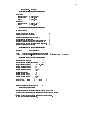
FILES le1 le2 le3 le4
INPUT variable type variable type ... variable type
TIME variable <variable <variable>>
CENSCODE variable value
discrete scale
idrec variable
truncate variable
timecov variable type values
convdt variable=variable{variable variable=variable{variable ...
class variables
joincode variable variable
timedep variable typedi
variable typedi
...
combine variable=variable+variable variable=variable+variable+variable ...
OUTPUT variables
future le5 le6
pedigree le7 le8 variable <variable>
formout type
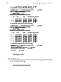
8.1 FILES Statement
FILES le1 le2 le3 le4
The FILES statement is used to dene the names of the les needed in the process of
data preparation for the actual survival analysis.
le1 is the name of the original data le (must exist in your directory).
le2 is the name of the recoded le produced by the program to be used by subse-
quent programs COX or WEIBULL. This le may be much larger than the original
data le when time dependent covariates are used in the analysis, as so-called elementary record are written spanning the times between any changes in time dependent covariates.
le3 is the name of a le containing the original and new codes (after internal
recoding) for each variable in the class statement. The le name is required even
when no class statement is dened. In this case it will be an empty le.
le4 is the name of a le containing information about the variables in the data
set to be used by subsequent COX or WEIBULL. (It is one of two parameter les
required by those programs).
13
Note for UNIX users: If the UPPER CASE ag in le parinclu (see later for a detailed
description of the parameters in parinclu) is set to .TRUE., all lowercase letters in the
parameter le are transformed into upper case internally (to avoid troubles with variable
names typed in dierent ways by the user). This implies that on systems where le
names are case sensitive (mainly UNIX), the le name of le1 has to be upper case to be
recognised by the program. Also, the names of the les produced by PREPARE (le2 to
le4) will be upper case even if stated lower case in the FILES statement.
If the UPPER CASE ag is set to .FALSE., all names (other than keywords, which can
be either upper or lower case) used in parameter les are case sensitive (they are not
transformed).
8.2 INPUT Statement
INPUT variable type variable type ... variable type
In the INPUT statement, variables names and their respective types are dened. The
input le (le1) is read in free format implying that variables have to be separated by
blanks and that all variables in the data set (whether needed or not in the current analysis)
have to be specied. Variable names may be up to 8 characters long (otherwise the name
is truncated), and may be comprised of any combination of characters, numbers and
symbols, except for the following symbols: +; = (). The following variable types are
allowed:
I4 - integer number
R4 - real number
D6 - date with 6 digits (ddmmyy)
D8 - date with 8 digits (ddmmyyyy)
Note that the "Y-2000 bug" is avoided for D6 dates by adding 100 to the value of "yy"
when yy is less than NBUG 2000 (set in the parinclu le).
8.3 TIME Statement
TIME variable < variable < variable >>
In the TIME statement, the dependent variable is dened. This is usually time, but may
be other things like lifetime production, etc. Time values of 0 should be avoided. The
time statement may have three dierent forms:
TIME variable
The variable must have been specied in the input statement and contains the time
14
CHAPTER 1. DATA PREPARATION PROGRAM (PREPARE)
till death or censoring of an individual (must be of type I4).
TIME variable1 variable2
variable1 is the time variable as above, variable2 is a date (D6 or D8) indicating
the beginning of the observation (must also be contained in list of input variables).
This is necessary for models with time dependent covariates when changes in risk
are given by dates and not by times in the TIMECOV or TIMEDEP statements.
TIME variable1 variable2 variable3
variable1 is the name of the time variable. It may or may not be contained in the list
of variables in the INPUT statement. variable2 and variable3 are dates (D6 or D8)
indicating the beginning and end of the observation. They must have been dened
in the INPUT statement. If variable1 is not found in the input statement, its value
will be calculated as dierence between end and beginning of the observation.
Note: Only one dependent variable may be specied. If dierent dependent variables are
of interest, separate analyses have to be run all of them starting with the data preparation
step.
8.4 CENSCODE Statement
CENSCODE variable value
In the CENSCODE statement, the censoring variable is dened. This is an indicator
variable. The variable name must be identical to one of the names specied in the INPUT
statement and must contain the censoring code (must be of type I4). value denes a
number indicating (right) censored records. All other values of the variable indicate
death (failure).
8.5 DISCRETE SCALE Statement
DISCRETE SCALE
The DISCRETE SCALE statement species that the failure time variable (variable1 in
the TIME statement) is expressed in discrete units with few (say, < 20) distinct values.
This is in preparation for, later on, an analysis using a grouped data model (Prentice and
Gloeckler, 1978) with the WEIBULL program (although it is not a Weibull model).
The immediate consequence of the DISCRETE SCALE statement is the implicit denition
and calculation of a time-dependent covariate called time unit, taking distinct values at
15
time 0 1 2 3 failure time ; 1. An elementary record is created for each value of this
time unit variable.
8.6 IDREC Statement
The statement can have two mutually exclusive alternative forms:
IDREC variable
IDREC STORE PREVIOUS TIME
In the IDREC statement, normally a variable is dened that is unique to each record.
This variable may be needed for sorting the elementary records when using a Weibull
model and is therefore obligatory when using WEIBULL as analysis program. The
variable must be of type I4.
Note: The same variable may also appear in the class statement (e.g., animal
identication for an animal model. In this case, the variable will appear twice in
the recoded le2 that is a result of this program (rst, unrecoded as the 3rd variable
on the record, and second, recoded as one of the class variables).
The alternate formulation (IDREC STORE PREVIOUS TIME) is needed in the
special case when later on in the WEIBULL program, a (log-gamma) random
time-dependent covariate is integrated out (and only then). The beginning of each
interval is then stored at the place where the identity of the record is normally
stored.
Note: if the "INTEGRATE OUT variable1 WITHIN variable2" statement is used
in the WEIBULL parameter le, the basic form "IDREC variable" is maintained
(no need of "STORE PREVIOUS TIME").
8.7 TRUNCATE Statement
In the TRUNCATE statement, information is provided for handling left truncated
records. For these records, the origin point (e.g. date of birth) is known but occurs
before the beginning of the study period, so that the covariate status between origin
point and begin of study period is unknown. It has the following form
TRUNCATE variable
variable holds the time of the truncation point. It must be of type I4, D6 or D8. If of
type I4, it species the time between the beginning of the observation and the point in
time when the individual actually entered the study (truncation point). If of type D6 or
D8, it holds the truncation date and time will be calculated as dierence between this
16
CHAPTER 1. DATA PREPARATION PROGRAM (PREPARE)
date and the date specied in the rst argument of the time statement (types must be
identical). If the variable is coded 0 in the data set, the record is treated as untruncated
(independently from data type).
Left truncated records are now (in version 3.0 and above) handled by both the WEIBULL
and the COX programs.
8.8 TIMECOV Statement
TIMECOV variable type values
The TIMECOV statement is needed when the hazard changes with time (this may be
calendar time or time as measured from the beginning of each observation) independent
from special (stochastic) events.
variable denes the name of the timecov variable. This must be a new name not
specied previously (in the INPUT or TIME statements).
type may be either integer (I4) or a date (D6 or D8).
values indicates a list of values (with a maximum number specied through the
parameter MAXFIG in the parinclu le) dening points in time when the hazard
changes.
If type is integer, values indicate changes in the hazard rate relative to the beginning
of each observation. If type is a date, it determines points in the calendar time, when
the risk changes for all individuals. The change on the time axis of the individual is
then calculated as dierence between the respective date given and the date indicating
the starting point of the observation in the TIME statement. Therefore, when using
a TIMECOV statement with type as a date, the TIME statement must hold the date
of the beginning of the observation as second argument and the date of the end of the
observation as third argument. The variable types of those arguments must be identical.
Note: Only one TIMECOV statement can be handled by the program (in version 3.0 and
above).
8.9 CONVDT Statement
CONVDT variable=variable{variable variable=variable{variable ...
With the CONVDT statement, the dierence between two date variables is calculated
and written onto a new time variable. The variable to the left of the equality sign must
be a new name, the variables to both sides of the minus sign must be dates of the same
17
type (D6 or D8). This statement will be used for calculation of covariates (e.g., age at
rst calving from date of birth and date of calving) but not for the dependent variable,
which is processed in the TIME statement.
Note: the variable to the left of the minus sign is the date later in time (e.g., date of rst
calving), to the right is the one earlier in time (e.g. date of birth).
8.10 CLASS Statement
CLASS variables
The CLASS statement lists the names the classication variables to be used in the analysis. Independent variables dened in the MODEL statements of the COX or WEIBULL
programs which are not dened in the CLASS statement will be treated as continuous
covariates. All variables dened in the class statement will be internally recoded (list of
codes in le3). Codes are transformed back to original values for the listing of the results
from COX and Weibull. The recoded values are needed, though, in the CONSTRAINTS
statement of COX and WEIBULL (see there).
8.11 JOINCODE Statement
JOINCODE variable variable
The JOINCODE statement species that the two variables indicated must be recoded
together, as if they pertained to a single list. This is necessary, e.g., when sires and
maternal grand-sires are specied as dierent variables in the input statement but must
appear in a single recoded list: sires can also appear as maternal grand-sires and their
additive genetic eect as grand-sires is 0.5 times their eect as sires. This is also one
way (out of 2) for the denition of sire-dam models: sires and dams are recoded together
using the JOINCODE option and an 'overall' relationship matrix is used for both sires
and dams.
Both variable names must have been declared previously in the CLASS statement.
8.12 TIMEDEP Statement
TIMEDEP variable typedi
variable typedi
.....
Time dependent covariates, i.e., independent variables whose value may change during
the time an individual is observed (may be CLASS or continuous covariates) are dened
with this statement. variable names must be dened in the INPUT statement.
18
CHAPTER 1. DATA PREPARATION PROGRAM (PREPARE)
In the input le (le1), any changes of value of these variables with time have to be given
at the end of each record as triplets in the following way (see also section about les):
consecutive number of the time dependent covariate. This means that one has to
count on which position in the record the variable (with its initial value) is located
and this value has to be supplied.
date or time of change in covariate value.
new covariate value.
typedi
relates to the way the dierence between beginning of the observation and the
actual change of the covariate is given. If it is I4, it is given as time, if it is D6 or D8, it
is calculated as the dierence between the date given in b) and the date describing the
beginning of the observation in the TIME statement (both dates must be of the same
type).
One of the most frequent problems (errors) that users encounter with the Survival Kitx"
is related to an inadequate preparation of these triplets (for example, with time of change
= 0 (or even 0) or dates of change before the origin (or the truncation) point or after
the failure date.
8.13 COMBINE Statement
COMBINE variable = variable + variable variable = variable + variable + variable:::
The COMBINE statement is used to to produce 'interaction eects' between two or three
variables dened in the CLASS statement. Continuous variables are not allowed. The
variable to the left of the equality sign must be a new name. If one of the variables
combined is time dependent (dened in the TIMEDEP statement), the resulting variable
will also be time dependent.
8.14 OUTPUT Statement
OUTPUT variables
In the OUTPUT statement, the variables dened in the variables list will be written to
the output le (le2 of the FILES statement). This le will then be used for the analysis
with the COX or WEIBULL programs. The variables must be of type I4 or R4 when
dened in the INPUT statement. All variables newly dened in subsequent statements
(TIME, CONVDT, COMBINE) are also allowed. No date variables (D6 or D8) may be
included into the output le!
19
8.15 FUTURE Statement
FUTURE le5 le6
In the FUTURE statement, you provide information about a set of records, for which you
want a printout on predicted values of the survivor curve (quantile values or functional
values of the survival function at given times).
le5 is the name of the original le holding the 'future' records (must exist in your
directory). The structure of the le must be exactly identical to that of le1
le6 is the name of the recoded le produced by the program identical in structure
to the le2 data le. It will be used by COX or WEIBULL to produce values related
to the corresponding survival functions. Note: if you have a future statement, you
also need to have an IDREC statement, as elementary records have to be sorted by
identity of the original records.
8.16 PEDIGREE Statement
In the PEDIGREE statement, you give information about a pedigree le for including
relationships between individuals into the model. Depending on the model to be used
later, it can have two alternative forms:
PEDIGREE le7 le8 variable
(for sire or animal models,
or for sire-dam models if "JOINCODE sire dam" is used)
PEDIGREE le7 le8 variable1 variable2
(for sire-dam models)
le7 is the name of the original pedigree le (must exist).
le8 is the name of the recoded pedigree le produced by the program.
variable is the name of the random variable (animal or sire) in the data le (must
be stated in INPUT and OUTPUT).
variable1 and variable2 (for sire-dam models, unless JOINCODE is used) are the
names of the sire and dam variables in the data le (must be stated in INPUT and
OUTPUT)
FORM OF THE PEDIGREE FILE:
The pedigree le has ALWAYS to consist of four columns:
CHAPTER 1. DATA PREPARATION PROGRAM (PREPARE)
20
1 { identity of animal
2 { sex code in sire-dam models (1 = male, 2 = female, -1 for group of unknown
parents ) may be used for other purposes in other situations
3 { identity of sire
4 { identity of dam (or maternal grandsire)
Unknown parents are dened as 0 or with negative values corresponding to groups of
unknown parents.
Important: there should be one line dened for each animal, each parent and each group
of unknown parents.
8.17 FORMOUT Statement
FORMOUT type
FORMOUT FIXED FORMAT In Fn.d
With the FORMOUT statement, the format of the recoded output les is specied (these
are le2 of the FILES statement and le6 of the FUTURE statement). If a xed format
is chosen, the type FIXED FORMAT must be followed by the Fortran description of
formats for integers and reals ("In Fn.d", e.g., "I8 F12.5" for integers with 8 digits and
reals with 12 digits, including 5 decimal gures). The other admitted types are:
FREE FORMAT
UNFORMATTED
BLOCKED UNFORMATTED
COMPRESSED
FREE FORMAT is the default option.
FIXED FORMAT is useful when you need to sort output les but your sorting
routine is not really adequate when the records are not strictly presented in columns
(especially on PCs). Be careful: if the formats for integers and/or reals are not big
enough, the results will be incorrect. Note: the previous way (version 2.0) to
produce a recoded le in xed format through a parameter in the parinclu le is no
longer available.
UNFORMATTED writes binary les. This saves time and (some) space when writing.
21
BLOCKED UNFORMATTED reads and writes NRECBLOC binary records to-
gether. NRECBLOC is specied in the parinclu le. It is the most ecient option:
it is much faster than when records are written or read one at a time.
With COMPRESSED, blocs are compressed before being written and decompressed
after being read).
COMPRESSED is available only when the program PREPAREC (calling subroutines for compression / decompression) is used. It takes about 3 times longer to
read and write compressed les but these are substantially smaller.
The BLOCKED UNFORMATTED and COMPRESSED options should not be used if
the output le(s) must be sorted. In this same situation, the UNFORMATTED option
can be used only if a binary sort subroutine is available.
9 Sorting of the recoded le
For the use in COX or (sometimes) in WEIBULL, the recoded le produced by PREPARE
(le2 of the FILES statement) has to be sorted. The sorting order is dierent for COX and
WEIBULL. A sorting routine is not included in the Survival Kit, as it is often machine
dependent. The specication of a xed format (FORMOUT FIXED FORMAT) may be
necessary when compiling the Survival Kit with some (PC) compilers, where the output
of a single record in free format is put into separate lines when it exceeds 80 characters.
You have to nd out!
9.1 COX Program
This is the sorting order (from highest to lowest level) for COX:
STRATA variable: in ascending order (this is necessary only when a STRATA
statement is used in COX see below)
TIME variable: in descending order (the TIME variable is always the rst variable
in the recoded le)
CENSCODE variable: in ascending order (the censoring variable is always the second variable in the recoded le)
This sort prevents the use of UNFORMATTED (on most computers), BLOCKED UNFORMATTED or COMPRESSED formats.
CHAPTER 1. DATA PREPARATION PROGRAM (PREPARE)
22
9.2 WEIBULL Program
Several special cases exist1 . These cases are mutually exclusive:
A STRATA statement is used in WEIBULL. The sorting order should be:
{ STRATA variable: in ascending order
{ IDREC variable: in ascending order (the IDREC variable is always the third
variable in the recoded le)
{ TIME variable: in ascending order (the TIME variable is always the rst in
the recoded le).
A LOGGAMMA random variable is dened in the WEIBULL parameter le. This
random variable is algebraically integrated out in order to reduce the number of
parameters to estimate or to obtain an exact marginal posterior distribution. This
is done using the INTEGRATE OUT statement in the parameter le (see below).
Again two situations exist:
{ If the INTEGRATE OUT statement is followed by the name of one variable
only (e.g., INTEGRATE OUT sire), the sorting order should be:
the variable to be integrated out: in ascending order
IDREC variable: in ascending order (the IDREC variable is always the
third variable in the recoded le)
TIME variable: in ascending order (the TIME variable is always the rst
in the recoded le).
Note that if the variable to be integrated out is time-dependent (e.g., herd-yearseason, the statement IDREC STORE PREVIOUS TIME must have been
used.
{ If the INTEGRATE OUT statement is followed by the name of two variables
(e.g., INTEGRATE OUT year WITHIN herd) and if the original records were
already sorted by herd, the statement IDREC STORE PREVIOUS TIME is
not needed, and there is no need to sort according to the variable "year".
Records should simply be sorted by IDREC variable and ascending TIME
variable. This is the natural way records are recoded and therefore, the need to
sort the elementary records disappears. This may lead to a substantial saving of
time and allows the use of UNFORMATTED, BLOCKED UNFORMATTED
or COMPRESSED formats.
1
also applies to the grouped data model of Prentice and Gloeckler (1978)
23
General case:
In all other situations, there is no need to sort: the recoded data set is naturally
recoded by IDREC variable and ascending TIME variable. This allows the use of
UNFORMATTED, BLOCKED UNFORMATTED or COMPRESSED formats.
9.3 Sorting of "future records"
The sorting of "future records" (le6 of the FUTURE statement) is identical to the sorting
order for WEIBULL (general case), irrespective of whether COX or WEIBULL is used
later on.
24
CHAPTER 1. DATA PREPARATION PROGRAM (PREPARE)
Chapter 2
Programs COX and WEIBULL
Depending on the parameterisation of the baseline hazard function, either program COX
or program WEIBULL may be called after data preparation with PREPARE. Using the
same recoded data set, various alternative survival analyses may be carried out with both
programs. The programs require two dierent parameter les. The rst is produced by
PREPARE. The second parameter le essentially describes the model of analysis. Most
statements used in the second parameter le may be called by both programs, a few
(mainly relating to estimation of the distributional parameters of log-gamma distributed
random eects) may only be called by WEIBULL. Generalized residuals are computed
only by COX.
As already mentioned, for extremely large applications for which the number of elementary records is huge a modied version of WEIBULL (weibullc.f, denoted hereafter
WEIBULLC) was written using public domain C subroutines for compressing and decompressing data during I/O operations (a similar version for the Cox model was not
implemeted as the Cox model is not suited for huge applications). Except for the format
specication in parameter le "1" (which is the direct result of the use of PREPAREC,
see above), the parameter les for WEIBULLC are exactly the same as for WEIBULL
10 Parameter le "1"
As pointed out above, this parameter le is produced by PREPARE (le4 of the FILES
statement of PREPARE). Note that you normally will not want to change anything in
this le. This section is written to aid the user in understanding the le.
10.1 Syntax
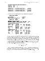
The following statements are used in this parameter le.
25
26
CHAPTER 2. PROGRAMS COX AND WEIBULL
TIME position
CODE position
ID position or PREVIOUS TIME position
COVARIATE variable nlevels pos1 pos2 variable nlevels pos1 pos2 ....
discrete scale
joincode variable1 variable2
format type
10.2 TIME Statement
TIME position
position is a gure which labels the position of the dependent (TIME) variable on the
recoded data le (le2 of the FILES statement of PREPARE).
Note: The position of the time variable is always 1.
10.3 CODE Statement
CODE position
position is a gure which labels the position of the censoring code on the recoded data
le (le2 of the FILES statement of PREPARE). In this le, censored records are always
coded 0, uncensored records are coded 1, but other codes are also used: ;2 for the
rst elementary record refering to a truncated observation, ;1 for an elementary record
indicating a change in a time-dependent covariate
Note: The position of the censoring code is always 2.
10.4 ID Statement and PREVIOUS TIME Statement
The two statements are mutually exclusive.
ID position
PREVIOUS TIME position
position labels the position of the record identication code (ID Statement) or of the
beginning of the time period for an elementary record in the special case described in the
IDREC STORE PREVIOUS TIME statement of program PREPARE (required when a
time-dependent covariate is integrated out in the WEIBULL program, and only then).
Note: The position of the identication variable is always 3.
27
10.5 COVARIATE Statement
COVARIATE variable nlevels pos1 pos2 variable nlevels pos1 pos2 ....
The COVARIATE statement gives information about the covariates that might be used in
the model of analysis. These are all variables in the OUTPUT statement of the PREPARE
parameter le except for the TIME and CODE variables described above.
The covariates are listed one per line, rst continuous and then class covariates. variable
is the name of the covariable, nlevels gives the number of dierent levels found for class
variables (zero for continuous covariates), and pos1 and pos2 give the position(s) of the
covariate on the recoded le (le2 in the FILES statement of the PREPARE parameter
le). When pos1 and pos2 are identical, the covariate is time independent. When pos1
and pos2 are dierent (subsequent) numbers, the covariate is time dependent and the
covariate values on pos1 and pos2 give the status of the covariate before and after the
chDange of the hazard function of an individual due to a change in this (or another) time
dependent covariate.
10.6 DISCRETE SCALE Statement
DISCRETE SCALE
The DISCRETE SCALE statement indicates that the recoded le is prepared to be used
with the WEIBULL program to t the grouped data model of Prentice and Gloeckler
(1978).
It is the direct result of the usage of the DISCRETE SCALE in the PREPARE parametesr
le. The consequence has been the denition of a specic time-dependent covariate called
time unit, which changes values at each time point (1 2 ) between the origin and the
observed failure time or censoring time. A corresponding number of elementary records
were therefore created.
The statement also avoids the need to repeat it in the user-supplied parameter le "2".
If one wants to run a regular Weibull model, one can simply comment out this statement
in parameter le "1". However, if a lot of elementary records were created because of
the denition of the time unit time dependent variable, it may be more ecient to start
again, running PREPARE after deleting the DISCRETE SCALE statement in its own
input parameter le.
10.7 JOINCODE Statement
JOINCODE variable1 variable2
28
CHAPTER 2. PROGRAMS COX AND WEIBULL
The JOINCODE statement indicates that the two variables variable1 and variable2 were
recoded together, in a single list. This is the case, e.g., when sires and maternal grand-sires
are specied as dierent variables but used in a sire-maternal grand sire model: sires may
appear as maternal grand-sires and their additive genetic eect as grand-sires is 0.5 times
their eect as sires. This statement is the direct result of the usage of the JOINCODE
statement in the PREPARE parameter le.
10.8 Format Statement
format type
format type displays the format of the recoded (output) les from PREPARE (in the PREPARE parameter les, these are le2 of the FILES statement and le6 of the FUTURE
statement).
If a xed format is chosen, format type is FIXED FORMAT and is followed by the Fortran
description of formats for integers and reals ("In Fn.d", e.g., "FIXED FORMAT I8 F12.5"
for integers with 8 digits and reals with 12 digits, including 5 decimal gures). The other
possible expressions for format type are:
FREE FORMAT
(= default)
UNFORMATTED
BLOCKED UNFORMATTED
COMPRESSED (only with PREPAREC/WEIBULLC)
11 Parameter le "2"
In this parameter le, the statistical model used in the data analysis is described together
with various options regarding storage, statistical tests and output. Most statements
and options are valid for both COX and WEIBULL programs. Therefore, the same
param eter le can be used with both programs. However, a few statements apply to only
one of these programs and should be commented out when the other program is run, in
order to avoid warning or error messages. These will be indicated below.
The grouped data model of Prentice and Gloeckler (1978) can also be tted using
the WEIBULL program, although it is not a Weibull model. For the user, the parameter le "2" has exactly the same form as for the Weibull model, the use of the
grouped data model being already specied in the parameter le "1" through the DISCRETE SCALE keyword. The latter will automatically generate an extra time-dependent
covariate time unit which will appear in the model (do not repeat it in the MODEL statement). Note that a few statements are not applicable to such a model (e.g., RHO FIXED
or INTEGRATE OUT),
29
11.1 Syntax
The following statements are used in this parameter le. Statements written in capitals are
obligatory. Names between < > are omitted when they are not needed. The sequence
of statements should be as shown.
Comments may be included in the parameter le. The start of a comment is /*, the end
is */, i.e. /* This text is a comment */. The text between the two delimiters may be on
more than one line.
Sometimes the statement or option names are longer than 8 characters (e.g., the statement
read old solutions shown below) In this case, only the rst 8 characters (i.e. read old
in our example) are signicant to the programs, the rest may or may not be written by
the user.
FILES le1 le2 le3 <le4 le5 le6>
title Title of analysis
strata variable
rho xed value
MODEL<variables>
coecient variablevalue <only >statistics
random variable <estimate <moments>> distribution <rules> parameter<s>
<repeat sequence for next variable<s>> integrate out < joint mode > variable1 < within variable2 >
include only variable value value
test <type<s> of test>
std error
dense hessian
baseline
kaplan
survival le7 le8 option
residual le7 le8
constraints options
convergence criterion
storage on disk or in core
store solutions
read old solutions
store binary
30
CHAPTER 2. PROGRAMS COX AND WEIBULL
11.2 FILES Statement
FILES le1 le2 le3 <le4 le5 le6>
The FILES statement is used to dene the names of the les needed for running COX or
WEIBULL.
le1 is the name of the recoded data le (le2 of FILES Statement in PREPARE). This
le must exist in your directory.
le2 is the name of the le containing the original and new codes (after internal recoding)
for each CLASS variable. (le3 of FILES Statement in PREPARE). The le name is
required even when no CLASS variables were dened in PREPARE. In this case it will
be an empty le.
le3 is the name of the output le where the results of the analysis are listed.
le4 is the (recoded) pedigree le le8 of the PEDIGREE Statement of PREPARE. This
le is not obligatory and will only be needed for analyses where the additive genetic
relationship structure between individuals is considered.
le5 is only needed when for very large applications, solutions from a previous run are to
be read in because the READ OLD SOLUTIONS statement is used (see below).
le6 is only needed when for very large applications, solutions are to be stored for a
subsequent run with the STORE SOLUTIONS statement (see below).
Files 1, 2 must exist in your directory, les 4 and 5 must exist when subsequent statements
make use of them le 3 and 6 will be new les (Note: existing les with the same name
are overwritten without warning). In situations where les 5 or 6 are required but not
les 4 or 4 and 5, dummy names have to be stated for the latter ones.
Note for UNIX users: Unless the UPPER CASE ag in le parinclu (see later for a
detailed descriptions of the parameters in parinclu) is set to .TRUE., all lowercase letters
in the parameter le are transformed into upper case internally (to avoid troubles with
variable names typed in dierent ways by the user). This implies that on systems where
le names are case sensitive (mainly UNIX), the le name of le1 has to be upper case
to be recognised by the program. Also, the names of the les produced by PREPARE
(le2 to le4) will be upper case even if stated lower case in the FILES statement. If
UPPER CASE is set to .FALSE. in le parinclu, le and variable names will not be
recognized if typed dierently.
11.3 TITLE Statement
TITLE Title of analysis
31
The TITLE of analysis may ll the rest of the line (up to position 80) after the statement
name. It will be written at the beginning of the output les (le3 of the FILES statement
above and le8 of the SURVIVAL statement below).
11.4 STRATA Statement
STRATA variable
Stratication is an extension of the proportional hazards model. With stratication, the
assumption of the proportionality of hazards is restricted to individuals within subgroups
of the population, where grouping is dened by the variable indicated in the STRATA
statement. Only one variable can be used as strata variable. If a combination of variables
is more sensible (e.g. year-season), the individual variables may be combined in the
COMBINE statement of PREPARE.
Note: Do not forget that in models with strata, data have to be sorted by strata (ascending) and within strata by the time variable (descending) and the censoring variable
(ascending). See section on Files, records and sorting.
11.5 RHO FIXED Statement
RHO FIXED value
This statement can be used only with the WEIBULL program (with COX, a warning
message is printed and the statement is ignored). It species a xed value for the Weibull
parameter . For example, RHO FIXED 1:0 will constrain to be 1, therefore
dening an exponential regression model instead of a more general Weibull model.
This statement is ignored when a grouped data model is tted (then is always assumed
to be 1).
11.6 MODEL Statement
MODEL < variables >
The MODEL statement species the independent variables aecting the dependent variable described in the TIME statement (remember that only one dependent variable may
be specied there). The variables listed must be a subset of the variables dened in the
COVARIATE statement of Parameter le 1.
Model building capabilities: Discrete (class) and continuous variables may be included.
32
CHAPTER 2. PROGRAMS COX AND WEIBULL
No covariate name at all is also accepted.
no covariate: if no variable is specied between MODEL and the semi-colon, the COX
model can be used to simply compute a nonparametric estimate of the survivor curve
(KAPLAN statement, see below) for each stratum. The WEIBULL program with no
covariate specied will lead to the t of a 2-parameter Weibull function for each stratum.
discrete covariates: they have to be stated in the CLASS and COMBINE statements of
the parameter le for PREPARE.
continuous covariates: all variables in the MODEL which have not been specied via
CLASS and COMBINE. Polynomial regression models may be tted by stating variable**N where N is the power to which the covariate value is taken. For example, for a
third order polynomial in varx, the statement would be:
MODEL varx varx**2 varx**3 + any number of other discrete and continuous covariates
Covariables are always automatically centered for computations (i.e. their mean value is
subtracted from each observation). For polynomial expressions, the values are rst taken
to the power of N, the mean value is then calculated and subtracted for this new variable.
The mean value (or the sum of mean values if there are more than just one continuous
covariate) is printed in the output of COX and is incorporated to the intercept in the
output of WEIBULL. This is important to know when you want to draw the regression
curves).
interactions between discrete covariates: They may only be tted by combining the original values of two or three variables into a new one via the COMBINE statement of
PREPARE.
Interactions between class and continuous covariates (i.e. individual regressions) and
nested models are currently not supported.
Variables are treated as xed unless they are stated in the RANDOM statement described
below.
When a grouped data model (= Prentice and Gloeckler's model) is tted, an extra timedependent covariate time unit will be automatically generated and will appear in the
model (do not repeat it in the MODEL statement). The purpose of this covariate is the
estimation of the baseline hazard function at the same time as the regression parameters.
11.7 COEFFICIENT Statement
COEFFICIENT <variable value <variable value> >
The COEFFICIENT statement species that the covariate variable will always be multiplied by the coecient value. This is especially useful when used in conjunction with
the statement JOINCODE in PREPARE. For example, a typical sire-maternal grand-sire
used in animal breeding will be obtained by specifying: JOINCODE sire mgs
(in the
33
data preparation parameter le, for PREPARE)
and
COEFFICIENT mgs 0.5
Also, the best possible way to dene a sire-dam model is:
JOINCODE sire dam
(in the data preparation parameter le, for PREPARE)
and
COEFFICIENT sire 0.5 dam 0.5 11.8 <ONLY >STATISTICS Statement
ONLY STATISTICS
STATISTICS
These statements can be used only with the WEIBULL program (they are ignored otherwise). They request the computation and the printing of a number of elementary statistics
related to each level of the class variables specied in the MODEL statement (number
of observations, number of observed failures, age at failure, average value of continuous
covariates for all observations and for the uncensored ones, etc..). If STATISTICS is
preceded by ONLY , the program will stop as soon as these values have been printed.
11.9 RANDOM Statement
RANDOM variable < ESTIMATE < MOMENTS >> distribution < rules >
parameter < s >< repeat previous sequence for next variable < s >>
The RANDOM statement gives information on variables to be treated as random. The
distribution parameters of the random covariates are either assumed to be known or they
may be estimated (optional parameter ESTIMATE).
distribution allows to specify the distribution that the random variable is assumed to follow. The user may choose from 3 alternatives:
LOGGAMMA: the levels of the random eect follow a log-gamma distribution. This is
identical with assuming a gamma frailty term. The frailty term, say w, is dened as a multiplicative term to the usual hazard function with xed eects only, i.e, w = expfz(t)ug.
NORMAL: the levels of the random eect are independently normally distributed. This
assumption is not so common in survival analysis but for rather large gamma parameters
( > 10), the log-gamma and normal are similar and the normal distribution is needed to
make the step to the multivariate normal distribution described next.
MULTINORMAL rules: the levels of the random eect follow a multivariate normal
distribution with covariances between levels being induced by genetic relationships.
34
CHAPTER 2. PROGRAMS COX AND WEIBULL
Two types of relationships are allowed and may be stated via the rules parameter:
USUAL RULES are the relationships under an animal model MGS RULES relate to
a sire model or a sire-maternal grandsire model, accounting for male relationships, . Note
that SIRE DAM MODEL that was used in earlier versions to relate sires and dams in a
sire-dam model in which sires and dams had been recoded separately is now obsolete and
not accepted any more. Instead, simply use the JOINCODE option in PREPARE.F and
...MULTINORMAL USUAL RULES sire ... for sire-dam models). When MULTINORMAL is used, information about the covariances between individuals has to be provided
via a pedigree le (le4 of the FILES statement).
parameter is the distribution parameter (gamma parameter with the log-gamma distribution and the variance with normal or multivariate normal distributions). It may be
preset, in which case one value of the parameter has to be provided or it may be estimated
(see ESTIMATE option below), in which case three values have to be given (see below)
ESTIMATE: when stated after the variable name, the distribution parameter is estimated as the mode of its marginal posterior density which is approximated by Laplacian
integration.
the parameter value is replaced by three values: the rst two values are the bounds of
the interval to be searched, the third value gives the nal tolerance (accuracy). Using the
ESTIMATE option, the parameter of only one random variable may be estimated at one
time. If the estimated value is at one of the bounds prespecied, a warning message is
printed and the analysis should be repeated changing the values of the bounds. (Example:
you stated parameters 0.01 0.1 0.001 as lower bound, upper bound and tolerance, which
means that the program must look for the mode of the marginal posterior density in
the interval ]0.01, 0.1 and the searching process is stopped when the current interval for
the estimate is smaller than 0.001. If the program output tells you "the mode is between
0.0100 and 0.0109 and the best value is 0.0104", you need to reset the bounds, e.g., to 0.005
and 0.011 and start again). The STORE SOLUTIONS and READ OLD SOLUTIONS
statements described below may be used to avoid starting from scratch again.
When the INTEGRATE OUT JOINT MODE statement is used (only with a Weibull
model and for a log-gamma random eect), the ESTIMATE statement should not be
used: the gamma parameter is then estimated jointly with the other eects after exact
algebraic integration of the log-gamma random eect.
MOMENTS: this option may be used together with ESTIMATE to compute estimated
mean, standard deviation and skewness of the marginal persterior value of the distributional parameter. The computation is based on an iterated Gauss-Hermite quadrature of
the approximate marginal posterior densities. The number of points used for the integration is NPGAUSS, which is specied in the parinclu le.
When the amount of information available for the estimation is limited, unpredictable
results (if any) may be obtained, although the mode of the distribution may have been
35
successfully computed.
11.10 INTEGRATE OUT Statement
INTEGRATE OUT < JOINT MODE > variable < WITHIN variable2 >
This option is only available in the WEIBULL program (the COX program prints an
error message and stops) and is not applicable to a grouped data model. When a random
eect is assumed to follow a log-gamma distribution in a Weibull model, it is possible to
algebraically integrate it out from the joint posterior density. This technique decreases
the number of parameters to estimate (sometimes drastically). Algebraic integration is
equivalent here to absorption of a group of equations in systems of linear equations. The
consequences are similar: a smaller system (but usually much less sparse) and no direct
availability of the estimates of the eects integrated out (other than the gamma parameter)
The INTEGRATE OUT statement can be used alone, i.e., only followed by the name
of the random variable to integrate out (must appear in the RANDOM statement too).
Then, the gamma parameter of the log-gamma distribution is assumed to be known. For
example,
MODEL e
ect1 e
ect2 e
ect3
RANDOM LOGGAMMA e
ect1 10.0
INTEGRATE OUT e
ect1
will lead to the integration of the log-gamma distributed random variable e
ect1 and the
estimation of eects e
ect2 and e
ect3 and of the Weibull parameters, assuming a value
of 10.0 for the gamma parameter of e
ect1.
If the INTEGRATE OUT statement is used with the JOINT MODE option, (as INTEGRATE OUT JOINT MODE e
ect1 in the example above) then the gamma parameter
is estimated jointly with the other eects as the mode of the marginal posterior distribution of the gamma parameter, e
ect2, e
ect3 and the Weibull parameters. The value 10.0
specied in the RANDOM statement is just used as a starting value in the optimisation
subroutine.
The advantage of this approach is that it performs exactly the marginalisation of the
random eect, which otherwise is done only approximately via Laplacian integration
(Ducrocq and Casella, 1996). Note, however, that the xed and other random eects
as well as the Weibull parameters still have to be integrated out if one wants the full
marginal posterior density for the gamma parameter of the log-gamma distribution).
The combined use of RANDOM ESTIMATE : : : and INTEGRATE OUT JOINT MODE
: : : oers an easy solution to the joint estimation of the distribution parameters of two
random variables.
36
CHAPTER 2. PROGRAMS COX AND WEIBULL
Note: In order to perform the algebraic integration, the recoded data le le 1 must be
sorted by increasing levels of the random eect to integrate out.
For very large datasets, this sorting according to the levels of the random eect to integrate
out may be cumbersome, in particular because it is not compatible with the use of the
BLOCKED UNFORMATTED and COMPRESSED options. An alternative approach
which avoids this sorting using the 'WITHIN' statement has been developed when the
eect to integrate out has a hierachical structure. This will be better illustrated through
the example of a random herd-year(-season) interaction eect.
The 'hard-work' approach is to have the herd and year eects included in the original data
le. The data preparation data le (for PREPARE) includes the following statements:
INPUT : : : herd I4 year I4 : : : :::
IDREC STORE PREVIOUS TIME
CLASS : : : herd year : : : COMBINE : : : hy = herd + year : : : OUTPUT : : : hy : : : FORMOUT FREE FORMAT
Each possible herd-year combination is recoded separately and the recoded data le has
to be sorted by increasing hy levels. The use of IDREC STORE PREVIOUS TIME is
necessary because the eect hy to integrate out is a time-dependent covariate (see the description of the IDREC STORE PREVIOUS TIME statement and the sorting rules). The
need to sort also forces the use of a free format for the output le. Then, in WEIBULL,
the integration of a random herd-year season eect implies the following statements (assuming a log-gamma distribution with initial parameter 10.0):
MODEL : : : hy : : : RANDOM hy LOGGAMMA 10.0 : : : INTEGRATE OUT JOINT MODE hy
The alternative (much easier) way simply requires that the initial data set be sorted by
herd (and by herd only). There is no need to recode each herd-year interaction separately,
no need to specify STORE PREVIOUS TIME, no need to restrict the output format to
free format, no need to sort the recoded le. The data preparation parameter le looks
like (for example):
INPUT : : : herd I4 year I4 : : : :::
IDREC animal id
37
CLASS : : : herd year : : : OUTPUT : : : herd year : : : FORMOUT BLOCKED UNFORMATTED
:::
and the parameter le "2" for WEIBULL:
MODEL : : : year : : : RANDOM year LOGGAMMA 10.0 : : : INTEGRATE OUT JOINT MODE year WITHIN herd
The output of these two approaches would be exactly the same.
11.11 INCLUDE ONLY Statement
INCLUDE ONLY variable value value
This option was developed in version 2.0 of the Survival Kit, almost exclusively for the
estimation of the gamma parameter of a log-gamma time-dependent random variable.
This was needed because the Weibull model dids not accept left truncated records. Now
that left truncated records are handled by WEIBULL as well, INCLUDE ONLY can be
regarded as obsolete.
11.12 TEST Statement
TEST <type<s> of test>
Hypothesis testing is generally performed via likelihood ratio tests. The following types
of tests may be requested by the TEST statement:
(GENERAL: test of the full model vs the model with no covariate. This is the default
option and will be used even without request.)
SEQUENTIAL : test of the eects included in the model in sequential order (i.e. depending on the sequence in the MODEL statement).
LAST: likelihood ratio test comparing the full model with models excluding one eect
at a time. This is done for each eect separately.
EFFECT list of variables: the same type of test as with LAST is performed, but only for
eects stated in the list.
SEQUENTIAL and LAST may be stated together. EFFECT may be stated either alone,
with SEQUENTIAL or with LAST. When EFFECT is used with LAST, it is redundant.
38
CHAPTER 2. PROGRAMS COX AND WEIBULL
If it is used with SEQUENTIAL, the sequential inclusion of the eects in the model one at
a time will start with the rst eect appearing in the MODEL statement which is stated
in the list following EFFECT. For example,
MODEL var1 var2 var3 var4 var5 var6
TEST SEQUENTIAL EFFECT var4 var5 var6
will lead to likelihood ratio tests corresponding to the sequential introduction of variables
var4, var5, var6.
11.13 STD ERROR and DENSE HESSIAN Statements
Asymptotic standard errors of estimates may be requested by the following statement:
STD ERROR
Be cautious with the use of the STD ERROR statement with large models as the Hessian matrix has to be calculated and stored to calculate standard deviations of estimates. In the case of the COX program or the WEIBULL program with the particular
DENSE HESSIAN statement, the full (square) Hessian matrix is stored. Its dimension
is specied by the parameter NDIMAX2 which is dened in the parinclu le and may
become limiting with respect to storage capacity. In the case of the WEIBULL program,
the Hessian matrix is stored in sparse form (unless the DENSE HESSIAN statement is
specied) and the vector space required in order to do so is specied by the parameters
AVAIL and NZE in the parinclu le. DENSE HESSIAN
The full storage of the square Hessian matrix is the only option when the COX program
is used (the DENSE HESSIAN statement is not required). The default option for the
WEIBULL program is the sparse storage of the Hessian, unless the DENSE HESSIAN
statement is used. In cases where the memory is not limiting or when a log-gamma
random eect is algebraically integrated out (leading to smaller but denser Hessian), the
DENSE HESSIAN option may save substantial computing time.
11.14 BASELINE Statement
BASELINE
The statement species that the baseline hazard, the baseline cumulative hazard and the
baseline survivor functions should be computed and printed, in the COX program. These
values are computed at each distinct value of the TIME variable. In stratied analyses
(use of the STRATA statement), separate baseline functions are calculated for strata.
39
With the WEIBULL program, the computation of the baseline Weibull parameters is
always implicit: the BASELINE statement is ignored.
11.15 KAPLAN Statement
KAPLAN
The statement species that the product-limit (=Kaplan-Meier) estimate of the survivor function should be computed and printed. The Kaplan-Meier estimator is a nonparametric population estimator of the survivor function that does not take into account
any of the eects stated in the MODEL statement. The KAPLAN statement is permitted
only with the COX program (it is ignored otherwise).
11.16 SURVIVAL Statement
SURVIVAL le7 le8 option<s>
The SURVIVAL statement may be used to get information about the survivor function
of individuals with specic covariate values. It is very useful to relate the estimated
regression coecients to a more conventional scale like median survival time or probability
of survival to a certain age.
le7 is the name of the recoded le produced by program PREPARE on request in the
FUTURE statement of PREPARE (called le6 there).
le8 holds the results invoked by the use of the SURVIVAL statement.
The following options may be used:
QUANTILES value<s>
With this option, times at which specic values (quantiles) of the survivor curve are
reached are calculated and printed for each individual specied in le7. The values must
lie between 0 and 100 and will be divided by 100 to produce the value of the survivor
function (e.g., with a value of 25, S(t)= 0.25). The median survival time can therefore be
requested by the option QUANTILE 50.
ALL TIMES
The estimate of the survivor curve will be computed at all times (= failure time or change
in time-dependent covariates) indicated for each individual in le7
EQUAL SPACE interval limit
The estimate of the survivor curve will be computed at equally spaced times for each
individual. two gures are needed: time interval and time limit. For example, SURVIVAL
EQUAL SPACE 5 100 will compute the value of the survivor curve at time 5, 10, 15, : : :
40
CHAPTER 2. PROGRAMS COX AND WEIBULL
95, 100.
SPECIFIC time<s>
The estimate of the survivor curve will be computed at the specied times indicated for
each individual.
Note: The statements SURVIVAL and RESIDUALS are mutually exclusive and should
not appear in the same parameter le.
11.17 RESIDUALS Statement
RESIDUALS le7 le8 The use of the RESIDUALS statement is (so far) limited to the COX program. It species
that the generalized residuals (Cox and Snell, 1966) of the records in le 7 should be
computed and printed in the output le le 8. If all generalized residuals are requested
(general case), le 7 is the unsorted recoded data le (direct output of PREPARE).
If the option STORAGE ON DISK is used, the output will also include the martingale
residuals and the deviance residuals (Klein and Moeschberger, 1997).
Note: The statements RESIDUALS and SURVIVAL are mutually exclusive and should
not appear in the same parameter le.
11.18 CONSTRAINTS Statement
CONSTRAINTS option
For models not of full rank (all models with xed discrete class covariates), constraints can
be imposed upon the eects to be estimated to get a set of meaningfull, easy to interpret
estimable eects. The program oers dierent options for setting those constraints:
LARGEST: the program will set to zero the level of each discrete covariate with the largest
number of uncensored failures. This is the default procedure of handling constraints.
FIND: the constraints are found by the program. This will guarantee the correct number
of constraints to produce a full rank Hessian matrix, so that the tests for the full model
as well as for individual eects are based on the correct degrees of freedom (however,
the constraints found do not guarantee an easy interpretation of the results...) Linear
dependencies in the Hessian matrix are found by performing a Cholesky decomposition.
For very large problems, the storage of this matrix may be a limiting factor (as for the
computation of the standard error see the STD ERROR statement).
NONE: no constraints specied (but implicit ones will appear if standard errors are to be
computed, i.e. a generalized inverse of the Hessian matrix will be used if needed).
41
IMPOSE <CHECK> variable rec level variable rec level ...: the constraints are supplied
by the user. variable denes the eect for which a constraint is to be set (must be a CLASS
variable that has been stated in the MODEL statement). rec level is the recoded value
of the eect that should be constraint.
Note: You have to look into the le that holds original and recoded levels of the CLASS
eects (le3 dened in the PREPARE parameter le) to look up what is the recoded value
of the level you actually want to put the constraint on. To do so, look for the name of
the eect of interest. Columns 4 (when there is no interaction), 4 and 5 (when two eects
were combined into an interaction) or 4, 5, and 6 (when three eects were combined)
display the original code. The last column denes the new code. By use of the option
check the program will check whether the constraints specied by the user make sense.
11.19 CONVERGENCE CRITERION Statement
CONVERGENCE CRITERION real number
The real number in the CONVERGENCE CRITERION statement provides the termination point for the optimisation routine used in the likelihood maximisation. Its default
value is parameter EPS BFDEF set in parinclu (usually, 1.D-8). Alternative values may
be invoked either by using this statement or by changing the value of EPS BFDEF in
parinclu.
Warning: an unnecessary strict convergence criterion set by the user will lead to a warning
message by the optimisation routine telling (amongst others) "LINE SEARCH FAILED",
although the results are printed and usually valid.
11.20 STORAGE Statement
STORAGE option
The data le le3 may either be read in and held in core (option IN CORE or while being
read for the rst time, be written out on a temporary le in binary mode on disk (option
ON DISK) for faster access in subsequent readings of the le in cases where the core
memory available is not big enough to hold the whole data le. The largest number of
elementary records possibly stored in core at the same time is specied by the parameter
NRECMAX in the parinclu le.
11.21 STORE SOLUTIONS and READ OLD SOLUTIONS Statement
STORE SOLUTIONS
42
CHAPTER 2. PROGRAMS COX AND WEIBULL
READ OLD SOLUTIONS
These two statements are only useful for very large applications (applications running
for hours and days). If the STORE SOLUTIONS statement has been used to write the
nal solutions to le6 of the FILES statement, the READ OLD SOLUTIONS statement
may be used in the next run to retrieve those solutions from le5 of the FILES statement.
The model does not need to be the same in both runs. This is mainly useful when one
is tting a complex model from a simpler one or in connection with the ESTIMATE
option of the RANDOM statement. When the results of the estimation indicate that
the true value of the distributional parameter for the log-gamma or Normal distributions
lies outside the prespecied interval, the values of the interval may be changed and using
READ OLD SOLUTIONS the optimisation may proceed from the point reached already.
For storage of solutions not only at the end of the optimisation procedure but after
each iteration, an alternative approach has to be taken. In the parinclu le, a character
parameter BACKUP is dened. This parameter may be used to dene the name of a
le where solutions will be stored each iteration. If the solutions are needed (e.g. in
a restart after a system shut-down), you only have to give the BACKUP lename as
le5 (they have exactly the same structure) in the FILES statement and include the
READ OLD SOLUTIONS statement in your parameter le.
11.22 STORE BINARY Statement
STORE BINARY
This statement is only useful for very large applications (applications running for hours
and days). The reading of binary les is much faster than the reading of les in free
format. If you have very large datasets which you may use for dierent types of repeated
analyses, it may therefore be useful to create and repeatedly read a binary version of the
recoded data le. This is easily done by specifying 'FORMOUT UNFORMATTED' or
'FORMOUT BLOCKED UNFORMATTED' in the data preparation parameter le (for
PREPARE), when the initial data le is recoded.
However, this strategy is often (in the case of FORMOUT UNFORMATTED) or always (in the case of FORMOUT BLOCKED UNFORMATTED) incompatible with the
sorting of the recoded le, for example when stratication or integration of a random
eect is envisioned. The statement STORE BINARY is a way to avoid this diculty:
with STORE BINARY in your parameter le, the program only reads le1 in free format and writes it (under the same name + .bin) as a binary (blocked unformatted)
le. Then the program will stop. In the new le, records are blocked together by
43
groups of size NRECBLOC, a parameter that is set (and may be changed) in parinclu. Then, you must change the format statement in parameter le "1" from what it is to
BLOCKED UNFORMATTED. In the subsequent runs, the STORE BINARY statement
is deleted and le1 is replaced by its new name (i.e., with .bin at the end). Note however that you cannot sort the blocked-binary le anymore. This means that the models
should not dier in the denition of the STRATA statement or of the INTEGRATE OUT
statement (these are sorting criteria).
Note: the statement READ BINARY used in previous versions of the Survival Kit is
now obsolete: the fact that the le to be read is unformatted is indicated in the parameter
le "1" used in COX or WEIBULL
44
CHAPTER 2. PROGRAMS COX AND WEIBULL
Chapter 3
The parinclu le
In the parinclu le,/indexparinclu parameters are dened which are used for dimensioning
of vectors and arrays. They may be redened to t your personal needs and computational
facilities. Criteria like iteration numbers and stopping rules are dened and may be
redened. Finally, le and directory names may be supplied for redirecting special input
and output les. The variables and their settings are explained subsequently. If you make
any changes to parinclu, you have to recompile prepare.f, cox.f and weibull.f (or preparec.f
and weibullc.f.
c***********************************************************************
c
Definition of parameters to used in the various programs of the
*
c
SURVIVAL KIT
*
c***********************************************************************
IMPLICIT NONE
c
c----------------------------------------------------------------------c----------------------------------------------------------------------c PARAMETERS THAT MAY BE MODIFIED BY THE USER
c Remember: when you change any of the parameters, you have to recompile
c your programs.
c----------------------------------------------------------------------c----------------------------------------------------------------------c
c
c Parameters related to the size of your problem
c ==============================================
c
INTEGER MXSTRA,NTIMMAX,NSTIMAX
45
46
CHAPTER 3. THE PARINCLU FILE
INTEGER NRECMAX,NRECMAX2,MXEF,MXEF_USED,NDIMAX,NDIMAX2
c
c-- NRECMAX = maximum number of elementary records
c-(Caution: with time-dependent variables this number may be much larger
c-than the number of records in your original data file!!)
c
PARAMETER(NRECMAX=100000)
c
c-- NRECMAX2 = maximum number of elementary records in the 'future'
c-data file (FUTURE statement in PREPARE).
c-These will normally be much fewer than in the data file
c
PARAMETER(NRECMAX2=100)
c
c-- MXEF = max. number of covariates. These are discrete
c-(CLASS) covariates and continuous covariates.
c-Time dependent covariates have to be counted twice (because
c-the states before and after change occupy two positions on
c-the recoded data file) !!
c
PARAMETER(MXEF=20)
c
c-- MXEF_USED = max. number of covariates actually used in the
c-MODEL statement of COX or WEIBULL.
c-There may be situations where you create recoded files with
c-very many covariates with PREPARE and never use all of them
c-together in COX or WEIBULL. In this case it may make sense
c-to have MXEF_USED smaller that mxef (it must not be larger!)
c-to save core memory space.
c
PARAMETER(MXEF_USED=10)
c
c-- MXSTRA= max. number of strata, i.e. levels of the strata variable
c-defined in the STRATA statement.
c
PARAMETER(MXSTRA=25)
c
c-- NDIMAX = max. total number of levels of effects in the model
c-(size of the vector of solutions)
c
PARAMETER(NDIMAX=200)
47
c
c-- NDIMAX2 = this parameter is used to indicate whether the Hessian
c-matrix is to be stored or not. It is used in COX and (WEIBULL with the
c-DENSE_HESSIAN statement).
c-The Hessian is needed to calculate standard deviations of estimated
c-effects (STD_ERROR statement) and to find dependencies (option FIND
c-in the CONSTRAINT statement).
c-In WEIBULL, the Hessian is normally stored in sparse form (see
c-parameters AVAIL and NZE below) except when stating DENSE_HESSIAN
c-ndimax2 = ndimax -> Hessian is needed (and fully stored)
c-ndimax2 = 1
-> Hessian is not needed (or sparsely stored)
c
c-vvvvvvvvvvvvvvvvvvvvvvvvvvvvvvvvvvvvvvvvvvvvvvvvvvvvvvvvvvvvvvvvvvvvvv
c-| CAUTION: this is likely to be a limiting parameter for the size |
c-| of your problem. An incorrect specification of this parameter is |
c-| is also one of the most frequent sources of errors when using the |
c-| Survival Kit !!
|
c-vvvvvvvvvvvvvvvvvvvvvvvvvvvvvvvvvvvvvvvvvvvvvvvvvvvvvvvvvvvvvvvvvvvvvv
c
c
PARAMETER(NDIMAX2=1)
PARAMETER(NDIMAX2=NDIMAX)
c
c-- NTIMMAX = largest possible value of the (dependent) time variable
c-this value is necessary as an upper limit for an efficient
c-comutation of log(time) and exp(time) and when calculating
c-functional values of the survivor curve (SURVIVAL statement
c-of COX and WEIBULL)
c
PARAMETER(NTIMMAX=6000)
c
c-- NSTIMAX = maximum number of distinct times or quantiles that
c-can be defined in the SURVIVAL statement options SPECIFIC
c-and QUANTILE.
c
PARAMETER(NSTIMAX=100)
c
c-- INTE_ST gives the possibility to integrate out one loggamma
c-random effect with the option INTEGRATE_OUT ... WITHIN ...
c-WHILE a STRATA statement is specified
c-INTE_ST=4 ==> usual case
c-INTE_ST=5 ==> STRATA + INTEGRATE_OUT .. WITHIN ...
c
PARAMETER(INTE_ST=4)
48
CHAPTER 3. THE PARINCLU FILE
c
INTEGER BLKSIZE,BLKSIZE0,BLKSIZE2
PARAMETER(BLKSIZE0=(MXEF+3)*NRECMAX)
PARAMETER(BLKSIZE=(MXEF_USED+INTE_ST)*NRECMAX)
PARAMETER(BLKSIZE2=(MXEF+4)*NRECMAX2)
c
c Parameters used in the lbfgs maximisationn routine
c ==================================================
c
INTEGER ITER_BF,MVEC_BF,NO_LOG
REAL*8 EPS_BFDEF
c-- MVEC_BF = number of vectors used to store the approximation of the Hessian
c-(rank of approx. Hessian = MVEC_BF). Values between 3 and 20 might be
c-used).
c
PARAMETER(MVEC_BF= 15)
c
c-- EPS_BSDEF = Default convergence criterion, may be overridden using
c-the CONVERGENCE_CRITERION statement in COX or WEIBULL.
c-(||GRADIENT||/FUNCTION < EPS_BS max(1,||BETA||)
c
PARAMETER(EPS_BFDEF=1.D-8)
c
c-- ITER_BF = maximum number of iterations.
c
PARAMETER(ITER_BF= 1000)
c
c-- NO_LOG relates to the parameter rho of the WEIBULL distribution.
c-no_log = 1 -> rho is used in the maximisation routine
c-no_log = 0 -> log(rho) is used in the maximisation routine
c
PARAMETER(NO_LOG=1)
c
c Parameters used in the numerical integration to get moments of the
c marginal posterior of a random effect variance parameter
c (when the MOMENTS option in the RANDOM statement is used)
c===================================================================
c
INTEGER NPGAUSS,NITER_GAUSS
c
c-- NPGAUSS = number of points used during Gauss-Hermite integration
c
(has to be between 3 and 5)
c
PARAMETER(NPGAUSS=5)
49
c
c-- NITER_GAUSS = number of iterations in the Gauss-Hermite integration
c
process
C
PARAMETER(NITER_GAUSS=5)
c
c
c Parameters relating to sparse storage of the Hessian matrix in WEIBULL
c ======================================================================
c
INTEGER NDIMSPAR
INTEGER AVAIL,NZE
c
c-- NDIMSPAR = working vector to store intermediate elements used in
c-the recoding in PREPARE or during the sparse computation of
c-the HESSIAN in Weibull
c-this should be a few times bigger than NDIMAX (no general rule)
c
PARAMETER(NDIMSPAR=NDIMAX*100)
c
c-- AVAIL = declared dimension of working vector IS (used in fspak.f,
c-the sparse matrix package of MISZTAL and PEREZ_ENCISO)
c-the required number is a function of the number of nonzero elements
c-of the HESSIAN matrix
c-(note: this is the dimension of a VECTOR, not a MATRIX)
c
PARAMETER(AVAIL=10000)
c
c-- NZE = declared dimension of the vector "HESSIAN" which includes
c-all nonzero elements of the matrix of second derivatives.
c-Often, one can take NZE = AVAIL
c-(note: this is the dimension of a VECTOR, not a MATRIX)
c
PARAMETER(NZE=10000)
c
c
c Parameters relating to the binary storage of the initial file when
c-the statement STORE_BINARY is used
c ======================================================================
INTEGER NRECBLOC
c
c-- nrecbloc = number of records per block when writting/reading
50
CHAPTER 3. THE PARINCLU FILE
c-- a binary file for fast I/O (statements STORE_BINARY and
c-- READ_BINARY)
c
PARAMETER(NRECBLOC=10000)
c
c Parameters related to the parameter file of PREPARE
c ===================================================
c
LOGICAL SUPPLY_INPUT0
CHARACTER*30 INPUT_FILE0
c
c-- Normally, the name of the parameter file will be requested by
c-- program PREPARE. The following parameters are designed to
c-- circumvent this request and start the program using a defined name
c-- for the parameter file
c
c-- SUPPLY_INPUT0 is a logical variable defining the way the name
c-of the parameter file is supplied= .true. if the name of the input
c-supply_file=.true. -> parameter file is supplied at running time
c-supply_file=.false. -> name of parameter file is defined in parinclu
c
PARAMETER (SUPPLY_INPUT0=.true.)
c
c-- INPUT_FILE0 = name of the parameter file (used only if
c-supply_file0 = .false.)
c
PARAMETER (INPUT_FILE0='PARM1')
c
c
c Parameters related to the parameter and report files in COX and WEIBULL
c =======================================================================
c
LOGICAL UPPER_CASE,DETAIL_IT
LOGICAL SUPPLY_INPUT1,SUPPLY_INPUT2,SUPPLY_OUTPUT
CHARACTER*30 INPUT_FILE1,INPUT_FILE2,OUTPUT_FILE
CHARACTER*100 TEMPDIR,BACKUP
c
c-- upper_case = .TRUE. if all words (including file names) used in the
c-parameter file are to be converted to upper case (otherwise, the
c-variables in the statements are case sensitive.
PARAMETER(UPPER_CASE=.false.)
c
51
c-- SUPPLY_FILE1 : logical variable = .true. if the name of parameter file 1
c-(provided by PREPARE) is supplied at running time (.false. if supplied
c-in parinclu)
c
PARAMETER (SUPPLY_INPUT1=.true.)
c
c-- INPUT_FILE1 : name of parameter file 1 (only if supply_file1=.false.)
c
PARAMETER (INPUT_FILE1='para')
c
c-- SUPPLY_FILE2 : logical variable = .true. if the name of parameter file 2
c-is supplied at running time (.false. if supplied in parinclu)
c
PARAMETER (SUPPLY_INPUT2=.true.)
c
c-- INPUT_FILE2 : name of parameter file 2 (used only if supply_file2=.false.)
c
PARAMETER (INPUT_FILE2='PARM2')
c
c-- SUPPLY_OUTPUT : logical variable = .true. if the name of the detailed output
c-(with information about iterations) is supplied at running time
c
PARAMETER (SUPPLY_OUTPUT=.true.)
c
c-- OUTPUT_FILE : name of output file (used only if supply_output=.false.)
c
PARAMETER (OUTPUT_FILE=' ')
c
c-- TEMPDIR : name of the directory used for temporary files
c-(= ' ' if = current directory)
c
PARAMETER (TEMPDIR=' ')
c
c-- BACKUP : name of the file used to backup solutions. Solutions
c-will be stored after each iteration and may be used to restart
c-the iteration procedure in case the machine breaks down during
c-the maximisation (you have to use the READ_OLD_SOLUTIONS statement
c-of COX or WEIBULL then). Only useful for very large applications.
c-backup = ' ' if no backup file should be produced.
c
PARAMETER (BACKUP='backup')
52
CHAPTER 3. THE PARINCLU FILE
c
c-- DETAIL_IT : switch on (if = .true.) or off (if =.false.) the
c-printing of detailed information (for each effect) at each iteration
c-of the maximization subroutine (average,mean or max absolute change
c-between iterations)
PARAMETER (DETAIL_IT=.false.)
c
c----------------------------------------------------------------------c----------------------------------------------------------------------c PARAMETERS THAT MAY _NOT_ BE MODIFIED BY THE USER
c Don't you dare look beyond this point !!! :-)
c----------------------------------------------------------------------c----------------------------------------------------------------------c
c Parameters related to the reading and translation of parameter files
c ====================================================================
c
INTEGER MAXWORD,MAXLENG,MAXFIG,LRECL,NBUG_2000
INTEGER NKEYFE,NKEYC,NKEYW
c
c-- maxword = max. number of words in the parameter file
c-- maxleng = max. number of characters in a word
c-- maxfig = max. number of figures (i.e. numbers) in the parameter file
c-- lrecl = number of columns read per record
c-- nbug_2000 = maximum year value (yy=00==>nbug_2000) under which a D6 date
c-is transformed from ddmmyy to ddmm(100+yy)
C-to avoid the 'year 2000 bug'
c-- parameter files should be automatically transformed to upper-case names
c-- nkeyfe = number of keywords (i.e. statement types) used in the
c-parameter file for PREPARE
c-- nkeyc = number of keywords used in the parameter file for COX
c-- nkeyc = number of keywords used in the parameter file for WEIBULL
PARAMETER(MAXWORD=1000)
PARAMETER(MAXLENG=40)
PARAMETER(MAXFIG=400)
PARAMETER(LRECL=80)
PARAMETER(NBUG_2000=40)
PARAMETER(NKEYFE=17)
PARAMETER(NKEYC=61)
PARAMETER(NKEYW=61)
Chapter 4
A small example
The following (completely articial) example will be used to illustrate how to analyze
survival data using the Survival Kit.
1. Inital data le small.dat:
Consider the data le:
1
2
3
4
5
6
7
8
9
10
11
5
10
11
11
15
15
17
19
21
21
28
1
1
1
0
1
1
1
1
1
0
1
1
1
1
1
2
2
1
1
2
2
2
0
0
0
0
0
0
0
0
0
0
0
1
1
1
0
0
1
0
0
0
1
1
5 4 10
5 6 10
5 6 10
5 6 10
5 15 10
5 15 10
As specied in the INPUT line of the data preparation parameter le (small.par,
see below), the rst variable for each line corresponds to the animal identication
number (not necessarily from 1 to n as it is the case here). The second represents failure or censoring time. The third is the censoring code (here, 0=censored).
Column 4 refers to the level of sex eect and column 5 to the level of treatment
eect. It is assumed that treatment does not start at time 0 but later on. Hence,
the treatment variable is considered as a time-dependent covariate. This explains
why the fth column is always 0 here: the animal is not treated at t=0. The next
column indicated the number of changes in time-dependent covariates. Here, there
is only 1 change per animal, at most. When there is a change (column 6 = 1), a
triplet follows indicating the column number of the relevant covariate (column 5 =
'treatment'), the time of change (e.g., t=4 for record 1) and the new value of the
covariate (10, here): at time 4, the treatment level for animal 1 changes from the
value 0 to the value 10.
53
CHAPTER 4. A SMALL EXAMPLE
54
2. Data preparation parameter le small.par
This is the le that will be used as input for the PREPARE program.
/* FILE NAMES */
FILES small.dat small2.dat small.nco
/* VARIABLE NAMES */
INPUT id I4 longev I4 code
small.paa I4 sex I4 treat I4
/* TIME VARIABLE */
TIME longev /* CENSORING CODE */
CENSCODE code 0
/* TIME DEPENDENT COVARIATES
TIMEDEP treat I4
*/
/* IDENTIFICATION VARIABLE FOR EACH RECORD */
IDREC id
/* DISCRETE VARIABLES */
CLASS treat sex
/* DEFINITION OF AN INTERACTION */
COMBINE s_by_t= sex + treat
/* LIST OF RECODED VARIABLES */
OUTPUT longev id code treat sex s_by_t
/* FORMAT OF THE OUTPUT FILE */
FORMOUT FREE_FORMAT
The treatment variable is explicitely dened as a time-dependent covariate, with
changes indicated as integers (I4), not dates. The COMBINE statement denes a
new variable s by t, representing the interaction of sex by treatment. The id does
not appear in the CLASS statement and therefore will not be recoded.
3. Log le from the PREPARE program
The le name small.par is typed when PREPARE asks for an input le. The log
le indicates that 17 elementary (recoded) records were created (> 11, because
treatment is time-dependent. The number of classes is also indicated for the discrete
(class) variables.
Records read from input data file
11
Elementary records written
17
Class variable treat
with
2 classes
Class variable sex
with
2 classes
Class variable s_by_t
with
4 classes
REMINDER: File small2.dat
Sorting order:
has to be sorted for the use of COX.
55
Strata variable, ascending (only if strata are used)
Time variable, descending
Censoring variable, ascending
4. Recoded data set small2.dat
4 -1 1 1 2 1 1 2
5 1 1 2 0 1 2 0
6 -1 2 1 2 1 1 2
10 1 2 2 0 1 2 0
6 -1 3 1 2 1 1 2
11 1 3 2 0 1 2 0
11 0 4 1 0 1 1 0
15 1 5 1 0 2 3 0
6 -1 6 1 2 2 3 4
15 1 6 2 0 2 4 0
17 1 7 1 0 1 1 0
19 1 8 1 0 1 1 0
21 1 9 1 0 2 3 0
15 -1 10 1 2 2 3 4
21 0 10 2 0 2 4 0
15 -1 11 1 2 2 3 4
28 1 11 2 0 2 4 0
The structure of this le is given in le small.paa which is an output le of the
PREPARE program and an input les for the programs COX and WEIBULL - see
below). The rst column is the time of failure, of censoring, of change in at least
one time-dependent covariate, or of truncature (for truncated records). These four
categories are indicated by a code in column 2 with value 1, 0, -1 or -2 respectively.
The third column indicates the id number. The remaining ones correspond to
the covariates used, individually recoded from 1 to the total number of levels, for
discrete covariates. When a covariate is time-dependent, two columns are used, one
corresponding to the value of the covariate before the change and the next one for
after the change. For example, for animal 1 (rst elementary record), at time 4, the
level of the treatment eect changes (code= -1) from recoded value 1 to recoded
value 2 (columns 4 and 5) while the level for the s by t eect changes also from 1 to
2 (columns 7 and 8). At time 5 (second elementary record), animal 1 fails (code=
1).
5. parameter le "1" (for COX and WEIBULL) small.paa
This le is created by the PREPARE program. It explains the structure of the
small2.dat recoded le.
TIME
1
CODE
2
ID
3
COVARIATE
/* class variables */
treat
2
4
5
sex
2
6
6
s_by_t
4
7
8
FREE_FORMAT
CHAPTER 4. A SMALL EXAMPLE
56
For example, there are 2 levels of treatment stored in columns 4 (before any change)
and 5 (after the change). The sex eect is time-independent: only one column (6)
is needed.
6. le small.nco
This le is also an output le from the PREPARE program. It gives the orrespondence between old and new codes.
treat
treat
sex
sex
s_by_t
s_by_t
s_by_t
s_by_t
2
2
2
2
4
4
4
4
1
1
1
1
2
2
2
2
0
10
1
2
1
1
2
2
0
0
0
0
0
10
0
10
0
0
0
0
0
0
0
0
11
6
6
5
6
3
5
3
1
2
1
2
1
2
3
4
For each level of a discrete covariate, the name of the covariate (e.g., s by t for the
last line) is followed by the total number of levels of this eect (4), the number
of columns involved in its description (2, because it is a 2-term interaction) and
the corresponding original codes (sex 2 x treatment 10). Up to 3 eects can be
combined into an interaction. Column 7 indicates the number of elementary records
found with this particular level of the covariate (3) and column 8 (last one) gives
the new code (4).
7. recoded data set for COX small2s.dat
This is the recoded data set small2.dat after sorting by decreasing time change
(column 1) and increasing codes (column 2) (no stratication assumed).
28 1 11 2 0 2 4 0
21 0 10 2 0 2 4 0
21 1 9 1 0 2 3 0
19 1 8 1 0 1 1 0
17 1 7 1 0 1 1 0
15 -1 10 1 2 2 3 4
15 -1 11 1 2 2 3 4
15 1 5 1 0 2 3 0
15 1 6 2 0 2 4 0
11 0 4 1 0 1 1 0
11 1 3 2 0 1 2 0
10 1 2 2 0 1 2 0
6 -1 2 1 2 1 1 2
6 -1 3 1 2 1 1 2
6 -1 6 1 2 2 3 4
5 1 1 2 0 1 2 0
4 -1 1 1 2 1 1 2
8. parameter le "2" for COX
57
/* FILES
*/
FILES small2s.dat small.nco small.rco
/* TITLE
*/
TITLE SMALL EXAMPLE - COX MODEL
/* MODEL
MODEL sex treat */
/* TEST
TEST SEQUENTIAL LAST /* STANDARD ERROR
STD_ERROR
*/
*/
/* OTHER COMPUTATIONS
*/
BASELINE
RESIDUAL small2.dat small.res
The input data le is the sorted, recoded data le small2s.dat. The model simply includes sex treatment eects (no interaction here). The results will be stored
in small.rco. Likelihood ratio tests will be performed, comparing models with no
covariates, with sex only and sex and treatment (TEST SEQUENTIAL) and comparing the full model with restricted model (excluding sex = with treatment only
and excluding treatment = with sex only TEST LAST). After computing the regression coecients using Cox's partial likelihood, the baseline will be computed
(BASELINE) and generalized residuals will be calculated for all records in the unsorted le small2.dat and they will be stored in the small.res le.
9. log le from COX
This le appears on the screen terminal if the answer 'NONE' or ' ' is given when
a name for the detailed output le is requested.
The le starts with the names of the 2 input parameter les and other le names,
followed by a brief list of characteristics of the data set, of the model and some
elementary statistics.
parameter file: small.paa
parameter file: small.cox
*****************************************
SMALL EXAMPLE - COX MODEL
*****************************************
FILES USED :
RECODED DATASET
NEW/OLD CODES
OUTPUT
:
:
:
small2s.dat
small.nco
small.rco
CHAPTER 4. A SMALL EXAMPLE
58
RESIDUALS :
RECODED DATASET
OUTPUT
:
:
small2.dat
small.res
*****************************************
NO STRATIFICATION
FAILURE TIME READ IN COLUMN :
CENSORING CODE READ IN COLUMN :
1
2
IDENTIFICATION NUMBER READ IN COLUMN :
TOTAL NUMBER OF COVARIATES =
CONTINUOUS COVARIATES INCLUDED IN THE ANALYSIS =
DISCRETE COVARIATES INCLUDED IN THE ANALYSIS =
COVARIATES READ BUT NOT INCLUDED IN THE ANALYSIS =
POWERS OF CONTINUOUS COVARIATES
=
3
3
0
2
1
0
************** COX MODEL ****************
COVARIATE
1 sex
2 treat
CHARACTERISTICS
: DISCRETE TIME-INDEPENDENT READ IN COLUMN
: DISCRETE TIME-DEPENDENT READ IN COLUMNS
CONVERGENCE CRITERION USED =
6
4 (BEFORE T) AND
5 (AFTER T)
.10000D-07 (= DEFAULT VALUE)
********** SIMPLE STATISTICS ************
TOTAL NUMBER OF STRATA =
TOTAL NUMBER OF ELEMENTARY RECORDS =
RIGHT CENSORED RECORDS
MINIMUM CENSORING TIME
MAXIMUM CENSORING TIME
AVERAGE CENSORING TIME
:
:
:
:
2 ( 18.182%)
11
21
16.000
UNCENSORED RECORDS :
MINIMUM FAILURE TIME :
MAXIMUM FAILURE TIME :
AVERAGE FAILURE TIME :
EFFECT : sex
EFFECT : treat
MIN =
MIN =
1
17
9
5
28
15.667
1
1
MAX =
MAX =
2
2
Then the rst few recoded elementary records are printed, as well as the constraints
used (here the COX program chose to set to zero level 1 of sex and level 10 of
treatment, because they are the levels with the largest number of uncensored observations).
DATA
1 |
2 |
3 |
4 |
5 |
6 |
7 |
:
28
21
21
19
17
15
15
1 0
0 0
1 0
1 0
1 0
-1 0
-1 0
|
|
|
|
|
|
|
2 0
2 0
1 0
1 0
1 0
1 2
1 2
59
8
9
|
|
15 1 0
15 1 0
|
|
1 0
2 0
NUMBER OF ELEMENTARY RECORDS KEPT =
17
******* CONSTRAINTS ******
THE SOLUTION FOR THE FOLLOWING (RECODED) LEVELS IS SET TO 0:
(= LEVEL WITH LARGEST NUMBER OF UNCENSORED FAILURES FOR EACH EFFECT)
(WARNING : THE VALIDITY OF THESE CONSTRAINTS IS NOT CHECKED.
IN CASE THEY ARE MORE DEPENDENCIES,
THE DEGREES OF FREEDOM IN THE TEST(S) BELOW ARE INCORRECT)
EFFECT sex
EFFECT treat
LEVEL
LEVEL
1
10
Then limited storage quasi-Newton (Liu and Nocedal, 1989) minimization of FUNCT=
minus the likelihood function starts for each (sub-)model. GNORM is the norm of
vector of rst derivative of FUNCT. CONV. CRITERION is equal to:
GNORM=max(1 FUNCT ):
Let CC be the requested convergence criterion. The program stops the minimization process in the following situations:
CONV. CRITERION is less than 0.01 * CC
CONV. CRITERION is less than CC and the total number of FUNCT evalu-
ations is at least equal to the number of corrections (15, below)
After many attemps (usually 20), the program fails to nd a smaller value of
FUNCT. This is very often due to too strict a convergence criterion. A careful
examination of the variation of the FUNCT value during the last iterations will
help to reveal that. If FUNCT is still varying substantially, the program failed
to nd a proper minimum (often because the model is incorrect or inconsistent).
If FUNCT is stable, one can safely assume that the results are correct and that
a minimum has been found.
DATA :
*************************************************
N=
4
NUMBER OF CORRECTIONS=15
INITIAL VALUES
F= 1.488D+01
GNORM= 2.289D+00
*************************************************
I
NFN
1
2
3
4
5
2
3
4
5
6
FUNCT
1.341197562D+01
1.327040139D+01
1.326918347D+01
1.326917728D+01
1.326917728D+01
GNORM
6.570D-01
5.823D-02
4.121D-03
3.349D-05
1.974D-08
STEPLENGTH CONV. CRITERION
4.369D-01
1.000D+00
1.000D+00
1.000D+00
1.000D+00
4.898D-02
3.128D-03
2.154D-04
1.747D-06
1.030D-09
CHAPTER 4. A SMALL EXAMPLE
60
6
7
1.326917728D+01
9.451D-14
1.000D+00
4.930D-15
THE MINIMIZATION TERMINATED WITHOUT DETECTING ERRORS.
CONVERGENCE AFTER
6 EVALUATIONS OF FUNCTION FCOX IN
*************************************************
N=
4
NUMBER OF CORRECTIONS=15
INITIAL VALUES
F= 1.488D+01
GNORM= 1.534D+00
*************************************************
I
NFN
1
2
3
4
2
3
4
5
FUNCT
GNORM
1.411382471D+01
1.411350211D+01
1.411350124D+01
1.411350124D+01
3.266D-02
1.696D-03
2.899D-07
2.847D-12
.00 SECONDS
STEPLENGTH CONV. CRITERION
6.517D-01
1.000D+00
1.000D+00
1.000D+00
2.314D-03
1.202D-04
2.054D-08
2.017D-13
THE MINIMIZATION TERMINATED WITHOUT DETECTING ERRORS.
CONVERGENCE AFTER
4 EVALUATIONS OF FUNCTION FCOX IN
*************************************************
N=
4
NUMBER OF CORRECTIONS=15
INITIAL VALUES
F= 1.411D+01
GNORM= 2.542D+00
*************************************************
I
NFN
1
2
3
4
5
6
7
8
2
3
4
5
6
7
8
9
FUNCT
GNORM
1.230257068D+01
1.172877696D+01
1.170091695D+01
1.169961281D+01
1.169943368D+01
1.169943364D+01
1.169943364D+01
1.169943364D+01
1.122D+00
2.155D-01
6.500D-02
2.672D-02
3.665D-04
9.265D-06
1.296D-07
2.662D-10
.00 SECONDS
STEPLENGTH CONV. CRITERION
3.934D-01
1.000D+00
1.000D+00
1.000D+00
1.000D+00
1.000D+00
1.000D+00
1.000D+00
6.511D-02
8.071D-03
2.212D-03
8.924D-04
1.226D-05
3.099D-07
4.334D-09
8.905D-12
THE MINIMIZATION TERMINATED WITHOUT DETECTING ERRORS.
CONVERGENCE AFTER
8 EVALUATIONS OF FUNCTION FCOX IN
VALUE OF F =
11.6994336385
TIME FOR THE COMPUTATION OF THE HESSIAN =
.00 SECONDS
TIME FOR NUMERICAL FACTORIZATION =
.00 SECONDS
TOTAL TIME =
.01 SECONDS
.05 SECONDS
******* BYE - BYE ********
10. Results from COX
The beginning is exactly the same as the log le (les names, model characteristics,
simple statistics, constraints).
*****************************************
61
SMALL EXAMPLE - COX MODEL
*****************************************
FILES USED :
RECODED DATASET
NEW/OLD CODES
OUTPUT
:
:
:
small2s.dat
small.nco
small.rco
RESIDUALS :
RECODED DATASET
OUTPUT
:
:
small2.dat
small.res
*****************************************
NO STRATIFICATION
FAILURE TIME READ IN COLUMN :
CENSORING CODE READ IN COLUMN :
1
2
IDENTIFICATION NUMBER READ IN COLUMN :
TOTAL NUMBER OF COVARIATES =
CONTINUOUS COVARIATES INCLUDED IN THE ANALYSIS =
DISCRETE COVARIATES INCLUDED IN THE ANALYSIS =
COVARIATES READ BUT NOT INCLUDED IN THE ANALYSIS =
POWERS OF CONTINUOUS COVARIATES
=
3
3
0
2
1
0
************** COX MODEL ****************
COVARIATE
1 sex
2 treat
CHARACTERISTICS
: DISCRETE TIME-INDEPENDENT READ IN COLUMN
: DISCRETE TIME-DEPENDENT READ IN COLUMNS
6
4 (BEFORE T) AND
********** SIMPLE STATISTICS ************
TOTAL NUMBER OF STRATA =
TOTAL NUMBER OF ELEMENTARY RECORDS =
RIGHT CENSORED RECORDS
MINIMUM CENSORING TIME
MAXIMUM CENSORING TIME
AVERAGE CENSORING TIME
:
:
:
:
2 ( 18.182%)
11
21
16.000
UNCENSORED RECORDS :
MINIMUM FAILURE TIME :
MAXIMUM FAILURE TIME :
AVERAGE FAILURE TIME :
EFFECT : sex
EFFECT : treat
MIN =
MIN =
1
17
9
5
28
15.667
1
1
NUMBER OF ELEMENTARY RECORDS KEPT =
MAX =
MAX =
2
2
17
******* CONSTRAINTS ******
THE SOLUTION FOR THE FOLLOWING (RECODED) LEVELS IS SET TO 0:
(= LEVEL WITH LARGEST NUMBER OF UNCENSORED FAILURES FOR EACH EFFECT)
(WARNING : THE VALIDITY OF THESE CONSTRAINTS IS NOT CHECKED.
IN CASE THEY ARE MORE DEPENDENCIES,
5 (AFTER T)
CHAPTER 4. A SMALL EXAMPLE
62
THE DEGREES OF FREEDOM IN THE TEST(S) BELOW ARE INCORRECT)
EFFECT sex
EFFECT treat
LEVEL
LEVEL
1
10
CONVERGENCE AFTER
6 EVALUATIONS OF FUNCTION FCOX IN
.00 SECONDS
CONVERGENCE AFTER
4 EVALUATIONS OF FUNCTION FCOX IN
.00 SECONDS
CONVERGENCE AFTER
8 EVALUATIONS OF FUNCTION FCOX IN
.01 SECONDS
The rst part of the results includes all the likelihood ratio tests :
*******
RESULTS
********
-2 LOG LIKELIHOOD
STANDARDIZED NORM OF GRAD(-2 LOG L) =
*******
TESTS
23.39886728
.00000
********
LIKELIHOOD RATIO TEST FOR H0: BETA = 0
MODEL CHI2 =
6.368872
WITH
2 DF
(PROB >CHI2 =
R2 OF MADDALA (=MEASURE OF EXPLAINED VARIATION) =
.4395
LIKELIHOOD RATIO TESTS : SEQUENTIAL
VARIABLE
TOTAL
-2 LOG LIK
Z
DF
INCLUDING Z
NO COVARIATE 0
sex
1
treat
2
29.76773961
26.53835455
23.39886728
LIKELIHOOD RATIO TESTS : LAST
VARIABLE
TOTAL
-2 LOG LIK
Z
DF
EXCLUDING Z
sex
treat
1
1
28.22700247
26.53835455
CHI2
DELTA
DF
3.2294
3.1395
1
1
CHI2
DELTA
DF
4.8281
3.1395
1
1
PROB
>CHI2
.0723
.0764
PROB
>CHI2
.0280
.0764
.0414)
R2 OF
MADDALA
.2544
.4395
R2 OF
MADDALA
.1307
.2544
For example, when the treatment eect is added to a model with sex as only covariate, the full model includes sex + treatment while the restricted model includes
sex only and the corresponding likelihood ratio statistic has a value of 3.1395. This
statistic follows a chi-square distribution with 1 degree of freedom under H0 (treatment eects=0) with a corresponding p-value of 0.07. The R2 OF MADDALA is a
measure of proportion of explained variation by the model (Maddala, 1983, quoted
by Schemper, 1992). Its formal denition is:
;
R2M = 1 ; LR=LU
2=n
where n denotes the total sample size and LR and LU represent the restricted and
unrestricted (full model) maximum likelihoods, respectively. Under moderate censoring, R2M can be grossly interpreted as the usual R2 for linear models.
63
Then the estimates of the regression coecients are presented, followed by their
asymptotic standard error, a chi-square statistic (=square of estimate/standard error) for a Wald test of each particular regression coecient i (which tests i = 0),
with its associated p-value. The risk ratio is the exponential of the estimate of the
regression coecient. The last column indicates the number of uncensored records
for each level (it is related to the standard error of the estimate).
******* SOLUTIONS ********
COVARIATE :
1
2
sex
1
2
(DISCRETE)
treat
0
10
(DISCRETE)
ESTIMATE STANDARD
ERROR
CHI2
PROB
>CHI2
RISK UNCENSORED
RATIO FAILURES
.0000
-2.0251
*
1.0316
*
3.85
*
.0496
1.000
.132
5
4
-1.5583
.0000
.9027
*
2.98
*
.0843
*
.210
1.000
4
5
For example, females (sex = 2) are at a 1:=:132 = 7:577 lower risk of dying than
males (sex = 1).
For ease of interpretation, it is a good idea to impose constraints to force the
computation of specic contrasts. For example, one may be interested in evaluating
the increase in risk of males compared to females and not treated compared to
treated, by choosing non treated females as a reference. This is done by using the
CONSTRAINTS IMPOSE : : : statement in the parameter le small.cox. To dene
the proper constraints, one has to look in the small.nco le: sex 2 (old code) is
recoded as 2 (new code) and treatment 0 (old code) is recoded as 1 (new code). If
we add:
CONSTRAINTS IMPOSE sex 2 treat 1
to small.cox and running COX, we now get:
******* SOLUTIONS ********
COVARIATE :
ESTIMATE STANDARD
ERROR
1
sex
1
2
(DISCRETE)
2
treat
0
10
(DISCRETE)
CHI2
PROB
>CHI2
RISK UNCENSORED
RATIO FAILURES
2.0251
.0000
1.0316
*
3.85
*
.0496
*
7.577
1.000
5
4
.0000
1.5583
*
.9027
*
2.98
*
.0843
1.000
4.751
4
5
CHAPTER 4. A SMALL EXAMPLE
64
Now, it directly appears that males are 7.577 times more likely to fail than females
and that treated animals are at a 4.751 times higher risk than non treated ones.
The contrasts between males and females or between treated and non treated animals remain the same. The baseline however is changed. The one reported below
corresponds to the situation without explicit constraints.
******* BASELINE
********
CUMULATIVE HAZARD FUNCTION AND SURVIVOR FUNCTION FOR STRATUM
TIME
CUMULATIVE
SURVIVOR
HAZARD
FUNCTION
5
10
11
15
17
19
21
28
TOTAL TIME =
.45633
.80420
1.33765
4.34920
5.75223
7.74329
11.17092
18.74770
1
.63361
.44745
.26246
.01292
.00318
.00043
.00001
.00000
.05 SECONDS
11. Residuals for the Cox model
The generalized residuals of Cox and Snell (1966) are calculated for all records of
the unsorted small2.dat le. If the model is correct, they are distributed according to
a censored exponential distribution with parameter 1. This can be checked globally
by plotting the cumulated hazard distribution (- log S(RES)) or the expected order
statistics of the unit exponential distribution against the value of RESIDUALS. This
should result in a straight line going through the origin and with slope 1. Note that
expected order statistics are computed only when STORAGE IN CORE is used.
ANIMALS
AT RISK
11
9
8
7
6
5
3
2
1
TOTAL
FAILED
1
2
3
4
5
6
7
8
9
FAILURE RESIDUALS
1
1
1
1
1
1
1
1
1
.1208301
.3103519
.4439302
.4563280
.5264675
.9773750
1.2108388
1.6299547
2.0211752
S(RES)
-LOG S(RES)
.9090909
.8080808
.7070707
.6060606
.5050505
.4040404
.2693603
.1346801
.0000000
.0953102
.2130932
.3466246
.5007753
.6830968
.9062404
1.3117055
2.0048527
INF
EXPECTED
ORDER STAT.
.0909091
.2020202
.3270202
.4698773
.6365440
.8365440
1.1698773
1.6698773
2.6698773
It is also possible to get individual residuals, i.e., for each observation, including
martingale and deviance residuals by simply specifying STORAGE ON DISK in
the small.cox le.
65
TIME
ANIMAL
5
10
11
11
15
15
17
19
21
21
28
1
2
3
4
5
6
7
8
9
10
11
CENSORING
CODE
1
1
1
0
1
1
1
1
1
0
1
STRATUM GENERALIZED
RESIDUAL
1
.4563280
1
.4439302
1
.9773750
1
.2815734
1
.1208301
1
.5264675
1
1.2108388
1
1.6299547
1
.3103519
1
1.0211752
1
2.0211752
MARTINGALE
RESIDUAL
.5436720
.5560698
.0226250
-.2815734
.8791699
.4735325
-.2108388
-.6299547
.6896481
-1.0211752
-1.0211752
DEVIANCE
RESIDUAL
.6940770
.7155672
.0227979
-.7504310
1.5711144
.5797123
-.1976130
-.5317941
.9802044
-1.4291083
-.7968640
12. parameter le "2" for Weibull
The following parameter le small.wei now replaces small.cox:
/* FILES
*/
FILES small2.dat small.nco small.rwe
/* TITLE
*/
TITLE SMALL EXAMPLE - WEIBULL
MODEL /* MODEL
MODEL sex treat */
STATISTICS
/* TEST
TEST SEQUENTIAL LAST /* STANDARD ERROR
STD_ERROR
*/
*/
13. results from WEIBULL
The beginning is similar to the Cox outputs, except that here, raw statistics by level
of each discrete factor included in the model are given:
*****************************************
SMALL EXAMPLE - WEIBULL
MODEL
*****************************************
FILES USED:
RECODED DATASET
NEW/OLD CODES
OUTPUT
:
:
:
small2.dat
small.nco
small.rwe
*****************************************
FAILURE TIME READ IN COLUMN :
CENSORING CODE READ IN COLUMN :
1
2
CHAPTER 4. A SMALL EXAMPLE
66
IDENTIFICATION NUMBER READ IN COLUMN :
TOTAL NUMBER OF COVARIATES =
CONTINUOUS COVARIATES INCLUDED IN THE ANALYSIS =
DISCRETE COVARIATES INCLUDED IN THE ANALYSIS =
COVARIATES READ BUT NOT INCLUDED IN THE ANALYSIS =
POWERS OF CONTINUOUS COVARIATES
=
3
3
0
2
1
0
**************** MODEL ******************
COVARIATE
1 sex
2 treat
CHARACTERISTICS
: DISCRETE TIME-INDEPENDENT READ IN COLUMN
: DISCRETE TIME-DEPENDENT READ IN COLUMNS
6
4 AND
5
********** SIMPLE STATISTICS ************
TOTAL NUMBER OF WEIBULL PARAMETERS TO COMPUTE =
TOTAL NUMBER OF RECORDS =
11
TOTAL NUMBER OF ELEMENTARY RECORDS =
17
RIGHT CENSORED RECORDS
MINIMUM CENSORING TIME
MAXIMUM CENSORING TIME
AVERAGE CENSORING TIME
:
:
:
:
2 ( 18.182%)
11
21
16.000
UNCENSORED RECORDS :
MINIMUM FAILURE TIME :
MAXIMUM FAILURE TIME :
AVERAGE FAILURE TIME :
EFFECT : sex
EFFECT : treat
MIN =
MIN =
1
9
5
28
15.667
1
1
MAX =
MAX =
2
2
===========
1 WEIBULL PARAMETER(S) RHO WILL BE ESTIMATED
CONVERGENCE CRITERION USED =
.10000D-07 (= DEFAULT VALUE)
NUMBER OF ELEMENTARY RECORDS KEPT =
17
********** STATISTICS /LEVEL ************
EFFECT
1
sex
1
2
2
treat
0
10
NUMBER
%
OF
INDIVIDUALS
6
5
OBSERVED
FAILURES
%
AGE AT
FAILURE
TOTAL
TIME
%
AVERAGE
TIME
54.55
45.45
5
4
55.56
44.44
12.40
19.75
73.
100.
42.20
57.80
12.17
20.00
11 100.00
6 54.55
4
5
44.44
55.56
18.00
13.80
135.
38.
78.03
21.97
12.27
6.33
Note that these statistics should be interpreted with caution for time-dependent
covariates: for example, here, 11 individuals had a record with level of treatment
67
eect = 0 (all animals at t=0) while 6 of them also had a record with level of
treatment eect = 10...
******* CONSTRAINTS ******
THE SOLUTION FOR THE FOLLOWING (RECODED) LEVELS IS SET TO 0:
(= LEVEL WITH LARGEST NUMBER OF UNCENSORED FAILURES FOR EACH EFFECT)
(WARNING : THE VALIDITY OF THESE CONSTRAINTS IS NOT CHECKED.
IF THEY ARE MORE DEPENDENCIES, DEGREES OF FREEDOM IN TEST(S) BELOW ARE INCORRECT)
EFFECT sex
EFFECT treat
LEVEL
LEVEL
1
10
CONVERGENCE AFTER
19 EVALUATIONS OF FUNCTION FWEIB IN
.02 SECONDS
CONVERGENCE AFTER
16 EVALUATIONS OF FUNCTION FWEIB IN
.03 SECONDS
CONVERGENCE AFTER
17 EVALUATIONS OF FUNCTION FWEIB IN
.02 SECONDS
*******
RESULTS
********
-2 LOG LIKELIHOOD
STANDARDIZED NORM OF GRAD(-2 LOG L) =
*******
TESTS
55.40054940
.00000
********
LIKELIHOOD RATIO TEST FOR H0: BETA = 0
MODEL CHI2 =
6.479457
WITH
4 DF
(PROB >CHI2 =
R2 OF MADDALA (=MEASURE OF EXPLAINED VARIATION) =
.4451
LIKELIHOOD RATIO TESTS : SEQUENTIAL
VARIABLE
TOTAL
-2 LOG LIK
Z
DF
INCLUDING Z
NO COVARIATE 2
sex
3
treat
4
61.88000661
57.93613232
55.40054940
LIKELIHOOD RATIO TESTS : LAST
VARIABLE
TOTAL
-2 LOG LIK
Z
DF
EXCLUDING Z
sex
treat
3
3
61.28410415
57.93613232
CHI2
3.9439
2.5356
CHI2
5.8836
2.5356
DELTA
DF
1
1
DELTA
DF
1
1
PROB
>CHI2
.0470
.1113
PROB
>CHI2
.0153
.1113
.1661)
R2 OF
MADDALA
.3013
.4451
R2 OF
MADDALA
.0527
.3013
The main dierence iin WEIBULL compared to COX is the inclusion of estimates
of the Weibull parameter and log (called INTERCEPT here). These two
parameters fully describe the baseline hazard function and the baseline survivor
function S0(t) = expf;(t) g.
******* SOLUTIONS ********
WEIBULL PARAMETER(S):
CHAPTER 4. A SMALL EXAMPLE
68
FOR STRATUM
1 ==>
INTERCEPT =
RHO =
-8.07086
COVARIATE :
1
sex
1
2
(DISCRETE)
2
treat
0
10
(DISCRETE)
TOTAL TIME =
3.38225
STE =
STE =
.97667
2.65373
ESTIMATE STANDARD
ERROR
CHI2
PROB
>CHI2
.0000
-2.1895
*
1.0001
*
4.79
*
.0286
1.000
.112
5
4
-1.2901
.0000
.8108
*
2.53
*
.1116
*
.275
1.000
4
5
.10 SECONDS
RISK UNCENSORED
RATIO FAILURES
Chapter 5
Analysis of very large data sets
This section includes some advice to eciently analyze very large data sets.
12 PREPARE program
Usually, computing time and memory requirements related to the PREPARE program
are not limiting factors. The only potential problem that may occur is related to the size
of the output (recoded) data le, because the use of time-dependent covariates may lead
to a much larger number of elementary records (corresponding to each time interval for
which all time-dependent covariates remain constant) than the actual number of records
in the initial data set. In order to limit the size of the recoded data set:
1. in the OUPUT statement, specify only the covariates that you will need later
2. because (at this stage) the PREPARE program requires all main eects to be included in the OUTPUT statement when an interaction is created with the COMBINE statement, it may be advantageous to recode the interactions beforehand, if
the main eects are not to be used later. In contrast, if the interaction eect is
going to be treated as a random, log-gamma eect that will be integrated out in a
Weibull model, it is possible to avoid the recoding of the interaction in PREPARE
if INTEGRATE OUT : : : WITHIN : : : is used later on.
3. for extremely large applications, the program PREPAREC with the statement FORMOUT COMPRESSED should be prefered as the output (recoded) le will be
written in compressed format, using C subroutines. In some applications, the
compressed le may be 20 to 30 times smaller but computing times are typically
increased by a factor 2.5 to 3.
69
70
CHAPTER 5. ANALYSIS OF VERY LARGE DATA SETS
Also, unless when an individual random eect is to be tted later on, the ID number
should not be recoded, i.e., it should not appear in the CLASS statement (only in the
IDREC and OUTPUT statements).
13 Before running the COX or WEIBULL programs
1. In order to limit memory requirements, it is essential to accurately specify some
parameters in the parinclu le. In particular:
NRECMAX (maximum number of elementary records stored in core at one
time). This number should be relatively large (in particular, it should be
larger or equal to the exact number of elementary records if the statement
STORAGE IN CORE is used). However, for obvious reasons, this number
should not exceed the memory capacity.
MXEF USED (maximum number of covariates actually used in the MODEL
statement of COX or WEIBULL). Often, the recoded les created with PREPARE contain many variables but these are never actually used together in
COX or WEIBULL. In such a case, MXEF USED should be equal to the strict
maximum number of eects tted together.
2. For fast Input / Output:
I/O operations on free formatted les are relatively slow. In order to e-
ciently read and write the data le, the options UNFORMATTED or (even
better) BLOCKED UNFORMATTED should have been used in PREPARE
or the STORE BINARY statement should be used the rst time COX or
WEIBULL is run. In the latter case, the recoded data le is copied as a
blocked binary le (and the format in the rst parameter le must be changed
to BLOCKED UNFORMATTED). NRECBLOC records are written and read
together. This parameter is specied in the parinclu le. It should be rather
large (several thousands) in order to play the role of a buer but not irrealistically large (e.g., if NRECBLOC=100000 when the actual number of records
is 100001 will lead to the writing and reading of two blocks of size 100000 !!)
When the STORAGE ON DISK statement is used, a blocked binary temporary
le is created with NRECMAX records by block. Again, NRECMAX should
be large but not too large. If space is limiting on the directory where the
programs are run, the name of a "work" directory should be specied in the
parinclu le (parameter TEMPDIR).
71
14 COX and WEIBULL programs
1. If the assumption of a Weibull baseline hazard function is reasonable, it is highly
recommended to use a Weibull model instead of a Cox model, in particular when
standard errors or distribution parameters of random eects are requested.
2. In order to decrease the size of the vectors of parameters:
Use stratication if possible (STRATA statement).
With WEIBULL, when a random eect is included in the model whose estimates are not really needed, a loggamma prior should be used if possible,
and the eect should be integrated out (INTEGRATE OUT statement): this
is analogous to the absorption of the equations corresponding to the specied
eect in a linear system of equations. Note that like for an "absorption", the resulting Hessian matrix is no longer very sparse. Hence, the DENSE HESSIAN
statement should also be used.
3. To limit the number of iterations or function evaluations required:
Store solutions at the end of each run (STORE SOLUTIONS statement) or
use backup les (BACKUP parameter in the parinclu le). Start the next run
from the old solutions (READ OLD SOLUTIONS statement).
If only a few eects are added to a "well known" model, don't use the time
consuming TEST SEQUENTIAL or TEST LAST statements which specify
that all the eects in the model should be tested, starting from scratch . Use
the TEST <SEQUENTIAL> EFFECTS : : : statement instead.
Check that the convergence criterion is not too strict, by looking at the evolution of -(Log-likelihood), the function which is mimized to get the parameters
estimates (CONVERGENCE statement). Be careful, however: an incorrect
concergence criterion may lead to incorrect results.
With WEIBULL, the use of the RHO FIXED statement should lead to a faster
convergence rate.
4. When estimating the hyperparameter(s) of the distribution(s) of random eects:
When a loggamma prior is used with the INTEGRATE OUT statement, the
JOINT MODE option (which computes the gamma parameter jointly with the
other eects) should be prefered (faster convergence).
Don't choose huge initial intervals or too strict nal tolerances with the ESTIMATE statement.
Use the MOMENTS statement only if necessary or at least after a run to nd
the mode of the marginal posterior distribution of the hyperparameter.
72
CHAPTER 5. ANALYSIS OF VERY LARGE DATA SETS
Bibliography
Cox, D. (1972). Regression models and life table. J. Royal Stat. Soc. , Series B, 34:187{
220. with discussion.
Cox, D. R. and Oakes, D. (1984). Analysis of survival data. Chapman and Hall, London,
UK.
Cox, D. and Snell, E. J. (1966). A general denition of residuals. J. Royal Stat. Soc. ,
Series B, 30:248{275. with discussion.
Ducrocq, V. and Casella G. (1996). A Bayesian nalysis of mixed survival models. Genet.
Sel. Evol., 28: 505-529.
Ducrocq, V. and Solkner, J. (1994). "The Survival Kit", a FORTRAN package for the
analysis of survival data. In: 5th World Cong. Genet. Appl. Livest. Prod., Volume 22,
pages 51{52. Dep. Anim. Poultry Sci., Univ. of Guelph, Guelph, Ontario, Canada.
Ducrocq, V. and Solkner, J. (1998). "The Survival Kit { V3.0", a package for large
analyses of survival data. In: 6th World Cong. Genet. Appl. Livest. Prod., Volume 27,
pages 447{448. Anim. Genetics and Breeding Unit, Univ. of New England, Armidale,
Australia.
Kalbeisch, J. D. and Prentice, R. L. (1980). The statistical analysis of failure time data.
John Wiley and sons, New-York, USA.
Klein, J. P. and Moeschberger, M. (1997). Survival analysis. Springer-Verlag, New-York,
USA.
Liu, D. C. and Nocedal, J. (1989). On the limited memory BFGS method for large scale
optimization. Mathematical Programming, 45:503{528.
Maddala, G. S. (1983). Limited-dependent and quantitative variables in econometrics
Cambridge Univ. Press, UK.
73
74
BIBLIOGRAPHY
Perez-Enciso, M., Mizstal, I., and Elzo, M. A. (1994). Fspak: an interface for public
domain sparse matrix subroutine. In: 5th World Cong. Genet. Appl. Livest. Prod.,
Volume 22, pages 87{88. Dep. Anim. Poultry Sci., Univ. of Guelph, Guelph, Ontario,
Canada.
Prentice, R. and Gloeckler, L. (1978). Regression analysis of grouped survival data with
application to breast cancer data. Biometrics, 34:57{67.
Schemper M. (1992). Further results on the explained variation in proportional hazards
regression. Biometrika, 79:202{204.
Index
convergence criterion, 73
CONVERGENCE CRITERION, 43, 50,
61
COVARIATE, 29
COX, 8, 13, 23, 27, 30, 59, 73
Cox model, 6
**, 34
/*, */, 13, 31
parinclu le, 9, 13, 40, 45, 72
algebraic integration, 36, 37
ALL TIMES, 41
animal id, 17
animal model, 21, 36
AVAIL, 40, 51
BACKUP, 44, 53, 73
BASELINE, 41, 59, 66
baseline, 6, 7
binary le, 23, 44
BLOCKED UNFORMATTED, 22, 24, 25,
30, 38, 44, 72
Bug year 2000, 10, 15, 54
C subroutines, 8, 27, 71
case sensitive, 15, 32
CENSCODE, 16
censored record, 16
CHECK, 43
CLASS, 19, 34, 56
class variable, 7, 29, 34
CODE, 28, 57
COEFFICIENT, 35
COMBINE, 20, 34, 38, 56
comment, 13, 31
compile, 9
COMPRESSED, 8, 22{25, 30, 38, 71
CONSTRAINT, 8, 42, 60, 65
continuous variable, 7, 19, 29, 34
CONVDT, 19
convergence, 43, 50, 61
data preparation, 56
date, 13, 15, 18{20
degrees of freedom, 42
DENSE HESSIAN, 40, 73
DETAIL IT, 53
deviance residual, 8, 42, 66
discrete scale, 6, 9, 10, 16, 29, 30
discrete variable, 7, 19, 29, 34
DISCRETE SCALE, 10, 16, 29, 30
EFFECT, 40, 73
elementary record, 13, 17, 56, 71
elementary records, 29
EPS BFDEF, 43, 50
EQUAL SPACE, 42
ESTIMATE, 35, 36, 38, 73
explained variation, 64
FILES, 14, 32
FIND, 42
FIXED FORMAT, 22, 30
format, 22, 30
FORMOUT, 22
frailty, 6, 7, 36
FREE FORMAT, 22, 30
fspak, 40, 51
FUTURE, 21, 25, 41
75
76
Gauss-Hermite quadrature, 37
GENERAL, 39
generalized residual, 8, 27, 42, 66
genetic parameter estimation, 36
goodness-of-t test, 66
group of unknown parents, 22
grouped data, 6, 9, 10, 16, 24, 29, 30, 33,
34, 37
hazard function, 6
herd-year eect, 38
ID, 28
IDREC, 17, 21, 25, 28, 38, 56, 72
IMPOSE, 43, 65
IN CORE, 43, 72
INCLUDE ONLY, 39
INPUT, 15, 55
INPUT FILE, 52, 53
INTE ST, 47
INTEGRATE OUT, 17, 24, 36{38, 71, 73
interaction, 20, 34, 38, 56, 71
intercept, 34
ITER BF, 50
JOINCODE, 19, 21, 30
JOINT MODE, 36, 38, 73
KAPLAN, 34, 41
Kaplan-Meier estimate, 41
Laplacian integration, 36
large dataset, 6, 8, 27, 38, 44, 71
LARGEST, 42
LAST, 40, 59
likelihood ratio test, 8, 39, 59, 64
LINE SEARCH FAILED, 43
log-gamma distribution, 7, 17, 24, 27, 35{
38, 40
LOGGAMMA, 24, 35
Maddala, 64
martingale residual, 8, 42, 66
INDEX
MAXFIG, 18
MGS RULES, 36
minimization, 8, 61
MODEL, 34, 59
MOMENTS, 36, 73
MULTINORMAL, 36
multivariate normal distribution, 7, 36
MVEC BF, 50
MXEF, 48
MXEF USED, 48, 72
MXSTRA, 48
NBUG 2000, 10, 15, 54
NDIMAX, 49
NDIMAX2, 40, 49
NDIMSPAR, 51
new code, 32, 58
NITER GAUSS, 50
NONE, 43
NORMAL, 36
normal distribution, 7, 36
NPGAUSS, 37, 50
NRECBLOC, 23, 45, 52, 72
NRECMAX, 43, 48, 72
NRECMAX2, 48
NSTIMAX, 49
NTIMMAX, 49
number of corrections, 50
NZE, 40, 51
ON DISK, 43, 72
ONLY STATISTICS, 35
OUTPUT, 20
OUTPUT FILE, 53
partial likelihood, 6
PC, 23
PEDIGREE, 21, 32
polynomial regression, 34
prediction, 21
Prentice and Gloeckler's model, 6, 9, 10,
16, 24, 29, 30, 33, 34, 37
INDEX
PREPARE, 8, 13, 56, 71
PREPAREC, 8, 9, 23, 30, 71
PREVIOUS TIME, 28
proportional hazards model, 6, 7, 33
QUANTILES, 41
Quasi-Newton, 8, 61
R2 of Maddala, 64
RANDOM, 35, 38
random eect, 7, 17, 24, 35{37, 40
random eects, 6{8, 17, 24
rank, 42
READ BINARY, 45
READ OLD SOLUTIONS, 32, 36, 44, 73
relationship matrix, 7, 19, 21, 36
RESIDUALS, 42, 59, 66
results, 32
RHO FIXED, 33, 73
risk ratio, 65
second() (timing subroutine), 9
SEQUENTIAL, 39, 59
sire model, 21, 36
sire-dam model, 19, 21, 35, 36
sire-mgs model, 19, 21, 30, 35, 36
SIRE DAM MODEL, 36
sort, 23, 33, 38, 44, 58
sparse matrix, 8, 40, 51, 61, 73
SPECIFIC, 42
standard error, 8, 40, 65
STATISTICS, 35, 67
STD, 40
STD ERROR, 40
STORAGE, 43, 72
STORE BINARY, 72
STORE PREVIOUS TIME, 17, 25, 28,
38
STORE SOLUTIONS, 32, 36, 44, 73
STRATA, 23, 24, 33, 41, 73
strata, 7
SUPPLY INPUT, 52, 53
77
SUPPLY OUTPUT, 53
SURVIVAL, 41
syntax, 27
TEMPDIR, 53, 72
TEST, 39, 59, 73
TIME, 15, 28, 57
time-dependent, 6, 7, 13, 17, 18, 20, 24,
29, 55, 69
time unit, 10, 17
TIMECOV, 16, 18
TIMEDEP, 16, 20
TITLE, 33
triplet, 20, 55
TRUNCATE, 17
truncated record, 17, 57
UNFORMATTED, 22, 24, 25, 30, 44, 72
UPPER CASE, 15, 32
USUAL RULES, 36
variable name, 15
variable type, 15
variance parameter, 36
Wald test, 65
WEIBULL, 8, 13, 24, 27, 30, 67, 73
Weibull distribution, 6, 7, 17
WEIBULLC, 8, 9, 27, 30
WITHIN, 17, 37{39, 71