Download A User's Guide to - Parent Directory

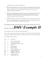
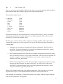
A User's Guide to
DMU
A Package for Analysing
Multivariate Mixed Models.
Version 6, release 5.2
Per Madsen & Just Jensen
Center for Quantitative Genetics and Genomics
Dept. of Molecular Biology and Genetics,
University of Aarhus
Research Centre Foulum
Box 50, 8830 Tjele
Denmark
Email: [email protected]
Ph: +4587158028
November 2013
1
PREFACE
The DMU package has been developed over a period of several years, mostly in response
to the needs of various research projects. The name DMU stems from a working name
used for initial procedures in the package. These procedures were used to do MUltivariate
analysis by restricted maximum likelihood based on a Derivative-free approach. This
release of DMU does not include a module for DF-REML, but we still name the packaged
DMU.
The development of the DMU packaged started in the cattle genetic group at the National
Institute of Animal Science, after several reorganization and merging this group is now
part of Center for Quantitative Genetics and Genomics (QGG), Department of Molecular
Biology and Genetics, Aarhus University.
Funding for the development of the DMU package has been provided by several sources,
including National Science Foundation (U.S.A.), The Danish Research Council of
Veterinary and Agricultural Science, The Danish Institute of Agricultural sciences (former
the National Institute of Animal Science) and the National Committee on Danish Cattle
Husbandry. All financial support has been greatly appreciated.
Great care has been put into the development of the DMU package in order to ensure
correct computations and optimum numerical efficiency. If, however, errors are found in
results produced by the DMU package they will be attended to as quickly as possible.
Correct use of the package is entirely the responsibility of the end user and neither QGG
nor the authors will in any way be financially responsible for the results of use or misuse
of results from DMU.
The DMU package is constantly being updated and the latest releases can be found on
http://dmu.agrsci.dk .
The DMU-package is distributed as executables, and is free of charge for research purpose,
but the use should be acknowledged in publications by reference to this manual. For
commercial use (i.e. routine genetic evaluation) contact QGG for terms of conditions.
2
INTRODUCTION
The DMU package has been developed on Linux based workstations (32 and 64 bit) and
ported to Windows and OS x.
This release of the DMU package includes the modules:
DMU1
Initial program that always must be used. The program reads a driver file (to be
described later) containing descriptions of data, model and variance structure,
prior variances and covariances and auxiliary input to the other modules. The
information’s in the driver file are checked. The data file are read and recoded.
If specified, the pedigree file is read and recoded, and if requested, inbreeding
coefficients and the inverse of the numerator relationship matrix is computed
and stored. The relationship matrix depends on the amount of pedigree
information available and on assumptions about inbreeding. Therefore
pedigree information can be specified in different ways.
DMU4
This module can be used to predict future outcomes of random effects (e.g.
breeding values) and to estimate fixed effects. The multiple trait mixed model
equations are set up and solved using techniques, that requires that all nonzeros of the whole system is stored in memory of the computer. The multiple
trait mixed model equations can be solved by seven different iterative methods
using various forms of adaptive relaxation techniques from the subroutine
package ITPACK (Kicaid et al., 1982), or by direct methods based on FSPAK
(Perez-Enciso et al., 1994) or LAPACK subroutines.
The optimum solver depends on the model used, the amount of data, and the
data structure. For sparse system, FSPAK and ITPACK solvers are the most
efficient. The ITPACK solver requires less memory then FSPAK solvers.
Among the FSPAK solvers, method 8 has the smallest memory requirement
and method 9 the largest memory requirement. Time requirements for the
FSPAK solvers are less for method 9, followed by 10 and 8. If a direct method
cannot be used due to memory requirement, method 1 (JCG) is a good choice,
but experimentation with other of the ITPACK solvers is strongly encouraged.
For dens system as occurs in SNP- and G-BLUP models, the dens solver is the
most efficient in terms of computer time. If run on a SMP (multi core/CPU)
computer, the solving step is parallelized over all available CPU’s/cores, or on
the number of CPU’s/cores specified by setting the environment variable
MKL_NUM_THREADS=n, where n is the number of CPU’s/cores to use.
If solutions are obtained by FSPAK or for dense systems by LAPACK, standard
error of estimate for fixed effects and standard error of prediction for random
effects in the model are also computed. Irrespectively of the solver used,
standard error of estimate/prediction and correlation among
3
estimates/predictions of selected fixed or random effects in the model(s) can be
obtained. Such information can be used to test various hypotheses.
DMU5
This module can be used to solve the multiple trait mixed model equations
based on iteration on data. Since the explicit construction of the system of
equations is avoided, it is possible to solve much larger systems by this
program than by the DMU4. The DMU5 module solves the model based on
processing/reading the data file in each round of iteration. The iterative solver
is based on the Preconditioned Conjugate Gradient method.
This module is still under development.
DMUAI
This module can be used for estimation of (co)variance components using
Average Information REstricted Maximum Likelihood (AI-REML) (Jensen et al.
1997). The algorithm is based on the use of Average Information (AI) as second
differentials of the likelihood function. The AI is obtained by averaging the
information matrices based on observed and expected information. The module
can also use Expectation Maximisation (EM) to maximise the restricted
likelihood function. Asymptotic standard errors of estimated (co)variance
components are obtained from the Average Information matrix. If parameters
in the form of interclass correlations and correlations between random effects
(e.g. genetic correlations) the standard errors of these parameter estimates are
computed based on a Taylor series approximation. AI-REML can yield updates
of the parameter vector outside the parameter space. To overcome this problem
different methods are implemented in DMUAI. The methods are:
AI, but combining AI and EM if an update goes outside the parameter space.
EM based on a algorithm by Robin Thompson
EM based on an algorithm by Esa Mäntysaari
AI, but with step halving if an update goes outside the parameter space.
DMUAI can use sparse computation based on FSPAK subroutines or dens
computation based on LAPACK subroutines. As for DMU4, the dens
computation can use parallel computations on SMP (multi core/CPU) computer.
The default is to parallelize over all over all available CPU’s/cores, but can be
limited by setting the environment variable
MKL_NUM_THREADS=n, where n is the number of CPU’s/cores to use.
RJMC
Description to come. The module is still under development.
(Examplesonhowtousethismoduleisincludedinthetestexamples)
4
DRIVER FILE
The interface to DMU is based on a driver file in ASCII format. The information is
organized in sections defined by keywords. Keywords in bold are mandatory.
Description of keywords used in the driver file:
Keyword
Function (F) / Syntax (S)
$COMMENT
F: Specify that the following lines are comments to be put on page 1 of
the listing file
S: $COMMENT
Followed by up to 10 lines with up to 80 characters
F: Specify type of analyses and method to use
S: $ANALYSE task method scaling test_prt
where: task = 1 -> REML estimation if (co)variances components
using DMUAI.
2 -> RJMC.
11 -> BLUE AND BLUP using DMU4.
12 -> BLUE AND BLUP using DMU5.
$ANALYSE
method = method to use.
For task =1 (REML) method can be:
Sparse computation
1: AI, but combining AI and EM if an update goes
outside the parameter space (the default).
2: EM based on an algorithm by Robin Thompson.
3: EM based on an algorithm by Esa Mäntysaari.
4: AI, but with step halving if an update goes outside
the parameter space.
Dense computation
31: AI, but combining AI and EM if an update goes
outside the parameter space.
32: EM based on an algorithm by Robin Thompson,
33: EM based on an algorithm by Esa Mäntysaari.
34: AI, but with step halving if an update goes outside
the parameter space.
For task=11 (BLUP) method can be:
Sparse computation
1: Jacobi Conjugate Gradient (JCG).
2: Jacobi Semi-Iteration (JSI).
3: Successive Overrelaxation (SOR).
5
4:
5:
6:
7:
8:
9:
Symmetric SOR Conjugate Gradient (SSORCG).
Symmetric SOR Semi-Iteration (SSORSI).
Reduced System Conjugate Gradient (RSCG).
Reduced System Semi-Iteration (RSSI).
FSPAK – Prediction error calculated one by one.
FSPAK – Prediction error calculated from a sparse
inverse of the MME calculated speed optimized.
10: FSPAK – Prediction error calculated from a sparse.
inverse of the MME calculated memory optimized.
21: PARDISO – Parallel solver on multi CPU and/or multi
Core computers. Prediction error is not computed.
Dense computation
30: MME build as dens matrix and solve using LAPACK
subroutines. This require that MME have full rank.
For task=12 method can be:
2: Preconditioned Conjugate Gradient.
scaling:  0: no scaling of data prior to computation
= 1: data are scaled to unit residual variance before
computations. Estimated parameters and effects
are scaled back to the original units.
test_prt = 0: Standard. Yield minimum amount of output
1: Standard output plus lists of all class levels and
the number of observations in each level
2: As 1 plus additional test output. WARNING:
this option may generate large volumes of output.
$DATA
F: Description of data file
S: $DATA FMT (#int,#real,miss) fn [fn2]
where: FMT = ASCII or BINARY
#int = no. of integer variables
#real = no. of real variables
miss = reals below this value are regarded as missing
fn
= name of the data files.
Starting with "/" => full path and name
Otherwise relative to current directory
fn2
= if specified, integer part is in fn,
and real part is in fn2
Format of data file(s) see: DATA FILE(S)
$VARIABLE
F: Specifies names for the variables in the data set. The names can be up
to 8 character long. If not specified variables are named I1-I#int and
6
R1-R#real.
S: $VARIABLE
Followed by lines with names for all integer and real input variables in
the data set.
Variable names can be specified as individual names or as a indexed
group of variable names using the following syntax:
SNP[1:45000]
This will create 45000 variable names: SNP1, SNP2, ..., SNP45000.
$MODEL
F: Specifies the model or a file containing the model specifications
S: $MODEL [fn]
where fn = optional.
If specified, model directive is read from fn.
Starting with "/" => full path and name
otherwise relative to current directory
Otherwise model directives are read from lines
Following the $MODEL keyword
Format of model directives see: MODEL DIRECTIVES
$GLMM
F: Specifies that a trait is modeled by a Generalized Linear Mixed Model
S: $GLMM trait VARF=vf LINK=lf [OFFSET=ri] [CF=x]
where trait = trait number (sequence) as specified in the $MODEL
section
vf = the variance function
lf = The link function
Optional an offset and a correction factor can be specified.
ri = real input number for the offset variable
x = real constant to add to data in order to avoid singularities
in the initial iteration. It has a default value of 0.5
Implemented variance functions:
NORMAL, POISSON, BINOMIAL, GAMMA and INVGAUSSIAN
Implemented link functions:
IDENTITY, LOG, EXPONENTIAL, RECIPROCAL, LOGIT, PROBIT,
COMPLOG and LOGLOG
$GLMM_PRED
$REDUCE
F: Specifies iteration parameters for prediction in models with trait(s)
modeled via GLMM (works only for DMU4)
$GLMM_PRED mr cd
Where mr = max. no. of GLMM iterations (integer > 1)
cd = convergence criteria (real < 1.0)
F: Used to merge random factors across trait, e.g. a random factor could
be defined to have same effect on several traits
7
S: $REDUCE
Followed by a line per trait. Each line must contain as many numbers
as there are random factors in the model for the corresponding trait.
For each random factor, the position in the (co)variance matrix must be
specified.
Example: 4 trait and 3 random factors
1 1 1
1 2 1
1 3 2
1 4 2
The first random factor is specified to have the same effect on each
trait. The second random factor is specified to have different effect on
each trait. The third random factor is specified to have the same effect
on trait 1 and 2, and a different on trait 3 and 4.
$VAR_STR
F: Specify (co)variance structure for random factors.
S: $VAR_STR r_factor type <options>
where : r_factor = structure number, used to associate (co)variance
structure to random effects in the model section
type
= PED, DOM, COR, GREL, PGMIX, ABS_QTL or
GROUP
Options for type = PED
method = method for forming A-1 (1, 2, 3, or 6)
[ RAM ] = if specified, a Reduced Animal Model relationship is
used for sampling genetic dispersion parameters.
This works only for RJMC (task = 2)
FMT
= ASCII or BINARY
fn
= name of the pedigree file. Starting with "/" =>
full path and name otherwise relative to current
directory
If method = 6, the PHG’s can be treated as fixed or random.
In the later case, the method (6) must be followed by the word
“RANDOM” and a real number. The (co)-variance matrix
multiplied by this number is added to the diagonal
element/block for PHG’s
Options for type = DOM
ass_rf
= Random effect with the corresponding the
corresponding pedigree structure
FMT
= ASCII or BINARY
fn
= name of the file with elements of the inverse
8
dominance matrix. Starting with "/" => full path
and name otherwise relative to current directory
Options for type = COR
FMT
= ASCII or BINARY
fn
= name of the file with elements of the inverse
co-variance matrix. Starting with "/" => full path
and name otherwise relative to current directory
Options for type = GREL
FMT
= ASCII or BINARY
fn
= name of the file with elements of the inverse
co-variance matrix. Starting with "/" => full path
and name otherwise relative to current directory.
This option is for situations where the correlation structure is
dens as in the case of genomic relationship. This options utilize
and is much faster the COR option
Options for type = PGMIX
method = method for forming A-1 (1, 2, 3, 4 or 6)
FMT
= ASCII or BINARY
fn
= name of the pedigree file. Starting with "/" =>
full path and name otherwise relative to current
directory
typed
= name of the file with ID’s of typed animals. Starting
with "/" => full path and name otherwise relative to
current directory
G-mat = name of the file with elements of the genomic
relationship matrix. Starting with "/" => full path
and name otherwise relative to current directory
w.w
= optional weight to put on additive relationship
matrix when forming the combined relationship
matrix (see Christensen and Lund, 2010).
G-ADJUST = Adjust elements in the genomic relationship so
Average of diagonal elements and average of offdiagonal elements equal the same average in the
additive relationship for the typed animals.
Options for type = ABS_QTL
ass_rf = Random effect with the same structure as the QTL
effect (This will typically be the random effect with a
pedigree structure)
FMT
= ASCII or BINARY
fn
= name of the data files. Starting with "/" => full path
9
and name otherwise relative to current directory
Options for type = GROUP (only for residual (co)variance in RJMC)
Int. no. = Integer input no. for the variable relating
observations to heterogeneous residual variance
group
Format of variance structure file see :VARIANCE STRUCTURE
$VAR_REST
F: Specification of restrictions on (co)-variance matrices
S: $VAR_REST type options
where type = type of restriction
Type of restriction:
VAR = Variance components are kept as specified as prior
COV = Co-variance components are kept as specified as prior
COR = Correlation are kept as specified as prior
V_RATIO = Variance ratios are kept as specified by the priors
To keep all variances in a co-variance matrix at the values specified in
the $PRIOR section of the driver file, include the following line in the
driver file:
$VAR_REST VAR rf_no ALL
Where rf_no = random factor number = co-variance matrix number.
ALL
= all variances should be kept at the specified value
If only some of the variances should be kept at the specified value:
$VAR_REST VAR rf_no E r_no(1) r_no(2) ... r_no(n)
where rf_no = random factor number = co-variance matrix number.
E
= only some of the variances that should be kept at the
specified value
r_no(x)
= row/column for the variance the keep constant.
( 1 <= x <= the dimension of the co-variance matrix.)
All co-variances in a co-variance matrix are kept at the specified value by
the following line:
$VAR_REST COV rf_no ALL
If only some co-variance components should be kept at the specified
value specification of both row and column are needed, so use:
$VAR_REST COV rf_no E r_no(1),c_no(1) r_no(2),c_no(2) ...
r_no(n),c_no(n)
10
Correlations can also be kept at the values specified by the priors. It is
specified in the same way as keeping co-variance component constant,
except that the key word “COV” is replaced by “COR”
$VAR_REST COR rf_no ALL
$VAR_REST COR rf_no E r_no(1),c_no(1) r_no(2),c_no(2) ...
r_no(n),c_no(n)
Variance ratios can also be kept at the values specified by the priors. This
requires specifications of which variance to restrict and the function of
variances that should be kept constant (=the value specified by the
priors).
This only works for functions of (co)-variance matrices of equal
dimensions.
If all variance ratios are to be kept constant specify:
$VAR_REST V_RATIO rest_rf_no n_num rfn_no(1) .. rfn_no(n_num)
n_den rfd_no(1) .rfd_no(n_den) ALL
where rest_rf_no = the number for the random factor ((co)variance
matrix to restrict)
n_num
= number of components in the numerator
rfn_no(i)
= (co)-variance matrix i in the numerator (i=1,… ,
n_num)
n_den
= number of components in the denominator
rfd_no(i)
= (co)-variance matrix I in the denominator
(i=1,.. , n_den)
If only variance ratios for some of the elements are to be kept constant,
“ALL” should be replaced by “E”, and the row/column number for the
element(s) to impose restrictions on should be specified:
$VAR_REST V_RATIO rest_rf_no n_num rfn_no(1) .. rfn_no(n_num)
n_den rfd_no(1) .. rfd_no(n_den) E r_no(1) r_no(2) .. r_no(n)
$MIXTURE
F: Can only be used with the gibbs sampler (rjmc) module. It specifies
that at least one trait is modelled as a mixture of two distributions.
S: $MIXTURE int. no.
where : int_ no. = the integer input no. for the variable used to assign
which distribution the observation belongs to. This
variable is updated in each round of the Gibbs
sampler.
11
$PRIOR
$PRECOND
F: Specifies priors / starting values / true values for (co)variance
components or a file containing priors / starting values / true values
If not specified, an identity matrix is assumed for all (co)variance
matrices for the model.
For task = 11 and 12 all non-zero (co)-variance components must be
specified.
S: $PRIOR [fn]
where fn = optional.
Starting with "/" => full path and name
Otherwise relative to current directory
If specified, priors are read from fn.
Otherwise priors are read from lines
Following the $PRIOR keyword
Format for priors see :VARIANCES AND COVARIANCES
F: Specifies the layout of the preconditioned matrix used by DMU5.
The structure is defined for the following 3 parts of MME:
1) Fixed over all regressions
2) Fixed nested regressions
3) Fixed classification effects
S: $PRECOND a b c
Where: a, b and c describes the structure for each of the 3 groups.
Legal combinations are:
1) S S S -> All fixed effects across all traits as one block
2) F F F -> Fixed overall regressions: Full block across traits
Fixed nested regressions: Full block across traits
Fixed class effects: Full block across traits
3) F T T -> Fixed overall regressions: Full block across traits
Fixed nested regressions: Trait block
Fixed class effects: Trait block
4) F D D -> Fixed overall regressions: Full block across traits
Fixed nested regressions: Diagonal
Fixed class effects: Diagonal
5) T T T -> Fixed overall regressions: Trait block
Fixed nested regressions: Trait block
Fixed class effects: Trait block
6) T D D -> Fixed overall regressions: Trait block
Fixed nested regressions: Diagonal
Fixed class effects: Diagonal
7) D D D ->Fixed overall regressions: Diagonal
Fixed nested regressions: Diagonal
Fixed class effects: Diagonal
12
$SOLUTION
F: Specify that the final solution vector is stored on disk and the fist max
250 solutions for each effect is printed to standard output
$RESIDUALS
F: Specifies that residuals should be computed and stored in a file.
Computation of residuals is only implemented in DMUAI and DMU4
(Task 1 and 11)
S: $RESIDUALS FMT
where: FMT = ASCII or BINARY
Format of file with residuals see: OUTPUT FILES
$DMU4
F: Specifies optional input to dmu4 or a file containing the optional input
S: $DMU4 [fn]
where fn = optional.
Starting with "/" => full path and name
Otherwise relative to current directory
If specified, optional input to DMU4 is read from fn.
Otherwise input is read from lines
Following the $DMU4 keyword
Format of input see :OPTIONAL DMU4 INPUT
$DMU5
F: Specifies optional input to dmu5 or a file containing the optional input
S: $DMU5 [fn]
where fn = optional.
Starting with "/" => full path and name
Otherwise relative to current directory
If specified, optional input to DMU5 is read from fn.
Otherwise input is read from lines
Following the $DMU5 keyword
Format of input see :OPTIONAL DMU5 INPUT
$DMUAI
F: Specifies optional input to dmuai or a file containing the optional input
$DMUAI [fn]
S: where fn = optional.
Starting with "/" => full path and name
Otherwise relative to current directory
If specified, optional input to DMUAI is read from fn.
Otherwise input is read from lines
Following the $DMUAI keyword
Format of input see :OPTIONAL DMUAI INPUT
13
$RJMC
F: Specifies optional input to RJMC or a file containing the optional
S: $RJMC [fn]
where fn = optional.
Starting with "/" => full path and name
Otherwise relative to current directory
If specified, optional input to RJMC is read from fn.
Otherwise input is read from lines
Following the $DMUAI keyword
Format of input see :OPTIONAL RJMC INPUT
The user can put comments in the driver file. These lines must start with ‘#’ in column one.
Comment line and all blank lines are skipped when dum1 is reading the file.
DATA FILE(S)
One or two data files containing information on the data to be analyzed together with
class variables and covariables for each model must be provided
The data file(s) can be in ASCII or BINARY format with one record per observation. Any
program can be used to create this file. At our institute (DJF), we routinely use various
SAS programs to do this task. If ASCII format is used, all integers and reals in the data file
are checked for legal range for INTEGER*4 and REAL*4 resp. If BINARY format is used it
must follow the rules for unformatted FORTRAN input on the particular installation. In
this case it is the users responsibility to insure, that data values do not exceed the range
for INTREGER*4 and REAL*4 respectively.
If one data file is used, each record in the data file must first consist of integer input in
INTEGER*4 format followed by real input in REAL*4 format. If two data files are used the
integer variables of a record must be in the first file, and the corresponding real variables
must be in the second file. The two data files have to be in the same format type.
The integer input consists of all class variables in the model(s). The real input consists of
the traits to be analyzed and all necessary covariables and weight variables. In integer
input a zero (0) is treated as missing whereas real input below the value ”miss” specified
on the $DATA keyword line in the driver file is recognized as a missing value. The data
files can contain variables that are not used in a particular run of DMU. Except for the
requirement of integer variables before real variables or that, the two types are in different
files, there is no restriction on the order of the variables in the data files. The variables on
the input data set(s) are regarded as a list of integer input and a list of real input. If
variable names are specified in the driver file, names and variables are associated so first
integer variable gets the first name specified; integer variable number 2 gets the second
variable name and so on. If variable names are supplied, names for all variables in the
14
input data must be specified. If no variable name is specified the variable is named I1I(number of integer input) and R1-R(number of real input)
MODEL DIRECTIVES
The specification of model(s) and other aspects of the DMU package are controlled by a set
of directives that is read by DMU1. These model directives can be specified directly in the
driver file on lines following the $MODEL keyword, or in a separate file pointed to by the
$MODEL keyword line.
The lines of directives can be given in free format. I.e. each parameter must be separated
by one or more blanks. Each directive line is given a name below. Next to the directive
name is a description of all the parameters that can be specified on this particular directive
line. All directives consist of numbers which all must be integers. No character or real
input can be given on directive lines.
Directive
Description
TRAITS
A line with a single integer indicating the number of traits to be analysed in this
model.
ABSORB
(GS)
One line for each trait indicating an integer input variable. This is for use in
dmu5, which is the iteration on data module of the DMU package. This module
is under updating now, and a development version of the module is included
in the present release. The line(s) with a zero(s) (0) has to be specified for each
trait.
MODEL
One line for each trait containing several integers. The first number indicates
the real input number for the variable to be analyzed. The second number on
the model line indicates a real input number for a weight variable. If no weight
variables are wanted, use a zero (0). For more information on a weighted
analysis see the section on weights below.
The third value is the number of class variables (fixed plus random) in the
model for this trait. On the rest of the line is given the integer input numbers
for each class variable in the model for this trait. Fixed effects must be given
first in each sub model followed by random effects.
RANDOM One line per trait in the same sequence as in the MODEL line. The first number
is the number of random effects in the model for this trait, followed by a
numbering of the random factors. This numbering is used to find random
15
effects that might be correlated such as maternal and direct genetic effects,
which must be specified as two effects on the model line. It is also used to
group effects that are correlated across traits.
REGRES
One line per trait in the same order as in the model statement.
The line starts with the number of regressions in the model for the trait. If no
covariables are desired for this trait, a zero must be specified. On the rest of the
line the real input numbers for the covariables must be specified. Overall
regressions can be specified as a single integer number (the real input number
for the covariable). Nested regressions are specified as covariable number
followed by the effect number for nesting in brackets. The figure to specify in
bracket is the effect number for the effect where the regression is nested within,
as specified in the model statement for the trait. If the model includes more
than one regression on the same covariable (i.e. overall and nested regressions
or regressions nested within several effects), it can be put into one set of
brackets separated by blanks.
The following three specifications are treated identically by the program:
7 1 2 2(3) 2(4) 3 4 4(3)
7 1 2 2(3 4) 3 4 4(3)
7 1 2(0 3 4) 3 4(0 3)
Nesting within effect 0 is the same as an overall regression. All occurrence of a
covariable has to be completed before starting on a new covariable.
NOCOV
A line specifying the number of covariances among residuals that is
nonexistent. Such a situation can occur if the two traits in question are
measured on different animals or experimental units. On the following lines,
the traits with non-existing covariances are specified with one set per line. If no
such sets exist in the model, a zero must be specified.
MULTIVARIATE WEIGHTED ANALYSIS
If no weights are specified a weight of 1.0 is used. The weight modifies the residual
variance to V = (1/w)Ve, where w is the weight and Ve is the general residual variance
specified as prior or is the current estimate in a REML analysis. In multivariate analysis
residual correlations is kept constant when applying weights. Generally, the smaller the
weights the less influence of the observation where the weight is applied.
VARIANCE STRUCTURE
16
PED
A pedigree file can be used to define an additive genetic relationship. For the random
factor(s) having this variance structure a $VAR_STR key-word line with the type PED
must be specified. On the key-word line specification of the pedigree file and the type of
pedigree information must also be specified. The r_factor on the keyword line corresponds
to the random factor numbering on the RANDOM model directive line.
The method used for setting up the relationship matrix is specified on the $VAR_STR
keyword line (method), and can be one of the following:
Method
1
2
3
Information available
Sires and dams, inbred population.
Sires and dams, noninbred population.
Sires and maternal grandsires, inbred
population.
4
Sires and maternal grandsires, non-
6
Same as 2 but with grouping by phantom
inbred population.
parents.
The pedigree file can be in ASCII or in binary format. The file must contain the following
four variables:
1: ID
Identification of the individual that enters into the random factor
(genetic effect) in the model
2: Sire ID Identification of the sire
3: Dam/MGS ID
Identification of the dam/maternal grandsire
4: Sort var. Birth date or equivalent
All variables must be integers, and if binary format is used they must be of type
INTEGER*4.
The ID in the pedigree file must correspond to the identifier used for the random factor in
the model directive lines. If the model includes random factors that are formed by
merging random effects in the RANDOM model directive line, such as models with
maternal and direct genetic effects, the pedigree file must contain pedigree information for
both random effects.
The sort variable can be any variable that can be used to sort animals in birth date order.
Birth dates are only necessary if inbreeding is taken into account in the model, otherwise it
can be left as missing (0). Great care is necessary when preparing pedigree information. It
is the pedigree of the genetic effect in the MODEL that must be specified not necessarily
the pedigree with respect to the individual records in the data set.
17
Genetic groups can be specified in several ways. If the model contains a fixed genetic
group effect for each record an extra variable with group codes must be included in the
integer input.
If grouping by phantom parents is desired, this means that the unknown parents must be
grouped. Therefore, the zero's that previously indicated an unknown parent must be
replaced by a group code. These group codes MUST BE NEGATIVE in order to
distinguish them from normal animal numbers.
DOM
Dominance relationship can be included in the model via a user supplied inverse
dominance relationship matrix. In addition to the dominance effect, the model must also
include an additive effect (a random effect with a pedigree structure), and the inverse
dominance relationship matrix must be setup for the same individuals as included in the
pedigree structure. The user supplied file with the inverse dominance relationship should
contain all non-zero elements (half stored) and have one element per line and with two
integers and one real. The two integers are the ID’s corresponding to row and column in
the inverse dominance matrix and the real is the element. The ID’s must correspond to the
ID’s used in the pedigree file for the random effect with the same structure as the
dominance effect.
The first line in the file can contain the log(determinant) of the dominance relationship
matrix. The format is “0 0 value”, where value is the log(determinant). If the
log(determinant) is not specified, inference between nested models can not be made based
on the criterion in the output. In this case, a warning is written in the output.
COR
A general co-variance structure for a random factor can be included via a user supplied
inverse co-variance matrix. The file with the inverse co-variance matrix must contain all
non-zero elements (half stored). Each line must have two integers and one real. The two
integers’ identifies row and column using the same ID’s as in the data file for the random
effect(s) in question. The real contains the element in the inverse co-variance matrix.
The first line in the file can contain the log(determinant) of the co-variance matrix. The
format is “0 0 value”, where value is the log(determinant). If the log(determinant) is not
specified, inference between nested models can not be made based on the criterion in the
output. In this case, a warning is written in the output.
ABS_QTL
Marker assisted BLUP can be performed by specifying a variance structure of type
“ABS_QTL”. The implementation is based on ideas of Henderson (1984) and Jafarikia et al.
(2006). The method assumes that the design matrix for the QTL effect has the same
structure as another random effect in the model, which typically will be an effect with a
18
pedigree structure. The method is iteratively and do not need the inverse IBD matrix and
is based on the following procedure.
1. BLUE’s and BLUP’s are computed in a model without the QTL effect
2. QTL solutions are computed based on BLUP’s , variance components and the
product of the IBD matrix and the inverse relationship matrix
3. Adjust data for the current estimates of the QTL effects
4. Repeat step 3 -4 until the solutions to the QTL effects have converged.
The method requires a file with the elements of the IBD matrix. One element per line and
with two integers and one real. The two integers are the ID’s corresponding to row and
column in the IBD matrix and the real is the element. The ID’s must correspond to the ID’s
used in the pedigree file for the random effect with the same structure as the actual QTL
effect.
The implementation can handle several QTL’s . At present it is only implemented in
dmu4 (the in core solver).
VARIANCES AND COVARIANCES
(priors, starting values, true values)
Co-variance matrices for all random factors in the models including the residual can be
specified. This can be directly in the driver file following the $PRIOR keyword, or in a file
pointed to by the fn option of the $PRIOR keyword.
For task=1 (DMUAI), the values specified are used as starting values. If no starting values
are specified, an identity matrix is assumed for all (co)variance matrices in the model.
For task=2 (RJMC), the values are used as priors with a degree of belief as specified in the
additional input to RJMC, using the $RJMC keyword.
For task=11 and 12 all non-zero elements in all (co)variance matrices must be specified,
and are used as in the model.
The matrices are numbered as in the RANDOM model directive line. The number for the
residual (co)variance matrix is always one larger than the last factor in the RANDOM line.
DMU1 will print a summary of the assumed covariance structure, which can be used to
check that priors are correctly specified.
The prior variances and covariances must be specified in random factor number sequence
i.e. priors for random factor 1 must be specified before priors for random factor 2 and so
on. Each line consists of 3 integers a real number (free format). The first integer is the
19
random factor number followed by row-column (trait) combination and finally the prior
(co)variance.
Optional input for DMUAI
DMUAI can read an optional file containing parameters to control the maximization
process. The format is five lines with one parameter per line in the sequence shown in the
table below. The values shown are the default values.
Value
10
1.0d-7
1.0d-6
1
0
Name
EMSTEP
CONV_NDELTA
CONV_GNORM
PRINTOUT
FSPOPT
Description
Number of steps before full weight on EM in IMET = 1
Convergence criteria for norm of the update vector
Convergence criteria for norm of the gradient vector (AI)
Solution vector is printed/written to file SOL
Use of time (0) or memory (1) optimized parts of FSPAK
to calculate the sparse inverse of the coefficient matrix of
the mixed model equations.
Optional input for DMU4
DMU4 can compute standard error of selected solutions. This is particularly useful when
using one of the iterative solvers, because such procedures do not yield standard errors of
the solutions because this requires the inverse of the coefficient matrix for the mixed
model equations. It is, however, possible to obtain selected elements of this inverse using
the same iterative process.
It is therefore possible to specify up to 100 equations where the standard error of the
solution is desired. DMU4 will print a table with the selected solutions and their standard
errors, and another table with correlations among all solutions. Based on this, various
hypotheses can be tested.
The selected solutions can be specified in the driver file on lines following the $DMU4
keyword line, or in a file pointed to by the fn option in the $DMU4 keyword line. The
format is one equation number per line, and a max. of 100 lines is possible.
Optional input for DMU5
DMU5 can read optional input consisting of up two lines.
The first line controls the iteration process by specification of maximum number of
iterations and convergence criteria.
20
On the next line, the amount of physical RAM (in MB) available can be specified. This is
used to optimize memory utilization and avoid swapping, by storing as much data in
memory as possible.
If no optional input is given, the following default values are used:
Maximum round:
Convergence criteria:
RAM (MB):
1000
1e-9
2000
Mandatory input for RJMC
RJMC read a file containing parameters to control the gibbs sampler. The file must contain
at least 11 lines. The format is:
Line
1
No. of
variables2)
I: 2
Meaning
Var. no. 1: Code for the analysis:
0. Solve MM by Gaus-Seidell iteration
1. Solve MM by GS, but sample missing residual
2. Solve MM by Gibbs, where missing residuals and all
location parameters are sampled. In this way PEV's can
be computed.
3. Full Gibbs run where in addition to 2 the (co)variances
are also sampled.
Var. no. 2: Code for amount of output on standard output:
0. Standard output.
1. Standard + some debugging information.
2. Standard + more debugging information.
3. Standard + a huge amount of debugging information
2
I: 2
Two four digits seeds for random number generators.
3
I: 3
Var. no. 1: No. of rounds discarded as burn in.
Var. no. 2: No. of round to generate.
Var. no. 3: No. of rounds between samples saved (interleaving).
4-L1
I: 2
Var. no. 1: Random factor no. (co-variance matrix number).
Var. no. 2: Prior degree of belief.
1) L1 = 4+ no. of random factors (incl. the residual)
1)
OUTPUT FILES
This paragraph gives a description of the files that contains output data that can be postprocessed by the user. Most of the files are in ASCII form. The format of each variable is
either Integer or Real.
Solutions for effects
21
DMU4 and DMU5 write an ASCII file with solutions (SOL). The file contains 7 INTEGER
and 1 or 2 REAL variables. DMU4 writes 1 real variable (solution) if iterative methods are
used (Method 1-8 and 21), and 2 real variables (solution + standard error of
estimate/prediction) direct methods are used (Method 9-10). DMU5 writs 2 real variables
(solution + solution from the second but last iteration)
If requested in the optional input to DMUAI, DMUAI write solutions in the same format
and with 2 real variables (solution + standard error of estimate/prediction).
RJMC write posterior means and standard deviations for all effects based on the rounds
sampled starting after the specified burnin and sampling with the specified for interleave.
The file contains 7 integer and 2 real variables
The first record in the SOL file is a descriptor record containing information’s on the
format of the file. Integer variable no. 1 is zero(0), no. 2 contains an internal code, no. 3
contains number of integer variables, and no. 4 contains number of real variables.
Description of the variables on file “SOL” and “gibsol” for records following the first.
Var. No.
Type
Description
1
I4
Code for type of effect:
1:
Regression.
2:
Fixed.
3:
Random other than the "genetic
effect".
4:
"Genetic".
5:
"Effect specified to be absorbed"
(DMU5).
2
I4
Trait number (submodel number).
3
I4
Random effect number within covariance matrix (0 for fixed
effects).
4
I4
Effect number within submodel. Corresponds to class variable
number on Model directive line for fixed effects and random
effect number for random effects.
5
I4
Class Code (Zero for regressions).
6
I4
No. of observations in this class (Zero for regressions).
7
I4
Consecutive class No. across fixed effects and within each
random effect.
8
R8
Estimate/prediction
9
R8
Standard error of estimate/prediction. Only if solution is by
direct method or from RJMC (DMU4, DMUAI and RJMC).
Solution from the second but last DMU5
Residuals
22
If requested via a $RESIDUAL keyword, DMUAI and DMU4 (task 1 and 11), predicted
values and residuals are computed and store in a file.
The file contains 1 + 2 or 4 × number of traits (NT) variables:
1:
An integer number contains the corresponding line number in the input
data file
2
: NT+1: Predicted value for each trait
2+NT : 2×NT+1: Residual for each trait
2+2×NT : 3×NT+1: Deviance residual for each trait
2+3×NT : 4×NT+1: Pearson residual for each trait
Deviance and Pearson residual are only computed if at least one trait is modeled with a
Generalized Linear Mixed Model (GLMM). Predicted values and residuals are in the same
order as specified in the $MODEL section.
Output files from DMU1
DMU1 generates a number of files for use by other modules.
If inbreeding is assumed in the method for setting up the inverse numerator relationship
matrix, DMU1 writs inbreeding coefficients to a ASCII file (INBREED). The format of this
file is:
Var. No.
Type
Description
1
I4
Id for individual.
2
I4
Number of records.
3
I4
Running number.
4
I4
Sort variable number (Birth date).
5
I4
Relative 1.
6
I4
Relative 2.
7
I4
Number of direct descendants
8
R8
Inbreeding Coefficient.
9
R8
Diagonal element in L',where L'L=A.
Output file from DMU4
If computation of standard error (SE) for specific equations is requested via the additional
input to DMU4 ($DMU4), an ASCII file named SOL_STD is produced. The information in
the file can be used for calculation of SE for contrasts among solutions.
The first line in the file contains an integer value (NEQ), which is the number of equations
that SE is computed for. The next NEQ lines contain 2 integers and 2 reals. The integers are
a consecutive number and the actual equation number in the mixed model equations. The
2 reals are the solution and the standard error. The next NEQ*(NEQ+1)/2 lines also
23
contains 2 integers and 2 reals. The integers are row and column (consecutive numbers)
and the reals are elements in the correlation matrix and in the co-variance matrix among
the solutions.
Output files from DMUAI
In addition to the file with solutions (if requested), DMUAI produces the following files:
PAROUT:
An ASCII file with estimated (co)variance components: The format of this file is the same
as used for the prior (co)variances read by DMU1. This file can be used as priors for
subsequent analyses.
PAROUT_STD
An ASCII file containing estimated (co)variance components, their asymptotic standard
errors and correlations among the estimates is written by DMUAI. The informations in
this file can be used to calculate asymptotic standard errors on functions of the estimated
(co)variance components.
The format of PAROUT_STD is:
The first record contains the number of (co)variance components estimated
(NPAR).
The next NPAR records contain parameter estimate and standard error of estimates,
written as: parameter no., estimate, and standard error of estimate.
The next (NPAR)*(NPAR+1)/2 records contain correlations and covariances among
estimates, written as: parameter no. 1, parameter no. 2, correlation, and covariance.
24
Output files from RJMC
The RJMC module produces a number of files.
Samples of the (co)variance components
Samples of the (co)variance components are stored in an ASCII file named gib.samples.
The file contains one record for each (co)variance component per round sampled (as
specified by no. of rounds to sample and interleaving on line three in the additional input
to RJMC). The format of the file is:
Var. no
1
2
3
4
5
Typ
e
I4
I4
I4
I4
R8
Description
Sample round
Random factor ((co)variance matrix no.)
Row no.
Col. no.
(co)variance component
Posterior means of (co)variance components
An ASCII file named gparout with posterior means for all (co)variance components is
produced. The format is the same as for the PAROUT file produced by DMUAI.
Special output files for mixture models
If any of the traits in the analyses is modeled as a two component mixture, an ASCII file
(mix_pi) with mixing proportions defined as proportion of the observations in the upper
distribution. The file contains a record per sampled rounds and has two variables: round
number (integer) and mixing proportion (real).
Posterior means and standard deviation for the assignment of a record to the upper
mixture component (taupostmean). This file is in ASCII format, and has as many records
as there are observations in the analyses, and contains three real variables. The first two
are mean and standard deviation for the assignment to the upper component of the
mixture distribution. The last variable is the assignment in the last round and is needed for
a restart of the gibbs chain.
Files for restart of the gibbs chain
RJMC also write binary files with informations from the last round needed for restart of a
gibbs chain.
The files are:
lastsol: The solution vector from the last round.
gparlast: The (co)variance components from the last round.
25
References
Jafarikia, M., A. Susanto, J. A. B. Robinson and L. R. Schaeffer (2006). Method for obtaining QTL solutions
without inverting the IBD matrix. In Book of abstracts: CD communication 22-19, 2 pp. (s. xxx). Belo
Horizonte, Brazil: WCGALP.
Jensen, J., E.A. Mantysaari, P. Madsen & R. Thompson, 1997. Residual Maximum Likelihood Estimation od
(Co) Variance Components in Multivariate Mixed Linear Models using Average Information. J. Indian
Soc. Agr. Stat. 49: 215-236.
Kincaid, D. R., J. R. Respess, D. M. Young & R. G. Grimes, 1982. Algorithm 586 ITPACK 2C: A FORTRAN
Package for Solving Large Sparse Linear Systems by Adaptive Accelerated Iterative Methods. ACM
Transactions on Mathematical Software, Vol 8, No. 3, 302-322.
Perez-Enciso, M., I. Misztal & M. A. Elzo, 1994. FSPAK: An Interface for Public Domain Sparse Matrix
Subroutines. Proc. 5th WCGALP, 22:87-88.
26
DMU Example I
This example is in the directory dmuv6/R4.6/examples/dmut1
The data set used consists of data on 428 young bulls from an experiment on genotype x
feeding system interactions. The data set has 9 integer variables and 10 real variables.
Description of integer variables:
Var. No Description
1
Year tested (Year)
2
Month of arrival to the test station (Month)
3
Breed X year subgroup (BreedYear)
4
Feeding system X year subgroup (SystemYear)
5
Treatment X year subgroup (TreatmentYear)
6
7
Sire identification (Sire)
8
Feeding system X Sire subgroup (SystemBySire)
9
All zero's
The real variables on the data set have a special structure. The first variable on the data set
is the calf’s age at arrival to the test station and will be used as a covariable. The next three
variables are the different measures of average daily gain in different age or weight
intervals. The variables (5, 6, and 7) are the same as 2,3 and 4 for feeding system one and
missing otherwise. Variables (8, 9, and 10) are the same as 2, 3 and 4 for feeding system 2
and missing otherwise. This enables the possibility of treating measurements under
different feeding systems as a different trait and thereby getting a better understanding of
possible genotype by feeding system interactions.
In the examples, the recordings under the two feeding regimes are regarded as different
traits, and the following model is used for both traits:
y= Month + BreedYear + age + SystemBySire + error
The sires are regarded as unrelated so there is no pedigree file.
The directory contains directive files, scripts for running, and files with output from
running the scripts on our Linux system (*.lst.org) for the following four examples on
running dmu:
1. Estimation of (co)variance components by dmu1 and dmuai. The driver file is
testai.DIR. To run this example on a Linux/Unix platform executes the r_dmuai
27
script. For Windows type run_dmuai testai.
2. BLUP estimation/prediction when the (co)variance components are known using
direct or iterative solver in core by dmu1 and dmu4. The driver file is test4.DIR. To
run this example on a Linux/Unix platform executes the r_dmu4 script. For
Windows type run_dmu4 test4
3. BLUP estimation/prediction when the (co)variance components are known using
iteration on data technique by dmu1 and dmu5. The driver file for this run is
test5.DIR. To run this example on a Linux/Unix platform executes the r_dmu5
script. For Windows type run_dmu5 test5.
4. MCMC estimation of (co)variance components by dmu1 and rjmc. The driver file
for this run is testgib.DIR. To run this example on a Linux/Unix platform executes
the r_rjmc script. For Windows type run_rjmc testigib.
After running the examples, you should compare your output with the output from the runs on our
DMU Example II
system (the *.lst.org files).
This example is in directory dmuv6/R4.6/examples/dmut2.
This is a more complicated example then example I. The dataset consists of 2187 records
on growth of sheep from field recording. The pedigree file includes in total 2729 animals.
The variables on the dataset are:
Type
No
Description
I4
I4
I4
I4
I4
I4
I4
I4
R4
R4
R4
R4
R4
1
2
3
4
5
6
7
8
1
2
3
4
5
Month of Birth (Month)
Age of dam (Damage)
Litter number (1,2 or 3) (Litter)
Sex (Sex)
Hear Year (HY)
Animal Id (A)
Dam of Animal
Litter id within Dam (P)
Weight at birth (V0)
Weight at 2 mth. (V1)
Weight at 4 mth. (V2)
Gain 0-2 mth. (G1)
Gain 0-4 mth. (G2)
28
R4
6
Gain 2-4 mth. (G3)
Here we run a two trait model with five fixed effects, two environmental random effects,
plus maternal and direct additive genetic effects and residual error.
The model for both traits is:
yi = Month
+ DamAge
+ Litter
+ Sex
+ HY
+ L_Dam
+ Dam_Ge
+ A_Ge
+ Error
Fixed
Fixed
Fixed
Fixed
Fixed
Random
Random
Random
Random
The model assumes an environmental effect of litter within Dam (L_Dam), a maternal
additive genetic effect of the Dam (Dam_Ge) an additive genetic effect of the animal
recorded (A_Ge) and the random error.
The directory contains directive files, scripts for running, and files with output from
running the scripts on our Linux system (*.lst.org) for the following three examples on
running dmu:
1. Estimation of (co)variance components by dmu1 and dmuai. The driver file is
testai.DIR. To run this example on a Linux/Unix platform executes the r_dmuai
script. For Windows type run_dmuai testai.
2. BLUP estimation/prediction when the (co)variance components are known using
direct or iterative solver in core by dmu1 and dmu4. The driver file is test4.DIR. To
run this example on a Linux/Unix platform executes the r_dmu4 script. For
Windows type run_dmu4 test4
3. BLUP estimation/prediction when the (co)variance components are known using
iteration on data technique by dmu1 and dmu5. The driver file for this run is
test5.DIR. To run this example on a Linux/Unix platform executes the r_dmu5
script. For Windows type run_dmu5 test5.
There is no example on the use of the gibbs sampler rjmc. This is because it its present
implementation, rjmc cannot handle model with direct and maternal effects.
After running the examples, you should compare your output with the output from the
runs on our system (the *.lst.org files).
29
DMU RR example
This example is in directory dmuv6/R4.6/examples/dmu_rr. It demonstrates how Random
Regression models can be analysed by DMU.
The data is from a physiological challenge test conducted in the FY-BI project (The Danish
MOET scheme; Liboriussen & Christensen, 1990).
The trait considered is plasma growth hormone (GH) concentration measured after
stimulation with growth hormone releasing factor (GRF). The testing procedure, data
collection and laboratory procedures is descried by Løvendahl et al., 1994. Blood samples
were planed to be taken 5, 10, 15, 20, 30, 45, and 60 min after stimulation with GRF on 450
young bulls were used to estimate (co)variance components to describe the profile of
plasma GH concentration. The pedigrees for the 450 young bulls were traced as fare back
as possible, resulting in a pedigree file with 1984 animals.
The model used for the GH profile is based on normalised Legendre polynomial.
(Kirkpatric et al., 1990). Co-variables used for first (L1), second (L2) and third (L3) order
coefficients are:
L1 =




k 
2

3
where k =
,
L2 =



45
k
8
2

5 

8 
, and
L3 =



175
8
k
3


k 
8

63
2


 (time  5 ) 
  1+
58


Due to some deviations from the planed sampling time, time goes from 5 to 63 min.
Description of integer variables:
Var. No Description
1
Animal ID (id)
2
Year of birth (yob)
3
Breed (breed)
4
Time (planed) (p_age)
5
Test_day (td)
Description of real variables:
Var. No Description
30
1
2
3
4
5
Age at test (age)
L1
L2
L3
Plasma growth hormone level (GH)
Model:
GH = yob + breed + p_age + td + id + id + age + L1(id) + L1(id) + L2(id) + L2(id) + e
Underlined model components are fixed class effects, components in bold are random
class effects, components in italic are regressions, and components in bold italic are
random regressions.
Id is included in the model twice:
First as a random permanent environmental effect with a variance structure equal to
G PE ⊗ I , where G PE is the (co)variance matrix for permanent environmental effect, and
I is an identity matrix.
Second as a random animal effect with a variance structure = G A ⊗ A where G A is the
additive genetic (co)variance matrix, and A is the additive relationship matrix.
The directory contains directive files, scripts for running, and listing files from running the
scripts on our Linux system (*.lst.org) for the following four examples on running dmu:
1. Estimation of (co)variance components by dmu1 and dmuai. The driver file is
rr_ai.DIR. To run this example on a Linux/Unix platform executes the r_dmuai
script. For Windows type run_dmuai rr_ai.
2. BLUP estimation/prediction when the (co)variance components are known using
direct or iterative solver in core by dmu1 and dmu4. The driver file is rr_4.DIR. To
run this example on a Linux/Unix platform executes the r_dmu4 script. For
Windows type run_dmu4 rr_4
3. BLUP estimation/prediction when the (co)variance components are known using
iteration on data technique by dmu1 and dmu5. The driver file for this run is
rr_5.DIR. To run this example on a Linux/Unix platform executes the r_dmu5 script.
For Windows type run_dmu5 rr_5.
4. MCMC estimation of (co)variance components by dmu1 and rjmc. The driver file
for this run is rr_gib.DIR. To run this example on a Linux/Unix platform executes
the r_rjmc script. For Windows type run_rjmc rr_rjmc.
31
After running the examples, you should compare your output with the output from the
runs on our system (the *.lst.org files).
References
Kirkpatric, M., D. Lofsvold and M. Bulmer 1990. Analysis of the inheritance, selection and
evolution of growth trajectories. Genetics 124, 979-993.
Liboriussen, T. and L. G. Christensen, 1990. Experiences from implementation of a MOET
breeding scheme for dairy cattle. Proc 4th WCGALP. XIV, 66-69
Løvendahl, P., T.Liboriussen, J. Jensen, M. Vestergaard and K. Sejrsen, 1994. Physological
Predictors in Calves of Dairy Breeds. Part 1. Genetic Parameters on Basal and
Induced Growth Hormone Secretion. Acta. Agri. Scand., Sect. A. Animal Sci. 44, 169176.
32