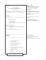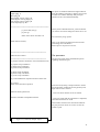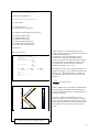
1
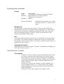
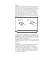
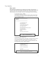
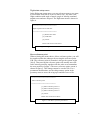
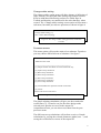
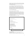
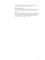
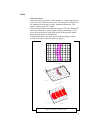
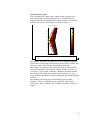
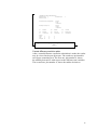
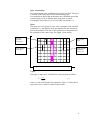
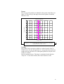
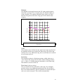
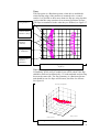
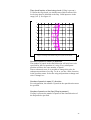
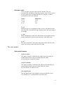
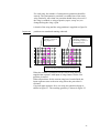
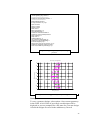
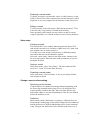
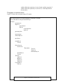
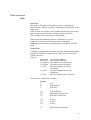
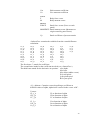
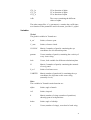
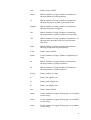
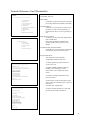
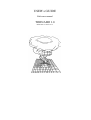
USER’s GUIDE
Reference manual
TORNADO 1.0
RELEASE 2.3 2001-01-31
REGARDING THIS DOCUMENT .....................................................................................................................4
FORMAT ............................................................................................................................................................... 4
BACKGROUND ......................................................................................................................................................4
AIM ......................................................................................................................................................................4
COPYRIGHT INFORMATION ...................................................................................................................................4
INTRODUCTION TO TORNADO .....................................................................................................................4
THE PROGRAM......................................................................................................................................................4
Methods. ..........................................................................................................................................................5
Applications.....................................................................................................................................................5
Cautions...........................................................................................................................................................6
QUICK-START .....................................................................................................................................................6
HOW-TO ............................................................................................................................................................... 6
Start Tornado...................................................................................................................................................6
Load a geometry ..............................................................................................................................................6
Load a state .....................................................................................................................................................6
Calculate a solution.........................................................................................................................................6
View results......................................................................................................................................................6
USER INTERFACE ..............................................................................................................................................7
MENU SYSTEM......................................................................................................................................................7
Tornado Main Menu (TMM)............................................................................................................................7
Aircraft geometry setup menu..........................................................................................................................7
Flight state setup menu....................................................................................................................................8
Move reference point. ......................................................................................................................................8
Change rudder setting. ....................................................................................................................................9
Processor access..............................................................................................................................................9
Post-processing, Result/Plot functions ..........................................................................................................10
Keyboard access ............................................................................................................................................10
About / Release Info.......................................................................................................................................11
EXIT............................................................................................................................................................... 11
PLOTS .................................................................................................................................................................12
Geometry plots...............................................................................................................................................12
Simple solution plots......................................................................................................................................13
Central difference solution plots....................................................................................................................14
Sweep plots. ...................................................................................................................................................15
OUTPUT FILES.....................................................................................................................................................16
DESIGN FEATURES..........................................................................................................................................16
CO-ORDINATE SYSTEM. ......................................................................................................................................16
MAIN WING REFERENCE. ....................................................................................................................................16
WINGS................................................................................................................................................................ 16
PARTITIONS. .......................................................................................................................................................16
PANELS...............................................................................................................................................................17
WING FEATURES.................................................................................................................................................17
Apex coordinates. ..........................................................................................................................................18
Span. ..............................................................................................................................................................18
Taper..............................................................................................................................................................18
Sweep.............................................................................................................................................................19
Camber. .........................................................................................................................................................19
Dihedral.........................................................................................................................................................20
Number of panels in chord (X) direction. ......................................................................................................22
Number of panels in span (Y) direction. ........................................................................................................22
Number of panels on the flap (If flap is present.) ..........................................................................................22
REFERENCE UNITS. .............................................................................................................................................23
2
S_ref...............................................................................................................................................................23
c_mac.............................................................................................................................................................23
b_ref............................................................................................................................................................... 23
THE STATE MODEL.........................................................................................................................................23
STATE MODEL FEATURES ....................................................................................................................................23
Angle of attack...............................................................................................................................................23
Angle of sideslip.............................................................................................................................................23
Roll angular rate ...........................................................................................................................................23
Pitch angular rate..........................................................................................................................................24
Yaw angular rate ...........................................................................................................................................24
Air speed ........................................................................................................................................................24
TORNADO FUNCTIONS. .................................................................................................................................24
GEOMETRY SETUP. .............................................................................................................................................24
Creating a model. ..........................................................................................................................................24
Saving a model. .............................................................................................................................................26
Restoring a saved model................................................................................................................................ 27
Editing a model..............................................................................................................................................27
STATE SETUP. .....................................................................................................................................................27
Creating a model. ..........................................................................................................................................27
Saving a model. .............................................................................................................................................27
Restoring a saved model................................................................................................................................ 27
CHANGE CONTROL SURFACE SETTING. ...............................................................................................................27
Specifying control surface. ............................................................................................................................27
Deflection. .....................................................................................................................................................27
PROGRAM EXECUTION CHART..................................................................................................................28
DATA STRUCTURES ........................................................................................................................................29
FILES ..................................................................................................................................................................29
Input files. ......................................................................................................................................................29
Output files. ...................................................................................................................................................29
VARIABLES.........................................................................................................................................................31
Global. ...........................................................................................................................................................31
Main...............................................................................................................................................................31
Input variables...............................................................................................................................................33
Flight condition variables..............................................................................................................................35
FUNCTION FILES. ................................................................................................................................................35
SAMPLE RUN.....................................................................................................................................................38
Starting up. ....................................................................................................................................................38
The main menu ..............................................................................................................................................38
The Geometry menu.......................................................................................................................................39
Post-processor. ..............................................................................................................................................40
Flight state setup ...........................................................................................................................................40
The processor ................................................................................................................................................41
REFERENCES: ...................................................................................................................................................43
LICENSE & COPYRIGHT INFORMATION: ................................................................................................ 44
TORNADO REFERENCE CARD (DETACHABLE) .....................................................................................45
3
Regarding this document
Format
Author:
Title:
Publisher:
Published:
Tomas Melin
User’s guide and reference manual for Tornado.
Royal Institute of Technology (KTH),
Department of aeronautics.
2000-12
Release information:
Substitutes the document “User’s guide
to Tornado, release 2.1, 2000-10, same
author.
Background
This document is a part of the master thesis ”A Vortex Lattice MATLAB
Implementation for Linear Aerodynamic Wing Applications” by Tomas Melin
written at the Aerodynamics department during 1999-2000. This is the user's
guide for the Matlab program ”Tornado”, which is part of the thesis, and
contains a description of the program.
Aim
It is the aim of this document to provide a user’s guide and a reference manual
for Tornado. The contents should give instructions on how to use and develop
the program. Also, the inner structure of Tornado is explained and the course of
program execution is shown.
Copyright information
This document as well as the program “Tornado” is distributed according to the
GNU-Open license protocol.
Introduction to Tornado
The program.
Tornado is a 3D-vortex lattice program with flexible wake. It may
be used for a variety of tasks that require the Tornado's output.
These outputs are: 3D forces acting on each panel, aerodynamic
coefficients in both body and wind axis. Stability derivatives with
respect to angle of attack, angle of sideslip, angular rates and
rudder deflections.
In order to be easily ported, Tornado is written in Matlab. The
required Matlab version is 5.3. Tornado works on any Matlabsupporting platforms. It has been tested for win95,win98, NT4,
Solaris and Mac OS.
Tornado is an open source program, according to GNU.
4
Methods.
Tornado is based on standard vortex lattice theory, stemming from
potential flow theory. The wake coming off the trailing edge of
every lifting surface is flexible and changes shape according to the
flight condition. For example: a rolling aircraft will have a “corkscrew” shaped wake, which will influence the aerodynamic
coefficients. The classical “horse-shoe” arrangement of other
vortex-lattice programs has been replaced with a “vortex-sling”
arrangement. It basically works in the same way as the “horseshoe” procedure with the exception that the legs of the shoe are
flexible and consist of seven (instead of three) vortices of equal
strength. This is shown in figure 1.
Vortex sling on a
panel with flap
Horse shoe on
ordinary panel
Figure 1: The seven-segment vortex sling vs the horse shoe.
The source of the basic theory for the vortex lattice method used in
Tornado has been the book "Computational Fluid Dynamics" by
Moran [1].
To calculate the first order derivatives, Tornado performs a central
difference calculation using the pre-selected state and disturbing it
by a small amount, usually 0.5 degrees.
With the distorting wake, non-linear effects will be visible in some
designs, especially in those where main wing/stabiliser interactions
are important.
Applications.
Tornado is meant to be used primarily in the conceptual design
stage of aircraft construction or in training and education.
Tornado supports multi-wing designs with swept, tapered,
cambered, twisted and cranked wings with or without dihedral.
Any number of wings may be utilised as well as any number of
control surfaces. Canards, flaps, ailerons, elevators and rudders
may be employed. Winglets, fences and engine mounts may also
be incorporated in the design.
5
Cautions.
One of the primary assumptions in the vortex lattice theory is the
small angle of attack. Therefore, caution is advised when
examining large angles as well as large rotational speeds.
No consideration is taken to fuselage effects or to any friction
drag.
Compressibility effects are neglected, as are thickness effects of
the lifting surfaces.
Quick-start
How-to
Start Tornado
Start Matlab, version 4.2 or later.
Connect to the directory containing Tornado.
Start Tornado by typing “Tornado”, and press enter.
Load a geometry
Select option <Aircraft geometry setup>
Select option <load geometry>
Load the example file X-00.mat by typing “X-00” and press enter.
Load a state
Select option <flight state setup>
Select option <load state>
Load the example file a5v10.mat by typing “a5v10” and press
enter.
Calculate a solution
Select option <Processor access>
Select option <Simple solutions calculation>
View results
Select option <Post processor >
Select option <Solution plot, simple state>
6
User Interface
Menu system
Most functions in Tornado may be reached via text menus. The menu that
becomes visible directly at start-up is the main menu. Other menus are the flight
state menu, the solver menu and the result/plot menu. Navigate through the
different menus enter the number of the row containing the desired command.
Tornado Main Menu (TMM)
This version of Tornado is text-based with a menu system. From
the Tornado main menu all of the essential functions in Tornado
may be reached, see fig. 2.
""""""""""""""""""""""""""""""""""""""""""""""""""""""""""
" TORNADO
"
" Main Menu
"
"
"
""""""""""""""""""""""""""""""""""""""""""""""""""""""""""
[1]. Aircraft geometry setup
[2]. Flight state setup
[3]. Move reference point (origin)
[4]. Change rudder setting
[5]. Processor access
[6]. Post processing, Result/Plot functions
[7]. Keyboard access
[9]. About / Release Info
[0]. EXIT
Please enter choice from above:
Figure 2: Tornado Main Menu.
Aircraft geometry setup menu.
From the Aircraft geometry setup menu, you may select to create a
new geometry design, to load a geometry from file, to save a
geometry to file or to edit a geometry currently in memory. The
aircraft geometry setup is shown in figure 3
[1]. Define New Geometry
[2]. Load Geometry
[3]. Edit current geometry
[4]. Save current geometry
[0]. Cancel
Please enter choice from above:
Figure 3: Aircraft geometry setup menu.
7
Flight state setup menu.
In the flight state setup menu, you may select to create a new state,
to load a state from file or to save a state to file. The state is the
flight condition with angle of attack, angle of sideslip rotational
angular rates and true airspeed. The flight state menu is shown in
figure 4.
"""""""""""""""""""""""""""""""""""""""
Input sequence for aircraft state
"""""""""""""""""""""""""""""""""""""""
[1]. Define New State
[2]. Load State
[0]. Cancel
Please enter choice from above:
Figure 4: Flight state menu as shown in Tornado.
Move reference point.
When selecting the menu choice <Move reference point> you will
be transferred into the submenu for moving the reference point.
N.B. The reference point in Tornado is always the system origin
[0,0,0]. Thus moving the reference point will actually move the
entire aircraft geometry together with the wake to accommodate
the new position of origin. <The move reference point> menu is
shown in figure 5. This change cannot be saved to file. For a
permanent modification, use the edit geometry option in the
geometry menu to move the wing apex and then save to file.
"""""""""""""""""""""""""""""""""""""""
Move reference point
"""""""""""""""""""""""""""""""""""""""
[1]. Move reference point in x
[2]. Move reference point in y
[3]. Move reference point in z
[0]. Cancel
Please enter choice from above:
Figure 5: The Move reference point menu.
8
Change rudder setting.
The change rudder setting menu will allow change of deflection of
flaps, ailerons, elevators and other trailing edge control surfaces.
Keep in mind that all deflecting surfaces are called flaps in
Tornado and that they are numbered in the order that they where
created. The <Change rudder setting> menu option will not start a
sub-menu, but rather just ask two questions as shown in figure 6
Change rudder setting [1..]:
New control deflection [deg]:
Figure 6: The change rudder setting questions, as asked in
Tornado.
Processor access
This menu option will open the main solver submenu. From here
you may choose different forms of solutions. See figure 7.
""""""""""""""""""""""""""""""""""""""""""""""""""""
Main Processor menu
""""""""""""""""""""""""""""""""""""""""""""""""""""
[1]. Simple solution calculation. Forces/Coefficients only
[2]. Alpha sweep calculation
[3]. Beta sweep calculation
[4]. Delta sweep calculation
[5]. Roll sweep calculation
[6]. Pitch sweep calculation
[7]. Yaw sweep calculation
[8]. Central difference expansion around current state
[0]. Cancel
Please enter choice from above:
Figure 7: Main processor menu of Tornado.
The simple solution calculation will give you the zeroth order
coefficients (CL, CD and so on) for the entire design at the
selected state. Results are saved in the output file
/output/fmcoeff.mat, you can also access them from the postprocessor menu.
The different sweep calculations will perform a series of simple
calculations by varying the selected parameter (alpha, beta …) and
saving the coefficients as vectors in the output file.
9
(Example: output/Cx_alpha.mat). The parameter delta is the flap
deflection. In this function you must also specify for which rudder
to do the deflection sweep.
You can also get result plots from the post-processor menu.
The central difference calculation option will launch a central
difference calculation in order to get the first order derivatives of
the coefficients. Results are saved in the output/fmfcoeff.mat. As
before you can review the results directly in the post-processor
menu. Rudder derivatives are stored as a vector in the same order
as their corresponding rudders.
Post-processing, Result/Plot functions
In the post-processor menu you can reach the solutions to each
calculation done in the processor menu. However since results are
saved to file after each calculation, a lock-variable will stop you
from plotting old results from previous calculations. To be on the
safe side you may want to delete all files in the /output/ directory
when starting a new design.
The post-processor menu is shown in figure 8.
""""""""""""""""""""""""""""""""""""
Tornado plotting functions:
""""""""""""""""""""""""""""""""""""
[1]. Clear plots
[2]. Geometry plot
[3]. Solution plot, simple state
[4]. Solution Central difference expansion
[5]. Solution Alpha sweep
[6]. Solution Beta sweep
[7]. Solution Delta sweep
[8]. Solution Roll speed sweep
[9]. Solution Pitch speed sweep
[10]. Solution Yaw speed sweep
[0]. BACK
Enter type of plot:_
Figure 8: The post-processor menu of Tornado.
Keyboard access
Selecting the <keyboard access> option will give you a “>>”
prompt in the workspace, this might come in handy if you want to
10
check some variables during execution. Return to the Tornado
main menu by typing “return” and press enter.
About / Release Info
The about / release info menu option will, when selected, give you
the release info with changes in design since the last update.
EXIT
Terminates Tornado, some variables will remain in memory, so be
sure to clear these if running your own modules afterwards. If you
have run the solver, the result variables will be available in the
output directory and are called "*.mat" files.
11
Plots
Geometry plots
When you select the option <draw geometry> in the postprocessor
menu, Tornado will draw three plots. The first plot is a 2D-plot of
the planform with layout of wings, partitions and panels. This
figure is drawn in the XY- plane.
The second plot shows the planform layout in 3D. The “Rotate3D”
function is enabled so you can grab the figure and rotate it. This
plot will also show the collocation points of the panels with the
panel normals drawn as dashed lines.
The third plot shows the panel layout with the trailing vortices
visible. All of these plots are shown in figure 9.
1.5
1
0.5
0
-0.5
-1
-1.5
-1.5
-1
-0.5
0
0.5
1
1.5
2
2.5
3
W ing z -c oord
3-D W ing c onfiguration
0.2
0
-0.2
-0.4
-0.6
-0.8
3
2
1
0
4
3
2
-1
1
0
-2
-1
W ing y -c oord
-2
-3
W ing x -c oord
-3
3-D W ing c onfiguration
W ing z -c oord
4
2
0
-2
3
2
1
0
8
-1
6
-2
W ing y -c oord
4
2
-3
0
W ing x -c oord
Figure 9: The three geometry plots.
12
Simple solution plots
The <Solution plot, simple state> option in the post-processor
menu will when selected yield plots 4 to 7. Plot number four
displays the delta cp distribution across the aircraft. A colour bar
indicates the values. An example is shown in figure 10
Delta c p dis tribution
0.8
1.5
0.7
1
0.6
0.5
0.5
0
0.4
-0.5
0.3
-1
0.2
-1.5
0.1
0
0.5
1
Figure 10: Delta cp distribution on wing, alpha =5 degrees.
Plot number five shows the panel force's Z-component displayed
as an arrow on each panel. As the arrow starts in the xy-plane, this
plot is the clearest for designs with moderate dihedral.
Plot number six shows the wing vorticity as an elevated surface
above the planform. This plot will only be useful, or accurate, if
you have a “convex hull” geometry. Otherwise all points within
the design’s hull which are not part of the geometry (e.g. area
between wing and stabilizer) will be displayed with an interpolated
vorticity.
Plot number seven will present calculation results as hard
numbers. These are loaded from the output file “fmcoeff.m”,
where more data is available. An example of the plot is shown in
figure 11.
13
TO RN A DO CA LA CU LA TIO N RE S ULTS
Referenc e area:
3
Referenc e c hord:
1
Referenc e s pan:
Net W ind forc es (Lift D rag S ide):
4
66. 1459
3.7302
-1.3687e-015
Net B ody forc es (Z X Y ):
66. 2193
-2.0489
-1.3687e-015
CL
0.35998
CZ
0.36038
Cm
-0.21026
CD
0.020301
CX
-0.011151
Cn
5.2632e-019
CY
-7.4487e-018
CC
-7.4487e-018
Cl
-3.8518e-018
S TA TE :
alpha:
5
P:
bet a:
0
Q:
0
R:
0
A irs peed: 10
0
Figure 11: Text output for a simple solution, in Tornado
plot 7.
Central difference solution plots.
After a central difference expansion calculation is made, the results
may be viewed in the post-processor. The results are presented in
two figures containing text. The first one, plot number 8, shows
the stability derivatives with respect to the different state variables.
The second one, plot number 9, shows the rudder derivatives.
14
Sweep plots.
When a sweep calculation has been performed in the <processor
access> menu results can be reviewed using the < Solution Alpha
sweep>, or any other type of sweep that has been performed, from
the post-processor.
All of the sweep plots will yield a figure with six subplots. Each of
these subplots will show a coefficient as a function of the selected
sweep parameter.
An example of a sweep plot is shown in figure 12.
Coeffic ient dependenc y on alpha
x 10
0.4
-17
0
0.3
Cl
CL
-0.5
0.2
-1
0.1
0
-1.5
0
0.05
0.1
0
0.05
A lpha [rad]
0.1
A lpha [rad]
0.015
0
-0.02
CD
Cm
0.01
-0.04
0.005
-0.06
0
-0.08
0
0.05
0.1
0
A lpha [rad]
x 10
0.05
-19
0.1
A lpha [rad]
1
0
Cn
CY
0.5
0
-0.5
-10
-1
0
0.05
A lpha [rad]
0.1
0
0.05
0.1
A lpha [rad]
Figure 12: Solutions plot of an alpha sweep calculation.
Jagged curves are due to large magnification
15
Output files.
Tornado will produce a number of files containing the output from the different
kinds of calculations. Regarding the contents of these files, please see the
chapter on data structures.
The output files are located in the /output/ directory and they are:
ac.mat
A copy of the geometry used for the
last solution
fmcoeff.mat
Results of a simple state calculation.
Fmfcoeff.mat
Results of a central difference
expansion.
Cx_alpha.mat
Results of an alpha sweep.
The other sweep results follow the same pattern, and are called
Cx_beta, Cx_P and so on.
Design features.
Co-ordinate system.
Tornado uses a Cartesian coordinate system with the X-axis along the aircraft
body, increasing aft. The Y-axis is aligned positive out through the starboard
wing when no dihedral is present. The Z-axis is right-hand perpendicular to the
X- and Y-axis. I.e. positive “upwards”. When the dihedral is 90 degrees (as for a
fin) the span is fully aligned in the Z-positive direction.
Main wing reference.
The first wing entered is considered to be the main wing. The root chord of the
main wing defines the direction of the X-axis
Wings.
In TORNADO, every flat surface is considered as a wing, this means that there
are no differences in input or calculation between main wing, stabiliser or fin.
To create both the starboard and the port sides of the main wing, tick “wing is
mirrored”. Do the same for the stabiliser. As for the fin, don’t use the symmetry
setting but set the dihedral angle to 90 degrees. This procedure will give you one
wing half with its span directed in the Z-direction.
Partitions.
Every lifting surface such as wing, fin and so on is composed of a number of
partitions. The simplest wing contains only one partition while a more complex
one may have five or more. In each partition the wing design features are
constant. Examples are sweep and taper ratio. Exceptions are twist and camber
which have to be defined with inner and outer values for the first partition of a
wing. Succeeding partitions take on the outer feature of the previous element as
their inner feature to assure continuity along the wing's span. Thereby, elements
are numbered outwards.
16
Panels.
The panels are the small four-corned elements that build up each partition. No
special input is needed to define their shape, as this is auto generated once the
number of panels in the chord-wise and span-wise directions have been entered.
In the current version of Tornado the panels are evenly distributed on the
partitions. For reference, panels are numbered from the leading edge backwards
in row by row outwards. See figure 13
3-D W ing c onfiguration
2
1.8
1.6
Panel number
W ing y -c oord
1.4
1.2
1
4
0.8
5
0.6
0.4
0.2
1
2
3
0
-0.5
0
0.5
1
1.5
W ing x -c oord
Figure 13: Panel layout for a one partition wing.
Three panel chord wise and three panels semi-spanwise.
Wing features.
Each wing has special features, which define the shape of the wing. During the
geometry setup these are the inputs needed for each partition:
Apex coordinates.
Span.
Taper.
Sweep.
Camber.
Dihedral.
Twist.
Symmetry.
Root chord. (One per wing.)
Flaps.
Flap symmetry. (If flap is present.)
Flap chord in parts of root chord. (If flap is present.)
Number of panels in chord (X) direction.
Number of panels in span (Y) direction.
Number of panels on the flap (If flap is present.)
17
Apex coordinates.
For each wing the apex coordinates have to be specified. The apex
is located at the first partition root chord leading edge
It is important to know that all moments are calculated around the
system origin (0,0,0) so that the main wing apex is placed
accordingly (most often in [-0.25,0,0] if the root chord is 1).
Span.
The span you are required to enter is the semispan of the partition
in question, i.e. the distance from the innermost to the outermost
part of the partition. The sum of the semispans of the partitions is
the semispan of the entire wing. See figure 14 for details.
Second
partition
semi-span
2
Wing semispan
1.5
1
0.5
First partition
semi-span
Wing span &
Reference
span b_ref
0
-0.5
-1
-1.5
-2
-2
-1.5
-1
-0.5
0
0.5
1
1.5
2
2.5
3
Figure 14: The semispans of the partitions and the wing.
Taper.
The taper or taper ratio, is defined for each partition as follows:
couter
(1)
cinner
where c is the local chord of the partitions. Figure 13 above has a
taper ratio of 0.5, which is visible in the picture.
T=
18
Sweep.
The sweep of the partition is defined for the quarter chord line (see
figure 15) The sweep is the angle between the quarter chord line
and the Y-axis.
3-D W ing c onfiguration
2
1.5
1
W ing y -c oord
0.5
0
-0.5
-1
-1.5
-2
-2
-1.5
-1
-0.5
0
0.5
1
W ing x -c oord
1.5
2
2.5
3
Figure 15: Sweep of division is 0 degrees, the quarter chord line
is perpendicular to the Y-axis
Camber.
The camber lines currently available are taken from the NACAXXXX series. For the first partition of a wing, both inner and outer
camber must be specified. For subsequent partitions only the outer
camber is needed.
Note for advanced users: The slope is calculated in the function
“slope.m”. To use other airfoils, this is the function to edit.
19
Dihedral.
The dihedral is the angle between the XY-plane and the quarter
chord line (see figure 16). Currently only one dihedral angle per
wing is possible. For multiple dihedral wings, please use more
than one wing and set the outer wing apex to fit with the inner
wing tip.
3-D W ing c onfiguration
1.5
1
W ing z -c oord
0.5
0
-0.5
-1
-1.5
-2
1.5
1
0.5
0
-0.5
W ing y -c oord
-1
-1.5
Figure 16:Dihedral is 15 degrees, panel normals are the eight unitlength lines.
Twist.
The partition twist is defined as the angle between the tip chord of
the partition and the root chord of the main wing (The first wing
entered). For every additional wing, the root twist has to be entered
as well as the tip twist.
Symmetry.
The symmetry option is a Boolean operator, which when set as
“true” mirrors the wing in the XZ plane. When editing geometry,
true =1, false =0. Usually symmetry should be set for main wing
and stabiliser, but not for the fin.
Root chord. (One per wing.)
The root chord has to be entered for each wing. For a multiple
partition wing, every additional partition after the first will have
their root chords defined by the first partition root chord and taperratio (see section on taper). This is done automatically.
20
Wing number 1
Flaps.
The flap option is a Boolean operator, when this is enabled the
whole trailing edge of the partition is assumed to be a control
surface. It is possible to have more than one flap per wing, but this
requires that the wing contain at least as many partitions as flaps.
The flaps are numbered in the order they are defined, see figure 17.
2
Control surface
number 1 (Flap)
1.5
1
Control surface
number 2.
(Aileron)
0.5
0
-0.5
Wing number
2. (Stabilizer)
-1
-1.5
-2
-0.5
0
0.5
1
1.5
2
2.5
3
3.5
4
Figure 17: Double wing design, with three flaps (control
surfaces)
Flap symmetry. (If flap is present, and wing symmetry is set).
If symmetry for the wing is enabled, you will be asked if the flap
should be deflected symmetrically, i.e. both starboard and port flap
down at the same time. The flap symmetry is a Boolean operator
and should be true for flaps and elevators, but false for ailerons.
See figure18.
3-D W ing c onfiguration
2
1
W ing z -c oord
Control surface
number 3.
(Elevator)
0
-1
3
2
-2
2
1
0
1
0
-1
-1
-2
W ing x -c oord
W ing y -c oord
Figure 18: Asymmetrical flap, deflected 20 degrees.
21
Flap chord fraction of local wing chord. (If flap is present.)
To define the flap chord, you should enter which fraction of the
local wing chord is allocated to the flap. Valid inputs are in the
range [0 to 1]. See figure 19
2
1.5
1
0.5
0
-0.5
-1
-1.5
-2
-1.5
-1
-0.5
0
0.5
1
1.5
2
2.5
3
Figure 19: Flap with chord being 0.25 of the local chord.
Number of panels in chord (X) direction.
The number of panels in the chord direction will only have to be
specified for the first partition of a wing. Every subsequent
partition will have the same number of panels.
Note to advanced users: It is possible to change this value for
subsequent partitions of a wing. To do so, use the <Edit> function
in the geometry menu. Select the wing and partition to change and
select <change nx>.
Number of panels in span (Y) direction.
For each partition, the number of panels in the span direction must
be specified.
Number of panels on the flap (If flap is present.)
If a flap is present, the number of panels in the chord direction of
the flap must be specified.
22
Reference units.
There are three reference units used in Tornado. They are
automatically calculated during the geometry setup. If you want to
use any other value you must edit the file config.m, in which
instructions for this are included.
Name:
S_ref.
c_mac
b_ref
Dimension:
[L^2]
[L]
[L]
S_ref
Reference area, is by default the sum of areas of all panels on the
first wing The first defined wing considered to be the main wing of
the design.
c_mac
Mean aerodynamic chord, is by default the area-weighed average
mean aerodynamic chord of each partition on the main wing.
b_ref
The sum of partition semi-spans of the main wing, and twice this
value if the wing is mirrored in the XZ-plane.
The state model
State model features
Angle of attack
The angle of attack is defined as the angle of the oncoming airstream and the main wing root chord in the XZ-plane.
By convention it is denoted “alpha”.
Angle of sideslip
The angle of sideslip is defined as the angle of the oncoming airstream and the main wing root chord in the XY-plane.
By convention it is denoted “beta”.
Roll angular rate
The roll angular rate is the angular velocity around the X-axis.
It is denoted as “P” and should be entered in rad/s
23
Pitch angular rate
The pitch angular rate is the angular velocity around the Y-axis.
It is denoted as “Q” and should be entered in rad/s
Yaw angular rate
The yaw angular rate is the angular velocity around the Z-axis.
It is denoted as “R” and should be entered in rad/s
Air speed
The air speed is needed to calculate forces and moments. It is
denoted “AS” and should be entered in meters/second.
Tornado functions.
Geometry setup.
Creating a model.
The creation of a new aircraft model is initiated by selecting
<create new geometry> in the geometry menu. This will initiate a
sequence of questions regarding the geometry of the new aircraft.
First the number of wings in the new design should be entered.
Wing in this context means every coherent surface producing lift,
e.g. main wing, stabiliser or vertical fin. For a GA-aircraft these
three would constitute the 3 wings to enter.
For each wing, the input of necessary wing features will be
requested. This will be done in a nested loop, one partition after
another, running down each wing. Please see the wing features
chapter for reference to these inputs.
24
For each wing, the number of semispanwise partitions should be
entered. The semispanwise partition is a subdivision of the entire
wing. Basically, more than one partition should always be used if
the wing is cranked, or wing properties (taper, sweep etc.) are
changed along the wing‘s span.
A sketch of the wing and the wing partition is supplied as figure 20
Important:
partitions are numbered running outboard.
Wing with one
partition, sweep 10
deg, taper 0.5
Wing with two
partitions, sweeps 0
and 20 degs, taper 0.5
on both divisions.
3-D W ing c onfiguration
3-D W ing configuration
2
2
1.8
1.8
1.6
1.6
1.4
1.2
W ing y-coord
W ing y -c oord
1.4
1
0.8
1.2
1
0.8
0.6
0.6
0.4
0.4
0.2
0.2
0
0
-0.5
0
0.5
1
W ing x -c oord
1.5
-0.5
0
0.5
1
1.5
W ing x-coord
Figure 20. Wing and semi-spanwise partitions.
When the number of partitions for the current wing has been
supplied the sequence with input of wing features for the first
partition is started.
When all partitions for the current wing have been defined, the
input sequence turns to the next wing where the procedure is
repeated.
A typical input sequence for a one-wing one-partition design is
shown in figure 21. The resulting geometry is shown in figure 22
25
************************************
* Data regarding wing number: 1
************************************
Number of semispanwise divisions: 1
******************************
Data regarding division1
Is wing mirrored in xz [1 0]: 1
Apex x-coord: 0
Apex y-coord: 0
Apex z-coord: 0
Root chord: 1
Base chord airfoil nr: 0
Wing dihedral [deg]: 0
Number of vortices chordwise: 3
Number of vortices semispanwise: 4
Span of division: 2
Taper ratio: .5
Outboard airfoil nr: 0
1/4 Chord line Sweep [deg]: 20
Outboard 1/4 Chord twist [deg]: 0
Is division flapped [1 0]:1
Flap chord in parts of root chord (0..1): 0.2
Number of chordwise vorticies on flap: 2
Does control deflect symetrically [1 0]:1
Figure 21. Typical input sequence for a wing
partition.
3-D W ing c onfiguration
2
1.5
1
W ing y -c oord
0.5
0
-0.5
Figure 5. Result of input, when using
Plot functions / geometry plot
-1
-1.5
-2
-1.5
-1
-0.5
0
0.5
1
1.5
2
2.5
3
W ing x -c oord
Figure 22: Resulting geometry from inputs in figure 21.
Saving a model.
To save a geometry design, select option <Save current geometry>
in the GSM. A list of files of previously saved designs will be
displayed as you are prompted for a file name for your new design.
All aircraft designs are saved in the subdirectory /aircraft
26
Restoring a saved model.
To load a previously saved model, select <Load Geometry> in the
GSM. A list of files of the contents of the aircraft/ directory will be
displayed as you are prompted for the filename of the file to load.
Editing a model.
To edit a model, choose the option “Edit current geometry”. This
will work only if a geometry is loaded in the memory.
In the geometry editor menu you may choose to add or remove
wings or partitions or to edit the features of one or more partitions.
State setup.
Creating a model.
The state model is less complex than the geometric model. The
state model consists of six variables: Alpha, beta, roll-, pitch- and
yaw-angular rates as well as airspeed.
To create a new state model you must have a defined geometry
onto which the state model should be applied.
Select the <state setup> option in the main menu, continue with
the new state option. Enter the state model parameters as you are
prompted for them.
Saving a model.
In the state menu, select <Save State>. The state model will be
saved as a “*.mat” file in the data/ directory.
Restoring a saved model.
In the state menu, select load state. A list of previously defined
state models is shown.
Change control surface setting.
Specifying control surface.
Control surfaces are numbered running outboard beginning with
the first wing (normally main wing). For a GA design the first
control surface would be the flaps, the second the ailerons, the
third either rudder or elevator depending on if the fin was defined
before the stabiliser or not.
Deflection.
Input control surface deflection is in degrees. All hinge lines are
located at the leading edge of the rudder. Hinge lines run outboard
and the deflection is defined right-hand positive for the starboard
wing. The port side deflection is also defined in the same way if
27
rudder deflection symmetry is not selected, and the opposite if
rudder deflection symmetry is selected (i.e. both flaps deflect
downwards).
Program execution chart.
Figure 23 shows the execution chart of Tornado.
The main function is invoked using the command “tornado”
Every tab shows a deeper function layer
main.m
questions.m
inpt12.m
questions.m
tedit.m
geosetup14.m
gplot.m
geosetup14.m
statesetup.m
wakesetup2.m
specfun.m
setrudder.m
Trot.m
Solverloop.m
Solver4.m
Dnwash.m
Tcros.m
Tnorm.m
Setboundary.m
Setrudder.m
Trot.m
Tplot.m
Gplot.m
Rplot.m
Splot1.m
Splot2.m
Copyright.m
Intro.m
Figure 23: Tornado execution chart.
28
Data structures
Files
Input files.
Input files to Tornado are the geometry files, containing the
aircraft design, and the state files, containing the description of the
flight state.
None of these are needed to run Tornado the first time, but exist so
that you may save and retrieve complex designs from disc.
The variables of the input files are listed below.
When using the standalone function <diffbatch.m> you are
required to specify the files needed in the computation.
Diffbatch.m performs the central difference calculation in batch
mode.
Output files.
A number of output files are produced by the different calculations
possible in Tornado’s main processor. They are all saved in the
/output/ directory
They are:
fmcoeff.m from simple solution.
fmfcoeff.m from central difference.
Cx_alpha.m from alpha sweep calculation.
Cx_beta.m from beta sweep calculation.
Cx_P.m
from roll angular rate sweep
calculation.
Cx_Q.m
from pitch angular rate sweep
calculation.
Cx_R.m
from yaw angular rate calculation.
<Fmcoeff.m> contains the variables
Scalars
L
D
C
Lift
Induced drag
Side force
CL
CD
CC
Lift coefficient
Induced drag coefficient
Side force coefficient
CX
CY
CZ
X-force
Y-force
Z-force
Cl
Roll moment coefficient
29
Cm
Cn
Pitch moment coefficient
Yaw moment coefficient
Vectors
F
M
Body force vector
Body moment vector
Matrices
FORCE
Panel force vector (Force on each
panel)
MOMENTS Panel moment vector (Moments on
origin caused by panel forces)
Cp
Panel coefficient of pressure matrix
<fmfcoeff.m> contains the variables from the central difference
calculation.
CC_P
CC_Q
CC_R
CC_a
CC_b
CC_d
CD_P
CD_Q
CD_R
CD_a
CD_b
CD_d
CL_P
CL_Q
CL_R
CL_a
CL_b
CL_d
CX_P
CX_Q
CX_R
CX_a
CX_b
CX_d
CY_P
CY_Q
CY_R
CY_a
CY_b
CY_d
CZ_P
CZ_Q
CZ_R
CZ_a
CZ_b
CZ_d
Cl_P
Cl_Q
Cl_R
Cl_a
Cl_b
Cl_d
Cm_P
Cm_Q
Cm_R
Cm_a
Cm_b
Cm_d
Cn_P
Cn_Q
Cn_R
Cn_a
Cn_b
Cn_d
The first letter, C, stands for coefficient.
The second letter stands for the coefficient involved (see <fmcoeff.m>)
The third letter stands for the derivative in question: a for alpha.
b for beta.
d for delta (rudder vector)
P for roll speed.
Q for pitch speed.
R for yaw speed.
<Cx_alpha.m> Contains vectors describing a coefficient at
different values of alpha, alpha itself is stored in the vector “affa”.
Vectors:
CL_f_a
CD_f_a
CC_f_a
CL as function of alpha
CD as function of alpha
CC as function of alpha
Cl_f_a
Cm_f_a
Cn_f_a
Cl as function of alpha
Cm as function of alpha
Cn as function of alpha
30
CX_f_a
CY_f_a
CZ_f_a
CX as function of alpha
CY as function of alpha
CZ as function of alpha
Affa
The vector containing the different
values of alpha.
The other output files <Cx_(parameter)> contains the coefficients,
as a function of the parameter used in its name, just like Cx_alpha.
Variables.
Global.
The global variables in Tornado are:
b_ref
Scalar, reference span.
C_mac
Scalar, reference chord.
COLLOC
Matrix (3xnumber of panels) containing the xyz
coordinates for all collocation points
gamma
Vector (number of panels) containing the vorticity of
every vortex sling.
lock
Vector, lock-variable for different calculations/plots
N
Matrix (3xnumber of panels) containing the normals
of every panel.
S_ref
Scalar of reference area.
VORTEX
Matrix (number of panelsx8x3) containing the xyz
coordinates for all points on the vortex sling
(normally 8 or 6).
Main.
The variables in Tornado's main function are:
alpha
Scalar, angle of attack.
AS
Scalar, airspeed.
b
Matrix (number of wings x number of partitions)
showing span of each partitions.
betha
Scalar, angle of sideslip.
c
Vector (number of wings), root chord of each wing.
31
call
Scalar, status variable.
dihed
Matrix (number of wings x number of partitions)
showing dihedral of each partitions.
fc
Matrix (number of wings x number of partitions)
showing flap chord in parts of partitions chord.
flapped
Matrix (number of wings x number of partitions)
showing if partition is flapped.
fnx
Matrix (number of wings x number of partitions)
showing number of panels chordwise on each flap.
foil
Matrix (number of wings x number of partitions x 2)
showing inner and outer airfoil of each partition,
inner first
fsym
Matrix (number of wings x number of partitions)
showing if flaps deflect symmetrically
Loop
Scalar, status variable.
nelem
Vector (number of wings), number of partitions per
wing.
nx
Matrix (number of wings x number of partitions)
showing number of panels chordwise.
ny
Matrix (number of wings x number of partitions)
showing number of panels spanwise.
nwing
Scalar, number of wings
P
Scalar, roll angular rate.
Q
Scalar, pitch angular rate
R
Scalar, yaw angular rate.
stat
Scalar, status variable
startx
Vector (number of wings) showing apex x-coordinate
of each wing.
starty
Vector (number of wings) showing apex y-coordinate
of each wing.
startz
Vector (number of wings) showing apex z-coordinate
of each wing.
32
SW
Matrix (number of wings x number of partitions)
showing sweep of each partition.
symmetric
Vector (number of wings) showing symmetric state
(1 or 0) of each wing.
T
Matrix (number of wings x number of partitions)
showing taper of each partition.
TW
Matrix (number of wings x number of partitions x 2)
showing inner and outer twist of each partitions,
inner first.
void
Scalar, status variable.
XYZ
Matrix (number of panels x 5 x 3) showing xyz
coordinates for every corner of each panel.
Input variables
All of these are variables in Toprnados main function. Some are
needed to create a geometry and these are saved in the geometry
input files in the "aircraft" directory. They are:
b
c
Matrix (number of wings x number of partitions)
showing span of each partitions. Figure 24 shows the
layout of the b matrix, which is representative for all
geometry matrices.
figure 24: Span matrix layout
33
Vector (number of wings), root chord
of each wing.
dihed
Matrix (number of wings x number of partitions)
showing dihedral of each partition. In the current
release (1.10) of Tornado, the dihedral must be
constant along the entire wing.
fc
Matrix (number of wings x number of partitions)
showing flap chord in part of the local partition
chord.
flapped
Matrix (number of wings x number of partitions)
showing if partition is flapped. Boolean (1 or 0).
fnx
Matrix (number of wings x number of partitions)
showing number of panels chord-wise on each flap.
foil
Matrix (number of wings x number of partitions x 2)
showing inner and outer airfoil of each partition,
inner first. Tornado release 1.10 supports flat and
NACA-four digits chamber lines.
fsym
Matrix (number of wings x number of partitions)
showing if flaps deflect symmetrically, Boolean.
nelem
Vector (number of wings), number of partitions per
wing.
nx
Matrix (number of wings x number of partitions)
showing number of panels chordwise.
ny
Matrix (number of wings x number of partitions)
showing number of panels spanwise.
nwing
Scalar, number of wings
startx
Vector (number of wings) showing apex x-coordinate
of each wing.
starty
Vector (number of wings) showing apex y-coordinate
of each wing.
startz
Vector (number of wings) showing apex z-coordinate
of each wing.
SW
Matrix (number of wings x number of partitions)
showing sweep of each partition. In radians.
34
symmetric
Vector (number of wings) showing symmetry state
Boolean (1 or 0) of each wing.
T
Matrix (number of wings x number of partitions)
showing taper of each partition.
TW
Matrix (number of wings x number of partitions x 2)
showing inner and outer twist of each partition, inner
first.
Flight condition variables
These are the variables needed in a state file:
alpha
Scalar, angle of attack.
AS
Scalar, airspeed.
betha
Scalar, angle of sideslip.
P
Scalar, roll angular rate.
Q
Scalar, pitch angular rate
R
Scalar, yaw angular rate.
Function files.
config
Configuration function for different variables, i.e using other than
standard S_ref.
cutline
Not used. For debugging only.
diffbatch
A batch program taking the filename of an aircraft geometry file
and a state file as input. Producing a central difference expansion.
dnwash15:
Function calculating the aerodynamic influence of every vortex
sling on every panel.
drawhinge: Calculates the forward corners of a flap and draws a line in
between, the hinge line.
geometry17: Calculates the corner points, vortex points, normals and
collocation points of each panel.
geosetup14: Calculates the geometry of the wings and partitions, calls
geometry to do the panels.
35
gplot
Plots the geometry of the design, figures 1- 3
inpt12
Input function to get all geometry variables.
Intro
Displays release info and startup-screen.
lemmabatch: Experimental function, not used in Tornado but please examine
further.
main:
Current main function of Tornado.
normals4:
Calculates the normals of each panel.
questions:
Most user interface questions are collected here.
rplot:
Plots various results from a simple state solution.
setboundary3: Calculates the boundary conditions for each panel.
setrudder3: Function that rotates flap coordinates around the hinge.
setup12:
Not used.
slope:
Calculates the angle of normal rotation due to camber.
solver4:
Calculates forces and moments of a design.
solverloop: Loops over solver4 to provide different kinds of solutions.
specfun:
Moves the geometry around in the xyz-space.
splot:
Not used.
splot1:
Plots results of a central difference expansion.
splot2
Plots results of sweep calculations.
statesetup:
Sets up the flight state.
tarea:
Calculates the area of each panel.
tcros:
Cross-product calculation.
tedit:
Edit geometry function.
terror:
Function to produce error messages.
tmesh
Creates the panel cornerpoints.
tnorm
Calculates length of a 3-d vector.
36
tplot
Menu function that calls the different plottingfunctions.
trot3
Rotates one vector around another, used in drawhinge.
wakeplot
Plots the wake in a geometry plot, not currently used, debugging
function.
wakesetup2 Calculates the shape of the wake.
37
Sample Run.
sample>matlab
<MATLAB>
Copyright 1984-1999 The MathWorks, Inc.
Version 5.3.0.10183 (R11)
Jan 21 1999
To get started, type one of these: helpwin, helpdesk, or demo. For
product information, type tour or visit www.mathworks.com.
Figure 25 shows the screen output from a
sample run of Tornado. The planform
comes from Bertin and Smith [2].
Starting up.
In a standard program execution, Matlab
(5.3) should be started in the normal way.
Start Matlab in the directory where the
Tornado files reside
>>
>>Tornado
- program start ****************************************************
*
*
*
*
*
Welcome to Tornado 1.0
*
*
*
*
by: Tomas Melin
*
*
Copyright 1999-2000
*
****************************************************
*
*
*
*
* Release 1.10 Beta 2000-10-02
*
* Fixes since last revision
*
*
divisions change name to partitions for better *
*
clarity.
*
*
*
* Bug in setrudder fixed for multiple wing AC
*
*
Start Tornado by typing "Tornado" then
press enter.
First, some release and copyright
information will be shown before the
Tornado main menu is displayed.
(...)
""""""""""""""""""""""""""""""""""""""""""""""""""""""""""
" TORNADO
"
" Main Menu
"
"
"
""""""""""""""""""""""""""""""""""""""""""""""""""""""""""
The main menu
The main menu shows the available
options in Tornado.
Select 1 to get to the geometry setup menu.
[1]. Aircraft geometry setup
[2]. Flight state setup
[3]. Move reference point (origin)
[4]. Change rudder setting
[5]. Processor access
[6]. Post processing, Result/Plot functions
[7]. Keyboard access
[9]. About / Release Info
[0]. EXIT
Please enter choice from above: 1
Figure 25: Sample screen output
38
""""""""""""""""""""""""""""""""""""""""""""""""""""""""""
The Geometry menu
In the geometry menu, select the option Define
new geometry.
[1]. Define New Geometry
[2]. Load Geometry
[3]. Edit current geometry
[4]. Save current geometry
[0]. Cancel
Please enter choice from above:1
Number of Wings: 1
************************************
*
*
* Data regarding wing number: 1
*
*
************************************
Number of semispanwise partitions: 1
*******************************
* Data regarding partition 1
*
In this sample case, we want to look at a
simple wing.
We start by defining the number of wings: one
<- Number of wings selected.
<- A loop regarding input for the first (and in
this case only) wing starts here.
<- Since it's a simple wing we only need one
partition, selected here.
<- A loop outwards on the first wing starts
here. In this case we only have one partition.
hence it isn't really a loop.
Is wing mirrored in xz [1 0]: 1
NOTE!
Moment calculation will be done around the
system origin. Place main wing apex accordingly.
The wing should be mirrored in the xz plane,
i.e. we want a port and a starboard wing.
Apex x-coord: 0
Apex y-coord: 0
Apex z-coord: 0
Here you define the apex point of the wing, the
origin works fine. More advanced users might
want to put the apex x coordinate in -0.25 for a
wing with a root chord of 1. Doing this would
make all moments to be calculated around the
c/4 point.
Root chord: 2
Base chord airfoil nr: 0
Wing dihedral [deg]: 0
Number of vortices chordwise: 1
Number of vortices semispanwise: 4
Root chord 2, international units (meters)
Flat plate gives airfoil 0.
Dihedral set to zero.
Number of vortices equals number of panels.
Chordwise = x , spanwise= y (if no dihedral is
present)
Span of partition =5 gives tip-to-tip span of 10
as wing is symmetric in xz
A taper of 1 means that the tip chord also is 2
meters.
Wing should be flat at the tip as well.
Sweep the wing c/4 line 45 degrees from the
y-axis
No tip twist.
Trailing edge flap selected.
Selecting a flap chord of 20% of the local
chord.
One chord-wise panel on the flap.
And the flaps should deflect symmetrically on
both port and starboard side, as they would if
they where real "flaps" and not "ailerons".
Span of partition: 5
Taper ratio: 1
Outboard airfoil nr: 0
1/4 Chord line Sweep [deg]: 45
Outboard 1/4 Chord twist [deg]: 0
Is partition flapped [1 0]:1
Flap chord in parts of root chord (0..1): 0.2
Number of chordwise vortices on flap: 1
Does control deflect symmetrically [1 0]:1
Figure 25 (continued): Sample output
39
(Main menu as above)
Tornado plotting functions:
After this input sequence, we return to the
Main menu.
To be sure that the geometry looks the
way we want it, we should plot it. This is
done via the post-processor menu, option
6.
""""""""""""""""""""""""""""""""""""
Select option 6 in the Main menu:
[1]. Clear plots
Post-processor.
""""""""""""""""""""""""""""""""""""
[2]. Geometry plot
[3]. Solution plot, simple state
[4]. Solution Central difference expansion
[5]. Solution Alpha sweep
[6]. Solution Beta sweep
[7]. Solution Delta sweep
[8]. Solution Roll speed sweep
[9]. Solution Pitch speed sweep
[10]. Solution yaw speed sweep
[0]. BACK
Selecting plot option number 2 will plot
the geometry stored in memory.
Enter type of plot:2
3-D W ing configuration
5
4
3
W ing y -c oord
2
1
The plot to the left shows the aircraft
geometry as plotted from the
postprocessor, plot geometry option.
0
-1
-2
-3
-4
-5
-2
0
2
4
6
8
"""""""""""""""""""""""""""""""""""""""
When the plotting functions have finished
drawing the figures, we should be back in
the main menu.
Since the geometry looked as we wanted,
we can continue to the calculations.
Input sequence for aircraft state
Flight state setup
W ing x -c oord
"""""""""""""""""""""""""""""""""""""""
[1]. Define New State
[2]. Load State
[0]. Cancel
Please enter choice from above:1
Before completing any calculations we
must select a flight condition, or flight
state as it is called in Tornado. Go to the
flight state setup menu in Tornado by
selection option number 2 in the main
menu.
In the flight state setup menu, select
option number 1 to define a new state:
Figure 25 (continued): Sample output
40
Alpha [deg]: 5
Beta [deg]: 0
Roll angular velocity [deg/s]: 0
Pitch angular velocity [deg/s]: 0
Yaw angular velocity [deg/s]: 0
True airspeed [m/s]: 10
Six inputs are needed to define the flight condition.
Enter the numbers in degrees or degrees per second.
Tornado uses radians internally and your input
number will be converted automatically.
""""""""""""""""""""""""""""""""""""""""""""""""""""""""
[1]. Save data, then go
[2]. Just go.
Please enter choice from above 2
(Main menu as before.)
When you have defined the state, you'll be asked if
you want to save these settings for future use or not.
We choose the just go option.
Now we are back in the main menu and can start
performing some calculations.
Select option 5 for processor access.
""""""""""""""""""""""""""""""""""""""""""""""""""""
Main Processor menu
""""""""""""""""""""""""""""""""""""""""""""""""""""
[1]. Simple solution calculation. Forces/Coefficients only
The processor
The processor menu shows the different options
regarding calculation types.
[2]. Alpha sweep calculation
[3]. Beta sweep calculation
[4]. Delta sweep calculation
[5]. Roll sweep calculation
[6]. Pitch sweep calculation
[7]. Yaw sweep calculation
[8]. Central difference expansion around current state
[0]. Cancel
Enter choice from above please:1
Solution started, please wait.
Solution available in output/fmcoeff.mat
We'll start off by doing a simple solution to obtain
the aerodynamic coefficients for the geometry and
flight state we have selected.
<-This row shows that the solver has started.
<-This row signals that the calculation is completed,
and where the results are saved.
This transfers us back to the main menu and from
the post-processor menu we can now review the
results as plots.
Figure 25 (continued): Sample output
41
""""""""""""""""""""""""""""""""""""
Tornado plotting functions:
""""""""""""""""""""""""""""""""""""
[1]. Clear plots
[2]. Geometry plot
[3]. Solution plot, simple state
[4]. Solution Central difference expansion
[5]. Solution Alpha sweep
[6]. Solution Beta sweep
[7]. Solution Delta sweep
[8]. Solution Roll speed sweep
[9]. Solution Pitch speed sweep
[10]. Solution Yaw speed sweep
[0]. BACK
Selecting option 3 in the post-processor menu
yields a couple of plots, one being forces in Newton
in both wind and body axis.
Coefficients of forces and moments are also
represented. A glance at the pitching moment
reveals a large nose down moment. This is because
the reference point is located in the origin, where
we put the apex. A better location of the apex
should be somewhere at x=-1 or -2.
Enter type of plot: 3
TO RNA DO CA LA CULA TIO N RE S ULTS
Referenc e s pan:
Referenc e area:
20
Referenc e c hord: 1
Net W ind forc es (Lift Drag S ide):
366.7046
5.9897
9.4369e-016
Net B ody forc es (Z X Y ):
365.8312
-25.9935
10
9.4369e-016
CL
CD
CY
0.29935
0.0048896
7.7036e-019
CZ
CX
CC
S TA TE :
alpha:
5
beta:
0
A irs peed: 10
0.29864
-0.021219
7.7036e-019
P:
Q:
R:
Cm
Cn
Cl
-0.88124
9.9693e-019
2.0301e-018
Having a look at CL, which equals 0.29935 for an
alpha of five degrees, one could easily calculate the
liftslope CL_a. Knowing that the CL at alpha =0
also should be zero (flat plate wing), the lift slope
should be:
0
0
0
CL
= 3.430 [1/rad]
5⋅π
180
Delta c p dis tribution
5
0.35
4
3
0.3
2
There is a difference in the liftslope calculated here
and the liftslope calculated in Bertin & Smith [2]
(3.443), but then again there is a slight difference in
geometry (the flap)
0.25
1
0
0.2
-1
-2
0.15
-3
0.1
-4
A pressure difference coefficient plot is also
displayed, which reveals the panel layout could be
better. The large gradient in pressure from wing to
flap indicates that a larger number of panels should
be used chord wise to get better (more accurate)
results.
-5
0
2
4
6
Figure 25 (continued): Sample output
42
References:
[1]
[2]
Moran.J, Computational Fluid Dynamics, Weily & Sons, 1984.
Bertin.J & Smith,M, Aerodynamics for engineers, 3rd Ed.,Prentice Hall, 1998
43
License & copyright information:
Tornado, a Vortex lattice program for conceptual aircraft design.
Copyright (C) 2000 Tomas Melin
This program is free software; you can redistribute it and/or modify
it under the terms of the GNU General Public License as published by
the Free Software Foundation; either version 2 of the License, or
(at your option) any later version.
This program is distributed in the hope that it will be useful,
but WITHOUT ANY WARRANTY; without even the implied warranty of
MERCHANTABILITY or FITNESS FOR A PARTICULAR PURPOSE. See the
GNU General Public License for more details.
You should have received a copy of the GNU General Public License
along with this program; if not, write to the Free Software
Foundation, Inc., 59 Temple Place, Suite 330, Boston, MA 02111-1307 USA
The Author can be reached by:
Postal mail:
Tomas Melin, Institutionen för flygteknik
Teknikringen 8 5 tr
SE-100 44 Stockholm
SWEDEN
E-mail:
[email protected]
The Royal Institute of Technology (KTH), hereby disclaims all copyright interest in the program
Tornado (a vortex lattice program) written by Tomas Melin.
20 Dec 2000
Arthur Rizzi, Prof.
44
Tornado Reference Card (Detachable)
""""""""""""""""""""""""""""""""""""""""""""""""""""""""""
" TORNADO
"
" Main Menu
"
"
"
""""""""""""""""""""""""""""""""""""""""""""""""""""""""""
[1]. Aircraft geometry setup
[2]. Flight state setup
[3]. Move reference point (origin)
[4]. Change rudder setting
[5]. Processor access
[6]. Post proccessing, Result/Plot functions
[7]. Keyboard access
[9]. About / Release Info
[0]. EXIT
Please enter choice from above:
[1.]
Geometry menu.
[1]. Define New Geometry
[2]. Load Geometry
[3]. Edit current geometry
[4]. Save current geometry
[0]. Cancel
Please enter choice from above:
Shown to the left are the four most important menus
of Tornado. They are:
Main Menu:
From here you may reach all pre- and postprocessing functions available in Tornado.
Geometry Menu:
From here you can choose to create a new
geometry, to edit a current geometry, to
load one from file or to save a geometry to
file.
Main Processor Menu:
From here you may start the computations
that Tornado does.
The simple calculation should be the
primary option when trying out a new
design.
Tornado Plotting Functions Menu:
From here the results from previously done
calculations may be accessed as plots.
Program Execution:
The normal way of performing
computations with Tornado is to:
[5.]
""""""""""""""""""""""""""""""""""""""""""""""""""""
Main Processor menu
""""""""""""""""""""""""""""""""""""""""""""""""""""
[1]. Simple solution calculation. Forces/Coefficients only
[2]. Alpha sweep calculation
[3]. Beta sweep calculation
[4]. Delta sweep calculation
[5]. Roll sweep calculation
[6]. Pitch sweep calculation
[7]. Yaw sweep calculation
[8]. Central difference expansion around current state
[0]. Cancel
Enter choice from above please
1) Define geometry, either load one or
create a new one.
2) Define a flight condition, either by
loading one or creating a new one.
This is done in the "Flight state setup
menu"
3) Perform a simple calculation in the
processor menu.
4) Review the results in the postprocessor
menu, using the "Geometry plot" option as
well as the
"Solution plot, simple state"
[6.]
""""""""""""""""""""""""""""""""""""
Tornado plotting functions:
5) Iterate, change geometry or state, and
perform some sweep calculations
""""""""""""""""""""""""""""""""""""
[1]. Clear plots
[2]. Geometry plot
[3]. Solution plot, simple state
[4]. Solution Central difference expansion
[5]. Solution Alpha sweep
[6]. Solution Beta sweep
[7]. Solution Delta sweep
[8]. Solution Roll speed sweep
[9]. Solution Pitch speed sweep
[10]. Solution yaw speed sweep
[0]. BACK
Enter type of plot:
45