Download C:Documentsin Working_Manuals02Line02.wpd

AQWA™-LIBRIUM
MANUAL
Release 12.0 April 2009
Revision Information
The information in this guide applies to all ANSYS, Inc. products released on or after this date, until superseded by
a newer version of this guide. This guide replaces individual product installation guides from previous releases.
Copyright and Trademark Information
© 2009 Ansys, Inc. All rights reserved. Unauthorized use, distribution or duplication is prohibited
ANSYS, ANSYS Workbench, CFX, AUTODYN, ASAS, AQWA and any and all ANSYS, Inc. product and service
names are registered trademarks or trademarks of ANSYS, Inc. or its subsidiaries located in the United States or
other countries. ICEM CFD is a trademark licensed by ANSYS, Inc.
ABAQUS is a registered trademark of ABAQUS, Inc
Adobe and Acrobat are registered trademarks of Adobe Systems Incorporated
Compaq is a registered trademark of Compaq Computer Corporation
Delphi is a registered trademark of Borland Software orporation
DXF is a trademark of Autodesk, Inc
FEMGV, FEMGEN and FEMVIEW are trademarks of Femsys Limited
FLEXlm and FLEXnet are registered trademarks of Macrovision Corporation
Formula One is a trademark of Visual Components, Inc
GINO is a registered trademark of Bradly Associates Ltd
IGES is a trademark of IGES Data Analysis, Inc
Intel is a registered trademark of Intel Corporation
Mathcad is a registered trademark of Mathsoft Engineering & Education, Inc.
Microsoft, Windows, Windows 2000, Windows XP and Excel are registered trademarks of Microsoft Corporation
NASTRAN is a registered trademark of the National Aeronautics and Space Administration.
PATRAN is a registered trademark of MSC Software Corporation
SentinelSuperPro™ is a trademark of Rainbow Technologies, Inc
SESAM is a registered trademark of DNV Software
Softlok is a trademark of Softlok International Ltd All other trademarks or registered trademarks are the property of
their respective owners.
Disclaimer Notice
THIS ANSYS SOFTWARE PRODUCT AND PROGRAM DOCUMENTATION INCLUDE TRADE SECRETS
AND ARE CONFIDENTIAL AND PROPRIETARY PRODUCTS OF ANSYS, INC., ITS SUBSIDIARIES, OR
LICENSORS. The software products and documentation are furnished by ANSYS, Inc., its subsidiaries, or affiliates
under a software license agreement that contains provisions concerning non-disclosure, copying, length and nature
of use, compliance with exporting laws, warranties, disclaimers, limitations of liability, and remedies, and other
provisions. The software products and documentation may be used, disclosed, transferred, or copied only in
accordance with the terms and conditions of that software license agreement. ANSYS, Inc. and ANSYS Europe,
Ltd. are UL registered ISO 9001:2000 Companies.
U.S. Government Rights
For U.S. Government users, except as specifically granted by the ANSYS, Inc. software license agreement, the use,
duplication, or disclosure by the United States Government is subject to restrictions stated in the ANSYS, Inc.
software license agreement and FAR 12.212 (for non-DOD licenses).
Third-Party Software
The products described in this document contain the following licensed software that requires reproduction of the
following notices.
Copyright 1984-1989, 1994 Adobe Systems Incorporated. Copyright 1988, 1994 Digital Equipment Corporation.
Permission to use, copy, modify, distribute and sell this software and its documentation for any purpose and without
fee is hereby granted, provided that the above copyright notices appear in all copies and that both those copyright
notices and this permission notice appear in supporting documentation, and that the names of Adobe Systems and
Digital Equipment Corporation not be used in advertising or publicity pertaining to distribution of the software
without specific, written prior permission. Adobe Systems & Digital Equipment Corporation make no
representations about the suitability of this software for any purpose. It is provided "as is" without express or
implied warranty.
Microsoft, Windows, Windows 2000 and Windows XP are registered trademarks of Microsoft Corporation
The ANSYS third-party software information is also available via download from the Customer Portal on the
ANSYS web page. If you are unable to access the third-party legal notices, please contact ANSYS, Inc.
Published in the United Kingdom
AQWA™ LIBRIUM User Manual
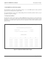
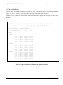
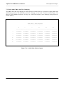
Contents
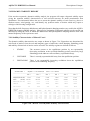
CONTENTS
CHAPTER 1 - INTRODUCTION ................................................................................................................. 8
1.1 PROGRAM INTRODUCTION ........................................................................................................... 8
1.2 MANUAL INTRODUCTION ............................................................................................................. 8
CHAPTER 2 - PROGRAM DESCRIPTION ................................................................................................. 9
2.1 PROGRAM CAPABILITIES .............................................................................................................. 9
2.2 THE COMPUTER PROGRAM ......................................................................................................... 10
CHAPTER 3 - THEORETICAL FORMULATION .................................................................................... 11
3.1 HYDROSTATIC LOADING ............................................................................................................. 12
3.2 MORISON FORCES.......................................................................................................................... 13
3.3 DIFFRACTION/RADIATION WAVE FORCES ............................................................................. 14
3.4 MEAN WAVE DRIFT FORCES ....................................................................................................... 14
3.5 VARIABLE WAVE DRIFT FORCES .............................................................................................. 15
3.6 INTERACTIVE FLUID LOADING .................................................................................................. 15
3.7 STRUCTURAL ARTICULATIONS AND CONSTRAINTS ........................................................... 15
3.8 WIND AND CURRENT LOADING ................................................................................................. 15
3.9 THRUSTER FORCES ....................................................................................................................... 15
3.10 MOORING LINES ........................................................................................................................... 16
3.10.1 Tension and Stiffness for Mooring Lines with No Mass ........................................................... 17
3.10.2 Tension and Stiffness for Catenaries ......................................................................................... 18
3.10.3 Translation of the Mooring Line Force and Stiffness Matrix .................................................... 19
3.10.4 Stiffness Matrix for a Mooring Line Joining Two Structures ................................................... 19
3.11 WAVE SPECTRA............................................................................................................................ 20
3.12 EQUILIBRIUM AND STABILITY ANALYSIS............................................................................ 20
3.12.1 Solution of the Equilibrium Position ......................................................................................... 20
3.12.2 Static Stability Analysis ............................................................................................................. 22
3.12.3 Dynamic Stability Analysis ....................................................................................................... 22
3.13 LIMITATIONS OF THEORETICAL APPLICATIONS ................................................................ 23
CHAPTER 4 - MODELLING TECHNIQUES............................................................................................ 24
4.1 INTRODUCTION .............................................................................................................................. 25
4.2 MODELLING REQUIREMENTS FOR AQWA-LIBRIUM ............................................................ 25
4.2.1 Following an AQWA-LINE Run................................................................................................. 26
4.3 DEFINITION OF STRUCTURE AND POSITION .......................................................................... 28
4.4 STRUCTURE GEOMETRY AND MASS DISTRIBUTION ........................................................... 30
Contains proprietary and confidential information of ANSYS, Inc. and its subsidiaries and affiliates
Page 4 of 122
AQWA™ LIBRIUM User Manual
Contents
4.4.1 Coordinates .................................................................................................................................. 30
4.4.2 Elements and Element Properties ................................................................................................ 30
4.5 MORISON ELEMENTS .................................................................................................................... 30
4.6 STATIC ENVIRONMENT ................................................................................................................ 32
4.6.1 Global Environmental Parameters ............................................................................................... 32
4.7 LINEAR STIFFNESS ........................................................................................................................ 32
4.7.1 Hydrostatic Stiffness .................................................................................................................... 32
4.7.2 Additional Linear Stiffness .......................................................................................................... 32
4.8 WAVE FREQUENCIES AND DIRECTIONS.................................................................................. 33
4.9 WAVE LOADING COEFFICIENTS ................................................................................................ 33
4.10 WIND AND CURRENT LOADING COEFFICIENTS AND THRUSTERS ................................ 34
4.11 THRUSTER FORCES ..................................................................................................................... 34
4.12 CURRENT AND WIND VELOCITIES AND DIRECTIONS ....................................................... 34
4.13 CONSTRAINTS OF STRUCTURE MOTIONS ............................................................................. 34
4.14 WAVE SPECTRA, WIND AND CURRENT SPECIFICATION ................................................... 35
4.15 MOORING LINES ........................................................................................................................... 35
4.15.1 Linear/Non-Linear Elastic Hawsers .......................................................................................... 35
4.15.2 Constant Tension Winch Line ................................................................................................... 36
4.15.3 ‘Constant Force’ Line ................................................................................................................ 36
4.15.4 Composite catenary Line ........................................................................................................... 36
4.16 ITERATION PARAMETERS FOR SOLUTION OF EQUILIBRIUM .......................................... 37
4.16.1 Iteration Limits .......................................................................................................................... 37
4.16.2 Iteration Step Size ...................................................................................................................... 37
4.16.3 Convergence Limits ................................................................................................................... 38
4.17 TIME HISTORY INTEGRATION IN IRREGULAR WAVES (AQWA-DRIFT/NAUT)............. 39
4.18 TIME HISTORY INTEGRATION IN REGULAR WAVES (AQWA-NAUT ONLY) ................. 39
4.19 SPECIFICATION OF OUTPUT REQUIREMENTS ...................................................................... 39
CHAPTER 5 - ANALYSIS PROCEDURE ................................................................................................. 40
5.1 TYPES OF ANALYSIS ..................................................................................................................... 41
5.2 RESTART STAGES .......................................................................................................................... 41
5.3 STAGES OF ANALYSIS .................................................................................................................. 41
CHAPTER 6 - DATA REQUIREMENT AND PREPARATION .............................................................. 43
6.0 ADMINISTRATION CONTROL - DECK 0 - PRELIMINARY DECK .......................................... 44
6.1 STAGE 1 - DECKS 1 TO 5 - GEOMETRIC DEFINITION AND STATIC ENVIRONMENT ...... 44
Contains proprietary and confidential information of ANSYS, Inc. and its subsidiaries and affiliates
Page 5 of 122
AQWA™ LIBRIUM User Manual
Contents
6.1.1 Description Summary of Physical Parameters Input ................................................................... 45
6.1.2 Description of General Format .................................................................................................... 45
6.1.3 Data Input Summary for Decks 1 to 5 ......................................................................................... 45
6.2 STAGE 2 - DECKS 6 TO 8 - THE DIFFRACTION/RADIATION ANALYSIS PARAMETERS.. 46
6.2.1 Description Summary of Physical Parameters Input ................................................................... 46
6.2.2 Description of General Format .................................................................................................... 47
6.2.3 Total Data Input Summary for Decks 6 to 8................................................................................ 47
6.2.4 Input for AQWA-LIBRIUM using the Results of a Previous AQWA-LINE Run ...................... 48
6.2.5 Input for AQWA-LIBRIUM with Results from Source other than AQWA-LINE ..................... 48
6.2.6 Input for AQWA-LIBRIUM with Results from a Previous AQWA-LINE Run and a Source
other than AQWA-LINE ...................................................................................................................... 48
6.3 STAGE 3 - NO CARD IMAGE INPUT - DIFFRACTION/RADIATION ANALYSIS .................. 49
6.3.1 Stage 3 in AQWA-LIBRIUM ...................................................................................................... 49
6.4 STAGE 4 - DECKS 9 TO 18 - INPUT OF THE ANALYSIS ENVIRONMENT............................. 49
6.4.1 Description of Physical Parameters Input.................................................................................... 49
6.4.2 AQWA-LIBRIUM Data Input Summary for Decks 9 to 18. ...................................................... 51
6.5 STAGE 5 - NO INPUT - EQUILIBRIUM ANALYSIS .................................................................... 51
CHAPTER 7 - DESCRIPTION OF OUTPUT............................................................................................. 52
7.1 STRUCTURAL DESCRIPTION OF BODY CHARACTERISTICS ............................................... 53
7.1.1 Properties of All Body Elements ................................................................................................. 53
7.2 DESCRIPTION OF ENVIRONMENT .............................................................................................. 57
7.3 DESCRIPTION OF FLUID LOADING ............................................................................................ 59
7.3.1 Hydrostatic Stiffness .................................................................................................................... 59
7.3.2 Wave Drift Forces........................................................................................................................ 60
7.3.3 Drift Added Mass and Wave Damping ....................................................................................... 61
7.4 DESCRIPTION OF STRUCTURE LOADING ................................................................................ 62
7.4.1 Thruster Forces and Wind and Current Coefficients ................................................................... 62
7.4.2 Structure Constraints ................................................................................................................... 63
7.4.3 Cable/Line Mooring Configurations............................................................................................ 65
7.5 DESCRIPTION OF ENVIRONMENTAL CONDITIONS ............................................................... 67
7.5.1 Wind and Current Conditions (no waves) ................................................................................... 67
7.6 ITERATION PARAMETERS ........................................................................................................... 70
7.6.1 Initial Equilibrium Positions ........................................................................................................ 70
7.6.2 Iteration Limits ............................................................................................................................ 71
7.6.3 Iteration Report ............................................................................................................................ 72
Contains proprietary and confidential information of ANSYS, Inc. and its subsidiaries and affiliates
Page 6 of 122
AQWA™ LIBRIUM User Manual
Contents
7.7 STATIC EQUILIBRIUM REPORT .................................................................................................. 73
7.7.1 Hydrostatic Reports of Freely Floating Structures ...................................................................... 73
7.7.2 Structure Hydrostatic Stiffness Matrix ........................................................................................ 77
7.7.3 Mooring Forces and Stiffness ...................................................................................................... 78
7.7.4 Global System Stiffness Matrix ................................................................................................... 79
7.7.5 System Small Displacement Static Stability................................................................................ 80
7.8 DYNAMIC STABILITY REPORT ................................................................................................... 81
7.8.1 Stability Characteristics of Moored Vessel ................................................................................. 81
CHAPTER 8 -EXAMPLE OF PROGRAM USE ........................................................................................ 82
8.1 BOX STRUCTURE ........................................................................................................................... 83
8.1.1 Problem Definition ...................................................................................................................... 83
8.1.2 Idealisation of Box....................................................................................................................... 86
8.1.3 The Body Surface ........................................................................................................................ 86
8.1.4 The Body Mass and Inertia .......................................................................................................... 88
8.1.5 AQWA-LINE Analysis ............................................................................................................... 88
8.1.6 Mean Wave Drift Forces ............................................................................................................ 88
8.1.7 Drift Frequency Added Mass and Damping ................................................................................ 89
8.1.8 Current and Wind Force Coefficients .......................................................................................... 89
8.1.9 Sea Spectra, Current and Wind .................................................................................................... 91
8.1.10 Specification of the Mooring Lines ........................................................................................... 91
8.1.11 Initial Position for Analysis ....................................................................................................... 92
8.1.12 Iteration Limits for Analysis ...................................................................................................... 92
8.1.13 Input Preparation for Data Run (Stage 4) .................................................................................. 92
8.1.14 Information Supplied by Data Run ............................................................................................ 96
8.1.15 The Equilibrium Analysis Run ................................................................................................ 107
8.1.16 Output from Equilibrium Processing Run ............................................................................... 108
CHAPTER 9 - RUNNING THE PROGRAM ........................................................................................... 116
9.1 Running AQWA-LIBRIUM on the PC ............................................................................................ 116
9.1.1 File Naming Convention for AQWA Files ................................................................................ 116
9.1.2 AQWA File Organisation .......................................................................................................... 117
9.1.3 Program Size Requirements ...................................................................................................... 117
9.1.4 Running the Programs ............................................................................................................... 118
APPENDIX A -AQWA-LIBRIUM PROGRAM OPTIONS ..................................................................... 120
APPENDIX B - REFERENCES ................................................................................................................ 122
Contains proprietary and confidential information of ANSYS, Inc. and its subsidiaries and affiliates
Page 7 of 122
AQWA™ LIBRIUM User Manual
Introduction
CHAPTER 1 - INTRODUCTION
1.1 PROGRAM INTRODUCTION
AQWA-LIBRIUM is a computer program which finds the static equilibrium configuration of a floating
system, calculates the mooring loads and examines the static and/or dynamic stability about this position.
The program has the following three modes of operation:
1
Find STATIC equilibrium position, report mooring loads and investigate the static stability
characteristics.
2
Given static equilibrium position, investigate the slow DYNAMIC stability characteristics.
3
Find static equilibrium position, report mooring loads and investigate both STATIC and drift
frequency DYNAMIC stability characteristics.
The static equilibrium configuration will form the basis of dynamic analyses of floating systems.
1.2 MANUAL INTRODUCTION
The AQWA-LIBRIUM Manual describes the various uses of the program together with the method of
operation. The theory and bounds of application are outlined for the analytical procedures employed within
the various parts of AQWA-LIBRIUM. When using AQWA-LIBRIUM, the user may either model the
component body forms or provide their hydrostatic stiffness properties and specify a mooring
configuration and environmental conditions.
The method of data preparation and modelling is fully described and reference is made to the AQWA
Reference Manual. The Reference Manual contains a complete guide to the format used for input of data
into the AQWA Suite. It is necessary that the AQWA-LIBRIUM User Manual and AQWA Reference
Manual be available when running the program AQWA-LIBRIUM.
Contains proprietary and confidential information of ANSYS, Inc. and its subsidiaries and affiliates
Page 8 of 122
AQWA™ LIBRIUM User Manual
Program Description
CHAPTER 2 - PROGRAM DESCRIPTION
AQWA-LIBRIUM gives the equilibrium configuration and the stability properties, both static and
dynamic, of a system of one or more floating bodies under the influence of mooring lines, steady wind,
current, thrusters and wave drifting forces.
2.1 PROGRAM CAPABILITIES
The program can accommodate up to 50 bodies, 20 sea spectra and 100 mooring lines. The mooring lines
may be grouped together in not more than 25 combinations. The program loops over the mooring
combinations and sea spectra with the latter being the inner loop. A mooring line can be modelled as a
linear or non-linear elastic weightless hawser, a force with constant magnitude and direction, a constant
winch force or a composite catenary chain. The sea spectra may take the Pierson-Moskowitz or
JONSWAP form or numerical values supplied by the user.
The equilibrium position of each of the bodies is described by six coordinates of each structure’s centre of
gravity, i.e. three translational and three rotational. The static stability of the complete system is assessed
through an eigenvalue analysis of the global stiffness matrix at equilibrium. The global stiffness matrix is
non-linear and comprises hydrostatic pressures, mooring tensions and 'stiffness' due to the heading
variation in wind, current and wave drifting forces and moments.
Given an initial guess of the equilibrium configuration, AQWA-LIBRIUM moves the bodies in steps
towards the final position via a series of finite displacements. The displacements in each step are
determined by summing the residual forces and moments acting on the bodies and forming the stiffness
matrix of the system at its latest position. Only time invariant forces and moments are permitted in the
analysis. Once equilibrium is reached, the program reports all the mooring forces, the local mooring
stiffness matrices, the global stiffness matrix, and examines the stability of the system.
The equilibrium configuration determined by AQWA-LIBRIUM may be used as a starting point for
analyses carried out by other modules in the AQWA suite (e.g. AQWA-DRIFT, AQWA-FER and AQWALINE), and of course as input to the dynamic stability part of AQWA-LIBRIUM.
The drift frequency dynamic stability of the system is assessed through an eigenvalue analysis of the
equations of small perturbations from the equilibrium position. In addition to the wind, current, mooring,
thruster and steady drift forces, the analysis also accounts for the mass moment of inertia, added mass and
damping of the bodies at 'drift frequencies', where ‘drift frequencies’ in AQWA means frequencies lower
than the start frequency defined for each wave spectrum.
Note: the general dynamic stability analysis of the system, in which the added mass and damping are
frequency variant, can be carried out in AGS inline calculation.
Contains proprietary and confidential information of ANSYS, Inc. and its subsidiaries and affiliates
Page 9 of 122
AQWA™ LIBRIUM User Manual
Program Description
2.2 THE COMPUTER PROGRAM
The program AQWA-LIBRIUM may be used on its own or as an integral part of the AQWA SUITE of
rigid body response programs. When AQWA-LINE has been run, a data base is automatically created
which contains full details of the forces acting on the body. Another backing file, called the RESTART
FILE, is also created and this contains all modelling information relating to the body or bodies being
analysed. These two files may be used with subsequent AQWA-LIBRIUM runs. The concept of using
specific backing files for storage of information has two great advantages which are:
•
Ease of communication between AQWA programs so that different types of analyses can be done
with the same model of the body or bodies, e.g. AQWA-LINE mean drift force coefficients being
input to AQWA-LIBRIUM for an equilibrium analysis.
•
Efficiency when using any of the AQWA programs. The restart facility allows the user to progress
gradually through the solution of the problem and an error made at one stage of the analysis does not
necessarily mean that all the previous work has been wasted.
The programs within the AQWA SUITE are as follows:
AQWA-LIBRIUM
Used to find the equilibrium characteristics of a moored or freely floating body or
bodies. Environmental loads may also be considered to act on the body (e.g. wind,
wave drift and current).
AQWA-LINE
Used to calculate the wave loading and response of bodies when exposed to a
regular harmonic wave environment. The first order wave forces and second order
wave drift forces are calculated in the frequency domain.
AQWA-FER
Used to analyse the coupled or uncoupled responses of floating bodies while
operating in irregular waves. The analysis is performed in the frequency domain.
AQWA-NAUT
Used to simulate the real-time motion of a floating body or bodies while operating
in regular or irregular waves. Non-linear Froude-Krylov and hydrostatic forces are
estimated under instantaneous incident wave surface. Wind and current loads may
also be considered. If more than one body is being studied, coupling effects
between bodies may be considered.
AQWA-DRIFT
Used to simulate the real-time motion of a floating body or bodies while operating
in irregular waves. Wave frequency motions and low period oscillatory drift
motions may be considered. Wind and current loading may also be applied to the
body. If more than one body is being studied, coupling effects between bodies may
be considered.
AQWA-WAVE
Used to transfer wave loads on a fixed or floating structure calculated by AQWALINE to a finite element structure analysis package.
Contains proprietary and confidential information of ANSYS, Inc. and its subsidiaries and affiliates
Page 10 of 122
AQWA™ LIBRIUM User Manual
Theoretical Formulation
CHAPTER 3 - THEORETICAL FORMULATION
The topic headings in this chapter indicate the main analysis procedures used by the AQWA suite of
programs. However, detailed theory is given here only for those procedures used within AQWALIBRIUM. The theory of procedures used by other programs within the AQWA suite is described in
detail in the appropriate program user manual. References to these user manuals are given in those sections
of this chapter where no detailed theory is presented.
Contains proprietary and confidential information of ANSYS, Inc. and its subsidiaries and affiliates
Page 11 of 122
AQWA™ LIBRIUM User Manual
Theoretical Formulation
3.1 HYDROSTATIC LOADING
AQWA-LIBRIUM calculates the hydrostatic forces and moments directly from the integral of hydrostatic
pressure on all the elements which make up the submerged part of the body. The cut waterplane area
together with the locations of the centre of buoyancy and the centre of gravity of the body determine the
hydrostatic stiffness matrix. As each body is moved towards equilibrium, the hydrostatics are recalculated
at each iteration based on the new submerged volume.
In AQWA-LIBRIUM, the hydrostatic forces and stiffnesses acting on each body are specified with respect
to a set of axes whose origin is located at, and move with, the centre of gravity of the body, while the axes
remain parallel to the fixed reference axes (see Section 4.3) at all times. The hydrostatic stiffness matrix is
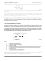
as follows:
0
0

0
K hys = ρ g 
0
0

0
0
0
0
0
0 
0
0
0
0
0 
0 K 33 K 34 K 35
0 

0 K 43 K 44 K 45 K 46
0 K 53 K 54 K 55 K 56 

0
0
0
0
0 
(3.1.1)
where the various terms in the hydrostatic stiffness matrix (K hys ) are:
K 33 = A
K 34 = K 43 = ∫ ydA
A
K 35 = K 53 = − ∫ xdA
A
K 44 = ∫ y dA + z gb ⋅ vol
2
A
K 45 = K 54 = − ∫ xydA
A
K 46 = − x gb ⋅ vol
K 55 = ∫ x 2 dA + z gb ⋅ vol
A
K 56 = − y gb ⋅ vol
The integrals are with respect to the body's cut water-plane and the total area of the cut water-plane is 'A'.
The displaced volume of fluid is given by 'vol'. The following coordinates are also used:
x,y z are the coordinates defined in the body fixed axes.
Contains proprietary and confidential information of ANSYS, Inc. and its subsidiaries and affiliates
Page 12 of 122
AQWA™ LIBRIUM User Manual
x ,y
gb
gb
Theoretical Formulation
and z give the centre of buoyancy with respect to the centre of gravity
gb
Note that K46 and K56 will be zero and the stiffness matrix symmetric if the centre of buoyancy and the
centre of gravity are located on the same vertical line. For a freely floating body in EQUILIBRIUM, this is
automatically the case (however before equilibrium is reached, the matrix will not be symmetric). In
general, if the body is in EQUILIBRIUM under the influence of mooring lines the centre of buoyancy and
the centre of gravity will not be located on the same vertical line. Hence the hydrostatic stiffness matrix
can be asymmetric while the global system stiffness matrix will still be symmetric.
There are instances where the detailed geometry of the bodies is not available or not required. The user
may input directly a buoyancy force and a stiffness matrix which will be assumed constant throughout the
analysis.
3.2 MORISON FORCES
These forces are only determined for tubular members of a structure. The full Morison equation for the
fluid forces acting on a unit length of such a structural member is
dF =
1
ρ D C d (u f − u s ) u f − u s + ρ AC m u f − ρ A(C m − 1) u s
2
( Drag Force )
(3.2.1)
(Wave force) ( Inertia Force )
where
Cd
D
uf
us
Cm
A
ρ
=
=
=
=
=
=
=
drag coefficient
characteristic drag diameter
fluid velocity in the transverse direction of tube
structure velocity in the transverse direction of tube
inertia coefficient
area of cross section
fluid density
Note that all accelerations are zero in AQWA-LIBRIUM.
Full account is taken of fluid velocity variation over the tube length.
The force arising from components of velocity in line with the tube axis is assumed to be zero and forces
acting on the tube end discs are ignored.
Forces and Moments are calculated with respect to the local tube axis system as shown in Figure 3.1, then
transformed to the global axis system.
Contains proprietary and confidential information of ANSYS, Inc. and its subsidiaries and affiliates
Page 13 of 122
AQWA™ LIBRIUM User Manual
Theoretical Formulation
In general a partially submerged tube which is arbitrarily inclined may have a section which is either
completely submerged, partially submerged, or completely out of the water. Each tube element is
classified as above and the forces and moments for each section are summed to obtain the total fluid load.
For static stability calculations only the tube drag force term in the above equation is considered since the
structure and fluid accelerations are not included.
3.3 DIFFRACTION/RADIATION WAVE FORCES
Not applicable to AQWA-LIBRIUM (see AQWA-LINE Manual).
3.4 MEAN WAVE DRIFT FORCES
This section is applicable only if it is considered that the mean wave drift force significantly affects the
equilibrium configuration and the mooring loads.
The mean wave drifting forces and moments are calculated from a set of mean drift coefficients, D(ω), and
a wave energy spectrum, S(ω). The coefficients are specified over a range of frequencies and directions.
The mean wave drift force is given by:
∞
Fd = 2 ∫ 0 S (ω ) D(ω ) dω
(3.4.1)
The coefficients for any specific heading angle are obtained through linear interpolation. If required, these
Contains proprietary and confidential information of ANSYS, Inc. and its subsidiaries and affiliates
Page 14 of 122
AQWA™ LIBRIUM User Manual
Theoretical Formulation
coefficients may be supplied by AQWA-LINE. Only the steady components of the drift forces and
moments are computed in the program (see Section 3.4 of AQWA-LINE User Manual for derivation of the
wave drift coefficients).
3.5 VARIABLE WAVE DRIFT FORCES
Not applicable to AQWA-LIBRIUM (see AQWA-DRIFT Manual).
3.6 INTERACTIVE FLUID LOADING
The hydrodynamic interaction effects on the mean drift forces (near field solution) and added mass matrix
are included.
3.7 STRUCTURAL ARTICULATIONS AND CONSTRAINTS
It is quite common in the analysis of floating systems to have one or more singular degrees of freedom
causing failure in the solution of the equations. For the majority of floating systems, the program checks
and removes these degrees of freedom such that the global stiffness matrix becomes non-singular and the
displacements in the singular coordinates are zero. However, for more complicated systems the user can
constrain directly specific degrees of freedom. This is achieved by assigning the relevant d.o.f. to zero
displacement. The program will automatically uncouple the singular degrees of freedom from the rest.
AQWA also allows structures to be connected by articulated joints. These joints do not permit relative
translation of the two structures but allow relative rotational movement in a number of ways that can
be defined by the user. The reactions at the articulations can be output in global, structure or local
articulation axes.
3.8 WIND AND CURRENT LOADING
The wind and current drag forces are calculated from a set of user prepared empirical environmental load
coefficients covering a range of heading angles. The drag coefficients for any heading are obtained by
linear interpolation. The input load coefficients are defined as
2
( drag force or moment ) / ( wind or current velocity )
According to the above definition, the coefficients are dimensional and the user must conform to a
consistent set of units. (For details see Appendix A of Reference Manual.)
3.9 THRUSTER FORCES
Up to 10 thruster forces may be applied to a body. The magnitude of the thrust vector is constant, and the
Contains proprietary and confidential information of ANSYS, Inc. and its subsidiaries and affiliates
Page 15 of 122
AQWA™ LIBRIUM User Manual
Theoretical Formulation
direction of the vector is fixed to, and moves with, the body. The program will calculate the thruster
moments from the cross product of the latest position vector of the point of application and the thrust
vector.
3.10 MOORING LINES
The effect of mooring lines is to contribute to the external forces and stiffness matrix of a structure. This in
turn will affect the static equilibrium position and its stability in this position.
AQWA-LIBRIUM allows the user to specify the following:
•
•
•
•
•
forces of constant magnitude and direction
constant tension winch lines connecting two bodies (or a body and a fixed point)
linear/non-linear elastic weightless hawsers connecting two bodies (or a body and a fixed point)
composite elastic catenary chains between a body and a sea anchor (or connecting two bodies)
fenders between two bodies (or a body and a fixed point)
N.B.
Current drag on all mooring lines is ignored if without cable dynamics option.
Within the program, the tension vector and stiffness matrix of each mooring line are initially evaluated
with respect to a set of axes local to the vertical plane containing the line. The detailed method by which
the GLOBAL force vector and system stiffness matrix are transformed to the FRA is given in Section
3.10.3.
Force of Constant Magnitude and Direction
A constant "FORCE" line is always assumed to act at the specified point of the body in question. The force
magnitude and direction are assumed fixed and DO NOT CHANGE with movement of the body.
Constant Tension Winch Line
A "WINCH" line maintains a constant tension provided the distance between the ends of the line is
GREATER THAN a user specified 'unstretched length'. The direction of the tension depends on the
movement of the end points.
Weightless Elastic Hawser
The elastic hawser tensions are simply given by the extension over the unstretched length and the
load/extension characteristics. The load/extension characteristics can either be linear (like a spring) or take
the following polynomial form
P(e) = a1e + a 2 e 2 + a3 e 3 + a 4 e 4 + a5 e 5
(3.10.1)
where
P
e
=
=
line tension
extension
For details of the elastic mooring equations, see Section 3.10.1.
Contains proprietary and confidential information of ANSYS, Inc. and its subsidiaries and affiliates
Page 16 of 122
AQWA™ LIBRIUM User Manual
Theoretical Formulation
Elastic Catenary Chain
The submerged weight, length and attachment points of a catenary determine its profile, tension and
stiffness. The standard catenary equations are solved for tension by the Newton-Raphson technique.
Fender
A fender can have a non-linear stiffness (defined by a polynomial as above), friction and damping. It acts
in compression only between a point on one structure and a contact plane on another.
3.10.1 Tension and Stiffness for Mooring Lines with No Mass
The tension in a mooring line whose mass is considered negligible, and thus has no deflection, may be
expressed in terms of a series of coefficients and its extension (e) from an unstretched length. The force
exerted on a structure by the mooring line (P) may therefore be written as
P(e) = a0 + a1e + a 2 e 2 + a3 e 3 + ...
(3.10.2)
Notice that the constant term may be produced when the unstretched length is continually reset to the
actual length (i.e. e = 0). The direction of this force will be given by the vector joining the two attachment
points of the mooring line.
The elastic stiffness in the direction of the force is given by
S (e) = P ′(e) = a1 + 2a 2 e + 3a3 e 2 + ...
(3.10.3)
If this elastic stiffness for a given extension is S, and the tension is P, then the 3x3 stiffness matrix (K),
relating the force to the translational displacements at the attachment point of the structure, may be
expressed as
 l1 
 
S
P
K = N + (I − N) , N = (l1 , l 2 , l3 ) l 2 
L
L
l 
 3
where
(l1 , l 2 , l3 ) =
I
=
L
=
(3.10.4)
unit vector joining the attachment points of the cable
3*3 unit matrix
stretched length of the mooring line
Note that K and the direction vector of the force, P, must be defined in the same axis system. If the axis
system chosen has the X axis coincident with the direction of P, then the stiffness matrix will be diagonal
with S as the value of the leading diagonal term corresponding to the coincident axis and the other two
leading diagonal terms equal to P/L, e.g. for the X axis coincident
Contains proprietary and confidential information of ANSYS, Inc. and its subsidiaries and affiliates
Page 17 of 122
AQWA™ LIBRIUM User Manual
S

K = 0

 0
Theoretical Formulation
0
0 

P
0 
L

0 P 
L
(3.10.5)
If a constant tension device (e.g. a winch) is used at an attachment point then the elastic stiffness S
becomes zero.
Note also that the P/L terms in the equation tend to zero as the mooring line increases in length. This
means that if a mechanism is used at the attachment point to give a constant direction of the force, P, this
has the effect of an infinitely long mooring line, i.e. P/L is zero.
The stiffness matrix, K, for each mooring line is defined at the attachment point on the structure and must
be translated to a common reference point, i.e. the centre of gravity in the AQWA suite. This, as
formulated in Section 3.10.3 as the transformation procedure, is applied to any local stiffness matrix and
force applied at a point on a structure.
3.10.2 Tension and Stiffness for Catenaries
Catenaries in AQWA are considered to be uniform. As the solution of the catenary equations is well
documented (e.g. Berteaux 1976, Barltrop 1998) the summary of the solution used in AQWA is presented.
The equations can be expressed in an axis system whose local X axis is the projection of the vector joining
the attachment points on the sea bed and whose Z axis is vertical. For catenaries which have zero slope at
the contact/attachment point on the sea bed these equations can be written as
2wZ
T
+ 1) 2 −
− AE ,
AE
AE
H
wL
HL
,
X = sinh −1 ( ) +
w
H
AE
V = wL,
H = AE (
T = H 2 +V 2 ,
(3.10.6)
where
L
w
AE
X
Z
H
V
T
=
=
=
=
=
=
=
=
unstretched suspended length;
submerged weight per unit length;
stiffness per length;
horizontal distance between fairlead point on the structure and contact point on seabed;
vertical distance between fairlead point on the structure and contact point on seabed;
horizontal tension;
vertical tension force at the fairlead point;
total tension force at the fairlead point;
A non-linear composite mooring line, in terms of one or more elastic catenaries, can be defined in
AQWA, with intermediate buoys or clump weights between catenaries.
Contains proprietary and confidential information of ANSYS, Inc. and its subsidiaries and affiliates
Page 18 of 122
AQWA™ LIBRIUM User Manual
Theoretical Formulation
A numerical approach is used to calculate the stiffness matrix of composite mooring line.
3.10.3 Translation of the Mooring Line Force and Stiffness Matrix
The formulation of a vector translation may be applied directly to a force and displacement in order to
translate the stiffness matrix, K, from the point of definition to the centre of gravity. It should be noted
however that if the stiffness matrix is defined in a fixed axis system, which does not rotate with the
structure, an additional stiffness term is required. This relates the change of moment created by a constant
force applied at a point when the structure is rotated.
The full 6x6 stiffness matrix (K g ) for each mooring line, relating displacements of the centre of gravity to
the change in forces and moments acting on that structure at the centre of gravity, is therefore given by
[
]
0 
I 
0
K g =  t  [K ] I Ta + 
t ,
Ta 
0 Pm Ta 
(3.10.7)
where
z − y
0

Ta = − z 0
x  ,

 y − x
x, y, z =
 0

Pm = − Pz
 Py

Pz
0
− Px
− Py 

Px 
0 
Coordinates of the attachment point on the structure relative to the centre of gravity.
Px,Py,Pz =
The x,y and z components of the tension in the mooring line at the attachment point on
the structure.
t
The term P m T a is not symmetric. In general, only a structure in static equilibrium will have a symmetric
t
stiffness matrix, where T a is the transpose matrix of T a . However this also means that if the mooring
forces are in equilibrium with all other conservative forces then the total stiffness matrix will be
symmetric.
The force at the centre of gravity ( F g ) in terms of the forces at the attachment point (F a ) is given by
a
[Fg ] = TIt  [Fa ]
 a
(3.10.8)
3.10.4 Stiffness Matrix for a Mooring Line Joining Two Structures
When two structures are attached by a mooring line, this results in a fully-coupled stiffness matrix, where
the displacement of one structure results in a force on the other. This stiffness matrix may be obtained
simply by considering that the displacement of the attachment point on one structure is equivalent to a
negative displacement of the attachment point on the other structure. Using the definitions in the previous
Contains proprietary and confidential information of ANSYS, Inc. and its subsidiaries and affiliates
Page 19 of 122
AQWA™ LIBRIUM User Manual
Theoretical Formulation
section, the 12x12 stiffness matrix K is given by
0
 I 
0
Tat 
0 P T t
m a
K g = − I  [K ][I Ta − I − Tb ] + 


0
0
 t

0
0
− Tb 
G
0 
0
0 
0
0 

0 Pn Tbt 
0
(3.10.9)
where
z − y
0

Tb = − z 0
x  ,

 y − x
 0

Pn = − Pz
 Py

Pz
0
− Px
− Py 

Px 
0 
x, y ,z
=
Coordinates of the attachment point on the second structure relative to its centre
of gravity.
Px,Py,Pz
=
X,Y and Z components of the tension in the mooring line at the attachment point
on the second structure.
3.11 WAVE SPECTRA
The method of wave modelling for irregular seas is achieved within the AQWA suite by the specification
of wave spectra. For further details the user is referred to Appendix E of the AQWA Reference Manual.
3.12 EQUILIBRIUM AND STABILITY ANALYSIS
3.12.1 Solution of the Equilibrium Position
The FRA system is used for the equilibrium and stability analysis of the floating system. Where
force/moment vectors and stiffness matrices are initially evaluated at the LSA (see Section 4.3), the
program will transform the vectors/matrices to the FRA prior to the calculation of equilibrium and
stability.
Multi-Degree of Freedom Systems
Consider the simple case of a wall-sided ship with mass, M, and cut waterplane area, A. If Zo is an initial
guess of the vertical position of the centre of gravity, then dz, the displacement required to move the ship
to the equilibrium position, is given by
dz = F / K
(3.12.1)
where
F
K
=
=
(buoyancy when CG is at Z ) - Mg
sea water density * g * A
0
Contains proprietary and confidential information of ANSYS, Inc. and its subsidiaries and affiliates
Page 20 of 122
AQWA™ LIBRIUM User Manual
Theoretical Formulation
The analysis of a multi-body system is essentially the same as that of the simple example above except that
1
2
3
4
5
the system requires NDOF coordinates to describe its position (NDOF = 6 x Number of bodies)
the system is fully coupled through the actions of the moorings
dz is replaced by a NDOF order vector dX containing the three translations and three rotations of
each of the bodies
F is replaced by a NDOF order vector containing the sum of the residual forces/moments in each of
the coordinates
K = { K } is now the GLOBAL STIFFNESS MATRIX of the system in the sense that K measures
the change in the force/moment in the i-th coordinate due to a change in displacement in the j-th
coordinate only.
ij
ij
The Residual Force/Moment Vector
Before equilibrium is reached, a set of unbalanced forces and moments will act on the bodies. The residual
forces and moments include hydrostatic pressures, weights of the structures, mooring tensions, wind drag,
current drag, thruster forces and steady wave drift forces as described in Sections 3.1 and 3.10.
The Stiffness Matrix
AQWA-LIBRIUM computes all the stiffness contributions directly from analytical expressions for the
load/displacement derivatives, or through the use of numerical differentiation.
Steady wind, current and wave drift forces are only functions of the heading angle. Therefore, their
stiffness contributions are found only in changes in the 'yaw' coordinate (ie K 16 ,K 26 ). At present, the
effect of changes in global thruster forces or moments with heading has not been implemented.
The Stiffness Matrix is non-linear in general. To move the bodies towards equilibrium requires a number
of iterative steps. In each step, the values of the K matrix and the force vector F are re-calculated.
Once the Global System Stiffness Matrix has been formed, the program checks and removes any singular
degrees of freedom (see Section 3.7).
Iteration Towards Equilibrium
Let the initial guess of the structure positions and orientations be represented by the vector X(0),
where
X(0)
(x,y,z)
(p,q,r)
t
=
=
=
{ x 1 ,y 1 ,z 1 ,p 1 ,q 1 ,r 1 ,x 2 ,y 2 ...... }
coordinates of the CG with respect to the FRA, and
finite angular rotations which describe the orientation of the bodies.
The superscripts denote the iteration step and the subscripts denote the body number. The displacement
required in step 1 is given by
dX (1) = K −1 ( X (0) ) F ( X (0) )
(3.12.2)
and the new position of the body, X (1) is given by
Contains proprietary and confidential information of ANSYS, Inc. and its subsidiaries and affiliates
Page 21 of 122
AQWA™ LIBRIUM User Manual
Theoretical Formulation
X (1) = dX (1) ) + X (0)
(3.12.3)
The process is repeated until dX is smaller than the user prescribed limit. It is possible to have more than
one equilibrium position. For instance, a capsized ship can still float in equilibrium if buoyancy is
preserved. Therefore it is important to start off the iteration with an approximation close to the required
solution. Also, because of the non-linearities in the system, it is possible to 'overshoot' and miss the
intended equilibrium position. Hence, in practice, dX can be scaled by a user defined under-relaxation
factor to ensure stability in the iteration scheme.
3.12.2 Static Stability Analysis
The program extracts the eigenvalues of the linearised stiffness matrix at equilibrium by the standard
Jacobi successive rotation method. Positive eigenvalues imply stable equilibrium and zero eigenvalues
imply neutral stability. If any of the eigenvalues are negative in sign, it means that the body will not return
to its equilibrium position after a small disturbance in any of the corresponding modes. These eigenvalues
are analogous to the meta-centric height, GM, in transverse stability analysis of ships.
3.12.3 Dynamic Stability Analysis
Given the static equilibrium position of the floating system, X B , the equations of small motions, X, of the
system about its equilibrium position can be written as
MX = FW + FH − FD − FM
(3.12.4)
where
overdot
FW
FH
FD
FM
=
=
=
=
=
time derivatives
wave exciting force
hull drag force
damping force
mooring force
and M, F W , F H , F F and F M are evaluated at the position X E + X
Expanding, and neglecting terms of second order or higher, the linearised equations of motion of the
system can be expressed as
MX + CX + KX = F
(3.12.5)
These equations of motion can be put into the Hamiltonian form
.
M 0   B   C K   B   F 
 0 M   X +  − M 0   X  =  0 

  
   
(3.12.6)
where
Contains proprietary and confidential information of ANSYS, Inc. and its subsidiaries and affiliates
Page 22 of 122
AQWA™ LIBRIUM User Manual
Theoretical Formulation
B = X
 B   B0 
By letting   =  e λ t , λ = f + iω n , the eigenvalues of equation (3.12.6) can be solved by
X  X 0 
M − 1 C M − 1 K   B 
 B  0

  + λ   =  
0   X 
 X  0
 − I
(3.12.7)
Eigenvectors of the system given by equation (3.12.7), will give the modes of motion of the system as
follows:
1.
2.
3.
f <0
STABLE
f > 0 and ω n = 0 UNSTABLE
f > 0 and ω n ≠ 0 FISHTAILING
Also, the period and damping are given by:
Period
=
2π
ωn
Critical damping (%) =
f
−
f
2
+ ω 2n
× 100%
(3.12.8)
For a single degree of freedom system, the percentage of critical damping can be simplified as
C
Critical damping (%) =
× 100%
2 MK
(3.12.9)
3.13 LIMITATIONS OF THEORETICAL APPLICATIONS
At present AQWA-LIBRIUM only provides stability information which is valid for small displacements
about the equilibrium position. The user should be aware of the limitations of extrapolating such data to
large displacements from equilibrium.
However, a stability report, for a single structure with hydrostatic forces only, can be generated (see
AQWA-Reference 4.16B.5). The report, written in *.LIS file, gives a list of positions of the structure
and the corresponding forces at each position.
The program also has no capacity to model internal compartments within a structure, and hence neither
internal compartment free-surfaces, nor damage effects on the hydrostatic stiffness, nor small angle
stability parameters, are included. These facilities will be included in a later version.
Drag effects on mooring cables are ignored if without the cable dynamics option.
Contains proprietary and confidential information of ANSYS, Inc. and its subsidiaries and affiliates
Page 23 of 122
AQWA™ LIBRIUM User Manual
Modelling Techniques
CHAPTER 4 - MODELLING TECHNIQUES
This chapter relates the theory in the previous section to the general form of the input data required for the
AQWA suite. The sections are closely associated with the sections of the input to the program. All
modelling techniques related to the calculations within AQWA-LIBRIUM are presented. This may
produce duplication between manuals where the calculations are performed by other programs in the suite.
Other modelling techniques which are indirectly related are included to preserve subject integrity; these
are indicated accordingly.
Where modelling techniques are only associated with other programs in the AQWA suite, the information
may be found in the appropriate sections of the respective manuals (the section numbers following
correspond to those in the other manuals as a convenient cross reference).
Users formulating data from sources other than programs in the AQWA suite must consult the literature of
the source used to obtain this data.
Contains proprietary and confidential information of ANSYS, Inc. and its subsidiaries and affiliates
Page 24 of 122
AQWA™ LIBRIUM User Manual
Modelling Techniques
4.1 INTRODUCTION
The model of a floating structure requires different modelling depending on the type of problem that the
user wishes to solve. An approximate model may be acceptable in one analysis or even omitted altogether
in another.
In general, there are only two differences in the models required for each program.
The first is in the description of the structure geometry (the mass distribution model is common), which is
achieved by describing one or more tubes and pressure plates. In total the elements describe the whole
structure, and thus the hydrostatic and hydrodynamic model.
The second is in the description of the environment i.e. mooring lines, wind, current, irregular and regular
waves. These parameters are not common to all programs.
AQWA-DRIFT and AQWA-FER do not necessarily require a hydrostatic or hydrodynamic model but only
the hydrostatic stiffness matrix and hydrodynamic loading coefficients, which are the RESULTS of
calculations on these models. Thus when AQWA-LINE has been run, all these parameters may be
transferred automatically from backing files. If AQWA-LINE has not been run previously, the hydrostatic
stiffness matrix and wave loading coefficients are required as input data.
Hydrostatic model
(AQWA-LINE/LIBRIUM/NAUT)
Panels and tubes. No restrictions
Hydrodynamic model
(AQWA-LINE)
-
Diffracting panels and tubes. Restricted in geometry
and proximity to each other and to the boundaries
Hydrodynamic model
(AQWA-NAUT)
-
Panels and tubes. Restricted only
by size (as a function of wavelength)
In practice this means that there is a hydrodynamic model for AQWA-LINE to which other elements are
added for AQWA-LIBRIUM/NAUT. If the user wishes, and when restrictions allow, a more approximate
model may be defined with fewer elements to minimise computer costs.
4.2 MODELLING REQUIREMENTS FOR AQWA-LIBRIUM
AQWA-LIBRIUM requires models of the inertia, hydrostatic and hydrodynamic properties of the bodies,
the moorings and the environmental loads. Some analyses using AQWA-LIBRIUM might not require all
of these models. For example, a static analysis would not require the hydrodynamic model. In general,
AQWA programs do not require modelling of all aspects of the system for two reasons:
1
The calculations associated with a particular model may have been done previously by one of the
AQWA programs, and the results can be transmitted either through backing files or manually as card
image input.
Contains proprietary and confidential information of ANSYS, Inc. and its subsidiaries and affiliates
Page 25 of 122
AQWA™ LIBRIUM User Manual
2
Modelling Techniques
The mechanics of the system are such that a model is not required.
The models used by AQWA-LIBRIUM follow closely the form used by the rest of the AQWA suite. In
most cases, the same model should be applicable to all AQWA programs. However, the user may choose
to adopt different models of the same system. A typical example is the modelling of the hydrostatics of a
wall-sided pontoon. In AQWA-LIBRIUM, the hydrostatic calculation is not affected by mesh size.
Therefore the complete side of a pontoon may be accurately modelled by one flat quadrilateral pressure
plate. In AQWA-LINE, the mesh size is governed by the wave length but only the wetted part of the hull
requires modelling. Hence the user may choose either to use two different meshes for the two programs or
to use a mesh which is acceptable to both. The former will lead to cheaper AQWA-LIBRIUM runs while
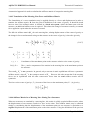
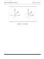
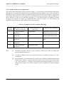
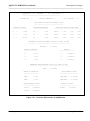
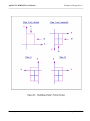
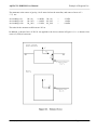
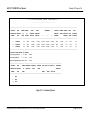
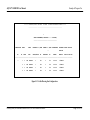
the latter will save the user from the labour of remodelling. (See Figure 4.1 for an illustration of the
differences between an AQWA- LINE and an AQWA-LIBRIUM mesh.)
The general modelling requirements for AQWA-LIBRIUM are:
Analysis
Models
Static
mass, hydrostatics, moorings, current, wind, wave drift, thrusters, constraints.
Dynamic
the same as above plus mass distribution (hence inertia), hydrodynamic properties.
The following subsection describes an exception to the above requirements.
4.2.1 Following an AQWA-LINE Run
An AQWA-LINE run is performed before an AQWA-LIBRIUM run ONLY if it is considered that the
second order mean wave drift forces in an irregular sea will significantly affect the equilibrium
configuration of the system. If this is the case the modelling requirements for AQWA-LIBRIUM will
depend on the type of model used by the AQWA-LINE run. If the AQWA- LINE model includes all nondiffracting elements (e.g. Morison elements, elements above water line), remodelling of the hydrostatic
properties is not required by AQWA-LIBRIUM, unless the user wishes to use a coarser mesh for the
AQWA-LIBRIUM run.
Contains proprietary and confidential information of ANSYS, Inc. and its subsidiaries and affiliates
Page 26 of 122
AQWA™ LIBRIUM User Manual
Modelling Techniques
Figure 4.1a - AQWA-LIBRIUM Mesh
Figure 4.1b - AQWA-LINE Mesh
Contains proprietary and confidential information of ANSYS, Inc. and its subsidiaries and affiliates
Page 27 of 122
AQWA™ LIBRIUM User Manual
Modelling Techniques
4.3 DEFINITION OF STRUCTURE AND POSITION
Full details may be found in the AQWA Reference Manual.
Two sets of axes are used in AQWA-LIBRIUM and these are shown in Figure 4.2. They are the FRA
(Fixed Reference Axes or Global Axes) and the LSA (Local Axes System or Body Fixed Axes). Full
details of the axes systems used in the AQWA suite are given in the AQWA Reference Manual. In
AQWA-LINE, body motions and fluid forces are with respect to the centre of gravity of the particular
body (see Section 3.3 and Figure 4.1).
The AQWA suite employs a single common sign convention with the axes defined as in the AQWA
Reference Manual.
Translations of a structure in the X, Y and Z direction are termed SURGE, SWAY and HEAVE, and are
positive in the positive direction of their respective associated axes. The rotational freedoms are termed
ROLL, PITCH and YAW, and are positive in a clockwise direction when looking along the coordinate
axes from the origin.
The direction of wave or wave spectra propagation is defined relative to the positive X-axis of the FRA,
and is positive in an anticlockwise direction when seen from above. E.g. the heading angle is zero when
the propagation is along the positive X-axis, and 90 degrees when along the positive Y-axis of the FRA.
The position of each body is defined by the coordinates of its centre of gravity with respect to the FRA.
The orientation of the body is defined by three successive rotations about the OX, OY and OZ axes, in
that specific order. Within the program, the orientation is defined by the direction cosines of the BODY
FIXED AXES (LSA) with respect to the FRA.
Contains proprietary and confidential information of ANSYS, Inc. and its subsidiaries and affiliates
Page 28 of 122
AQWA™ LIBRIUM User Manual
Contains proprietary and confidential information of ANSYS, Inc. and its subsidiaries and affiliates
Modelling Techniques
Page 29 of 122
AQWA™ LIBRIUM User Manual
Modelling Techniques
4.4 STRUCTURE GEOMETRY AND MASS DISTRIBUTION
When AQWA-LIBRIUM is used following an AQWA-LINE run, the structure geometry and mass
distribution can be transferred automatically from the backing files produced by AQWA-LINE. This
section therefore describes the modelling of the structure geometry and mass distribution when AQWALIBRIUM is used independently. (See the AQWA-LINE manual when this is not the case.)
4.4.1 Coordinates
Any point on the structure in the modelling process is achieved by referring to the X, Y and Z coordinates
of a point in the FRA which is termed a 'NODE'. The model of structure geometry and mass distribution
consists of a specification of one or more elements (see also Sections 4.1, 4.4.2), each of whose position is
given by one or more nodes. Each node has a node number, which is chosen by the user to be associated
with each coordinate point. Nodes in themselves do not contribute to the model, but may be thought of as a
table of numbers and associated coordinate points to which other parts of the model refer.
Although several coordinates must be defined if several elements are used to define the geometry/mass
distribution, normally a single point mass is used which means that only a single node is defined at the
centre of gravity of the structure.
Note that nodes are also used to define the position of other points not necessarily on the structure, e.g. the
attachment points of each end of a mooring line (see also Section 4.15).
4.4.2 Elements and Element Properties
Each body is modelled by one or more elements which could be a combination of tubes, point masses,
point buoyancies, and quadrilateral and triangular pressure plates. This facility enables simple modelling
of bodies of arbitrary shape. With the exception of plate elements, each element is associated with a set of
material and geometric properties which define the structural masses and inertias of the system. When only
pressure plates are used to simulate the fluid pressure, one or more point mass element with equivalent
mass and inertia is needed to model the mass distribution of the body. (The moment of inertia is required
for the dynamic runs only.)
The program allows the user to take full advantage of symmetry in specific problems. Up to four-fold
symmetry is accommodated.
4.5 MORISON ELEMENTS
Morison elements available within AQWA-LIBRIUM are tubes, slender tubes and discs. Tubes are
defined by specifying end nodes, diameter, wall thickness and end-cut lengths (over which the forces are
ignored). Each tube element may have a different drag and added mass coefficient associated with it. Drag
coefficients can be defined as functions of Reynolds Number.
Full consideration is given to current variation over the tube length, and to partial submersion of members.
Morison drag is evaluated on all submerged or partially submerged tubes, but if the user wishes to
Contains proprietary and confidential information of ANSYS, Inc. and its subsidiaries and affiliates
Page 30 of 122
AQWA™ LIBRIUM User Manual
Modelling Techniques
suppress these calculations the drag coefficient on any or all tubes of a given structure may be set to zero.
Slender tube (STUB) elements differ from TUBE elements in the following respects:
1
STUB elements permit tubes of non-circular cross section to be modelled, by allowing the tube
properties (diameter, drag coefficient, added mass coefficient) to be specified in two directions at
right angles.
2
Longer lengths of tube can be input, as the program automatically subdivides STUB elements into
sections of shorter length for integration purposes.
3
An improved (second order) version of Morisons equation is used to calculate the drag and inertia
forces on STUB elements. This is particularly useful in the study of dropped objects.
4
STUB elements should, however, only be employed if the (mean) diameter is small compared with
the length.
A DISC element (DISC) has no thickness and no mass (users can define a PMAS and attach it to a disc if
necessary), but has drag coefficient and added mass coefficient in its normal direction. Therefore, a DISC
does not have Froude-Krylov and hydrostatic force. A DISC element has only a drag force and an added
mass force.
Reynolds number effects on drag can be important at model scale. Drag coefficients are normally
considered constant (as is often the case at full scale, i.e. large Reynolds numbers). However experimental
evidence shows that Reynolds number is not just a simple function of the velocity and diameter for
cylinders with arbitrary orientation to the direction of the fluid flow. Considerable improvement in
agreement with model tests can be obtained by using a Scale Factor to obtain a local Reynolds Number
and interpolating from classical experimental results,
Local Reynolds Number
where
U
D
=
=
=
=
UD
ν
1
(Scale
factor )3 / 2
Local velocity transverse to the axis of the tube
Tube diameter
Kinematic viscosity of water
from which drag coefficients can be interpolated from the Wieselberg graph of drag coefficient versus
Reynolds number for a smooth cylinder (see AQWA-Reference Appendix G).
Alternatively, a general multiplying factor for drag can be used. It is the interpolated value multiplied by
this factor which is used as the drag coefficient.
Note that for steady state conditions (as in AQWA-LIBRIUM) there are no added mass or slam effects.
Contains proprietary and confidential information of ANSYS, Inc. and its subsidiaries and affiliates
Page 31 of 122
AQWA™ LIBRIUM User Manual
Modelling Techniques
4.6 STATIC ENVIRONMENT
4.6.1 Global Environmental Parameters
The global or static environmental parameters are those which often remain constant or static throughout
an analysis and comprise the following:
Acceleration due to Gravity:
Used to calculate all gravity forces and various dimensionless
variables throughout the program suite
Density of Water:
Used to calculate fluid forces and various dimensionless
variables throughout the program suite
Water Depth:
Used to calculate the clearance from the sea bed (used in the
other programs of the suite to calculate wave properties)
4.7 LINEAR STIFFNESS
This section is only applicable if the user specifies that the stiffness is to be considered linear, i.e. the
stiffness remains linear even for large angle displacement. This is an optional specification (see Appendix
A) and means that a linear hydrostatic stiffness matrix is used in the analysis instead of assembling the
stiffness from the hydrostatic element description.
4.7.1 Hydrostatic Stiffness
There are some cases where a finite element mesh of a body is neither possible (through lack of detailed
geometrical data) nor necessary (e.g. only horizontal planar motion is required, or the movement of the
body is likely to be small). In these cases, the user can model the hydrostatic stiffness of that particular
body via the LSTF option (Linear Stiffness). The LSTF option requires only user input of buoyancy and
hydrostatic stiffness matrix at equilibrium. The program will assume constant buoyancy and stiffness
throughout.
4.7.2 Additional Linear Stiffness
The additional linear stiffness is so called to distinguish between the linear hydrostatic stiffness calculated
by AQWA-LIBRIUM (or AQWA-LINE), and linear stiffness terms from any other mechanism, or for
parametric studies.
Although all terms in the additional linear stiffness can be included in the hydrostatic stiffness matrix, the
user is advised to model the two separately. The most common applications where an additional stiffness
model is useful to have are when
-
modelling facilities for a particular mechanism are not available in the AQWA suite
Contains proprietary and confidential information of ANSYS, Inc. and its subsidiaries and affiliates
Page 32 of 122
AQWA™ LIBRIUM User Manual
Modelling Techniques
-
the hydrostatic stiffness matrix is incomplete
-
the user wishes to investigate the sensitivity of the analysis to changes in the linear stiffness matrix.
N.B. This facility does not replace, but compliments the stiffness due to mooring lines (if present), as
AQWA-LIBRIUM includes the mooring line stiffness in its calculations of the total system stiffness
matrix.
In practice, it is only in unusual applications that the user will find it necessary to consider the modelling
of additional linear stiffness.
4.8 WAVE FREQUENCIES AND DIRECTIONS
The wave frequencies and directions are those at which the wave drift, current and wind coefficients are
defined. Since they are transferred automatically from backing file when AQWA-LIBRIUM is used as a
post- processor, the following notes refer to AQWA-LIBRIUM when used as an independent program.
These coefficients, which are required as input data (further details may be found in the following
sections), are dependent on frequency and/or direction. A range of frequencies and directions is therefore
required as input data, which are those at which the coefficients are defined.
There are only two criteria for the choice of values of frequency and direction which may be summarised
as follows:
1
The extreme values must be chosen to adequately define the coefficients at those frequencies where
wave energy in the spectra chosen (see Section 4.15) is significant, and at all possible directions of
the subsequent response analysis. If geometric symmetry has been specified (see Section 4.3.3) only
those directions for the defined quadrants are required.
2
Sufficient values are required to adequately describe the variation of these coefficients.
Clearly, if either of these criteria is violated, erroneous results will be obtained. Where possible the
program will indicate this accordingly. However, this should not be relied on, as anticipation of the
intentions of the user is not usually possible.
4.9 WAVE LOADING COEFFICIENTS
The mean wave drift force is calculated from a set of drift coefficients, for a range of headings (either
determined from AQWA-LINE or another source), and a wave energy spectrum.
If wave drift coefficients are calculated by AQWA-LINE, they can be transferred automatically from
backing file. (See Section 4.9 of the AQWA-LINE Manual for modelling of the wave drift forces.)
If the coefficients are determined from another source, the coefficients have to be specified for a range of
frequencies and directions as described in the previous Section. The mean drift force at any frequency
within the range is obtained by linear interpolation.
Contains proprietary and confidential information of ANSYS, Inc. and its subsidiaries and affiliates
Page 33 of 122
AQWA™ LIBRIUM User Manual
Modelling Techniques
4.10 WIND AND CURRENT LOADING COEFFICIENTS AND THRUSTERS
The wind and current loading coefficients are required to model the forces and moments on the structure
due to these environmental effects. These forces are proportional to the square of the velocity and produce
terms for steady forces, stiffness and damping.
In the calculation of the equilibrium position and static stability analysis, the effect of the steady forces is
to change the equilibrium position, and thus the stiffness of any non-linear mechanism present (e.g.
catenaries, hydrostatic stiffness). The effect of wind or current stiffness per deg (i.e. rate of change of wind
or current force with yaw) will directly affect both the equilibrium position and the stability. The wind or
current damping has no effect on the static stability calculations.
The wind and current drag loads can be modelled simply as a force, or in more detail, by specifying the
wind and current drag coefficients over a range of wind/current headings, velocity profiles and directions.
The drag coefficients at any heading are obtained by linear interpolation.
4.11 THRUSTER FORCES
Up to ten thruster forces may be specified. The point of application of the force vector is defined by a
NODE. The magnitude of the vector remains constant and the direction of the vector is fixed in relation to
the body fixed axes (LSA).
Note that thruster forces affect the frequency domain solution through the change in equilibrium position
which, in turn, may change the stiffness of any non-linear mechanism present.
4.12 CURRENT AND WIND VELOCITIES AND DIRECTIONS
The wind and current velocities and associated directions can be included along with the spectral
information, as discussed in Section 4.13. In applications where the user is not interested in wave
conditions, the data can be input independently. However this data will be overwritten if current and wind
conditions are specified along with the spectral information. Two types of current velocity can be
specified; the first is a uniform velocity and the second is a profiled current velocity varying with both
direction and depth between the sea-bed and water surface.
4.13 CONSTRAINTS OF STRUCTURE MOTIONS
It is quite common in the analysis of floating systems to have one or more singular degrees of freedom
causing failure in the solution of the equations. For the majority of floating systems, the program checks
and removes these degrees of freedom such that the global stiffness matrix, K, becomes non-singular, and
the displacements in the singular coordinates are zero. However, for more complicated systems the user
can constrain directly specific degrees of freedom. This is achieved by assigning the relevant d.o.f. to a
zero displacement.
Contains proprietary and confidential information of ANSYS, Inc. and its subsidiaries and affiliates
Page 34 of 122
AQWA™ LIBRIUM User Manual
Modelling Techniques
AQWA also allows structures to be connected by articulated joints. These constraints do not permit
relative translation of the two structures but allow relative rotational movement in a number of ways
that can be defined by the user.
There are four different types of articulation available. These are as follows:
0
Ball and Socket
Free to rotate in all freedoms.
1
Universal
Free to rotate in two freedoms transmitting a moment in the third freedom at
right angles to the first two.
2
Hinged
Transmitting a moment in two freedoms and free to rotate in the third
freedom at right angles to the first two.
3
Locked
Transmitting a moment in all three freedoms and not free to rotate at all.
4.14 WAVE SPECTRA, WIND AND CURRENT SPECIFICATION
The user may specify one or more spectra, wind and current speeds, with associated directions, which may
be different for all three. For the majority of applications specification is straightforward and no
knowledge of the way in which the spectra are used in each program is required. The only general rule is
that the value of the spectral ordinate at the beginning and end of the frequency range should be small. If
the values are not small, only part of the spectra has effectively been specified, this may be the intention of
the user however.
4.15 MOORING LINES
4.15.1 Linear/Non-Linear Elastic Hawsers
The line properties are specified by their unstretched lengths, ends nodes on respective bodies and their
load/extension characteristics. For linear hawsers, the line stiffness (load per unit extension) is required.
For non-linear hawsers the program permits up to a fifth order polynomial approximation of the elastic
property of the following form (see Section 3.10.1).
P(e) = a1e + a 2 e 2 + a3 e 3 + a 4 e 4 + a5 e 5
(4.15.1)
where
P
e
=
=
line tension
extension
The use of a higher order polynomial than necessary could lead to erroneous negative stiffness while a
lower order fit could be perfectly adequate (see Figure 4.3). It is always useful to check the polynomial fit
prior to its use as input data. Note, for small extensions, the term a is usually a good approximation to the
linear stiffness.
1
Contains proprietary and confidential information of ANSYS, Inc. and its subsidiaries and affiliates
Page 35 of 122
AQWA™ LIBRIUM User Manual
Modelling Techniques
4.15.2 Constant Tension Winch Line
The winch line is characterised by its constant tension, attachment points and 'unstretched length'. The
attachment points are specified as nodes and determine the direction of the constant tension. The line is
allowed to go slack when the distance between the nodes is less than the 'unstretched length'. If the user
requires constant tension at all times, a zero unstretched length may be input.
4.15.3 ‘Constant Force’ Line
The program allows the user to input a force of constant magnitude and direction. The direction of the
force is specified by a node on the body and a second node chosen such that the force vector is directed
from node 1 to node 2. Once the direction is defined, the program maintains the magnitude and direction
despite movement of the body. This facility can be used to input environmental forces where details of the
forces (e.g. wind coefficients) are not available.
Figure 4.3 - Load/Extension Characteristics
4.15.4 Composite Catenary Line
The composite catenary model admits elastic, catenary lines. Current drag on the line itself is ignored if
without cable dynamics option. The line is specified by the end nodes, length, weight in air per unit length,
and equivalent cross sectional area. The equivalent cross sectional area is numerically equal to the volume
of water displaced by a unit length of the chain.
The user may specify maximum tension in the line and possible highest and lowest vertical relative
positions between the two attachment points.
Contains proprietary and confidential information of ANSYS, Inc. and its subsidiaries and affiliates
Page 36 of 122
AQWA™ LIBRIUM User Manual
Modelling Techniques
The program evaluates the line tension and stiffness. The program allows the line to lift off the sea bed
(i.e. the tangent to the line at the anchor has non-zero slope) up to the point where the line tension exceeds
a user specified/default maximum.
AQWA admits catenary mooring lines between a body and the sloped sea bed (for cable dynamic mooring
line, the seabed is assumed to be horizontal), and a catenary mooring line joining two bodies.
4.15.5 Fender
There are three types of fender; non-directional fixed, directional fixed and floating. The fender is
characterised by its stiffness, size (similar to unstretched length for a mooring line), friction and damping
coefficients. It acts between a node on one body and a contact plane on another body. The stiffness is
defined by a polynomial of up to 5th order (see 4.15.1) although it is compressive instead of tensile. It is
the only way to simulate contact between two bodies in AQWA.
4.16 ITERATION PARAMETERS FOR SOLUTION OF EQUILIBRIUM
4.16.1 Iteration Limits
A well conditioned system coupled with a good initial guess should require a small number of iteration
steps. As a safeguard against modelling errors, the user may limit the number of iteration steps in the first
run. Examination of the output should indicate whether the procedures are converging to a solution or
otherwise. The default is a maximum of 100 steps.
Note that the more accurate the initial estimation of the equilibrium position, the fewer iterations will be
required to find equilibrium. Users should exercise caution in placing the structures in the fluid since the
iteration step is determined using the hydrostatic stiffness (which may be not be defined if the structure is
either submerged or emerged).
4.16.2 Iteration Step Size
Due to the non-linearities in the system, it is quite possible to 'overshoot' and miss the intended equilibrium
configuration. Hence, the program will restrict the movement of each body according to a user specified or
default iteration step size. The step size for each body is characterised by three translations and three
rotations. The program will scale the movement of all the bodies by a constant factor such that none of the
displacements (total of 6 x number of bodies) exceeds its corresponding step size. In other words, equation
(3.12.3) is modified such that
X ( n +1) = C ⋅ dX ( n +1) ) + X ( n)
(4.16.1)
where
C
dS
=
=
Ci
=
Min ( C1 , C 2 , ... ) ,
{ dS 1 , dS 2 ... } is the allowed iteration step size ,
Min(1.0, dS i / dX i( n +1) )
Contains proprietary and confidential information of ANSYS, Inc. and its subsidiaries and affiliates
Page 37 of 122
AQWA™ LIBRIUM User Manual
Modelling Techniques
4.16.3 Convergence Limits
The equilibrium configuration is assumed to be found if the movements of each body, as a result of the
action of residual forces and moments, are smaller than the default or user specified limits. The limits are
specified in terms of the translations and the finite angular rotations of each body.
Contains proprietary and confidential information of ANSYS, Inc. and its subsidiaries and affiliates
Page 38 of 122
AQWA™ LIBRIUM User Manual
Modelling Techniques
4.17 TIME HISTORY INTEGRATION IN IRREGULAR WAVES (AQWA-DRIFT/NAUT)
Not applicable to AQWA-LIBRIUM (see AQWA-DRIFT Manual).
4.18 TIME HISTORY INTEGRATION IN REGULAR WAVES (AQWA-NAUT ONLY)
Not applicable to AQWA-LIBRIUM (see AQWA-NAUT Manual).
4.19 SPECIFICATION OF OUTPUT REQUIREMENTS
See options list (Appendix A).
Contains proprietary and confidential information of ANSYS, Inc. and its subsidiaries and affiliates
Page 39 of 122
AQWA™ LIBRIUM User Manual
Analysis Procedure
CHAPTER 5 - ANALYSIS PROCEDURE
This chapter assumes that the user is familiar with the analysis procedure and how to model the structure
in its environment. It deals with the methodology of analysis associated with running the program, and
links the modelling information in the previous chapter with the stages of analysis necessary to solve a
given type of problem. This involves classification of the types of problem, details of the program runs,
and stages within each program run, together with their associated options.
Contains proprietary and confidential information of ANSYS, Inc. and its subsidiaries and affiliates
Page 40 of 122
AQWA™ LIBRIUM User Manual
Analysis Procedure
5.1 TYPES OF ANALYSIS
Classification of the types of problem (listed below) based on the function of the analysis, is the same
whether the program is used independently, or as a post-processor to AQWA-LINE, and is as follows:
-
Calculation of the static equilibrium positions for a floating system of one or more bodies.
Determination of the hydrostatic loads and the small angle static stability characteristics of the
structures, and the mooring loads within the system when in equilibrium.
-
Calculation of the drift frequency dynamic stability characteristics of the system about a given static
equilibrium position.
All the above are controlled by the job card and may be requested in any combination.
The dynamic stability analysis within both drift frequency range and wave frequency range may be
carried out interactively using the AQWA Graphical Supervisor (AGS).
5.2 RESTART STAGES
All programs in the AQWA suite have the facility of running one or more stages of the analysis separately.
These stages are referred to in the documentation as RESTART STAGES (See AQWA Reference Manual,
Chapter 2).
Use of the restart process implies that information is available on a backing file from a previous program
run and not via the normal card image file. This process is also used to transfer information from one
program to another program in the AQWA suite.
The stages are as follows:
Stage 1
Stage 2
Stage 3
Stage 4
Stage 5
-
Geometric Definition and Static Environment
Input of the Diffraction/Radiation Analysis Parameters
The Diffraction/Radiation Analysis
Input of the Analysis Environment
Motion Analysis
As Stage 3 has no direct calculations in programs other than AQWA-LINE, the programs will 'correct' a
request to finish at Stage 2 to one to finish at Stage 3. This remains transparent and requires no action by
the user.
5.3 STAGES OF ANALYSIS
A typical analysis using AQWA-LIBRIUM requires the following stages:
Contains proprietary and confidential information of ANSYS, Inc. and its subsidiaries and affiliates
Page 41 of 122
AQWA™ LIBRIUM User Manual
Analysis Procedure
1.
Select a consistent set of units.
2.
Assemble geometric and material data for all the structures.
3.
Specify one or more point masses to represent the mass and mass inertia of each of the structures. (In
the case of tubes, structural mass may be input through the geometric properties.)
4.
Calculate the coordinates of the node points for each of the mooring attachments and the elements
used in the modelling of the body.
5.
Specify the water depth and the density of the water.
6.
Specify frequencies and directions and the corresponding drift force coefficients for each structure if
equilibrium is required in a sea state.
7.
For dynamic stability analysis, specify the drift added mass and damping matrices for each structure.
The following preparation is required for AQWA-LIBRIUM, whether used independently, or as a postprocessor to AQWA-LINE:
8.
Prepare thruster forces, and coefficients for wind and current drag, for each structure.
9.
Specify the wave spectra, and the current and wind velocities.
10.
Determine mooring line combinations and properties.
11.
Specify an initial estimate of the equilibrium position of each structure for each spectrum and
mooring line combination.
12.
Code up the above information in a suitable manner acceptable to AQWA-LIBRIUM. (See AQWA
Reference Manual and Chapter 6 of this manual.).
13.
Perform a DATA run (i.e. with the DATA option switched on) which will provide preliminary
checks on the card image data file.
14.
After a successful DATA run, select mode of analysis on the first card of the card image input data
(static/dynamic/both), and re-run with the restart option.
Contains proprietary and confidential information of ANSYS, Inc. and its subsidiaries and affiliates
Page 42 of 122
AQWA™ LIBRIUM User Manual
Data Requirement and Preparation
CHAPTER 6 - DATA REQUIREMENT AND PREPARATION
This chapter describes the form in which data is expected by the program, and is not intended as a detailed
list of the data requirements. Rather it describes the general format for each type of analysis that may be
performed when running AQWA-LIBRIUM. The detailed format may be found in the AQWA Reference
Manual. It also uses the concept of the card image deck which is a section of two or more records, between
which the card image input is divided. It assumes that the user is familiar with this concept, details of
which may also be found in the AQWA Reference Manual.
A summary of the possible data that may be input is listed together with a summary for various forms of
analysis. In the latter case a typical input data summary is given where the more unusual facilities have
been omitted.
Most data requirements listed are optional unless specified otherwise, and if not input the program defaults
are used. These defaults may be found, together with the detailed format description, in the AQWA
Reference Manual.
Contains proprietary and confidential information of ANSYS, Inc. and its subsidiaries and affiliates
Page 43 of 122
AQWA™ LIBRIUM User Manual
Data Requirement and Preparation
6.0 ADMINISTRATION CONTROL - DECK 0 - PRELIMINARY DECK
This deck is always required when performing AQWA program analysis runs. The information input
relates directly to the administration of the job being done and the control of the AQWA program being
used.
Program Control has the following functions:
-
identification of the program to be used within the AQWA suite
the type of program analysis to be performed (if a choice exists)
the analysis stages to be performed (i.e. restart stages)
Administration of the analysis being performed is as follows:
-
user title identification given to the analysis
choice of output required from program run (i.e. program options)
The above information is input to the program through the following cards contained in Deck 0.
JOB Card
- This contains information stating the program to be used, the type of program
analysis to be undertaken, and the user identifier for the run in question.
TITLE Card
- This lets the user prescribe a title for the run.
OPTIONS Card
- Various program options are available within the AQWA suite which are common
to all programs, while others are for use with specific programs. The options
within AQWA-LIBRIUM control the type of output required from the program
and the restart stages of analysis to be performed (see Appendix A).
RESTART Card
- If the restart option is used, then the start and finish stages of the analysis must be
prescribed via the restart card.
For complete details of the above card formats, see the AQWA Reference Manual. For a list of options for
use within AQWA-LIBRIUM, see Appendix A.
One option commonly used is the DATA option and it is worth noting its purpose. The DATA option
performs Stages 1 to 4 of an AQWA-LIBRIUM analysis. This means that all information relating to the
analysis is read, allowing all data checking to be performed. After the user is satisfied with the acceptance
of data, then the equilibrium analysis can be undertaken by restarting the program at Stage 5 to perform the
analysis itself.
6.1 STAGE 1 - DECKS 1 TO 5 - GEOMETRIC DEFINITION AND STATIC ENVIRONMENT
Input for Stage 1 of the analysis is only necessary if the restart stage at which the analysis begins is 1 (see
Contains proprietary and confidential information of ANSYS, Inc. and its subsidiaries and affiliates
Page 44 of 122
AQWA™ LIBRIUM User Manual
Data Requirement and Preparation
Chapter 5 for details). If the restart stage is greater than 1 there should be no data input for Stage 1 of the
analysis.
6.1.1 Description Summary of Physical Parameters Input
The data input in these decks relates to the description of each structure and the environment which
normally remains unchanged throughout the analysis. This includes any point referenced on or
surrounding the structure, the mass inertia, hydrostatic and hydrodynamic model and the (constant) water
depth, i.e.
-
the coordinates of any point on the structure or its surroundings referenced by any other deck
-
element description of the structure mass and geometry using plate, point mass, point buoyancy and
tube elements (see Appendix A of the AQWA Reference Manual for details)
-
a table of material values associated with each element
-
a table of geometric values associated with each element
-
the depth and density of the water, and acceleration due to gravity
The data requirement for each program in the AQWA suite is not the same and may also be dependent on
the type of analysis to be performed. These requirements are listed in detail in the later sections of this
chapter.
6.1.2 Description of General Format
The input format of these decks is designed to provide checking of the data for the average user, and
outputs a suitable message to inform the user if the instructions for data preparation have been
misinterpreted or are unusual. When running the program for the first time it is recommended that the
PRCE option (see Appendix A) is used. This causes the data input in these decks to be output
automatically in order that the user may check the program's interpretation of the data before proceeding to
the next stage of the analysis.
6.1.3 Data Input Summary for Decks 1 to 5
Deck 1
-
The coordinates of points describing the elements
The coordinates of the mooring line attachment points
The coordinates of any points whose position or motions are requested by the
user-specified options
Deck 2
-
Element description of the mass properties
Element description of the hydrostatic model
Element description of the hydrodynamic model
Deck 3
-
A table of material values associated with each element
Contains proprietary and confidential information of ANSYS, Inc. and its subsidiaries and affiliates
Page 45 of 122
AQWA™ LIBRIUM User Manual
Data Requirement and Preparation
Deck 4
-
A table of geometric values associated with each element
Deck 5
-
Static environmental parameters, i.e. the depth and density of the water, and the
acceleration due to gravity
The above information is required before an AQWA-LIBRIUM static/dynamic equilibrium calculation can
be performed. The information contained within Decks 1 to 5 must be input into AQWA-LIBRIUM. The
AQWA Reference Manual gives details of the format for these input data decks.
6.2 STAGE 2 - DECKS 6 TO 8 - THE DIFFRACTION/RADIATION ANALYSIS
PARAMETERS
Input to Stage 2 of the analysis is only necessary if the restart stage at which the analysis begins is 1 or 2
(see Chapter 5). If the restart stage is greater than 2 there is no input necessary for Stage 2 of the analysis.
6.2.1 Description Summary of Physical Parameters Input
The data input in these decks relates to the equation of motion for a diffracting structure or structures,
freely floating in monochromatic waves. The latter are defined for a range of frequencies and directions.
(Note that the structural mass is input in Decks 1 to 5.) For a specified range of frequencies and directions
the equation of motion can be written as
M ( s ) X + M (a ) X + CX + KX = F (d ) + F ( f ) + F ( 2)
(6.2.1)
The parameters in the equation of motion are :
K
-
Linear Stiffness Matrix with associated values of
- The Buoyancy Force at Equilibrium
- The Global Z coordinate of the Centre of Gravity at Equilibrium
and, for each frequency
M(a) C
-
Added Mass Matrix
Radiation Damping Matrix
and, for each frequency and each direction
X
F(d)
F(f)
F(2)
-
Response Motions (or RAOs)
Diffraction Forces
Froude Krylov Forces
Second Order Drift Forces
Of these parameters, only the linear stiffness matrix (with the associated values of the buoyancy force) and
the second order drift forces are applicable to a static analysis using AQWA-LIBRIUM. For dynamic
stability, the added mass and damping matrices for drift frequency motion are also required.
Contains proprietary and confidential information of ANSYS, Inc. and its subsidiaries and affiliates
Page 46 of 122
AQWA™ LIBRIUM User Manual
Data Requirement and Preparation
6.2.2 Description of General Format
The input format and restrictions in these decks are designed to provide maximum cross checking on the
data input when the more advanced facilities are used. This ensures that the program is able to output a
suitable message to inform the user if the instructions for data preparation have been misinterpreted. In any
event, the interpretation of the data input in these decks is output automatically in order that the user may
check the results before proceeding to the next stage of the analysis.
It is important to recognise the different function of the specification of the frequencies and directions
when using AQWA-LINE, which calculates the diffraction/radiation analysis parameters, than when using
other programs to perform an analysis using these parameters. Thus
-
for AQWA-LINE, the range of frequencies and directions specified are those at which the
parameters are to be calculated.
-
for AQWA-LIBRIUM parameters are read from backing file automatically or may be input
manually. In the latter case, the ranges of frequencies and directions specified are those at which the
parameters are to be input within these decks.
Note: Although not directly applicable to AQWA-LIBRIUM, if all the diffraction/radiation parameters are
either read from an AQWA-LINE backing file or input within Deck 7, a natural frequency analysis can be
carried out using the same card image file with the appropriate JOB card. The user is referred to the
AQWA-FER Manual for further details.
6.2.3 Total Data Input Summary for Decks 6 to 8
Deck 6
-
Deck 7
Deck 8
A range of frequencies
A range of directions
Details relating to alterations of the results of a previous run
(all the data in deck 7 are optional if the relevant values are imported from other sources)
Linear hydrostatic stiffness matrix
Additional stiffness matrix (usually not required)
The buoyancy force at equilibrium
Added mass matrix
Additional mass matrix (usually not required)
Radiation damping matrix
Additional linear damping matrix (usually not required)
Diffraction forces
Froude Krylov forces
Response motions (or RAOs - for checking only)
(all the data in deck 8 are optional if the relevant values are imported from other sources)
-
Second Order Drift Forces.
It is unusual for all the data above to be required for any particular analysis, in which case the user simply
omits the data which is not applicable. The following sections show the required data input for the
available modes of analysis.
Contains proprietary and confidential information of ANSYS, Inc. and its subsidiaries and affiliates
Page 47 of 122
AQWA™ LIBRIUM User Manual
Data Requirement and Preparation
6.2.4 Input for AQWA-LIBRIUM using the Results of a Previous AQWA-LINE Run
If there are no changes to the results from a previous AQWA-LINE run, all the data is read automatically
from the backing file and this stage is completely omitted. Thus these decks are not required at all and
must be removed from the card image data deck as the analysis is restarted at the beginning of Stage 4.
Deck 6 to 8
- No Input Required
6.2.5 Input for AQWA-LIBRIUM with Results from Source other than AQWA-LINE
Although the parameters calculated by AQWA-LINE can be transferred automatically to other programs in
the AQWA suite, this is NOT mandatory. This means that if the backing file produced by an AQWALINE run is NOT available (e.g. AQWA-LINE has not been run previously, or the user wishes to input
data from a source other than AQWA-LINE) then data may be input in these decks.
All data appropriate to the analysis (summarised in Section 6.2.3) may then be input in card image format.
The exact input will depend on the type of analysis and the particular structure analysed.
The input data required is:
Case
Deck 6
Deck 7
Deck 8
No drift,
Hydrostatic model
None
None
None
No drift,
No hydrostatic model
None
Linear hydrostatic
stiffness matrix
None
Drift,
Hydrostatic model
Range of frequencies
and directions
None
Second order drift
forces
Drift,
No hydrostatic model
Range of frequencies
and directions
Linear hydrostatic
stiffness matrix
Second order drift
forces
Note that a hydrostatic model may consist of TUBE, TPPL or QPPL elements.
6.2.6 Input for AQWA-LIBRIUM with Results from a Previous AQWA-LINE Run and a
Source other than AQWA-LINE
The new user is advised to ignore this facility
If the user wishes to APPEND to or CHANGE the parameters calculated by a previous AQWA-LINE run
for the current analysis, this can be achieved by using the card image input as described in the previous
section, in addition to reading the results from a previous AQWA-LINE run. As the program does not
expect a database (.HYD) file from AQWA-LINE to exist at Stage 2 of the analysis, the ALDB option
must be used in the options list (see Section 6.0) to indicate that it exists and must be read. Using this
option means that the Stage 2 data is input twice, once from the backing file, and once from the card
image deck.
Alternatively, use FILE/CSTR/CPDB cards in deck 6 to copy the hydrodynamic data from a backing file
Contains proprietary and confidential information of ANSYS, Inc. and its subsidiaries and affiliates
Page 48 of 122
AQWA™ LIBRIUM User Manual
Data Requirement and Preparation
(*.HYD) from a previous run in order to DUPLICATE the database for the structure indicated by the
deck header (see AQWA-Reference 4.6.7).
To APPEND to the parameters calculated in a previous run, additional frequencies which differ from those
existing may be input in Deck 6 together with values of the appropriate frequency dependent parameters in
Decks 7 and 8 at these additional frequencies. Note that as all parameters are defined for a unique range of
directions, these directions must not be redefined.
To change the parameters calculated in a previous run, these parameters are simply input in Decks 7 and 8
and, depending on the type of input (see individual deck sections in the AQWA Reference Manual) the
parameters will be either overwritten with the input values, or become the sum of input values and original
values.
6.3 STAGE 3 - NO CARD IMAGE INPUT - DIFFRACTION/RADIATION ANALYSIS
6.3.1 Stage 3 in AQWA-LIBRIUM
There is no input for Stage 3 in AQWA-LIBRIUM, as this stage corresponds to the Diffraction/Radiation
analysis which has either been performed in AQWA-LINE, or the values from which have been input by
the user from a source other than AQWA-LINE (i.e. when the program is used independently).
6.4 STAGE 4 - DECKS 9 TO 18 - INPUT OF THE ANALYSIS ENVIRONMENT
Input for Stage 4 of the analysis is only necessary if the restart stage at which the analysis begins is a stage
not greater than 4 (see Chapter 5). If the restart stage is greater than 4, there is no input for Stage 4 of the
analysis.
6.4.1 Description of Physical Parameters Input
The data input in these decks relates to the description of the analysis environment, and the structure
coefficients associated with the environment as follows
-
Drift frequency added mass and damping
NB: Drift frequency is a frequency less than the start frequency in the wave spectrum definition.
If the dynamic stability in sea conditions is required from the analysis, it is optional to input the added
mass and damping (which are assumed constant) associated with the drift frequency motion. Otherwise,
the program will obtain these values from the corresponding database in wave frequency range.
-
Wind and current loading coefficients and thruster forces
These coefficients, which are defined at directions specified in Deck 10, or in Deck 6 if a DIRN card is not
present in Deck 10, are associated with the hull drag forces, and are proportional to the square of the wind
Contains proprietary and confidential information of ANSYS, Inc. and its subsidiaries and affiliates
Page 49 of 122
AQWA™ LIBRIUM User Manual
Data Requirement and Preparation
/current velocity. These coefficients also contribute indirectly through the stiffness matrix (i.e. rate of
change of wind or current force with yaw). Linearised current damping on hull is ignored (see Section
4.10) in the dynamic stability calculation. The thruster forces are maintained at both constant magnitude
and direction to the specified structure.
-
Degrees of freedom to be deactivated and constraints
Degrees of freedom can be deactivated by specifying the structure and freedom. This sets the relevant
d.o.f. to zero displacement.
Structures can be connected by articulated joints. These joints do not permit relative translation of the
two structures but allow relative rotational movement in a number of ways that can be defined by the
user.
-
Wave spectra, wind and current
The sea state is defined by a wave spectrum together with its wind and current (see Section 4.14). Wind
spectra and profiled current can be input as well.
-
Mooring lines
The physical characteristics and attachment points of mooring lines, hawsers and tethers may be input if
required (see Section 4.15).
-
Initial estimate of equilibrium positions
The initial estimate of the equilibrium position of each structure can be specified for each mooring line and
spectrum combination required to be analysed.
-
Limits of the iterations to be used in the equilibrium analysis
The maximum, number of iterations, iteration step, and error, considered acceptable, can be specified by
the user. Otherwise the default values will be used.
-
Morison element parameters
These are either the Local Reynolds Number, or the drag scale factor, as applied to the drag coefficients of
Morison elements (already specified in Deck 4) within that structure.
-
Additional output items
Requests for additional listing file output where specific information is required to define its extent
and format. It is supplementary to the output obtained from the general printing requests of the
Options List in the Preliminary Deck, as the requests in this deck are necessarily more detailed.
Contains proprietary and confidential information of ANSYS, Inc. and its subsidiaries and affiliates
Page 50 of 122
AQWA™ LIBRIUM User Manual
Data Requirement and Preparation
6.4.2 AQWA-LIBRIUM Data Input Summary for Decks 9 to 18.
Deck 9
-
Low frequency added mass
Low frequency damping
Deck 10
-
Wind loading coefficients for the superstructure
Current loading coefficients for the hull
Deck 11
-
Wind and current speed and direction when no sea state is specified.
Profiled current data
Deck 12
-
Degrees of freedom of structures which are to be deactivated.
Constraints between structures
Deck 13
-
Wind speed and direction for each spectrum
Current speed and direction for each spectrum
Description of the wave spectra and/or wind spectra
Deck 14
-
Description of each mooring line property
Description of mooring layout for each combination
Deck 15
-
Initial estimates of the equilibrium positions for each spectrum and mooring line
combination to be analysed
Deck 16
-
Iteration and convergence limits
Deck 17
-
Morison element parameters
Deck 18
-
Additional printing options
6.5 STAGE 5 - NO INPUT - EQUILIBRIUM ANALYSIS
This stage performs the search for equilibrium and therefore requires NO INPUT.
Contains proprietary and confidential information of ANSYS, Inc. and its subsidiaries and affiliates
Page 51 of 122
AQWA™ LIBRIUM User Manual
Description of Output
CHAPTER 7 - DESCRIPTION OF OUTPUT
This chapter describes the comprehensive program output provided by AQWA-LIBRIUM.
The various program stages perform different types of analyses and the output for each stage of the
analysis is described in detail in the following sections.
Contains proprietary and confidential information of ANSYS, Inc. and its subsidiaries and affiliates
Page 52 of 122
AQWA™ LIBRIUM User Manual
Description of Output
7.1 STRUCTURAL DESCRIPTION OF BODY CHARACTERISTICS
This information is only output when starting at Stage 1 or the PRDL option is used to print this
information from backing file.
7.1.1 Properties of All Body Elements
The body surface geometry and mass characteristics are input to AQWA-LIBRIUM through input Decks 1
to 4 (see Section 6.1). These data decks define the following parameters (see AQWA Reference Manual):
-
Node numbers and positions
Elements used to model the body
Material properties of the various elements
Geometry group properties of the elements
The information received by AQWA-LIBRIUM to define the body characteristics is output for checking,
and the body's resultant centre of mass and inertia matrix are also output. The nodal coordinates are output
in the FRA and the format is shown in Figure 7.1.
* * * * C O O R D I N A T E
D A T A * * * *
- - - - - - - - - - - - - - -
INPUT
NODE
SEQUENCE
NO.
X
Y
45.000
-45.000
0.000
-45.000
Z
---------------------------------------------1
2
3
1
2
3
4
11
6
13
5
7
…
12
21
22.500
45.000
22.500
0.000
45.000
-45.000
0.000
0.000
0.000
-45.000
-20.000
-45.000
-20.000
-45.000
-45.000
-20.000
-40.000
Figure 7.1 - Nodal Coordinate Output
Contains proprietary and confidential information of ANSYS, Inc. and its subsidiaries and affiliates
Page 53 of 122
AQWA™ LIBRIUM User Manual
Description of Output
Following the nodal coordinates, each body's element topology is output. The body topology describes the
elements used in the model of the body (see Section 4.4.2). Details of each element are also output as seen
in Figure 7.2. The bodies used each have a specific structure number associated with their output, and this
appears in the title of the output.
The element topology output may be enhanced by more detailed information. This is obtained by using the
PPEL program option (i.e. Print Properties of Elements).
* * * * E L E M E N T
T O P O L O G Y
F O R
S T R U C T U R E
1 * * * *
- - - - - - - - - - - - - - - - - - - - - - - - - - - - - - - -
E L E M E N T
NODE
NODE
NODE
NODE
MATERIAL
GEOMETRY
TYPE
NUMBER
NUMBER
NUMBER
NUMBER
NUMBER
NUMBER
1
QPPL
1
2
12
11
0
0
3
QPPL
22
32
31
0
0
NUMBER
-------------------------------------------------------------------------
2
4
QPPL
11
12
QPPL
31
32
21
22
42
21
0
41
0
0
0
…
16
PMAS
999
0
0
0
1
1
Figure 7.2 - Element Topology Output
The body topology output references the material group number which has a mass or density value
associated with it. The material group numbers are output as shown in Figure 7.3.
* * * * M A T E R I A L
P R O P E R T I E S * * * *
- - - - - - - - - - - - - - - - - - -
MATERIAL
GROUP
NUMBER
DENSITY/PARAM 1
PARAM 2
PARAM 3
1
3.3210E+08
0.0000E+00
0.0000E+00
-----------------------------------------------------
Figure 7.3 - Material Property Output
Contains proprietary and confidential information of ANSYS, Inc. and its subsidiaries and affiliates
Page 54 of 122
AQWA™ LIBRIUM User Manual
Description of Output
The topology output also references the Geometry Group numbers used by the user. Each Geometry Group
may have a range of properties associated with it. The number of relevant properties depends on the type
of element under consideration. The Geometry Group numbers and the various parameters within each
group are output as shown in Figure 7.4. Here the Point Mass element has six geometric parameters which
are the prescribed inertia values. The localised element Drag and Added Mass coefficients are also printed.
* * * * G E O M E T R I C
P R O P E R T I E S * * * *
- - - - - - - - - - - - - - - - - - - -
GEOMETRY
INPUT
GROUP
ELEMENT
SEQUENCE
NO.
TYPE
G E O M E T R I C
1
P A R A M E T E R
2
3
N U M B E R
4
------------------------------------------------------------------------------1
1
PMAS
3.6253E+11
0.0000E+00
0.0000E+00
3.4199E+11
… (output line continued below)
5
DRAG
ADDED MASS
COEFFICIENT
COEFFICIENT
C
D
C
A
0.00
0.00
6
-------------------------------------------------0.0000E+00
3.5991E+11
Figure 7.4 - Geometric Property Output
The program, having accepted the user prescribed element distribution, now outputs the resultant Mass and
Inertia characteristics of the first body being modelled. An example of output is shown in Figure 7.5. The
coordinates of the centre of gravity are with respect to the FRA used in defining the body, and the inertia
matrix is about the centre of gravity of the particular body. The types and total number of elements used to
model the body are output. The number of elements output is based on the total coverage of the body's
wetted surface and not the number input when utilising the program symmetry facilities.
Contains proprietary and confidential information of ANSYS, Inc. and its subsidiaries and affiliates
Page 55 of 122
AQWA™ LIBRIUM User Manual
Description of Output
* * * * * MASS
AND
INERTIA
PROPERTIES
OF
STRUCTURE
1 * * * * * * * * *
------------------------------------------------------
ELEMENT TYPE
------------
NUMBER
OF
ELEMENTS
--------
MASS
----
WEIGHT
------
PMAS
1
3.3210E+08
3.2566E+09
QPPL
60
0.0000E+00
0.0000E+00
-----------------------------------------------------------------T O T A L
61
3.3210E+08
3.2566E+09
-----------------------------------------------------------------X
Y
Z
-----------------------------------CENTRE OF GRAVITY
INERTIA MATRIX
0.000
0.000
-10.620
3.625E+11
0.000E+00
0.000E+00
0.000E+00
3.420E+11
0.000E+00
0.000E+00
0.000E+00
3.599E+11
Figure 7.5 - Resultant Mass and Inertia
Contains proprietary and confidential information of ANSYS, Inc. and its subsidiaries and affiliates
Page 56 of 122
AQWA™ LIBRIUM User Manual
Description of Output
7.2 DESCRIPTION OF ENVIRONMENT
This information is output only if the program is starting at Stage 1 or the PRDL option is used to print this
information from backing file.
The environmental parameters within AQWA-LIBRIUM consist only of the water depth and density, and
the gravitational acceleration. The static environment is output as shown in Figure 7.6 and is seen to
contain these values.
* * * * G L O B A L
P A R A M E T E R S * * * *
- - - - - - - - - - - - - - - - -
WATER
DEPTH
DENSITY
OF
ACCELERATION
. . . . . . . . . . . . . . . . =
250.000
WATER
. . . . . . . . . . . . . =
1025.000
DUE
TO GRAVITY . . . . . . . . =
9.806
Figure 7.6 - Static Environment
Contains proprietary and confidential information of ANSYS, Inc. and its subsidiaries and affiliates
Page 57 of 122
AQWA™ LIBRIUM User Manual
Description of Output
Following the static environment data, the wave environment is output and AQWA-LIBRIUM may have
up to 50 wave frequencies/periods and 41 associated wave directions for each body in the analysis. The
output summary of wave frequencies and directions is shown for structure 1 in Figure 7.7.
The output also shows details of other wave related parameters:
-
Wave number, i.e. 2.0* π /(wavelength)
-
Maximum element size (applicable to AQWA-LINE/NAUT)
Depth ratio
The final piece of information given in Figure 7.7 relates to the frequency dependent parameters (i.e. Drift
Forces). If these parameters have not already been input for certain frequencies, then these frequencies are
listed as having undefined parameters.
* * * * W A V E
F R E Q U E N C I E S / P E R I O D S
A N D
D I R E C T I O N S * * * *
- - - - - - - - - - - - - - - - - - - - - - - - - - - - - - - - - - - - - - -
-------------------------------------------------------------------------------------------------STRUCTURE
FREQUENCY FREQUENCY
(RAD/SEC)
(HERTZ)
PERIOD
WAVE
(SECONDS)
NUMBER
WAVE
LENGTH
MAX ELEM
SIZE
DEPTH RATIO
D/L
K*D
PARAMETERS
-------------------------------------------------------------------------------------------------1
1
0.34907
0.05556
18.00
0.01247
503.68
71.96
0.50
3.12
3
0.38080
0.06061
16.50
0.01481
424.38
60.63
0.59
3.70
2
4
5
6
7
0.36960
0.39270
0.41888
0.44880
0.52360
0.05882
0.06250
0.06667
0.07143
0.08333
17.00
16.00
15.00
14.00
12.00
0.01396
0.01574
0.01790
0.02054
0.02796
450.19
399.23
351.06
305.87
224.74
64.31
57.03
50.15
43.70
32.11
0.56
0.63
0.71
0.82
1.11
3.49
3.93
4.47
5.14
6.99
----------------------------------------------------------------------------------------DIRECTIONS
1
2
3
0.00
45.00
90.00
------------------------------------------------------------------------------------------------------------------------------------------------------------------------------------------
Figure 7.7 - Wave Particulars
Contains proprietary and confidential information of ANSYS, Inc. and its subsidiaries and affiliates
Page 58 of 122
AQWA™ LIBRIUM User Manual
Description of Output
7.3 DESCRIPTION OF FLUID LOADING
This information is output only when starting at Stage 1 or 2, or the PRDL option is used to print this
information from backing file from AQWA-LINE.
The output detailing the various types of fluid loading will now be described, and this is done by way of
the different categories of loading.
7.3.1 Hydrostatic Stiffness
The hydrostatic stiffness matrix output by AQWA-LIBRIUM (as shown in Figure 7.8) when printing from
backing file, is in the analysis position used in AQWA-LINE for the diffraction/radiation analysis. If used
independently, the stiffness matrix output is the sum of the hydrostatic stiffness and the additional stiffness
input by the user.
* * * * H Y D R O D Y N A M I C
P A R A M E T E R S
F O R
S T R U C T U R E
1 * * *
- - - - - - - - - - - - - - - - - - - - - - - - - - - - - - - - - - - - - - AT THE FREE-FLOATING EQUILIBRIUM POSITION
----------------------------------------BUOYANCY FORCE . . . . . . . . . . . . =
Z POSITION OF THE CENTRE OF GRAVITY
3.2566E+09
. = -1.0620E+01
STIFFNESS MATRIX
---------------X
Y
Z
RX
RY
RZ
--------------------------------------------------------------------------------X
0.0000E+00
0.0000E+00
0.0000E+00
0.0000E+00
0.0000E+00
0.0000E+00
Y
0.0000E+00
0.0000E+00
0.0000E+00
0.0000E+00
0.0000E+00
0.0000E+00
Z
0.0000E+00
0.0000E+00
8.1414E+07
0.0000E+00
0.0000E+00
0.0000E+00
RX
0.0000E+00
0.0000E+00
0.0000E+00
2.4408E+10
2.7484E+02
6.2820E+02
RY
0.0000E+00
0.0000E+00
0.0000E+00
2.7484E+02
2.4408E+10
9.4230E+02
RZ
0.0000E+00
0.0000E+00
0.0000E+00
0.0000E+00
0.0000E+00
0.0000E+00
Figure 7.8 - Hydrostatic Stiffness Matrix Output
Contains proprietary and confidential information of ANSYS, Inc. and its subsidiaries and affiliates
Page 59 of 122
AQWA™ LIBRIUM User Manual
Description of Output
7.3.2 Wave Drift Forces
The wave drift forces and moments, as functions of wave period and direction, are output as shown in
Figure 7.9. They are given for each body and for the range of user specified frequencies.
The mean wave drift forces are functions of the wave amplitude squared and are given for unit wave
amplitude.
* * * W A V E - D R I F T
L O A D S
F O R
U N I T
W A V E
A M P L I T U D E * * 2
- - - - - - - - - - - - - - - - - - - - - - - - - - - - - - - - - - - - - - - - - - -
* * *
* * * * F O R
S T R U C T U R E
1 * * * *
- - - - - - - - - - - - - - FORCES
FREQUENCY
DIRECTION (DEGREES)
-------------------------------DUE TO (RADIANS/SEC)
0.0
45.0
90.0
------ ------------- -------------------------DRIFT
----SURGE(X)
0.349
5.13E+04 3.58E+04 -2.05E-03
0.370
2.80E+05 1.97E+05 -9.08E-03
0.381
5.88E+05 4.14E+05 -5.33E-02
0.393
6.45E+05 4.54E+05 -1.01E-01
0.419
3.35E+05 2.33E+05 -5.61E-02
0.449
2.43E+05 1.60E+05 -4.76E-02
0.524
3.42E+05 1.50E+05 -6.79E-02
SWAY(Y)
0.349 -1.68E-03 3.58E+04 5.12E+04
0.370
1.40E-02 1.97E+05 2.80E+05
0.381 -4.96E-02 4.14E+05 5.88E+05
0.393
2.43E-02 4.54E+05 6.45E+05
0.419 -1.88E-02 2.33E+05 3.35E+05
0.449
2.25E-02 1.60E+05 2.43E+05
0.524
3.22E-02 1.50E+05 3.42E+05
YAW(RZ)
0.349
1.71E-01 -4.71E+03 -1.62E-02
0.370 -3.77E-01 -3.04E+03 8.05E-02
0.381 -6.28E-01 -2.40E+03 2.06E+00
0.393 -8.06E-01 -1.80E+03 -2.69E+00
0.419 -1.17E+00 -9.31E+02 -1.57E+00
0.449 -4.46E-01 -3.05E+02 -1.66E+00
0.524 -2.85E-01 4.08E+02 -1.70E+00
Figure 7.9 - Wave Drift Forces/Moment (for far field solution)
Contains proprietary and confidential information of ANSYS, Inc. and its subsidiaries and affiliates
Page 60 of 122
AQWA™ LIBRIUM User Manual
Description of Output
7.3.3 Drift Added Mass and Wave Damping
The added mass and wave damping for drift frequencies can therefore be expressed as single added mass
and damping matrices. The added mass and wave damping are expressed in matrix form, and Figure 7.10
shows a typical added mass matrix for body one at the drift frequency (wave damping being output in a
similar fashion).
* * * *
H Y D R O D Y N A M I C
P A R A M E T E R S
F O R
S T R U C T U R E
1
- - - - - - - - - - - - - - - - - - - - - - - - - - - - - - - - - - - - - - -
* * * *
ADDED MASS AT DRIFT FREQUENCY
----------------------------X
Y
Z
RX
RY
RZ
--------------------------------------------------------------------------------X
3.0092E+08
0.0000E+00
0.0000E+00
0.0000E+00
-8.7459E+08
0.0000E+00
Y
0.0000E+00
3.0092E+08
0.0000E+00
8.7459E+08
0.0000E+00
0.0000E+00
Z
0.0000E+00
0.0000E+00
2.3199E+08
0.0000E+00
0.0000E+00
0.0000E+00
RX
0.0000E+00
8.7036E+08
0.0000E+00
8.5698E+10
0.0000E+00
0.0000E+00
RY
-8.7036E+08
0.0000E+00
0.0000E+00
0.0000E+00
8.5698E+10
0.0000E+00
RZ
0.0000E+00
0.0000E+00
0.0000E+00
0.0000E+00
0.0000E+00
1.2209E+11
Figure 7.10 - Added Mass Matrix Output
Contains proprietary and confidential information of ANSYS, Inc. and its subsidiaries and affiliates
Page 61 of 122
AQWA™ LIBRIUM User Manual
Description of Output
7.4 DESCRIPTION OF STRUCTURE LOADING
This section outputs details of the loads on each structure, whether due to wind and current, thrusters, user
applied constraints or mooring lines.
7.4.1 Thruster Forces and Wind and Current Coefficients
The thruster number and associated force vectors (relative to the local system axes (LSA) of the relevant
structure), along with the point of application (expressed in the FRA system), are output as shown in
Figure 7.11.
* * * * W I N D / C U R R E N T
L O A D S
F O R
U N I T
A M P L I T U D E / V E L O C I T Y * * * *
- - - - - - - - - - - - - - - - - - - - - - - - - - - - - - - - - - - - - - - - - - - - - * * * * A N D
T H R U S T E R
F O R C E S
F O R
S T R U C T U R E
1 * * * *
- - - - - - - - - - - - - - - - - - - - - - - - - - - - - - - - - - THRUSTER FORCES
---------------THRUSTER NODE
POSITION OF THRUSTER (FRA)
LOCAL THRUSTER FORCES IN
NUMBER NUMBER
X
Y
Z
SURGE(X)
SWAY(Y)
HEAVE(Z)
------------------------------------------------------------------------------------1
15
45.000
0.000
-20.000 -2.000E+06
0.000E+00
0.000E+00
Figure 7.11 - Thruster Force Output
Contains proprietary and confidential information of ANSYS, Inc. and its subsidiaries and affiliates
Page 62 of 122
AQWA™ LIBRIUM User Manual
Description of Output
In addition, the wind and current, forces and moments, which are functions of direction, are output for
each structure as shown in Figure 7.12.
The wind and current forces which are both a function of the square of velocity are given for unit velocity.
FORCES
FREQUENCY
DIRECTION (DEGREES)
--------------------------------------DUE TO (RADIANS/SEC)
0.0
45.0
90.0
------ ------------- -------------------------WIND
---SURGE(X)
1.32E+03
1.07E+03
0.00E+00
SWAY(Y)
0.00E+00
1.07E+03
1.32E+03
HEAVE(Z)
0.00E+00
0.00E+00
0.00E+00
ROLL(RX)
0.00E+00 -1.94E+04 -2.39E+04
PITCH(RY)
2.39E+04
1.94E+04
0.00E+00
YAW(RZ)
0.00E+00
0.00E+00
0.00E+00
SURGE(X)
2.95E+06
2.40E+06
0.00E+00
SWAY(Y)
0.00E+00
2.40E+06
2.95E+06
HEAVE(Z)
0.00E+00
0.00E+00
0.00E+00
ROLL(RX)
0.00E+00
2.25E+07
2.77E+07
-2.77E+07 -2.25E+07
0.00E+00
CURRENT
-------
PITCH(RY)
YAW(RZ)
0.00E+00
0.00E+00
0.00E+00
Figure 7.12 - Wind and Current Force Coefficients
7.4.2 Structure Constraints
Structure to structure or structure to a fixed point can be connected by articulated joints using DCON
card in Deck12. Four joint types are available in AQWA Suite (see AQWA-Reference 4.12.3). These
joints do not permit relative translation of the two structures but allow relative rotational movement in
a number of ways that can be defined by the user.
One or more specified degrees of freedom of each structure can be deactivated by using DACF card in
DECK12.
The information of joint(s) and the degrees of freedom active for each structure during the analysis is
signified by the character ‘X’ in the constraint table as shown in Figure 7.13.
Contains proprietary and confidential information of ANSYS, Inc. and its subsidiaries and affiliates
Page 63 of 122
AQWA™ LIBRIUM User Manual
* * * *
CONSTRAINT
JOINT
1
0
Description of Output
C O N S T R A I N T S
- - - - - - - - - - -
* * * *
DEFINED ON
AT
IN DIRECTION AND DIRECTION LINKED TO
AT
IN DIRECTION AND DIRECTION
STRUCTURE
NODE
OF NODE
OF NODE
STRUCTURE
NODE
OF NODE
OF NODE
NUMBER
TYPE
NUMBER
NUMBER
NUMBER
NUMBER
NUMBER
NUMBER
NUMBER
NUMBER
----------------------------------------------------------------------------------------------------------------------------0
504
0
0
1
3
0
0
STRUCTURE
ACTIVE FREEDOMS TABLE
NUMBER
X
Y
Z
RX
RY
RZ
---------------------------------------------------------1
X
X
X
X
X
Figure 7.13 - Structure Constraints Table
Contains proprietary and confidential information of ANSYS, Inc. and its subsidiaries and affiliates
Page 64 of 122
AQWA™ LIBRIUM User Manual
Description of Output
7.4.3 Cable/Line Mooring Configurations
The mooring line configurations table (as shown in Figure 7.14), consisting of the individual mooring type
and properties, is output along with the mooring combination and group number. The location of the line is
identified by a pair of structure numbers and node numbers. In the case of linear moorings (i.e. linear lines,
winch loads and constant forces), the properties are included in the general output, either as stiffnesses or
forces. However, in the case of non-linear moorings (i.e. a non-linear hawsers or composite catenary
mooring), the properties are output in an additional table as shown in Figure 7.15. The parameter list
depends on the mooring type, and is defined in the following table:
Table 7.1: Parameters List for Non-linear Moorings
Parameter
number
Note:
Polynomial (curve-fit of
non linear stiffness)
Catenary properties of
each section
Composite line information
1
1st order polynomial
coefficient
Weight/length
Miminum expected vertical
distance between two ends
2
2nd order polynomial
coefficient
Equivalent cross-sectional
area
Maximum expected vertical
distance between two ends
3
3rd order polynomial
coefficient
Stiffness in terms of EA
Sea bed slope at anchor
point
4
4th order polynomial
coefficient
Maximum tension
5
5th order polynomial
coefficient
Unstretched length
(i)
Non-linear moorings can have group properties, whereas the linear moorings have
specific individual properties.
(ii)
A structure number of zero means that the mooring is attached to ground (e.g. a pier,
sea-bed, etc).
(iii) The Equivalent Cross-Sectional Area is equal to the Volumetric Displacement per unit
length of the Catenary. In general, this area is not the same as the Cross-Sectional Area
(e.g. a chain will have a varying Cross-Sectional Area along its length). It is used to
calculate the buoyancy force on the catenary which is assumed to be constant along its
length.
Contains proprietary and confidential information of ANSYS, Inc. and its subsidiaries and affiliates
Page 65 of 122
AQWA™ LIBRIUM User Manual
Description of Output
* * * * C A B L E / M O O R I N G
L I N E
C O N F I G U R A T I O N S * * * *
- - - - - - - - - - - - - - - - - - - - - - - - - - - - - - - - -
+
CABLE ATTACHMENTS( STRUCTURE - 0 - IS GROUND)
--------------------------------------------COMBINATION
CABLE
CABLE
ATTACHED TO
@NODE
LINKED TO
@NODE
UNSTRETCHED
+
NO.
NO.
GROUP
TYPE
STRUCT/ELEM
NO.
STRUCTURE
STIFFNESS
WINCH FRICTION
FORCE OR
NO.
LENGTH
TENSION
WIND-IN PAY-OUT
--------------------------------------------------------------------------------------------------------------1
1
0
LIN
ELASTIC
1
501
0
511
100.000
2
1
NON - LINEAR
1
502
0
512
100.000
3
2
NON - LINEAR
1
503
0
603
400.000
4
2
NON - LINEAR
1
504
0
604
1.472E+06
400.000
Figure 7.14 - Mooring Configuration Table
* * * * C A B L E / M O O R I N G
L I N E
C O N F I G U R A T I O N S * * * *
- - - - - - - - - - - - - - - - - - - - - - - - - - - - - - - - CABLE/HAWSER GROUP CHARACTERISTICS
---------------------------------GROUP
GROUP
2-D L/EXT
PARAMETER
PARAMETER
PARAMETER
PARAMETER
PARAMETER
NUMBER
TYPE
DATABASE
1
2
3
4
5
----------------------------------------------------------------------------------------1
POLYNOMIAL
1.4715E+06
1.0000E+05
1.0000E+04
0.0000E+00
0.0000E+00
2
COMPOSITE
2.4000E+02
2.6000E+02
2.0000E+00
0.0000E+00
0.0000E+00
3
ELASTIC CAT
1.5000E+02
1.0000E-02
6.0000E+08
7.5000E+06
1.0000E+02
4
ELASTIC CAT
1.2000E+02
1.0000E-02
9.0000E+08
7.5000E+06
2.0000E+02
5
ELASTIC CAT
1.7000E+02
1.0000E-02
6.0000E+08
7.5000E+06
1.0000E+02
1
Figure 7.15 - Non-Linear Mooring Properties
Contains proprietary and confidential information of ANSYS, Inc. and its subsidiaries and affiliates
Page 66 of 122
AQWA™ LIBRIUM User Manual
Description of Output
7.5 DESCRIPTION OF ENVIRONMENTAL CONDITIONS
This section outputs the details of the environmental conditions at which equilibrium is required (i.e. wind,
wave and current).
7.5.1 Wind and Current Conditions (no waves)
The wind and current conditions not associated with wave spectra are output as shown in Figure 7.16 (i.e.
the data input in Deck 11). This output consists of uniform wind and current fields with a superimposed
profiled current condition, characterised by a variation of current speed and direction with water depth.
* * * * E N V I R O N M E N T A L
P A R A M E T E R S * * * *
- - - - - - - - - - - - - - - - - - - - - - - -
UNIFORM CURRENT VELOCITY
. . . . . . . . . =
0.800
UNIFORM CURRENT DIRECTION
. . . . . . . . . =
0.000
UNIFORM WIND VELOCITY . .
. . . . . . . . . =
15.000
UNIFORM WIND DIRECTION
. . . . . . . . . =
0.000
DEFAULT DIRECTION OF PROFILED CURRENT . . . . =
0.000
.
CURRENT PROFILES
---------------Z-ORDINATE
W.R.T. SEA LEVEL
CURRENT
VELOCITY
CURRENT
DIRECTION
-250.000
0.000
0.000
-200.000
0.200
0.000
-240.000
0.000
0.100
0.300
0.000
0.000
Figure 7.16 - Wind and Current Conditions
Contains proprietary and confidential information of ANSYS, Inc. and its subsidiaries and affiliates
Page 67 of 122
AQWA™ LIBRIUM User Manual
Description of Output
From the consideration of the influence of sea state on the system equilibrium, the environmental
parameters are specified either as those corresponding to formulated spectra (i.e Pierson-Moskowitz or
Jonswap), or user defined spectra. In the case of formulated spectra, the environmental parameters are
output as shown in Figure 7.17. Included in the parameter list is the spectral type, and the spectral
resolution limits, (i.e. the number of lines and rasters, and the upper and lower frequency cut-offs). The
spectral parameters depend on the spectrum type, and are defined in the following table:
Table 7.2: Spectral Parameters for Formulated Spectra
Parameter Number
Pierson-Moskowitz
Jonswap
1
Significant wave height
Gamma constant
2
Zero cross over period
Alpha constant
Peak spectral frequency
3
The wave direction is also defined for each spectrum along with the associated wind and current speeds
and directions. Note this data will replace the uniform current and wind data output discussed in Section
7.5.1.
* * * * F O R M U L A T E D
W A V E
S P E C T R A * * * *
- - - - - - - - - - - - - - - - - - - - - -
------------------------------------------------------------------------------------SPECTRUM
WAVE
NUMBER NUMBER
NUMBER
TYPE
LINES
1
PIERSON-M
50
5000
0.3000
1.0000
4.0000
11.0000
0.0000
3
JONSWAP
50
5000
0.2985
0.5869
15.0000
0.0022
0.3927
COMBINATION SPECTRUM
OF
OF
RASTERS
LOWER
UPPER
FREQUENCY FREQUENCY
(RAD/SEC) (RAD/SEC)
PARAMETERS
1
2
3
------------------------------------------------------------------------------------2
JONSWAP
50
5000
0.2500
1.5000
4.4290
0.0074
0.4332
…(output line continued below) …
--------------------------------------------SPECTRAL
DIRECTION
(DEGREES)
CURRENT CURRENT
SPEED DIRECTION
(DEGREES)
MEAN
WIND
SPEED
WIND
DIRECTION
(DEGREES)
--------------------------------------------90.0
0.800
0.0
15.0
0.0
0.0
0.800
0.0
15.0
0.0
45.0
0.800
0.0
15.0
0.0
Figure 7.17 - Formulated Spectra and Wind and Current Conditions
Contains proprietary and confidential information of ANSYS, Inc. and its subsidiaries and affiliates
Page 68 of 122
AQWA™ LIBRIUM User Manual
Description of Output
In the case of user defined spectra, the environmental parameters are output as shown in Figure 7.18.
Included in the parameter list is the spectral resolution limits (i.e the number of lines and rasters, and the
upper and lower frequency cut-offs). The spectral parameters are computed from the user defined spectral
ordinates and frequencies (input in Deck 13), and are output as shown in Figure 7.18. These include the
significant wave height, the maximum spectral value, and the associated peak frequency. The wave
spectrum direction is also defined for each spectrum along with the associated wind and current speeds and
directions. This data will replace the uniform current and wind data output discussed in Section 7.5.1.
* * * * U S E R - D E F I N E D
W A V E
S P E C T R A * * * *
- - - - - - - - - - - - - - - - - - - - - - - - ------------------------------------------------------------------------------------SPECTRUM
NUMBER NUMBER
COMBINATION
NUMBER
OF
LINES
LOWER
OF
UPPER
FREQUENCY FREQUENCY
RASTERS
SIGNFCNT
WAVE
(RAD/SEC) (RAD/SEC) HEIGHT
MAX
PEAK
SPECTRAL
SPECTRAL FREQUENCY DIRECTION
VALUE
(RAD/SEC) (DEGREES)
------------------------------------------------------------------------------------1
50
5000
0.3142
1.8850
14.95
31.83
0.6414
0.0
… (output line continued below) …
----------------------------------CURRENT CURRENT
SPEED DIRECTION
WIND
SPEED
(DEGREES)
WIND
DIRECTION
(DEGREES)
----------------------------------0.8
0.0
15.0
0.0
* * * * U S E R - D E F I N E D
W A V E
S P E C T R A * *
- - - - - - - - - - - - - - - - - - - - - - - - FREQUENCY FREQUENCY
NUMBER
ORDINATE
(RAD/SEC)
-------------------------------1
0.3142
2
0.4451
4.0654
3
0.5760
29.0161
4
0.6414
31.8342
5
0.7069
28.5680
6
0.7723
23.2571
7
0.8378
18.0800
8
0.9032
13.7821
9
0.9687
10.4475
10
1.0341
7.9353
11
1.0996
6.0632
12
1.2305
3.6293
13
1.3614
2.2532
14
1.6232
0.9628
15
1.8850
0.0000
0.4618
Figure 7.18 - User Defined Spectra and Wind and Current Conditions
Contains proprietary and confidential information of ANSYS, Inc. and its subsidiaries and affiliates
Page 69 of 122
AQWA™ LIBRIUM User Manual
Description of Output
7.6 ITERATION PARAMETERS
7.6.1 Initial Equilibrium Positions
The initial equilibrium position of the centre of gravity specified by the user for each structure, spectrum
and hawser combination, will be output in the format shown in Figure 7.19. If the user does not specify a
structure's initial position for a given combination, that structure's initial position will correspond to that of
the previous combination. If no position has been specified at all in Deck 15, the structure's centre of
gravity will be output at the original location in the FRA system.
* * * * I N I T I A L
E Q U I L I B R I U M
P O S I T I O N S
O F
T H E * * * *
- - - - - - - - - - - - - - - - - - - - - - - - - - - - - - - - - - - * * * * C E N T R E
O F
G R A V I T Y * * * *
- - - - - - - - - - - - - - - - -
HAWS. COMB
NUMBER
STRUCTURE
NUMBER
SPECTRUM
NUMBER
TRANSLATIONAL POSITION(FRA)
X
Y
Z
ROTATION ABOUT AXES(FRA)
RX
RY
RZ
-----------------------------------------------------------------------------------------------------------1
1
1
0.000
5.000
-11.000
0.000
0.000
0.000
2
2.500
2.500
-11.000
0.000
0.000
0.000
3
5.000
0.000
-11.000
0.000
0.000
0.000
4
10.000
0.000
-11.000
0.000
0.000
0.000
Figure 7.19 -Initial Equilibrium Positions
Contains proprietary and confidential information of ANSYS, Inc. and its subsidiaries and affiliates
Page 70 of 122
AQWA™ LIBRIUM User Manual
Description of Output
7.6.2 Iteration Limits
The iteration limits used in the equilibrium search are output as shown in Figure 7.20. These correspond to
maximum movement in each mode per iteration, and the maximum allowable convergence error for each
degree of freedom of each structure. In addition, the maximum number of iterations is also stated. If these
values are not input in Deck 16, the values in the output will correspond to the program default values (see
AQWA Reference Manual).
* * * * I T E R A T I O N
L I M I T S * * * *
- - - - - - - - - - - - - - - -
MAXIMUM NUMBER OF ITERATIONS . . .
100
STRUCTURE
TRANSLATION
ROTATION(DEGREES)
NUMBER
X
Y
Z
RX
RY
RZ
-------------------------------------------------------------------------------------------1
MAXIMUM MOVEMENT
FOR ONE ITERATION
MAXIMUM ERROR IN FINAL
EQUILIBRIUM POSITION
2.00
2.00
0.50
0.57
0.57
1.43
0.0100
0.0100
0.0100
0.0100
0.0100
0.0100
Figure 7.20 - Iteration Limits
Contains proprietary and confidential information of ANSYS, Inc. and its subsidiaries and affiliates
Page 71 of 122
AQWA™ LIBRIUM User Manual
Description of Output
7.6.3 Iteration Report
An iteration report for each structure is made at the conclusion of each iteration step, specifying each
structure's centre of gravity position and the residual forces and moments at that structure's CG (in an axis
system parallel to the Fixed Reference Axis system). These will be continuously reported, as shown in
Figure 7.21 until either equilibrium is achieved or the maximum number of iterations is exceeded, whereby
an error message will be output. If the user requires further data expansion, a PBIS option in the options
list will generate the component force contributions in the output (e.g. gravity, stiffness, mooring forces
etc). For further details see Appendix A.
*
* * * ITERATION
TOWARDS
THE
EQUILIBRIUM
POSITION * * * *
-------------------------------------------------SPECTRUM NO.
1
MOORING COMBINATION
1
(NO. OF CABLES =
4)
LOCATIONS OF CG
ORIENTATIONS (DEGREES)
STEP STRUCTURE
X
Y
Z
RX
RY
RZ
---------------------------------------------------------------------0
1
0.00
5.00
-11.00
0.00
0.00
0.00
1
1
0.22
3.00
-10.86
0.01
-0.02
0.05
2
1
0.45
1.00
-10.73
0.01
-0.05
0.06
3
1
0.63
0.21
-10.62
0.02
-0.07
-0.02
4
1
0.63
0.21
-10.62
0.01
-0.07
0.01
5
1
0.63
0.21
-10.62
0.01
-0.07
0.01
…(output line continued below) …
RESIDUAL FORCES AND MOMENTS (AXES AT CG PARA. TO FRA)
X
Y
Z
RX
RY
RZ
----------------------------------------------------------1.83E+06 -8.39E+06
3.10E+07
9.41E+07 -9.07E+06
1.18E+06 -5.37E+06
1.98E+07
6.02E+07 -5.83E+06 -2.07E+05
5.24E+05 -2.37E+06
8.73E+06
2.64E+07 -2.55E+06 -3.84E+05
7.08E+02 -4.43E+03 -2.71E+02 -1.11E+05 -2.73E+04
1.26E+02
1.08E+05
-1.08E+02
2.25E+02 -5.30E+02
9.08E+02
3.80E+03 -3.14E+04
-1.08E+02
2.25E+02 -5.30E+02
9.08E+02
3.80E+03 -3.14E+04
Figure 7.21 - Iteration Report
Contains proprietary and confidential information of ANSYS, Inc. and its subsidiaries and affiliates
Page 72 of 122
AQWA™ LIBRIUM User Manual
Description of Output
7.7 STATIC EQUILIBRIUM REPORT
At the conclusion of the equilibrium analysis, a stiffness report is generated for the global system along
with a general static stability assessment. In addition, hydrostatic particulars of the structures and mooring
forces are output to allow the user to assess the contributions from the system components.
7.7.1 Hydrostatic Reports of Freely Floating Structures
Two reports are generated for the structure hydrostatics. The first is common to other programs within the
AQWA-SUITE, and creates hydrostatic fluid loading details output by AQWA-LIBRIUM for each body
in the EQUILIBRIUM position. This hydrostatic output is grouped into the following four categories, and
as shown in Figure 7.22.
1
Hydrostatic Stiffness Matrix at the Centre of Gravity
The coordinates of the centre of gravity are output with respect to the FRA with the body in
the prescribed analysis position. The heave, roll and pitch components of the hydrostatic
stiffness matrix are given with respect to the body's centre of gravity.
2
Hydrostatic Displacement Properties
The actual and equivalent volumetric displacements are given together with the coordinates of
the centre of buoyancy. These coordinates are measured with the body in the equilibrium
position and with respect to the FRA system. The accuracy of the structure equilibrium is
checked by considering the normalised force/moment components output.
3
Cut Water Plane Area Properties
The properties of the body's cut water plane are output, and these include the total area, centre
of area and principal second moments of area. The angle PHI output is the angle between the
body's principal cut waterplane axes and the FRA. (N.B. the X and Y axes of the FRA are on
the free surface.)
4
Small Angle Stability Parameters
These parameters are output in standard naval architectural terms. They include the vertical
distance between the centre of gravity and the centre of buoyancy (measured w.r.t. the centre
of buoyancy). The metacentres are also output together with the metacentric heights. These
allow the restoration per unit degree of rotation to be calculated and output.
Contains proprietary and confidential information of ANSYS, Inc. and its subsidiaries and affiliates
Page 73 of 122
AQWA™ LIBRIUM User Manual
Description of Output
* * * * HYDROSTATIC
PROPERTIES
IN
THE
FREE
FLOATING
POSITION * *
---------------------------------------------------------------- - - - - - - - - - - - - - 1. STIFFNESS MATRIX AT THE CENTRE OF GRAVITY
-------------------------------------------C.O.G
GX=
0.629 GY=
0.205 GZ=
-10.620
HEAVE( Z) =
ROLL(RX) =
PITCH(RY) =
8.141E+07
-2.249E+05
1.004E+06
-2.249E+05
2.441E+10
-1.922E+04
1.004E+06
-1.922E+04
2.441E+10
2. HYDROSTATIC DISPLACEMENT PROPERTIES
-------------------------------------MESH BASED DISPLACEMENT
MASS BASED DISPLACEMENT
. . . . . . . . = 3.24000E+05
. . . . . . . . = 3.24000E+05
POSITION OF THE CENTRE OF BUOYANCY
BX =
BY =
BZ =
AN INCOMPLETE ELEMENT DESCRIPTION OF
THE HULL GIVES OUT OF BALANCE FORCES
AND MOMENTS. IF THE C.O.B. IS NOT
BELOW THE C.O.G. THIS GIVES OUT OF
BALANCE MOMENTS (FORCES ARE DIVIDED
BY THE WEIGHT AND ARE W.R.T. AXES
PARALLEL TO THE FIXED REFERENCE AXES)
FX
FY
FZ
MX
MY
MZ
=
=
=
=
=
=
0.621
0.203
-20.000
0.000
0.000
0.000
-0.002
0.009
0.000
3. CUT WATER PLANE AREA PROPERTIES
---------------------------------CUT WATER PLANE AREA . . . . . . . . . . . = 8.100E+03
CENTRE OF FLOATATION. I.E. CENTROID
POSITION IN THE FIXED REFERENCE AXES
X =
Y =
0.617
0.203
PRINCIPAL SECOND MOMENTS OF AREA
IXX= 5.468E+06
IYY= 5.468E+06
ANGLE THE PRINCIPAL AXES MAKE WITH
THE FIXED REFERENCE AXIS SYSTEM
PHI=
-11.344
4. SMALL ANGLE STABILITY PARAMETERS
----------------------------------DISTANCE BETWEEN C.O.G. AND C.O.B
BG =
9.380
METACENTRIC HEIGHTS WITH RESPECT TO
THE PRINCIPAL AXES OF THE CUT AREA
GMX=
GMY=
7.495
7.495
DISTANCE BETWEEN THE C.O.B. AND THE
METACENTRE (BMX=GMX+BG,BMY=GMY+BG)
BMX=
BMY=
16.875
16.875
RESTORING MOMENT ABOUT THE PRINCIPAL
AXES PER DEGREE ROTATION
MX = 4.260E+08
MY = 4.260E+08
Figure 7.22 - Structure Hydrostatic Properties in the Free Floating Position
Contains proprietary and confidential information of ANSYS, Inc. and its subsidiaries and affiliates
Page 74 of 122
AQWA™ LIBRIUM User Manual
Description of Output
The second hydrostatic report (as shown in Figure 7.23) which is specific to AQWA-LIBRIUM, generates
similar data to the first. However the output coordinate data is referred to the structure centre of gravity (in
an axis system parallel to the FRA system), rather than the FRA system (as in the previous report). This
report is grouped into the following three sections:
1.
The Equilibrium Position
This is the structure CG position and orientation at equilibrium in the Fixed Reference Axis
system. In addition, the structure FRA direction cosines are provided.
2.
Hydrostatic Forces and Moments
The hydrostatic forces and moments acting on the structure are output along with the centre of
buoyancy with respect to the centre of gravity.
3.
Water Plane Properties
The water plane properties are also referred to the structure CG (parallel to the Fixed
Reference Axes) and include the centre of floatation, and the first, second and product
moments of area. This retains the water surface properties used in the calculation of the angle
between the principal and FRA as shown in Figure 7.22.
Contains proprietary and confidential information of ANSYS, Inc. and its subsidiaries and affiliates
Page 75 of 122
AQWA™ LIBRIUM User Manual
Description of Output
* * * * HYDROSTATICS
OF
STRUCTURE
1
AT
EQUILIBRIUM * * * *
---------------------------------------------------SPECTRUM NO.
1
MOORING COMBINATION
1
(NO. OF CABLES =
4)
EQUILIBRIUM POSITION WITH RESPECT TO FRA
---------------------------------------CENTRE OF GRAVITY
--------------------
ORIENTATION(DEGREES)
--------------------
DIRECTION COSINES OF BODY AXES
-------------------------------------
X
=
0.629
RX
=
0.015
X-AXIS
1.000
0.000
0.001
Y
=
0.205
RY
=
-0.067
Y-AXIS
0.000
1.000
0.000
Z
=
-10.620
RZ
=
0.006
Z-AXIS
-0.001
0.000
1.000
HYDROSTATIC FORCES AND MOMENTS (AXES AT CG PARA. TO FRA)
-------------------------------------------------------BUOYANCY =
3.257E+09
CENTRE OF BUOYANCY
--------------------
MOMENTS
--------------------
X
=
-0.009
X
=
-2.834E+07
Y
=
-0.002
Y
=
-6.353E+06
Z
=
-9.380
Z
=
-3.055E+10
WATERPLANE AREA PROPERTIES (AXES AT CG PARA. TO FRA)
----------------------------------------------------AREA =
CENTRE OF FLOATATION
--------------------
8.100E+03
FIRST MOMENT OF AREA
-------------------------
XBAR =
-0.012
AREA*XBAR =
-9.988E+01
YBAR =
-0.003
AREA*YBAR =
-2.237E+01
SECOND MOMENTS OF AREA
---------------------X AXIS =
5.468E+06
Y AXIS =
5.468E+06
PRODUCTS OF AREA
---------------------XY AXIS =
-1.913E+00
Figure 7.23 - Structure Hydrostatics at Equilibrium
Contains proprietary and confidential information of ANSYS, Inc. and its subsidiaries and affiliates
Page 76 of 122
AQWA™ LIBRIUM User Manual
Description of Output
7.7.2 Structure Hydrostatic Stiffness Matrix
The free-floating hydrostatic stiffness matrix is output for each structure as shown in Figure 7.24. This is
the stiffness matrix at the centre of gravity of the structure at equilibrium, but does not include the
stiffness contributions generated by the structure moorings.
* * * * H Y D R O S T A T I C
- - - - - - - - - - -
S T I F F N E S S
- - - - - - - - -
O F
- -
S T R U C T U R E
- - - - - - - - -
1
---
* * * *
X
Y
Z
RX
RY
RZ
-----------------------------------------------------------------------------X
0.000E+00
0.000E+00
0.000E+00
0.000E+00
0.000E+00
0.000E+00
Y
0.000E+00
0.000E+00
0.000E+00
0.000E+00
0.000E+00
0.000E+00
Z
0.000E+00
0.000E+00
8.141E+07
-2.249E+05
1.004E+06
0.000E+00
RX
0.000E+00
0.000E+00
-2.249E+05
2.441E+10
-1.922E+04
2.834E+07
RY
0.000E+00
0.000E+00
1.004E+06
-1.922E+04
2.441E+10
6.353E+06
RZ
0.000E+00
0.000E+00
0.000E+00
0.000E+00
0.000E+00
0.000E+00
Figure 7.24 - Structure Hydrostatic Stiffness Matrix
Contains proprietary and confidential information of ANSYS, Inc. and its subsidiaries and affiliates
Page 77 of 122
AQWA™ LIBRIUM User Manual
Description of Output
7.7.3 Mooring Forces and Stiffness
An output of the mooring forces and stiffness for a component mooring is shown in Figure 7.25. Note that
‘LENGTH-RANGE’ in the figure is the difference between the distance of two mooring line ends and the
unstretched length of mooring line.
These are output for every mooring line and contribute additional stiffness to the global stiffness matrix
(see Figure 7.26).
* * * * M O O R I N G
F O R C E S
A N D
S T I F F N E S S
F O R
S T R U C T U R E
1 * * * *
- - - - - - - - - - - - - - - - - - - - - - - - - - - - - - - - - - - - - - - - - - - SPECTRUM NUMBER
TYPE LENGTH
1
MOORING COMBINATION
1
(NUMBER OF LINES=
4)
NOTE - STRUCTURE 0 IS FIXED
LENGTH- NODE TENSION
RANGE
VERT ANGLE
FORCE X POSN X AT
NODE TENSION
FORCE X POSN X
STIFFNESS
Y
Y STRUC
VERT ANGLE
Y
Y
X
Y
Z
Z
Z
LAID LN
Z
Z
---------------------------------------------------------------------------------------------------------------------------LINE
100.00
0.38
501 5.64E+05
5.64E+05
-1.16E+03
-2.93E+02
45.62
0.21
0.05
0
511 5.64E+05 -5.64E+05
1.16E+03
2.93E+02
146.00
0.00
0.00
1.47E+06 -3.02E+03 -7.63E+02
-3.02E+03 5.62E+03 1.57E+00
-7.63E+02 1.57E+00 5.62E+03
LINE
100.00
0.80
502 1.18E+06 -7.15E+03
1.18E+06
-1.36E+02
0.61
45.20
0.01
0
512 1.18E+06
7.15E+03
-1.18E+06
1.36E+02
0.00
146.00
0.00
1.17E+04 -8.87E+03 1.03E+00
-8.87E+03 1.47E+06 -1.69E+02
1.03E+00 -1.69E+02 1.17E+04
LINE
100.00
1.62
503 2.38E+06 -2.38E+06
-4.64E+03
1.22E+03
-44.38
0.20
-0.05
0
513 2.38E+06
2.38E+06
4.64E+03
-1.22E+03
-146.00
0.00
0.00
1.47E+06 2.82E+03 -7.45E+02
2.82E+03 2.34E+04 -1.45E+00
-7.45E+02 -1.45E+00 2.34E+04
LINE
100.00
1.20
504 1.77E+06 -1.09E+04
-1.77E+06
2.05E+02
0.62
-44.80
-0.01
0
514 1.77E+06
1.09E+04
1.77E+06
-2.05E+02
0.00
-146.00
0.00
1.76E+04 8.93E+03 -1.03E+00
8.93E+03 1.47E+06 -1.68E+02
-1.03E+00 -1.68E+02 1.75E+04
Figure 7.25 - Mooring Force and Stiffness
Contains proprietary and confidential information of ANSYS, Inc. and its subsidiaries and affiliates
Page 78 of 122
AQWA™ LIBRIUM User Manual
Description of Output
7.7.4 Global System Stiffness Matrix
The system stiffnesses are output in the global stiffness matrix, part of which is shown in Figure 7.26. This
comprises the individual structure hydrostatic components and also the contributions from other structures
passed via the moorings. Figure 7.26 shows the stiffness experienced by one structure and other structure
moored to it.
The global stiffness matrix is output only when the PRST option is used (see Appendix A).
* * * * G L O B A L
- - - - - SPECTRUM NO.
S Y S T E M
- - - - - -
1
S T I F F N E S S
- - - - - - - - -
MOORING COMBINATION
1
(NO. OF CABLES =
STRUCTURE
STRUCTURE
1
-------------
M A T R I X * * * *
- - - - - 6)
1
X
Y
Z
RX
RY
RZ
------------------------------------------------------------------------
X
2.530E+06
-6.545E+06
9.232E+03
8.627E+07
3.845E+07
4.360E+06
Y
-6.545E+06
1.777E+07
1.315E+04
-2.350E+08
-9.103E+07
1.369E+07
Z
9.540E+03
1.288E+04
8.645E+07
3.803E+05
-1.521E+07
4.368E+06
RX
8.627E+07
-2.350E+08
3.803E+05
6.540E+09
-1.119E+10
-2.797E+08
RY
3.845E+07
-9.103E+07
-1.521E+07
-1.131E+10
3.287E+11
-1.775E+08
RZ
3.483E+06
1.030E+07
4.729E+06
-2.760E+08
-1.814E+08
1.655E+11
STRUCTURE
STRUCTURE
2
-------------
1
X
Y
Z
RX
RY
RZ
------------------------------------------------------------------------
X
-2.409E+06
6.464E+06
2.638E+04
-8.575E+07
-3.226E+07
7.577E+06
Y
6.464E+06
-1.762E+07
-7.178E+04
2.338E+08
8.658E+07
-1.968E+07
Z
2.638E+04
-7.178E+04
-3.416E+04
1.681E+06
-1.054E+06
-8.379E+05
RX
-8.166E+07
2.227E+08
2.805E+05
-2.941E+09
-1.111E+09
2.133E+08
RY
-3.109E+07
8.344E+07
-1.120E+06
-1.067E+09
-7.008E+08
7.610E+08
RZ
9.396E+07
-2.510E+08
-1.782E+06
3.396E+09
1.949E+09
-1.637E+11
Figure 7.26 - Components of Global Stiffness Matrix
Contains proprietary and confidential information of ANSYS, Inc. and its subsidiaries and affiliates
Page 79 of 122
AQWA™ LIBRIUM User Manual
Description of Output
7.7.5 System Small Displacement Static Stability
An eigenvalue analysis of the global stiffness matrix is carried out from which the system stability can be
assessed. This information is output in the system small displacement static stability report as shown in
Figure 7.27. The system stability is assessed from an eigenvalue analysis of the global stiffness matrix, all
eigenvalues of which must either be defined as stable or neutral for the system to be free from static
instabilities.
* * * * S M A L L
- - - - -
SPECTRUM NO.
D I S P L A C E M E N T
- - - - - - - - - - - 1
S T A T I C
- - - - - -
HAWSER COMBINATION
1
S T A B I L I T Y * * * *
- - - - - - - - -
(NO. OF HAWSERS =
PRINCIPAL COORD.
LOAD PER UNIT DISPLACEMENT
STABILITY
----------------
--------------------------
---------
IN THE PRINCIPAL COORD.
1
2.932E+06
STABLE
2
2.928E+06
STABLE
3
8.147E+07
STABLE
4
2.494E+10
STABLE
5
2.484E+10
STABLE
6
2.933E+08
STABLE
4)
Figure 7.27 - Small Displacement Static Stability Table
Contains proprietary and confidential information of ANSYS, Inc. and its subsidiaries and affiliates
Page 80 of 122
AQWA™ LIBRIUM User Manual
Description of Output
7.8 DYNAMIC STABILITY REPORT
If the user has requested a dynamic stability analysis, the program will output a dynamic stability report
giving the transient stability characteristics of each moored structure for small perturbations from
equilibrium. This information allows the user to assess the dynamic stability of each vessel (e.g. due to a
random seaway, wind gusting, etc), and identify any problem modes of motion which may require a
redesign of the mooring configuration.
Note that the drift frequency added mass and hydrodynamic damping matrices are used in the AQWALIBRIUM dynamic stability analysis. More precise estimation of dynamic stability can be carried out
interactively using the AGS, in which the added mass and hydrodynamic damping matrices near each
natural frequency of the system are used.
7.8.1 Stability Characteristics of Moored Vessel
The dynamic stability characteristics are output as shown in Figure 7.26. Eigenvalues are determined for
each mode of motion, from the real and imaginary parts of which the critical damping, fishtailing period
and stability of that mode of motion can be assessed. The stability regions are defined as follows:
1
STABLE
The structure returns to the equilibrium position by an exponentially
decreasing oscillation at the specified fishtailing period (excessively large
fishtailing periods indicate a non-oscillatory exponential decay).
2
UNSTABLE
There is a steady exponential drift away from the equilibrium position.
3
FISHTAILING
There is an exponentially increasing oscillation about the equilibrium
position at the fishtailing frequency.
* * * * N A T U R A L
F R E Q U E N C I E S
A N D
M O D E S
O F
M O T I O N * * * *
- - - - - - - - - - - - - - - - - - - - - - - - - - - - - - - - - - - - - - SPECTRUM NUMBER
3
FREQUENCY = 0.0524 RADIANS/SEC
PERIOD = 120.00 SECONDS
---------------------------------------------------------------------------------------------------------------------------MODE 1
MODE 2
MODE 3
MODE 4
MODE 5
MODE 6
---------------------------------------------------------------------------------------------------------------------------FREQUENCY(RADIANS/SEC)
0.0336
0.0486
0.0683
0.2369
0.2420
0.3801
PERIOD
(SECONDS)
186.7461
129.3943
91.9647
26.5247
25.9680
16.5292
DAMPING(PER CENT CRIT)
0.0061
1.3099
0.8796
0.0020
0.0018
0.1089
STABILITY
STABLE
STABLE
STABLE
STABLE
STABLE
STABLE
SURGE
SWAY
ROLL
PITCH
HEAVE
TYPE OF MOTION
YAW
---------------------------------------------------------------------------------------------------------------------------STRUCTURE
NUMBER
FREEDOM
AMP
PHASE
AMP
PHASE
AMP
PHASE
AMP
PHASE
AMP
PHASE
AMP
PHASE
---------------------------------------------------------------------------------------------------------------------------1
SURGE(X)
0.000
0.00
9.991
0.00
0.000
0.00
0.000
0.00
0.327
0.00
0.002 179.00
SWAY(Y)
0.647
0.00
0.000
0.00
9.944
0.00
0.433
0.00
0.000
0.00
0.000
0.00
HEAVE(Z)
0.000
0.00
0.001
0.00
0.000
0.00
0.000
0.00
0.011 180.00
10.000
0.00
ROLL (RX)
0.080
0.00
0.000
0.00
0.895
0.00
9.991 180.00
0.000
0.00
0.000
0.00
PITCH(RY)
0.000
0.00
0.425 -180.00
0.000
0.00
0.000
0.00
9.995
0.00
0.050
0.00
YAW (RZ)
9.979 -179.00
0.000
0.00
0.557
-1.00
0.014 180.00
0.000
0.00
0.000
0.00
Figure 7.28 - Moored Vessel Dynamic Stability Characteristics
Contains proprietary and confidential information of ANSYS, Inc. and its subsidiaries and affiliates
Page 81 of 122
AQWA™ LIBRIUM User Manual
Example of Program Use
CHAPTER 8 -EXAMPLE OF PROGRAM USE
In this chapter an example problem using AQWA-LIBRIUM is illustrated. The problem is one in which
AQWA-LINE has been used to perform the analysis Stages 1 to 3. All steps in the subsequent analysis
procedure are clearly shown, from the problem definition, through the data preparation, to the final
analysis run itself. The method used in this chapter can be easily followed by the user, and if so desired,
the user can repeat the whole procedure, using the same data as used here, to obtain the same results. In
this manner the new user can quickly obtain confidence in using the program.
Contains proprietary and confidential information of ANSYS, Inc. and its subsidiaries and affiliates
Page 82 of 122
AQWA™ LIBRIUM User Manual
Example of Program Use
8.1 BOX STRUCTURE
8.1.1 Problem Definition
The first example is a rectangular box structure for which the analysis has been run using AQWA-LINE
for Stages 1 to 3. This is the simplest and most common form of analysis, i.e. an AQWA-LINE run of
Stages 1 to 3 followed by an AQWA-LIBRIUM run. It is assumed that the user is familiar with the box
structure example in AQWA-LINE.
The characteristics of the body are as follows:
Length
Breadth
Depth
Draught
Mass of the body
=
=
=
=
=
90.0 metres
90.0 metres
55.0 metres
40.0 metres
3.321E8 kg
Mass inertia
I xx
=
3.6253E11 kgm
I yy
=
3.4199E11 kgm
I zz
=
3.5991E11 kgm
=
3.321E5 tonnes
2
2
2
The centre of gravity position vector is (0.0,0.0,-10.62) measured with respect to the FRA.
The environmental parameters may be defined as:
Water depth
=
250.0 metres
3
Water density
=
Wave periods
=
Wave directions =
1025.0 kg/metre
12 to 18 seconds
0.0, 45.0 and 90.0 degrees
The box structure is moored by horizontal soft moorings attached to the mid-sides of the box at the water
line as shown in Figure 8.1.
Unstretched length of each mooring line
Stiffness of each mooring line
=
=
100.0 metres
1.471E6 N/m
Contains proprietary and confidential information of ANSYS, Inc. and its subsidiaries and affiliates
Page 83 of 122
AQWA™ LIBRIUM User Manual
Example of Program Use
In addition, a thruster force acts on the vessel side in the X direction, as shown in Figure 8.1.
Structure thruster force, F T = 2.0E6 Newtons
It is required to obtain the equilibrium position of the box in irregular waves for three given sea states.
Note that the analysis is performed using SI units.
Contains proprietary and confidential information of ANSYS, Inc. and its subsidiaries and affiliates
Page 84 of 122
AQWA™ LIBRIUM User Manual
Contains proprietary and confidential information of ANSYS, Inc. and its subsidiaries and affiliates
Example of Program Use
Page 85 of 122
AQWA™ LIBRIUM User Manual
Example of Program Use
8.1.2 Idealisation of Box
The following requires modelling:
-
The mass and inertia properties of the body
-
The surface of the body
Before starting the modelling exercise, it is necessary to decide the definition position of the body with
respect to the FRA. The body is defined such that the bottom of the box is 40 metres below the X-Y plane
of, and parallel to, the FRA. In this example, the DEFINITION position and ANALYSIS position of the
body are the same, as ZLWL value defined in Deck 2 is zero.
8.1.3 The Body Surface
The body has the property of 4-fold symmetry, and this may be utilised when modelling the surface of the
body. We need only describe, therefore, one quarter of the box's surface and this is shown in Figure 8.2.
Type of Plate Element
Since each of the box surfaces is rectangular and planar, we may best utilise QPPL elements.
Sizing of QPPL Elements
The model beneath the free surface is the same as that used in AQWA-LINE and satisfies the AQWALINE modelling criteria (see AQWA-LINE Manual Section 8.1.1). The superstructure is composed of
non-diffracting quadrilateral plates whose only limitation is that the superstructure geometry should be
properly modelled.
Additional nodes were placed on the structure and the fixed locations to represent the mooring attachment
points (see Figure 8.1).
Contains proprietary and confidential information of ANSYS, Inc. and its subsidiaries and affiliates
Page 86 of 122
AQWA™ LIBRIUM User Manual
Contains proprietary and confidential information of ANSYS, Inc. and its subsidiaries and affiliates
Example of Program Use
Page 87 of 122
AQWA™ LIBRIUM User Manual
Example of Program Use
8.1.4 The Body Mass and Inertia
The mass and inertia characteristics are modelled by using a single point mass element (PMAS) placed at
the centre of gravity. This is positioned at X = 0.0, Y = 0.0, Z = -10.62 metres with respect to the FRA. This
PMAS element will have the required mass and inertia properties described by the relevant material and
geometric group properties as follows:
Mass input via material group 1 with associated value of 3.321E8 kg
Inertia input via geometry group 1 with associated values of
2
I xx
=
3.6253E11 kgm
I yy
=
3.4199E11 kgm
I zz
=
3.5991E11 kgm
2
2
and I = I = I = 0.0
xy
yz
zx
8.1.5 AQWA-LINE Analysis
The equilibrium position used to position the structure for each analysis is normally obtained from an
AQWA-LIBRIUM analysis where each drift force has been estimated manually. In simple cases, the
equilibrium positions may be calculated manually as in this case. The equilibrium positions calculated for
the chosen spectra are as shown below:
Spectrum No
1
2
3
Surge (X)
0.0
0.0
0.0
Sway(Y)
0.0
0.0
0.0
Heave(Z)
-10.62
-10.62
-10.62
Roll(RX)
0.0
0.0
0.0
Pitch(RY)
0.0
0.0
0.0
Yaw(RZ)
0.0
0.0
0.0
The model as described in the previous sections was run using AQWA-LINE for Stages 1 to 3 in order to
generate the hydrodynamic data required by the AQWA-LIBRIUM analysis.
8.1.6 Mean Wave Drift Forces
The mean wave drift loads for unit wave amplitude, necessary to determine the equilibrium position of the
structure in the wave spectra, are calculated by AQWA-LINE for each wave frequency and direction.
These mean wave drift forces are proportional to the square of the wave amplitude, and only the horizontal
wave forces and yaw moment are calculated if the far field solution is employed in AQWA-LINE.
Contains proprietary and confidential information of ANSYS, Inc. and its subsidiaries and affiliates
Page 88 of 122
AQWA™ LIBRIUM User Manual
Example of Program Use
8.1.7 Drift Frequency Added Mass and Damping
The dynamic stability analysis requires that the drift frequency added mass and damping are defined. It
may be assumed that at low frequency, the added mass and damping remain constant. The values of added
mass often used are those of the lowest wave frequency input in AQWA-LINE. This is normally a good
approximation. However, for damping, empirical values may be input based on either the experience of the
user, or experimental results. For this example, values of added mass at a frequency 0.349 (period 18 secs)
will be used, whilst hydrodynamic damping is set to be zero by default.
8.1.8 Current and Wind Force Coefficients
Data for the force coefficients for wind and current in this example are based on the projected area
through the centroid in the three directions specified in Deck 6, as well as the drag coefficients at each
heading.
Wind and Current forces per unit velocity acting on the body are given by:
Force = 0.5 * Density * Area * Drag coefficient * cos(relative heading)
In this example, the drag coefficient at heading 0 or 90 degree is 1.6, whilst at 45 degree, it is 1.3.
Thus the forces in the X and Y directions, due to currents at 0, 45 and 90 degree headings, are respectively:
2
2
F x (0), F y (90)
=
0.5 * 1025.0 * (40.0 * 90.0) * 1.6 * cos (0)
=
2.95E6 Ns /m
F y (0), F x (90)
=
0.5 * 1025.0 * (40.0 * 90.0) * 1.6 * sin (0)
=
0.00E0 Ns /m
F x (45), F y (45)
=
0.5 * 1025.0 * (40.0 * 127.0) * 1.3 * cos (45)
=
2.40E6 Ns /m
2
2
2
2
The moments at the centre of gravity (10.62 metres below the waterline, centre of area at Z = -20.0) are:
At a heading of 0
At a heading of 45
At a heading of 90
M x (0)
M y (0)
M x (45)
M y (45)
M x (90)
M y (90)
=
=
=
=
=
=
0.00E0,
-F x (0)*(-10.62+20.0)
F y (45)*(-10.62+20.0)
-F x (45)*(-10.62+20.0)
F y (90)*(-10.62+20.0)
0.00E0
=
=
=
=
-2.77E7
2.25E7
-2.25E7
2.77E7
2
The units for the moment coefficients are Ns /m.
Similarly, the forces on the superstructure due to the wind at 0, 45 and 90 degree headings in the X and Y
directions respectively (for unit velocity) are:
2
2
F x (0), F y (90)
=
0.5 * 1.22 * (15.0 * 90.0) * 1.6 * cos (0)
=
1.32E3 Ns /m
F y (0), F x (90)
=
0.5 * 1.22 * (15.0 * 90.0) * 1.6 * sin (0)
=
0.00E0 Ns /m
F x (45), F y (45)
=
0.5 * 1.22 * (15.0 * 127.0) * 1.3 * cos (45) =
1.07E3 Ns /m
2
2
Contains proprietary and confidential information of ANSYS, Inc. and its subsidiaries and affiliates
2
2
Page 89 of 122
AQWA™ LIBRIUM User Manual
Example of Program Use
The moments at the centre of gravity, 10.62 metres below the waterline, and centre of area at Z =
+7.5, are:
At a heading of 0
At a heading of 45
At a heading of 90
M x (0)
M x (45)
M x (90)
= 0.00E0,
=-1.94E4,
=-2.39E4,
M y (0)
M y (45)
M y (90)
=
=
=
2.39E4
1.94E4
0.00E0
2
The units for the moment coefficients are Ns /m.
In addition, a thruster force of 2E6 N was applied to the box as shown in Figure 8.3, i.e. a thruster force
vector of (-2E6,0,0) newtons.
Contains proprietary and confidential information of ANSYS, Inc. and its subsidiaries and affiliates
Page 90 of 122
AQWA™ LIBRIUM User Manual
Example of Program Use
8.1.9 Sea Spectra, Current and Wind
The following three wave spectra and their associated directions were used in this example:
Spectrum Type
Spectrum 1
Spectrum 2
Spectrum 3
Pierson-Moskowitz
Pierson-Moskowitz
Pierson-Moskowitz
Frequency Range
(radians/sec)
0.30 - 1.00
0.30 - 1.00
0.30 - 1.00
Significant
Wave Height
4.0m
6.0m
8.0m
Zero Crossing
Period
11.0 sec
11.0 sec
11.0 sec
For each spectrum the wind and current speeds and directions used were as follows:
Wind speed
Wind direction
Current speed
Current direction
=
=
=
=
15.0 m/s
0.0 degrees
0.8 m/s
0.0 degrees
8.1.10 Specification of the Mooring Lines
The mooring lines are simple linear elastic hawsers and therefore require one line of input data for each
mooring line. Each line contains the stiffness, unstretched length, and the structure numbers and node
numbers of the two attachment points. For a line joining a structure to a fixed point, the structure number
corresponding to the fixed point should be set to zero. The node numbers and their positions, to which the
mooring lines are attached, must be input in coordinate Deck 1. Each mooring line of 100 metres
unstretched length has a stiffness of 1.471E6 Newtons per metre.
Contains proprietary and confidential information of ANSYS, Inc. and its subsidiaries and affiliates
Page 91 of 122
AQWA™ LIBRIUM User Manual
Example of Program Use
8.1.11 Initial Position for Analysis
The initial position used to position the structure for each equilibrium analysis may be either the value
used in the AQWA-LINE analysis or estimated manually. The initial positions for this analysis were
selected to produce a few iterations to demonstrate the iteration and convergence information given in the
program output. The positions were as shown below:
Spectrum No
1
2
3
Surge (X)
0.0
0.0
0.0
Sway(Y)
0.0
0.0
0.0
Heave(Z)
-11.00
-11.00
-11.00
Roll(RX)
0.0
0.0
0.0
Pitch(RY)
0.0
0.0
0.0
Yaw(RZ)
0.0
0.0
0.0
8.1.12 Iteration Limits for Analysis
The iteration limits used for the equilibrium search in this analysis were
Maximum number of iterations
Displacement tolerances
Rotation tolerances
=
=
=
20
0.01 metres
0.01 degrees
Default values will be used if no data is supplied (see AQWA Reference Manual).
8.1.13 Input Preparation for Data Run (Stage 4)
The AQWA-LINE run (see AQWA-LINE example) has been performed and the following information is
contained on the RESTART backing file produced by AQWA-LINE.
-
input of the node coordinate data
input of the model's element topology with associated material and geometry properties
input of the static environment
the detailed properties of elements used in each body
the final mass and inertia properties of each body
the preliminary diffraction modelling checks
the wave periods and directions
the analysis position of each body
the secondary diffraction modelling checks
hydrostatic calculations for each body
diffraction/radiation analysis giving wave loading coefficients
Contains proprietary and confidential information of ANSYS, Inc. and its subsidiaries and affiliates
Page 92 of 122
AQWA™ LIBRIUM User Manual
Example of Program Use
The decks for the AQWA-LIBRIUM DATA run are shown in Figure 8.4 and the input may be described
as follows:
-
JOB
TITLE
OPTIONS
PRDL
REST
END
RESTART
-
card
card
card
card
provides identifier, program and type of analysis to be used
prescribes a title header for the run
containing the selected options:
print data list from restart file
indicates that a restart run is required
indicates the end of the options list
containing the start and finish stages
Note that the current run, which starts at the beginning of Stage 4 and finishes at the end of Stage 4,
is equivalent to running with the DATA option.
-
Deck 9
This deck has no input and so has a NONE deck header
-
Deck 10
Wind and current force coefficients and thruster forces for the structure
-
Deck 11
This deck has no input and so has a NONE deck header
-
Deck 12
This deck has no input and so has a NONE deck header
-
Deck 13
Description of the wave spectra
Wind speed and direction for the spectra
Current speed and direction for the spectra
-
Deck 14
Description of each mooring line property and combination
Contains proprietary and confidential information of ANSYS, Inc. and its subsidiaries and affiliates
Page 93 of 122
AQWA™ LIBRIUM User Manual
-
Example of Program Use
Deck 15
Initial estimates of the equilibrium positions for the spectra and the mooring line combination
required to be analysed
-
Deck 16
Iteration limits
-
Deck 17
This deck has no input and so has a NONE deck header
-
Deck 18
This deck has no input and so has a NONE deck header
Contains proprietary and confidential information of ANSYS, Inc. and its subsidiaries and affiliates
Page 94 of 122
AQWA™ LIBRIUM User Manual
JOB T001
TITLE
LIBR
STAT
OPTIONS REST END
RESTART
09
10
4
4
NONE
HLD1
Example of Program Use
TEST RUN NUMBER 20 (FLOATING BOX 40M DRAUGHT 48 FACETS)
ALBOX21
10CUFX
1
3
2.9500E6
2.4000E6
0.0000E0
10CURX
1
3
0.0000E0
2.2500E7
2.7700E7
10CUFY
10CURY
1
1
3
0.0000E0
2.4000E6
2.9500E6
3 -2.7700E7 -2.2500E7
0.0000E0
3
1.3200E3
10WIFX
1
3
1.3200E3
10WIRX
1
3
0.0000E4 -1.9400E4 -2.3900E4
10WIFY
10WIRY
END10THRS
1
1
11
NONE
13
SPEC
12
3
0.0000E0
1.0700E3
2.3900E4
1.9400E4
0.8
0.0
15 -2.0000E6
0.0000E0
0.0000E4
NONE
13CURR
13WIND
15.0
13SPDN
90.0
13PSMZ
1.0
4.0
11.0
0.3
1.0
6.0
11.0
0.3
1.0
8.0
11.0
45.0
13SPDN
0.0
13PSMZ
END13PSMZ
MOOR
0.0
0.3
13SPDN
14
1.0700E3
14LINE
1
501
0
511
1.4715E6
100.0
14LINE
1
503
0
513
1.4715E6
100.0
14LINE
END14LINE
15
1
1
STRT
502
504
0
0
512
514
1.4715E6
1.4715E6
100.0
100.0
15POS1
1
1
0.0
0.0
-11.0
END15POS1
3
1
0.0
0.0
-11.0
15POS1
16
2
LMTS
16MXNI
END16MERR
17
18
NONE
1
20
0.0
0.01
0.0
0.01
-11.0
0.01
0.01
0.01
0.01
NONE
Figure 8.4 - Input for Data Run on Box Structure
Contains proprietary and confidential information of ANSYS, Inc. and its subsidiaries and affiliates
Page 95 of 122
AQWA™ LIBRIUM User Manual
Example of Program Use
8.1.14 Information Supplied by Data Run
The DATA run produces the following form of output and is shown in Figures 8.5 to 8.13.
Figure 8.5 AQWA-LIBRIUM Header Page Used for Identification
Figure 8.6 Card Echo (mandatory) for Decks 9 to 20
This is used to check data input
Figure 8.7 Added mass and damping at drift frequency
Figure 8.8 Current and wind information
Figure 8.9 Wind/Current Forces and Thruster Forces
Tabulation of the data input in Deck 10
Figure 8.10 Constraints
This table shows all the freedoms that are active. Articulations are not yet implemented
Figure 8.11 Formulated Spectra
The wave spectrum and current and wind conditions input in Deck 13 is tabulated showing
also the number of spectral lines by default
Figure 8.12 Cable/Mooring Line Configurations
Tabulation of the mooring lines input in Deck 14
Figure 8.13 Initial Equilibrium Positions of the Centre of Gravity
Tabulation of the initial position input in Deck 15
Figure 8.14 Equilibrium Iteration Limits
Tabulation of the iteration limits input in Deck 16
Figure 8.15 Morison Element Parameters
Tabulation of the (default) Morison element parameters
Contains proprietary and confidential information of ANSYS, Inc. and its subsidiaries and affiliates
Page 96 of 122
AQWA™ LIBRIUM User Manual
DATE:28/11/08
JOB T001
LIBR
Example of Program Use
TIME:14:56:37
STAT
TITLE
TEST RUN NUMBER 20 (FLOATING BOX 40M DRAUGHT 48 FACETS)
OPTIONS REST END
RESTART
4
4
AQWA-LIBRIUM VERSION 12.0.00
AAAAAA
AAAAAAAA
AA
AA
AA
AA
AAAAAAAA
AAAAAAAA
AA
AA
AA
AA
AA
AA
AA
AA
LL
LL
LL
LL
LL
LL
LL
LL
LLLLLL
LLLLLL
QQQQQQ
QQQQQQQQ
QQ
QQ
QQ
QQ
QQ
QQ
QQ
QQ
QQ
QQ
QQ QQ QQ
QQQQQQQQ
QQQQQQ
QQ
IIIIII
IIIIII
II
II
II
II
II
II
IIIIII
IIIIII
WW
WW
WW
WW
WW
WW
WW
WW
WW
WW
WW WW WW
WW WW WW
WW WW WW
WWWWWWWWWW
WWWWWWWW
BBBBBBB
BBBBBBBB
BB
BB
BB
BB
BBBBBBB
BBBBBBB
BB
BB
BB
BB
BBBBBBBB
BBBBBBB
AAAAAA
AAAAAAAA
AA
AA
AA
AA
AAAAAAAA
AAAAAAAA
AA
AA
AA
AA
AA
AA
AA
AA
RRRRRRR
RRRRRRRR
RR
RR
RR
RR
RRRRRRRR
RRRRRRR
RRRRR
RR RRR
RR RRR
RR
RRR
IIII
IIII
IIIIII
IIIIII
II
II
II
II
II
II
IIIIII
IIIIII
UU
UU
UU
UU
UU
UU
UU
UU
UU
UU
UU
UU
UU
UU
UU
UU
UUUUUUUU
UUUUUU
MMMMMMMM
MMMMMMMMMM
MM MM MM
MM MM MM
MM MM MM
MM MM MM
MM MM MM
MM MM MM
MM MM MM
MM MM MM
***************************************************************
*
AQWA 12.0 LEGAL NOTICES
*
***************************************************************
*
*
* COPYRIGHT AND TRADEMARK INFORMATION
*
*
*
* Copyright 2008 Ansys, Inc. All rights reserved.
*
* Unauthorized use, distribution or duplication is prohibited.*
*
*
* See the AQWA manuals for the complete Legal Notice.
*
*
*
***************************************************************
JOB TITLE : TEST RUN NUMBER 20 (FLOATING BOX 40M DRAUGHT 48 FACETS)
Figure 8.5 - AQWA-LIBRIUM Header Page used for Identification
Contains proprietary and confidential information of ANSYS, Inc. and its subsidiaries and affiliates
Page 97 of 122
AQWA™ LIBRIUM User Manual
Example of Program Use
DECK 9.1
--------DECK 10.1
--------10CUFX
10CUFY
10CURX
10CURY
10WIFX
10WIFY
10WIRX
10WIRY
END10THRS
1
1
1
1
1
1
1
1
0
3 2.950E+06 2.400E+06 0.000E+00
3 0.000E+00 2.400E+06 2.950E+06
3 0.000E+00 2.250E+07 2.770E+07
3-2.770E+07-2.250E+07 0.000E+00
3 1.320E+03 1.070E+03 0.000E+00
3 0.000E+00 1.070E+03 1.320E+03
3 0.000E+00-1.940E+04-2.390E+04
3 2.390E+04 1.940E+04 0.000E+00
15-2.000E+06 0.000E+00 0.000E+00
0.000E+00
0.000E+00
0.000E+00
0.000E+00
0.000E+00
0.000E+00
0.000E+00
0.000E+00
0.000E+00
0.000E+00
0.000E+00
0.000E+00
0.000E+00
0.000E+00
0.000E+00
0.000E+00
0.000E+00
0.000E+00
0.000E+00
0.000E+00
0.000E+00
0.000E+00
0.000E+00
0.000E+00
0.000E+00
0.000E+00
0.000E+00
0.000
0.000
0.000
0.000
0.000
0.000
0.000
11.000
0.000
11.000
0.000
11.000
0.000
0.000
0.000
0.000
0.000
0.000
0.000
0.000
0.000
0.000
0.000
0.000
DECK 11
------DECK 12
------DECK 13
------13CURR
0
0
0.800
13WIND
0
0
15.000
**** INFORMATION **** UNIFORM WIND
13SPDN
0
0
90.000
13PSMZ
0
0
0.300
13SPDN
0
0
45.000
13PSMZ
0
0
0.300
13SPDN
0
0
0.000
END13PSMZ
0
0
0.300
DECK 14
------14LINE
14LINE
14LINE
END14LINE
1
1
1
1
501
502
503
504
DECK 15
------15POS1
15POS1
END15POS1
1
2
3
0
0
0
0
0
0
0.000
0.000
0.000
0.000
SPEED IS USED
0.000
0.000
1.000
4.000
0.000
0.000
1.000
6.000
0.000
0.000
1.000
8.000
511
512
513
514
1.472E+06
1.472E+06
1.472E+06
1.472E+06
1.000E+02
1.000E+02
1.000E+02
1.000E+02
0.000E+00
0.000E+00
0.000E+00
0.000E+00
0.000E+00
0.000E+00
0.000E+00
0.000E+00
0.000E+00
0.000E+00
0.000E+00
0.000E+00
1
1
1
0.000
0.000
0.000
0.000
0.000
0.000
-11.000
-11.000
-11.000
0.000
0.000
0.000
0.000
0.000
0.000
0.000
0.000
0.000
20
0
0.000
0.010
0.000
0.010
0.000
0.010
0.000
0.010
0.000
0.010
0.000
0.010
DECK 16
------16MXNI
END16MERR
DECK 17
------DECK 18
-------
Figure 8.6 - Card Echo of Decks 9 to 18
Contains proprietary and confidential information of ANSYS, Inc. and its subsidiaries and affiliates
Page 98 of 122
AQWA™ LIBRIUM User Manual
* * * *
H Y D R O D Y N A M I C
Example of Program Use
P A R A M E T E R S
F O R
S T R U C T U R E
1
- - - - - - - - - - - - - - - - - - - - - - - - - - - - - - - - - - - - - - -
* * * *
ADDED MASS AT DRIFT FREQUENCY
-----------------------------
X
Y
Z
RX
RY
RZ
--------------------------------------------------------------------------------X
3.0092E+08
0.0000E+00
0.0000E+00
0.0000E+00
-8.7459E+08
0.0000E+00
Y
0.0000E+00
3.0092E+08
0.0000E+00
8.7459E+08
0.0000E+00
0.0000E+00
Z
0.0000E+00
0.0000E+00
2.3199E+08
0.0000E+00
0.0000E+00
0.0000E+00
RX
0.0000E+00
8.7036E+08
0.0000E+00
8.5698E+10
0.0000E+00
0.0000E+00
RY
-8.7036E+08
0.0000E+00
0.0000E+00
0.0000E+00
8.5698E+10
0.0000E+00
RZ
0.0000E+00
0.0000E+00
0.0000E+00
0.0000E+00
0.0000E+00
1.2209E+11
DAMPING AT DRIFT FREQUENCY
--------------------------
X
Y
Z
RX
RY
RZ
--------------------------------------------------------------------------------X
0.0000E+00
0.0000E+00
0.0000E+00
0.0000E+00
0.0000E+00
0.0000E+00
Y
0.0000E+00
0.0000E+00
0.0000E+00
0.0000E+00
0.0000E+00
0.0000E+00
Z
0.0000E+00
0.0000E+00
0.0000E+00
0.0000E+00
0.0000E+00
0.0000E+00
RX
0.0000E+00
0.0000E+00
0.0000E+00
0.0000E+00
0.0000E+00
0.0000E+00
RY
0.0000E+00
0.0000E+00
0.0000E+00
0.0000E+00
0.0000E+00
0.0000E+00
RZ
0.0000E+00
0.0000E+00
0.0000E+00
0.0000E+00
0.0000E+00
0.0000E+00
Figure 8.7 - Added Mass and Damping at Drift Frequency
Contains proprietary and confidential information of ANSYS, Inc. and its subsidiaries and affiliates
Page 99 of 122
AQWA™ LIBRIUM User Manual
Example of Program Use
* * W I N D / C U R R E N T
L O A D S
F O R
U N I T
A M P L I T U D E / V E L O C I T Y *
- - - - - - - - - - - - - - - - - - - - - - - - - - - - - - - - - - - - - - - - - - - - - * * * * A N D
T H R U S T E R
F O R C E S
F O R
S T R U C T U R E
1 * * * *
- - - - - - - - - - - - - - - - - - - - - - - - - - - - - - - - - - THRUSTER FORCES
---------------THRUSTER NODE
POSITION OF THRUSTER (FRA)
LOCAL THRUSTER FORCES IN
NUMBER NUMBER
X
Y
Z
SURGE(X)
SWAY(Y)
HEAVE(Z)
------------------------------------------------------------------------------------1
15
45.000
0.000
-20.000 -2.000E+06
0.000E+00
0.000E+00
FORCES
FREQUENCY
DIRECTION (DEGREES)
--------------------------------------DUE TO (RADIANS/SEC)
0.0
45.0
90.0
------ ------------- -------------------------WIND
---SURGE(X)
1.32E+03
1.07E+03
0.00E+00
SWAY(Y)
0.00E+00
1.07E+03
1.32E+03
HEAVE(Z)
0.00E+00
0.00E+00
0.00E+00
ROLL(RX)
0.00E+00 -1.94E+04 -2.39E+04
PITCH(RY)
2.39E+04
1.94E+04
0.00E+00
YAW(RZ)
0.00E+00
0.00E+00
0.00E+00
SURGE(X)
2.95E+06
2.40E+06
0.00E+00
SWAY(Y)
0.00E+00
2.40E+06
2.95E+06
HEAVE(Z)
0.00E+00
0.00E+00
0.00E+00
ROLL(RX)
0.00E+00
2.25E+07
2.77E+07
-2.77E+07 -2.25E+07
0.00E+00
CURRENT
-------
PITCH(RY)
YAW(RZ)
0.00E+00
0.00E+00
0.00E+00
Figure 8.8 - Wind/Current Loads and Thruster Forces
Contains proprietary and confidential information of ANSYS, Inc. and its subsidiaries and affiliates
Page 100 of 122
AQWA™ LIBRIUM User Manual
Example of Program Use
* * * * E N V I R O N M E N T A L
P A R A M E T E R S * * * *
- - - - - - - - - - - - - - - - - - - - - - - UNIFORM CURRENT VELOCITY
. . . . . . . . . =
0.800
UNIFORM CURRENT DIRECTION
. . . . . . . . . =
0.000
UNIFORM WIND VELOCITY . .
. . . . . . . . . =
15.000
NO PROFILED CURRENT
-------------------
Figure 8.9 – Current and Wind Information
* * * *
C O N S T R A I N T S
* * * *
- - - - - - - - - - -
STRUCTURE
NUMBER
ACTIVE FREEDOMS TABLE
X
Y
Z
RX
RY
RZ
----------------------------------------------------------
Figure 8.10 - Constraints
Contains proprietary and confidential information of ANSYS, Inc. and its subsidiaries and affiliates
Page 101 of 122
AQWA™ LIBRIUM User Manual
Example of Program Use
* * * * F O R M U L A T E D
W A V E
S P E C T R A * * * *
- - - - - - - - - - - - - - - - - - - - - - -
---------------------------------------------------------------------------------------------------------------------------------SPECTRUM
WAVE
NUMBER NUMBER
NUMBER
TYPE
LINES
COMBINATION SPECTRUM
OF
LOWER
OF
RASTERS
UPPER
FREQUENCY FREQUENCY
(RAD/SEC) (RAD/SEC)
PARAMETERS
1
2
SPECTRAL
3
DIRECTION
(DEGREES)
CURRENT CURRENT
SPEED DIRECTION
(DEGREES)
MEAN
WIND
SPEED
WIND
DIRECTION
(DEGREES)
---------------------------------------------------------------------------------------------------------------------------------1
PIERSON-M
2
50
PIERSON-M
3
50
PIERSON-M
50
5000
5000
5000
0.3000
0.3000
0.3000
1.0000
1.0000
1.0000
4.0000
6.0000
8.0000
11.0000
11.0000
11.0000
0.0000
0.0000
0.0000
90.0
45.0
0.0
0.800
0.800
0.800
0.0
0.0
0.0
15.0
15.0
15.0
0.0
0.0
0.0
---------------------------------------------------------------------------------------------------------------------------------ASSOCIATED WIND SPECTRA (IF DEFINED)
Freq range(rad/sec)
0.0063
6.2832
Period Range(seconds)= 1000.0000
1.0000
Freq range(Hertz)
=
=
0.0010
1.0000
----------------------------------------------------------------------------------------------------SPECTRUM
WIND
NUMBER REFERENCE
NUMBER
TYPE
LINES
COMBINATION SPECTRUM
OF
ELEVATION
FREQUENCY
COEFF
SPECTRUM
COEFF
VELOCITIES AT 10M REF HT
SHEAR
MEAN
STAN.DEV.
TURBULENCE
INTENSITY
----------------------------------------------------------------------------------------------------1
NULL
3
NULL
2
NULL
Figure 8.11 – Formulated Spectra
Contains proprietary and confidential information of ANSYS, Inc. and its subsidiaries and affiliates
Page 102 of 122
AQWA™ LIBRIUM User Manual
Example of Program Use
* * * * C A B L E / M O O R I N G
L I N E
C O N F I G U R A T I O N S * * * *
- - - - - - - - - - - - - - - - - - - - - - - - - - - - - - - - +
CABLE ATTACHMENTS( STRUCTURE - 0 - IS GROUND)
--------------------------------------------COMBINATION
CABLE
CABLE
ATTACHED TO
@NODE
LINKED TO
@NODE
UNSTRETCHED
+
NO.
NO.
GROUP
TYPE
STRUCT/ELEM
NO.
STRUCTURE
STIFFNESS
WINCH FRICTION
FORCE OR
NO.
LENGTH
TENSION
WIND-IN PAY-OUT
--------------------------------------------------------------------------------------------------------------1
1
0
LIN
ELASTIC
1
501
0
511
100.000
1.472E+06
2
0
LIN
ELASTIC
1
502
0
512
100.000
1.472E+06
3
0
LIN
ELASTIC
1
503
0
513
100.000
1.472E+06
4
0
LIN
ELASTIC
1
504
0
514
100.000
1.472E+06
Figure 8.12 - Cable/Mooring Line Configurations
Contains proprietary and confidential information of ANSYS, Inc. and its subsidiaries and affiliates
Page 103 of 122
AQWA™ LIBRIUM User Manual
Example of Program Use
* * * * I N I T I A L
E Q U I L I B R I U M
P O S I T I O N S
O F
T H E * * * *
- - - - - - - - - - - - - - - - - - - - - - - - - - - - - - - - - - - * * * * C E N T R E
O F
G R A V I T Y * * * *
- - - - - - - - - - - - - - - - -
HAWS. COMB
NUMBER
STRUCTURE
NUMBER
SPECTRUM
NUMBER
TRANSLATIONAL POSITION(FRA)
X
Y
Z
ROTATION ABOUT AXES(FRA)
RX
RY
RZ
-----------------------------------------------------------------------------------------------------------1
1
1
0.000
0.000
-11.000
0.000
0.000
0.000
2
0.000
0.000
-11.000
0.000
0.000
0.000
3
0.000
0.000
-11.000
0.000
0.000
0.000
Figure 8.13 - Initial Equilibrium Positions of the Centre of Gravity
Contains proprietary and confidential information of ANSYS, Inc. and its subsidiaries and affiliates
Page 104 of 122
AQWA™ LIBRIUM User Manual
Example of Program Use
* * * * I T E R A T I O N
L I M I T S * * * *
- - - - - - - - - - - - - - - -
MAXIMUM NUMBER OF ITERATIONS . . .
STRUCTURE
NUMBER
X
TRANSLATION
20
Y
Z
2.00
2.00
0.50
0.0100
0.0100
0.0100
RX
ROTATION(DEGREES)
RY
RZ
0.57
0.57
1.43
0.0100
0.0100
0.0100
-------------------------------------------------------------------------------------------1
MAXIMUM MOVEMENT
FOR ONE ITERATION
MAXIMUM ERROR IN FINAL
EQUILIBRIUM POSITION
Figure 8.14 - Equilibrium Iteration Limits
Contains proprietary and confidential information of ANSYS, Inc. and its subsidiaries and affiliates
Page 105 of 122
AQWA™ LIBRIUM User Manual
Example of Program Use
* * * * P A R A M E T E R S
A F F E C T I N G
H Y D R O D Y N A M I C * * * *
- - - - - - - - - - - - - - - - - - - - - - - - - - - - - - - - * * * * M O R I S O N
E L E M E N T
F O R C E S * * * *
- - - - - - - - - - - - - - - - - - - - - MULTIPLYING FACTORS FOR HYDRODYNAMIC PARAMETERS
----------------------------------------------STRUCTURE
DRAG ADDED MASS SLAM
----------------------------------1
1.00
1.00
0.00
HYDRODYNAMIC ERROR LIMITS FOR SLAM AND DRAG ON TUBE ELEMENTS
-----------------------------------------------------------SIGNIFICANT FROUDE NUMBER SQUARED
0.040
VELOCITY PROFILE RATIO . . . . . .
0.100
VELOCITY ALIGNMENT ANGLE . . . . .
5.730
REYNOLDS NUMBER RELATED PARAMETERS
---------------------------------SCALE FACTOR . . . . . . . . . . .
1.000
KINEMATIC VISCOSITY
. . . . . . .
1.569E-06
UNIT REYNOLDS NUMBER . . . . . . .
6.375E+05
Figure 8.15 - Morison Element Parameters
Contains proprietary and confidential information of ANSYS, Inc. and its subsidiaries and affiliates
Page 106 of 122
AQWA™ LIBRIUM User Manual
Example of Program Use
8.1.15 The Equilibrium Analysis Run
Once the data input in Decks 8 to 18 are correct, the equilibrium analysis stage is then performed.
As a program restart is being performed, the specified restart file, of which the name is defined
on the RESTART card (in this example, ABBOX20), is used to supply the program with the
information contained within Decks 1 to 18 previously input.
The only data required to be input in card image format is in the preliminary deck. This contains
only the information to indicate that a Stage 5 analysis is required as shown in Figure 8.14.
Note that the PRDL option has been omitted, and that there are two additional options:
PRST
PBIS
- Print global stiffness matrix
- Print force components at each iteration step
JOB T001
LIBR
TITLE
STAT
TEST RUN NUMBER 21 (FLOATING BOX 40M DRAUGHT 48 FACETS)
OPTIONS PBIS PRST REST END
RESTART
5
5
ABBOX20
Figure 8.16 - Data Input for Stage 5 in Box Example
Contains proprietary and confidential information of ANSYS, Inc. and its subsidiaries and affiliates
Page 107 of 122
AQWA™ LIBRIUM User Manual
Example of Program Use
8.1.16 Output from Equilibrium Processing Run
The output relating to the equilibrium analysis stage (i.e. Stage 5) contains the information shown
in Figures 8.17 to 8.23. The results given are for the first spectrum only.
Figure 8.17
-
Iteration Report
Figure 8.18
-
Structure Hydrostatic Properties in the Free Floating Position
Figure 8.19
-
Global System Stiffness Matrix
Figure 8.20
-
Small Displacement Static Stability
Figure 8.21
-
Structure Hydrostatics at Equilibrium
Figure 8.22
-
Structure Hydrostatic Stiffness and Mooring Stiffness Matrices
Figure 8.23
-
Mooring Force and Stiffness Table
Contains proprietary and confidential information of ANSYS, Inc. and its subsidiaries and affiliates
Page 108 of 122
AQWA™ LIBRIUM User Manual
Example of Program Use
JOB TITLE-TEST RUN NUMBER 21 (FLOATING BOX 40M DRAUGHT 48 FACETS)
----------------------------------------------------------------------------------------------------------------------------D E G R E E
O F
F R E E D O M
STRUCTURE
POSITION,FORCES
NUMBER
AND MOMENTS AT
X
Y
Z
RX
RY
RZ
ITER NO.
CENTRE OF GRAVITY
SURGE
SWAY
HEAVE
ROLL
PITCH
YAW
----------------------------------------------------------------------------------------------------------------------------1
1
POSITION
0.0000
0.0000
-11.0000
0.0000
0.0000
0.0000
GRAVITY
0.0000E+00
0.0000E+00 -3.2566E+09
0.0000E+00
0.0000E+00
0.0000E+00
HYDROSTATIC
-4.7787E+01 -1.6213E+01
3.2875E+09
-3.0562E+01
1.2494E+03
6.2500E-02
CURRENT DRAG
1.8880E+06
0.0000E+00
0.0000E+00
0.0000E+00 -1.7728E+07
0.0000E+00
WIND
2.9700E+05
0.0000E+00
0.0000E+00
0.0000E+00
5.3775E+06
0.0000E+00
DRIFT
4.4233E-03
6.0208E+05
0.0000E+00
0.0000E+00
0.0000E+00 -2.4709E+00
MOORING
0.0000E+00
0.0000E+00
2.2161E+04
0.0000E+00
0.0000E+00
0.0000E+00
THRUSTER
-2.0000E+06
0.0000E+00
0.0000E+00
0.0000E+00
1.8760E+07
0.0000E+00
TOTAL FORCE
1.8495E+05
6.0206E+05
3.0961E+07
-3.0562E+01
6.4108E+06 -2.4084E+00
2
1
POSITION
GRAVITY
HYDROSTATIC
CURRENT DRAG
WIND
DRIFT
MOORING
THRUSTER
TOTAL FORCE
0.0603
0.0000E+00
-1.6000E+01
1.8880E+06
2.9700E+05
-2.6711E+00
-1.8506E+05
-2.0000E+06
-7.7375E+01
0.2052
0.0000E+00
-3.5475E+02
3.0559E+01
4.8072E+00
6.0207E+05
-6.0191E+05
-3.2372E+01
-1.9450E+02
-10.6200
-3.2566E+09
3.2566E+09
0.0000E+00
0.0000E+00
0.0000E+00
5.1074E+01
3.6041E+02
1.0441E+02
0.0145
0.0000E+00
-6.1595E+06
2.8694E+02
-8.7040E+01
0.0000E+00
6.3440E+06
-3.0280E+02
1.8435E+05
0.0103
0.0000E+00
-4.3965E+06
-1.7728E+07
5.3775E+06
0.0000E+00
-1.9998E+06
1.8760E+07
1.3126E+04
0.0009
0.0000E+00
-1.2800E+02
0.0000E+00
0.0000E+00
-2.5069E+00
-7.8368E+03
4.7350E+03
-3.2322E+03
3
1
POSITION
GRAVITY
HYDROSTATIC
CURRENT DRAG
WIND
DRIFT
MOORING
THRUSTER
TOTAL FORCE
0.0603
0.0000E+00
-1.6000E+01
1.8880E+06
2.9700E+05
-2.6711E+00
-1.8506E+05
-2.0000E+06
-7.7375E+01
0.2052
0.0000E+00
-3.5475E+02
3.0559E+01
4.8072E+00
6.0207E+05
-6.0191E+05
-3.2372E+01
-1.9450E+02
-10.6200
-3.2566E+09
3.2566E+09
0.0000E+00
0.0000E+00
0.0000E+00
5.1074E+01
3.6041E+02
1.0441E+02
0.0145
0.0000E+00
-6.1595E+06
2.8694E+02
-8.7040E+01
0.0000E+00
6.3440E+06
-3.0280E+02
1.8435E+05
0.0103
0.0000E+00
-4.3965E+06
-1.7728E+07
5.3775E+06
0.0000E+00
-1.9998E+06
1.8760E+07
1.3126E+04
0.0009
0.0000E+00
-1.2800E+02
0.0000E+00
0.0000E+00
-2.5069E+00
-7.8368E+03
4.7350E+03
-3.2322E+03
Figure 8.17 - Iteration Report
Contains proprietary and confidential information of ANSYS, Inc. and its subsidiaries and affiliates
Page 109 of 122
AQWA™ LIBRIUM User Manual
Example of Program Use
* * * * H Y D R O S T A T I C
P R O P E R T I E S
I N
T H E
F R E E
F L O A T I N G
P O S I T I O N * * * *
- - - - - - - - - - - - - - - - - - - - - - - - - - - - - - - - - - - - - - - - - - - - - - - - - - - * * * * F O R
S T R U C T U R E
1 * * * *
- - - - - - - - - - - - - - 1. STIFFNESS MATRIX AT THE CENTRE OF GRAVITY
-------------------------------------------C.O.G
GX=
0.060 GY=
0.205 GZ=
-10.620
HEAVE( Z) =
8.141E+07
-2.183E+05
-1.558E+05
ROLL(RX) =
-2.183E+05
2.441E+10
7.248E+03
PITCH(RY) =
-1.558E+05
7.248E+03
2.441E+10
2. HYDROSTATIC DISPLACEMENT PROPERTIES
-------------------------------------MESH BASED DISPLACEMENT . . . . . . . . = 3.24000E+05
MASS BASED DISPLACEMENT . . . . . . . . = 3.24000E+05
POSITION OF THE CENTRE OF BUOYANCY
BX =
0.062
BY =
0.203
BZ =
-20.000
AN INCOMPLETE ELEMENT DESCRIPTION OF
FX =
0.000
THE HULL GIVES OUT OF BALANCE FORCES
FY =
0.000
AND MOMENTS. IF THE C.O.B. IS NOT
FZ =
0.000
BELOW THE C.O.G. THIS GIVES OUT OF
MX =
-0.002
BALANCE MOMENTS (FORCES ARE DIVIDED
MY =
-0.001
BY THE WEIGHT AND ARE W.R.T. AXES
MZ =
0.000
PARALLEL TO THE FIXED REFERENCE AXES)
3. CUT WATER PLANE AREA PROPERTIES
---------------------------------CUT WATER PLANE AREA . . . . . . . . . . . = 8.100E+03
CENTRE OF FLOATATION. I.E. CENTROID
X =
0.062
POSITION IN THE FIXED REFERENCE AXES
Y =
0.203
PRINCIPAL SECOND MOMENTS OF AREA
IXX= 5.468E+06
IYY= 5.468E+06
ANGLE THE PRINCIPAL AXES MAKE WITH
PHI=
34.901
THE FIXED REFERENCE AXIS SYSTEM
4. SMALL ANGLE STABILITY PARAMETERS
----------------------------------DISTANCE BETWEEN C.O.G. AND C.O.B
BG =
9.380
METACENTRIC HEIGHTS WITH RESPECT TO
GMX=
7.495
THE PRINCIPAL AXES OF THE CUT AREA
GMY=
7.495
DISTANCE BETWEEN THE C.O.B. AND THE
BMX=
16.875
METACENTRE (BMX=GMX+BG,BMY=GMY+BG)
BMY=
16.875
RESTORING MOMENT ABOUT THE PRINCIPAL
MX = 4.260E+08
AXES PER DEGREE ROTATION
MY = 4.260E+08
Figure 8.18 - Structure Hydrostatic Properties in the Free Floating Position
Contains proprietary and confidential information of ANSYS, Inc. and its subsidiaries and affiliates
Page 110 of 122
AQWA™ LIBRIUM User Manual
Example of Program Use
* * * * G L O B A L
- - - - - SPECTRUM NO.
S Y S T E M
- - - - - -
1
S T I F F N E S S
- - - - - - - - -
MOORING COMBINATION
1
(NO. OF CABLES =
STRUCTURE
STRUCTURE
1
-------------
M A T R I X * * * *
- - - - - 4)
1
X
Y
Z
RX
RY
RZ
------------------------------------------------------------------------
X
2.972E+06
-1.447E+01
2.339E+02
1.351E+02
3.156E+07
-4.271E+05
Y
-1.447E+01
2.972E+06
-3.277E+02
-3.156E+07
-1.049E+02
2.268E+06
Z
2.339E+02
-3.277E+02
8.147E+07
-4.779E+05
-7.255E+04
-3.020E+01
RX
1.351E+02
-3.156E+07
-4.779E+05
2.493E+10
-2.219E+03
8.303E+06
RY
3.156E+07
-1.049E+02
-7.255E+04
-5.321E+03
2.484E+10
6.238E+06
RZ
7.975E+03
5.692E+03
-3.020E+01
-1.684E+07
6.428E+06
2.929E+08
Figure 8.19 - Global System Stiffness Matrix
Contains proprietary and confidential information of ANSYS, Inc. and its subsidiaries and affiliates
Page 111 of 122
AQWA™ LIBRIUM User Manual
Example of Program Use
* * * * S M A L L
- - - - SPECTRUM NO.
D I S P L A C E M E N T
- - - - - - - - - - - 1
PRINCIPAL COORD.
----------------
S T A T I C
- - - - - -
HAWSER COMBINATION
LOAD PER UNIT DISPLACEMENT
IN THE PRINCIPAL COORD.
--------------------------
1
S T A B I L I T Y * * * *
- - - - - - - - (NO. OF HAWSERS =
4)
STABILITY
---------
1
2.932E+06
STABLE
2
2.928E+06
STABLE
3
8.147E+07
STABLE
4
2.493E+10
STABLE
5
2.484E+10
STABLE
6
2.929E+08
STABLE
Figure 8.20 - Small Displacement Static Stability
Contains proprietary and confidential information of ANSYS, Inc. and its subsidiaries and affiliates
Page 112 of 122
AQWA™ LIBRIUM User Manual
Example of Program Use
* * * * H Y D R O S T A T I C S
- - - - - - - - - - - SPECTRUM NO.
O F
- -
1
S T R U C T U R E
- - - - - - - - -
MOORING COMBINATION
1
---
A T
- -
1
E Q U I L I B R I U M * * * *
- - - - - - - - - - (NO. OF CABLES =
4)
EQUILIBRIUM POSITION WITH RESPECT TO FRA
---------------------------------------CENTRE OF GRAVITY
--------------------
ORIENTATION(DEGREES)
--------------------
DIRECTION COSINES OF BODY AXES
-------------------------------------
X
=
0.060
RX
=
0.014
X-AXIS
1.000
0.000
0.000
Y
=
0.205
RY
=
0.010
Y-AXIS
0.000
1.000
0.000
Z
=
-10.620
RZ
=
0.001
Z-AXIS
0.000
0.000
1.000
HYDROSTATIC FORCES AND MOMENTS (AXES AT CG PARA. TO FRA)
-------------------------------------------------------BUOYANCY =
3.257E+09
CENTRE OF BUOYANCY
--------------------
MOMENTS
--------------------
X
=
0.001
X
=
4.397E+06
Y
=
-0.002
Y
=
-6.158E+06
Z
=
-9.380
Z
=
-3.055E+10
WATERPLANE AREA PROPERTIES (AXES AT CG PARA. TO FRA)
----------------------------------------------------AREA =
CENTRE OF FLOATATION
-------------------XBAR =
0.002
YBAR =
-0.003
FIRST MOMENT OF AREA
------------------------AREA*XBAR =
1.550E+01
AREA*YBAR =
SECOND MOMENTS OF AREA
---------------------X AXIS =
5.468E+06
Y AXIS =
8.100E+03
-2.172E+01
PRODUCTS OF AREA
---------------------XY AXIS =
7.211E-01
5.468E+06
Figure 8.21 - Structure Hydrostatics at Equilibrium
Contains proprietary and confidential information of ANSYS, Inc. and its subsidiaries and affiliates
Page 113 of 122
AQWA™ LIBRIUM User Manual
Example of Program Use
* * * * H Y D R O S T A T I C
- - - - - - - - - - -
S T I F F N E S S
- - - - - - - - -
O F
- -
S T R U C T U R E
- - - - - - - - -
1
---
* * * *
X
Y
Z
RX
RY
RZ
-----------------------------------------------------------------------------X
0.000E+00
0.000E+00
0.000E+00
0.000E+00
0.000E+00
0.000E+00
Y
0.000E+00
0.000E+00
0.000E+00
0.000E+00
0.000E+00
0.000E+00
Z
0.000E+00
0.000E+00
8.141E+07
-2.183E+05
-1.558E+05
0.000E+00
RX
0.000E+00
0.000E+00
-2.183E+05
2.441E+10
7.248E+03
-4.397E+06
RY
0.000E+00
0.000E+00
-1.558E+05
7.248E+03
2.441E+10
6.158E+06
RZ
0.000E+00
0.000E+00
0.000E+00
0.000E+00
0.000E+00
0.000E+00
* * * * M O O R I N G
S T I F F N E S S
F O R
S T R U C T U R E
- - - - - - - - - - - - - - - - - - - - - - - - - - - - - - SPECTRUM NUMBER
1
MOORING COMBINATION
1
(NUMBER OF LINES=
1 * * * *
4)
X
Y
Z
RX
RY
RZ
--------------------------------------------------------------------------------X
2.9721E+06
-1.4466E+01
2.3395E+02
1.3511E+02
3.1564E+07
7.9748E+03
Y
-1.4465E+01
2.9722E+06
-3.2769E+02
-3.1564E+07
-1.0492E+02
5.6918E+03
Z
2.3395E+02
-3.2769E+02
5.8271E+04
-2.5960E+05
8.3202E+04
-3.0197E+01
RX
1.3511E+02
-3.1564E+07
-2.5960E+05
5.2664E+08
-1.0924E+04
-6.0402E+04
RY
3.1564E+07
-1.0492E+02
8.3202E+04
-1.8761E+04
5.2668E+08
8.4728E+04
RZ
7.9748E+03
5.6918E+03
-3.0197E+01
1.9394E+06
6.4287E+06
3.8293E+08
Figure 8.22 - Structure Hydrostatic Stiffness and Mooring Stiffness Matrices
Contains proprietary and confidential information of ANSYS, Inc. and its subsidiaries and affiliates
Page 114 of 122
AQWA™ LIBRIUM User Manual
Example of Program Use
* * * * M O O R I N G
F O R C E S
A N D
S T I F F N E S S
F O R
S T R U C T U R E
1 * * * *
- - - - - - - - - - - - - - - - - - - - - - - - - - - - - - - - - - - - - - - - - - - -
SPECTRUM NUMBER
LINE
TYPE LENGTH
1
LENGTH- NODE
RANGE
MOORING COMBINATION
TENSION
VERT ANGLE
1
FORCE X
POSN X
Z
Z
Y
Y
(NUMBER OF LINES=
AT
STRUC
NODE
4)
NOTE - STRUCTURE 0 IS FIXED
TENSION
FORCE X
POSN X
LAID LN
Z
Z
VERT ANGLE
Y
Y
X
STIFFNESS
Y
Z
---------------------------------------------------------------------------------------------------------------------------------1
2
LINE
LINE
100.00
100.00
0.94
0.80
501 1.38E+06
1.38E+06
45.06
1.11E+02
-0.01
502 1.17E+06 -7.16E+02
0.06
-2.78E+03
1.17E+06
45.20
503 1.56E+06 -1.56E+06
-44.94
-1.26E+02
0.01
-1.32E+02
3
4
LINE
LINE
100.00
100.00
1.06
1.20
0.20
-3.12E+03
504 1.77E+06 -1.10E+03
-1.77E+06
1.98E+02
0
0
511 1.38E+06 -1.38E+06
146.00
-1.11E+02
0.00
2.78E+03
512 1.17E+06
0.01
0.20
0.06
-44.80
7.16E+02
0
513 1.56E+06
514 1.77E+06
-0.01
0.00
-1.17E+06
146.00
1.56E+06
-146.00
1.26E+02
0.00
1.32E+02
0
0.00
3.12E+03
1.10E+03
1.77E+06
-1.98E+02
0.00
1.47E+06 -2.94E+03
1.17E+02
1.17E+02 -2.35E-01
1.37E+04
1.16E+04 -8.91E+02
1.01E-01
1.01E-01 -1.65E+02
1.16E+04
-2.94E+03
-8.91E+02
1.47E+06
1.37E+04 -2.35E-01
1.47E+06 -1.65E+02
2.91E+03
1.17E+02
0.00
2.91E+03
1.55E+04
0.00
1.75E+04
9.05E+02 -1.01E-01
-146.00
0.00
1.17E+02
9.05E+02
2.34E-01
2.34E-01
1.55E+04
1.47E+06 -1.63E+02
-1.01E-01 -1.63E+02
1.75E+04
Figure 8.23 - Mooring Force and Stiffness Table
Contains proprietary and confidential information of ANSYS, Inc. and its subsidiaries and affiliates
Page 115 of 122
AQWA™ LIBRIUM User Manual
Running the Program
CHAPTER 9 - RUNNING THE PROGRAM
To run a program in the AQWA suite, it is necessary to have details of the computer system on
which the program is loaded.
9.1 Running AQWA-LIBRIUM on the PC
This chapter is written for the following systems and is NOT applicable to any others.
-MS-Windows PC
9.1.1 File Naming Convention for AQWA Files
The user is recommended to adopt the following convention of naming the files to be used by the
AQWA programs.
Every file name consists of three parts:
•
the file prefix
a two character string used to identify a particular AQWA program.
The file prefixes are as follows:
Program
Prefix
AQWA-LINE
AQWA-LIBRIUM
AQWA-FER
AQWA-DRIFT
AQWA-NAUT
AQWA-WAVE
al
ab
af
ad
an
aw
•
the run identifer
a name (up to 26 characters) to identify a particular run. All the
filenames associated with the run will contain the same run identifier
in their names.
•
the file extension
a three character string to identify the type of the AQWA file (restart
file, hydrodynamics file, etc.). The file extension is separated from
the rest of the filename by a ‘.’ character.
Example
The filename ‘alvlcc.dat’ consists of:
the prefix
al
the run identifier vlcc
the extension
.dat
(short for AQWA-LINE)
(e.g. name of vessel)
(input data file)
Contains proprietary and confidential information of ANSYS, Inc. and its subsidiaries and affiliates
Page 116 of 122
AQWA™ LIBRIUM User Manual
Running the Program
9.1.2 AQWA File Organisation
Every run of an AQWA program involves the use of a number of specially named input, output and
backing files. The following files are used by AQWA-LIBRIUM:
(.res) file -restart file - backing file
The restart file is used to store all information relating to the structures being analysed. This
information can easily be retrieved on the next run of the analysis sequence, so the input data for
the next run can be considerably simplified. This file is an unformatted binary file.
(.hyd) file -hydrodynamics database file - backing file
This file is used by AQWA-LIBRIUM and contains a subset of the restart file. It is read only if the
ALDB option is used or restart from stages 1 to 5.
(.plt) file -graphics file - backing file
This file is created and contains positions, velocities, accelerations and all force acting on the
structure at every iterative step of the simulation. It is used by AGS to produce iterative history
plots.
(.dat) file -input data file
The input data file contains all the AQWA format data decks needed for the current stage of
analysis (Information from previous stages of analysis may be supplied from the restart file.). The
input data file is the readable input file used in the AQWA suite. It is a normal ASCII text file.
(.lis) file -output data file - listing file
The output data file receives the main results from a program run. It is a normal ASCII text file.
(.mes) file -message file
This file contains warning and error messages (if any) from the program run. This is a normal
ASCII text file.
9.1.3 Program Size Requirements
Not applicable for the PC.
Contains proprietary and confidential information of ANSYS, Inc. and its subsidiaries and affiliates
Page 117 of 122
AQWA™ LIBRIUM User Manual
Running the Program
9.1.4 Running the Programs
Running from the Windows Start Menu
After installation the AQWA programs appear on the Start Menu under ANSYS 12.0. AQWA runs
the batch programs and AQWAGS starts the AQWA Graphical Supervisor (AGS). They can be
run from here or the user can create icons on the desktop.
Clicking on “AQWAGS” starts the AGS directly. Clicking on “AQWA” brings up a dialog box
that allows you to browse to an input file.
If a desktop icon is created for AQWA analyses can be run by dropping a .DAT file from
Windows Explorer onto the icon.
Contains proprietary and confidential information of ANSYS, Inc. and its subsidiaries and affiliates
Page 118 of 122
AQWA™ LIBRIUM User Manual
Running the Program
Running from a Command Prompt
It is also possible to run AQWA by issuing a command at a command prompt. If the file is installed
in the default location the command will be:C:\Program Files\ANSYS Inc\v120\aqwa\bin\win32\aqwa.exe [/option] FileName
where [/option] is an optional command line option and FileName is the name of the .dat file.
Possible command line options are:/STD
tells AQWA to accept commands from an AQWA command file. In this case
FileName will be the name of the command file.
/NOWIND
will automatically close all progress and message windows, allowing AQWA to be
run from a conventional DOS batch file without user intervention.
The AQWA command file
The commands available in the command file are listed below. They are very similar to standard
DOS commands.
!
comment line
REM
ECHO
END
RUNDIR
RUN
COPY
RENAME
MOVE
DELETE
Below is an example of running AQWA using a command file. The run command could be:C:\Program Files\ANSYS Inc\v120\aqwa\bin\win32\aqwa.exe /STD test.com
The file test.com could be
REM Example of a command file for multiple AQWA analyses
REM --------------------------------------------------------------------------RUN alt0001
echo "T0001L – AQWA-LINE test complete"
copy alt0001.res abt0001.res
RUN abt0001
RUN adt0001
RUNDIR C:\AQWA\Projects\Tests\MODEL2
echo "Change directory to path ‘C:\AQWA\ Projects\Tests \MODEL2’ "
RUN alt0002
END ALL RUNS COMPLETE
Contains proprietary and confidential information of ANSYS, Inc. and its subsidiaries and affiliates
Page 119 of 122
AQWA™ LIBRIUM User Manual
Appendix A
APPENDIX A - AQWA-LIBRIUM PROGRAM OPTIONS
The options listed below may be used when running the program AQWA-LIBRIUM. They should
appear on the options card which follows the job identification card in Administration Deck 0 (see
Section 6.0)
REST
-
RESTART Option
This option is used when the program is being restarted at any stage greater than the first (see
Section 5.2). A restart card must follow the options list when the restart option is used. This
card indicates the stage at which the program is to continue and the stage at which the
program is to stop (see AQWA Reference Manual).
DATA
-
DATA Option
This option is used to check the data input to the program, and is equivalent to performing
the first two stages of the program analysis (see Sections 6.1 and 6.2). If the data is correct,
then the program would be restarted at Stage 3 of the AQWA-LIBRIUM analysis by using
the RESTART option.
PRST
-
PRINT GLOBAL STIFFNESS MATRIX
This option causes the global stiffness matrix, which is computed in the equilibrium analysis
(Stage 5), to be output.
PPEL
-
PRINT PROPERTIES of Each Element on Each Structure
This option allows the user to output complete details of each element used in the body
modelling. All important details of the body elements are output together with the resultant
properties of the bodies. It should only be used when running AQWA-LIBRIUM as an
independent program.
ALDB
-
READ AQWA-LINE DATABASE
Read the hydrodynamics database from the hydrodynamics (.HYD) file created by a
previous AQWA-LINE run. This option is used:
(i)
if the user wishes to modify the hydrodynamic data calculated in a previous AQWALINE run, without having to re-run the AQWA-LINE radiation/ diffraction analysis.
(ii)
if the user is setting up an analysis with several structures, and wishes to pick up the
hydrodynamic data for one or more structures, calculated in a previous AQWA-LINE
run
Contains proprietary and confidential information of ANSYS, Inc. and its subsidiaries and affiliates
Page 120 of 122
AQWA™ LIBRIUM User Manual
RDDB
-
Appendix A
READ DATABASE
Read the hydrodynamics database from the restart (.RES) file created by a previous AQWALINE run.
This option is used if the user wishes to modify the hydrodynamic data calculated in a
previous AQWA-LINE run, without having to re-run the AQWA-LINE radiation/ diffraction
analysis.
Note:
Normally, this would be done using the option ALDB (see above). The RDDB
option is only needed if the hydrodynamics file from the previous AQWA-LINE
run has been accidentally deleted.
Note that, as the model definition has to be read from the restart file before the
hydrodynamics can be read, there is no possibility to change the model definition, when
using this option (use ALDB instead).
PRDL
-
PRINT DATA LIST FROM RESTART FILE
This option causes the program to read the data contained within the restart backing file and
output it to the user. Typically all body modelling information is output, together with
environmental wave loading details.
LSTF
-
LINEAR STIFFNESS
This option is used to instruct the program to use the linear stiffness matrix calculated by
AQWA-LINE, instead of calculating the hydrostatics by integrating over the wetted surface.
RNDD
-
Reynolds No Drag/C for Morison Elements (switched by SC1/ CARD)
This option causes drag coefficients to be set to zero, i.e. switches off the Morison drag
calculations on tube elements. Together with the SC1/ card in Deck 17 this option causes
drag coefficients to be calculated using the Wieselburger curve for Reynold's number
dependent drag coefficients.
PBIS
-
Print Force Components at Each Iteration Step
This option causes the program to output the component forces acting on each structure (e.g.
gravity, hydrostatic, current, and mooring forces) for each iteration.
PRCE
-
Print Card Echo For Decks 1 to 5
This option causes the program to echo the input received by the program in reading Decks 1
to 5. This is the body modelling data and the static environment (see Section 6.1).
END -This is used to indicate the end of the option list.
Contains proprietary and confidential information of ANSYS, Inc. and its subsidiaries and affiliates
Page 121 of 122
AQWA™ LINE User Manual
Appendix B
APPENDIX B - REFERENCES
1.
Berteaux, H.O.(1976), Buoy Engineering, J Wiley & Sons, New York.
2.
Barltrop, N.D.P. (1998), Floating Structures: a guide for design and analysis, Oilfield
Publications Limited and CMPT. s
Kinematic viscosity of water
Contains proprietary and confidential information of ANSYS, Inc. and its subsidiaries and affiliates
Page 122 of 122