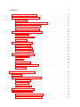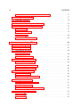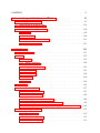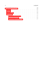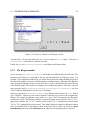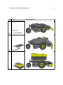
1
Webots User Guide
release 4.0.27
c 2002 Cyberbotics Ltd. All rights reserved.
copyright www.cyberbotics.com
December 3, 2004
2
c 2002 Cyberbotics Ltd. All rights reserved.
copyright All rights reserved
Permission to use, copy and distribute this documentation for any purpose and without fee is
hereby granted in perpetuity, provided that no modifications are performed on this documentation.
The copyright holder makes no warranty or condition, either expressed or implied, including
but not limited to any implied warranties of merchantability and fitness for a particular purpose,
regarding this manual and the associated software. This manual is provided on an as-is basis.
Neither the copyright holder nor any applicable licensor will be liable for any incidental or consequential damages.
This software was initially developed at the Laboratoire de Micro-Informatique (LAMI) of the
Swiss Federal Institute of Technology, Lausanne, Switzerland (EPFL). The EPFL makes no warranties of any kind on this software. In no event shall the EPFL be liable for incidental or
consequential damages of any kind in connection with use and exploitation of this software.
Trademark information
AiboTM is a registered trademark of SONY Corp.
GeForceTM is a registered trademark of nVidia, Corp.
JavaTM is a registered trademark of Sun MicroSystems, Inc.
KheperaTM and KoalaTM are registered trademarks of K-Team S.A.
LinuxTM is a registered trademark of Linus Torwalds.
Mac OS XTM is a registered trademark of Apple Inc.
MindstormsTM and LEGOTM are registered trademarks of the LEGO group.
PentiumTM is a registered trademark of Intel Corp.
Red HatTM is a registered trademark of Red Hat Software, Inc.
Visual C++TM , WindowsTM , Windows 95TM , Windows 98TM , Windows METM , Windows NTTM ,
Windows 2000TM and Windows XPTM are registered trademarks of Microsoft Corp.
UNIXTM is a registered trademark licensed exclusively by X/Open Company, Ltd.
Foreword
Webots is a three-dimensional mobile robot simulator. It was originally developed as a research
tool for investigating various control algorithms in mobile robotics.
This user guide will get you started using Webots. However, the reader is expected to have a
minimal knowledge in mobile robotics, in C, C++ or Java programming and in VRML97 (Virtual
Reality Modeling Language).
Webots 4 includes a physics engine allowing the user to define complex mobile robots with
various locomotion schemes (wheeled robots, legged robots or even flying robots). Predefined
sensors and actuators (like distance sensors, cameras, servos, grippers, etc.) allow the user to
model and simulate any mobile robot.
If you have already developed programs using Webots 3, please read chapter 2 to update your
programs to run with the new version.
We hope that you will enjoy working with Webots 4.
3
4
Thanks
Cyberbotics is grateful to all the people who contributed to the development of Webots, Webots
sample applications, the Webots User Guide, the Webots Reference Manual, and the Webots
web site, including Jordi Porta, Emanuele Ornella, Yuri Lopez de Meneses, Auke-Jan Ijspeert,
Alcherio Martinoli, Gerald Foliot, Allen Johnson, Michael Kertesz, Aude Billiard, and many
others.
Moreover, many thanks are due to Prof. J.-D. Nicoud (LAMI-EPFL) and Dr. F. Mondada for
their valuable support.
Finally, thanks to Skye Legon, who proof-readed this guide.
5
6
Contents
1
Installing Webots
1.1
Hardware requirements . . . . . . . . . . . . . . . . . . . . . . . . . . . . . . . 13
1.2
Installation procedure . . . . . . . . . . . . . . . . . . . . . . . . . . . . . . . . 13
1.3
2
1.2.1
RedHat Linux i386 . . . . . . . . . . . . . . . . . . . . . . . . . . . . . 13
1.2.2
Windows 95, 98, ME, NT, 2000 and XP . . . . . . . . . . . . . . . . . . 14
1.2.3
Mac OS X, version 10.2.8 . . . . . . . . . . . . . . . . . . . . . . . . . 14
Registration Procedure . . . . . . . . . . . . . . . . . . . . . . . . . . . . . . . 15
1.3.1
Webots license . . . . . . . . . . . . . . . . . . . . . . . . . . . . . . . 15
1.3.2
Registering . . . . . . . . . . . . . . . . . . . . . . . . . . . . . . . . . 16
Upgrading from Webots 3
2.1
2.2
3
13
19
Controller . . . . . . . . . . . . . . . . . . . . . . . . . . . . . . . . . . . . . . 19
2.1.1
Controller includes . . . . . . . . . . . . . . . . . . . . . . . . . . . . . 19
2.1.2
Controller library . . . . . . . . . . . . . . . . . . . . . . . . . . . . . . 19
2.1.3
Basic data type . . . . . . . . . . . . . . . . . . . . . . . . . . . . . . . 19
2.1.4
Khepera . . . . . . . . . . . . . . . . . . . . . . . . . . . . . . . . . . . 20
2.1.5
GTK+ GUI . . . . . . . . . . . . . . . . . . . . . . . . . . . . . . . . . 20
World . . . . . . . . . . . . . . . . . . . . . . . . . . . . . . . . . . . . . . . . 20
Getting Started with Webots
3.1
23
Introduction to Webots . . . . . . . . . . . . . . . . . . . . . . . . . . . . . . . 23
3.1.1
What is Webots ? . . . . . . . . . . . . . . . . . . . . . . . . . . . . . . 23
3.1.2
What can I do with Webots ? . . . . . . . . . . . . . . . . . . . . . . . . 23
3.1.3
What do I need to use Webots ? . . . . . . . . . . . . . . . . . . . . . . 24
7
8
CONTENTS
3.2
3.3
3.4
3.5
4
3.1.4
What is a world ? . . . . . . . . . . . . . . . . . . . . . . . . . . . . . . 25
3.1.5
What is a controller ? . . . . . . . . . . . . . . . . . . . . . . . . . . . . 25
Launching Webots . . . . . . . . . . . . . . . . . . . . . . . . . . . . . . . . . 25
3.2.1
On Linux . . . . . . . . . . . . . . . . . . . . . . . . . . . . . . . . . . 25
3.2.2
On Mac OS X . . . . . . . . . . . . . . . . . . . . . . . . . . . . . . . . 26
3.2.3
On Windows . . . . . . . . . . . . . . . . . . . . . . . . . . . . . . . . 26
Main Window: Menus and buttons . . . . . . . . . . . . . . . . . . . . . . . . . 26
3.3.1
File menu and shortcuts . . . . . . . . . . . . . . . . . . . . . . . . . . .
26
3.3.2
Edit menu . . . . . . . . . . . . . . . . . . . . . . . . . . . . . . . . . .
28
3.3.3
Simulation menu and the simulation buttons . . . . . . . . . . . . . . . .
29
3.3.4
Wizard menu . . . . . . . . . . . . . . . . . . . . . . . . . . . . . . . .
30
3.3.5
Help menu
3.3.6
Navigation in the scene . . . . . . . . . . . . . . . . . . . . . . . . . . . 31
3.3.7
Moving a solid object . . . . . . . . . . . . . . . . . . . . . . . . . . . . 32
3.3.8
Selecting a solid object . . . . . . . . . . . . . . . . . . . . . . . . . . . 32
. . . . . . . . . . . . . . . . . . . . . . . . . . . . . . . . . 31
Scene Tree Window . . . . . . . . . . . . . . . . . . . . . . . . . . . . . . . . . 32
3.4.1
Buttons of the Scene Tree Window . . . . . . . . . . . . . . . . . . . . . 33
3.4.2
VRML97 nodes . . . . . . . . . . . . . . . . . . . . . . . . . . . . . . . 34
3.4.3
Webots specific nodes . . . . . . . . . . . . . . . . . . . . . . . . . . . 36
3.4.4
Principle of the collision detection . . . . . . . . . . . . . . . . . . . . . 36
3.4.5
Writing a Webots file in a text editor . . . . . . . . . . . . . . . . . . . . 36
Citing Webots . . . . . . . . . . . . . . . . . . . . . . . . . . . . . . . . . . . . 37
3.5.1
Citing Cyberbotics’ web site . . . . . . . . . . . . . . . . . . . . . . . . 38
3.5.2
Citing a reference journal paper about Webots . . . . . . . . . . . . . . . 38
Tutorial: Modeling and simulating your robot
4.1
39
My first world: kiki.wbt . . . . . . . . . . . . . . . . . . . . . . . . . . . . . . . 39
4.1.1
Setup . . . . . . . . . . . . . . . . . . . . . . . . . . . . . . . . . . . . 39
4.1.2
Environment . . . . . . . . . . . . . . . . . . . . . . . . . . . . . . . . 40
4.1.3
Robot . . . . . . . . . . . . . . . . . . . . . . . . . . . . . . . . . . . . 44
4.1.4
A simple controller . . . . . . . . . . . . . . . . . . . . . . . . . . . . . 54
9
CONTENTS
4.2
Adding a camera to the kiki robot . . . . . . . . . . . . . . . . . . . . . . . . . . 55
4.3
Adding physics to the kiki simulation . . . . . . . . . . . . . . . . . . . . . . . . 55
4.4
4.5
4.6
5
4.3.1
Overview . . . . . . . . . . . . . . . . . . . . . . . . . . . . . . . . . . 55
4.3.2
Preparing the floor for a physics simulation . . . . . . . . . . . . . . . . 57
4.3.3
Adding physics to the kiki robot . . . . . . . . . . . . . . . . . . . . . . 57
4.3.4
Adding a ball in the kiki world . . . . . . . . . . . . . . . . . . . . . . . 57
Modelling an existing robot: pioneer2.wbt . . . . . . . . . . . . . . . . . . . . . 58
4.4.1
Environment . . . . . . . . . . . . . . . . . . . . . . . . . . . . . . . . 58
4.4.2
Robot with 16 sonars . . . . . . . . . . . . . . . . . . . . . . . . . . . . 58
4.4.3
Controller . . . . . . . . . . . . . . . . . . . . . . . . . . . . . . . . . . 65
Transfer to your own robot . . . . . . . . . . . . . . . . . . . . . . . . . . . . . 65
4.5.1
Remote control . . . . . . . . . . . . . . . . . . . . . . . . . . . . . . . 66
4.5.2
Cross-compilation . . . . . . . . . . . . . . . . . . . . . . . . . . . . . 68
4.5.3
Interpreted language . . . . . . . . . . . . . . . . . . . . . . . . . . . . 68
Adding custom ODE physics . . . . . . . . . . . . . . . . . . . . . . . . . . . . 69
4.6.1
Introduction . . . . . . . . . . . . . . . . . . . . . . . . . . . . . . . . . 69
4.6.2
Files . . . . . . . . . . . . . . . . . . . . . . . . . . . . . . . . . . . . . 69
4.6.3
Implementation . . . . . . . . . . . . . . . . . . . . . . . . . . . . . . . 69
4.6.4
Compiling the shared library . . . . . . . . . . . . . . . . . . . . . . . . 71
4.6.5
Example . . . . . . . . . . . . . . . . . . . . . . . . . . . . . . . . . . 71
Robot and Supervisor Controllers
73
5.1
Overview . . . . . . . . . . . . . . . . . . . . . . . . . . . . . . . . . . . . . . 73
5.2
Setting Up a Development Environment . . . . . . . . . . . . . . . . . . . . . . 73
5.2.1
Under Windows . . . . . . . . . . . . . . . . . . . . . . . . . . . . . . 73
5.2.2
Under Linux . . . . . . . . . . . . . . . . . . . . . . . . . . . . . . . . 75
5.2.3
Under Mac OS X . . . . . . . . . . . . . . . . . . . . . . . . . . . . . . 75
5.3
Setting Up a New Controller . . . . . . . . . . . . . . . . . . . . . . . . . . . . 75
5.4
Webots Execution Scheme . . . . . . . . . . . . . . . . . . . . . . . . . . . . . 76
5.4.1
From the controller’s point of view . . . . . . . . . . . . . . . . . . . . 76
5.4.2
From the point of view of Webots . . . . . . . . . . . . . . . . . . . . . 76
10
CONTENTS
5.4.3
6
Synchronous versus Asynchronous controllers . . . . . . . . . . . . . . 77
5.5
Reading Sensor Information . . . . . . . . . . . . . . . . . . . . . . . . . . . . 77
5.6
Controlling Actuators . . . . . . . . . . . . . . . . . . . . . . . . . . . . . . . . 78
5.7
Going further with the Supervisor Controller . . . . . . . . . . . . . . . . . . . . 78
5.8
Interfacing Webots to third party software . . . . . . . . . . . . . . . . . . . . . 79
5.8.1
Overview . . . . . . . . . . . . . . . . . . . . . . . . . . . . . . . . . . 79
5.8.2
Main advantages . . . . . . . . . . . . . . . . . . . . . . . . . . . . . . 79
5.8.3
Limitations . . . . . . . . . . . . . . . . . . . . . . . . . . . . . . . . . 80
5.8.4
MatLabTM TCP/IP utility . . . . . . . . . . . . . . . . . . . . . . . . . . 80
Tutorial: Using the KheperaTM robot
81
6.1
Hardware configuration . . . . . . . . . . . . . . . . . . . . . . . . . . . . . . . 81
6.2
Running the simulation . . . . . . . . . . . . . . . . . . . . . . . . . . . . . . . 82
6.3
Understanding the model . . . . . . . . . . . . . . . . . . . . . . . . . . . . . . 84
6.4
6.5
6.6
6.7
6.3.1
The 3D scene . . . . . . . . . . . . . . . . . . . . . . . . . . . . . . . . 84
6.3.2
The Khepera model . . . . . . . . . . . . . . . . . . . . . . . . . . . . . 85
Programming the Khepera robot . . . . . . . . . . . . . . . . . . . . . . . . . . 86
6.4.1
The controller program . . . . . . . . . . . . . . . . . . . . . . . . . . . 86
6.4.2
Looking at the source code . . . . . . . . . . . . . . . . . . . . . . . . . 86
6.4.3
Compiling the controller . . . . . . . . . . . . . . . . . . . . . . . . . . 89
Transferring to the real robot . . . . . . . . . . . . . . . . . . . . . . . . . . . . 89
6.5.1
Remote control . . . . . . . . . . . . . . . . . . . . . . . . . . . . . . . 89
6.5.2
Cross-compilation and upload . . . . . . . . . . . . . . . . . . . . . . . 90
Working extension turrets . . . . . . . . . . . . . . . . . . . . . . . . . . . . . . 91
6.6.1
The K213 linear vision turret . . . . . . . . . . . . . . . . . . . . . . . . 91
6.6.2
The Gripper turret . . . . . . . . . . . . . . . . . . . . . . . . . . . . . 91
6.6.3
Custom turrets and Khepera protocol . . . . . . . . . . . . . . . . . . . 92
Support for other K-Team robots . . . . . . . . . . . . . . . . . . . . . . . . . . 93
6.7.1
KoalaTM . . . . . . . . . . . . . . . . . . . . . . . . . . . . . . . . . . . 93
6.7.2
AliceTM . . . . . . . . . . . . . . . . . . . . . . . . . . . . . . . . . . . 95
11
CONTENTS
7
8
Tutorial: Using the LEGO MindstormsTM robots
97
7.1
Building up the Rover robot . . . . . . . . . . . . . . . . . . . . . . . . . . . . 97
7.2
Webots model of the Rover robot . . . . . . . . . . . . . . . . . . . . . . . . . . 119
7.3
Transfering to the real Rover robot . . . . . . . . . . . . . . . . . . . . . . . . . 120
7.3.1
leJOS . . . . . . . . . . . . . . . . . . . . . . . . . . . . . . . . . . . . 120
7.3.2
Installation . . . . . . . . . . . . . . . . . . . . . . . . . . . . . . . . . 120
7.3.3
Cross-compilation and upload . . . . . . . . . . . . . . . . . . . . . . . 121
7.3.4
How does it work ? . . . . . . . . . . . . . . . . . . . . . . . . . . . . . 121
ALife Contest
123
8.1
Previous Editions . . . . . . . . . . . . . . . . . . . . . . . . . . . . . . . . . . 123
8.2
Rules . . . . . . . . . . . . . . . . . . . . . . . . . . . . . . . . . . . . . . . . 123
8.2.1
Subject . . . . . . . . . . . . . . . . . . . . . . . . . . . . . . . . . . . 123
8.2.2
Robot Capabilities . . . . . . . . . . . . . . . . . . . . . . . . . . . . . 124
8.2.3
Programming Language . . . . . . . . . . . . . . . . . . . . . . . . . . 125
8.2.4
Scoring Rule . . . . . . . . . . . . . . . . . . . . . . . . . . . . . . . . 125
8.2.5
Participation . . . . . . . . . . . . . . . . . . . . . . . . . . . . . . . . 126
8.2.6
Schedule . . . . . . . . . . . . . . . . . . . . . . . . . . . . . . . . . . 126
8.2.7
Prize . . . . . . . . . . . . . . . . . . . . . . . . . . . . . . . . . . . . 126
8.3
Web Site . . . . . . . . . . . . . . . . . . . . . . . . . . . . . . . . . . . . . . . 126
8.4
How to Enter the Contest . . . . . . . . . . . . . . . . . . . . . . . . . . . . . . 127
8.5
8.4.1
Obtaining the software . . . . . . . . . . . . . . . . . . . . . . . . . . . 127
8.4.2
Running the software . . . . . . . . . . . . . . . . . . . . . . . . . . . . 128
8.4.3
Creating your own robot controller . . . . . . . . . . . . . . . . . . . . . 128
8.4.4
Submitting your controller to the ALife contest . . . . . . . . . . . . . . 129
8.4.5
Analysing the performance and improving your competing controller . . 130
Developers’ Tips and Tricks . . . . . . . . . . . . . . . . . . . . . . . . . . . . 132
8.5.1
Practical issues . . . . . . . . . . . . . . . . . . . . . . . . . . . . . . . 132
8.5.2
Java Security Manager . . . . . . . . . . . . . . . . . . . . . . . . . . . 132
8.5.3
Levels of Intelligence . . . . . . . . . . . . . . . . . . . . . . . . . . . . 133
12
9
CONTENTS
Practical Work: Robot Soccer
135
9.1
Setup . . . . . . . . . . . . . . . . . . . . . . . . . . . . . . . . . . . . . . . . 135
9.2
Rules . . . . . . . . . . . . . . . . . . . . . . . . . . . . . . . . . . . . . . . . 136
9.3
Programming . . . . . . . . . . . . . . . . . . . . . . . . . . . . . . . . . . . . 136
9.4
Extensions . . . . . . . . . . . . . . . . . . . . . . . . . . . . . . . . . . . . . . 136
9.4.1
Modifiying the soccer field . . . . . . . . . . . . . . . . . . . . . . . . . 137
9.4.2
Modifying the robots . . . . . . . . . . . . . . . . . . . . . . . . . . . . 137
9.4.3
Modifying the match supervisor . . . . . . . . . . . . . . . . . . . . . . 137
Chapter 1
Installing Webots
1.1
Hardware requirements
Webots is available for RedHat Linux i386, Mac OS X, Windows 95, Windows 98, Windows
ME, Windows NT, Windows 200 and Windows XP. Other versions of Webots for other UNIX
systems (Debian Linux i386, Solaris, Linux PPC, Irix) may be available upon request.
OpenGL hardware acceleration is supported on Windows, Mac OS X and in some Linux configurations. It may also be available on other UNIX systems.
1.2
Installation procedure
To install Webots, you must follow the instructions corresponding to your computer / operating
system listed below:
1.2.1 RedHat Linux i386
Webots will run on RedHat Linux distributions, starting from RedHat 7.2. Webots may run on
other Linux distributions. For example, it can be easily installed on Debian Linux, using the
alien command to translate the rpm package into a deb package before installation. If you do
use Red Hat Linux, please refer to your Linux distribution documentation to get the Webots rpm
package installed.
1. Log on as root
2. Insert the Webots CD-ROM, mount it (this might be automatic) and install the following
packages
13
14
CHAPTER 1. INSTALLING WEBOTS
mount /mnt/cdrom
cd /mnt/cdrom/linux
rpm -Uvh lib/mjpegtools-1.6.2-1.i386.rpm
# mjpegtools is useful to create MPEG movies from simulations
rpm -Uvh webots/webots-4.0.27-1.i386.rpm
rpm -Uvh webots/webots-kros-1.1.0-1.i386.rpm
# webots-kros is useful only if you want to cross-compile
# controllers for the Khepera robot
You may need to use the --nodeps or the --force if rpm fails to install the packages.
1.2.2 Windows 95, 98, ME, NT, 2000 and XP
1. Uninstall any previous release of Webots or Webots-kros, if any, from the Start menu,
Control Panel, Add / Remove Programs. or from the Start menu, Cyberbotics, Uninstall
Webots or Uninstall Webots-kros.
2. Insert the Webots CD-ROM and open it.
3. Go to the windows\webots directory on the CD-ROM.
4. Double click on the webots-4.0.27 setup.exe file.
5. Follow the installation instructions.
6. Optionally, double click on the webots-kros-1.1.0 setup.exe file to install the crosscompiler for the Khepera robots.
In order to be able to compile controllers, you will need to install a C/C++ development environment. We recommend to use Dev-C++ which is provided on the Webots CD-ROM (in the
windows/utils directory) as well as from the Bloodshed.net1 web site. Dev-C++ is an integrated development environment (IDE) for C/C++ with syntax highlighting running on Windows.
It includes the MinGW distribution with the GNU GCC compiler and utilities. This software is
distributed under the terms of the GNU public license and hence is free of charge.
You may also choose to use Microsoft Visual C++TM if you own a license of this software.
1.2.3
Mac OS X, version 10.2.8
1. Insert the Webots CD-ROM and open it.
2. Go to the mac:webots directory on the CD-ROM.
1
http://www.bloodshed.net
1.3. REGISTRATION PROCEDURE
15
3. Double click on the webots-4.0.27.dmg file.
4. This will mount on the desktop a volume named Webots containing the Webots folder.
Move this folder to your applications directory or wherever you would like to install Webots.
In order to be able to compile controllers, you will need to install the Apple Mac OS X Developer tools, included in the Mac OS X installation CD-ROMs. File editing and compilation
using Webots Makefiles can be achieved through these Apple tools. You will probably use the
Project Builder application to edit the source codes of the Webots controllers and the Terminal
application for invoking make from the directory in which your controller gets compiled.
If you would like to be able to create MPEG movies from your Webots simulations, you will
have to install the mjpegtools package. This package is located in the linux:lib directory of
the CD-ROM. Install it from the jpegtools-1.6.2.tar.gz tar ball. After installation, you
should be able to call mpeg2enc from the command line.
The CodeWarriorTM development environment is not supported for the development of controllers (although it may also work).
1.3
1.3.1
Registration Procedure
Webots license
Starting with Webots 4, a new license system has been introduced to facilitate the use of Webots.
When installing Webots, you will get a license file, called webots.key, containing your name,
address, serial number and computer ID. This encrypted file will enable you to use Webots according to the license you purchased. This file is strictly personal: you are not allowed to provide
copies of it to any third party in any way, including publishing that file on any Internet server
(web, ftp, or any other server). Any copy of your license file is under your responsibility. If a
copy of your license file is used by an unauthorized third party to run Webots, then Cyberbotics
may engage legal procedures against you. Webots licenses are (1) non-transferable and (2) nonexclusive. This means that (1) you cannot sell or give your Webots license to any third party, and
(2) Cyberbotics and its official Webots resellers may sell or give Webots licenses to third parties.
If you need further information about license issues, please send an e-mail to:
<[email protected]>
Please read your license agreement carefully before registering. This license is provided within
the software package. By using the software and documentation, you agree to abide by all the
provisions of this license.
16
CHAPTER 1. INSTALLING WEBOTS
1.3.2 Registering
After installing Webots, you will need to register your copy of Webots to get a license file called
webots.key allowing you to use all the features of Webots corresponding to the license you
purchased.
Regular webots.key license files are tied to a specific computer, making it impossible to use
Webots on another computer. However, if for some reason, you would like to move your Webots
license from a computer to another, just send us an e-mail at <[email protected]>
to explain the problem. If you plan to use several Webots licenses over a large number of computers, you should probably ask us to use the floating license server (see below for details).
Otherwise, you can jump to the simple registration subsection.
Floating license server: lserv
If you don’t want your Webots license file to be tied to specific computers, you have the option to
install a license server for Webots. This software, called lserv, allows you to run Webots concurrently on several machines defined by their IP addresses (or their names). Hence Webots is
not tied to a predefined number of machines but can be run on an unlimited number of computers.
However, the license server takes care that the number of computers running Webots simultaneously doesn’t exceed the maximum allowed by the license file. lserv should be installed on a
server machine, i.e., a computer that is on when users are supposed to run Webots.
Currently, lserv only runs on the Linux operating system. However, it allows Webots execution on Linux, Windows and Mac OS X machines. You need to provide Cyberbotics with
the MAC address of the eth0 network card of the Linux server running lserv so that a special webots.key license file can be created and will be sent to you. To know this MAC address, simply issue ifconfig eth0 as root and read the HWaddr parameter. It looks like:
00:50:04:1E:0E:38. Then, you will need to configure the server and clients to setup the
floating license server for your local network.
lserv is freely available from Cyberbotics at no extra cost upon simple request at:
<[email protected]>
Please follow the simple registration procedure to provide Cyberbotics with all the information
necessary to create the webots.key license file for lserv. The computer ID provided should
be the MAC address of your Linux server on which lserv will be running.
Simple registration
In order to proceed, launch Webots on the computer on which you would like to install the license
file. Go the Register menu item of the Help menu of Webots and follow the instructions. If this
computer is connected to the Internet, everything will run smoothly, fill in the requested form
and you will shortly receive the webots.key license file via e-mail. Otherwise, you will have
1.3. REGISTRATION PROCEDURE
17
to fill in a form2 on the website of Cyberbotics (see figure 1.1). You will then receive an e-mail
containing the webots.key file corresponding to your license.
Figure 1.1: Webots registration page
Please take care to properly fill in each field of this form. The Serial Number is the serial number
of your Webots package which is printed the CD-ROM under the heading S/N:. The computer
ID is given by Webots in the Register menu item of the Help menu.
After completing this form, click on the Submit button. You will receive shortly thereafter an
e-mail containing your personal license file webots.key which is needed to install a registered
copy of Webots as described below.
2
http://www.cyberbotics.com/registration/webots4.html
18
CHAPTER 1. INSTALLING WEBOTS
Registering several computers
If you need to register several computers, it may be convenient to register all the computers in
the same webots.key license file. Hence this unique license file could be copied across all the
computers needing a Webots license.
In order to proceed, just enter several computer IDs on the web form, corresponding to all the
computers you want to register. The computer IDs have to be seperated by a simple space character.
Copying the license file
Once you received it by e-mail, just copy the webots.key license file into the resources
directory of your Webots installation.
Under Linux, copy your personal webots.key file into the /usr/local/webots/resources
directory where Webots was just installed.
Under Mac OS X, copy your personal webots.key file into the Webots:resources directory
where Webots was just installed.
Under Windows, copy your personal webots.key file into the directory where Webots was just
installed, which is usually C:\Program Files\Webots\resources.
Chapter 2
Upgrading from Webots 3
If you have already worked with Webots 3, your existing programs may need to be modified for
use with Webots 4.
2.1
Controller
2.1.1 Controller includes
The include path of the device files is the same as in Webots 3.2, i.e.:
#include <device/robot.h>
#include <device/differential_wheels.h>
#include <device/distance_sensor.h>
2.1.2 Controller library
The name of the controller library to which you will link your executable files changed to ”Controller.dll” on Windows and ”libController.so” on Linux. It is not any more ”GtkController.dll”
or ”libGtkController.so”. Please update your project files or make files appropriately.
2.1.3 Basic data type
Since GTK+ and glib are not used any more, the data type coming from the glib are not recognized any more. Webots 4 uses the more standard C data types. Moreover, a couple of other
Webots specific data type have slightly changed to become more consistant with the rest of the
API. Please replace the following data types in your programs:
19
20
CHAPTER 2. UPGRADING FROM WEBOTS 3
Webots 3
gchar
guchar
guint8
gint8
gint
guint
gint32
guint32
gint16
guint16
gfloat
gdouble
gpointer
device tag
node ref
Webots 4
char
unsigned char
unsigned char
char
int
unsigned int
int
unsigned int
short
unsigned short
float
double
void *
DeviceTag
NodeRef
Table 2.1: Data types changes between Webots 3 and Webots 4
2.1.4 Khepera
If you developed controllers specifically for the Khepera robot, the khepera live function
should be replaced by robot live. Moreover, the #include <transfer/khepera.h>
should be removed. Please check also that the model field of the DifferentialWheels node
corresponding to the Khepera robot is ”Khepera” or ”Khepera II”, so that it will be automatically
recognized by Webots as a Khepera controller for remote control and code upload.
2.1.5
GTK+ GUI
The GTK+ graphical user interface is not any more integrated within the controller library.
Hence, you are free to use any graphical user interface library, like wxWindows, GTK+, Motif, MFC, etc. To use for example GTK+, you have two options: (1) you can perform all the
graphical user interface operations inside a separate thread, or (2) you can setup the GUI in the
same thread and call repeatly the gtk main iteration do function inside the main loop. An
example of using wxWindows as the GUI of a controller in provided in the wxgui controller
sample.
2.2
World
Very few changes were introduced in the Webots worlds that breaks the compatibility. However, since Webots 4 uses a different collision detection engine, boundingObject made up of
2.2. WORLD
21
Extrusion or IndexedFaceSet have to be changed to composite objects made up of Box,
Sphere and / or Cylinder. A composite object is a Group node containing Transform nodes
as children. These Transform nodes should contain the primitive shapes previously enumerated
and positioned appropriately.
22
CHAPTER 2. UPGRADING FROM WEBOTS 3
Chapter 3
Getting Started with Webots
To run a simulation in Webots, you need three things:
This chapter gives an overview of the basics of Webots, including the display of the world in the
main window and the structure of the .wbt file appearing in the scene tree window.
Robot and Supervisor controllers will be explained in detail in chapter 5.
3.1
Introduction to Webots
3.1.1 What is Webots ?
Webots is a professional mobile robot simulation software. It contains a rapid prototyping tool
allowing the user to create 3D virtual worlds with physics properties, such as mass repartition,
joints, friction coefficients, etc. The user can add simple inert objects or active objects called
mobile robots. These robots can have different locomotion schemes (wheeled robots, legged
robots or flying robots). Moreover, they be equipped with a number of sensor and actuator
devices, like distance sensors, motor wheels, cameras, servos, touch sensors, grippers, emitters,
receivers, etc. Finally the user can program each robot individually to exhibit a desired behavior.
Webots contains a large number of robot models and controller program examples that help the
users get started.
Webots also contains a number of interfaces to real mobiles robots, so that once your simulated
robot behaves as expected, you can transfer its control program to a real robot like Khepera,
Hemisson, LEGO Mindstorms, Aibo, etc.
3.1.2 What can I do with Webots ?
Webots is well suited for research and education projects related to mobile robotics. Many mobile
robotics projects have been relying on Webots for years in the following areas:
23
24
CHAPTER 3. GETTING STARTED WITH WEBOTS
• Mobile robot prototyping (academic research, automotive industry, aeronautics, vaccum
cleaner industry, toy industry, hobbyism, etc.)
• Multi-agent research (swarm intelligence, collaborative mobile robots groups, etc.)
• Adaptive behavior research (Genetic evolution, neural networks, adaptive learning, AI,
etc.).
• Mobile robotics teaching (robotics lectures, C/C++/Java programming lectures, robotics
contest, etc.)
3.1.3
What do I need to use Webots ?
To use Webots, you will need the following hardware:
• A fairly recent PC or Macintosh computer. We recommand at least a Pentium or PowerPC
CPU cadenced at 500Mhz. Webots works fine on desktop as well as laptop computers.
• A 3D capable graphics card, with at least 16MB RAM video memory. We recommand
nVidia graphics card for PC/Linux users. ATI graphics card are also well suited for Microsoft Windows and Apple Mac OS operating systems.
The following operating system are supported:
• Linux. Although only RedHat Linux is officially supported, Webots is known to run on
most major Linux distribution, including Mandrake, Debian, SuSE, Slackware, etc. We
recommand however to use a fairly recent recent version of Linux. Webots is provided as
an RPM package, as well as a DEB package.
• Windows. Although Webots runs on Windows 98, ME and NT4, we recommand to use a
recent version of Windows (like Windows 2003, Windows XP or Windows 2000) to avoid
minor issues.
• Mac OS X. Version 10.2 of Mac OS X or ealier is highly recommanded, as Webots hasn’t
been tested on older versions of Mac OS X and may not work as expected on such old
versions.
Usually, you will need to be administrator to be able to install Webots. Once installed, Webots
can be used as a regular unpriviliged user.
Although no special knowledge is needed to simply view the demos of robot simulations in
Webots, you will need a minimal amount of scientifical and technical knowledge to be able to
develop your own simulations:
3.2. LAUNCHING WEBOTS
25
• A basic knowledge of C, C++ or Java programming languages is necessary to program
your own robot controllers efficiently. However, even if you don’t know these languages,
you can still program the Hemisson robot using a simple graphical programming language
called BotStudio.
• If you don’t want to use existing robot models provided within Webots and would like
to create your own robot models, or add special objects in the simulated environments,
you will need some very basic knowledge of 3D computer graphics and VRML97 3D
description language. That will allow you to create 3D models in Webots or import them
from a 3D modelling software.
3.1.4
What is a world ?
A world in Webots is a 3D virtual environment in which you can create objects and robots. A
world is saved in the worlds directory, in a .wbt file which contains a description for any object:
Its position, orientation, geometry, appearance (like color, brightness), physical properties, type
of object, etc. A world is a hierarchical structure where objects can contain other objects (like
in VRML97). For example a robot can contain two wheels, a distance sensor and a servo which
itself contains a camera, thus making the camera moveable relatively to the robot thanks to the
servo. However, a world file does not contain all the information necessary to run a simulation.
The controller of each robot is specified in the world file by a reference to an executable binary
file, but the world file doesn’t contain this executable binary file.
3.1.5 What is a controller ?
A controller is an executable binary file which is used to control a robot described in a world file.
Controllers are stored in subdirectories of the Webots controllers directory. Controllers may
be native executables files (.exe under Windows) or Java binary files (.class).
3.2 Launching Webots
3.2.1 On Linux
From an X terminal, type webots to launch the simulator. You should see the world window
appear on the screen (see figure 3.1).
Webots can also run in batch mode, that is without displaying any window. This is useful to
launch simulations from scripts to perform extensive simulations with differents sets of parameters and save results automatically from a supervisor or robot controller process. To launch
Webots in batch mode, simply type webots --batch filename.wbt where filename.wbt is
26
CHAPTER 3. GETTING STARTED WITH WEBOTS
the name of the world file you want to use. Webots will then be launched in batch mode: The
speed of execution should correspond to the fast mode.
3.2.2 On Mac OS X
Open the directory in which you uncompressed the Webots package and double-click on the
Webots icon. You should see the world window appear on the screen (see figure 3.1).
3.2.3 On Windows
From the Start menu, go to the Program Files — Cyberbotics menu and click on the Webots 4.0.27
menu item. You should see the world window appear on the screen (see figure 3.1).
3.3
Main Window: Menus and buttons
The main window allows you to display your virtual worlds and robots described in the .wbt
file. Four menus and a number of buttons are available.
3.3.1
File
menu and shortcuts
The New menu item opens a new default world representing a chessboard of 10 x 10 plates on a
surface of 1 m x 1 m. The following button can be used as a shortcut:
New
The File menu will also allow you to perform the standard file operations: Open..., Save and Save
As..., respectively, to load, save and save with a new name the current world.
The following buttons can be used as shortcuts:
Open...
Save
The Revert item allows you to reload the most recently saved version of your .wbt file.
The following button can be used as a shortcut:
Revert
3.3. MAIN WINDOW: MENUS AND BUTTONS
27
Figure 3.1: Webots main window
The Export VRML item allows you to save the .wbt file as a .wrl file, conforming to the
VRML97 standard. Such a file can, in turn, be opened with any VRML97 viewer. This is
especially useful for publishing a world created with Webots on the Web.
The Make Animation... item allows you to create a 3D animation as a WVA file. This file format
is useful to playback Webots animations in real 3D, including navigation facilities. The WVA
viewer is called Webview. It is a freely available software downloadable from Cyberbotics’
Webview web site1 . It can run as a plugin for Internet Explorer, Netscape or Mozilla, but also as
a stand alone application. Webview works on Windows, Linux and Mac OS X. It is well suited
to demonstrate Webots results, possibly on the Internet World Wide Web.
The Make Movie... item allows you to create a MPEG-2 movie under Linux and Mac OS X or an
AVI movie under Windows. As movies are created on a 25 frame per second basis, you should
1
http://www.cyberbotics.com/webview
28
CHAPTER 3. GETTING STARTED WITH WEBOTS
adapt the basic simulation step and the refresh display parameters in the general preferences to
obtain a movie running at real time. Leaving the basic simulation step to 32 ms and setting the
refresh display each 1 basic simulation step should produce movies runnig faster than real time.
If you need exact real time, set the basic simulation step to 25 ms (it might then be optimal to
adapt your controllers’ robot step functions using a multiple value of 25, like 50, 75 or 100).
It is also possible to make accelerated movies by setting the refresh display each 2 (or more)
basic simulation step while leaving the basic time step to its original value (32 or 25).
The Screenshot... item allows you to take a screenshot of the current view in Webots. It opens a
file dialog to save the current view as a PNG image.
3.3.2
Edit
menu
The Scene Tree Window menu item opens the window in which you can edit the world and the
robot(s). A shortcut is available by double-clicking on a solid in the world. A solid is a physical
object in the world.
The Import VRML... menu item inserts VRML97 objects at the end of the scene tree. These objects
come from a VRML97 file you will have to specify. This feature is useful to import complex
shapes that were modeled in a 3D modelling software, then exported to VRML97 (or VRML
2.0), and then imported into Webots with this menu item. Most 3D modelling software, like 3D
Studio Max, Maya, AutoCAD or Art Of Illusion, include the VRML97 (or VRML 2.0) export
feature. Beware, Webots cannot import VRML 1.0 file format. Once imported, these objects
appear as Group, Transform or Shape nodes at the bottom of the scene tree. You can then
either turn these objects into Webots nodes (like Solid, DifferentialWheels, etc.) or cut
and paste them into the children list of existing Webots nodes.
The Restore Viewpoint menu item resets the camera position and orientation as it was originally
when the file was open. This feature is handy when you get lost while navigating in the scene
and want to return to the original camera position and orientation.
The Preferences item pops up a window with the following panels:
• General: The Startup mode allows you to choose the state of the simulation when Webots is launched (stop, run, fast; see the Simulation menu).
The Basic simulation step parameter defines the duration of the simulation step executed by Webots. It is expressed in milliseconds. Setting this value to a high value will
accelerate the simulation, but will decrease the accuracy of the simulation, especially for
physics simulation and collision detection This value is also used when the Step button is
pressed.
The Refresh display parameter is multiplicated to the basic step value to define how
frequently the 3D display of the main window is refreshed in normal Run mode.
• Rendering: This tab controls the 3D rendering in the simulation window.
3.3. MAIN WINDOW: MENUS AND BUTTONS
29
Checking the Display axes check box displays a red, green and blue axes representing
respectively the x, y and z axes of the world coordinate system.
Checking the Display sensor rays check box displays the distance sensor rays of the
robot(s) as red lines.
Checking the Display lights check box displays the lights (PointLight in the world
so that they can be moved more accurately).
• Files and paths: The user directory and the default .wbt world which is open when
launching Webots are defined here. The user directory should contain at least a worlds,
controllers, physics, and objects subdirectories where Webots will be looking for
files. A complete user directory can be created easily from the Setup user directory menu
item in the Wizard menu
3.3.3
Simulation
menu and the simulation buttons
In order to run a simulation a number of buttons are available corresponding to menu items found
under the Simulation menu:
Stop: Interrupt Run or Fast modes.
Step: Execute one simulation basic step. The duration of such a step is defined in the
preferences of Webots and can be adjusted to suit your needs.
Run: Execute simulation steps until the Stop mode is entered. In run mode, the 3D display
of the scene is refreshed every n basic step, where n is defined in the Webots preferences.
Fast: Same as Run, except that no display is performed (Webots PRO only). only.
The Fast mode performs a very fast simulation mode suited for heavy computation (genetic
algorithms, vision, learning, etc.). However, as the world display is disabled during a Fast simulation, the scene in the world window remains blank until the Fast mode is stopped. This feature
is available only with Webots PRO.
The World View / Robot View item allows you to switch between two different points of view:
• World View: This view corresponds to a fixed camera standing in the world.
• Robot View: This view corresponds to a mobile camera following a robot.
The default view is the world view. If you want to switch to the Robot View, first select the robot
you want to follow (click on the pointer button then on the robot), and then choose Robot View
in the Simulation menu. To return to the World View mode, reselect this item.
30
CHAPTER 3. GETTING STARTED WITH WEBOTS
A speedometer (see figure 3.2) allows you to observe the speed of the simulation on your computer. It is displayed in the bottom right hand side of the main window and indicates how fast the
simulation runs compared to real time. In other words, it represents the speed of the virtual time.
If the value of the speedometer is 2, it means that your computer simulation is running twice as
fast as the corresponding real robots would. This information is relevant both in Run mode and
Fast mode.
Figure 3.2: Speedometer
To the left of the speedometer, the virtual time is displayed using the following format: H:MM:SS:MMM
where H is the number of hours (may lie on several digits), MM is the number of minutes, SS is
the number of seconds and MMM is the number of milliseconds. (see figure 3.2). If the speedometer value is higher than one, the virtual time will be progressing faster than the real time. This
information is relevant both in Run mode and Fast mode.
The basic simulation time step can be chosen from the preferences window. It is expressed
in virtual time milliseconds. The value of this time step defines the duration of the time step
executed during the Step mode. This step is multiplicated by the refresh parameter to define how
frequently the display is refreshed. The refresh parameter can be changed from the preferences
window.
In Run mode, with a time step of 64 ms and a fairly simple world displayed with the default
window size, the speedometer will typically indicate approximately 0.5 on a Pentium II / 266
Mhz without hardware acceleration and 12 on a Pentium III / 500 Mhz with an nVidia Geforce
II MX graphics card.
3.3.4
Wizard
menu
The Wizard menu is useful to facilitate the creation of a new user directory (from the Setup user
directory menu item) or the creation of a new robot controller (from the New robot controller
menu item).
The Setup user directory menu item will ask you to choose a name for your user directory. A
user directory is a directory that will contain all the files you will create while using Webots,
including world file, controller files, object files, physics shared libraries, etc. Once you chose
a name for this user directory, you will be asked to choose a location on your hard disk where
to store it. Then, Webots will create this directory at the specified location and it will create all
3.3. MAIN WINDOW: MENUS AND BUTTONS
31
the subdirectories and files needed. Finally, it will set this directory as the current user directory
in the Webots preferences. From there, you will be able to save all your Webots files in the
subdirectories of this user directory (world files, controllers, etc.).
The New robot controller menu item allows you to create a new controller program for your robot.
You will be prompted to choose between a C, C++ or a Java controller. Then, Webots will ask
you the name of your controller and it will create all the necessary files (including a template
source code file) in your user directory.
3.3.5
Help
menu
In the Help menu, the About... item opens the About... window, displaying the license information.
The Introduction item is a short introduction to Webots (HTML file). You can access the User
Guide and the Reference Manual with the User Guide and Reference Manual items (PDF files).
The Web site of Cyberbotics item lets you visit our Web site.
3.3.6 Navigation in the scene
The view of the scene is generated by a virtual camera set in a given position and orientation.
You can change this position and orientation to navigate in the scene using the mouse buttons.
The x, y, z axes mentioned below correspond to the coordinate system of the camera; z is the axis
corresponding to the direction of the camera.
• Rotate viewpoint: To rotate the camera around the x and y axis, you have to set the mouse
pointer in the 3D scene, press the left mouse button and drag the mouse:
if you clicked on a solid object, the rotation will be centered around the origin of the local
coordinate system of this object.
if you clicked outside of any solid object, the rotation will be centered around the origin of
the world coordinate system.
• Translate viewpoint: To translate the camera in the x and y directions, you have to set the
mouse pointer in the 3D scene, press the right mouse button and drag the mouse.
• Zoom / Tilt viewpoint: Set the mouse pointer in the 3D scene, then:
if you press both left and right mouse buttons (or the middle button) and drag the mouse
vertically, the camera will zoom in or out.
if you press both left and right mouse buttons (or the middle button) and drag the mouse
horizontally, the camera will rotate around its z axis (tilt movement).
if you use the wheel of the mouse, the camera will zoom in or out.
32
CHAPTER 3. GETTING STARTED WITH WEBOTS
3.3.7 Moving a solid object
In order to move an object, hold the shift key down while using the mouse.
• Translation: Pressing the left mouse button while the shift key is pressed allows you to
drag solid objects on the ground (xz plan).
• Rotation: Pressing the right mouse button while the shift key is pressed rotates solid objects: A first click is necessary to select a solid object, then a second shift-press-and-drag
rotates the selected object around its y axis.
• Lift: Pressing both left and right mouse buttons, the middle mouse button, or rolling the
mouse wheel while the shift key is pressed allows you to lift up or down the selected solid
object.
3.3.8 Selecting a solid object
Simply clicking on a solid object allows you to select this object. Selecting a robot enables the
choice of Robot View in the simulation menu. Double-clicking on a solid object opens the scene
tree window where the world and robots can be edited. The selected solid object appears selected
in the scene tree window as well.
3.4
Scene Tree Window
As seen in the previous section, to access to the Scene Tree Window you can either choose Scene
Tree Window in the Edit menu, or click on the pointer button and double-click on a solid object.
The scene tree contains all information necessary to describe the graphic representation and simulation of the 3D world. A world in Webots includes one or more robots and their environment.
The scene tree of Webots is structured like a VRML97 file. It is composed of a list of nodes,
each containing fields. Fields can contain values (text string, numerical values) or nodes.
Some nodes in Webots are VRML97 nodes, partially or totally implemented, while others are
specific to Webots. For instance the Solid node inherits from the Transform node of VRML97
and can be selected and moved with the buttons in the World Window.
This section describes the buttons of the Scene Tree Window, the VRML97 nodes, the Webots
specific nodes and how to write a .wbt file in a text editor.
33
3.4. SCENE TREE WINDOW
Figure 3.3: Scene Tree Window
3.4.1 Buttons of the Scene Tree Window
The scene tree with the list of nodes appears on the left side of the window. Clicking on the + in
front of a node or double-clicking on the node displays the fields inside the node, and similarly
expands the fields. The field values can be defined on the top right side of the window. Five
editing buttons are available on the bottom right side of the window:
Cut
Copy
Paste after
These three buttons let you cut, copy and paste nodes and fields. However, you can’t perform
these operations on the first three nodes of the tree (WorldInfo, Viewpoint and Background).
These nodes are mandatory and cannot be duplicated. Similarly, you can’t copy the Supervisor
node because only one supervisor is allowed. Please note that when you cut or copy a robot node,
like a DifferentialWheels or Supervisor node, the controller field of this node is reset
to "void".
34
CHAPTER 3. GETTING STARTED WITH WEBOTS
Delete: This button allows you to delete a node. It appears only if a node is selected. If a
field is selected, the Default Value button appears instead.
Default Value: You can click on this button to reset a field to its default value(s). A field
with values must be selected in order to perform this button. If a node is selected, the Delete
button replaces it.
Transform: This button allows you to transform a node into another one.
Insert after: With this button, you can insert a node after the one currently selected. This
new node contains fields with default values, which you can of course modify to suit your needs.
This button also allows you to add a node to a children field. In all cases, the software only
permits you to insert a coherent node.
Insert Node: Use this to insert a node into a field whose value is a node. You can insert
only a coherent node.
Export Node: Use this button to export a node into a file. Usually, nodes are saved in your
objects directory. Such saved nodes can then be reused in other worlds.
Import Node: Use this button to import a previously saved node into the scene tree. Usually,
saved nodes are located in the Webots objects directory or in your own objects directory.
The Webots objects directory already contains a few nodes that can be easily imported.
3.4.2 VRML97 nodes
A number of VRML97 nodes are partially or completely supported in Webots.
The exact features of VRML97 are the subject of a standard managed by the International Standards Organization (ISO/IEC 14772-1:1997).
You can find the complete specifications of VRML97 on the official VRML97 Web site2 .
The following VRML97 nodes are supported in Webots:
• Appearance
• Background
2
http://www.web3d.org
3.4. SCENE TREE WINDOW
35
• Box
• Color
• Cone
• Coordinate
• Cylinder
• DirectionalLight
• ElevationGrid
• Fog
• Group
• ImageTexture
• IndexedFaceSet
• IndexedLineSet
• Material
• PointLight
• Shape
• Sphere
• Switch
• TextureCoordinate
• TextureTransform
• Transform
• Viewpoint
• WorldInfo
The Webots Reference Manual gives a list of nodes supported in Webots and specify which fields
are actually used. For a comprehensive description of the VRML97 nodes, please refer to the
VRML97 documentation.
36
CHAPTER 3. GETTING STARTED WITH WEBOTS
3.4.3 Webots specific nodes
In order to implement powerful simulations including mobile robots with different propulsion
schemes (wheeled robots, legged robots or flying robots), a number of nodes specific to Webots
have been added to the VRML97 set of nodes.
VRML97 uses a hierarchical structure for nodes. For example, the Transform node inherits
from the Group node, such that, like the Group node, the Transform node has a children
field, but it also adds three additional fields: translation, rotation and scale.
In the same way, Webots introduces new nodes which inherit from the VRML97 Transform
node, principally the Solid node. Other Webots nodes (DifferentialWheels, Camera,
TouchSensor, etc.) inherit from this Solid node.
The Reference Manual gives a complete description of all Webots nodes and their respective
fields.
3.4.4 Principle of the collision detection
The collision detection engine is able to detect a collision between two Solid nodes. It calculates
the intersection between the bounding objects of the solids. A bounding object (described in the
boundingObject field of the Solid node) is a geometric shape or a group of geometric shapes
which bounds the solid. If the boundingObject field is NULL, then no collision detection is
performed for this Solid node. A Solid node may contain other Solid nodes as children,
each of them having its own bounding object.
The collision detection is mainly used to detect if a robot (for example a DifferentialWheels
node) collides with an obstacle (Solid node), or with another robot. Two Solid nodes can never
inter-penetrate each other; their movement is stopped just before the collision.
Example: A solid with a bounding box different from its list of children.
Let us consider the Khepera robot model. It is not exactly a Solid node, but the principle for the
boundingObject is the same. Open the khepera.wbt file and look at the boundingObject
field of the DifferentialWheels node. The bounding object is a cylinder which has been
transformed. See figure 3.4.
3.4.5 Writing a Webots file in a text editor
It is possible to write a Webots world file (.wbt) using a text editor. A world file contains a
header, nodes containing fields and values. Note that only a few VRML97 nodes are implemented, and that there are nodes specific to Webots. Moreover, comments can only be written in
the DEF, and not like in a VRML97 file.
The Webots header is:
3.5. CITING WEBOTS
37
Figure 3.4: The bounding box of the Khepera robot
#VRML_SIM V4.0 utf8
After this header, you can directly write your nodes. The three nodes WorldInfo, Viewpoint
and Background are mandatory.
Note: We recommend that you write your file using the tree editor. However it may be easier to
make some particular modifications using a text editor (like using the search and replace feature
of a text editor).
3.5
Citing Webots
When writing a scientific paper, or describing your project involving Webots on a web site, it is
always appreciated to make a correct reference to Webots, mentionning Cyberbotics’ web site
explicitely and a reference journal paper describing Webots. In order to help you in such a task,
we provide here some citation examples, including BibTex entries that you can freely reuse in
your own documents:
38
CHAPTER 3. GETTING STARTED WITH WEBOTS
3.5.1 Citing Cyberbotics’ web site
This project uses Webots3 , a commercial mobile robot simulation software developed by Cyberbotics Ltd.
This project uses Webots (http://www.cyberbotics.com), a commercial mobile robot simulation
software developed by Cyberbotics Ltd.
The BibTex reference entry may look odd, as it is very different from a standard paper citation
and we want the specified fields to appear in the normal plain citation mode of LaTeX.
@MISC{Webots,
AUTHOR = {Webots},
TITLE = {http://www.cyberbotics.com},
NOTE
= {Commercial Mobile Robot Simulation Software},
EDITOR = {Cyberbotics Ltd.},
URL
= {http://www.cyberbotics.com}
}
Once compiled with LaTeX, it should display as follow:
References
[1] Webots. http://www.cyberbotics.com. Commercial Mobile Robot Simulation Software.
3.5.2 Citing a reference journal paper about Webots
A reference paper was published in the International Journal of Advanced Robotics Systems.
Here is the BibTex entry:
@ARTICLE{Webots04,
AUTHOR = {Michel, O.},
TITLE
= {Webots: Professional Mobile Robot Simulation},
JOURNAL = {Journal of Advanced Robotics Systems},
YEAR
= {2004},
VOLUME = {1},
NUMBER = {1},
PAGES
= {39--42},
URL
= {http://www.ars-journal.com/ars/SubscriberArea/Volume1/39-42.pdf}
}
3
http://www.cyberbotics.com
Chapter 4
Tutorial: Modeling and simulating your
robot
The aim of this chapter is to give you several examples of robots, worlds and controllers. The first
world is very simple, nevertheless it introduces the construction of any basic robot, and explains
how to program a controller. The second example shows you how to model and use a camera on
this simple robot. The third example will add physics to the robot and world, so that the robot can
play with a ball. Finally, the last example will show you how to build a virtual Pioneer 2TM robot
from ActivMedia Robotics.
4.1
My first world: kiki.wbt
As a first introduction, we are going to simulate a very simple robot made up of a box, two wheels
and two infra-red sensors (see figure 4.1). The robot is controlled by a program performing
obstacle avoidance inspired from Braitenberg’s algorithm. It evolves in a simple environment
surrounded by a wall.
4.1.1 Setup
Before starting, please check that Webots was installed properly on your computer (refer to the
installation chapter of this manuel). Then, you will have to setup a working directory that will
contain the files your will create in this tutorial. To do so, create a directory called my webots in
your local directory. Then, create a couple of subdirectories called worlds and controllers.
The first one will contain the simlation worlds you will create, while the second one will contain
your programs controlling the simulated robots. If you are using gcc as a compiler, you may
also need to copy the Makefile.include file from the Webots controllers directory in
your local controllers directory. To start up with this tutorial, simply copy the kiki.wbt
worlds from the Webots worlds directory to your local worlds directory. You will also have
39
40
CHAPTER 4. TUTORIAL: MODELING AND SIMULATING YOUR ROBOT
IR sensors
wheels
Figure 4.1: The kiki robot
to copy the kiki subdirectory which contains the kiki.png image. Finally, copy the simple
directory from the Webots controllers directory to your local controllers directory. Now
you should inform Webots that your working directory is there. To do it, launch Webots and
open the Preferences... from the Edit menu. Select the Files and paths tab and select your local
my webots directory as the User directory. You can also set the kiki.wbt world as the default
world. Then quit Webots, so that the preferences are saved. When you will restart it, it will run
the kiki world.
4.1.2 Environment
This very first simulated world is as simple as possible. It includes a floor and a surrounding
wall to avoid that the robot escapes. This wall is modelled using an Extrusion node. The
coordinates of the wall are shown in figure 4.2.
First, launch Webots and stop the current running simulation by pressing the Stop button. Go
to the File menu, New item to create a new world. This can also by achieved through the New
button, or the keyboard shortcut indicated in the File menu. Then open the scene tree window
from the Scene Tree... item in the Edit menu. This can also be achieved by double-clicking in the
3D world. Let us start by changing the lighting of the scene:
1. Select the PointLight node, and click on the + just in front of it. You can now see the
different fields of the PointLight node. Select ambientIntensity and enter 0.6 as a
value, then select intensity and enter 0.8, then select location and enter 0.5 0.5 0.5
as values. Press return.
2. Select the PointLight node, copy and paste it. Open this new PointLight node and
type -0.5 0.5 0.5 in the location field.
41
4.1. MY FIRST WORLD: KIKI.WBT
z
7
8
(x,z) coordinates:
4
3
x
1
6
5
0
2
0
1
2
3
4
5
6
7
8
9
(−0.489, −0.5)
(−0.489, −0.49)
(0.49, −0.49)
(0.49, 0.49)
(−0.49, 0.49)
(−0.49, −0.5)
(−0.5, −0.5)
(−0.5, 0.5)
(0.5, 0.5)
(0.5, −0.5)
9
Figure 4.2: The kiki world
3. Repeat this paste operation twice again with -0.5 0.5 -0.5 in the location field of the
third PointLight node, and 0.5 0.5 -0.5 in the location field of the fourth and last
PointLight node.
4. The scene is now better lit. Open the Preferences... from the Edit menu, select the Rendering tab and check the Display lights option. Click on the OK button to leave the preferences
and check that the light sources are now visible in the scene. Try the different mouse
buttons, including the mouse wheel if any, and drag the mouse in the scene to navigate
and observe the location of the light sources. If you need more explanations with the 3D
navigation in the world, go to the Help menu and select the How do I navigate in 3D ? item.
Secondly, let us create the wall:
1. Select the last Transform node in the scene tree window (which is the floor) and click on
the insert after button.
2. Choose a Solid node.
3. Open this newly created Solid node from the + sign and type ”wall” in its name field.
4. Select the children field and Insert after a Shape node.
42
CHAPTER 4. TUTORIAL: MODELING AND SIMULATING YOUR ROBOT
5. Open this Shape, select its apperance field and create an Appearance node from the
New node button. Use the same technique to create a Material node in the material
field of the Appearance node. Select the diffuseColor field of the Material node
and choose a color to define the color of the wall. Let us make it dark green.
6. Now create an Extrusion node in the geometry field of the Shape.
7. Set the convex field to FALSE. Then, set the wall corner coordinates in the crossSection
field as shown in figure 4.2. You will have to re-enter the first point (0) at the last position
(10) to complete the last face of the extrusion.
8. In the spine field, write that the wall ranges between 0 and 0.1 along the Y axis (instead
of the 0 and 1 default values).
9. As we want to prevent our robot to pass through the walls like a ghost, we have to define
the boundingObject field of the wall. Bounding objects cannot use complex geometry
objects. They are limited to box, cylinder and spheres primitives. Hence, we will have
to create four boxes (representing the four walls) to define the bounding object of the
surrouding wall. Select the boundingObject field of the wall and create a Group node
that will contain the four walls. In this Group, insert a Transform node as a children.
Create a Shape as the unique children of the Transform. Instead of creating a new
Appearance for this Shape, reuse the first Appearance you created (for the wall). To
do so, go back to the children list of the wall Solid, open the Shape, click on the
Appearance node and you will see on the right hand side of the window that you can enter
a DEF name. Write WALL APPEARANCE as a DEF name and return to the Shape of
the bounding object. Select its appearance field and create a New node for it. However,
in the Create a new node dialog, you will now be able to use the WALL APPEARANCE
you just defined. Select this item and click OK. Now create a Box as a geometry for this
Shape node. Set the size of the Box to [ 1 0.1 0.01 ], so that it matches the size of a
wall. Set the translation field of the Transform node to [ 0 0.05 0.495 ], so that it
matches the position of a wall. Now, close this Transform, copy and paste it as the second
children of the list. Set the translation field of the new node to [ 0 0.05 -0.495 ],
so that it matches the opposite wall. Repeat this operation with the two remaining walls
and set their rotation fields to [ 0 1 0 1.57 ] so that they match the orientation of the
corresponding walls. You also have to edit their translation field as well, so that they
match the position of the corresponding walls.
10. Close the tree editor, save your file as ”my kiki.wbt” and look at the result.
The wall in the tree editor is represented in figure 4.3, while the same wall in the world editor is
visible in figure 4.4
4.1. MY FIRST WORLD: KIKI.WBT
Figure 4.3: The wall in the tree editor
Figure 4.4: The wall in the world window
43
44
CHAPTER 4. TUTORIAL: MODELING AND SIMULATING YOUR ROBOT
4.1.3 Robot
This subsection describes how to model the kiki robot as a DifferentialWheels node containing several children: a Transform node for the body, two Solid nodes for the wheels, two
DistanceSensor nodes for the infra-red sensors and a Shape node with a texture.
The origin and the axis of the coordinate system of the robot and its dimensions are shown in
figure 4.5.
FRONT VIEW
y
LEFT SIDE VIEW
y
x
z
0.08
0.08
0.08
0.05
0.02
Ø 0.05
0.01
Figure 4.5: Coordinate system and dimensions of the kiki robot
To model the body of the robot:
1. Open the scene tree window.
2. Select the last Solid node.
3. Insert after a DifferentialWheels node, set its name to ”kiki”.
4.1. MY FIRST WORLD: KIKI.WBT
45
4. In the children field, first introduce a Transform node that will contain a shape with a
box. In the new children field, Insert after a Shape node. Choose a color, as described
previously. In the geometry field, insert a Box node. Set the size of the box to [0.08 0.08
0.08]. Now set the translation values to [ 0 0.06 0 ] in the Transform node (see figure
4.6)
Figure 4.6: Body of the kiki robot: a box
To model the left wheel of the robot:
1. Select the Transform node corresponding to the body of the robot and Insert after a
Solid node in order to model the left wheel. Type ”left wheel” in the name field, so that
this Solid node is recognized as the left wheel of the robot and will rotate according to
the motor command.
2. The axis of rotation of the wheel is x. The wheel will be made of a Cylinder rotated
of pi/2 radians around the z axis. To obtain proper movement of the wheel, you must pay
attention not to confuse these two rotations. Consequently, you must add a Transform
node to the children of the Solid node.
3. After adding this Transform node, introduce inside it a Shape with a Cylinder in its
geometry field. Don’t forget to set an appearance as explained previously. The dimensions of the cylinder should be 0.01 for the height and 0.025 for the radius. Set the
rotation to [ 0 0 1 1.57 ]. Pay attention to the sign of the rotation; if it is wrong, the
wheel will turn in the wrong direction.
4. In the Solid node, set the translation to [-0.045 0.025 0] to position the left wheel, and set
the rotation of the wheel around the x axis: [1 0 0 0].
46
CHAPTER 4. TUTORIAL: MODELING AND SIMULATING YOUR ROBOT
5. Give a DEF name to your Transform: WHEEL; notice that you positioned the wheel in
translation at the level of the Solid node, so that you can reuse the WHEEL Transform
for the right wheel.
6. Close the tree window, look at the world and save it. Use the navigation buttons to change
the point of view.
To model the right wheel of the robot:
1. Select the left wheel Solid node and insert after another Solid node. Type ”right wheel”
in the name field. Set the translation to [0.045 0.025 0] and the rotation to [1 0 0 0].
2. In the children, Insert after USE WHEEL. Press Return, close the tree window and save
the file. You can examine your robot in the world editor, move it and zoom in on it.
The robot and its two wheels are shown in figure 4.7 and figure 4.8.
Figure 4.7: Wheels of the kiki robot
The two infra-red sensors are defined as two cylinders on the front of the robot body. Their
diameter is 0.016 m and their height is 0.004 m. You must position these sensors properly so that
the sensor rays point in the right direction, toward the front of the robot.
4.1. MY FIRST WORLD: KIKI.WBT
47
Figure 4.8: Body and wheels of the kiki robot
1. In the children of the DifferentialWheels node, insert after a DistanceSensor
node.
2. Type the name ”ir0”. It will be used by the controller program.
3. Let’s attach a cylinder shape to this sensor: In the children list of the DistanceSensor
node, Insert after a Transform node. Give a DEF name to it: INFRARED, which you will
use for the second IR sensor.
4. In the children of the Transform node, insert after a Shape node. Define an appearance
and insert a Cylinder in the geometry field. Type 0.004 for the height and 0.008 for the
radius.
5. Set the rotation for the Transform node to [0 0 1 1.57] to adjust the orientation of the
cylinder.
6. In the DistanceSensor node, set the translation to position the sensor and its ray: [0.02
0.08 -0.042]. In the File menu, Preferences, Rendering, check the Display sensor rays box.
In order to have the ray directed toward the front of the robot, you must set the rotation to
[0 1 0 1.57].
48
CHAPTER 4. TUTORIAL: MODELING AND SIMULATING YOUR ROBOT
7. In the DistanceSensor node, you must introduce some values of distance measurements
of the sensors to the lookupTable field, according to figure 4.9. These values are:
lookupTable [ 0
0.05
0.15
1024
1024
0
0,
0,
0 ]
Measured
value
1024
0
0.05
0.15
Distance to
the wall
Figure 4.9: Distance measurements of the kiki sensors.
8. To model the second IR sensor, select the DistanceSensor node and Insert after a new
DistanceSensor node. Type ”ir1” as a name. Set its translation to [-0.02 0.08 -0.042]
and its rotation to [0 1 0 1.57]. In the children, insert after USE INFRARED. In the
lookupTable field, type the same values as shown above.
The robot and its two sensors are shown in figure 4.10 and figure 4.11.
Note: A texture can only be mapped on an IndexedFaceSet shape. The texCoord and
texCoordIndex entries must be filled. The image used as a texture must be a .png or a .jpg
file, and its size must be (2n ) * (2n ) pixels (for example 8x8, 16x16, 32x32, 64x64, 128x128 or
256x256 pixels). Transparent images are not allowed in Webots. Moreover, PNG images should
use either the 24 or 32 bit per pixel mode (lower bpp or gray levels are not supported). Beware
of the maximum size of texture images depending on the 3D graphics board you have: some old
3D graphics boards are limited to 256x256 texture images while more powerful ones will accept
2048x2048 texture images.
To paste a texture on the face of the robot:
1. Select the last DistanceSensor node and Insert after a Shape node.
49
4.1. MY FIRST WORLD: KIKI.WBT
Figure 4.10: The DistanceSensor nodes of the kiki robot
2. Create an Appearance node in the appearance field. Create an ImageTexture node in
the texture field of this node, with the following URL: "kiki/kiki.png". This refers
to an image file lying in the worlds directory.
3. In the geometry field, create an IndexedFaceSet node, with a Coordinate node in
the coord field. Type the coordinates of the points in the point field:
[ 0.015
0.015
-0.015
-0.015
0.05
0.03
0.03
0.05
-0.041,
-0.041,
-0.041,
-0.041 ]
and Insert after in the coordIndex field the following values: 0, 1, 2, 3, -1. The optional
-1 value is there to mark the end of the face. It is useful when defining several faces for the
same IndexedFaceSet node.
4. In the texCoord field, create a TexureCoordinate node. In the point field, enter the
coordinates of the texture:
50
CHAPTER 4. TUTORIAL: MODELING AND SIMULATING YOUR ROBOT
Figure 4.11: The kiki robot and its sensors
[ 0
1
1
0
0
0
1
1 ]
and in the texCoordIndex field, type 3, 0, 1, 2. This is the standard VRML97 way to
explain how the texture should be mapped to the object.
5. The texture values are shown in figure 4.12.
To finish with the DifferentialWheels node, you must fill in a few more fields:
1. In the controller field, type the name ”simple”. It is used to determine which controller
program controls the robot.
2. The boundingObject field can contain a Transform node with a Box, as a box as
a bounding object for collision detection is sufficient to bound the kiki robot. Create a
Transform node in the boundingObject field, with the translation set to [0 0.05
-0.002] and a Box node in its children. Set the dimension of the Box to [0.1 0.1 0.084].
4.1. MY FIRST WORLD: KIKI.WBT
51
Figure 4.12: Defining the texture of the kiki robot
3. In the axleLength field, enter the length of the axle between the two wheels: 0.09 (according to figure 4.5).
4. In the wheelRadius field, enter the radius of the wheels: 0.025.
5. Values for other fields are shown in figure 4.13 and the finished robot in its world is shown
in figure 4.14.
52
CHAPTER 4. TUTORIAL: MODELING AND SIMULATING YOUR ROBOT
Figure 4.13: The other fields of the DifferentialWheels node
4.1. MY FIRST WORLD: KIKI.WBT
Figure 4.14: The kiki robot in its world
53
54
CHAPTER 4. TUTORIAL: MODELING AND SIMULATING YOUR ROBOT
The kiki.wbt is included in the Webots distribution, in the worlds directory.
4.1.4 A simple controller
This first controller is very simple and thus named simple. The controller program simply reads
the sensor values and sets the two motors speeds, in such a way that kiki avoids the obstacles.
Below is the source code for the simple.c controller:
#include <device/robot.h>
#include <device/differential_wheels.h>
#include <device/distance_sensor.h>
#define SPEED 100
static DeviceTag ir0,ir1;
static void reset(void) {
ir0 = robot_get_device("ir0");
ir1 = robot_get_device("ir1");
// printf("ir0=134530819 ir1=1108551892\n",ir0,ir1);
distance_sensor_enable(ir0,64);
distance_sensor_enable(ir1,64);
}
static void run(int ms) {
short left_speed,right_speed;
unsigned short ir0_value,ir1_value;
ir0_value = distance_sensor_get_value(ir0);
ir1_value = distance_sensor_get_value(ir1);
if (ir1_value>200) {
left_speed = -20;
right_speed = 20;
} else if (ir0_value>200) {
left_speed = 20;
right_speed = -20;
} else {
left_speed =SPEED;
right_speed=SPEED;
}
/* Set the motor speeds */
differential_wheels_set_speed(left_speed,right_speed);
return 64; /* next call after 64 milliseconds */
}
4.2. ADDING A CAMERA TO THE KIKI ROBOT
55
int main() {
robot_live(reset);
robot_run(run); /* this function never returns */
return 0;
}
This controller lies in the simple directory of the Webots controllers directory.
4.2
Adding a camera to the kiki robot
This section can be considered as an exercice to check if you understood the principles for adding
devices to a robot. If you want to skip this section because you feel comfortable with Webots
and you are not interested in cameras, you may jump directly to the next section which addresses
physics and does not require that the kiki be equipped with a camera.
The camera to be modeled is a color 2D camera, with an image 80 pixels wide and 60 pixels
high, and a field of view of 60 degrees (1.047 radians).
We can model the camera shape as a cylinder, on the top of the kiki robot at the front. The
dimensions of the cylinder are 0.01 for the radius and 0.03 for the height. See figure 4.15.
Try modeling this camera. The kiki camera.wbt file is included in the Webots distribution, in
the worlds directory, in case you need any help.
A controller program for this robot, named camera is also included in the Webots distribution,
in the controllers directory. This camera program actually do not perform image processing
since it is just a demonstration program, but you could easily extend it to perform actual image
processing. It would be useful then to add extra objects in the world, so that the robot could for
example learn to recognize them and move towards or away from them depending if the object
is categorized as good or bad.
4.3 Adding physics to the kiki simulation
4.3.1
Overview
The current model we defined for the kiki robot doesn’t include any physics modelling, as we
didn’t specified any mass for example. Instead it is a simple kinematic model which can be
used nonetheless for many mobile robotics simulation experiments where inertia and friction can
be neglected. For example, it is well suited to simulate light desktop robots like Khepera or
Hemisson. Finally, simulations run faster without physics.
56
CHAPTER 4. TUTORIAL: MODELING AND SIMULATING YOUR ROBOT
Figure 4.15: The kiki robot with a camera
However, as soon as things get more complex, you will need to introduce some physics in your
model. For example, if your robot is heavy, you cannot afford to neglect inertia effects on its
trajectory. If you want to add moveable objects, like boxes or a ball, physics simulation turn
out to be necessary. Finally, if you want to model a robot architecture different from the plain
differential wheels model, like a omni-directional robot, a legged robot, a swimming robot or a
flying robot, then you need to setup many physics parameter.
This section introduces a simple physics simulation to the kiki world allowing the robot to play
with a ball. More complex physics simulations can be implemented with Webots, involving
different locomotion schemes based on the CustomRobot and Servo nodes, allowing to build
complex wheeled and legged robots. Other possibilities include flying and swimming robots
where hydrodynamics models are needed. These features won’t be addressed in this tutorial.
Instead, it is recommanded that you study the existing examples of legged and flying robots
included within the Webots distribution, and refer to the documentation of the CustomRobot
and Servo nodes. Do not hesitate to contact us if you need some support implementing complex
physics in your simulation.
4.3. ADDING PHYSICS TO THE KIKI SIMULATION
57
4.3.2 Preparing the floor for a physics simulation
Select the floor node which should be the first Transform node in the scene tree just after
the PointLight nodes. Turn that Transform into a Solid node using the Transform button
(representing a lightning).
Now, it is possible to define a boundingObject for the floor. Create an IndexedFaceSet
node as bounding object. In this node, create a Coordinate node for the coord field. This
node should define the following point list: [ 1 0 1 ] [ 1 0 0 ] [ 0 0 0 ] [ 0 0 1 ]. The
coordIndex should contain the 0, 1, 2 and 3 values. This defines a square corresponding to
the ElevationGrid of the floor. The bounding object we just defined will prevent the robot
from falling down through the floor as a result of the gravity.
4.3.3
Adding physics to the kiki robot
The kiki robot already has a bounding object defined. However, since it will be moving, it also
needs physics parameters that will be defined in its physics field as a Physics node. Create
such a node and set its density to 100. The density is expressed is kilogram per cubic meter.
Leave the mass to -1, as it is ignored when the density is specified. If ever you wanted to use the
mass instead of the density, set the density to -1 and set the mass to a positive value. The mass
is expressed in kilograms. However, for the rest of this tutorial, it is recommanded to follow the
guide and set the density as requested, leaving the mass to -1.
Now the wheels of the robot also need some physics properties to define the friction with the floor.
But first they need a bounding object. Set the defined WHEEL node as the boundingObject
for each wheel Solid. Then, add a Physics the first wheel, write WHEEL PHYSICS as a
DEF name. Set the density to -1, the mass to 0.01, the coulombFriction to 0.9 and the
forceDependantSlip to 0.1. Use this WHEEL PHYSICS definition to define the physics of
the second wheel. Finally, add a Joint node to the joint field of each wheel. This means that
each wheel is connected to the robot body through a joint.
We are now done! Save the world as my kiki physics.wbt, reload it using the revert button
and run the simulation. You will observe that the robot is moving not very steadily (especially
if you look at what the robot’s camera sees). That’s physics! Of course you can improve the
stability of the movement by adjusting the bounding object of the robot, the speed of the wheels,
the friction parameters, etc.
4.3.4
Adding a ball in the kiki world
Now let’s offer a toy to our robot. Instead of creating a ball object from scratch, let’s borrow it
from another world where such an object already exists. Open the soccer.wbt world. Doubleclick on the soccer. This should open the scene tree window and select the BALL solid. Simply
copy it from the Copy button and re-open your kiki physics.wbt world. Open the scene tree
58
CHAPTER 4. TUTORIAL: MODELING AND SIMULATING YOUR ROBOT
window, select the last object of the scene tree and click on the Paste after. Can you see the
soccer ball ? Read How do I move an object ? from the Help menu and place the ball in front of
the robot. Save the world and run the simulation. The kiki robot should be able to kick the ball,
making it roll and bounce on the walls.
4.4
Modelling an existing robot: pioneer2.wbt
We are now going to model and simulate a commercial robot from ActivMedia Robotics: Pioneer
2-DXTM , as shown on the ActivMedia Web site: http://www.activrobots.com. First, you must
model the robots environment. Then, you can model a Pioneer 2TM robot with 16 sonars and
simulate it with a controller.
Please refer to the worlds/pioneer2.wbt and controllers/pioneer2 files for the world
and controller details.
4.4.1 Environment
The environment consists of:
• a chessboard: a Solid node with an ElevationGrid node.
• a wall around the chessboard: Solid node with an Extrusion node.
• a wall inside the world: a Solid node with an Extrusion node.
This environment is shown in figure 4.16.
4.4.2
Robot with 16 sonars
The robot (a DifferentialWheels node) is made up of six main parts:
1. the body: an Extrusion node.
2. a top plate: an Extrusion node.
3. two wheels: two Cylinder nodes.
4. a rear wheel: a Cylinder node.
5. front an rear sensor supports: two Extrusion nodes.
6. sixteen sonars: sixteen DistanceSensor nodes.
4.4. MODELLING AN EXISTING ROBOT: PIONEER2.WBT
59
Figure 4.16: The walls of the Pioneer 2TM robot world
The Pioneer 2 DXTM robot is depicted in figure 4.17.
Open the tree editor and add a DifferentialWheels node. Insert in the children field:
1. for the body: a Shape node with a geometry Extrusion. See figure 4.18 for the coordinates of the Extrusion.
2. for the top plate: a Shape node with a geometry Extrusion. See figure 4.19 for the
coordinates of the Extrusion.
3. for the two wheels: two Solid nodes. Each Solid node children contains a Transform
node, which itself contains a Shape node with a geometry Cylinder. Each Solid
node has a name: ”left wheel” and ”right wheel”. See figure 4.20 for the wheels dimensions.
4. for the rear wheel: a Transform node containing a Shape node with a geometry field
set to Cylinder, as shown in figure 4.21
5. for the sonar supports: two Shape nodes with a geometry Extrusion. See figure 4.22
for the Extrusion coordinates.
60
CHAPTER 4. TUTORIAL: MODELING AND SIMULATING YOUR ROBOT
Figure 4.17: The Pioneer 2 DXTM robot
6. for the 16 sonars: 16 DistanceSensor nodes. Each DistanceSensor node contains
a Transform node. The Transform node has a Shape node containing a geometry
Cylinder. See figure 4.23 and the text below for more explanation.
Modeling the sonars:
The principle is the same as for the kiki robot. The sonars are cylinders with a radius of 0.0175
and a height of 0.002. There are 16 sonars, 8 on the front of the robot and 8 on the rear of the
robot (see figure 4.23). The angles between the sonars and the initial position of the DEF SONAR
Transform are shown in figure 4.24. A DEF SONAR Transform contains a Cylinder node in
a Shape node with a rotation around the z axis. This DEF SONAR Transform must be rotated
and translated to become the sensors FL1, RR4, etc.
4.4. MODELLING AN EXISTING ROBOT: PIONEER2.WBT
z
1
0
BACK
2
Coordinates of the crossSection field of
the extrusion node:
0: x=−0.1, z=0.215
1: x=0.1,
z=0.215
2: x=0.135, z=0.185
3: x=0.135, z=−0.095
4: x=0.08, z=−0.11
5: x=−0.08, z=−0.11
6: x=−0.135, z=−0.095
7: x=−0.135, z=0.185
7
x
0.059 < y <0.234
3
FRONT
4
6
5
Figure 4.18: Body of the Pioneer 2TM robot
z
10
9
11
BACK
8
12
13
14
7
15
6
16
5
17
x
18
4
19
3
FRONT
2
1
20
21
0
Coordinates of the crossSection field
of the Extrusion node:
0: x=0
z=−0.174
1: x=−0.056 z=−0.166
2: x=−0.107 z=−0.145
3: x=−0.155 z=−0.112
4: x=−0.190 z=−0.064
5: x=−0.190 z=0.074
6: x=−0.160 z=0.096
7: x=−0.160 z=0.151
8: x=−0.155 z=0.2
9: x=−0.107 z=0.236
10: x=−0.056 z=0.256
11: x=0
z=0.264
12: x=0.056 z=0.256
13: x=0.107 z=0.236
14: x=0.155 z=0.2
15: x=0.160 z=0.151
16: x=0.160 z=0.096
17: x=0.190 z=0.074
18: x=0.190 z=−0.064
19: x=0.155 z=−0.112
20: x=0.107 z=−0.145
21: x=0.056 z=−0.166
0.234 < y < 0.24
Figure 4.19: Top plate of the Pioneer 2TM robot
61
62
CHAPTER 4. TUTORIAL: MODELING AND SIMULATING YOUR ROBOT
y
Radius of the wheels: 0.0825
Depth of the wheels: 0.037
LEFT
WHEEL
RIGHT
WHEEL
Z
x
0.3206
Figure 4.20: Wheels of the Pioneer 2TM robot
y
x
0.2147
Radius of the wheel: 0.0325
Width of the wheel: 0.024
REAR
WHEEL
z
Figure 4.21: Rear wheel of the Pioneer 2TM robot
4.4. MODELLING AN EXISTING ROBOT: PIONEER2.WBT
z
Coordinates of the crossSection field of the
Extrusion node "Rear sonar support":
0: x=−0.136 z=0.135
1: x=−0.136 z=0.185
2: x=−0.101 z=0.223
3: x=−0.054 z=0.248
4: x=0
z=0.258
5: x=0.054
z=0.248
6: x=0.101
z=0.223
7: x=0.136
z=0.185
8: x=0.136
z=0.135
4
5
3
6
2
REAR SONAR
SUPPORT
7
1
8
0
Coordinates of the crossSection field of the
Extrusion node "Front sonar support":
0: x=0.136 z=−0.046
1: x=0.136 z=−0.096
2: x=0.101 z=−0.134
3: x=0.054 z=−0.159
4: x=0
z=−0.168
5: x=−0.054 z=−0.159
6: x=−0.101 z=−0.134
7: x=−0.136 z=−0.096
8: x=−0.136 z=−0.046
x
0
8
FRONT SONAR
SUPPORT
1
7
2
6
3
5
4
0.184 < y < 0.234
Figure 4.22: Sonar supports of the Pioneer 2TM robot
z
RR1
RL1
RR2
RR3
RL2
RL3
REAR SONAR
SUPPORT
RR4
RR: Rear Right Sonar
RL: Rear Left Sonar
FR: Front Right Sonar
FL: Front Left Sonar
RL4
x
FR4
FL4
FRONT SONAR
SUPPORT
FL3
FR3
FL2
FR2
FR1
FL1
Figure 4.23: Sonars location on the Pioneer 2TM robot
63
64
CHAPTER 4. TUTORIAL: MODELING AND SIMULATING YOUR ROBOT
z
Sonar ray
DEF SONAR Transform
x
FR4
40
FR3
60
80 degrees
FR2
FR1
Figure 4.24: Angles between the Pioneer 2TM sonar sensors
65
4.5. TRANSFER TO YOUR OWN ROBOT
Each sonar is modeled as a DistanceSensor node, in which can be found a rotation around
the y axis, a translation, and a USE SONAR Transform, with a name (FL1, RR4, ...) to be used
by the controller.
Sonar name
FL1
FL2
FL3
FL4
FR1
FR2
FR3
FR4
RL1
RL2
RL3
RL4
RR1
RR2
RR3
RR4
translation
-0.027 0.209 -0.164
-0.077 0.209 -0.147
-0.118 0.209 -0.11
-0.136 0.209 -0.071
0.027 0.209 -0.164
0.077 0.209 -0.147
0.118 0.209 -0.116
0.136 0.209 -0.071
-0.027 0.209 0.253
-0.077 0.209 0.236
-0.118 0.209 0.205
-0.136 0.209 0.160
0.027 0.209 0.253
0.077 0.209 0.236
0.118 0.209 0.205
0.136 0.209 0.160
rotation
0 1 0 1.745
0 1 0 2.094
0 1 0 2.443
0 1 0 3.14
0 1 0 1.396
0 1 0 1.047
0 1 0 0.698
0100
0 1 0 -1.745
0 1 0 -2.094
0 1 0 -2.443
0 1 0 -3.14
0 1 0 -1.396
0 1 0 -1.047
0 1 0 -0.698
0100
Table 4.1: Translation and rotation of the Pioneer 2TM DEF SONAR Transforms
To finish modeling the Pioneer 2TM robot, you will have to fill in the remaining fields of the
DifferentialWheels node as shown in figure 4.25.
4.4.3 Controller
The controller of the Pioneer 2TM robot is fairly complex. It implements a Braitenberg controller
to avoid obstacles using its sensors. An activation matrix was determined by trial and error to
compute the motor commands from the sensor measurements. However, since the structure of
the Pioneer 2TM is not circular some tricks are used, such as making the robot go backward in
order to rotate safely when avoiding obstacles. The source code of this controller is a good
programming example. The name of this controller is pioneer2.
4.5
Transfer to your own robot
Mobile robot simulation is relevant because it is possible to transfer the results onto real mobile
robots. Webots was designed with this transfer capability in mind. The simulation is as realistic
66
CHAPTER 4. TUTORIAL: MODELING AND SIMULATING YOUR ROBOT
Figure 4.25: Some fields of the Pioneer 2TM DifferentialWheels node
as possible and the programming interface can be ported or interfaced to existing real robots. Webots already include transfer systems for a number of existing real robots including KheperaTM ,
HemissonTM , LEGO MindstormsTM , AiboTM , etc. This section explains how to develop your
own transfer system to your very own mobile robot.
Since the simulation is always a more or less accurate approximation of the physics of the real
robot, some tuning is always necessary when developing a transfer mechanism for an existing
real robot. This tuning will affect the simulated model so that it better matches the behavior of
the real robot.
4.5.1 Remote control
Overview
The easiest way to transfer your control program to a real robot is often to develop a remote control system. In this case, your control program runs on the computer, but instead of sending commands to and reading sensor data from the simulated robot, it sends commands to and read sensor
data from the real robot. Developing such a remote control system can be achieved in a very simple way by writing your own implementation of the Webots API functions as a small library. For
example, you will probably have to implement the differential wheels set speed function as a function that sends a specific command to the real robot with the wheel speeds as an
4.5. TRANSFER TO YOUR OWN ROBOT
67
argument. This command can be sent to the real robot via the serial port of the PC or whatever
PC robot interface you have. You will probably need to make some unit conversion since your
robot may not use the same speed unit as the one used in Webots. The same applies for reading
sensor values from the real robot.
Developing a custom library
Once you have created a number of C functions implementing the Webots functions you need to
redirect outputs and inputs to the real robot. You will then be able to reuse your Webots controller
used for the simulation without changing a line of code, and even without recompiling it to an
object file: Instead of linking this object file with the Webots Controller dynamic library, you
will link it with your own C functions. For your convenience, you may want to create a static or
dynamic library containing your own robot interface.
Special functions
The robot live function can be used to perform some initialization, like setting up the connection with the real robot.
The robot get device function should return arbitrary integer values specific to each device
of your real robot. These values should be used by device specific functions. For example, the
distance sensor get value function is able to recognize the specified device and return the
correct value.
The robot run function should call repeatedly the function passed as an argument. The first
call should be performed with 0 as an argument. It should then take care of the return value of the
run function and respect the requested delay before calling again this function. The parameter
passed to the run function should describe the actual delay (see reference description about the
robot run function for more details about it).
Running your real robot
Once linked with your own library, your controller can be lauched as a stand alone application to
control your real robot. It might be useful to include in your library or in your Webots controller
some graphical representation to display sensor values, motor commands or a stop button. Such
a remote control system can be implemented in C as explained here, however, it can also be
implemented in Java using the same principle by replacing the Controller.jar Webots file
by your own robot specific Controller.jar file and using this one to drive the real robot.
68
CHAPTER 4. TUTORIAL: MODELING AND SIMULATING YOUR ROBOT
4.5.2 Cross-compilation
Overview
Developing a cross-compilation system will allow you to recompile your Webots controller for
the embedded processor of your own real robot. Hence the source code you wrote for the Webots
simulation will be executed on the real robot itself and there is no need to have a permanent PC
connection with the robot as with the remote control system. This is only possible if the processor
on your robot can be programmed in C, C++ or Java. It is not possible for a processor that can be
programmed only in assembler or another specific language. Webots includes the source code of
such a cross-compilation system for the Hemisson robot. This sample is located in the HemiOS
directory of the hemisson controller.
Developing a custom library
Unlike the remote control system, the cross-compilation system requires that the source code
of your Webots controller be recompiled using the cross-compilation tools specific to your very
own robot. You will also need to rewrite the Webots include files to be specific to your very
own robot. In simple cases, you can simply rewrite the Webots include files you need, as in the
hemisson example. In more complex cases, you will also need to write some C source files
to be used as a replacement of the Webots Controller library, but running on the real robot.
You should then recompile your Webots controller with your robot cross-compilation system and
link it with your robot library. The resulting file should be uploaded onto the real robot for local
execution.
Examples
Webots support cross-compilation for the several existing commercial robots. For the HemissonTM
robot, this system is as simple a few include files replacing the Webots API include files. For the
KheperaTM robot, a specific C library is used additionally to specific include files. For the LEGO
MindstormsTM robot, a Java library is used and the resulting binary controller is executed on the
real robot using the LeJOS Java virtual machine.
4.5.3 Interpreted language
In some cases, it may be better to implement an interpreted language system. This is useful if
your real robot already uses an interpreted language, like Basic or a graph based control language. In such a case, the transfer is very easy since you will just transfer the code of your
program that will be interpreted on the real robot. The most difficult part may be to develop a
language interpreter in C or Java to be used by your Webots controller for controlling the simulated robot. Such an interpreted language system was developed for the HemissonTM robot with
the BotStudioTM system.
4.6. ADDING CUSTOM ODE PHYSICS
4.6
69
Adding custom ODE physics
4.6.1 Introduction
This section describes the capability to add custom physics simulation to your Webots simulations. This is especially useful if you want to model complex forces and torques, such as
hydrodynamical forces or a random wind. It is also possible to gather various information (like
the position, orientation, linear or angular velocity, etc. of every solid in the world or the global
parameters of the physical simulation), to decide which force or torque should be applied. This
way, it is possible to apply hydrodynamic forces only when a robot enters a special part of
the world which is supposed to contain water. You may also access internal parameters of the
physics engine for a better tuning of your physics simulation. Moreover, you can also implement your own collision detection system to better control contact joints and define for example
non-uniform friction parameters on some surfaces.
Adding a custom physics is achieved by creating a custom shared library which is loaded by
Webots at run-time and which contains function calls to the ODE physics library. This system
currently runs on Linux, Windows and Mac OS X operating systems.
4.6.2 Files
The WorldInfo node of the simulated world has a field called physics which defines the name
of the shared library to be used for the custom physics simulation in this world. This name has
no extension such as .so (under Linux), .DLL (under Windows) or .dylib (under Mac OS X),
but refers to a shared library stored in a subdirectory of the Webots user physics directory (at
the same level as the controllers and the worlds directories). For example:
WorldInfo {
physics "sample"
}
refers to the sample.so shared library under Linux, to the sample.dll shared library under
Windows or to the sample.dylib shared library under Mac OS X. This shared library should
be stored in the sample subdirectory of the Webots user physics directory.
Since the shared library for physics is refered to by the WorldInfo node of a world, you can
develop different physics shared libraries for different worlds.
4.6.3 Implementation
Your shared library may contain four functions that will be called directly by Webots during the
simulation of the world. You may implement all of these functions, or only a few of them. If the
functions are not implemented, they won’t be called.
70
CHAPTER 4. TUTORIAL: MODELING AND SIMULATING YOUR ROBOT
• void webots physics init(dWorldID,dSpaceID,dJointGroupID); This function is called upon initialization of the world. It provides your shared library with ODE
variables used by the simulation, such as a pointer to the world (dWorldID), a pointer
to the geometry space (dSpaceID) and a pointer to the contact joint group used by the
simulation (dJointGroupID). All these parameters should be stored in global variables of
your shared library for further use. Moreovoer, this function is a good place to call the
dWebotsGetGeomFromDEF function (see below for details) to get pointers to the objects
on which you want to control the physics.
• void webots physics step(); This function is called before every physics simulation step (call to the ODE dWorldStep() function). It has no parameter. It can be used to
add force and / or torques to solids. It can also be used to test the position and orientation
of solids (and possibly apply different forces according the position and orientation).
• int webots physics collide(dGeomID,dGeomID); This function is called whenever a collision occurs between two objects. It may be called several times for a single
simulation step with different parameters corresponding to different objects. You should
test whether the two colliding objects passed as arguments correspond to the objects you
want to control. Then, you should create the contact joints, using the ODE dCollide
and dJointCreateContact functions. Finally, you should add this contact joint to the
joint group passed as an argument of the webots physics init function using the ODE
dJointAttach function. Finally, you should return 1 if the collision has been handled by
your function or 0 if you wish that Webots handle this collision using its default collision
system.
• void webots physics cleanup(); This function is the counterpart function of the
webots physics init function. It is called when the world is destroyed and can be
used to perform some cleanup, like releasing resources and so on.
• void webots physics draw(); This function is a utility function intended to display additional 3D objects in the main 3D window. This is useful to display for example some forces as lines with arrows or to add some objets in the world. It is called
immediately after the world is displayed. This function should contain OpenGL calls
glEnable, glDisable, glColor4f, glBegin, glVertex3f, glEnd, etc. The OpenGL
state should be restored to the default value at the end of this function to avoid subsequent
rendering problems in Webots.
As mentioned in the description of the webots physics init function, a special function
called dWebotsGetGeomFromDEF allows you to get a pointer (actually an ODE dGeomID) to a
Solid node of the world defined by its DEF name. The prototype for this function is:
dGeomID dWebotsGetGeomFromDEF(const char *DEF);
where DEF is the DEF name of the requested Solid node. From this dGeomID pointer, ODE
allows you to obtain the corresponding dBodyID pointer using the ODE dGeomGetBody function.
4.6. ADDING CUSTOM ODE PHYSICS
71
4.6.4 Compiling the shared library
Your shared library can be compiled under Windows and Linux with GNU make and gcc using
the provided Makefile. You can also use Visual C++ under Windows to compile it. Under
Windows, the shared library should be dynamically linked to the ODE library. The Webots
lib directory contains the gcc (libode.a) and Visual C++ (ode.lib) import libraries. Under
Linux, you don’t need to link the shared library with anything.
4.6.5 Example
An example of custom physics shared library is provided within the flying robot.wbt world
which uses the sample physics shared library. You can read the source code of this library in
the sample subdirectory of the Webots physics directory. In this example, the custom physics
library is used to add some wind and to define a non-uniform friction between a cube robot and
the floor.
72
CHAPTER 4. TUTORIAL: MODELING AND SIMULATING YOUR ROBOT
Chapter 5
Robot and Supervisor Controllers
5.1
Overview
A robot controller is a program usually written in C, C++ or Java used to control one robot. A
supervisor controller is a program usually written in C or C++ used to control a world and its
robots.
5.2
Setting Up a Development Environment
5.2.1 Under Windows
Using MinGW
MinGW is a free development environment based on the gcc open source C and C++ compiler.
MinGW includes the make utility used to compile the Webots controllers from the provided
Makefile files. MinGW comes with a companion utility called MSYS which is a UNIX-like
ternimal that can be used to invoke the MinGW commands. Both MinGW and MSYS are included in the devel subdirectory of the windows directory on the Webots CD-ROM. Install
MinGW first and MSYS second. In addition to MinGW and MSYS, you will probably need
a text editor to write your controller programs. We recommand using SciTe, which is a simple,
lightweight source code editor. SciTe is also provided in the devel subdirectory of the windows
directory on the Webots CD-ROM. Alternatively to SciTe, you may want to use Dev-C++, which
is a Visual C++ like development environment relying on gcc. Dev-C++ is also provided in
the devel subdirectory of the windows directory on the Webots CD-ROM. A sample Dev-C++
project called braiten.dev is provided in the braiten controller directory of Webots.
73
74
CHAPTER 5. ROBOT AND SUPERVISOR CONTROLLERS
Using Visual C++
Visual C++ is an integrated development environment for C and C++ provided by Microsoft
Corp. It includes a C and C++ compiler and a source code editor. A number of Visual C++
project examples are provided in the controllers/braiten, controllers/khepera and
controllers/tcpip controller directories. Typically, a new Visual C++ project for Webots
should define a correct include path to the Webots include directory and should link the executable file with the Controller.lib file included in the Webots lib directory. Take care to
produce an executable file in the specific controller directory and not in a Debug or Release
subdirectory as produced by default by Visual C++. For example, the khepera.exe program
should be created in the khepera directory of your controllers directory. Please note that
the resulting executable files cannot be executed from Visual C++ as they should be launched by
Webots and referenced in the world file used by Webots.
Here is the complete procedure to set up a new Webots controller project under Visual C++ 6.0:
1. Create a my controller directory in your local webots directory. Launch Visual C++
and go to the File New... menu item.
2. Create a ”Win32 Console Application” project (or ”Win32 Application” if you don’t need
a console for debugging). Set the Project name: to my controller and set the Location:
to your local webots\controllers\my controller directory. Choose to create an
empty project.
3. Go to the Files New... menu item to create a new C++ Source File named my controller.c
in your my controller directory.
4. Go to the Build Configurations... menu item and Remove the Win32 Debug configuration.
Close the Configurations window.
5. Go to the Projects Settings menu item and select the C/C++ tab. Select the Preprocessor category and type C:\Program Files\Webots\include in the Additional include
directories entry. Then, go to the Link tab, General category and replace the Output
file name: Release/my controller.exe by my controller.exe. Then, prepend
Controller.lib in the list of Object/library modules:. Finally, in the Input category,
type C:\Program Files\Webots\lib as an Additional library path:
6. Now, type your Webots controller source code in the my controller.c file (you can take
inspiration from the simple.c controller provided in the controllers directory of Webots,
usually located in C:\Program Files\Webots\controllers\simple.
7. Now build your application from the Build Build my controller.exe menu item (or F7 key).
It should create a my controller.exe file in your my controller directory. However,
this binary file cannot be launched individually or from Visual C++. It has to be launched
by a Webots world refering to that file.
5.3. SETTING UP A NEW CONTROLLER
75
Using the Java Development Kit
The Java Development Kit (JDK) is provided for free by Sun Microsystems. A copy of this
development environment is included in the devel subdirectory of the windows directory on the
Webots CD-ROM. It will allow you to program your Webots robots using the Java programming
language. The Java Development Kit doesn’t include any text editor or integrated development
environment. You may use a simple text editor and invoke the javac Java compilation command
from a DOS window, or use an integrated development environment like Borland JBuilder or
Sun’s NetBeans. If you installed MinGW, you will be able to invoke the make from a terminal
which will in turn invoke the javac command appropriately.
5.2.2 Under Linux
This is the most simple case. Usually, you don’t have to do anything since most Linux distributions come with the gcc C/C++ compiler and the make utility. If these tools are not installed, you
will have to install them. Please refer to your Linux distribution to install them. Of course, you
will also need a text editor or possibly an integrated development environment. We recommand
using emacs as a text editor as it is very common under Linux.
If you want to program your robots using the Java language, you will have to install the Java
Development Kit (JDK) from Sun Microsystems. This software is available for free from Sun
Microsystems. It is also included in the devel subdirectory of the linux directory on the
Webots CD-ROM.
5.2.3 Under Mac OS X
Simply installing the Developer Tools provided with Mac OS X allows you to program your
Webots robots in C, C++ and Java. The Apple Developer Tools for Mac OS X include the gcc
C and C++ compiler, the make build command and the javac Java compiler. You will probably
use the Project Buidler application to write your source code and the Terminal application to run
the make command which will in turn invoke either the gcc or javac compiler.
5.3
Setting Up a New Controller
In order to develop a new controller, you must first create a controllers directory in your user
directory to contain all your robot and supervisor controller directories. Each robot or supervisor
controller directory contains all the files necessary to develop and run a controller. In order
to tell Webots where your controllers are, you must set up your user directory in the Webots
preferences. Webots will first search for a controllers directory in your user directory, and if
it doesn’t find, it will then look in its own controllers directory. Now, in your newly created
76
CHAPTER 5. ROBOT AND SUPERVISOR CONTROLLERS
controllers directory, you must create a controller subdirectory, let’s call it simple. Inside
simple, several files must be created:
• a number of C source files, like simple.c which will contain your code.
• a Makefile which can be copied (or inspired) from the Webots controllers directories.
Note that Windows users also have several other alternatives to the Makefile: They can use
a Dev-C++ project or a Microsoft Visual C++ project.
You can compile your program by typing make in the directory of your controller.
As an introduction, it is recommended that you copy the simple controller directory from the
Webots controllers to your own controllers directory and then try to compile it.
Under Windows, if you use make and would like that your controller program opens up a DOS
console to display printf messages, add the following line in your Makefile:
DOS_CONSOLE=1
5.4
Webots Execution Scheme
5.4.1
From the controller’s point of view
Each robot controller program is built in the same manner. An initialization with the function robot live is necessary before starting the robot. A callback function is provided to the
robot live function in order to identify the devices of the robot (see section 5.5). Then an endless loop (usually implemented as a for(;;) { } statement) runs the controller continuously
until the simulator decides to terminate it. This endless loop must contain at least one call to
the robot step function which asks the simulator to advance the simulation time a given number of milliseconds, thus advancing the simulation. Before calling robot step, the controller
can enable sensor reading and set actuator commands. Sensor data can be read immediately after calling robot step. Then you can perform your calculations to determine the appropriate
actuator commands for the next step.
5.4.2
From the point of view of Webots
Startup
For each robot, Webots looks in the user controllers directory for a controller file matching
the name specified as the controller of the robot. If the specified controller is simple, Webots
will first try to execute the file called simple (on Linux or Mac OS X) or simple.exe (on
5.5. READING SENSOR INFORMATION
77
Windows) located in the simple subdirectory of the user controllers directory. If such a
file doesn’t exist, then, it will look for a file called simple.class in the same subdirectory and
launch it as a Java controller. If doesn’t exist, then it will try to look for a file called simple.jar
in the same directory and launch the simple class from it. If this one doesn’t exist, then Webots
will fail launching the specified controller and will use the void instead.
In case of a Java controller, all the jar files located in the specified controller directory will be
added to the Java CLASSPATH. The only exception to this rule is that if a jar file has the same
name as a class file in the same directory, then, this jar file will be ignored. This means that
if you have both a simple.jar file and a simple.class file in the same directory, then the
simple.jar file will not be added to the CLASSPATH. However, other jar files (if existing)
will be added to the CLASSPATH.
Simulation loop
Webots receives controller requests from possibly several robots controllers. Each request is
divided into two parts: an actuator command part which takes place immediately, and a sensor
measuring part which is scheduled to take place after a given number of milliseconds (as defined
by the parameter of the step function). Each request is queued in the scheduler and the simulator
advances the simulation time as soon as it receives new requests.
5.4.3 Synchronous versus Asynchronous controllers
Each robot (DifferentialWheels or Supervisor) may be synchronous or asynchronous.
Webots waits for the requests of synchronous robots before it advances the simulation time; it
doesn’t wait for asynchronous ones. Hence an asynchronous robot may be late (if the controller
is computationally expensive, or runs on a remote computer with a slow network connection).
In this case, the actuator command occurs later than expected. If the controller is very late, the
sensor measurement may also occur later than expected. However, this delay can be verified by
the robot controller by reading the return value of the robot step function (see the Reference
Manual for more details). In this way the controller can adapt its behavior and compensate.
Synchronous controllers are recommended for robust control, while asynchronous controllers
are recommended for running robot competitions where computer resources are limited, or for
networked simulations involving several robots dispatched over a computer network with an
unpredictable delay (like the Internet).
5.5 Reading Sensor Information
To obtain sensor information, the sensor must be:
78
CHAPTER 5. ROBOT AND SUPERVISOR CONTROLLERS
1. identified: this is performed by the robot get device function which returns a handler
to the sensor from its name. This needs to be done only once in the reset callback function,
which is provided as an argument to the robot live function. The only exception to this
rule concerns the root device of a robot (DifferentialWheels or CustomRobot node) which
doesn’t need to be identified, because it is the default device (it always exists and there is
only one of such device in each robot).
2. enabled: this is performed by the appropriate enable function specific to each sensor (see
distance sensor enable for example). It can be done once, before the endless loop,
or several times inside the endless loop if you decide to disable and enable the sensors
from time to time to save computation time.
3. run: this is performed by the robot step function inside the endless loop.
4. read: finally, you can read the sensor value using a sensor specific function call, like
distance sensor get value inside the endless loop.
5.6 Controlling Actuators
Actuators are easier to handle than sensors. They don’t need to be enabled. To control an actuator,
it must be:
1. identified: this is performed by the robot get device function which returns a handler
to the actuator from its name. This needs to be done only once in the reset callback function, which is provided as an argument to the robot live function. As with sensors, the
only exception to this rule concerns the root device of a robot.
2. set: this is performed by the appropriate set function specific to each actuator (an example
of such a function is differential wheels set speed). It is usually called in the
endless loop with different computed values at each step.
3. run: this is done outside the robot run function.
5.7 Going further with the Supervisor Controller
The supervisor can be seen as a super robot. It is able to do everything a robot can do, and more.
This feature is especially useful for sending messages to and receiving messages from robots,
using the Receiver and Emitter nodes. Additionally, it can do many more interesting things.
A supervisor can move or rotate any object in the scene, including the Viewpoint, change the
color of objects, and switch lights on and off. It can also track the coordinate of any object which
can be very useful for recording the trajectory of a robot. As with any C program, a supervisor
5.8. INTERFACING WEBOTS TO THIRD PARTY SOFTWARE
79
can write this data to a file. Finally, the supervisor can also take a snapshot of the current scene
and save it as a jpeg or PNG image. This can be used to create a ”webcam” showing the current
simulation in real-time on the Web!
5.8
Interfacing Webots to third party software
5.8.1 Overview
If you don’t want to develop your robot controllers using C, C++ or Java, it is possible to interface
Webots to almost any third party software, such as MatLabTM , LispTM , LabViewTM , etc. Such
an interface is implemented through a TCP/IP protocole that you can define by yourself. Webots
comes with an example of interfacing a simulated Khepera robot through TCP/IP to any third
party program able to read from and write to a TCP/IP connection. This example world is
called tcpip.wbt and lies in the worlds directory of Webots. The simulated Khepera robot is
controlled by the tcpip controller which lies in the controllers directory of Webots. This
small C controller comes with full source code in tcpip.c, so that you can improve it to suit
your needs. A client example is provided as a binary and C source code in client.c. Such
a client should be used as a model to rewrite a similar client using the programming language
of your third party software. This has already been implemented in Lisp and MatLab by some
Webots customers.
5.8.2 Main advantages
There are several advantages of using such an interface. First, you can have several simulated
robots in the same world using the several instances of the same tcpip controller, each one using
a different TCP/IP port, thus allowing your third party software to control several robots through
several TCP/IP connections. To allow the tcpip process to open a different port depending on
the controlled robot, you should give a different name to each robot and use the robot get name
in the tcpip controller to retrieve this name and decide to open a port specific for each robot.
The second advantage is that you can also remote control a real Khepera robot from your third
party software without writting a line of code. Simply switching to the remote control mode in
the Khepera window will redirect the input/output to the real robot through the serial line.
The third advantage is that you can spread your controller programs over a network of computers.
This is especially useful if the controller programs perform computer expensive algorithms such
as genetic algorithms or other learning techniques.
Finally, it should be mentioned that it might be interesting to set the controlled robot in synchronous or asynchronous mode depending if you want the Webots simulator waits for commands from your controllers or not. In synchronous mode (set the synchronization field of
80
CHAPTER 5. ROBOT AND SUPERVISOR CONTROLLERS
your robots to TRUE), the simulator will wait for commands from your controllers. The controller step defined by the robot step parameter the tcpip controller will be respected. In
asynchronous mode (set the synchronization field of your robots to FALSE), the simulator
will run as fast as possible, without waiting for commands from your controllers. In the latter
case, it might be interesting to check the real time option in the preferences of Webots to have
a real time simulation in which robots should behave like a real robots controlled through an
asynchronous connection.
5.8.3
Limitations
The main drawback of this method is that if your robot has a camera device, the protocole should
send the images to the controller over TCP/IP, which might be pretty network intensive. Hence
it is recommended to have a high speed network, or use small resolution camera images, or
compress the image data before sending it to the controller. This overhead is negligible if you
use low resolution cameras such as the Khepera K213.
5.8.4
MatLabTM TCP/IP utility
The standard version of MatLabTM doesn’t provide a plain TCP/IP interface. However, a free
toolbox called TCP/UDP/IP Toolbox 2.0.5 developed by Mr. Peter Rydes¨ater is available. This
toolbox can be found on the Webots CD-ROM (in the common util directory), as well as on the
MatLab web site. It is known to run on Windows, Linux and other UNIX systems. It can be used
so that your MatLab programs can connect to the tcpip Webots controllers to drive robots.
Chapter 6
Tutorial: Using the KheperaTM robot
The goal of this chapter is to explain you how to use Webots with your Khepera robot. Khepera
is a mini mobile robot developed by K-Team SA, Switzerland (www.k-team.com).
Webots can use the serial port of your computer to communicate with the Khepera robot.
6.1
Hardware configuration
1. Configure your Khepera robot in mode 1, for serial communication protocol at 9600 baud
as described in figure 6.1.
2. Plug the serial connection cable between your Khepera robot and the Khepera interface.
3. Plug the Khepera Interface into a serial port of your computer (either COM1 or COM2, at
your convenience).
4. Check the the Khepera robot power switch is OFF and plug the power supply to the Khepera Interface.
Note: Linux and Mac OS X users may want to redefine the COM1, COM2, COM3 and COM4 ports
by setting WEBOTS COM1, WEBOTS COM2 WEBOTS COM3 and/or WEBOTS COM4 environment variables to point to the appropriate /dev device files.
On Linux, if these environment variables are not set, Webots will use respectively /dev/ttyS0,
/dev/ttyS1, /dev/ttyS2 and /dev/ttyS3 for COM1, COM2 COM3 and COM4 (note the -1
difference). For example, if your laptop running Linux has no serial port, you may want to
use a USB-RS232 converter, in which case it may be useful to type something like: export
WEBOTS COM1 /dev/ttyUSB0 to allow Webots to communicate with the Khepera through the
USB port.
81
CHAPTER 6. TUTORIAL: USING THE KHEPERATM ROBOT
82
serial port
Top View
A C E
0
8
6 4 2
LEDs
mode selector
set to 1
Figure 6.1: Khepera II mode selection
On Mac OS X, only COM1 has a default value which is set to "/dev/tty.USB Serial", corresponding to the default USB to serial converter (like the one installed by the USB232-P9 converters). Other USB to serial converters may require that you define the WEBOTS COM1 environment
variable to match their specific value. For example, the KeySpan USB to serial converter will
need that you define WEBOTS COM1 as "/dev/tty.USA28X1213P1.1". Please consult the
documentation of your USB serial adapter to know the exact file name to be defined.
That’s it. Your system is operational: you will now be able to simulate, remote control and
transfer controllers to your Khepera robot.
6.2
Running the simulation
Launch Webots: on Windows, double click on the lady bug icon, on Linux, type webots in a
terminal. Go to the File Open menu item and open the file named khepera.wbt, which contains
a model of a Khepera robot (see figure 6.2) associated with a Khepera controller (see figure 6.3).
If the Khepera controller window do not show up, press the Step button in the main window of
Webots.
You can navigate in the scene using the mouse pointer. To rotate the scene, click on the left
button and drag the mouse. To translate the scene, use the right button. To zoom and tilt, use the
middle button. You may also use the mouse wheel to zoom in or out.
Using these controls, try to find a good view of the Khepera robot. You have probably noticed
that clicking on an object in the scene would select it. Select the Khepera robot and choose the
6.2. RUNNING THE SIMULATION
83
Figure 6.2: Khepera example world
Simulation Robot View menu item. This way, the camera will follow the robot moves. Then,
click on the Run button to start up the simulation. You will see the robot moving, while avoiding
obstacles.
To visualize the range of the infra red distance sensors, go to the File Preferences... menu item to
pop up the Preferences window. Then, check the Display sensor rays check box in the Rendering
tab.
In the controller windows, the values of the infra-red distance sensors are displayed in blue,
while the light measurement values are displayed in light green. You can also observe the speed
of each motor, displayed in red and the incremental encoder values displayed in dark green (see
figure 6.3).
CHAPTER 6. TUTORIAL: USING THE KHEPERATM ROBOT
84
Figure 6.3: Khepera Controls
6.3
Understanding the model
6.3.1 The 3D scene
In order to better understand what is going on with this simulation, let’s take a closer look at the
scene structure. Double click on an object in the scene, or select the Edit Scene Tree Window to
open the scene tree window. If you double clicked on an object, you will see that object selected
in the scene tree (see figure 6.4). Clicking on the little cross icon of an object name in the scene
tree, will expand that object, displaying its properties.
We will not describe in details the Webots scene structure in this chapter. It is build as an
extension of the VRML97 standard. For a more complete description, please refer to the Webots
user guide and reference manuals. However, let’s have a first overview.
You can see that the scene contains several objects, which we call nodes. You can play around
with the nodes, expanding them to look into their fields, and possibly change some values. The
WorldInfo node contains some text description about the world. The Viewpoint node defines
the camera from which the scene is viewed. The Background node defines the color of the
background of the scene which is blue in this world. The PointLight node defines a light
which is visible from the light sensors of the robot. The light location can be displayed in the
scene by checking Display Lights in the Rendering tab of the preferences window. The remaining
nodes are physical objects and have a DEF name for helping identifying them.
The GROUND Transform is not a Solid which means no collision detection is performed
6.3. UNDERSTANDING THE MODEL
85
Figure 6.4: Scene tree window for the Khepera world
with this node. On the other hand, the WALL and BOX nodes are Solid nodes. They have a
boundingObject field used for collision detection.
Finally, the KHEPERA DifferentialWheels node defines the Khepera robot.
6.3.2 The Khepera model
As you can guess, a DifferentialWheels node defines any differentially wheeled robot. The
parameters provided here correspond to the size and functionalities of a Khepera robot. For
example, if you expand the children list, you will be able to find some shapes defining the body of
the robot and a number of sensors, including distance and light sensors. Although on the Khepera
robot, the light and distance sensors are the same device, they are divided into two logical devices
in the Webots model. This makes the simulator more modular and generic. Moreover, you will
notice that each device ( DifferentialWheels, DistanceSensor, LightSensor, etc.) has
a list of children defining either sub devices or 3D shapes.
Webots recognizes this DifferentialWheels as a Khepera robot because its model field is
set to ”Khepera”. Moreover, each sensor is named in a specific way in order to be recognized by
Webots. For example, the distance sensor with a name set to ”ds0” corresponds to the first infrared distance sensor. The Khepera interface recognized distance sensors named ”ds0” to ”ds7”,
light sensors named ”ls0” to ”ls7”, camera sensor named ”k213”, and distance sensors named
”fs0” to ”fs2” (optional floor color sensors). This allows Webots to display the Khepera window
when you double-click on the Khepera robot in the 3D world or when you choose the Show
Robot Window menu item in the Simulation menu while the corresponding robot is selected.
CHAPTER 6. TUTORIAL: USING THE KHEPERATM ROBOT
86
The differential wheels model
The differential wheels model of a robot is defined by a number of parameters, including the
axle length, the wheel radius, the maximum speed, maximum acceleration, the speed unit, slip
noise and encoder noise. Values for these parameters are provided in this example to match
approximately a Khepera robot. You may need to refine them if you need a very precise model.
Please refer to the Webots user guide for a complete description of these parameters.
The sensor model
The distance sensors are simulated by computing the collision between a single sensor ray and
objects in the scene. The response of the sensor is computed according to its lookupTable and
modulated by the color of the object (since these sensors are of ”infra-red” type, red objects are
seen better than green ones). The lookupTable is actually a table of floating point values which
is extrapolated to compute the response of the sensor. The first value is the distance expressed
in meters (increasing the biggest distance value will make the sensor look further). The second
value is the response read by the controller of the robot and the third value is the percentage of
white noise associated to the distance and response, expressed in the range [0;1]. For a more
complete discussion on the distance sensor model, please refer to the Webots user guide.
Light sensors are pretty similar to distance sensors. They also rely on a lookupTable for
computing their return value according the measured value.
6.4
Programming the Khepera robot
6.4.1 The controller program
Among the fields of a DifferentialWheels node, you may have noticed the controller
field. This field defines an executable program that will control the robot. By default executable
programs are searched in the Webots controllers directory, but you can define another location in the Preferences Files and paths tab, under the User path: label. This path define a
directory in webots will look for a worlds and a controllers directory. The controllers
directory should contain subdirectories named after the names of the controllers (i.e., khepera
in our case). This khepera directory should contain an executable file named khepera.exe
on Windows or khepera on Linux. Moreover, along with the executable file, you will also find
sources files and possibly makefiles or project files used to build the executable from the sources.
6.4.2 Looking at the source code
The source code of the example controller is located in the following file under the Webots
directory:
6.4. PROGRAMMING THE KHEPERA ROBOT
controllers/khepera/khepera.c
It contains the following code:
#include
#include
#include
#include
#include
<stdio.h>
<device/robot.h>
<device/differential_wheels.h>
<device/distance_sensor.h>
<device/light_sensor.h>
#define FORWARD_SPEED 8
#define TURN_SPEED 5
#define SENSOR_THRESHOLD 40
DeviceTag ds1,ds2,ds3,ds4,ls2,ls3;
void reset(void) {
ds1 = robot_get_device("ds1"); /* distance sensors */
ds2 = robot_get_device("ds2");
ds3 = robot_get_device("ds3");
ds4 = robot_get_device("ds4");
ls2 = robot_get_device("ls2"); /* light sensors */
ls3 = robot_get_device("ls3");
}
int main() {
short left_speed=0,right_speed=0;
unsigned short ds1_value,ds2_value,ds3_value,ds4_value,
ls2_value,ls3_value;
int left_encoder,right_encoder;
robot_live(reset);
distance_sensor_enable(ds1,64);
distance_sensor_enable(ds2,64);
distance_sensor_enable(ds3,64);
distance_sensor_enable(ds4,64);
light_sensor_enable(ls2,64);
light_sensor_enable(ls3,64);
differential_wheels_enable_encoders(64);
for(;;) { /* The robot never dies! */
ds1_value = distance_sensor_get_value(ds1);
ds2_value = distance_sensor_get_value(ds2);
ds3_value = distance_sensor_get_value(ds3);
ds4_value = distance_sensor_get_value(ds4);
ls2_value = light_sensor_get_value(ls2);
ls3_value = light_sensor_get_value(ls3);
87
CHAPTER 6. TUTORIAL: USING THE KHEPERATM ROBOT
88
if (ds2_value>SENSOR_THRESHOLD &&
ds3_value>SENSOR_THRESHOLD) {
left_speed = -TURN_SPEED; /* go backward */
right_speed = -TURN_SPEED;
}
else if (ds1_value<SENSOR_THRESHOLD &&
ds2_value<SENSOR_THRESHOLD &&
ds3_value<SENSOR_THRESHOLD &&
ds4_value<SENSOR_THRESHOLD) {
left_speed = FORWARD_SPEED; /* go forward */
right_speed = FORWARD_SPEED;
}
else if (ds3_value>SENSOR_THRESHOLD ||
ds4_value>SENSOR_THRESHOLD) {
left_speed =-TURN_SPEED; /* turn left */
right_speed = TURN_SPEED;
}
if (ds1_value>SENSOR_THRESHOLD ||
ds2_value>SENSOR_THRESHOLD) {
right_speed=-TURN_SPEED; /* turn right */
left_speed=TURN_SPEED;
}
left_encoder = differential_wheels_get_left_encoder();
right_encoder = differential_wheels_get_right_encoder();
if (left_encoder>9000)
differential_wheels_set_encoders(0,right_encoder);
if (right_encoder>1000)
differential_wheels_set_encoders(left_encoder,0);
/* Set the motor speeds */
differential_wheels_set_speed(left_speed,right_speed);
robot_step(64); /* run one step */
}
return 0;
}
This program is made up of two functions: a main function, as in any C program and function
named reset which is a callback function used for getting references to the sensors of the
robot. A number of includes are necessary to use the different devices of the robot, including the
differential wheels basis itself.
The main function starts up by initializing the library by calling the khepera live function,
passing as an argument a pointer to the reset function declared earlier. This reset function
will be called each time it is necessary to read or reread the references to the devices, called
device tags. The device tag names, like ”ds1”, ”ds2”, etc. refer to the name fields you can see in
the scene tree window for each device. The reset function will be called the first time from the
6.5. TRANSFERRING TO THE REAL ROBOT
89
khepera live function. So, from there, you can assume that the device tag values have been
assigned.
Then, it is necessary to enable the sensor measurements we will need. The second parameter of
the enable functions specifies the interval between updates for the sensor in millisecond. That is,
in this example, all sensor measurements will be performed each 64 ms.
Finally, the main function enters an endless loop in which the sensor values are read, the motor
speeds are computed according to the sensor values and assigned to the motors, and the encoders
are read and sometimes reset (although this make no special sense in this example). Please note
the robot step function at the end of the loop which takes a number of milliseconds as an
argument. This function tells the simulator to run the simulation for the specified amount of
time. It is necessary to include this function call, otherwise, the simulation may get frozen.
6.4.3
Compiling the controller
To compile this source code and obtain an executable file, a different procedure is necessary
depending on your development environment. On Linux, simply go to the controller directory
where the khepera.c resides, and type make. On Windows, you may do exactly the same if
you are working with Cygwin. If you use Dev-C++ or Microsoft Visual C++, you will need to
create a project file and compile your program from your Integrated Development Environment.
Template project files for both Dev-C++ and Visual C++ are available in the braiten controller
directory.
Once compiled, reload the world in Webots using the Revert button (or relaunch Webots) and
you will see your freshly compiled run in Webots.
6.5 Transferring to the real robot
6.5.1
Remote control
The remote control mode consists in redirecting the inputs and outputs of your controller to a real
Khepera robot using the Khepera serial protocol. Hence your controller is still running on your
computer, but instead of communicating with the simulated model of the robot, it communicates
with the real device via connected to the serial port.
To switch to the remote control mode, your robot needs to be connected to your computer as described in section 6.1. In the robot controller window, select the COM popup menu corresponding
to the serial port to which your robot is connected. Then, just click on the simulation popup menu
in the controller window and select remote control instead. After a few seconds, you should see
your Khepera moving around, executing the commands sent by your controller. The controller
window now displays the sensor and motor values of the real Khepera.
CHAPTER 6. TUTORIAL: USING THE KHEPERATM ROBOT
90
You may press the simulation stop to stop the real robot. The run will restart it. The step button
is helpful to run the real robot step by step. To return to the simulation mode, just use the popup
menu previously used to start the remote control mode. You may remark that it is possible to
change the baud rate for communicating with the robot. The default value is 57600 baud, but
you may choose another value from the popup menu.
Important: If you change the baud rate with the popup menu, don’t change the mode on the
Khepera robot, since the baud rate is changed by software. The mode on the Khepera robot
should always remain set to 1 (i.e., serial protocol at 9600 bauds).
6.5.2 Cross-compilation and upload
We assume in this subsection, that you have installed the webots-kros package provided with
Webots.
Cross-compiling a controller program creates a executable file for the Khepera micro-controller
from your C source file. In order to produce such an executable, you can use the make command
either with the Makefile.kros file (for the Khepera robot) or the Makefile.kros2 file (for
the Khepera II robot). These files are provided within the khepera controller directory. From
Linux, just type:
make -f Makefile.kros
for Khepera, or:
make -f Makefile.kros2
for Khepera II.
From Windows, launch the Webots-kros application and follow the instructions. In both cases
you see the following messages telling you that the compilation is progressing successfully:
Compiling khepera.c
Assembling khepera.s
Linking
khepera.o
khepera.s37 is ready
into khepera.s
into khepera.o
into khepera.s37
for Khepera (II) upload
It may be necessary to remove any previous khepera.o which may conflict with the one generated by the cross-compiler. In order to do so, you can type:
make -f Makefile.kros clean
Finally, to upload the resulting khepera.s37 executable file onto the Khepera robot, click on
the upload button in the controller window. Please note that you don’t need to change the mode
of the Khepera robot since the upload mode is activated by software from the mode 1. The green
LED of your Khepera should switch on while uploading the program. It lasts for a few seconds
or minutes before completing the upload. Once complete, the robot automatically executes the
new program.
6.6. WORKING EXTENSION TURRETS
6.6
91
Working extension turrets
6.6.1 The K213 linear vision turret
The example world khepera k213.wbt contains a complete working case for the K213 linear
vision turret. The principles are the same as for the simple Khepera example, except that additional functions are used for enabling and reading the pixels from the camera. The function
camera get image returns an array of unsigned characters representing the image. The macro
camera image get grey is used to retrieve the value of each pixel. As seen on figure 6.5, the
camera image is displayed in the controller window as grey levels and as an histogram.
Figure 6.5: Khepera K213 controls
6.6.2 The Gripper turret
figure 6.6 shows the khepera gripper.wbt example. In this example a model of a Khepera is
equipped with a Gripper device. It can grab red cylinders, carry them away and put them down.
From a modeling point of view, the Gripper turret is made up of two Webots devices:
• A Servo node which represents the servo motor controlling the height of the gripper (rotation).
• A Gripper node which represents the gripping device: the two fingers.
These devices can be configured to match more precisely the real one or to try new designs. For
example, it is possible to configure the maximum speed and acceleration of the Servo node,
simply by changing the corresponding fields of that node in the scene tree window.
92
CHAPTER 6. TUTORIAL: USING THE KHEPERATM ROBOT
Figure 6.6: Khepera Gripper
When clicking on a Khepera robot equipped with a gripper turret. The Khepera window poping
up shows the gripper device (see figure 6.7). It shows the rotation of the gripper arm, the aperture
of the grips, the presence of an object within the grips and the resistivity of a gripper object. If
you have a real gripper mounted on a Khepera robot, it can be remote controlled by Webots.
6.6.3 Custom turrets and Khepera protocol
Webots offers the capability to communicate with the real Khepera robot from your controller
program by using the standard Khepera communication protocol (see the Khepera manual for details about this protocol). The principle is simple: the Khepera robot defined in the khepera.wbt
file has an emitter and a receiver device. The emitter is named ”rs232 out” while the receiver
is named ”rs232 in”. You can send messages through the emitter, like ”B\n” and retrive the
answer from the remote controller Khepera through the receiver which should be something like
”b,5.02,5.01”, depending on the software version running on your Khepera robot. This will work
only in remote control mode, not in simulation mode or in cross-compilation mode. It is especially useful if you have a custom extension turret on the top of your Khepera robot (use the ”T”
command), if you want to read the A/D inputs of the real robot (use the ”I” command), or if you
want to access any other command available in the Khepera protocol. An example of using this
system is provided within the khepera serial.c file which lies in the khepera directory of
6.7. SUPPORT FOR OTHER K-TEAM ROBOTS
93
Figure 6.7: Khepera gripper controls
the Webots controllers directory.
6.7
Support for other K-Team robots
6.7.1 KoalaTM
The Webots distribution contains an example world with a model of a Koala robot. This robot is
much bigger than the Khepera and has 16 infra-red sensors, as seen on figure 6.8. The example
can be found in worlds/koala.wbt.
94
CHAPTER 6. TUTORIAL: USING THE KHEPERATM ROBOT
Figure 6.8: The Koala robot
6.7. SUPPORT FOR OTHER K-TEAM ROBOTS
95
6.7.2 AliceTM
An example of Alice robot is also provided. Alice is much smaller than Khepera and has two to
four infra-red sensors. In our example, we have only two infra-red sensors (see figure 6.9). The
example can be found in worlds/alice.wbt.
Figure 6.9: The Alice robot
96
CHAPTER 6. TUTORIAL: USING THE KHEPERATM ROBOT
Chapter 7
Tutorial: Using the LEGO MindstormsTM
robots
In this chapter, you will learn how to use Webots with the LEGOTM MindstormsTM robots. The
LEGOTM MindstormsTM is a series of LEGOTM products allowing to build robots from LEGOTM
bricks. A special brick called RCX is used to control the robot. This brick contains a microcontroller chip, a LCD display, a buzzer, 3 sensor inputs and 3 actuator outputs. Available sensors
include touch sensors, light sensors, rotation sensors, temperature sensors. Actuators include
motors and lights. The basic box, called ”Robotics Invention System” includes two motors, two
touch sensors and one light sensor. This chapter will be based on this basic box. However,
Webots is not limited to this basic box and you could easily go beyond this chapter by creating
much more complex virtual robots based on advanced LEGOTM MindstormsTM elements.
The first section describes step by step instructions to build up the Rover robot. This robot will
be used thoughout this tutorial.
The second section describes the Webots model corresponding to the Rover robot. It explains
how to program its controller in Java and how to compile it.
Finally, the last section explains how to cross-compile the Java controller you used for simulating
the Rover in Webots. Once cross-compiled, your controller can be uploaded into a real Rover
robot!
7.1
Building up the Rover robot
One of the most interesting model that can be build straight out the ”Robotics Invention System”
box is the Rover robot. This robot is described in this section. It has a two differential wheels
drive system, a light sensor looking down to the ground and two touch sensors.
The following tables describe the construction of the Rover robot, first the bumper, then the rear
wheel, the eyes, the body and the antennas.
97
98
CHAPTER 7. TUTORIAL: USING THE LEGO MINDSTORMSTM ROBOTS
In the following tables, the numbers in parentheses are the length of the axles.
Warning : the yellow elastic of the bumper is not represented ; The connectors’ wires are not
represented ; the real antennas are not exactly the same as the ones on the pictures.
7.1. BUILDING UP THE ROVER ROBOT
Figure 7.1: The Rover robot
99
100
Step
1
2
3
CHAPTER 7. TUTORIAL: USING THE LEGO MINDSTORMSTM ROBOTS
Pieces
Modeling the bumper
7.1. BUILDING UP THE ROVER ROBOT
Step
4
5
6
Pieces
Modeling the bumper
101
102
Step
7
8
9
CHAPTER 7. TUTORIAL: USING THE LEGO MINDSTORMSTM ROBOTS
Pieces
Modeling the bumper
7.1. BUILDING UP THE ROVER ROBOT
Step
10
11
12
Pieces
Modeling the bumper
103
CHAPTER 7. TUTORIAL: USING THE LEGO MINDSTORMSTM ROBOTS
104
Step
1
2
3
Pieces
Modeling the rear wheel
7.1. BUILDING UP THE ROVER ROBOT
Step
4
Pieces
Modeling the rear wheel
105
106
Step
1
2
3
CHAPTER 7. TUTORIAL: USING THE LEGO MINDSTORMSTM ROBOTS
Pieces
Modeling the eyes
7.1. BUILDING UP THE ROVER ROBOT
Step
4
Pieces
Modeling the eyes
107
108
Step
1
2
CHAPTER 7. TUTORIAL: USING THE LEGO MINDSTORMSTM ROBOTS
Pieces
Modeling the light sensor
7.1. BUILDING UP THE ROVER ROBOT
Step
1
2
3
4
Pieces
Modeling the body
109
110
Step
5
6
7
CHAPTER 7. TUTORIAL: USING THE LEGO MINDSTORMSTM ROBOTS
Pieces
Modeling the body
7.1. BUILDING UP THE ROVER ROBOT
Step
8
9
10
Pieces
Modeling the body
111
112
Step
11
12
13
CHAPTER 7. TUTORIAL: USING THE LEGO MINDSTORMSTM ROBOTS
Pieces
Modeling the body
7.1. BUILDING UP THE ROVER ROBOT
Step
14
15
16
Pieces
Modeling the body
113
114
Step
17
18
CHAPTER 7. TUTORIAL: USING THE LEGO MINDSTORMSTM ROBOTS
Pieces
Modeling the body
7.1. BUILDING UP THE ROVER ROBOT
Step
19
20
21
Pieces
Modeling the body
115
116
Step
22
23
CHAPTER 7. TUTORIAL: USING THE LEGO MINDSTORMSTM ROBOTS
Pieces
Modeling the body
7.1. BUILDING UP THE ROVER ROBOT
Step
1
2
Pieces
Modeling the antennas
117
118
Step
3
CHAPTER 7. TUTORIAL: USING THE LEGO MINDSTORMSTM ROBOTS
Pieces
Modeling the antennas
7.2. WEBOTS MODEL OF THE ROVER ROBOT
7.2
119
Webots model of the Rover robot
Webots already includes a model for the Rover robot you just built. So, you won’t have to
rebuild a virtual copy of this robot. The world file containing this model is named rover.wbt
and depicted in figure 7.2. This file lies in the Webots worlds directory.
Figure 7.2: The Rover model in Webots
Before opening this file in Webots, Windows and Linux users should check that have properly
installed java on their computer. The java -version command should answer this question.
Once you have launched Webots and opened the rover.wbt world, press the stop button to stop
the simulation and study carefully the scene. Open the scene tree window by double-clicking on
the robot. The scene is very simple. It countains a surrounding wall, a textured ground displaying
a track and a Rover robot. Let’s open the DifferentialWheels node corresponding to the
Rover robot. Looking at its children list will reveal the robot is equipped with one distance
sensor (looking down) and a couple of touch sensors, i.e., the bumpers. The two wheels are
implemented as Solid nodes with ”left wheel” and ”right wheel” as names to allow the simulator
to make them rotate when necessary. Finally the controller field of this DifferentialWheels
node is set to ”Rover”. The fact the name of the controller begin with a capital letter means that
the robot is programmed using the Java langage. If you press the run button, the Rover robot will
start moving on, following the track drawn on the floor, as programmed in its controller.
CHAPTER 7. TUTORIAL: USING THE LEGO MINDSTORMSTM ROBOTS
120
Let’s have a look at the Java controller for the Rover robot. This controller lies in the Rover
subdirectory of the Webots controllers directory. It contains a single Java source file named
Rover.java and a Makefile file which are used for the compilation. To compile your controller, just type make in the Rover directory and it will produce a Rover.class java binary
file that is used by Webots to control the robot.
Now, have a look at the source code. Open the Rover.java in your favorit text editor and try
to understand what it contains. Useful comments should help you understand some details. If
you are familiar with Java you will very easily understand everything since it is a very simple
example. Basically, it gets references to the distance sensor and the touch sensors, enable these
sensors for measurements each 64 milliseconds and enter an endless loop in which it perform a
simple line following algorithm using only the distance sensor looking down to read the color
of the floor. You may modify this program, recompile it and see how your modified version
performs.
7.3
Transfering to the real Rover robot
7.3.1 leJOS
Now that you have a simulation model running as you like, it is time to transfer to the real
robot to see if it behaves the same. In order to proceed, you will need to install the leJOS
software. The leJOS software is a replacement firmware for the LEGOTM MindstormsTM RCX
brick. It is a Java Virtual Machine (JVM) that fits into the 32KB memory on the RCX hence
allowing you to program your RCX in Java. The leJOS software is included on the Webots
CD-ROM. Windows users will find a Windows version named lejos win32 2 1 0.zip in the
devel subdirectory of the windows directory. Macintosh and Linux users will find a source
version named lejos 2 1 0.tar.gz in the devel subdirectory of the common directory. The
documentation, including installation instructions, is located in the common doc robots rcx
directory. Please take some time to read this documentation to undestand how leJOS works.
leJOS is also available from the leJOS web site1 .
7.3.2
Installation
Once you installed leJOS, as described in the installation instructions, you will have to upload the leJOS firmware into the RCX brick, replacing the LEGOTM operating system. Please
follow the leJOS instructions to perform this installation. Note that you can easily revert to
the LEGOTM operating system using the LEGOTM CD-ROM. Finally, you will have to set the
LEJOS HOME environment variable to point to the location where leJOS was installed. It is also
necessary to add the leJOS bin directory into your PATH environment variable, so that you can
use the leJOS tools from the command line.
1
http://www.lejos.org
7.3. TRANSFERING TO THE REAL ROVER ROBOT
121
7.3.3 Cross-compilation and upload
If everything was installed properly, cross-compilation and upload should be an easy task. Be
sure that your robot is ready to receive a leJOS program. Go to the Rover controller directory and
simply type make -f Makefile.lejos to launch the cross-compilation and upload processes.
Note that it may be necessary to perform a make clean just before to remove any class file
used for simulation. The cross-compilation process uses a different class file. Upload should
happen just after cross-compilation and you should be able to run your controller on the real
Rover robot.
7.3.4 How does it work ?
The Makefile.kros links your controller with a special Java wrapper class named Controller.
This class lies in the Webots lib directory, in the RCXController.jar archive. It is a simple
wrapper class between Webots Java API and leJOS API. Thanks to this system, the same Java
source code can be used for both simulated robots and real robots. However, you should read
carefully the limitations of leJOS Java implementation to avoid using Java features or libraries
that are not supported by leJOS.
122
CHAPTER 7. TUTORIAL: USING THE LEGO MINDSTORMSTM ROBOTS
Chapter 8
ALife Contest
A programming contest based on Webots was organized on the Internet. The web site of the
contest1 may provide more up to date information about it than this manual. ALife stands for
”Artificial Life”.
8.1 Previous Editions
This was actually the third edition of the ALife contest. Two editions were organized in 1999
and 2000. Each competition gathered about 10 teams worldwide made up of one to three individuals. The winners were respectively Keith Wiley from the University of New Mexico, USA
and Richard Szabo from Budapest University, Hungary.
8.2 Rules
8.2.1
Subject
Two robots are roaming a maze-like environment (see figure 8.1), looking for energy. Energy is
provided by chargers (see figure 8.2). However, chargers are scattered all around the environment
and it is not so easy for the robots to find them. Moreover, once used by a robot, a charger will
be unavailable for a while (see figure 8.3). Hence, the robot will have to go away and look for
another charger. A robot will die if it fails finding an available charger before it runs out of
energy. Then, the remaining robot will be declared the winner of the match.
The world configuration is choosen randomly for each match. A number of world configurations is provided within the Webots package, They are named alife.wbt, alife1.wbt,
alife2.wbt, etc. Please note that the initial position and orientation of the robots may also be
choosen randomly.
1
http://www.cyberbotics.com/contest/
123
124
CHAPTER 8. ALIFE CONTEST
Figure 8.1: The world used in the contest
8.2.2 Robot Capabilities
All robots have the same capabilities. They are based on a model of Khepera robot equipped
with a K6300 color matrix vision turret. Hence each robot has a differential wheels basis with
incremental encoders, eight infra-red sensors for light and distance measurement, and a color
matrix camera plugged on the top of the robot, looking in front. The resolution of this camera was
scaled down to 80x60 pixels with a color depth of 32 bits. As you may have already understood,
analyzing the camera image is a crucial issue in developing an efficient robot controller and you
probably need to perform vision based navigation, using landmarks and mapping.
Figure 8.2: A charger full of energy
125
8.2. RULES
Figure 8.3: An empty charger
8.2.3 Programming Language
For the contest, the robots can be programmed in Java only. This ensures that the binaries carry
no viruses or cheating systems. Hence, the executables files (.class files) can be easily shared
among competitors without disclosing source code. Beware, that very good Java decompilers
exists and that it may be possible for a cheating competitors to restore your code from your
.class. He will just miss your comments... You may protect your Java code from such piracy
by obfuscating it using a Java code obfuscator. This will make the code resulting from Java
decompilation very difficult to understand, and practically unusable. Free even open source Java
source code obfuscators may be found on the Internet.
They is no limit on the computation time a robot can use. However, since the simulator runs approximately in real time without any synchronization with the robots, robots performing extensive computations may miss some sensor information or react too late in some critical situations.
8.2.4 Scoring Rule
Once submitted on the web site, your robot will be appended at the bottom of the hall of fame.
Then, it will engage matches each round. If n robots are presents in the hall of fame, n-1 matches
will be played each round. The first match will confront the last robot (bottom rank in the hall of
fame) to the last but one robot (rank #n-1). If the last robot wins, the two robots will swap their
positions in the hall of fame, making the last robot win one position and the last but one robot fall
down to the bottom position. Otherwise, nothing is changed. Then, the new last but one robot
(which may have just changed) will play against the last but two robot. If the last but one robot
robot wins, they will swap their positions, otherwise nothing occurs. And so on until we reach
the top of the hall of fame. This way a robot can theoretically climp up from the bottom to the
top position within a single round. However, a robot can loose only one rank per round. This is
to encourage new competitors to submit their robots and have a chance to climb up the hall of
fame rapidly. A round will be played every day during the contest.
126
CHAPTER 8. ALIFE CONTEST
It is always possible to introduce a new version of an existing robot controller, by simply uploading the versions of the .class files, erasing any previous ones. When a new version of a robot
controller is introduced in the contest, its position in the hall of fame remains unchanged. The
next matches are run using the new version.
8.2.5 Participation
The contest is open to any people from any country. Competitors may choose run for themself or
to represent their university or company. However, although competitors can update their robot
controller by submitting new versions, only a single robot controller per competitor is allowed.
If someone submits several robot controllers with different names into the contest, this person
and the corresponding robot controllers will be banned out the contest.
8.2.6 Schedule
The contest started on July 1st 2002. From this date, competitors could download all the contest
material and develop their robot controller. Matches between resulting controllers are held continuously from the middle of the summer until the end of the competition, on May 1st 2003. It is
possible to enter the contest at any time before May 1st, 2003.
8.2.7 Prize
The winner of the contest will be the robot ranked at first position on May 1st, 2003. The authors
of this robot will receive a Khepera II robot and a Webots PRO package (see figure 8.4).
8.3
Web Site
The web site of the contest2 allows you to view matches running in real time, to view the results,
especially the hall of fame that contains the ranking of the best robots with their score. It is
also possible to visit the home page of each robot engaged in the contest, including a small
description of the robot’s algorithm, the flag of the robot and possibly the e-mail of the author.
You can even download the Java binary controller (.class files) of the some robots. This can be
useful to understand why a robot performs so well and to confront on your computer your own
robot against a possibly better one.
2
http://www.cyberbotics.com/contest/
8.4. HOW TO ENTER THE CONTEST
127
Figure 8.4: First prize: a Khepera II robot and a Webots PRO package.
8.4
How to Enter the Contest
If you are willing to challenge the other competitors of the contest, here is the detailed procedure
on how to enter the ALife contest. You will need either a Windows or a Linux machine to
program your robot controller.
8.4.1 Obtaining the software
All the software for running the contest may be obtained free of charge.
• The Webots software to be used for the contest is available from the Webots download
page3 . This is an evaluation version of Webots which contains all the necessary material
to develop a robot controller for the contest, except the Java environment. Follow the
instructions on the Webots download page to install the Webots package.
• The Java 2 Standard Edition (J2SE) Software Development Kit (SDK) may be downloaded
from Sun web site4 for free. Please use the version 1.4 of the SDK. Follow the instructions
from Sun to install the SDK.
3
4
http://www.cyberbotics.com/products/webots/download.html
http://java.sun.com/j2se/1.4/download.html
128
CHAPTER 8. ALIFE CONTEST
8.4.2 Running the software
Launch Webots and open the world named alife.wbt. Click on the run to start the simulation.
You will see two robots moving around in the world. Each robot is controlled by a Java program
named respectively ALife0 and ALife1 located in the Webots controllers directory. You
may enter their directory and have a look a the source code of the programs.
8.4.3 Creating your own robot controller
The simplest way to create your own robot controller is to start from the existing ALife0 or
ALife1 controllers.
Installation
It is safer and cleaner to install a local copy of the material you will need to modify while
developing your intelligent controller. Here is how to proceed:
1. Create a working directory which you will store all your developments. Let’s call this
directory my alife. It may be in your Linux home directory or in your Windows My
Documents directory or somewhere else.
2. Enter this directory and create two subdirectories called controllers and worlds.
3. Copy the file alife.wbt from the Webots worlds directory to your own worlds you just
created. Copy also the the alife directory and all its contents from the Webots worlds
directory to your own worlds directory. You may replace the images Alife0.png and
Alife1.png in the alife directory by your own custom images. These images are actually texture flags associated to the robots. Their size must be 64x64 pixels with 24 or
32 bits depth. They should not represent a green rectangle, possibly faking the face of a
charger and hence confusing the opponent. If a flag appears to be a charger fake, it will be
removed.
4. Copy the whole ALife0 directory from the Webots controllers directory to your own
controllers directory you just created. Repeat this with the ALife1 directory. This
way you could modify the example controllers without loosing the original files.
5. In order to indicate Webots where the files are, launch Webots, go to the File menu and
select the Preferences... menu item to open the Preferences window. Select the Files
and paths tab. Set alife.wbt as the Default world and indicate the absolute path to
your my alife directory, which may be /home/myname/my alife on Linux or C:\My
Documents\my alife on Windows.
From there, you can modify the source code of the controllers in your controllers directory,
recompile them and test them with Webots.
8.4. HOW TO ENTER THE CONTEST
129
Modifying and Compiling your controller
If you know a little bit of Java, it won’t be difficult to understand the source code of the ALife0
and ALife1 controllers, which are stored respectively in the ALife0.java and ALife1.java.
You may use any standard Java objects provided with the Java SDK. The documentation for
the Controller class is actually the same as for the C programming interface, since all the
methods of the Controller class are similar to the C functions of the Controller API described
in the Webots Reference Manual, except for one function, robot live which is useless in Java.
Before modifying a controller, it is recommended to try to compile the copy of the original
controllers.
To compile the ALife0 controller, just go to the ALife0 directory and type the following on the
command line:
javac -classpath "C:\Program Files\Webots\lib\Controller.jar;." ALife0.java
on Windows.
javac -classpath "/usr/local/webots/lib/Controller.jar:." ALife0.java on
Linux.
If everything goes well, it should produce a new ALife0.class file that will be used by Webots
next time you launch it (or reload the alife.wbt world).
Now, you can start developing! Edit the ALife0.java, add lines of code, methods, objects.
You may also create other files for other objects that will be used by the ALife0 class. Test your
controller in Webots to see if it performs well and improve it as long as you think it is necessary.
8.4.4
Submitting your controller to the ALife contest
Once you think you have a good, working controller for your robot, you can submit it to the online contest. In order to proceed, you will have to find a name for your robot. Let’s say ”MyBot”
(but please, choose another name). Copy your ALife0.java to a file named MyBot.java. Edit
this new file and replace the line:
public abstract class ALife0 extends Controller {
by:
public abstract class MyBot extends Controller {
Save the modified file and compile it using a similar command line as seen previously. You
should get a MyBot.class file that you could not test, but that will behave the same way as
ALife0.class.
Register to the contest from the main contest web page5 , providing ”MyBot” as the name of the
robot. Then, upload all the necessary files in your MyBot directory. This includes the following:
5
http.//www.cyberbotics.com/contest
130
CHAPTER 8. ALIFE CONTEST
• MyBot.class file and possibly some other .class files corresponding to other java objects you created (it is useless to upload the ALife0.class file)
• A text file named description.txt of about 10 lines that may include some HTML
tags, like hyperlinks.
• A PNG image named flag.png that will be used as a texture to decorate your robot, so
that you can recognize it from the webcam. This image should be a 64x64 pixels with a
bit depth of 24 or 32. It should not represent a green rectangle, trying to fake the face of a
charger, otherwise it will be cancelled.
That’s it. Once this material uploaded, your robot will automatically enter the competition with
an initial score of 10. A contest supervisor program will use you controller to run matches and
update your score and position in the hall of fame. You can check regularly the contest web site
to see how your robot performs.
8.4.5 Analysing the performance and improving your competing controller
Match movies
During each round, a number of match movies are generated and stored in the results directory
of the contest home page. These files can be played back with Webots. Just download them and
save them in the alife playback directory which lies in the Webots controllers directory.
Rename the file to match.dat (overwriting the existing match.dat file) and open the world
named alife playback.wbt with Webots. You should then see the match playback running.
To know who was the winner in a .dat file, just look at the two bottom lines of the file. If the
last line ends with 0, then the first robot wins (i.e., its name is displayed on the first line of the
file). Otherwise the second robot wins.
Debug and error log
In order to debug your program, or at least to understand what went wrong or right during a
round match, you can save data into a log file. This will help you developing your controller,
especially on Windows where the DOS console closes immediately after a controller crashes and
doesn’t let you read the printed messages in this console. Moreover, it may also be useful to
do it during the contest matches running on the match server to understand exactly how your
controller behaved during a contest match. Your log file can be retrieved from the match server
after the round completed as a zipped file.
To proceed, you first need to create such a log file and then log useful information using the
println statement:
8.4. HOW TO ENTER THE CONTEST
131
import java.io.*;
...
PrintStream log;
FileOutputStream file;
try {
file = new FileOutputStream("log.txt");
log = new PrintStream(file);
} catch (Exception e) { }
...
log.println("My estimated coords: ("+x+","+y+") my state="+state);
...
log.println("My energy level: "+energy);
...
log.close();
file.close();
...
During each round, for each competitor using this log file facility, a log file called log.zip is
stored in the controller directory of the competitors directory of the contest home page. This
file is the compressed version of your log.txt file. It contains all the debug messages produced
by your controller along the different matches of the last round. Please note that this log file will
be visible by all the other competitors, so be cautious and don’t reveal your secret algorithms.
Also useful, in the results directory, a file called errors.zip contains the error log of the
last round, which may be useful to detect if your controller crashed, producing a java exception.
Note that these files are erased at the beginning of each new round and replaced by new ones
corresponding to the new round.
Robot memory
It may be useful for your robot to store some data corresponding to knowledge aquired across
the different matches. Such data should be saved regularly during a normal run or, if you prefer,
just when the controller energy reaches a small value (like below 3), that is the match is about
to complete. The data can be in turn re-read by the controller when it starts up a new match, to
refresh its memory. Here is how to implement it:
import java.io.*;
// to create/write into the file
Random r = new Random();
try {
DataOutputStream s;
s=new DataOutputStream(new FileOutputStream("memory.dat"));
s.writeInt(100); // save 100 int
132
CHAPTER 8. ALIFE CONTEST
for (int i=0; i<100;i++) s.writeInt(r.nextInt(100));
// you should rather save some useful info
// here instead of random garbage!
} catch (Exception e) {
e.printStackTrace(System.out);
}
// to read from that file
try {
DataInputStream s =
new DataInputStream(new FileInputStream("memory.dat"));
int t = s.readInt(); // read the size of the data
int[] a = new int[t];
for(int i=0; i<t; i++) a[i] = s.readInt(); // read back my garbage
for (int i=0; i<t; i++) System.out.print(a[i]+"\t" );
} catch (Exception e) {
e.printStackTrace(System.out);
}
The memory.dat file of each competitor is also made available for download to all competitors
on the contest web site. This file is stored at the same place as the log.zip file, that is, within
the controller directory of the competitors directory on the contest web site.
8.5
Developers’ Tips and Tricks
This section contains some hints to develop efficiently an intelligent robot controller.
8.5.1 Practical issues
The ALife0 example program display a Java image for showing the viewpoint of the camera,
after some image processing. This is pretty computer expensive and you may speed up the
simulation by disabling this display, which should be used only for debug. By the way, during
contest matches, the Java security manager is set so that your Java controller cannot open a
window or display anything.
8.5.2 Java Security Manager
To avoid cheating or viruses, a Java security manager is used for contest matches ran by the automatic contest supervisor. This security manager will prevent your Java controller from opening
any file for writing or reading and doing any networking stuff.
8.5. DEVELOPERS’ TIPS AND TRICKS
133
8.5.3 Levels of Intelligence
It is possible to distinguish a number of level in the complexity of the control algorithms. These
level can be ranked as follow:
1. The robot is able to move and avoid obstacles. However, it does not use the camera information at all and will find chargers only by chance. This correspond to the ALife0
controller.
2. In addition to level 1, the robot is able to recognize if a full charger is in front of it, even far
away. In this case, it will be able to adjust its movement to reach the charger if not obstacles
are on the way. Otherwise, the robot will look into another direction for chargers.
3. In addition to level 2, the robot is able to move around obstacles preventing a movement
toward a full charger.
4. In addition to level 3, the robot is able to perform an almost complete exploration of the
world, reaching places difficult to reach for simpler robots (you will rapidly notice that
some places are more difficult to reach than others, the problem is that these places may
contain chargers...).
5. In addition to level 4, the robot is able to build a map of its environment (mapping), so that
once a charger is found, it is placed on the map, thus facilitating the procedure for finding
it back. After completing the map, the robot can efficiently navigate between chargers
without loosing time to search for them.
6. In addition to level 5, the robot tries to chase its opponent, blocking it, preventing it to
reach chargers or emptying chargers just before it arrives.
During the previous editions of the contest, the best competitors reached level 4 (and even one
reached level 5 after the contest ended). We believe that reaching level 5 or 6 may lead to
significant performance improvements and probably to the first place of the hall of fame...
134
CHAPTER 8. ALIFE CONTEST
Chapter 9
Practical Work: Robot Soccer
Robotics soccer has become an increasingly attractive research application for mobile robotics.
Many contests are organized world wide, among them the most famous are probably the FIRA
contest and the RoboCup contest. This chapter will get you started with a robot soccer application
in Webots.
9.1
Setup
Webots contains a setup for robotics soccer as depicted in figure 9.1 . This setup is freely inspired
from the official FIRA Small League MiroSot Games Rules. It can be modified to suit your needs.
Figure 9.1: A soccer simulation in Webots: soccer.wbt
Each team is composed of three robots. Each robot has a controller program which is aware of
135
136
CHAPTER 9. PRACTICAL WORK: ROBOT SOCCER
the the position and orientation of every robot in the soccer field. Each robot can drive its motors
wheels to move in the soccer field. A supervisor process is responsible for counting the time.
By default, a match lasts for 10 simulated minutes which may correspond to 1 minute if your
computer is powerful and if you run the match without the real time option checked in. The
supervisor process also counts the goals and reset the ball and the robots to their initial positions
after a goal has been scored.
9.2
Rules
The rules are very simple: you have to drive your robots so that you score a maximum of goal
within the 10 minutes of the match. There are no fouls, no penalty kick or free kick.
There is no obligation to have a goal keeper, you may decide to have three players all over the
field, or to have one, two or even three goal keepers!
You cannot modify robots, i.e., change their shape, add sensors, etc.
9.3
Programming
In order to program your robot, a single controller program is used for each team. The soccer blue
controller program is used for the blue team while the soccer yellow controller program is
used for the yellow team. Each of these controller programs will be run as three concurrent
processes. In each instance of these programs, a test is done to determine the number of the
robot which can be 1, 2 or 3, according to the name of the DifferentialWheels node. One
can also test the team color the same way. The provided examples shows how to distinguish
the goal keeper (number 3) from the other players (numbers 1 and 2). Hence, it is possible
to have a generic soccer.c source code and to compile it to either a soccer blue.exe or
a soccer yellow.exe executable file. Please note that on Linux and Mac OS X, the .exe
extension is not used.
In order to get starting programming a robot soccer team, you should have a look in details to
the soccer blue.c or soccer yellow.c source codes. These examples shows how to obtain
the x, y and orientation for each robot from the supervisor, as well as the coordinates of the ball.
They contain useful macros for that. Moreover, they show how to program each independant
robot according to its number. Finally, they show how to make a fairly intelligent goal keeper
that will get placed according to the ball position. The behavior of players 1 and 2 is random in
this example and it is up to you to make them more intelligent!
9.4 Extensions
This very simple robotics soccer system can be configured or extended according to your needs.
9.4. EXTENSIONS
137
9.4.1 Modifiying the soccer field
It is possible to redesign the soccer field as you need. You can enlarge it, resize the goals, change
the ground texture, etc. Moreover, you can change the ball properties, like its mass, its bounce
parameter, etc. All these changes are possible from the scene tree window. For resizing the field,
you will have to edit the coordinates of the components of the field. It will also be necessary to
update the respective bounding objects accordingly.
For example, if you want to change the bounce parameter of the ball to make it bounce less, just
double click on the ball, open the ball node in the scene tree window, open the physics node of
the ball node and set the bounce parameter to 0.2 instead of 0.7. This will make the ball.
9.4.2 Modifying the robots
Similarly, it is possible to modify the robots. You can change the number of robot per team,
add new sensors to the robots, like distance sensors or cameras, remove the receiver sensor if
you want to prevent the robots to be aware of global coordinates provided by the supervisor. All
these operation can be performed through the scene tree window, using copy and paste functions
and editing the robots properties. This way, it is possible to turn the soccer robots into fully
autonomous robots relying only on local information and not on global coordinates provided by
the supervisor.
9.4.3 Modifying the match supervisor
If you would like to modify the rules, you will probably have to modify the match supervisor. This is a small C supervisor controller program called soccer supervisor lying in the
controllers directory. The match supervisor has only three functions: (1) it measures the time
decreasing from 10 minutes to zero, (2) it count the goals, update the score and reset the robots
and the ball after a goal and (3) it provides each robot with global coordinates and orientation for
each robot and global coordinates for the ball. You may change any of these features, and add
additional features, like fouls when a robot hits another robot.
For example, let’s assume you want that the robots should not touch each other, otherwise a
penalty kick is called. Your supervisor program should compute the distance between each
robots of different teams. If this distance drops below the size of a robot, you call the penalty.
Do to so, just set the ball and robots positions so that the robot which benefit of the penalty kick
is ready to kick.
This way, it is possible to add many new rules, like prevent the goal keeper to leave its goal, etc.
138
CHAPTER 9. PRACTICAL WORK: ROBOT SOCCER
9.4. EXTENSIONS
139
140
CHAPTER 9. PRACTICAL WORK: ROBOT SOCCER