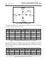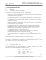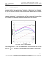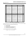
1
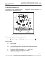
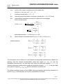
VERTEX ANTENNENTECHNIK GMBH
Doc.No.
Version:
OM1002114-21320
1.3
Table of Contents
1.
Introduction ................................................................................................................. 1
1.1
Purpose of this Manual ........................................................................................... 1
1.2
Software Identification............................................................................................. 1
1.3
Acronym List ........................................................................................................... 1
2.
Hexapod Kinematics ................................................................................................... 2
3.
Pointing Error Model ................................................................................................... 6
3.1
Overview................................................................................................................. 6
3.1.1
3.1.2
3.2
Corrections on Jack Level....................................................................................... 7
3.2.1
3.2.2
3.2.3
3.2.4
3.2.5
3.3
Components of Pointing Error Model ...........................................................................................6
Combination of Error Terms .........................................................................................................6
Overview .......................................................................................................................................7
Jackscrew pitch error....................................................................................................................8
Temperature Compensation .......................................................................................................11
Jackscrew Rotation Error............................................................................................................12
Support Cone Compensation Mode ...........................................................................................13
Corrections on Telescope Level............................................................................ 14
3.3.1
3.3.2
3.3.3
3.3.4
3.3.5
Overview .....................................................................................................................................14
Telescope Error Model ...............................................................................................................14
RF Refraction Correction ............................................................................................................18
Misalignment of Optical Telescope.............................................................................................19
Optical Refraction Model ............................................................................................................20
page ii
NOTE: THIS DOCUMENT CONTAINS PROPRIETARY INFORMATION AND MAY NOT BE DISCLOSED WITHOUT THE WRITTEN
CONSENT OF VERTEX ANTENNENTECHNIK GmbH, DUISBURG
VERTEX ANTENNENTECHNIK GMBH
Doc.No.
Version:
OM1002114-21320
1.3
VERTEX ANTENNENTECHNIK GmbH CONFIDENTIAL AND PROPRIETARY
All computer software, technical data or other information pertaining to the equipment covered by this
document is considered proprietary by VERTEX ANTENNENTECHNIK GmbH.
Such information transmitted in this document or related documents is for the benefit of
VERTEX ANTENNENTECHNIK GmbH customers and is not to be disclosed to other parties verbally
or in writing without prior written approval of VERTEX ANTENNENTECHNIK GmbH.
Additionally, this document may not be reproduced in whole or in part without written consent from
VERTEX ANTENNENTECHNIK GmbH.
Update Record
Release 1.2, Sep 2005
page 5:
handling of mount rotation changed
handling of u-joint coordinates added
Release 1.3, May 2006
par. 3.1.2:
par. 3.3.2:
par. 3.3.3:
par. 3.3.4:
par. 3.3.5:
description of error application in ACU modified
sign definition added
formula for calculation of water vapour pressure added
modified formula for OPT correction
new paragraph “optical refraction correction”
page iii
NOTE: THIS DOCUMENT CONTAINS PROPRIETARY INFORMATION AND MAY NOT BE DISCLOSED WITHOUT THE WRITTEN
CONSENT OF VERTEX ANTENNENTECHNIK GmbH, DUISBURG
VERTEX ANTENNENTECHNIK GMBH
Doc.No.
Version:
OM1002114-21320
1.3
1. INTRODUCTION
1.1
Purpose of this Manual
This section of the Servo System User Manual contains a description of the pointing error
model of the AMiBA Hexapod Telescope at Mauna Loa, Hawaii.
The pointing error model is used to eliminate known systematic pointing errors caused by
non-linearities, deformations, temperature variations etc. A description of the hexapod
kinematics is contained as well.
The compensation algorithms themselves are implemented in the Pointing Computer
(PTC). Any accessible parameters can be modified at the PTC, see part 3 of this User
Manual (description of PTC Local User Interface).
1.2
Software Identification
This Error Model Description describes the algorithms as implemented in the PTC
software version:
M1002114P-2.7.
1.3
ACU
Az
El
EMI
HPC
ICD
LCP
LUI
PCU
PLC
PTC
STC
Acronym List
Antenna Control Unit
Azimuth
Elevation
electromagnetic interference
Hexapod Computer
Interface Control Document
Local Control Panel
Local User Interface
Portable Control Unit
Programmable Logic Controller
Pointing Computer
Station Computer
page 1
NOTE: THIS DOCUMENT CONTAINS PROPRIETARY INFORMATION AND MAY NOT BE DISCLOSED WITHOUT THE WRITTEN
CONSENT OF VERTEX ANTENNENTECHNIK GmbH, DUISBURG
VERTEX ANTENNENTECHNIK GMBH
Doc.No.
Version:
OM1002114-21320
1.3
2. HEXAPOD KINEMATICS
The kinematics of the AMiBA telescope is a mathematical optimized kinematics of a
hexapod structure which is shown in Fig. 1.
s
Platform
Center of Gravity
4
5
6
Upper
Universal Joints
3
a
R1
1
α1o
2
Jackscrew
1
Y’
D
h
6
X’
3
4
2
5
Z
5
4
3
α1u
6
R2
Y
2
1
Lower
Universal Joints
X
Fig. 1: Hexapod coordinate system and mount parameters
The kinematical equation of the hexapod structure is
Li =
(Rz(ϕ
az
)
) Rx(ϕ zen ) Rz(ϕ pol ) Rz(ϕ az )T (mov i − v ) + v + dv − fix i , i = 1,...,6
with the notations
ϕaz
azimuth angle
ϕzen
zenith angle (ϕzen = π/2 - ϕel with elevation angle ϕel)
ϕpol
hexa-pol polarisation angle (alternatively obs-pol polarisation angle
ϕpol_Obs = ϕpol - ϕaz)
v
vector of the rotation point D with v = (0, 0, 3580)T [mm]
fix
vector of the (lower) fixed point of the jackscrew
with fixi = (xfi, yfi, zfi)T, i = 1,...,6
page 2
NOTE: THIS DOCUMENT CONTAINS PROPRIETARY INFORMATION AND MAY NOT BE DISCLOSED WITHOUT THE WRITTEN
CONSENT OF VERTEX ANTENNENTECHNIK GmbH, DUISBURG
VERTEX ANTENNENTECHNIK GMBH
Doc.No.
Version:
OM1002114-21320
1.3
mov
vector of the (upper) movable point of the jackscrew
with movi = (xmi, ymi, zmi)T, i = 1,...,6
L
Jackscrew length with Li, i = 1,...,6
dv1
manually pre-set translation movement (normally dv1 = (0, 0, 0)T [mm])
dv2
automatically translation movement to reduce the travel ranges
of the universal joints
⎛ sin(ϕ az ) ⎞
⎟
90° − ϕ el [°] ⎜
dv 2(ϕ az ,ϕ zen ) = a
⎜ − cos(ϕ az ) ⎟
90° − ϕ el ,min [°] ⎜
⎟
0
⎝
⎠
⎛ sin(ϕ az ) ⎞
⎟
ϕ zen ⎜
= a
⎜ − cos(ϕ az ) ⎟
θ max ⎜
⎟
⎝
0
⎠
optimized parameter : a = 850 mm, θmax = 60°
dv
total translation movement with dv(ϕaz,ϕzen) = dv1 + dv2(ϕaz,ϕzen)
rotation matrices
0
0 ⎞
⎛1
⎜
⎟
Rx(α ) := ⎜ 0 cos(α ) − sin(α ) ⎟
⎜ 0 sin(α ) cos(α ) ⎟
⎝
⎠
⎛ cos(α ) 0 sin(α ) ⎞
⎜
⎟
0
1
0) ⎟
Ry (α ) := ⎜
⎜ − sin(α ) 0 cos(α ) ⎟
⎝
⎠
⎛ cos(α ) − sin(α ) 0 ⎞
⎜
⎟
Rz(α ) := ⎜ sin(α ) cos(α ) 0 ⎟
⎜ 0
0
1⎟⎠
⎝
The kinematics can be different in the forward and backward transformation. Beside the
topology data the forward transformation needs the angles ϕaz, ϕzen, ϕpol and the
translation movement dv1 as input data and yields the jackscrew lengths Li, i = 1,...,6,
while the backward transformation needs the jackscrew lengths Li, i = 1,...,6 as input data
and yields the angles ϕaz, ϕzen, ϕpol and the translation movement dv1.
The global coordinate system of the AMiBA telescope together with the sky orientation is
shown in Fig. 2, assuming that the mount is orientated to due North.
page 3
NOTE: THIS DOCUMENT CONTAINS PROPRIETARY INFORMATION AND MAY NOT BE DISCLOSED WITHOUT THE WRITTEN
CONSENT OF VERTEX ANTENNENTECHNIK GmbH, DUISBURG
VERTEX ANTENNENTECHNIK GMBH
Doc.No.
Version:
OM1002114-21320
1.3
Fig. 2: Orientation of Hexapod Mount
The theoretical coordinates of the jackscrew points, which are given by an mathematical
optimization calculation, are listed in Table 1.
lower universal joints (variable “fix”)
upper universal joints (variable “mov”)
Jack
x [mm]
y [mm]
z [mm]
x [mm]
y [mm]
z [mm]
1
R2*cos(350°)
R2*sin(350°)
0.0
R1*cos(21°)
R1*sin(21°)
4620.0
2
R2*cos(70°)
R2*sin(70°)
0.0
R1*cos(39°)
R1*sin(39°)
4620.0
3
R2*cos(110°)
R2*sin(110°)
0.0
R1*cos(141°)
R1*sin(141°)
4620.0
4
R2*cos(190°)
R2*sin(190°)
0.0
R1*cos(159°)
R1*sin(159°)
4620.0
5
R2*cos(230°)
R2*sin(230°)
0.0
R1*cos(261°)
R1*sin(261°)
4620.0
6
R2*cos(310°)
R2*sin(310°)
0.0
R1*cos(279°)
R1*sin(279°)
4620.0
Table 1 : Theoretical jackscrew points with R1=1550.0, R2=1850.0
The real coordinates of the jackscrew points have been measured during in-plant
installation of the telescope in may 2004 in Duisburg, Germany by VERTEX. As a result of
fabrication tolerances the actual coordinates differ slightly from the theoretical ones. They
are listed in Table 2.
lower universal joints (variable “fix”)
upper universal joints (variable “mov”)
Jack
x [mm]
y [mm]
z [mm]
x [mm]
y [mm]
z [mm]
1
1822.8350
-320.5483
0.0
R1*cos(21°)
R1*sin(21°)
4620.0
2
632.4422
1738.0707
0.0
R1*cos(39°)
R1*sin(39°)
4620.0
3
-633.0782
1737.6624
0.0
R1*cos(141°)
R1*sin(141°)
4620.0
page 4
NOTE: THIS DOCUMENT CONTAINS PROPRIETARY INFORMATION AND MAY NOT BE DISCLOSED WITHOUT THE WRITTEN
CONSENT OF VERTEX ANTENNENTECHNIK GmbH, DUISBURG
VERTEX ANTENNENTECHNIK GMBH
Doc.No.
Version:
OM1002114-21320
1.3
lower universal joints (variable “fix”)
upper universal joints (variable “mov”)
Jack
x [mm]
y [mm]
z [mm]
x [mm]
y [mm]
z [mm]
4
-1823.6568
-320.3860
0.0
R1*cos(159°)
R1*sin(159°)
4620.0
5
-1191.2478
-1416.5320
0.0
R1*cos(261°)
R1*sin(261°)
4620.0
6
1190.9897
-1417.3090
0.0
R1*cos(279°)
R1*sin(279°)
4620.0
Table 2: Actual coordinates of the jackscrew points with R1=1550.0
The mount installation on Mauna Loa differs from this symmetrical coordinates; the Az = 0
axes of the telescope as shown in Fig. 1 does not point exactly to North but is rotated by
several degrees.
This Azimuth offset is must be entered at ACU, HPC and PTC as a parameter.
The following relationship applies:
Azsky = Azmount + OffsetAz
Internally, the coordinate transformations inside the three servo computer continue to use
the telescope coordinate system. Commands from user or superior computer was well as
position displays show the azimuth related to the “world coordinates”. The position
commands are converted accordingly before being entered into the hexapod coordinate
transformation:
Azmount,cmd = Azsky,cmd - OffsetAz
From this point of view, all azimuth angles contained in definitions and formulae earlier in
this paragraph are mount related azimuth angles.
The [mount related] coordinates of upper and lower u-joints are stored in an ASCII file on
the CF memory cards of ACU, PTC and HPC.
The coordinate files of all three computers must be identical at all times!
WARNING
Any significant change in coordinates, any typos or swapped digits may
lead to severe damage of the telescope because collision situations could
occur without being detected by software or hardware. Utmost caution is
needed when modifications to the geometry file(s) are required. Such
changes should only be modified by well trained and experienced staff.
The manufacturer cannot be held responsible for malfunctions and/or any
damage resulting from modification of the geometry file(s).
page 5
NOTE: THIS DOCUMENT CONTAINS PROPRIETARY INFORMATION AND MAY NOT BE DISCLOSED WITHOUT THE WRITTEN
CONSENT OF VERTEX ANTENNENTECHNIK GmbH, DUISBURG
VERTEX ANTENNENTECHNIK GMBH
Doc.No.
Version:
OM1002114-21320
1.3
3. POINTING ERROR MODEL
3.1
Overview
3.1.1
Components of Pointing Error Model
The pointing error model includes the following compensations:
- Compensation curves for jackscrew pitch non-linearities, based on i-plant calibration
measurements for each jacks (∆Lp).
- A compensation algorithm for jackscrew length variations due to temperature (∆Lt).
- A compensation for non-measured length variations of a jackscrew due to rotation of
the upper u-joints (∆Lr).
- An algorithm calculating the shift of the lower u-joint coordinates due to distortion of
the telescope base due to temperature.
- A compensation algorithm for deformations of the telescope including platform
depending on the actual position. This compensation is derived from error tables
generated during pointing calibration measurements (∆Azerr , ∆Elerr , ∆Polerr).
- A compensation algorithm for RF refraction (∆Elrefract)
- A compensation algorithm for optical refraction (required only for alignment
measurements using an optical pointing telescope) (∆Elrefract).
- A compensation algorithm for misalignment of the optical pointing telescope (∆Azopt ,
∆Elopt)
The actual corrections are displayed at the PTC Local User Interface.
The individual compensations can be enabled and disabled separately at the PTC Local
User Interface or from remote by the station computer.
3.1.2
Combination of Error Terms
The Pointing Computer will transfer the sum of all enabled corrections to the ACU,
separately for jack related and telescope level corrections.
∆Ltot,i
∆Aztot
∆Eltot
∆Poltot
=
=
=
=
∆Lp,i + ∆Lt,i + ∆Lr,i
∆Azerr + ∆Azopt
∆Elerr + ∆Elopt + ∆Elrefract
∆Polerr
page 6
NOTE: THIS DOCUMENT CONTAINS PROPRIETARY INFORMATION AND MAY NOT BE DISCLOSED WITHOUT THE WRITTEN
CONSENT OF VERTEX ANTENNENTECHNIK GmbH, DUISBURG
VERTEX ANTENNENTECHNIK GMBH
Doc.No.
Version:
OM1002114-21320
1.3
The ACU will apply the corrections as follows:
a) Actual jack length (Lact):
Lact = Lmeas,i + ∆Ltot,i
b) Commanded hexapod position:
Azcmd_forTransformation = Azcmd_nominal - ∆Aztot
Elcmd_forTransformation = Elcmd_nominal - ∆Eltot
Polcmd_forTransformation = Polcmd_nominal - ∆Poltot
c) Actual hexapod position:
Aztrue
Eltrue
Poltrue
= Azfrom_transformation + ∆Aztot
= Elfrom_transformation + ∆Eltot
= Polfrom_transformation + ∆Poltot
This actual position is displayed at the ACU and reported as actual position to the
STC. This means that the actual position always is the real position after applying all
corrections and not the uncorrected mount position.
3.2
Corrections on Jack Level
3.2.1
Overview
The corrections on jack level consist of the compensations for
- jackscrew pitch error,
- temperature compensation,
- jack length measuring error depending on telescope position
(due to rotation of upper u-joints)
- support cone deformation due to temperature.
All this corrections (except support cone correction) yield jack length corrections ∆L1 …
∆L6 for each of the jackscrews 1…6. On the other hand the special case effects a
coordinate change of the lower universal joints which also can be interpreted as a length
change of the jackscrews. All modules are described in the following chapters.
page 7
NOTE: THIS DOCUMENT CONTAINS PROPRIETARY INFORMATION AND MAY NOT BE DISCLOSED WITHOUT THE WRITTEN
CONSENT OF VERTEX ANTENNENTECHNIK GmbH, DUISBURG
VERTEX ANTENNENTECHNIK GMBH
Doc.No.
Version:
3.2.2
OM1002114-21320
1.3
Jackscrew pitch error
The telescope positioned is determined by measuring the positions of the six jackscrew
actuators. Since not the real length of the jackscrews is measured but only the rotation,
any jack pitch error (e.g. machining errors, non-linearities etc.) directly leads to a telescope
positioning error.
In order to be able to compensate for this error each jackscrew has undergone an in-plant
calibration measurement. A correlation function (see Fig. 3) between the linear movement
of the jackscrew and the encoder readout has been derived for each jackscrew.
Fig. 3: Error curves for jackscrew pitch
Each measurement curve in Fig. 3 can be described by a polynomial of the order 10 in the
10
form f ( x ) = ∑ ai x i . The vector a of the coefficients for each jackscrew is listed in Table 3.
i =0
page 8
NOTE: THIS DOCUMENT CONTAINS PROPRIETARY INFORMATION AND MAY NOT BE DISCLOSED WITHOUT THE WRITTEN
CONSENT OF VERTEX ANTENNENTECHNIK GmbH, DUISBURG
VERTEX ANTENNENTECHNIK GMBH
Doc.No.
Version:
OM1002114-21320
1.3
a
jackscrew 1
a0
jackscrew 2
-2.024509761765160*10
a1
-4.690421834325520*10
a2
a3
a4
1
-2
3.175818812949300*10
-3
1.000966699300860*10
-5
1.541352099930610*10
-8
jackscrew 3
4.254599813289640*10
2
-2.015506873855310*10
-2
-1.279223138765940*10
-4
-2.079059533885010*10
-6
-6.590341383524090*10
-9
a
1
a0
-1
a1
5.333730182112170*10
-4
a2
1.767559120263330*10
-6
a3
2.504907224531590*10
-9
a4
a5
-1.424616467483780*10
-3.014122368016800*10
1.387921160762620*10
-11
-9.238622036561910*10
-12
2.285806763018910*10
-12
a6
7.764892416501680*10
-15
-7.095505201937470*10
-15
1.446531162237440*10
-15
a6
a7
2.743812116375030*10
-18
-3.198287869016120*10
-18
6.245759670530750*10
-19
a7
5.973058848219020*10
-22
-8.457849525584240*10
-22
1.714087876766300*10
-22
a8
7.325619589449050*10
-26
-1.217131472371950*10
-25
2.645713864558710*10
-26
a9
3.877049825835910*10
-30
-7.368087558944830*10
-30
1.731246066850530*10
-30
a10
a5
a8
a9
a10
a
jackscrew 4
a0
jackscrew 5
2.743324175636780*10
a1
a2
a3
a4
1
1.816390007961940*10
-2
2.040482864105740*10
-3
6.306703070241420*10
-6
9.461016317632950*10
-9
8.105379713701580*10
-12
4.193397675987190*10
-15
a7
1.320217138374700*10
-18
a8
2.423328419428810*10
-22
2.285716445585560*10
-26
7.708311059986410*10
-31
a5
a6
a9
a10
jackscrew 6
-9.120596249290690*10
0
2.994017883033060*10
-2
1.853475595088450*10
-3
4.707048964999170*10
-6
5.301560895763430*10
-9
2.787891685747700*10
-12
3.403289908214870*10
-16
a
-2
a0
1.399391192743870*10
-1
a1
1.296102525136170*10
-3
a2
5.695909876093460*10
-6
a3
1.109389698870550*10
-8
a4
1.187703984708340*10
-11
a5
a6
-8.464647627231470*10
7.580116027803620*10
-15
-3.342955508378500*10
-19
2.961352291320270*10
-18
a7
-1.739067723782910*10
-22
6.948301798710590*10
-22
a8
-3.372908043046730*10
-26
8.991790206208470*10
-26
a9
-2.432377395612230*10
-30
4.932382220905220*10
-30
a10
Table 3: Vector ‘a’ for each jackscrew
Finally the measurement curves must shifted depending on of the real jackscrew length L
[mm] and the characteristic measurement data (see Fig. 4)
C1
C2
C3
C4
C5
jackscrew length,
reference switch,
measurement limit extended jackscrew,
measurement retracted jackscrew,
movement of the curve with C5 = -f(C2),
so that the jackscrew pitch error can be calculated by
∆L [mm] = (f (L − C1 + C 2) + C 5 ) 10 −3 .
page 9
NOTE: THIS DOCUMENT CONTAINS PROPRIETARY INFORMATION AND MAY NOT BE DISCLOSED WITHOUT THE WRITTEN
CONSENT OF VERTEX ANTENNENTECHNIK GmbH, DUISBURG
VERTEX ANTENNENTECHNIK GMBH
Doc.No.
Version:
OM1002114-21320
1.3
jackscrew pitch
0
0
C4
C2
C3
x
Measurement curve
Fig. 4: Jackscrew with measurement curve
The measurement curve is situated in the range of C4 < L-C1+C2 < C3. The data C1…C5
are listed in Table 4.
Jack
C1 [mm]
C2 [mm]
C3 [mm]
C4 [mm]
C5 [µm]
1
6150.366
-36.624
-19.1972
-3359.1970
14.7324
2
6149.009
-86.603
-47.7033
-3407.7029
-427.2679
3
6149.542
-38.486
-19.7907
-3359.79012
1.9514
4
6149.961
-25.151
-27.3491
-3367.3489
-28.1705
5
6150.103
-56.476
-35.8999
-3375.8999
5.6953
6
6150.360
-20.820
-17.6202
-3357.6202
2.4857
Table 4 : Correction factors for each jackscrew
The coefficient vector ‘a’ is coded in the hexapod software and the correction variables C1
until C5 are stored in an external file. This file has to be replaced along with the related
jackscrew if a jackscrew needs to be exchanged.
The correction algorithm yields length corrections ∆Lp1 until ∆Lp6.
page 10
NOTE: THIS DOCUMENT CONTAINS PROPRIETARY INFORMATION AND MAY NOT BE DISCLOSED WITHOUT THE WRITTEN
CONSENT OF VERTEX ANTENNENTECHNIK GmbH, DUISBURG
VERTEX ANTENNENTECHNIK GMBH
Doc.No.
Version:
3.2.3
OM1002114-21320
1.3
Temperature Compensation
The varying temperature of the different jackscrews with the length L produces a length
change ∆Lt of each jackscrew compared to the length at calibration temperature. Taking
into account the material specific thermal expansion coefficient α = 12.0 * 10-6 [1/K] and
the temperature difference ∆T between the individual jackscrews, which will be measured
and averaged by three temperature sensors (Psens1, ∆T1), (Psens2, ∆T2), (Psens3, ∆T3) along
the jackscrew (see Fig. 5),
L
jackscrew
Psens1
Psens2
Psens3
Fig. 5: Jackscrew with temperature sensors
the length change results approximately in a linear temperature characteristics function
⎧
⎪
⎪
⎪
⎪⎪
f ( x) = ⎨
⎪
⎪
⎪
⎪
⎪⎩
to
∆Lt =
∆T 1
x ≤ Psens1
∆T 1 Psens 2 − ∆T 2 Psens1
∆T 2 − ∆T 1
x +
Psens 2 − Psens1
Psens 2 − Psens1
∆T 2 Psens 3 − ∆T 3 Psens 2
∆T 3 − ∆T 2
x +
Psens 3 − Psens 2
Psens 3 − Psens 2
Psens1 < x ≤ Psens 2
if
x > Psens 3
∆T 3
Psens 1
∫α
Psens 2 < x ≤ Psens 3
f ( x) dx +
0
Psens 2
∫α
Psens 1
f ( x) dx +
Psens 3
∫α
f ( x) dx .
Psens 2
Calibration temperature is +17°C, so
∆T = Tsens – 17°C.
With the position of the sensors Psens1=122.0 mm, Psens2=1250.0 mm, Psens3=Li and
the readouts of the temperatures at the sensors, the results of the module temperature
correction are the correction lengths ∆Lt1 … ∆Lt6.
page 11
NOTE: THIS DOCUMENT CONTAINS PROPRIETARY INFORMATION AND MAY NOT BE DISCLOSED WITHOUT THE WRITTEN
CONSENT OF VERTEX ANTENNENTECHNIK GmbH, DUISBURG
VERTEX ANTENNENTECHNIK GMBH
Doc.No.
Version:
3.2.4
OM1002114-21320
1.3
Jackscrew Rotation Error
Each jackscrew spindle rotates with the angle βz (see also Fig. 6) relative to the jackscrew
nut when tilting and rotating the telescope mount. Because of the spindle thread a
jackscrew length change can occur which is not detected by the encoder on the still
standing worm gear shaft. This influence is calculated by a mathematical algorithm derived
from the kinematics of the jackscrew at any position.
ß
ßmx my
z''
movable point
y''
x''
jackscrew
ßz
z'
y'
fix point
ßfx ß
fy
x'
Fig. 6: Rotation of the jackscrew
Each jackscrew kinematics consists of the five degrees of rotations βfx, βfy, βmx, βmy and βz.
A special algorithm calculates the essential data βz. With a jackscrew pitch of p = 20
mm/rotation and the basis rotation angle βz,basis (is equal to βz in the hexapod basis
position) the jackscrew length error by rotation of the jackscrew against the fixed nut is
p
.
∆Lr = (β z ,basis − β z )
2 π
The algorithm is coded in the hexapod software and the results are the correction lengths
∆Lr1 … ∆Lr6.
page 12
NOTE: THIS DOCUMENT CONTAINS PROPRIETARY INFORMATION AND MAY NOT BE DISCLOSED WITHOUT THE WRITTEN
CONSENT OF VERTEX ANTENNENTECHNIK GmbH, DUISBURG
VERTEX ANTENNENTECHNIK GMBH
Doc.No.
Version:
OM1002114-21320
1.3
3.2.5
Support Cone Compensation Mode
The coordinates of the 6 lower (fixed) universal joints has been measured during in-plant
assembly of the AMiBA Telescope in May 2004 at an ambient temperature of 17° C. The x
and y coordinates vary with the temperature of the support cone. This error is taken into
account by the formulae
xnew = x * α * (T - T0)
ynew = y * α * (T - T0)
with the notations
α
specific thermal expansion coefficient with α = 12.0 * 10-6 [1/K],
T
average value of the temperature which is measured by several
sensors at the cone,
T0
basis measurement temperature of 17° C,
x, y coordinates of the lower (fixed) universal joints (see Table 2, page 5).
Together with the readout temperatures at the sensors and the original x, y coordinates of
the lower universal joints at a temperature of 17° C, the results of the module support cone
compensation mode are corrected x, y coordinates for the 6 lower universal joints.
page 13
NOTE: THIS DOCUMENT CONTAINS PROPRIETARY INFORMATION AND MAY NOT BE DISCLOSED WITHOUT THE WRITTEN
CONSENT OF VERTEX ANTENNENTECHNIK GmbH, DUISBURG
VERTEX ANTENNENTECHNIK GMBH
Doc.No.
Version:
OM1002114-21320
1.3
3.3
Corrections on Telescope Level
3.3.1
Overview
The corrections on telescope level consist of the compensations for
- error model for telescope and platform deformations,
- compensation algorithm for RF refraction
- compensation algorithm for optical refraction.
All this corrections (except support cone correction) yield position corrections ∆ϕaz, ∆ϕel
and ∆ϕpol.
3.3.2
Telescope Error Model
The idea of the telescope correction mode is to measure the telescope position errors
∆ϕaz, ∆ϕel and ∆ϕpol at different points on the sky by astronomical observation of well
known targets. All measurement points together make up a measurement grid. For
positions between the data points the delta positions can be calculated by interpolation.
For each data point, the hexapod position (Az, El, Pol) and the measured pointing errors
(dAz, dEl, dPol) are entered into a file named inter_un.dat (see sample file in Table 5). The
measurements make up an irregular grid of one sector of the sky. For a good pointing
accuracy both the sector size and the number of measurements should be as large as
possible. In addition, the measurements should be made at different polarisations.
Definition of sign of pointing error:
- Nominal position of object:
(AzN | ElN | PolN)
- The object has been found at (position display at ACU / PTC): (AzF | ElF | PolF)
- Error to be entered into table
at position
measured pointing error
(AzN | ElN | PolN)
(AzF - AzN | ElF - ElN | PolF - PolN)
page 14
NOTE: THIS DOCUMENT CONTAINS PROPRIETARY INFORMATION AND MAY NOT BE DISCLOSED WITHOUT THE WRITTEN
CONSENT OF VERTEX ANTENNENTECHNIK GmbH, DUISBURG
VERTEX ANTENNENTECHNIK GMBH
Doc.No.
Version:
OM1002114-21320
1.3
Transform measurement data by an irregular grid to an regular grid
=================================================================
calculation for an regular grid
azimuth area [degree]
0.00
elevation area [degree]
30.00
polarisation area [degree]
-25.00
360.00
90.00
10.00
measurement data, irregular grid
Az
El
Pol
0.00000000
30.00000000
-30.00000000
20.00000000
30.00000000
-30.00000000
40.00000000
30.00000000
-30.00000000
60.00000000
30.00000000
-30.00000000
80.00000000
30.00000000
-30.00000000
160.00000000
30.00000000
-30.00000000
180.00000000
30.00000000
-30.00000000
200.00000000
30.00000000
-30.00000000
220.00000000
30.00000000
-30.00000000
100.00000000
30.00000000
-30.00000000
120.00000000
30.00000000
-30.00000000
140.00000000
30.00000000
-30.00000000
step
step
step
5.00
5.00
5.00
dAz
1.00000000
5.00000000
4.00000000
3.00000000
6.00000000
3.00000000
4.00000000
6.00000000
7.00000000
7.00000000
3.00000000
2.00000000
dEl
1.00000000
1.00000000
1.00000000
1.00000000
2.00000000
7.00000000
2.00000000
3.00000000
4.00000000
3.00000000
4.00000000
6.00000000
dPol
1.00000000
2.00000000
3.00000000
4.00000000
6.00000000
4.00000000
1.00000000
4.00000000
5.00000000
7.00000000
2.00000000
3.00000000
Table 5: Unsorted position measurements in file inter_un.dat
The actual position for Pol in the both irregular and regular grids must always be entered
as Hex-Pol (polarisation related to the hexapod mount).
After the measurements are done the irregular grid must be transformed into a regular grid
and the result is saved in a file named inter.dat (see sample in Table 6).
The file must contain the characteristic data of the regular grid in lines 2…4 as shown in
the sample file. This includes:
- upper and lower limits of measured sector in Az, El and Pol
- step size for regular grid in Az, El and Pol.
The grid steps may be different for Az, El and Pol. The interpolation algorithm does not
require a particular step size. However, the maximum number of lines in this file may not
exceed 100,000.
A possible mathematical algorithm to get a regular grid is known as Shepard method. It
can be used as stand-alone software. This method (and of course all other mathematical
methods) is only effective inside the measurement sector. Interpolations for positions
outside the measurement sector may be inaccurate.
Activating the telescope error model correction requires a file inter.dat. This must be saved
on the disk on the PTC flash card in the same directory as the executable software. To
read a new file inter.dat the PTC must be re-bootet.
page 15
NOTE: THIS DOCUMENT CONTAINS PROPRIETARY INFORMATION AND MAY NOT BE DISCLOSED WITHOUT THE WRITTEN
CONSENT OF VERTEX ANTENNENTECHNIK GmbH, DUISBURG
VERTEX ANTENNENTECHNIK GMBH
Doc.No.
Version:
OM1002114-21320
1.3
The correction software calculates by interpolation the position errors ∆ϕaz, ∆ϕel and ∆ϕpol
as a function of the present telescope position. Therefore the regular grid has a great
computer time advantage adverse the irregular grid. The linear interpolation algorithm
searches the cube of the neighbouring positions in the grid which encloses the actual
position, and interpolates the position errors assigned to each corner of the cube. The file
inter.dat must contain identical lines for Az = 0 deg and Az = 360 deg.
The telescope error model yields position corrections ∆Azerr, ∆Elerr and ∆Polerr.
page 16
NOTE: THIS DOCUMENT CONTAINS PROPRIETARY INFORMATION AND MAY NOT BE DISCLOSED WITHOUT THE WRITTEN
CONSENT OF VERTEX ANTENNENTECHNIK GmbH, DUISBURG
VERTEX ANTENNENTECHNIK GMBH
Doc.No.
Version:
OM1002114-21320
1.3
Calculation for an regular grid
azimuth area [degree]
0.0000
elevation area [degree]
30.0000
polarisation area [degree]
-25.0000
Az
0.00000000
0.00000000
0.00000000
0.00000000
0.00000000
0.00000000
0.00000000
0.00000000
0.00000000
0.00000000
0.00000000
0.00000000
0.00000000
0.00000000
0.00000000
0.00000000
0.00000000
0.00000000
El
30.00000000
30.00000000
30.00000000
30.00000000
30.00000000
30.00000000
30.00000000
30.00000000
35.00000000
35.00000000
35.00000000
35.00000000
35.00000000
35.00000000
35.00000000
35.00000000
40.00000000
40.00000000
360.0000
90.0000
10.0000
Pol
-25.00000000
-20.00000000
-15.00000000
-10.00000000
-5.00000000
0.00000000
5.00000000
10.00000000
-25.00000000
-20.00000000
-15.00000000
-10.00000000
-5.00000000
0.00000000
5.00000000
10.00000000
-25.00000000
-20.00000000
step
step
step
5.0000
5.0000
5.0000
dAz
0.06819019
0.06818528
0.06818039
0.06817552
0.06817067
0.06816586
0.06816108
0.06815635
0.06829306
0.06828835
0.06828363
0.06827888
0.06827412
0.06826935
0.06826458
0.06825981
0.06839662
0.06839212
dEl
-0.00858209
-0.00858367
-0.00858527
-0.00858688
-0.00858849
-0.00859011
-0.00859174
-0.00859336
-0.00857819
-0.00857977
-0.00858136
-0.00858296
-0.00858458
-0.00858620
-0.00858782
-0.00858946
-0.00857429
-0.00857586
dPol
0.00000000
0.00000000
0.00000000
0.00000000
0.00000000
0.00000000
0.00000000
0.00000000
0.00000000
0.00000000
0.00000000
0.00000000
0.00000000
0.00000000
0.00000000
0.00000000
0.00000000
0.00000000
..................................................................
..................................................................
..................................................................
360.00000000
360.00000000
360.00000000
360.00000000
360.00000000
360.00000000
360.00000000
360.00000000
360.00000000
360.00000000
360.00000000
360.00000000
360.00000000
360.00000000
360.00000000
360.00000000
85.00000000
85.00000000
85.00000000
85.00000000
85.00000000
85.00000000
85.00000000
85.00000000
90.00000000
90.00000000
90.00000000
90.00000000
90.00000000
90.00000000
90.00000000
90.00000000
-25.00000000
-20.00000000
-15.00000000
-10.00000000
-5.00000000
0.00000000
5.00000000
10.00000000
-25.00000000
-20.00000000
-15.00000000
-10.00000000
-5.00000000
0.00000000
5.00000000
10.00000000
0.11690180
0.13483681
0.16171136
0.20329068
0.28139628
0.37440990
0.28172032
0.20456258
0.12713996
0.14697311
0.17562134
0.21738251
0.27689824
0.31867511
0.27740887
0.21882686
-0.00683586
-0.00670948
-0.00655411
-0.00648106
-0.00676227
-0.00703623
-0.00677584
-0.00656923
-0.00680790
-0.00664064
-0.00644921
-0.00631872
-0.00643678
-0.00665926
-0.00645507
-0.00639312
0.00000000
0.00000000
0.00000000
0.00000000
0.00000000
0.00000000
0.00000000
0.00000000
0.00000000
0.00000000
0.00000000
0.00000000
0.00000000
0.00000000
0.00000000
0.00000000
Table 6: Sample file inter.dat
page 17
NOTE: THIS DOCUMENT CONTAINS PROPRIETARY INFORMATION AND MAY NOT BE DISCLOSED WITHOUT THE WRITTEN
CONSENT OF VERTEX ANTENNENTECHNIK GmbH, DUISBURG
VERTEX ANTENNENTECHNIK GMBH
Doc.No.
Version:
OM1002114-21320
1.3
3.3.3
RF Refraction Correction
The PTC also compensates for atmospheric radio refraction1. Enabling/disabling is
possible at the PTC Local User Interface.
The algorithm used is taken from 'Astrophysical Quantities', by C.W. Allen (3rd edition,
page 124), and is :
N
ref0
∆Elrefract
= 1 - (7.8e-5 * P + 0.39 * e/T)/T
= (N*N - 1)/2*N*N
= ref0/tan(alt)
where
P
e
T
alt
atmospheric pressure in mb (hPa)
water vapour pressure in mb (hPa)
temperature in Kelvin
altitude
The correction ∆Elrefract is to be added to the true altitude to give the apparent altitude.
Actual weather data can be transferred by the station computer to the PTC in order to
keep the compensation as accurate as possible.
Calculation of water vapour pressure (e) from relative humidity:
e
=
RH/100 * ES
ES
=
c0 * 10**[ c1*Tc / (c2 + Tc) ]
where:
1
e
RH
ES
Tc
c0
c1
c2
=
=
=
=
=
=
=
water vapour pressure in mb (hPa)
relative humidity in %
saturation pressure of water vapour in mb (hPa)
temperature, deg C
6.1078
7.5
237.3
Algorithms provided by ASIAA
page 18
NOTE: THIS DOCUMENT CONTAINS PROPRIETARY INFORMATION AND MAY NOT BE DISCLOSED WITHOUT THE WRITTEN
CONSENT OF VERTEX ANTENNENTECHNIK GmbH, DUISBURG
VERTEX ANTENNENTECHNIK GMBH
Doc.No.
Version:
3.3.4
OM1002114-21320
1.3
Misalignment of Optical Telescope
This correction is only required during observations with the optical pointing telescope. It
compensates for any misalignments of this device compared to the pointing direction of
the main telescope.
The (x,y,z)-right hand frame of an optical telescope is positioned on the AMiBA platform,
whereas the z-axis is normal to the platform and the y-axis the reference line for ϕpol = 0
degree. With the notations
Hx
angle in the x-z plane (rotation around the y-axis, for small angles it points
along the x-axis)
Hy
angle in the y-z-plane
the pointing correction angles are2
∆Az opt =
Hx cos(ϕ az + ϕ pol ) + Hy sin(ϕ az + ϕ pol )
cos(ϕ el )
∆El opt = Hy cos(ϕ az + ϕ pol ) − Hx sin(ϕ az + ϕ pol ) .
The parameters Hx and Hy can be entered at the PTC Local User Interface, see part 3 of
this manual.
The correction algorithm yields position corrections ∆Azopt and ∆Elopt. There is no error in
polarization.
2
Formula provided by ASIAA
page 19
NOTE: THIS DOCUMENT CONTAINS PROPRIETARY INFORMATION AND MAY NOT BE DISCLOSED WITHOUT THE WRITTEN
CONSENT OF VERTEX ANTENNENTECHNIK GmbH, DUISBURG
VERTEX ANTENNENTECHNIK GMBH
Doc.No.
Version:
3.3.5
OM1002114-21320
1.3
Optical Refraction Model
The optical refraction is required only for alignment measurements using an optical
pointing telescope. During normal operation this refraction should be disabled.
Enabling/disabling is only possible at the PTC Local User Interface.
Correction formula:
∆Φ Re frOPT = 1.2 *
TDK:
PMB:
ZD:
60.101 * tan( ZD ) − 0.0668 * tan 3 ( ZD ) PMB 283.15
*
*
(180 / pi ) * 3600
1013.2 TDK
Ambient temperature [K]
Atmospheric pressure [mbar]
Distance from zenith [rad] = (90 degr - ΦEl) * π/180
The formula yields REF in radians.
page 20
NOTE: THIS DOCUMENT CONTAINS PROPRIETARY INFORMATION AND MAY NOT BE DISCLOSED WITHOUT THE WRITTEN
CONSENT OF VERTEX ANTENNENTECHNIK GmbH, DUISBURG
VERTEX ANTENNENTECHNIK GMBH
Doc.No.
Version:
OM1002114-21320
1.3
This page intentionally left blank.
page 21
NOTE: THIS DOCUMENT CONTAINS PROPRIETARY INFORMATION AND MAY NOT BE DISCLOSED WITHOUT THE WRITTEN
CONSENT OF VERTEX ANTENNENTECHNIK GmbH, DUISBURG