Download Tulip User Manual

Tulip User Manual
Tulip User Manual
Table of Contents
1. Introduction . . . . . . . . . . . . . . . . . . . . . . . . . . . . . . . . . . . . . . . . . . . . . . . . . . . . . . . . . . . . . . . . . . . . . . . . . . . . . . . . 1
2. Graphic Interface . . . . . . . . . . . . . . . . . . . . . . . . . . . . . . . . . . . . . . . . . . . . . . . . . . . . . . . . . . . . . . . . . . . . . . . . . . . 2
2.1. Main window : Menus . . . . . . . . . . . . . . . . . . . . . . . . . . . . . . . . . . . . . . . . . . . . . . . . . . . . . . . . . . . . . . . 2
2.2. Main window : Tools bar . . . . . . . . . . . . . . . . . . . . . . . . . . . . . . . . . . . . . . . . . . . . . . . . . . . . . . . . . . . . . 4
2.3. Graph Editor . . . . . . . . . . . . . . . . . . . . . . . . . . . . . . . . . . . . . . . . . . . . . . . . . . . . . . . . . . . . . . . . . . . . . . . . 5
2.3.1. Property . . . . . . . . . . . . . . . . . . . . . . . . . . . . . . . . . . . . . . . . . . . . . . . . . . . . . . . . . . . . . . . . . . . . . 5
2.3.2. Element . . . . . . . . . . . . . . . . . . . . . . . . . . . . . . . . . . . . . . . . . . . . . . . . . . . . . . . . . . . . . . . . . . . . . 7
2.3.3. Hierarchy . . . . . . . . . . . . . . . . . . . . . . . . . . . . . . . . . . . . . . . . . . . . . . . . . . . . . . . . . . . . . . . . . . . . 7
2.3.4. Statistics (not available in standard version) . . . . . . . . . . . . . . . . . . . . . . . . . . . . . . . . . . . . . 8
2.4. View Editor . . . . . . . . . . . . . . . . . . . . . . . . . . . . . . . . . . . . . . . . . . . . . . . . . . . . . . . . . . . . . . . . . . . . . . . . 11
2.5. Standards views . . . . . . . . . . . . . . . . . . . . . . . . . . . . . . . . . . . . . . . . . . . . . . . . . . . . . . . . . . . . . . . . . . . . 11
2.5.1. Node Link Diagram view . . . . . . . . . . . . . . . . . . . . . . . . . . . . . . . . . . . . . . . . . . . . . . . . . . . . . 11
2.5.2. Parallel Coordinates view . . . . . . . . . . . . . . . . . . . . . . . . . . . . . . . . . . . . . . . . . . . . . . . . . . . . 18
2.5.3. Table view . . . . . . . . . . . . . . . . . . . . . . . . . . . . . . . . . . . . . . . . . . . . . . . . . . . . . . . . . . . . . . . . . . 29
3. Functionalities . . . . . . . . . . . . . . . . . . . . . . . . . . . . . . . . . . . . . . . . . . . . . . . . . . . . . . . . . . . . . . . . . . . . . . . . . . . . 31
3.1. Management of Graphs . . . . . . . . . . . . . . . . . . . . . . . . . . . . . . . . . . . . . . . . . . . . . . . . . . . . . . . . . . . . . 31
3.1.1. The “Find” tool . . . . . . . . . . . . . . . . . . . . . . . . . . . . . . . . . . . . . . . . . . . . . . . . . . . . . . . . . . . . . 32
3.2. Algorithms . . . . . . . . . . . . . . . . . . . . . . . . . . . . . . . . . . . . . . . . . . . . . . . . . . . . . . . . . . . . . . . . . . . . . . . . 32
3.2.1. Selection Algorithms . . . . . . . . . . . . . . . . . . . . . . . . . . . . . . . . . . . . . . . . . . . . . . . . . . . . . . . . 32
3.2.2. Color Algorithms : . . . . . . . . . . . . . . . . . . . . . . . . . . . . . . . . . . . . . . . . . . . . . . . . . . . . . . . . . . 38
3.2.3. Measure . . . . . . . . . . . . . . . . . . . . . . . . . . . . . . . . . . . . . . . . . . . . . . . . . . . . . . . . . . . . . . . . . . . . 41
3.2.4. Layout . . . . . . . . . . . . . . . . . . . . . . . . . . . . . . . . . . . . . . . . . . . . . . . . . . . . . . . . . . . . . . . . . . . . . 52
3.2.5. Size . . . . . . . . . . . . . . . . . . . . . . . . . . . . . . . . . . . . . . . . . . . . . . . . . . . . . . . . . . . . . . . . . . . . . . . . 60
3.2.6. General . . . . . . . . . . . . . . . . . . . . . . . . . . . . . . . . . . . . . . . . . . . . . . . . . . . . . . . . . . . . . . . . . . . . 61
3.3. Properties of graph . . . . . . . . . . . . . . . . . . . . . . . . . . . . . . . . . . . . . . . . . . . . . . . . . . . . . . . . . . . . . . . . . 62
3.3.1. Rendering Properties . . . . . . . . . . . . . . . . . . . . . . . . . . . . . . . . . . . . . . . . . . . . . . . . . . . . . . . . 62
3.3.2. Using Properties . . . . . . . . . . . . . . . . . . . . . . . . . . . . . . . . . . . . . . . . . . . . . . . . . . . . . . . . . . . . 63
3.4. Hierarchy . . . . . . . . . . . . . . . . . . . . . . . . . . . . . . . . . . . . . . . . . . . . . . . . . . . . . . . . . . . . . . . . . . . . . . . . . . 64
3.4.1. Definitions : . . . . . . . . . . . . . . . . . . . . . . . . . . . . . . . . . . . . . . . . . . . . . . . . . . . . . . . . . . . . . . . . 64
3.4.2. Creating subgraphs or Groups : . . . . . . . . . . . . . . . . . . . . . . . . . . . . . . . . . . . . . . . . . . . . . . . 66
3.4.3. Deleting / Ungrouping a subgraph or a Group : . . . . . . . . . . . . . . . . . . . . . . . . . . . . . . . . . 67
3.4.4. Using subgraphs or groups : . . . . . . . . . . . . . . . . . . . . . . . . . . . . . . . . . . . . . . . . . . . . . . . . . . 67
3.4.5. Algorithms that creates subgraphs : . . . . . . . . . . . . . . . . . . . . . . . . . . . . . . . . . . . . . . . . . . . 67
3.5. Statistics Panel (not available in standard version) . . . . . . . . . . . . . . . . . . . . . . . . . . . . . . . . . . . . . . 68
3.6. Text Rendering . . . . . . . . . . . . . . . . . . . . . . . . . . . . . . . . . . . . . . . . . . . . . . . . . . . . . . . . . . . . . . . . . . . . . 68
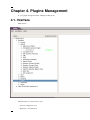
4. Plugins Management . . . . . . . . . . . . . . . . . . . . . . . . . . . . . . . . . . . . . . . . . . . . . . . . . . . . . . . . . . . . . . . . . . . . . . . 70
4.1. Interface . . . . . . . . . . . . . . . . . . . . . . . . . . . . . . . . . . . . . . . . . . . . . . . . . . . . . . . . . . . . . . . . . . . . . . . . . . . 70
4.1.1. Plugins List . . . . . . . . . . . . . . . . . . . . . . . . . . . . . . . . . . . . . . . . . . . . . . . . . . . . . . . . . . . . . . . . . 71
4.1.2. Plugin’s Documentation . . . . . . . . . . . . . . . . . . . . . . . . . . . . . . . . . . . . . . . . . . . . . . . . . . . . . . 71
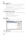
4.2. Setup . . . . . . . . . . . . . . . . . . . . . . . . . . . . . . . . . . . . . . . . . . . . . . . . . . . . . . . . . . . . . . . . . . . . . . . . . . . . . 71
4.2.1. Add a server . . . . . . . . . . . . . . . . . . . . . . . . . . . . . . . . . . . . . . . . . . . . . . . . . . . . . . . . . . . . . . . . 71
4.2.2. Modify/Remove a server . . . . . . . . . . . . . . . . . . . . . . . . . . . . . . . . . . . . . . . . . . . . . . . . . . . . . 72
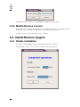
4.3. Install/Remove plugins . . . . . . . . . . . . . . . . . . . . . . . . . . . . . . . . . . . . . . . . . . . . . . . . . . . . . . . . . . . . . . 72
4.3.1. Simple installation . . . . . . . . . . . . . . . . . . . . . . . . . . . . . . . . . . . . . . . . . . . . . . . . . . . . . . . . . . . 72
4.3.2. Installation/Remove with dependencies . . . . . . . . . . . . . . . . . . . . . . . . . . . . . . . . . . . . . . . . 73
5. Tutorials . . . . . . . . . . . . . . . . . . . . . . . . . . . . . . . . . . . . . . . . . . . . . . . . . . . . . . . . . . . . . . . . . . . . . . . . . . . . . . . . . . 74
5.1. First Step . . . . . . . . . . . . . . . . . . . . . . . . . . . . . . . . . . . . . . . . . . . . . . . . . . . . . . . . . . . . . . . . . . . . . . . . . . 74
5.1.1. First graph display . . . . . . . . . . . . . . . . . . . . . . . . . . . . . . . . . . . . . . . . . . . . . . . . . . . . . . . . . . . 74
5.1.2. Save options . . . . . . . . . . . . . . . . . . . . . . . . . . . . . . . . . . . . . . . . . . . . . . . . . . . . . . . . . . . . . . . . 75
5.1.3. Algorithms . . . . . . . . . . . . . . . . . . . . . . . . . . . . . . . . . . . . . . . . . . . . . . . . . . . . . . . . . . . . . . . . . 75
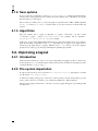
5.2. Improving a layout . . . . . . . . . . . . . . . . . . . . . . . . . . . . . . . . . . . . . . . . . . . . . . . . . . . . . . . . . . . . . . . . . 75
5.2.1. Introduction . . . . . . . . . . . . . . . . . . . . . . . . . . . . . . . . . . . . . . . . . . . . . . . . . . . . . . . . . . . . . . . . 75
5.2.2. File-system importation . . . . . . . . . . . . . . . . . . . . . . . . . . . . . . . . . . . . . . . . . . . . . . . . . . . . . . 75
5.2.3. Using other Layouts : . . . . . . . . . . . . . . . . . . . . . . . . . . . . . . . . . . . . . . . . . . . . . . . . . . . . . . . . 76
5.2.4. Showing Labels . . . . . . . . . . . . . . . . . . . . . . . . . . . . . . . . . . . . . . . . . . . . . . . . . . . . . . . . . . . . . 79
5.2.5. Showing a specific kind of file. . . . . . . . . . . . . . . . . . . . . . . . . . . . . . . . . . . . . . . . . . . . . . . . 81
iii
Tulip
User
Manual
5.2.6. Conclusion . . . . . . . . . . . . . . . . . . . . . . . . . . . . . . . . . . . . . . . . . . . . . . . . . . . . . . . . . . . . . . . . . 82
5.3. People in InfoVis . . . . . . . . . . . . . . . . . . . . . . . . . . . . . . . . . . . . . . . . . . . . . . . . . . . . . . . . . . . . . . . . . . . 82
5.3.1. Analyzing an author. . . . . . . . . . . . . . . . . . . . . . . . . . . . . . . . . . . . . . . . . . . . . . . . . . . . . . . . . 83
5.3.2. What, if any, are the relationships between two or more or all researchers . . . . . . . . . . 87
5.4. Statistics Panel (not available in the downloadable binary versions, requires configuration with
--enable-stats-gui when compiling Tulip from source code) . . . . . . . . . . . . . . . . . . . . . . . . . . . . . . . . . . 97
5.4.1. Introduction . . . . . . . . . . . . . . . . . . . . . . . . . . . . . . . . . . . . . . . . . . . . . . . . . . . . . . . . . . . . . . . . 97
5.4.2. Scatter plot and Histogram computation . . . . . . . . . . . . . . . . . . . . . . . . . . . . . . . . . . . . . . . . 98
5.4.3. Statistics values and Augmented displays . . . . . . . . . . . . . . . . . . . . . . . . . . . . . . . . . . . . . 102
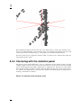
5.4.4. Clustering with the statistics panel . . . . . . . . . . . . . . . . . . . . . . . . . . . . . . . . . . . . . . . . . . . 105
5.4.5. Conclusion . . . . . . . . . . . . . . . . . . . . . . . . . . . . . . . . . . . . . . . . . . . . . . . . . . . . . . . . . . . . . . . . 108
iv
List of Figures
2.1. Computation Tab . . . . . . . . . . . . . . . . . . . . . . . . . . . . . . . . . . . . . . . . . . . . . . . . . . . . . . . . . . . . . . . . . . . . . . . . . . 8
2.2. Display Tab . . . . . . . . . . . . . . . . . . . . . . . . . . . . . . . . . . . . . . . . . . . . . . . . . . . . . . . . . . . . . . . . . . . . . . . . . . . . . . 9
2.3. ClusteringTab . . . . . . . . . . . . . . . . . . . . . . . . . . . . . . . . . . . . . . . . . . . . . . . . . . . . . . . . . . . . . . . . . . . . . . . . . . . 10
3.1. Bitmap Rendering . . . . . . . . . . . . . . . . . . . . . . . . . . . . . . . . . . . . . . . . . . . . . . . . . . . . . . . . . . . . . . . . . . . . . . . 68
3.2. 3D Rendering . . . . . . . . . . . . . . . . . . . . . . . . . . . . . . . . . . . . . . . . . . . . . . . . . . . . . . . . . . . . . . . . . . . . . . . . . . . 68
3.3. Texture Rendering . . . . . . . . . . . . . . . . . . . . . . . . . . . . . . . . . . . . . . . . . . . . . . . . . . . . . . . . . . . . . . . . . . . . . . . 69
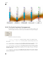
5.1. Statistics base test set : a tree . . . . . . . . . . . . . . . . . . . . . . . . . . . . . . . . . . . . . . . . . . . . . . . . . . . . . . . . . . . . . . 98
5.2. The metrics available in the statistics panel . . . . . . . . . . . . . . . . . . . . . . . . . . . . . . . . . . . . . . . . . . . . . . . . . 98
5.3. A single metric for an histogram . . . . . . . . . . . . . . . . . . . . . . . . . . . . . . . . . . . . . . . . . . . . . . . . . . . . . . . . . . . 99
5.4. Your first histogram . . . . . . . . . . . . . . . . . . . . . . . . . . . . . . . . . . . . . . . . . . . . . . . . . . . . . . . . . . . . . . . . . . . . . 100
5.5. Scatter plot generated from the three metrics . . . . . . . . . . . . . . . . . . . . . . . . . . . . . . . . . . . . . . . . . . . . . . . 101
5.6. Click on the button Compute Result to enable the tab . . . . . . . . . . . . . . . . . . . . . . . . . . . . . . . . . . . . . . . 102
5.7. Checking Average on the display tab . . . . . . . . . . . . . . . . . . . . . . . . . . . . . . . . . . . . . . . . . . . . . . . . . . . . . . 103
5.8. The average of the scatter plot . . . . . . . . . . . . . . . . . . . . . . . . . . . . . . . . . . . . . . . . . . . . . . . . . . . . . . . . . . . . 104
5.9. Selection of the clustering value . . . . . . . . . . . . . . . . . . . . . . . . . . . . . . . . . . . . . . . . . . . . . . . . . . . . . . . . . . 105
5.10. The clustering plane . . . . . . . . . . . . . . . . . . . . . . . . . . . . . . . . . . . . . . . . . . . . . . . . . . . . . . . . . . . . . . . . . . . 106
5.11. The new clusters after statistic clustering . . . . . . . . . . . . . . . . . . . . . . . . . . . . . . . . . . . . . . . . . . . . . . . . . 107
v
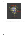
Chapter 1. Introduction
The research by the information visualization community show clearly that using a visual representation of data-sets enables faster analysis by the end users. Tulip, created by David AUBER, is a
contribution of the area of information visualization, “InfoViz”. Even if the Tulip framework enables
the visualization, the drawing and the edition of small graphs, all the parts of the framework have been
built in order to be able to visualize graphs having to 1.000.000 elements. A visualization system must
draw and display huge graphs, enables to navigate through geometric operations as well as extracts
subgraphs of the data and allows to change the representation of the results obtained by filtering.
1
Chapter 2. Graphic Interface
2.1. Main window : Menus
The main window of Tulip software is composed of several subwindows and a menu bar :
• File: this menu is used for usual file operations : New(Ctrl+N, APPLE+N on Mac),
Open(Ctrl+O, APPLE+0 on Mac), Save(Ctrl+S, APPLE+S on Mac), Save As(Ctrl+Shift+S, APPLE+Shift+S on Mac), Print(Ctrl+P, APPLE+P on Mac) and Exit(Ctrl+Q, APPLE+Q on Mac). Others
are added:
• Import: this submenu is populated by import plugins.
• File : Plugins allowing importation of graph files in different format such as Adjacent Matrix, gml,
dot (graphviz), or tlp (tulip default file format).
• Graph : Plugins allowing the creation of randomly generated graphs of different types.
• Misc : Plugins to capture the tree structure of a file system directory, or the graph structure of a web
site.
• Export: this submenu is populated by export plugins allowing to save a tulip graph accordingly to a
specified format. By default Tulip is able to export in GML and TLP formats.
• Edit: this is composed of tools : Cut(Ctrl+X, APPLE+X on Mac), Copy(Ctrl+C, APPLE+C on Mac), Paste(Ctrl+V, APPLE+V on Mac), and Find(Ctrl+F, APPLE+F on Mac), which affect the selected elements. This menu contains also: Select All(Ctrl+A, APPLE+A on Mac), Delete selection(Del), Deselect all(Ctrl+Shift+A, APPLE+Shift+A on Mac), Invert Selection(Ctrl+I, APPLE+I on
Mac), Create group(Ctrl+G, APPLE+G on Mac), Create subgraph(Ctrl+Shift+G, APPLE+Shift+G on
Mac), Undo(Ctrl+Z, APPLE+Z on Mac), Redo(Ctrl+Y, APPLE+Y on Mac).More details on the Find
tool : The find tool has 4 options :
• Replace : Replace the current selection (nodes or edges already selected).
• Add : Add the nodes (or edges) to be selected to the current selection.
• Remove : Remove nodes (or edges) from the current selection.
• Intersect : Select the intersection between the nodes (or edges) TO BE selected, and the ones from the
current selection.
• Algorithm: this one is divided in several parts to make a difference between the kind of
algorithms you can apply. These are:
• Selection: this submenu is populated by ’selection’ algorithms. These algorithms allows to select
nodes and or edges (assign the ’viewSelection’ property see Section 3.3, “Properties of graph” for more
details) satifying some criteria. For example the ’Loop Selection’ algorithm detects all edges for which the
starting and ending nodes are the same.
• Color: this submenu is populated by ’color’ algorithms. These king of algorithm computes the color
(the ’viewColor’ property see Section 3.3, “Properties of graph” for more details ) of the graph elements.
A default one, ’Metric Mapping’, is provided; it allows to color all graph elements according to a metric
property.
2
Graphic
Interface
• Measure: this submenu is populated by ’metric’ algorithms. These algorithms allows to compute and
assigned a value to the ’viewMetric’ property of graph elements see Section 3.3, “Properties of graph” for
more details. For example, when running the ’Degree’ algorithm, the degree (the number of its neighbors)
is compute and assigned to each graph node ’viewMetric’ property.
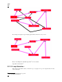
• Layout: this submenu is populated by ’layout’ algorithms which allow to display graphs using different
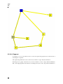
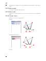
types of drawings. For example, the ’Circular’ algorithm places all nodes of a graph along a circle. Before
:
After :
• Size: this submenu is populated by ’size’ algorithms which allow to compute the size (the ’viewSize’
property see Section 3.3, “Properties of graph” for more details) of the graph elements.
• General: this submenu is populated by more general algorithms for computing properties, subgraphs,
quotient graphs, groups... For example the ’Equal Value’ algorithm create subgraphs for which the included
elements have the same value for a choosed ’metric’ property.
For more information please visit Section 3.2, “Algorithms”
• Graph : This menu is composed of 2 sub menus :
• Tests: This sub menu contains tools able to say if the graph obey some constraints :
• Simple : Is the Graph Simple ? For more information please visit : Wikipedia: Simple graphs1
• Directed Tree : A directed tree is a directed graph which would be a tree if the directions on
the edges were ignored. Some authors restrict the phrase to the case where the edges are all directed
towards a particular vertex, or all directed away from a particular vertex. For more information please
visit : Wikipedia: Directed Tree2
• Free Tree: A tree without any designated root is called a free tree. For more information please
visit : Wikipedia: Simple graphs3
• Acyclic : A graph is acyclic if it contains no cycle. A cycle is a path that as the same source and
target. For more information please visit : Wikipedia: Acyclic graphs4
• Connected : A graph is called connected if every pair of vertices in the graph is connected. For more
information please visit : Wikipedia: Connectivity 5
• Bi-connected : A connected graph is biconnected if the removal of any single node and his out
edges can not disconnect the graph. For more information please visit :Wikipedia: Biconnected
Graphs 6
• Tri-connected : If it is always possible to establish a path from any node to an other one even
after removing any 2 nodes, then the graph is said to be Tri-connected. For more information please
visit : Wikipedia: k-connected graphs 7
1
2
3
4
5
6
7
http://en.wikipedia.org/wiki/Simple_graph#Simple_graph
http://en.wikipedia.org/wiki/Directed_tree
http://en.wikipedia.org/wiki/Free_tree
http://en.wikipedia.org/wiki/Acyclic_Graph
http://en.wikipedia.org/wiki/Connected_graph
http://en.wikipedia.org/wiki/Biconnected_graph
http://en.wikipedia.org/wiki/K-connected_graph
3
Graphic
Interface
• Planar : A graph is said to be planar if it can be drawn on the (Euclidean) plane without any edges
crossing. For more information please visit : Wikipedia : Planar Graphs8
• Outer Planar : A graph is said to be outer planar if it has an embedding in the plane such that its
nodes lie on a fixed circle and its edges lie inside the disk without any crossing. For more information
please visit : Wikipedia : Outerplanar Graphs9
• Modify : Those operations will modify the entire structure of a graph .
• Make Simple : This algorithm will change the graph to make it a simple graph. For more
information please visit : Wikipedia: Simple graphs10
• Make Acyclic : A graph is acyclic if it contains no cycle. A cycle is a path that as the same source
and target. For more information please visit : Wikipedia: Acyclic graphs11
• Make Connected : A graph is said to be connected if every pair of vertices in the graph is connected.
For more information please visit : Wikipedia: Connectivity 12
• Make Bi-connected : For more information please visit : Wikipedia: Biconnected Graphs 13
• Make directed : If the graph is a free tree, make it directed. If only one node is selected, this one
will be considered as the root node. If none is selected, Tulip will heuristically choose the center of the
graph as the root node. For more information please visit : Wikipedia: Directed Tree14
• Reverse selected edges : Exchange source and target of an edge.
View: this menu display all available view types. Click on one and a new view on the current graph will be
created (Section 2.5, “Standards views” )
• Windows: this menu contains two options for the management of the views in the workspace :
cascade or tile mode.
• Options: this menu allows to enable/disable the display options and show Graph/View editor
widget:
• Display options :
• Force ratio : Tries to keep a good Height/Width ratio for the layout of the graph.
• Map metric : Applies the Color / Metric Mapping algorithm, whenever, a measure algorithm has been
run.
• Morphing : Enables the Morphing from a layout to an other.
• Show Graph/View editor : if you close Graph/View editor tab on left dock widget, you can show it by this
menu
• Help: in this menu, you can find informations about the software and the way to make your first
steps.
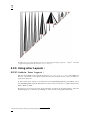
2.2. Main window : Tools bar
8 http://en.wikipedia.org/wiki/Planar_graph
9 http://en.wikipedia.org/wiki/Planar_graph#Outerplanar_graphs
10 http://en.wikipedia.org/wiki/Simple_graph#Simple_graph
11 http://en.wikipedia.org/wiki/Acyclic_Graph
12 http://en.wikipedia.org/wiki/Connected_graph
13 http://en.wikipedia.org/wiki/Biconnected_graph
14 http://en.wikipedia.org/wiki/Directed_tree
4
Graphic
Interface
The tool bar contains 5 tools :
•
Open file : Open a new graph.
•
Save file : Save current graph.
•
Print : Print the current graph.
•
Undo : Undo the last operation on the graph.
•
Redo : Redo the last undo operation.
2.3. Graph Editor
This subwindow is divided in four tabs : Property, Element, Hierarchy, Statistics (not displayed in the
standard version).
2.3.1. Property
This tab enables to display the properties of nodes and edges as a table. It is composed of two parts.
The one of the top of the tab displays all the values of nodes or edges for the selected property (choosen
in the lists at the bottom of the tab). It is possible to display only the values of the selected elements
by using the selected only box. The user can modify directly a value by double-clicking on the
corresponding cell in the table. After editing the value, press the Enter key to update the display of
the graph with the new value. It is possible to set all the nodes or edges value with the Set all
button; if the selected only box is checked, this will only affect the selected elements. An other
possibility is to set as labels the values of the selected property by clicking on the To labels button.
The bottom part of the tab displays the lists of all the local and inherited properties of a graph. An
inherited property is a property which is defined for an upper graph in the hierarchy of graphs (see
Section 2.3.3, “Hierarchy”).
5
Graphic
Interface
By a right mouse button press (press Ctrl key when mouse pressing on Mac) on a row of the table
values, you can display a pop-up menu allowing some actions on the graph element corresponding to
the table row:
• Add to/Remove from selection : this allows to change the selection state of the element,
• Select : the current element replaces the whole selection,
• Delete : this permanently removes the element from the current graph,
• Properties : this shows the element properties in the “Element” tab (see after).
6
Graphic
Interface
For more details please visit : Section 3.3, “Properties of graph”
2.3.2. Element
This tab shows informations about an element of the graph, node or edge, previously "pointed" using
the
mouse toolbar operation. At the top, you can find the type of the element and its “id”. To follow,
here is the table displaying the elements properties and associated values. As within the tables of the
“Property” tab, it is possible to update the values within this table.
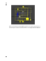
2.3.3. Hierarchy
This tab shows the inclusion relationships betweeen the different existing subgraphs and groups of a
graph. All of them could be created with the Tulip tools. A hierarchy of graph is often the result of
the computation of clustering algorithms.
7
Graphic
Interface
By a right mouse button press (press Ctrl key when mouse pressing on Mac) in the hierarchy display,
you can display a pop-up menu allowing to remove, clone, rename, a graph (subgraph or group).
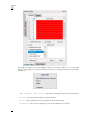
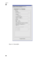
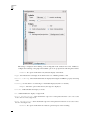
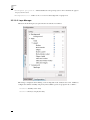
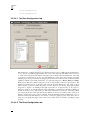
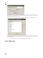
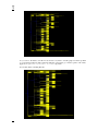
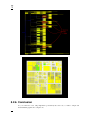
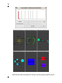
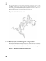
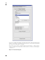
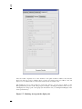
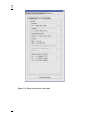
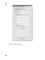
2.3.4. Statistics (not available in standard version)
The statistics panel is composed of three main parts : Computation, Display and Clustering. It allows
the user to compute a histogram or a scatter plot from a graph and one up to three metrics. The display
part of the panel is used to display on screen the statistics main values (as Average point, Standard
deviation, Bounding box, Linear Regression and Eigenvectors). The clustering part is used to display
a clustering plane from a statistical value (previously computed) and to separate the graph into two
new clusters : what is above the clustering plane (sup) and what is under the clustering plane (inf)
Figure 2.1. Computation Tab
8
Graphic
Interface
Figure 2.2. Display Tab
9
Graphic
Interface
Figure 2.3. ClusteringTab
10
Graphic
Interface
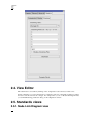
2.4. View Editor
This subwindow is accessible by clicking on the "Configuration" tab at the bottom left corner.
On this subwindow you can found interactor configuration and view configuration. When we change
the active view this window also changes. For example when you are on Node Link Diagram View,
you can find Rendering parameters dialog on this configuration window.
2.5. Standards views
2.5.1. Node Link Diagram view
11
Graphic
Interface
2.5.1.1. Mouse Interaction Toolbar
This toolbar allows to select the mouse operation you want to perform. Operations are listed and
explained, from left to right of the toolbar :
•
3D Navigation : This tool enables the 3D navigation in a graph using the mouse movements (left button
pressed); the available operations are: translate, rotate, zoom, zoom and pan. Translation is the default
operation and can also be activated using the Arrow keys; rotation is activated using Shift key, zoom is
activated using Ctrl key (Alt key on Mac), zoom and pan is activated using the wheel of the mouse (APPLE
key on Mac). Warning, the last operation is ’mouse position centered’; i.e it attempts to translate the last 2D
or 3D position of the mouse to the center of the view.
•
Get Information : when this operation is selected, if you click on an element of a graph (node or edge),
Tulip displays all available properties of that node/edge using the Element tab of the Info Editor subwindow (see Section 2.3, “Graph Editor”).
•
Rectangle Selection : Allows multiple elements selection. Elements within the selection box are
selected. If Shift key is pressed, the newly selected elements are added to the current selection, if Ctrl key
(Alt key on Mac) is pressed, the selected elements are removed from the current selection; else they replace
the current selection.
•
Selection edition : This tool allows to modify the current selection. Available operations are
horizontal stretch, vertical stretch, all axis stretch, coordinate axis rotation and translation. If no key is pressed,
coordinates are modified. If Shift key is pressed, only coordinates are modified. If Ctrl is pressed, only size
is modified. A left button click outside the selection box reset the selection.
•
Press on this ’circle’ to rotate the selection.
•
Press on this ’triangle’ to change width or height of the selection.
•
The ’square’ is used both for resizing AND rotating the selection.
12
Graphic
Interface
•
Magic Selection : It enables to select all the graph connected nodes having the same metric. It works
like the magic selection in image editing software. The difference is the topology of the graph.
•
Zoom Box : It enables to zoom on a defined rectangle area. The first corner of the rectangle is defined when
pressing the mouse left button, the opposite corner is defined when moving the mouse and the zoom operation
is performed on the desired rectangle when the button is released.
•
Delete element : allows to delete a node or edge by a single left click. The deleted node or edge is the
one under the mouse when you click.
•
Add node : when it is selected, you can add a node in the graph by a simple left mouse click on the current
graph view. The node is placed at the coordinates corresponding to the mouse position when you clicked.
•
Add edge : when it is selected, you can add an edge in the graph by mouse left clicking first on the source
node then any left click will add a bend to the edge until a left click on the target node.
•
Edit edge bends : when it is selected, you can edit the bends of an edge by first selecting the edge using
the mouse left button. Then a mouse left click with the Shift key pressed will add a new bend, moving the
mouse with the left button pressed will allow to move an existing one, a mouse left click on a bend with the
Ctrl key pressed (Alt key on Mac) will remove it.
2.5.1.2. View window
13
Graphic
Interface
The 3D graph view subwindow is the window where the graph is displayed. It can display graph in
two or three dimensions and enables to apply the mouse operations selected in the tool bar by directly
clicking on the drawing of the graph. If the user lets the mouse during few seconds on a node/edge, a
tooltip window displays its id and label (use “Options” menu to enable tooltips).
2.5.1.2.1. Pop-up menu of graph view
This pop-up menu is displayed when pressing on the mouse right button (press Ctrl key when mouse
pressing on Mac) :
• View -> Redraw view : redraw the view,
• View -> Center view : center the current graph in the view,
• Dialog -> 3D Overview : display/hide top left overview,
14
Graphic
Interface
• Dialog -> Augmented Display : manage augmented display of the graph (for example :
caption when we apply a color algorithm),
• Options -> Tooltips : enables the display of tooltips on nodes or edges,
• Options -> Grid : shows the grid configuration dialog.
• Options -> Z Ordering :
nodes/edges.
Use this option when you have graph with transparent
• Options -> Antialiasing : enable/disable antialiasing.
• Options -> Textured meta node : enable/disable meta node texture rendering.
• Save picture as -> ... : to save the graph picture in multiple format.
If you press right button of the mouse when your pointer is on a graph element, you have this context
menu to perform simple actions on this element :
• Add to/Remove from selection : this allows to change the selection state of the element,
• Select : the current element replaces the whole selection,
• Delete : this permanently removes the element from the current graph,
• Go inside : if the element is a metanode, this shows the corresponding subgraph in the current
view,
• Ungroup : if the element is a metanode, this permanently removes it and its corresponding
subgraph,
• Properties : this shows the element properties in the “Element” tab.
2.5.1.3. Rendering Parameters
2.5.1.3.1. Parameters
All actions in this dialog are just performed for the current view window.
15
Graphic
Interface
This dialog is displayed when clicking on the Configuration tab at button left corner. Enables to
configure the rendering of the graph. The available options are grouped in the following three frames:
• Labels : the options in this frame only affect the display of the labels:
• Type : this indicates the text display mode which can be one of Bitmap, Texture or 3D.
• metric ordering : when checked the labels are displayed in using the viewMetric property decreasing
order.
• Density : use this slider to avoid having too much labels displayed (max is on the left).
• Edges : this frame options affect the way the edges are displayed:
• arrows : enables/disables the display of arrows.
• 3D : enables/disables the display of edges in 3D.
• Color interpolation : when checked the edge color is interpolated from the color of its source
node to the color of its target node.
• Size interpolation : when checked the edge size is interpolated from the size of its source node to
the size of its target node.
• Others : the options in this frame are related to general aspects of the rendering:
16
Graphic
Interface
• Orthogonal projection : enables/disables the orthogonal projection. If not checked, the perpsective projection is used.
• Background color : enables to choose a color for the background of a graph view.
2.5.1.3.2. Layer Manager
All actions in this dialog are just performed for the current view window.
This dialog is displayed when clicking on the Configuration tab at button left corner. Enables to
configure the elements visibility and priority. The available options are grouped in two columns :
• Visible : Visibility of the entity
• Stencil : Priority to display the entity
17
Graphic
Interface
In this menu, you see Hull entity, it represents the convex hulls of the graph. When you click on
visible, a hierarchy of convex hulls is build. The name of a hull is the name of the coresponding
subgraph.
In a future version you could add/modify/remove entity
2.5.2. Parallel Coordinates view
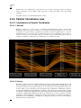
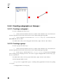
2.5.2.1. Introduction to Parallel Coordinates
2.5.2.1.1. Concept
Parallel coordinates is a common way of visualizing high-dimensional geometry and analyzing
multivariate data. The idea is to visualize a set of points in an n-dimensional space. To do so, the
n dimensions are represented by n parallel axis, typically vertical and equally spaced. A point in
n-dimensional space is represented as a polyline with vertices on the parallel axis. The position of
the vertex on the i-th axis corresponds to the i-th coordinate of the point. The image below shows an
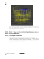
example of a parallel coordinates plot for visualizing a set of 5-dimensions data.
2.5.2.1.2. History
Parallel Coordinates were firstly studied by Maurice d’Ocagne in 1885 [Ocagne1885] (mostly for 2-D
use in Nomography) and were popularised by Al Inselberg [Inselberg85]. The first Multidimensional
Coordinate System was developed by this last one in 1977 based on his independent rediscovery
in 1959. Many people contributed to the development and popularization of Parallel Coordinates.
Among them, Ed Wegman applied Parallel Coordinates to data exploration, and particularly visualize
correlations in datasets. His landmark paper entitled "Hyperdimensional Data Analysis Using Parallel
Coordinates" [Wegman90], published in 1990, is the starting point of concrete parellel coordinates
applications. Today applications of Parallel Coordinates are in Collision Avoidance Algorithms for
Air Traffic Control, Data Mining , Computer Vision, Optimization, Process Control, more recently in
Intrusion Detection and elsewhere.
18
Graphic
Interface
[Ocagne1885] “Coordonnées parallèles et axiales: Méthode de transformation géométrique et procédé nouveau
de calcul graphique déduits de la considération des coordonnées parallèlles”. Maurice d’Ocagne.
1429700971. Cornell University Library. Copyright © 1885.
[Inselberg85] The Visual Computer. 0178-2789. Springer Berlin / Heidelberg. Copyright © 1985. 1. 4. “The
Plane with Parallel Coordinates”. Al Inselberg. 69-91.
[Wegman90] Journal of the American Statistical Association. 0162-1459. American Statistical Association.
Copyright © 1990. 85. 411. “Hyperdimensional data analysis using parallel coordinates”. Ed Wegman.
664-675.
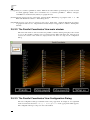
2.5.2.2. The Parallel Coordinates View main window
This is the main window of the view where the parallel coordinates drawing is displayed. It is created
as soon as the parallel coordinates view is requested via the Tulip main menu bar. After the view
creation, the content of this window is empty and the view has to be setup via the configuration
dialog.
2.5.2.3. The Parallel Coordinates View Configuration Dialog
The view configuration dialog is reachable via the view popup menu. To display it, do a right-click
in the view window and select Dialog -> Configuration in the popup menu which appears.
The configuration dialog is composed of two tabs entitled:
19
Graphic
Interface
• Data Configuration
• Draw Configuration
2.5.2.3.1. The Data Configuration tab
This tab allows to configure the data to plot. Because the data source is a Tulip graph, the first thing to
do is to precize from which graph elements, the nodes or the edges, the data will be retrieved. To do
so, click on the appropriate radio button in the upper part of the tab. Next, the dimensions of the data
to plot have to be selected. In our case, the data dimensions corresponds to the properties associated
with the graph. At the present time, the graph properties that can be selected to be visualized with the
parallel coordinates representation must have one of the following types : Metric, Integer or String.
Each selected dimension will be mapped to an axis in the parallel coordinates representation. The
dimensions selection is done on the lower part of the tab. To add a dimension to plot, click on one of
them in the list on the left (entitled "Properties to hide") and move it in the list on the right (entitled
"Properties to display") by clicking in the right arrow button or by drag and drop it. To remove a
dimension, click on one of them in the list on the right and move it in the list on the left by clicking on
the left arrow button or by drag and drop it. The selected dimensions can also be ordered by picking
one of them in the list on the right and then by clicking on the up arrow button or the down arrow
button to change the property position in the list. In the drawing that will be generated, the colors of
the lines between axis will be those stored in the "viewColor" graph property. If the data source is
the nodes of the graph, the shapes of the points on axis will be those stored in the "viewShape" graph
property.
2.5.2.3.2. The Draw Configuration tab
20
Graphic
Interface
In this tab, many parameters relative to the parallel coordinates drawing can be set. Let’s make a
review of them.
• General draw parameters
• Background color : allow to set the view background color. To do so, click on the colored button
and pick a color in the color dialog which appears
• Axis Height : allow to set the height of the different axis
• Space between axis : allow to set the space between the different axis
• Lines color alpha value : allow to set the transparency level of lines representing data. The
minimum value is 0 (totally transparent) and the maximum is 255 (opaque)
• Draw points on axis If this group box is checked, points corresponding to dimensions
values on axis will be drawn. This option is desactivated by default when the number of data to plot is greater
than 5000 in order to speed up the rendering process. The size of points on axis is proportionnal to the
"viewSize" property value. The minimum and maximum point size can be set freely by using the spinbox
contained in the group box. The minimum "viewSize" value will be mapped to the minimum point size and
the maximum "viewSize" value will be mapped to the maximum point size.
• Apply texture on lines If this group box is checked, a texture will be applied on the lines
representing data. Two choices are proposed :
• Use Tulip default texture : use the default parallel coordinates view texture proposed by Tulip.
This texture is applied on the alpha channel of the lines colors.
• Use texture from file : apply a personnal texture from an image file (width and height of the
image must be a power of 2)
21
Graphic
Interface
2.5.2.4. Tulip Parallel Coordinates View Interactors
To play with the view, a few number of interactors can be found in the following toolbar :
Let’s introduce them and their functionnalities.
•
View Navigator : This interactor enables the 3D navigation on the view using the mouse movements
(left button pressed). Its working is the same as the 3D Navigator interactor from the Node Link Diagram
Component (see Node Link Diagram 3D Navigator).
•
Zoom Box : This interactor enables to define a zoom area with the mouse. Its working is the same as the
Zoom Box interactor from the Node Link Diagram Component (see Node Link Diagram Zoom Box).
•
Show Element Properties : This interactor allows to view the properties associated to an element by
clicking on it. Tulip will display all available properties of that node/edge using the Element tab of the Info
Editor sub-window (see Section 2.3, “Graph Editor”)
•
Elements Selector : This interactor allows to select elements in the parallel coordinates view. Its
working is the same as the Rectangle Selection interactor from the Node Link Diagram Component
(see Node Link Diagram Rectangle Selection).
•
Element Deleter : This interactor allows to remove from the parallel coordinates view all the elements
under the mouse pointer after a left-click.
•
Element Highlighter : This interactor allows to highlight elements in the parallel coordinates view.
When an element is highlighted, it keeps its original color and the other elements are colored in gray. A
left-click in the view will highlight all the elements under the mouse pointer. It is also possible to define a
rectangular region with the mouse to highlight all elements in that region. If there is no elements under the
mouse pointer while clicking, the whole highlighted elements set will be reseted and all elements will get back
its original color. By maintaining the Shift key while clicking, the elements under the mouse pointer will be
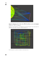
add/remove from the current highlighted elements. Below is an example of the element highlighter interactor
result. Image on the left shows a parallel coordinates view without highlighted elements. By clicking on the
element that has the maximum value for the "#hands" dimension, it will be highlighted and the result is shown
on the image on the right.
22
Graphic
Interface
•
Axis Swapper : This interactor allows to swap two axis with the mouse in the parallel coordinates drawing.
To do so, put the mouse pointer under the axis you want to swap, a translucent blue rectangle will be drawn
to indicate that you can click to move the axis. Once the pointer is under the axis, do a left click and keep
the mouse button pressed while you’re dragging the axis. To swap the axis with an other, release the mouse
button when a translucent green rectangle appears around the other axis to swap. The image below illustrates
this process.
23
Graphic
Interface
•
Axis Sliders : This interactor allows to select a range on a particular axis with the help of sliders and
highlight all the data located in that range. This operation allows to filter data according to a certain dimension.
24
Graphic
Interface
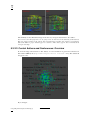
To use the axis sliders, put the mouse pointer under the one you want to move (the slider outline color will
change), do a left-click and drag the slider along the axis. Release the mouse button when the slider is at the
wanted position, the data located between the two axis sliders will be automatically highlighted. The sliders
of the axis whose range has been modified will be colored in blue to indicate on which dimension the data
filtering is made. The other axis sliders will also move automatically to show in which ranges the highlighted
data are included on the other dimensions. It is also possible to drag the range defined by two axis sliders, by
putting the mouse pointer between them (a translucent rectangle will appear) and drag and drop it along the
axis. The image below shows the result of this interactor after filtering data on the "#hands" dimension.
•
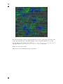
Axis Box Plot : By enabling this interactor, a box plot will be drawn above each quantitative axis. In
descriptive statistics, a boxplot (also known as a box-and-whisker diagram or plot) is a convenient way of
graphically depicting groups of numerical data through their five-number summaries (the bottom outlier, first
quartile (Q1), median (Q2), third (Q3), and the top outlier). The image below illustrates the way to read a box
plot.
25
Graphic
Interface
A boxplot may also indicate which observations, if any, might be considered outliers. The boxplot was invented
in 1977 by the American statistician John Tukey. Boxplots can be useful to display differences between
populations without making any assumptions of the underlying statistical distribution. The spacings between
the different parts of the box help indicate the degree of dispersion (spread) and skewness in the data, and
identify outliers.It is possible to highlight data included in the following axis box plot range :
• [Bottom Outlier, First Quartile]
• [First Quartile, Median]
• [Median, Third Quartile]
• [First Quartile, Third Quartile] (= interquartile range)
• [Third Quartile, Top Outlier]
To do so, put the mouse pointer between the two bounds of the wanted range, a translucent rectangle will
be drawn to indicate it is selected, and do a left-click to highlight data. To highlight the data included in the
interquartile range, put the mouse pointer near the median line and the interquartile range will be selected. The
following screenshot illustrates this interactor.
26
Graphic
Interface
2.5.2.5. The Parallel Coordinates View popup menu
By right-clicking in the parallel coordinates main window, a popup menu will be displayed. The
content of it depends on the location of the mouse pointer. By default, the following menu is displayed
:
The entries it contained are the following :
• Dialog -> Configuration : Display the parallel coordinates view configuration dialog
• View Setup -> Center View : Center the parallel coordinates drawing inside the view
main window
• View Setup -> Classic View : By clicking on this menu entry, the parallel coordinates
will be drawn the classic way with straight lines between axis. This view mode is the default one.
• View Setup -> Spline View : By clicking on this menu entry, the parallel coordinates
will be drawn with bezier curves between axis. Beware because this view mode is not optimized for
performance, the drawing computing and the rendering process can be really slow if there’s more than a
thousand of data to plot.
• Options -> Tooltips : By enabling this option, when the mouse pointer is under an
element a tooltip message will be displayed containing the element label (if there is one set in the "viewLabel"
property) and the element id.
27
Graphic
Interface
If there is highlighted elements in the drawing (set with the elements highlighter or the axis sliders
interactors), the following menu entries will be add to the view popup menu.
• Select Highlighted Elements : By clicking on this entry, all the current highlighted
elements will be added to the selected elements set.
• Reset Highlighted Elements : Empty the highlighted elements set. All elements will
get back their original colors.
If there is an element under the mouse pointer when right-clicking, the popup menu will contain
additional entries introduced below.
• Add / Remove From Selection : Add or Remove the pointed element to the selected data
set.
• Select : Empty the selected data set then add the pointed element to it.
• Delete : Delete the pointed data.
• Properties : Display all the available properties of the pointed data in the Element tab of
the Info Editor sub-window (see Section 2.3, “Graph Editor”).
Eventually, if there is an axis under the mouse pointer, the popup menu will contain the following
menu entries.
• Axis Configuration : By clicking on this entry, a dialog will appear to set some axis
parameters. The content of this dialog depends on the axis type.
• For the Quantitative Axis (axis associated to a property whose type is Integer or Metric), the
displayed dialog is the following :
28
Graphic
Interface
This dialog allows to set the number of axis graduations, the axis order (if it is ascending, the minimum
value will be at the bottom of the axis and the maximum one at the top) and it is also possible to set a
logarithmic scale (in base 10) for the axis.
• For the Nominative Axis (axis associated to a property of type String), the dialog is the one below :
This dialog allows to define the axis labels order. To move a label at a certain position, click on it in the
list at the center of the dialog and move it to the wanted position with the help of the arrow buttons on the
right side of the dialog.
• Remove Axis : Remove the axis from the parallel coordinates drawing.
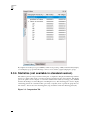
2.5.3. Table view
29
Graphic
Interface
In this view you can visualize graph properties in a table form.
You have two tabs : Node and Edge.
Color of a cell depends on the value of the viewColor property of the node/edge and the color of the
text depends on the value of the viewLabelColor property of the node./edge
30
Chapter 3. Functionalities
3.1. Management of Graphs
Tulip software offers a way to create and manage graphs. The main window enables to have several
3D views to show differents graphs. The menu bar enables the user to create a new view. In there and
with the mouse toolbar, the users can create nodes and edges at the place where the pointer is. When
you have a graph and you want to keep traces of the graph, you can save it in the .tlp format, of
Tulip Software. An other option is to export it in the GML format, for the graphlet system, a toolkit
for graph editors and graph algorithms. Then, you can save as an picture the result you had. Tulip
supports different formats : BMP, EPS, JPEG, PBM, PGM, PNG, PPM, SVG, XBM, XPM.
Tulip could generate a graph from data : importation.
Examples of importation
• Adjacency Matrix : a form of representation of graphs. Please visit Wikipedia: Adjacency Matrix1
for more details.
• File System : make a graph with your file system ; the root is the directory you have selected.
• GML import : create a graph from this other format.
• dot : create a graph from graphviz format.
The second possibility is to generate automatically different kinds of graph : Graph, Tree, Grid, which
could be complete, simple, uniform, ...
Examples of generation
• Complete General Graph
• Complete Tree
• Grid
• Grid approximation
• Random General Graph
• Random Simple Graph
• Uniform Random Binary Tree
1 http://en.wikipedia.org/wiki/Adjacency_matrix
31
Functionalities
It is posssible to do a “Copy-Paste”. You can cut, copy and paste selected elements from a view.
When you paste an element, it is placed at the same location it was in the original view. Use
View->Center View (Ctrl+Shift+C) to make it visible in the second view. The menus and the
mouse toolbar allow you to select the operation you want to perform on the selection.
3.1.1. The “Find” tool
In the Edit menu, it exists a Find item allowing to do some requests on the current graph. The
tool gives a way to choose the desired property and the action you want perform regarding the current
selection: Make out of the found elements a new selection, Add them to the selection, Remove them
from the selection or Intersect them with the current selection.
3.2. Algorithms
Each graph can be modified with algorithms for the layout, the set of selected elements, the size of
nodes, the value attributed to an element (node or edge) named metric, the colors. An other advantage
of Tulip is that it is easy to add a new algorithm in the structure; this way, it is able to include lot of
algorithms. As explain in the Section 2.1, “Main window : Menus”, the algorithms are accessed by
the Algorithms menu. Several categories are in there : Selection, Color, Layout, Measure, Size,
General. They modify the properties of the graph elements.
3.2.1. Selection Algorithms
3.2.1.1. Induced Sub-Graph :
The induced Sub-Graph algorithm can be used to obtain the edges that are between selected nodes.
Here is an example :
Before :
After :
32
Functionalities
Algorithm documentation2
3.2.1.2. Kruskal :
The Algorithm of Kruskal is used to create a minimum spanning tree out of a connected graph.
It is divided in several steps :
• Make a list of the edges starting with the "shortest" one, ending with the "longest one".
• Add all edges with their from/to nodes to the tree as long as you don’t have any cycle.
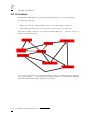
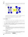
Let’s take an example : We have a set of airports, Bordeaux, Paris, L.A ..., the nodes, and a set of
Airports connections, the edges.
As you can see, this makes a very complicated Graph. As edges do not all have the same weight (in
terms of price, distance, ...), some of them are not really important (the ones with a high weight). The
algorithm of kruskal will select the ones that we can’t remove.
2 ../../doxygen/allPlugins.html#InducedSubGraphSelection
33
Functionalities
By creating a sub-graph we get a simple graph which is much more easy to read.
Please visit Wikipedia : Kruskal’s algorithm 3 for more details.
Algorithm documentation4
3.2.1.3. Loop Selection :
This selection algorithm is able to select the loops of a graph. A loop is an edge that has the same
source and target.
3 http://en.wikipedia.org/wiki/Kruskal%27s_algorithm
4 ../../doxygen/allPlugins.html#Kruskal
34
Functionalities
Algorithm documentation5
3.2.1.4. Multiple Edge :
This selection algorithm highlights the multiple-edges also named parallel-edges in a graph.
Two edges are parallel only if they both have the same target and same source.
Algorithm documentation6
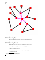
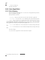
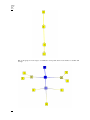
3.2.1.5. Reachable Sub-Graph :
This selection algorithm enables to find all nodes and edges at a fixed distance of a set of nodes. It
takes three parameters :
• Distance : number of edges to follow.
• Direction : 0 means directed, 1 reverse directed, 2 undirected
• Starting nodes : the selected nodes of this selection property ( boolean ) will be used as
starting nodes.
In the following example, ’distance’ equals to 1, ’direction’ equals 0, and the starting node is the one
in the center.
Before :
5 ../../doxygen/allPlugins.html#LoopSelection
6 ../../doxygen/allPlugins.html#MultipleEdgeSelection
35
Functionalities
After :
36
Functionalities
Algorithm documentation7
3.2.1.6. Spanning Dag :
This selection algorithm can be used to select a sub-graph without any cycle.
Algorithm documentation8
3.2.1.7. Spanning Forest :
This algorithm can be used to create a set of spanning trees out of the graph.
A tree is a special kind of graph that has the following properties :
• Has a root (a starting point node).
• A node have severals sons and their is only one edges targeting each sons.
• Doesn’t have any cycle.
7 ../../doxygen/allPlugins.html#ReachableSubGraphSelection
8 ../../doxygen/allPlugins.html#SpanningDagSelection
37
Functionalities
• A leaf is an "ending node".
Algorithm documentation9
3.2.2. Color Algorithms :
3.2.2.1. Metric Mapping :
The metric mapping algorithm can be used to re-color the nodes of the graph after using a measure (
Section 3.2.3, “Measure” ) algorithm.
This Algorithm takes 5 parameters :
• Property : Property is a metric value. It is used to affect scalar values to graph items.
• Colormodel : Color can be either 1 or 0. 1 for RGB interpolation and 0 for HSV interpolation.
• Type : If type is checked, the color mapping will be uniform, which means that if you have 2
nodes with the property value equals to 0, there will be 2 nodes colored in "color1" . If type is not checked,
the color quantification will be linear, which means that if you have 2 nodes with the property value equals to
0, there will be 1 node colored in "color1" and an other with a lighter color1.
• Color1 : Color1 will be the color of the node that has the lowest value (according to the Property
field)
• Color2 : Color2 will be the color of the node that has the highest value (according to the Property
field)
Let’s take an example :
As you can see here is a graph where no metric values has been computed.
9 ../../doxygen/allPlugins.html#SpanningTreeSelection
38
Functionalities
After applying the degree algorithm, the graph gets colors !
39
Functionalities
If you do not have any colors (on edges), see if you have checked the "Color interpolation" in the
rendering parameters window ( CTRL+R) . After applying the "Metric mapping" algorithm ("type"
checked, "colormodel" equaled to 1 , "Color1", a kind of red and "Color2" a kind of green ) we will
obtain the following graph.
40
Functionalities
3.2.3. Measure
Measure algorithms are used to compute different metrics (on edges or nodes). The computed values
are assigned to the viewMetric property.
3.2.3.1. Graph :
3.2.3.1.1. Betweenness Centrality :
Betweenness is a centrality measure of a node within a graph. Nodes that occur on many shortest
paths between other nodes, have higher betweenness metric than those that do not. As this algorithm
will compute a global measure, it can take a long time to finish. See Widipedia : Betweenness10 for
more details.
Algorithm documentation11
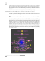
3.2.3.1.2. Cluster :
This algorithm can only be used on simple graphs (graphs with no loops).
10 http://en.wikipedia.org/wiki/Betweenness
11 ../../doxygen/allPlugins.html#BetweennessCentrality
41
Functionalities
The cluster algorithm is a measure algorithm that can determine whether or not a graph is a "smallworld network". The clustering measure is a local measure that gives the connections rate of a node
and its neighbors.
Let’s take an example :
On this graph, and by looking at the clustering measure, you can see 2 "communities" (nodes in blue)
and a hub (node in yellow).the hub is the only way to connect the two communities.
For more details, please visit http://en.wikipedia.org/wiki/Clustering_coefficient.
Algorithm documentation12
3.2.3.1.3. Degree :
This algorithm will save the degree of each node in its viewMetric property. It takes two parameters :
• Type : Is the type of degree you want to compute. In : Edges that comes onto the node. Out :
Edges that are going away from the node. InOut : Using both (in and out).
• Metric : This parameter can take all double properties, but by default it will take : None,
’viewBorderWidth’, ’viewMetric’ and ’viewRotation’. If you choose none, the degree of the node will be
the sum of the edges. If you choose the ’viewMetric’ value, degree of the node will be the sum of edges
wiewMetric property. As of viewBorderWidth and viewRotation.
3.2.3.1.4. Eccentricity :
This plug in compute the eccentricity of each node, eccentricity is the maximum distance to go from
a node to all others. In this version the value is normalized (1 means that a node is in the center of the
network, 0 means that a node is the more eccentric in the network). The eccentricity will be saved in
the viewMetric property of each node.
Algorithm documentation13
3.2.3.1.5. Strahler :
The Strahler algorithm is very powerful. It can for example point out important path in a graph, by
computing for each node the degree of ramification of its (spanning) sub-tree. Following is a graph
with only one path. You can see that each node have the same Strahler number (1).
12 ../../doxygen/allPlugins.html#ClusterMetric
13 ../../doxygen/allPlugins.html#EccentricityMetric
42
Functionalities
But on this graph, more the degree of ramification is important and more the number of strahler will
be high.
43
Functionalities
Note that this graph could represent anything, a program (inclusion of sources files), or a city road
traffic.
Parameters :
• All nodes : If not checked, the algorithm will choose a node (a source node) and will apply
the algorithm to this node only. If checked, the algorithm will be applied to all nodes.
• Type :This parameter can take 3 different values : Register which will force the algorithm to
give an indication on the degree of ramification (for trees), Stack, that will force the algorithm to give an
indication on the number of nested cycles (for graphs), and at last, All, that will ask the algorithm to use both
registers and stack.
For more information please visit http://en.wikipedia.org/wiki/Strahler_Stream_Order
Algorithm documentation14
3.2.3.1.6. Strength :
Graph must be simple (no loops).
This algorithm will compute the strength of edges. Every edges with small values are important in
the way that their removal can disconnect two connected components. Every edges with a high value
metric may belong to a strongly connected component.
Algorithm documentation15
3.2.3.2. Component :
3.2.3.2.1. Biconnected Component :
A connected graph is biconnected if the removal of any single node and his edges can not disconnect
the graph. The biconnected components of a graph are the maximal subsets of nodes such that the
removal of a node from a particular component will not disconnect the component. Note that unlike
connected components, a node can belong to multiple biconnected components. For example we can
use this algorithm on an airlines graph. Such as the one following.
14 ../../doxygen/allPlugins.html#StrahlerMetric
15 ../../doxygen/allPlugins.html#StrengthMetric
44
Functionalities
The result is, 3 biconnected components :
• : Paris, New York, L.A, Madrid.
• : Paris, Berlin.
• : Berlin, Moscow, Prague.
45
Functionalities
The intersection of those 3 biconnected components is Berlin and Paris. Which means that Berlin and
Paris are two articulation points of our graph.
Algorithm documentation16
3.2.3.2.2. Connected Component:
A connected component is a maximal connected subgraph. Two nodes are in the same connected
component if and only if there exists a path between them.
After running the algorithm, the index of the connected component of a node is saved in its viewMetric
property. It is the same for the edges.
For more details please visit : Wikipedia:Connected Component17 Algorithm documentation18
3.2.3.2.3. Connected Tree Component :
The connected tree component algorithm can be useful to find parts of a graph that are trees. Here is
an example :
Following is a graph with on the left side, a tree. This graph forms a unique connected component.
As you can see, the algorithm divided the graph into 2 components.
16 ../../doxygen/allPlugins.html#BiconnectedComponnent
17 http://en.wikipedia.org/wiki/Connected_component_(graph_theory)
18 ../../doxygen/allPlugins.html#ConnectedComponent
46
Functionalities
Algorithm documentation19
3.2.3.2.4. Strongly Connected Component :
A directed graph is said to be strongly connected if for every pair of nodes S1 and S2, it exists two
edges e1 and e2 such as :
• The Source of e1 is S1 and Target is S2 .
• The Source of e2 is S2 and Target is S1.
The strongly connected components of a directed graph are its maximal strongly connected subgraphs.
These form a partition of the graph. Here is an example :
Before :
19 ../../doxygen/allPlugins.html#ConnectedAndTreeComponent
47
Functionalities
After :
3.2.3.3. Tree
To use the following algorithms the graph has to be acyclic. A graph is acyclic if it contains no cycle.
3.2.3.3.1. Dag Level
The dag level algorithm will compute the depth of each node, as on the following example :
48
Functionalities
Algorithm documentation20
3.2.3.3.2. Depth
The depth algorithm will compute for each node, the maximum number of edges to follow to find a
leaf.
Algorithm documentation21
3.2.3.3.3. Leaf
The leaf algorithm will compute for each node its number of leaves.
Here is an example :
20 ../../doxygen/allPlugins.html#DagLevelMetric
21 ../../doxygen/allPlugins.html#DagLevelMetric
49
Functionalities
Algorithm documentation22
3.2.3.3.4. Node
The Node algorithm, will sum for each node the number of its children nodes plus him self. Algorithm
documentation23
3.2.3.3.5. Path Length
This algorithm will count for each node the number of paths that goes through it.
Here is an example :
22 ../../doxygen/allPlugins.html#LeafMetric
23 ../../doxygen/allPlugins.html#NodeMetric
50
Functionalities
3.2.3.3.6. Segment
A segment, is a set of nodes that are all on one and only path. The graph showed on the left side of
the example is a segment.
The segment algorithm will count, for all nodes, its number of edges without ramification.
Following are two graphs. On the left one you can see that the root "has" 3 edges without ramification.
But, on the right graph all nodes (without considering leaves) have only 1 edge without ramification.
51
Functionalities
This algorithm can be useful to see how the graph is formed. Indeed, if the root has a small value, it
will mean that the graph has a "good" ramification. But if the root has a high value, it will mean that
the graph a lot of segments.
3.2.3.3.7. Tree Arity Max
Compute the maximum outdegree of the nodes in the subtree induced by each node. To access to
the degree of a node it is recommended to use directly the degree function available in each Graph.
Algorithm documentation24
3.2.3.4. Misc
3.2.3.4.1. Id
The "id" algorithm will, for each node and edge, save their id number in their viewMetric Property.
For example, if we have a node called Node 9, its id number will be 9. Algorithm documentation25
3.2.3.4.2. Random
Random will just save a random number (from 0 to 1) in the viewMetric property of each node and
edges Algorithm documentation26
3.2.4. Layout
Warning !
checked.
: Some of the following algorithm have no effect if the option "Force Ratio" is
3.2.4.1. Planar
3.2.4.1.1. 3-Connected (Tutte)
This algorithm can only be applied to 3-connected graphs. A graph G is said to be 3-connected if there
does not exist a set of 2 nodes whose removal disconnects the graph. (Triangle Layout) Algorithm
documentation27
3.2.4.1.2. Mixed Model
Create a planar sub-graph with polylines with a good angular resolution which will make the graph
clear and easy to read. Algorithm documentation28
24
25
26
27
28
../../doxygen/allPlugins.html#TreeArityMax
../../doxygen/allPlugins.html#IdMetric
../../doxygen/allPlugins.html#RandomMetric
../../doxygen/allPlugins.html#Tutte
../../doxygen/allPlugins.html#MixedModel
52
Functionalities
3.2.4.2. Tree
To represent a tree, a hierarchical layout is the easiest way to understand the tree structure. But this
layout has a big weakness when the tree has a lot of nodes : it does not effectively use the space where
the tree is displayed. That is why we need different layouts.
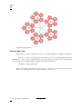
3.2.4.2.1. Bubble Tree
The Bubble Tree algorithm can be use to change the layout of a tree. On the new layout, a node will
be on the center of a circle, and its children will be on the circle. This new layout has the following
properties :
• The edges should not cross each other.
• The polyline used to draw an edge should have the least possible bends.
• The minimal angle between two adjacent edges of a node n should be nearest to 2pi / deg (n). This
property will improve the angular resolution.
• The order of children of a node should be respected in the final drawing.
Here is an example :
The following graph has the default layout (hierarchical layout). It has a pretty bad angular resolution.
Indeed, we do not see the leaves, but only a large black rectangle of edges.
Here is the same tree with a Bubble Tree layout. The angular resolution is much better.
53
Functionalities
Algorithm documentation29
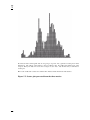
3.2.4.2.2. Cone Tree
The cone tree is a 3d layout which seen from the top, looks like a bubble tree. It takes two parameters:
• node size : size of the node will depend of the metric that you choose. The Algorithm will consider
that parameter so that no nodes overlap themselves. This can be useful, if you want a node to be far from the
others, just take a new size Metric and give a higher value to that specific node.
• Orientation : Vertical / Horizontal
Here is an example of this layout. On the left side you can see a tree with a hierarchical (classic)
layout, and, on the right side, the same tree, but with a cone tree layout.
29 ../../doxygen/allPlugins.html#BubbleTree
54
Functionalities
Algorithm documentation30
3.2.4.2.3. Dendrogram
The dendrogram layout is a hierarchical layout on which every leaves are displayed on the same layer.
A dendrogram is a tree diagram frequently used to illustrate the arrangement of the clusters produced
by a clustering algorithm. Dendrograms are often used in computational biology to illustrate the
clustering of genes.
The algorithm takes 4 parameters :
• node size : size of the node will depend of the metric that you choose. The Algorithm will consider
that parameter so that no nodes overlap themselves. This can be useful, if you want a node to be far from the
others, just take a new size Metric and give a higher value to that specific node.
• orientation : up to down, left to right, right to left or down to up.
• layer spacing : space between the levels of the Tree.
• node spacing : space between sibling nodes.
30 ../../doxygen/allPlugins.html#ConeTreeExtended
55
Functionalities
Algorithm documentation31
3.2.4.2.4. Hierarchical Tree (R-T Extended)
The hierarchical tree layout looks the same that the dendrogram layout or the improved walker layout
but takes an other parameter, "edge length".
• node size : size of the node will depend of the metric that you choose. The Algorithm will consider
this parameter so that no nodes overlap themselves. This can be useful, if you want a node to be far from the
others, just take a new size Metric and give a higher value to that specific node.
• edge length : this parameter can take a property of type int, and will be used to place a node on a
specific layer. If its value is 1, no thing will happen, but if its value is 2, the node will be placed on the next
layer.
• orientation : vertical/horizontal;
• orthogonal : enables the drawing of the edges, orthogonally bent.
• layer spacing : space between the levels of the Tree.
• node spacing : space between nodes sibling nodes.
• bounding circle : if checked, the estimation of overlapping nodes will be computed with bounding
circles instead of bounding rectangles.
Algorithm documentation32
3.2.4.2.5. Improved Walker
The improved walker layout is just a hierarchical layout. Algorithm documentation33
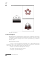
3.2.4.2.6. Squarified Tree Map
The squarified tree map layout, will place nodes in nested rectangles. For example, lets take a tree
with a root and two sons, the layout will draw a rectangle for the root containing two other rectangles
(its sons). This layout can be very useful for analyzing disks usages.
Here is an example :
Following is the tree a a file system containing 6 file of 1Mb, and severals directories.
31 ../../doxygen/allPlugins.html#Dendrogram
32 ../../doxygen/allPlugins.html#TreeReingoldAndTilfordExtended
33 ../../doxygen/allPlugins.html#ImprovedWalker
56
Functionalities
The same graph, with a squarified tree map layout :
Using the 3D, we can see how the layout is done :
57
Functionalities
Algorithm documentation34
3.2.4.2.7. Tree Leaf
This layout looks like the improved walker, but does not pack the nodes. The result is a nice
hierarchical tree in which nodes does not overlap. Algorithm documentation35
3.2.4.2.8. Tree Map (Shneiderman)
This layout, is the same as the squarified tree map layout, but the squarified tree map uses shadows to
draw the tree. Algorithm documentation36
3.2.4.2.9. Tree Radial
On this layout, nodes of the same layer are placed on a circle whose center is the root. Algorithm
documentation37
3.2.4.3. Basic
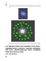
3.2.4.3.1. Circular
On this layout, every nodes are placed on a circle. Algorithm documentation38
3.2.4.3.2. Random
Nodes are placed randomly in space.
3.2.4.4. Misc
3.2.4.4.1. Connected Component Packing
This layout groups connected components of the graph so that they do not overlap themselves and that
lost space is minimized (packing). It takes 4 parameters :
34
35
36
37
38
../../doxygen/allPlugins.html#SquarifiedTreeMap
../../doxygen/allPlugins.html#TreeLeaf
../../doxygen/allPlugins.html#TreeMap
../../doxygen/allPlugins.html#TreeRadial
../../doxygen/allPlugins.html#Circular
58
Functionalities
• node size : size of the node will depend of the metric that you choose. The Algorithm will consider
that parameter so that no nodes overlap themselves. This can be useful, if you want a node to be far from the
others, just take a new size Metric and give a higher value to that specific node.
• Rotation.
• Coordinates.
• Complexity.
Here is an example (left = before, right = after)
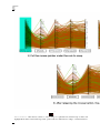
3.2.4.4.2. Scatter Plot
This layout can be used to see a correlation between 3 metrics (parameters). For example, if we have
a node with "usedMetric1" = 0, "usedMetric2" = 1 and, "usedMetric3" = 2, the node will be place in
the space with the coordinates : (0,1,2).
Following is an example, in which are 3 nodes. Those 3 nodes have 3 Metrics (called x,y,z). Node 1
equals to (0,0,0), Node 2 equals to (1,1,1) and Node 3 equals to (2,2,2).
We can see from the layout, that our correlation follow a linear function.
59
Functionalities
3.2.4.5. Force Directed
Force Directed layouts will try to place nodes so that, the distance in the graph (metric of the edges)
should be the closest to the distance on the drawing.
Warning !
: The previous property is not 100%.
3.2.4.5.1. Embedder (HDE)
The HDE layout, will only work on a 2D Mesh like graph. Algorithm documentation39
3.2.4.5.2. GEM (Frick)
The GEM layout, unlike the HDE layout, works on all graphs. But it can take a very long computing
time if the graph has more than 2000 nodes. Algorithm documentation40
3.2.4.6. Hierarchical
3.2.4.6.1. Hierarchical Graph
This layout, will place the nodes of a graph as if the graph was a tree. Algorithm documentation41
3.2.4.6.2. Hierarchical Graph 3D
This layout is the same that the "Hierarchical Graph" but in 3D. Algorithm documentation42
3.2.5. Size
3.2.5.1. Auto Sizing
39
40
41
42
../../doxygen/allPlugins.html#Embedder
../../doxygen/allPlugins.html#GEMLayout
../../doxygen/allPlugins.html#HierarchicalGraph
../../doxygen/allPlugins.html#GeneralGraph3D
60
Functionalities
The auto sizing algorithm will resize nodes and edges of a graph so that the graph gets easy to read.
The size of a node will depend on the number of its sons.
3.2.5.2. Fit to label
Fit to label, will resize nodes and edges so that labels fit in nodes.
3.2.5.3. Metric Mapping
The size of the nodes will change according to a metric.
3.2.6. General
3.2.6.1. Convolution
Convolution clustering is an approach to partitioning a graph that gives the user interactive control over
how many clusters to create. Tulip calculates a density function based on the chosen metric, displays
a convolution of its histogram, and partitions the graph according to the humps in the histogram.
3.2.6.2. Equal Value
This algorithm will create sub-graphs in which all nodes or all edges (not both at the same time), have
the same value. The ’Connected’ parameter indicates whether the subgraphs have to be connected or
not.
3.2.6.3. Hierarchical
This algorithm will divide the graph in 2 different subgraphs; the first one will contain nodes that
have the viewMetric value under than a certain limit, and, the other one, in which nodes will have a the
viewMetric value higher than the limit. Then, the algorithm will be re-applied to the subgraph (the one
with higher viewMetrics) until the subgraph contains less than 10 nodes. Algorithm documentation43
3.2.6.4. Quotient Clustering
This algorithm will create a metagraph. The metanodes will represent the subgraphs that already exist,
and a metaedge will be created between two metanodes if and only if it exist an edge whose source is
a node of a subgraph, and the target a node of an other subgraph.
Parameters :
• oriented : this parameter indicates whether the graph has to be considered as oriented or not. If it
is the case, two metaedges may exist between two metanodes One representing the edges from the nodes of
subgraph 1 to the nodes of subgraph 2, the second representing the edges from the nodes of subgraph 2 to the
nodes of subgraph 1.
• node function : this parameter enables to choose the function used to compute a measure value for
a meta-node using the values of its underlying nodes.
• edge function : this parameter enables to choose the function used to compute a measure value for
a meta-edge using the values of its underlying edges.
• meta-node label : this parameter enables to choose the string property used to compute the label
of the meta-nodes. An arbitrary underlying node is choosen and its associated value for the given property
becomes the meta-node label.This parameter enables to choose the string property to use when naming metenode.
43 ../../doxygen/allPlugins.html#HierarchicalClustering
61
Functionalities
• use name of subgraph : this parameter indicates whether the meta-node label has to be the same
as the name of the subgraph it represents. When checked, it superseeds the choice of the previous parameter.
• recursive : this parameter indicates whether the algorithm has to be applied along the entire
hierarchy of subgraphs.
• edge cardinality : this parameter indicates whether the cardinality of the underlying edges of the
meta-edges has to be computed or not. If yes, the property edgeCardinality will be created for the quotient
graph.
Algorithm documentation44
3.2.6.5. Strength Clustering
The strength clustering algorithm will recursively create subgraphs that are nested "small-worlds".
Wikipedia: small worlds.45
Algorithm documentation46
3.3. Properties of graph
In Tulip, there is a way to assign properties to each node or edge of the graph. Tulip defines two
kinds of property : intrinsic and extrinsic. The first represents the properties computed relatively to
the structure of graphs. But it is possible to assign values to the nodes or the edges that are not related
to the structure. For example, if we build the map of a region and the nodes represent the towns, the
label property can be used for the name of town. But it is not possible to determine the name with the
structure of the graph; this kind of property is extrinsic.
For each graph, Tulip provides a set of properties used by the renderer engine ; all begin with the
“view” prefix by convention : viewColor, viewLabel, viewLayout... They are updated during the
computation phase of the plugins. In the other hand, it is possible to define properties to store
informations relative to the graph. The number of this created properties are not limited.
3.3.1. Rendering Properties
Following is the list of rendering properties :
• viewBorderColor : Color of the border of an edge or a node.
• viewBorderWidth : Width of the border of an edge or a node.
• viewColor : color of an edge or a node.
• viewLabel : Label of an edge or a node.
• viewLabelColor : Color label of an edge or a node.
• viewLabelPosition : Label position (x,y,z) of an edge or a node.
• viewLayout : Position (x,y,z) of a node, or vector of the bends positions of the edges.
• viewMetric : Result value of the last measure ( Section 3.2.3, “Measure” ) algorithm applied.
• viewRotation : Rotation (0 to 360) of a node or an edge
44 ../../doxygen/allPlugins.html#QuotientClustering
45 http://en.wikipedia.org/wiki/Small-world_network
46 ../../doxygen/allPlugins.html#StrengthClustering
62
Functionalities
• viewSelection : Selection equals true if the node or edge is selected. False if it is not.
• viewShape : Shape of a node or a graph.
• viewSize : Size (height, width, depth) of a node or an edge. To re-size an edge, the parameter
"Size Interpolation" (CONTROL+R) must be switched off. For an edge, the three fields are : Width at source
of the edge, Width at the end of the edge, Size of the arrow.
• viewTexture : Texture will replace the color background of the node.
3.3.2. Using Properties
3.3.2.1. Updates of property values
As it is explained in the last section, it is possible to update the properties attached to the graph
elements with algorithms. An other solution is to update the values through the Property tab of the
Info Editor subwindow.
To give an example, create a graph :
• Select the property you want to update, viewSize in the local table, for example, to manage
the size of the nodes. Now, you can change all values or the value of one node.
1. Click on Set all, and write the new coordinates : (2.0, 2.0, 2.0)
2. Click on the line and the second column of the choosed node in the table. Change the values for the
width, the height and depth.
If you want to change properties of selected elements, use the check box selected only of the
Property tab.
• Select elements with the
mouse toolbar operation or using the ’Add/Remove Selection’ item displayed in the contextual pop-up menu
which appears when pressing on the mouse right button (press Ctrl key when mouse pressing on Mac).
• Select the property you want to modify : viewLabel.
• Click on the checkbox named Filter. The selected element just appears in the table above.
• Click on Set all and write the text you want to display : “Hey!”.
If you uncheck selected only, all nodes are in the table. It is possible to do the same thing with
the values of edges. You just have to click on the tab named Edges. There is an other solution to
modify the value of one node or edge :
• First select the
mouse toolbar operation, then click on the node or edge you want to update.
• The Element tab of the Info Editor subwindow is then selected. It displays the informations
of the element you clicked on.
63
Functionalities
3.3.2.2. Management of properties
The bottom of the Property subwindow enables to manage the properties. For each graph, as
explain before, a set of display properties already exists. If you want to create a new property :
• Click on the New button.
• Select the type of property, String. (other possibilities are Color, Integer, Layout, Metric, Size,
Selection)
• Type the name of the new Property (e.g. mylabel).
For removing a property, you just have to select the property and click on the button named Remove.
When deleting properties used by the render engine, those properties will be temporary removed from
the list but still continue to exist. Note that it is not possible to remove inherited properties.
The last feature is cloning property. Select the desired property and click on the button named Clone.
Type the name you have chosen. The new property keeps the values.
3.3.2.3. Find : make a request.
The find tool is in the Edit menu. Make a graph with several nodes. Change some properties of node
for making operations. Select nodes, check the Filter box and select the properties you want to
change : viewRotation. Click on the Set all button and type a value (20 for example). Now,
you have some node with a rotation of 0 degree and some other rotated of 20. So in the Find box :
• Select the property used for the request : viewRotation.
• Choose the operation and type a value for the comparaisons : = and 20, to find the element rotated
of 20 degrees.
• Select the action in the Options part : Add and the kind of the elements of the request : on
nodes.
3.4. Hierarchy
Tulip provides a system for the management of graphs hierarchies. The hierarchy sub-window
displays the existing instances of subgraphs or groups with their relationships, the user can change
the current view of the graph by clicking directly on the tree. When clicking the right mouse button,
a pop-up menu is displayed, it allows to manage the instances of cluster : remove, clone, create
subgraph.
3.4.1. Definitions :
3.4.1.1. Subgraphs :
A graph can have several parts of itself : these are stored in the subgraph instances. Some clustering
algorithms can made subgraphs. A subgraph share its elements with the graph, it is just a part of the
graph. It is possible to add properties for the subgraph only or to use the inherited properties.
For more information please visit : Wikipedia: Subgraphs 47
3.4.1.2. Groups :
47 http://en.wikipedia.org/wiki/Glossary_of_graph_theory#Subgraphs
64
Functionalities
Some graph can be a subgraph of an other graph. This kind of hierarchy enables to assign a graph to
a node.
3.4.1.3. Meta-graph :
A meta-graph is a graph that contains meta-nodes.
3.4.1.4. Meta-node :
A meta-node, is a node that contain a group. A meta node can contain / refer to the root graph (Fractal
effect).
3.4.1.5. Screen shots :
Following is an over view of a graph hierarchy :
The graph :
The subgraph and the meta-node :
The group :
65
Functionalities
3.4.2. Creating subgraphs or Groups :
3.4.2.1. Creating a subgraph :
To create a subgraph follow these steps :
• 1 . Select a few Nodes with the selection tool. (Shift + click, will add a node to the selection) To
select the edges that are between the selected nodes use the "Induced Sub-graph" algorithm.
• 2 . Create a subgraph : from the menu Edit->Create Subgraph, or from the keyboard,
Ctrl + Shift + G. Give it a name.
You will be able to find your new subgraph in the hierarchy onglet of the info editor window.
3.4.2.2. Creating a group :
To create a group follow these steps :
• 1 . Select a few Nodes with the selection tool. (Shift + click, will add a node to the selection) To
select the edges that are between the selected nodes use the "Induced Sub-graph" algorithm.
• 2 . Create a group : From the menu Edit->Create group, or from the keyboard Control
+ G. A warning saying "Grouping can not be done on the root graph a subgraph will be created" may pop up,
if it does, just click OK.
You will be able to find your new group in the hierarchy onglet of the info editor window.
Severals subgraphs will be created :
• A copy of the root graph called "groups" containing a meta-graph with a new meta-node pointing
to our group.
• A subgraph which is our new group.
66
Functionalities
3.4.3. Deleting / Ungrouping a subgraph or a Group :
3.4.3.1. Groups :
3.4.3.1.1. Delete .
To delete a group, left click on its name (in the Hierachy tab of Graph editor) => delete
By deleting a group, all nodes in this group will be deleted as well, whereas the meta-node will still
exist.
3.4.3.1.2. Ungroup .
To ungroup a group, select it, Left click => Ungroup
By ungrouping a group, all the layouts properties of the group’s nodes will be applied to the root
graph. The subgraphs created with the group wont be deleted.
3.4.3.2. Subgraphs :
To delete a subgraph, left click on its name (in the Info editor) => delete.
Deleting a subgraph has no effects on the root graph.
3.4.4. Using subgraphs or groups :
3.4.4.1. Subgraphs
3.4.4.1.1. Moving a node in a subgraph.
If you move a node in a subgraph, the same node will be moved in the root graph.
3.4.4.1.2. Using an algorithm on a subgraph
If you use a layout algorithm on a subgraph, all changed layout properties will be applied to the root
graph.
If you use a Measure algorithm on a subgraph, New local properties will be created. Those properties
wont be applied to the root graphs.
3.4.4.2. Groups :
Changes on groups, wont be applied to the root graph unless you ungroup the group.
3.4.5. Algorithms that creates subgraphs :
You can find those algorithms in the menu Algorithm => General.
• Equal Value.Section 3.2.6.2, “Equal Value”
• Hierarchical.Section 3.2.6.3, “Hierarchical”
• Quotient Clustering.Section 3.2.6.4, “Quotient Clustering”
• Strength Clustering.Section 3.2.6.5, “Strength Clustering”
67
Functionalities
3.5. Statistics Panel (not available in standard
version)
Tulip also provides a simple statistics interface which allows the user to compute Histograms, Scatter
Plots, Augmented Displays and Clustering. The computation of Histogram and Scatter Plot depends
on a number for metrics, chosen by the user (from 1 to 3), and a discretization step (one given per
metric). Finally, the clustering is performed from a clustering plane, specified by the user with a plane
equation.
3.6. Text Rendering
It is possible to assign a label to each element of the graph. Tulip can display them with three methods
: 3D and texture for node labels, bitmap for node and edge labels.
Figure 3.1. Bitmap Rendering
Figure 3.2. 3D Rendering
68
Functionalities
Figure 3.3. Texture Rendering
In a future version of Tulip, It will be possible to create labels with XML tags like the HTML
rendering. Some tags will be available in order to allow the user to organize the content of the labels.
69
Chapter 4. Plugins Management
To open plugins management click on Plugins in Help menu.
4.1. Interface
Main window :
The main window is divided in two sides :
• Left side : Plugins list view
• Right side : Documentation
70
Plugins
Management
4.1.1. Plugins List
The "Installed" group displays the locally installed plugins. The others group displays the plugins
available on server.
At the version level you can see the status of the plugin : nothing, version or installed.
• Nothing : Plugin is not installed.
• Version number : Plugin is installed, the version number you can see is the locally installed
version.
• Installed : Plugin is installed and its version is the same on the server.
4.1.2. Plugin’s Documentation
If you want to see the plugin’s documentation, click on the version number of a plugin (not on the
checkbox : this is to install/remove plugin).
Documentation is composed in two groups :
• On the top : brief description of the plugin (version, author, info ...)
• At the bottom : detailed description of the plugin.
4.2. Setup
To setup plugins manager click on Configure->Servers button of menu.
Servers configuration :
4.2.1. Add a server
To add a server, click on Add Server button. After that you have a window to enter the server
address.
71
Plugins
Management
And example of server address is : "http://tulip.labri.fr/pluginsServer/server.php".
4.2.2. Modify/Remove a server
To modify a server : select it then click on Modify button. After that you can change the server
address. The server name cannot be changed because it is managed by the server.
To remove a server : select it then click on Remove button.
4.3. Install/Remove plugins
4.3.1. Simple installation
If you want to install a plugin, just click on the check box at the version level.
After that click on Apply Change in File menu. A new window appears :
72
Plugins
Management
When all plugins are installed/removed you can click on Ok button.
After plugin installation/remove you have to restart tulip to see the modification.
4.3.2. Installation/Remove with dependencies
At installation, if the plugin depends on other plugins a new window appears with the list of needed
plugins. If you click on Yes, the needed plugins will be installed too. If you click on No, the needed
plugins won’t be installed.
When you remove plugin, this is alike with plugins needing the one you want to remove.
73
Chapter 5. Tutorials
5.1. First Step
In this part, the goal is to help you to simply make a graph and to save your work.
5.1.1. First graph display
5.1.1.1. Importation of a graph
• Select the File->Import item.
• Select a method of importation : Grid approximation, for example.
Do not modify the default parameters. Here is displayed the graph with nodes (red) and edges (black).
With the wheel of the mouse, you can zoom on the graph to see a specific node. In moving the mouse
with its left button pressed, you can translate the graph in the plane of the view, pressing the key
SHIFT for rotation and the key Ctrl (Alt key on Mac) to rotate around the z axis and zoom. In order
to come back to the oldest view, Select View->Center view from the menu bar.
• Select Algorithm->Measure->Misc->Id from the menu bar, to compute a value (metric)
for each node and edge of the graph.
The graph is now displayed with colors depending of the metric. You can change the colors with
the menu : Algorithm->Color->Metric Mapping. This plugin computes an interpolation
between the two selected colors.
5.1.1.2. Creation of a graph
In this section, we learn how to create its own graph, element by element.
• Select the File->New from the menu bar to create a new graph.
• Create a graph adding nodes and edges. For a node, select the
mouse toolbar operation and click on the position you have chosen. To insert an edge, select the
mouse toolbar operation. Click on the source node, then on the target node. You can display or hide them
with Edges checkbox in the Overview subwindow. In the same way, you can display or hide the arrows
checking Arrows.
• Delete elements of the graph. Select the
mouse toolbar operation, then click on the element you want to delete.
74
Tutorials
5.1.2. Save options
To save your work, you just have to select File->Save or Save as: a dialog appears allowing to
enter the author of the graph and some comments; then after clicking on the ’OK’ button, just type the
file name and choose its location.
The second way to make a save is to export the graph in a special format : GML or TLP (equivalent
to Save as). Select File->Export and the format of your choice, then choose the file name and
location.
5.1.3. Algorithms
This part explains how to apply an algorithm to a graph. Previously, you have created
or imported a graph.
Select Algorithm->Layout (for example) and an algorithm :
Hierarchical->Hierarchical Graph for example.
In this case, we use an algorithm dealing with the layout of the nodes and the edges. It is possible to
apply all other kinds of algorithm. Some layout algorithms may not apply to your graph if it does
not belong to the right category of graphs. With the Bubble Tree layout, you can not display a
grid. If it is not valid, a pop-up message will displayed explaining the problem.
5.2. Improving a layout
5.2.1. Introduction
In this tutorial, we will show you how to use, layouts algorithms, and graph properties to obtain a nice
an clear graph. To do so, we will first import a file-system structure, and then use the graph properties
to find specific files. (*.cpp or *.hpp ...)
5.2.2. File-system importation
To import a file-system we need to select the File System Directory importation tool which
is in the menu File->Import->Misc.
A "file browser dialog" will pop-up to select the root directory that you want. On this dialog, you just
need to select a directory for instance, your documents (On Windows : My Documents).
The importation plug in will work for some time, and a tree graph will appear representing the file
system chosen.
75
Tutorials
To follow the rest of this tutorial you need to download this tulip graph file : Graph1 . Load this
compressed tulip file into the software (File->Open).
5.2.3. Using other Layouts :
5.2.3.1. Bubble Tree Layout :
This layout algorithm can be found in the menu Algorithm->Layout->Tree. The bubble tree
layout is very useful to notice directories that have the same structure. In this section, we will try to
locate those directories.
To have a better view on the tree, we will create a new NodeLinkDiagramComponent. Menu : View>NodeLinkDiagramComponent. When the new view is created, we need to re-organize the windows.
Menu : Windows->Tile.
Now that we can see the both views at the same time, we will zoom in (right window). Select the
magnifying glass tool, and draw a bounding box on the left side of the graph. Just like this :
1 http://www.labri.fr/perso/auber/projects/tulip/samples/filesystem.tlp.gz
76
Tutorials
As you can see, two nodes looks very alike. By using the "Get Information " tool, we can get there
ids : Node 1965 and node 2009. Indeed, those to directories have the same structure since they both
contains plug-ins source files.
We will now re-center the view (View->Center View or Ctrl+Shift+C).
Let’s say that we now want to study our graph without the plug-in directory. To delete it we have first
to select it, and then select all its sub directories.
• Select the plug-in directory : Use the Find tool, (Edit->Find or Ctrl+F) with the field Input
property set to "name", filter function set to "=" and filter value set to "plugins".
• Select all its sub-directories :
Use the Algorithm->Selection->Reachable
Sub-Graph algorithm with the field distance set to 50.
• Delete all the selection : press Del
• Re-draw the bubble layout Algorithm->Layout->Tree->Bubble Tree.
Following is what you should see :
77
Tutorials
As you can see, the bubble tree layout can be quite useful.
5.2.3.2. The Tree Map layout :
This Layout algorithm can be found in the menu Algorithm->Layout->Tree. The treemap
layout is very useful to notice large disk usage files. This section will show you how to use the tree
map layout
First, make sure that you have unchecked the Force Ratio option that you can access via the menu
Options.
Apply the layout algorithm Algorithm->Layout->Tree->Squarified Tree Map with
the following parameters :
• Metric : set to "size".
• Aspect Ratio : set to 1
• Texture? : checked
Do not forget to refresh the views (Ctrl+Shift+R). Following is what you should see :
As you can see, we easily get a global information on the size of files. Which is the biggest, or, which
is the smallest ? But, we can also see the structure of directories, since files and directories are nested
nodes. See Wikipedia : Tree Maps 2 for more information.
5.2.3.3. Improved Walker layout :
This layout can be find in the Algorithm->Layout->Tree->Improve Walker.
Use the following parameters :
• Node Size : viewSize
• Orientation : Left to right.
2 http://en.wikipedia.org/wiki/Tree_map
78
Tutorials
• Orthogonal : Checked.
• Layer Spacing : Default value.
• Node Spacing : Default Value.
You should see a tree looking like this :
As you can see, the improve walker layout, is just a hierarchical layout. It is very useful to understand
the tree structure of a file system.
5.2.4. Showing Labels
First, right click on the view and select Dialog->Rendering parameters. In the Rendering
Parameters dialog go in Layers tab and check the Nodes Label visibles box
We will now try to add labels to the nodes. To do so, select the node property called "name" in the
info editor window, click on the button To Labels.
You should now see a graph looking like that :
79
Tutorials
As you can see, the labels, don’t fit in nodes and it is very hard to read the graph. To fix this problem
go on rendering parameters dialog and in the Labels box, the field Type must be equal to "3D". Then,
apply the Algorithm->Size->Fit To Label algorithm.
You should obtain something like this.
80
Tutorials
By zooming in we can see the labels :
If you want to display the big file (high disc space) with big nodes, use the
Algorithm->Size->Metric Mapping algorithm with the parameter called "property"
set to "size".
5.2.5. Showing a specific kind of file.
Now that our graph as a nice and clear layout, we would like to locate all of our Source files (*.cpp).
To do so, we will use the Find tool (Edit->Find or Ctrl+F).
Use the following parameters :
• Input Property : name
• Filter : filter function set to "=" and filter value set to ".*cpp or .*hpp". For more details on regular
expressions, follow this link : WikiPedia : Regex 3
• Options : check the Replace radio button and select On nodes.
Now that our source files are selected, we will apply a different color to them.
In the info editor window, select the node property called "viewColor", check the selected only
option. Now that we only see the "viewColor" property of the selected nodes, click on the button Set
all and choose the color that you want. (We choosed green)
You should see a graph like the one following :
3 http://en.wikipedia.org/wiki/Regular_expression
81
Tutorials
5.2.6. Conclusion
As you could have seen, tulip implements powerful layouts and tools, to make a simple and
understandable graph from a complex one.
82
Tutorials
5.3. People in InfoVis
5.3.1. Analyzing an author.
Before anything, download, and open this tulip graph file4 . Click on the tab Hierarchy (in the info
editor window) and select the subgraph GRCite. You need to delete the other sub graphs by doing a
right click on there name, and then "remove".
This graph represent the relations between authors, conferences and papers. To distinguish paper,
conferences and authors, we will re-color them :
• Select all papers : Press on Ctrl+F to display the find tool. In the Input Property field, select the
property "type". And on the line below, set the filter function to "=" and the filter value to 0, before clicking
on the Find button.
• Re-color the nodes in red : Select the tab Property (in the info editor). Check the "selected only"
option. Select the property viewColor, and, by clicking on the button "Set all" choose the red color.
Repeat the actions above, for authors (type = 2 ) and conferences (type = 1) with other color (blue ,
yellow).
You should obtain something like this :
4 http://tulip.labri.fr/samples/GRCite.tlp.gz
83
Tutorials
Select an author :
Let’s pick a single author to investigate, in this case George Robertson. First, we interactively select
that node by hitting Ctrl+F for the find tool, choosing the "titleshort" property, the "=" as filter
fuction, and the regular expression "G.*Rob.*" as filter value. We then quickly check to see how
he is connected to the entire graph by temporarily moving that node away from the others to see
roughly how many edges are attached to it.
Following is what you should get :
Go deeper :
We then select the menu item Algorithm->Selection->Reachable Sub-Graph,
type 1 for the distance into the popup panel and 0 for the direction of the edges (outgoing).
We then select the menu item Edit->Create Subgraph to save this selection for
further manipulation, naming it GR.1hop.outgoing.
We then select this new subgraph
in the hierarchy tab, and lay out this subgraph using a hierarchical drawing algorithm
(Algorithm->Layout->Hierarchical->Hierarchical graph).
We can see simply from the drawing which papers were published first, as they are cited by the later
ones. Robertson has published 11 papers in this database. The coloring by the number of citations
(Algorithm->Color->Metric Mapping, with field property set to "arityOut" ) shows that
"Cone Trees" is his most influential work.
84
Tutorials
Finally, we select all papers by hitting Ctrl+F for the find tool, choosing the type property, the "="
filter, and the value 0 for papers. We explicitly add Robertson to the selection using the selection tool
to select its edges too (see below), and save this whole set to a new subgraph that we name GRCitesub:
85
Tutorials
In the new subgraph, we then select the Robertson node.
Again as above, use the
Algorithm->Selection->Reachable Sub-Graph algorithm, pick a depth of 2
to find all papers that cite a paper written by Robertson, and save the resulting subgraph
using the Edit->Create Subgraph menu.
The final image shows the result of using the
Algorithm->Layout->Hierarchical Graph layout.
86
Tutorials
You can now close this graph since we are going to use an other one for the following of this tutorial.
The next graph is similar to the this one but, has coauthorship edges linking authors who write papers
together. You can download it5 and open it in tulip.
5.3.2. What, if any, are the relationships between two or
more or all researchers
5.3.2.1. Focusing on Two Authors
Here we focus on the relationship between two authors, in this case Robertson and Card.
To select them use the find tool, with, at the first time the regular expressions : "G.*Rob.*". And at a
second time, the regular expression ".*Card.*" and the "add" option checked. To move those selected
nodes away from the main layout, use the "moving selection" tool. If you click on one of the node,
you will be able to move both nodes at the same time.
5 http://tulip.labri.fr/samples/GRSC.tlp.gz
87
Tutorials
Select Card and Roberts at the same time ( Press Shift while clicking on a node). Select all their
neighbors by applying the Algorithm->Selection->Reachable Sub-Graph algorithm
with distance 1. Create a new Subgraph.
Following is a hierarchical layout of the neighborhood of all outgoing edges one hop away; that is, the
publications and coauthors of the union of Card and Robertson.
You can repeat those operations for Robertson only and Card only :
88
Tutorials
The similarity of these final three images shows the very strong ties between these two authors.
You can now close this graph since we are going to use an other one for the following of this tutorial.
The next graph is similar to the old one but, has links between author and conference by following
links from author to paper, and from paper to conference. Then, delete papers. You can download it6
and open it in tulip.
5.3.2.2. Central Authors and Conferences: Overview
To show the large-scale structure of this dataset, we colored Authors in green and conferences in
blue with a GEM layout (Algorithm->Layout->Force Directed->GEM). We deleted all
the papers nodes.
By zooming in :
6 http://tulip.labri.fr/samples/ConfAuth.tlp.gz
89
Tutorials
We select only the large connected component (the big set of nodes) : Select a fiew nodes in the center
of the component and run the "Reachable Subgraph" selection algorithm with distance set to 50.
Color the authors by the Strahler metric: Run the Algorithm->Measure->Graph->Strahler
algorithm and then a Algorithm->Color->Metric Mapping algorithm.
Finally, we color papers in white.
This layout, shows the branching structure of the dataset.
90
Tutorials
To distinguish authors and conferences :
Select all authors (nodes of type 2) and set their viewLabelColor property to red.
91
Tutorials
5.3.2.3. Central Authors and Conferences: Top Conferences
It is very simple to see top conferences since they are the ones where the number of authors is high.
The Metric Degree will help us to highlight them (Algorithm->Measure->Graph->Degree
).
92
Tutorials
5.3.2.4. Central Authors and Conferences: Top Authors
Run the Algorithm->Measure->Graph->Strahler algorithm to see strong ties between
conferences and authors :
Then run the Algorithm->General->Convolution, the value of the "discretization" parameter should be near 30 to obtain 5 clusters ) (Picture 1) to obtain the following clusters (Picture 2):
93
Tutorials
The Strahler-Convolution clustering yields five clusters, according to increasing centrality. The first
cluster is mostly yellow, and contains most of the data. The second cluster contains a next tier of
94
Tutorials
26 authors that have had a relatively strong impact. The third cluster contains a group of 7 influential
authors (Chi, Bederson, Eick, Rao, Pirolli, Ward, and Brown), and the fourth cluster (Roth, Robertson,
Keim, and Stasko) is yet more central. The fifth cluster is the single node of Mackinlay, and the last
one is Card and Shneiderman. Our automatic clustering method clearly yields very believeable results
in this case.
In the last section, we will use an other graph. Please download it7 and open it in tulip.
5.3.2.5. Hierarchical Structure of Interauthor Connections
To be able to see the labels within metanode check the "metanode label" visible box in the Layers tab
in Rendering Parameters dialog.
The clusters have been computed using the Algorithm->General->Strength clustering algorithm.
The overview image from the previous section, showing the graph of all authors and papers, is
extremely cluttered. In the previous task we show one way to extricate more information, by finding
the most important items via convolution clustering. Another clustering approach, small-worlds
clustering, allows us to instead navigate through a hierarchical subdivision of the entire dataset. The
simplified overview allows us to understand the graph’s high level structure. The strength metric
computes the number of cycles of length 3 and 4 passing through each edge, normalized by the
maximum possible value. The first image shows the clustered dataset. Small-world navigation is
useful when exploring an unfamiliar graph to quickly find the structure of complex components.
The eccentricity metric (Algorithm->Measure->Graph->Eccentricity), which measures
whether nodes are peripheral (here in yellow) or central (here in blue), guides us to complexity
immediately. This metric is O(n^3), but the small-world decomposition simplifies the graph, making
the computation tractable.
7 http://tulip.labri.fr/samples/ConfAuthRecSmallWorld.tlp.gz
95
Tutorials
The picture shows zooming in towards the node that has many blue lines leading to it.
We then jump inside that cluster (Select the metanode, Right Click, Go inside), which is itself a smallworld graph.
96
Tutorials
We once again zoom towards the most central node with many blue edges, where we see a cluster that
has the InfoVis 96 conference and all the authors who only published the infovis community in that
year.
We see this star shape small-world decomposition only for the InfoVis symposia, because of the nature
of this dataset: it is only the InfoVis symposia that have a complete set of authors and papers available.
5.4. Statistics Panel (not available in the downloadable binary versions, requires configuration with --enable-stats-gui when compiling
Tulip from source code)
5.4.1. Introduction
97
Tutorials
This section will explain how to use the statistics panel in Tulip. The tutorial is composed of 3 main
parts. Firstly, you will see how to generate a scatter plot or an histogram from a graph. In a second
part, you will see how to enable augmented displays on the graph. And finally, you will see how to
clusterize the graph from the statistics values previously computed.
Every screenshots that will be shown in this tutorial are based on this tree :
Figure 5.1. Statistics base test set : a tree
5.4.2. Scatter plot and Histogram computation
The first thing to understand about the statistics panel is how to generate an histogram or a scatter plot
from the graph. The computation of histogram/scatter plot is based on metrics. So, in a first time, you
will have to compute metrics. In the example, we have computed three metrics : Arity, DAGLevel and
Depth. The new metrics are automatically updated on the Available Metrics list on the Stats panel :
Figure 5.2. The metrics available in the statistics panel
98
Tutorials
Now that you have some metrics available. You can add them to the Used Metrics list simply using
the Add and Remove buttons. The number of dimensions of the result will only depend of the numbers
of metrics you add to the list. With only one metric added, you will have an frequency histogram
displayed. With two (resp three) metrics you will have a 2D (resp. 3D) scatter plot. Each metric
representing a different dimension.
In the example, we have only added the DAGLevel metric to the Used Metrics list :
Figure 5.3. A single metric for an histogram
99
Tutorials
As you can see, adding a metric implies some changes in the interface. The bottom button becomes
enabled, so as the edit box corresponding to Discretization Step 1. You can specify a discretization
step, even if it is not really useful for our example.
Now the last step before having a beautiful frequency histogram displayed : asking the panel to
compute it. Just click on the Compute Histogram button. That’s it !!! You have your first histogram :
congratulations !!!
Figure 5.4. Your first histogram
100
Tutorials
Now that we have an histogram. We are not going to stop here. Let’s generate a scatter plot in three
dimensions. Just add two other metrics to the Used Metrics list. You will notice that the text of the
Compute Histogram button now becomes Compute Scatter Plot. Just click it and you will have a
scatter plot.
Here is the result with our base tree and the three metrics mentionned in the introduction :
Figure 5.5. Scatter plot generated from the three metrics
101
Tutorials
As a conclusion to this first part, you have learnt how to generate a simple frequency histogram from
a graph and a metric. You have also learnt how to generate a whole scatter plot from 2 to 3 metrics. In
the next part, you will learn how to display the basic statical values on the graph.
5.4.3. Statistics values and Augmented displays
Now, we will see how to compute the main statistics results, and how to display them on the generated
Histogram/Scatter Plot. Switch to the Display tab of the statistics panel. Yet, everything is grayed. To
compute the values of the tab, you must click on the bottom button Compute Results. Note that this
button is reachable on every tab on the panel but you will be able to click it only if the Used Metrics
list of the Computation tab is not empty.
Figure 5.6. Click on the button Compute Result to enable the tab
102
Tutorials
Once the results computed, most of the elements of the panel should be enabled. Note that the
Regression Function group is enabled only if you hase two metrics in the Used Metrics list, and
Eigenvectors is enabled only if you have three metrics in the Used Metrics list.
The checkboxes next to each groupboxes (except the Variance one) are used to display on the
Histogram/Scatter plot, the result of the group. For example : checking the checkbox next to Average
will display the average point on the graph (an Axis Point in red (c.f. GlAugmentedDisplay in the
developer handbook)).
Figure 5.7. Checking Average on the display tab
103
Tutorials
Figure 5.8. The average of the scatter plot
104
Tutorials
Every augmented display works the same way. You will just have to click on the checkbox next to
the group to enable the display of the result. Note that you can’t display the Variance since this result
can’t be represented in an interesting way on the graph. use instead the standard deviation.
Now that you know how to display the statistics results, you will see how to clusterize the scatter plot
/ histogram from these values.
5.4.4. Clustering with the statistics panel
The last part of this tutorial will teach you how to clusterize from the statistics results previously
computed. Firstly, switch to the Clustering tab. The Combobox Clustering Value lists the available
start for a clustering plane depending on what has been computed before. Select Average (Z)(you must
have selected 3 metrics), the plane coordinates will be modified according to the values of the average’s
Z coordinate. Check the Display Clustering Plane checkbox. The plane appears in transparent red,
showing you the future two clusters.
Figure 5.9. Selection of the clustering value
105
Tutorials
Figure 5.10. The clustering plane
106
Tutorials
In order to have the good clustering, you can modify the plane equation to move the plane. Finally,
to clusterize, just click on the Clusterize button. That’s it ! The graph is now clusterized. In order to
ensure, just check the Cluster Tree.
Figure 5.11. The new clusters after statistic clustering
107
Tutorials
5.4.5. Conclusion
As a conclusion, you have learnt how to use the statistics panel of Tulip. As you can see, obtaining
results is easy and fast. If you have any question about that panel, you can contact it’s creator at
<[email protected]>
108