1
USB Data Logger User Manual
This User Manual refers to the Software/Firmware Version 9.90. Other versions may differ in
some details.
By Mauro Grassi.
Tips: A note on the Installation of the Windows PC Host Software
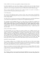
As an addendum to the instructions given in the original series of articles in SILICON CHIP
(December 2010, January, February 2011), the PC Host uses the Windows default programs to open
files to display them, the default program depends on the extension of the file. The most common
extensions used by the PC host are “.txt” (the default program is usually NotePad, but this can be
overridden). The next most common file extension used by the PC Host is “.bin”, indicating a
binary file. Windows OSs will not usually be setup to automatically display this type of file.
Therefore, we recommend installing the freeware binary file viewer: “XVI32”, which can be
downloaded
from
the
following
website:
http://www.chmaas.handshake.de/delphi/freeware/xvi32/xvi32.htm”
In this document we give the correct syntax for all the built in global functions and global variables,
as well as the define constants. We also give a description of the scripting language used.
The global functions and global variables are given in alphabetical order.
Scripting Language Commands
Variables are Local or Global, so are Functions. Local variables/functions have scope only within
the script, on the other hand, global variables/functions have scope for all scripts. Note however that
the same global variable, accessed from different scripts, may still access different physical
memory. For example, while the $$return global variable is common to all scripts, this is not true
for the $$vm global function, which accesses the virtual machine associated with the script.
Global function names begin with two '@' characters, local function names begin with one '@'
character. Similarly, global variable names begin with two '$' characters, while local variable names
begin with one '$' character.
Numeric Constants
The scripting language natively recognises numeric constants in one of the following formats:
Decimal Integer: an integer specified base 10 is simply a string made up of a finite number of
decimal digits in the range from 0-9 (inclusive). For eg, 192.
Hexadecimal Integer: an integer specified base 16 is a string made up of the constants “0x”
followed by a string made up a finite number of hexadecimal digits in the range 0-9 and A-F or a-f.
For eg, 0xA8.
Binary Integer: an integer specified base 2 is a string made up of the constants “0b” followed by a
string made up a finite number of binary digits in the range 0-1. For eg, 0b1101.
Floating Point Number: a 32 bit floating point number, for eg. -1.34.
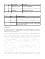
Built In Commands (reserved keywords)
The following built in keywords are part of the scripting language. Note that the syntax is specified
as follows. Necessary parameters are enclosed in '<' and '>' brackets, while optional parameters are
enclosed in '[' and ']' brackets (both are shown in italics).
SCRIPT/script: this keyword (together with the HEADER/header keyword) is used to declare a
script. It is followed by the name of the script and the body of the script, which is enclosed in curly
brackets. The syntax is: script <script name> { <script body> }
SLEEP/sleep: suspends execution of this script for the specified number of seconds. The syntax is:
sleep(<number of seconds>);. For eg, sleep(10); suspends execution for 10 seconds.
SLEEPUNTIL/sleepUntil: suspends execution of this script until an absolute time in the future.
The syntax is: sleepUntil([year]:[month]:[day]:[hour]:[minute]:<second>); For eg,
sleepUntil(1:13:23:24); will suspend execution until the day of the month equals 1 and the time is
13:23:24. You can omit all the arguments except the seconds.
TIMEUNTIL/timeUntil: returns the number of seconds until the nearest absolute time in the
future that matches the argument. The syntax is: timeUntil([month]:[day]:[hour]:
[minute]:<second>); For eg, timeUntil(10); will return the number of seconds until the next
absolute time when the seconds equal 10.
TIME/time: loads the script's time register with a specific time. The syntax is: time([month]:
[day]:[hour]:[minute]:<second>);
PRECISION/precision: sets the number of decimal places to display when printing the value of a
floating point variable. The default is 0, the syntax is: precision(<num>); where <num> is the
number of decimal places.
NEWLINE/newline: used as an argument to the PRINT/print command to print a newline.
PF/pf: print function command is used as an argument to the PRINT/print command to print a
specific type of data. The syntax is: pf(<function>); where function is one of a number of defined
constants.
IF/if: used to conditionally execute a block of code. The syntax is: if(<conditional>){ <block> };
The block of code <block> is executed only if <conditional> is non zero. If <block> consists of a
single statement, the curly brackets can be omitted but a semi colon must terminate the statement.
ELSE/else: can be used with the IF/if command to conditionally execute two blocks of code. The
syntax is: if(<conditional>){ <block 1> }; else { <block 2> }; The block of code <block 1> is
executed only if <conditional> is non zero, otherwise <block 2> is executed. If <block 1> consists
of a single statement, the curly brackets can be omitted (same applies for block 2), but a semi colon
must terminate the statement.
HEADER/header: keyword used to define the header of a script. The syntax is: header <name> {
<header code> } Every script must have a header defined by the header keyword, but the header
code body can be empty.
PRINT/print: this command takes a comma separated list of arguments and prints out their values
to the scripts log file (or open pipes). The syntax is: print <arg 1>, <arg 2> … <arg N>; where each
argument can be any expression, or a print function command, or a newline command.
OPENPIPES/openPipes: this command is used to open a number of pipes for the script. The
script's output (through the print command) is then sent to all open pipes. The syntax is
openPipes(<pipes>); where the value <pipes> is a logical OR of all the pipes to open. The pipe
codes are defined as define constants.
CLOSEPIPES/closePipes: this command is used to close a number of pipes for the script. The
script's output (through the print command) is sent to all open pipes. The syntax is:
closePipes(<pipes>); where the value <pipes> is a logical OR of all the pipes to open. The pipe
codes are defined as define constants.
CLEARFILE/clearFile: this command is used to define a new log file for the script. The argument
is a comma separated list of arguments (as in the print command) that will form the file name for
the new log file for the script. If a file of that name already exists, it will be deleted. The syntax is:
clearFile <arg 1>, <arg 2>, … <arg N>; where each argument is as for the print command.
RESET/reset: this command simply resets the current script to begin execution anew. The syntax is
reset;
OPENFILE/openFile: this command is used to define a new log file for the script. The argument is
a comma separated list of arguments (as in the print command) that will form the file name for the
log file for the script. If a file of that name already exists, it will be appended to. The syntax is:
openFile <arg 1>, <arg 2>, … <arg N>; where each argument is as for the print command.
SERIAL/serial: this command is the same as the PRINT/print command, except the output is sent
only to the serial port pipe for the script (rather than to all open pipes).
NMEA/nmea: this command is the same as the SERIAL/serial command, except each character of
the output is added to a running transmit CRC (by repeatedly XORing the value) (the global
variable $$serial.TxCRC holds the CRC). The CRC can then be displayed at the end of the line
using the pf(#nmea) print function to add the CRC sequence at the end of the NMEA command.
This is useful for interfacing to NMEA compliant devices, such as a GPS module.
MATCHNMEA/matchNMEA: this command takes as argument a comma separated list consisting
of a match string for matching incoming NMEA packets on the serial port. On a match, the input is
processed. The string is made up of the following commands:
's' + literal string :match the literal string exactly (comma marks the end and can't be matched in the
string, use the 'c' option to match the comma)
'c' + char
: match the character exactly...
'$'
: match any character & store it...
'@'
: match any character but do not store the result...
'd' + n (n:1-9) : match up to n decimal digits and store the output...
'x' + n (n:1-9) : match up to n hex digits and store the output...
'\0'
: end the command string...
'f'
:
match a floating point number...
For example, the command matchNMEA “sGPRMC,d2d2f,cA,d2f,$,d3f,$,f,f,d2d2d2”; can be
used to match NMEA sentences from a GPS module in the format GPRMC.
FUNCTION/function: this keyword is used to define a local function. It can then be called from
anywhere in the code to implement procedural abstraction. The syntax is: function
<functionname>(<num>){ <block> } The <functionname> must start with a single '@' character.
<num> holds the number of arguments to the function. Each argument can then be referred to in the
code block <block> by using the expression $<n> where <n> is the nth argument passed. For
example, $2 refers to the second argument passed.
DECIMAL/decimal: this command can be used in a comma separated argument (to the print
command and other commands using the same comma separated argument list) to override the
default printing of a number (set by the precision command). This command forces the display to
be a decimal number with the indicated number of decimal points. The syntax is decimal(<value>,
<num>); where <value> is the value and <num> is the number of decimal places.
BASE/base: this command can be used in a comma separated argument (to the print command and
other commands using the same comma separated argument list) to override the default printing of
a number. This command forces the display to be an integer relative to the indicated base. The
syntax is base(<value>, <base>, <numdigits>); where <value> is the value and <base> is the base
and <numdigits> is the number of digits to print (the <numdigits> argument can be omitted). For
example, base(10, 16); will print 'A' (the hexadecimal code for 10).
CHAR/char: this command can be used in a comma separated argument (to the print command and
other commands using the same comma separated argument list) to print the ASCII character
corresponding to the argument. The syntax is char(<value>); For example, char(0x41); will print
'A'.
WHILE/while: this command is used to execute a command block as long as a condition holds.
The syntax is: while(<conditional>){ <block> } The block of code is executed as long as the
conditional is non zero. If <block> is a single command, the curly brackets can be omitted (but a
semi colon must terminate the statement).
AND/and: used to combine two conditional statements to form a compound statement that is true
precisely when both are true.
XOR/xor: used to combine two conditional statements to form a compound statement that is true
when exactly one is true.
OR/or: used to combine two conditional statements to form a compound statement that is true
when at least one is true.
Operators
The following operators can be used in a conditional statement, or in an arithmetic expression:
Operator Function
Example
'+'
Addition
$A=45+54; ($A then equals 99)
'-'
Subtraction
$A=10-1; ($A then equals 9)
'*'
Multiplication $A=2*8; ($A then equals 16)
'/'
Division
$A=4/5; ($A then equals 0.8)
'^'
Exponent
$A=2^3; ($A then equals 8)
'%'
Modulo
$A=16 % 5; ($A then equals 1)
'=='
Equality
$A==12 (the result is non zero if $A is equal to 12, 0 otherwise)
'!='
Non Equality
$A!=12 (the result is non zero if $A is not equal to 12, 0 otherwise)
'>='
Greater than or $A>=12 (the result is non zero if $A is greater than or equal to 12, 0
equal to
otherwise)
'<='
Less than or $A<=12 (the result is non zero if $A is less than or equal to 12, 0
equal to
otherwise)
'>'
Greater than
$A>12 (the result is non zero if $A is greater than 12, 0 otherwise)
'<'
Less than
$A<12 (the result is non zero if $A is less than 12, 0 otherwise)
&
Address of
This operator returns the address of a variable.
#
Size of
This operator returns the size of a variable.
'='
Assignment
$A=23; (Assign the value 23 to variable $A)
Local Variables & Global Variables
Local variables' names begin with a single '$' character, followed by a letter and then any number of
letters and numbers. Global variables' names begin with two '$' characters. Note that arguments to
local functions are specified with a single '$' character followed by a decimal number (indicated the
place in the argument list, for example $1 specifies the first argument passed to the local function,
etc.).
Local String Variables & Global String Variables
Local string variables' names begin with a single '*' character, followed by a letter and then any
number of letters and numbers. Global variables' names begin with two '**' characters.
Local Functions & Global Functions
Local functions' names begin with a single '@' character, while global functions' names begin with
two '@' characters. There are many defined global functions for controlling many aspects of the
data logger. See below for a number of example scripts that show how to use the built in commands.
Define Constants
Define constants can be redefined at compile time, but the compiler will issue a warning if this is
the case (note that warnings are not shown unless the Verbose check box is checked). Define
constants' names begin with a single '#' character. The following define constants are built in (note
in particular, the defined constants which are PRINT FUNCTION arguments, which allow you to
log important information along with your data, including the time:
Syntax:
Value :
Effect:
#A0
0, 0x00
analog channel A0 (multiplexed with digital channel D4)
Syntax:
Value :
Effect:
#A1
1, 0x01
analog channel A1 (multiplexed with digital channel D5)
Syntax:
Value :
Effect:
#A2
2, 0x02
analog channel A2
Syntax:
Value :
Effect:
#A3
3, 0x03
analog channel A3
Syntax:
Value :
Effect:
#D0
0, 0x00
digital channel D0
Syntax:
Value :
Effect:
#D1
1, 0x01
digital channel D1
Syntax:
Value :
Effect:
#D2
2, 0x02
digital channel D2
Syntax:
Value :
Effect:
#D3
3, 0x03
digital channel D3
Syntax:
Value :
Effect:
#D4
4, 0x04
digital channel D4 (multiplexed with analog channel A0)
Syntax:
Value :
Effect:
#D5
5, 0x05
digital channel D5 (multiplexed with analog channel A1)
Syntax:
Value :
Effect:
#defaultExecMode
0, 0x00
use the system default execution mode (restart on HALT)
Syntax:
Value :
Effect:
#defaultPriority
65535, 0xFFFF
use the system default execution priority
Syntax:
Value :
Effect:
#defaultUART
0, 0x00
default options for the serial port
Syntax:
Value :
Effect:
#errorOverFlowUART
2, 0x02
there was a receive (Rx) serial port input pipe overflow error
Syntax:
Value :
Effect:
#errorOverRunUART
1, 0x01
there was a receive (Rx) overrun error on the serial port
Syntax:
Value :
Effect:
#errorUnderFlowUART
4, 0x04
there was a receive (Rx) serial port input pipe underflow error
Syntax:
Value :
Effect:
#execModeNoRestart
1, 0x01
use the no-restart execution mode (no restart on HALT)
Syntax:
Value :
Effect:
#fileNamePipe
16, 0x10
a pipe used to set the file name for the script's log file
Syntax:
Value :
Effect:
#filePipe
16384, 0x4000
the log file pipe for the script
Syntax:
#GPRMCNumBytesToMatch
Value :
32, 0x20
Effect:
number of bytes output by the automatic match for GPS GPRMC NMEA
sentences, used to determine when a match occurs (the $$nmea.outputPtr will be
>= this number to indicate a good match)
Syntax:
#GPSDecodingUART
Value :
64, 0x40
Effect:
enable automatic NMEA sentence decoding on the serial port input
(GPS GPRMC sentence decoding)
Syntax:
Value :
Effect:
#highIO
1, 0x01
a high level on the IO pin
Syntax:
Value :
Effect:
#inputIO
1, 0x01
indicates the IO pin is to be opened as an input
Syntax:
#interruptRxUART
Value :
8, 0x08
Effect:
enables interrupt receive on the serial port (system limited & not
currently implemented)
Syntax:
Value :
Effect:
#lowIO
0, 0x00
a low level on the IO pin
Syntax:
#matchUARTString
Value :
26, 0x1A
Effect:
print function constant, displays the contents of the NMEA string
schema to use to match NMEA sentences received on the serial pipe buffer
Syntax:
Value :
Effect:
#maxUARTRxSize
96, 0x60
the maximum capacity of the serial port input pipe buffer
Syntax:
#nmea
Value :
10, 0x0A
Effect:
print function constant, displays the NMEA end sentence sequence,
including CRC, useful for sending NMEA sentences
Syntax:
Value :
Effect:
#noPause
0, 0x00
used to unpause a script
Syntax:
Value :
Effect:
#noRxInvUART
2, 0x02
do not invert the receive (Rx) pin input for the serial port
Syntax:
Value :
Effect:
#noRxUART
32, 0x20
disables receive (Rx) on the serial port (UART)
Syntax:
Value :
Effect:
#noTxInvUART
1, 0x01
do not invert the transmit (Tx) pin output for the serial port
Syntax:
Value :
Effect:
#noTxUART
16, 0x10
disables transmit (Tx) on the serial port (UART)
Syntax:
Value :
#noUART
128, 0x80
Effect:
disables the serial port function (UART)
Syntax:
Value :
Effect:
#oneWireOverDrive
32, 0x20
use over drive speeds on the OneWire bus
Syntax:
Value :
Effect:
#oneWireRead
1, 0x01
select read direction for the OneWire bus
Syntax:
Value :
Effect:
#oneWireStrongPullUp
4, 0x04
enable a strong pull up on the OneWire bus
Syntax:
Value :
Effect:
#oneWireUsingIO
16, 0x10
use a digital IO pin for the OneWire bus implementation
Syntax:
Value :
Effect:
#oneWireUsingUART
0, 0x00
use the serial port for the OneWire bus implementation
Syntax:
Value :
Effect:
#oneWireWrite
2, 0x02
select write direction for the OneWire bus
Syntax:
Value :
Effect:
port
#openDrainUART
4, 0x04
enables open drain output for the transmit (Tx) pin on the serial
Syntax:
Value :
Effect:
#outputIO
0, 0x00
indicates the IO pin is to be opened as an output
Syntax:
Value :
Effect:
#pause
128, 0x80
used to pause a script
Syntax:
#pi
Value :
3.14159
Effect:
the mathematical constant PI, useful for trigonometric
functions, among other uses
Syntax:
#serialInPipe
Value :
25, 0x19
Effect:
print function constant, displays the contents of the input serial
pipe buffer
Syntax:
Value :
Effect:
#serialPipe
32768, 0x8000
the serial pipe over the script's serial port
Syntax:
Value :
Effect:
#showDay
1, 0x01
display the day of the month
Syntax:
Value :
Effect:
#showDefault
127, 0x7F
display the system default time settings
Syntax:
Value :
Effect:
#showHours
16, 0x10
display the hours
Syntax:
Value :
Effect:
#showMinutes
4, 0x04
display the minutes
Syntax:
Value :
Effect:
#showMonth
32, 0x20
display the month
Syntax:
Value :
Effect:
#showSeconds
8, 0x08
display the seconds
Syntax:
Value :
Effect:
#showWeekDay
2, 0x02
display the day of the week
Syntax:
Value :
Effect:
#showYear
64, 0x40
display the year
Syntax:
Value :
Effect:
#systemLogPipe
4096, 0x1000
a pipe used to log entries to the system log file
Syntax:
Value :
Effect:
#time
1, 0x01
print function constant, displays the local time
Syntax:
#timeDuration
Value :
8, 0x08
Effect:
print function constant, displays the duration since the time was
last synchronised with the PC Host
Syntax:
#timeFileName
Value :
3, 0x03
Effect:
print function
suitable for a file name
constant,
Syntax:
#timeFileNameDate
Value :
4, 0x04
Effect:
print function constant,
suitable for a file name
displays
the
local
time
as
a
string
displays
the
local
date
as
a
string
Syntax:
#timeFileNameNumeric
Value :
5, 0x05
Effect:
print function constant, displays the local time as a numeric string
suitable for a file name
Syntax:
#timeFileNameNumericDate
Value :
6, 0x06
Effect:
print function constant, displays the local date as a numeric string
suitable for a file name
Syntax:
Value :
Effect:
#timeIfSet
2, 0x02
print function constant, displays the local time if it is set
Syntax:
#timeOrDuration
Value :
7, 0x07
Effect:
print function constant, displays the local time if it is set or the
duration since the last POR (Power On Reset)
Syntax:
#usbPipe
Value :
Effect:
8192, 0x2000
a serial pipe emulated over the USB connection to the PC Host
Syntax:
Value :
Effect:
#vmFileName
11, 0x0B
print function constant, displays the script's log's file name
Syntax:
Value :
Effect:
#vmTime
17, 0x11
print function constant, displays the script's time register
Syntax:
#vmTimeDuration
Value :
24, 0x18
Effect:
print function constant, displays the duration since the script was
last restarted
Syntax:
#vmTimeFileName
Value :
19, 0x13
Effect:
print function constant, displays the script's time as a string
suitable for a file name
Syntax:
#vmTimeFileNameDate
Value :
20, 0x14
Effect:
print function constant, displays the script's date as a string
suitable for a file name
Syntax:
#vmTimeFileNameNumeric
Value :
21, 0x15
Effect:
print function constant, displays the script's time as a numeric
string suitable for a file name
Syntax:
#vmTimeFileNameNumericDate
Value :
22, 0x16
Effect:
print function constant, displays the script's date as a numeric
string suitable for a file name
Syntax:
#vmTimeFuture
Value :
9, 0x09
Effect:
print function constant, displays the next matching time argument in
the future corresponding to the script's time register
Syntax:
Value :
Effect:
is set
#vmTimeIfSet
18, 0x12
print function constant, displays the script's time register if it
Syntax:
#vmTimeOrDuration
Value :
23, 0x17
Effect:
print function constant, displays the script's time if it is set or
the duration since the script was last restarted
Built In Header Objects
The following header objcets are built in. Inside the code block for the header (at the start of a
script) you can define either define constants, or assign (constant) values to header objects. This can
be used to override the default behaviour of a script. For example, including the following header in
a script will prevent the script from resetting if it halts (the default behaviour):
header noRestartHeader
{
execMode=#execModeNoRestart;
}
The following header objects are defined:
Syntax:
execMode
Effect:
set this to override the default execution mode of the script, which
restarts automatically if it halts, possible values include: #defaultExecMode,
#execModeNoRestart
Syntax:
execPriority
Effect:
set this to override the default execution priority of the script
(the higher the number, the more priority), the default is: #defaultPriority.
String Constants
String
Constants
are
specified
with
double
quotes
“”.
Comments
Single line comments begin with two '/' characters.
Using Strings
While most variables are 32 bit floating point numbers, you can also declare and use string
variables. Strings are '\0' (NULL) terminated sequences of 8 bit characters (ASCII) which are stored
in memory. Local string variables' names begin with a single '*' character, which is supposed to be
reminiscent of the dereferencing operator in C. In analogy with variables and functions, global
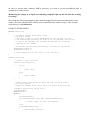
string variables' names begin with two '*' characters (although there are none defined at this version
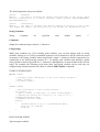
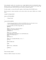
stage). For example, the following script shows how local string variables can be used, they are
assigned using comma separated lists (same as with the PRINT/print command).
START CUSTOM SCRIPT
HEADER counter
{
// A simple script showing how to use local string variables...
// And a counter...
// By Mauro Grassi...
}
SCRIPT counter
{
// The following is a local string variable...
*U=" events...";
// Open a counter on input #D0, it counts falling edges...
// Opening the counter also clears it, ie. sets it to 0...
@@openFallingCounter(#D0);
// Remember the last count...
while(1)
{
*A=”The Counter is up to “, @@readCounter(#D0);
print *A, *U, newline;
sleep(1);
}
}
END CUSTOM SCRIPT
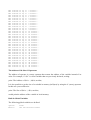
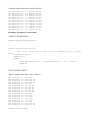
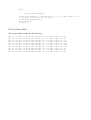
Typical output would be:
The
The
The
The
The
The
The
The
The
The
The
The
The
The
The
The
The
The
The
The
The
The
The
The
The
The
The
The
The
The
The
The
The
The
The
The
Counter
Counter
Counter
Counter
Counter
Counter
Counter
Counter
Counter
Counter
Counter
Counter
Counter
Counter
Counter
Counter
Counter
Counter
Counter
Counter
Counter
Counter
Counter
Counter
Counter
Counter
Counter
Counter
Counter
Counter
Counter
Counter
Counter
Counter
Counter
Counter
is
is
is
is
is
is
is
is
is
is
is
is
is
is
is
is
is
is
is
is
is
is
is
is
is
is
is
is
is
is
is
is
is
is
is
is
up
up
up
up
up
up
up
up
up
up
up
up
up
up
up
up
up
up
up
up
up
up
up
up
up
up
up
up
up
up
up
up
up
up
up
up
to
to
to
to
to
to
to
to
to
to
to
to
to
to
to
to
to
to
to
to
to
to
to
to
to
to
to
to
to
to
to
to
to
to
to
to
0 events...
0 events...
0 events...
0 events...
1 events...
2 events...
3 events...
4 events...
5 events...
6 events...
7 events...
8 events...
9 events...
10 events...
11 events...
12 events...
13 events...
14 events...
15 events...
16 events...
17 events...
18 events...
19 events...
20 events...
21 events...
22 events...
23 events...
24 events...
24 events...
24 events...
24 events...
24 events...
24 events...
24 events...
24 events...
24 events...
The Address Of & Size Of Operators
The address of operator is a unary operator that returns the address of the variable instead of its
value. For example, if “$A” is a local variable that was previously declared, writing:
print “The Address of $A is: “, &$A, newline;
It is also possible to get the size of a variable in memory (in Bytes) by using the '#' (unary) operator.
In this case you would write:
print “The Size of $A is: “, #$A, newline;
would print the address of the variable in local memory.
Built In Global Variables
The following global variables are defined:
Syntax:
Effect:
$$I2C
the I2C internal buffer
Syntax:
Effect:
$$SPI
the SPI buffer
Syntax:
Effect:
$$cache.file
base pointer to the FILE cache of the current script
Syntax:
Effect:
$$cache.ram
base pointer to the RAM cache of the current script
Syntax:
Effect:
$$cache.rom
base pointer to the ROM cache of the current script
Syntax:
Effect:
$$cache.stack
base pointer to the STACK cache of the current script
Syntax:
$$course
Effect:
32 bit floating point value indicating course over ground (heading)
in degrees set by the system if a GPS module is present and outputting valid GPS
GPRMC NMEA sentences through the serial port
Syntax:
Effect:
$$file
the memory mapped log file output for the VM
Syntax:
Effect:
$$fileName
the current script's log file name buffer
Syntax:
Effect:
$$hardware
base pointer to the hardware descriptors of the current script
Syntax:
$$hardware.I2C
Effect:
base pointer to the hardware descriptor for the I2C port of the
current script
Syntax:
Effect:
$$hardware.I2C.busRate
the current bus rate (in kHz) of the I2C port of the current script
Syntax:
$$hardware.SPI
Effect:
base pointer to the hardware descriptor for the SPI port of the
current script
Syntax:
Effect:
script
$$hardware.SPI.ckdidocspin
the CLK, DI, DO and CS pin register of the SPI port of the current
Syntax:
Effect:
$$hardware.SPI.mode
the current mode of the SPI port of the current script
Syntax:
$$hardware.oneWire
Effect:
base pointer to the hardware descriptor for the oneWire port of the
current script
Syntax:
Effect:
$$hardware.oneWire.mode
the current mode of the oneWire port of the current script
Syntax:
$$hardware.oneWireSerial
Effect:
base pointer to the hardware descriptor for the serial port of
oneWire port of the current script
Syntax:
$$hardware.oneWireSerial.baudRate
Effect:
the baud rate (divided by 10) of the serial port of the oneWire port
of current script
Syntax:
Effect:
$$hardware.oneWireSerial.mode
the current mode of the serial port of the oneWire port of the
current script
Syntax:
$$hardware.oneWireSerial.txrxpin
Effect:
the Tx and Rx pin register of the serial port of the oneWire port of
current script
Syntax:
$$hardware.serial
Effect:
base pointer to the hardware descriptor for the serial port of the
current script
Syntax:
Effect:
script
$$hardware.serial.baudRate
the baud rate (divided by 10) of the serial port of the current
Syntax:
Effect:
$$hardware.serial.mode
the current mode of the serial port of the current script
Syntax:
Effect:
$$hardware.serial.txrxpin
the Tx and Rx pin register of the serial port of the current script
Syntax:
Effect:
$$indirect
indirect memory access to [W]
Syntax:
$$latitude
Effect:
32 bit floating point value indicating latitude in degrees (<0
indicates South, >=0 indicates North) set by the system if a GPS module is
present and outputting valid GPS GPRMC NMEA sentences through the serial port
Syntax:
$$longitude
Effect:
32 bit floating point value indicating longitude in degrees (<0
indicates West, >=0 indicates East) set by the system if a GPS module is present
and outputting valid GPS GPRMC NMEA sentences through the serial port
Syntax:
Effect:
$$nmea.match.string
user defined NMEA match string command buffer
Syntax:
Effect:
$$nmea.match.stringPtr
NMEA match string command buffer pointer
Syntax:
Effect:
$$nmea.output
byte array contains the raw output of any NMEA sentence match
Syntax:
$$nmea.outputPtr
Effect:
position pointer to the byte array containing the raw output of any
NMEA sentence match (can be used to size the output)
Syntax:
Effect:
$$oneWire
the OneWire internal buffer
Syntax:
Effect:
$$oneWireRomCode
the OneWire Rom Code buffer
Syntax:
Effect:
$$por
is 1 if a POR (Power On Reset) has occurred, otherwise 0
Syntax:
$$return
Effect:
32 bit floating point return
returning values from local functions
value
variable,
can
be
used
for
Syntax:
Effect:
$$serial
the serial input pipe buffer
Syntax:
Effect:
$$serial.RxCRC
byte value used to accumulate the CRC checksum for the serial port
input pipe buffer (also used for NMEA sentence decoding)
Syntax:
Effect:
output
$$serial.TxCRC
byte value used to accumulate the CRC checksum for NMEA sentence
Syntax:
Effect:
$$serial.error
the last error status of the serial input pipe buffer
Syntax:
Effect:
$$serial.getPtr
the serial input pipe buffer read location pointer
Syntax:
Effect:
$$serial.lastRx
the last received character on the serial port
Syntax:
$$serial.newRx
Effect:
indicates that a new character has been received in the serial port
input pipe, cleared automatically when accessed using the global function
@@newRxUART
Syntax:
Effect:
$$serial.pipeState
the status of the serial input pipe buffer
Syntax:
Effect:
$$serial.putPtr
the serial input pipe buffer write location pointer
Syntax:
$$speed
Effect:
32 bit floating point value indicating ground speed in knots set by
the system if a GPS module is present and outputting valid GPS GPRMC NMEA
sentences through the serial port
Syntax:
Effect:
$$temp
temporary buffer (system limited)
Syntax:
Effect:
$$ven
base address of VM environment
Syntax:
Effect:
$$ven.vmExecLimit
VM environment execution limit
Syntax:
Effect:
$$ven.vmID
VM environment script ID buffer
Syntax:
Effect:
$$ven.vmLogFileCache
VM environment log file cache base address
Syntax:
Effect:
$$ven.vmLogFileName
VM environment log file name buffer
Syntax:
Effect:
$$ven.vmMinimumPeriod
VM environment minimum sleep period
Syntax:
Effect:
$$ven.vmMinimumSleepPeriod
VM environment minimum sleep period in seconds
Syntax:
Effect:
$$ven.vmMode
VM environment mode
Syntax:
Effect:
$$ven.vmNum
VM environment number of scripts loaded
Syntax:
Effect:
$$ven.vmPtr
VM environment script pointer
Syntax:
Effect:
$$ven.vmRecoveryTime
VM environment sleep recovery time in seconds
Syntax:
Effect:
$$ven.vmSelected
VM environment selected script
Syntax:
Effect:
$$ven.vmSleepPeriod
VM environment script sleep period
Syntax:
Effect:
$$ven.vmState
VM environment state
Syntax:
Effect:
$$vm
base pointer to the script structure
Syntax:
Effect:
$$vm.CRC
CRC check of the current script
Syntax:
Effect:
$$vm.DS
the DS register of the current script
Syntax:
Effect:
$$vm.DSLIMIT
the DS limit register of the current script
Syntax:
Effect:
$$vm.IR
the instruction register of the current script
Syntax:
Effect:
$$vm.PC
the program counter register of the current script
Syntax:
Effect:
$$vm.SS
the SS register of the current script
Syntax:
Effect:
$$vm.W
the accumulator of the current script
Syntax:
Effect:
$$vm.addressModes
the adressModes of the DS and SS registers of the current script
Syntax:
Effect:
$$vm.execDone
the execution counter register of the current script
Syntax:
Effect:
$$vm.execID
execution ID of the current script
Syntax:
Effect:
$$vm.execLimit
the execution limit register of the current script
Syntax:
Effect:
$$vm.execMode
execution mode of the current script
Syntax:
Effect:
$$vm.execPriority
the execution priority register of the current script
Syntax:
Effect:
$$vm.execState
execution state of the current script
Syntax:
Effect:
$$vm.lastError
last run time error of the current script
Syntax:
Effect:
$$vm.lastIndirect
the last indirect status register of the current script
Syntax:
$$vm.pipeMode
Effect:
the enabled pipes of the current script
Syntax:
Effect:
$$vm.resetVector
the reset vector register of the current script
Syntax:
Effect:
$$vm.sleepMode
the current sleep mode of the current script
Syntax:
Effect:
$$vm.stackSizePtr
the stack size/pointer register of the current script
Syntax:
Effect:
$$vm.temp
N/A
Syntax:
Effect:
$$vm.tempPipe
N/A
Syntax:
Effect:
$$vm.time
base pointer to the script's time register
Syntax:
Effect:
$$vm.time.day
day register of the script's time register
Syntax:
Effect:
$$vm.time.hours
hours register of the script's time register
Syntax:
Effect:
$$vm.time.mins
minutes register of the script's time register
Syntax:
Effect:
$$vm.time.month
month register of the script's time register
Syntax:
Effect:
$$vm.time.secs
seconds register of the script's time register
Syntax:
$$vm.time.show
Effect:
show register of the script's time register (determines which fields
of the time are shown)
Syntax:
Effect:
$$vm.time.updated
time updated register of the script's time register
Syntax:
Effect:
$$vm.time.wday
week day register of the script's time register
Syntax:
Effect:
$$vm.time.year
year register of the script's time register
Syntax:
Effect:
$$vm.timeOffset
N/A
Syntax:
Effect:
$$vm.timeScaling
N/A
Syntax:
Effect:
$$vm.timeSpeed
N/A
Syntax:
Effect:
$$vm.typeMode
the implicit argument type register of the current script
Built In Global Functions
The following global functions are defined:
Syntax:
Effect:
@@abs($1)
returns the absolute value of $1
Syntax:
Effect:
@@acos($1)
returns the arc cosine of $1 if $1 is between -1 and +1, otherwise 0
Syntax:
@@addDays($1, $2)
Effect:
if only one argument is given, add $1>0 days to the local time,
otherwise if $2==#vmTime, add $1 days to the script's time
Syntax:
@@addHours($1, $2)
Effect:
if only one argument is given, add $1>0 hours to the local time,
otherwise if $2==#vmTime, add $1 hours to the script's time
Syntax:
@@addMinutes($1, $2)
Effect:
if only one argument is given, add $1>0 minutes to the local time,
otherwise if $2==#vmTime, add $1 minutes to the script's time
Syntax:
@@addMonths($1, $2)
Effect:
if only one argument is given, add $1>0 months to the local time,
otherwise if $2==#vmTime, add $1 months to the script's time
Syntax:
@@addSeconds($1, $2)
Effect:
if only one argument is given, add $1>0 seconds to the local time,
otherwise if $2==#vmTime, add $1 seconds to the script's time
Syntax:
Effect:
@@asin($1)
returns the arc sine of $1 if $1 is between -1 and +1, otherwise 0
Syntax:
Effect:
@@atan($1)
returns the arc tangent of $1
Syntax:
Effect:
@@bcdToDecimal($1)
returns the decimal equivalent of the BCD value $1
Syntax:
Effect:
@@calibrateADC()
perform an automatic, real time calibration of the ADC system
Syntax:
Effect:
@@clearUART()
clears the serial port input pipe
Syntax:
Effect:
@@closeADC($1)
close pin $1 as analog input
Syntax:
Effect:
@@closeCapture($1)
close the frequency or counter input on pin $1
Syntax:
Effect:
@@closeI2C()
closes the I2C bus
Syntax:
Effect:
@@closeIO($1)
close the digital IO pin $1
Syntax:
Effect:
@@closeOneWire()
close the OneWire bus
Syntax:
Effect:
@@closeSPI()
closes the SPI bus
Syntax:
Effect:
@@closeUART()
closes the serial port
Syntax:
@@copyOneWireBufferToRomCodeBuffer($1)
Effect:
offset $1
fill the rom code buffer with the contents of the one wire buffer at
Syntax:
Effect:
offset $1
@@copyRomCodeBufferToOneWireBuffer($1)
copy the contents of the rom code buffer to the one wire buffer at
Syntax:
Effect:
@@cos($1)
returns the cosine of the angle (in radians)
Syntax:
Effect:
@@decimalToBcd($1)
returns the BCD equivalent of decimal value $1
Syntax:
Effect:
constant
@@exp($1)
returns the value of e to the power of $1, where e is the natural
Syntax:
Effect:
@@flashLED($1)
flash the onboard LED (LED3) on $1 times (system limited)
Syntax:
Effect:
limited)
@@flashLEDDuration($1, $2)
flash the onboard LED (LED3) on $1 times for $2 ms each time (system
Syntax:
Effect:
@@frac($1)
returns the fractional part of $1
Syntax:
Effect:
@@gcd($1, $2)
returns the greatest common divisor of $1 and $2
Syntax:
@@getADCRef()
Effect:
compute the ADC reference voltage by measuring (in real time) the
internal band gap reference voltage
Syntax:
@@getADCRefIfVBGVEquals($1)
Effect:
return the ADC reference voltage if the voltage of the band gap
reference (VBG) is $1
Syntax:
Effect:
@@getADCSupplyRef()
get the ADC reference voltage
Syntax:
@@getDay($1)
Effect:
if $1 is not given, get the day of the local time from the RTCC
(Real Time Clock Calendar), otherwise if $1==#vmTime, get the day of
script's time
the
Syntax:
@@getDaysInMonthYear($1, $2)
Effect:
if no arguments are given, returns the number of days in the local
time's month, otherwise returns the number of days in year $2 and month $1
Syntax:
@@getErrorUART()
Effect:
return the serial port input error register and then clear any
error. The error register can be a combination of the following constants:
#errorOverRunUART, #errorOverFlowUART, #errorUnderFlowUART
Syntax:
@@getHour($1)
Effect:
if $1 is not given, get the (24 hour time) hour of the local time
from the RTCC (Real Time Clock Calendar), otherwise if $1==#vmTime, get the
hours of the script's time
Syntax:
Effect:
@@getI2C($1, $2)
reads up to $2 bytes from I2C address $1 (into the $$I2C buffer)
Syntax:
@@getI2CTwoBytes($1)
Effect:
reads 2 bytes from I2C address $1 (into the $$I2C buffer)
Syntax:
Effect:
@@getIO($1)
get the level of the digital input pin on $1
Syntax:
Effect:
@@getLastRxUART()
returns the last received character from the serial port
Syntax:
@@getLocalTime()
Effect:
load the script's time register with the local time from the RTCC
(Real Time Clock Calendar)
Syntax:
@@getMinutes($1)
Effect:
if $1 is not given, get the minutes of the local time from the RTCC
(Real Time Clock Calendar), otherwise if $1==#vmTime, get the minutes of the
script's time
Syntax:
@@getMonth($1)
Effect:
if $1 is not given, get the month of the local time from the RTCC
(Real Time Clock Calendar), otherwise if $1==#vmTime, get the month of the
script's time
Syntax:
@@getPipes()
Effect:
return the currently enabled pipes. The result can be a combination
of
the
following:
#serialPipe,
#filePipe,
#usbPipe,
#fileNamePipe,
#systemLogPipe, #serialInPipe
Syntax:
@@getSeconds($1)
Effect:
if $1 is not given, get the seconds of the local time from the
RTCC (Real Time Clock Calendar), otherwise if $1==#vmTime, get the seconds of
the script's time
Syntax:
Effect:
@@getSizeUART()
returns the current size of serial port input pipe
Syntax:
@@getTotalSeconds($1)
Effect:
if no argument is given, return the total number of seconds from the
default time (1 Jan 2011 00:00:00) until the local time, otherwise if
$1==#vmTime, from the default time to the script's time
Syntax:
@@getTotalSecondsDiv($1, $2)
Effect:
if one argument is given, return the total number of seconds from
the default time (1 Jan 2011 00:00:00) until the local time divided by $1>0,
otherwise if $2==#vmTime, from the default time to the script's time divided by
$1>0
Syntax:
@@getTotalSecondsMod($1, $2)
Effect:
if no argument is given, return the total number of seconds from the
default time (1 Jan 2011 00:00:00) until the local time modulo $1>0, otherwise
if $2==#vmTime, from the default time to the script's time modulo $1>0
Syntax:
@@getUART()
Effect:
reads a character from the serial port input pipe, if available,
otherwise 0
Syntax:
@@getWeekDay($1)
Effect:
if no argument is given, return the week day of the local time,
otherwise if $1==#vmTime, return the week day of the script's time
(0=Monday, ..., 6=Sunday)
Syntax:
@@getYear($1)
Effect:
if $1 is not given, get the year of the local time from the RTCC
(Real Time Clock Calendar), otherwise if $1==#vmTime, get the year of the
script's time
Syntax:
@@initRandom($1, $2)
Effect:
initialises the pseudo random generator modulo $1 and with seed $2,
returns $2 modulo $1
Syntax:
Effect:
@@int($1)
returns the integer part of $1
Syntax:
Effect:
@@isIOHigh($1)
returns 1 if the digital IO pin $1 is high, otherwise 0
Syntax:
Effect:
@@isIOLow($1)
returns 1 if the digital IO pin $1 is low, otherwise 0
Syntax:
@@isLeapYear($1)
Effect:
if no argument is given, return 1 if the local time's year is a leap
year, otherwise return 1 if $1 is a leap year, otherwise 0
Syntax:
Effect:
@@isPrime($1)
returns 1 if $1 is prime, 0 otherwise
Syntax:
Effect:
@@ln($1)
returns the natural log of $1, if $1 > 0, otherwise 0
Syntax:
Effect:
@@log10($1)
returns the log base 10 of $1, if $1 > 0, otherwise 0
Syntax:
@@matchNMEAString()
Effect:
returns 1 if a NMEA sentence has been received on the serial port
input pipe and it matches the one last set using the built in matchNMEA command
Syntax:
@@newRxUART()
Effect:
returns 1 if a new character has been received on the serial port
input pipe for the script, otherwise 0
Syntax:
Effect:
@@notEmptyUART()
returns 1 if the serial port input pipe is not empty, otherwise 0
Syntax:
Effect:
@@numDivisors($1)
returns the number of divisors of $1
Syntax:
Effect:
@@oneWireCRC($1)
return the OneWire CRC of the $$oneWire buffer of up to $1 bytes
Syntax:
Effect:
@@openADC($1)
configure pin $1 as analog input
Syntax:
Effect:
@@openCapture($1, $2)
open pin $1 as a frequency/counter input in mode $2
Syntax:
Effect:
@@openCaptureHighFrequency($1)
open pin $1 as a high frequency input
Syntax:
@@openFallingCounter($1)
Effect:
open pin $1 as a counter input incrementing on a falling edge
(also clears the counter)
Syntax:
@@openFrequency($1)
Effect:
open pin $1 as a
frequency modes)
Syntax:
Effect:
frequency
input
@@openI2C($1)
opens the I2C bus running at $1 kHz
(with
automatic
scaling
of
Syntax:
@@openIO($1, $2)
Effect:
open a digital IO pin on pin
$2==#inputIO==1) of output (if $2==#outputIO==0)
$1
Syntax:
Effect:
@@openLowFrequency($1)
open pin $1 as a low frequency input
Syntax:
Effect:
@@openMediumFrequency($1)
open pin $1 as a medium frequency input
and
set
to
input
(if
Syntax:
@@openOneWire($1, $2)
Effect:
open the OneWire bus in mode $1 on pin $2. The mode can be a
combination of: #oneWireUsingUART, #oneWireUsingIO,
#oneWireOverDrive,#oneWireWrite, #oneWireRead, #oneWireStrongPullUp
Syntax:
@@openRisingCounter($1)
Effect:
open pin $1 as a counter input incrementing on a rising edge (also
clears the counter)
Syntax:
Effect:
CS pin $5
@@openSPI($1, $2, $3, $4, $5)
opens the SPI bus in mode $1, with CLK pin $2, DI pin $3, DO pin $4,
Syntax:
@@openUART($1, $2, $3, $4)
Effect:
opens the serial port in mode $1, baud rate $2 with Tx pin $3 and Rx
pin $4. The mode can be a combination of the following constants: #defaultUART,
#noTxInvUART, #noRxInvUART, #openDrainUART, #interruptRxUART (not currently
implemented), #noTxUART, #noRxUART, #GPSDecodingUART, #noUART
Syntax:
@@pauseVM($1)
Effect:
pause (if ($1 & #pause)!=0) or unpause (if ($1 & #noPause)!=0) the
script with ID $1
Syntax:
Effect:
@@primeProduct($1)
returns the product of the prime divisors of $1
Syntax:
Effect:
@@putI2C($1, $2)
writes up to $2 bytes to I2C address $1 (from the $$I2C buffer)
Syntax:
Effect:
@@putI2CByte($1, $2)
writes byte $2 to I2C address $1
Syntax:
Effect:
@@putI2CTwoBytes($1, $2, $3)
writes bytes $2 and $3 to I2C address $1
Syntax:
Effect:
@@putUART($1)
writes a character to the serial port
Syntax:
@@readADC($1)
Effect:
return
the
voltage
level
in
Volts
microcontroller corresponding to analog input pin $1
at
the
input
to
the
Syntax:
Effect:
regulator
@@readADCP()
return the voltage level in Volts at the input to REG1 the boost
Syntax:
Effect:
@@readComparator()
get the output state of the internal comparator (connected to S2)
Syntax:
Effect:
@@readCounter($1)
return the value of the counter on the pin $1 counter input
Syntax:
Effect:
@@readEE($1)
return the value of the byte of general non volatile memory at
address $1 (EEPROM emulated on memory card)
Syntax:
@@readEEFloat($1)
Effect:
return the 32 bit floating point value of general non volatile
memory at address $1 (EEPROM emulated on memory card)
Syntax:
Effect:
@@readFrequency($1)
return the frequency of the signal on the pin $1 frequency input
Syntax:
@@readV($1)
Effect:
return the voltage level in Volts at the analog input pin $1
(assuming the default voltage dividers have been used)
Syntax:
@@receivedNMEAUART()
Effect:
returns 1 if a valid NMEA sentence has been received on the
serial port input pipe, otherwise 0
Syntax:
Effect:
@@resetOneWire()
send a reset pulse to the OneWire bus
Syntax:
Effect:
@@rnd($1)
returns a pseudo random number modulo $1
Syntax:
@@sendOneWireCommand($1, $2, $3, $4)
Effect:
send the command $1, with data packet of $2 bits, in mode $3 and
with optional $4 ms pullup to the OneWire bus
Syntax:
@@sendOneWireCommandRomCode($1, $2, $3, $4)
Effect:
send the command $1, with data packet of $2 bits, in mode $3 and
with optional $4 ms pullup to the OneWire bus (Uses the Rom Code Buffer As
Buffer)
Syntax:
@@setADCSupplyRef($1)
Effect:
set the ADC reference
reasonable bounds
voltage
to
$1,
provided
it
is
within
Syntax:
@@setDay($1, $2)
Effect:
if only one argument is given, set the day of the local time to $1,
otherwise if $2==#vmTime, set the day of the script's time to $1
Syntax:
@@setHour($1, $2)
Effect:
if only one argument is given, set the (24 hour time) hour of the
local time to $1, otherwise if $2==#vmTime, set the year of the script's time to
$1
Syntax:
@@setIO($1, $2)
Effect:
set the digital output pin on pin $1 to high (if $2==#highIO==1) or
low (if $2==#lowIO==0)
Syntax:
Effect:
@@setLED($1)
set the onboard LED (LED3) on for $1 ms (system limited)
Syntax:
@@setLocalTime($1)
Effect:
set the RTCC (Real Time Clock Calendar) clock with the script's time
register or the argument $1 in the form time(YYYY:MM:DD:hh:mm:ss)
Syntax:
@@setMinutes($1, $2)
Effect:
if only one argument is given, set the minutes of the local time to
$1, otherwise if $2==#vmTime, set the year of the script's time to $1
Syntax:
@@setMonth($1, $2)
Effect:
if only one argument is given, set the month of the local time to
$1, otherwise if $2==#vmTime, set the month of the script's time to $1
Syntax:
Effect:
@@setSPICS($1)
set the SPI bus' CS line to $1
Syntax:
@@setScriptTime($1)
Effect:
set the script's time register, the argument $1 can be a time in the
form time(YYYY:MM:DD:hh:mm:ss)
Syntax:
@@setSeconds($1, $2)
Effect:
if only one argument is given, set the seconds of the local time to
$1, otherwise if $2==#vmTime, set the year of the script's time to $1
Syntax:
@@setShowScriptTime($1)
Effect:
set the show mode for the script's time register, where $1 is a
combination of the following constants: #showDay, #showWeekDay,
#showMinutes, #showSeconds, #showHours, #showMonth, #showYear, #showDefault
Syntax:
@@setTotalSeconds($1, $2)
Effect:
if only one argument is given, set the local time to the number
of seconds $1 from the default time (1 Jan 2011 00:00:00), otherwise
if $2==#vmTime, set the script's time at $1 seconds from the default time
Syntax:
@@setTotalSecondsDivMod($1, $2, $3, $4)
Effect:
if only three arguments are given, set the local time to the
number of seconds equal to (($1*$2)+$3) from the default time (1 Jan 2011
00:00:00), otherwise if $4==#vmTime, set the script's time at (($1*$2)+$3)
seconds from the default time
Syntax:
@@setVBGPinIO($1)
Effect:
if $1==1 enable the band gap reference voltage on the D5/A1 output
pin, if $1==0 disable such output
Syntax:
@@setYear($1, $2)
Effect:
if only one argument is given, set the year of the local time to $1,
otherwise if $2==#vmTime, set the year of the script's time to $1
Syntax:
Effect:
@@sin($1)
returns the sine of the angle (in radians)
Syntax:
@@sizeEE()
Effect:
get the size in bytes of the general non volatile memory (EEPROM
emulated on memory card)
Syntax:
Effect:
@@sqrt($1)
returns the square root of $1
Syntax:
Effect:
@@startVM($1)
add the script with ID $1 to the VM environment (start the script)
Syntax:
Effect:
script)
@@stopVM($1)
remove the script with ID $1 from the VM environment (stop the
Syntax:
@@sum($1, $2)
Effect:
returns the sum of $2 numbers starting at address $1, if $2 is
between 0 and 65535, otherwise 0
Syntax:
@@sumSquares($1, $2)
Effect:
returns the sum of the squares of $2 numbers starting at address $1,
if $2 is between 0 and 65535, otherwise 0
Syntax:
Effect:
@@sysRead($1)
return the value of the byte of system memory at address $1
Syntax:
@@sysReadFloat($1)
Effect:
$1
return the 32 bit floating point value of system memory at address
Syntax:
Effect:
@@sysWrite($1, $2)
write the byte $2 to system memory address $1
Syntax:
Effect:
@@sysWriteFloat($1, $2)
write the 32 bit floating point value $2 to system memory address $1
Syntax:
Effect:
@@tan($1)
returns the tangent of the angle (in radians)
Syntax:
Effect:
@@toggleIO($1)
toggle the level of the IO pin $1
Syntax:
@@writeEE($1, $2)
Effect:
write the byte $2 to general non volatile memory at address $1
(EEPROM emulated on memory card)
Syntax:
@@writeEEFloat($1, $2)
Effect:
write the 32 bit floating point value $2 to general non volatile
memory at address $1 (EEPROM emulated on memory card)
Syntax:
@@writeSPI($1)
Effect:
write $1 to the SPI bus, simultaneously return the value read from
the SPI bus
Syntax:
@@writeSPINoCS($1)
Effect:
write $1 to the SPI bus without asserting CS, simultaneously return
the value read from the SPI bus
Quick Templates: Example Scripts Follow
We now give a number of example scripts that show how to use the global functions to perform
some common logging tasks. These can be used as templates and customised as needed. All the
source code for these scripts is provided with the software/firmware code as well, to make them
easy to adapt to new logging tasks.
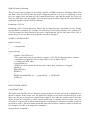
Reading an Analog Input
START CUSTOM SCRIPT
HEADER myAnalogSensorHeader
{
}
SCRIPT myAnalogSensorScript
{
// Basic Script Showing How To Read and Log an Analog Sensor
// By Mauro Grassi.
@@openADC(0);
PRECISION(1);
WHILE(1)
{
$T=(@@readV(0)-0.25)/0.028;
PRINT "The Temperature is: ", $T, " degrees Celsius.",newline;
SLEEP(5);
}
}
END CUSTOM SCRIPT
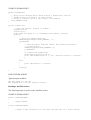
A typical output of the above script would be:
The
The
The
The
The
The
The
The
The
The
The
The
The
Temperature
Temperature
Temperature
Temperature
Temperature
Temperature
Temperature
Temperature
Temperature
Temperature
Temperature
Temperature
Temperature
is:
is:
is:
is:
is:
is:
is:
is:
is:
is:
is:
is:
is:
-8.9 degrees Celsius.
-8.9 degrees Celsius.
-8.9 degrees Celsius.
-8.9 degrees Celsius.
-8.9 degrees Celsius.
-8.9 degrees Celsius.
-8.5 degrees Celsius.
103.1 degrees Celsius.
103.5 degrees Celsius.
103.7 degrees Celsius.
103.2 degrees Celsius.
-8.6 degrees Celsius.
64.7 degrees Celsius.
Reading a Frequency/Counter input
START CUSTOM SCRIPT
HEADER myFrequencySensorHeader
{
}
SCRIPT myFrequencySensorScript
{
// Basic Script Showing How To Read and Log a Frequency Input, by Mauro
Grassi.
@@openFrequency(0);
PRECISION(3);
WHILE(1)
{
PRINT "The Frequency is: ", @@readFrequency(0), " Hz.", newline;
SLEEP(5);
}
}
END CUSTOM SCRIPT
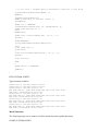
Typical Output of the above script would be:
The
The
The
The
The
The
The
The
The
The
The
The
The
The
The
The
The
The
Frequency
Frequency
Frequency
Frequency
Frequency
Frequency
Frequency
Frequency
Frequency
Frequency
Frequency
Frequency
Frequency
Frequency
Frequency
Frequency
Frequency
Frequency
is:
is:
is:
is:
is:
is:
is:
is:
is:
is:
is:
is:
is:
is:
is:
is:
is:
is:
0.000 Hz.
3012.048 Hz.
3012.048 Hz.
5319.149 Hz.
0.000 Hz.
180.044 Hz.
180.044 Hz.
180.044 Hz.
120.029 Hz.
120.029 Hz.
2.642 Hz.
2.642 Hz.
3.394 Hz.
7.519 Hz.
7.519 Hz.
7.519 Hz.
4504.505 Hz.
4504.505 Hz.
Reading an I2C sensor:
START CUSTOM SCRIPT
header myI2CHeader
{
// Basic Script Showing How To Read and Log a Temperature from an:
// AD7414 digital I2C sensor, by Mauro Grassi.
// Define a Constant which is the sensor's I2C Address
#I2C_ADDRESS=0x92;
}
script myI2CScript
{
// Open the I2C bus, running at 400kHz...
@@openI2C(400);
precision(3);
print "The Bus Speed is: ", $$hardware.I2C.busRate, newline;
while(1)
{
// Write the Address Register
$RESULT=@@putI2CByte(#I2C_ADDRESS, 0);
if($RESULT)
{
// Read Two Bytes From The Sensor (the address increments
// automatically)
$RESULT=@@getI2C(#I2C_ADDRESS, 2);
if($RESULT)
{
// Compute the Temperature
$T=$$I2C(0)+($$I2C(1)/256.0);
print "The Temperature is ", $T, " degrees Celsius.", newline;
}
}
else
{
print "Read Error.", newline;
}
sleep(3);
}
}
END CUSTOM SCRIPT
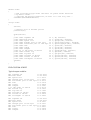
Typical output would be:
The Bus Speed is: 400.000
The Temperature is 25.875 degrees Celsius.
Reading a OneWire Sensor
The following script is used to read a OneWire sensor.
START CUSTOM SCRIPT
header oneWireReadROM
{
// Empty Header
}
script oneWireReadROM
{
// Sample Script showing how to discover the ROM code of a 1-wire sensor,
// in our case, a DS18B20 digital thermometer connected to pins D0-D1
@@openOneWire(#oneWireUsingUART, 0);
WHILE(1)
{
$RESULT=@@resetOneWire();
PRINT "Connecting to One Wire Sensor: ";
IF($RESULT)
{
PRINT "Ok.", NEWLINE;
@@sendOneWireCommand(0x33, 64, #oneWireRead, 0);
PRINT "The ROM Code is: ";
$A=0;
WHILE($A<8)
{
PRINT "0x", base($$oneWire($A), 16, 2), ".";
$A=$A+1;
}
PRINT NEWLINE;
@@copyOneWireBufferToRomCodeBuffer(0);
$A=0;
print "ROM Code: ";
while($A<8)
{
print base($$oneWireRomCode($A), 16, 2), ":";
$A=$A+1;
}
print newline;
}
ELSE
{
PRINT "Error.", NEWLINE;
}
SLEEP(3);
}
}
END CUSTOM SCRIPT
Typical output would be:
Connecting to One Wire Sensor: Error.
Connecting to One Wire Sensor: Error.
Connecting to One Wire Sensor: Ok.
The ROM Code is: 0x28.0xCB.0x8A.0xC2.0x02.0x00.0x00.0x7E.
ROM Code: 28:CB:8A:C2:02:00:00:7E:
Connecting to One Wire Sensor: Ok.
The ROM Code is: 0x28.0xCB.0x8A.0xC2.0x02.0x00.0x00.0x7E.
ROM Code: 28:CB:8A:C2:02:00:00:7E:
Connecting to One Wire Sensor: Ok.
The ROM Code is: 0x28.0xCB.0x8A.0xC2.0x02.0x00.0x00.0x7E.
ROM Code: 28:CB:8A:C2:02:00:00:7E:
Connecting to One Wire Sensor: Ok.
The ROM Code is: 0x28.0xCB.0x8A.0xC2.0x02.0x00.0x00.0x7E.
ROM Code: 28:CB:8A:C2:02:00:00:7E:
Maths Functions
The following script uses a number of built in maths functions (global functions).
START CUSTOM SCRIPT
header maths
{
// The following script shows the built in global maths functions
// By Mauro Grassi...
// Override the default behaviour, we want it to run only once...
execMode=#execModeNoRestart;
}
script maths
{
$A=-100;
// Display Up To 4 decimal places
precision(4);
while($A<100)
{
print "The argument $A
print "Absolute Value
print "The square root
print "The integer part of the sqrt
print "The fractional part of the sqrt
print "The sine
print "The cosine
print "The tangent
print "e to the power of $A/100
print "The natural log
print "The log base 10
print "The arcosine of $A/100
print "The arcsine of $A/100
print "The arctangent of $A/100
$A=$A+1;
}
}
END CUSTOM SCRIPT
Typical output would be:
The argument $A
Absolute Value
The square root
The integer part of the sqrt
The fractional part of the sqrt
The sine
The cosine
The tangent
e to the power of $A/100
The natural log
The log base 10
The arcosine of $A/100
The arcsine of $A/100
The arctangent of $A/100
is
is
is
is
is
is
is
is
is
is
is
is
is
is
63.0000
63.0000
7.9373
7.0000
0.9373
0.1674
0.9859
0.1697
1.8776
4.1431
1.7993
0.8892
0.6816
0.5622
The argument $A
Absolute Value
The square root
The integer part of the sqrt
The fractional part of the sqrt
The sine
The cosine
The tangent
is
is
is
is
is
is
is
is
64.0000
64.0000
8.0000
8.0000
0.0000
0.9200
0.3919
2.3479
is
is
is
is
is
is
is
is
is
is
is
is
is
is
",
",
",
",
",
",
",
",
",
",
",
",
",
",
$A, newline;
@@abs($A), newline;
@@sqrt($A), newline;
@@int(@@sqrt($A)), newline;
@@frac(@@sqrt($A)), newline;
@@sin($A), newline;
@@cos($A), newline;
@@tan($A), newline;
@@exp($A/100), newline;
@@ln($A), newline;
@@log10($A), newline;
@@acos($A/100), newline;
@@asin($A/100), newline;
@@atan($A/100), newline;
e to the power of $A/100
The natural log
The log base 10
The arcosine of $A/100
The arcsine of $A/100
The arctangent of $A/100
is
is
is
is
is
is
1.8965
4.1589
1.8062
0.8763
0.6945
0.5693
The argument $A
Absolute Value
The square root
The integer part of the sqrt
The fractional part of the sqrt
The sine
The cosine
The tangent
e to the power of $A/100
The natural log
The log base 10
The arcosine of $A/100
The arcsine of $A/100
The arctangent of $A/100
is
is
is
is
is
is
is
is
is
is
is
is
is
is
65.0000
65.0000
8.0623
8.0000
0.0623
0.8268
-0.5625
-1.4700
1.9155
4.1744
1.8129
0.8632
0.7076
0.5764
There are even more maths functions.
START CUSTOM SCRIPT
header imaths
{
// The following script shows the built in global maths functions
// By Mauro Grassi...
// Override the default behaviour, we want it to run only once...
execMode=#execModeNoRestart;
}
script imaths
{
$B[100]=0;
$A=1;
$counter=0;
print "The following numbers from 1 to 100 are primes: ", newline;
while($A<=100)
{
if(@@isPrime($A))
{
// store the prime number...
$B[$counter]=$A;
if(($counter % 8)==0)
{
print $A;
}
else
if(($counter % 8)==7)
{
print ", ", $A, newline;
}
else
{
print ", ", $A;
}
$counter=$counter+1;
}
}
}
$A=$A+1;
$A=0;
while($A<$counter)
{
print $A, ": ", $B[$A], newline;
$A=$A+1;
}
print newline, "There were exactly ", $counter, " primes found.", newline;
print "Their sum is: ", @@sum(&$B, $counter), newline;
END CUSTOM SCRIPT
Typical output would be:
The following numbers from 1 to 100 are primes:
2, 3, 5, 7, 11, 13, 17, 19
23, 29, 31, 37, 41, 43, 47, 53
59, 61, 67, 71, 73, 79, 83, 89
97
There were exactly 25 primes found.
Their sum is: 1060
Random Numbers
You can also use pseudo random numbers.
START CUSTOM SCRIPT
header random
{
// The following script shows the built in random number global
// functions... By Mauro Grassi...
// Override the default behaviour, we want it to run only once...
execMode=#execModeNoRestart;
}
script random
{
$B[100]=0;
$A=1;
$counter=0;
print "The following 100 numbers are randomly generated between 1 and 1000: ",
newline;
@@initRandom(1000, 41);
while($A<=100)
{
// store the prime number...
$R=@@rnd(1000);
$B[$counter]=$R;
if(($counter % 8)==0)
{
print $R;
}
else
if(($counter % 8)==7)
{
print ", ", $R, newline;
}
else
{
print ", ", $R;
}
$counter=$counter+1;
$A=$A+1;
}
print newline, "There were exactly ", $counter, " numbers generated.", newline;
print "Their sum is: ", @@sum(&$B, $counter), newline;
}
END CUSTOM SCRIPT
Typical output would be:
The following 100 numbers are randomly generated between 1 and 1000:
862, 103, 164, 445, 346, 267, 608, 769
150, 151, 172, 613, 874, 355, 456, 577
118, 479, 60, 261, 482, 123, 584, 265
566, 887, 628, 189, 970, 371, 792, 633
294, 175, 676, 197, 138, 899, 880, 481
102, 143, 4, 85, 786, 507, 648, 609
790, 591, 412, 653, 714, 995, 896, 817
158, 319, 700, 701, 722, 163, 424, 905
6, 127, 668, 29, 610, 811, 32, 673
134, 815, 116, 437, 178, 739, 520, 921
342, 183, 844, 725, 226, 747, 688, 449
430, 31, 652, 693, 554, 635, 336, 57
198, 159, 340, 141
There were exactly 100 numbers generated.
Their sum is: 46150
Logging the input to the serial port
A very common application is to log the input to the serial port. The following script accomplishes
just that, even toggling a LED to acknowledge the input. Note that when using the on board serial
port, the levels are 3.3V levels and may not be compatible with native serial ports that use different
voltage levels. You may need to add a small voltage translator circuit comprising a few transistors to
interface the hardware correctly.
START CUSTOM SCRIPT
header echoUARTToFile
{
// This script shows how to log the serial port input pipe onto the log
// file...
// It simply prints out any characters received on the serial port...
// By Mauro Grassi...
}
script echoUARTToFile
{
// open the serial port at 115200 bps, Tx on #D5 and Rx on #D4...
// open #D0 as a digital output, which we toggle to acknowledge reception
// of a character...
@@openIO(#D0, #outputIO);
// clear the log file for this script...
clearFile "echooutput.txt";
@@openUART(0, 115200, #D5, #D4);
@@clearUART();
while(1)
{
}
if(@@newRxUART())
{
// store the last received character...
$C=$$serial.lastRx;
// output the character to the log file for this script...
print char($C);
// continue!
// toggle the digital output!
@@toggleIO(#D0);
}
}
END CUSTOM SCRIPT
Using the serial Port As output
The following script shows how to use the serial port as an output pipe. It also shows how to
connect to a NMEA device (for eg, a GPS module) using the built in commands for NMEA
sentences. The USB Data Logger can automatically decode GPSS GPRMC NMEA sentences from
GPS modules such as the EM408 (available from Altronics). There is also software support for
matching arbitrary NMEA sentences and parsing the information contained in them.
START CUSTOM SCRIPT
header simpleGPS
{
// This script shows how to use the UART to connect to a GPS module such
// as the EM408 from Altronics, by Mauro Grassi.
// The USB Data Logger can automatically decode GPSS GPRMC NMEA sentences,
// but other NMEA sentences can be decoded as well...
}
script simpleGPS
{
// Create A new Log File for this script from scratch, "GPSDecoder.txt"
clearFile "GPSDecoder.txt";
// Initialise the UART, pin D0 is Tx, pin D1 is Rx...
// Baudrate 4800 bps is the default for the GPS module...
#D1);
// the special GPS decoding mode is enabled by using the define constant
// in the mode definition when opening the serial port #GPSDecodingUART...
@@openUART(#GPSDecodingUART + #noRxInvUART + #noTxInvUART, 4800, #D0,
print "Sending commands to the GPS module...", newline;
//
//
//
//
//
//
//
//
//
//
Refer to the datasheet of the EMS408 for details...
The nmea built in command sends the output to the serial port, but it
also keeps
a running XOR checksum that is appended to the end of the sentence for
error checking...
The NMEA CRC is sent by using the print function pf(#nmea), as shown
below. The following
command sets the output sentences for the EMS408 module to be GPSS //
GPRMC (recommended minimum
specific settings...
nmea "$PSRF100,1,4800,8,1,0", pf(#nmea);
nmea "$PSRF103,4,0,5,0", pf(#nmea);
print "Waiting for GPS Sentences...", newline;
precision(3);
while(1)
{
if(@@receivedNMEAUART())
{
print newline, "Rx: [", pf(#serialInPipe), "]", newline;
// #GPRMCNumBytesToMatch==32 is the number of bytes output
// by the internal automatic match for
// GPRMC sentences...
if($$nmea.outputPtr>=#GPRMCNumBytesToMatch)
{
print "Output: ", $$nmea.outputPtr, newline;
print newline, "Longitude: ", @@abs($$longitude), " ";
if($$longitude>=0)print "E"; else print "W";
print newline, "Latitude : ", @@abs($$latitude), " ";
if($$latitude>=0)print "N"; else print "S";
print newline, "Speed
: ", $$speed, " knots (over
ground)";
print newline, "Heading : ", $$course, " degrees ";
print newline, "GPS Time : ", pf(#vmTime), newline;
}
@@clearUART();
sleep(1);
}
}
}
END CUSTOM SCRIPT
Typical output from the above script is the following:
Rx: [GPRMC,113952.000,A,3244.0343,S,15005.6054,E,0.38,45.62,240111,,]
Output: 32.000
Longitude:
Latitude :
Speed
:
Heading :
GPS Time :
150.093 E
32.734 S
0.380 knots (over ground)
45.620 degrees
Mon 24 Jan 2011 11:39:52
Rx: [GPRMC,113955.000,A,3244.0360,S,15005.6020,E,0.90,240.94,240111,,]
Output: 32.000
Longitude:
Latitude :
Speed
:
Heading :
GPS Time :
150.093 E
32.734 S
0.900 knots (over ground)
240.940 degrees
Mon 24 Jan 2011 11:39:55
Rx: [GPRMC,113957.000,A,3244.0365,S,15005.6008,E,0.83,237.92,240111,,]
Output: 32.000
Longitude:
Latitude :
Speed
:
Heading :
GPS Time :
150.093 E
32.734 S
0.830 knots (over ground)
237.920 degrees
Mon 24 Jan 2011 11:39:57
In order to decode other, arbitrary NMEA sentences, you need to use the nmeaMatch built in
command, to set the pattern.
Monitoring the voltage at an input and switching a digital IO pin on and off when the reading
is in range
We include the following example to show how the digital IO pins can be switched under script
control. (Even the onboard LED (LED3) can be controlled from within a script!). This example
script also uses a local function.
START CUSTOM SCRIPT
HEADER monitoring
{
// A simple voltage monitoring script...
// By Mauro Grassi.
// Switches a digital IO pin HIGH whenever the voltage is above
// the maximum and switches the digital IO pin LOW when the voltage
// is below the minimum, the maximum and minimum are constants
// defined in the header...
// We define the switching thresholds, allowing for hysteresis...
#maximumVoltage=1.0;
#minimumVoltage=0.7;
// This example script also uses a local function...
}
SCRIPT monitoring
{
// Define a Local Function!
function @writeOnOff(1)
{
if($1)
{
print "ON";
}
else
{
print "OFF";
}
}
// Basic Script Showing How To Read and Log an Analog Sensor,
// by Mauro Grassi.
// Execution Begins here, after the local function definitions...
clearFile "monitoring output.txt";
@@openADC(#A0);
PRECISION(2);
WHILE(1)
{
$V=@@readV(#A0);
if(($V<#maximumVoltage) AND ($V>#minimumVoltage))
{
// within range, so don't do anything...
}
else
if($V<#minimumVoltage)
{
@@setIO(#D0, #lowIO);
}
else
{
@@setIO(#D0, #highIO);
}
print pf(#timeIfSet), " The Voltage is: ", $V, " The output is: ";
// we use a local function call here...
@writeOnOff(@@getIO(#D0));
print newline;
sleep(5);
}
}
END CUSTOM SCRIPT
This script produces output like the following:
Tue
Tue
Tue
Tue
Tue
Tue
Tue
Tue
Tue
Tue
25
25
25
25
25
25
25
25
25
25
Jan
Jan
Jan
Jan
Jan
Jan
Jan
Jan
Jan
Jan
2011
2011
2011
2011
2011
2011
2011
2011
2011
2011
00:22:44
00:22:49
00:22:54
00:22:59
00:23:04
00:23:09
00:23:14
00:23:19
00:23:24
00:23:29
The
The
The
The
The
The
The
The
The
The
Voltage
Voltage
Voltage
Voltage
Voltage
Voltage
Voltage
Voltage
Voltage
Voltage
is:
is:
is:
is:
is:
is:
is:
is:
is:
is:
1.20
1.19
1.02
0.49
0.00
0.39
0.65
1.11
1.36
1.36
The
The
The
The
The
The
The
The
The
The
output
output
output
output
output
output
output
output
output
output
is:
is:
is:
is:
is:
is:
is:
is:
is:
is:
ON
ON
ON
OFF
OFF
OFF
OFF
ON
ON
ON
We now describe the hardware and operation of the USB Data Logger, the following text is similar
to that which appeared in the original three articles in SILICON CHIP magazine (December 2010 &
January and February 2011)...
Universal USB Data Logger: Part 1
BY Mauro Grassi.
This simple project can log vast amounts of data onto a memory card. It consumes little power and
works using two AAA rechargeable (NiMH) or alkaline batteries, USB power or power derived
from another external source (between 5.5V and 7V DC). It can read many different types of digital
and analog sensors, and can even measure frequency. It has a real time clock and calendar for
making sense of the readings and connects to your PC using the USB. We also provide a PC host
program for Windows OSs that can be used to change the settings of the data logger and unlock all
its features.
Features at a glance:
•
•
•
•
•
•
•
•
•
•
•
•
•
Large storage using an MMC/SD/SDHC memory card (FAT file system);
USB Full Speed device (12Mbps) connection to PC and host PC program for Windows OSs;
Digital Sensor Support:
1. I2C (Inter-IC);
2. One Wire Dallas;
3. Full Duplex Serial Port UART (Universal Asynchronous Receiver Transmitter);
Analog Sensor Support: 12 bit ADC Voltage +/- 5% accuracy;
Analog Sensor Support: frequency signal up to 192kHz;
Analog Sensor Support: 32 bit counters;
Scripting Language allows many different sensors to be used;
Low Power (around 1.5mA in standby mode);
Flexible Power Options:
1. Battery Powered using two AAA batteries; or
2. USB powered; or
3. External 5.5V to 7V DC power source;
NiMH batteries can be recharged using USB power or external power source (trickle
charge);
Can connect an external voltage reference for greater than +/- 5% accuracy on ADC inputs;
Battery Protection to prevent over discharge;
Real Time Clock Calendar;
Introduction
This project is intended as a low cost and low power data logger that can collect vast amounts of
information onto a memory card, together with time and date information.
You can connect many different types of analog and digital sensors, and it is even possible to
connect a GPS (Global Positioning System) module to log space coordinates too.
Suppose you have a weather station, with humidity, wind speed, rainfall, temperature and
barometric pressure sensors. You can log their values over many days onto a CSV (comma
separated values) file on the memory card. Then connect the data logger to your Windows PC to
download the file through the USB (or simply using a memory card reader) and open it using Open
Office or MS Exel. It is then easy to graph the readings and analyse them.
In another application, you may want to diagnose a problem with your car's engine. You can
monitor the relevant sensors and log them while driving, then later analyse the data to find the
problem. You can even log your trajectory if you use a GPS module with the USB Data Logger.
There are many applications where this project would be useful, we've made it as flexible as
possible and able to accept many different types of sensors...
Circuit Description
The circuit for the USB Data Logger is shown in Fig.X. and is based around a PIC18F27J53
microcontroller from Microchip (IC1). We use the version in a slim (0.3") 28 pin through hole dual
in line package (SDIP).
The PIC18F27J53 is an 8 bit microcontroller with 128KB program memory and 3KB of SRAM and
is well suited to this application due to its impressive list of peripherals and low price.
The following are the peripherals that we use in this project: the USB device peripheral, the
integrated RTCC (Real Time Clock Calendar) with separate oscillator circuit, its low power "sleep"
modes (nanowatt XLP series), its serial peripherals (SPI, I2C, UART), DMA (Direct Memory
Access) support for the SPI peripheral, up to 10 output compare/capture peripherals, one of three
comparators, the 12bit ADC system with internal band gap reference, the comparator voltage
reference module, and the very useful PPS (Peripheral Pin Select) feature. Details of these are
discussed below.
Primary and Secondary Oscillators
The microcontroller uses two oscillators, the primary oscillator uses a 20MHz crystal (X1) and
associated 33pF ceramic loading capacitors, that provides the main system clock. The oscillator
output is divided by 5 and multiplied by 12 (using an internal PLL stage) to derive the single
48MHz clock used by the USB peripheral (USB Full speed device, 12Mbps) and the core. The core
runs at 12MIPs which is its highest rated speed. The firmware implements a full speed USB device
and connects to a PC using a USB cable via CON2, a USB Type B connector. We provide a driver
to use with Windows OSs, as well as instructions on how to install it, in a later article. The USB
Data Logger has its own VID (Vendor ID) and PID (Product ID) pair, sub licenced by Microchip.
Real Time Clock And Calendar
The secondary oscillator uses a 32.768kHz watch crystal (X2) and two 12pF ceramic loading
capacitors. This oscillator is almost always powered (even when the microcontroller is sleeping)
and is used for timekeeping by the RTCC peripheral inside IC1. This real time clock calendar
increments without firmware intervention to provide accurate timekeeping.
There are no switches to set the time and date, instead, the time is set using a Windows PC and the
USB connection. The time and date will be automatically synchronised with the PC once the host
program is used to connect to the USB Data Logger.
Battery Protection
The secondary oscillator is only switched off when the USB Data Logger goes into "deep sleep"
mode. This happens only if the firmware detects that the batteries are in a state of dangerously low
charge and in that case, the core is shut down and goes into deep sleep to prevent them from
discharging any further (which could damage them). In this special mode, the contents of the
SRAM are lost and the timekeeping will fail. This is done to minimise any further drain of the
batteries.
The USB Data Logger will require a reset – how to do this is explained in next month's article. This
should not happen in normal operation, however.
Note that when logging, the microcontroller spends most of its time sleeping (thus reducing the
power consumption) until the next logging timeout occurs. While sleeping, the RTCC still operates,
to maintain accurate timekeeping.
Flexible Power Options
The entire circuit of the USB Data Logger is powered from a 3.3V rail. This includes the
microcontroller and the memory card. While the microcontroller is powered by 3.3V, its core runs
from a 2.5V rail derived using an internal low drop out regulator. This regulator needs a decoupling
capacitor on the VDDCORE/VCAP pin (pin 6 of IC1), here we use a 10uF tantalum capacitor.
There is also a 100nF monolithic decoupling capacitor on the supply rail, close to the
microcontroller.
The 3.3V rail is derived using a low power synchronous boost regulator IC, the TPS61097-33 from
Texas Instruments (REG1). This switchmode IC can convert an input voltage between 0.9V and
3.3V into a regulated 3.3V rail that can supply up to 100mA to the circuit.
It uses a minimum of external components, just two capacitors and one inductor. In our case, we use
a 100uH RF choke for the inductor (L1) and a 22uF tantalum capacitor & a 220uF low ESR
electrolytic for bypassing. It comes in a space saving SOT-23 5 pin SMD (Surface Mount Device)
package that is, however, not difficult to solder by hand. We use tantalum capacitors for their small
size and high capacitance values.
This switchmode regulator is ideal in this application because of its superior efficiency over linear
regulators and allows the circuit to be powered from just two AAA cells. This has two main
advantages: cells are expensive, so using two rather than three decreases the cost, secondly, using
two AAA cells allows them to be trickle charged from a 3.3V rail since their voltage will not exceed
about 2.8V (when fully charged).
Power can be supplied in three ways: using two AAA batteries (there is a two pin header, CON5 to
connect the batteries), through the USB (5V supply via CON2) or through an external power source
of between 5.5V and 7V DC (the latter connects through pins 1 and 3 of CON3 – see Table.2 for a
complete pin out).
In the case that USB power or an external power source is used, a linear low drop out 3.3V
regulator (REG2) is used to first step down the voltage. A linear regulator is used here for its
simplicity and its poorer efficiency over the boost regulator is justified since we assume the power
source is either ultimately mains powered or powered by a substantial external battery.
REG2 is an LM3940 that can produce 3.3V from an input voltage as low as 5V. In our case, the
output of this regulator is fed, through a Schottky diode (D1), to the input of the switchmode
regulator (REG1). There is a tantalum 10uF capacitor on the input used for decoupling. We also use
a 47uF low ESR (Equivalent Series Resistance) aluminium electrolytic capacitor on its output, to
ensure stability. Do not be tempted to use a common electrolytic here, it must be low ESR. There is
also a 1k# resistor to ground to provide a minimal load.
The switchmode regulator steps up the voltage to the required 3.3V. The selection to use either USB
power or an external 5.5V to 7V DC source is made using the mini toggle switch (S1). Assuming
that only one of these is ever used, this toggle switch can function as a power switch, too.
The external power source has polarity protection using a single series Schottky diode (D4). As the
maximum input voltage to the LM3940 is 7.5V, and since the voltage drop of the Schottky diode
will be around 0.3V, we recommend that the input voltage at CON3 be strictly between 5.5V and
7V DC. We envisage that the most common use will be to connect a 6V SLA (Sealed Lead Acid)
battery or, if mains power is available, a 6V DC plugpack.
If you plan to use a 12V battery, you will not be able to connect it directly to this input. You could
use a simple LM7805 or LM7806 regulator between your 12V battery and the power input to the
circuit (at pin 3 of CON3) if you wish. Remember to provide bypass capacitors though. However, if
you want to use the data logger in your car, the easiest way is to purchase a USB charger that plugs
into your car's cigarette lighter socket and provides a regulated 5V.
In the absence of external power, the two AAA batteries provide power to the boost regulator
through a series Schottky diode (D2).
In our testing, we used two AAA 900-950mAh batteries (Jaycar: SB-1723, Altronics: S-4742C).
If AAA batteries and either the USB or external power source are used, the voltage produced by the
linear regulator (REG2) will trickle charge the batteries using a simple resistor to limit the rate of
charge.
This value of resistor is chosen so that the charging current is around 0.05*C (where C is the power
rating of the battery). This amount is considered safe for indefinite charging, and fully charging a
battery in this way can take up to 15 hours. Of course you can recharge the cells more quickly using
an external charger too, if you wish. In our case, we are presenting the project for use with two
900mAh NiMH batteries so we aim for a charging current of around 45mA (45=0.05*900).
Thus we choose a resistor of value approximately (3.0-2.5)/(0.045) = (approx) 10#. The regulator
can be assumed to output around 3.3-0.3=3.0V (since there is a series Schottky diode) and the
average voltage of two NiMH cells is around 2.5V (each cell will be between 1.1 and 1.4V in
normal operation, so we take an average).
Diode D2 bypasses the 10# resistor when no charging is taking place. Note that if you are using non
rechargeable, alkaline batteries, together with a power source, you should not install the 10# resistor
(R17). In this case, D2 provides reverse polarity protection against a reversed battery connection,
too.
Although the USB Data Logger is designed to be low power, and can run for long periods on just
two AAA batteries, for very long term logging, you should connect a 6V SLA battery.
Suitable batteries include the following: a 6V SLA battery, rated for say 12Ah (Jaycar: SB-2497) or
a number of 6V SLA 1300mAh batteries wired in parallel (Jaycar: SB-2495), which you can
recharge externally.
Memory Card
The USB Data Logger uses a memory card (MMC/SD/SDHC) for storage. They are ideal for this
application because they are of large capacity, cheap, easily acquired, low power and reliable.
Currently, capacities from 16MB up to 32GB are available.
A normally open (NO) switch inside the memory card socket (CON1) is used to detect when the
memory card is inserted into or removed from its socket. It has a single 33k# pull up resistor.
The memory card is powered by the 3.3V rail, but the supply to it can be controlled using Q1, a
2N7000 FET (Field Effect Transistor), which has its drain connected to the memory card's GND
connections.
The FET needs a substantial voltage at its gate to turn on properly, this is derived using a voltage
doubler circuit around diodes D3 and D5.
The basic doubler is formed using a 10nF green cap capacitor and D5 and is driven by the
microcontroller using a square wave generated by one of its output compare peripherals at the RP13
pin (pin 13 of IC1). When functioning as a doubler, the IO pin (pin 17 of IC1), that also controls
LED1, is brought high.
When the signal at RP13 is close to 0V, the 10nF capacitor charges to close to 3.3-0.6=2.7V through
D5 (0.6V is the voltage drop of D5, a 1N4004 diode). When the signal at RP13 goes high, the
capacitor is in series to effectively "double" the voltage at the cathode of D5 (well, close enough,
3.3+2.7=6V).
In other words, the signal at the cathode of D5 is a square wave of roughly double the amplitude of
the signal at RP13. This square wave is smoothed via diode D3 and the 4.7uF tantalum capacitor,
which form a "peak detector" circuit.
Now when functioning as a doubler, LED1 can be turned on for small periods (to flash) if
necessary, without affecting the gate voltage in any meaningful way.
This higher voltage is used to turn on Q1 through a 10# resistor. The latter is simply there to prevent
excessive currents to flow in the unlikely event that the thin insulating layer between gate and
channel inside Q1 is destroyed. The pull down 330k# resistor simply turns off Q1 in the absence of
a driving signal from the microcontroller. When power is cut to the memory card, the driving signal
from RP13 is stopped, and the IO pin simply controls the LED (except that it functions as an "open
collector" output, being either low (to turn on the LED) or tri-stated) (to turn the LED off)). The
firmware automatically adjusts the drive LED1 and the RP13 output as appropriate.
Using this circuit, the microcontroller can turn power to the memory card on or off. In periods of
extended idle time (ie, when not logging for extended periods), the microcontroller will go to sleep
and turn off the supply to the memory card, to conserve power. For short logging periods, the
memory card will not be turned off, as the initialization sequence would take too long relative to the
logging period. Therefore, the higher the frequency of logging the higher the power use – in actual
practice, this will be a compromise.
Memory Card SPI Connection
The SPI (Serial Peripheral Interface) peripheral of IC1 makes up the hardware interface to the
memory card. Higher level layers add support for a FAT (File Allocation Table) file system. This
file system has the advantage that it can be used with almost all operating systems in common use.
As to the hardware, MMC/SD/SDHC cards can be accessed in their native mode or in SPI mode.
The advantage of SPI mode is that it makes the hardware layer easy to implement. The interface
with SPI is simpler (but the penalty is slower transfer speeds). However, the SPI speeds are
adequate for data logging.
The microcontroller communicates with the memory card over one of the two on board SPI buses
(SPI2). It also has hardware support for DMA (Direct Memory Access) for the SPI peripheral,
which allows data to be transferred to and from the memory card transparently, while the
microcontroller is executing code. This makes the transfers very efficient.
SPI communication uses a four line bus and is capable of full duplex transfers between a host and a
slave. The four lines are: bar-CS (chip select - active low), SO (serial data output), SI (serial data
input) and SCK (serial clock).
In this case, the microcontroller is the SPI master and controls the bar-CS line. When it is pulled
low, the memory card becomes active and listens for commands.
The SPI peripheral is routed via the PPS (Peripheral Pin Select) feature of IC1, so that the SCK line
is at pin 21 and the SI and SO lines are at pins 18 and 22 respectively. The latter two are connected
(transposed) to the DO (Data Out) and DI (Data In) lines respectively of the memory card. These
lines are used to transmit and receive data in conjunction with the clock line (SCK) which is
generated by the microcontroller. The SPI bus runs at 12MHz in this application, which is the
fastest that the microcontroller will allow.
The bar-CS line is pulled high by a 33k# resistor to disable the memory card by default, and the
data output line from the memory card is also pulled high by a 33k# resistor.
Sensing the Supply Voltage
The microcontroller monitors the supply voltage to the boost regulator (REG1) using an ADC
(Analog Digital Converter) input (AN4 at pin 7 of IC1). The microcontroller can convert the analog
voltage at this pin to a 12 bit number.
When powered using two AAA batteries, this voltage will be at most around 2.7V (since the
maximum cell voltage is around 1.4V per cell and there is a Schottky diode in series with the
positive battery terminal).
On the other hand, when power is provided to REG2 (either through the USB or externally) the
voltage at this point will be close to 3V (since the output of REG2 is around 3.3V and there is also a
Schottky diode in series with its output).
Now the voltage at this point passes through a voltage divider formed from two 4.7k# resistors and
is bypassed using a 100nF monolithic capacitor. The microcontroller monitors the supply voltage
regularly. In the case that the batteries are dangerously low in voltage (indicating they have been
discharged too much), the microcontroller will take protective action, going into deep sleep, as
previously explained.
Pushbutton Action
Note that there is also a momentary SPDT switch (S2) that is in parallel with the lower 4.7k#
resistor of the divider. Pressing this switch brings the voltage at the AN4 pin close to GND and so
the microcontroller can detect that the pushbutton is being pressed and take appropriate action.
The firmware uses the output of an internal comparator to sense the switch press. The AN4 pin
shares its function with the C1INC pin, the latter is connected to the inverting input of an internal
comparator of IC1. The non-inverting input of the comparator is connected to an internal voltage
reference generated by a separate module inside the microcontroller.
This voltage reference can be controlled by the firmware and is derived using an internal resistor
ladder network from the supply voltage to IC1. The threshold is set at around 0.4V by the firmware,
meaning that any voltage at the AN4 input below this makes the output of the comparator go high.
Since there is a 2:1 voltage divider on this input, this means that the comparator goes low when S2
is not pressed and the voltage at the input to REG1 is above around 0.8V (which should always be
the case when the circuit is being powered). Hence the output of the comparator is normally low.
The comparator module is configured to generate an interrupt when the output of the comparator
goes from low to high (this happens when S2 is pressed). When this happens, a timer is started that
measures how long S2 is held down for.
The USB Data Logger recognises both a short press (less than a second) and a long press (more
than 1.5 seconds). Once the key press is registered, the timer is shut down (to save power) and the
firmware rearms the comparator interrupt after a hold off delay.
S2 can be used to start and stop the data logging, and for other functions, when the USB Data
Logger is connected to a PC. We will describe the user operation in more detail in next month's
article.
LED Indicator
The USB Data Logger has a single blue 3mm LED that is used to give feedback on the current
mode of operation, in the absence of a USB connection to a PC. The blue LED has a current
limiting 470# resistor and is driven using a single general purpose IO pin of the microcontroller
(RC6). In next month's article, we will cover what the LED indicates. Most of the time, the LED is
off to save power.
Extensive Sensor Support
This data logger can read many different types of sensors (that's why we are calling it a "Universal"
USB Data Logger). There are eight pins to connect external sensors, and they are accessed through
CON4, which is a terminal block. The pin outs are shown in Table.1, be sure to check the comments
for each pin. There are an additional four pins that make up CON3, also a terminal block. These are
power lines that can be used to supply external sensors or provide external power for the circuit
itself, the pinouts are shown in Table.2.
Pin
Pin
Number Name
Pin Function
Pin Comments
1
D0
Frequency
Input/Digital Digital Function, 0-3.3V signal output, 0-5V
Input or Output
signal input.
2
D1
Frequency
Input/Digital Digital Function, 0-3.3V signal output, 0-5V
Input or Output
signal input.
3
D2
Frequency
Input/Digital Digital Function, 0-3.3V signal output, 0-5V
Input or Output
signal input.
4
D3
Frequency
Input/Digital Digital Function, 0-3.3V signal output, 0-5V
Input or Output
signal input.
5
D4/A0
Analog/Frequency
Input Analog/Frequency Input 0-3.6V signal, can also
/Digital Input or Output
be used for digital functions.
6
D5/A1
Analog/Frequency
Input Analog/Frequency Input 0-3.6V signal, can also
/Digital Input or Output
be used for digital functions.
7
A2
Analog Input
Analog Input 0-13.8V signal.
8
A3
Analog Input
Table.1: shows the pinouts for CON4.
Analog Input 0-13.8V signal.
Pin Number
Pin Name
Pin Function & Comments
1
GND
Ground Reference (0V)
2
VDD
3.3V rail from REG1, can supply around 50mA max. for external
sensors. Always powered. Use this to supply small sensors that
consume little power.
3
VIN
Input for External Voltage Source (5.5V to 7V DC)
4
VDD (HIGH)
3.3V rail from REG2, can supply around 250mA max. as long as
either USB power or external power is present. Use this to supply
more power hungry "sensors".
Table.2: shows the pinouts of CON3.
Analog Sensors
The simplest sensors output a voltage proportional to the quantity they measure. For example, a
ratiometric temperature sensor would indicate the temperature by a varying output voltage that is
proportional to the ambient temperature.
Other sensors, such as accelerometers, can indicate acceleration on an axis by a varying voltage too.
Up to four analog sensors using voltage as the dependent variable can be used. There are two
different types of analog inputs, which form two pairs (A0 and A1 form one low voltage pair, while
A2 and A3 form a higher voltage pair). They only differ in the voltage divider ratio used.
For analog sensors with outputs between 0V and 13.8V, you should use analog inputs A2 and A3
(pins 7 and 8 of CON4). This is because each of these analog inputs have a voltage divider formed
by 15k# and 4.7k# resistors and are bypassed by a 100nF monolithic capacitor. Since the maximum
voltage that the microcontroller can digitize is around 3.3V, this gives the maximum voltage of
13.8V (13.8=3.3/(4700/19700)).
On the other hand, analog inputs A0 and A1 (pins 5 and 6 of CON4) use a volage divider formed by
470# and 4.7k# resistors (and are also bypassed by a 100nF monolithic capacitor). Therefore these
two inputs can accept voltages in the range 0-3.6V (4=3.3/(4700/5170)). The reason for the smaller
resistors on these two inputs is that it allows them to also be used for digital functions (then we refer
to them as D4 and D5 respectively).
Internal Voltage Reference
Note that the absolute accuracy of the 12 bit ADC conversion depends on knowing the exact supply
voltage to the microcontroller. While this is nominally 3.3V, in actual practice, it may be off by up
to +/- 0.1V due to manufacturing variations.
For this reason, the firmware will measure the supply voltage to IC1 regularly using an internal
band gap reference (1.2V +/- 5%) and adjust its readings accordingly.
Due to the error in the reference, the error in the digitised analog voltage value can be as high as +/5%, although it will be typically better.
This means that the error in the analog sensor readings will be at worst as high as this too.
Voltage Reference For Greater Accuracy
If higher than +/-5% precision is required for the analog sensors, a more precise voltage reference
can be connected to one of the four analog inputs. This reference can then be used to accurately
measure the other analog sensors. How to do this will be explained in next month's article.
The Universal USB Data Logger also accepts up to six frequency inputs, frequencies up to 192 kHz
can be measured. Up to two such inputs can be of amplitude up to 4V, while the others must be in
the range 0 - 5V. Note that the inputs D0 – D1 only have a pull up 4.7k# resistor to the 3.3V rail, but
the input pins in IC1 that they connect to are actually 5V tolerant. You can also use the frequency
inputs to act as simple counters, that increment on edge transitions (can count up to 32 bits).
Note that if you require greater voltage amplitude, you can of course change the voltage divider
associated with inputs D4/A0 and D5/A1, however, we won't cover how to do this here.
Digital Sensor Support
Not just varying voltage and varying frequency sensors can be connected, however. The great
flexibility of this design is that you can connect I2C, One Wire Dallas and serial port (UART)
sensors too. Problems to do with the inaccuracy of the ADC conversion are thus circumvented.
The I2C and One Wire connections are made using the digital input/outputs D0-D3 (pins 1-4 of
CON4).
There are 4.7k# pull ups to the supply rail on each of these lines, as required for both One Wire and
I2C operation (these buses use open collector outputs that need external pull ups, to allow multiple
devices to be connected to the same bus).
The great thing about using I2C sensors is that you can connect many different sensors to the same
I2C bus, which only requires two lines (as many as 127 I2C devices can be connected to the same
bus!). Similarly, only one line is required to connect many different One Wire Dallas sensors to this
data logger.
The Peripheral Pin Select feature of IC1 allows a number of on board peripherals to be routed to
different pins of the microcontroller. In this project, it is used to allow an output/input pin of CON4
to be reconfigured for different sensors.
There are six pins associated with digital sensors, labelled D0-D5 (pins 1-6 of CON4). Note that D4
and D5 share their function with analog pins A0 and A1. These two pins can function in only one
mode at any one time (ie, either digital or analog, but not both).
Finally, there is support for a configurable, full duplex serial port (UART) to be used. For example,
this allows a GPS module to be connected, such as the EM-408 featured in the October 2010 issue
of SILICON CHIP (Altronics: K-1131). This enables position, as well as time information to be
logged. You can also use the GPS module to gather accurate time information from the GPS
satellites rather than relying on the onboard RTCC. More on these options in next month's article.
Yes, you can even use the GPS module to synchronise the on board RTCC!
Scripting Language
The Universal USB Data Logger uses a scripting language to allow you to configure it to read many
different types of digital sensors. This is a powerful feature that allows the USB Data Logger to be
used with many different types of sensors, as each digital sensor is different in the interface that it
presents.
We've written a Windows PC host program that can parse a custom scripting language to interface
to many different types of sensors. The scripting language is compiled and the "machine code" is
programmed into the USB Data Logger's non volatile memory. Those images are then executed by
the microcontroller using a "virtual machine". This allows very complex arithmetic expressions to
be computed and logged, and makes this project a very powerful data logger.
We will explain how to use the scripting language in an upcoming article, as we've run out of room
this month. Stay tuned...
SC
Universal USB Data Logger: Part 2
BY Mauro Grassi.
In last month's first part we described the circuit of the Universal USB Data Logger and some of its
features. In this month's article, we give the full construction details, explain how to install the
Windows driver and software and outline how the data logger is used. As mentioned, the main
feature of this USB Data Logger is its Scripting Language, which makes it very versatile, this
allows it to interface to many different sensors easily.
Note: Although we have quoted the standby current consumption at around 1.5mA, this only
applies when the USB Data Logger is being powered from the two AAA cells. When using
either USB power or an external power source, the standby current is around 12mA due to the
higher consumption of the linear regulator. The assumption is that when using either USB or
external power, a bigger capacity power source is used, so the extra consumption is not an
issue.
Introduction
The USB Data Logger supports a custom scripting language which is its main feature and point of
difference from other data loggers. This allows it to interface to many different sensors easily. It
also makes it highly configurable and this means that if you have a logging application in mind, and
you are in doubt whether this data logger can be used for it, the answer is: almost certainly!
In this article, we guide you through the construction and installation of the Windows driver and PC
software. The latter is used to compile custom “scripts” that you can write to tell the data logger
how to read a sensor, and then tell it what to do with the data. This means that this data logger can
not only log data, it can also analyse the data! At the end of this article, we run through a number of
scenarios and give example custom scripts. These are a good starting point for learning to write
your own custom scripts. So let's run through a few things the USB Data Logger can do...
If you have a weather station, you can log a whole day's worth of temperatures and then compute
the average, or the daily maximum and minimum (say, in a spare time window at midnight).
If you have a number of digital sensors connected to the I2C bus, you can send commands to read
from them, log their values, or send commands to power them down during extended periods where
no logging needs to occur (the USB Data Logger itself will go to standby mode during extended
periods to save power).
You can read from a sensor and execute code depending on the reading reported by the sensor. For
example, if you have a temperature sensor, you can monitor its value and turn on or off an external
relay if the value is outside a specific range... These are just some examples of what is possible...
If you've ever programmed before, it should be very easy to understand and write programs for the
USB Data Logger (the scripting language's syntax is simple and loosely based on C).
We now explain how the USB Data Logger is built, it is a small and simple PC board and should
take only a few hours to assemble. If you purchase the USB Data Logger as a kit, it will be supplied
with a double sided PC board and all the specified components, including the preprogrammed
microcontroller.
Construction
The Universal USB Data Logger is built on a double sided PC board, coded 04112101 and
measuring 60 x 78 mm.
Before commencing, inspect the board for hairline cracks or unintended shorts between tracks. If
you are satisfied that the PC board looks ok, you can proceed. If you have any doubts about the
connectivity of tracks, you can use a DMM to check them.
Start the construction by soldering in the SMT (Surface Mount Technology) boost regulator (REG1)
which is a TPS61097-33DBVT in a SOT23 5 pin package. You will need a fine tipped soldering
iron and a steady hand.
This mounts on the top of the board. Position it over its pads (it can only go one way) and secure it
in position using some tape.
Make sure that you leave pin 5 uncovered, as this is the first pin to solder. Heat the pin and apply
the solder quickly, making sure never to apply heat for more than a few seconds. The solder should
melt easily and adhere to the pin and pad.
Let it cool. Once pin 5 has been soldered, you can proceed to solder in pin 3, which is diagonally
opposite. Once that is done, you can remove the sticky tape and proceed to solder the remaining 3
pins. If any solder bridges form, use solder wick to remove them (Altronics: T-1210, Jaycar: NS3026), also known as “de soldering braid”.
While you are on the top side of the PC board, you can solder in the memory card socket as well. It
has two small plastic feet that fit into holes on the PC board. This will anchor it in position over its
pads. Solder the two holding pads on its sides first, these will secure it in position. Once that is
done, you can proceed to solder in the rest of the pins – see photo. Again, use solder wick if you
accidentally create solder bridges between adjacent pins and be careful not to apply heat to the
plastic body, as it will melt.
Once that is done, you can proceed to install the resistors. The correct value must go in each place.
You should refer to the resistor colour code table in conjunction with the component overlay
diagram shown in Fig.X. It would be even better to check the resistors with a DMM to dispel any
doubt. Unlike most kits, due to space restrictions, the resistors are mounted vertically (see photo).
There are 5 Schottky diodes to go in next. Unlike the resistors, these need to be oriented correctly,
their cathodes are indicated by a grey stripe. The pad on the PC board that should connect to the
anode is shown on the top overlay silkscreen as an “A” - you can also refer to the component
overlay if in doubt.
The TO-220 regulator is next (REG2). It mounts horizontally on the PC board. You should bend the
leads by a right angle allowing around 7mm of lead. Secure it to the board with a single M3 nut and
screw before soldering (not after, as this can unduly stress the leads). Then proceed to solder in the
three leads.
The IC sockets can now be installed. If you don’t have a 28 pin 0.3” socket you can use two 14 pin
sockets. Be certain that the IC sockets are oriented to match the component overlay with their
notches in the right position. This will mean the microcontroller will be inserted with the correct
orientation later on.
Moving on, you will need to install the capacitors, making sure that the correct value and type is
placed in the corresponding place on the PC board. To do this, you should refer to the component
overlay. Note that there are four types: monolithic, ceramic, tantalum and electrolytic.
The electrolytic capacitor is polarised, and must be installed with the correct orientation. The
negative terminal is marked on the body of the capacitor and the positive terminal is marked on the
top overlay silk screen on the PC board using a “+” sign. Similarly, the tantalum capacitors have
their anodes indicated on their bodies by a “+” sign.
The two crystals should be installed next. The correct crystal must be installed in its designated
place, refer to the component overlay if in doubt. X1 is the 20MHz crystal while X2 is the smaller
32.768kHz crystal. For X2, its leads are delicate and you should take care with them. While X1
mounts so that it sits flush with the top of the PC board, X2 sits above the PC board, pushing it in
too far would over stress its thin leads. The same caveat applies to Q1, the 2N7000 FET. It can only
go in one way, and its leads should not be pushed too far as they can be overstressed too.
Next, install the two switches. One is a momentary pushbutton switch (S2) while the other is a mini
toggle switch (S1). Refer to the component overlay for their correct positions. They have three leads
that need to be soldered as well as a single mounting pin, which can be soldered to help anchor
them in place.
The 8 way and 4 way horizontal terminal block headers can go in next (clearly, they must face
outwards). It remains to install the 2 way pin plug for the battery, that also faces outwards.
While there, use the corresponding 2 way header socket (Altronics: P-5472, Jaycar: HM-3402) to
solder to the 2 AAA battery holder (Jaycar: PH-9226). Make sure you orient the positive (red wire)
and negative (black wire) correctly. The positive terminal on the PC board is to the right if facing
the connector and is indicated by a “+” on the top overlay silk screen (refer to the component
overlay if in doubt).
The USB TYPE B vertical mounting socket can go in next (see overlay). It has two mounting tabs
that secure it in place, and these can be soldered to their pads. Then solder the four small pads.
It remains to solder in the single 3mm blue LED. These should be soldered in with the correct
orientation, and you can cut out a 15mm cardboard spacer so that the LED's body sits at the correct
height from the PC board.
That completes the construction of the USB Data Logger, leave IC1, the microcontroller out of its
socket before continuing, we need to check the supply rail before we do that...
Powering Up for the First Time
You should use 2 AAA batteries to check the supply rails. We recommend you use 2 NiMH, 900950mAh batteries (Jaycar: PH-9226, Altronics: S-4742C). Of course, you can use any AAA NiMH
cells here, of more or less capacity, but you may have to change the 10# charging resistor in parallel
with D2, depending on your battery type. The formula to use was given in last month's Part 1
article.
If the 2 AAA batteries are not charged, you should charge them before proceeding. This may take a
few hours. A suitable charger is the Jaycar: MB-3549 or the Altronics: A-0283.
With the batteries charged, insert them into the battery holder and plug them into CON5 (also
marked with “BATT” on the top overlay silkscreen). Now measure, using a DMM, between pins 1
(GND) and 2 (VDD) of CON3. You may need to plug in the 4 way screw terminal socket before
you do this. In any case, you should measure close to 3.3V here. If you don't, disconnect the
batteries immediately and recheck your work. Check around REG1, you can measure the voltage at
its input and its output. If you are not measuring much voltage at the output at all, it could be
because diode D2 is incorrectly orientated.
If you did measure close to 3.3V, all is ok and you can disconnect power. Now insert IC1 into its 28
pin socket, making sure it is correctly orientated with its notch matching the component overlay.
Installing in the Specified Case
If you've checked the voltage rails are OK, you can proceed to install it in its specified case. The
USB Data Logger was designed to fit in a plastic instrument case (Altronics: H-0342 or H-0343). It
mounts using four of eight screws supplied with the case (7 mm long) – see photo.
The cut outs diagrams for the case are shown in Fig.X. There are 5 cut outs required on the 'bottom'
piece of the case – one each for the two switches, one each for the two terminal blocks, and one slot
for the memory card. Additionally, there are two cut-outs required on the 'top' piece of the case, one
for the USB socket, and one for the blue 3mm LED.
The 2 x AAA battery holder solders straight to the PC board and is stored in the battery
compartment of the case, for easy access. You can either glue it to the 'top' piece or screw it to the
'top' piece, but we've left it unattached for our prototype.
The two pieces of the case are held in place using an additional four screws, also supplied with the
case. Of these, two are 20mm long and are used for the two top holes (in the normal orientation
with the memory card at top) while the rest are 9mm long and are used for the two bottom holes.
These four screws mount through the bottom of the bottom piece upwards (the two bottom holes are
not normally visible on the bottom of the bottom piece of the case, but they can be accessed by
opening the battery compartment).
That completes the construction of the USB Data Logger, and you can proceed to installing the PC
software to use with it.
Installing the Windows Driver and Software
The USB Data Logger requires that a driver be installed on your Windows PC for it to work with
your PC and the supplied PC host program. The installation of the driver is easy and only needs to
be done once. In this section, we give a step by step guide on how to do this, as follows.
After the driver installation, we cover how to install the Windows software.
Assuming you have followed the construction instructions, you should now have a fully operational
USB Data Logger. You will need a Type A to Type B USB (Full Speed) cable.
A suitable (single) USB cable can be purchased from Jaycar or Altronics (Jaycar: WC-7700,
Altronics: P-1911A). In any case, these cables are common place these days and one should be easy
to acquire.
The supplied Libusb driver should work with all Windows versions including 64 bit Windows 7
versions with which we've developed this project.
We give the instructions for installing the driver on a Windows 7 machine, but the procedure is
similar for other Windows versions.
Unzip the contents of the file usbdatalogger.zip to a directory on your hard disk (this can be done
by right clicking on the file and choosing “Extract All...”). The file can be downloaded from the
downloads area of the SILICON CHIP website. This zipped archive contains both the driver and the
PC host software files.
Then connect the USB Data Logger (after you've checked that it is working correctly) to your PC
using the USB cable. You don't need batteries for this, since it can be powered directly from the
USB port by moving switch S1's position to up.
Windows should recognise the new device, and prompt for the installation of the driver. It may then
try to install the driver automatically, but this will fail because the driver won't be part of the driver
database yet.
You will get the message 'Device Driver Software was not successfully installed'. Go to 'Control
Panel>Device Manager'. A window should appear similar to the one shown in Fig.X.
You will see the device 'USB Memory Card Data Logger' with an exclamation mark. Select it and
right click. Select the 'Update Driver Software' option. A window similar to the one shown in Fig.X
will appear. Choose 'Browse my computer for driver software'.
An open file dialog will appear and you should navigate to the directory where you unzipped the
driver files using the 'Browse' button as shown in Fig.X.
Choose the 'USBMemoryCardDataLogger.inf' file that appears. On recent Windows OS versions
(eg, Vista and Windows 7) a security message will appear as shown in Fig.X.
Click 'Install this driver software anyway'. Windows should then proceed to install the driver. This
may take a few minutes depending on your system. Once complete, a window should appear saying
that 'Windows has successfully updated your driver software'.
If the driver is installed correctly, you should be able to see the USB Data Logger in Device
Manager (of course, it needs to be connected using a USB cable and powered on) under the 'LibusbWin32 Devices' group.
That completes the installation of the driver!
Launching the PC Host Software For Windows
To use the USB Data Logger with a Windows PC, you use the included executable program
usbdatalogger.exe. It is included in the zipped archive you downloaded and extracted earlier that
also contains the Windows driver files. You may want to create a shortcut to this file on your
desktop, for easy access. If so, right click on it and choose “Send To Desktop”.
Once that is done, you can launch the program by clicking on the desktop icon, easy. The PC host
program connects to the USB Data Logger and can be used to compile custom scripts, transfer files
to and from the USB Data Logger and a few other functions.
You can run the executable program to get the window shown in Fig.X.
Overview of the PC Host Program
The PC host program supplied can be used to compile, simulate and load custom scripts onto the
USB Data Logger. It also allows files to be transferred to and from it, to download logs and
configure the USB Data Logger (as well as synchronising the real time clock). Note that since all
files are stored in a FAT filesystem, the memory card can also be connected directly to a PC with a
memory card reader, or through a USB memory card reader. This would be desirable if transferring
very large files (more than 15MB say) as it can access the memory card substantially faster than the
USB Data Logger's microcontroller can.
The PC host program is based around a Windows GUI (Graphical User Interface) and was written
in Visual C++. The custom scripting language compiler and parser were also written in C++ (with
help from the open source parser and lexical analyser generators, Bison and Flex). The VM engine
was written using the full version of the C18 compiler, donated by Microchip.
When running, and the USB Data Logger is connected (with the driver installed) the PC host
program will detect it automatically. You will then be able to write, compile and send custom
programs to the USB Data Logger (each script is a separate file).
You can also transfer files, update the real time clock, and other functions. The main feature is the
custom scripting language support, and we describe this next.
Introduction to the Scripting Language
The scripting language is a light weight functional language implemented on a virtual machine that
incorporates virtual memory support and a (modified) Harvard architecture. The best way to start is
to see some sample code, which we present in the sections that follow. The PC host program
converts the source code to machine code that then executes on the USB Data Logger.
At this stage, it's customary to give the “Hello World” program, which looks like this:
START CUSTOM SCRIPT
HEADER helloWorldHeader
{
// Empty header
}
SCRIPT helloWorldScript
{
// Simple Hello World program for the USB Data Logger, by Mauro Grassi
PRINT “Hello World”, NEWLINE;
}
END CUSTOM SCRIPT
A script consists of a header declared by the HEADER keyword, followed by its name (which you
can choose) followed by the header's body enclosed in curly brackets. The header can contain
settings to alter the default behaviour of the script, but in most cases, its body will be empty and the
defaults can be used.
In these examples, we've used capital letters for all the keywords, to easily identify them, but the
compiler accepts keywords in lower case letters as well (ie, all lower case or all upper case letters, it
is a syntax error to have a combination of upper and lower case letters for keywords, eg HEADER
and header are both OK, but heAder is not).
Note that all other parts of the compiler are case sensitive. The compiler will give useful error and
warning messages, together with the line and column number of the error/warning. This makes it
easy to fix any syntax errors.
The header is followed by the script's body of code. This is similarly defined using the SCRIPT
keyword, followed by the name of the script, followed by the custom script code, again enclosed in
curly brackets. Lines starting with two slashes are comments and are ignored by the compiler (like
C). Curly brackets are used to group statements, which are always terminated by a semi colon.
In this case, the script has a single command, PRINT which takes the argument “Hello World” (a
string) and a newline. The arguments to the PRINT command are separated by commas. The output
is actually written to the log file for that script (each script has its own log file – although it is also
possible for a script to write another script's log file too).
That's the first program, we now run through a number of scenarios and each section presents a
custom script to do a particular task. We've chosen the most common types of tasks that people
would want to do... Sample code can also be downloaded from the SILICON CHIP website.
Reading An Analog Sensor
One of the most common things you'll want to do is to log a voltage varying over time. The USB
Data Logger has four analog inputs which can be used for this purpose, labelled A0-A3. Remember
that two of the analog sensors are for low voltages (0-3.6V) and two are for higher voltages (013.8V), as explained in last month's first part. They simply differ only in the voltage divider used.
Your analog sensor would typically have a voltage proportional to the measured quantity (ie, be
ratio metric). In this example, we'll cover how to connect an Analog Devices AD22103 temperature
sensor, there are many different types of analog sensor and you will have to consult the datasheet
for your device to configure it properly. But the general method should be similar to this example.
The AD22103KTZ is a three pin temperature sensor in a TO-92 package. Two pins are for the
supply (3.3V) and the third pin is the voltage output, proportional to temperature and between 0 and
3.3V. While many analog sensors are ratiometric, they may differ in the specific “linear transfer
function”. Luckily, all can be used with this data logger.
To connect it, connect the output pin to one of the four analog input pins, in this example, we'll use
A0 as it is suitable for 0-3.6V.
The transfer function of the AD22103 temperature sensor is, according to its datasheet, given by:
Vo = (Vs/3.3)(0.25 + 0.028T)
where Vo is the voltage at its output terminal, Vs is the supply voltage to the sensor and T is the
temperature (between 0 and 100, in degrees Celsius). For the sake of simplicity, let's assume that
Vs=3.3, so the equation becomes:
Vo=0.25 + 0.028T
Rearrange this equation to get the temperature as a function of the output voltage:
T= (Vo-0.25)/(0.028)
A custom script to read this sensor and log its value every minute would be the following:
START CUSTOM SCRIPT
HEADER myAnalogSensorHeader
{
}
SCRIPT myAnalogSensorScript
{
// Basic Script Showing How To Read and Log an Analog Sensor, by Mauro Grassi.
@@openADC(0);
PRECISION(1);
WHILE(1)
{
$T=(@@readV(0)-0.25)/0.028;
PRINT “The Temperature is: “, $T, “ degrees Celsius”, newline;
SLEEP(60);
}
}
END CUSTOM SCRIPT
This script is largely self explanatory, we run through a few basics that are not obvious. Variables
(which store data, as 32 bit floating point numbers) and Functions (which execute code) can be both
Local and Global. Local ones can only be accessed by the custom script and are defined there.
Globals can be accessed by all running scripts and are implemented internally.
Execution begins at the @@openADC(0); statement. As mentioned, each statement ends with a
semi-colon (like in C). The @@openADC statement is a built in global function.
Full details of the custom scripting language's syntax, built in functions, built in global
variables can be downloaded from the SILICON CHIP website, in the Jan 2011 downloads
folder.
Their names always start with two '@' characters (so it's easy to tell which are built in functions and
which are user defined functions, the latter always start with only one '@' character). Now this
particular function takes one argument, which is the channel number.
In this case @@openADC(0); simply configures the A0 pin as an analog input. The next statement,
PRECISION(1); is a built in command (rather than a built in global function).
It simply configures the number of decimal points for printing floating point values, used later on to
display the temperature. Then the program enters its “main loop” where it will execute its infinite
loop. This is the WHILE(1) built in command that executes the block of code enclosed in its curly
brackets whenever the condition is non zero (as in C). The next line reads:
$T=(@@readV(0)-0.25)/0.028;
and should be self explanatory. There are built in rules for which arithmetic operators take
precedence over others (for eg, multiplication takes precedence over addition, so that 8*3+2=26
rather than 40) but you can use brackets whenever in doubt. Apart from the four arithmetic
operators, you can also use the ^ (exponent) and % (modulo) operators (note that unlike in C, ^ is
used for XOR).
The statement simply computes the temperature $T by reading the voltage at channel 0 (using the
built in global function @@readV, subtracts 0.25 from the value and divides the result by 0.028). It
stores the result in the local variable $T. Local variables are “local” to the current script, so cannot
be accessed by other running scripts (as opposed to global variables which can). Local variables
always start with a single '$' character. Global variables always start with two '$' characters (in
analogy with global and local functions). Once the temperature is computed and stored in the local
variable $T (which is a 32 bit floating point value), the next statement logs the result into the
memory card.
A typical line would read:
The temperature is: 21.4 degrees Celsius
PRINT is a built in command and it takes as argument a comma separated list. Each item in the list
is either a constant string, enclosed in quotes (“), or an expression (in this case the value of $T), or a
special print command. In this case, we are using the NEWLINE print command, to add a line
return to the log file.
The last line is another built in command, SLEEP and it takes a single numeric argument, which is
the number of seconds to suspend execution of the script for. It simply puts the script to sleep for
the specified period, letting other scripts run. The script will be awoken after this period and begin
execution after the SLEEP command. In this case, since it is the last statement in the WHILE loop,
a new value will be read and logged and the process will repeat indefinitely...
There is another command for sending a script to sleep, it is the SLEEPUNTIL command (or
sleepUntil if in lowercase).
Unlike the SLEEP command, it takes an absolute time (in the future), as argument. For example,
writing:
SLEEPUNTIL(16:00:10);
will suspend the execution of the script until just after 4pm.
Now suppose you wanted to display the reading as Fahrenheit as well. Then you could change the
PRINT statement to:
PRINT “The temperature is: “, $T, “ degrees Celsius, or “, ($T*(9/5)+32), “ degrees Fahrenheit”,
NEWLINE;
Logging the Time
Another thing you can do is time stamp the logging. You can do this using one of the built in print
functions, PF(#TIME) (PF stands for PRINT FUNCTION and is used with the built in PRINT
command). In this case, you would replace the PRINT statement with the following:
PRINT PF(#TIME), “ The temperature is: “, $T, “ degrees Celsius”, NEWLINE;
Reading A Frequency Input
Reading a frequency rather than a voltage is just as easy. The basic script would look like the
following:
START CUSTOM SCRIPT
HEADER myFrequencySensorHeader
{
}
SCRIPT myFrequencySensorScript
{
// Basic Script Showing How To Read and Log a Frequency Input, by Mauro Grassi.
@@openFrequency(0);
PRECISION(3);
WHILE(1)
{
PRINT “The Frequency is: “, @@readFrequency(0), “ Hz”, newline;
SLEEP(5);
}
}
END CUSTOM SCRIPT
In this case, after initalizing the frequency input, and setting the PRINT PRECISION to 3 decimal
places, the main loop begins executing and logging the frequency on that pin in Hz, every 5
seconds. Note that the frequency can be anywhere between 0.1Hz and 192kHz. To cover this wide
range, three different modes are used (LOW, MEDIUM and HIGH frequency), and the mode will be
changed automatically by the firmware to suit the frequency (to achieve the best accuracy). For
example, for frequencies below about 1kHz, a special LOW FREQUENCY mode is used, whereas
above around 12kHz a special HIGH FREQUENCY mode is used instead.
Reading a Counter Input
Reading a 32 bit counter value is just as easy as logging a frequency input. In this case, simply
replace the @@openFrequency(0); statement by either a “@@openRisingCounter” or
“@@openFallingCounter” statement (selecting to increment the count on a rising or falling edge),
and replace the @@readFrequency(0); statement by a “@@readCounter(0)” statement (of course,
you should change the PRINT statement to suit your needs). Note that for counters, the value is
cleared (set to 0) whenever it is opened. So the counter can be “reopened” to clear it.
Reading an I2C Temperature Sensor
In this section, we cover how to read from a digital temperature sensor using the I2C bus. For this
example, we are going to use the Analog Devices AD7414 temperature sensor. It is a 10 bit
temperature to digital converter, using the I2C bus. The one we are using comes in a SOT-23 6 pin
package. Two pins are for the supply voltage, which is 3.3V so can be powered directly by the USB
Data Logger. There are two pins (AS and ALERT) which are input and outputs respectively. The AS
input can be used to choose one of three I2C addresses (to potentially use more than one of these on
the same bus) (the three addresses are chosen by a high, low or floating pin). We've configured ours
so that the I2C address is 0x92 (hexadecimal).
The ALERT output pin will change if configured, when the temperature exceeds the set limits. We
are not using this feature in this example, but you could write your own custom script to do just this.
The remaining two pins are the SCL (clock) and SDA (data) lines of the I2C interface, and these
should connect to the digital pins D0 and D1 respectively on the USB Data Logger.
Reading the datasheet of the AD7414 sensor tells you how to read the temperature value. This
particular sensor is used by reading and writing to 4 internal 8 bit registers. One register (at address
0) holds the MSB 8bits of the value (you can just read this for a good approximation, or read again
the extra 2 bits for the full resolution). Address 1 holds the “Configuration Register”, which holds
the extra 2 bits of temperature information, as well as extra bits to control the power to the sensor
(you can put it in standby to save power, and set the alert function mentioned above). The other two
registers hold the Minimum and Maximum Temperatures for the alert function, which we don't use
in this example.
The way writing works is as follows: the first write sets the address of the next write. For example,
if we want to write to the register at address 2, we first write 2 and then the value to write to at
address 2.
Similarly for reading, you first write the address, then read from the sensor. So to read the value at
address 1, for example, you first write 1 and then read from the device (one byte).
A program to read the temperature from the AD7414 is as follows:
START CUSTOM SCRIPT
HEADER myI2CHeader
{
// Basic Script Showing How To Read and Log a Temperature from an:
// AD7414 digital I2C sensor, by Mauro Grassi.
// Define a Constant which is the sensor's I2C Address
#I2C_ADDRESS=0x92;
}
SCRIPT myI2CScript
{
// Open the I2C bus, running at 400kHz...
@@openI2C(400);
PRECISION(3);
WHILE(1)
{
// Write the Address Register
$RESULT=@@putI2CByte(#I2C_ADDRESS, 0);
if($RESULT)
{
// Read Two Bytes From The Sensor (the address increments automatically)
$RESULT=@@getI2C(#I2C_ADDRESS, 2);
if($RESULT)
{
// Compute the Temperature
$T=$$I2C(0)+($$I2C(1)/256.0);
PRINT "The Temperature is ", $T, “ degrees Celsius”, NEWLINE;
}
}
else
{
PRINT "Error", NEWLINE;
}
SLEEP(30);
}
}
END CUSTOM SCRIPT
In this script, we first define a constant #I2C_ADDRESS in the header (it can also be defined in the
script). We then use it in all places of the code that take the I2C address of the sensor as an
argument. This is a good thing to do, since if we later want to change the I2C address, we simply
need to change one value (the 0x92) rather than all places where it is used... Define constants
always start with a '#' character, which is supposed to be reminiscent of the “#define” preprocessor
directive in C. Note that these define constants can be redefined but the compiler will warn you if
this happens.
We first open the I2C bus and declare it to run at 400kHz, using the built in global function
@@openI2C. We then set the precision to 3 decimal places and enter the main loop.
We declare a local variable called $RESULT which takes the value returned by the built in global
function @@putI2CByte. The latter takes two arguments. The first is the I2C address, the second is
the single byte to write to the I2C bus. In this case, we simply write 0 to the sensor, to set the
address (0-3 to read from). In this case, we are interested in reading addresses 0 and 1 so we write 0.
The @@putI2CByte function returns a value of 1 if the command succeeded or 0 otherwise. For
example, if there is no sensor connected, the function will fail. We check for this using the built in
command IF(){ } ELSE { } which executes the first block of code if the condition evaluates to non
zero or the last command block otherwise.
If the function returns 0, it logs an “ERROR” message and goes to sleep for 30 seconds, before
retrying.
Otherwise, we attempt to read from the sensor using the built in global function @@getI2C. This
function takes two arguments, the first is the address and the second is the number of bytes to read.
Note that the address register inside the sensor itself will automatically increment on each read, so
we use this function to read the bytes at addresses 0 and 1. Again, it returns 1 if successful or 0
otherwise. If successful, the data is written to an internal buffer which is a global variable $$I2C.
Global variables are visible by all scripts and always start with two '$' characters, as opposed to
local variables. In this case we use the round brackets '(' ')' to specify offsets of 0 and 1 to the buffer.
Using round brackets reads the data as a byte, whereas using square '[' ']' brackets reads it as a 32bit
point floating number.
In this case, $$I2C(0) represents the 8 MSB bits of the 10 bit temperature, and the two LSBs of
@@I2C(1) represent the 2 LSB bits of the 10 bit temperature. So the temperature is stored in the
local variable $T. The script then logs the value and ends up at the SLEEP(30); command which
suspends execution for 30 seconds, before the cycle repeats.
Of course, it is possible to sleep for a variable amount on each cycle. For example, in the script
presented above, if the I2C temperature sensor read gives an error, we could choose to retry in 3
seconds, rather than 30. You would simply move the SLEEP(30); command inside the first block of
the IF statement and add a SLEEP(3); command after the PRINT “Error”, NEWLINE; command.
Conclusion
What should now be apparent in all these cases is a very general pattern, that each script executed
an initialisation sequence once, before entering the main loop, executing some code and going to
sleep until the next cycle begins again. This is a good template to start a new script from. Of course,
what you do is up to you. The VM engine is multitasking, so scripts are suspended after a certain
amount of time if they don't voluntarily go to sleep!
The ability to run custom scripts from the memory card allows this USB Data Logger to interface to
almost any sensor you can think of, as well as do novel things, like analyse the data or monitor the
sensors (ie, take different actions on certain conditions being met).
In next month's final article, we will run through the PC host program, telling you how to compile
and run custom scripts on the USB Data logger. More details and examples, including a “Tips &
Tricks” section on how to use the custom scripting language will be given as well.
SC
BREAK OUT PANEL
How the Universal USB Data Logger Works
The USB Data Logger is different to most data loggers, as it incorporates support for a scripting
language. It is supplied with its own compiler and virtual machine (VM) engine.
A virtual machine is simply put, a software implementation of a “real” machine. Implied in the term
machine is “processing machine”, ie, a processor that can execute instructions to add and subtract
numbers, branch on a certain condition, call subroutines, among others. An example of a well
known VM is the PICAXE, which runs on a PIC.
This virtual machine can execute its own custom machine code, but unlike a microcontroller, it is
implemented in software. In this case, the firmware on the PIC18F27J53 microcontroller
implements the VM and the Windows PC host implements both the VM and the compiler for this
language. The source code is compiled into machine code and stored on a file on the memory card.
The VM engine is capable of multitasking, which means more than one custom script can run at a
time. It also incorporates a virtual memory engine as well - full details can be found on the
SILICON CHIP website downloads area (Jan 2011).
This means that, unlike a PICAXE, the RAM (Random Access Memory) and program space
available to each running script is much bigger than the few kilobytes available on the PIC itself,
and is cached to disk. In other words, only a small amount is ever present in the microcontroller's
memory at any time, any accesses outside of that cause a “cache miss” and go to disk (ie, to the
memory card). This will be explained in more detail in next month's article.
Since there is a lot of variation in how manufacturers of digital sensors implement their interfaces,
having the USB Data Logger run custom scripts allows it to read almost any type of digital sensor.
Even analog sensors, many of which are ratiometric, differ in their linear transfer function!
That's the main reason that the USB Data Logger implements a VM and its custom scripting
language. As a consequence, it also makes it highly configurable and so easy to adapt to your
application.
This means that it can be used to interface to a very wide range of digital sensors, almost any I2C
and 1-wire sensor can be used, as well as almost any analog sensor, frequency input or counter.
END OF BREAKOUT PANEL
Universal USB Data Logger: Part 3
In last month's article, we started describing how to use the Universal USB Data Logger. In this
final article, we finish with a few more example scripts to use with the Universal USB Data Logger,
explain in detail how to use the Windows PC host software, and give a few Tips and Tricks that
show some of what this data logger can do...
BY Mauro Grassi.
Errata: In the circuit diagram published in Part 1 (December 2010) and in the overlay
diagram published in Part 2 (January 2011), there is a 22uF tantalum capacitor on the output
of REG1, the boost regulator. This should be replaced by a 220uF 10V LOW ESR electrolytic
capacitor (Jaycar: RE-6300) instead. The parts list that appeared in Part 1 should be
amended accordingly too. Also, there was a 22uF TANTALUM capacitor missing from the
schematic published in Part 1 (December 2010) which should now be the 220uF capacitor
mentioned above.
Introduction
In last month's part, we showed how to install the Windows driver and gave a number of example
custom scripts to get you started. You will want to know how to upload custom scripts to the USB
Data Logger using the USB. In this month's final article, we give detailed instructions on how to get
an example custom script running (and logging). We explain in as much detail as space allows, the
various features of this project, and try to give an idea of what can be done with it. There's a lot to
get through, so once you've installed the driver, you will want to connect to the USB Data Logger
using your PC and the supplied PC Host program.
Memory Card
Firstly, you will need an MMC/SD/SDHC memory card formatted with a FAT/FAT32 file system.
You can use Windows to format the memory card. You will usually want to choose the “Quick
Format” option and should select the “Restore Card Defaults” in the format menu. Once you've
formatted the memory card, you can power down the USB Data Logger and insert the memory card
and reapply power.
Launching the PC Host Program
You can launch the PC Host Program by double clicking the icon. A window should appear as
shown in Fig.1. When the USB Data Logger is connected and powered on, the PC Host will
automatically detect it and connect to it. In the title bar, you will see the connection status and the
firmware version of the USB Data Logger and the PC Host version. These numbers will normally
match, but not necessarily.
Note that the USB Data Logger also incorporates a USB bootloader that can be used to easily
upgrade the firmware. The procedure for this is discussed below.
PC Host Program Menu System
The supplied PC Host program allows you to compile custom scripts and send them to the USB
Data Logger. It also allows you to simulate the running of a script locally, without needing the USB
Data Logger to be powered on (note that some hardware features of the USB Data Logger are not
emulated locally. For example, reading an analog input will always read 0 locally). Most of the
features of the VM engine are simulated accurately though, including the use of virtual memory and
the logging output. It's possible to do something in the PC host simulator that can't be done on the
device, that is, speed up the time. This allows you to simulate logging scripts with very long periods
faster than in realtime. The time scaling factor can be set and the “Scale Time” option can be
enabled by clicking on the checkbox. The PC Host program also allows you to access the entire file
system on the memory card, and transfer files to and from the device to the PC. This is a convenient
way of retrieving logs, since the memory card need not be removed (there is a speed penalty though
compared to using a memory card reader with your PC).
Persistent Settings
Both the PC Host program and the USB Data Logger itself remember their last settings. Moreover,
the settings of the USB Data Logger are stored in two places – on the memory card, and in the
onboard FLASH program memory of the microcontroller.
The latter is used to implement a virtual EEPROM since the PIC18F27J53 does not have onboard
EEPROM (this makes it cheaper than it would otherwise be), using a freely available Microchip
software library. It is possible to use two or more memory cards with the same USB Data Logger
hardware. In that case, the setttings stored on the memory card take precedence over the ones stored
in FLASH. The settings are automatically 'synchronised' as needed, when the memory card is first
detected.
Since the memory card can be pulled out of its socket at any time (we do not recommend this), that
means that a write to the memory card can be interrupted and fail. The firmware uses check sums to
increase the likelihood that the data is OK. If the settings on the memory card give a bad check sum,
the settings on the onboard flash memory are used instead. This adds a layer of redundancy to the
settings.
In any case, you can save and restore the settings to your PC using the PC Host program, as well as
restore the defaults. These options are for both the PC Host program itself (in the Host menu) and
for the USB Data Logger itself (in the Device menu).
Overview of the PC Host Program
It will take some time to become accustomed to using the PC host program, but it has been designed
to be easy to use. As you can see in Fig.1, there are a number of windows, menus and check boxes.
The largest black window on the left is the editor window. You can load and save files from the
editor to the file system, using the “File” menu (top left). Note that the source code for each script is
stored along with its object code (on the memory card), allowing the code to be later easily edited.
You use this window to write custom scripts that can then be compiled and sent to the USB Data
Logger. You can load a text file into this window too. The default font size is suitable for normal
reading, however, for those readers who have trouble reading small print, you can scale the font by
going to the “Window” menu.
The window below that one is the log window, it gives you feedback about the current operations of
the PC Host, the entries are also time stamped. There is a button “Clear Log Window” that will
clear this window, otherwise you can scroll up and down using the scroll bar. To compile a script,
you enter the source and press F10. This only compiles it and if there are no syntax errors, it is
stored locally on the PC host. In order to “upload” the script to the USB Data Logger, you need to
select a local script, right click it and choose “Send PC Script” (in the green “Host Scripts”
window). Alternative, for convenience, you can press F11 to compile the source AND send it to the
USB Data Logger (even more convenient, you can send all local scripts to the USB Data Logger by
pressing Shift+F11).
After compilation, the “Compile” button will light green if it succeeded (there were no errors,
although there may be warnings), and red otherwise (if there were syntax errors).
In the latter case, the first error in the source will be highlighted, and the line and column number,
as well as information about the error will be displayed in the log window. This makes it easy to
correct the error and retry. Note that there is a handy help window in grey on the right which lists all
the defined constants and global functions. Each global function is listed with a number in
parentheses indicating the number of arguments that the global function takes. Global define
constants are also shown, together with their value.
To the right of the editor window, there are two windows coloured red, the first lists the file system
on the memory card of the USB Data Logger, if it is connected. The red window to the right of that
shows the number of scripts that are loaded, in current versions of the firmware, up to 8 custom
scripts can be loaded and running at any time. Each script's name is shown, together with a one byte
unique ID (in hexadecimal), see Fig.X.
Script Windows
Below the two red windows, there are two green windows, which show exactly the same
information, but applying to the local PC host program, ie, how many scripts are loaded and the
local filesystem, see Fig.2.
While the file system on the device is relative to the root folder of the memory card, the local PC
Host file system is relative to the working directory of the executable program. With the two file
system windows (for device and host), the files are listed in alphabetical order, and their size is
shown. Directories are shown in square brackets. You can double click on a file to open it. You can
right click a file to get a list of options. This way you can transfer files from the PC to the USB Data
Logger. For example, right clicking on a file in the device files window and choosing “Get and
Show File” will cause the file to be downloaded from the USB Data Logger and opened. Note that
the file transfer functions are not as fast as would be possible if the memory card were accessed
directly, the speed is limited by the small resources of the 18F2753 microcontroller. We recommend
using a direct connection for large files of the order of 15MB or more.
In the script windows, you can click on a script and load the source into the editor. Whenever you
successfully compile a script, it will be added to the Host Scripts (up to the maximum number). A
script with the same name as one already in the list will overwrite it. You can also compile and send
the script to the data logger, using the F11 key. Right clicking on the PC host script allows you to
send it to the data logger, once the script has been “sent” to the USB Data Logger, it is ready to run,
once the PC Host is disconnected.
Console Window
The only window we have not mentioned is the “Console” window in the bottom right corner,
which will be usually greyed out whenever there is no script executing. This window is used to
show the logging output of a script, to simulate its behaviour. If the script is running on the USB
Data Logger, the Console window will show real time output (it is a serial pipe through the USB
connection). On the other hand, if the script is running locally, the Console window will show the
simulated output.
Device Settings
There are only a few settings which can be modified by the user, for the USB Data Logger itself.
These are shown in the right hand area of the PC Host program. These are as follows:
Time Synchronisation
Enable “Auto Time” to allow the PC host to automatically synchronise the time with the USB Data
Logger whenever it is first connected. If unclicked, you can still synchronise the time manually
using the “Time” menu.
Note that the PC Host program checks to see when the last time was that the USB Data Logger was
synchronised, and also looks at the difference in time between its local time, and the USB Data
Logger's time. It will prompt for confirmation if the times are very different.
Other settings that you can change are as follows. You can also enable or disable the “System Log”.
Enabling the system log is useful for troubleshooting, and system activity is logged to a file on the
memory card, but there is an overhead associated with keeping the log.
The last setting to enable or disable is the “Undervoltage” protection. If enabled, the USB Data
Logger will go into standby mode (using very little power) whenever the battery voltage is below
the value shown in the numeric box to its right. The default is 1.80V (remember there is a Schottky
diode drop between the battery and the pin at this voltage).
Status Bar
In the Status Bar at the bottom of the window (see Fig.3), going from left to right, there is a
progress bar and a USB indicator showing the number of bytes being transferred through the USB.
This is periodically reset to 0 and is updated when transferring files to and from the PC.
Next to that is shown the Device Time (which is the time of the RTCC (Real Time Clock Calendar))
on the USB Data Logger or the Local Time. Next to that is a variable display (you can vary which
setting is shown by clicking on the label), which can show, among other things, the time the USB
Data Logger was last synchronised, the (absolute) difference in time between the local time and the
USB Data Logger's time, the relative error in the time, etc.
To the right of that there is another variable display, that can be changed by clicking on it. It can
display, the VDD voltage of the microcontroller, the Vin voltage at the input to REG1, and it can
then estimate the source voltage Vsrc, whether the USB Data Logger is being powered using
rechargeable cells or an external/USB power source. Note that we say “rechargeable” cells because
alkaline cells have a higher voltage and may be reported as “external/USB” power.
Host Settings
You can enable the “Scale Time” option and set the speed up factor in the numeric box to its right.
This has the effect of speeding up time for the simulation of a script. This is useful to simulate
custom scripts with very long logging periods.
File Transfer Server
In normal operation, you will manually enter the source code for a script in the editor window. Then
press F10 to compile the script. You can select whether the code is optimized or not by clicking the
“Optimize Code” option. This has the effect of improving the output of the compiler by removing
some redundant instructions (the compiler implements a simple form of copy propagation that can,
however, result in a substantial saving in both program space and speed).
Assuming the script compiled OK, it will be added to the local scripts in the “Host Scripts” window
(in green). Then left clicking on it once and right clicking it will allow you to send it to the USB
Data Logger. Choose “Send PC Script” and if all is ok, the script will appear in the “Device Scripts”
window, see Figs.A to B.
Print Functions
There are a number of print functions that can be used with the builtin print command, the most
common are shown in Table.1. Refer to the SILICON CHIP website for full details. Among the
functions that can be used with the PRINT command are those for displaying the time, the duration
since the USB Data Logger was started, since its time was last synchronised, etc.
The Hardware Connections
For frequency or counter inputs, you must make sure the signal is within 0-5V on D0-D3 and 03.6V on D4-D5. If your signal is not within these limits, the easiest way to interface it to the USB
Data Logger is to use a common emitter buffer stage using a single transistor. For I2C sensors, they
must connect to (D0: SCL, clock) and (D1: SDA, data). For One Wire sensors, they can connect to
any of the six digital pins D0-D5, you must configure the correct pin number in the script. The same
applies to the serial port, you normally specify the Transmit and Receive pin numbers, the baudrate
and the mode.
Note that the serial port supports high baud rates up to 0.5Mbps.
The User Interface: Long Presses and Short Presses
As previously mentioned, the USB Data Logger accepts both a short press and a long press on S2
(the pushbutton switch on the left, in the normal orientation).
Standby Power
In normal standby mode, (during extended periods without logging activity), the current drawn by
the USB Data Logger is around 560uA-850uA. In full sleep (in battery protection mode), the
current draw is around 560uA (we did quote the standby power conservatively at 1.5mA in Part 1).
Subsequent testing, together with firmware improvements, have allowed us to bring this much
lower. The special power saving features of the PIC18F27J53 microcontroller, allowing most
peripherals' power to be switched on and off, greatly aids in the power saving.
This is the current drawn by the USB Data Logger itself, and does not take into account the power
drawn by any sensors being powered from the USB Data Logger itself – note also that this only
applies when the USB Data Logger is being powered from the 2 AAA cells, as mentioned in Part 2
last month – this is because of the higher consumption of the linear regulator, if an external source
of power is used (or the USB).
There are a number of situations when the USB Data Logger will go into standby mode. At any
time, you can wake up the data logger by pressing pushbutton S2. You can also bring the USB Data
Logger out of standby by inserting a memory card into its socket, as an internal comparator
interrupt is armed prior to the microcontroller going into sleep.
When the USB Data Logger goes into standby, it will detach itself from the USB (the PC Host will
show itself as being “disconnected”). Note that the USB Data Logger will go into standby as much
as possible to save power, it will go into standby in the following cases:
(1) When there are no custom scripts loaded; or
(2) When all the custom scripts that are loaded are paused or not running;
(3) When there is a large time delay where no custom scripts need to run; This delay is set at
5 seconds; This means that scripts that sleep for periods greater than or equal to 5
seconds will be much more power efficient than those that don't;
(4) When the undervoltage protection is enabled, and the input voltage to REG1 is below
the set threshold;
Note that, as mentioned in Part 1 (December 2010 issue), the full power savings will not be made
unless the minimum logging period of all executing scripts is above the threshold for going into
sleep. Below this threshold, the microcontroller does not switch off power to certain components,
including the memory card, because otherwise the initialization sequence (for the memory card)
would take too long. This period is set by software and is currently set at 5 seconds. You will
therefore get the best battery life if your logging scripts execute sleep periods of greater than or
equal to this time.
Of course, you can write your scripts so that the period changes, being more frequent at certain
times of the day and to revert back to a longer period in “off peak” times.
You should compare this standby current to the average current when the USB Data Logger is going
at full speed with most peripherals powered and writing to a memory card. The power consumption
in that case can be as high as 25mA or more.
Note that the USB Data Logger will NOT go into standby while the PC Host program is
connected.
Multiplexed Hardware Peripherals
One of the great things about the PPS (Peripheral Pin Select) feature of the PIC18F27J53
microcontroller is that it allows the on board peripherals to be multiplexed to a number of different
pins. We take advantage of this by making most of the digital sensor pins fully configurable.
This not only simplifies the PC board design, but it also allows the onboard peripherals to be
multiplexed on different lines. For example, a single UART peripheral (and this microcontroller has
two independent UARTs) can be used on different pins.
With the USB Data Logger, we use this feature to provide access to a number of logical UARTs
across different custom scripts. That is, although there is only one physical UART used at any one
time, it is multiplexed across the running scripts, so that each script can have its own UART (only
one per script though). The UART can be configured with inverting receive and transmit buffers, it
can also be configured with an open drain output.
For example, you can have one custom scripts sending data to a serial port on pin D0 at 9600 bps,
while having another script sending data to an independent serial port on pin D1 at 115200bps. The
hardware state is saved and changed as required by the firmware for the currently executing custom
script.
The same applies to the 1-wire peripherals (the I2C bus is different and its pin out is fixed,
however). Note that you can have different scripts writing to the same I2C bus, though.
Startup Behaviour: System Log
After a Power On Reset (POR), the USB Data Logger will not have its time set. You can set the
time by connecting it to your PC and running the PC Host program. Note that after such a reset, the
USB Data Logger will try to run any scripts that were running last. The first few lines of the system
log are shown below. Note that System Logging can be enabled or disabled in the Device Settings
group box and are logged to a file called syslog.txt on the memory card. You can download the log
file and view it by going to the “Device>Show System Log” menu when the USB Data Logger is
connected. You can also clear the log (as the default behaviour is to append new data to old data).
A sample few lines from the system log are shown below, these are useful for troubleshooting:
Time Unavailable: USB Data Logger Version: 9.60. Global PORs: 4. Local PORs: 1.
Time Unavailable: Memory Card Detected, Total Size: 2.0 GB Free Size: 2.0 GB.
Time Unavailable: VM(s) Running: 1 of 2.
Time Unavailable: The Following VM(s) Are Loaded: { oneScript, csvScript }
The first line shows the firmware version and the number of power cycles that the USB Data
Logger has undergone (this is the Global PORs reading). The Local PORs are the number of times
the memory card scripts have been reset. This happens when the memory card is inserted anew, for
example. The next line shows the memory card detected, including its total size and the free size.
Next, the number of scripts loaded is shown (VM(s)=scripts, as each script is a separate virtual
machine) and how many of those are running. In this example, 1 is running and 1 is paused. The
fourth line shows the names of the scripts that are loaded. Remember that you can give your scripts
any names you like, to easily identify them.
Other system logging events are the following:
Thu 23 Dec 2010 05:42:01: Destroy 2 VM(s).
“Destroying” a VM is the terminology for “resetting” it. It has the effect of restarting the script as if
it was a POR.
Thu 23 Dec 2010 05:42:11: Holding.
In the “Holding” state, all script execution is paused. You can toggle the holding state on and off by
using a long press on S2. Note that after “Holding”, any loaded scripts will be restarted.
LED Behaviour
The behaviour of the blue LED (LED3) gives feedback, but it is used sparingly, to save power.
When the USB Data Logger is first powered on, the blue LED will flash (assuming it has not
booted into the bootloader, where different LED sequences apply, see below).
LED Behaviour While PC Host is Connected
The LED behaves differently when the PC Host is connected and when it is not.
When the PC Host is connected, the LED will follow the activity from the PC host, for example, it
will flash in quick succession when a file is being transferred. Once the PC Host is disconnected,
the LED behaves in standalone mode, as described below.
LED in Standalone Mode
The blue LED will flash periodically at about once per second, then start flashing 3 times in quick
succession as the USB Data Logger prepares to execute any loaded scripts. Once the scripts start
executing, the LED will remain off. The LED will glow very dimly (as set by the 330k# resistor)
when the USB Data Logger is in standby mode.
In order to give the user feedback on whether scripts are running or not, you can press S2 (short
press). The feedback will be as follows:
1 flash means there are scripts running and logging;
3 flashes means there are no scripts running;
In order to stop logging (and interrupt all scripts), you can press S2 (long press). The LED will flash
3 times to indicate that the scripts are now paused. In order to restart them, you press S2 (long
press) again, to get 1 flash from the LED, to indicate running mode. The USB Data Logger will
automatically go into standby if there are no scripts loaded (or they are all paused).
USB Bootloader for Firmware Upgrades
Note: we recommend using the USB connection power while performing a firmware update.
Ideally, the PC Host would be a laptop with battery backup. In any case, the whole process
takes less than two minutes and is designed to be robust.
As mentioned, the USB Data Logger incorporates a USB bootloader that can be used to update the
firmware, to add new features or fix any bugs. A screen grab of the bootloader is shown in Fig.X.
When powered off, the USB Data Logger can be brought into bootloader mode by holding S2
pressed while applying power. Launching the PC Host program will then result in the bootloader
interface, instead of the normal interface. You can also enter the USB bootloader through the
“About” menu item, choose the “About>Enter USB Bootloader...” submenu.
While in bootloader mode, the blue LED (LED3) will flash periodically at around 1Hz. If the PC
Host is connected, it will flash slightly quicker than that. It will also flash when responding to
reading or writing of the program memory.
The bootloader interface is very simple. The “Read Memory” button allows you to read the contents
of the program memory and save the result to a text file. The “Verify Memory” button allows you to
check the contents of the memory against a .hex file. Note that if the bootloader detects that there is
no main application loaded, it will not run it, but enters the bootloader mainloop instead.
The “Write HEX” allows you to program a new firmware image onto the FLASH memory from an
Intel Hex file, typically produced by embedded compilers, like the C18 from Microchip.
You can also write the program memory from a binary file with the “Write BINARY” button. Note
that a verify is always performed after a write operation.
To program a new image, supplied in a .hex file, simply start the bootloader, click on “Write HEX”.
An open file dialog will open, allowing you to choose the .hex file. Click “Open”. The PC host will
read the file, check the image and proceed to erase and program the device. It will also verify the
contents afterwards.
The PC Host bootloader program checks the image before programming it, to check that it is
compatible. Then it asks you to confirm the operation, after which time, the memory is erased and
the new image is reprogrammed. Note that all settings will be lost, so it is advisable to save the
settings before hand using the PC Host program's Device>Save Settings option.
Upgrading the bootloader itself: Using the Serial Boot Loader
The USB Data Logger incorporates a second bootloader, that works using the serial port on pins D5
(Tx) and D4 (Rx). It works using 115200 bps, no parity, one stop bit, 8 data bits. You can use a USB
to serial converter if your PC does not have a native serial port. Go to “About>Enter Serial
Bootloader” and the PC host software will scan your serial ports and prompt you to connect to one.
Once inside the bootloader, you can perform a full update of the firmware, including updating the
USB bootloader and the USB code (that's why it uses a different physical medium). This will rarely
need to be done, but is there just in case.
Continuing on from Part 2's examples last month, we give some more custom scripts to give an idea
of how to use the different peripheral features.
Using Pipes
The output of a custom script is a serial stream. Logically it is simply a “pipe” which is the term
used to describe this stream. Think of it as a “pipe” into which you put data and it ends up
“somewhere else” in exactly the same order, that's the “pipe” analogy.
The logging file is a pipe. The serial port is another pipe. There are others, there is the USB serial
pipe (which is a serial stream over the USB connection to the PC host program). The PRINT
command sends its output to all enabled pipes. By default, the logging file is enabled. You can
enable and disable the other pipes by using the openPipes and closePipes built in commands.
This is a more efficient way of sending the same output to more than one destination, as the source
does not need to be recomputed every time. For example, to enable “logging” to both the log file
and the serial port, you would run this command:
openPipes(#serialPipe + #filePipe);
The openPipes command simply logically ORs the argument with a word that controls the pipe
output for the script. Similarly the closePipes command logically ANDs the logical negation of the
argument. The #serialPipe and #filePipe values are define constants that specify, respectively, the
serial port pipe output and the logging file output.
File Management: Memory Mapped IO
Each running script has a log file that stores all the output of the script. The file is memory mapped,
which means that a small amount of it is stored in RAM and any accesses out of that window “go to
disk”.
By default, the file is appended each time a print statement is executed. The default filename for the
log file for each script is “logXX.txt” where XX is the unique two digit hexadecimal id of the script.
For example, if the script has an ID of 0x04, the default log file will be “log04.txt”, etc. The PC
Host will allocate the ID to the script when it is created and sent to the USB Data Logger. Now in
some cases, you will want to name the script yourself, or cause the log file to be created each time
the script starts (rather than data being appended each time).
There are two builtin commands for doing this, called openFile and clearFile.
The command clearFile is like the print command in that it takes as argument a comma separated
list, for eg:
clearFile “myLogFile.txt”;
What it does is create a new log file with the specified name. This command should be at the start
of the custom script and will cause the file with name “myLogFile.txt” to be created each time this
command is run. It also sets it as the log file for this script, so subsequent output will go to this file.
This has the effect of clearing the log each time the command is executed. So restarting the script
will erase the log file.
Similarly, the command openFile “myLogFile.txt”; simply sets the file “myLogFile.txt” as the
script's log file but unlike the clearFile command, it does not clear the log but subsequent logging is
appended to the file (that's the main difference between the clearFile and openFile commands).
Note that you can also use non constant strings as arguments to these two commands.
Note that in the case above, the file name will depend on the value of the local variable $A. So, if
$A is 0, the log file name will be myLog0.txt.
Reading a 1-wire Dallas Temperature Sensor
In this example, we are going to give the code for reading from a DS18B20 Dallas-Maxim 1-wire
temperature sensor. The DS18B20 is a digital thermometer, which can be powered from 3-5.5V and
measures temperature between -55 and 125 Degrees Celsius.
The thermometer's resolution is user selectable between 9 and 12 bits. Each such sensor that is
manufactured has its own, unique 64bit ROM code, which acts to identify a particular device when
multiple devices are connected to the same 1-wire bus. The type we are using comes in a TO-92
package with three leads. Pin 1 is ground and connects to the GND terminal of CON3. Pin 2 is the
DQ line which connects to the 1-wire bus, while Pin 3 can be left disconnected and is used to
supply power to the sensor (it should be between 3-5.5V with respect to the GND terminal). In this
example, we are going to connect only the DQ line to the 1-wire bus.
1-Wire Bus Hardware Connections
The 1-wire bus drivers in the USB Data Logger's firmware can function in two distinct modes that
reflects their underlying implementation. In the default mode, the UART peripheral is used to
access the 1-wire bus. In this mode, two digital pins are required and must be connected together to
the single 1-wire bus terminal of the sensor. The two pins can be connected together at the CON4
terminals.
This mode is preferred because it does not require real time timing, but it has the drawback that two
pins rather than one pin are required. In any case, since more than one 1-wire sensor can be
connected to the same bus, the use of this extra pin should not be a problem.
In the alternative mode, the 1-wire drivers use a single digital pin and are implemented using a
general IO pin of the microcontroller. In this mode, only one pin connects to the sensor. We
recommend using the UART mode unless the extra pin is absolutely required.
For this example, we connect D0 and D1 together to the DQ input of the DS18B20 sensor.
We first present a custom script that can be used to discover the sensor's ROM code, as shown
below:
START CUSTOM SCRIPT
header oneWireReadROM
{
// Empty Header
}
script oneWireReadROM
{
// Sample Script showing how to discover the ROM code of a 1-wire sensor, in our
// case, a DS18B20 digital thermometer connected to pins D0-D1
@@openOneWire(#oneWireUsingUART, 0);
WHILE(1)
{
PRINT "Connecting to One Wire Sensor: ";
$RESULTt=@@resetOneWire();
IF($RESULT)
{
PRINT "Ok.", NEWLINE;
@@sendOneWireCommand(0x33, 64, #oneWireRead, 0);
PRINT "The ROM Code is: ";
$A=0;
WHILE($A<8)
{
PRINT "0x", base($$oneWire($A), 16, 2), ".";
$A=$A+1;
}
PRINT NEWLINE;
}
ELSE
{
PRINT "Error.", NEWLINE;
}
SLEEP(3);
}
}
END CUSTOM SCRIPT
Hardware UART or IO based 1-wire drivers
Execution begins at the statement @@openOneWire(#oneWireUsingUART, 0); which is a global
builtin function. Its first argument selects whether the one wire bus should be implemented using a
UART (which takes two pins) or using a general IO pin (using only one pin). We've selected the
UART using the define constant #oenWireUsingUART as the argument. The second argument
selects the digital pin number, in this case D0, for the physical connection. In the case that the one
wire bus is implemented using a UART, the two relevant pins are the selected pin and the next one,
so if the second argument is 3, the relevant two pins are D3 and D4. Consequently, the valid
arguments when using the UART mode are 0 to 4, while if using the general IO mode, you can
select 0 to 5.
After that command executes, the one wire bus is opened. Then the script enters the main loop,
where it first tries to reset the one wire bus, using the built in global function @@resetOneWire();
This resets all devices on the one wire bus, by bringing it low for a short period. This command
returns a non zero value if it succeds and zero otherwise. It would return 0 if, for example, there was
no sensor connected, so it can be used to not only reset the one wire bus, but also to detect sensors
on it.
If the result is 0, we simply print an error message and retry again in 3 seconds. If the reset
succeeds, we send a one wire command, numbered 0x33 (hexadecimal) using the
@@sendoneWireCommand(0x33, 64, #oneWireRead, 0); built in global function. The command
code is written to the bus, and then 64 bits are read from the sensor and stored in the global variable
$$oneWireBuffer. Full details of the meaning of the arguments to all global builtin functions can be
obtained online, at the SILICON CHIP website. According to the DS18B20's datasheet, the 0x33
command is used to read the sensor's ROM code. So once this command executes, the ROM code is
stored in the globally defined buffer $$oneWireBuffer.
We then proceed to print out the result, using the PRINT command and the base() built in
command, which prints the value of its first argument (in this case the local variable $A), in the
base given by the second argument, and in a format of fixed with given by the last argument (in this
case 2 digits).
So a typical output of this custom script is as follows:
Connecting to One Wire Sensor: Ok.
The ROM Code is: 0x28.0xCB.0x8A.0xC2.0x02.0x00.0x00.0x7E.
You will notice that the last byte is the computed CRC of the other bytes, the actual CRC
polynomial used is x^8+x^5+x^4+1. There is a builtin global function @@crcOneWire that can be
used to compute the CRC. This can be used to check transmissions between 1-wire devices and the
USB Data Logger.
Reading a GPS Module
The USB Data Logger can connect to a GPS module using its on board UART (serial port). To do
this, there are specific built in global functions that can be used to produce the required CRC
signature for the NMEA commands. The module we developed the firmware with is the EM-408
GPS module from Altronics (K-1131). This module has featured in a number of SILICON CHIP
projects to date. Its power supply requirements can be as high as 75mA at 3.3V, so you will need to
provide either USB power or an external power source to use it effectively (using two AAA cells
will just not be enough, as the boost regulator can only supply 100mA and the microcontroller and
memory card can use more than 25mA at full speed).
NMEA Sentence Decoding
There is some built in support for decoding a number of NMEA sentences, including GPSS GGA
and RMC. Once the GPS module has been configured (and this is as easy as configuring a serial
port, you simply select the baud rate, the Transmit and Receive pins and the mode), the script will
listen for GPS data from the module. You can then log the location using the PF (print function)
commands together with the PRINT command.
Producing a CSV file
Producing a CSV (Comma Separated Values) file for importing into a spreadsheet is easy. Simply
use the PRINT command. For example, the following custom script produces two columns in a
CSV file format of a linear function, the result of importing this log file into Open Office Calc is
shown in Fig.X. You can then easily graph the data that was logged.
START CUSTOM SCRIPT
header csvScript
{
// empty header
}
script csvScript
{
openFile “myCSVFile.csv”;
// This script shows how it is possible to produce a CSV file for importing into a common
// spreadsheet program like Exel or Open Office Calc, by Mauro Grassi.
// Configure the ADC input
@@openADC(0);
// $NUM is a local variable that keeps track of how many readings we've logged...
$NUM=0;
PRECISION(2);
WHILE(1)
{
PRINT decimal($NUM, 0), “,”, @@readV(0), “,”, NEWLINE;
SLEEP(1);
}
}
END CUSTOM SCRIPT
Controlling IO Pins
The digital pins (D0-D5) can also function as general purpose IO pins and can be configured to be
inputs or outputs. In the former case, the digital level (high or low) can be read from the pin, in the
latter case, the pin can function as a digital output (high or low) under the script's control. Note that
all the IO pins are accessible by all the custom scripts that are running, and so in most cases, you
will need to control a pin in such a manner that the (asynchronous) execution of another script will
not interfere with it. This will usually mean that each script will have exclusive control of an IO pin.
For example, to set D2 as an output, the command is:
@@openIO(2, #outputIO);
To set D3 as an input the command is:
@@openIO(3, #inputIO);
Note that #inputIO and #outputIO are define constants (defined globally). To close the pin, you can
use the @@closeIO function which takes a single argument, the channel number. It simply makes
the pin an input, so that other functions, multiplexed with that pin, can take precedence.
Once the IO pin is opened, you can set the value by using the @@setIO function, for example, to
set D2 to a high level, use the command @@setIO(2, #highIO);
For example, if you are monitoring a variable $V so that it lies between $VMIN and $VMAX and
you want to switch an IO pin to high or low accordingly, you could use the code segment:
IF(($V>=$VMIN) AND ($V<=$VMAX))
{
@@setIO(2, #highIO);
}
ELSE
{
@@setIO(2, #lowIO);
}
In the same way that @@setIO sets the state of an output pin, the @@getIO function reads the
digital input. For example, the following function toggles an IO pin:
@@setIO(2, !@@getIO(2));
where ! is the unary NOT operator, like in C.
Built In Maths Functions
There are a number of builtin maths functions which substantially speed up calculations (these
could be implemented in a custom script, but they would be much slower than the builtin functions
due to the substantial overhead of implementing the virtual machine). Trigonometric, exponential
and logarithm, square root and power functions are implemented, as well as some built in functions
for quickly adding up tables of numbers. One such function is the @@sum builtin function which
can be used to take averages, and is used in the example below.
Computing Averages, Monitoring Minimum and Maximum Values
It is possible to keep a “running average” for a variable and to display the averaged value. To do
this, we need to store the last N readings, and then average them. The storage window is circular, so
we forget old readings as we add new ones, only keeping the last N readings. In the process, it is
also possible to keep track of the minimum and maximum values.
A custom script to accomplish this is shown below:
START CUSTOM SCRIPT
header runningAverages
{
// Set the constant to be the number of readings to keep...
#numberOfReadings=8;
}
script runningAverages
{
// This custom script shows how to keep a running average of a reading, by storing only
// the last 8 readings and averaging them to get the “actual” value, by Mauro Grassi.
// the variable $N stores the number of readings that we have captured...
$N=0;
// The following is used to point to the current place in the circular buffer
$P=0;
// The following array is used to store the latest readings...
$X[#numberOfReadings]=0;
// Say we are measuring a voltage, although any variable value can be averaged in the same
// way.
$MINMAXSET=0;
@@openADC(0);
WHILE(1)
{
// Get the reading...
$V=@@readV(0);
IF($MINMAXSET)
{
IF($V<$MIN)$MIN=$V;
ELSE
IF($V>$MAX)$MAX=$V;
}
ELSE
{
// intialize the min & max values...
$MIN=$V;
$MAX=$V;
$MINMAXSET=1;
}
// Store the reading...
$X[$P]=$V;
// Increment the pointer
IF($P<(#numberOfReadings-1))
{
$P=$P+1;
}
ELSE
{
// The buffer is circular, so wrap to the beginning...
$P=0;
}
// Increment the number of readings acquired...
$N=$N+1;
// Compute the average...
IF($N<=#numberOfReadings)
$A=@@sum(&$X[0], $N)/$N;
ELSE
$A=@@sum(&$X[0], #numberOfReadings)/#numberOfReadings;
PRINT “The running average, after “, $N, “ readings, is: “, $A, NEWLINE;
PRINT “The Maximum is: “, $MAX, “ The Minimum is: “, $MIN, NEWLINE;
SLEEP(1);
}
}
END CUSTOM SCRIPT
We conclude this article by listing some tips and tricks.
Tips & Tricks
In this section, we present some tips and tricks that may not be immediately obvious.
Tip 1: You can omit the SMT boost regulator from the circuit and the PC board, and have the USB
Data Logger powered solely from the linear regulator, assuming you only want to use it with a PC
with USB power. In this case, you can omit REG1, L1, and place a link between the VDD(HIGH)
and the +3.3V pins of CON3 (simply place a link between pins 2 and 4 of CON3). This would be
suitable for high school students using the USB Data Logger in a classroom as a teaching aid to
writing their own custom scripts. In this case, the USB Data Logger is a low cost development tool.
Tip 2: Improving the Accuracy of the ADC System: Connecting an external Voltage Reference
The ADC on the 18F27J53 microcontroller operates at 12bits of resolution, however, the reference
voltage used can have an error as high as +/-5% in the worst case (although the typical case is much
better and less than 1%, we've measured voltages within 0.5% in our testing).
In any case, if greater accuracy is desired, the way to implement it is to connect a good voltage
reference to one of the analog inputs. Note that the resistor divider values are within +/-1% and so
this needs to be taken into account (you could also remove them from the PC board if you wish,
provided the voltage reference's output is within 0-3.3V).
In this example, we are using an LM336-2.5 voltage reference diode, whose output is nominally
2.5V with an accuracy as good as +/-2% (there is an LM336B version with better accuracy at +/1%).
Now the way to use the voltage reference is as follows.
START CUSTOM SCRIPT
header voltageReferenceScript
{
// Define the Voltage Reference's nominal voltage, we are using an LM336-2.5
#voltageReferenceNominal=2.5;
}
script voltageReferenceScript
{
// an example custom script showing how to use an external voltage reference
// to improve the accuracy of the ADC conversions, by Mauro Grassi
// Assume the LM336-2.5 voltage reference is connected to A0 and the relevant
// voltage to convert is connected to A1
@@openADC(0);
@@openADC(1);
WHILE(1)
{
// First read the reference ADC voltage at the input of the ADC pin
$REFERENCE=@@readADC(0);
// Read the voltage on the A1 pin (the @@readV function, unlike the
// @@readADC function takes into account the voltage dividers on the
// analog input pins...
$V=@@readV(1);
PRINT “The voltage at A1 is: “, $V, NEWLINE;
// Compute the correction factor...
IF($REFERENCE>0)
$K=(#voltageReferenceNominal/$REFERENCE);
ELSE
$K=1.0;
PRINT “The voltage at A1 with correction for the voltage reference is: “, $V*$K,
NEWLINE;
SLEEP(3);
}
}
END CUSTOM SCRIPT
Tip 3: There's a tip relating to installing the driver. The USB Data Logger will go into standby (and
detach from the USB) when there are no custom scripts loaded, this is done to save power. This will
be the state of the USB Data Logger after it has been first switched on. As this can affect the
installation of the driver (since the USB connection may be lost during the driver installation), it is
advisable to install the driver with no memory card inserted in the socket. The USB Data Logger
has a much longer initial timeout period if this is the case, which should be sufficient for old and
slow systems (up to two minutes). If that is not enough, you can always press S2 to add another five
seconds to the timeout. This should not be necessary in most cases, as the driver installation will
take less than a minute. This feature is provided as a fail safe feature in case the USB Data Logger
is used with a very old system.
SC
Appendix 1: USB Data Logger Parts List
Miscellaneous
1 PC board coded 04112101 and measuring 60 x 78 mm
1 Plastic Instrument Case black or grey (Altronics: H-0342 or H-0343)
1 SPDT Toggle Switch sub mini (S1) (Altronics: S-1421)
1 Momentary Toggle Switch sub mini (S2) (Altronics: S-1498)
1 28 pin IC socket (0.3") or 2 14 pin IC sockets
1 20 MHz crystal (X1)
1 32.768kHz crystal (X2) (Altronics: V-1902, Farnell: 145-7085)
1 USB TYPE B socket vertical PCB mount (Farnell: 107-6666)
1 2 AAA battery holder (Jaycar: PH-9226)
2 AAA NiMH rechargeable 900mAH batteries (Jaycar: PH-9226) or 1 2pk AAA 950mAh NiMH
rechargeable 950mAh batteries(Altronics: S-4742C)
1 8 way Horizontal PC mount 5.08mm pluggable terminal block header (Altronics: P-2598, Jaycar:
HM-3108)
1 8 way screw terminal socket (Altronics: P-2518, Jaycar: HM-3128)
1 4 way Horizontal PC mount 5.08mm pluggable terminal block header (Altronics: P-2594, Jaycar:
HM-3104)
1 4 way screw terminal socket (Altronics: P-2514, Jaycar: HM-3124)
1 Memory card socket (Jaycar: PS-0024)
Semiconductors
1 PIC18F27J53I-SP microcontroller (IC1) (Farnell: 181-4996)
4 1N5819 diodes (D1-D4)
1 1N4004 diode (D5)
1 2N7000 FET (Q1)
1 TPS61097-33DBVT boost regulator (REG1) (Farnell: 175-5714)
1 LM3940-3.3 linear regulator (REG2)
1 LED 3mm blue (LED1) (Altronics: Z-0707, Jaycar: ZD-0130)
Inductors
1 100uH choke (Altronics L-7034, Jaycar: LF-1534)
Capacitors
1 220uF LOW ESR 10V (C5)
1 47uF LOW ESR 63V (C13)
2 22uF TANTALUM (C7, C9)
2 10uF TANTALUM (C12, C14)
1 4.7uF TANTALUM (C18)
4 100nF monolithic (C1, C2, C6, C16)
2 10nF monolithic (C3, C4)
1 10nF greencap (C17)
2 33pF ceramic (C8, C10)
2 12pF ceramic (C11, C15)
Resistors
1 330k (R22)
3 33k (R16, R21, R23)
2 15k (R3, R4)
10 4.7k (R6, R7, R8, R9, R10, R11, R12, R13, R18, R19)
2 1k (R14, R15)
3 470 (R1, R2, R5)
2 10 (R17, R20)