Download Abridged User's Guide for CALINE-3 The document contained in this

Abridged User's Guide for CALINE-3
The document contained in this file is an abridged version of the
CALINE-3 User's Guide. This document has been placed on the SCRAM
website to facilitate the immediate use of the CALINE-3 model without
having to wait for delivery of the complete user's guide. Although
some portions of the User's Guide have been omitted to keep the file
size to a reasonable size, nothing was omitted that is needed by the
user to run the model. Nevertheless, the user is strongly encouraged
to obtain the complete user's guide from NTIS. The NTIS document
number and ordering information can be found on the SCRAM website on
the User’s Guide page under NTIS Availability.
CALINE3 - A Versatile Dispersion Model
for Predicting Air Pollutant Levels
Near Highways and Arterial Streets
by
Paul E. Benson
Office of Transportation Laboratory
California Department of Transportation
Abridged Version by Computer Sciences Corporation
Abridgement of:
Report No. FHWA/CA/TL-79/23
Interim Report
Nov. 1979
NOTICE
The contents of this report reflect the views of the Office of Transportation
Laboratory which is responsible for the facts and the accuracy of the data
presented herein. The contents do not necessarily reflect the official views
or policies of the State of California or the Federal Highway Administration.
This report does not constitute a standard, specification, or regulation.
Neither the State of California nor the United States Government endorse
products or manufacturers.
Trade or manufacturers' names appear herein only
because they are considered essential to the object of this document.
ACKNOWLEDGMENTS
The author wishes to express his appreciation to Messrs. Edward Wong and
Michael Van De Pol for their assistance on this project. Mr. Wong carried
out the model sensitivity analysis and, with the assistance of Mr. Ray
Baishiki (Office of Computer Systems), was responsible for the FORTRAN
conversion of CALINE3 and much of the user instructions.
Mr. Van De Pol
conducted the complex verification analysis including comparisons between
CALINE2 and CALINE3.
The guidance received from Drs. Leonard Myrup and
Daniel Chang of the University of California at Davis was also especially
helpful, as was the report review by Messrs. Earl Shirley and Roy Bushey.
Mrs. Marion Ivester is responsible for the excellent graphics contained in
the report, and Ms. Darla Bailey for turning the numerous, illegible rough
drafts into a readable, typewritten report.
ii
PREFACE TO ABRIDGED VERSION
This abridged version of the most recent CALINE3 User's Guide has been
created for users of the Support Center for Regulatory Air Models Bulletin
Board System (SCRAM BBS). It is stored in Word Perfect format on the SCRAM
BBS in the Regulatory Models Section under Documentation. The availability
of this and other model user's guides on the SCRAM BBS will facilitate the
immediate use of models which have been downloaded from the SCRAM BBS,
without having to wait for delivery of the complete user's guide.
Although some portions of the User's Guide have been omitted to save
nothing was omitted that is needed by the user to run the
Nevertheless, the user is strongly encouraged to obtain the complete
guide from NTIS.
NTIS Document Numbers for model user's guides
found on the SCRAM BBS in the Models/Documents Section under News.
space,
model.
user's
can be
Note that the actual page numbers in your copy of the document may differ
from those indicated in the Table of Contents, depending on the kind of
printer (as well as the available type font) that is used to print your
copy of this document.
The abridged version of the CALINE3 User's Guide was composed by Computer
Sciences Corporation, RTP, NC, for the SCRAM BBS.
iii
TABLE OF CONTENTS
CONVERSION FACTORS ......................................................
1
1.
INTRODUCTION ........................................................
3
2.
BACKGROUND ..........................................................
4
3.
CONCLUSIONS AND RECOMMENDATIONS .....................................
6
4.
IMPLEMENTATION ......................................................
7
5. MODEL DESCRIPTION ................................................... 8
5.1 Gaussian Element Formulation ....................................... 8
5.2 Mixing Zone Model ................................................... 9
5.3 Vertical Dispersion Curves ......................................... 10
5.4 Horizontal Dispersion Curves ....................................... 12
5.5 Site Geometry ...................................................... 13
5.6 Deposition and Settling Velocity ................................... 15
6.
SENSITIVITY ANALYSIS ................................................ 16
7.
MODEL VERIFICATION .................................................. 17
8. USER INSTRUCTIONS ...................................................
8.1 Restrictions and Limitations .......................................
8.2 Grid Orientation ...................................................
8.3 Input ..............................................................
8.4 Output .............................................................
8.5 Examples ...........................................................
REFERENCES ..............................................................
iv
18
18
20
21
23
23
26
LIST OF TABLES
TABLE 1
Surface Roughness for Various Land Uses ........................ 12
v
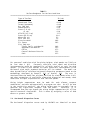
CONVERSION FACTORS
English to Metric System (SI) of Measurement
Quantity
English unit
Length
inches (in) or (")
Multiply by
To get metric equivalent
25.40
.02540
feet (ft) or (')
.3048
millimeters (mm)
meters (m)
meters (m)
miles (mi)
1.609
kilometers (km)
Area
square inches (in2)
square feet (ft2)
acres
6.432 x 10-4
.09290
.4047
square meters (m2)
square meters (m2)
hectares (ha)
Volume
gallons (gal)
cubic feet (ft3)
cubic yards (yd3)
3.785
.02832
.7646
liters (1)
cubic meters (m3)
cubic meters (m3)
Volume/Time
(Flow)
(l/s)
cubic feet per
28.317
liters
per
second
.06309
liters
per
second
second (ft3/s)
gallons per
(l/s)
minute (gal/min)
Mass
pounds (lb)
.4536
kilograms (kg)
Velocity
(m/s)
miles per hour (mph)
.4470
meters
per
second
feet per second (fps)
.3048
meters
per
second
feet per second squared
(ft/s2)
.3048
meters per second
squared (m/s2)
(m/s)
Acceleration
acceleration due to
force of gravity (G)
Weight
Density
pound per cubic
(lb/ft3)
Force
pounds (lbs)
kips (1000 lbs)
9.807
16.02
4.448
4.448
1
meters per second
squared (m/s2)
kilograms per cubic
meter (kg/m3)
newtons (N)
newtons (N)
Thermal
Energy
British thermal
unit (BTU)
Mechanical
Energy
foot-pounds(ft-lb)
foot-kips (ft-k)
1.356
1.356
joules (J)
joules (J)
Bending
Moment
or Torque
inch-pounds(in-lbs)
foot-pounds(ft-lbs)
.1130
1.356
newton-meters (Nm)
newton-meters (Nm)
Pressure
pounds per square
inch (psi)
pounds per quare
foot (psf)
Stress
(metre)1/2
Intensity
1055
6895
47.88
kips per square
1.0988
inch square root
inch (ksi (in)1/2)
joules (J)
pascals (Pa)
pascals (Pa)
mega
(MPa (m)1/2)
pounds per square
1.0988
kilo
(meter)1/2
inch square root
inch (psi (in)1/2)
(KPa (m)1/2)
Plane Angle degrees (E)
Temperature degrees
fahrenheit (F)
pascals
0.0175
radians (rad)
tF - 32 = tC degrees celsius (EC)
1.8
2
pascals
1. INTRODUCTION
CALINE3 is a third generation line source air quality model developed by
the California Department of Transportation. It is based on the Gaussian
diffusion equation and employs a mixing zone concept to characterize
pollutant dispersion over the roadway.
The purpose of the model is to assess air quality impacts near
transportation facilities in what is known as the microscale region. Given
source strength, meteorology, site geometry, and site characteristics, the
model can reliably predict pollutant concentrations for receptors located
within 150 meters of the roadway.
At present, the model can handle only
inert pollutants such as carbon monoxide, or particulates.
It is
anticipated that nitrogen dioxide predictive capabilities will be added to
the model within the next year.
Historically, the CALINE series of models required relatively minimal input
from the user. Spatial and temporal arrays of wind direction, wind speed
and diffusivity were not used by the models.
While CALINE3 has several
added inputs over its predecessor, CALINE2, it must still be considered an
extremely easy model to implement. More complex models are unnecessary for
most applications because of the uncertainties in estimating emission
factors and traffic volumes for future years.
As a predictive tool,
CALINE3 is well balanced in terms of the accuracy of state-of-the-art
emissions and traffic models, and represents a significant improvement over
CALINE2 in this respect.
The new model also possesses much greater
flexibility than CALINE2 at little cost to the user in terms of input
complexity.
This report should help the potential user of CALINE3 to understand and
apply the model. Users should become thoroughly familiar with the workings
of the model and, particularly, its limitations. This knowledge will aid
them in deciding when and how to use CALINE3.
Also, users should become
familiar with the response of the model to changes in various input
parameters.
This information is contained in the sensitivity analysis
portion of this report.
The results of a verification study using three separate data bases are
also contained in this report.
Dramatic improvements over CALINE2 are
shown, particularly for parallel winds and stable atmospheric conditions.
User instructions have been added along with several examples of CALINE3
applications which illustrate the variety of situations for which the model
can be used.
3
2.
BACKGROUND
In response to the National Environmental Policy Act of 1969, Caltrans
published its first line source dispersion model for inert gaseous
pollutants in 1972(1).
Model verification using the rudimentary field
observations then available was inconclusive.
In 1975, the original model was replaced by a second generation model,
CALINE2(2). The new model was able to compute concentrations for depressed
sections and for winds parallel to the highway alignment. The two models
were compared using 1973 CO bag sampling data from Los Angeles with CALINE2
proving superior.
Sometime after the dissemination of CALINE2, users began to report
suspiciously high predictions by the model for stable, parallel wind
conditions.
As a result, a more complete verification of the model was
undertaken by Caltrans using the 1974-75 Caltrans Los Angeles Data Base(3),
and the 1975 GM Sulfate Experiment Data Base(4). Comparison of predicted
and measured results showed that the predicted CO concentrations near the
roadway were two to five times greater than measured values for stable,
parallel wind conditions.
An independent study by Noll in 1977(5)
concluded that CALINE2 overpredicted for parallel winds by an average of
66% for all stabilities.
Overpredictions by CALINE2 for the stable, parallel wind case were
particularly significant.
This configuration was usually selected as the
worst case condition for predicting highway impact on air quality in the
microscale region.
Thus, beneficial highway projects might have been
delayed or cancelled on the basis of inaccurate results from CALINE2.
Inadequacies in the model also needed rectification.
The inability to
specify line source length and ground roughness severely limited the number
of situations in which the model could be properly applied.
Also,
predicting impacts from multiple sources required a series of runs with
varying receptor distances.
Such an unwieldy procedure could lead to
erroneous results.
In view of the inaccuracies and inadequacies of CALINE2, the model
assumptions and computational methods were reviewed with the idea of
revising the model.
Since, in some cases, the mathematical approach in
CALINE2 emphasized convenience and computational efficiency rather than a
rigorous treatment, it became apparent that revisions would not suffice and
a completely new model was needed. The new model would retain the Gaussian
formulation so that input requirements could be kept at a minimum.
However, the highway would be modeled as a series of finite line sources
positioned perpendicular to the wind direction, as opposed to the series of
virtual point sources used by CALINE2. Also, it was felt that new vertical
dispersion curves were needed.
The curves used by CALINE2 were modified
versions of Turner's curves(6).
These curves were derived for averaging
times of 10 minutes or less and extremely smooth terrain.
Both of these
4
factors contributed to the overpredictions for one-hour urban CO
concentrations.
Recent research by Caltrans(7) concluded that the amount
of vertical mixing near the roadway increased as wind speed decreased.
These findings were combined with more recently developed dispersion curves
published by Pasquill in 1974(8).
Adjustments for averaging time and
surface roughness also were included in the dispersion curve algorithms.
5
3.
CONCLUSIONS AND RECOMMENDATIONS
The comparisons of CALINE2 and CALINE3 made in the Verification Analysis
portion of this report clearly demonstrate the improved performance of the
new model.
It is concluded that the new algorithms contained in CALINE3
represent the dispersion process near highways in a more realistic way than
did CALINE2. In addition, the greater flexibility of the new model makes
it adaptable to many modeling applications not appropriate for CALINE2.
Finally, CALINE3 does not require additional computational time over
CALINE2 for equivalent applications. For these reasons, it is recommended
that CALINE3 replace CALINE2 as the official line source air quality model
used by Caltrans.
There are some aspects of CALINE3 on which further research is recommended:
1.
The residence time hypothesis needs to be studied for vehicle
speeds under 30 miles/hour.
2.
Verification of the model for intersection analysis must be
carried out.
3.
Validation of the deposition and settling velocity components
of the model is needed.
4.
Study of worst case meteorology as a function of land use and
geography is needed for more accurate evaluation of multi-hour
averages.
5.
N02 predictive capabilities must be added to the model and
verified.
6
4.
IMPLEMENTATION
This section was intentionally omitted in this abridged version to save
space. Nothing in the section is needed by the user to run the model. The
complete document is available from NTIS.
7
5.
5.1
MODEL DESCRIPTION
Gaussian Element Formulation
CALINE3 divides individual highway links into a series of elements from
which incremental concentrations are computed and then summed to form a
total concentration estimate for a particular receptor location.
The
receptor distance is measured along a perpendicular from the receptor to
the highway centerline.
The first element is formed at this point as a
square with sides equal to the highway width.
The lengths of subsequent
elements are described by the following formula:
EL = W*BASE(NE-1)
Where,
EL
W
NE
BASE
=
=
=
=
Element
Highway
Element
Element
PHI<20E,
20E#PHI<50E,
50E#PHI<70E,
70E#PHI
,
Where,
the
Length
Width
Number
Growth Factor
BASE=1.1
BASE=1.5
BASE=2.0
BASE=4.0
PHI = the angle between the wind direction and the direction of
roadway.
(Note: Capitalized variables shown in text are identical to those used in
the computer coding.)
Thus, as element resolution becomes less important with distance from the
receptor, elements become larger to permit efficiency in computation. The
choice of the element growth factor as a function of roadway-wind angle
(PHI) range represents a good compromise between accuracy and computational
efficiency.
Finer initial element resolution is unwarranted because the
vertical dispersion curves used by CALINE3 have been calibrated for the
link half-width (W2) distance from the element centerpoint.
Each element is modeled as an "equivalent" finite line source (EFLS)
positioned normal to the wind direction and centered at the element
midpoint.
A local x-y coordinate system aligned with the wind direction
and originating at the element midpoint is defined for each element. The
emissions occurring within an element are assumed to be released along the
EFLS representing the element. The emissions are then assumed to disperse
in a Gaussian manner downwind from the element. The length and orientation
of the EFLS are functions of the element size and the angle (PHI,φ) between
the average wind direction and highway alignment.
Values of PHI=0 or
PHI=90 degrees are altered within the program an insignificant amount to
avoid division by zero during the EFLS trigonometric computations.
8
In order to distribute emissions in an equitable manner, each element is
divided into five discrete sub-elements represented by corresponding
segments of the EFLS.
The use of five sub-elements yields reasonable
continuity to the discrete element approximation used by the model while
not excessively increasing the computational time. The source strength for
the segmented EFLS is modeled as a step function whose value depends on the
sub-element emissions.
The emission rate/unit area is assumed to be
uniform throughout the element for the purposes of computing this step
function.
The size and location of the sub-elements are a function of
element size and wind angle.
Downwind concentrations from the element are modeled using the crosswind
finite line source (FLS) Gaussian formulation.
5.2
Mixing Zone Model
CALINE3 treats the region directly over the highway as a zone of uniform
emissions and turbulence.
This is designated as the mixing zone, and is
defined as the region over the traveled way (traffic lanes - not including
shoulders) plus three meters on either side. The additional width accounts
for the initial horizontal dispersion imparted to pollutants by the vehicle
wake effect.
Within the mixing zone, the mechanical turbulence created by moving
vehicles and the thermal turbulence created by hot vehicle exhaust is
assumed to predominate near the ground. Evidence indicates that this is a
valid assumption for all but the most unstable atmospheric conditions(7).
Since traffic emissions are released near the ground level and model
accuracy is most important for neutral and stable atmospheric conditions,
it is reasonable to model initial vertical dispersion (SGZ1) as a function
of the turbulence within the mixing zone.
Analyses by Caltrans of the Stanford Research Institute(10) and General
Motors(4) data bases indicate that SGZ1 is insensitive to changes in
traffic volume and speed within the ranges of 4,000 to 8,000 vehicles/hr
and 30 to 60 mph(7).
This may be due in part to the offsetting effects of traffic speed and
volume.
Higher volumes increase thermal turbulence but reduce traffic
speed, thus reducing mechanical turbulence.
For the range of traffic
conditions cited, mixing zone turbulence may be considered a constant.
However, pollutant residence time within the mixing zone, as dictated by
the wind speed, significantly affects the amount of vertical mixing that
takes place within the zone. A distinct linear relationship between SGZ1
and residence time was exhibited by the two data bases studied.
CALINE3 arbitrarily defines mixing zone residence time as:
TR = W2/U
Where,
W2 = Highway half-width
9
U = wind speed
This definition is independent of wind angle and element size.
It
essentially provides a way of making the EFLS model compatible with the
actual two-dimensional emissions release within an element.
For oblique
winds and larger elements, the plume is assumed to be sufficiently
dispersed after traveling a distance of W2 such that the mixing zone
turbulence no longer predominates.
The equation used by CALINE3 to relate SGZ1 to TR is:
SGZ1 = 1.8 + 0.11* TR
(m)
(secs.)
This was derived from the General Motors Data Base. It is adjusted in the
model for averaging times other than 30 minutes by the following power
law(11):
SGZ1ATIM SGZ130* (ATIM/30)0.2
Where,
ATIM = Averaging time (minutes)
The value of SGZ1 is considered by CALINE3 to be independent of surface
roughness and atmospheric stability class. The user should note that SGZ1
accounts for all the enhanced dispersion over and immediately downwind of
the roadway.
Thus, the stability class used to run the model should be
representative of the upwind or ambient stability without any additional
modifications for traffic turbulence.
5.3
Vertical Dispersion Curves
The vertical dispersion curves used by CALINE3 are formed by using the
value of SGZ1 from the mixing zone model, and the value of σz at 10
kilometers (SZ10) as defined by Pasquill(8).
In effect, the power curve
approximation suggested by Pasquill is elevated near the highway by the
intense mixing zone turbulence. The significance of this added turbulence
to plume growth lessens with increased distance from the source, though, in
theory, it will never disappear.
Extrapolated σz curves measured out to
distances of 150 meters from the highway centerline under stable conditions
for both the GM and SRI data bases intersect the Pasquill curves at roughly
10 kilometers. Beyond this point the power curve approximation to the true
Pasquill curve, which is actually concave to the Rnx axis, becomes
increasingly inaccurate. Thus, the model should not be used for distances
greater than 10 kilometers. As will be seen in the sensitivity analysis,
contributions from elements greater than 10 kilometers from the receptor
are insignificant even under the most stable atmospheric conditions.
For a given set of meteorological conditions, surface roughness (Z0) and
averaging time (ATIM), CALINE3 uses the same vertical dispersion curve for
each element within a highway link. This is possible since SGZ1 is always
10
defined as occurring at a distance W2 downwind from the element
centerpoint. SZ10 is adjusted for Z0 and ATIM by the following power law
factors(11):
SZ10ATIM,Z0 = SZ10*(ATIM/3)0.2*(Z0/10)0.07
Where,
ATIM = Averaging time (minutes)
Z0 = Surface roughness (cm)
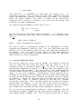
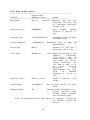
Table 1 contains recommended values of Z0 for representative land use
types(12).
The vertical dispersion of CO predicted by the model can be confined to a
shallow mixed layer by means of the conventional Gaussian multiple
reflection formulation(6).
This capability was included in the model to
allow for analysis of low traffic flow situations occurring during extended
nocturnal low level inversions. Surprisingly high 8 hour CO averages have
been measured under such conditions (13).
It is recommended for these cases that reliable, site specific field
measurements be made.
The following mixing height model proposed by
Benkley and Schulman (14) can then be used:
MIXH =
(0.185*U*k)/(Rn(Z/Z0)*f)
Where,
U = Wind speed (m/s)
Z = Height U measured at (m)
Z0 = Surface roughness (m)
k = von Karman constant (0.35)
f = Coriolis parameter
= 1.45 x 10 -4 cos θ (radians/sec)
θ = 90E - site latitude
11
TABLE 1
Surface Roughness for Various Land Uses
════════════════════════════════════════════════════════════════════
Type of Surface
Z0 (cm)
Smooth mud flats
Tarmac (pavement)
Dry lake bed
Smooth desert
Grass (5-6 cm)
(4 cm)
Alfalfa (15.2 cm)
Grass (60-70 cm)
Wheat (60 cm)
Corn (220 cm)
Citrus orchard
Fir forest
City land-use
Single family residential
Apartment residential
Office
Central Business District
Park
0.001
0.002
0.003
0.03
0.75
0.14
2.72
11.4
22.
74.
198.
283.
108.
370.
175.
321.
127.
════════════════════════════════════════════════════════════════════
For nocturnal conditions with low mixing heights, wind speeds are likely to
be less than 1 M/S.
Extremely sensitive wind speed and direction
instrumentation would be required for reliable results at such low wind
speeds. In order to use CALINE3 for these conditions, measurements of the
horizontal wind angle standard deviation will be needed.
The model can
then be modified to calculate horizontal dispersion parameters based on the
methodology developed by Pasquill (15) or Draxler (16)
The user is
cautioned that the model has not been verified for wind speeds below 1 M/S,
and that assumptions of negligible along-wind dispersion and steady state
conditions are open to question at such low wind speeds.
Mixing height computations must be made for each element receptor
combination, and thus add appreciably to program run time. As will be seen
in the sensitivity analysis, the mixing height must be extremely low to
generate any significant response from the model.
Therefore, it is
recommended that the user bypass the mixing height computations for all but
special nocturnal simulations. This is done by assigning a value of 1000
meters or greater to MIXH.
5.4
Horizontal Dispersion Curves
The horizontal dispersion curves used by CALINE3 are identical to those
12
used by Turner(6) except for averaging time and surface roughness power law
adjustments similar to those made for the vertical dispersion curves. The
model makes no corrections to the initial horizontal dispersion near the
roadway. The only roadway related alterations to the horizontal dispersion
curves occur indirectly by defining the highway width as the width of the
traveled way plus 3 meters on each side, and assuming uniform emissions
throughout the element.
If field measurements of the horizontal wind angle standard deviation are
available, site specific horizontal dispersion curves can be generated
using the methodology developed by Pasquill (15) or Draxler (16). CALINE3
can then be easily reprogrammed to incorporate the modified curves. This
approach is recommended whenever manpower and funding are available for
site monitoring.
5.5
Site Geometry
CALINE3 permits the specification of up to 20 links and 20 receptors within
an X-Y plane (not to be confused with the local x-y coordinate system
associated with each element). A link is defined as a straight segment of
roadway having a constant width, height, traffic volume, and vehicle
emission factor.
The location of the link is specified by its end point
coordinates. The location of a receptor is specified in terms of X, Y, Z
coordinates.
Thus, CALINE3 can be used to model multiple sources and
receptors, curved alignments, or roadway segments with varying emission
factors. The wind angle (BRG) is given in terms of an azimuth bearing (0
to 360E). If the Y-axis is aligned with due north then wind angle inputs to
the model will follow accepted meteorological convention (i.e., 90E
equivalent to a wind directly from the east).
The program automatically sums the contributions from each link to each
receptor. After this has been completed for all receptors, an ambient or
background value (AMB) assigned by the user is added. Surface roughness is
assumed to be reasonably uniform throughout the study area.
The
meteorological variables of atmospheric stability, wind speed, and wind
direction are also taken as constant over the study area. The user should
keep this assumption of horizontal homogeneity in mind when assigning link
lengths.
Assigning a 10 kilometer link over a region with a terrain
induced wind shift after the first 2 kilometers should be avoided.
A 2
kilometer link would be more appropriate.
The elements for each link are constructed as a function of receptor
location as described in Section 5.1. This scheme assures that the finest
element resolution within a link will occur at the point closest to the
receptor.
An imaginary displacement of the receptor in the direction of
the wind is used by CALINE3 to determine whether the receptor is upwind or
downwind from the link.
For each highway link specified, CALINE3 requires an input for highway
width (W) and height (H).
The width is defined as the width of the
13
traveled way (traffic lanes only) plus 3 meters on each side. This 3 meter
allowance accounts for the wake-induced horizontal plume dispersion behind
a moving vehicle. The height is defined as the vertical distance above or
below the local ground level or datum. CALINE3 should not be used in areas
where the terrain in the vicinity of the highway is uneven enough to cause
major spatial variability in the meteorology. Also, the model should not
be used for links with values of H greater than 10 meters or less than -10
meters.
Elevated highway sections may be of either the fill or bridge type. For a
bridge, air flows above and below the source in a relatively undisturbed
manner. This sort of uniform flow with respect to height is an assumption
of the Gaussian formulation.
For bridge sections, H is specified as the
height of the roadway above the surrounding terrain.
For fill sections,
however, the model automatically sets H to zero. This assumes that the air
flow streamlines follow the terrain in an undisturbed manner. Given a 2:1
fill slope (effectively made more gradual as the air flow strikes the
highway at shallower horizontal wind angles) and stable atmospheric
conditions (suppressing turbulence induced by surface irregularities), this
is a reasonable assumption to make (17).
For depressed sections greater than 1.5 meters deep, CALINE3 increases the
residence time within the mixing zone by the following empirically derived
factor based on Los Angeles data(3):
DSTR = 0.72* ABS(H)0.83
This leads to a higher initial vertical dispersion parameter (SGZ1) at the
edge of the highway.
The increased residence time, characterized in the
model as a lower average wind speed, yields extremely high concentrations
within the mixing zone.
The wind speed is linearly adjusted back to the
ambient value at a distance of 3*H downwind from the edge of the mixing
zone.
By this point the effect of the higher value for SGZ1 dominates,
yielding lower concentrations than an equivalent at-grade section.
For depressed sections, the model is patterned after the behavior observed
at the Los Angeles depressed section site studied by Caltrans(3). Compared
to equivalent at-grade and elevated sites, higher initial vertical
dispersion
was
occurring
simultaneously
with
higher
mixing
zone
concentrations. It was concluded that channeling and eddying effects were
effectively decreasing the rate of pollutant transport out of the depressed
section mixing zone.
Lower concentrations downwind of the highway were
attributed to the more extensive vertical mixing occurring within the
mixing zone.
Consequently, the model yields higher values for
concentrations within or close to the mixing zone, and somewhat lower
values than would be obtained for an at-grade section for downwind
receptors. Except for these adjustments, CALINE3 treats depressed sections
computationally by the same as at-grade sections.
It has been suggested that the model could be used for evaluating parking
lot impacts.
If the user wishes to run the model to simulate dispersion
14
from a parking lot, it is recommended that SGZ1 be kept constant at 1
meter, and that the mixing zone width not be increased by 3 meters on each
side as in the normal free flow situation. This is because the slow moving
vehicles within a parking lot will impart much less initial dispersion to
their exhaust gases.
5.6
Deposition and Settling Velocity
Deposition velocity (VD) is a measure of the rate at which a pollutant can
be adsorbed or assimilated by a surface.
It involves a molecular, not
turbulent, diffusive process through the laminar sublayer covering the
surface. Settling velocity (VS) is the rate at which a particle falls with
respect to its immediate surroundings. It is an actual physical velocity
of the particle in the downward direction. For most situations, a class of
particles with an assigned settling velocity will also be assigned the same
deposition velocity.
CALINE3 contains a method by which predicted concentrations may be adjusted
for pollutant deposition and settling. This procedure, developed by Ermak
(18), is fully compatible with the Gaussian formulation of CALINE3.
It
allows the model to include such factors as the settling rate of lead
particulates near roadways (l9) or dust transport from unpaved roads.
A
recent review paper by McMahon and Denison (20) on deposition parameters
provides an excellent reference.
Most studies have indicated that CO depositing is negligible.
In this
case, both deposition and settling velocity adjustments can be easily
bypassed in the model by assigning values of 0 to VD and VS.
15
6.
SENSITIVITY ANALYSIS
A sensitivity analysis for CALINE3 has been omitted from this abridged
document to save space. It is included in the complete document which is
available from NTIS.
16
7. MODEL VERIFICATION
The Model Verification Chapter has been omitted from this abridged document
to save space. It is included in the complete document which is available
from NTIS.
17
8.
8.1
USER INSTRUCTIONS
Restrictions and Limitations
8.1.1
Core requirements:
approximately 60K.
8.1.2 CALINE3 can process a maximum of 20 links per job. For each link,
the following must remain constant: The section type (TYP$), the source
height (HL), the mixing zone width (WL), the traffic volume (VPHL), and the
emission factor (EFL). If for any reason one of the variables changes, it
must be accounted for by a different link or an averaged value.
In the
case in which two links are parallel and identical, the two links may be
considered as one with mixing zone width equal to the sum of the two
traveled way widths plus the edge-to-edge median width plus 6 meters. The
median width may not exceed 10 meters.
8.1.3
CALINE3 can process a maximum of 20 receptors per job.
8.1.4
For any job, CALINE3 can process an unlimited number of
8.1.5
In setting up link dimensions, the link length should always be
greater than the link width.
18
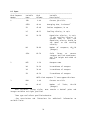
8.1.6 Input variable limits:
────────────────────────────────────────────────────────────────────
Suggested and
Variable
Mandatory Limits
Reason
────────────────────────────────────────────────────────────────────
Wind Speed
U$1 m/s
Gaussian assumption; with U$1 m/s,
along-wind diffusion can
be considered negligible
relative to U.
Wind Direction
0E#BRG#360E
Wind
azimuth
bearing
relative to positive Yaxis.
Averaging Time
3 min<ATIM<120 min
Reasonable limits of power
law approximation.
Surface Roughness
3 cm#Z0#400 cm
Mixing Zone
W$10 m
Link Length
W#LL#10 km
Stability Class
CLAS=1,2,3,4,5,6
Source Height
-10 m#H#10 m
Not
Receptor Height
Z$O
Gaussian plume reflected at airsurface interface; model
assumes
plume
transport
over horizontal plane.
Reasonable limits of
approximation.
power
law
Minimum of 1 lane plus 3
meters per side of link.
Link length, as defined by link
endpoint
coordinates
(Xl,Yl,X2,Y2),
must
be
greater than or equal to
link
width
for
correct
element
resolution,
and
less than or equal to 10
km
since
vertical
dispersion
curve
approximations
are
only
valid
for
downwind
distances of 10 km or
less.
Pasquill
scheme.
verified
range.
stability
outside
of
class
given
NOTE: For depressed sections Z$H (where H is negative) is permitted
for receptors within the
section.
19
────────────────────────────────────────────────────────────────────
8.1.7
The model should not be used in areas where the terrain in the
vicinity of the highway is sufficiently rugged to cause significant spatial
variability in the local meteorology.
8.1.8 The model should not be used for streets within a central business
district where the so-called street canyon effect is significant.
8.2
Grid Orientation
CALINE3 uses a combination of the X-Y Cartesian coordinate system and the
standard compass system to establish coordinate locations and link
geometry.
The standard, 360E compass is overlaid onto the X-Y coordinate
plane such that north corresponds to the +Y direction and east corresponds
to the +X direction. Wind angles (BRG) are measured as the azimuth bearing
of the direction from which the wind is coming (i.e., BRG = 270E for a wind
from the west). Coordinates, link height and link width may be assigned in
any consistent length units. The user must input a scale factor (SCAL) to
convert the chosen units to meters (SCAL=1. if coordinates and link height
and width are input in meters).
The X-Y grid and compass systems are combined into a single system and may
be used with north representing true or magnetic north or an assumed north.
In either case, once north has been chosen, all angles and X-Y pairs must
be consistently assigned. Negative coordinates are permitted.
20
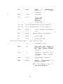
8.3 Input
───────────────────────────────────────────────────────────────────────
Card Sequence
Variable
Card
Variable
Number
Name
Columns
Description*
───────────────────────────────────────────────────────────────────────
1
JOB
1-40
Current job title**
2
ATIM
41-44
Averaging time, in minutes***
Z0
45-48
Surface roughness, in cm
VS
49-53
Settling velocity, in cm/s
VD
54-58
Deposition velocity, in cm/s;
if the settling velocity is
greater
than
0
cm/s,
the
deposition velocity should be
set equal to the settling
velocity.
NR
59-60
Number of
(Integer)
SCAL
61-70
Scale
factor
to
convert
receptor and link coordinates,
and link height and width to
meters.
RCP
1-20
XR
21-30
X-coordinate of receptor
YR
31-40
Y-coordinate of receptor
ZR
41-50
Z-coordinate of receptor
receptors;
NRmax=20
Receptor name
NOTE: Card sequence "2" must appear NR times.
3
RUN
1-40
NL
41-43
Current run title
Number
of
(Integer)
Real variables, except titles,
integer variables are right justified.
*
must
contain
a
links;
decimal
NLmax=20
point
and
Data type real unless specified otherwise.
**
See restrictions
variable limits.
***
and
limitations
21
for
additional
information
on
4
NM
44-46
LNK
1-20
TYP
21-22
XLl, YLl
23-29, 30-36 Coordinates of link endpoint 1
XL2, YL2
37-43, 44-50 Coordinates of link endpoint 2
VPHL
51-58
EFL
59-62
HL
63-66
Source height
WL
67-70
Mixing zone width
NOTE: Card sequence number "4"
5
Number
of
conditions;
(Integer)
meteorological
no
maximum
Link title
Section type
AJ=At-Grade
FL=Fill
BR=Bridge
DP=Depressed
Traffic volume in vehicles per
hour
Emission factor, in grams/mile
must appear NL times.
U
1-3
Wind speed, in m/s
BRG
4-7
Wind angle with respect to
positive Y-axis in degrees;
may
range
between
0E-360E,
inclusive.
CLAS
8
MIXH
9-14
Mixing height, in meters
AMB
15-18
Ambient
concentration
pollutant, in ppm
Atmospheric
in numeric
(Integer)
stability class,
format (1-6=A-F)
NOTE: Card sequence number
must appear NM times.
22
of
"5"
8.4
Output
Output for CALINE3 consists of printed listings containing a summary of all
input variables and model results. The input variables are separated into
site, link and receptor variables. Model results of CO concentration are
given in parts per million (ppm) for each receptor-link combination, and
are totaled (including ambient) for each receptor.
A separate page of
output is generated for each meteorological condition (three-page output
format is used when NL exceeds 10).
Other inert gaseous pollutants (such as SF6 tracer) may be run by changing
the molecular weight variable (MOWT) within the program to the appropriate
value, and modifying the output headings. Similarly, to run the model for
particulates, set FPPM=1 and again modify the headings. Results will be in
units of Fg/m3.
For both cases, the fixed point format for the output
should be modified to handle the range of results expected.
Jobs may be run consecutively, with a new series of pages being started for
each job. A brief data edit is executed for each job run. If an error is
found, a diagnostic is printed and program execution ends.
8.5
Examples
Four examples have been prepared to assist the user in understanding the
model's capabilities.
Each example demonstrates several important
characteristics of the model.
The user should note that the emission
factors quoted in these examples are not rigorously derived values.
Input data for all four examples are included in the file named
CALINE3.EXP. The resulting output is contained in CALINE3.LST. Below is
an abbreviated description of the four examples.
A more complete
description can be found in the complete document which is available from
MTIS.
8.5.1
Example One - Single Link
Example One is a simple illustration of a single link with one receptor
located near the downwind edge of the highway. The purpose of this example
is to show how the model handles links which are identical in every way
except for their section type and source height.
The link runs in a north-south direction and is 10,000 meters long.
The
vehicle volume (VPH) is 7500 vehicles/hour, the emission factor (EF) is 30
grams/mile and the mixing zone width (W) is 30 meters. The site variables
used are an averaging time (ATIM) of 60 minutes, an atmospheric stability
(CLAS) of 6(F), deposition and settling velocities (VD,VS, respectively) of
0 cm/second, an ambient CO concentration (AMB) of 3.0 ppm, and a surface
roughness (ZO) of 10 cm. The value for the surface roughness of 10 cm was
chosen because the link is assumed to be located in a flat, rural area
composed mainly of open fields.
The meteorological conditions of wind
23
speed (U) and wind angle (BRG) are 1 m/s and 270 degrees, respectively.
The 270 degree wind angle puts the direction of the wind perpendicular to
the link (crosswind) and from the west. The receptor is located 30 meters
east of the highway centerline at a "nose height" of 1.8 meters.
For case one, the link is defined as an at-grade type (TYP=AG, H=0). For
this configuration, the model calculates a CO concentration of 7.6 ppm.
This includes the 3.0 ppm ambient value shown under site variables.
Cases two and four involve elevated links. Each link is assigned a height
of 5 meters above the datum, but for case two the link is defined as a
bridge section (TYP=BR), while in case four it is considered a fill section
(TYP=FL).
The resulting CO concentrations are 6.2 ppm for the "bridge"
link and 7.6 ppm for the "fill" link. The difference in concentration is
due to the method in which contributions from the "bridge" and "fill" links
are calculated. For the "bridge" link in case two, it is assumed that the
wind is not only blowing over the link, but also underneath it. Thus, the
model can use the Gaussian adjustment for source height which assumes a
uniform vertical wind distribution both above and below the elevated
source. For the "fill" link, the model assumes that the wind streamlines
pass over the fill parallel to the ground.
Thus, the model treats case
four just as if it were an at-grade section.
For case three, the link is designated a depressed section (TYP=DP). All
conditions are identical to the previous cases except the source height.
CALINE3 increases the pollutant residence time within the mixing zone of a
depressed section, thus enhancing initial vertical dispersion.
This
accounts for the low CO concentration of 5.8 ppm predicted for case three.
8.5.2
Example Two - Rural Curved Alignment
Example two depicts the application of CALINE3 to a rural, curved
alignment.
Ten connecting links are used to model the highway.
The ten
links represent three straight sections, a 45E curve, and a 90E curve. The
90E curve is made up of five links, while the 45E curve is made up of only
two links. The finer resolution for the 90E curve is needed to obtain an
adequate approximation of the highway alignment for the nearby receptors.
For the given wind angle, the 45E curve will not contribute significantly to
any of the receptors, and thus is only divided up into two links.
The link conditions placed on this example are a constant vehicle volume of
8500 vehicles per hour and a constant emission factor of 30 grams/mile.
Also constant for all ten links are the at-grade source height, and mixing
zone width of 28 meters.
The two important site variables to note are the ambient concentration (3.0
ppm) and the surface roughness (50 cm).
The surface roughness of 50 cm
corresponds to assumed rolling, lightly wooded terrain. The model results,
which include the ambient concentration, appear to be consistent with what
would be expected under the wind angle of 45E.
24
8.5.3
Example Three - Urban Intersection
Example three represents a conventional urban intersection.
The user
should note that CALINE3 is not a street canyon model, and therefore should
not be used to model central business district intersections (i.e.,
surrounded by buildings of 4 stories or more).
Each street is divided into three links.
The intersection links are
assigned a much higher emission factor (100 grams/mile) than the
approaching links because of the vehicle idling and acceleration that
occurs at the intersection. In practice, a modal emissions model would be
used to predict a composite emission factor for the driving cycle
characteristic of the intersection being modeled.
Since the short
intersection links are separate from the longer approaching links, the
width of the short links can be made wider to include turn lanes. Thus,
the multiple link capability of CALINE3 allows the model to take into
account differences that exist along an arterial roadway.
The example is set in an urban location so that a surface roughness of 100
cm is used.
As in the preceding examples, a worst case 1 hour stability
class of F is assumed.
The model results include a 5.0 ppm ambient CO concentration.
8.5.4
Example Four - Urban Freeway
The final example is designed to show CALINE3's versatility. The example
consists of two primary links running east-west, 16 kilometers long. Set
in an urban location, the primary links carry traffic volumes of
approximately 10,000 vehicles/ hour, with an emission factor of 30
grams/mile. An on-ramp link is also included in the example. Because of
the constant acceleration occurring at the on-ramp, an emission factor of
150 grams/mile is used. As in Example three, this figure would be based on
a modal emissions model. Crossing the primary links are two bridge links
with traffic volumes of 4000 and 5000 vehicles/hour.
Twelve receptors are scattered all throughout the study
the model at wind angle increments around the compass,
identify the most critically affected receptors.
For
increments will be used. In practice, 10E increments are
area. By running
the user can then
this example, 90E
recommended.
With six links, twelve receptors, and four meteorological
CALINE3 is able to handle all situations in a single run.
25
conditions,
REFERENCES
1.
Beaton, J. L., et al, Mathematical Approach to Estimating Highway
Impact on Air Quality, Federal Highway Administration, FHWA-RD-72-36,
April 1972.
2.
Ward, C. E., et al, CALINE2 - An Improved Microscale Model for the
Diffusion of Air Pollutants from a Line Source, California Department
of Transportation (Caltrans), CA-DOT-TL-7218-1-76-23, November 1976.
3.
Bemis, G. R., et al, Air Pollution and Roadway Location, Design, and
Operation -Project Overview, Caltrans, FHWA-CA-TL-7080-77-25, September
1977.
4.
Cadle, S. H., et al, Results of the General Motors Sulfate Dispersion
Experiment, General Motors Research Laboratories, GMR-2107, March 1976.
5.
Noll, K. E., et al, "A Comparison of Three Highway Line Source
Dispersion Models", Atmospheric Environment, V. 12, pp 1323-1329, 1978.
6.
Turner,
D.
B.,
Workbook
of
Atmospheric
Environmental Protection Agency, 1970.
7.
Benson, P. E., and Squires, B. T., Validation of the CALINE2 Model
Using Other Data Bases, Caltrans, FHWA-CA-TL-79-09, May 1979.
8.
Pasquill, F., Atmospheric Diffusion, Wiley & Sons, 1974.
9.
Abramowitz, M., Handbook of Mathematical Functions, National Bureau of
Standards, 1968.
Dispersion
Estimates,
10. Dabberdt, W. F., Studies of Air Quality On And Near Highways, Project
2761, Stanford Research Institute, 1975.
11. Hanna, S. R., et al, "AMS Workshop on Stability Classification Schemes
and Sigma Curves - Summary of Recommendations", Bulletin American
Meteorological Society, V. 58, No. 12, pp 1305-1309, December 1977.
12. Myrup, L. O., and Ranzieri, A. J., A Consistent Scheme For Estimating
Diffusivities to be Used in Air Quality Models, Caltrans, FHWA-CA-TL7169-76-32, June 1976.
13. Remsburg, E. E., et al, "The Nocturnal Inversion and Its Effect on the
Dispersion of Carbon Monoxide at Ground Level in Hampton, Virginia",
Atmospheric Environment, V. 13, pp 443-447, 1979.
14. Benkley, C. W., and Schulman, L. L., "Estimating Hourly Mixing Depths
From Historical Meteorological Data", Journal of Applied Meteorology,
V. 18, pp 772-780, June 1979.
26
15. Pasquill,
Modeling,
1976.
F., Atmospheric Dispersion Parameters in Gaussian Plume
Environmental Protection Agency, EPA-600/4-76-0306, June
16. Draxler, R. R., "Determination of Atmospheric Diffusion Parameters",
Atmospheric Environment, V. 10, No. 2, pp 99-105, 1976.
17. Gloyne, R. W., "Some Characteristics of the Natural Wind and Their
Modification by Natural and Artificial Obstructions", Proceedings 3rd
International Congress of Biometeorology, Pergamon Press, 1964.
18. Ermak, D. L., "An Analytical Model for Air Pollutant Transport and
Deposition from a Point Source", Atmospheric Environment, V. 11, pp
231-237, 1977.
19. Little, P., and Wiffen, R. D., Emission and Deposition of Lead from
Motor Exhausts", Atmospheric Environment, V. 12, pp 1331-1341, 1978.
20. McMahon, T. A., and Denison, P. J., "Empirical Atmospheric Deposition
Parameters - A Survey", Atmospheric Environment, V. 13, pp 571-585,
1979.
21. Chock, D. P., The General Motors Sulfate Dispersion Experiment:
Assessment
of
the
EPA
Hiway
Model,
General
Motors
Research
Laboratories, GMR-2126, April 1976.
22. Golder, D. "Relations Among Stability Parameters in the Surface Layer",
Boundary-Layer Meteorology, V. 3, pp 47-58, 1972.
23. Munn, R. E., Descriptive Micrometeorology, Academic Press, p 161, 1966.
27