Download Hector user manual version 1.0

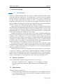
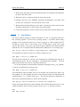
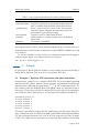
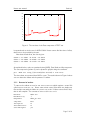
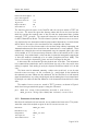
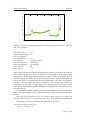
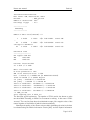
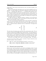
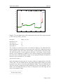
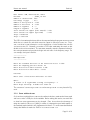
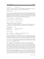
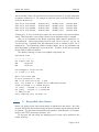
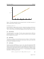
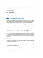
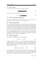
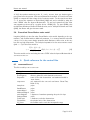
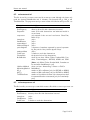
Hector user manual
version 1.0
Machiel Bos, Rui Fernandes and Luıisa Bastos
November 20, 2012
Contents
1 Introduction
1.1 How to cite Hector . . . . . . . . . . . . . . . . . . . . . . . . . . . .
1.2 Main features . . . . . . . . . . . . . . . . . . . . . . . . . . . . . . .
2
2
2
2 Installation
3
3 Tutorial
3.1 Example 1: Synthetic GPS time-series with spikes and offsets
3.1.1 Removal of outliers . . . . . . . . . . . . . . . . . .
3.1.2 Estimation of the linear trend . . . . . . . . . . . . .
3.1.3 Plotting the power spectral density . . . . . . . . . .
3.1.4 Some additional tests . . . . . . . . . . . . . . . . .
3.2 Example 2: A real GPS time-series with a lot of missing data
4 Acceptable data format
4.1 mom-format . . . .
4.2 enu-format . . . . .
4.3 neu-format . . . . .
4.4 rlrdata-format . . .
.
.
.
.
.
.
.
.
.
.
.
.
.
.
.
.
.
.
.
.
.
.
.
.
.
.
.
.
.
.
.
.
.
.
.
.
4
4
5
6
9
11
13
.
.
.
.
.
.
.
.
.
.
.
.
.
.
.
.
.
.
.
.
.
.
.
.
.
.
.
.
.
.
.
.
.
.
.
.
.
.
.
.
.
.
.
.
.
.
.
.
.
.
.
.
.
.
.
.
.
.
.
.
.
.
.
.
.
.
.
.
.
.
.
.
.
.
.
.
14
15
15
15
16
5 Implemented Noise Models
5.1 White noise . . . . . . . . . . . . . .
5.2 Power-law noise . . . . . . . . . . . .
5.3 Flicker noise and Random Walk noise
5.4 Power-law approximated . . . . . . . .
5.5 ARFIMA and ARMA . . . . . . . . .
5.6 Generalized Gauss Markov noise model
.
.
.
.
.
.
.
.
.
.
.
.
.
.
.
.
.
.
.
.
.
.
.
.
.
.
.
.
.
.
.
.
.
.
.
.
.
.
.
.
.
.
.
.
.
.
.
.
.
.
.
.
.
.
.
.
.
.
.
.
.
.
.
.
.
.
.
.
.
.
.
.
.
.
.
.
.
.
.
.
.
.
.
.
.
.
.
.
.
.
.
.
.
.
.
.
.
.
.
.
.
.
.
.
.
.
.
.
16
16
17
17
17
17
18
6 Quick reference for the control files
6.1 removeoutliers.ctl . . . . . . . . . . . . . . . . . . . . . . . . . . . . .
6.2 estimatetrend.ctl . . . . . . . . . . . . . . . . . . . . . . . . . . . . . .
6.3 estimatespectrum.ctl . . . . . . . . . . . . . . . . . . . . . . . . . . .
18
18
19
19
.
.
.
.
.
.
.
.
.
.
.
.
.
.
.
.
.
.
.
.
.
.
.
.
.
.
.
.
.
.
.
.
1
.
.
.
.
Hector user manual
Section 1
7 License and Copyright
1
20
Introduction
Hector is a software package that can be used to estimate the linear trend in timeseries with temporal corelated noise. Trend estimation is a common task in geophysical
research where one is interested in phenomena such as the increase in temperature,
sea level or GNSS derived station position over time. It is well known that in most
geophysical time-series the noise is correlated in time (Agnew, 1992; Beran, 1992) and
this has a significant influence on the accuracy by which the linear trend can be estimated.
Therefore, the use of a computer program such as Hector is advisable.
Hector assumes that the user knows what type of temporal correlated noise exists in
the observations and estimates both the linear trend and the parameters of the chosen
noise model using the Maximum Likelihood Estimation (MLE) method. Since for most
observations the choice of noise model can be found from literature or by looking at the
power spectral density, this is sufficient in most cases.
Instead of using Hector, one can also use the CATS software of Williams (2008) which
is a good and popular choice. In fact, Hector was written from scratch in C++ with the
objective to have a faster CATS. The reason is Hector is faster is that it accepts only
stationary noise, with constant noise properties, and this allows the use of fast matrices
operations. The obtained reduction in computation time is a factor of 10-100 compared
to CATS, see Bos et al. (2012). On the other hand, CATS has the advantage that it
offers a wider range of noise models. The choice is up to the user!
If the observations are non-stationary, then stationarity can be obtained by taking
the first difference of the data or using an approximation of the noise model as explained
by Bos et al. (2008, 2012) where also more information on the theoretical background
and more references can be found.
This manual starts in section 2 by explaining how to install Hector on your computer.
In section 3 a tutorial on using Hector is presented using two examples of analysing
synthetic GPS data with offsets and outliers and a real GPS data set. This is followed by
section 4 and 5 on acceptable data formats and implemented noise models respectively.
Finally, a quick reference of the parameters in the control files are presented in 6.
1.1
How to cite Hector
If you find the Hector program useful, please cite it in your work as:
Bos, M. S., Fernandes, R. M. S., Williams, S. D. P., and Bastos, L. (2012).
Fast Error Analysis of Continuous GNSS Observations with Missing Data.J.
Geod., ?:?–?
1.2
Main features
The main features of Hector are:
1. Correctly deals with missing data. No interpolation or zero padding of the data
nor an approximation of the covariance matrix is required (as long the noise is, or
has been made, stationary).
Page 2 of 21
Hector user manual
Section 2
2. Allows yearly, half-yearly and other periodic signals to be included in the estimation
process of the linear trend.
3. Allows the option to estimate offsets at given time epochs.
4. Includes power-law noise, ARFIMA, generalized Gauss-Markov and white noise
models. Any combination of these models can be made.
5. Allows taking the first difference of the data if power-law noise model is chosen
(including combination of white, flicker and random walk).
6. Comes with programs to remove outliers and to make power spectral density plots.
2
Installation
The hector software package is mainly intended to be run on computers with Unixlike operating systems. For the Linux operating system, a convenient debian binary
package can be downloaded from http://chbos.nl/hector. Hector requires the ATLAS (http://math-atlas.sourceforge.net/), FFTW3 (http://www.fftw.org/)
and the GSL (http://www.gnu.org/software/gsl/) libraries and these should be
installed first. On a computer with the Ubuntu linux distribution one can simply type:
sudo apt-get install libfftw3-3 libatlas3gf-base libgsl0ldbl
The installation procedure of hector on a 64-bit computer is now:
sudo dpkg -i hector_1.0_amd64.deb
This will put the binaries in /usr/bin, the documentation (including this manual) in
/usr/share/doc/hector and the examples in /usr/share/hector/examples. The man
pages of the binaries are stored in /usr/share/man/man1.
For 32-bit computers one should replace the debian package by hector_1.0_i386.deb.
To remove the 64 bit hector package, type:
sudo dpkg -r hector_1.0_amd64.deb
If this installation went successful, then one can skip the rest of this section and try out
the examples. For other systems the source code of Hector needs to be downloaded and
compiled using a C++ compiler such as g++. This will also require the installation of
some extra development libraries to obtain the header files:
sudo apt-get install libfftw3-dev libatlas-dev libgsl0-dev
If these extra three libraries have been installed in their default directories, then one can
compile the Hector source code by going to the hector-1.0/ directory and type:
make
sudo make install
Page 3 of 21
Hector user manual
Section 3
Table 1: List of programs provided by the Hector software package.
Name
Description
estimatetrend
Main program to estimate a linear trend.
estimatespectrum Program to estimate the power spectral density from the
data or residuals using the Welch periodogram method.
modelspectrum
Given a noise model and values of the noise parameters, this program computed the associated power spectral density for given frequency range.
removeoutliers
Program to remove outliers from the data.
date2mjd
Small program to convert calender date into Modified
Julian Date.
mjd2date
The inverse of date2MJD.
The programs, listed in Table 1, will by default be installed in the /usr/bin directory. If
another directory for the binaries is required the variable PREFIX in Makefile.inc needs
to be changed.
To run the examples one also need the Tcl scripting language and the gnuplot
plotting program. Again, on an Ubuntu machine one can type:
sudo apt-get install pgplot tcl
3
Tutorial
By going step by step through the analysis of some example data sets the working of
Hector will be explained. First, we look at some synthetic GPS data.
3.1
Example 1: Synthetic GPS time-series with spikes and offsets
In the directory examples/ex1 a data file called TEST.enu is stored which represents
some fictional GPS position data set. The file extension ‘enu’ stands for East-North-Up
and these three components are stored in the 2nd , 3rd and 4th column respectively. The
first column contain the Modified Julian Date (MJD) which is convenient format to
make plots. These data are stored in a simple ASCII text file and can be inspected by
any normal text editor. When doing so, one will detect some additional header lines:
#
#
#
#
#
#
sampling period 1.0
offset 50284.0 0
offset 50334.0 0
offset 50334.0 1
offset 50784.0 0
offset 51034.0 0
The first line just tells the program that the sampling period of the data is daily (T =1
day). Furthermore, there are offsets at the MJD epochs 50284, 50334, 50784 and 51034.
The last 0 indicates that these only occur in the East component (0=East, 1=North,
2=Up). If an offset occurs in more than one component, the header line for the offset
Page 4 of 21
Hector user manual
Section 3
140
’TEST.enu’ using (($1-51544)/365.25+2000):2
120
100
80
60
40
20
0
-20
-40
-60
1996
1996.5
1997
1997.5
1998
1998.5
1999
Figure 1: The raw data of the East component of TEST.enu.
is repeated such as is the case for MJD=50334. Hector cannot find the time of offset,
these have to be provided by the user.
After these header lines, the data is given:
50084.0 -17.88951 -21.47271 -19.38038
50085.0 -16.88599 -20.40868 -18.27968
50086.0 -16.84916 -20.31029 -18.14525
...
As explained before, each row contains the time (MJD), East, North and Up component.
The east component (column 2) can be plotted in gnuplot using the command:
plot ’TEST.enu’ using (($1-51544)/365.25+2000):2 with lines
The time values are converted from MJD to years. The result is shown in Figure 1 where
one can detect the offsets and the presence of outliers.
3.1.1
Removal of outliers
To remove the outliers we need to run removeoutliers which requires a control file
called removeoutliers.ctl. Hector uses various control files which are simple text
files and the rows with the labels can occur in any order. If Hector cannot find a label,
then it will complain. The contents of removeoutliers.ctl is:
DataFile
DataDirectory
OutputFile
component
interpolate
firstdifference
seasonalsignal
TEST.enu
./
TEST_pre.mom
East
no
no
yes
Page 5 of 21
Hector user manual
halfseasonalsignal
periodicsignals
estimateoffsets
IQ_factor
PhysicalUnit
ScaleFactor
Section 3
no
yes
3.0
mm
1.0
The first line gives the name of the DataFile with the raw data which is TEST.enu
in our case. The second line gives the directory where this file can be found and the
third live contains the required name of the file with the preprocessed data (outliers
removed): TEST_pre.mom. The output will always be in mom-format which stands
for MJD, Observations, Model. The last column is optional and since removeoutliers
only replaces the raw observations with the preprocessed observations, no third column
will be added. See section 4 for more details on the acceptable data format.
removeoutliers fits a linear trend to the raw data using ordinary least-sqares and
afterwards subtracts this linear trend from the observations to create residuals. These
residuals are ordered by size and the interquartile range is computed (this is the value
of the residual at 75% of the sorted array minus the value of the residual at 25% of the
sorted array). Any residual with a value less than 3 times this interquartile range below
or above the median is considered to be an outlier (Langbein and Bock, 2004). This
factor of 3 is set by the keyword IQ_factor and can be changed by the user.
In this control file one must also give the physical unit of the data. This information
is not essential but reminds the user to think about the unit of the data and if some
scaling is required. Such scaling is set by the keyword ScaleFactor which is 1.0 in this
case.
The linear trend is estimated assuming a white noise model and, as can be seen
from the removeoutliers.ctl file, a seasonal (i.e. yearly) signal is also included in
the estimation process. Offsets are also estimated. On the other hand, no half-seasonal
signal is estimated nor any other periodic signal and the missing data is not interpolated.
In principle one could take the first difference of the observations but this has not been
done.
The results of removeoutliers, stored in TEST_pre.mom, are shown in Figure 2
which have been generated with gnuplot using the command:
plot ’TEST.enu’ using (($1-51544)/365.25+2000):2 with lines,\
’TEST_pre.mom’ using (($1-51544)/365.25+2000):2 with lines
3.1.2
Estimation of the linear trend
Now that the outliers have been removed, we can estimate the linear trend. The parameters that control this analysis are given in the file estimatetrend.ctl:
DataFile
DataDirectory
OutputFile
interpolate
firstdifference
TEST_pre.mom
./
TEST_out.mom
no
no
Page 6 of 21
Hector user manual
Section 3
140
’TEST.enu’ using (($1-51544)/365.25+2000):2
’TEST_pre.mom’ using (($1-51544)/365.25+2000):2
120
100
80
60
40
20
0
-20
-40
-60
1996
1996.5
1997
1997.5
1998
1998.5
1999
Figure 2: The raw and preprocessed data of the East component stored in TEST.enu
and TEST_pre.mom.
seasonalsignal
halfseasonalsignal
periodicsignals
estimateoffsets
NoiseModels
LikelihoodMethod
MinimizingMethod
PhysicalUnit
ScaleFactor
yes
no
yes
Powerlaw White
AmmarGrag
NelderMead
mm
1.0
Again, there is the keyword DataFile which should be given by the name of the input file
which is TEST_pre.mom in this case because we are now going to use the preprocessed
observations. These preprocessed observations together with the estimated trend in
the third column, are written to the file name given after the keyword OutputFile. As
before, the data is not interpolated and the first difference of the data is not applied.
However, a seasonal signal and offsets are estimated. The chosen noise models are a
combination of power-law noise plus white noise. Alternatively we could have chosen
from: Flicker, RandomWalk, ARMA, ARFIMA or GGM (Generalized Gauss Markov) for
the noise models.
The numerical method for finding the maximum likelihood value is the Nelder &
Mead, also called Simplex, method. At the moment no other method has been implemented.
Note that if the ScaleFactor is not 1 in the file removeoutliers.ctl, then you
probably want to set it to 1 in estimatetrend.ctl to avoid applying the scaling twice.
The program estimatetrend shows the following on the screen:
***************************
Hector, version 1.0
Page 7 of 21
Hector user manual
Section 3
***************************
Data format: MJD, Observations, Model
Filename
: TEST_pre.mom
Number of observations: 1000
Percentage of gaps
: 10.7
---------------AmmarGrag
---------------Number of CPU’s used (threads) = 4
1
0.25000
0.17500
f()= 1736.224211
size=0.146
41
0.51029
0.38316
converged to minimum at
42
0.51033
0.38314
f()= 1724.982836
size=0.000
f()= 1724.982836
size=0.000
...
Likelihood value
-------------------min log(L)=-1724.983
AIC
=3453.966
BIC
=3463.555
Powerlaw: fraction=0.490
d = 0.3831 +/- 0.0868
White: fraction=0.5103
No noise parameters to show
STD of the innovation noise: 1.6190
bias : 0.831535 +/- 0.994658 mm (at MJD=50583.500000)
trend: 16.393336 +/- 0.687413 mm/year
cos yearly : 4.090394 +/- 0.280224 mm
sin yearly : -3.936342 +/- 0.285006 mm
offset at 50284.0000 : 24.493855 +/- 0.687678 mm
offset at 50334.0000 : -24.686144 +/- 0.750109 mm
offset at 50784.0000 : -39.755662 +/- 0.702739 mm
offset at 51034.0000 : 38.529800 +/- 0.724268 mm
--> TEST_out.mom
Total computing time: 4.00000 sec
The first lines are self explanatory. The number of CPU’s used is also shown to make
sure that Multi-Threading on Multi-Core Processors is working. In this case 4 CPU’s
are used. The next few lines show the minimization steps of the negative value of the
natural logaritm of the likelihood (which is thus maximised!).
Nowadays the quality of the chosen noise models in describing the noise in the data
is evaluated using the Akaike Information Criteria (AIC) and the Baysian Information
Page 8 of 21
Hector user manual
Section 3
Criteria (BIC). These values are shown below the value of the natural logarithm of the
Likelihood value.
Since we are using white and power-law noise, two noise parameters need to be
estimated. The first parameter (φ), determines the distribution of white and power-law
noise (φ = 1 represents 100% white noise, φ = 0 represents 100% power-law noise).
The second noise parameter is the slope of the power-law noise d. This is equal to 2α
and −2µ which is found in other papers on time-series analysis of GPS time-series. The
values of these two parameters need to be determined using the numerical minisation
scheme and their values during each step (42 steps are needed before convergence has
been reached) are shown in the output.
For white noise there is no additional parameter to estimate so, that is why there is
this line "No noise parameters to show" in the output in the white noise section. More
details on the noise models are given in section 5.
The rest of the lines show the estimated values of the model such as nominal bias
(offset of the whole time-series), linear trend and a seasonal signal. To get the most
accurate estimate of the linear trend, the linear trend in the design matrix has a zero
mean. To explain this better, assume that we have 5 observations. The design matrix
H looks like:


1 −2
1 −1




H = 1 0 
(1)


1 1 
1 2
The first column will estimate the nominal bias, the second the linear trend. The two
columns are orthogonal since HT H produces a diagonal matrix. Thus, the estimation of
the nominal bias is not influenced by the estimation of the linear trend which is beneficial
for the accuracy. It also means that the nominal bias corresponds to the value of the
model at the time at row 3 (half of the time-series). hector notes this time in the output
although in MJD. The program mjd2date can be used to convert in a calendar date.
Also shown in the output are the values of the estimated offsets. The results of
estimatetrend, stored in TEST_out.mom, are shown in Figure 3 which have been
generated in gnuplot with the command:
plot ’TEST.enu’ using (($1-51544)/365.25+2000):2 with lines,\
’TEST_out.mom’ using (($1-51544)/365.25+2000):2 with lines,\
’TEST_out.mom’ using (($1-51544)/365.25+2000):3 with lines
3.1.3
Plotting the power spectral density
We have used a power-law plus white noise model in our estimation process. To verify
if this is correct, it is good to make a power spectral density (PSD) plot of the residuals
(i.e. the difference between observations minus the estimated linear trend and additional
offsets and periodic signals). This can be done using the program estimatespectrum
which computes a Welch periodogram, stored in the file estimatespectrum.out. As
usual, the behaviour of this program is controlled by the file estimatespectrum.ctl:
Page 9 of 21
Hector user manual
Section 3
140
’TEST.enu’ using (($1-51544)/365.25+2000):2
’TEST_out.mom’ using (($1-51544)/365.25+2000):2
’TEST_out.mom’ using (($1-51544)/365.25+2000):3
120
100
80
60
40
20
0
-20
-40
-60
1996
1996.5
1997
1997.5
1998
1998.5
1999
Figure 3: The raw, filtered data and the estimated model of the East component stored
in TEST.enu and TEST_out.mom.
DataFile
DataDirectory
interpolate
firstdifference
ScaleFactor
TEST_out.mom
./
no
no
1.0
The contents of estimatespectrum.out is shown in Figure 4. By default the timeseries is devided into 4 parts by estimatespectrum. Since 50% overlap is used, there
are 7 segments in total and in this case the length of each segment is 250 data points.
The first and last 10% of each segment is smoothed to zero using a Parzen window
function. If more segments are required, to get a better averaging of the periodograms
but at the cost of a smaller frequency range, one can specify the number of divisions of
the data on the command line. For example:
estimatespectrum 8
which will divided the time-series into 8 pieces, creating 15 segments due to the 50%
overlap used. The area underneath the (one-sided) power spectral density plot should
be equal to the variance of the time-series (Buttkus, 2000). This area underneath the
PSD plot has been computed by simply assuming that each point represents a bar of
width 1/∆t and adding them all up. Next, it is important to note the begin and end
value of the frequency range.
---------------------EstimateSpectrum
----------------------
Page 10 of 21
Hector user manual
Section 3
Data format: MJD, Observations, Model
Filename
: ./TEST_out.mom
Number of observations: 1000
Percentage of gaps
: 10.7
Number of data points n : 1000
Number of data used
N : 1000
Number of segments
K : 7
Length of segments
L : 250
Total variance in signal (time domain): 3.297
Total variance in signal (spectrum)
: 3.123
freq0: 4.6296e-08
freq1: 5.7870e-06
The PSD of our estimated noise model can be computed using the program modelspectrum
which has no control file and which saves its output in modelspectrum.out. However, note that it gets information on the required set of noise models from the file
estimatetrend.ctl. Normally one makes a PSD after estimating the trend so this
should not be an inconvenience. The user must manually enter the requested values for
the noise parameters and provide the begin and end value of the frequency range. For
our example, the input looks like:
--------------ModelSpectrum
--------------Enter
Enter
Enter
Enter
the standard
the sampling
fraction for
fraction for
deviation of the innovation noise: 1.6190
period in hours: 24
model Powerlaw: 0.490
model White: 0.5103
Powerlaw:
Enter value of fractional difference d:0.3831
White:
1) Linear or 2) logarithmic scaling of frequency?: 2
Enter freq0 and freq1: 4.6296e-08 5.7870e-06
The contents of estimatespectrum.out and modelspectrum.out are plotted in Figure 4.
3.1.4
Some additional tests
So far we have explained how to remove the outliers in the data, estimate the linear trend
and how to make a PSD plot of the residuals. Before ending this section, we would like
to show how some parameters can be changed. First, let us show the advantage of
using the method of Bos et al. (2012) in terms of computation speed with respect to
the standard method which is also implemented in Hector. To use the standard method
change the likelihood method to FullCov in estimatetrend.ctl:
Page 11 of 21
Hector user manual
Section 3
0
Power (mm2/cpy)
10
observed
model
-1
10
-2
10
-3
10
0
1
10
10
2
10
Frequency (cpy)
Figure 4: The PSD of the residuals and used noise model.
LikelihoodMethod
FullCov
Running estimatetrend will now take about twice as long. Another method is ’Levinson’ which is also slower than AmmarGrag but was used by Bos et al. (2008). Note
that these three methods give the same answer as it should be. The Levinson method
becomes a lot faster if the data is interpolated. This can be achieved by altering the
keyword Interpolate in estimatetrend.ctl:
interpolate
yes
After running estimatetrend, which is now faster, we get:
Powerlaw: fraction=0.671
d = 0.3713 +/- 0.0810
White: fraction=0.3292
No noise parameters to show
STD of the innovation noise: 1.6077
bias : -0.318693 +/- 1.035911 mm (at MJD=50583.500000)
trend: 15.485505 +/- 0.724109 mm/year
One can see that linear interpolation of the missing data does not have a large effect
on the estimated noise parameters but the nomial bias and the linear trend are altered,
although still within the 95% confidence interval (2σ).
The spectral index is around 0.38, not too different from 0.5 which is the spectral
index for flicker noise. To investigate what the linear trend error is for flicker plus white
noise, we change the NoiseModels keyword to:
Page 12 of 21
Hector user manual
NoiseModels
Section 3
Flicker White
However, estimatetrend does not accept this right away because flicker noise is nonstationary. Therefore, we also need to set the keyword firstdifference:
firstdifference
yes
Now estimatetrend runs fine but note that there are now 20.42% missing data because
the missing data were artificially created at random times. Taking the first-difference thus
doubles the percentage of missing data. In real GPS time-series the effect is normally
less because of the presence of segments of missing data instead of only a set of single
missing data points. As a result, we obtain a larger trend uncertainty:
trend: 16.260990 +/- 4.542752 mm/year
If interpolation is used, then this result changes to:
trend: 15.467635 +/- 0.927564 mm/year
which is similar to the results obtained before.
Finally, one could use the approximation of the power-law covariance matrix as explained by Bos et al. (2012). This requires no interpolation and no first-difference:
interpolation
firstdifference
NoiseModels
TimeNoiseStart
no
no
PowerlawApprox White
1000.0
Now the result is:
bias : 0.870049 +/- 0.962471 mm (at MJD=50583.500000)
trend: 16.437759 +/- 0.721958 mm/year
There is no single set up which works best for all situations. Nevertheless, the AmmarGrag likelihood method (i.e. how the likelihood value is computed) is the fastest method
when the number of missing data is less than around 50%, otherwise the FullCov method
should be used. For GPS time-series the spectral index is normally around 0.5 (equal
to α = 1 or ν = −1) and we obtain in most case the best result with the noise model
combination "PowerlawApprox White".
3.2
Example 2: A real GPS time-series with a lot of missing data
GPS position time-series are normally given in a Cartesian reference frame with the origin
at the centre of the Earth, with the X and Y-axes lying in the equatorial plane and with
the X-axis passing through the Greenwich meridian. For plate tectonic research it is
more convenient to use the North, East and Up reference frame. This also separates the
Up component, which is normally noisier, from the North and East component. In the
directory examples/ex2 the script convert_sol_files.tcl performs this transformation. This script reads all filenames with the .sol extention in its directory and converts
each file from a Cartesian XYZ to a a geodetic East, North and Up reference frame
(enu-format, see section 4). This .sol data format is a special format and contains the
Page 13 of 21
Hector user manual
Section 4
date in the first column, the year-fraction in the second and the X, Y and Z component
in metres in columns 2 to 5. For example, the first four lines of the file PHLW.sol given
in the ex2 directory are:
2000-08-22
2000-08-23
2000-08-24
2000-08-25
2000.639344
2000.642077
2000.644809
2000.647541
4728141.4515
4728141.4479
4728141.4520
4728141.4585
2879662.3793
2879662.3730
2879662.3746
2879662.3813
3157146.8947
3157146.8923
3157146.8909
3157146.8986
Columns 6 to 11 are not shown but contain the autocovariance and cross-correlation
values. This information is not used by Hector and can therefore safely be omitted.
Here, we are interested in the North component which must be specified in removeoutliers.ctl. After preprocessing the data with removeoutliers, we can run
estimatetrend. A problem with this time-series is that it consists for 65% out of
missing data. The AmmarGrag likelihood method works, but is not particularly fast
when the number of missing data is more than 50%. Therefore, in this case one should
use the FullCov likelihood method.
The results of running estimatetrend (North component) are:
Likelihood value
-------------------min log(L)=-3157.577
AIC
=6319.154
BIC
=6329.770
PowerlawApprox: fraction=0.140
d = 0.5388 +/- 0.0617
White: fraction=0.8603
No noise parameters to show
STD of the innovation noise: 1.9233
bias : 113.351514 +/- 0.938288 mm (at MJD=53939.500000)
trend: 18.907049 +/- 0.143908 mm/year
cos yearly : 0.625495 +/- 0.211591 mm
sin yearly : 0.751631 +/- 0.238983 mm
--> PHLW_out.mom
Total computing time: 29.00000 sec
4
Acceptable data format
Hector can accept various data formats which are described in this section. All of the
are plain ASCII files and the time should always be increasing and the time step should
be constant. The data format is specified by the extension of the filename. For example,
the file name TEST.enu has the extension ’enu’.
For the mom and enu-format, the sampling period in days can be specified in the
header as follows:
Page 14 of 21
Hector user manual
Section 4
250
200
mm
150
100
50
0
-50
2000
2002
2004
2006
2008
2010
2012
2014
Years
Figure 5: The preprocessed data and the estimated model of the North component of
station PHLW, stored in PHLW_out.mom.
# sampling period 1.0
If this information is missing, then hector tries to estimate the sampling period from the
first few observations. The sampling periods it can detect automatically are: 0.5 hour,
1 hour, 1 day and 7 days. Note that this sampling period must always be given in days!
4.1
mom-format
This format expects 2 or 3 columns. The first column contains the time in MJD, the
second the Observations. The third column is optional and should contain the estimated
Model. Missing data are allowed.
4.2
enu-format
This format is similar to the mom-format but has four columns. The first column
contains the time in MJD, the second to the fourth column contain the East, North and
Up component. Missing data are allowed.
4.3
neu-format
This format is used by SOPAC (http://sopac.ucsd.edu/) and accepted by the CATS
software. The first column contains the time as year-fractions and columns two to four
contain the North, East and Up component in metres. Missing data are allowed. The unit
of these files is normally metres and it is convenient to convert these to millimetres using
the keyword ScaleFactor in removeoutliers.ctl. The year-fractions are converted
inside Hector to MJD using the formula:
M JD = f loor(365.25 ∗ (T − 1970) + 40587 + 0.1) − 0.5
(2)
Page 15 of 21
Hector user manual
Section 5
This implies that only sampling periods which are an integer multiple of 1 day are
acceptable. Hector can read the slightly different offset headers which are of the form,
see the CATS manual (Williams, 2008):
# offset 2003.45479 7
4.4
rlrdata-format
Hector can read PSMSL’s monthly data format, see http://www.psmsl.org/. To
create an evenly spaced data set inside Hector, each month is assumed to take exactly
30.4375 days, equal to 730.5 hours.
5
Implemented Noise Models
Hector can use various types of noise models and in addition, accepts various combinations of them with power-law plus white noise being the most popular for GPS time-series.
Williams (2008) wrote the covariance matrix C of this particular combination as:
C = σ 2 cos2 φ I + sin2 φ E(d)
(3)
where I is the unit matrix (equal to the covariance matrix for unit white noise) and E
the covariance matrix for power-law noise which depends on the spectral index d. The
distribution of the magnitudes of both noise models is controlled by the parameter φ.
The total variance of the noise is set by σ 2 . This has been generalized to:
C = σ 2 (φ1 (1 − φ2 ) . . . (1 − φN )E1 + (1 − φ1 )φ2 . . . (1 − φN )E2 +
(1 − φ1 )(1 − φ2 ) . . . φN EN +1 ) (4)
for N + 1 noise models. All φ-parameters vary between 0 and 1. As was noted in section
1, only stationary noise is accepted. This creates a Toeplitz covariance matrix and only
the first column of the covariance matrix needs to be stored. This column vector will be
denoted by γ.
5.1
White noise
For white noise the covariance matrix is just the unit matrix The first column of the
covariance matrix C, with σ = 1, is:
γi = 1
for i = 0
(5)
=0
i 6= 0
(6)
Its one-sided power spectrum density is:
S(f ) = 2
1
fs
(7)
where fs is the sampling frequency in Hz. If you integrate this from zero frequency to
the Nyquist frequency, you get the variance that is observed in the time-series, as it
should be.
Page 16 of 21
Hector user manual
5.2
Section 5
Power-law noise
For power-law noise the first column of the covariance matrix is:
γi =
Γ(d + i)Γ(1 − 2d)
Γ(d)Γ(1 + i − d)Γ(1 − d)
(8)
Its one-sided power spectrum density, with σ = 1, is:
S(f ) = 2
5.3
1
1
fs (2 sin(πf /fs ))2d
(9)
Flicker noise and Random Walk noise
Flicker noise and Random walk noise are simply two types of power-law noise where the
spectral index d has the fixed value of 0.5 and 1.0 respectively.
5.4
Power-law approximated
Bos et al. (2012) note that it is still not clear what causes the noise in GNSS time-series,
nor is it known when the noise started. This could be when the receiver was switched
on or since the launch of the GNSS satellites or some geophysical signal that has always
been present. They used this uncertainty to let the noise start at some arbitrary time
in the past. Since the noise is weakly stationary, after some time the covariance matrix
almost obtains a Toeplitz structure which means that fast matrix operations can be
used. This Toeplitz approximation can be chosen using the name ’PowerlawApprox’
after the keyword Noisemodels. In addition, one must specify the number of days before
the start of the observation when the noise is assumed to have started after the keyword
TimeNoiseStart. A value of 1000 is a good first guess.
5.5
ARFIMA and ARMA
The definition of the ARFIMA noise model is Sowell (1992):
Φ(L)(1 − L)d zt = Θ(L)ǫt
(10)
L is the backshift operator (Lxi = xi−1 ), zt is the residual at time t (observation minus
modelled signal) and ǫ is a white noise signal. In other words, Eq. (10) says that the
residuals in the observations can be produced by applying some transformations on a
white noise process. The operators Φ and Θ are defined as, see Hosking (1981) and
Brockwell and Davis (2002):
Φ(L) = 1 − φ1 L − φ2 L2 − . . . − φp Lp
2
q
Θ(L) = 1 + θ1 L + θ2 L + . . . + θq L
(11)
(12)
Note that the definition of the signs before the θ coefficients in Θ are sometimes inversed
in the literature. The value of the integers p and q are set by the keywords AR_p and
MA_q respectively in estimatetrend.ctl. It is advised to use values for p smaller than
5 to ensure that the MLE procedure always start with coefficients values for φ1 , . . . , φp
Page 17 of 21
Hector user manual
Section 6
of Φ(L) that produce stationary noise. If p and q are zero, then one obtains again a
pure power-law noise process. We have implemented the method of Doornik and Ooms
(2003) to compute the first column of the covariance matrix. For the special case when
d = 0, we use the equations of Zinde-Wash (1988) and can be selected by using the
name ’ARMA’ after the keyword Noisemodels. For sea level research the first order
auto-regressive noise model is a popular choice: ARMA(1,0). For pure ARMA noise
models faster Maximum Likelihood Methods exist, see for example Brockwell and Davis
(2002), but Hector will give the same result.
5.6
Generalized Gauss Markov noise model
Langbein (2004) took the first order Gauss Markov noise model depending on the parameter φ and modified with an additional parameter, d, to create power-law noise with
a slope of 2d in the power density spectrum which flattens to white noise at the very
low and very high frequencies. The analytical expression for the autocovariance vector
(with σ = 1) for this noise model is:
γi =
Γ(d + i)(1 − φ)i
2
2 F1 (d, d + i; 1 + i; (1 − φ) )
Γ(d)Γ(1 + i)
(13)
This noise model can be used using the name ’GGM’ after the keyword Noisemodels in
estimatetrend.ctl.
6
6.1
Quick reference for the control files
removeoutliers.ctl
This file is read by removeoutliers.
Keyword
DataFile
DataDirectory
OutputFile
component
interpolate
firstdifference
seasonalsignal
halfseasonalsignal
periodicsignals
estimateoffsets
ScaleFactor
PhysicalUnit
IQ_factor
Label(s)
name of file with observations
directory where file with observations is stored
name of file with observations and estimated model in
.mom format
only required for the .enu and .neu format. Select East,
North or Up
yes|no
yes|no
yes|no
yes|no
a sequence of numbers reprenting the period in days
yes|no
a number to scale the observations
the physical unit of the observations
the number used to scale the interquartile range
Page 18 of 21
Hector user manual
6.2
Section 7
estimatetrend.ctl
This file is read by estimatetrend and by modelspectrum although the latter only
reads the keyword NoiseModels and, if necessary, the keywords AR_p, MA_q and
TimeNoiseStart. The program modelspectrum creates a file called modelspectrum.out.
Keyword
DataFile
DataDirectory
OutputFile
component
interpolate
firstdifference
seasonalsignal
halfseasonalsignal
periodicsignals
estimateoffsets
ScaleFactor
PhysicalUnit
NoiseModels
LikelihoodMethod
MinimizingMethod
AR_p
MA_q
TimeNoiseStart
6.3
Label(s)
name of file with observations
directory where file with observations is stored
name of file with observations and estimated model in
.mom format
only required for the .enu and .neu format. Select East,
North or Up
yes|no
yes|no
yes|no
yes|no
a sequence of numbers, separated by spaced, representing the period of the periodic signals in days
yes|no
a number to scale the observations
the physical unit of the observations
chose any set from: White, Flicker, RandomWalk, Powerlaw, PowerlawApprox, ARFIMA, ARMA and GGM.
(Note: only White, Flicker, RandomWalk, Powerlaw can
be used when firstdifference=yes)
chose one from: AmmarGrag, Levinson or FullCov
NelderMead
number of AR coefficients (only for ARFIMA or ARMA)
number of MA coefficients (only for ARFIMA or ARMA)
number of days before the start of the observations when
it is assumed that the noise started (only for PowerlawApprox)
estimatespectrum.ctl
This file is read by estimatespectrum which creates a file called estimatespectrum.out.
Keyword
DataFile
DataDirectory
interpolate
firstdifference
ScaleFactor
Label(s)
name of file with observations
directory where file with observations is stored
yes|no
yes|no
a number to scale the observations
Page 19 of 21
Hector user manual
7
Section 7
License and Copyright
Hector is Copyright © 2012-1016 Machiel Bos, Rui Fernandes and Luísa Bastos.
Hector is free software; you can redistribute it and/or modify it under the terms of
the GNU General Public License as published by the Free Software Foundation; either
version 2 of the License, or (at your option) any later version.
This program is distributed in the hope that it will be useful, but WITHOUT ANY
WARRANTY; without even the implied warranty of MERCHANTABILITY or FITNESS
FOR A PARTICULAR PURPOSE. See the GNU General Public License for more details.
You should have received a copy of the GNU General Public License along with this
program; if not, write to the Free Software Foundation, Inc., 51 Franklin Street, Fifth
Floor, Boston, MA 02110-1301 USA You can also find the GPL on the GNU web site.
References
Agnew, D. C. (1992). The time-domain behaviour of power-law noises. Geophys. Res.
Letters, 19(4):333–336.
Beran, J. (1992). Statistical methods for data with long-range dependence. Statistical
Science, 7(4):404–416.
Bos, M. S., Fernandes, R. M. S., Williams, S. D. P., and Bastos, L. (2008). Fast error
analysis of continuous GPS observations. J. Geod., 82:157–166.
Bos, M. S., Fernandes, R. M. S., Williams, S. D. P., and Bastos, L. (2012). Fast Error
Analysis of Continuous GNSS Observations with Missing Data. J. Geod., ?:?–?
Brockwell, P. and Davis, R. A. (2002). Introduction to Time Series and Forecasting.
Springer-Verlag, New York, second edition edition.
Buttkus, B. (2000). Spectral Analysis and Filter Theory in Applied Geophysics. SpringerVerlag Berlin Heidelberg.
Doornik, J. A. and Ooms, M. (2003). Computational Aspects of Maximum Likelihood
Estimation of Autoregressive Fractionally Integrated Moving Average Models. Computational Statistics and Data Analysis, 42:333–348.
Hosking, J. R. M. (1981). Fractional differencing. Biometrika, 68:165–176.
Langbein, J. (2004). Noise in two-color electronic distance meter measurements revisited.
J. Geophys. Res., 109(B04406).
Langbein, J. and Bock, Y. (2004). High-rate real-time GPS network at Parkfield: Utility
for detecting fault slip and seismic displacements. Geophys. Res. Letters, 31:15.
Sowell, F. (1992). Maximum likelihood estimation of stationary univariate fractionally
integrated time series models. J. Econom., 53:165–188.
Williams, S. D. P. (2008). CATS : GPS coordinate time series analysis software. GPS
Solutions, 12(2):147–153.
Page 20 of 21
Hector user manual
Section 7
Zinde-Wash, V. (1988). Some Exact Formulae for Autoregressive Moving Average Processes. Econometric Theory, 4(3):384–402.
Page 21 of 21