Download The Workload Analyser Tool User Guide

The Workload Analyser Tool
User Guide
The Integrated Modelling Support Environment project
Maria Calzarossa
Lionel Mallet
Luisa Massari
Giuseppe Serazzi
R4.2 { 4 Version 1
June 1991
c University of Pavia 1991
Distribution level All IMSE project teams
Approved by
The IMSE Project The IMSE project is a collaborative research project supported by the
CEC as ESPRIT project no. 2143. It is being carried out by the following organisations :- BNR
Europe STL, Thomson CSF, Simulog A.S., University of Edinburgh, INRIA, IPK (Berlin),
University of Dortmund, University of Pavia, SINTEF (University of Trondheim), University of
Turin and University of Milan.
Contents
References
2
1 The Workload Analyser Tool
3
2 Getting started
6
3 The graphical interface
6
3.1 The \WAT Editor main window" . . . .
3.2 The Define button . . . . . . . . . . .
3.2.1 \List of format library" window .
3.2.2 \Format" window . . . . . . . .
3.2.3 \Variables" window . . . . . . .
3.2.4 Saving the specications . . . . .
3.3 The Load button . . . . . . . . . . . . .
3.4 The Run button . . . . . . . . . . . . . .
.
.
.
.
.
.
.
.
.
.
.
.
.
.
.
.
.
.
.
.
.
.
.
.
.
.
.
.
.
.
.
.
.
.
.
.
.
.
.
.
.
.
.
.
.
.
.
.
.
.
.
.
.
.
.
.
.
.
.
.
.
.
.
.
.
.
.
.
.
.
.
.
.
.
.
.
.
.
.
.
.
.
.
.
.
.
.
.
.
.
.
.
.
.
.
.
.
.
.
.
.
.
.
.
.
.
.
.
.
.
.
.
.
.
.
.
.
.
.
.
.
.
.
.
.
.
.
.
.
.
.
.
.
.
.
.
.
.
.
.
.
.
.
.
.
.
.
.
.
.
.
.
.
.
.
.
.
.
.
.
.
.
.
.
.
.
.
.
.
.
.
.
.
.
.
.
.
.
.
.
.
.
.
.
7
8
11
11
12
13
14
14
4 An example
15
Appendix
22
A Use of the components of the interface
22
A.1
A.2
A.3
A.4
A.5
A.6
A.7
A.8
Buttons . . . . . . . .
Menus . . . . . . . . .
Sum items . . . . . . .
Integer range items . .
String items . . . . . .
Filename string items
List items . . . . . . .
Resizing a window . .
.
.
.
.
.
.
.
.
.
.
.
.
.
.
.
.
.
.
.
.
.
.
.
.
.
.
.
.
.
.
.
.
.
.
.
.
.
.
.
.
.
.
.
.
.
.
.
.
.
.
.
.
.
.
.
.
.
.
.
.
.
.
.
.
.
.
.
.
.
.
.
.
.
.
.
.
.
.
.
.
.
.
.
.
.
.
.
.
.
.
.
.
.
.
.
.
.
.
.
.
.
.
.
.
.
.
.
.
.
.
.
.
.
.
.
.
.
.
.
.
.
.
.
.
.
.
.
.
.
.
.
.
.
.
.
.
.
.
.
.
.
.
.
.
.
.
.
.
.
.
.
.
.
.
.
.
.
.
.
.
.
.
.
.
.
.
.
.
.
.
.
.
.
.
.
.
.
.
.
.
.
.
.
.
.
.
.
.
.
.
.
.
.
.
.
.
.
.
.
.
.
.
.
.
.
.
.
.
.
.
.
.
.
.
.
.
.
.
.
.
.
.
.
.
.
.
.
.
.
.
.
.
.
.
.
.
.
.
.
.
.
.
.
.
.
.
.
.
.
.
.
.
.
.
.
.
.
.
.
.
.
.
.
.
22
22
24
24
25
25
26
27
References
1] Maria Calzarossa and Luisa Massari, Requirement Specications of the Workload Analyser
Tool. Document IMSE R4.2 { 1, University of Pavia, 1989
2] Maria Calzarossa, Luisa Massari and Giuseppe Serazzi, The Workload Analyser Tool - User
Interface. Document IMSE R4.2 { 2, University of Pavia, 1990
3] Maria Calzarossa, Luisa Massari and Giuseppe Serazzi, The Design of the Workload Analyser Tool. Document IMSE D4.2 { 1 Version 1, 1990
4] Andreas L. Opdahl and Vidar Vetdland, Evaluation of EXT and WAT design. Document
IMSE R6.6 { 6, SINTEF, 1990
5] Chris Uppal, Design of the IMSE SDMF. Document IMSE R2.2 { 3, STC Technology, 1990
2
1 The Workload Analyser Tool
Workload characterization, i.e., the quantitative description of the processing requests to a system, is a fundamental part of any type of performance evaluation study. Indeed, every time the
knowledge of the performance of a system is needed, the workload which produced these values
must be determined.
Since workloads are usually constituted by a large number of components and each component
is described by a tuple of parameters (variables), the amount of resulting data to be analyzed
is generally considerable.
The Workload Analyser Tool (WAT) can be used to derive a manageable and more compact
representation of the workload, in that it allows the construction of workload models whose
characterizing parameters can be used as input for either analytic and simulation system models.
WAT processes raw input data collected by means of the measurement tools and the routines
available on the target systems, and identies, by means of suitable statistical techniques, a set
of groups (classes) of components having homogeneous characteristics.
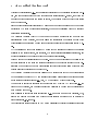
Figure 1 shows the overall structure of the tool. One of the main features of the design is the
modular structure of the tool the various operations of the procedure required for the construction of a workload model have been logically subdivided into seven steps where each step
performs specic operations on the input data.
The Workload Analyser Tool has been designed to be independent of the type of data streams
to be analyzed the input of WAT can consist of accounting les measured on systems running
under various operating systems (i.e., Unix, VME) as well as ASCII or binary les.
The user has to specify the structure of the records in the ASCII/BINARY input les, i.e., the
format of each variable, and has also to select the variables to be used for the description of
each workload component.
It is possibile to specify all these information (e.g., mnemonic names of the variables, type,
length) the rst time a certain type of input data is selected and store them in a library of
record structures, i.e., formats.
Another relevant feature included in WAT is the possibility of directly processing accounting
3
les measured on systems running under UNIX or VME operating systems. A lot of preliminary
work is required to convert such les in a \readable" format since, for eciency reasons, they
are usually stored in a \compressed" format not easily \decoded".
For saving disk space, the WAT can accept input from either disk or tape is given.
After the input description and the selection of the characterizing parameters of each workload
component, the \real" processing of workload data begins. The basic statistical descriptors, such
as, mean, variance, standard deviation, skewness, kurtosis, maximum and minimum values, are
provided.
A preliminary analysis of the input data, which includes application of various types of transformation, trimming of the outliers and sampling, is performed. All these operations are mainly
aimed towards the clustering analysis, which represents the core of the WAT since it allows the
construction of workload models and the identication of the input parameters for the corresponding system models.
4
external
world
WAT
raw data
?
step 1
input description
?
step 2
parameter selection
?
step 3
statistical analysis
-
?
step 4
transformations
-
?
step 5
outliers
?
step 6
sampling
-
?
step 7
cluster analysis
?
workload model
?
modelling tools
Figure 1: Overall structure of the Workload Analyser Tool.
5
2 Getting started
Three dierent execution modes are supported by the Workload Analyser Tool. The user can
choose to use the graphical interface to prepare the input specications for a batch run or to
directly run the tool, either in a batch or an interactive mode.
The WAT can be invoked as follows:
wat:
interactive mode the WAT starts without any graphical interface and the logical
subdivision of the tool in the seven steps presented in Sect. 1 is maintained
wat -h: help on-line general information about the WAT are displayed
wat -b <filename>: batch mode the WAT starts in batch mode without any graphical
interface. <filename> is the name of the le containing the specications of all the
operations to be performed on the input data. The le has to be previously created in a
graphical mode
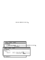
wat -i: graphical mode the graphical interface of WAT opens the \WAT Editor main
window" (see Fig. 2) which gives the user various options. As we will clarify in the
following section, the user can either dene a new set of specications, load an existing
one, or run WAT in batch mode.
Figure 2: Main menu of the Workload Analyser Tool graphical interface.
3 The graphical interface
The graphical interface - WAT Editor - (running wat with the \-i" option) allows the user to
select the various operations to be performed on the input data. All these specications will be
6
stored in a le which can be used for a batch execution of the WAT. Let us remark that the
same specications can be selected step by step in an interactive mode.
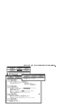
Figure 3 shows an example of a WAT Editor session.
Figure 3: Example of WAT Editor session.
Note that the current version of the graphical interface runs on Sun computers and is built on
top of the SDMF 5]. The basic management operations associated to the components of the
interface can be found in Appendix A.
3.1 The \WAT Editor main window"
The interface starts by displaying a window labelled \WAT Editor main window" (see Fig. 2).
This window contains six buttons:
Done
Save
Abort
Define
7
Load
Run
No action is associated to the Save button. Both the Done and the Abort buttons allow the
user to quit and leave the interface. The operations associated to the remaining buttons will be
explained in the following sections.
An Help button is also provided. It allows the user to open a window containing a few basic
information about the \WAT Editor main window" and, eventually, to store new information/comments.
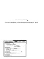
3.2 The Define button
To dene a new set of specications, the user needs to select the Define button in the \WAT
Editor main window". A new window, called \WAT Editor window", is opened (see Fig. 4).
Figure 4: The \WAT Editor window".
This window, which gathers a few preliminary information, is logically subdivided in four
sections related to the Input Specifications, the Control Specifications, the Display
Specifications and the Output Specifications, respectively. Each section has its own help
on line which is available through the Help button.
8
Input Specifications
In this section the user can dene all the information related to how the tool has to manage the
measurement data (input le) before their statistical analysis (step 1 to 4 of the WAT - see Fig.
1). The possible choices are:
List of format library: the user can list the contents of his local library of ASCII/BINARY
formats. A specic window is opened (see \List of format library" window below - subform
button)
File type: it allows the user to specify the format of the input data (i.e., the organization
of the data in the input le) this sum item gathers the following standard formats: UNIX
accounting, VME accounting, user pre-dened formats (found in the library located in the
working directory and displayed by name) and new ASCII/BINARY formats.
Let us examine in details the various options:
1. accounting format: the user has the following possibilities within the sum item
File:
{
disk:
the le is stored on disk the name of the le containing the data (lename
string item Filename) must be specied
{ tape: the le is stored on a tape the user has to specify the name of the device
driver associated to the tape (lename string item Drive)
2. user pre-dened format: the name of the le containing the data (lename string
item Filename) is required
3. new ASCII/BINARY format: the user has to specify the name of the le containing
the measurement data (lename string item Filename). The structure of the le, i.e.,
the format, is dened in the \Format" window (see the \Format" subform).
In all the three cases, the user will also have to specify the information of the parameters he
wants to analyze (see the \Variables" subform).
9
Control Specifications
This section is concerned with the information related to the analysis of the measurement data,
namely:
Percentile of outliers: the percentile of the distribution of each variable for trimming
of the outliers is specied (integer range item)
Random Sample: the user can select a random sample (sum item) an integer range item
is displayed to choose the percentage of data of the sample
Number of clusters:
an integer range item allows the user to specify the number of
clusters he wants to obtain with the cluster analysis
Overall transformation: a sum item for the selection of the transformation to be applied
to all the variables in order to scale them to the same range before the cluster analysis.
Display Specifications
This section deals with:
Display of Statistical Information: the user can select to display the statistical information during the analysis of the data (sum item)
Display of Cluster Distributions: the distributions of the variables can be displayed
for the entire population or for each of the clusters.
Output Specifications
This sections deals with:
Output file: a lename string item containing the name of the le where the WAT will
save the results of the cluster analysis
Output specifications: this feature is not yet implemented.
10
Figure 5: The \List of format library" window.
3.2.1 \List of format library" window
The user can list the contents of the local library one format at a time. The name of the format
he wants to display has to be selected through the rst sum item.
3.2.2 \Format" window
Figure 6: The \Format" window.
This window contains its own help, available, as usual, through the Help button located at the
top of the window, and a few items to dene the specic format, namely:
Format Name: name of the format (string item)
Formatted: a sum item for the specication of the type of record structure, i.e., formatted
(ASCII), or unformatted (binary)
Format: list of the format of each variable. Depending on the previous choice (formatted or
unformatted), the user will have to ll the Format list item with the name of each variable
11
(string item), its type, (sum item), i.e., real or integer, and, in the case of formatted
records, with the length (i.e., number of digits) of eld associated to the variable itself
(integer range items).
All the specications are saved by selecting either the Done or Save buttons. Alternatively, they
can be discarded by selecting the Abort button.
WARNING
The save operation does not write permanently the format information in the local library. This
operation simply means \keep the information for the current session". The format will be saved
in the local library when the user will save the whole specications in the \WAT Editor window"
(see Sect. 3.2.4).
3.2.3 \Variables" window
Figure 7: The \Variables" window.
This window contains its own help, available, as usual, through the Help button, and a list item
to specify the variables the user wants to analyze and how to perform this analysis.
This list consists of four components:
Name: name of the variable this item is a string item in case of a new ASCII/BINARY
format or a sum item otherwise. Let us remark that for a new ASCII/BINARY format
the name must correspond to a name of the variable given in the format denition
New: to associate a new name to the variable (string item)
12
Transform.: to specify the transformation(s) to be applied to each variable (sum item)
Outliers: to specify if the user wants to remove the outliers for a specic variable (sum
item).
The Done or Save buttons and the
selections, respectively.
Abort
button allow the user to save and discard all the
3.2.4 Saving the specications
To permanently save the whole specications, the user has to click either the Save or Done
buttons. The operation associated to these buttons consists of displaying a \Save description in
le..." window (see Fig. 8), where the name of the le containing the specications has to be
given.
Figure 8: The \Save description in le..." window.
The save operation can be interrupted by clicking the Abort button in the \Save description in
le..." window.
The Abort button of the \WAT Editor window" allows the user to close the window.
Note that the specications are not automatically saved. It is necessary to explicitly require a
save operation before closing the \WAT Editor window".
13
3.3 The Load button
To load an existing set of specications, the user needs to select the Load operation in the \WAT
Editor main window" and provide in the \Load description from le..." window (see Fig. 9)
the name of the le containing the specications. The matching of the lename is performed
by clicking the Done or the Save button. The set of specications is displayed in a \WAT
Editor window" as described in section 3.2. The user can refer to this section for the available
operations.
Figure 9: The \Load description from le..." window.
3.4 The Run button
The user can run the WAT in batch mode from the interface by selecting the Run operation in
the \WAT Editor main window". It is necessary to provide in the \Run WAT with batch le..."
window (see Fig. 10) the name of the le containing the specications. The matching of the
lename is performed by clicking the Done or the Save button. The execution of the WAT starts
in background mode.
Figure 10: The \Run WAT with batch le..." window.
14
4 An example
In order to make clearer the description of the graphical interface of the WAT, we will present
the use of the tool on a real set of data.
The problem we approach in this example is the analysis of measurements collected on an
Ethernet local area network. The data refers to the packets sent to the network from either
workstations and disk servers. Among the various information describing each packet we have
selected two parameters:
packet length (in bytes),
interarrival time (in seconds).
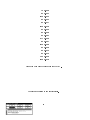
Figure 11 shows the structure of the le containing these data which will be the input for the
Workload Analyser Tool. The rst column represents the packet length, named length in the
format description in Fig. 14 (integer of four digits), and the second one is the interarrival time,
named delta in the format description in Fig. 14 (real of two and four digits before and after
the point, respectively). In what follows, we will present a few gures containing the operations
to be performed in order to specify the parameters of the analysis.
15
74 0.0009
60 0.0031
1345 0.0034
60 0.0033
60 0.0017
1345 0.0049
60 0.0005
60 0.0008
64 0.0021
577 0.0006
60 0.0027
1345 0.0068
64 0.0006
60 0.0010
60 0.0010
104 0.0049
1345 0.0018
Figure 11: Example of the input le for the WAT.
Figure 12: Denition of new specications.
16
Figure 13: Selection of the le type.
Figure 14: Specication of the format of the two variables within the input le.
17
Figure 15: Selection of the variables to be analyzed together with the transformations to be
applied and the trimming of the outliers.
Figure 16: Selection of control (percentile of outliers, random sample, number of clusters and
overall transformation), display and output specications.
18
Figure 17: Save of the specications.
Once the specications are saved into a le, it is possible to load them for editing (see Fig. 18).
19
Figure 18: Load of previously saved specications.
20
Once the specications have been dened, the user can perform the analysis by running the
Workload Analyser Tool with the Run option. The results obtained from the WAT after the
analysis of these specications with the data showed in Fig. 11 can be seen in the le which
name is specied in the item Output file of the Output specifications, i.e., data.out.
Figure 19: Run of the tool according to the pre-dened specications.
21
APPENDIX
A Use of the components of the interface
The interface is a set of basic components dened in the SDMF tool 5]. To facilitate the use of
this interface, we will briey review the various components.
A.1 Buttons
There are two dierent kinds of buttons within the interface:
1. action buttons
2. subform buttons
Both of them can be activated by simply clicking the left button of the mouse with the mouse
cursor located on the image of the button (i.e., the square surrounded label).
Figure 20: Examples of an action button (Define, Load or Run) and a subform button (Help).
A.2 Menus
There are dierent types of menu within the interface which can be invoked and used in the same
way. The following gures show a few examples of the menus provided within the interface.
22
Figure 21: Example of a window banner menu.
Figure 22: Example of a lename string item menu.
To open a menu (that is, to display all the items it consists of), the user needs to press the right
button of the mouse with the mouse cursor located on the image of the menu (i.e., the banner
of the window, the sum item or the lename string item).
To select an item, the user, with the mouse button pressed, needs to drag the mouse cursor to
locate it on the image of the item. When the mouse button is released, the item is selected and
the action associated to it executed.
Figure 23: Example of a sum item menu.
23
A.3 Sum items
Sum items are compositions of buttons and menus and can be used in either one or the other
\mode".
Using the \button mode", the user will change the value of the sum item, by selecting the value
of the sum item immediately after the current one. A few clicks will allow the user to scan
sequentially the list of values one by one.
Using the \menu mode", the user will display the list of values of the sum item and directly
select one.
Figure 24: Example of a sum item.
A.4 Integer range items
Integer range items are composed of two parts: an information part which displays the current
value of the integer range item and a slider which is used to change the value itself.
It is possible to move the slider to a specic position by clicking the left button of the mouse
with the mouse cursor located in the specied position within the slider rectangle. The user
can also make the cursor sliding by pressing the left button of the mouse with the mouse cursor
located on the black cursor of the slider and dragging the mouse to the left or to the right hand
side. While sliding the slider cursor, the changes of the values of the integer range item are
displayed. The value is set when the mouse button is released.
When the mouse cursor goes out of the slider rectangle, the slider cursor returns to its original
position.
24
Figure 25: Example of an integer range item.
A.5 String items
A string item is a eld containing either integer, real or textual values specied from the keyboard. Note that this denition does not apply to the lename string items, as we will specify
in the next section.
When the user wants to enter a value, he just needs to position the mouse cursor on the eld
he wants to edit and then he can type the value.
Each eld has a predened type associated to it. A test on the type is performed to avoid
possible errors (e.g., typing a character in an integer eld).
The DELETE key placed on the keyboard is the cancellation character.
Figure 26: Example of a string item.
A.6 Filename string items
Filename string items are a combination of string items and menus.
The user can directly insert the complete lename in the eld or he can use the right button of
the mouse to get the possible lename completions of what he has typed. This also gives the
possibility of selecting a lename from the list of the les available in the current directory. In
such a case, the lename eld is used as a menu with all the associated operations.
25
Figure 27: Example of a lename string item.
A.7 List items
List items are the building blocks of other types of item. This means that an element of a list
item can be a composition of any of the other types of item.
List items can be displayed in two dierent formats depending on the initial number of elements
in the list (see Figs. 28 and 29).
Figure 28: Example of a list item with no initial element.
Figure 29: Example of a list item with initial elements.
In the rst case (see Fig. 28), there are no initial elements in the list, the user only needs to
click on the extend list button to add a new element to the list.
In the second case (see Fig. 29), one or more elements already exist, by clicking on the \+"
button at the left hand side of any element of the list with the right button of the mouse a menu
is displayed (see Fig. 30). It is possible to:
insert a new element (just before the current one)
append a new element (just after the current one)
delete the current element of the list.
26
When the last element of the list is deleted, an empty list is obtained (see Fig. 28).
Figure 30: Example of the menu of a list item.
A.8 Resizing a window
In many cases, especially when list items are used, it is necessary to resize the window in order
to completely display its contents. This operation can be performed in various ways. The
standard windowing procedures are available. An alternative simple approach is to use the item
Fit contents in the banner menu of the window (submenu Resize, see Fig. 21), which will
automatically resize the window according to its contents.
27