Download DAME Suite α-release User's Guide - DAta Mining & Exploration

DAta Mining & Exploration
Program
DAME Suite
α-release
User’s Guide
DAME-MAN-NA-0007
Issue: 1.1
Date: June 28, 2010
Author: M. Brescia
Doc. : AlphaReleaseUserGuide_DAME-MAN-NA-0007-Rel1.1
1
Data Mining Suite Alpha Release User’s Guide
This document contains proprietary information of DAME project Board. All Rights Reserved.
DAta Mining & Exploration
Program
“Quelli che s'innamoran di pratica sanza scienza, son come 'l nocchiere,
ch'entra in navilio sanza timone o bussola, che mai ha certezza di dove si vada”
Leonardo Da Vinci
“No great pyramid was built in a day
nor shall be any great software without documentation”
Linus Torvald
“The future of Science is e-Science.
e-Science is where Information Technology meets scientists”
Jim Gray
“Artificial Intelligence is the exciting new effort to make computers
think . . . machines with minds, in the full and literal sense”
John Haugeland
“Always two there are… a master and an apprendist…
…the Force runs strong in your family!...”
Yoda, Jedi master
DAME Program
“we make science discovery happen”
2
Data Mining Suite Alpha Release User’s Guide
This document contains proprietary information of DAME project Board. All Rights Reserved.
DAta Mining & Exploration
Program
INDEX
1
2
3
Purpose ....................................................................................................................................................... 6
Introduction ................................................................................................................................................ 7
Machine Learning Theoretical Overview................................................................................................... 8
3.1 Supervised Machine Learning ............................................................................................................ 9
3.2 The functionality domains ................................................................................................................ 10
3.2.1
Classification ............................................................................................................................. 10
3.2.1.1
Confusion Matrix................................................................................................................ 11
3.2.1.2
K-fold Cross Validation ..................................................................................................... 12
3.2.2
Regression.................................................................................................................................. 13
3.3 The Machine Learning Models ......................................................................................................... 15
3.3.1
Multi Layer Perceptron .............................................................................................................. 15
3.3.1.1
Learning by Back Propagation ........................................................................................... 18
3.3.1.2
Generalization and statistics ............................................................................................... 20
3.3.1.2.1 Cross Entropy.................................................................................................................. 21
3.3.1.3
MLP Practical Rules ........................................................................................................... 23
3.3.1.3.1 Selection of neuron activation function .......................................................................... 24
3.3.1.3.2 Scaling input and target values ....................................................................................... 24
3.3.1.3.3 Number of hidden nodes ................................................................................................. 25
3.3.1.3.4 Number of hidden layers ................................................................................................. 25
3.3.1.3.5 Initializing Weights ......................................................................................................... 25
3.3.1.3.6 Momentum ...................................................................................................................... 25
3.3.1.3.7 Learning rate ................................................................................................................... 26
3.3.1.4
Implementation Details ...................................................................................................... 26
4 The Data Mining Suite User’s Manual..................................................................................................... 29
4.1 Overview ........................................................................................................................................... 30
4.2 User Registration and Access ........................................................................................................... 31
4.3 The command icons .......................................................................................................................... 32
4.4 Workspace Management ................................................................................................................... 33
4.5 Header Area ...................................................................................................................................... 37
4.6 Data Management ............................................................................................................................. 38
4.6.1
Upload user data ........................................................................................................................ 38
4.6.2
Create dataset files ..................................................................................................................... 40
4.6.2.1
Feature Selection ................................................................................................................ 41
4.6.2.2
Column Ordering ................................................................................................................ 42
4.6.2.3
Sort Rows by Column ........................................................................................................ 44
4.6.2.4
Column Shuffle .................................................................................................................. 45
4.6.2.5
Row Shuffle ........................................................................................................................ 46
4.6.2.6
Split by Rows ..................................................................................................................... 47
4.6.2.7
Dataset Scale ...................................................................................................................... 48
4.6.2.8
Single Column Scale ......................................................................................................... 49
4.6.3
Download data ........................................................................................................................... 51
4.6.4
Moving data files ....................................................................................................................... 51
4.7 Experiment Management .................................................................................................................. 52
4.7.1
Re-use of already trained networks ........................................................................................... 56
5 A practical example.................................................................................................................................. 60
5.1.1
The scientific problem: Photometric redshifts estimation ......................................................... 60
5.1.2
The Base of Knowledge (BoK) ................................................................................................. 61
5.1.3
Dataset Manipulation ................................................................................................................. 62
5.1.4
Experiment execution ................................................................................................................ 62
5.1.5
Experiment Results .................................................................................................................... 64
3
Data Mining Suite Alpha Release User’s Guide
This document contains proprietary information of DAME project Board. All Rights Reserved.
DAta Mining & Exploration
Program
TABLE INDEX
Tab. 1 – The DM models available in DAME alpha release ........................................................................... 30
Tab. 2 – Header Area Menu Options .............................................................................................................. 37
Tab. 3 – Abbreviations and acronyms ............................................................................................................. 68
Tab. 4 – Reference Documents ........................................................................................................................ 69
Tab. 5 – Applicable Documents....................................................................................................................... 70
FIGURE INDEX
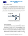
Fig. 1 – Where AI may fit into a knowledge process ......................................................................................... 8
Fig. 2 – A workflow based on supervised learning models ............................................................................... 9
Fig. 3 – An example of confusion matrix for a 3-class classification problem ............................................... 12
Fig. 4 – Some cases of K-fold cross validation ............................................................................................... 12
Fig. 5 – leave-one-out cross validation ........................................................................................................... 13
Fig. 6 – Example of a SLP to calculate the logic AND operation ................................................................... 17
Fig. 7 – A MLP able to calculate the logic XOR operation ............................................................................ 17
Fig. 8 – A MLP network trained by Back Propagation rule ........................................................................... 19
Fig. 9 – The sigmoid function and its first derivative ...................................................................................... 24
Fig. 10 – Typical Layered Application Architecture ....................................................................................... 29
Fig. 11 – Suite functional hierarchy ................................................................................................................ 30
Fig. 12 – The user login form to access at the web application ...................................................................... 32
Fig. 13 – The Web Application starting page (home) ..................................................................................... 32
Fig. 14 – The Web Application main commands ............................................................................................. 33
Fig. 15 – The right sequence to configure and execute an experiment workflow ........................................... 34
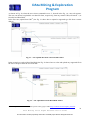
Fig. 16 – the button “New Workspace” at left corner of workspace manager window .................................. 34
Fig. 17 – the form field that appears after pressing the “New Workspace” button ........................................ 35
Fig. 18 – the active workspace created in the Workspace List Area ............................................................... 35
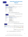
Fig. 19 – The GUI Header Area with all submenus open ............................................................................... 37
Fig. 20 – The Upload data feature open in a new tab ..................................................................................... 38
Fig. 21 – The Upload data from external URI feature .................................................................................... 39
Fig. 22 – The Upload data from Hard Disk feature ........................................................................................ 39
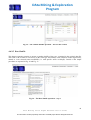
Fig. 23 – The Uploaded data (train.fits) in the Files Manager sub window ................................................... 40
Fig. 24 – The dataset editor tab with the list of available operations ............................................................. 41
Fig. 25 – The Feature Selection operation – step 1 ........................................................................................ 41
Fig. 26 – The Feature Selection operation – step 2 ........................................................................................ 42
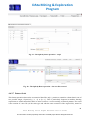
Fig. 27 – The Feature Selection operation – the new file created................................................................... 42
Fig. 28 – The Column Ordering operation – step 1 ........................................................................................ 43
Fig. 29 – The Column Ordering operation – step 2 ........................................................................................ 43
Fig. 30 – The Column Ordering operation – the new file created .................................................................. 43
Fig. 31 – The Sort Rows by Column operation – step 1 .................................................................................. 44
Fig. 32 – The Sort Rows by Column operation – step 2 .................................................................................. 44
Fig. 33 – The Sort Rows by Column operation – the new file created ............................................................ 45
Fig. 34 – The Column Shuffle operation – step 1 ............................................................................................ 45
Fig. 35 – The Column Shuffle operation – the new file created ...................................................................... 46
Fig. 36 – The Row Shuffle operation – step 1 ................................................................................................. 46
Fig. 37 – The Row Shuffle operation – the new file created............................................................................ 47
Fig. 38 – The Split by Rows operation – step 1 ............................................................................................... 47
Fig. 39 – The Split by Rows operation – step 2 ............................................................................................... 48
4
Data Mining Suite Alpha Release User’s Guide
This document contains proprietary information of DAME project Board. All Rights Reserved.
DAta Mining & Exploration
Program
Fig. 40 – The Split by Rows operation – the new files created ....................................................................... 48
Fig. 41 – The Dataset Scale operation – step 1............................................................................................... 49
Fig. 42 – The Dataset Scale operation – the new file created ......................................................................... 49
Fig. 43 – The Single Column Scale operation – step 1 ................................................................................... 50
Fig. 44 – The Single Column Scale operation – step 2 ................................................................................... 50
Fig. 45 – The Single Column Scale operation – the new file created.............................................................. 51
Fig. 46 – Creating a new experiment (by selecting icon “Experiment” in the workspace) ............................ 52
Fig. 47 – The new tab reporting the list of functionality-model couples available for experiments ............... 53
Fig. 48 – The use case selection for the experiment ........................................................................................ 53
Fig. 49 – The experiment parameter list for the use case “Full” in the regression case................................ 54
Fig. 50 – The experiment parameter list for the use case “Full” in the classification case ........................... 54
Fig. 51 – The experiment parameter list for the use case “Train” ................................................................. 55
Fig. 52 – The experiment parameter list for the use case “Test” ................................................................... 55
Fig. 53 – The experiment parameter list for the use case “Run”.................................................................... 56
Fig. 54 – Some different state of two concurrent experiments ........................................................................ 56
Fig. 55 – The operation to “move” an output file in the Workspace input file list ......................................... 57
Fig. 56 – The choice of input parameters of Run use case experiment ........................................................... 58
Fig. 57 – Some different state of two concurrent experiments ........................................................................ 59
Fig. 58 – The relation between redshift, color and source observed fluxes .................................................... 60
Fig. 59 – The 5 columns and first 13 rows of train.dat input file .................................................................... 61
Fig. 60 – The complete flow-chart of the experiment with MLP model .......................................................... 62
Fig. 61 – The selection of train.fits as Train Set ............................................................................................. 63
Fig. 62 – The selection of train.fits as Test Set and all fields compiled .......................................................... 63
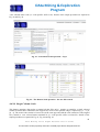
Fig. 63 – The myFirstExp output file list after the end of experiment ............................................................. 65
Fig. 64 – The contents of Full.log ................................................................................................................... 65
Fig. 65 – The contents of Full.tra (left) and Full.tes (right)............................................................................ 66
Fig. 66 – The contents of Full.csv ................................................................................................................... 66
Fig. 67 – The contents of Full.tes.jpeg ............................................................................................................ 66
Fig. 68 – The contents of Full.csv.jpeg............................................................................................................ 67
Fig. 69 – Best Trend of zspec versus zphot redshifts for the Main Galaxy sample ......................................... 67
5
Data Mining Suite Alpha Release User’s Guide
This document contains proprietary information of DAME project Board. All Rights Reserved.
DAta Mining & Exploration
Program
1 Purpose
he present document has been extracted from the DAME Book1, a big document containing all
scientific and technological information behind the strategy of DAME, including design, development
and implementation issues, together with instruction on how to use and maintain the entire
infrastructure.
T
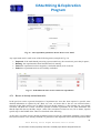
This document is the reference manual of the official alpha release of the data mining Suite. The alpha is
available for test at the following address: http://143.225.93.239:8080/MyDameFE/
So far it has the basic role to support testing users (the victims…!) to use the software toolset in the right and
more satisfying way.
The available features, in terms of data mining models and functional use cases for scientific experiments,
are voluntarily limited within the alpha release, although sufficient to verify the internal mechanisms and
user-machine interaction modes at the base of the DM Suite and of its next releases.
As the reader probably already knows, the data mining models provided in DAME are derived from the
machine learning and Artificial Intelligence paradigms. Some of the end users in principle could not be
familiar with such models. So far, a theoretical quick and practice-oriented overview of such techniques is
required.
The document is hence organized as follows:
•
•
•
•
•
1
Chapter 2 is a simple Introduction to DAME Program “proposition value”;
Chapter 3 introduces the reader through theoretical and algorithmic aspects concerning machine
learning models and functional domains currently available in the released software;
Chapter 4 is the user’s reference and guide to use the DM Suite current release;
Chapter 5 reports a practical example of scientific use case solved by the DM Suite current release;
Last pages host tables with “Abbreviations & Acronyms”, “Reference” and “Applicable” document
lists and the acknowledgments. All over the document the references are labeled as [Rxx] for
“Reference” documents and [Axx] for “Applicable” documents (xx is the incremental index as
reported in the list tables). “Applicable” documents are not public references (technical documents
internal to the DAME working group) included for quick technical references. Users external to the
working group may ask to consult (privately) these documents by e-mail, motivating the reasons.
The complete list of the internal documentation is available at the following address of the program
official website: http://voneural.na.infn.it/DAME_DOCUMENTATION_LIST.html
Currently under preparation.
6
Data Mining Suite Alpha Release User’s Guide
This document contains proprietary information of DAME project Board. All Rights Reserved.
DAta Mining & Exploration
Program
2 Introduction
D
AME arises as a single project at the beginning of 2007. The original name was VO-Neural, derived
from earlier Astroneural project, whose main goal was to create a software framework to solve
specific astrophysical problems by employing experienced methodologies coming from Machine
Learning and Artificial Intelligence paradigms and architectures. After first two years of design activity, VONeural definitely changes into DAME.
Since the beginning of the project, its members observed the following facts.
The explosion of technology progress in digital processing, computer Science, high performance and
distributed computing, astronomical telescopes and focal plane instrumentation, imposed a new approach to
make Science, able to explore in an efficient way the incoming “tsunami” of petabytes of data collected in
worldwide distributed archives and data centres: the new frontier became the e-Science.
Indeed, this trend has rapidly issued the fourth paradigm of Science, recently recognized at a planetary level,
after theory, experimentation and simulations: data mining, or equivalently, Knowledge Discovery in
Databases (KDD), [R6].
These considerations convinced our group to pursue their scientific goals from a new, more organized,
coherent and efficient perspective. So far, the idea was to create a program, as a whole infrastructure capable
to merge in an homogeneous way scientific products with the state of the art of technology and astrophysics
trends, where the multi-disciplinary experience and the data mining research would be the engine of the
common goal. Moreover, the immediate consequence was the awareness that such an infrastructure could
represent a standard gateway to accomplish the fourth paradigm for further discoveries in the e-Science, in
particular e-Astrophysics, [A1]. In other words, a product to be shared with the entire scientific community
in an “open and easy way”.
Open means basically easily extendable in terms of functionalities and data mining models able to be
employed in the general astrophysics research and data exploration at large.
While the term easy is referred to the features offered to the community users, in terms of high computing
power and user-friendly scientific applications available “at one click”, through a simple web browser.
In other words, this product inherits advanced technological aspects made available to users in an absolutely
transparent way, leaving them to focus their brain energies to organize and execute scientific experiments
and workflows2.
The only effort required to the end user is to have a bit of faith in Artificial Intelligence and a little amount of
patience to learn basic principles of its models and strategies.
By merging for fun two famous commercial taglines we say: “Think different, Just do it!”
(casually this is an example of text mining...!)
2
Workflow is hereinafter synonymous of pipeline.
7
Data Mining Suite Alpha Release User’s Guide
This document contains proprietary information of DAME project Board. All Rights Reserved.
DAta Mining & Exploration
Program
3 Machine Learning Theoretical Overview
O
ne of main breakthroughs in modern Astrophysics is the reached physical limit of observations
(single photon counting) at almost all wavelengths, with giant and by now linear detectors. So far,
like all scientific disciplines focusing their discoveries on collected data exploration, there is a strong
need to employ e-science
science methodology and
and tools in order to gain new insights on the Universe. But this
mainly depend on the capability to recognize patterns or trends in the parameter space (i.e. physical laws),
possibly by overcoming the human limit of 3D brain vision, and
and to use known patterns (coming from
observations and simulations as well) as BoK (Base of Knowledge) to infer knowledge on self-adaptive
self
models in order to make them able to generalize feature correlations and to gain new discoveries (for
example outliers identification) through the unbiased exploration of new collected data. These requirements
are perfectly matching the paradigm of machine learning techniques based on the Artificial Intelligence
postulate, [R7].
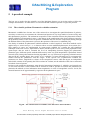
Fig. 1 – Where AI may fit into a knowledge process
Hence, as shown in Fig. 1, at all steps of a scientific pipeline process,
process machine learning rules can be applied,
applied
[R8].. Let us better know this methodology. It exists a basic dichotomy in Machine Learning,
Learning [R2, R3], by
distinguish between supervised
sed and unsupervised methodologies,
methodologies, as described in the following.
The Greek philosopher Aristotle was one of the first to attempt to codify "right thinking," that syllogism is,
irrefutable reasoning processes. His syllogisms provided patterns for argument structures that always yielded
correct conclusions
ons when given correct premises; for example, "Socrates is a man; all men are mortal;
therefore, Socrates is mortal." These laws of thought were logic supposed to govern the operation
oper
of the
mind; their study initiated the field called “logic”.
Logicians in the 19th century developed a precise notation for statements about all kinds of things in the
world and about the relations among them3.
By 1965, programs existed that could, in principle, solve any solvable problem described in logicist logical
notation. The so-called logicist tradition within Artificial Intelligence
ntelligence hopes to build on such programs to
create intelligent systems and the Machine Learning theory represents their demonstration discipline. A
reinforcement in this direction came out by integrating Machine Learning paradigm with statistical principles
following the Darwin’s Nature evolution laws,
law [R1, R11].
3
Contrast this with ordinary arithmetic notation, which provides mainly for equality and inequality statements about
numbers.
8
Data Mining Suite Alpha Release User’s Guide
This document contains proprietary information of DAME project Board. All Rights Reserved.
DAta Mining & Exploration
Program
3.1 Supervised Machine Learning
In supervised machine learning we have a set of data points or observations for which we know the desired
output, class, target variable or outcome.
outcome. The outcome may take one of many values called classes or labels.
A classic example is that given a few thousand emails for which we know whether they are spam or ham
(their labels), the idea is to create a model that is able to deduce whether new, unseen
unse n emails are spam or not.
In other words, we are creating a mapping function where the inputs are the email's sender, subject, date,
time, body,
ody, attachments and other attributes, and the output is a prediction as to whether the email is spam or
ham. The target variable is in fact providing some level of supervision in that it is used by the learning
algorithm to adjust parameters or make decisions
decisions that will allow it to predict labels for new data. Finally of
note, when the algorithm is predicting labels of observations we call it a classifier.. Some classifiers are also
capable of providing a probability of a data point belonging to class in which
which case it is often referred to a
probabilistic model or a regression - not to be confused with a statistical regression model.
model
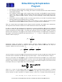
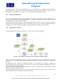
A common workflow approach for supervised learning analysis is shown in the diagram below (Fig.
(
2).
Fig. 2 – A workflow based on supervised learning models
The process is:
1. Scale and prepare training data: First we build input vectors that are appropriate for feeding into
our supervised learning algorithm.
2. Create a training set and a validation set by randomly splitting the universe of data. The training
set is the data that the classifier uses to learn how to classify the data, whereas the validation
vali
set is
used to feed the already trained model in order to get an error rate (or other measures and techniques)
that can help us identify the classifier's performance and accuracy. Typically you will use more
training data (maybe 80% of the entire universe)
universe) than validation data. Note that there is also crossvalidation), but that is beyond the scope of this article.
3. Train the model. We take the training data and we feed it into the algorithm. The end result is a
model that has learned (hopefully) how to predict our outcome given new unknown data.
4. Validation and tuning: After we've created a model, we want to test its accuracy. It is critical to do
this on data that the model has not seen yet - otherwise you are cheating. This is why on step 2 we
separated
ted out a subset of the data that was not used for training. We are indeed testing our model's
generalization capabilities. It is very easy to learn every single combination of input vectors and their
mappings to the output as observed on the training data,
data, and we can achieve a very low error in
9
Data Mining Suite Alpha Release User’s Guide
This document contains proprietary information of DAME project Board. All Rights Reserved.
DAta Mining & Exploration
Program
doing that, but how does the very same rules or mappings perform on new data that may have
different input to output mappings? If the classification error of the validation set is very big
compared to the training set's, then we have to go back and adjust model parameters. The model will
have essentially memorized the answers seen in the training data, losing its generalization
capabilities. This is called over fitting, and there are various techniques for overcoming it.
5. Validate the model's performance. There are numerous techniques. The model's accuracy can be
improved by changing its structure or the underlying training data. If the model's performance is not
satisfactory, change model parameters, inputs and or scaling, go to step 3 and try again.
6. Use the model to classify new data. In production. Profit!
3.2 The functionality domains
In the data mining scenario, the machine learning model choice should always be accompanied by the
functionality domain. To be more precise, some machine learning models can be used in a same functionality
domain, because it represents the functional context in which it is performed the exploration of data.
Examples of such domains are:
•
•
•
•
•
•
•
•
Dimensional reduction;
Classification;
Regression;
Clustering;
Segmentation;
Statistical data analysis;
Forecasting;
Data Mining Model Filtering;
In the following we focus the attention on Classification and Regression only, being the two functional
domains available in the current alpha release of the data mining application Suite.
3.2.1
Classification
Statistical classification is a procedure in which individual items are placed into groups based on quantitative
information on one or more features inherent to the items (referred to as features) and based on a training set
of previously labelled items.
A classifier is a system that performs a mapping from a feature space X to a set of labels Y. Basically a
classifier assigns a pre-defined class label to a sample.
Formally, the problem can be stated as follows: given training data {(x_1,y_1),...,(x_n, y_n)} (where x_i are
vectors) a classifier h:X->Y maps an object x ε X to its classification label y ε Y.
Different classification problems could arise:
a) crispy classification: given an input pattern x (vector) the classifier returns its computed label y (scalar).
b) probabilistic classification: given an input pattern x (vector) the classifier returns a vector y which
contains the probability of y_i to be the "right" label for x. In other words in this case we seek, for each input
vector, the probability of its membership to the class y_i (for each y_i).
10
Data Mining Suite Alpha Release User’s Guide
This document contains proprietary information of DAME project Board. All Rights Reserved.
DAta Mining & Exploration
Program
Both cases may be applied to both "two-class" and "multi-class" classification. So the classification task
involves, at least, three steps:
•
•
•
training, by means of a training set (INPUT: patterns and target vectors, or labels; OUTPUT: an
evaluation system of some sort);
testing, by means of a test set (INPUT: patterns and target vectors, requiring a valid evaluation
system from point 1; OUTPUT: some statistics about the test, confusion matrix, overall error, bitfail
error, as well as the evaluated labels);
evaluation, by means of an unlabelled dataset (INPUT: patterns, requiring a valid evaluation
systems; OUTPUT: the labels evaluated for each input pattern);
Because of the supervised nature of the classification task, the system performance can be measured by
means of a test set during the testing procedure, in which unseen data are given to the system to be labelled.
The overall error somehow integrates information about the classification goodness. However, when a data
set is unbalanced (when the number of samples in different classes varies greatly) the error rate of a classifier
is not representative of the true performance of the classifier. A confusion matrix can be calculated to easily
visualize the classification performance: each column of the matrix represents the instances in a predicted
class, while each row represents the instances in an actual class. One benefit of a confusion matrix is the
simple way to see if the system is mixing two classes.
Optionally (some classification methods does not require it by its nature or simply as a user choice), one
could need a validation procedure.
Validation is the process of checking if the classifier meets some criterion of generality when dealing with
unseen data. It can be used to avoid over-fitting or to stop the training on the base of an "objective" criterion.
With “objective” we intend a criterion which is not based on the same data we have used for the training
procedure. If the system does not meet this criterion it can be changed and then validated again, until the
criterion is matched or a certain condition is reached (for example, the maximum number of epochs). There
are different validation procedures. One can use an entire dataset for validation purposes (thus called
validation set); this dataset can be prepared by the user directly or in an automatic fashion.
In some cases (e.g. when the training set is limited) one could want to apply a "cross validation" procedure,
which means partitioning a sample of data into subsets such that the analysis is initially performed on a
single subset, while the other subset(s) are retained for subsequent use in confirming and validating the initial
analysis.
Different types of cross validation may be implemented, e.g. k-fold, leave-one-out, etc.
Summarizing we can safely state that a common classification training task involves:
•
•
•
the training set to compute the model;
the validation set to choose the best parameters of this model (in case there are "additional"
parameters that cannot be computed based on training);
the test data as the final "judge", to get an estimate of the quality on new data that are used neither to
train the model, nor to determine its underlying parameters or structure or complexity of this model;
The validation set may be provided by the user, extracted from the software or generated dynamically in a
cross validation procedure. In the following we underline some practical aspects connected with the
validation techniques, as implemented in our classification models.
3.2.1.1 Confusion Matrix
This is a simple diagnostic instrument useful to estimate the efficiency of the classification model (such as a
supervised neural network). It basically consists in a matrix with the values of target vector and the output
values produced from the model, respectively, on its rows and columns, [A12]. In addition it allows to
11
Data Mining Suite Alpha Release User’s Guide
This document contains proprietary information of DAME project Board. All Rights Reserved.
DAta Mining & Exploration
Program
calculate the success rate, e.g. the percentage of objects correctly classified from the model. The number of
"bit fault" that the model badly classifies and the percentage of correctly classified objects for each class.
In the matrix the element corresponding to row i and column j is the absolute number
numb or case percentage of
“true” class i classified in the class j. On the main diagonal the correct classified cases are reported. The
others are classification errors.
3
classification
ication problem
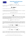
Fig. 3 – An example of confusion matrix for a 3-class
In the example of Fig. 3 we have a 3-class
3 class classification problem results. The original training set consists of
200 patterns.
In the class A there are 87 cases: 60 correctly classified as A; 27 wrongly classified, of which 14 as B and 13
as C.
So far, for the class A the accuracy is 60 / 87 = 69,0%. For the class B the accuracy is 34 / 60 = 56,7% and
for class C 42 / 53 = 79,2%.
c
are
The whole accuracy is hence: (60 + 34 + 42) / 200 = 136 / 200 = 68,0%. The errors (bad classification)
then 32%, e.g. 64 cases on 200 patterns.
patterns
The classification result depends not only on the percentages, but also on the relevance of single kinds of
errors. In the example, if class C is the most important to be classified, the final result of the classification
can be considered successful.
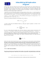
3.2.1.2 K-fold
fold Cross Validation
The cross validation is a statistical method useful to validate a predictive classification model. Having a data
sample this is divided into subsets, some of them used for the training phase (training set),
set) while the others
employed to compare the model prediction capability (validation set). By varying the value of K (different
splitting of the data sets) it is possible to evaluate the prediction accuracy of the trained model, Fig. 4.
Fig. 4 – Some cases of K-fold cross validation
The K-fold cross-validation divides the whole dataset into K subsets, each of them is alternately excluded
from the validation set.
12
Data Mining Suite Alpha Release User’s Guide
This document contains proprietary information of DAME project Board. All Rights Reserved.
DAta Mining & Exploration
Program
There is also a special
ial case, named leave-one-out
l
cross validation, where alternately only one pattern is
excluded at each validation run, Fig. 5.
Fig. 5 – leave-one-out cross validation
In practice all data are used for the training and test phases in an independent way. In this case we obtain K
classifiers (2 ≤ K ≤ n) whose outputs can be used to obtain a mean evaluation. The downside of this method
is that it could result very expensive in terms of computing time in case of massive datasets.
3.2.2
Regression
Regression methods bring out relations between variables, especially whose relation is imperfect (i.e it has
not one y for each given x). Just as an example, the relation in a DM design team between brain weight and
working capability of the members is a typical “imperfect relationship” (any reference is purely casual…).
The term regression is historically coming from biology in genetic transmission through generations, where
for example it is known that tall fathers have tall sons, but not as tall on the average as the fathers. The trend
to transmit on average genetic features, but not exactly in the same quantity, was what the scientist Galton
defined as regression,, more exactly regression toward the mean.
This is the first item I founded through a short immersion on the argument.
But what is regression?
on? Strictly speaking it is very difficult to find a precise definition. We prefer to deal
with two meanings for regression, that can be addressed as data table statistical correlation (usually column
averages) and as fitting of a function.
function
About the firstt meaning, let start with a very generic example: suppose to have two variables x and y, where
for each small interval of x there is a distribution of corresponding y. We can always compute a summary of
the y values for that interval. The summary might be for example the mean, median or even the geometric
mean. Let fix the points , ),
the average y for that interval.
), where is the center of the ith interval and Then the fixed points will fall close to a curve that could summarize them, possibly
possibly close to a straight line.
Such a smooth curve approximates the regression curve called the regression of y on x.
x By generalizing the
example, the typical application is when the user has a table (let say a series of input patterns coming from
any experience
erience or observation) with some correspondences between intervals of x (table raws) and some
distributions of y (table columns), representing a generic correlation not well known (i.e. imperfect as
introduced above) between them. Once we have such a table,
table, we want for example to clarify or accent the
relation between the specific values of one variable and the corresponding values of the other. If we want an
average, we might compute the mean or median for each column. Then to get a regression, we might plot
p
these averages against the midpoints of the class intervals.
Given the example in mind let’s try to extrapolate the formal definition of regression (in its first meaning).
In a mathematical sense, when for each value of x there is a distribution of y, with density f(y|x) and the
mean4 value of y for that x given by
y ( x) =
+∞
∫ yf ( y | x)dy
−∞
4
Here the use of the mean as statistical operator
operator is only an example. It can be replaced by the median or other more
complex methods.
13
Data Mining Suite Alpha Release User’s Guide
This document contains proprietary information of DAME project Board. All Rights Reserved.
DAta Mining & Exploration
Program
then the function defined by the set of ordered pairs ( ( x, y ( x )) is called the regression of y on x. Depending
on the statistical operator used, the resulting regression line or curve on the same data can present a slightly
different slope.
In the practical astrophysical cases, we usually do not have continuous populations with known functional
forms. But the data may be very extensive. In these cases it is possible to break one of the variables into
small intervals and compute averages for each of them. Then, without severe assumptions about the shape of
the curve, essentially get a regression curve. What the regression curve does is essentially to give a, let say,
“big summary” for the averages for the distributions corresponding to the set of x’s. One can go further and
compute several different regression curves corresponding to the various percentage points of the
distributions and thus get a more complete picture of the input data set. Of course often it is an incomplete
picture for a set of distributions! But in this first meaning of regression, when the data are more sparse, we
may find that sampling variation makes impractical to get a reliable regression curve in the simple averaging
way described. From this assumption, it descends the second meaning of regression.
Usually it is possible to introduce a smoothing procedure, applying it either to the column summaries or to
the original values of y’s (of course after an ordering of y values in terms of increasing x). In other words we
assume a shape for the curve describing the data, for example linear, quadratic, logarithmic or whatever.
Then we fit the curve by some statistical method, often least-squares. In practice, we do not pretend that the
resulting curve has the perfect shape of the regression curve that would arise if we had unlimited data, but
simply we obtain an approximation. In other words we intend the regression of data in terms of forced fitting
of a functional form. The real data present intrinsic conditions that make this second meaning as the official
regression use case, instead of the first, i.e. curve connecting averages of column distributions. We ordinarily
choose for the curve a form with relatively few parameters and then we have to choose the method to fit it. In
many manuals sometimes it might be founded a definition probably not formally perfect, but very clear: by
regressing one y variable against one x variable means to find a carrier for x.
This introduce possible more complicated scenarios in which more than one carrier of data can be founded.
In these cases it has the advantage that the geometry can be kept to three dimensions (with two carriers) up to
n-dimensional spaces (n>3, with more than two carriers regressing input data). Clearly, both choosing the set
of carriers from which a final subset is to be drawn and choosing that subset can be most disconcerting
processes.
In substance we can declare a simple, important use of regression, consisting in:
To get a summary of data, i.e. to locate a representative functional operator of the data set, in a statistical
sense (first meaning) or via an approximated trend curve estimation (second meaning).
And a more common use of regression:
•
•
•
For evaluation of unknown features hidden into the data set;
For prediction, as when we use information from several weather or astronomical seeing stations to
predict the probability of rain or the turbulence growing in the atmosphere;
For exclusion. Usually we may know that x affects y, and one could be curious to know whether z
affects5 y too. In this case one approach would take the effects of x out of y and see if what remains
is associated with z. In practice this can be done by an iterative fitting procedure by evaluating at
each step the residual of previous fitting.
This is not exhaustive of the regression argument, but simple considerations to help the understanding of the
regression term and the possibility to extract basic specifications for the use case characterization in the
design phase.
5
Here “affects” is a shorthand for “is associated with, possibly, but not certainly, through a causal mechanism”.
14
Data Mining Suite Alpha Release User’s Guide
This document contains proprietary information of DAME project Board. All Rights Reserved.
DAta Mining & Exploration
Program
3.3 The Machine Learning Models
This paragraph is intended to furnish a theoretical overview of some machine learning models to be
associated with single or multiple functionality domains, in order to be used to perform practical scientific
experiments with such techniques. Only models foreseen to be implemented in the DAME infrastructure will
be treated.
3.3.1
Multi Layer Perceptron
The MLP architecture is one of the most typical feed-forward neural network model, [R9]. The term feedforward is used to identify basic behavior of such neural models, in which the impulse is propagated always
in the same direction, e.g. from neuron input layer towards output layer, through one or more hidden layers
(the network brain), by combining weighted sum of weights associated to all neurons (except the input
layer).
As easy to understand, the neurons are organized in layers, with proper own role. The input signal, simply
propagated throughout the neurons of the input layer, is used to stimulate next hidden and output neuron
layers. The output of each neuron is obtained by means of an activation function, applied to the weighted
sum of its inputs. Different shape of this activation function can be applied, from the simplest linear one up
to sigmoid, arctan or tanh (or a customized function ad hoc for the specific application). The number of
hidden layers represents the degree of the complexity achieved for the energy solution space in which the
network output moves looking for the best solution. As an example, in a typical classification problem, the
number of hidden layers indicates the number of hyper-planes used to split the parameter space (i.e. number
of possible classes) in order to classify each input pattern.
There is a special type of activation function, called softmax, [A13].
As known the activation function can be either linear or non-linear, depending on whether the network must
learn a regression problem or should perform a classification.
Activation functions, for the hidden units, introduce the non linearity into the network. Without non linearity,
the hidden units would not render the NN more powerful than just the perceptrons with only input and output
units (the linear function of linear functions is again a linear function). In other words, it is the non linearity
(i.e., the capability to represent non linear functions) that makes multilayer networks so powerful.
For the hidden units, sigmoid activation functions (for binary problems), see equation (2), or softmax (for
multi class problem), are usually better to use instead of the threshold activation functions, see equation (1).
0 if a < 0
f ( x) = 
1 else
1
f ( x) =
1 + e− a
(1)
(2)
Networks with threshold units are difficult to train, because the error function is stepwise constant, hence the
gradient either does not exist or is zero, thus making it impossible to use back propagation (a powerful and
computationally efficient algorithm for finding the derivatives of an error function with respect to the
weights and biases in the network) or the more efficient gradient-based training methods.
With sigmoid units, a small change in the weights will usually produce a large change in the outputs, which
makes it possible to tell whether that change in the weights is good or useless. With threshold units, a small
change in the weights will often produce no change in the outputs. For the output units, activation functions
suited to the distribution of the target values are:
15
Data Mining Suite Alpha Release User’s Guide
This document contains proprietary information of DAME project Board. All Rights Reserved.
DAta Mining & Exploration
Program
•
•
•
•
•
For binary (0/1) targets, the logistic sigmoid function is an excellent choice;
choice
For categorical targets using 1-of-C
1 C coding, the softmax activation function is the natural extension
ext
of the logistic function;
For continuous-valued
valued targets with a bounded range, the logistic and hyperbolic tangent functions
can be used, where you either scale the outputs to the range of the targets or scale the targets to the
range of the output activation function ("scaling" means multiplying by and
an adding appropriate
constants);
If the target values are positive but have no known upper bound, you can use an exponential output
activation function, but you must beware of overflow;
For continuous-valued
valued targets with no bounds, use the identity or "linear" activation function (which
amounts to no activation function) unless you have a very good reason to do otherwise.
There are certain
ertain natural associations between output activation functions and various noise distributions.
The output activation function is the inverse of what statisticians call the "link function".
In order to ensure that the outputs can be interpreted as posterior
posterior probabilities, they must be comprised
between zero and one, and their sum must be equal to one. This constraint also ensures that the distribution is
correctly normalized. In practice this is, for multi-class
multi class problems, achieved by using a softmax activation
activa
function in the output layer. The purpose of the softmax activation function is to enforce these constraints on
the outputs. Let the network input to each output unit be qi, i = 1,...,c, where c is the number of categories.
Then the softmax output pi is:
pi =
eqi
c
∑e
qj
j =1
Statisticians usually call softmax a "multiple logistic" function. Softmax equation is also known as
normalized exponential function. It reduces to the simple logistic function when there are only two
categories. Suppose you choose to set q2 = 0:
p1 =
e q1
c
∑e
qj
e q1
1
= q1 0 =
e − e 1 + e − q1
j =1
The term softmax is used because this activation function represents a smooth version of the winner-takes-all
winner
activation model in which the unit with the largest input has output +1 while all other units have output 0.
The base of the MLP is the Perceptron,
Perceptron a type of artificial neural network invented in 1957 at the Cornell
Aeronautical Laboratory by Frank Rosenblatt. It can be seen as the simplest kind of feedforward neural
network: a linear classifier. The Perceptron is a binary classifier which maps its input x (a real-valued vector)
to an output value f(x) (a single binary value) across the matrix.
where w is a vector of real-valued
valued weights and
is the dot product (which computes a weighted
sum). b is the 'bias', a constant term that does not depend on any input value. The value of f(x) (0 or 1) is
used to classify x as either a positive or a negative instance, in the case of a binary classification problem.
16
Data Mining Suite Alpha Release User’s Guide
This document contains proprietary information of DAME project Board. All Rights Reserved.
DAta Mining & Exploration
Program
If b is negative, then the weighted combination
combination of inputs must produce a positive value greater than | b | in
order to push the classifier neuron over the 0 threshold. Spatially, the bias alters the position (though not the
orientation) of the decision boundary. The Perceptron learning algorithm does not terminate if the learning
set is not linearly separable. The Perceptron is considered the simplest kind of feed-forward
forward neural network.
The earliest kind of neural network is a Single Layer Perceptron (SLP) network, which consists of a single
layer of output nodes; the inputs are fed directly to the outputs via a series of weights. In this way it can be
considered the simplest kind of feed-forward
feed forward network. The sum of the products of the weights and the inputs
is calculated in each node, and if the value is above some threshold (typically 0) the neuron fires and takes
the activated value (typically 1); otherwise it takes the deactivated value (typically -1).
1).
Fig. 6 – Example of a SLP to calculate the logic AND operation
Neurons with this kind of activation function are also called artificial neurons or linear threshold units,
units as
described by Warren McCulloch and Walter Pitts in the 1940s.
A Perceptron can be created using any values for the activated and deactivated states as long as the threshold
value lies between the two. Most perceptrons have outputs of 1 or -11 with a threshold of 0 and there is some
evidence that such networks can be trained more quickly than networks created from nodes with different
activation and deactivation values. SLPs are only capable of learning linearly separable patterns. In 1969 in a
famous monograph entitled Perceptrons Marvin Minsky and Seymour Papert showed that it was
wa impossible
for a single-layer Perceptron network to learn an XOR function.
Although a single threshold unit is quite limited in its computational power, it has been shown that networks
of parallel threshold units can approximate any continuous function from
from a compact interval of the real
numbers into the interval [-1,1].
1,1]. So far, it was introduced the model Multi Layer Perceptron.
Fig. 7 – A MLP able to calculate the logic XOR operation
This class of networks consists of multiple layers of computational units, usually interconnected in a feedfeed
forward way. Each neuron in one layer has directed connections to the neurons of the subsequent layer. In
many applications the units of these networks apply a continuous activation function.
17
Data Mining Suite Alpha Release User’s Guide
This document contains proprietary information of DAME project Board. All Rights Reserved.
DAta Mining & Exploration
Program
The universal approximation theorem [R12] for neural networks states that every continuous function that
maps intervals of real numbers to some output interval of real numbers can be approximated arbitrarily
closely by a multi-layer Perceptron with just one hidden layer. This result holds only for restricted classes of
activation functions, e.g. for the sigmoidal functions.
An extension of the universal approximation theorem states that the two layers architecture is capable of
universal approximation and a considerable number of papers have appeared in the literature discussing this
property. An important corollary of these results is that, in the context of a classification problem, networks
with sigmoidal non-linearity and two layer of weights can approximate any decision boundary to arbitrary
accuracy. Thus, such networks also provide universal non-linear discriminate functions. More generally, the
capability of such networks to approximate general smooth functions allows them to model posterior
probabilities of class membership. Since two layers of weights suffice to implement any arbitrary function,
one would need special problem conditions, or requirements to recommend the use of more than two layers.
Furthermore, it is found empirically that networks with multiple hidden layers are more prone to getting
caught in undesirable local minima.
Astronomical data do not seem to require such level of complexity and therefore it is enough to use just a
double weights layer, i.e. a single hidden layer.
The MLP consists of three or more layers (an input and an output layer with one or more hidden layers) of
nonlinearly-activating nodes. Each node in one layer connects with a certain weight wij to every node in the
following layer.
What is different in such a neural network architecture is typically the learning algorithm used to train the
network. It exists a dichotomy between supervised and unsupervised learning methods.
As in all supervised models, the network must be firstly trained (training phase), in which the input patterns
are submitted to the network as couples (input, desired known output). The feed-forward algorithm is then
achieved and at the end of the input submission, the network output is compared with the corresponding
desired output in order to quantify the learning quote. It is possible to perform the comparison in a batch way
(after an entire input pattern set submission) or incremental (the comparison is done after each input pattern
submission) and also the metric used for the distance measure between desired and obtained outputs, can be
chosen accordingly problem specific requirements (usually the Euclidean distance is used).
After each comparison and until a desired error distance is unreached (typically the error tolerance is a precalculated value or a constant imposed by the user), the weights of hidden layers must be changed
accordingly to a particular law or learning technique.
After the training phase is finished (or arbitrarily stopped), the network should be able not only to recognize
correct output for each input already used as training set, but also to achieve a certain degree of
generalization, i.e. to give correct output for those inputs never used before to train it. The degree of
generalization varies, as obvious, depending on how “good” has been the learning phase. This important
feature is realized because the network doesn’t associates a single input to the output, but it discovers the
relationship present behind their association. After training, such a neural network can be seen as a black box
able to perform a particular function (input-output correlation) whose analytical shape is a priori not known.
In order to gain the best training, it must be as much homogeneous as possible and able to describe a great
variety of samples. Bigger the training set, higher will be the network generalization capability.
Despite of these considerations, it should always taken into account that neural networks application field
should be usually referred to problems where it is needed high flexibility (quantitative result) more than high
precision (qualitative results).
3.3.1.1 Learning by Back Propagation
Multi-layer networks use a variety of learning techniques, the most popular being back-propagation (BP).
Here, the output values are compared with the correct answer to compute the value of some predefined errorfunction. By various techniques, the error is then fed back through the network. Using this information, the
algorithm adjusts the weights of each connection in order to reduce the value of the error function by some
small amount. After repeating this process for a sufficiently large number of training cycles, the network will
18
Data Mining Suite Alpha Release User’s Guide
This document contains proprietary information of DAME project Board. All Rights Reserved.
DAta Mining & Exploration
Program
usually converge to some state where the error of the calculations is small. In this case,
ca one would say that
the network has learned a certain target function. To adjust weights properly, one applies a general method
for non-linear optimization that is called gradient descent. For this, the derivative of the error function with
respect to the
he network weights is calculated, and the weights are then changed such that the error decreases
(thus going downhill on the surface of the error function). For this reason, back-propagation
back propagation can only be
applied on networks with differentiable activation functions.
fu
In general, the problem of teaching a network to perform well, even on samples that were not used as
training samples, is a quite subtle issue that requires additional techniques. This is especially important for
cases where only very limited numbers of training samples are available. The danger is that the
network overfits the training data and fails to capture the true statistical process generating the
data. Computational learning theory is concerned with training classifiers on a limited amount
am
of data. In the
context of neural networks a simple heuristic, called early stopping, often ensures that the network will
generalize well to examples not in the training set.
Other typical problems of the back-propagation
propagation algorithm are the speed of convergence and the possibility of
ending up in a local minimum of the error function. Today there are practical solutions that make backback
propagation in multi-layer
layer perceptrons the solution of choice for many machine learning tasks.
Fig. 8 – A MLP network trained by Back Propagation rule
It is a supervised learning method, and it is an implementation of the Delta rule, Fig. 8, where as an example
it is supposed to use sigmoidal activation function for all neurons of all layers.
layers. It requires a teacher that
knows, or can calculate, the desired output for any given input. It is most useful for feed-forward networks
(networks that have no feedback,
ck, or simply, that have no connections that loop). The term is an abbreviation
for "backwards propagation of errors". Back Propagation requires that the activation function used by
the artificial neurons (or "nodes") is differentiable. Main formulas are:
19
Data Mining Suite Alpha Release User’s Guide
This document contains proprietary information of DAME project Board. All Rights Reserved.
DAta Mining & Exploration
Program
_
= _ + + Δ_
_
= _ + ℎ + Δ_
(7)
(8)
Where:
•
•
•
•
(3) and (4) are the activation function for a generic neuron of the, respectively, hidden layer and
output layer. This is the mechanism to process and flow the input pattern signal through the
“forward” or bottom-up phase (from input neuron layer up to output neuron layer);
At the end of the “forward” phase the network error is calculated (inner argument of the (5)), to be
used during the “backward” or top-down phase to modify (adjust) neuron weights;
(5) and (6) are the descent gradient calculations of the “backward” phase, respectively, for a generic
neuron of the output and hidden layer;
(7) and (8) are the most important laws of the backward phase. They represent the weight
modification laws, respectively, between output and hidden layers (7) and between hidden-input (or
hidden-hidden if more than one hidden layer is present in the network topology) layers. The new
weights are adjusted by adding to the old ones two terms:
o : this is the descent gradient multiplied by a parameter, defined as “learning rate”,
generally chosen sufficiently small in [0, 1], in order to induce a smooth learning variation at
each backward stage during training;
o Δ_ : this is the weight variation multiplied by a parameter, defined as “momentum”,
generally chosen quite high in [0, 1], in order to give an high change to the weights to
prevent the “local minima” occurrence problem during descent gradient training. When this
“momentum” is non-zero the learning rule is considered a variation of standard Back
Propagation, which foresees the “momentum” equal to zero;
These formulas are cyclically repeated during training. It is hence evident that the back propagation learning
algorithm can be divided into two phases: bottom-up propagation and top-down weight update.
Phase 1: Propagation (forward)
Each propagation involves the following steps:
1. Forward propagation of a training pattern's input through the neural network in order to generate the
propagation's output activations.
2. Back propagation of the propagation's output activations through the neural network using the
training pattern's target in order to generate the deltas of all output and hidden neurons.
Phase 2: Weight Update (backward)
For each weight-synapse:
1. Multiply its output delta and input activation to get the gradient of the weight.
2. Bring the weight in the direction of the gradient by adding a ratio of it from the weight.
This ratio influences the speed and quality of learning; it is called the learning rate. The sign of the gradient
of a weight indicates where the error is increasing, this is why the weight must be updated in the opposite
direction.
Repeat the phase 1 and 2 until the you are satisfied with the performance of the network.
3.3.1.2 Generalization and statistics
In applications where the goal is to create a system that generalizes well in unseen examples, the problem of
overtraining has emerged. This arises in over complex or over specified systems when the capacity of the
network significantly exceeds the needed free parameters. There are two schools of thought for avoiding this
problem: The first is to use cross-validation and similar techniques to check for the presence of overtraining
and optimally select hyper parameters such as to minimize the generalization error. The second is to use
20
Data Mining Suite Alpha Release User’s Guide
This document contains proprietary information of DAME project Board. All Rights Reserved.
DAta Mining & Exploration
Program
some form of regularization. This is a concept that emerges naturally in a probabilistic (Bayesian)
framework, where the regularization can be performed by selecting a larger prior probability over simpler
models; but also in statistical learning theory, where the goal is to minimize over two quantities: the
'empirical risk' and the 'structural risk', which roughly corresponds to the error over the training set and the
predicted error in unseen data due to overfitting.
Supervised neural networks that use an MSE (Mean Square Error) cost function can use formal statistical
methods to determine the confidence of the trained model. The MSE on a validation set can be used as an
estimate for variance. This value can then be used to calculate the confidence interval of the output of the
network, assuming a normal distribution. A confidence analysis made this way is statistically valid as long as
the output probability distribution stays the same and the network is not modified.
By assigning a softmax activation function on the output layer of the neural network (or a softmax
component in a component-based neural network) for categorical target variables, the outputs can be
interpreted as posterior probabilities. This is very useful in classification as it gives a certainty measure on
classifications.
3.3.1.2.1
Cross Entropy
The MLP-BP also supports the use of Cross Entropy error function for addressing classification problems in
a consistent statistical fashion, [A13].
Learning in the neural networks is based on the definition of a suitable error function, which is then
minimized with respect to the weights and biases in the network. Error functions play an important role in
the use of neural networks. A variety of different error functions exist.
For regression problems the basic goal is to model the conditional distribution of the output variables,
conditioned on the input variables. This motivates the use of a sum-of-squares error function. But for
classification problems the sum-of-squares error function is not the most appropriate choice. In the case of a
1-of-C coding scheme, the target values sum to unity for each pattern and so the network outputs will also
always sum to unity. However, there is no guarantee that they will lie in the range [0,1].
In fact, the outputs of the network trained by minimizing a sum-of-squares error function approximate the
posterior probabilities of class membership, conditioned on the input vector, using the maximum likelihood
principle by assuming that the target data was generated from a smooth deterministic function with added
Gaussian noise. For classification problems, however, the targets are binary variables and hence far from
having a Gaussian distribution, so their description cannot be given by using Gaussian noise model.
Therefore a more appropriate choice of error function is needed.
Let us now consider problems involving two classes. One approach to such problems would be to use a
network with two output units, one for each class. First let’s discuss an alternative approach in which we
consider a network with a single output y. We would like the value of y to represent the posterior probability
P (C1 | x) for class C1. The posterior probability of class C2 will then be given by P(C2 | x) = 1 − y .
This can be achieved if we consider a target coding scheme for which t = 1 if the input vector belongs to
class C1 and t = 0 if it belongs to class C2. We can combine these into a single expression, so that the
probability of observing either target value is P (t | x) = y t (1 − y )1−t .
This equation is the equation for a binomial distribution known as Bernoulli distribution. With this
interpretation of the output unit activations the likelihood of observing the training data set, assuming the
data points are drawn independently from this distribution, is then given by
∏ ( y n )t (1 − y n )1−t
n
n
n
By minimizing the negative logarithm of the likelihood we get to the cross-entropy error function6 in the
form
6
[Hopfield, 1987; Baum and Wilczek, 1988; Solla et al., 1988; Hinton, 1989; Hampshire and Pearlmutter, 1990]
21
Data Mining Suite Alpha Release User’s Guide
This document contains proprietary information of DAME project Board. All Rights Reserved.
DAta Mining & Exploration
Program
E = −∑ t n ln y n + (1 − t n ) ln(1 − y n ) 
Let's consider some elementary properties of this error function. Differentiating this error function with
respect to yn we obtain
∂E
( yn − t n )
=
(a)
∂y n y n (1 − y n )
The absolute minimum of the error function occurs when:
y n = t n∀n
The considering network has one output whose value is to be interpreted as a probability, so it is appropriate
to consider the logistic sigmoid activation function which has the property
g ' (a ) = g (a )(1 − g ( a)) (b)
Combining equations (a) and (b) it can be seen that the derivative of the error with respect to a takes a simple
form:
δn ≡
∂E
= yn − t n
n
∂a
This equation gives the error quantity which is back propagated through the network in order to compute the
derivates of the error function with respect to the network weights. The same equation form can be obtained
for the sum-of-squares error function and linear output units. This shows that there is a natural paring of error
function and output unit activation function.
From the previous equations the value of the cross entropy error function at its minimum is given by
Emin = −∑ t n ln t n + (1 − t n ) ln(1 − t n ) 
(c)
The last equation becomes zero for 1-of-C coding scheme. However, when tn is a continuous variable in the
range (0,1) representing the probability of the input vector xn belonging to class C, the error function is also
the correct one to use, In this case the minimum value (c) of the error does not become 0. In this case it is
appropriate by subtracting this value from the original error function to get a modified error function of the
form
 n yn
(1 − y n ) 
n
E = −∑ t ln n + (1 − t ) ln

t
(1 − t n ) 

(d)
But before moving to cross-entropy for multiple classes let us describe more in detail its properties. Assume
the network output for a particular pattern n, written in the form y n = t n + e n .
Then the cross-entropy error function (d) can be transformed to the form
 n εn

εn
n
E = −∑ t ln n + (1 − t ) ln 1 −
n
t
n 
 1− t



(e)
So that the error function depends on the relative errors of the network outputs. Knowing that the sum of
squares error function depends on the squares of the absolute errors, we can make comparisons.
Minimization of the cross-entropy error function will tend to result in similar relative errors on both small
22
Data Mining Suite Alpha Release User’s Guide
This document contains proprietary information of DAME project Board. All Rights Reserved.
DAta Mining & Exploration
Program
and large target values. By contrast, the sum-of-squares error function tends to give similar absolute errors
for each pattern, and will give large relative errors for small output values. This result suggests the better
functionality of the cross-entropy error function over the sum-of-squares error function at estimating small
probabilities. Another advantage over the sum-of-squares error function, is that the cross-entropy error
function gives much stronger weight to smaller errors.
A particular case is the classification problem involving mutually exclusive classes, i.e. where the number of
classes is greater than two. For this problem we should seek the form which the error function should take.
The network now has one output y k for each class, and target data which has a 1-of-c coding scheme, so that
we have tkn = bkl for a pattern n from class Cl. The probability of observing the set of target values tkn = bkl
given an input vector x n is just P (Cl | x) = yl .
Therefore the conditional distribution for this pattern can he written as
c
P (t | x ) = ∏ ( ykn )tk
n
n
n
k =1
As before, starting from the likelihood function, by taking the negative logarithm, we obtain an error
function of the form
c
E = −∑∑ tkn ln ykn
n
(f)
k =1
For 1-of-C coding scheme the minimum value of the error function (f) equals 0. But the error function is still
valid when tkn is a continuous variable in the range (0,1) representing the probability that x n belongs to Ck .
To get the proper target variable the softmax activation function is used. So for the cross-entropy error
function for multiple classes, equation (f), to be efficient the softmax activation function must be used.
By evaluating the derivatives of the softmax error function considering all inputs to all output units, (for
pattern n) it can be obtained
∂E n
= yk − t k
∂ak
which is the same result as found for the two-class cross-entropy error (with a logistic activation function).
The same result is valid for the sum-of-squares error (with a linear activation function). This can be
considered as an additional proof that there is a natural pairing of error function and activation function.
Clearly, for every activation function we get a proper error function, and as shown for the soft max activation
function we must use the cross-entropy error function. It is obvious that by using non proper pairs of
activation and error function the network would not perform as we would like to, giving results without
sense.
3.3.1.3 MLP Practical Rules
The practice and expertise in the machine learning models, such as MLP, are important factors, coming from
a long training and experience within their use in scientific experiments. The speed and effectiveness of the
23
Data Mining Suite Alpha Release User’s Guide
This document contains proprietary information of DAME project Board. All Rights Reserved.
DAta Mining & Exploration
Program
results strongly depend on these factors. Unfortunately there are no magic ways to a priori indicate the best
configuration of internal parameters, involving network topology and learning algorithm.
But in some cases a set of practical rules to define best choices can be taken into account.
3.3.1.3.1
•
•
•
Selection of neuron activation function
If there are good reasons to select a particular activation function, then do it
o Mixture of Gaussian Gaussian activation function;
o Hyperbolic tangent;
o Arctangent;
o Linear threshold;
General “good” properties of activation function
o Non-linear;
o Saturate – some max and min value;
o Continuity and smooth;
o Monotonicity: convenient but nonessential;
o Linearity for a small value of net;
Sigmoid function has all the good properties:
o Centered at zero;
o Anti-symmetric;
o f(-net) = - f(net);
o Faster learning;
o Overall range and slope are not important;
Fig. 9 – The sigmoid function and its first derivative
3.3.1.3.2
•
•
Scaling input and target values
Standardize
o Large scale difference
error depends mostly on large scale feature;
o Shifted to Zero mean, unit variance
Need to be done once, before training;
Need full data set;
Target value
24
Data Mining Suite Alpha Release User’s Guide
This document contains proprietary information of DAME project Board. All Rights Reserved.
DAta Mining & Exploration
Program
o
o
3.3.1.3.3
•
•
•
•
•
•
•
•
Initializing Weights
Not to set zero – no learning take place;
o Selection of good Seed for Fast and uniform learning;
o Reach final equilibrium values at about the same time;
For standardized data:
o Choose randomly from single distribution;
o Give positive and negative values equally –ω < w < + ω;
If ω is too small, net activation is small – linear model;
If ω is too large, hidden units will saturate before learning begins;
3.3.1.3.6
•
Number of hidden layers
One or two hidden layers are OK, so long as differentiable activation function;
o But one layer is generally sufficient;
More layers more chance of local minima;
Single hidden layer vs double (multiple) hidden layer:
o single is good for any approximation of continuous function;
o double may be good some times;
Problem-specific reason of more layers:
o Each layer learns different aspects;
3.3.1.3.5
•
Number of hidden nodes
Number of hidden units governs the expressive power of net and the complexity of decision
boundary;
Well-separated fewer hidden nodes;
From complicated density, highly interspersed many hidden nodes;
Heuristics rule of thumb:
o More training data yields better result;
o Number of weights < number of training data;
o Number of weights ≈ (number of training data)/10;
o Adjust number of weights in response to the training data:
Start with a “large” number of hidden nodes, then decay, prune weights…;
3.3.1.3.4
•
Output is saturated
In the training, the output never reach saturated value;
• Full training never terminated;
Range [-1, +1] is suggested;
Momentum
Benefit of preventing the learning process from terminating in a shallow local minimum;
o
o
o
α is the momentum constant;
converge if 0 ≤ | α| ≤ 1, typical value = 0.9;
α = 0: standard Back Propagation;
w (m + 1) = w (m) + (1 − α )∆w bp (m) + α∆w (m − 1)
25
Data Mining Suite Alpha Release User’s Guide
This document contains proprietary information of DAME project Board. All Rights Reserved.
DAta Mining & Exploration
Program
3.3.1.3.7
Learning rate
•
•
•
•
Smaller learning-rate parameter makes smoother path;
increase rate of learning yet avoiding danger of instability;
First choice : η ≈ 0.1;
Suggestion : learning rate is inversely proportional to square root of the number of synaptic
•
connection ( m ) ;
May change during training;
-1/2
3.3.1.4 Implementation Details
The Multi Layer Perceptron (MLP) is one of the most common supervised neural architectures used in many
application fields. It is especially related to classification and regression problems, and in DAME it is
designed to be associated with such two functionality domains. In the following the details of its
implementation is reported, together with practical information to configure the network architecture and the
learning algorithm in order to launch and execute science cases and experiments.
The MLP with Back Propagation (MLP-BP) learning rule is designed starting from public library FANN7
(Fast Artificial Neural Network), [A4, A14, A16]. FANN Library is a free open source neural network
library, which implements multilayer artificial neural networks in C with support for both fully connected
and sparsely connected networks. Cross-platform execution in both fixed and floating point are supported. It
includes a framework for easy handling of training data sets. This library has been integrated to support a
complete MLP-BP model for DAME scientific purposes.
For the user the MLP-BP system offers four use cases:
•
•
•
•
Train
Test
Run
Full
In the use case named “Train MLP”, the software provides the possibility to train one ANN MLP. The user
will be able to use new or existing (already trained) MLP weight configurations, adjust MLP parameters, set
training parameters, set training dataset, manipulate the training dataset and execute the training.
There are several parameters to be set to achieve training, dealing with network topology and learning
algorithm: training algorithm, error function, stop training function, desired error value, bit fail limit,
learning moment, learning momentum, number of epochs for training, number of epochs between result
reports. For details about their meaning, see section 4.7. Here we mention that the default values imposed in
the source code for some parameters are:
•
•
•
•
Error Tolerance (threshold optional parameter): 0.001;
Number of iterations (optional parameter): 1000;
Learning rate: 0.7;
Learning momentum: 0;
A training dataset is a set of input and desired output vector couples. The user will have the option to: merge
two different datasets, duplicate or subset dataset, shuffle data and scale the training data (see section 4.6.2
for details).
7
http://leenissen.dk/fann/
26
Data Mining Suite Alpha Release User’s Guide
This document contains proprietary information of DAME project Board. All Rights Reserved.
DAta Mining & Exploration
Program
The following set of MLP parameters will be available: number of layers, number of neurons per layer, an
array with weight values, activation function and activation steepness.
The software will use the selected training algorithm to train the specified MLP. During the training the error
between desired and current output will be calculated, and the weights in the MLP will be updated. In
addition the program saves the entire neural network in a file every time it hits a minimal error. In another
file the program saves the MLP on predefined period, for example on every 100 epochs.
The training will stop in two cases:
•
•
when the stop function reaches the desired error (defined by Error Tolerance parameter);
when the maximum number of epochs is reached (defined by Number of Iterations parameter).
If at the end of the training the desired error is not reached the system will save the trained MLP that reached
minimal error, otherwise it will save the MLP from the last epoch. Also the program will return a second file
containing the MLP saved in the predefined period.
In case of the second use case “Test MLP”, the tool provides the option to test an existing ANN MLP. The
user will be able to specify an existing MLP, its parameters and its test dataset. A test dataset has the same
structure as a train dataset (same number of columns input+targets). It can be specifically created for test
purpose or it can be exactly the same of the training file. The program will forward propagate the input
vectors from the dataset, calculating the error between the desired and the current outputs.
The third use case “Run MLP” will do a functional mapping from an input to an output vector, called
forward propagation. The user will be able to specify input vector and adjust the MLP parameters. The
program will forward propagate the input vector trough the MLP, will do the calculations and will give an
output vector. In the Run case the input pattern file do not contain target columns.
The fourth use case “Full MLP” provides the possibility to train and test MLP at the same time. The user
will be able to do the same activities as in the case of the “Train MLP” use case but he needs to specify the
test dataset.
In all cases, if the MLP parameters are not set properly the software will automatically generate an error log
and will alert the user.
During training it should be possible to use validation with the same or with different dataset from the
training dataset. There are different ways to do the validation. Validating periodically the MLP will allow
better control of the training and will try to avoid over fitting. When the validation is used the stop function
is calculated from the validation results, meaning that the training end is conditioned from the validation
errors instead of the training errors.
When the MLP is used in combination with Regression functionality, the default (hard-coded) neuron
activation function used is the linear, while the user is able to choose between two training modes:
•
•
MSE + BATCH: MSE means the standard Mean Square Error applied to the differences between
network output and target. BATCH means that at each training cycle iteration the whole bundle of
input patterns is submitted and propagated through the network before to adjust weights;
MSE + INCREMENTAL: INCREMENTAL here means that at each iteration the network weights
are adjusted immediately after each single input pattern submission;
When the MLP is used in combination with Classification functionality, the default (hard-coded) neuron
activation function used is the sigmoid, while the user is able to choose between four training modes:
•
•
•
•
MSE + BATCH: same as in the Regression case;
MSE + INCREMENTAL: same as in the Regression case;
CE + BATCH: CE means that the Cross Entropy method is applied to evaluate network output error;
CE + INCREMENTAL;
27
Data Mining Suite Alpha Release User’s Guide
This document contains proprietary information of DAME project Board. All Rights Reserved.
DAta Mining & Exploration
Program
Concerning the output files, their type and quantity depends on the use case:
•
Training:
o outputFileName.tra: CSV format train output file;
o outputFileName.ERROR: ASCII format (simple txt) error log file;
o outputFileName.csv.jpg: JPEG format error value scatter plot;
o outputFileName.csv: CSV format error output file;
o outputFileName.log: ASCII format (simple txt) experiment log file;
o outputFileName_netTmp.mlp: MLP network temporary file;
o outputFileName_netTrain.mlp: trained weight matrix file;
•
Test:
o
o
o
o
o
•
•
outputFileName.ERROR: ASCII format (simple txt) error log file;
outputFileName.tes: CSV format test output file;
outputFileName.log: ASCII format (simple txt) experiment log file;
outputFile Name.tes.ascii.matrix: (only for Classification) ASCII format (simple txt)
confusion matrix report file;
outputFileName.tes.jpg: (only for Regression) JPEG format test scatter plot;
Full:
o
the sum of Training and Test output files;
Run:
o
o
o
outputFileName.ERROR: ASCII format (simple txt) error log file;
outputFileName.run: CSV format run output file;
outputFileName.log: ASCII format (simple txt) experiment log file;
28
Data Mining Suite Alpha Release User’s Guide
This document contains proprietary information of DAME project Board. All Rights Reserved.
DAta Mining & Exploration
Program
4 The Data Mining Suite User’s Manual
T
he DAME Program includes many services and applications and it is foreseen to grow up its features
and available tools in a fast and heterogeneous way. In the following a deep description of all already
available resources is performed (alpha release).
Data Mining is usually conceived as an application (deterministic/stochastic algorithm) to extract unknown
information from noisy data, [R4]. This is basically true but in some way it is too much reductive with
respect to the wide range covered by mining concept domains. More precisely, in DAME, data mining is
intended as techniques of exploration on data, based on the combination between parameter space filtering,
machine learning, soft computing techniques associated to a functional domain. The functional domain term
arises from the conceptual taxonomy of research modes applicable on data, in which the various machine
learning methods (statistical and analytical models and algorithms) can be applied to explore data under a
particular aspect, according to the associated functionality scope (section 3.2).
In the DAME terminology we use the following terms with the particular meaning:
•
•
•
•
DM model: one of the data mining models integrated in the Suite. It can be either a supervised
machine learning algorithm or an unsupervised one, depending on the available data BoK and the
scientific target of the user experiment;
Functionality: one of the functional domains in which the user wants to explore the available data
(for example, regression, classification or clustering). The choice of the functionality target can limit
the choice of the DM model to be associated;
Experiment: it is the scientific pipeline (including optional pre-processing or preparation of data)
that it includes the choice of a combination of DM model and a functionality;
Use Case: for each DM model there are exposed to the user different running cases of the chosen
model, that can be executed singularly or in a prefixed workflow sequence. The model usually
includes training, test, validation and run use cases, in order to, respectively, perform learning,
verification, validation and execution phases. In most cases there is also the “full” use case, that
automatically executes all of listed cases as a whole sequence.
The DAME design architecture is implemented by following standard LAR (Layered Application
Architecture) strategy, which foresees a software system based on a layered logical structure, where different
layers (composed by internal components) communicate with each other with simple and well-defined rules,
Fig. 10:
Fig. 10 – Typical Layered Application Architecture
Data Access Layer (DAL): the persistent data management layer, responsible of the data archiving
system, including consistency and reliability maintenance;
29
Data Mining Suite Alpha Release User’s Guide
This document contains proprietary information of DAME project Board. All Rights Reserved.
DAta Mining & Exploration
Program
Business Logic Layer (BLL): the core of the system, responsible of the management of all services
and applications implemented in the infrastructure, including information flow control and
supervision;
User Interface (UI): responsible of the interaction mechanisms between the BLL and users, including
data and command I/O and views rendering.
In the Alpha release, the models and functionalities available are listed in the following table.
MODEL
MLP + Back Propagation learning rule
CATEGORY
Supervised
FUNCTIONALITY
Classification, Regression
Tab. 1 – The DM models available in DAME alpha release
The MLP is one of the models that can be used in combination with more than one (two) functionalities. For
such model there are instanced two different plugins in the Suite, one for each couple model-functionality
(i.e. Classification-MLP and Regression-MLP).
4.1 Overview
M
ain philosophy behind the interaction between user and the DMS (Data Mining Suite) is the
following.
The DMS is organized under the form of working sessions (hereinafter named workspaces) that
the user can create, modify and erase. You can imagine the entire DMS as a container of services,
hierarchically structured as in Fig. 11. The user can create as many workspaces as desired. Each workspace
is enveloping a list of data files and experiments, the latter defined by the combination between a
functionality domain and a series (one at least) of data mining models. In principle there should be many
experiments belonging to a single workspace, made by fixing the functional domain and by slightly different
variants of a model setup and configuration or by varying the associated models.
Fig. 11 – Suite functional hierarchy
By this way, as usual in data mining, the knowledge discovery process should basically consist of several
experiments belonging to a specified functionality domain, in order to find the model, parameter
configuration and dataset (parameter space) choices that give the best results (in terms of performance and
reliability). The following sections describes in detail the practical use of the DMS from the end user point of
view. Moreover, the DMS has been designed to build and execute a typical complete scientific pipeline
30
Data Mining Suite Alpha Release User’s Guide
This document contains proprietary information of DAME project Board. All Rights Reserved.
DAta Mining & Exploration
Program
(hereinafter named workflow) making use of machine learning models. This specification is crucial to
understand the right way to build and configure data mining experiment with DMS.
In fact, machine learning algorithms (hereinafter named models) need always a pre-run stage, usually
defined as training (or learning phase) and are basically divided into two categories: supervised and
unsupervised models, depending, respectively, if they make use of a base of knowledge (couples input/target
output for each datum) to perform training or not.
So far, any scientific workflow must take into account the training phase inside its operation sequence.
Apart from the training step, a complete scientific workflow always includes a well-defined sequence of
steps, including pre-processing (or equivalently preparation of data), training, validation, run, and in some
cases post-processing.
The DMS permits to perform a complete workflow, having the following features:
•
•
•
•
•
•
A workspace to envelope all input/output resources of the workflow;
A dataset editor, provided with a series of pre-processing functionalities to edit and manipulate the
raw data uploaded by the user in the active workspace (see section 4.6 for details);
The possibility to copy output files of an experiment in the workspace to be arranged as input
dataset for subsequent execution (the output of training phase should become the input for the
validate/run phase of the same experiment);
An experiment setup toolset, to select functionality domain and machine learning models to be
configured and executed;
Functions to visualize graphics and text results from experiment output;
A plugin-based toolkit to extend DMS functionalities and models with user own applications;
4.2 User Registration and Access8
The DMS makes use (embedded to the end user) of the Cloud computing infrastructure, made by single PCs
in combination with GRID resources. This requires a reliable level of security in order to launch jobs
(experiments) in a safe and coordinated way. This level of security is obtained by an accounting procedure
that foresees an initial registration for new users, in order to activate their account on the DAME Suite. After
activation, all subsequent accesses will require login and password, as defined by the user at the registration
stage.
The registration form requires the following information to be filled in by the user:
•
•
•
•
•
•
Name: first name of the user;
Surname: Family name of the user;
User e-mail: the user e-mail (it will become his access login). It is important to define a real address,
because it will be also used by the DMS for communications, feedbacks and activation instructions;
Country: country of the user;
Affiliation: the institute/academy/society of the user;
Password: a safe password (at least 6 chars, as mandatory), without spaces and special chars;
After registered the user can access to the webapp by inserting proper account information in the user login
entry page, Fig. 12.
8
The registration procedure and related features are not available in the alpha release
31
Data Mining Suite Alpha Release User’s Guide
This document contains proprietary information of DAME project Board. All Rights Reserved.
DAta Mining & Exploration
Program
Fig. 12 – The user login form to access at the web application
After authentication the home page of the webapp is shown in Fig. 13.
Fig. 13 – The Web Application starting page (home)
4.3 The command icons
The interaction between user and GUI is based on the selection of icons, which correspond to basic features
available to perform actions. Here their description, related to the red circles in Fig. 14 is reported:
1. The header menu options. When selected, a pop submenu is showed with some options;
2. Logout button. If pressed the GUI (and related working session) is closed;
3. Operation tabs. The GUI is organized like a multi-tab browser. Different tabs are automatically
open when user wants to edit data file to create datasets, to upload files or to configure and launch
experiments;
4. Creation of new workspaces. When selected and named, the new workspace appears in the
Workspace List Area (Workspace sub window);
5. Upload command. When selected, the user is able to select a new file to be uploaded into the
Workspace Data Area (Files Manager sub window). The file can be uploaded from external URI or
from local (user) HD;
6. Creation of new experiment. When selected, the user is able to create a new experiment (a specific
new tab is open to configure and launch the experiment);
7. Rename workspace command. When selected the user can rename the workspace;
32
Data Mining Suite Alpha Release User’s Guide
This document contains proprietary information of DAME project Board. All Rights Reserved.
DAta Mining & Exploration
Program
8. Delete Workspace command. When selected, the user can delete the related workspace (only if no
experiments are present, otherwise the system alerts you to empty the workspace before to erase it);
9. Download command. When selected the user can download locally (on his HD) the selected file;
10. Dataset Editor command. When selected a new tab is open, where the user can create new dataset
files, starting from the original data file selected, by using all dataset manipulation features;
11. Delete file command. When selected the user can delete the selected file from current workspace;
12. Experiment verbose list command. When selected the user can open the experiment file list (for
experiment in ended state) in a verbose mode, showing all related files created and stored;
13. Download experiment file command. When selected the user can download locally (on his HD) the
related experiment file;
14. AddinWS command. When selected, the related file is automatically moved from experiment file
list to the currently active workspace file list (Files Manager sub window). This feature is useful to
re-use an output file of a previous experiment as input file of a new experiment;
Fig. 14 – The Web Application main commands
4.4 Workspace Management
A workspace is namely a working session, in which the user can enclose resources related to scientific data
mining experiments. Resources can be data files, uploaded in the workspace by the user, files resulting from
some manipulations of these data files, i.e. dataset files, containing subsets of data files, selected by the user
as input files for his experiments, eventually normalized or re-organized in some way (see section 4.6 for
33
Data Mining Suite Alpha Release User’s Guide
This document contains proprietary information of DAME project Board. All Rights Reserved.
DAta Mining & Exploration
Program
details). Resources can also be output files, i.e. obtained as results of one or more experiments configured
and executed in the current “active” workspace (see section 4.7 for details).
The user can create a new or select an existing workspace, by specifying its name. After opening the
workspace, this automatically becomes the “active” workspace. This means that any further action,
manipulating files, configuring and executing experiments, upload/download files, will result in the active
workspace, Fig. 15. In this figure it is also shown the right sequence of main actions in order to operate an
experiment (workflow) in the correct way.
Fig. 15 – The right sequence to configure and execute an experiment workflow
So far, the basic role of a workspace is to make easier to the user the organization of experiments and related
input/output files. For example the user could envelope in a same workspace all experiments related to a
particular functionality domain, although using different models.
It is always possible to move (copy) files from experiment to workspace list, in order to re-use a same dataset
file for multiple experiment sessions, i.e. to perform a workflow.
After access, the user must select the “active” workspace. If no workspaces are present, the user must create
a new one, otherwise the user must select one of the listed workspace. The user can always create a new
workspace by pressing the button as in Fig. 16.
Fig. 16 – the button “New Workspace” at left corner of workspace manager window
As consequence the user must assign a name to the new workspace, by filling in the form field as in Fig. 17.
34
Data Mining Suite Alpha Release User’s Guide
This document contains proprietary information of DAME project Board. All Rights Reserved.
DAta Mining & Exploration
Program
Fig. 17 – the form field that appears after pressing the “New Workspace” button
After creation, the active workspace can be populated by data and experiments, Fig. 18.
Fig. 18 – the active workspace created in the Workspace List Area
The GUI is organized as a classical modern browser, divided into specific functional areas (see Fig. 13).
Main areas of the GUI are the following:
•
•
•
•
•
•
Header Area (HA): the top page segment, containing the program logo and a series of persistent
options related with documentation and information available online or addressable at specific
DAME website pages.
Workspace List Area (WLA): where the list of user defined workspaces appears, with some options
useful to handle workspaces;
Workspace Data Area (WDA): when a workspace is selected, here the list of its files, raw data
uploaded by user, dataset files and intermediate files of past experiments, appears. There are specific
options to manipulate the files;
Data Editor Area (DEA): this is shown as a new tab in the DMS browsing page, open on request by
the user (i.e. when the option “Edit” is selected for a related selected file). This tab hosts a series of
manipulating functions (described in detail in the section 4.6) to create proper dataset from raw data
files, previously uploaded by the user;
Experiment Area (EA): where all experiments, created in the active workspace, are listed, with their
current operational status and specific options;
Experiment Data Area (EDA): when one experiment is selected in the EA, the list of related data
(input, configuration, log, output files) appears, with some options to handle them;
35
Data Mining Suite Alpha Release User’s Guide
This document contains proprietary information of DAME project Board. All Rights Reserved.
DAta Mining & Exploration
Program
•
Experiment Configuration Area (ECA): tab open when the user selects the option to prepare and
execute an experiment. It includes the functionality and model selection, model parameter setup,
input data file names.
36
Data Mining Suite Alpha Release User’s Guide
This document contains proprietary information of DAME project Board. All Rights Reserved.
DAta Mining & Exploration
Program
4.5 Header Area
At the top segment of the DMS GUI there is the so-called Header Area. Apart from the DAME logo, it
includes a persistent menu of options directly related to information and documentation (this document also)
available online and/or addressable through specific DAME program website pages.
Fig. 19 – The GUI Header Area with all submenus open
The options are described in the following table (Tab. 2).
OPTION NAME
DAME Book
User’s Guide
Science Cases
Extend DAME
VOGClusters
CATEGORY
How DAME Works
WFXT Time Calc
Services & Apps
SDSS Mirror
Newsletters
FAQ
Feedback
Release Notes
Help Skype
Official Website
About Us
Science Production
Research Collaboration
Useful Links
Terms
Contributions
Copyright
Topcat
Aladin
Vodka
Visivo
Get Support
About DAME
Stuff
Related Tools
DESCRIPTION
The program Book
Guidelines of the GUI
document on experiment configuration “how to”
document on plugin toolset
Description and link information of the DAME service related to
the globular clusters text and data mining
Description and link information of the DAME service related to
the WFXT Time Calculator
Description and link information of the DAME service related to
the local mirror of SDSS archive
Link to the DAME Newsletters download page
Frequently Asked Questions (link a web page)
send a feedback to DAME Working group
Technical Notes about past and last releases of the DMS
Skype helpdesk: (help dame)
Link to DAME Program official website
Link to website dedicated page
Link to website dedicated page
Link to website dedicated page
Link to website dedicated page
Download specific document
Download specific document
Download specific document
Link to project website
Link to project website
Link to project website
Link to project website
Tab. 2 – Header Area Menu Options9
9
Some header menu options are not available in the alpha release
37
Data Mining Suite Alpha Release User’s Guide
This document contains proprietary information of DAME project Board. All Rights Reserved.
DAta Mining & Exploration
Program
4.6 Data Management
The Data are the heart of the web application (data mining & exploration). All features directly or not are
involved within the data manipulation. So far, a special care has been devoted to features giving the
opportunity to upload, download, edit, transform, submit, create data.
In the GUI input data (i.e. candidates to be inputs for scientific experiments) are basically belonging to a
workspace (previously created by the user). All these data are listed in the “Files Manager” sub window.
These data can be in one of the supported formats, i.e. data formats recognized by the web application as
correct types that can be submitted to machine learning models to perform experiments. They are:
•
•
•
•
FITS (tabular .fits files);
ASCII (.txt or .dat ordinary files);
VOTable (VO compliant XML document files);
CSV (Comma Separated Values .csv files);
The user has to pay attention to use input data in one of these supported formats in order to launch
experiments in a right way.
Other types are permitted but not as input to experiments. For example, log, jpeg or “not supported” text files
are generated as output of experiments, but only supported types can be eventually re-used as input data for
experiments.
There is an exception to this rule for file format with extension .ARFF (Attribute Relation File Format).
These files can be uploaded and also edited by dataset editor, by using the type “CSV”. But their extension
.ARFF is considered “unsupported” by the system, so you can use any of the dataset editor options to change
the extension (automatically assigned as CSV). Then you can use such files as input for experiments.
These output file are generally listed in the “Experiment Manager” sub window, that can be verbosely open
by the user by selecting any experiment (when it is under “ended” state).
Other data files are created by dataset creation features, a list of operations that can be performed by the user,
starting from an original data file uploaded in a workspace. These data files are automatically generated with
a special name as output of any of the manipulation dataset operations available.
Confused? Well, don’t panic please. Let’s read carefully next sections.
4.6.1
Upload user data
As mentioned before, after the creation of at least one workspace, the user would like to populate the
workspace with data to be submitted as input for experiments. Remember that in this section we are dealing
with supported data formats only!
Fig. 20 – The Upload data feature open in a new tab
38
Data Mining Suite Alpha Release User’s Guide
This document contains proprietary information of DAME project Board. All Rights Reserved.
DAta Mining & Exploration
Program
As shown in Fig. 20, when the user selects command icon nr. 5, showed in the Fig. 14, a new tab appears.
The user can choose to upload his own data file from, respectively, from any remote URI (well known...!) or
from his local Hard Disk.
In the first case (upload from URI10), the Fig. 21 shows how to upload a supported type file from a remote
address.
Fig. 21 – The Upload data from external URI feature
In the second case (upload from Hard Disk) the Fig. 22 shows how to select and upload any supported file in
the GUI workspace from the user local HD.
Fig. 22 – The Upload data from Hard Disk feature
10
For example from the DAME website specific utility page at URI: http://voneural.na.infn.it/alpha_info.html
39
Data Mining Suite Alpha Release User’s Guide
This document contains proprietary information of DAME project Board. All Rights Reserved.
DAta Mining & Exploration
Program
After the execution of the operation, coming back to the main GUI tab, the user will found the uploaded file
in the “Files Manager” sub window related with the currently active workspace, Fig. 23.
Fig. 23 – The Uploaded data (train.fits) in the Files Manager sub window
4.6.2
Create dataset files
If the user has already uploaded any supported data file in the workspace, it is possible to select it and to
create datasets from it. This is a typical pre-processing phase in a machine learning based experiment, where,
starting form an original data file, several different files must be prepared and provided to be submitted as
input for, respectively, training, test and validate the algorithm chosen for the experiment. This preprocessing is generally made by applying one or more modification to the original data file (for example
obtained from any astronomical observation run or cosmological simulation). The operations available in the
web application are the following, Fig. 24:
•
•
•
•
•
•
•
•
Feature Selection;
Columns Ordering;
Sort Rows by Column;
Column Shuffle;
Row Shuffle;
Split by Rows;
Dataset Scale;
Single Column scale;
All these operations, one by one, can be applied starting from a selected data file uploaded in the currently
active workspace.
40
Data Mining Suite Alpha Release User’s Guide
This document contains proprietary information of DAME project Board. All Rights Reserved.
DAta Mining & Exploration
Program
Fig. 24 – The dataset editor tab with the list of available operations
4.6.2.1 Feature Selection
This dataset operation permits to select and extract arbitrary number of columns, contained in the original
data file, by saving them in a new file (of the same type and with the same extension of the original file),
named as <user selected name>columnSubset (i.e. with specific suffix columnSubset). This function is
particularly useful to select training columns to be submitted to the algorithm, extracted from the whole data
file. Details of the simple procedure are reported in Fig. 25, Fig. 26 and Fig. 27.
Fig. 25 – The Feature Selection operation – step 1
41
Data Mining Suite Alpha Release User’s Guide
This document contains proprietary information of DAME project Board. All Rights Reserved.
DAta Mining & Exploration
Program
As clearly visible in Fig. 25, the Configuration panel shows the list of columns originally present in the input
data file, that can be selected by proper check boxes. Note that the whole content of the data file (in principle
a massive data set) is not shown, but simply labelled by column meta-data (as originally present in the file).
Fig. 26 – The Feature Selection operation – step 2
Fig. 27 – The Feature Selection operation – the new file created
4.6.2.2 Column Ordering
This dataset operation permits to select an arbitrary order of columns, contained in the original data file, by
saving them in a new file (of the same type and with the same extension of the original file), named as <user
selected name>columnSort (i.e. with specific suffix columnSort). Details of the simple procedure are
reported in Fig. 28, Fig. 29 and Fig. 30.
42
Data Mining Suite Alpha Release User’s Guide
This document contains proprietary information of DAME project Board. All Rights Reserved.
DAta Mining & Exploration
Program
Fig. 28 – The Column Ordering operation – step 1
Fig. 29 – The Column Ordering operation – step 2
Fig. 30 – The Column Ordering operation – the new file created
43
Data Mining Suite Alpha Release User’s Guide
This document contains proprietary information of DAME project Board. All Rights Reserved.
DAta Mining & Exploration
Program
4.6.2.3 Sort Rows by Column
This dataset operation permits to select an arbitrary column, between those contained in the original data file,
as sorting reference index for the ordering of all file rows. The result is the creation of a new file (of the same
type and with the same extension of the original file), named as <user selected name>rowSort (i.e. with
specific suffix rowSort). Details of the simple procedure are reported in Fig. 31, Fig. 32 and Fig. 33.
Fig. 31 – The Sort Rows by Column operation – step 1
Fig. 32 – The Sort Rows by Column operation – step 2
44
Data Mining Suite Alpha Release User’s Guide
This document contains proprietary information of DAME project Board. All Rights Reserved.
DAta Mining & Exploration
Program
Fig. 33 – The Sort Rows by Column operation – the new file created
4.6.2.4 Column Shuffle
This dataset operation permits to operate a random shuffle of the columns, contained in the original data file.
The result is the creation of a new file (of the same type and with the same extension of the original file),
named as <user selected name>shuffle (i.e. with specific suffix shuffle). Details of the simple procedure are
reported in Fig. 34 and Fig. 35.
Fig. 34 – The Column Shuffle operation – step 1
45
Data Mining Suite Alpha Release User’s Guide
This document contains proprietary information of DAME project Board. All Rights Reserved.
DAta Mining & Exploration
Program
Fig. 35 – The Column Shuffle operation – the new file created
4.6.2.5 Row Shuffle
This dataset operation permits to operate a random shuffle of the rows, contained in the original data file.
The result is the creation of a new file (of the same type and with the same extension of the original file),
named as <user selected name>rowShuffle (i.e. with specific suffix rowShuffle). Details of the simple
procedure are reported in Fig. 36 and Fig. 37.
Fig. 36 – The Row Shuffle operation – step 1
46
Data Mining Suite Alpha Release User’s Guide
This document contains proprietary information of DAME project Board. All Rights Reserved.
DAta Mining & Exploration
Program
Fig. 37 – The Row Shuffle operation – the new file created
4.6.2.6 Split by Rows
This dataset operation permits to split the original file into two new files containing the selected percentages
of rows, as indicated by the user. The user can move one of the two sliding bars in order to fix the desired
percentage. The other sliding bar will automatically move in the right percentage position. The new file
names are those filled in by the user in the proper name fields as <user selected name>_split1(_split2) (i.e.
with specific suffix split1and split2). Details of the simple procedure are reported in Fig. 38, Fig. 39, Fig. 40.
Fig. 38 – The Split by Rows operation – step 1
47
Data Mining Suite Alpha Release User’s Guide
This document contains proprietary information of DAME project Board. All Rights Reserved.
DAta Mining & Exploration
Program
Fig. 39 – The Split by Rows operation – step 2
Fig. 40 – The Split by Rows operation – the new files created
4.6.2.7 Dataset Scale
This dataset operation (that works on numerical data files only!) permits to normalize column data in one of
two possible ranges, respectively, [-1, +1] or [0, +1]. This is particularly frequent in machine learning
experiments to submit normalized data, in order to achieve a correct training of internal patterns. The result
is the creation of a new file (of the same type and with the same extension of the original file), named as
48
Data Mining Suite Alpha Release User’s Guide
This document contains proprietary information of DAME project Board. All Rights Reserved.
DAta Mining & Exploration
Program
<user selected name>scale (i.e. with specific suffix scale). Details of the simple procedure are reported in
Fig. 41 and Fig. 42.
Fig. 41 – The Dataset Scale operation – step 1
Fig. 42 – The Dataset Scale operation – the new file created
4.6.2.8 Single Column Scale
This dataset operation (that works on numerical data files only!) permits to normalize a single selected
column, between those contained in the original file, in one of two possible ranges, respectively, [-1, +1] or
[0, +1]. The result is the creation of a new file (of the same type and with the same extension of the original
file), named as <user selected name>scaleOneCol (i.e. with specific suffix scaleOneCol). Details of the
simple procedure are reported in Fig. 43, Fig. 44 and Fig. 45.
49
Data Mining Suite Alpha Release User’s Guide
This document contains proprietary information of DAME project Board. All Rights Reserved.
DAta Mining & Exploration
Program
Fig. 43 – The Single Column Scale operation – step 1
Fig. 44 – The Single Column Scale operation – step 2
50
Data Mining Suite Alpha Release User’s Guide
This document contains proprietary information of DAME project Board. All Rights Reserved.
DAta Mining & Exploration
Program
Fig. 45 – The Single Column Scale operation – the new file created
4.6.3
Download data
All data files (not only those of supported type) listed in the workspace and/or in the experiment panels,
respectively, “Files Manager” and “Experiment Manager”, can be downloaded by the user on his own hard
disk, by simply selecting the icon labelled with “Download” in the mentioned panels.
4.6.4
Moving data files
The virtual separation of user data files between workspace and experiment files, located in the respective
panels (“Files Manager” for workspace files, and “Experiment Manager” for experiment files), is due to the
different origin of such files and depends on their registration policy into the web application database. The
data files present in the workspace list (“Files Manager” panel) are usually registered as “input” files, i.e. to
be submitted as inputs for experiments. While others, present in the experiment list (“Experiment manager”
panel), are considered as “output” files, i.e. generated by the web application after the execution of an
experiment.
It is not rare, in machine learning complex workflows, to re-use some output files, obtained after training
phase, as inputs of a test/validation phase of the same experiment. This is true for example for a MLP weight
matrix file, output of the training phase, to be re-used as input weight matrix of a test (or validation) session
of the same network.
In order to make available this fundamental feature in our application, the icon command nr. 14 in Fig. 14,
associated to each output file of an experiment, can be selected by the user in order to “move” the file from
experiment output list to the workspace input list, becoming available as input file for new experiments
belonging to the same workspace11. As an example see Fig. 55.
11
In the Alpha release it is forbidden to exchange files between experiments or between workspaces, but only from an
experiment file list to the related workspace file list. So far, if the user wants to use the same data file for two different
experiments, created into different workspaces, the multiple uploading of the same file is required.
51
Data Mining Suite Alpha Release User’s Guide
This document contains proprietary information of DAME project Board. All Rights Reserved.
DAta Mining & Exploration
Program
4.7 Experiment Management
After creating at least one workspace, populating it with input data files (of supported type) and optionally
creating any dataset file, the next logical operation required is the configuration and launch of an experiment.
The Fig. 46 shows the initial step required, i.e. the selection of the icon command nr. 6 of Fig. 14 in order to
name the new experiment.
Fig. 46 – Creating a new experiment (by selecting icon “Experiment” in the workspace)
Immediately after, an automatic new tab appears, making available all basic features to select, configure and
launch the experiment, Fig. 47.
The following is the complete list of all parameters that the user can set with MLP. Their quantity and
typology depends on which use case is selected for the experiment;
•
•
•
•
•
•
Network File: this field should be used only when the user wants to re-use an already trained
internal weight matrix for the MLP. If empty, a random initial weight matrix for hidden nodes is
generated;
Number of input nodes: the input nodes must match the number of input columns as included in the
dataset currently used. It must be maintained unchanged in all use cases related with the same
experiment;
Number of nodes for hidden layer: this field specifies the number of internal nodes composing the
hidden layer of MLP. There are no magic numbers for this field. It basically depends on the
complexity of your experiment (see section 3.3.1.3.3).
Number of output nodes: this number must match the number of “target” columns of the user
dataset, and it must be maintained unchanged in all use cases related with the same experiment;
Number of iterations: this is one of the stopping criteria of the algorithm. A small number could
speed up the training duration but limiting the convergence to the learning minimum error threshold;
error tolerance: this is the second stopping criterion of the algorithm. This is the minimum error
threshold for the convergence of the learning method. It should be very small in order to operate a
maximum refinement of the training;
52
Data Mining Suite Alpha Release User’s Guide
This document contains proprietary information of DAME project Board. All Rights Reserved.
DAta Mining & Exploration
Program
•
training mode: this is a very important parameter. It deals with the strategy adopted in the algorithm
to submit input patterns, together with the criterion used to evaluate the network output in terms of
function applied to the comparison between network outputs and targets. The basics about these
options is described in section 3.3.1.4. Here we remark that the choice for this parameter depends on
which functionality has been selected;
o In case of Regression: two different choices are available:
(MSE+batch);
(MSE+incremental);
o In case of Classification:
(MSE+batch);
(MSE+incremental);
(CE+batch);
(CE+incremental);
Fig. 47 – The new tab reporting the list of functionality-model couples available for experiments
In the alpha release, the only two options available for experiment are Classification with MLP and
Regression with MLP. The user should select the couple that better matches with the desired experiment type
is going to do.
Fig. 48 – The use case selection for the experiment
53
Data Mining Suite Alpha Release User’s Guide
This document contains proprietary information of DAME project Board. All Rights Reserved.
DAta Mining & Exploration
Program
Fig. 49 – The experiment parameter list for the use case “Full” in the regression case
Fig. 50 – The experiment parameter list for the use case “Full” in the classification case
54
Data Mining Suite Alpha Release User’s Guide
This document contains proprietary information of DAME project Board. All Rights Reserved.
DAta Mining & Exploration
Program
Fig. 51 – The experiment parameter list for the use case “Train”
Fig. 52 – The experiment parameter list for the use case “Test”
55
Data Mining Suite Alpha Release User’s Guide
This document contains proprietary information of DAME project Board. All Rights Reserved.
DAta Mining & Exploration
Program
Fig. 53 – The experiment parameter list for the use case “Run”
Any experiment can be result in one of the following states (example in Fig. 54):
•
•
•
•
Enqueued: if the multi-thread processing system results busy, the execution is put in the job queue;
Running: the experiment has been launched and it is running;
Failed: the experiment has been stopped or concluded and any error occurred;
Ended: the experiment has been successfully concluded;
Fig. 54 – Some different state of two concurrent experiments
4.7.1
Re-use of already trained networks
In the previous section a general description of experiment use cases has been reported. A specific more
detailed information is required by the “Run” use case. As known this is the use case selected when a
network (in the alpha release case an MLP) has been already trained (i.e. after training use case already
executed). The Run case is hence executed to perform scientific experiments on new data. Remember also
that the input file does not include “target” values. The execution of a Run use case, for its nature, requires
special steps in the DAME Suite. These are described in the following.
As first step, we require to have already performed a train case for any experiment, obtaining a list of output
files (train or full use cases already executed). In particular in the output list of the train/full experiment there
56
Data Mining Suite Alpha Release User’s Guide
This document contains proprietary information of DAME project Board. All Rights Reserved.
DAta Mining & Exploration
Program
is the file outputFileName_netTrain.mlp, as remarked in section 3.3.1.4. This file contains the final trained
network, in terms of final updated weights of neuron layers, exactly as resulted at the end of the training
phase. Depending on the training correctness this file has in practice to be submitted to the network as initial
weight file, in order to perform running sessions on input data (without target values).
Fig. 55 – The operation to “move” an output file in the Workspace input file list
To do this, the output weight file must become an input file in the workspace file list, as already explained in
section 4.6.4, otherwise it cannot be used as input of Run use case experiment, Fig. 55. Also, the workspace
currently active, hosting the experiment we are going to do, must contain a proper input file for Run cases,
i.e. without target columns inside.
So far, the second step is to populate the workspace file list with trained network and Run compliant input
files, as shown in Fig. 55, where experiment “photoZ_full_1” is the training experiment, already concluded,
and its network file .mlp we want to use as network trained weight file for future Run experiments.
57
Data Mining Suite Alpha Release User’s Guide
This document contains proprietary information of DAME project Board. All Rights Reserved.
DAta Mining & Exploration
Program
Fig. 56 – The choice of input parameters of Run use case experiment
After that, the third step is to create a new experiment in the current workspace (i.e. the same hosting the
already done training experiment) and to configure its parameters. These are basically two: the Run data
input file (one present in the workspace without target columns inside) and the network weight file (output of
the previous train/full use case experiment). After selecting these two parameters the Run experiment can be
launched, Fig. 56.
58
Data Mining Suite Alpha Release User’s Guide
This document contains proprietary information of DAME project Board. All Rights Reserved.
DAta Mining & Exploration
Program
Fig. 57 – Some different state of two concurrent experiments
At the end of Run experiment execution, the experiment output area should contain a list of output files, as
shown in Fig. 57.
Also the same file outputFileName_netTrain.mlp should be selected as Network file input in case you want
to execute another training (TRAIN/FULL cases) phase, for example when first training session ended in an
unsuccessful or insufficient way. In this cases the user can execute more training experiments, starting
learning from the previous one, by resuming the trained weight matrix as input network for future training
sessions.. This operation is the so-called “resume training” phase of a neural network.
59
Data Mining Suite Alpha Release User’s Guide
This document contains proprietary information of DAME project Board. All Rights Reserved.
DAta Mining & Exploration
Program
5 A practical example
The best way to make clear the scientific use of the DM Suite features, we invite the reader to follow the
example described here. In what follows we will train the MLP model to perform a regression problem.
5.1.1
The scientific problem: Photometric redshifts estimation
Photometric redshifts have become one of the main tools to investigate the spatial distribution of galaxies,
since they are necessary to reconstruct the 3-dimensional position of very large number of sources using only
their photometric properties. The mechanism responsible of the correlation between the photometric features
and the redshift of an astronomical source, is the change in the contribution to the observed fluxes caused by
the prominent features of the observed spectrum continuum and line emission components shifting through
the different filters of the photometric system as the spectrum of the source is redshifted, [R5].
One family of methods for photometric redshift estimation is called "empirical" since these methods can be
applied only to "mixed surveys", i.e. to datasets where accurate multiband photometric observations for a
large number of source are supplemented by spectroscopic redshifts for a smaller but still significant
subsample of the same sources, representative from a statistical point of view of the parent population. These
spectroscopic data are used to constrain the fit of an interpolating function mapping the photometric
parameter space; different specific methods differ mainly in the way such interpolation is performed. Neural
networks (NN), among other machine learning algorithms, are very efficient at recognizing relations between
data and in the "training phase" they need a set of "examples" to learn efficiently how to reconstruct the
relation between the "parameters" and the "target". In the specific case of photometric redshifts, the
parameters are fluxes, magnitudes or colours of the extragalactic sources while the targets, an independent
and reliable estimate of the quantity the NN are trained to evaluate, are the redshifts of the sources measured
from their observed spectra.
In other words, multicolor photometry maps physical parameters (luminosity L, redshift z and spectral type
T) into observed fluxes. If this relation can be inverted it could be possible to estimate the parameters (in
particular the redshift z) from information about magnitudes or colors of extragalactic sources. So far, the
inverted function can be approximated by regression in the photometric space.
Fig. 58 – The relation between redshift, color and source observed fluxes
60
Data Mining Suite Alpha Release User’s Guide
This document contains proprietary information of DAME project Board. All Rights Reserved.
DAta Mining & Exploration
Program
Starting from a sample of SDSS galaxy population, where spectroscopic redshifts zspec are known, we want
to train a MLP to learn correlation between color indexes (or magnitudes) and zspec, in order to be able to
estimate, after training, the corresponding photometric redshifts zphot for all sources (not only those used for
the training; this feature is defined as “generalization” in the neural network discipline).
The main considerations about the effectiveness of such scientific experiment are:
•
•
•
•
5.1.2
Spectroscopic observations are the most accurate method to determine redshifts, but time
consuming;
Photometric sources often outnumber Spectroscopic ones up to 3 orders of magnitude (it may
depend on the BoK);
If we build a reliable BoK with spectroscopic data, we can reproduce the functional mapping
between photometric parameters and redshift;
zphot accuracy is adequate for several astronomical applications
The Base of Knowledge (BoK)
The BoK for this experiment is basically a data file12 named train.fits, a FITS file containing 5 columns,
respectively, first 4 columns with galaxy observed color indexes and last one reporting the zspec. For
simplicity, in Fig. 59 the corresponding first rows of the ASCII version of the same file (train.dat) are
reported (note that last column “z” is the zspec target column).
Fig. 59 – The 5 columns and first 13 rows of train.dat input file
As an alternative to train.fits, it is also possible to use the file dataset_train.fits (or the corresponding ASCII
format, dataset_training.dat), composed by the same columns of train.fits but with a largest number of input
patterns (rows).
Anyway for both files their natural use is related as training files for the network, because they contain first 4
“input” columns plus the “target” column, i.e. the correct output values associated with inputs.
Other files can be used for run the network after training phase. For example the file test.dat contains the
same first 4 columns of train.dat, with the last “target” column missing. The “run” use case in fact, is
performed to evaluate the generalization capability of the trained network, without giving as input the
corresponding “target” values of the original BoK.
So far, remember that the MLP-BP model is a supervised type and all experiments require to train and test
the network with couples “input” + “target” extracted from the available BoK for the experiment, using
“input” values only in the run phase.
12
Available at http://voneural.na.infn.it/alpha_info.html
61
Data Mining Suite Alpha Release User’s Guide
This document contains proprietary information of DAME project Board. All Rights Reserved.
DAta Mining & Exploration
Program
Intermediate phases, like test and validation use cases, are optional cases in which the user can submit a
specific dataset (or in principle the same training dataset) with inputs+targets couples to respectively, test
and validate the performances (see section 3.2.1.2 for details about validation techniques).
5.1.3
Dataset Manipulation
In case of desired variations in the present example, for example by inverting or excluding input columns or
rows, the user should use the dataset editor features to create new modified input files for training, test and
run experiments (see section 4.6.2 for details).
This kind of experiment variation is also strongly suggested, but when the user will have acquired a
sufficient practice in the experiment setup and execution. This in order to evaluate the different degree of
learning features of the same network model, strongly depending on the BoK used for training.
5.1.4
Experiment execution
Having supposed to be ready with the datasets, it is now time to start the experiment.
Fig. 60 – The complete flow-chart of the experiment with MLP model
The Fig. 60 shows the complete flow-chart of a generic experiment involving the MLP model. As described
in the section 4.7, a complete MLP experiment requires a sequence of use cases, starting from training up to
run case.
By following the rules issued in the mentioned section, it is also possible, for simplicity, configure and
execute all the use cases in one shot, by selecting “full” use case in the experiment configuration tab. This is
the case we will follow in this example.
So far, create a new experiment, called “myFirstExp”, as in Fig. 46, and open the experiment tab by selecting
“Regression_MLP” as shown in Fig. 47.
Next step is the selection of the use case to be executed. In the example the “Full” use case is our choice. It is
then necessary to fill in all experiment and model parameters.
62
Data Mining Suite Alpha Release User’s Guide
This document contains proprietary information of DAME project Board. All Rights Reserved.
DAta Mining & Exploration
Program
For simplicity in the present example we will exclude validation case and re-use the same dataset (e.g.
train.fits) in both training and test cases, (see Fig. 61 and Fig. 62). But remember that usually different
dataset would be used instead.
Fig. 61 – The selection of train.fits as Train Set
Fig. 62 – The selection of train.fits as Test Set and all fields compiled
63
Data Mining Suite Alpha Release User’s Guide
This document contains proprietary information of DAME project Board. All Rights Reserved.
DAta Mining & Exploration
Program
After the selection of datasets for train and test phases, we proceed to fill in other parameters, Fig. 62:
•
•
•
•
•
•
•
Network File: this field is leaved empty (it should be used only when the user wants to re-use an
already trained internal weight matrix for the MLP). If empty a random initial weight matrix for
hidden nodes is generated;
Number of input nodes: 4. Remember that the input nodes must match the number of input
columns as included in the dataset currently used;
Number of nodes for hidden layer: 20. This field specifies the number of internal nodes composing
the hidden layer of MLP. There are no magic numbers for this field. It basically depends on the
complexity of your experiment (see section 3.3.1.3.3).
Number of output nodes: 1. Remember that this number depends on the number of “target”
columns of the user dataset;
Number of iterations: 100. Remember that this is one of the stopping criteria of the algorithm. A
small number could speed up the training duration but limiting the convergence to the learning
minimum error threshold;
error tolerance: 0.001. This is the second stopping criterion of the algorithm. This is the minimum
error threshold for the convergence of the learning method. It should be very small in order to
operate a maximum refinement of the training;
training mode: 1 (MSE+batch). In this case at each learning iteration all dataset training patterns are
submitted to the network, and the weight adjustment is done at the end of the whole pattern
presentation. The other method (MSE+incremental) is used when user wants to adjust weights after
each single pattern calculation;
An interesting investigation, suggested to the user after having a sufficient practice with the model, could be
to repeat same experiment by varying some of the above parameters, in order to evaluate results in terms of
quality of zphot calculated, training error and convergence speed etc. This is one of the best heuristic
methods to acquire experience with such methods.
5.1.5
Experiment Results
The DM Suite gives the possibility to list the output files at the end of the experiment execution. In the
Regression_MLP experiment example the most important output files generated are the following, Fig. 63:
•
•
•
•
•
•
Full.log: log file reporting the status of the last execution phase of the experiment, Fig. 64;
Full.tra: ASCII file reporting two columns, respectively, network training output and corresponding
target value, for each pattern (row), Fig. 65 - left;
Full.tes: ASCII file reporting two columns, respectively, network test output and corresponding
target value, for each pattern (row), Fig. 65 – right. Note that it corresponds to the Full.tra, because
in the example the same dataset has been used for training and test phases;
Full.csv: CSV file reporting the training error for each learning iteration, Fig. 66;
Full.tes.jpeg: diagram reporting the graphical view of file Full.tes, Fig. 67;
Full.csv.jpeg: diagram reporting the graphical view of file Full.csv, Fig. 68;
Depending on the use case and on the functionality-model chosen for the experiment, the output files may be
different.
64
Data Mining Suite Alpha Release User’s Guide
This document contains proprietary information of DAME project Board. All Rights Reserved.
DAta Mining & Exploration
Program
Fig. 63 – The myFirstExp output file list after the end of experiment
Fig. 64 – The contents of Full.log
65
Data Mining Suite Alpha Release User’s Guide
This document contains proprietary information of DAME project Board. All Rights Reserved.
DAta Mining & Exploration
Program
Fig. 65 – The contents of Full.tra (left) and Full.tes (right)
Fig. 66 – The contents of Full.csv
Fig. 67 – The contents of Full.tes.jpeg
66
Data Mining Suite Alpha Release User’s Guide
This document contains proprietary information of DAME project Board. All Rights Reserved.
DAta Mining & Exploration
Program
Fig. 68 – The contents of Full.csv.jpeg
As final comment, looking at Fig. 67, the shown diagram is the experiment result. This is the diagram with
the correlation between zspec (x-axis labeled with $1) and zphot (y-axis labeled with $2). In scientific terms,
the given result is not good as expected (if compared with best results reported in Fig. 69). But it mainly
depends on the choice of network and learning algorithm parameters.
Fig. 69 – Best Trend of zspec versus zphot redshifts for the Main Galaxy sample
For detailed scientific information about
http://voneural.na.infn.it/vo_redshifts.html
the
experiment
used
for
the
example,
see
67
Data Mining Suite Alpha Release User’s Guide
This document contains proprietary information of DAME project Board. All Rights Reserved.
DAta Mining & Exploration
Program
Abbreviations & Acronyms
A&A
AI
Meaning
Artificial Intelligence
A&A
KDD
Meaning
Knowledge Discovery in Databases
ANN
Artificial Neural Network
IEEE
Institute of Electrical and Electronic
Engineers
ARFF
Attribute Relation File Format
INAF
Istituto Nazionale di Astrofisica
ASCII
American Standard Code for
Information Interchange
JPEG
Joint Photographic Experts Group
BoK
Base of Knowledge
LAR
Layered Application Architecture
BP
Back Propagation
MDS
Massive Data Sets
BLL
Business Logic Layer
MLP
Multi Layer Perceptron
CE
Cross Entropy
MSE
Mean Square Error
CSV
Comma Separated Values
NN
Neural Network
DAL
Data Access Layer
OAC
Osservatorio
Capodimonte
DAME
DAta Mining & Exploration
PC
Personal Computer
DAPL
Data Access & Process Layer
PI
Principal Investigator
DL
Data Layer
REDB
Registry & Database
DM
Data Mining
RIA
Rich Internet Application
DMM
Data Mining Model
SDSS
Sloan Digital Sky Survey
DMS
Data Mining Suite
SL
Service Layer
FITS
Flexible Image Transport System
SW
Software
FL
Frontend Layer
UI
User Interface
FW
FrameWork
URI
Uniform Resource Indicator
GRID
Global Resource Information Database
VO
Virtual Observatory
GUI
Graphical User Interface
XML
eXtensible Markup Language
HW
Hardware
Astronomico
di
Tab. 3 – Abbreviations and acronyms
68
Data Mining Suite Alpha Release User’s Guide
This document contains proprietary information of DAME project Board. All Rights Reserved.
DAta Mining & Exploration
Program
Reference & Applicable Documents
ID
R1
Title / Code
“The Use of Multiple Measurements in Taxonomic
Problems”, in Annals of Eugenics, 7, p. 179--188
Ronald Fisher
Date
1936
R2
Neural Networks for
University Press, GB
Bishop, C. M.
1995
R3
Neural Computation
Bishop, C. M., Svensen, M. & Williams,
C. K. I.
1998
R4
Data Mining Introductory and Advanced Topics, PrenticeHall
Dunham, M.
2002
R5
Mining the SDSS archive I. Photometric Redshifts in the
Nearby Universe. Astrophysical Journal, Vol. 663, pp.
752-764
D’Abrusco, R. et al.
2007
R6
The Fourth Paradigm. Microsoft research, Redmond
Washington, USA
Hey, T. et al.
2009
R7
Artificial Intelligence, A modern Approach. Second ed.
(Prentice Hall)
Russell, S., Norvig, P.
2003
R8
Pattern Classification, A Wiley-Interscience Publication,
New York: Wiley
Duda, R.O., Hart, P.E., Stork, D.G.
2001
R9
Neural Networks - A comprehensive Foundation, Second
Edition, Prentice Hall
Haykin, S.,
1999
R10
A practical application of simulated annealing to
clustering. Pattern Recognition 25(4): 401-412
Donald E. Brown D.E., Huntley, C. L.:
1991
R11
Probabilistic connectionist approaches for the design of
good communication codes. Proc. of the IJCNN, Japan
Babu G. P., Murty M. N.
1993
R12
Approximations by superpositions of sigmoidal functions.
Mathematics of Control, Signals, and Systems, 2:303–314,
no. 4 pp. 303-314
Cybenko, G.
1989
Pattern
Author
Recognition.
Oxford
Tab. 4 – Reference Documents
69
Data Mining Suite Alpha Release User’s Guide
This document contains proprietary information of DAME project Board. All Rights Reserved.
DAta Mining & Exploration
Program
ID
A1
Title / Code
SuiteDesign_VONEURAL-PDD-NA-0001-Rel2.0
Author
DAME Working Group
Date
15/10/2008
A2
project_plan_VONEURAL-PLA-NA-0001-Rel2.0
Brescia
19/02/2008
A3
statement_of_work_VONEURAL-SOW-NA-0001-Rel1.0
Brescia
30/05/2007
A4
MLP_user_manual_VONEURAL-MAN-NA-0001-Rel1.0
DAME Working Group
12/10/2007
A5
pipeline_test_VONEURAL-PRO-NA-0001-Rel.1.0
D'Abrusco
17/07/2007
A6
scientific_example_VONEURAL-PRO-NA-0002-Rel.1.1
D'Abrusco/Cavuoti
06/10/2007
A7
frontend_VONEURAL-SDD-NA-0004-Rel1.4
Manna
18/03/2009
A8
FW_VONEURAL-SDD-NA-0005-Rel2.0
Fiore
14/04/2010
A9
REDB_VONEURAL-SDD-NA-0006-Rel1.5
Nocella
29/03/2010
A10
driver_VONEURAL-SDD-NA-0007-Rel0.6
d'Angelo
03/06/2009
A11
dm-model_VONEURAL-SDD-NA-0008-Rel2.0
Cavuoti/Di Guido
22/03/2010
A12
ConfusionMatrixLib_VONEURAL-SPE-NA-0001-Rel1.0
Cavuoti
07/07/2007
A13
softmax_entropy_VONEURAL-SPE-NA-0004-Rel1.0
Skordovski
02/10/2007
A14
VONeuralMLP2.0_VONEURAL-SPE-NA-0007-Rel1.0
Skordovski
20/02/2008
A15
dm_model_VONEURAL-SRS-NA-0005-Rel0.4
Cavuoti
05/01/2009
A16
FANN_MLP_VONEURAL-TRE-NA-0011-Rel1.0
Skordovski, Laurino
30/11/2008
A17
DMPlugins_DAME-TRE-NA-0016-Rel0.3
Di Guido, Brescia
14/04/2010
Tab. 5 – Applicable Documents
70
Data Mining Suite Alpha Release User’s Guide
This document contains proprietary information of DAME project Board. All Rights Reserved.
DAta Mining & Exploration
Program
Acknowledgments
T
he DAME program has been funded by the Italian Ministry of Foreign Affairs, the European
project VOTECH (Virtual Observatory Technological Infrastructures) and by the Italian PONS.Co.P.E.
The story of DAME group is a superb example of right cohabitation of different skilled people with one
main common feature: the love for knowledge!
The current release of the data mining Suite is a miracle due mainly to the incredible effort of (in
alphabetical order):
Stefano Cavuoti, Giovanni d’Angelo, Alessandro Di Guido, Michelangelo Fiore,
Mauro Garofalo, Omar Laurino, Francesco Manna, Alfonso Nocella, Bojan Skordovski
However I want to really thank all special actors who contribute and sustain our common efforts to make the
whole DAME Program a reality (in alphabetical order):
Marco Castellani, Stefano Cavuoti, Sabrina Checola, Anna Corazza, Raffaele D’Abrusco,
Giovanni d’Angelo, Natalia Deniskina, Alessandro Di Guido, George Djorgovski,
Ciro Donalek, Pamela Esposito, Michelangelo Fiore, Mauro Garofalo, Marisa Guglielmo,
Omar Laurino, Ettore Mancini, Francesco Manna, Amata Mercurio, Leonardo Merola,
Alfonso Nocella, Maurizio Paolillo, Fabio Pasian, Luca Pellecchia, Guido Russo,
Bojan Skordovski, Riccardo Smareglia, Civita Vellucci.
A special thanks goes to the DAME P.I. and inventor, Giuseppe Longo (Peppe), who always maintained
confidence in the author and collaborators, by supporting, encouraging and sustaining their daily work along
the years.
Ad Maiora et Sursum Corda!
Max
71
Data Mining Suite Alpha Release User’s Guide
This document contains proprietary information of DAME project Board. All Rights Reserved.
DAta Mining & Exploration
Program
__oOo__
72
Data Mining Suite Alpha Release User’s Guide
This document contains proprietary information of DAME project Board. All Rights Reserved.
DAta Mining & Exploration
Program
DAME Program
“w make science discovery happen”
“we
73
Data Mining Suite Alpha Release User’s Guide
This document contains proprietary information of DAME project Board. All Rights Reserved.