Download CuTEx User's Guide - Herschel@ASDC

θωερτψυιοπασδφγηϕκλζξχϖβνµθωερτψ
υιοπασδφγηϕκλζξχϖβνµθωερτψυιοπασ
δφγηϕκλζξχϖβνµθωερτψυιοπασδφγηϕκ
CuTEx User’s Guide
λζξχϖβνµθωερτψυιοπασδφγηϕκλζξχϖβ
IDL and GDL packages
νµθωερτψυιοπασδφγηϕκλζξχϖβνµθωερ
τψυιοπασδφγηϕκτψυιοπασδφγηϕκλζξχ
ϖβνµθωερτψυιοπασδφγηϕκλζξχϖβνµθω
ερτψυιοπασδφγηϕκλζξχϖβνµθωερτψυιο
πασδφγηϕκλζξχϖβνµθωερτψυιοπασδφγ
ηϕκλζξχϖβνµθωερτψυιοπασδφγηϕκλζξ
χϖβνµθωερτψυιοπασδφγηϕκλζξχϖβνµθ
ωερτψυιοπασδφγηϕκλζξχϖβνµθωερτψυ
ιοπασδφγηϕκλζξχϖβνµθωερτψυιοπασδ
φγηϕκλζξχϖβνµρτψυιοπασδφγηϕκλζξχ
ϖβνµθωερτψυιοπασδφγηϕκλζξχϖβνµθω
ερτψυιοπασδφγηϕκλζξχϖβνµθωερτψυιο
πασδφγηϕκλζξχϖβνµθωερτψυιοπασδφγ
ηϕκλζξχϖβνµθωερτψυιοπασδφγηϕκλζξ
χϖβνµθωερτψυιοπασδφγηϕκλζξχϖβνµθ
ωερτψυιοπασδφγηϕκλζξχϖβνµθωερτψυ
ιοπασδφγηϕκλζξχϖβνµθωερτψυιοπασδ
φγηϕκλζξχϖβνµθωερτψυιοπασδφγηϕκλ
version 1.0
Cutex User’s Guide
Author:
Faustini Fabiana
Co-Author: Schisano Eugenio, Molinari Sergio, Calzoletti Luca
2
CuTEx User’s Guide
Summary
Summary..................................................................................3
Chapter 1. Introduction.............................................................5
Chapter 2. The CuTEx code........................................................6
Chapter 3. CuTEx Download and Installation..............................8
Chapter 4. Running the CuTEx routines......................................9
Chapter 5. Output description..................................................18
Chapter 6. Bibliography...........................................................26
3
Cutex User’s Guide
4
CuTEx User’s Guide
Chapter 1.
Introduction
This document explains the CuTEx code and its use for the photometric
data analysis. It provides a brief introduction to the code principles and to
its mathematical basis and, principally, it provides the procedure to install
and set up the data analysis environment. This documents explains how
to set the fundamental parameters and keyword to optimize the source
detection and extraction from your images. A complete description of the
code and its potentials can be find in the paper of Molinari, et al. 2011.
5
Cutex User’s Guide
Chapter 2.
The CuTEx code
The CuTEx tool was developed to analyze images in the infrared bands
and, in particular, it was designed to resolve problems concerning the
study of star forming regions.
The star forming process can be observed in a wide interval of
wavelengths, between Near Infrared and Millimeter, in order to
investigate the different aspects of this phenomenon. In the most
wavelengths, such images present some problematics, due to the
contributions of many sources to the global emission (more or less
evolved stars, gas and dust at several temperatures, densities and
distributions):
• Crowding: stars form in clusters (Lada & Lada 2003; Faustini, et al.
2009) and their richness is proportional to the mass of the highest
massive star (Testi, et al. 1997, 1998).
• Highly spatially variable background: stars born in molecular clouds,
thus they are deeply embedded in gas and dust that are nonhomogeneously distributed.
• No-psf profile: the protostars are embedded in their envelope during
their accreting phase, which have not necessarily a Gaussian or
spherical-like density distribution. The source profile can change
depending on the stage of the accretion phase, becoming sigar-like
starting from a spherical distribution.
CuTEx was designed and optimized for extracting sources in these
particular conditions. The code is originally written in IDL language and it
was exported in the license free GDL language. Nothing prevents to use
this routine in other bands or in scientific cases different from the native
case. A detail description of the method is provided in the CuTEx paper
(Molinari, et al. 2011).
The code is composed of two main algorithms (an algorithm for source
detection and an other for flux extraction) and a lot of internal
subroutines. In the next sections, the mathematical methods that are the
basis of these two main CuTEx algorithms are presented.
2.1 CuTEx: Detection
The technique at the base of the CuTEx detection is the use of the second
derivatives. Derivatives (first and second order) are essential
for pointing out the presence of local maxima and flexa. The application of
derivative techniques on astronomical images is not trivial, since a twodimensional image is a discrete set and the classical methods for deriving
can not be used. In CuTEx the Lagrangian methods for numerical
differentiation is implemented, by extending the formula up to 5
consecutive points (a description of these interpolation and differentiation
techniques can be find in Hildebrand (1956)).
In the input image, the second order derivatives are calculated, point-topoint, along four directions (x, y, and the two bisectors at 45 degrees),
producing 4 arrays with the same dimensions of the original image. The
6
CuTEx User’s Guide
four derivatives arrays are considered together, simultaneously, and the
result is independent by the differentiation direction. As a matter, every
single pixel is surrounded by eight pixels and a change in the brightness
profile is detected in any position by adopting derivatives along four
directions. Differently, the use of only two differentiation directions (i.e.
along x and y) implies the introduction of a preferential direction of
detection and, in the case of nearby objects, the slope changes would be
detected only along x and y directions.
2.2 CuTEx: Extract_photo
The source list produced by the detection software is used as input for the
photometry routine. The peak positions are fitted with a 2D Gaussian
profile plus a plateau model. The plateou is defined by an absolute value
and by an inclination angle, depending on the characteristics of diffuse
component emissions in which the sources are located.
This operation would be simple for isolated objects but, in star forming
regions, sources tend to appear clustered in compact clouds with highly
variable background emission.
The photometry routine attempts to group sources by using their relative
distance, obtaining several lists in which objects are classified as isolated
sources or grouped of two or more sources.
Every group is fitted in a different way, by taking into account the
contributions of sources belonging to the same group.
7
Cutex User’s Guide
Chapter 3.
CuTEx
Installation
Download
and
You can download the latest version of CuTEx package (as a TAR file) from
the Herschel mission web pages at the ASI Science Data Center (ASDCASI):
http://herscheldev.asdc.asi.it/index.php?page=cutex.html
To install and run the code, a version of IDL (or GDL) must be installed in
your PC and, for the IDL package, an updated version of the ASTROLIB
must be set in your IDL path. The other routines necessary for running the
code are included in the CuTEx package.
For installing the code, untar the package into a directory that is in IDL (or
GDL) path. In the tar file you will find the directories containing the GDLIDL procedures necessary for running CUTEX.
If you are using the graphic interface of IDL (workbench of IDLde) you can
find the path in the main menu -> Preference -> IDL -> Paths.
If you are using the classical command line version, you can find the list of
directories that are stored within your IDL/GDL path in the system variable
IDL_PATH (or GDL_PATH).
However, when a new version of the code is available, you must remove
the old version and download the update package.
8
CuTEx User’s Guide
Chapter 4.
Running the CuTEx routines
The package is actually composed by two main tools, one routine for
sources detection and one for fluxes extraction. CuTEx code is initially
developed to work on the mid and far infrared images, and it is optimized
to work on the Herschel Hi-GAL (Molinari, et al. 2010) images. Hi-GAL
maps are obtained with a dedicated pipeline (Traficante, et al. 2011) and
presents same differences from the standard images, over than the
quality, such as the pixel-scale and the building of the image edges. HiGAL images present the real observed field, that have a jagged edge due
to the scan observing mode, contained in a frame set to zero value to
make regular the image contours. Since the CuTEx code identifies sources
working on derivative maps it finds some bad detections where there is
the “stair” between the real field edge and the zero frame that produce
large discontinuities on the derivative maps. So it is useful to preprocess
the maps to minimize the number of detected artefacts found nearby
these borders, cutting the images to have more regular fields.
4.1 Pre-processing for Hi-GAL maps
This preprocessing is suggested for the Hi-GAL maps but it can be useful
for all the images that have irregular edges.
The CuTEx package contains some scripts to cut interactively the image
and adjust the header, to preprocess the image you must follow these
steps:
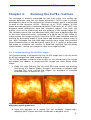
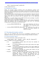
a. Open the map (starting fits file) with DS9 and choose the working
field using the Region shape “Polygon” and design a polygon that
includes the map cutting the edges. An example of possible
selected region is shown in Fig.1.
Fig.1 (I) Starting map (II) Starting map with the overlap of the selected
polygonial region (green line)
b. Save this polygon as a region file (for example “Region.reg”)
adopting WCS system and the coordinates in degrees units.
9
Cutex User’s Guide
d. Use the routine read_region (included in the CuTEx package) to load
the extremes of the chosen region
region = read_region(‘Region.reg’)
the region variable stores the coordinates of the polygon vertexes.
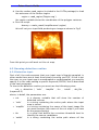
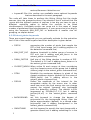
e. Run the script:
dummy = make_mask(‘mapfilename’,region)
this will cut your input field producing an image as shown in Fig.2
Fig.2 New cut image
From this point you will work on this cut map.
4.2 Running detection routine
4.2.1 Detection input
First of all, the code assumes that your input map is Nyquist sampled, in
other words there are at least three pixels covering your PSF. If that is not
the case, so your input map is oversampled or undersampled, you need to
specify it to the code setting a specific keyword (PSFPIX) that is described
in the next paragraph.
To launch the detection routine you must use the following syntax:
out = detection ( ‘indir’ , ’mapfile’ , thr , ’outdir’ , det_file ,
/keyword1-2)
where, in detail, the parameters are:
• out
• ‘indir’
• ‘mapfile’
• thr
• ‘outdir’
1
is a dummy variable that will store the number of
detected sources
is a string containing the entire path where the input
map is stored
is a string containing the name of the input image file
you want analyse (the name of the cut map if you have
do the preprocessing)
is a value that define the curvature threshold level to
identify the source candidates
is a string containing the entire path where all the
CuTEx User’s Guide
detection output will be stored
• det_file
is an IDL variable that will contain the name of the file
storing the list of detected sources and all the
parameters chosen to launch the detection tool.
• keyword1-2for this routine are available some optional keywords
that are described in the next paragraph.
4.2.2 Detection keywords
There are several option and keywords you can optionally activate for the
detection tool. A list of the useful keyword and their description is given
below:
• PSFPIX
expressing the number of pixels that sample the
PSF of the input image (set it adding psfpix=n in
the detection command line) (default 3)
• RANGE
number of pixels away from the candidate source
centre where to check the second derivative
minima (set it adding range=n in the detection
command line) (defaulf 9)
• NPIXMASK
a parameter that select the minimum number of
closest-neighbour pixels above the threshold to be
found to define a source candidate (set it adding
npixmask=n in the detection command line)
(default 4)
??? (set it adding /abscurve in the detection
command line)
the code use to default a threshold value constant
on all the image activating this keyword is possible
chose a method to calculate an adaptive threshold
depending on the local value of the curvature. (set
it adding /local_thresh in the detection command
line)
set this keyword to smooth the input image with a
gaussian kernel (set it adding smoothing=n in the
detection command line)
• ABSCURV
• LOCAL_THRESH
• SMOOTHING
4.2.3 How to use the keywords
In this paragraph we present some examples to explain “when and why”
you can use the detection keywords.
a) The use of PSFPIX and RANGE. The code is designed to work on
compact objects by removing, from the analysis, sizes that are larger
than 3 times the adopted PSF. For example, if in your map the PSF is
sampled by 7 pixels, a choice for the RANGE keyword should be about 20
pixels:
out = detection ( 'homedir/', 'mynicelookingmap.fits', 2.0,
'homedir/cutexoutput/', detectmymap, PSFPIX=7, RANGE=20 )
This will analyse the map 'mynicelookingmap.fits' in the directory
'homedir/' adopting a threshold of 2.0 times the rms of curvature of the
1
Cutex User’s Guide
map and will save the outputs in the directory 'homedir/cutexoutput/'.
b) The use of NPIXMASK. An important parameter that you can decide to
tune is the minimum size (the number of pixels) of contiguous pixels
above the threshold for defining a candidate. Such parameter is driven by
the variable NPIXMASK. The default value is 4. If from the inspection of
the first detection run on your map, you seems to be not identifying some
sources or there are a lot of contributions of spurious objects, please
check the mask fits files and change the NPIXMASK value. For example if
you are missing important sources that are covered by 3 pixels above
the threshold (you can see there is a clump of 3 pixels ruled out at the
detection stage) you can call:
out = detection( 'homedir/', 'mynicelookingmap.fits', 2.0,
'homedir/cutexoutput/', detectmymap, NPIXMASK=3)
In this way the threshold adopted will depend on the map you are
analysing and the same value of threshold will probably detect different
number of candidates on different maps.
c) The use of ABSCURV. This keyword is useful to determine the starting
threshold level. You can activate the ABSCURV to force the code to adopt
an absolute value for your curvature threshold, without depending on the
standard deviation of the map. We use such approach when we want to
rerun the detection on slightly different maps (processed with tiny
changes) adopting the same set up of parameters. For example
out = detection('homedir/', 'mynicelookingmap.fits', 22.5,
'homedir/cutexoutput/', detectmymap, /ABSCURV)
Will select all the pixels that have a curvature level along all the directions
above the value of 22.5. Keep in mind that in any case the absolute
curvature value will be saved in the header of the mask*.fits file
d) The use of LOCAL_THRESH. The use of LOCAL_THRESH keyword gives a
second method to determine the starting threshold level. LOCAL_THRESH
uses of an adaptive threshold depending on the local values of the
curvature. Using this approach, the code will compute locally the Median
Absolute Deviation (MAD - the median of the deviation from median
value) of the curvature in windows wide 61x61 pixels wide, for every
derivative map, along every different direction. Our tests indicate that the
MAD is the more reliable estimator to get less effected by the presence of
strong peaked sources on smooth backgrounds. Adopting this adaptive
approach, the probability to detect sources in cases of low emission
backgrounds is increased without increasing also the number of the
candidates/artefacts detected on bright emission regions. The maps of
local threshold have to be computed only one time. If the code finds
already those maps in the output directory for the detection routine, it will
not recomputed them. For example:
out = detection('homedir/', 'mynicelookingmap.fits', 22.5,
'homedir/cutexoutput/', detectmymap, /LOCAL_TRESH)
Will compute 4 different maps (one for each direction) where the values of
the local thresholds are saved in each pixel position. You can find those
maps called as, for example for one of the direction:
1
CuTEx User’s Guide
der2x_"nameofyourmap"_median.fits
in the output directory.
4.2.4 Detection outputs
There are several output products from the detection routine. The
derivate in several direction are stored in der*.fits and allder*.fits files,
some mask files containing the pixels found about the curvature threshold
level in mask*.fits.
The detected sources will be listed in the source*dat file, however this file
will not be useful to read. Nevertheless the detection routine produce
region files with the position and the guessed size of the detected
sources.
There are 3 *.reg file. Please load in DS9 the file sources_image_*.reg that
display the sources in image coordinate.
If you put as input a map called “DUMMYMAP.fits”, and choose a threshold
NNN, the detection will be produced output files with the following
nomenclature (listing here only the dat files) :
•
•
sources_NNN_DUMMYMAP.dat
The usual detection list but in
IPAC table (in the following called
sourcelist)
sources_NNN_DUMMYMAP_ellipse.dat
An additional file used to
estimate the guess ellipses at
detection stage.
4.3 Running photometry routine
Once you are satisfied with the list of candidates produced by the
detection routines, you can pass to fit them through Gaussian functions.
4.3.1 Extract_photo input
To call the extraction routine you have to run
extract_photo, ‘indir’ , ’mapfile’ , ’outdir’ , det_file , /keyword1-2
where, in detail, the input parameters are:
• out
• ‘indir’
• ‘mapfile’
• ‘outdir’
• det_file
is a dummy variable that will store the number of
detected sources
is a string containing the entire path where the input
map is stored
is a string containing the name of the input image file
you want analyse (the name of the cut map if you have
do the preprocessing)
is a string containing the entire path where all the
detection output will be stored
is an IDL variable that will contain the name of the file
storing the list of detected sources and all the
parameters chosen to launch the detection tool. To
restore the content of this variable from the last
detection section you previously run you can do
1
Cutex User’s Guide
restore,filename=’detection.sav’
• keyword1-2for this routine are available some optional keywords
that are described in the next paragraph.
The code will take times to perform the fitting, fitting first the single
sources, then the grouped sources. Pay attention that if noticed that the
group with the highest number of sources is too big you have to use a
different matching radius to define the sources to be fitted
simultaneously. Unreliable results can come out in the cases of large
number of gaussians fitted simultaneously. If your group size is too big try
using the keywords MAX_DIST_FAC to determine a smaller size for
grouping, as explain below.
4.3.2 Extract_photo keywords
There are several keywords you can optionally activate for the extraction
tool. A list of the useful keyword and their description is given below:
• PSFPIX
expressing the number of pixels that sample the
PSF of the input image (set it adding psfpix=n in
the detection command line)
• MAX_DIST_FAC
distance threshold to define group of sources in
PSF unit (set it adding max_dist_fac=n in the
extract_photo command line)
• DMAX_FACTOR
Half size of the fitting window in number of PSF.
The default is 2.0 (set it adding dmax_factor=n in
the extract_photo command line)
• CLOSEST_NEIGH When active fit each source at time considering
only the closest sources of the group (set it adding
/closest_neigh in the extract_photo command line)
• DTRH
• PSFLIM
• BACKGROUND
• SMOOTHING
1
Establish the maximum distance in pixels of the
closest neighbour objects (default it's the same of
DMAX_factor) (set it adding dtrh=n in the
extract_photo command line)
Define the amplitude of the interval for the
acceptable values for the source size. In other
word how much the final source size can change
respect the original "guessed" size (estimated
from the detection routine). The default is 30%
(expressed as PSFLIM=[0.7,1.3] (set it adding
psflim=[n1,n2] in the extract_photo command
line)
set this keyword to change the degree of
polynomial for the background fitting, from the
planar approximation (default) to a second order
polynomial. (set it adding /background in the
extract_photo command line)
set this keyword to smooth the input image with a
gaussian kernel (set it adding smoothing=n in the
CuTEx User’s Guide
extract_photo command line)
4.3.3 How to use the keywords
In this paragraph we present some examples to explain “when and why”
you can use the detection keywords.
a) The use of PSFPIX. The extraction routine needs to be informed of the
number of pixels that sample the PSF. Like detection routine it uses the
PSFPIX keyword to determine such a number of pixels.
b) The use of MAX_DIST_FACT. If your group size is too big try using the
keywords MAX_DIST_FAC to determine a smaller size for grouping. For
example:
extract_photo, 'indir, 'mapfile','outdir',detectionlistvariable,
MAX_DIST_FAC=1.5
Will group up sources that are closer than 1.5 times the PSF each other.
c) The use of DMAX_FACTOR. The gaussian fitting will be done on a
subframe centred on the single source / the barycentre of the group of
source. We found that the size of the fitted window is a critical parameter
for the fitting engine while fitting the background + the sources. In Hi-GAL
map we adopted as size of the fitting window a square of size
(2x(2*PSF(in pixels))+1)x(2*(2*PSF(in pixels)+1)). You can enlarge the
size of the subimage adopted for the fitting by setting the keyword
DMAX_FACTOR. In case you change it to N the fitting window will be
(Nx(2*PSF)+1)x(N*(2*PSF+1). Keep in mind that enlarging the window the
code might be slightly slower. However, it is very important to define the
right size of the fitted subimage on your own maps. Example of enlarging
the window:
extract_photo, 'indir, 'mapfile','outdir',detectionlistvariable,
DMAX_FACTOR=3.0
d) The use of CLOSEST_NEIGH and DTHR. A different approach (described
in the paper Molinari, et al. 2011) is included to define subgroups of
sources in the defined group to be simultaneously fitted to determine only
the flux of the central source. In other words, cycling on the sources
belonging to the same group, we select the subsample of sources falling
within the assumed cut-off length from the considered source. This
method is applied activate the CLOSETS_NEIGH keyword. For example, it
may happen that source C for example is associated with source A even if
the distance of C from A is larger than the assumed length of cut off. This
happen because to properly determine the flux of source B (the one
associate with A and C) you need to fit simultaneously A + B + C. Thus it
will fit at the same time the fluxes of the source A, B, C fitting 3 elliptical
gaussians simultaneously, assuming the same planar background for all
the sources. Instead, applying the CLOSEST_NEIGH method, the code will
fit first source A and its closest neighbour (the source B in the example
above). Then it will fit the source B through three gaussians (source
A+B+C - but will store only the flux for the source B in this case), then the
source C. This approach could in principle increase the number of fitting
steps to be followed, but improve a lot the performance of the code in the
1
Cutex User’s Guide
very crowded regions where a large number of sources could be grouped
together, with problems on the computational time but also on right
convergence of the fitting engine. You can set up the distance of cut-off
for the definition of each subgroup within a group adopting the keyword
DTHR. To follow this approach you have to call the routine with:
extract_photo, 'indir, 'mapfile','outdir',detectionlistvariable,
/CLOSEST_NEIGH, DTHR=3
The use of DTHR is optional, if you no set it the code use the default
value.
e) The use of PSFLIM. A critical keyword is the keyword PSFLIM. It defines
the interval of variation to be analysed respect the guessed size during
the fitted gaussian. In other words the extraction routine will get the
guessed size from the candidate source list and try the elliptical gaussians
with x / y sigma within an interval centred on the guessed size and going
toward the solution with the minimum chi square. By default the code
defines this interval as [0.7,1.3]*Guessed Size. Hence, during the fitting
process the size parameters will be varied inside such an interval.
WARNING: Please pay attention if after the fitting process the final
solution is equal to one of the limits of the interval. Unreliable fits could
come out if the gaussian fitting converges toward the maximum/minimum
of the intervals. If that is the case it may be possible that the code could
be converge to a better solution (smaller chi^2) if left free to vary on a
larger interval. Such aspect could be really tricky to verify. Keep in mind
that there could be a sort of quantization of the input/output size due to
this process.
At the detection level we estimate the source sizes from the position of
the curvature minima in the derivate maps. We determine such minima
and then fit an ellipse. For some reasons it can happen that the estimate
of one of the two ellipse's axis are smaller than the expected diffraction
limited PSF for the map you are analysing. In such case we force that axis
to be equal to the PSF. When this happen we put a flag in the detection
file equal to -1 (the column fitflag in the file generated by the detection).
In other cases it can happen that both the FWHM are pretty large (we
putted a constrain to 3 times the PSF) or that it is not possible to estimate
a proper ellipse fitting. In those cases we adopt as a guessed size a
slightly elongated source with sizes FWHM_X = PSF (in pixels) and
FWHM_Y = 1.1*PSF (in pixels) and we set the fitflag equal at 0. This
means that there are some FWHM values that occur often in the
candidate list produced by the detection.pro and such recurrence could
propagate to the output of the extraction process. We found that
sometimes the fitted gaussian (following an approach that minimize the
Chi square) is converging to unrealistic solutions (very big ellipses). Since
we have not developed the fitting engine, but used the Markwaldt's
approach it is not easy to control such cases. For this reason we
constrained the fit to not vary the sizes for more than 30% respect the
original values. We found from simulation that such interval define a good
compromise between size recovering and converging fit. However, when
we apply to Hi-GAL data, we found that we had to sometimes change the
1
CuTEx User’s Guide
size of the interval for the source size. To change the extreme of this
interval you could use the keyword PSFLIM. This is a keyword that accept
as values a two-element array. The two numbers define the limits of the
interval respect the guessed value that are probed during the fitting
process. For example:
extract_photo, 'indir, 'mapfile','outdir',detectionlistvariable,
PSFLIM=[0.5,2.0]
In other words, assuming that the source has a guessed size of fw_x = 4
and fw_y 4.4 (in pixels unit) and you set the PSFLIM keyword to “PSFLIM =
[0.5,2.0]“ it means that the fitting engine will fit elliptical gaussians with
sizes between ("0.5 * 4 =") 2 and ("2 * 4 =") 8 pixels for x direction and
("0.5 * 4.4 =") 2.2 and ("2. * 4.4 =") 8.8 pixels for the y direction.
Obviously during the fitting process it is not allowed to the gaussian to
have one of the axis smaller than the PSF size. The enlargement of the
fitting limits most of the times do not change the output results for the
fitted source if not that the fitting engine during the fitting process
converged at one of those limits (creating an over population of sources
at some size values).
f) The use of BACKGROUND. We also allow a different degree of
polynomial for the background. Our simulations and early studies indicate
that for small fitting window the planar approximation for the background
could be enough ( flux_background = A*x(pixel) + B*y(pixel) + C).
However, on HI-GAL maps with the large contribution of extended
emission a better estimate for the background might be a second order
polynomial (flux_background = A*x(pixel)^2 + B*y(pixel)^2 +
C*x(pixel)*y(pixel)^2 + D*x(pixel) + E*y(pixel) + F ). To enable the code
to evaluate the background with this approximation, please use the
keyword BACKGROUND. For example:
extract_photo, 'indir, 'mapfile','outdir',detectionlistvariable,
/BACKGROUND
4.3.4 Extraction outputs
If you put as input a map called “DUMMYMAP.fits”, Extract_photo will
produce the following files with this nomenclature:
• DUMMYMAP_photall.dat
the finaloutput file
• DUMMYMAP_photall_err.dat ??? Same as CuTEx 0.98
• DUMMYMAP_sdev.dat
??? Same as CuTEx 0.98
• DUMMYMAP_parameters.dat ??? Same as CuTEx 0.98
• DUMMYMAP_backpar.dat
????
1
Cutex User’s Guide
Chapter 5.
Output description
In this section the principal outputs of the detection and extraction
routines are described.
5.1 Detection output table
The detection main output (source*.dat) is a table in IPAC table format. An
interesting feature of the released CuTEx version is that in file of the
sourcelist above the IPAC table header it is saved a string containing the
exact command with which the current detection list was generated. It is
useful to recreate the same exact results once again.
The tags of the IPAC table produced by detection are:
• ID
• X
• Y
• X_AXIS
• Y_AXIS
• PA
• FIT_FLAG
• RA
1
INTEGER - is an increasing number that identified
the detected source
INTEGER - is the x coordinate of the source in the
image unit (pixel)
INTEGER - is the y coordinate of the source in the
image unit (pixel)
FLOAT - is a dimension of the ellipse (estimated
with the use of the first minima) along the x-axis
FLOAT - is a dimension of the ellipse (estimated
with the use of the first minima) along the y-axis
FLOAT - is the orientation angle of the major axis of
the ellipse respect to the x-axis
INTEGER - This is a flag that report on the elliptical
fit done on the minima of second derivate in the
attempt to establish a guess for the size of the
source. The possible values of the flag are:

-9
Elliptical Fit failed because there
were not enough pixels to evaluate the
fit

1
Elliptical Fit successful and
values are acceptable

0
Two possibility: (a) Source is
near a border so no attempt to establish
the size are done (please check also
BORDER_FLAG),
(b)
Elliptical
Fit
successful but values are larger than 3
times the PSF in pixels

-1
Elliptical Fit successful but the
FWHM of the X axis is smaller than the
PSF so it reported to the PSF value

-2
Elliptical Fit successful but the
FWHM of the Y axis is smaller than the
PSF so it reported to the PSF value
DOUBLE - is the right ascension of the detected
source in degree
CuTEx User’s Guide
• DEC
DOUBLE - is the declination of the detected source
in degree
• RA_STRING
STRING - is a string contain the RA value in
HH:MM:SS.SS
• DEC_STRING
STRING - is a string contain the DEC value in
DD:MM:SS.SS
• BORDER_FLAG INTEGER - This is a flag that report if the source is
too close to the border for CuTEx to perform its
analysis along all the direction. Basically if a peak of
curvature is detected nearby the border of the
image two things can happen:
 The source is in a pixel where the values of
second derivative might be influenced by
border effects (closer than 4 pixels to the
border)
 The source is in a pixel where it was not
possible to extract a subregion large enough
to determine the guess of the size (closer
than RANGE+3 pixels to the border). RANGE
can be set by a keyword, but if not set is
equal to 8 pixels.
Any border source is not fitted by the extraction
routine. The flag is equal 1 if the source is tagged
as border source, 0 if it is a valid source.
• CLUMP_FLAG
INTEGER - A flag that is different than zero if this
source belong to a clump of pixels for which it was
possible to determine multiple peak of curvature.
Since it happens that lowering the threshold limit
we identify larger groups of contiguous pixels
above such threshold this FLAG keep track if the
source is inside a larger clump. Multiple source with
the same values of this flag belong to the same
clump
• DIST_FLAG
INTEGER - A flag that contain a value from 0 to 3.
Floating point precision. This is the distance
between the pixel (C) with the maximum of
curvature (identified as the position in the detection
source list) and the pixel with maximum in intensity
(F) in a array 5x5 pixels centred around (C). During
the extract_photo this flag is read and the value
inside is adopted as maximum allowed distance
over which the centre of the fit can vary.
• GUESS_FLAG
INTEGER - A flag that is a number between 0 and 8.
Usually the numbers should be greater than 4. This
number counts the accepted positions used to
estimate the initial guess ellipse. Lower values of
this flag means a less reliable initial estimate for
the ellipse. Remember that for each direction
(maximum 4) there are two possible points in such
estimate
1
Cutex User’s Guide
• NAN_FLAG
• DER2X
• DER2Y
• DER2X45
• DER2Y45
• DER2X_THR
• DER2Y_THR
• DER2X45_THR
• DER2Y45_THR
INTEGER - A flag between 2 and 4. This is the
number different direction along which it was found
that the value of the derivative exceed the adopted
threshold. This value should be 4 for all the sources
except the one that nearby the NaN pixels, for
which this constrain is slightly relaxed. The sources
nearby NaN are usually listed in the end of the
sourcelist
FLOAT - is the value of the measured second
derivatives at the position of the maximum of
curvature alone the x direction
FLOAT - is the value of the measured second
derivatives at the position of the maximum of
curvature alone the y direction
FLOAT - is the value of the measured second
derivatives at the position of the maximum of
curvature alone the direction of a 45 degree
bisector
FLOAT - is the value of the measured second
derivatives at the position of the maximum of
curvature alone the direction of the other 45 degree
bisector
FLOAT - is the value of the adopted threshold
second derivatives at the position of the maximum
of curvature alone the x direction. This value will be
the same for all the sources if you are not using the
/LOCAL_THRESH keyword
FLOAT - is the value of the adopted threshold
second derivatives at the position of the maximum
of curvature alone the y direction. This value will be
the same for all the sources if you are not using the
/LOCAL_THRESH keyword
FLOAT - is the value of the adopted threshold
second derivatives at the position of the maximum
of curvature alone the direction of a 45 degree
bisector. This value will be the same for all the
sources if you are not using the /LOCAL_THRESH
keyword
FLOAT - is the value of the adopted threshold
second derivatives at the position of the maximum
of curvature alone the direction of the other 45
degree bisector. This value will be the same for all
the
sources
if
you
are
not
using
the
/LOCAL_THRESH keyword
5.2 Extraction output table
In the finaloutput, like in the sourcelist, you will find before the header of
the IPAC table a string containing the set up of parameters with which
that extraction was performed. Some Flags are repeated from the
2
CuTEx User’s Guide
DETECTION list file. This is intended to allow an easier read of those
values instead of digging out two files.
The tags of the IPAC table produced by Extract_photo are:
• ID
• X
• Y
• RA
• DEC
• GLON
• GLAT
• WAVELENGHTS
• F_PEAK
• FWHM_X
• FWHM_X
• PA
• F_INT
• ERR_F_INT
• BACK_ONPEAK
• RMS_ON
• RMS_OFF
• CHI2
• SIZE_FLAG
INTEGER - is an increasing number that identified
the detected source
INTEGER - is the x coordinate of the source in the
image unit (pixel)
INTEGER - is the y coordinate of the source in the
image unit (pixel)
DOUBLE - is the right ascension of the detected
source in degree
DOUBLE - is the declination of the detected source
in degree
DOUBLE - is the galactic longitude of the detected
source in degree
DOUBLE - is the galactic latitude of the detected
source in degree
FLOAT - the wavelength (as recognized by CuTEx)
in micron
FLOAT - is the peak flux of sources in the image
unit
FLOAT - is the Full Width Half Maximum of the
fitted bi-dimensional Gaussian along the x-axis
FLOAT - is the Full Width Half Maximum of the
fitted bi-dimensional Gaussian along the y-axis
FLOAT - is the orientation angle of the major axis
of the gaussian respect to the x-axis
FLOAT - is the integrated flux of the source in Jy
FLOAT - is the error of the integrated flux
FLOAT - is the background computed with the
assumption
of
planar/quadratic
background
estimated at peak position
FLOAT - is the RMS of the residual pixel fluxes
after the subtraction of the best fit to the initial
data. The RMS is computed only considering
PIXELS that are inside the fitting window but not
belong to the OTHER sources that might be
present. This means that pixels that belong to the
analysed source contribute to the estimate of the
RMS.
FLOAT - is the same of RMS_ON with the difference
that the estimate of the RMS value is done over all
the pixels inside the fitting window that not belong
to any sources.
FLOAT - is the sum of the residuals, it is not the
real chi^2 for which you need an error to weight
during the sum.
STRING - is a string flag that tell you if during the
2
Cutex User’s Guide
• GROUP_FLAG
• GAUSS_FLAG
• CLUMP_FLAG
• DIST_FLAG
• GUESS_FLAG
• STATUS
2
fitting procedure the output size converged to the
maximum or minimum allowed value (as default
we constrain the sizes to notary more than 30%
respect the initial guess). The string can contains
multiple tags:

+XU/+YU means respectively that the
size of X/Y converged to the maximum
allowed value possible

+XL/+YL if they converged to the
minimum allowed value

XPSF/YPSF If the size is constrained to
the PSF (or 0.95 times it)
INTEGER - is a progressive number, if analysed
source belong to a group this number will be
different from zero, all the sources with the same
value of this group are fitted together. Beware: If
you are using the keyword /CLOSEST_NEIGH this
flag is meaningless.
INTEGER - contains the number of gaussians used
at the same time during the fitting process
INTEGER - A flag that is different than zero if this
source belong to a clump of pixels for which it was
possible to determine multiple peak of curvature.
Since it happens that lowering the threshold limit
we identify larger groups of contiguous pixels
above such threshold this FLAG keep track if the
source is inside a larger clump. Multiple source
with the same values of this flag belong to the
same clump
INTEGER - A flag that contain a value from 0 to 3.
Floating point precision. This is the distance
between the pixel (C) with the maximum of
curvature (identified as the position in the
detection source list) and the pixel with maximum
in intensity (F) in a array 5x5 pixels centred
around (C). During the extract_photo this flag is
read and the value inside is adopted as maximum
allowed distance over which the centre of the fit
can vary.
INTEGER - A flag that is a number between 0 and
8. Usually the numbers should be greater than 4.
This number counts the accepted positions used to
estimate the initial guess ellipse. Lower values of
this flag means a less reliable initial estimate for
the ellipse. Remember that for each direction
(maximum 4) there are two possible points in such
estimate
INTEGER - is a status flag reported by MPFIT
engine. If this number is negative or zero
something is wrong in the fit result. If it is 5 this
CuTEx User’s Guide
• FIT_FLAG
• D2XDET
• D2YDET
• D2X45DET
• D2Y45DET
• D2XTHR
• D2YTHR
• D2X45THR
means that the maximum number of iterations
have been reached
INTEGER - This is a flag that report on the elliptical
fit done on the minima of second derivate in the
attempt to establish a guess for the size of the
source. The possible values of the flag are:

-9
Elliptical Fit failed because there
were not enough pixels to evaluate the
fit

1
Elliptical Fit successful and
values are acceptable

0
Two possibility: (a) Source is
near a border so no attempt to establish
the size are done (please check also
BORDER_FLAG),
(b)
Elliptical
Fit
successful but values are larger than 3
times the PSF in pixels

-1
Elliptical Fit successful but the
FWHM of the X axis is smaller than the
PSF so it reported to the PSF value

-2
Elliptical Fit successful but the
FWHM of the Y axis is smaller than the
PSF so it reported to the PSF value
FLOAT - is the value of the measured second
derivatives at the position of the maximum of
curvature alone the x direction
FLOAT - is the value of the measured second
derivatives at the position of the maximum of
curvature alone the y direction
FLOAT - is the value of the measured second
derivatives at the position of the maximum of
curvature alone the direction of a 45 degree
bisector
FLOAT - is the value of the measured second
derivatives at the position of the maximum of
curvature alone the direction of the other 45
degree bisector
FLOAT - is the value of the adopted threshold
second derivatives at the position of the maximum
of curvature alone the x direction. This value will
be the same for all the sources if you are not using
the /LOCAL_THRESH keyword
FLOAT - is the value of the adopted threshold
second derivatives at the position of the maximum
of curvature alone the y direction. This value will
be the same for all the sources if you are not using
the /LOCAL_THRESH keyword
FLOAT - is the value of the adopted threshold
second derivatives at the position of the maximum
2
Cutex User’s Guide
• D2Y45THR
• D2XFITDET
• D2YFITDET
• D2X45FITDET
• D2Y45FITDET
• D2XFITBCKDET
• D2YFITBCKDET
2
of curvature alone the direction of a 45 degree
bisector. This value will be the same for all the
sources if you are not using the /LOCAL_THRESH
keyword
FLOAT - is the value of the adopted threshold
second derivatives at the position of the maximum
of curvature alone the direction of the other 45
degree bisector. This value will be the same for all
the sources if you are not using the
/LOCAL_THRESH keyword
FLOAT - is the value of the second derivative
computed on the result of the FIT but IN THE
POSITION of the MAXIMUM OF CURVATURE. So this
is the contribution to the value of the derivative
that would have been measured produced by only
by the source (well the gaussian that best
reproduce the data fluxes). It is calculated alone
the derivative x direction
FLOAT - is the value of the second derivative
computed on the result of the FIT but IN THE
POSITION of the MAXIMUM OF CURVATURE. So this
is the contribution to the value of the derivative
that would have been measured produced by only
by the source (well the gaussian that best
reproduce the data fluxes). It is calculated alone
the derivative y direction
FLOAT - is the value of the second derivative
computed on the result of the FIT but IN THE
POSITION of the MAXIMUM OF CURVATURE. So this
is the contribution to the value of the derivative
that would have been measured produced by only
by the source (well the gaussian that best
reproduce the data fluxes). It is calculated alone
the derivative direction of a 45 degree bisector
FLOAT - is the value of the second derivative
computed on the result of the FIT but IN THE
POSITION of the MAXIMUM OF CURVATURE. So this
is the contribution to the value of the derivative
that would have been measured produced by only
by the source (well the gaussian that best
reproduce the data fluxes). It is calculated alone
the derivative direction of the other 45 degree
bisector
FLOAT - is the contribution to the second
derivative computed in the maximum of the
curvature produced by the fitted background.
Obviously in the case of planar background those
numbers will be all zero. It is calculated alone the
derivative x direction
FLOAT is the contribution to the second derivative
CuTEx User’s Guide
•
•
•
•
•
•
•
•
•
•
computed in the maximum of the curvature
produced by the fitted background. Obviously in
the case of planar background those numbers will
be all zero. It is calculated alone the derivative y
direction
D2X45FITBCKDET
FLOAT - is the contribution to the second
derivative computed in the maximum of the
curvature produced by the fitted background.
Obviously in the case of planar background those
numbers will be all zero. It is calculated alone the
derivative direction of a 45 degree bisector
D2Y45FITBCKDETFLOAT - is the contribution to the second
derivative computed in the maximum of the
curvature produced by the fitted background.
Obviously in the case of planar background those
numbers will be all zero. It is calculated alone the
derivative direction of the other 45 degree
bisector
D2XFITPEAK
FLOAT - is the same of D2XFITDET but calculated
in THE POSITION OF THE CENTER OF FITTED
SOURCE
D2YFITPEAK
FLOAT - is the same of D2YFITDET but calculated
in THE POSITION OF THE CENTER OF FITTED
SOURCE
D2X45FITPEAK FLOAT - is the same of D2X45FITDET but
calculated in THE POSITION OF THE CENTER OF
FITTED SOURCE
D2Y45FITPEAK
FLOAT is the same of D2Y45FITDET but
calculated in THE POSITION OF THE CENTER OF
FITTED SOURCE
D2XFITBCKPEAK FLOAT - is the same of D2XFITBCKDET but
calculated in THE POSITION OF THE CENTER OF
FITTED SOURCE
D2YFITBCKPEAK FLOAT is the same of D2YFITBCKDET but
calculated in THE POSITION OF THE CENTER OF
FITTED SOURCE
D2X45FITBCKPEAK
FLOAT - is the same of D2X45FITBCKDET but
calculated in THE POSITION OF THE CENTER OF
FITTED SOURCE
D2Y45FITBCKPEAK
FLOAT - is the same of D2Y45FITBCKDET but
calculated in THE POSITION OF THE CENTER OF
FITTED SOURCE
2
Cutex User’s Guide
Chapter 6.
Bibliography
− Faustini, Fabiana, Sergio Molinari, Leonardo Testi, e Jan Brand, A&A,
n. 503 (2009): 801.
− Hillenbrand, F.B. Introduction to Numerical Analysis. 1956.
− Lada, e Lada, ARA&A, n. 41 (2003): 133.
− Molinari, S., et al, PASP, n. 122 (2010): 314.
− Molinari, Sergio, Eugenio Schisano, Fabiana Faustini, Michele
Pestalozzi, A.M. Di Giorgio, e S.J. Liu, A&A, n. 530 (2011): 133.
− Testi, Leonardo, Francesco Palla, e A. Natta, A&A, n. 133, (1998):
81.
− Testi, Leonardo, Francesco Palla, T. Prusti, A. Natta, e S. Maltagliati,
A&A, n. 320 (1997): 159.
− Traficante, A., et al. MNRAS, n. 416 (2011): 2932.
2