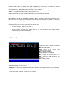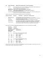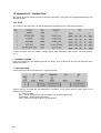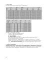
1
Observing at Medicina with ESCS 0.3 Name Authors Righini S (IRA) Orlati A (IRA) Bartolini M (IRA) Date 13/12/13 1 DOCUMENT CHANGE RECORD Issue date No. of pages 01 11/12/13 45 02 13/12/13 45 Issue No. 2 Pages changed, added, deleted Description of change Issue 01 Correction of errors, insertion of page numbers, addition of CalibrationTool as data writer 1 OVERVIEW AND SUMMARY ................................................................................................................................ 4 1.1 GLOSSARY: TERMS AND ABBREVIATIONS ...................................................................................................................... 5 2 OBSERVATIONS STARTUP .................................................................................................................................... 6 2.1 LOGIN ................................................................................................................................................................... 6 2.2 ON-‐SITE OBSERVATIONS ........................................................................................................................................... 6 2.2.1 escsRemote: input terminal and system monitors ...................................................................................... 6 2.2.2 escsConsole: access to schedules, logs and data ........................................................................................ 7 2.3 REMOTELY CONTROLLED OBSERVATIONS ...................................................................................................................... 7 3 INITIAL SETUP ...................................................................................................................................................... 8 4 ANTENNA OPERATIONS ....................................................................................................................................... 9 5 FRONTEND OPERATIONS ................................................................................................................................... 10 6 BACKEND OPERATIONS ..................................................................................................................................... 11 7 COMMAND-‐LINE MEASUREMENTS AND ACQUISITIONS .................................................................................... 12 7.1 7.2 7.3 7.4 7.5 7.6 RAW COUNTS READOUT ........................................................................................................................................ 12 TSYS .................................................................................................................................................................. 13 WEATHER PARAMETERS ........................................................................................................................................ 13 MANUAL ACQUISITIONS ........................................................................................................................................ 13 SKYDIPS ............................................................................................................................................................. 15 CAVEAT ON OFFSETS ............................................................................................................................................. 15 8 GENERATING AND LAUNCHING A SCHEDULE ..................................................................................................... 16 9 DATA FORMATS AND ONLINE QUICK-‐LOOK ....................................................................................................... 17 9.1 IF WRITER IS MANAGEMENT/FITSZILLA ................................................................................................................ 17 9.2 IF WRITER IS MANAGEMENT/POINT OR MANAGEMENT/CALIBRATIONTOOL ............................................................ 18 10 RETRIEVING THE DATA .................................................................................................................................... 19 11 REAL-‐LIFE EXAMPLE: CHECKLIST FOR ON-‐SITE CONTINUUM SCHEDULE-‐BASED OBSERVATIONS ....................... 20 12 APPENDIX A – MONITOR PANELS FULL DESCRIPTION ...................................................................................... 21 12.1 12.2 12.3 12.4 12.5 12.6 12.7 OPERATORINPUT ................................................................................................................................................ 21 ANTENNABOSS .................................................................................................................................................. 21 OBSERVATORY ................................................................................................................................................... 23 MOUNT ........................................................................................................................................................... 23 GENERICBACKEND ............................................................................................................................................. 24 RECEIVERSBOSS ................................................................................................................................................. 25 SCHEDULER ....................................................................................................................................................... 25 13 APPENDIX B – COMPLETE COMMAND LIST ...................................................................................................... 26 14 APPENDIX C – SCHEDULE STRUCTURE .............................................................................................................. 29 14.1 SCAN-‐SUBSCAN OBSERVATIONS ............................................................................................................................. 29 14.2 SCHEDULE FILES ................................................................................................................................................. 30 14.2.1 SCD file ................................................................................................................................................... 30 14.2.2 LIS file ..................................................................................................................................................... 33 14.2.3 CFG file ................................................................................................................................................... 37 14.2.4 BCK file ................................................................................................................................................... 38 14.2.5 DAT file .................................................................................................................................................. 39 15 APPENDIX D – OUTPUT FILES ........................................................................................................................... 40 15.1 FITS ................................................................................................................................................................ 40 15.2 MBFITS .......................................................................................................................................................... 43 16 APPENDIX E – SOURCE CATALOGUE ................................................................................................................. 45 3 1 Overview and summary ESCS (Enhanced Single-dish Control System) is the control software produced for the Medicina and Noto radiotelescopes. It is a distributed system based on ACS (ALMA Common Software), commanding all the devices of the telescope and allowing the user to perform single-dish observations in the most common modes. As of today, the code actually implemented for the telescopes (i.e. excluding the huge ACS framework) amounts to more than 468.600 lines (about 397.00 if not considering comments). This guide is meant to help the observer in the use of ESCS, without dealing with the “behind-the-curtains” complex details of the system. This release focuses on single-dish continuum observations, as the only fully integrated backend available on-site is the analogue total power one. Since both the hardware and software implementations are still going on, this manual will forcibly undergo continuous revisions. Here follows a simple schematization of the observing system, helpful to visualize all the main devices ESCS deals with and the most important operations it performs. Notice: the features not yet available in this release are shown in brackets. Antenna 4 DEVICES: mount subreflector Frontend DEVICES: Primary Focus: X band receiver Cassegrain Focus: C band receiver and K band dual-‐feed receiver Backend DEVICES: TotalPower (XARCOS spectrometer) "Back door" for guest backends OPERATIONS: readout and command of all the devices OPERATIONS: Frequency setup, calibra`on mark switching OPERATIONS: For fully integrated backends: device setup and data collec`on Observing modes Beam parking, sidereal tracking, posi`on switching, (nodding), (frequency switching), raster scan/map, On-‐The-‐Fly scan/map Data format OUTPUT FILES including readouts from weather sta`on: (MBFITS) -‐> included but not fully tested FITS ASCII for calibra`on tools 1.1 Glossary: terms and abbreviations Beam-parking the antenna points to a fixed Azimuth-Elevation position Bin FWHM frequency channel Full-Width Half-Maximum HPBW Nodding Half-Power BeamWidth (aka “beam switching”) it involves two or more feeds. The source is alternatively observed with each of the feeds, so that there is always one feed “on source” OTF On-The-Fly acquisition. The antenna moves according to user-defined parameters, scanning the sky at constant speed. Data acquisition is active during the scan Position switching (aka “on-off”) the beam is alternatively pointed to the source (on) and to a properly defined offset position (off) Preset mount mode allowing only beam-parking observations, with no pointing model applied ProgramTrack Raster mount mode allowing tracking, OTF/raster scans, beam-parking with pointing model corrections acquisition is performed via discrete pointings (in tracking or beam-parking mode), planned to sample a certain path/area on the sky Section acquisition stream (aka “logical channel”). E.g.: the 2-feeds of the K-band dual-feed receiver used with the continuum backend produce 2 feeds x 2 polarizations = 4 sections SF Slewing Single-Feed motion of the antenna when it is going to the target position. Slewing is performed at maximum speed, with no data acquisition taking place Time-tagged commands the positions commanded to the antenna are all associated to a time tag, so that the execution of the operations is always time-dependent. Command lines can be temporized as well, indicating a specific UT date-time for the launch of the command itself TPB Tracking TotalPower backend the antenna points to the target and follows its sidereal motion 5 2 Observations startup Login 2.1 àNotice: login and password are provided locally to each project. As the control room logistics might undergo updates, be sure to contact the local staff before your session starts, in order to get the latest information. Observations involve the use of two machines, located in the 32-m dish control room (the one storey building beside the antenna): 2.2 Login: projectName Login: observer Use for: • schedulecreator; • access to data, schedules, logs; • IDL, including the FITS quicklook procedure and SDI (a map-making tool); • DS9 and FV for FITS viewing. Use for: • all ESCS-related operations; • instrumentation setup; • launching/stopping schedules; • quick-look of non-FITS data. On-site observations When the observers perform their acquisitions on-site, they exploit the escsConsole machine only - the one on the left. From there, a VNC connection (see details in the following sub-section) leads to escsRemote. 2.2.1 escsRemote: input terminal and system monitors Login to escsConsole using your projectName. Then, click on the VNC icon located on the Desktop. It will connect you to escsRemote as “observer” On escsRemote, you should find the input terminal and all the monitors already running. If, instead, you need to start them, open a terminal on escsRemote and give: > escsClients This opens 8 panels at once: • • • • • • • • 6 operatorInput - terminal for command line input antennaBoss observatory mount genericBackend receiversBoss scheduler logging Rearrange the panels on the virtual desktop. In case any of them does not automatically start, you can manually open them by means of individual command lines, to be given in the open terminal: > operatorInput > antennaBossTui > observatoryTui > mountTui > genericBackendTui BACKENDS/TotalPower (or other backend code) > receiversBossTui > schedulerTui > loggingDisplay à All the antenna/receiver/backend setup procedures are performed via the operatorInput window, which is also used to start/stop the schedules. The other panels are monitors used to display a vast amount of information, see Appendix A – Monitor panels full description and Appendix B – Complete command list for a comprehensive description of their content and a list of all the commands available for the operatorInput (they can be inserted in schedules as well). 2.2.2 escsConsole: access to schedules, logs and data Directly use escsConsole for the data quicklook and retrieval (see dedicated sections), for the generation of schedules using schedulecreator and for tools as DS9 or FV. Login credentials are specific to each project. Once logged in, in your home you can find the following folders, whose names are self-explanatory: ~/data ~/schedules ~/logs à Note on schedules: users can generate subfolders according to their needs to store their schedules, but, in order to be executed, schedules must be places exactly in the ~/schedules folder. 2.3 Remotely controlled observations It is possible to remotely perform the observations, exploiting a VNC connection to escsRemote. Open a VNC session and connect to 192.167.189.57:2 (i.e. port 5902) You will be asked to insert a password, which is the same used locally to login to escsRemote with the observer user. If you need to start the clients, open a terminal and command: > escsClients and follow the same instructions provided for observations carried out on site. To access the other machine (escsConsole), where your data, schedules and logs are stored, simply open a terminal on your computer and use > ssh –X [email protected] Hence you can launch IDL, use schedulecreator, retrieve your data, etc… 7 3 Initial setup When opening an ESCS observing session, it is necessary to perform a setup which includes the antenna unstow and its configuration in tracking mode. This is done by means of a unique command, which is specific for the wanted receiver, to be written in the operatorInput. The currently available choices are: > setupXXP > setupCCC > setupCCCL > setupKKC for the X band receiver (Primary focus) for the C band receiver (Cassegrain focus) for the C band receiver (Cassegrain focus), using the narrow band (see below) for the K band dual-feed receiver (Cassegrain focus) à General info: spaces within the command line content are not allowed! The above setup command sets the antenna mount, the minor servos, the selected receiver and the default backend (TotalPower) according to default parameters. The antenna mode is set to ProgramTrack (allowing tracking and the execution of schedules), while the Local Oscillator frequency and the bandwidth are set as illustrated in the following table. àNotice: any time the mount mode is switched to ProgramTrack, the antenna will slew and go to the position which had been observed the last time the ProgramTrack was active. This is normal, you can command a different target or go on with other operations. Receiver CCCL CCC XXP KKC LO freq (MHz) 4600 4600 8080 21964 Frontend IF band (MHz) 100 - 250 100 - 900 100 - 900 100 - 2100 Backend IF band (MHz) 50 - 250 50 - 780 50 - 780 50 - 2400 Observed bandwidth (MHz) 150 680 680 2000 Observed band (MHz) 4700 - 4850 4700 – 5380 8180 – 8860 22064 - 24064 Notes 1 – Fixed value: there is no tunable LO for this receiver. Notice that, depending on the devices in use, the sky frequency at the observed band starting point is given by the LO frequency plus an offset. For the present combinations of the frontends with the total power backend, which the above table refers to, this offset is 100 MHz. In general, the true observed band depends on the intersection between the frontend IF band and the chosen backend filter. The actual observed bandwidth and the band starting frequency are recorded in the output files (see Appendix D – Output files). The default logfile is named station.log. If the user wants to change it: > log=logfilename (without extension) Logfiles are stored in a dedicated folder (see Retrieving the data). When schedules are run, a new logfile is automatically started, and it is named after the schedule: schedulename.log. It is possible, and advisable, to insert the project code/name (a string assigned to the project by the TAC, the same you use as a login name on escsConsole) using the command: > project=projectName This will make the user save time in later stages, as it will not be necessary to specify the project name in schedule-launching commands. The project code/name must correspond to an existing user, already known to the system. This means that, if its spelling does not match with the recorded name, an error rises. 8 4 Antenna operations Note on the format for coordinates. Whenever celestial coordinates (Equatorial, Horizontal or Galactic) are specified, the allowed formats are: - decimal degrees, using a ‘d’ suffix, for any coordinate à e.g. 30.00d - sexagesimal degrees, with no suffix, for any coordinate à 30:00:00 - hh:mm:ss, with a ‘h’ suffix, for longitudes only à 02:00:00h (not accepted for offsets) Besides the overall telescope setup previously described, individual commands are available to change the antenna mount status and manage its steering/pointing: > antennaUnstow it only performs the unstow procedure > antennaSetup=CCC (or other receiver code) it unstows the antenna (if it is stowed) then it sets the pointing model and the minor servo system according to the selected receiver. Mount is set to ProgramTrack mode > antennaTrack it sets the mount to ProgramTrack mode, allowing the execution of sidereal tracking, on-off, OTF scans, etc… Even beam-parking acquisitions (i.e. on a fixed Az-El position) can be now performed in ProgramTrack mode by means of the goTo command > track=sourcename if the antenna is in ProgramTrack mode and the sourcename is known within the station catalogue (which includes the most commonly observed calibrators), it directly points to the source and tracks it e.g. > track=3c286 > sidereal=sourcename,RA,Dec,epoch,sector if the antenna mode is ProgramTrack, it points to the supplied RA-Dec position and temporarily assigns the sourcename label to it. Epoch can be ‘1950’, ‘2000’ or ‘-1’, the last one meaning that the provided coordinates are precessed to the observing epoch. The sector keyword forces the cable wrap sector, if needed: its value can be ‘cw’, ‘ccw’ or ‘neutral’. The last option means the system will automatically choose the optimal alternative. e.g > sidereal=src12,319.256d,70.864d,2000,neutral > goOff=frame,offset it slews the antenna to an offset position, in the indicated coordinate frame (‘eq’, ‘hor’ or ‘gal’). The user provides the offset value (degrees only), but the system automatically chooses on which axis to perform the slewing, taking into account the present position of the antenna e.g. > goOff=eq,1.0d > azelOffsets=azoff ,eloff it sets user-defined offsets in the Horizontal frame (degrees only) e.g. > azelOffsets=0.5d,0.3d sets an azimuth offset to 0.5 degrees and the elevation offset to 0.3 degrees > radecOffsets=raoff ,decoff it sets user-defined offsets in the Equatorial frame (degrees only) e.g. > radecOffsets=0.3d,0.0d sets the right ascension offset to 0.3 degrees and the elevation offset to 0.0 degrees > lonlatOffsets=lonoff ,latoff it sets user-defined offsets in the Galactic frame (degrees only) e.g. > lonlatOffsets=0.1d,0.5d sets the galactic longitude offset to 0.1 degrees and the galactic latitude offset to 0.5 degrees à NOTE on offsets: these user-defined offsets are the overall antenna offsets and they are mutually exclusive! If the user commands the offsets several times in a row (in one or different frames) only the last one will be effective. Offsets specified within schedules, at subscan level, sum up to these user-defined offsets. 9 > goTo=Az,El it points the antenna to fixed Az-El positions e.g. > goTo=180d,45d > antennaStop it stops the antenna motion, if any, and changes the mount mode to Stop > antennaPark it stows the antenna 5 Frontend operations To change the frontend Local Oscillator frequency, use the following command: > setLO=freq1;freq2;…;freqN notice the semicolon. Ideally, different values could be assigned to different IFs, thus tuning each section to a different sub-band. For the present hardware, though, this is not possible, so a single value must be specified: e.g. > setLO=4900 Remember that the actually observed band begins at a frequency which is usually different from the LO one (see Initial setup) à The X band receiver is not provided with a tunable Local Oscillator, and the observed RF band is fixed. The temperature of the calibration mark in use is recorded in the logfile whenever a Tsys is measured. It is also stored in the FITS/MBFITS output files. The calibration mark can be manually switched on and off respectively with: > calOn > calOff If the user wants to perform the setup for the frontend only (without affecting the mount, the minor servo or the backend), the command is: > receiversSetup=CCC (or other receiver code) 10 6 Backend operations Important note: the TotalPower backend works as a “focus selector”, sending the signal from the wanted receiver to any other backend. For this reason, it must be set up even when acquisitions take place using another backend. This is accomplished simply using the overall setup commands (such as setupCCC, etc…). The backend to be used can be manually selected as follows: > chooseBackend=BACKENDS/bckname where bckname is the name of the backend. At present, the only available choice is: TotalPower Bandwidth and sampling rate can be changed using: > setSection=sect,startFreq,bw,feed,mode,sampleRate,bins where sect is an integer specifying the section number startFreq is the initial frequency for the section (not applicable for TPB) bw is a double for the bandwidth (MHz) feed is the number of the feed connected to the section (not applicable for TPB) mode is the polarization mode (not applicable for TPB) sampleRate is also given in MHz bins is the number of frequency bins for the given section (not applicable for TPB) To leave a parameter at its previously set value, or equivalently skip it when it is not applicable, use ‘*’. For the TPB, in particular, always use: > setSection=sect,*,bw,*,*,sampleRate,* where bw can be chosen from a restricted range of options (MHz): 300.0 730.0 1250.0 2000.0 These values do not correspond to the true observed bandwidth, for the reason discussed in Initial setup. When accumulations of the data “dumps” are required before integrating them to the output file, it is possible to set the integration time as follows: > integration=N where N is given in milliseconds. With > getTpi you can measure the raw counts level of the signal. The returned value includes the backend zero-level (Tp0, around 200 counts), while your data will be recorded as Tpi-Tp0. Each section is provided with an attenuator, to manage the signal intensity. To set the desired attenuation: > setAttenuation=sect,att where sect is the section number and att can vary, for the TPB, form 0 dB to 15 dB, with a 1 dB step. The signal level should be around 900 counts for Elevation=45°. 11 As the signal level equalisation among all the sections is usually desired, and the number of sections is quite high when using multi-feed receivers, it is possible to save time using the following command: > agc=BACKENDS/bckname,desired_tpi where desired_tpi is the signal level (in raw counts) to be reached. An iterative procedure will take place; it will configure each attenuator in order to get signal levels as near as possible to the desired one. à Note: the procedure can take up to 30 seconds. Furthermore, if the signal power is too low or too high to be equalised with the available attenuations, the process will not be successful. For these reasons, it is not advised to use agc inside schedules. If a backend re-initialization is needed, use > initialize=CCC (or other code) This command resets the backend only, setting it to the default values foreseen for the specified focus/receiver. After the frontend/backend configuration is changed, it is necessary to update the value for the beamsize (HPBW), which is computed as a function of the actually observed band and is used – during the observations – to evaluate the pointing accuracy. This is accomplished using the command: > device=sect which uploads to the system the parameters relative to section number sect (you can generally use 0, which exists for all the receivers, unless you need to observe only with a different feed). 7 Command-line measurements and acquisitions Once the system and telescope setup had been completed, it is possible to manually perform measurements and observations, which might as well pave the way – as preliminary checks – to longer lasting sessions carried out via schedules. 7.1 Raw counts readout The raw counts readout (called Tpi) of the signal can be obtained with > getTpi The system reply consists in an array of values (one for each section). As concerns the TPB, it is important to ascertain that the Tpi lies within the 800-1000 counts range – this is the linear region for the backend. If this requirement is not met, it is necessary to iteratively vary the attenuation for the needed sections and check the Tpi, until the signal intensity falls into the proper range. As the signal level greatly varies with elevation, it is advisable to perform this operation in the elevation range that will be actually exploited during the observations or, as a general rule, at elevation=45°. Of course, the signal level is also greatly affected, especially at high frequencies, by weather conditions, therefore the attenuation tuning should be carried out again every time the conditions change. When you are going to manually get the Tpi - in order to ascertain which attenuation values to use in your schedule - remember to set the LO frequency and the bandwidth as they will be employed in the schedule. After a setup command, in fact, they are set to defaults; instead, if a schedule has been previously run, these values remain set as indicated in the last schedule reading. 12 7.2 Tsys To measure the Tsys value: > tsys the system replies with N values, where N is given by the total amount of (input_lines x sections). When using the TotalPower backend, N is the number of sections (2 for single-feed receivers and 4 for the dualfeed receiver). àNOTICE: the last measured Tsys value will be stored in the system and used, if the FITS format is selected for data storage (Appendix D – Output files), to get a counts-to-Kelvin conversion factor, in turn applied to all the following acquisitions, until a new Tsys is measured. The FITS file will contain the raw data (in counts) and also a table with the data stream calibrated (in K) using this counts-to-Kelvin factor. 7.3 Weather parameters The weather station measurements can be retrieved with: > wx the reply will list ground temperature (°C), relative humidity (%), atmospheric pressure (hPa), wind speed (km/h). Updated values are available every 10 seconds. 7.4 Manual acquisitions When performing manually commanded acquisitions, it is necessary to select the recording device: > chooseRecorder=string where string can be: MANAGEMENT/FitsZilla MANAGEMENT/MBFitsWriter MANAGEMENT/Point MANAGEMENT/CalibrationTool if FITS output is desired if MBFITS is preferred (not yet tested) (default) text output in the logfile, used for pointing calibration text output in the logfile, used for pointing calibration (details will be provided once this feature is fully tested) Once the recorder is set, acquisitions on a target can be performed as follows. First, set the target: > track=sourcename (if the source is included in the system catalogue, see Appendix E) or > sidereal=sourcename,RA,Dec,epoch,sector (see Antenna operations) Then, command cross-scans across the target: > crossScan=subscanFrame,span,duration where subscanFrame is the coordinate frame along which the scan is performed (‘eq’, ‘hor’ or ‘gal’), span is the spatial length on sky of the individual subscan (i.e. one line of the cross) expressed in degrees, duration is the time length espressed in hh:mm:ss, e.g. > crossScan=eq,1.0d,00:00:30 corresponds to one cross-scan carried out in Equatorial coordinates (one line along RA, one line along Dec), each line being 1° in span. Each subscan lasts 30 seconds, thus the resulting scan speed is 2 °/min. When the MANAGEMENT/Point writer is used, the cross-scan produces text output in the logfile only (no output file is recorded). This output text contains information obtained by the automatic processing of the subscans. In particular, a Gaussian fit is performed in order to measure the source position and estimate the pointing offsets. If the fitting procedure in successful and the achieved offsets are considered plausible, pointing corrections are immediately applied. This means that, if no user-defined offset is commanded afterwards, the measured offsets remain active and are applied to the following observations. 13 Here follows the function that is separately fitted to latitude and longitude subscans: W y(x)=A*e + ax +c where 2 W = -2.7725887 * F F = (x-µ)/FWHM µ = abscissa of peak The results are given in the logfile, in the following sequence of lines: LATFIT latoff fwhm A a c i LONFIT lonoff fwhm A a c i OFFSET avlon avlat lonoff latoff lonflag latflag XOFFSET avlon avlat lonoff*cos(lat) latoff lonoff_err latoff_err lonflag latflag XGAIN target avlon avlat lonampl lonampl_err latampl latampl_err lonFWHM lonFWHM_err latFWHM latFWHM_err flux lonflag latflag Where (all angles in degrees): latoff = latitude offset lonoff = longitude offset i = number of iterations performed by the fitting procedure avlon = average longitude of peak (in same coordinate frame as the subscan execution) avlat = average latitude of peak (in same coordinate frame as the subscan execution) lonflag = fit result for longitude subscans (1 = plausible fit, 0 = non plausible fit, -1 = fit did not converge) latflag = fit result for latitude subscans (1 = plausible fit, 0 = non plausible fit, -1 = fit did not converge) lonoff_err = error on longitude offset latoff_err = error on latitude offset target = target name lonampl = amplitude measured on longitude subscans (K) lonampl_err = error on amplitude measured on longitude subscans (K) latampl = amplitude measured on latitude subscans (K) latampl_err = error on amplitude measured on latitude subscans (K) lonFWHM = FWHM measured on longitude subscans lonFWHM_err = error on FWHM measured on longitude subscans latFWHM = FWHM measured on latitude subscans latFWHM_err = error on FWHM measured on latitude subscans flux = catalogue target flux (Jy), if available (otherwise it is put to 0.0). à Notice: it is possible to include scans using the MANAGEMENT/Point writer in schedules as well. For example, an improved pointing can be achieved setting the first scan on a source as a /Point scan, then the following scans (e.g. producing FITS/MBFITS files) will hold the offsets optimising the pointing, given that no user-defined offset is updated by means of an explicit radeOffsets, azelOffsets or lonlatOffsets command. 14 7.5 Skydips Skydip scans are indispensable in order to characterize the atmosphere. They consist in moving the telescope along a vast span in elevation (at fixed azimuth) while sampling with a backend. Their analysis allows the user to quantify the atmosphetic opacity τ. There are different ways to perform this: > skydip=El1,El2,duration e.g. skydip=80d,20d,00:05:00 performs a skydip between 20 and 80 degrees (at the current azimuth position), the scan will take 5 minutes (speed is 12 °/min). The arguments must be in the range 0-90. The jolly character is supported for the elevation arguments. Example: skydip=*,*,00:04:00 will perfom the skydip between the default values for elevation (15° and 90°). Please notice that pointing corrections are disabled. Since no backend recording is automatically enabled by this command, remember to activate the FitsZilla recorder – as explained in § 7.4 – before launching the command, in order to save the data! This command can be used within schedules as well. See Appendix C for details. 7.6 Caveat on offsets As seen in Antenna operations, there are commands used to set (or null) user-defined offsets. They are: radeOffsets, azelOffsets and lonlatOffsets. Such commands set overall offsets which remain active until they are explicitly changed/nulled by another call of one of the three commands. Further offsets, having for example the purpose of pointing the antenna to an off-source position, are specified inside schedules, at the subscan level (see Appendix C – Schedule structure). These subscan-level offsets sum up to the overall offsets, and they are zeroed by default every time a new subscan is commanded. 15 8 Generating and launching a schedule A schedule is a set of files where all the geometry/timing/frequency details of a sequence of data acquisitions are specified, according to a syntax that enables ESCS to read and execute them. The detailed structure of the several files composing a schedule is explained in Appendix C – Schedule structure. Schedules for the most common observing modes (OTF cross-scans and maps, raster maps and ON-OFF) can be easily produced using a tool called schedulecreator. See its documentation for details. Once a schedule is ready, it must be copied to the folder reserved to the project (/home/schedules). There, the schedule formal consistency can be tested using the scheduleChecker command given within a terminal: > scheduleChecker schedname.scd Only the syntax correctness will be verified. If errors are present, a reply will briefly address them indicating their position inside the files. To launch a schedule, simply use: > startSchedule=projectName/schedname.scd,N projectName is the unique string assigned to every project. It can be omitted if the project command had been used. If both the choices are made, i.e. if the project name was set with project but a string is also inserted in the startSchedule command, the latter overrides the former. Then follows the schedule name, in particular the name of the SCD file. N is the identifier of the scan or subscan from which ESCS must start reading it – it is particularly useful in case of a sequential (i.e. not time-based) schedule. “N” can be the scan number, e.g. 2, or the scan_subscan specification, e.g. 2_5. You can specify when to start the schedule (in UT): > startSchedule=projectName/schedname.scd,N@DOY-HH:MM:SS ESCS reads the configuration parameters from the schedule, which can be relative both to the receiver and the backend, and accordingly sets these devices. This might take a few seconds, especially when using the dual-feed receiver. While the setup takes place, several values change in the TPB monitor. The last operation is the upload of the first pointing/scan read from the schedule, whose parameters will show up in the bottom section of the AntennaBoss monitor. During the scans, all the three flags in the lower part of the AntennaBoss monitor must be a green @ . Pay attention to the Tracking one. It should turn to a red o only when the antenna is slewing between scans on the same source, or when slewing to/from a new source. If tracking is not correct for some consecutive seconds during a scan, something is wrong. Sequential schedules run ad libitum. To abruptly interrupt the running schedule, truncating the ongoing acquisition: > stopSchedule Instead, to stop the schedule allowing the completion of the present file: > haltSchedule 16 9 Data formats and online quick-look 9.1 If writer is MANAGEMENT/FitsZilla Open a terminal on escsConsole. When acquiring FITS files through a schedule, there is an IDL tool available for the semi-realtime quicklook of the saved data. Launch IDL: > idl > idlde (for the command-line version, to be preferred) or (for the graphic interface) At the IDL prompt, compile and run the program fits_look.pro IDL> .r fits_look IDL> fits_look The last available FITS file will be plotted. Full usage: IDL> fits_look [,pin=] [,x=] [,y=] [,/help] where: pin = full path to data storage folder (the one containing the scan subfolders) x = letter indicating the choice for the x-axis label, default is 's' y = choice of the data stream, default is 'raw', displaying raw counts, while using 'atemp' the antenna temperature - if available* - is shown. The procedure iteratively lists all the folders in the given path pin and displays on screen the Feed0L and Feed0R data of the last surely complete FITS file recorded in the last written folder (see picture below). If pin is not provided, the path to the data is by default to the folder where data is currently being written. The x-axis can be represented as sample number (if x='s'), elapsed time from the acquisition start (if x='t'), azimuth degrees (if x='a'), elevation degrees (if x='e'), declination degrees (if x='d'), right ascension hh.hhh (if x='r'). Default is SAMPLE NUMBER. Please report any problem/request about this tool, as it is very basic and still under development. * The antenna temperature data streams are available only if a Tsys has been correctly acquired prior to the execution of the scan. See Appendix D for details. 17 9.2 If writer is MANAGEMENT/Point or MANAGEMENT/CalibrationTool When data are acquired – both manually or through a schedule – using the Point or CalibrationTool writers, the quick-look must be performed using the CalibrationToolClient. Open a terminal on escsRemote and use the command: > calibrationtoolclient componentName where componentName is either MANAGEMENT/Point or MANAGEMENT/CalibrationTool. A graphic window will appear. Its content is given in the following figure. Notice that, in this client, the subscan currently being acquired is shown in real-time (upper plot), even if in a low-res version. Under this display, the last completed subscan, in its full sampling, is shown. 18 10 Retrieving the data Open a terminal on escsConsole. Your data folder is ~/data/ its subfolders are named according to the date (YYYYMMDD) will be automatically created during acquisitions. Taking into account the choice of the FITS format, the only one so far fully tested, the date-dependant folder contains a subfolder for every scan, inside which there are the FITS files (one for each subscan): MainFolder |-----> YYYYMMDD | |-----> Scan1Folder | | |-----> Subscan1.FITS | | |-----> Subscan2.FITS | | | |-----> Scan2Folder | |-----> Subscan1.FITS | |-----> Subscan2.FITS | |-----> YYYYMMDD |-----> Scan1Folder | |-----> Subscan1.FITS | |-----> Subscan2.FITS | |-----> Scan2Folder |-----> Subscan1.FITS |-----> Subscan2.FITS FITS filenames are composed as: YYYYMMDD-HHMMSS-projectName-Suffix where HHMMSS is the UT time associated to the first sample of the acquisition projectName is the code/name specified using the “project=” command, or when starting a schedule with “startSchedule=projectName/schedulename.scd,N” Suffix is a user-defined string retrieved from the schedule files. Though no control can be applied on the choice/check of this string, the agreement is that it must coincide with the target name. à Notice: acquisitions performed manually (i.e. from command line, not through a schedule) are all stored into ~/extraData 19 11 Real-life example: checklist for on-site continuum schedule-based observations (1) = action to be performed on the observing machine (escsRemote) (2) = action to be performed on the data-access machine (escsConsole) (O) = command to be given in the operatorInput Login (2,1) Login on (2) using your projectName Using the VNC icon on the Desktop, connect to (1) as “observer”. Launch the monitors, if necessary (1) ☐ escsClients Setup (O) ☐ setupCCC (or other receiver code) Tune the local oscillator, start frequency of the observed band will be 100 MHz higher ☐ setLO=freq (e.g. setLO=4900) Point the antenna to a reference position ☐ goTo=Azd,Eld (e.g. goTo=180d,45d) Measure the cold sky signal level + adjust attenuation until it is about 900 counts ☐ getTpi ☐ acg=BACKENDS/TotalPower,900 ☐ getTpi (to check whether the agc command was successful, otherwise set the attenuations manually until the signal level is about 900 counts) Get a Tsys ☐ tsys Create a schedule (2) Use schedulecreator (see its own guide) ☐ schedulecreator –c [configfile] [out_directory] Move the schedule files to the folder ~/schedules Check the schedule formal correctness ☐ scheduleChecker schedname.scd Launch the schedule (O) ☐ startSchedule=projectName/schedulename.scd,N Launch data quick-look (2) – if acquiring FITS files ☐ idl ☐ IDL> .r fits_look ☐ IDL> fits_look Stop the schedule (O) ☐ stopSchedule Copy the data (2) à Get the latest subfolders written in the ~/data folder Stow the antenna (O) ☐ antennaStop ☐ antennaPark Close the monitors, if necessary (1) ☐ escsClients --stop (individual panels can be closed typing “exit” in their command lines) 20 12 Appendix A – Monitor panels full description 12.1 operatorInput This is the input console where users write ESCS commands. The prompt is just a sequential number enclosed in <>. If a command is properly read, the system replies repeating the command itself, followed by the operation results (if they are foreseen). Otherwise, an error message appears. To close the window, type ‘exit’. 12.2 AntennaBoss This monitor shows the commanded and actual positions. It also gives a feedback on the pointing accuracy and on the overall antenna status. Parameters Target: label (as extracted from schedule), coordinates (RAJ2000.0, DecJ2000.0), VLSR (km/s, if available), estimated flux density (Jy, if available). Horiz. Offs: Horizontal (Az-El) offsets as read from schedule, degrees. Equat. Offs: Equatorial (RA-Dec) offsets as read from schedule, degrees. Galac. Offs: Galactic (l-b) offsets as read from schedule, degrees. Raw Horizontal: commanded Az-El, including pointing model, refraction, etc... Observed Horizontal: Az-El coordinates read from the mount encoders and cleaned from the pointing model and refraction contributions. Because of this, observed coordinates will differ from the raw ones. Observed Equatorial: RA-Dec J2000.0 coordinates, converted from the observed horizontal. Observed Galactic: l-b Galactic coordinates, converted from the observed horizontal. 21 Generator Type: which component is in charge of the generation of the coordinates. It can be NONE (which is the condition at startup), OTF, MOON or SIDEREAL. Corr. az/el/ref: azimuth and elevation corrections (degrees) applied by the pointing model, plus the refraction model contribution– which is an additional correction to elevation. FWHM: Full Width Half Maximum (corresponding to HPBW), degrees. Enabled: a green “@” indicates that the antenna is correctly receiving commands; a red “o” means the communication is disabled. Tracking: it indicates whether the pointing error exceeds 0.1*FWHM or not. A green “@” corresponds to error < 0.1*FWMH. It should turn to a red “o” only when the antenna is slewing between scans on the same source, or when slewing to/from a new source. Correction: application of the above horizontal coordinates corrections. If disabled (red circle), all corrections are zeroed. Status: OK, WARNING or ERROR. “Warning” needs investigation but usually does not stop the ongoing activity (it also appears at startup, before the setup commands), “Error” generally appears if something stops the observations. Generator: under this line all the subscan setup parameters appear when it is commanded. In particular, for OTF observations: Start-Center-Stop – coordinates in the subscan frame of the start, center and stop positions (degrees) StartTime-Dur. – subscan start UT (yyyy-doy-hh:mm:ss.s) and duration (hh:mm:ss.s) J2000-Apparent eq – during the subscan, current RA-Dec position pointed by the antenna, both in the J2000 epoch and precessed to the date. Format is hh:mm:ss.s-°°:’ ’:” ”.” Horizontal - during the subscan, current Az-El position pointed by the antenna (degrees) Galactic - during the subscan, current l-b position pointed by the antenna (degrees) Sky/Phi rate – actual subscan speed on sky along scanning direction (°/s). The ‘Phi rate’ value refers to great circle arcs, if it is the scanning geometry, otherwise it copies the first speed value. For SIDEREAL scans, instead, this is what appears: Source name –target name Catalog Eq. – target FK5 coordinates and info (if available): RA hh:mm:ss.s, Dec °:’:”.”, Epoch, RA proper motion (milliarcsec per julian year), Dec proper motion (milliarcsec per julian year), parallax (milliarcsec), radial velocity (km/s) Catalog Gal. – target Galactic longitude and latitude (degrees) converted from the above Equatorial or provided by user/catalogue Apparent Eq. – target current apparent Equatorial coordinates: RA hh:mm:ss.s, Dec °:’:”.”, Epoch Galactic – current l-b position pointed by the antenna (degrees) Horizontal –current az-el position pointed by the antenna (degrees) To close the monitor, type ‘exit’ in its prompt (the grey line). 22 12.3 Observatory It is devoted to the station coordinates and times. Observatory Name: SRT, Medicina or Noto Universal Time: YYYY-DOY-HH:MM:SS.SSS Julian Day: d.ddd Apparent GST: HH:MM:SS.SSS Greenwich Sidereal Time LST: Local Sidereal Time HH:MM:SS.SSS DUT1: difference between UT1 and UT (s), if applied. Pole motion: celestial pole offset w.r.t. a reference position (details are note provided here), measured in µarcsec on a tangential projection. Geodetic Coords: updated Latitude and Longitude (degrees) and Altitude (m) for the telescope, plus the geodetic model code. Geocentric Coords: geocentric cartesian coordinates (m) for the telescope. To close the monitor, type ‘exit’ in its prompt (the grey line). 12.4 Mount This is a quite complex frame, allowing the technical staff to monitor all the various parts of the antenna mount. Observers must focus only on a subset of the displayed parameters and flags. We thus describe the main features only. The top left section gives the online readouts for the Azimuth and Elevation axes, compared to the commanded positions. Line by line: Azimuth: current azimuth position (in the -90°/450° wrapping range), rate (°/s) and commanded offset (degrees). Then the measured position error and tracking error (both in degrees) are given. Finally, the axis active mode is displayed: it can be PRESET (fixed Az-El pointing only), PROGRAMTRACK (for tracking, OTF and schedules), STOP (if axes brakes are on), UNKNOWN (indicating a non-configured status). Cmd Az. : commanded azimuth position (in the -90°/450° wrapping range), rate (°/s) and offset (°). This offset comes from metrology devices, it is not related to user-defined offsets or subscan-defined offsets. 23 Elevation: current elevation position (degrees), rate (°/s) and commanded offset (degrees). Then the measured position error and tracking error (both in degrees) are given. Finally, the axis active mode is displayed: it can be PRESET (fixed Az-El pointing), PROGRAMTRACK (for OTF and schedules), STOP (if axes brakes are on), UNKNOWN (usually indicating an error condition). Cmd El. : commanded elevation position (degrees) and rate (°/s). Wrap: readouts from the cable wrap. The status flag on the right can be CW or CCW. The general condition of the mount is summed up by one keyword, in the central part: Mount status: it can be OK, WARNING, FAILURE or BUSY, the latter is associated to operations which take a lot of time to complete (as the stow-unstow procedure). When the mount is BUSY it will not accept further commands until the ongoing operation is completed. The rest of the panel lists several flags and status labels. For average users, the only points to be taken into account are: • in standard observing conditions, when a schedule runs, all flags should be green “o”; • in case of warnings, flags turn to yellow “o”; • errors correspond to red “o”; • when a “failure” keyword turns steadily to a red “o”, or a permanent failure status appears, immediately call for technical assistance. To close the monitor, type ‘exit’ in its prompt (the grey line). 12.5 GenericBackend The panel shows one row for every section. Freq: value (MHz) to be added to the LO frequency in order to obtain the observed frequency at the beginning of the band BW: bandwidth (MHz) Feed: number of the receiver feed connected to this section S.R.: sampling rate (MHz) Pol: polarization (Left or Right) Bins: number of frequency bins (1 for total power) DBs: attenuation (dB) applied to the section Sect: section number Tsys: the last measured Tsys (K) Also some backend-dependent status flags are present, in the top right area. When observing with the TPB, look for: Time_Sync: if it frequently or steadily turns red call for assistance (the backend time is not synchronized) Busy: when schedules are running, it must turn yellow. If it does not, the backend is not acquiring. To close the monitor, type ‘exit’ in its prompt (the grey line). 24 12.6 ReceiversBoss This monitor summarizes the frontend setup. Current setup: receiver code. Mode: NORMAL, SINGLEDISH, VLBI… (other codes to come). Status: OK, WARNING or FAILURE Feeds: number of feeds (1 fore single-feed receivers, 2 for the K-band dual-feed receiver) LO: Local Oscillator frequency (MHz) Start Freq.: step (MHz) to be added to the LO frequency in order to obtain the actually observed frequency at the beginning of the band Bandwidth: actually observed bandwidth (MHz) Polarization: LCP, RCP, HLP or VLP. To close the monitor, type ‘exit’ in its prompt (the grey line). 12.7 Scheduler This monitor shows details on the selected data acquisition devices and on the running schedule, if any. Project code: project name, as specified at the launch of the schedule (or as input using the project= command) Schedule: name of the active schedule Scan/Subscan: scan number and subscan number, relative to the ongoing acquisition Backend: name of the selected backend, as listed in the schedule Recorder: name of the selected data recording device, as listed in the schedule Device: number of the currently selected device (see device= command) Tracking: tracking status of the telescope, including antenna, active surface, minor servo. A red “o” means the telescope is not yet in its tracking route (or that it is not tracking properly), a green light means the observation is ongoing and the tracking is accurate within 0.1*HPBW Status: flag summarising the telescope status. OK is sel-explanatory, WARNING in principle indicates that the acquisition can go on even if a problem has been reported, ERROR signals that a major problem was detected and the observation cannot be performed. à Notice: all the monitors can be closed at a time using the command (in a terminal on the observing machine): > escsClients --stop 25 13 Appendix B – Complete command list NOTICE: all commands can be temporized adding a proper suffix. There are two possibilities: - absolute temporization (the operation will be performed at the indicated time) “@DOY-HH:MM:SS”, where DOY is the Day-Of-Year (1-366) and HH:MM:SS is the UT time; - iterative temporization (the operation is performed now, then periodically according to the indicated time interval) “@!DAYS-HH:MM:SS”, where DAYS is the number of days and HH:MM:SS is hours, minutes, seconds. Temporized commands can be used also in the init/POST-scan/post-scan procedures inside schedules. Observers are in charge of considering if and when the use of a certain command makes sense in their schedule, according to their specific needs and goals: this is something that no schedule parser can check! > agc=BACKENDS/bckname,desired_tpi sets the attenuations in order to reach, for all the active sections, a signal level as near as possible to the desired_tpi (raw counts). As the completion of the operations can take up to 30 seconds, the use of this command within schedules is not recommended. Example: acg=BACKENDS/TotalPower,850 > antennaPark sends the antenna to stow position > antennaSetup=code (CCB, KKG, ...) unstows the antenna, sets it to tracking mode and configures the pointing model according to the specified receiver. It does NOT perform the receiver and backend setup > antennaStop stops the antenna. Activities can start again only commanding a mode change as antennaTrack (which does not affect the overall setup) or a new setup > antennaTrack sets the antenna to PROGRAMTRACK mode. It does not change the pointing model or any receiver setup > azelOffsets=double’d’,double’d’ sets the Az-El offsets (degrees). They are intended “on sky” Example: azelOffsets=-0.05d,0.05d > calOn switches the calibration mark on > calOff switches the calibration mark off > chooseBackend=string BACKENDS/XARCOS selects the backend; string can be BACKENDS/TotalPower or > chooseRecorder=string selects the backend; string can be MANAGEMENT/FitsZilla, MANAGEMENT/MBFitsWriter or MANAGEMENT/Point > crossScan=scanFrame,span,duration performs a cross-scan on the previously selected target*, along the scanFrame (‘eq’,’hor’ or ‘gal’), spanning span degrees in duration seconds. * indicated using the track or sidereal commands > device=sect computes the beamsize, taking into account the present receiver and backend configurations relative to section sect > flush=N deletes the N-th element in the queue of temporized commands > flushAll deletes all the queue of the temporized commands > getAttenuations reads the attenuation values (dB) currently configured for the active sections, and lists them according to increasing section number > getTpi reads the signal intensity (raw counts) for the active sections, and lists them according to increasing section number > goOff=frame,offset slews the antenna to an offset position, in the indicated coordinate frame (‘eq’, ‘hor’ or ‘gal’). The user provides the offset value (degrees only), but the system automatically chooses on which 26 axis to perform the slewing, taking into account the present position of the antenna > goTo=double’d’,double’d’ sends the antenna, while in TRACKING mode, to the specified Az-El position. Example: goTo=180d,45d The arguments are always rounded in the range 0-360 and 0-90 for azimuth and elevation respectively (in any case the ranges are limited to mechanical contraints). The jolly character is valid and is considered as: keep the present value.The differences from the preset command are: 1) once the antenna reaches the destination, the system will acknowledge the “on source” status; 2) the pointing corrections (pointing model and refraction) are applyed. In case they are not required they must be turned off explicitly. > haltSchedule completes the current scan and then stops the schedule > initialize=code (CCB, KKG, etc...) configures the backend using the default parameters relative to the selected receiver. It does NOT act on the receiver, pointing model or antenna mount mode > lonlatOffsets=double’d’,double’d’ sets the Galactic b-l offsets (degrees). They are intended “on sky”. Example: lonlatOffsets=2.0d,-1.0d > moon points the antenna to the present coordinates of the center of the Moon > preset=double’d’,double’d’ sends the antenna, if in PRESET mode, to the specified Az-El position, without applying any pointing correction. This is useful when needing to point to a position next to the zenith. Beware: the antenna will reach the destination but no “on source” flag will be raised. Example: preset=180d,45d > project=code lets the system know which project is observing (the code/name must correspond to the one provided by the TAC). This code/name is then considered as default when launching schedules: the system will search for them in a folder named “project/schedules”. This code/name also forms part of the output FITS filename. Notice that the PROJECT keyword indicated inside the schedule, which is then written in the “Project Name” keyword in the FITS main header, is a free string and might differ from the project official name. > radecOffsets=double’d’,double’d’ sets the RA-Dec offsets (degrees). They are intended “on sky”. Example: radecOffsets=1.0d,0.0d > receiversMode=code configures the working mode of the receiver, according to its peculiar characteristics > receiversSetup=code (XXP, CCC, KKC) configures the receiver using the default parameters. It does NOT act on the backend, pointing model or antenna mount mode > setAttenuation=sect,att sets to att (dB) the attenuator of section sect > setLO=freq Local Oscillator frequency, in MHz (one per IF, separated by “;”, usually the values are identical) This LO frequency corresponds to: SkyFreq(@band start) – 100 MHz when using the TPB > setSection=sect,startFreq,bw,feed,sampleRate,bins configures the backend section sect. > setupCCC (setupKKC, etc…) unstows the antenna, sets it to tracking mode, selects the pointing model, and configures the receiver and the backend using default parameters. In practice, it is a shortcut corresponding to this sequence: antennaSetup=Code, receiverSetup=receiverCode, initialize=receiverCode, device=0, calOff > sidereal=sourcename,RA,Dec,epoch,sector points to the supplied RA-Dec position and temporarily assigns the sourcename label to it. Epoch can be ‘1950’, ‘2000’ or ‘-1’, the last one meaning that the provided coordinates are precessed to the observing epoch. The sector keyword forces the cable wrap sector, if needed: its value can be ‘cw’, ‘ccw’ or ‘neutral’. The last option means the system will automatically choose the optimal alternative. Example: > sidereal=src12,319.256d,70.864d,2000,neutral 27 > skydip=El1,El2,duration performs an OTF acquisition at the current azimuth position, spanning in elevation from El1 to El2 (both expressed in degrees, with ‘d’ suffix), in duration seconds. A recorded must have previously been enabled in order to save the data. > startSchedule=[project/]schedulename.scd,N runs schedule schedulename.scd (project is the ID of the observing project, it is optional if it has already been input through the projectNamecommand), reading it from line N > stopSchedule immediately stops the running schedule, truncating the acquisition > ti lists all the active temporized commands > track=sourcename points the antenna, in sidereal tracking, to the specified source, which must be present in the local catalogue. If you need to insert frequently observed sources in this catalogue, contact the system manager > tsys measures the system temperature (K) in the position the antenna is pointing to. It returns a list of values, one for each section in use (e.g. 4 values for the whole dual-feed receiver). All the intermediate steps and calculations are stored in the active logfile > wait=d.d sets a delay (in seconds) which is applied before the system reads/executes the next command > wx returns the current weather parameters: ground temperature (°C), relative humidity (%), atmospheric pressure (hPa), wind speed (km/h). 28 14 Appendix C – Schedule structure A schedule is a set of files where all the geometry/timing/frequency details of a sequence of data acquisitions are specified, according to a syntax that enables ESCS to read and execute them. In order to generate the schedules, for the most common observing modes in continuum and (partially) spectroscopy, a tool called Schedulecreator is available (see IRA Technical Report 266/13). For regular observations, users should not edit the schedule files: for most of the applications, they can totally ignore what is written inside them. Only expert users, wanting to customize their observations in unusual or complex ways, should access the schedules and edit them, or create schedules from scratch using their own tools. For this purpose, the following sections describe the general scheme conceived for the observations and the content of the files composing the schedule. 14.1 Scan-subscan observations We define the scans and subscans composing the observing session as follows: Scan It is the lowest level object normally used by an observer. It is a sequence of one or more subscans that share a single goal: for instance cross-scans and maps involve a pattern of subscans. Whether OTF maps mosaicing observations are considered a single scan or a series of scans is rather a matter of how the user would like to define it. In our implementation each map is considered a scan. Subscan it is the minimal amount of data acquisition that can be commanded at the script language level. It is highly desirable that it is a simple enough element. For example, it is the single OTF “line” of a map or of a crossscan. The figure below visually represents what cross-scans, OTF maps and raster maps are. In the case of cross-scan, a subscan is a single arrow (a line across the target), four arrows – i.e. two full crosses – constitute the schema which might be repeated as many times as needed within the scan. For OTF maps, the subscan is again the single arrow, and the scan coincides with the whole map obtained with lines along one axis only (e.g. along RA or Dec). For raster maps, which are based on discrete acquisitions, each point is a subscan, and the final map constitutes the scan. When choosing FITS as the data output format, a distinct FITS file is produced for each subscan listed in the schedule. The scan-subscan dependency is more evident when MBFITS are created, as the observation arrangements illustrated above reflect into a hierarchical structure for the several folders and files that constitute the MBFITS. Details on the file production are given in the next section, where the .scd component of the schedule is described. 29 14.2 Schedule files The present release of the system requires a 4+1 files: • .scd file: it holds the sequence of scans/subscans to be performed • .lis file: it lists the spatial configuration of the single subscans composing the observation • .cfg file: it contains the frontend configuration and other procedures to be used in the initialization phase (if any) and in the pre-scan/post-scan operations (if any). Any ESCS command can be inserted in these procedures. Users are warned, however, that their employment might not be necessarily useful: pay attention to the meaningfulness of their insertion within the schedules. • .bck file: it is devoted to the backend setup • .dat file: this file is used only in case the MBFITS output format is chosen, as it contains information that is not read by ESCS but is needed in the writing phase of the file. 14.2.1 SCD file This is the main schedule file, listing the scans/subscans to be executed. In case of a sequential schedule, scans/subscans are not associated to specific execution times, so they are carried out sequentially following an “as soon as possible” approach. Values are all TAB-separated. The header must contain the following keywords, including the final colon: PROJECT: OBSERVER: SCANLIST: PROCEDURELIST: BACKENDLIST: MODE: user-defined label for the project. It will end up in the output filename. name of the observer. It will end up in one FITS file header. name of the LIS file to be used. name of the CFG file to be used. name of the BCK file to be used. schedule mode: SEQ for sequential schedules, LST for time-based schedules. If SEQ, then a tab-separated start LST time can be specified as HH:MM:SS. If LST, then a tab-separated value can indicate how many times [INITPROC: [SCANLAYOUT: the schedule must be run name of the initialization procedure (contained in the CFG file), optional] name of the DAT file (for MBFITS only, otherwise it has no effect)] Then, the scans/subscans are listed. Each scan is introduced by a line starting with “SC:” followed by some scan-level information: 30 SC: Scan# ScanLabel BCKProcedure:WriterName [ScanLayoutName] Scan# is the number for the scan. It must be unique in the schedule. Scan numbers must be incremental but do not need to be sequential. ScanLabel will be included in the output filename. BCKProcedure is the name of a valid procedure listed in the BCK file. WriterName is the name of the output data writer (MANAGEMENT/FitsZilla or MANAGEMENT/MBFitsWriter). ScanLayoutName is the name of the layout selected from the DAT file. It should be omitted, as it is useless, when FITS files are chosen for data output. After the scan setup, all the subscans composing that scan are specified, like: Scan#_subscan# Duration Scan#_subscan# Duration SubscanID PreProcedure PostProcedure SubscanID PreProcedure PostProcedure is the sequential number for the subscan, e.g. 1_1, 1_2, etc… is the subscan duration (seconds). For OTF subscans it must coincide with the duration declared in the LIS file is the ID for the subscan to be executed, as reported in the LIS file is the name of the procedure, enclosed in the CFG file, to be performed in the POST-subscan phase. Parameters can be passed as name=value. is the name of the procedure, present in the CFG file, to be performed in the post-subscan phase. Parameters can be passed as name=value. Here follows an example of sequential schedule where the chosen output file format is FITS. PROJECT: Test3c295 OBSERVER: John Doe SCANLIST: Test3c295.lis PROCEDURELIST: Test3c295.cfg BACKENDLIST: Test3c295.bck MODE: SEQ INITPROC: INIT SC: 1_1 1_2 1_3 1_4 1_5 1 0.0 14.0 14.0 14.0 14.0 300_40 300_40:MANAGEMENT/FitsZilla 1 NULL POSTTSYS 5 NULL POST 6 NULL POST 7 NULL POST 8 NULL WAIT=1.0 SC: 2_1 2_2 2_3 2_4 2_5 2 0.0 14.0 14.0 14.0 14.0 730_20 730_20:MANAGEMENT/FitsZilla 1 NULL POSTTSYS 5 NULL POST 6 NULL POST 7 NULL POST 8 NULL WAIT=1.0 Please notice that sequential schedules run ad libitum, as long as the targets are above the horizon and the user does not input a stopSchedule command. 31 An equivalent schedule, this time for MBFITS output files, could be: PROJECT: Test3c295 OBSERVER: John Doe SCANLIST: Test3c295.lis PROCEDURELIST: Test3c295.cfg BACKENDLIST: Test3c295.bck MODE: SEQ INITPROC: INIT SCANLAYOUT: Test3c295.dat SC: 1_1 1_2 1_3 1_4 1_5 1 0.0 14.0 14.0 14.0 14.0 300_40 300_40:MANAGEMENT/MBFitsWriter scanLayout_0001_3C295 1 NULL POSTTSYS 5 NULL POST 6 NULL POST 7 NULL POST 8 NULL WAIT=1.0 SC: 2_1 2_2 2_3 2_4 2_5 2 0.0 14.0 14.0 14.0 14.0 730_20 730_20:MANAGEMENT/MBFitsWriter scanLayout_0002_3C295 1 NULL POSTTSYS 5 NULL POST 6 NULL POST 7 NULL POST 8 NULL WAIT=1.0 It is possible to write sidereal-time-based schedules, assigning the ‘LST’ value to the header keyword ‘MODE’, followed by the number of repetitions foreseen for the schedule (1 means that, when the schedule has completed one run, it stops). It is then necessary to add a column to the SCD file, where the LST start times for the individual subscans are provided. This feature is not included in the present release of the Schedulecreator, so this schedule version can be obtained only editing a sequential schedule, or using custom tools. The single subscan line then becomes: Scan#_subscan# StartLST Duration SubscanID Here is an example of time-based schedule: PROJECT: Test3c295 OBSERVER: John Doe SCANLIST: Test3c295.lis PROCEDURELIST: Test3c295.cfg BACKENDLIST: Test3c295.bck MODE: LST 1 INITPROC: INIT SC: 1_1 1_2 1_3 1_4 1_5 32 1 300_40 300_40:MANAGEMENT/FitsZilla 12:23:35.0 0.0 1 NULL POSTTSYS 12:23:40.0 14.0 5 NULL POST 12:24:00.0 14.0 6 NULL POST 12:24:20.0 14.0 7 NULL POST 12:24:40.0 14.0 8 NULL POST PreProcedure PostProcedure SC: 2_1 2_2 2_3 2_4 2_5 2 730_20 730_20:MANAGEMENT/FitsZilla 12:26:55.0 0.0 1 NULL POSTTSYS 12:27:00.0 14.0 5 NULL POST 12:27:20.0 14.0 6 NULL POST 12:27:40.0 14.0 7 NULL POST 12:28:00.0 14.0 8 NULL POST 14.2.2 LIS file This file lists all the spatial subscan configurations employed within the schedule, one for each line. They do not need to follow the execution sequence in which they are called by the SCD schedule: the first column gives a unique incremental ID (not necessarily sequential: gaps are allowed) to be included in the calls inside the SCD file. Fields are TAB-separated. # 3C295 1 SIDEREAL 2 SIDEREAL 3 SIDEREAL 4 SIDEREAL 5 OTF 3C295 6 OTF 3C295 7 OTF 3C295 8 OTF 3C295 TSys TSys TSys TSys 212.8360d 212.8360d 212.8360d 212.8360d EQ EQ EQ EQ 52.2025d 52.2025d 52.2025d 52.2025d 212.8360d 212.8360d 212.8360d 212.8360d 0.0d 0.0d 0.7d 0.7d 52.2025d 52.2025d 52.2025d 52.2025d 0.7d 0.7d 0.0d 0.0d 2000.0 2000.0 2000.0 2000.0 EQ EQ EQ EQ -EQOFFS -EQOFFS -EQOFFS -EQOFFS EQ EQ EQ EQ 0.0d 0.0d -0.35d 0.35d LON LON LAT LAT -0.35d 0.35d 0.0d 0.0d CEN CEN CEN CEN INC DEC INC DEC 14.0 14.0 14.0 14.0 -EQOFFS -EQOFFS -EQOFFS -EQOFFS 0.0d 0.0d 0.0d 0.0d 0.0d 0.0d 0.0d 0.0d Three different subscan types can be used: SIDEREAL, OTF, OTFC and SKYDIP. SIDEREAL subscans They are used for tracking and on-off acquisitions: the antenna points to the specified position. The LIS line is composed by: ID = unique ID for the subscan configuration TYPE = subscan type label, in this case ‘SIDEREAL’ TARGET = label for subscan target/content FRAME = frame for the coordinates to follow. Options: ‘EQ’, ‘HOR’ or ‘GAL’ LONGITUDE = target longitude, following the generally allowed longitude formats LATITUDE = target latitude, following the generally allowed latitude formats EPOCH = for EQ coordinates only. ‘-1’ means the coordinates are precessed to date. OFFSET LABEL = [opt] frame for the offsets to follow. Options: ‘-EQOFFS’, ‘-HOROFFS’ or ‘GALOFFS’ LON OFFSET = [opt] longitude offset (degrees, with ‘d’ suffix) LAT OFFSET = [opt] latitude offset (degrees, with ‘d’ suffix) à Notice: the offsets frame can be freely chosen, regardless of the frame describing the target coordinates. These offsets sum up to the overall offsets that might have been defined by the users with the radecOffsets, azelOffsets and lonlatOffsets commands. By default, subscan-level offsets are zeroed any time a new subscan is commanded, and new offsets (if any is specified in the LIS line) take over. Though the definition SIDEREAL clearly implies the tracking of a celestial source, a “degenerate” use of this subscan type is given by beam-parking observations: when users want to acquire data in a fixed Az,El position, they can use SIDEREAL subscans where the coordinate frame is ‘HOR’. Please notice that, though this observing mode implies no antenna motion, it fully corresponds to the execution of a schedule with scans/subscans as concerns data acquisition, so the mount must be in tracking mode (and not in preset mode) in order to perform this kind of observation. 33 OTF subscans On-the-fly subscans are paths on the sky run at constant speed while acquiring data. The LIS line is composed by: ID = subscan unique ID TYPE = subscan type, in this case ‘OTF’ TARGET = label for target LON1 = for DESCR=’SS’ (later keyword), longitude (*) of the scan starting point. For DESCR=’CEN’, longitude (*) of the subscan central point. LAT1 = for DESCR=’SS’ (later keyword), latitude (!) of the scan starting point. for DESCR=’CEN’, latitude (!) of the subscan central point. LON2 = for DESCR=’SS’ (later keyword), longitude (*) of the subscan ending point. for DESCR=’CEN’, whole longitude span (*) of the subscan. LAT2 = for DESCR=’SS’ (later keyword), latitude (!) of the subscan ending point. for DESCR=’CEN’, whole latitude span (!) of the subscan. FRAME = coordinate frame relative to the previously specified lon-lat coordinates: ‘EQ’ = Equatorial J2000.0 (longitude = RA, latitude = Dec) ‘HOR’ = Horizontal (longitude = azimuth, latitude = elevation) ‘GAL’ = Galactic (longitude = l, latitude = b) sFRAME = coordinate frame along which the scan is performed. It must be equal to FRAME, apart from a single case: if FRAME is ‘EQ’ and the scan description is ‘CEN’ (see next keywords), then sFRAME can also be ‘HOR’, which means that Az-El scans will be performed across a sidereal position. This is usually exploited for pointing calibration campaigns. GEOM = scan geometry: LON = constant longitude LAT = constant latitude GC = great circle arc (only for DESCR=’SS’) DESCR = scan description: SS = start and stop positions CEN = center position + scan span DIR = scan direction (ignored if GEOM=’CG’): INC = the varying coordinate increases DEC = the varying coordinate decreases DURATION = scan actual duration in seconds (acceleration/deceleration ramps excluded) offFRAME = [opt] frame for the user-defined offsets to be added to the lon-lat coordinates specified (the leading dash ‘ –‘ is compulsory): -EQOFFS = Equatorial -HOROFFS = Horizontal -GALOFFS = Galactic At present offFRAME must be equal to sFRAME, which means that it is not possible to perform scans in an exotic way like scanning along the galactic longitude while applying equatorial offsets, etc... but it is possible to apply Az,El offsets to Az,El scans across a sidereal (equatorial) position. LONOFF = [opt] longitude offset, in degrees, which can be specified as dd.dd’d’ (decimal format, can be positive or negative, notice the ‘d’ suffix) or dd:mm:ss.s. It is meant to be “on sky”, i.e. the actual span, in practice ∆lon x cos(lat). LATOFF = [opt] longitude offset, in decimal degrees (notice the ‘d’ suffix). à Notice: these offsets sum up to the overall offsets that might have been defined by the users with the radecOffsets, azelOffsets and lonlatOffsets commands. By default, subscanlevel offsets are zeroed any time a new subscan is commanded, and new offsets (if any is specified in the LIS line) take over. 34 Examples of valid OTF subscans: 1 2 3 4 OTF OTF OTF OTF Source1 Source1 Source2 Source3 310.256d 310.256d 12:45:12h 21.738d 30.231d 30.231d 18:12:21.1 88.205d 310.256d 0.0d 0.7d 0.7d 30.931d 0.7d 0.0d 0.0d EQ EQ EQ GAL EQ EQ HOR GAL LON LON LAT LAT SS CEN CEN CEN INC INC INC DEC 14.0 14.0 14.0 14.0 -HOROFFS -1.0d -GALOFFS 0.0d 0.0d 1.0d Subscans #1 and #2 are totally equivalent, as they only differ in the decription: the first gives the start-stop boundaries of the subscan, while the second expresses the same in terms of center+span. Subscan #3 is a horizontal subscan (in particular it is ‘LAT’=constant elevation), executed across a sidereal position, in this case expressed with sexagesimal coordinates, with -1 degree of azimuth offset. Subscan #4 is performed in the Galactic frame, but with an offset of +1 degree in latitude. Notice that the subscan direction is ‘DEC’, so the subscan will be performed ‘backwards’, i.e. with longitude decreasing along the execution. OTFC subscans These OTF acquisitions are performed using an externally-defined target position. The target is recovered from a separate subscan, whose ID is specified among the OTFC parameters: ID = subscan unique ID TYPE = subscan type, in this case ‘OTFC’ TARGET_ID = ID of the subscan where the target position is defined SPAN = span of the subscan (degrees) FRAME = target coordinate frame (‘EQ’ or ‘GAL’) sFRAME = coordinate frame along which the scan is performed (‘EQ’, ‘HOR’ or ‘GAL’) GEOM = scan geometry: LON = constant longitude LAT = constant latitude DIR = scan direction: INC = the varying coordinate increases DEC = the varying coordinate decreases DURATION = scan actual duration in seconds (acceleration/deceleration ramps excluded) Example of usage of OTFC subscans: 1 2 3 4 5 6 SIDEREAL SIDEREAL OTFC 1 OTFC 1 OTFC 2 OTFC 2 3c147 MySource 1.0d EQ 1.0d EQ 2.0d GAL 2.0d GAL EQ EQ EQ GAL GAL 12:00:00h LAT INC LON INC LAT INC LON INC 30:00:00 14.0 14.0 28.0 28.0 2000.0 Subscans #1 and #2 are simple SIDEREAL subscans; notice that, as the first one invokes a target which is listed in the system catalogue (Appendix E), the target coordinates are not specified. Numbers #3 and #4 are OTFC subscans centered on the position inserted in subscan #1; they grab the EQ coordinates of 3c147 from the catalogue and respectively perform a Dec and a RA subscan across the source, each spanning 1 degree in 14 seconds. Subscans #5 and #6, instead, refer to the second SIDEREAL, the one devoted to ‘MySource’. The target coordinates in subscan #2 are given in the Equatorial frame, however the OTFC calls them in the Galactic frame: in this case the target Equatorial coordinates are converted to Galactic coordinates and then passed to the OTF component of the system. à Notice: when a SIDEREAL subscan is used as a reference for an OTFC subscan, the offsets specified in the SIDEREAL one, if any, are ignored. The present usage of OTFC subscans looks convoluted: it is mainly conceived for observations of moving targets (with the employment of an ephemeris generator component, under development). 35 SKYDIP subscans A skydip can be achieved by properly setting a normal OTF subscan in the HOR frame, but this requires the user to already fix the azimuth position at which the skydip must be performed. A more dynamical solution, described in the following paragraph, allows the observer to schedule a skydip in the nearbies of a given source. To achieve this, here is an example of the lines which must be inserted in the .LIS file: 1 SIDEREAL MySource EQ 12:00:00h 30:00:00 2000.0 -HOROFFS -1.0d 0.0d 2 SKYDIP 1 20.0d 90.0d 300.0 -HOROFFS -1.0d 0.0d The first line is a normal SIDEREAL subscan, pointing to an offset position w.r.t. a certain source of given celestial coordinates. The second line is composed by: ID = subscan unique ID TYPE = subscan type, in this case ‘SKYDIP’ REFERENCE_SIDEREAL = subscan ID identifying the reference SIDEREAL position START_EL = elevation of skydip starting point (degrees, 0-90), with “d” suffix STOP_EL = elevation of skydip ending point (degrees, 0-90), with “d” suffix DURATION = subscan duration (seconds) offFRAME = use -HOROFFS only LONOFF = longitude offset (degrees), with “d” suffix LATOFF = latitude offset (degrees), with “d” suffix (usually 0.0d) The corresponding subscan definition in .SCD file would be: SC: 1 MySource Skydip STD:MANAGEMENT/FitsZilla 1_1 0.0 1 NULL PROCEDURE_TSYS 1_2 300.0 2 NULL POST Where PROCEDURE_TSYS and POST are proper procedures written in the .CFG file (see next paragraph). The result of the combination of the two actions is: the telescope goes off of 1.0° in azimuth with respect the target MySource, a tsys is measured. Then the current azimuth of the source (minus 1 degree) is used as the reference azimuth to perform the skydip, spanning beween 20° and 90° of elevation in 300 seconds. 36 14.2.3 CFG file This file lists the (optional) configuration parameters for the frontend frequency and for the execution of some procedures that the users might want to run before or after a scan. The first field is the name of the procedure which is user-defined and must be unique in the file. Names are case sensitive. It is suggested to use all-caps names, so that any name clash with ESCS commands is impossible. The open bracket must lie on the same line of the procedure name. Between brackets the configuration commands must be provided one for each line. The .cfg file can contain as many procedures as needed. An example of a possible content of the .cfg file: INIT{ setLO=4900 device=0 } PRE{ nop } POSTTSYS{ wait=3.000 tsys } POST{ wait=3.000 } WAIT(1){ wait=$0 } Observers might create a procedure like INIT (again, the name is user-defined), conceived to be called only once, when the schedule is loaded. One useful command to be inserted inside this call is the “setLO” one, to specify the local oscillator frequency value (MHz): this frequency setup can be manually performed during the overall system setup phase, but it also can be changed for each schedule inserting this command in the initialization procedure. For spectroscopy, do NOT use the “setLO” command, as the local oscillator frequency is computed by the system in order to properly observe the wanted line, whose actual sky frequency depends on date and time. The next three procedures shown above are meant to be called before and after the execution of the actual subscan, and can be named as the user prefers: remember that their name must be correspondingly called inside the .scd file (see next section). In the above example, if the procedure POSTTSYS is called after a certain subscan, a Tsys will be measured 3 seconds after the antenna has closed the subscan acquisition and before the next subscan is commanded. Please notice that these commands are NOT time-based: they will be executed sequentially. The above example of a post-scan procedure (POST), if called for a given subscan, means that - after its completion - the system will wait for 3 seconds before commanding the next one to the antenna. This is done to let the antenna complete the deceleration ramp before slewing to another subscan, as abrupt stops and turnabouts in the antenna motion can cause unpleasant (and potentially hazardous) oscillations of the mount. Users can define procedures accepting one or more arguments, to be passed when the procedures are called. One example is the WAIT procedure: after its name, the number in () brackets specifies how many arguments it has. Inside this procedure, there is only a wait command, where the “$0” is a reference for the value that will be passed at runtime. Ideally, any ESCS command can be inserted into these procedures. This does NOT mean it should be done, as many of them have no useful role within a schedule – on the contrary, their effects might be detrimental on the results. Users are warned that the execution of “creative” schedules might lead to unexpected or unwanted results. Commands can be temporized, i.e. a specific UT time can be associated to them, in order to command their execution in a given moment. This is accomplished appending a time indication in the form “@DOYHH:MM:SS”, for example: tsys@124-13:44:23 Again, this opportunity must be exploited cum grano salis. 37 14.2.4 BCK file The content of this file is devoted to the backend configuration. As in the .CFG file, it lists the procedures to be called within the .SCD schedule. As the following example shows, each procedure must have a unique name and make reference to the selected backend (in this case: BACKENDS/TotalPower). The open bracket must line in the same line of the procedure name, then the backend-related commands must be inserted – one per line. STD:BACKENDS/TotalPower { integration=40 setSection=0,*,2000.0,*,*,0.000025,* setSection=1,*,2000.0,*,*,0.000025,* enable=1;1 } 300_40:BACKENDS/TotalPower { integration=40 setSection=0,*,300.0,*,*,0.000025,* setSection=1,*,300.0,*,*,0.000025,* enable=1;1 } 730_20:BACKENDS/TotalPower { integration=20 setSection=0,*,730.0,*,*,0.00005,* setSection=1,*,730.0,*,*,0.00005,* enable=1;1 } Notice the ‘enable’ command, which positionally specifies the sections that are meant to be acquiring data (0 equals to ‘off’, 1 to ‘on’). If, for example, only the feed 0 of the dual-feed receiver is required to observe, the command for the TPB would be: enable=1,1,0,0 38 14.2.5 DAT file This auxiliary text file is needed only when the selected output format is MBFITS. It contains, in fact, information that is not required to run the schedule, or is redundant with respect to the commands sent to the ScheduleExecutor component of ESCS, but which is compulsory to fill in the headers/tables in the MBFITS files. The exact content depends on the selected observing mode (continuum or spectroscopy). One example of procedure to be written inside the .dat file: scanLayout_0001_3C295 { SCANLINE=2 SCANRPTS=2 SCANLEN=0.7 SCANXVEL=3 SCANTIME=14.0 SCANYSPC=0.0 SCANSKEW=0.0 ZIGZAG=1 SCANTYPE=POINT SCANMODE=OTF SCANGEOM=CROSS SCANDIR=ALAT CROCYCLE=O CTYPE=RA/DEC CTYPEN=ALON/ALAT CRVAL1=0.0 CRVAL1=0.0 SCANROT=0.0 WCSNAME=DESCRIP EQUATORIAL CTYPEOFF=ALON/ALAT BASISPROJECTION=SFL/SFL NATIVEPROJECTION=SFL/SFL SWTCHMOD=TOTP WOBPATT= TSYNC=0.0 WOBMODE= WOBUSED=0 PHASEn=NONE WOBTHROW=0.0 PERIDATE=0 PERIDIST=0 FRTHRWLO=0.0 TBLANK=0.0 OMEGA=0 WOBDIR= NPHASES=1 LONGASC=0 INCLINAT=0 WOBCYCLE=0.0 DISTANCE=0 ORBEPOCH=0 FRTHRWHI=0.0 ORBEQNOX=0 ECCENTR=0 1_4[ SCANDIR=ALON ] 1_5[ SCANDIR=ALON ] } Notice how square brackets [ ] enclose variations for the wanted keywords to be applied to specific subscans only (in the above example, subscan 1_4 and 1_5). For a complete description of the .dat file content and the meaning of the various keywords, see IRA Technical Report 266/13 and the official MBFITS format definition document. 39 15 Appendix D – Output files The system at present allows the user to write the output data, coming from the integrated backends, in two different formats. 15.1 FITS This version of the output file is an almost-standard FITS made out of the following 6 elements: It opens and plots with any software reading regular FITS (FitsViewer, IDL routines, FITS I/O libraries, etc...). 0 – PRIMARY HEADER Here the compulsory FITS header keywords are stored. A list of observing site info and telescope setup details then follows. 1 – SECTION TABLE It shows basic info about the sections (i.e. logical channels). Column meaning and units are also described in its header, as for all the following tables. Each row is dedicated to one section: id = section number type = simple (total power) or full (Full Stokes, i.e. including polarimetry) sampleRate = data sampling rate (MHz) bins = number of frequency bins (1 for total power) 40 2 – RF INPUTS Receiver general setup. feed = feed number ifChain = IF number polarization = left or right frequency = observed frequency at the beginning of the band (MHz) bandWidth = actual observed bandwidth (MHz) localOscillator = LO frequency (MHz) attenuation = attenuation (dB) applied to the section calibrationMark = temperature of the calibration mark section = number of section associated to this RF input 3 – FEED TABLE Information on the feeds position (meaningful for Multi Feed receivers). id = feed number xOffset = x offset position (radians) w.r.t. the central feed, computed along azimuth axis: x>0 for increasing azimuth, when the receiver is in its reference position (no rotation is applied to dewar) yOffset = y offset position (radians) w.r.t. the central feed, computed along elevation axis: y>0 for increasing elevation, when the receiver is in its reference position (no rotation is applied to dewar) relativePower = nominal ratio between this feed gain and the central feed gain 41 4 – DATA TABLE Large table containing all the raw data, one row for each sample. Columns: time = MJD (Modified Julian Day) raJ2000 = J2000.0 Right Ascension (radians) decJ2000 = J2000.0 Declination (radians) az = azimuth (radians) el = elevation (radians) par_angle = parallactic angle (radians) derot_angle = rotation angle of the dewar (radians), at present it still is a dummy value flag_cal = calibration mark flag, 0=off, 1=on flag_track = tracking flag: 1 = pointing error is < 0.1*HPBW, 0 = pointing error is > 0.1*HPBW weather = array of three values: temperature (°C), relative humidity (%) and atmospheric pressure (hPa), measured at ground level Ch0,...,ChN = N columns, one for each section, containing the signal intensity in arbitrary counts 5 – ANTENNA TEMP TABLE It contains N columns (Ch0, ..., ChN) with the signal converted in antenna temperature (K). Conversion is performed using a counts-to-K factor retrieved from the last available Tsys measurement. This means that the conversion factor, if the Tsys value had been achieved in a distant time or position w.r.t. the data stream, could be obsolete and/or not applicable to the data! Pay much attention to the usage of this table. 42 15.2 MBFITS The Multi-Beam FITS format has been conceived, as its name suggests, to handle multi-beam observations. Following the official document listing its features (APEX Report APEX-MPI-ICD-0002) the MBFITS produced by ESCS is a hierarchical structure of FITS files, each devoted to the storage of a different set of data and environmental info acquired during the observation. Details on the system component MBFitsWriter can be found inside the IRA Technical Report 461/12. The MBFITS hierarchical grouping directory structure is defined as follows: • Main directory name • Inside this main directory, there are the files for the scan-level tables: o The grouping table file: GROUPING.fits o The scan table file: SCAN.fits o The FEBEPAR table files for each FEBE combination: <FEBE name>-FEBEPAR.fits • The actual data is stored in subdirectories, one for each subscan, named according to the subscan number. Each subdirectory contains the following types of member files: o The MONITOR table file: MONITOR.fits o One ARRAYDATA table file for each FEBE combination and baseband: <FEBE name>-ARRAYDATA-<Baseband number>.fits o One DATAPAR table file for each FEBE combination: <FEBE name>-DATAPAR.fits GROUPING Table This table exists only in the hierarchical implementation of the MBFITS format and it is created once for each scan. It is used to store the locations of the member files, plus other details which can be exploited to speed up searching when reading the files. SCAN Table It is stored for every scan. It contains parameters which do not change among the subscans, including: • telescope and observatory parameters • time system • coordinate system • velocity system • project ID • target of the scan and its coordinates • observing mode • pointing model coefficients FEBEPAR Table The FEBEPAR table is stored per FEBE (FrontEnd–BackEnd) combination for each scan and contains the frontend-backend setup. Parameters common to all FEBEs are written in the SCAN table. It includes: • FEBE setup: number of pixels, polarisations and basebands • pointing model coefficients specific to this FE • calibration parameters specific to this FEBE ARRAYDATA Table A new ARRAYDATA table is created for each subscan, for each FEBE and for each baseband. It stores the data description (header) and the data (table). It includes: • frequency band setup: frequency, bins (freq. channels), polarisations, line ID • data axes description 43 If some parameters change for the individual subscan with respect to the general value stored in the SCAN table, data analysis applications should get these values from the ARRAYDATA table rather than from the SCAN one. DATAPAR Table A new DATAPAR table is created for each subscan and for each FEBE. Parameters common to all the subscans are written in the SCAN table, while the FEBE setup is recorded in the FEBEPAR table (also assumed to be constant for all subscans). The DATAPAR table contains those data-associated parameters which change with the integration, but not the data themselves – as they are stored in the ARRAYDATA table. The table includes: • time and coordinates information, specific to this subscan and integration • interpolated data from the MONITOR table, resampled to the timestamps of the midpoints of the integrations, as given by the MJD timestamp. MONITOR Table This table stores raw monitoring data (real-time updates other than the backend data) at their natural rate, i.e. not synchronised to backend dump times. The monitor data are stored as time-keyword-units-values. The update intervals for any monitor stream are thus fully flexible. It is recommended that the telescope control system should call for updates on monitor points at least at the beginning and end of the scans. As many of these as possible should be measured at these times. For points where a new measurement is not possible the last measurement should be saved again in the MONITOR table with its original timestamp. In this way, interpolation between points to fill in the DATAPAR table will be possible even without access to previous/later scan data. MONITOR table updates: • at the beginning/end of scans: calibration data, pointing data, radiometer data, weather station data • at the beginning of integrations: frequencies, current real antenna positions • at the end of observations: current real antenna positions 44 16 Appendix E – Source catalogue Here follow the sources which are listed in the system catalogue. Their names, as presented here, can be used in schedules (SIDEREAL subscans, inside the LIS file) or in the command > track=sourcename Along with their J2000 Equatorial coordinates, the catalogue records usually contain further information such as apparent size, proper motion, radial velocity, coefficients of the Ott et al. polynoms describing the spectra, etc… ESCS uses these parameters to make computations during certain operations (e.g. when calibration tools are used – under development, they will be described in future releases of this manual). 3c48 3c84 3c123 3c147 3c161 3c218 3c227 3c249.1 3c286 3c295 3c309.1 3c348 3c353 3c380 3c391 casa (i.e. Cas A) cyga (i.e. Cyg A) dr21 ngc7027 oria (i.e. Ori A) taua (i.e. Tau A) vira (i.e. Vir A) w3oh 45