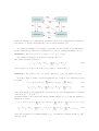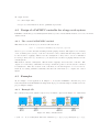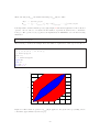
1
PnPMPC Toolbox v. 0.9 - User manual1 Stefano Riverso, Alberto Battocchio, and Giancarlo Ferrari-Trecate Dipartimento di Ingegneria Industriale e dell’Informazione Universit`a degli Studi di Pavia via Ferrata, 1 27100 Pavia Italy March, 2013 1 The research leading to these results has received funding from the European Union Seventh Framework Programme [FP7/2007-2013] under grant agreement n◦ 257462 HYCON2 Network of excellence. Chapter 1 Introduction The PnPMPC toolbox is a GNU-licensed MatLab toolbox for the modeling of constrained Large Scale Systems (LSS) with linear time-invariant dynamics and for the implementation of the Plugand-Play (PnP) Decentralized (De) Model Predictive Control (MPC) schemes described in [1]. The PnPMPC toolbox offers also several functionalities for handling zonotopes set and for computing invariant sets. The realization of the toolbox has received funding from the European Union Seventh Framework Programme [FP7/2007-2013] under grant agreement n◦ 257462 HYCON2 Network of excellence. The last version of the PnPMPC toolbox can be downloaded at the webpage http://sisdin.unipv.it/pnpmpc/pnpmpc.php Please send bug reports, questions or comments to pnpmpc [email protected] 1.1 Notations • R is the set of real number. • N is the set of integers. • a : b is the set of integer {a, a + 1, . . . , b} • A ≥ 0 means that the matrix A is positive semi-definite. A > 0 means that matrix A is positive definite. • A = diag(A11 , . . . , Ass) is the block diagonal matrix A11 0 0 .. . 0 0 0 0 Ass • x[i] , u[i] , y[i] , d[i] , u[ceni ] are column vectors of suitable dimensions. 1 (1.1) • x = (x[1] , x[2] , . . . , x[s] ) means that x is composed by column vectors x[i] , i = 1 : s stacked in a single column, i.e. x[1] x[2] x= (1.2) .. . x[s] • The symbol ⊕ denotes the Minkowski sum, e.g. A = B ⊕ C if and only if A = {a : a = b + c, ∀b ∈ B, ∀c ∈ C}. Ls • i=1 Gi = G1 ⊕ . . . ⊕ Gs . Qs • × indicates the cartesian product and i=1 Gi = G1 × . . . × Gs Definition 1. A polyhedron X is the intersection of a finite number of closed half spaces. Therefore we can represent a polyhedron either as X = {x ∈ Rn : Hx ≤ K} where H ∈ Rv×n and K ∈ Rv (H-representation) or as a convex hull of vertices (V-representation). Definition 2. A zonotope is a centrally symmetric convex polytopes: given a vector p ∈ Rn and a matrix Ξ ∈ Rn×m , the zonotope X ⊆ Rn is the set X = {x | x = p + Ξd, ||d||∞ ≤ 1}, with d ∈ Rm . We will refer to this representation as G-representation. 1.2 Required toolboxes The PnPMPC toolbox requires the following toolboxes to be installed. • Control System Toolbox [2] which implements the class ss (state-space). We also use the function c2d for time-discretization. • MPT toolbox [3] which implements the polytope class. • YALMIP toolbox [4] which include the optimization function solvesdp that is called for solving optimization problems. • GraphViz4MatLab toolbox [5] that allows one to plot the graph of a large-scale system composed by interconnected systems. Please note that MPT, YALMIP and GraphViz4MatLab get automatically installed when installing PnPMPC (with an option to avoid their installation in case you already have them. One can check if all required toolboxes are correctly installed with the following instructions. yalmiptest mpt_init 2 1.3 Installed solvers The following solvers get automatically installed when installing PnPMPC. • Sedumi [6]. • GLPK (GNU Linear Programming Kit) [7]. • SDPT3 [8]. 1.4 Installation of the PnPMPC toolbox • Step 1 Add the folder of the PnPMPC toolbox and its subfolders in the MatLab path. • Step 2 Run pnpmpc toolbox init Remark 1: if you already have installed MPT and/or YALMIP, pnpmpc toolbox init will give the possibility of skipping their installation. However, we guarantee that PnPMPC works correctly only with the versions of MPT and YALMIP supplied with PnPMPC. Therefore, if you want to be 100% sure that everything works, remove any previous copies of MPT and YALMIP from your disk before installing those supplied with PnPMPC. Also remove any MPT and YALMIP directory from your Matlab path. Remark 2: also for the solvers, pnpmpc toolbox init will give the possibility of skipping their installation. However, if you want to be 100% sure that everything works, remove any previous copies of the solvers from your disk before installing those supplied with PnPMPC. Also remove any solver directory from your MatLab path. Remark 3: we tested PnPMPC-toolbox on MatLab R2009b and newer version for Windows, Linux and MacOS. For older versions of MatLab we cannot guarantee that everything works correctly. 1.5 Directories The PnPMPC toolbox consists of the following directories • ./pnpmpc toolbox/@epsilon mRPI contains methods for computing outer-approximation of minimal robust positively invariant sets • ./pnpmpc toolbox/@localControlLyapunov contains methods for computing control invariant sets • ./pnpmpc toolbox/@lss contains methods for modeling of LSS • ./pnpmpc toolbox/@parameterizedRCI contains methods for computing robust control invariant sets • ./pnpmpc toolbox/@pnpmpc contains methods for design of PnPMPC controllers • ./pnpmpc toolbox/@polytope contains functions of MPT toolbox improved to use zonotope sets 3 • ./pnpmpc toolbox/@subss contains methods for the modeling of a subsystem of an LSS • ./pnpmpc toolbox/@zonotope contains methods for using zonotope sets • ./pnpmpc toolbox/@zonotopeRCI contains methods for computing zonotopic robust control invariant sets • ./pnpmpc toolbox/docs contains html documentation • ./pnpmpc toolbox/examples contains examples demonstrating the functionalities of PnPMPC toolbox • ./pnpmpc toolbox/extra contains extra useful functions • ./pnpmpc toolbox/solvers contains solvers provided with PnPMPC toolbox • ./pnpmpc toolbox/toolbox contains additional toolboxes provided with PnPMPC toolbox For familiarizing quickly with PnPMPC toolbox, examples are supplied in the directory ./pnpmpc toolbox/examples. These .m files can also be used as templates for your personal experiments. 4 Chapter 2 Modeling of interconnected systems In this chapter we describe the class of systems considered in the PnPMPC toolbox. Features of subsystems and their interconnections will be discussed in details. The use of the PnPMPC toolbox for modeling purposes will be illustrate in Chapter 3. 2.1 Large-scale linear systems In this toolbox, we consider Multi-Input Multi-Output (MIMO), Linear Time-Invariant (LTI) systems either in discrete or continuous time. An LSS is composed by s physically interconnected subsystems. In the following, dependence of variables from time will be omitted, except where indicated. The dynamics of subsystem i ∈ M = 1 : s is X x+ [i] = Aii x[i] + Bii u[i] + (Aij x[j] + Bij u[j] ) (2.1) j∈Ni where x[i] ∈ Rni is the state at time k, x+ [i] is the state at time k + 1 (for continuous-time systems, dx[i] mi x+ is the local input at time k. [i] stands for dt ) and u[i] ∈ R ni ×ni , Aij ∈ Rni ×nj , Bii ∈ Rni ×mi and Bij ∈ Rni ×mj . Next, we define Moreover we have Aii ∈ R the index set Ni appearing in (2.1). Definition 3. Subsystem i is dynamically coupled to subsystem j if Aij 6= 0. Definition 4. Subsystem i is input coupled to subsystem j if Bij 6= 0. It is possible to use graph theory to represent the coupling between the subsystems. The coupling graph of a system is directed graph where nodes are the subsystems, and the set of edges is given by ξ = {(i, j) : i 6= j, Aij 6= 0 or Bij 6= 0}. An example is given in Figure 2.1. Coupling allows us to define the predecessors of a subsystem. Definition 5. The set of predecessors to subsystem i is Ni = {j : (i, j) ∈ ξ}. 5 Figure 2.1: Example of a coupling graph of a system composed by four subsystems. A black arrow from system i to system j means that Aij 6= 0; a red arrow means Bij 6= 0. For example, from Figure 2.1 one has N2 = {1, 4} since A21 , B21 and A24 are not null matrices. We also define the set of successors of subsystem i, i.e. the set of subsystems influenced by it. Definition 6. The set of successors to system i is Si = {j : (j, i) ∈ ξ}. For example, from Figure 2.1 one has S2 = {4} since A42 6= 0. The output of system i is given by: X y[i] = Cii x[i] + Dii u[i] + (Cij x[j] + Dij u[j] ) (2.2) j∈Ni where y[i] ∈ Rpi , Cii ∈ Rpi ×ni , Dii ∈ Rpi ×mi , Cij ∈ Rpi ×nj and Dij ∈ Rpi ×mj . Definition 7. Two systems i and j are output coupled if Cij or Dij are different from zero. It is also possible to include exogenous signals that act on system i, by replacing (2.1) and (2.2) with: X X x+ [i] = Aii x[i] + Bii u[i] + (Aij x[j] + Bij u[j] ) + Mij d[j] (2.3) y[i] = Cii x[i] + Dii u[i] + j∈Ni j∈Ndi X X (Cij x[j] + Dij u[j] ) + j∈Ni Nij d[j] (2.4) j∈Ndi where d[j] ∈ R is an exogenous signal, Nd,i ⊂ N is the set of exogenous signals that act on system i and Mij ∈ Rni ×1 , Nij ∈ Rpi ×1 . We further enhance our model by introducing centralized inputs ucen,[j] , so that the dynamics of subsystem i becomes: X X X x+ [i] = Aii x[i] + Bii u[i] + (Aij x[j] + Bij u[j] ) + Mij d[j] + Bcen,ij ucen,[j] (2.5) j∈Ni y[i] = Cii x[i] + Dii u[i] + X j∈Nd,i (Cij x[j] + Dij u[j] ) + j∈Ni X j∈Nd,i Nij d[j] + j∈Nu,i X Dcen,ij ucen,[j] (2.6) j∈Nu,i where Nu,i ⊂ N is the set of centralized inputs ucen,[j] , j ∈ R that act on system i and Bcen,ij ∈ Rni and Dcen,ij ∈ Rpi . 6 The difference between u[i] and ucen[i] is that u[i] is a local input, i.e. the output of a local regulator for subsystem i while ucen,[j] is a global input that cannot be computed locally. From models (2.5) and (2.6), the collective dynamics of the resulting LSS is x+ = A + Bu + Md + Bcen ucen (2.7) y = Cx + Du + Nd + Dcen ucen (2.8) x = (x[1] , x[2] , . . . , x[s] ) ∈ Rn (2.9) where: is the overall state and n = P is the overall input and m = is the overall output and p = i∈M P ni , u = (u[1] , u[2] , . . . , u[s] ) ∈ Rm i∈M P (2.10) mi , y = (y[1] , y[2] , . . . , y[s] ) ∈ Rp i∈M (2.11) pi , d ∈ Rnd (2.12) collects the exogenous signals acting on the overall system and ucen ∈ Rnu (2.13) collects the centralized inputs acting on the overall system. Moreover one has: A11 . . . A1s B11 . . . . n×n .. .. A = .. B = .. ∈R As1 . . . Ass Bs1 . . . B1s .. .. n×m . . ∈R . . . Bss (2.14) All other matrices in (2.7) and (2.8) have a similar block structure. Moreover has C ∈ Rp×n , D ∈ Rp×m , M ∈ Rn×nd , N ∈ Rp×nd , Bcen ∈ Rn×nu and Dcen ∈ Rp×nu . The matrix A can also be split into matrices Ad and Ac , defined as: A11 0 0 .. AD = AC = A − AD (2.15) . 0 0 0 0 Ass Apparently AD collects all the local dynamics of the subsystems, while AC collects coupling terms between subsystems. The same decomposition can be done for the matrices B, C, D appearing in (2.7) and (2.8). Each subsystem can be equipped with the following constraints: x[i] ∈ Xi ⊆ Rni (2.16a) mi (2.16b) pi (2.16c) u[i] ∈ Ui ⊆ R y[i] ∈ Yi ⊆ R We furthermore assume that Xi , Ui and Yi are polyhedra. 7 It is also possible to define coupling constraints between two or more subsystems. In the case of two subsystems (i and j) we have (x[i] , x[j] ) ∈ Xij ⊆ Rni +nj (2.17a) mi +mj (2.17b) (y[i] , y[j] ) ∈ Yij ⊆ Rpi +pj (2.17c) (u[i] , u[j] ) ∈ Uij ⊆ R Constraints for the global lss system can be defined as follow x ∈ X ⊆ Rn (2.18a) m (2.18b) y ∈ Y ⊆ Rp (2.18c) u∈U⊆R where X= Y i∈M U= Y i∈M Y= Y i∈M Xi ∩ ( \ Xij ) (2.19a) Uij ) (2.19b) Yij ) (2.19c) i,j∈M,i6=j Ui ∩ ( \ i,j∈M,i6=j Yi ∩ ( \ i,j∈M,i6=j Moreover we can define constraints for the exogenous signals and for the centralized inputs: d ∈ D ⊆ Rnd (2.20a) nu (2.20b) ucen ∈ Ucen ⊆ R Recalling Definition 1 we have matrices Hx , Hu , Hu , Hd , Hcen and vectors Kx , Ku , Ku , Kd , Kcen of suitable dimensions such that X = {x ∈ Rn : Hx x ≤ Kx }. (2.21a) U = {u ∈ Rm : Hu u ≤ Ku }. (2.21b) p Y = {y ∈ R : Hy y ≤ Ky }. D = {d ∈ R nd (2.21c) : Hd d ≤ Kd }. (2.21d) nu (2.21e) Ucen = {ucen ∈ R : Hcen ucen ≤ Kcen }. Moreover, for each subsystem i ∈ M there are matrices Hxi , Hui , Hyi and vectors Kxi , Kui , Kyi such that Xi = {x[i] ∈ Rni : Hxi x[i] ≤ Kxi }. (2.22a) Ui = {u[i] ∈ Rmi : Hui u[i] ≤ Kui }. (2.22b) pi : Hyi y[i] ≤ Kyi }. (2.22c) Dj = {d[j] ∈ R : Hd,j d[j] ≤ Kd,j } (2.23) Yi = {y[i] ∈ R In a similar way, for d[j] , j ∈ 1 : nd we have and for all ucen,[j] , j ∈ 1 : nu it holds Ucenj = {ucen,[j] ∈ Rnuj : Hcen,j ucen,[j] ≤ Kcen,j } Coupling constraints have a totally analogous representation. 8 (2.24) Chapter 3 Modeling of LSS: the lss and subss classes 3.1 The lss class There are many MatLab toolboxes that offer facilities for modeling MIMO, LTI systems. However, most of them have not been designed to handle the interconnection of several subsystems. Therefore it is not immediate to manage an LSS, that means to add/remove subsystems, to extract a subsystem, to set coupling terms, etc. In the PnPMPC toolbox we have implemented methods for these tasks so as to ease the modeling of systems in the form (2.7) and (2.8). Moreover, the system object stores the constraints and some other useful pieces of information. The properties of an lss object are: • numSys: the number s of subsystems composing the LSS; • Ts: the sampling time; • all matrices appearing in (2.7) and (2.8); • ni, mi, pi: vectors of s elements which collect the numbers of states, inputs and outputs of every subsystem as in (2.9), (2.10) and (2.11); • numExo, numICen are respectively nd in (2.12) and nu (2.13); • all constraint matrices H and K appearing in (2.21); • Hdeltau,Kdeltau that will be explained in Section 3.2.4; • coupling, name, that will be explained in Section 3.1; • namex, nameu, namey, named, nameucen in order to assign names to variables (see Section 3.1). Memory optimization Taking into account that usually LSS have a sparse structure and therefore matrices in (2.7) and (2.8) have many zero elements, we decided to use of MatLab sparse matrices by default. This 9 usually allows one to save a considerable amount of memory. To visualize the matrices in the full format, is enough to use the MatLab command full. To save further memory we also used the following trick. If in (2.8) one has y = x then: • the matrix C is the identity matrix of order n • D is a matrix of zeros ∈ Rn×m • there is no exogenous signal or centralized input acting on the output. Therefore, we decided to not save these matrices. However if the user requires them with a get method, they will be generated upon demand. In the following, this particular form of the output equation will be called the standard setting. Model discretization Continuous-time models can be discretized using the method clss2dlss (that means continuous LSS to discrete LSS), with this declaration: dobjlss = objlss.clss2dlss(Ts, method) where Ts is the sampling time and method is the discretization technique. All the discretization techniques of the function c2d of the Control System Toolbox (which converts continuous-time systems to discrete-time models) are implemented, like zoh (zero order hold) or Tustin (see help c2d for more help). The c2d discretization methods are not always a good choice for LSS, because for exact discretization one has to compute the exponential of matrix A. Since A is usually a large matrix with many zero elements, one has that: • computing the exponential is time-consuming, • elements that are zeros in the matrix A of the continuous-time model can be different from zero in the exponential matrix. Therefore, exact discretization creates coupling between subsystems that were originally decoupled. To avoid these problems we also implemented system-by-system discretization. That means that each subsystem in (2.5) and (2.6) is discretized considering states x[j] , j 6= i as exogenous inputs. We can save computational time because we discretize sequentially subsystems that usually have low dimension and we do not create new couplings among subsystems. For using this technique, set ’subsystem’ as method. Other utilities There are some other object’s properties that we have not explained yet. • coupling is a matrix with size numSys×numSys composed by Boolean elements: element (i, j) is 1 only if subsystem i is dynamically coupled or input coupled to subsystem j, i.e. (i, j) ∈ ξ. • name is a cell array of strings with size 1 × numSys, that associates a name to every subsystem in the lss object. It is possible to set name when calling the addSystem method. 10 If a name is not supplied to addSystem, a default name will be chosen and a warning appears. Every method that needs a subsystem as input, has been designed to use these names as an alternative to subsystem numbers. However, it is better to use numbers when possible, because MatLab is slower when working with strings. • namex, nameu, namey, named, nameucen are cell arrays of strings, each with dimension 1 × numSys. The element in position i stores information related to i-th subsystem. For example namex(1,i) is a matrix of strings of ni rows which stores the name associated to every state of i-th subsystem. Similar remarks can be applied to properties nameu, namey, named, nameucen that are related to system input, output, exogenous signals and centralized input. Names can be written with the LATEXsyntax and are also used in plots of subsystems or time-evolution of individual variables. 3.2 How to use the lss class through examples In the following sections, we provide several examples with comments that illustrate the modeling process with the PnPMPC toolbox. Section titles corresponds to m-files that can be found in the ./examples/lss directory. 3.2.1 example1lss.m We show how to model the two coupled mass-spring-damper systems represented in Figure 3.1. The model is Figure 3.1: System modeled in example1lss.m " # " # " # x˙ [1] x[1] u =A + B [1] x˙ [2] x[2] u[2] (3.1) where x[1] is composed by x[1,1] , the displacement of first mass with respect to a given equilibrium position, and x[1,2] , the velocity of the first mass. Similarly x[2] is composed by x[2,1] and x[2,2] . Moreover u[1] and u[2] are forces applied to the first and second mass, respectively. We also have # " # # " " 0 0 0 1 A11 A12 , A12 = A21 = k (3.2) , A11 = A22 = A= h h k −M A21 A22 −M M M B = diag(B11 , B22 ), B11 = B22 = First of all we present the methods that will be used. 11 " 0 100 M # (3.3) The lss method lss is the constructor of the homonymous class, with this declarations objlss=lss(A,B,ni,mi,C,D,pi,name,Ts) where - A and B are the matrices in (2.7); - ni and mi are vectors storing the sizes of blocks Aij and Bij in matrices A and B; - C and D are the matrices in (2.8); - pi is a vector storing the sizes of blocks Cij and Dij in matrices C and D; - name is an optional string defining the system name; - Ts is the sampling time, that can be: – Ts = [ ] for continuous-time system; – Ts > 0 for discretized system with sampling time Ts; – Ts = -1 for system already in the discrete-time form. It is possible to introduce directly the matrices of the collective system system (2.7) and (2.8) but this operation is usually time consuming and error-prone. Hence in the example we will start from an empty object and add subsystems with addSystem method. The addSystem method The addSystem method adds to an lss object a single subsystem. The method declaration is objlss = objlss.addSystem(Ai,Bi,Ci,Di,name,Ts) where the subsystem matrices are Ai, Bi, Ci, Di as defined in (2.5) and (2.6). The arguments name and Ts have the same meaning as in the lss class. We also highlight that addSystem could also receive one input argument only: it can be a subss object (see Section 3.3) or a ss object (state-space object of System Control Toolbox) or a tf object (transfer function object of System Control Toolbox). The addCoupling method By using addSystem method only the block diagonal part of the matrices A, B, C and D in (2.7) and (2.8) can be set. If system i is coupled to system j, one or more blocks among Aij , Bij , Cij or Dij are non zero. The method addCoupling allows one to set them. The method declaration is objlss = objlss.addCoupling(i,j,Aij,Bij,Cij,Dij) where: i and j represent indexes of the the coupled subsystems. It is possible to use subsystem names instead of numbers i and j. Code for modeling system (3.1) With the three methods presented above it is possible create the model of coupled masses. 12 M = 5; % mass k = 0.5; % elastic constant of the springs h = 5; % damping coefficient % creation of an empty lss object modelCart = lss ; A = [ 0 , 1; -k / M , -h / M ]; B =[ 0; 100/ M ]; % system 1 modelCart = modelCart . addSystem (A , B ); % system 2 modelCart = modelCart . addSystem (A , B ); % coupling among subsystems 1 and 2 Aij = [ 0 , 0 ; k / M , h / M ]; modelCart = modelCart . addCoupling (1 ,2 , Aij ); modelCart = modelCart . addCoupling (2 ,1 , Aij ); % plot graph of subsystems modelCart . plot In general, the declaration of the methods contains many optimal parameters, that are optional and the user can provide only meaningful quantity. In the example above, parameters Ci,Di,name,Ts are not supplied to addSystem method, because we are assuming y = x, so we are in the “standard setting” discussed in Section 3.1. Moreover, we do not want to associate a name to the model and we are defining a model in continuous time, so that Ts is empty. Similar remarks apply to all methods of the toolbox. 3.2.2 example2lss.m Now we will add an exogenous signal and a centralized input to the lss object modelCart through example1lss.m. With reference to (2.7) and (2.8), we want to set 0 1 M= 16 2 0 0 , 0 3 0 0 N= 0 0 0 0 , 0 Bcen 0 0 4 = , 0 5 Like in the previous section, we start with the description of the relevant methods. The addExoInput method The addExoInput method is used to set matrices M and N. The method declaration is objlss = objlss.addExoInput(M,N,i,j) 13 (3.4) and it can be used in two ways: • objlss = objlss.addExoInput(M,N), in this case we set the global M ∈ Rn×nd and N ∈ Rp×nd matrices of the LSS, according to (2.7) and (2.8). • objlss = objlss.addExoInput(M,N,i,j), in this case we set only blocks Mij and Nij of matrices M and N (2.5) and (2.6), i.e. the relation among subsystem i and the exogenous signal j, defined (2.5) and (2.6). The relation among all the other subsystems different from i and exogenous signal j is automatically set as zero if not already defined. The addCentralizedInput method The addCentralizedInput method is used to set matrices Bcen and Dcen . The method declaration is: objlss = objlss.addCentralizedInput(Bcen,Dcen,i,j) and it can be used in two ways: • objlss = objlss.addCentralizedInput(Bcen,Dcen), in this case we set the global Bcen ∈ Rn×nu and Dcen ∈ Rp×nu matrices of the LSS, according to (2.7) and (2.8). • objlss = objlss.addCentralizedInput(Bcen,Dcen,i,j), in this case we set Bcenij and Dcenij of matrices Bcen and Dcen (2.5) and (2.6), i.e. the relation among subsystem i and the centralized input j, defined (2.5) and (2.6). The relation among all the other subsystems different from i and centralized input j is automatically set as zero if not already defined. example1lss ; % specify how exogenous input number 1 affects system 1 ( creation of M ) modelCart = modelCart . addExoInput ([0;1] ,[] , 1 ,1); % specify how exogenous input number 1 affects system 2 ( creation of M ) modelCart = modelCart . addExoInput ([16;2] ,[] ,2 ,1); % specify how exogenous input number 2 affects system 2 ( creation of M ) modelCart = modelCart . addExoInput ([0;3] ,[] ,2 ,2); % instead of calling addExoInput three times we can use % modelCart = modelCart . addExoInput ([0 0; 1 0; 16 0; 2 3] ,[]); % specify how centralized input number 1 affects system 1 ( creation of Bcen ) modelCart = modelCart . addCentral i ze d In p ut ([0;4] ,[] ,1 ,1); % specify how centralized input number 1 affects system 2 ( creation of Bcen ) modelCart = modelCart . addCentral i ze d In p ut ([0;5] ,[] ,2 ,1); % instead of the previous calls to addCentral i ze d In p ut we can use % modelCart = modelCart . addCentral i ze d In p ut ([0;4;0;5] ,[]); 14 % plot all signals modelCart . plot ([] , ' all ') If, like in this case, the user does not need to set the N or Dcen matrix, it is possible to use empty matrices. Empty or not passed parameters are given default values. The same remark applies to all other methods in the toolbox. 3.2.3 example3lss.m This example shows how to exploit modularity in the subsystem interconnection for quickly creating an LSS. The code below allows one to create a string of N mass-spring-damper systems (as shown in Figure 3.2) with different M (mass), different k (elastic constant of the springs) and different h (damping coefficient), verifying the bounds minM ≤ M ≤ maxM , mink ≤ k ≤ maxk and minh ≤ h ≤ maxh. The system is characterized by the matrices: Figure 3.2: Large-scale system to model in example3lss. A11 = " 0 1 k(1) − M(1) h(1) − M(1) # , AN N = " 0 1 −1) − k(N M(N ) −1) − h(N M(N ) ∀i = 2 : N − 1 # " # " 0 0 1 , Bii = 100 Aii = − h(i−1)+h(i) − k(i−1)+k(i) M(i) M(i) M(i) " # " 0 0 0 A(i−1),i = , Ai,(i−1) = k(i−1) h(i−1) k(i−1) − M(i−1) − M(i−1) − M(i) h i Cii = 1 0 , Dii = 0; The MatLab code for the model creation is when N = 1000 is N minM maxM mink maxk minh maxh = = = = = = = 1000; 1; 10; 0.1; 0.9; 0.1; 10; M = minM + rand (1 , N )*( maxM - minM ); 15 # (3.5) 0 − h(i−1) M(i) # k = mink + rand (1 , N -1)*( maxk - mink ); h = minh + rand (1 , N -1)*( maxh - minh ); modelCart = lss ; modelCart = modelCart . addSystem ([0 ,1; - k (1)/ M (1) , - h (1)/ M (1)] ,[0;100/ M (1)] ,... [1 0] ,0); for i =2: N -1 modelCart = modelCart . addSystem ([0 ,1; -( k (i -1)+ k ( i ))/ M ( i ) ,... -( h (i -1)+ h ( i ))/ M ( i )] ,[0;100/ M ( i )] ,[1 0] ,0); modelCart = modelCart . addCoupling (i -1 , i ,[0 ,0; k (i -1)/ M (i -1) ,... h (i -1)/ M (i -1)] , zeros (2 ,1)); modelCart = modelCart . addCoupling (i ,i -1 ,[0 ,0; k (i -1)/ M ( i ) , h (i -1)/ M ( i )] ,... zeros (2 ,1)); end modelCart = modelCart . addSystem ([0 ,1; - k (N -1)/ M ( N ) , - h (N -1)/ M ( N )] ,... [0;100/ M ( N )] ,[1 0] ,0); modelCart = modelCart . addCoupling (N ,N -1 ,[0 ,0; k (N -1)/ M ( N ) , h (N -1)/ M ( N )] ,... zeros (2 ,1)); modelCart = modelCart . addCoupling (N -1 , N ,[0 ,0; k (N -1)/ M (N -1) , h (N -1)/ M (N -1)] ,... zeros (2 ,1)); 3.2.4 example4lss.m This example shows how to add state and input constraints to an lss model. The addition of constraints on output, exogenous signal and centralized input can be done in a similar way. Relevant methods are described next. Methods for adding constraints The addStateConstraint method sets the matrices Hxi and Kxi in (2.22). The method declaration is: objlss = objlss.addStateConstraint (sysindex,H,K) Where sysindex is the number or name of the subsystem to which constraints have to be added and H and K are the matrices Hxi and Kxi in (2.22). It is also possible to create constraints between two or more subsystems, in this case sysindex is a vector of scalars, or a cell array of names of the subsystems involved. Methods that allow one to add constraints to inputs, outputs, exogenous signals and centralized inputs. - objlss = objlss.addInputConstraint(sysindex,H,K) - objlss = objlss.addOutConstraint(sysindex,H,K). Note that if the user tries to insert a constraint on the output, but the system is in standard setting (y = x), the constraint will be converted in a state constraint and a warning will be displayed. - objlss = objlss.addExoConstraint(exoindex,H,K) - objlss = objlss.addCentralizedInputConstraint(ceninputindex,H,K) 16 and works exactly as addStateConstraint. The “double” methods The double methods return matrices H and K related to constraints. The name “double” has been used for coherency with the MPT toolbox [3]. The method declaration is: [Hx,Kx] = objlss.doubleStateConstraint(index,selection) and it returns Hx and Kx matrix related to the states of the subsystem/subsystems expressed in index. index can be a scalar or a string, but also a vector of scalars or a cell array of names, if one is interested in coupling constraints. selection is a Boolean flag with the following meaning - 0: exclusive (default). The state constraints only of the subsystem/subsystems indicated in index will be returned - 1: all. All state constraints which includes the subsystem/subsystems indicated in index will be returned. For example, let c1 be a constraint related to subsystem 1, c3 be a constraint related to subsystem 3 and c13 be a coupling constraint between subsystem 1 and 3. If index = 3 and selection=0 (or not passed) H and K contain only c3 because this is the only constraint that involves subsystem 3 only. If selection = 1, H and K will contain c3 and c13 , i.e. all constraints involving subsystem number 3. Another possible use of this method is: X = objlss.doubleStateConstraint(index,selection) with only one output argument. In this case, X is the polytope (i.e. an object of polytope class, see the documentation of the MPT toolbox for help) of system specified in index giving rise to a state constraint. Also if index contains more than one index, a polytope object will be returned. Other double methods with similar meaning and use are - [Hu,Ku] = objlss.doubleInputConstraint(index,selection) - [Hy,Ky] = objlss.doubleOutConstraint(index,selection) - [Hd,Kd] = objlss.doubleExoConstraint(index,selection) - [Hcen,Kcen]= objlss.doubleCenInputConstraint(index,selection) Next, we provide the code for adding constraints (described in the code comments) to the modelCart object. example2lss ; % 0( x_3 )+1( x_4 ) ≤ 3 modelCart = modelCart . addStateCo ns t ra i nt (2 ,[0 ,1] ,3); % 2( x_3 )+1( x_4 ) ≤ 0 and 1( x_3 )+3( x_4 ) ≤ 5 modelCart = modelCart . addStateCo ns t ra i nt (2 ,[2 ,1;1 ,3] ,[0;5]); 17 % 0( x_1 )+1( x_2 )+1( x_3 )+2( x_4 ) ≤ 0 & 3( x_1 )+2( x_2 )+0( x_3 )+1( x_4 ) ≤ 5 modelCart = modelCart . addStateCo ns t ra i nt ([1 ,2] ,[0 ,1 ,1 ,2;3 ,2 ,0 ,1] ,[0;5]); % 2( u_2 ) ≤ 3 modelCart = modelCart . addInputCo ns t ra i nt (2 ,2 ,3); % 1( u_1 )+2( u_2 ) ≤ 3 modelCart = modelCart . addInputCo ns t ra i nt ([1 ,2] ,[1 ,2] ,3); [ Hx Kx ] = modelCart . doubleStat e C on s tr a i nt (1) disp ( ' Hx and Kx are empty because there is no constraint affecting system 1 only ') [ Hu Ku ] = modelCart . doubleInpu t C on s tr a i nt (2 ,1) disp ( ' Hu and Ku contain 2( u_2 ) ≤ 3 and 1( u_1 ) + 2( u_2 ) ≤ 3 because selection is 1 and we consider all the constraints related to system 2 ') Input increment In many systems, rather than constraining the input, it is preferable to bound the input increments δu[i] = u[i] (k + 1) − u[i] (k). With addDeltaUConstraint is possible to define matrices Hδui and Kδui giving rise to the constraints {Hδui δu[i] ≤ Kδui }. The method declaration is objlss = objlss.addDeltaUConstraint (sysindex,Hdeltau,Kdeltau) And the corresponding “double” method is [Hdeltau,Kdeltau] = objlss.doubleDeltaUConstraint(index,selection) 3.2.5 example5lss.m All the methods described above are useful to add subsystems, couplings and constraints to an lss object. But if the user inserts wrong parameters it can be useful to remove system features in a selective way. This is the goal of the methods discussed next. The removeCoupling method objlss = objlss.removeCoupling(i,j,how) This method allows one to remove coupling between subsystems i and j. The variable how can be 'a' or 'b' or 'c' or 'd' and specifies if we want to remove coupling terms in the matrices A, B, C, D, respectively. If how is not passed blocks (i, j) in all matrices A, B, C, D will be removed. See help removeCoupling for more information. The removeExoSignal method objlss = objlss.removeExoSignal(i) This method allows one to remove the exogenous signal d[i] . It deletes the column i of matrices M and N and also the constraints related to this exogenous signals (if present). Note that a coupling 18 constraint related to exogenous signals i and j, after the removal of the signal i becomes a local constraint of signal j. For example, let d[1] + 2d[2] ≤ 10 be a constraint among exogenous signals d[1] and d[2] ; the execution of objlss = objlss.removeExoSignal(1) removes d[1] in the constraint, i.e. the new constraint is 2d[2] ≤ 10. If one wants to remove all constraints where signal d[i] appears, the removeConstraint method can be used. The removeCentralizedInput method objlss = objlss.removeCentralizedInput(i) This method allows one to deletes the centralized input number i. It eliminates the column i of matrices Bcen and Dcen and also the constraints related to this centralized input (if present). Note that a coupling constraint related to centralized inputs i and j , after the removal of i becomes a local constraint of j. If one wants to remove all constraints where centralized input ucen,[i] appears, the removeConstraint method can be used. The removeConstraint method objlss = objlss.removeConstraint(index,flag) This method allows one to remove constraints. index can be, as usually, the subsystem number or name, if we want to remove local constraints. But it can also be a vector of scalars or a cell array of names, if we want to remove coupling constraints. flag can be 'state' or 'in' or 'out' or 'exo' or 'cen' or ’deltau'. In this way it is possible to remove, for instance, state constraints only. If flag is 'exo' or 'cen' we refer to the constraints to exogenous signals d[i] or centralized input, and in this case we have to specify the number of signal/signals interested. If flag is not specified all constraints on states, inputs and outputs of the system in index will be removed. Fore example if flag is empty and index is 1, then X1 , U1 and Y1 will be removed. See help removeConstraint for more information. The removeSystem method objlss=objlss.removeSystem(i) This method allows one to remove the subsystem number i from an lss object. Note that if subsystem i is removed, this triggers the following changes. • if an exogenous signal acts only on subsystem i the method removeExoSignal will be automatically called for removing the signal from the lss model and a warning appears on the screen. The same remark applies to centralized inputs. • if two subsystems i and j are involved in a coupling constraint, and i system is removed, the constraint becomes a local constraint of j. For example, let u[1] + u[2] ≤ 20 be a constraint among subsystems 1 and 2; the execution of objlss = objlss.removeSystem(1) removes u[1] in the constraint, i.e. the new constraint is u[2] ≤ 20. In this example we illustrate the use of the removal methods. We start from the model created in example4lss. 19 example4lss ; % remove exogenous signal number 2 modelCart = modelCart . removeExoSig n al (2); % remove centralized input number 1 modelCart = modelCart . r e m o v e C e n t r a l i z e d I n p u t (1); % remove coupling constraint on the state of system 1 and 2 modelCart = modelCart . removeConst ra i nt ([1 ,2] , ' state ' ); % remove dynamic coupling between 1 and 2 so A12 = zeros modelCart = modelCart . removeCoupli ng (1 ,2 , 'a ' ); % remove subsystem number 2 modelCart = modelCart . removeSystem (2); 3.2.6 Performances of the methods dedicated to modeling We discuss here performances, in terms of memory occupation and execution time of the methods of the PnPMPC toolbox dedicated to modeling. As a first case study, we use the string of N masses described in example1lss.m and example3lss.m with local constraints on states and inputs. In the left panel of Figure 3.3 one can see • the execution time for creating the lss object (blue line), • the execution time for discretizing the lss object using the system-by-system approach (red line) as a function of the number of masses. In the right panel of Figure 3.3 it is reported • the memory occupation (in Kb) due to the continuous-time model (blue line), • the memory occupation (in Kb) due to the discretized model (red line) as a function of the number of masses. These graphics have been obtained on a processor Intel Core i3 3.06 GHz, with 4GB of Ram 1.33 GHz running MatLab r2011a. 3.3 The subss class This class allows one to model individual subsystems and it is useful for: 1. creating a subss object and pass it to an lss object with the addSystem method. In this way, dynamics and constraints of the subsystem will be added to the LSS. 2. extracting a subsystem from an lss object through the getSystem method. 20 Figure 3.3: Performance of PnPMPC toolbox. Many methods of this class have the same name of methods of the lss class and work in the same way. In addition, many properties are the same as those of the lss class. Next we describe only the new ones referring the reader to the html documentation in the doc directory for a comprehensive description of all methods and properties. If we extract subsystem i from an lss object we lose coupling with other subsystems. Therefore we created the following properties to save • couplingA,couplingB,couplingC,couplingD are scalar vectors containing the indices of the subsystems in Ni that are coupled with the extracted subsystem (i.e. subsystem i). couplingA will contain the indices of the subsystems coupled through the A matrix. couplingB, couplingC and couplingD have a similar meaning. • Aij, Bij, Cij, Dij. Aij contains blocks Aij where i is the number of the extracted subsystem and j ∈ couplingA. Same remarks apply to the other properties. 3.3.1 example1subss.m In this example we show how to add a subsystem to an lss object using a subss object. example2lss ; A = [0 ,1; - k /M , - h / M ]; 21 B = [0;100/ M ]; sub = subss (A , B ); sub = sub . addStateCo ns t ra i nt ([3 ,5;0 ,1] ,[1;2]); modelCart = modelCart . addSystem ( sub ); 3.3.2 example2subss After running example3lss, we can extract subsystem 237 as follows. example3lss ; sub = modelCart . getSystem (237) With the previous command, the subsystem sub is an object of the class subss. In this case only local constraints are saved. For example constraints among subsystem 237 and 238 will not be saved. sub will have only the couplingA and Aij matrix, because the subsystem is dynamically coupled with 236 and 238, so sub.couplingA = [236 238] sub.Aij =[A237,236 ; A237,238 ] where A237,236 is the dynamic coupling among subsystems 237 and 236, and A237,238 is the dynamic coupling among subsystems 237 and 238. 22 Chapter 4 The pnpmpc class 4.1 Introduction In this chapter, we introduce the pnpmpc class in order to design a PnPMPC controller for a single subsystem. PnPMPC controllers are described in [1]. In [1], the authors propose a PnP design procedure hinging on the notion of tube MPC [9] for handling coupling among subsystems, and aim at stabilizing the origin of the whole closedloop system while guaranteeing satisfaction of constraints on local inputs and states. The model of subsystem i, i ∈ M is given by (2.3) and (2.4) and we consider that each subsystem i is input decoupled, i.e. Bij = 0, i 6= j. Our control design procedure will hinge on the following assumptions. Assumption 1. The matrix pairs (Aii , Bi ) ∀i ∈ M are controllable. Assumption 2. Constraints Xi and Ui , i ∈ M are compact and convex polytopes containing the origin in their nonempty interior. L Let Zi be an RCI1 set for the nominal2 subsystem i where the coupling term j∈Ni Aij Xj is treated as a disturbance. We design the following controller for subsystem i C[i] : u[i] = v[i] + κ ¯ i (x[i] − x ¯[i] ) (4.1) where κ ¯i : Zi → Ui is any feedback control law guaranteeing x[i] ∈ Zi ⇒ x+ [i] ∈ Zi , ∀x[j] ∈ Xj , j ∈ Ni . Following [9], we set in (4.1) v[i] (t) = v[i] (0|t), (4.2) x ¯[i] (t) = x ˆ[i] (0|t) where v[i] (0|t) and xˆ[i] (0|t) are optimal values of the variables v[i] (0) and xˆ[i] (0), respectively, 1 Robust Control Invariant (RCI) set Consider the discrete-time Linear Time-Invariant (LTI) system x(t + 1) = Ax(t) + Bu(t) + w(t), with x(t) ∈ Rn , u(t) ∈ Rm , w(t) ∈ Wn and subject to constraints u(t) ∈ U ⊆ Rm and w(t) ∈ W ⊂ Rn . The set X ⊆ Rn is an RCI set with respect to w(t) ∈ W, if ∀x(t) ∈ X then there exist u(t) ∈ U such that x(t + 1) ∈ X, ∀w(t) ∈ W. 2 Model of subsystem i without coupling terms. 23 appearing in the MPC-i problem PN i (x[i] (t)) = min N i −1 X v[i] (0:Ni −1) k=0 x ˆ[i] (0) x[i] (Ni )) ℓi (ˆ x[i] (k), v[i] (k)) + Vfi (ˆ x[i] (t) − xˆ[i] (0) ∈ Zi (4.3a) (4.3b) x ˆ[i] (k + 1) = Aii x ˆ[i] (k) + Bi v[i] (k), ˆ x ˆ[i] (k) ∈ Xi , k ∈ 0 : Ni − 1 (4.3c) k ∈ 0 : Ni − 1 (4.3d) v[i] (k) ∈ Vi , ˆf x ˆ[i] (Ni ) ∈ X k ∈ 0 : Ni − 1 (4.3e) (4.3f) i In (4.3), Ni ∈ N is the control horizon, ℓi : Rni ×mi → R+ is the stage cost, Vfi : Rni → R+ is the ˆ f is the terminal set. Moreover, from (5.3c) and (5.3e), the tightened constraints final cost and X i ˆ i and Vi are defined respectively as X ˆ i = Xi ⊖ Zi , X Vi = Ui ⊖ κ ¯ i (Zi ). (4.4) Therefore, in order to design a PnPMPC controller for subsystem i we need to solve the following problem. Problem Pi : Compute nonempty RCI Zi for the nominal subsystem i treating the coupling ˆ i and Vi term as a disturbance. Compute sets X We highlight that Problem Pi can be solved using efficient procedure proposed in [10] that ˆ i and Vi can be computed using requires the solution of a suitable LP problem. Moreover X optimizers from the LP problem. If Problem Pi cannot be solved, we declare that it is impossible to design a PnPMPC controller for subsystem i. The interested reader is refer to [1]. 4.1.1 The pnpmpc method Assume subss stores the model of subsystem i given by (2.3) and (2.4). Controller C[i] is created through objpnpmpc = pnpmpc (subss,N,Xj,k,options) where N is the receding horizon, Xj is a cell array {Hxj , Kxj } such that neighbors states x[j] , j ∈ Ni are in the set Xj = {xj|Hxj xj ≤ Kxj }. k is a parameter of Algorithm 1 in [1] and must be ≥ of the controllability index of the pair (Aii , Bi ). One can also set a cell array {kmin,kmax} in order to try different k. options is used to set the sdpsettings for yalmip (see yalmip manual for details [4]). We propose two methods to compute the terminal region and the terminal penalty. 4.1.2 The XFqpmax method Using XFqpmax we compute a quadratic terminal region using procedures proposed in [11]. In particular we consider ref ref ′ ′ ℓi (ˆ x[i] (k), v[i] (k)) = (ˆ x[i] (k)− x ˆref x[i] (k)− x ˆref [i] (k)) Q(ˆ [i] (k))+(v[i] (k)−v[i] (k))) R(v[i] (k)−v[i] (k))) 24 ′ x[i] (Ni )) = (ˆ x[i] (Ni ) − xˆref x[i] (Ni ) − xˆref Vfi (ˆ [i] (Ni )) S(ˆ [i] (Ni )) ˆ fi = {β ∈ Rni : β ′ Sβ ≤ 1} X where Q = Q′ ≥ 0 ∈ Rni ×ni , R = R′ > 0 ∈ Rmi ×mi and S = S ′ ≥ 0 ∈ Rni ×ni . xˆref [i] (k) and ref v[i] (k) are the state and input reference trajectories for tracking capabilities. We can design the terminal penalty S and the ellipsoidal terminal constraint executing the function objpnpmpc = objpnpmpc.XFqpmax(Q,R,options) 4.1.3 The zeroTerminal method Using zeroTerminal we compute a zero terminal constraint as proposed in Chapter 2 in [12]. In particular we consider ref ref ′ ′ ℓi (ˆ x[i] (k), v[i] (k)) = (ˆ x[i] (k)− x ˆref x[i] (k)− x ˆref [i] (k)) Q(ˆ [i] (k))+(v[i] (k)−v[i] (k))) R(v[i] (k)−v[i] (k))) x[i] (Ni )) = 0 Vfi (ˆ ˆ fi = xˆref (Ni ) X [i] ref where Q = Q′ ≥ 0 ∈ Rni ×ni and R = R′ > 0 ∈ Rmi ×mi . xˆref [i] (k) and v[i] (k) are the state and input reference trajectories for tracking capabilities. We can design the terminal penalt and the ellipsoidal terminal constraint executing the function objpnpmpc = objpnpmpc.zeroTerminal(Q,R) 4.1.4 The uRH method In order to compute the constrol action u[i] we need to solve the optimization problem (4.3). The control action is computed executing the function [ u diagnostics ] = objpnpmpc.uRH(x0,din,xcrefin,vrefin,options) • x0 is the initial state x[i] (0), a vector of dimension ni × 1 for a decentralized implementation of PnPMPC controllers. For a distributed implementation (as in Section 5 of [1]), we consider x0 as a cell array x[i] (0), x[j] (0) where x[i] (0) is the initial state for the current subsystem and x[j] (0) is the state of predecessor subsystems. • xcrefin means the reference state of nominal system (ˆ xref ) over the control horizon; it can be expressed as a vector (ni × 1, if reference is constant over the control horizon) or a matrix (ni × N , the columns 1 refer to the values at the time instant 1 within the control horizon, columns 2 refer to the values at time 2, etc.). If this parameter is empty or not passed it is setted to zero by default. • vrefinin means the reference input of nominal system (vref ) over the control horizon; it can be expressed as a vector (mi × 1, if reference is constant over the control horizon) or a matrix (mi × N , the columns 1 refer to the values at the time instant 1 within the control horizon, columns 2 refer to the values at time 2, etc.). If this parameter is empty or not passed it is setted to zero by default. • options sdpsettings object for yalmip options. 25 As output we have: • u control input value; • diagnostics information about the optimization problems. 4.2 Design of a PnPMPC controller for a large-scale system PnPMPC controllers C[i] for each subsystem in an lss object are created with the method createCtrlPnPMPC described next. 4.2.1 The createCtrlPnPMPC method This method acts on an lss object, and it is called as follows: ctrl = createCtrlPnPMPC(objlss,N,k,option) where N,options have the same meaning as in the pnpmpc method. The input k is a cell array of two elements {kmin,kmax}: both kmin and kmax can be scalars and then they will be used for all execution of pnpmpc function for the i-subsystem or they can be vectors of dimension 1×numSys, where kmin(i) and kmax(i) are used for the execution of pnpmpc function for the i-th subsystem. This method extracts a subsystem, calls the method pnpmpc and creates the controller. The output ctrl is an array of dimension 1×numSys and in the position i it is stored the controller for subsystem i. After the creation of the controllers, we can run XFqpmax or zeroTerminal methods, for setting terminal constraints, and then the uRH method, to compute the control inputs. 4.3 Examples As an example of real application, in Chapter 5, we describe PnPMPC controllers for power network systems and run simulations using methods proposed in this chapter. In this section we propose simpler example. 4.3.1 Example 1D We consider a large-scale system composed by N masses coupled as in Figure 4.1. Each mass Figure 4.1: Array of masses in 1D. i ∈ M = 1 : N , is a subsystem with state variables x[i] = (x[i,1] , x[i,2] ) and input u[i] = u[i,1] , 26 where x[i,1] is the displacements of mass i with respect to a given equilibrium position, x[i,2] is the horizontal velocity of the mass i and 100u[i,1] is the force applied to mass i in the horizontal direction. The values of mi have been extracted randomly in the interval [5, 10] while spring constants and damping coefficients are identical and equal to 0.5. Subsystems are equipped with the state constraints ||x[i,1] ||∞ ≤ 1.5, ||x[i,2] ||∞ ≤ 0.8, i ∈ M and with the input constraints |u[i] | ≤ βi , where βi have been randomly chosen in the interval [1, 1.5]. We obtain models Σ[i] by discretizing continuous-time models with 0.2 sec sampling time, using zero-order hold discretization for the local dynamics and treating x[j] , j ∈ Ni as exogenous signals. At all time steps t, the control action u[i] (t) computed by the controller Ci , for all i ∈ M, is kept constant during the sampling interval and applied to the continuous-time system. In order to create the large-scale system composed by N masses, we can use the function makeModelTrucks1D as follows N = 4; [ modelTrucks 1D c modelTrucks1D d ] = makeModelTr u ck s 1D ( N ); where N is the number of trucks, modelTrucks1Dc and modelTrucks1Dd are the lss objects of the continuous-time and discrete-time models, respectively in form of lss objects. We can design local controllers executing the function options = sdpsettings ( ' verbose ' ,0); Trucks1Dpnp = makePnpmpcT ru c ks 1 D ( modelTrucks1Dd , options ); whose instructions are described next. The Controllers, C[i] , i ∈ M are generated a follows. Trucks1Dpnp is an array of N pnpmpc objects. NMPC = 20; % prediction horizon options = sdpsettings ( ' verbose ' ,0); Trucks1Dpnp = modelTrucks1 D d . createCtrlPn PM P C ( NMPC ,{1 ,30} , options ); Then we add a zero terminal constraint to each controller using the following instructions. Q = 10* eye (2); R = 1; parfor i =1: modelTrucks1 Dd . numSys Trucks1Dpnp ( i ) = Trucks1Dpnp ( i ). zeroTerminal (Q , R ); end We note that the functions makePnpmpcTrucks1D or modelTrucks1Dd.createCtrlPnPMPC could take some minutes to be completely executed if N is large. If you want take less time for the execution, we recommend to install CPLEX optimizer [13] that is free available for academic use. To start a simulation, we can use the function runSimTrucks1D in the following way options = sdpsettings ( ' verbose ' ,0 , ' solver ' , ' sdpt3 ' ); x0 = repmat ([1 0] ' , N ,1); 27 Tsim = 20; [ x u ] = runSimTrucks 1D ( Tsim , x0 , modelTrucks1Dc , modelTrucks1Dd , Trucks1Dpnp , options ); This function computes the control action using the method uRH of the pnpmpc class. We used sdpt3 solver, that is installed with the toolbox, but we really recommend the use of CPLEX. 4.3.2 Example 2D We consider a large-scale system composed by N masses coupled as in Figure 4.3.2 (for the case of N = 1024) where the four edges connected to a point correspond to springs and dampers arranged as in Figure 4.2. Hereafter we assume that N = 2z for some z ∈ N, z > 0. Each ... mj1 hi,j1 ki,j1 ki,j4 ... ki,j2 mi mj4 mj2 hi,j4 ... hi,j2 hi,j3 ki,j3 mj3 ... Figure 4.2: Array of masses: details of interconnections. mass i ∈ M = 1 : N , is a subsystem with state variables x[i] = (x[i,1] , x[i,2] , x[i,3] , x[i,4] ) and input u[i] = (u[i,1] , u[i,2] ), where x[i,1] and x[i,3] are the displacements of mass i with respect to a given equilibrium position on the plane (equilibria lie on a regular grid), x[i,2] and x[i,4] are the horizontal and vertical velocity of the mass i, respectively, and 100u[i,1] (respectively 100u[i,2]) is the force applied to mass i in the horizontal (respectively, vertical) direction. The values of mi have been extracted randomly in the interval [5, 10] while spring constants and damping coefficients are identical and equal to 0.5. Subsystems are equipped with the state constraints ||x[i,j] ||∞ ≤ 1.5, j = 1, 3, ||x[i,l] ||∞ ≤ 0.8, i ∈ M, l = 2, 4 and with the input constraints ||u[i] ||∞ ≤ βi , where βi have been randomly chosen in the interval [1, 1.5]. We obtain models Σ[i] by discretizing continuous-time models with 0.2 sec sampling time, using zero-order hold discretization for the local dynamics and treating x[j] , j ∈ Ni as exogenous signals. At all time steps t, the control action u[i] (t) computed by the controller Ci , for all i ∈ M, is kept constant during the sampling interval and applied to the continuous-time system. 28 50 Time: 6.0 40 30 20 10 0 −10 −20 −30 −40 −40 −30 −20 −10 0 10 20 30 40 50 Figure 4.3: Position of the N = 1024 trucks on the plane. In order to create the large-scale system composed by N masses, we can use the function makeModelTrucks2D as follows N = 4; [ modelTrucks 2D c modelTrucks2D d ] = makeModelTr u ck s 2D ( N ); where N is the number of trucks, modelTrucks2Dc and modelTrucks2Dd are the continuoustime and discrete-time large-scale models, respectively in form of lss objectes. We can design local controllers executing the function options = sdpsettings ( ' verbose ' ,0); Trucks2Dpnp = makePnpmpcT ru c ks 2 D ( modelTrucks2Dd , options ); whose instructions are described next. The Controllers C[i] , i ∈ M are generated as follows. Trucks2Dpnp is an array of N pnpmpc objects. NMPC = 20; % prediction horizon options = sdpsettings ( ' verbose ' ,0); Trucks2Dpnp = modelTrucks2 D d . createCtrlPn PM P C ( NMPC ,{2 ,30} , options ); Then, we add a zero terminal constraint to each controller using the following instructions. Q = 10* eye (4); R = eye (2); parfor i =1: modelTrucks2 Dd . numSys Trucks2Dpnp ( i ) = Trucks2Dpnp ( i ). zeroTerminal (Q , R ); end 29 We note that the functions makePnpmpcTrucks2D or modelTrucks2Dd.createCtrlPnPMPC could take some minutes to be completely executed. If you want take less time for the execution, we recommend to install CPLEX optimizer [13] that is free available for academic use. To start a simulation, we can use the function runSimTrucks2D in the following way options = sdpsettings ( ' verbose ' ,0); x0 = repmat ([1 0 -1 0] ' , N ,1); Tsim = 20; [ x u ] = runSimTrucks 2D ( Tsim , x0 , modelTrucks2Dc , modelTrucks2Dd , Trucks2Dpnp , options ); This function computes the control action using the method uRH of the pnpmpc class. We did not specify a solver in order to be as general as possible. We really recommend the use of CPLEX. In [1], we propose the case of N = 1024 trucks and we give the results in terms of computational times. 30 Chapter 5 Hycon2 Benchmark: Power Network System Note: for MatLab simulations in this chapter, we recommend the use of CPLEX optimizer [13]. 5.1 Introduction An example of a real application that can benefit of decentralized and distributed control schemes is the regulation of a Power Network System (PNS). Here we describe the PNS proposed as a benchmark exercise [1] within the HYCON2 project [14]. We consider a PNS as composed by several power generation areas coupled through tie-lines [15]. The aim is to design the Automatic Generation Control (AGC) layer for frequency control with the goal of: • keeping the frequency approximately at the nominal value; • controlling the tie-line powers in order to reduce power exchanges between areas. In the asymptotic regime each area should compensate for local load steps and produce the required power. We consider thermal power stations with single-stage turbines. The dynamics of an area equipped with primary control and linearized around equilibrium value for all variables can be described by the following continuous-time LTI model [15] X Aij x[j] (5.1) x˙ [i] = Aii x[i] + Bi u[i] + Li ∆PLi + ΣC [i] : j∈Ni where x[i] = (∆θi , ∆ωi , ∆Pmi , ∆Pvi ) is the state, u[i] = ∆Prefi is the control input of each area, ∆PL is the local power load and Ni is the sets of neighboring areas, i.e. areas directly connected 31 to ΣC [i] through tie-lines. The matrices of system (5.1) are defined as 0 1 0 0 0 P j∈Ni Pij D 1 i − 2H 0 − 2Hi 0 2Hi i Aii ({Pij }j∈Ni ) = Bi = 1 1 0 0 0 − Tti Tti 1 0 − Ri1Tg 0 − T1g Tgi i i 0 0 0 0 0 − 1 Pij 0 0 0 Li = 2Hi Aij = 2Hi 0 0 0 0 0 0 0 0 0 0 (5.2) For the meaning of constants as well as some typical parameter values we refer the reader to Table 5.1. ∆θi ∆ωi ∆Pmi ∆Pvi ∆Prefi ∆PLi Hi Ri Di Tti Tgi Pij Deviation of the angular displacement of the rotor with respect to the stationary reference axis on the stator Speed deviation of rotating mass from nominal value Deviation of the mechanical power from nominal value (p.u.) Deviation of the steam valve position from nominal value (p.u.) Deviation of the reference set power from nominal value (p.u.) Deviation of the nonfrequency-sensitive load change from nominal value (p.u.) kinetic energy at rated speed (typically values in range [1 − 10] sec) Inertia constant defined as Hi = machine rating Speed regulation percent change in load Defined as change in frequency Prime mover time constant (typically values in range [0.2 − 2] sec ) Governor time constant (typically values in range [0.1 − 0.6] sec ) Slope of the power angle curve at the initial operating angle between area i and area j Table 5.1: Variables of a generation area with typical value ranges [15]. (p.u.) stands for “per unit”. We note that model (5.1) is input decoupled since both ∆Prefi and ∆PLi act only on subsystem Moreover, subsystems ΣC [i] are parameter dependent since the local dynamics depends on the ΣC [i] . P Pij i . quantities − j∈N 2Hi In the following we introduce three scenarios corresponding to different interconnection topologies of generation areas. The model parameters and constraints on ∆θi and on ∆Prefi for systems in all Scenarios are given in Table 5.2. We highlight that all parameter values are within the range of those used in Chapter 12 of [15]. We define M as the number of areas in the power network. For each scenario, discrete-time models Σ[i] with Ts = 1 sec sampling time are obtained from ΣC [i] using two alternative discretization schemes. • Exact discretization of the overall system (acronym D); • Discretization system-by-system, i.e. exact discretization for each area treating u[i] , ∆PLi and x[j] , j ∈ Ni as exogenous inputs (acronym Dss). In particular, we note that Dss preserves the input-decoupled structure of ΣC [i] while D does not. 5.1.1 Scenario 1 We consider four areas interconnected as in Figure 5.1. We will simulate Scenario 1 using the load steps specified in Table 5.3. 32 Hi Ri Di Tti Tgi ∆θi ∆Prefi Area 1 ||x[1,1] ||∞ ≤ 0.1 ||u[1] ||∞ ≤ 0.5 P12 = 4 Area 1 12 0.05 0.7 0.65 0.1 Area 2 10 0.0625 0.9 0.4 0.1 Area 2 ||x[2,1] ||∞ ≤ 0.1 ||u[2] ||∞ ≤ 0.65 P23 = 2 Area 3 8 0.08 0.9 0.3 0.1 Area 4 8 0.08 0.7 0.6 0.1 Area 3 ||x[3,1] ||∞ ≤ 0.1 ||u[3] ||∞ ≤ 0.65 P34 = 2 P45 = 3 Area 5 10 0.05 0.86 0.8 0.15 Area 4 ||x[4,1] ||∞ ≤ 0.1 ||u[4] ||∞ ≤ 0.55 Area 5 ||x[5,1] ||∞ ≤ 0.1 ||u[5] ||∞ ≤ 0.5 P25 = 3 Table 5.2: Model parameters and constraints for systems Σ[i] , i ∈ 1, . . . , 5. Figure 5.1: Power network system of Scenario 1 Step time 5 15 20 40 40 Area i 1 2 3 3 4 ∆PLi +0.15 -0.15 +0.12 -0.12 +0.28 Table 5.3: Load of power ∆PLi (p.u.) for simulation in Scenario 1. +∆PLi means a step of required power, hence a decrease of the frequency deviation ∆ωi and therefore an increase of the power reference ∆Prefi . 5.1.2 Scenario 2 We consider the power network proposed in Scenario 1 and add a fifth area connected as in Figure 5.2. We will simulate Scenario 2 using the load steps specified in Table 5.4. 33 Figure 5.2: Power network system of Scenario 2 Step time 5 15 20 20 20 30 40 40 Area i 1 2 1 2 3 3 4 5 ∆PLi +0.10 -0.16 -0.22 +0.12 -0.10 +0.10 +0.08 -0.10 Table 5.4: Load of power ∆PLi (p.u.) for simulation in Scenario 2. +∆PLi means a step of required power, hence a decrease of the frequency deviation ∆ωi and therefore an increase of the power reference ∆Prefi . 5.1.3 Scenario 3 We consider the power network described in Scenario 2 and disconnect the area 4, hence obtaining the areas connected as in Figure 5.3. We will simulate Scenario 3 using load steps specified in Table 5.5. Figure 5.3: Power network system of Scenario 3 34 Step time 5 15 20 40 40 40 Area i 1 2 5 2 3 5 ∆PLi +0.12 -0.15 +0.20 +0.15 +0.13 -0.20 Table 5.5: Load of power ∆PLi (p.u.) for simulation in Scenario 3. +∆PLi means a step of required power, hence a decrease of the frequency deviation ∆ωi and therefore an increase of the power reference ∆Prefi . We can create lss objects for each scenario, running makeScenariosPNS. For the first scenario we create 3 files: pnsC1 (continuous-time lss object), pnsD1 (discrete-time lss object), pnsD1ss (discrete-time system-by-system lss object). Similar files are created for scenario 2 and 3. 5.2 Design of the AGC layer for a power network using MPC The goal of the Benchmark is to design the AGC layer for the scenarios introduced in Section 5.1. Different control schemes will be compared with the centralized MPC scheme described next. For a given Scenario, at time t we solve the centralized optimization problem PN (x(t)) : min u(t:t+N −1) (5.3a) t+N X−1 (||x(k) − xO ||Q + ||u(k) − uO ||R ) + ||x(t + N ) − xO ||S ) (5.3b) k=t x(k + 1) = Ax(k) + Bu(k) + L∆PL (t) k ∈ 0 : N − 1 (5.3c) x(k) ∈ X k ∈ 0 : N − 1 (5.3d) u(k) ∈ U k ∈ 0 : N − 1 (5.3e) x(N ) ∈ Xf (5.3f) and then apply ∆Pref = u(0). We note that the cost function depend upon xO and uO that are O defined as xO [i] = (0, 0, ∆PLi , ∆PLi ) and u[i] = ∆PLi . The constraints X and U in (5.3d) and (5.3e) are obtained from constraints listed in Table 5.2. In the cost function (5.3b) we set N = 15, Q = diag(Q1 , . . . , QM ) and R = diag(R1 , . . . , RM ), where 500 0 0 0 0 0.01 0 0 Qi = and Ri = 10. 0 0 0.01 0 0 0 0 10 Weights Qi and Ri have been chosen in order to penalize the angular displacement ∆θi and to penalize slow reactions to power load steps. Since the power transfer between areas i and j is 35 given by ∆Ptieij (k) = Pij (∆θi (k) − ∆θj (k)) (5.4) the first requirement also penalizes huge power transfers. In order to guarantee the stability of the closed loop system, we design the matrix S and the terminal constraint set Xf in three different ways. • S is full (M P Cf ull): we compute the symmetric positive-definite matrix S and the static state-feedback auxiliary control law Kaux x, by maximizing the volume of the ellipsoid described by S inside the state constraints while fulfilling the matrix inequality (A+BKaux )′ S(A+ ′ BKaux ) − S ≤ −Q − Kaux RKaux . • S is block diagonal (M P Cdiag): we compute the decentralized symmetric positive-definite matrix S and the decentralized static state-feedback auxiliary control law Kaux x, Kaux = diag(K1 , . . . , KM ) by maximizing the volume of the ellipsoid described by S inside the state constraints while fulfilling the matrix inequality (A + BKaux )′ S(A + BKaux ) − S ≤ −Q − ′ Kaux RKaux . • Zero terminal constraint (M P Czero): we set S = 0 and Xf = xO . 5.2.1 Performance criteria We propose the following performance criteria for evaluating different control schemes. • η-index η= 1 Tsim Tsim M X−1 X k=0 O (||x[i] (k) − xO [i] (k)||Qi + ||u[i] (k) − u[i] (k)||Ri ) (5.5) i=1 where Tsim is the time of the simulation. From (5.5), η is a weighted average of the error between the real state and the equilibrium state and between the real input and the equilibrium input. • Φ-index Φ= 1 Tsim Tsim M X−1 X k=0 X |∆Ptieij (k)|Ts (5.6) i=1 j∈Ni where Tsim is the time of the simulation and ∆Ptieij is the power transfer between areas i and j defined in (5.4). This index gives the average power transferred between areas. In particular, if the η-index is equal for two regulators, the best controller is the one that has the lower value of Φ. 5.3 Control Experiments We applied the centralized MPC schemes introduced in the previous section to scenarios 1, 2 and 3. Furthermore, for each scenario we discretized the continuos system with both discretization schemes D and Dss. At time t we solve the optimization problem (5.3) and then apply the control action to the continuos-time system, keeping the value constant between time t and t + 1. If at time t the power load increases or decreases, we assume the controller can use this information at time t. This means at time t the controller knows exactly the value of ∆PL hence can use 36 it. We highlight that violation of this assumption can impact considerably on the index η. In all experiments we use Tsim = 100. In Table 5.8 and 5.9 the values of the performance parameters η and Φ, respectively, are reported for each control experiment. M P Cf ull M P Cdiag M P Czero Scenario 1 D Dss 0.0249 0.0249 0.0249 0.0249 0.0249 0.0249 Scenario 2 D Dss 0.0346 0.0347 0.0346 0.0347 0.0346 0.0347 Scenario 3 D Dss 0.0510 0.0511 0.0510 0.0511 0.0510 0.0511 Table 5.6: Values of the performance parameter η using different centralized MPC schemes for the AGC layer. M P Cf ull M P Cdiag M P Czero Scenario 1 D Dss 0.0030 0.0029 0.0030 0.0029 0.0030 0.0028 Scenario 2 D Dss 0.0063 0.0060 0.0063 0.0061 0.0063 0.0059 Scenario 3 D Dss 0.0060 0.0058 0.0060 0.0058 0.0059 0.0058 Table 5.7: Values of the performance parameter Φ using different centralized MPC schemes for the AGC layer. 5.4 Supporting MatLab files In terms of PnPMPC controllers, running file makePnpmpcControllersPNS, we can create controllers with different terminal regions. Then we can run each simulation, executing file scenario[number scenario][Full—Zero][De—Di]. For example if we want run the simulation for Scenario 2 using PnPMPC controllers in a distributed fashion with zero terminal constraints, we should run scenario2Ze ro Di ( options ) then a file scenario2ZeroDiData is created with all results of the simulation. We note that using PnPMPC controllers we refer to f ull when using a quadratic terminal region for controller C[i] , i ∈ M. Moreover we consider discretization system-by-system only. options is a sdpsettings object for yalmip. We highlight that different performances can be achived using different solvers. We also highlight that each simulation could take some minutes to be completely executed. If you want take less time for the execution without numerical errors, we recommend to install CPLEX optimizer [13] that is free available for academic use. We note that most of the functions can be used in a parallel fashion, then the interested user can run MatLabpool before the simulations. For our simulations results, we refer the interested reader to [1]. One can also execute all files for modeling and designed PnPMPC controllers running makeAllPNSfiles and can delete all files for PnPMPC controllers running clearAllPNSfiles. 37 For each control experiment we provide a file .mat of the simulation that contains • lss object of the continuos linear system (pnsCn, where n is the number of the scenario); • parameters of the control experiment T sim and deltaP L, where deltaP L corresponds to ∆PL ; • the results of the control experiment x, deltaP ref , η and Φ, where deltaP ref corresponds to ∆Pref . For each Scenario we included also a Simulink model. In particular, one can load the file .mat of a control experiment and simulate the power network system given the power load steps and the power reference computed through centralized MPC or PnPMPC controllers. 5.4.1 Example of simulation In the following we illustrate how to use the files .mat and the Simulink models for designing centralized and pnpmpc controllers. • Step 1 We can simulate different scenarios using the Simulink models present in the folder of each scenario. For Scenario 2 we then open the file simulatorPNS AGC 2.mdl. This step is performed with the MatLab command: open ( ' simulator PN S _A G C_ 2 ') • Step 2 Centralized case In the subfolders of each scenario there are MatLab files for centralized simulations as scenario[number scenario][D—Dss][Diag—Full—Zero]Data. Assume we want to simulate Scenario 2 using the discretization Dss and centralized MPC with zero terminal constraint (M P Czero). We need to load MatLab file scenario2DssZeroData. This operation can be performed with the MatLab command: load scenario2D ss Z er o D at a PnPMPC case In the subfolders of each scenario there are MatLab files for PnPMPC simulations as scenario[number scenario][Full—Zero][De—Di]Data. Assume we want to simulate Scenario 2 in a distributed fashion with zero terminal constraint. We need to load MatLab file scenario2ZeroDiData. This operation can be performed with the MatLab command: load scenario2Ze r oD i D at a • Step 3 Start a simulation from Simulink will produce the results of the control experiments. 38 sim ( ' simulator PN S _A G C_ 2 ') 5.5 Summary of results In this section, we summarize the simulation results using centralized and plug-and-play MPC. In Figure 5.4 we compare the performance of the PnP scheme with the performance of the centralized MPC controller for Scenario 1. In the control experiment, step power loads ∆PLi are specified in Table 5.3 and they account for the step-like changes of the control variables in Figure 5.4. We highlight that the performance of decentralized and centralized MPC are totally comparable, in terms of frequency deviation (Figure 5.4(a)), control variables (Figure 5.4(b)) and power transfers ∆Ptieij (Figure 5.5). The values of performance parameter η and Φ using different controllers are reported in Table 5.8 and Table 5.9, respectively. In terms of parameter η, plug-and-play controllers with decentralized and distributed online implementation are equivalent to centralized controller, however the performance of PnP-DeMPC are such that each area can absorb the local loads by producing more power locally (∆Pref,i ) instead of receiving power from predecessor areas: for this reason, PnP-DiMPC has performance more similar to centralized MPC. The values of performance parameter η and Φ using different controllers for Scenario 2 and 3 are reported in Table 5.8 and Table 5.9, respectively. We refer the interested reader to [1] for an in-depth analysis of the results for all scenarios. Cen-MPC De-PnPMPC Di-PnPMPC Scenario 1 MPCdiag MPCzero 0.0249 0.0249 +2.81% +2.81% +3.61% +3.61% Scenario 2 MPCdiag MPCzero 0.0346 0.0347 +5.02% +4.90% +2.31% +2.31% Scenario 3 MPCdiag MPCzero 0.0510 0.0511 +7.65% +7.65% +2.15% +2.15% Table 5.8: Value of the performance parameter η for centralized MPC (first line) and percentage change using decentralized and distributed MPC schemes for the AGC layer. Best values for PnP controllers are in bold. Cen-MPC De-PnPMPC Di-PnPMPC Scenario 1 MPCdiag MPCzero 0.0030 0.0029 −26.66% −24.14% +0.00% +3.44% Scenario 2 MPCdiag MPCzero 0.0063 0.0061 −31.25% −27.08% −8.62% −5.17% Scenario 3 MPCdiag MPCzero 0.0060 0.0058 −42.85% −38.09% −7.14% −3.57% Table 5.9: Value of the performance parameter Φ for centralized MPC (first line) and percentage change using decentralized and distributed MPC schemes for the AGC layer. Best values for PnP controllers are in bold. 39 −3 2 x 10 Area 1 4 100 −3 50 t [s] Area 4 50 t [s] 100 ∆ω2 −2 0 −4 0 −3 4 x 10 50 t [s] Area 3 −2 0 100 5 2 x 10 0 ∆ω4 ∆ω3 Area 2 2 ∆ω1 0 −3 x 10 0 −5 −2 −4 0 50 t [s] −10 0 100 (a) Frequency deviation in each area controlled by the DePnPMPC (bold line) and centralized MPC (dashed line). Area 1 Area 2 0.15 0.1 ∆ Pref ∆ Pref 2 0.2 1 0.2 0.1 0.05 0 0 −0.1 50 t [s] Area 3 −0.2 0 100 0.2 4 ∆ Pref 3 ∆ Pref 50 t [s] Area 4 100 50 t [s] 100 0.4 0.1 0 −0.1 −0.2 0 0 50 t [s] 100 0.2 0 −0.2 0 (b) Load reference set-point in each area controlled by the DePnPMPC (bold line) and centralized MPC (dashed line). Figure 5.4: Simulation Scenario 1: 5.4(a) Frequency deviation and 5.4(b) Load reference in each area. 40 Area 1 −−> 2 Area 2 −−> 3 0.01 0.005 0 ∆Ptie 23 ∆Ptie 12 0.01 −0.01 −0.02 0 0 −0.005 50 t [s] Area 3 −−> 4 100 50 t [s] 100 −0.01 0 50 t [s] 100 ∆Ptie 34 0.04 0.02 0 −0.02 0 Figure 5.5: Simulation Scenario 1: tie-line power between each area controlled by the DePnPMPC (bold line) and centralized MPC (dashed line). 41 Chapter 6 Invariant sets In this chapter, we present methods to compute invariant sets. For more details we refer to the help of each function. First of all, we give some definitions. Definition 8 (Robust Positively Invariant (RPI) set). The set X ⊆ Rn is RPI for x(t + 1) = f (x(t), w(t)), w(t) ∈ W ⊆ Rm if x(t) ∈ X ⇒ f (x(t), w(t)) ∈ X, ∀w(t) ∈ W. Definition 9 (Minimal Robust Positively Invariant (mRPI) set). The RPI set X is minimal if every other RPI X verifies X ⊆ X. The RPI set X(δ) is a δ-outer approximation of the minimal RPI X if x ∈ X(δ) ⇒ ∃ x ∈ X and x ˜ ∈ Bδ (0) : x = x + x˜ where, for δ > 0, Bδ (v) = {x ∈ Rn |kx − vk < δ}. Definition 10 (λ-contractive control invariant set). The set X ⊆ Rn is a λ-contractive set for x(t + 1) = f (x(t), u(t)), u(t) ∈ U ⊆ Rm , if ∀x(t) ∈ X there exist u(t) ∈ U such that x(t + 1) ∈ λX. Definition 11 (Robust Control Invariant (RCI) set). The set X ⊆ Rn is an RCI set for x(t+ 1) = f (x(t), u(t), w(t)), u(t) ∈ U ⊆ Rm and w(t) ∈ W ⊆ Rp , if ∀x(t) ∈ X there exist u(t) ∈ U such that x(t + 1) ∈ X, ∀w(t) ∈ W. 6.1 ǫ-mRPI In this section, we explain how to use the epsilon mRPI class in order to compute an ǫ outer approximation of the mRPI set for a linear constrained systems. Our implementation is based on the algorithm proposed in [16]. We propose two examples. 6.1.1 example1epsilon mRPI.m The code below shows how to compute an ǫ-mRPI set for the LTI system x+ = Ax + Bu + w where x ∈ R2 , u = Kx and w lies in the polytope W. Non constraint on the state is assumed and hence X = R2 . % matrices of the LTI system A = [ 1 1 ; 0 1 ]; 42 B K = [ 1 ; 1 ]; = -[1.17 1.03]; % bounded disturbances as polytope object W = polytope ([ eye (2) ; - eye (2) ] ,[ 1 1 1 1 ] '); % approximatio n epsilon = 5*10^ -5; % create an object F that is a epsilon - mRPI for the closed loop LTI system % with dynamic A + BK and disturbances bounded in W ( W is a polytope object ) F = epsilon_mRPI ( A + B *K ,W , epsilon ) % % % % % Otherwise one can create an object F that is a epsilon - mRPI for the closed loop LTI system with dynamic A + BK and disturbances bounded in W ( W is a zonotope object ) W = zonotope ([ -0.5 0.1] ' , eye (2)); F = epsilon_mRPI ( A + B *K ,W , epsilon ); % plot the approximation of the mRPI F . plot Other useful methods fot the epsilon mRPI class are isinside Test if a point is inside the ǫ-mRPI set F. x = [ 1;1 ]; test = F . isinside ( x ) doubleHK If W is a polytope object, the function returns the H-representation of the mRPI. Moreover a polytope object of the mRPI is saved in F epsilon. [ H K F ] = F . doubleHK FP = F . F_epsilon 6.1.2 example2epsilon mRPI.m This example shows how to compute an ǫ-mRPI set in the case of constraints on the state variables, i.e. x ∈ X. X = polytope ([ eye (2) ; - eye (2) ] ,[ 2 2 2 2 ] '); F = epsilon_mRPI ( A + B *K ,W , epsilon , X ) 43 6.2 λ-contractive control invariant sets In this section, we explain how to use the localControlLyapunov class in order to compute a λ-contractive control invariant set for a discrete-time LTI system. Our implementation is based on the algorithm proposed in [10]. We illustrate the use of the class localControlLyapunov in the following example. 6.2.1 example1localControlLyapunov.m % matrices of the LTI system A = [ 1 1 ; 0 1 ]; B = [ 0 ; 1 ]; % matrices for constraints on state and input variables cx = [ eye (2) ; - eye (2) ]; dx = [ 2 2 1.5 2 ] '; cu = [ 1 ; -1 ]; du = [ 3 ; 3 ]; % parameter of the algorithm , k = 3; ≥ controllabil it y index % x0 is a parameter of the algorithm % As x0 we consider the vertices of polytope = { x | cx * x ≤ dx } x0 = [2 2; -1.5 2; -1.5 -2;2 -2]; % create the lambda contractive control invariant set L = localContr o lL y ap u no v (A ,B ,k ,{ cx , dx } ,{ cu , du } , x0 ) % plot the lambda contractive control invariant set L . plot % Contractive ne s s lambda = L . lambda Other useful methods for the localControlLyapunov class are isinside Test if a point is inside the λ-contractive control invariant set L. x = [1;1] test = L . isinside ( x ) uInv x Given x ∈ X, compute the control action u(x) such that x(t + 1) ∈ λX. = zeros (2 ,1) 44 u = L . uInv ( x ) double The function returns the H-representation of a λ-contractive control invariant set. Moreover a polytope object of the set can be obtained through the attribute LP. [ H K L ] = L . double LP = L . LP 6.3 Parameterized robust control invariant sets In this section, we explain how to use the parameterizedRCI class in order to compute a parameterized robust control invariant set for a linear constrained systems. Our implementation is based on the algorithm proposed in [10]. We illustrate the use of the class parameterizedRCI in the following example. 6.3.1 example1parameterizedRCI.m % matrices of the LTI system A = [ 1 1 ; 0 1 ]; B = [ 0 ; 1 ]; % matrices for constraints on state and input variables cx = [ eye (2) ; - eye (2) ]; dx = [ 2 2 1.5 2 ] '; cu = [ 1 ; -1 ]; du = [ 3 ; 3 ]; % parameter of the algorithm , greater than the controllab il it y index of (A , B ) k = 5; % x0 is a parameter of the algorithm such that W \ subseteq hull ( x0 ) x0 = [ 0.99 0.99 ; 0.99 -0.01 ; -0.01 -0.01 ; -0.01 0.99 ]; % create the parameterized robust control invariant set R = parameterize d RC I (A ,B ,k ,{ cx , dx } ,{ cu , du } , x0 ) % plot the parameterized robust control invariant set R . plot Other useful methods for the parameterizedRCI class are isinside Test if a point is inside the parameterized robust control invariant set R. 45 x = [1;1] test = R . isinside ( x ) uInv x u Given x ∈ X, compute the control action u(x) such that x(t + 1) ∈ X, ∀w ∈ W. = zeros (2 ,1) = R . uInv ( x ) double The function returns the H-representation of the parameterized robust control invariant set. Moreover a polytope object of the set can be obtained through the attribute RP. [ H K R ] = R . double RP = R . RP 6.4 Zonotopic robust control invariant sets In this section, we explain how to use the zonotopeRCI class in order to compute a zonotopic robust control invariant set for a linear constrained systems. Our implementation is based on the algorithm proposed in [17]. We illustrate the use of the class zonotopeRCI in the following example. 6.4.1 example1zonotopeRCI.m % matrices of the LTI system A = [ 1 1 ; 0 1 ]; B = [ 0 ; 1 ]; % matrices for constraints on state and input variables % X = { x | cx * x ≤ dx } % U = { u | cu * u ≤ du } cx = [ 1 0 ; -1 0 ; 0 -1 ; 0 1 ; -1 -1 ]; dx = [ 1.85 3 3 3 2.2 ] '; cu = [ 1 ; -1 ]; du = [ 3 ; 3 ]; % parameter of the algorithm , greater than the number of states k = 5; % matrices of the zonotope for the description of set W = { w = f + Ed ,| d | inf ≤ 1 } E = [ 1 0 ; 0 1 ]; f = [ 0 ; 0 ]; % create the zonotopic robust control invariant set 46 qa = 1 ; qb = 1 ; qp = 1 ; Z = zonotopeRCI (A ,B ,{ cx , dx } ,{ cu , du } ,{ f , E } ,k ,[ qa , qb , qp ]); % plot the zonotopic robust control invariant set Z . plot Other useful methods for the zonotopeRCI class are isinside Test if a point is inside the zonotope robust control invariant set Z. x = [1;1] test = Z . isinside ( x ) uInv x u Given x ∈ X, compute the control action u(x) such that x(t + 1) ∈ X, ∀w ∈ W. = zeros (2 ,1) = Z . uInv ( x ) 47 Chapter 7 PnPMPC and others toolboxes 7.1 7.1.1 Integration with the toolbox WIDE [18] The lsmodel2lss function In WIDE a large-scale system is described by an LSmodel object. We use the function lsmodel2lss to convert an LSmodel object to an lss object. The function declaration is objlss = lsmodel2lss ( objlsmodel , m , p ) The arrays m and p are used to select the external inputs and external outputs in the LSmodel object. The k-th element of the array m is an integer number to classify the k-th external input of the LSmodel object: if m(k)=0 the k-th external input is a centralized input for the lss object, if m(k)=−1 the k-th external input is an exogenous input for the lss object and if m(k)=i the k-th external input is a local input for the i-th subsystem of the lss object. Similarly, the k-th element of the array p is an integer number to classify the k-th external output of the LSmodel object: if p(k)=i the k-th external input is a local input for the i-th subsystem of the lss object. 7.1.2 The createCtrlPnPMPC4lsmodel function Given an LSmodel object, we can design PnPMPC controllers using the createCtrlPnPMPC4lsmodel function. This function calls the lsmodel2lss function and the createCtrlPnPMPC method of the lss object of the function and returns an array of pnpmpc objects. The function declaration is [ ctrl objlss ]= c r e a t e C t r l P n P M P C 4 l s m o d e l( objlsmodel ,N ,k ,m ,p , options ) For the meaning of the input arguments we defer the reader to Section 7.1.1 and Section 4.2.1. 7.1.3 Example We create an LSmodel object of the power network system proposed in Scenario 1 in Chapter 5. We can create the LSmodel object executing the file makePNSLSmodel.m. Executing the 48 file makePnpmpcControllersPNS4LSmodel we can design PnPMPC controllers for the power network described by an LSmodel. We show below the essential part of the code. Q R N kmin kmax % % % % % m % % p = = = = = diag ([500 0.01 0.01 10]); 10; 15; [ 8 8 8 6 ]; [ 20 20 20 20 ]; m and p array for lsmodel2lss the odd elements of m are the power references of each area , therefore they are the local inputs of each subsystem ; the even elements of m are the power loads of each area , therefore they are the exogenous signals of each subsystem = [ 1 -1 2 -1 3 -1 4 -1 ]; the elements of p are the outputs of each subsystem , therefore they are the states of each area = [ 1 1 1 1 2 2 2 2 3 3 3 3 4 4 4 4 ]; % convert LSmodel to lss objlss = lsmodel2lss ( pnsD1ssLSmodel ,m , p ); % design pnp controllers ctrlPnpMp c Fr o m LS m od e l = objlss . createCtrlP nP MP C (N ,{ kmin , kmax } , sdpsettings ( ' verbose ' ,0)); % one can also use the following instruction % [ ctrlPnpM pc F ro m L Sm o de l objlss ]= c r e a t e C t r l P n P M P C 4 l s m o d e l( pnsD1ssLSmodel , % N , { kmin , kmax } , m , p , sdpsettings ( ' verbose ' ,0) ) % zero terminal constraint for each pnpmpc controller c t r l P n p M p c Z e r o F r o m L S m o d e l = ctrlPnpMpc Fr o m LS m od e l ; for i =1: size ( ctrlPnpMpcFromLSm od el ,2) c t r l P n p M p c Z e r o F r o m L S m o d e l( i )= ctrlPnpMpc F r om L Sm o d el ( i ). zeroTerminal (Q , R ); end 49 Chapter 8 Zonotope and Polytope classes In PnPMPC-toolbox the zonotope class has been developed as an integration of MPT2 [3]. New methods have been proposed also for the polytope class. In the following we describe how to generate zonotope sets. Since several functions have the same meaning of functions of polytope class, we defer the reader to the MPT2 manual. These functions implement the standard operations between zonotope and polytope sets: Minkowski sum (⊕), Pontryagin difference (⊖), intersection (∩), union (∪) and relational operators (⊂, ⊆, ⊃, ⊇, = and 6=). Zonotope arrays are managed as polytope arrays in MPT2. In the following sections, we introduce some useful operators for zonotope sets. Most of the definition are from [19]. 8.1 Creating a zonotope A zonotope in PnPMPC-toolbox is created by a call to the zonotope constructor Z = zonotope (p , G ) This instruction creates a zonotope Z centered in p and described by generators G. Example p = [ 1 ; 1 ]; G = [ 1 2 4 ; 3 1 4 ]; Z = zonotope (p , G ) plot ( Z ) The zonotope is shown in Figure 8.1. In oder to access the G-representation of zonotope Z, one can use the command doublePG [ p G ] = doublePG ( Z ) In oder to access the H-representation of zonotope Z, one can use the command doubleHK [ H K Zo ] = doubleHK ( Z ) 50 10 8 6 4 x 2 2 0 −2 −4 −6 −8 −6 −4 −2 0 2 4 6 8 x 1 Figure 8.1: Zonotope Z Since the computation of the H-representation of zonotope Z requires the computation of the V-representation both representation are stored in the output variable Zo for future uses. 8.2 8.2.1 Functions for zonotope objects Bisection and Split operators The operator Bisectk (·) generates two sub-zonotopes from one zonotope. In particular, given a zonotope Z the operator Bisectk (Z) generates the two sub-zonotopes ZL = (p − gk gk ) ⊕ [g1 . . . . . . gm ]d, ||d||inf ≤ 1 2 2 gk gk ) ⊕ [g1 . . . . . . gm ]d, ||d||inf ≤ 1 2 2 where gk is the k-th column of G and is the biggest generator, i.e. we split the k-th column in the middle. With the operator Splitk (Z, α) it is possible to split the k-th column of G in a desired position α, i.e., Splitk (Z, α) generates two sub-zonotopes ZR = (p + ZL = (p − gk (1 − α)) ⊕ [g1 . . . gk α . . . gm ]d, ||d||inf ≤ 1 ZR = (p + gk α) ⊕ [g1 . . . gk (1 − α) . . . gm ]d, ||d||inf ≤ 1 where gk is a column of G matrix and the parameter α ∈ [0, 1]. Figure 8.2 shows an example of the operator Bisectk (Z) applied to the zonotope Z in Figure 8.1. This example shows that the operator Bisectk (Z) can generate two sub-zonotopes which intersect in their interior. The reason of the overlapping of ZL and ZR is that the line segment generators g1 , . . . , gm are not linearly independent. Given G ∈ Rn×m , with Rank(G) = n, then, the bisection is complete, i.e., Bisectk (Z) provides two sub-zonotopes that do not overlap. The operators Bisectk (·) and Splitk (·) have been implemented in PnPMPC-toolbox in the following two instructions 51 Zn = bisect ( Z ) Zn = split (Z , gener , alpha ) The following code shows an example where zonotope Z is splitted. p = [ 1 ; 1 ]; G = [ 1 2 4 ; 3 1 4 ]; alpha = 0.2; k = 2; Z = zonotope (p , G ) Znb = bisect ( Z ) Zns = split (Z ,k , alpha ) figure (1) plot ( Z ) figure (2) plot ( Znb , struct ( ' shade ' ,0.6)) figure (3) plot ( Zns , struct ( ' shade ' ,0.6)) Figure 8.2: An example of split. Bisect(Z). 8.2.2 Bounding box operator The smallest interval vector containing Z and having its same center is given by the operator rs(·) (row sum). Given a matrix G ∈ Rn×m , rs(G) is a n × n diagonal matrix rs(G)ii = m X |Gij |, i = 1, . . . , n. j=1 52 The operator rs(·) has been implemented in PnPMPC-toolbox in the following instruction BB = bounding_box ( Z ) where BB is a zonotope object computed using operator rs(·). The following code shows an example where zonotope Z is bounded by the smallest interval vector. p = [ 1 ; 1 ; -1 ]; G = [ 1 2 4 2.4 5 ; 3 1 4 5 6 ; 2 4 5 1 5]; Z = zonotope (p , G ) BB = bounding_box ( Z ) figure (1) hold on plot ( BB ) plot (Z , 'b ') Figure 8.3: An example of bounding box of a set Z. 8.2.3 Reduction operator Another important operator is the reduction operator, whose purpose is to outer bound a given zonotope with a zonotope of reduced complexity, i.e., a reduced number of line segment generators. Given the zonotope Z, the reduction operator redngen (Z) produces a lower complexity zonotope generated by a maximum of ngen line segment generators. The procedure consists of first sorting the columns of G with respect to decreasing Euclidean norm G = [g1 , g2 , . . . , gm ], ||gi || ≥ ||gi+1 ||, i = 1, . . . , m − 1. 53 Then, denoting by Gngen the matrix describing redngen (Z), we define Ggen Gngen = G, if m ≤ ngen = [g1 , . . . , gngen−n , gr ], Gr = rs([gngen−n+1 , . . . , gm ]), if m > ngen. It is important to mention that Z ⊆ redngen (Z). Figure 8.4 shows the application of the reduction operator. As one can see, a reduction in the number of generators yields a more conservative zonotope. The operator redngen (·) has been implemented in PnPMPC-toolbox in the following instruction Zo = reduce (Z , ngen ) The following code shows an example where the number of generators of zonotope Z is reduced. p = [ 1 ; 1 ]; G = [ 1 2 4 2.4 5 ; 3 1 4 5 6 ]; Z = zonotope (p , G ) ngen = 3; Zo = reduce (Z , ngen ) figure (1) hold on plot ( Zo , 'r ') plot (Z , 'b ') 20 15 10 x 2 5 0 −5 −10 −15 −20 −15 −10 −5 0 5 10 15 20 x1 Figure 8.4: The reduction operator redngen (Z) is applied to the green zonotope yielding a more conservative approximation (red zonotope). 54 8.2.4 The support function of polytope/zonotope sets The support function of a polyhedral set is defined as sup = max c′ x x∈X (8.1) For polytope and zonotope objects we developed the function supportFunction. One can compute sup using the following instruction sup = supportFunct io n (X , c ) where X is a polytope or zonotope object. 8.2.5 Zonotope ↔ Polytope • Polytope P is a zonotope? bool = iszonotope ( P ) • Polytope P to Zonotope Z Z = polytope2z on o to pe ( P ) • Zonotope Z to Polytope P P = zonotope2p ol y to pe ( Z ) 8.3 Outer approximation of a nonlinear function The function outerApproximation1 allows one to compute an outer approximation of a nonlinear function evaluated on a zonotope Z. We compute the outer approximation of the nonlinear function using the methods proposed in [20, 19]. In [20], an algorithm to compute zonotope outer approximations for nonlinear systems was proposed. The authors suggest to create an image of a zonotope through a nonlinear function using DC programming, which is based on DC functions. A DC function f (x) : Rn → R is a function that can be expressed as the difference of two convex functions, i.e. f (x) = g(x) − h(x) where g(x) and h(x) are convex functions. In order to compute a tighter outer approximation, in [19] the authors proposed an algorithm in order to split the zonotope set Z where the function f (x) is “more nonlinear” and then the outer approximation is obtained as the union of the outer approximations obtained using the DC programming on each zonotope of the splitting. In the following, we propose three examples that can be found in the PnPMPC-toolbox. 1 The function outerApproximation needs Symbolic Math Toolbox and Partial Differential Equation Toolbox. 55 8.3.1 example1outerApproximation.m % definition of function f , set X and sampling of f ( X ) npoints = 500; X = zonotope ( zeros (2 ,1) ,[2 0;0 3]); xf = zeros ( dimension ( X ) , npoints ); f = @ (x , w )([ 1+0.1* x (1)+0.5* x (2) - exp (0.1* x (1)^2) ; 0.1+0.9* x (1) -0.1* x (2) -0.1* cos ( x (2))+0.05* x (2)^2 ]); for i =1: size ( xf ,2) xx = randpoint ( X ); xf (: , i ) = f ( xx ); end % options for outerAppro x im a ti o n function options . split . ngenerators = 2; options . split . alpha = 0.5; options . split . max_zono = 5; % % % % % % % % % [ compute zonotope approximatio n of f ( X ) Zu approximatio n using 1 zonotope ZuVec approximation using options . split . max_zono zonotopes Xs zonotope X splitted J jacobian and H hessian are outputs variables for future computations The third and fourth input argument are empty , that means the user does not know convex functions gf and hf , such that f = gf - hf . Therefore the function outerAppro x im at i on computes gf and hf . We highlight that the IntLab toolbox http :// www . ti3 . tuhh . de / rump / intlab / is needed . Zu ZuVec Xs J H ] = outerAppro xi m at i on (X ,f ,[] ,[] ,[] , options ); % plots figh = figure (1); subplot (1 ,2 ,2) hold on plot ( Zu , 'y ') plot ( ZuVec , 'r ') plot ( xf (1 ,:) , xf (2 ,:) , 'b . ') box on subplot (1 ,2 ,1) plot ( Xs , 'g ') box on 8.3.2 example2outerApproximation.m % definition of function f , set X and sampling of f ( X ) npoints = 500; 56 2 2 1 1 2 3 0 x 2 x 3 0 −1 −1 −2 −2 −3 −2 −1 0 x 1 −3 −4 2 −2 0 x 2 4 1 1 Figure 8.5: Results of example example1outerApproximation.m. X = zonotope ( zeros (2 ,1) ,[2 0;0 3]); xf = zeros ( dimension ( X ) , npoints ); f = @ (x , w )([ 1+0.1* x (1)+0.5* x (2) - exp (0.1* x (1)^2) 0.1+0.9* x (1) -0.1* x (2) -0.1* cos ( x (2))+0.05* x (2)^2 for i =1: size ( xf ,2) xx = randpoint ( X ); xf (: , i ) = f ( xx ); end ; ]); % definition of g and h such that f =g - h where g and h are convex functions g = @ (x , w )([ 0.5* x (2) ; 0.1+0.9* x (1) -0.1* cos ( x (2))+0.05* x (2)^2 ]); h = @ (x , w )([ -1 -0.1* x (1)+ exp (0.1* x (1)^2) ; 0.1* x (2) ]); % options for outerAppro x im a ti o n function options . split . ngenerators = 2; options . split . alpha = 0.5; options . split . max_zono = 5; % % % % % [ compute zonotope approximatio n of f ( X ) Zu approximatio n using 1 zonotope ZuVec approximation using options . split . max_zono zonotopes Xs zonotope X splitted J jacobian and H hessian are outputs variables for future computations Zu ZuVec Xs J H ] = outerAppro xi m at i on (X ,f ,[] , g ,h , options ); % plots figh = figure (1); subplot (1 ,2 ,2) 57 3 2 2 1 1 2 3 0 x x 2 hold on plot ( Zu , 'y ') plot ( ZuVec , 'r ') plot ( xf (1 ,:) , xf (2 ,:) , 'b . ') box on subplot (1 ,2 ,1) plot ( Xs , 'g ') box on 0 −1 −1 −2 −2 −3 −2 −1 0 x1 1 −3 −3 2 −2 −1 0 1 2 x1 Figure 8.6: Results of example example2outerApproximation.m. 8.3.3 example3outerApproximation.m % definition of function f , set X and sampling of f ( X ) % differently from e x a m p l e 2 o u t e r A p p r o x i m a t i o n we want to split only along % x (1) , therefore x (2) is substituted by w (1) npoints = 500; X1 = zonotope (0 ,2); W = zonotope (0 ,3); X = X1 * W ; xf = zeros ( dimension ( X ) , npoints ); f = @ (x , w )([ 1+0.1* x (1)+0.5* w (1) - exp (0.1* x (1)^2) ; 0.1+0.9* x (1) -0.1* w (1) -0.1* cos ( w (1))+0.05* w (1)^2 ]); for i =1: size ( xf ,2) xx = randpoint ( X ); xf (: , i ) = f ( xx (1) , xx (2)); end 58 % definition of g and h such that f =g - h where g and h are convex functions g = @ (x , w )([ 0.5* w (1) ; 0.1+0.9* x (1) -0.1* cos ( w (1))+0.05* w (1)^2 ]); h = @ (x , w )([ -1 -0.1* x (1)+ exp (0.1* x (1)^2) ; 0.1* w (1) ]); % options for outerAppro x im a ti o n function options . split . ngenerators = 2; options . split . alpha = 0.5; options . split . max_zono = 5; % % % % % [ compute zonotope approximatio n of f ( X ) Zu approximatio n using 1 zonotope ZuVec approximation using options . split . max_zono zonotopes Xs zonotope X splitted J jacobian and H hessian are outputs variables for future computations Zu ZuVec Xs J H ] = outerAppro xi m at i on ( X1 ,f ,W ,g ,h , options ); % plots h = figure (1); subplot (1 ,2 ,2) hold on plot ( Zu , 'y ') plot ( ZuVec , 'r ') plot ( xf (1 ,:) , xf (2 ,:) , 'b . ') box on subplot (1 ,2 ,1) plot ( Xs , 'g ') box on 59 2 2 1 1 2 3 0 x 2 x 3 0 −1 −1 −2 −2 −3 −2 −1 0 x 1 −3 −3 2 −2 −1 0 1 2 x1 1 Figure 8.7: Results of example example3outerApproximation.m. 60 Bibliography [1] S. Riverso, M. Farina, and G. Ferrari-Trecate, “Plug-and-Play Model Predictive Control based on robust control invariant sets,” Dipartimento di Ingegneria Industriale e dell’Informazione, Universit`a degli Studi di Pavia, Pavia, Italy, Tech. Rep., 2012. [Online]. Available: arXiv:1210.6927 [2] Mathworks, “Control System Toolbox for Matlab.” [3] M. Kvasnica, P. Grieder, and M. Baoti´c, “Multi-Parametric Toolbox (MPT),” 2004. [Online]. Available: http://control.ee.ethz.ch/∼mpt/ [4] J. L¨ ofberg, “YALMIP : A toolbox for modeling and optimization in MATLAB,” in Proceedings of IEEE Symposium on Computer Aided Control Systems Design, Taipei, Taiwan, September 2-4, 2004, pp. 284–289. [5] M. Dunham, K. Murphy, L. Peshkin, and D. Eaton, “GraphViz4Matlab,” 2004. [Online]. Available: http://code.google.com/p/graphviz4matlab/ [6] J. F. Sturm, “Using SeDuMi 1.02, A Matlab toolbox for optimization over symmetric cones,” Optimization Methods and Software, vol. 11, no. 1-4, pp. 625–653, 1999. [7] GNU, “GLPK (GNU Linear Programming http://www.gnu.org/software/glpk/glpk.html Kit).” [Online]. Available: [8] K. C. Toh, M. J. Todd, and R. H. Tutuncu, “SDPT3 - A Matlab software package for semide nite programming, version 2 . 1,” Optimization Methods and Software, vol. 11, pp. 545–581, 1999. [Online]. Available: http://www.math.nus.edu.sg/∼mattohkc/sdpt3.html [9] S. V. Rakovi´c and D. Q. Mayne, “A simple tube controller for efficient robust model predictive control of constrained linear discrete time systems subject to bounded disturbances,” in Proceedings of the 16th IFAC World Congress, Prague, Czech Republic, July 4-8, 2005, pp. 241–246. [10] S. V. Rakovi´c and M. Baric, “Parameterized Robust Control Invariant Sets for Linear Systems: Theoretical Advances and Computational Remarks,” IEEE Transactions on Automatic Control, vol. 55, no. 7, pp. 1599–1614, 2010. [11] S. Boyd, L. El Ghaoui, E. Feron, and V. Balakrishnan, Linear matrix inequalities in system and control theory. Philadelphia, Pennsylvania, USA: SIAM Studies in Applied Mathematics, vol. 15, 1994. 61 [12] J. B. Rawlings and D. Q. Mayne, Model Predictive Control: Theory and Design. WI, USA: Nob Hill Pub., 2009. Madison, [13] IBM, “IBM ILOG CPLEX.” [Online]. Available: http://www-03.ibm.com/ibm/university/academic/pub/page/academic initiative [14] “Highly-complex and networked control systems (HYCON2 Network of excellence).” [Online]. Available: http://www.hycon2.eu [15] H. Saadat, Power System Analysis, 2nd ed. Electrical and Computer Engineering, 2002. New York. NY, USA: McGraw-Hill Series in [16] S. V. Rakovi´c, E. C. Kerrigan, K. I. Kouramas, and D. Q. Mayne, “Invariant approximations of the minimal robust positively invariant set,” IEEE Transactions on Automatic Control, vol. 50, no. 3, pp. 406–410, 2005. [17] S. V. Rakovi´c, “Robust Control of Constrained Discrete Time Systems: Characterization and Implementation,” Ph.D. dissertation, Imperial College London, University of London, 2005. [18] D. Barcelli, N. Bauer, and P. Trnka, “WIDE Toolbox,” 2012. [Online]. Available: http://ist-wide.dii.unisi.it/index.php?p=toolboxsp [19] D. M. Raimondo, S. Riverso, S. Summers, C. N. Jones, J. Lygeros, and M. Morari, “A set theoretic method for verifying feasibility of a fast explicit nonlinear Model Predictive Controller,” in Distributed Decision Making and Control, R. Johansson and A. Rantzer, Eds. Springer, Lecture Notes in Control and Information Sciences vol. 417, 2012, ch. 13, pp. 289– 311. [20] T. Alamo, J. M. Bravo, M. J. Redondo, and E. F. Camacho, “A set-membership state estimation algorithm based on DC programming,” Automatica, vol. 44, no. 1, pp. 216–224, 2008. 62