Download Leica Confocal Software LCS User Manual

Leica Confocal Software
LCS
User Manual
Table of Contents
Table of Contents ....................................................................................................................................2
Legal Notes .............................................................................................................................................5
Starting up the system.............................................................................................................................7
TM
Starting the Windows NT Operating System....................................................................................7
Using a Mouse .................................................................................................................................7
The Windows NT Interface...............................................................................................................8
The Start Menu.................................................................................................................................9
Starting a Program ...........................................................................................................................9
The Taskbar ...................................................................................................................................10
Setting the Time and Date .............................................................................................................10
Getting Help ...................................................................................................................................11
Shut Down Windows NT ................................................................................................................11
Setting Up Users Under WinNT .........................................................................................................12
The Leica Confocal Software: Overview ...............................................................................................13
Starting the Software......................................................................................................................13
The Experiment Software Concept ................................................................................................14
The Basic Structure of the User Interface......................................................................................14
Opening Data Records...................................................................................................................15
Saving Images................................................................................................................................15
Data Organization by Grouping Experiments ................................................................................16
Compiling Experiments ..................................................................................................................16
Menu Functions .................................................................................................................................16
Keyboard Shortcuts ...........................................................................................................................19
LCS Software Functions........................................................................................................................19
Introduction to the Leica Confocal Software Help..........................................................................19
Opening the Context-Sensitive Help ..............................................................................................20
Documentation Conventions ..........................................................................................................21
Data Recording ..................................................................................................................................22
Setting the Beam Path ...................................................................................................................22
Selecting an Objective ...................................................................................................................24
Setting the Detectors......................................................................................................................25
The Electronic Zoom ......................................................................................................................26
Enlarged Recording of a Frame .....................................................................................................28
Setting the Detection Pinhole.........................................................................................................29
Selecting a Scan Format................................................................................................................30
Selecting a Scan Mode ..................................................................................................................31
Selecting a Scan Speed.................................................................................................................32
Setting the Z/Y-Position .................................................................................................................33
Configuring a Time Series..............................................................................................................33
Starting a Single Scan....................................................................................................................34
Starting a Continuous Scan ...........................................................................................................35
Series Scan Overview Dialog Window...........................................................................................36
Defining the Begin Point for a Spatial Series .................................................................................37
Defining the Begin Point for a Wavelength Series .........................................................................37
Defining the End Point for a Spatial Series ....................................................................................38
Defining the End Point for a Wavelength Series............................................................................39
Defining the Number of Spatial Sections .......................................................................................40
Setting the Number of Wavelength Steps ......................................................................................41
Starting a Series Scan ...................................................................................................................41
Selecting a unidirectional or bi-directional scan.............................................................................43
Adjusting phase..............................................................................................................................44
Turning the Scan Field ...................................................................................................................44
Recording an Image of a Line Using the Averaging Method .........................................................45
Applying the Parameter Setting of an Experiment .........................................................................45
Recording an Image Using Burst Mode .........................................................................................46
Recording an image using the Averaging Method .........................................................................46
Image Recording With a Digital Resolution of 8 Bits or 12 Bits .....................................................47
Setting the UV Lens Wheel ............................................................................................................48
Data Viewing......................................................................................................................................48
The Viewer Window .......................................................................................................................48
Viewer Options ...............................................................................................................................51
Viewer Options Dialog Window, 3D Icon .......................................................................................51
Viewer Options Dialog Window, Display Icon ................................................................................52
Viewer Options Dialog Window, Charts Icon .................................................................................53
Viewer Options Dialog Window, Online Measure Icon ..................................................................55
Viewer Options Dialog Window, Projections Icon ..........................................................................56
Viewer Options Dialog Window, Overlay Icon ...............................................................................57
Viewer Options Dialog Window, Scan Progress Icon ....................................................................58
Viewer Options Dialog Window, Surface View Icon.......................................................................58
Viewer Options Dialog Window, Surface Measure Icon ................................................................60
Viewer Options Dialog Window, Surface Calculation Icon ............................................................61
Image Tool .....................................................................................................................................62
Image Tool Dialog Window ............................................................................................................62
Image Tool Dialog Window, 3D Button (optional) ..........................................................................64
Image Tool Dialog Window, Basic Button ......................................................................................71
Image Tool Dialog Window, Amplitude Button...............................................................................77
Viewing detection channels............................................................................................................83
Viewing Detection Channel 1-8......................................................................................................83
Zooming Image(s) in the Viewer Window ......................................................................................84
Selecting Color Maps (LUT)...........................................................................................................84
Viewing the Single image...............................................................................................................86
Viewing a Multiple image ...............................................................................................................87
Viewing an Overlay Image .............................................................................................................87
Viewing Image Series ........................................................................................................................88
Viewing the First Image of a Series ...............................................................................................88
Display the Next Image in a Series ................................................................................................88
Displaying the Previous Image in a Series ....................................................................................89
Viewing the Last Image of a Series................................................................................................89
Displaying an Image From a Series ...............................................................................................90
Starting and Ending a Film.............................................................................................................90
Viewing the Series image...............................................................................................................91
Projections .........................................................................................................................................92
Principles and Types of Projections ...............................................................................................92
Projecting an Image Stack with an Invariable Projection Axis .......................................................95
Projecting an Image Stack with a Variable Projection Axis (optional) ...........................................96
Maximum Projection of an Image Stack with Invariable Projection Axis .......................................97
Maximum Projection of an Image Stack with Invariable Projection Axis .......................................98
Average Projection of an Image Stack With Variable Projection Axis (optional) .........................100
Average Value Projection of an Image Stack with Invariable Projection Axis .............................101
Transparent Projection of an Image Stack with Invariable Projection Axis..................................102
Transparent Projection of an Image Stack with Variable Projection Axis (optional)....................103
Creating SFP projections of an image stack (optional)................................................................104
Creating a Topographical image ..................................................................................................105
Viewing the Original image ..........................................................................................................106
Creating 3D Views ...........................................................................................................................106
Creating the 3D View ...................................................................................................................106
Rotating the 3D View ...................................................................................................................107
Moving the 3D View .....................................................................................................................108
Zooming the 3D View...................................................................................................................108
Measuring and Analysis Functions......................................................................................................109
Calculating a Histogram ...............................................................................................................109
Measuring a Profile Within a Region of Interest (ROI).................................................................110
Measuring a Profile Along a Line Segment..................................................................................112
Measuring Surfaces and Volumes ...............................................................................................113
Copying Quantification Graphs to the Annotation Sheet .............................................................115
Printing Quantification Graphs .....................................................................................................115
Exporting Quantification Data ......................................................................................................116
Defining the Region of Interest (ROI) as an Ellipse .....................................................................116
Defining the Region of Interest (ROI) as a Polygon.....................................................................117
Defining the Region of Interest (ROI) as a Rectangle..................................................................118
Automatically Defining the Region of Interest (ROI) ....................................................................119
Selecting and Moving the Region of Interest (ROI) .....................................................................120
Moving and Rotating the Region of Interest (ROI).......................................................................121
Deleting Regions of Interest (ROIs) .............................................................................................122
Documenting Data...............................................................................................................................122
Creating an Annotation Sheet ......................................................................................................122
Copying an Image into the Annotation Sheet ..............................................................................123
Drawing a Line on the Annotation Sheet .....................................................................................124
Drawing a Rectangle on the Annotation Sheet ............................................................................124
Adding a Text Field to an Annotation Sheet ................................................................................125
Printing .........................................................................................................................................126
Data Handling......................................................................................................................................127
Opening a File ..............................................................................................................................127
Saving a File.................................................................................................................................127
Saving a File as............................................................................................................................128
Storing All Data ............................................................................................................................128
Creating an Experiment ...............................................................................................................129
User-specific Adaptation......................................................................................................................129
Saving the Viewer Window as a Template ..................................................................................129
Controlling Functions Using the Control Panel ............................................................................130
Optional Software packages ...............................................................................................................131
Materials ..........................................................................................................................................131
Image Tool dialog window, Materials button (optional)................................................................131
Measuring Roughness Along a Line Segment.............................................................................134
Measuring Roughness Within a Region of Interest (ROI)............................................................136
Glossary ..............................................................................................................................................138
Appendix..............................................................................................................................................141
LCS File Formats .............................................................................................................................144
Formats of User-specific and Device-dependent Data ................................................................144
Fixed Leica-specific File Formats.................................................................................................145
Index ....................................................................................................................................................157
Leica Microsystems Heidelberg GmbH
Legal Notes
Legal Notes
Version 2.0, August 01, 2001. Made in Germany.
© Copyright 2000/2001, Leica Microsystems Heidelberg GmbH. All rights
reserved.
No part of this publication may be reproduced or transmitted in any form
or by any means, electronic or mechanical, including photocopying,
recording, or storing in a retrieval system, or translating into any
language in any form without the express written permission of Leica
Microsystems Heidelberg GmbH.
DISCLOSURE
This document contains Leica Microsystems Heidelberg GmbH
proprietary data and is provided solely to its customers for their express
benefit of safe, efficient operation and maintenance of the product
described herein. Use or disclosure of Leica Microsystems Heidelberg
GmbH proprietary data for the purpose of manufacture or reproduction of
the item described herein, or any similar item, is prohibited, and delivery
of this document shall not constitute any license or implied authorization
to do so.
REVISIONS AND CHANGES
Leica Microsystems Heidelberg GmbH reserves the right to revise this
document and/or improve products described herein at any time without
notice or obligation. Information and specifications in this manual are
subject to change without notice.
WARRANTY
Leica Microsystems Heidelberg GmbH provides this publication "as is"
without warranty of any kind, either expressed or implied, including but
not limited to the implied warranties of merchantability or fitness for a
particular purpose. All reasonable precautions have been taken in the
preparation of this document, including both technical and non-technical
proofing. Leica Microsystems Heidelberg GmbH assumes no
responsibility for any errors or omissions. Leica Microsystems Heidelberg
GmbH shall not be responsible for any direct, incidental or consequential
damages arising from the use of any material contained in this document.
TRADEMARKS
Throughout this manual, trademarked names may be used. Rather than
including a trademark (™) symbol at every occurrence of a trademarked
name, we state that we are using the names only in an editorial fashion,
and to the benefit of the trademark owner, with no intention of
infringement.
SAFETY
This instrument is designed and manufactured to comply with applicable
performance standards for Class 3b laser products as defined by
USHHS, CDRH/FDA, OSHA and EN standards and regulations known to
be effective at the date of manufacture.
Every hazardous situation cannot be anticipated, therefore, the user must
exercise care, common sense, and observe all appropriate safety
precautions applicable to Class 3b lasers and high-voltage electrical
equipment during installation, operation and maintenance.
Deviation from published operating or maintenance procedures is not
recommended. Operation and maintenance procedure changes are
User Manual Leica LCS english
Art.No.: 15-9330-033 / Vers.: 01082001
Page 5 of 164
Leica Microsystems Heidelberg GmbH
Legal Notes
performed entirely at the user's risk.
SOFTWARE LICENSE
The software described in this document is furnished under a License
Agreement, which is included with the product. This agreement specifies
the permitted and prohibited uses of the product.
User Manual Leica LCS english
Art.No.: 15-9330-033 / Vers.: 01082001
Page 6 of 164
Leica Microsystems Heidelberg GmbH
LCS Software Functions
Starting up the system
Starting the Windows NTTM Operating
System
You don't have to start Windows NT™–it starts automatically when you
turn on your PC. You will first see a splash screen.
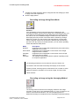
Next you have to log on to your computer. As you can see from the
instructions in the box, pressing the Ctrl, Alt and Delete keys at the
same time will log you on.
After pressing the Ctrl, Alt, and Delete keys, the Login information
dialog box appears.
Typing your password identifies you as a valid user for this computer.
The default user name for the Leica TCS SP2 system is "TCS_User."
A standard password was not set. It is recommended setting up a
separate user ID for each user (system administrator). This will create
individual directories that can be viewed only by the respective user.
Since the LCS software is based on the user administration of Windows
TM
NT , separate files are created for managing user-specific profiles of
the LCS software. For information about setting up users under Windows
TM
NT , please refer to the chapter "Setting Up Users under WinNT" in this
manual.
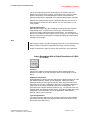
After logging on with your user ID, you may change your password by
pressing the keys Ctrl, Alt, and Delete at the same time.
Then click on Change Password. The Change Password dialog box
displays.
Type your current password in the Old Password field (passwords are
case sensitive, so be sure you use the right case). Then press the Tab
key. Pressing the Tab key moves the cursor to the next field.
Type your new password, then press the Tab key again. Confirm your
new password by re-entering it. This will eliminate any typing errors. This
is especially important since the characters you type appear as asterisks
on the screen.
Note
If you miss-type the confirmation password, you will see a warning
dialog. Try again!
Then click the OK button. Your new password will be in effect the next
time you log on.
Caution
Do not forget your password if you set one! Without the right password
you cannot access your computer anymore.
The Welcome dialog box is now displayed. Take a moment to read the
"Did you know..." tip and then click the Close button to begin using
Windows NT.
Using a Mouse
You need a mouse to work most efficiently in Windows NT. Here are the
mouse actions you need to know:
Point means to move the mouse pointer onto the specified item by
moving the mouse. The tip of the mouse pointer must touch the item.
User Manual Leica LCS english
Art.No.: 15-9330-033 / Vers.: 01082001
Page 7 of 164
Leica Microsystems Heidelberg GmbH
LCS Software Functions
Click on an item means to move the pointer onto the specified item and
press and release the mouse button once. Unless specified otherwise
(i.e. right-click), use the left mouse button. Clicking usually selects an
item.
Double-click on an item means to move the pointer to the specified
item and press and release the left mouse button twice quickly. Doubleclicking usually activates an item.
Drag means to move the mouse pointer onto the item, hold down the
mouse button, and move the mouse while holding down the button.
Unless specified otherwise (i.e. right-drag), use the left mouse button.
The Windows NT Interface
The basic interface of Windows NT is called the "Desktop". It provides a
background for the items it contains.
The initial icons on the desktop allow the user to view and interact with
the system in a logical way.
The Windows NT screen contains many special elements and controls.
Here is a brief summary:
The background on which all the pictures and boxes rest, is the desktop.
The taskbar shows the windows and programs that are open. You can
switch between open windows and programs by clicking the name on the
taskbar.
The Start button opens a menu system from which you can start
programs. Click on the Start button, then click on your selection from
each menu that appears.
Some icons appear on your desktop. You can activate one by double
clicking on it.
We now take a brief tour of the items you see on the screen.
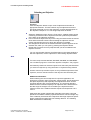
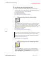
A standard desktop item is the My Computer icon. Double-clicking this
icon opens the My Computer window.
The 'My Computer' window gives you easy access to the major
components like hard and floppy disk drives of your computer system or
workstation. For example, by double-clicking the Hard disk [C:] icon you
can see the contents of your PC's hard drive. This allows the user to view
local resources as objects. The Windows NT Workstation 4 control panel
and print control/support are also accessible from 'My Computer.' If you
installed one of the additional applications such as 'Dial-Up Networking'
at installation time, it will also appear in the 'My Computer' window.
You can use the Control Panel icon in the 'My Computer' window to
view and change any system component. The Control Panel contains
numerous icons that allow you to control your system. The particular
icons that you see on your PC may be slightly different from those
illustrated, due to that fact that you may have different hardware installed,
and may or may not be connected to a network or modem. You may also
have different Windows NT Workstation 4 options installed.
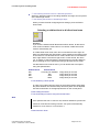
Double-clicking the Network Neighborhood icon displays the Network
Neighborhood dialog box which gives you information about who and
what is connected to your workstation. It provides an easy mechanism for
browsing any network systems and resources that you may be able to
connect to in a way that is independent of the actual type of network
vendor. Traditionally, if a system needed to be simultaneously connected
to different types of network, the way in which each could be connected
and viewed would be vendor-specific. Windows NT Workstation 4 is
capable of displaying a common view of your entire network even though
it may actually comprise resources from Windows NT, Novell NetWare,
Banyan Vines, or others!
The Inbox icon is used if Microsoft Exchange is active on your system.
Windows NT Workstation 4 has built-in electronic mail services based on
User Manual Leica LCS english
Art.No.: 15-9330-033 / Vers.: 01082001
Page 8 of 164
Leica Microsystems Heidelberg GmbH
LCS Software Functions
Microsoft Mail (MS Mail) and Microsoft Exchange. If there is already an
MS Mail post office on the same network that the system is connected to,
the Windows NT Workstation 4 mail client can connect directly to it. The
Inbox lets you access your messages.
The Recycle Bin icon represents the holding place for deleted items. As
long as files are in the Recycle Bin they can easily be recovered if they
have been accidentally deleted. Windows NT Workstation 4 will preserve
files until the system runs out of free disk space. When this happens
Windows NT Workstation 4 will prune the contents of the Recycle Bin on
a first-in first-out basis.
Caution
Files that are overwritten due to an application using a duplicate filename
will not be saved to the Recycle Bin.
Double-clicking the Bin displays its contents. The empty window confirms
that there are no items in the Recycle Bin.
The Start Menu
A single click of the left mouse button on the Start button opens the start
menu and presents the seven major option categories for starting work
on the system.
A single click of the right mouse button opens a small but powerful
control menu containing the options Open, Explore and Find.
Their functionality is described below.
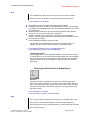
Starting a Program
The Start menu contains the various categories where your applications
and work are stored. You can move further into the various
subcategories by positioning the mouse over the category that you are
interested in to automatically open the next subcategory. You do not
have to click the mouse!
The Programs command displays the Programs menu. This menu lists
all of the applications installed and available to you. Some options are
marked by an arrow. This arrow indicates that a submenu follows. Drag
the mouse cursor over the Accessories command to see its submenu.
The Accessories submenu lists the set of Windows NT built-in programs.
TIP: If you drag an object either from the Desktop or Windows Explorer
and drop it directly onto the Start button, a link to that object will
automatically appear in the Start menu.
There are many ways to start a program. The following method is the
simplest one:
1. Click on the Start button.
2. Click on Programs.
3. Click on the group that contains the program you want to start (for
instance, LCS).
4. Click on the program you want to start (for instance, Leica LCS).
Another way to start a program is to open a document that you created in
that program. The program automatically opens when the document
opens. Double-click on a document file in My Computer or Windows
Explorer to open it. Or click on the Start button and select a recently used
document from the Documents menu.
You can also start a program by double-clicking on its shortcut icon on
the desktop. Shortcut icons are links to other files. When you use a
shortcut, Windows simply follows the link back to the original file.
Whenever you use a document or program frequently, you might
consider creating a shortcut for it on the desktop. To do so, just use the
right mouse button to drag an object out of Windows Explorer or My
User Manual Leica LCS english
Art.No.: 15-9330-033 / Vers.: 01082001
Page 9 of 164
Leica Microsystems Heidelberg GmbH
LCS Software Functions
Computer. After releasing the mouse button, a menu appears. Select the
option Create Shortcut(s) Here. Some programs automatically create a
shortcut during their installation procedure.
Caution
Windows NT Workstation 4 does not actively track a link between an
original and a shortcut. For instance, if you create a shortcut of a
program, and subsequently move (rather than copy) the original to a
different folder, then the shortcut may no longer function.
The Startup folder is special in one respect: any programs located in this
folder will start automatically when Windows NT Workstation 4 is started.
The Documents menu shows the names of the 15 files you created most
recently. You can open any of these files and its related application at the
same time by clicking the file's name in this menu.
Caution
Document files that are opened within an application (typically by
selecting the File/Open command within the application) will not be
displayed here. Only documents opened directly from the Desktop will be
displayed here.
The Settings menu offers three commands for changing your system's
settings. You can directly access the Control Panel and Printing folders.
Also accessible is the Task Properties window.
Being able to access the core system configuration utilities in this way is
particularly useful when an application is already in the foreground and
you want to make a quick change.
The Find command features an easy way to locate all system resources.
Within the Find category you can perform searches for three distinct
types of search as described below:
The Taskbar
The taskbar–positioned at the bottom of the screen–provides a constant
view of which applications are running on the system and an easy way of
switching between them. As you add to the number of concurrently
running applications, the taskbar automatically re-sizes its iconized view
of the applications to ensure that they can always be seen. To switch
from one running program to another, simply click on the second
program as displayed in the taskbar.
The taskbar also provides constant additional information such as the
system time and volume control if a sound card is installed. All of these
functions can be adjusted by the user.
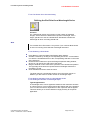
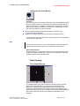
Setting the Time and Date
The current Date, Time and Time Zone information can be set from the
Date/Time icon within the Control Panel. This setting is important since
Windows NT stamps the date and time on all of your files as you create
and modify them. The two options can be selected by clicking on the
appropriate tab.
To change the Date and Time
Click on the appropriate date or use the controls to change the month or
year. The time can also be changed by first selecting the digital display
and then using the up and down arrows.
To change the Time Zone
Select the appropriate Time Zone from the drop down list at the top of the
User Manual Leica LCS english
Art.No.: 15-9330-033 / Vers.: 01082001
Page 10 of 164
Leica Microsystems Heidelberg GmbH
LCS Software Functions
screen. Notice that the option to automatically adjust the clock for
daylight savings time is selected. On some systems you can also drag
the highlighted area on the world map and drop it on the correct location.
Changing the date and time information within Windows NT Workstation
4 will update the battery backup CMOS clock in your system.
Note
Depending on the shell configuration, systems connected to a network
may get a time and date update from a network server every time they
log on. If the server's time is incorrect, your workstation's time will be
wrong, too. Please inform your network administrator.
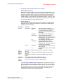
Getting Help
Windows NT includes a powerful help system. In addition to Help menus
in every window, there is a standalone Help feature available from the
Start menu. To access it, click your mouse on the Start button, and click
on Help.
There are three tabs in this box: Contents, Index, and Find. The Contents
tab appears on top. To move to a tab, click on it.
Contents
The Contents tab displays individual Help topics. The topics are
organized into categories and are represented by small book icons.
Double-click on any book to open it. Sub-books and documents appear.
Double-click on sub-books and documents to open them.
Index
The Index tab displays an index of all available topics. Type the word you
want to look up. The Index list scrolls to that part of the alphabetical
listing. When you see the topic on the list that you want to read, doubleclick on it.
Find
Rather than searching for information by category, the Find tab offers a
full text search. Enter the word(s) or phrase to be searched for under
Help in the text entry box. The text entry box is linked to a list of words in
your Help files, and any words or phrases that match will be displayed.
You can specify more than one word by separating words with a space. If
you wish to change a search option, select Options. The first time you
click on this tab, Windows tells you it needs to create a list. Click Next
and then Finish to allow this. The main Find tab appears next. Type the
word(s) you want to find in the top text box. Then click a word in the
middle box to narrow the search. Finally, review the list of help topics at
the bottom, and double-click the one you want to read.
When you're done reading about a document, click Help Topics to return
to the main Help screen, or click Back to return to the previous Help
topic. Click the window's Close button to exit Help.
Shut Down Windows NT
Always use the Shut Down command before you turn off your PC. The
Shut Down option allows the user to close the Windows NT Workstation
operating system and ensure all running processes can halt cleanly and
are given the chance to flush any data out to the disk that may be in
cache memory. Several options are available when shutting the system
down.
User Manual Leica LCS english
Art.No.: 15-9330-033 / Vers.: 01082001
Page 11 of 164
Leica Microsystems Heidelberg GmbH
LCS Software Functions
Caution
Powering down your computer without prior shutting it down may result in
severe data loss.
Setting Up Users Under WinNT
1. Logging on as administrator
Log on as administrator by using the ID "Administrator" and the password
"Admin."
2. Opening the User Manager
Select Start → Programs → Administrative Tools → User Manager.
3. Defining a new user
Enter at least the following information in the opened dialog window:
1. User name
2. Password (must be re-entered in the following line for confirmation
purposes)
Select the following two check boxes:
a.) "User must change password at next logon" (this allows the new user
to define his or her own password at logon)
b.) "Password never expires" (this allows a defined password to be valid
either until it is changed in the User Manager or the user is deleted)
Select the "Profiles" option in the bottom section of the dialog. In the
"Local path" field enter the following path for storing user-specific files:
d:\users\username ("username" is an open parameter which must be
replaced by the currently defined user name).
Note
Factory installed hard disks feature 2 partitions (C:\ and D:\).The user
directory should be set up on partition D:\.
User Manual Leica LCS english
Art.No.: 15-9330-033 / Vers.: 01082001
Page 12 of 164
Leica Microsystems Heidelberg GmbH
LCS Software Functions
The Leica Confocal Software:
Overview
Starting the Software
Requirements for Starting the Software
The LCS software is copy-protected to prevent it from being used on two
computers at the same time. This protection system allows all additional
application packages to be used. The protection system consists of a
dongle that must be inserted into the parallel port of the workstation. The
functionality of the parallel port (e.g., for printing, etc.) is not affected. To
use the software on a second computer, the dongle must be attached to
its parallel port.
Note
If you remove the dongle from the workstation of the confocal system, the
software cannot be started, thereby preventing operation of the confocal
system.
The LCS software can be started in two operating modes: hardware
mode and simulation mode. In hardware mode, all hardware components
are accessed and initialized by the software. For this reason, you should
switch on the hardware first and then wait about 20 seconds before
starting the software.
In simulation mode, the software runs independently of the hardware.
This mode is intended for secondary installations on another computer,
for example for training or offline analysis of existing data.
Starting the Software
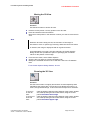
Select Start|Programs|Leica Confocal Software. The initial screen of
the Leica Confocal Software appears. This window allows you to select
from three profiles.
Company
This option starts the Leica Confocal Software using the default factory
settings. This means that the configuration and the position of the
Toolbars is preset. These settings cannot be changed.
Personal
This option lets you use a user-defined configuration profile. The user
name is dependent upon the account used to log on to the operating
system. If the custom profile does not yet exist at the first initialization,
the default factory settings are applied to the personal profile.
Last Exit
This option loads the configuration profile that was last active.
For advanced users:
If you have more than one configuration profile, you can load them at
startup by clicking the button with the three black dots, which is located at
the right lower edge of the profile options. You may also use this option
to reset your custom configuration profile to the standard factory profile.
Clicking the Start button starts the Leica Confocal Software using the
corresponding configuration profile.
Note
After a delay, the software starts automatically and loads the currently
selected configuration profile.
User Manual Leica LCS english
Art.No.: 15-9330-033 / Vers.: 01082001
Page 13 of 164
Leica Microsystems Heidelberg GmbH
LCS Software Functions
The Experiment Software Concept
The Leica Confocal Software allows you to join image data or edited
images into groups. Each group is called an "experiment" and is stored in
a special data format (*.lei). This makes it possible to store both the
original experimental image data and the image viewing data together.
Additional information can be found in the chapter "Organizing Data by
Grouping Experiments"
The Basic Structure of the User Interface
The appearance of the Graphical User Interface–henceforth referred to
as GUI–depends strongly on the configuration profile being used. A
number of elements of the GUI, however, are standard.
The GUI provides the following standard elements:
The menu:
The menu contains the submenus File, View, Macro, Tools, Window and
Help. The submenus contain commands and information for general
display, settings and user customization. They do not provide any of the
functions for directly controlling the scan functions. These functions are
located in the TCS menu (View → Menu → TCS Menu). The menu line
cannot be customized.
The Viewer window (TCS_Viewer):
The Viewer window displays the image data, experimental conditions and
user data. The image window can be configured (see the chapter on
"Modifying the User Interface and Defining User-Specific Settings"). The
image window shows not only the confocal image data records, but also
the experiment data and system settings. You can open a new
experiment image window by selecting File → New.
The TCS menu (TCS_Menu):
The TCS menu contains buttons for the individual device functions. It is
subdivided into individual work steps. The number of work steps
available depends on the installed software. The standard set of work
steps consists of data recording (Acquire), image viewing (View), surface
reconstruction (3 D), measurement functions (Quantify), image
processing and analysis functions (Process), and documentation
functions (Annotate). If the TCS menu is not displayed using the current
configuration profile, you can activate it by selecting View → Menu →
TCS Menu.
The toolbars:
This area allows you to insert and customize individual (function) buttons.
The advantage of the container is that it can be switched on or off with its
entire contents of buttons. To do so, select View → Menu → Container.
The document viewer window (Experiment Overview):
The document viewer window displays the recorded experiments and
their contents in a directory tree. Open this viewer window by selecting
View → Experiment Overview.
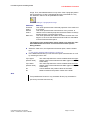
The status bar:
The status bar is found at the bottom edge of the Leica Confocal
Software user interface. It displays:
• the progress while loading image data (progress bar)
• the version number of the software
• the name of the system configuration (system type)
For details about these functions, refer to the chapter on "Software
Reference".
User Manual Leica LCS english
Art.No.: 15-9330-033 / Vers.: 01082001
Page 14 of 164
Leica Microsystems Heidelberg GmbH
LCS Software Functions
Opening Data Records
Readable File Formats
The following file formats can be opened and viewed in the Leica
Confocal Software:
Experiment (*.lei):
The format of this type of file is Leica-specific and binary. This format is
provided for the data of entire experiments.
Tiff files (*.tif):
These are Leica image files in single and multi TIFF format. Both image
files in the previously used TCS formats and external files in RGB TIF
format can be read.
Annotation (*.ano):
The format of this type of file is also Leica-specific and binary. It is used
for saving annotation sheets. The elements on the annotation sheet,
such as images, texts and graphic images, are each available as
individual objects.
When these files are loaded, both the image data and the experiment
settings are loaded.
Automatically Applying the Study Parameters of an Experiment
With the Leica Confocal Software, hardware settings that have been
saved for previous experiments or single images can be applied to new
experiments. This allows you to carry out different experiments using
constant settings. To carry over settings from a previous experiment,
open the viewer window for the data record that contains the settings you
want to apply. There, click the "Apply" button, which, in the factory default
configuration profile, is located in the toolbar.
Note
If you do not find the "Apply" button in one of the open windows, you can
load it into any of the windows by selecting Tools → Customize. In the
dialog window that appears, select the "Commands" tab under the File
category. With the left mouse button, click the "Apply" button and drag it
while holding the mouse button pressed to the desired window. Release
the left mouse button to insert the button at the current location.
Saving Images
As described above under "Readable File Formats", individual images
and experiments can be saved using the same data formats.
Select File → Save to save your images and experiments. The first time
an experiment is saved, the "Save as" dialog opens automatically,
allowing you to specify a file name. In addition to defining a suitable file
name, you can also select a file format here. Experiments can only be
saved in the Leica-specific *.lei format. When you are saving
experiments, you may be able to save existing individual images in *.tif or
*.raw format.
Note
If you are saving an experiment or image that has already been saved
before, the old data will be overwritten.If you do not want to do this,
select File → Save as to save the new or changed data to a new file with
a new name.
User Manual Leica LCS english
Art.No.: 15-9330-033 / Vers.: 01082001
Page 15 of 164
Leica Microsystems Heidelberg GmbH
LCS Software Functions
Data Organization by Grouping Experiments
The concept of the Leica Confocal Software allows you to group
individual images, image series and the results of edited images into
single groups, or experiments. The Experiment Overview window
provides a general overview of the open experiment. To open the
Experiment Overview window, select View → Experiment Overview.
Create a new experiment by selecting File → New or File → New
(Template). Files that were previously saved are handled as separate
experiments when opened.
Compiling Experiments
Note
After you have defined a new experiment by selecting File → New or
File → New (Template), you can start filling it with data.
Images that have been recorded in continuous scan mode are
overwritten automatically when the next scan is started. If you want to
keep a single recording as a permanent part of an experiment, you
should use the single scan function.
An experiment contains data acquired with the "single scan" or "series
scan" function. If you carry out image processing functions on a data
record, you can save the results as additional components of the
experiment. To do this, double-click the desired image or series in the
experiment overview window. Carry out the desired image processing
functions (such as maximum projection or topological image or others).
Mark the region within the viewer window that you want to keep as part of
the experiment. Click the right mouse button (to open the context menu)
and select Send to → Experiment. The Selection (raw) option stores a
copy of the raw data of the selected object as a new, separate
component of the experiment. The Selection (snapshot) option stores
an RGB image (no 3D data, just a pure snapshot) of the selected object
as a new, separate component of the experiment.
Menu Functions
The following TCS SP2 functions can be carried out from the menu bar:
File Menu
New:
This option opens a new experiment in a new window. The display
properties of the new window are determined by the active defaults (see
the chapter on "Default Settings and Templates").
New (Template):
This option opens a new experiment in a new window. The way in which
the viewer window is displayed can be selected from a set of templates.
Open:
This option opens a previously saved experiment or a single data block
(image data or annotation). The display properties of the new window are
determined by the active defaults (see the chapter on "Default Settings
and Templates").
Open (Template):
This option opens a previously saved experiment, a single data block or
annotation files. The way in which the viewer window is displayed can be
selected from a set of templates.
Close:
User Manual Leica LCS english
Art.No.: 15-9330-033 / Vers.: 01082001
Page 16 of 164
Leica Microsystems Heidelberg GmbH
LCS Software Functions
This option closes the current experiment. It does not save the
experiment automatically before closing it.
Note
You are not asked whether you want to save the experiment before it is
closed.
Close all:
This option closes all open experiments. It does not save the experiment
automatically before closing it.
Note
You are not asked whether you want to save the experiment before it is
closed.
Save:
Saves the current experiment.
Recent files:
Opens one of the recently opened files.
Print:
Opens a dialog for printing the content of the currently active window.
Exit:
Terminates the program.
The View Menu
Menus:
Use this option to switch TCS menu and the toolbar on and off.
Status bar:
This option switches the display of the status bar on and off at the bottom
edge of the user interface of the LCS software.
Experiment Overview:
This option opens a window displaying the individual experiments and
their components (data records, graphs, etc.) in the form of a tree.
Double-click an experiment component within the Experiment Overview
window to bring the corresponding viewer window to the foreground.
Viewer Options:
Use this item to configure various options for displaying data records in
the viewer window, such as the display angle and calculation methods for
displaying image data, etc.
The Macro Menu
Macros:
Depending on the software installed, either use this option to edit macros
directly or just list and run them.
Note
You can edit and modify macros only if the complete, integrated VBA
development environment (IDE) is installed.
Record a New Macro:
This starts the automatic macro recorder. For more information, refer to
the documentation provided with the optional macro development
environment.
Pause Recording:
This pauses the macro recorder.
Stop Recording:
This stops the macro recorder.
Visual Basic Editor (optional):
This option launches the software for developing macros and programs
User Manual Leica LCS english
Art.No.: 15-9330-033 / Vers.: 01082001
Page 17 of 164
Leica Microsystems Heidelberg GmbH
LCS Software Functions
based on Visual Basic for Applications (VBA). Here you can edit and
modify macros and even develop entire programs.
The Tools Menu
Legend Info:
This option opens the dialog window for entering user-specific data. This
data (e.g., name of institute, name of specimen, etc.) is saved with each
data record and can be displayed next to the acquired images in the
legend.
Objective:
This option opens the dialog window for defining applied objectives. The
objectives you use can be made known to the software by copying them
using "drag and drop" from the list provided in this dialog window.
Note
It is important to apply the correct data for the objectives, as some of the
calculated sizes (such as the scan field dimensions) depend on them.
Microscope:
Use this option to select the Leica microscope you are using. This setting
influences the way in which the microscope is controlled (for example,
the motorized objective nosepiece).
Settings:
Use this option to select the hardware settings that you want to be
applied when opening a previously saved data record.
License:
This option allows you to install subsequently purchased licenses. A
subsequent license usually is installed if a software package offered as
an option is purchased.
The Window Menu
New Window:
This option opens a new viewer window within the same experiment. For
example, you can use this function to view the same data record using
different views (such as topographical and overlay views).
The Help Menu
Contents:
Opens the table of contents of the online help.
Search:
Starts the search function for the online help.
Index:
Opens the index of the online help.
User Manual Leica LCS english
Art.No.: 15-9330-033 / Vers.: 01082001
Page 18 of 164
Leica Microsystems Heidelberg GmbH
LCS Software Functions
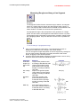
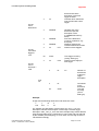
Keyboard Shortcuts
Special key combinations have been defined to speed up access to
frequently used software functions.
Keyboard
Shortcuts
F1
ALT + F8
ALT + F11
(optional)
CTRL + L
CTRL + J
CTRL + N
CTRL + O
CTRL + P
CTRL + S
Function
Opens the online help.
Opens the Macros dialog window for running, editing and
deleting macros.
Starts the VBA development environment (optional).
Opens the Legend Info dialog window for entering userspecific settings that can be applied when documenting,
saving and viewing the documentation of image recordings.
Opens the Objective dialog window for defining and selecting
applied microscope objective lenses.
Opens a new experiment.
Starts the Open dialog window for opening an existing file.
Opens the Printer Selection dialog window.
Saves the active experiment.
LCS Software Functions
Introduction to the Leica Confocal Software Help
Three different help levels are available for the Leica TCS SP2:
Quick Help
When you let the mouse pointer hover over a Leica Confocal Software
button, a brief explanation of the function of this button is displayed. This
so-called Help Banner automatically disappears when the mouse pointer
is moved.
Context-sensitive Help
If you want to use the context-sensitive help function, click on the Help
button:
The entire user interface is then frozen and a question mark appears
beside the mouse pointer. Then, instead of triggering the button function,
clicking a button opens an explanation of the button's function. If the Help
button is not present on the user interface:
K
K
K
Select the Customize option from the Tools menu. Here you will find all
buttons arranged by categories.
The Help button can be found in the File category.
Click on it using the left mouse button and drag it to the desired window.
Contents of the Online Help
Select the Contents option from the Help menu to view the online help
table of contents, which allows you to select any function in order to view
information on it.
User Manual Leica LCS english
Art.No.: 15-9330-033 / Vers.: 01082001
Page 19 of 164
Leica Microsystems Heidelberg GmbH
LCS Software Functions
Keyword Search (Index)
Select the Index option from the Help menu to view an index of key
words. Select a key word. View the corresponding content pages by
double-clicking the key word or selecting it and then clicking the Display
button.
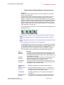
Full-text Boolean Search
Select the Search option from the Help menu to launch the full-text
search engine. Enter your search word in the input field. Click the triangle
to the right of the input field to view the available logical operators. Select
the desired operator. Enter the second search word you would like to
associate with the first search word behind the operator:
Examples
Pinhole AND
Sections
Pinhole OR
Sections
Pinhole
NEAR
Sections
Pinhole NOT
Sections
Result
This phrase finds help topics containing both the word
"pinhole" and the word "sections".
This phrase finds help topics containing either the word
"pinhole" or the word "sections" or both.
This phrase finds help topics containing the word "pinhole" and
the word "sections" if they are located within a specific search
radius. This method also looks for words that are similar in
spelling to the words specified in the phrase.
This phrase finds help topics containing the word "pinhole" and
not containing the word "sections".
Favorites
If you select Favorites in the dialog window of the online help tab, you
can include the current help topic in a list, making them easily available
for future use.
Opening the Context-Sensitive Help
Function
Click Help to open the context-sensitive online help function, which
provides you with short explanations for the various buttons and
functions of the Leica Confocal Software.
K
K
K
K
Click the Help button.
A question mark appears next to the mouse pointer. This temporarily
disables the functions of all buttons.
Use the mouse pointer to click the button that you want an explanation of.
Online help opens directly to the description for the corresponding button.
Online help also provides you with an index of key words and a search
function so that you can search for specific topics and buttons.
Furthermore, you can print the individual descriptions.
You can also open the online help by selecting Contents, Search or
Index option under the Help menu.
User Manual Leica LCS english
Art.No.: 15-9330-033 / Vers.: 01082001
Page 20 of 164
Leica Microsystems Heidelberg GmbH
LCS Software Functions
Documentation Conventions
Button
The buttons provided on the user interface of the Leica Confocal
Software. Buttons are marked with icons and/or have an (often
abbreviated) English label. They either trigger actions directly or open
dialog windows.
Menu
The menus are divided into the categories of File, View, Macro, Tools,
Window and Help and are displayed in the menu bar located at the upper
edge of the user interface.
Option
Options refer to the selectable items that are hierarchically listed below
the menus. Options either trigger actions directly or open dialog windows.
Dialog Window
Both buttons and options open dialog windows. Dialog windows are used
to set various parameters and select functions.
Register
Registers are found in dialog windows. Registers thematically combine
the parameters and functions that can be configured in dialog windows.
Some registers are divided into fields.
Viewer window
The Leica Confocal Software contains two types of viewer window. The
Viewer window is called up by pressing the New button and displays the
recorded images. The Experiment Overview viewer window displays the
recorded images in a directory tree. This viewer window is called up from
the View menu and appears as a separate window at the left side of the
user interface.
Legend
The Leica Confocal Software provides two legends, which display the
parameters and settings of an image recording. The Experiment legend
can be placed at the right edge of the Viewer window. The Hardware
legend is called up from the View menu and appears as a separate
window at the left side of the user interface.
Context Menu
Context menus appear when you click the right mouse button while
holding the mouse pointer over certain areas of the user interface.
Context menus contain various, context-sensitive commands.
see ...
This symbol is a reference to another topic in the online help.
User Manual Leica LCS english
Art.No.: 15-9330-033 / Vers.: 01082001
Page 21 of 164
Leica Microsystems Heidelberg GmbH
LCS Software Functions
Data Recording
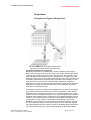
Setting the Beam Path
Function
Open the Beam Path Setting dialog window using the Beam button, and
set up the beam path and the detectors with the corresponding color
look-up tables used to record the image.
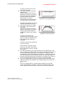
Selecting the excitation wavelength
Above the spectrum in the dialog window you will find boxes to set the
excitation wavelength using an AOTF:
K
K
K
K
Click the check box next to the laser name to activate the laser.
Set the output for the laser line by moving the slide on the corresponding
scale to the desired value, or
Double click the percentage value for the laser output. This opens a
second dialog window where you can enter an exact value.
The active laser line is shown as a line in the spectrum.
Loading and Saving Parameter Settings
Also above the spectrum is a list box for loading and saving parameter
settings. The manufacturer has predefined parameter settings for the
most important fluorescent dyes. They are labeled with the letter L (for
Leica) and can be loaded only, not modified.
You can also save the settings made for a specific image recording as
user-defined parameter configuration so that you can load them any time
with a single click:
K
K
K
Click the Save button.
This opens a dialog window for entering a name for the parameter
configuration.
The parameter configuration is stored in the list box under User and is
labeled with the letter U (for User).
Furthermore, you can individually select the parameters that you want
saved when using the Save command:
K
K
K
Select the Settings option from the Tools menu.
In the Settings dialog window, click the Instrument Parameters tab.
Select individual parameters by clicking the corresponding checkboxes.
The Select all and Deselect all buttons allow you to select all or no
parameters quickly.
Click one of the user-defined or preset parameter configurations and then
press the right mouse button to open a context menu, which contains the
following commands:
User Manual Leica LCS english
Art.No.: 15-9330-033 / Vers.: 01082001
Page 22 of 164
Leica Microsystems Heidelberg GmbH
LCS Software Functions
Command
Set as default
setting
Remove default
setting
Load
Rename (only for
U)
Delete (only for U)
Function
The standard setting for the parameters is loaded when
you start the software.
This removes the default setting property from the
selected configuration.
Loads the parameter configuration.
Use this to change the name of the parameter
configuration.
Deletes the parameter configuration.
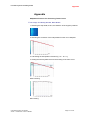
Selecting the excitation beam splitter
The symbol (green, tilted line) for the excitation beam splitter is located to
the left of the spectrum. Click on the symbol and select the desired beam
splitter:
K
K
K
K
Neutral filters, such as the RT 30/70 filter, are used in reflection
applications to lead the excitation light to the sample and the reflected light
to the detection pinhole.
Dichroic filters, such as the reflection short pass filter RSP 510, are used in
fluorescence applications to split and detect fluorescent light of a particular
wavelength range from the excitation light.
Double dichroic filters are used for image recording, where the preparation
is marked with two fluorescent dyes and two excitation wavelengths. The
DD 488/568 double dichroic, for instance, is used to split excitation light
with a 488 nm and 568 nm wavelength from the detection light. Depending
on the system configuration, you can also select DD 488/ 543 and DD 458/
514 type double dichroites.
Triple dichroic filters are used for image recording, if the preparation is
marked with three fluorescent dyes and three excitation wavelengths. The
TD 488/568/633 triple dichroic, for instance, is used to split excitation light
with a 488nm, 568nm, and 633nm wavelength from the detection light.
Depending on the system configuration, you can also select TD 488/ 568/
647 and TD 488/ 543/ 633 type triple dichroites.
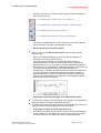
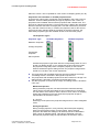
Setting detectors and color look-up tables (LUT)
Below the spectrum in the dialog window the boxes for the four detectors,
PMT 1 to 4, as well as for the PMT Trans transmitted light detector are
shown. Adjust the settings as follows:
K
K
K
K
K
Activate each of the desired detectors by clicking on its corresponding
Active check box below the color look-up table icon. A cast shadow now
links the activated detector to the corresponding slide bar on the scale of
the spectrum.
Specify the wavelength range for the detection by dragging the two ends of
the slider to the desired positions on the scale, or
Double-click the slide bar to open an additional dialog window in which you
can enter a precise value for the start point and the end point of the
wavelength range.
For fluorescence applications, list fields with common fluorescence dyes
have been set up for each detector. Select the desired fluorescence dye to
display its emission curve in the spectrum.
Select a color look-up table by clicking on the corresponding icon.
see Selecting Color Look-Up Tables
User Manual Leica LCS english
Art.No.: 15-9330-033 / Vers.: 01082001
Page 23 of 164
Leica Microsystems Heidelberg GmbH
LCS Software Functions
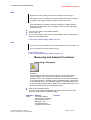
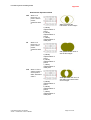
Selecting an Objective
Function
Click the Objective button to open a list of objectives and make an
appropriate selection. This list contains only the objectives that were
previously assigned to one of the maximum of seven threaded ports on
the objective nosepiece. You can assign objectives as follows:
K
K
K
K
Select the Objectives option from the Tools menu. A dialog window opens
containing an extensive list of objectives and the symbolic representation
of the slots on the objective nosepiece.
Find in the list the objective that you are using and select it with the mouse.
Click and hold the left mouse button and drag the objective onto the
symbol representing the slot in which the objective is installed.
The assignment is saved in the software and the objective appears in the
selection list, which you can open by pressing the Objective button.
Repeat this procedure for every objective that you have installed in the
objective revolver.
You can use the Add, Remove and Edit buttons in this dialog window to
add new objectives, remove objectives or edit existing objective labels.
Note
The microscope models DM RXA, DM RXE, DM IRBE, and DM IRBE2
use a software program to control the objective nosepiece. The program
automatically rotates the selected objective into the beam path whenever
you select an objective by using the button or Objective dialog window.
All other microscope models require not only software adjustment of the
objective, but also manual rotation of the objective into the beam path.
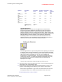
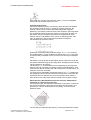
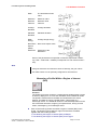
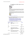
Additional information
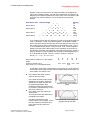
When selecting the correct objective for a specific application, the
objective's correction class (achromatic, apochromatic, fluorite objectives
and plane objectives) and especially the magnification factor and the
numerical aperture are of great significance. The numerical aperture
determines the resolution capacity of an objective and is deduced from
the flare angle of the light cone recorded by the objective and the
refraction index of the medium between objective and specimen: NA =
n*sin a
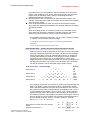
Objectives with greater magnification generally have larger numerical
apertures but smaller entrance pupils and therefore can record light only
from a relatively small scan field. Objectives with larger apertures permit
higher resolutions but allow less free working distance. The following
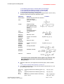
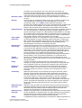
table illustrates this relationship:
User Manual Leica LCS english
Art.No.: 15-9330-033 / Vers.: 01082001
Page 24 of 164
Leica Microsystems Heidelberg GmbH
LCS Software Functions
Objective
Resolution
(xy)
Resolution
Air (z)
Resolution
Water (z)
Resolution
Oil (z)
HC PL
FLUOTAR 5x
0.15
HC PL
FLUOTAR 10x
0.30
N PLAN 20x
0.40
N PLAN 50x
0.75
PL APO 100x
1.40
1301
19410
25879
29559
Scan
Field Size
(xy)
3000
651
4768
6407
7335
1500
488
2630
3566
4093
750
260
649
948
1108
300
139
319
209
236
150
Values in nm at
wavelength λ=488
nm
Values in
mm
Typical Applications
Material scientists commonly use dry objectives to study surface
structures. Immersion Objectives are the best choice for producing
images of layered structures in which material layers with varying
refraction indexes come into contact with each other. When working with
biological specimens, the choice between an oil immersion objective and
water immersion objective depends on the specimen itself and its
embedding medium. You will achieve the best resolution when the
refraction indexes of the embedding medium and/or the specimen are
matched to the refraction index of the objective medium.
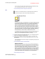
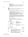
Setting the Detectors
Function
Use the Signal button to open a dialog window for adjusting the detectors
so that the entire range of intensities of a color look-up table is assigned
and displayed in the image. For this purpose, a Gain value and an Offset
value can be set for each detector. The gain value modifies the
amplification of the detected signal, thus changing the brightness and
contrast of the image. The offset value defines a threshold value. Only
those signals that lie above the threshold value are detected and
displayed in the image.
There are two methods for setting the gain and offset values:
K
K
Use the mouse to move the slide on the scale. The corresponding value is
shown below the corresponding scale.
Double-click the numerical value that is displayed below the scale. This
opens a second dialog window where you can enter an exact value.
Best suited to optimization of gain value and offset values are the color
look-up tables Glow Over, Glow Under and Glow Over and Under.
see Selecting Color Look-Up Tables
User Manual Leica LCS english
Art.No.: 15-9330-033 / Vers.: 01082001
Page 25 of 164
Leica Microsystems Heidelberg GmbH
LCS Software Functions
You can also set the gain value and offset value of the detectors using
the corresponding radio buttons of the control panel.
see Controlling Functions Using the Control Panel
Note
A detector is not enabled unless its corresponding Active checkbox is
checked in the Signal or Beam Path Setting dialog windows.
The Electronic Zoom
Function
In confocal microscopy, the magnification of an image is determined both
by the objective and the electronic zoom. The objective generates a first
image whose magnification is based on the objective's magnification
factor. The electronic zoom provides additional magnification. A zoom
factor of 1 scans the maximum scan field size with a specific number of
dots. If the zoom factor is set to 2, the same number of dots is used to
scan a scan field with half the page length of the maximum scan field (1/4
the original scan field). This achieves stronger magnification and thus
better image resolution too, because a smaller scan field is scanned with
the same frequency, which results in a higher density of data.
In the dialog window that was opened by pressing the Zoom button, you
can select one of the preset zoom factors. If you click on the Others
button, you can set a different zoom factor in two ways:
K
K
Use the mouse to move the slide of the scale. The corresponding value is
shown in the middle of the dialog window.
Double-click the boldface numerical value located in the middle of the
dialog window. This opens a second dialog window where you can enter
an exact value.
You can also set the zoom factor using the corresponding rotary knob on
the control panel.
see Controlling Functions via Control Panel
Additional information
While zoom factors from 1 to 32 can be set, the useful magnification of
the electronic zoom cannot be increased infinitely. The limit is achieved
using the smallest optically resolvable distance, which is determined by
the resolution capacity of the objective. According to the Nyquist
theorem, this smallest optically resolvable distance can only be mapped
without information loss if it is scanned with about 2 to 3 raster points. If
the scan frequency is exceeded at a relatively high zoom factor and the
specified scan format, further magnification is no longer useful because
no more optical details can be resolved (zero-order magnification).
see Selecting a Scan Format
User Manual Leica LCS english
Art.No.: 15-9330-033 / Vers.: 01082001
Page 26 of 164
Leica Microsystems Heidelberg GmbH
LCS Software Functions
see Selecting an Objective
Note
With bleach-sensitive specimens it is advisable to restrict the use of the
electronic zoom to short time intervals. Since you are recording a
segment of the specimen with a relatively higher scan frequency in the
case of high zoom factors, the specimen is exposed to a stronger impact
of light. This can lead to photomechanical destruction of the specimen
(optical bleaching).
Optimal Zoom Factors
The following table shows which zoom factors (marked red) - depending
on the scan field size and scan format specified by the objective that can
be used to scan the specimen without loss of data:
Objective
Magnificatio
n
Numerical
Aperture
20
0,6
Resolution
at λ=488
nm
325
Scan
Format
Zoom
Factor
s
Scan
Field
Size
(mm)
Scan
Frequency
(nm)
Resolution/
Scan
Frequency
1024 x
1024
1
2
4
6
1
2
4
8
10
1
2
4
8
16
32
1
2
4
6
1
2
4
8
10
1
2
4
8
16
32
1
2
3
1
2
4
6
1
2
4
8
12
750
375
187
125
750
375
187
94
75
750
375
187
94
47
23
375
187
94
62
375
187
94
47
37
375
187
94
47
23
12
150
75
50
150
75
37
25
150
75
37
18
12
732
366
183
122
1465
732
365
183
146
3750
1875
935
470
235
115
366
183
92
60
732
365
183
92
72
1875
935
470
235
115
60
146
73
49
293
146
72
49
750
375
185
90
60
0,4
0,8
1,8
2,7
0,2
0,4
0,9
1,8
2,2
0,1
0,2
0,3
0,7
1,4
2,8
0,4
0,8
1,7
2,6
0,2
0,4
0,8
1,7
2,2
0,1
0,2
0,3
0,7
1,3
2,6
0,9
1,9
2,8
0,5
0,9
1,9
2,8
0,2
0,4
0,7
1,5
2,3
512 x 512
200 x 200
40
1,25
156
1024 x
1024
512 x 512
200 x 200
100
1,4
139
1024 x
1024
512 x 512
200 x 200
User Manual Leica LCS english
Art.No.: 15-9330-033 / Vers.: 01082001
Page 27 of 164
Leica Microsystems Heidelberg GmbH
LCS Software Functions
Note
The Leica Confocal Software provides three different zoom functions: the
electronic zoom, the 3D zoom and the graphic zoom.
see Zooming the 3D View
see Viewer Options Dialog Window, Display Icon
Enlarged Recording of a Frame
Function
The Zoom In function enables an enlarged recording of a freely
selectable square frame of a specimen.
K
K
K
K
Click the Zoom In button. At the same time, the Rectangle button is
automatically activated.
see Defining the Region of Interest (ROI) as a Rectangle
Specify the frame to be enlarged by drawing a rectangular evaluation area
(region of interest or ROI) into the image using the Rectangle button.
see Selecting and Moving the Region of Interest (ROI)
Use the Select button to move the frame on the image.
To start the image recording, press the Continuous Scan, Series Scan or
Single Scan button.
Note
The software automatically adapts the freely selected rectangular frame
to the actual square form that can be implemented by the scanner. The
dashed line shows the actual frame.
Additional information
The enlarging recording of a frame will only provide additional detailed
information as long as the distance of the grid points remains larger than
half the optical resolution. On the other hand, the resolution depends on
the objective used, the adjusted scanning format, and the light
wavelength used (Empty magnification).
Typical Applications
All applications that deal with the optical resolution of very small
structures and that can do without an overview image. While recording
such specimens, care should be taken that an objective with a
corresponding high optical resolution is used for image recording.
User Manual Leica LCS english
Art.No.: 15-9330-033 / Vers.: 01082001
Page 28 of 164
Leica Microsystems Heidelberg GmbH
LCS Software Functions
Setting the Detection Pinhole
Function
Clicking the Pinhole button opens a dialog window that you can use to
set the diameter of the detection pinhole. In the upper right list field in the
dialog window, select the units for displaying the diameter. You can
select from mm, Airy units and digital values. There are two ways of
specifying a value for the diameter:
K
K
Use the mouse to move the slide on the scale that is displayed on the left
in the dialog window. The corresponding value is shown in the middle of
the dialog window.
Double-click the boldface numerical value located in the middle of the
dialog window. This opens a second dialog window where you can enter
an exact value.
The diameter of the detection pinhole must be set to the currently used
objective at all times. If you click the Airy 1 button, the detection pinhole
is set automatically to the optimum value of 1 Airy unit depending on the
objective in use.
In addition to the numerical aperture of the objective and the wavelength
of the light, the detection pinhole also determines the thickness of the
optical sections.
Additional information
The diameter of the pinhole has the optimum if it matches the diameter of
the Airy disc. The Airy disc refers to the inner, light circle of the diffraction
pattern of a point light source. The diameter of the Airy disc, in turn, is
also dependent on several optical parameters and can be described for
the Leica Confocal System as follows:
To calculate the diameter of the Airy disc, you need the excitation
wavelength l (in the case of several wavelengths, a mean value should
be used); the numerical aperture NA and the magnifying factor M of the
objective. The factor of 3.6 refers to the magnification of other optical
components belonging to the Leica Confocal microscope.
If the pinhole is set to the Airy disc, light from outside the focal plane is
suppressed and the signal-to-noise ratio is high. These conditions allow
the recording of optical sections of minimum thickness. The wider the
diameter of the pinhole, the more light reaches the detector. The image
becomes brighter but blurring from structures outside the focal plane will
also appear in the image, making it increasingly unfocused.
Increasing the diameter of the pinhole above 1 Airy unit is recommended
only for detecting very weak signals.
Generally when recording material scientific specimens, enough light is
reflected into the detectors so that the detection pinhole can be closed
completely (i.e. set to the minimum diameter).
User Manual Leica LCS english
Art.No.: 15-9330-033 / Vers.: 01082001
Page 29 of 164
Leica Microsystems Heidelberg GmbH
LCS Software Functions
Selecting a Scan Format
Function
Clicking the Format button opens a dialog window containing a selection
list of scan formats. Selecting the scan format selects the image raster
that will be used for recording the images. An image raster is the amount
of points scanning the specimen in the three directions in space. Besides
the numerical aperture of the objective and the excitation wavelength, the
scan format, together with the electronic zoom, determines in large part
the spatial resolution of the recorded data.
Additional information
When selecting the scan format, observe the influences between the
image raster and the resolution of the generated image. According to the
Nyquist theorem (or sampling theorem), a structure can only be scanned
without information loss if the smallest optically resolvable distance is
scanned with about 2 to 3 raster points. This optically resolvable
distance, called lateral resolution, depends on the numerical aperture of
the objective and the wavelength of the applied excitation light:
The following example should illustrate this relationship: You have
selected, for example, the PL APO 100x objective unit with a numerical
aperture of NA = 1.4 and a wavelength of l = 488 nm. Based on these
factors, the smallest optically resolvable distance is determined as
follows:
Based on this rough formula, the distance of the raster points required
avoiding information loss while recording is:
If however you select a scan format of 1024x1024, a PL APO 100x
objective, which has a maximum
Scan field size of 150 mm, would result in the following raster point
distance:
To achieve the required 47 nm raster distance, you can either raise the
scan format (to 2048x2048 for instance) or you can decrease the scan
field size using the Electronic Zoom (Zoom=2).
The current raster distance is displayed in the Hardware legend. This
value is referred to as Voxel Size and recalculated as soon change the
scan format, the Electronic Zoom or the objective.
see The Electronic Zoom
see Selecting an Objective
User Manual Leica LCS english
Art.No.: 15-9330-033 / Vers.: 01082001
Page 30 of 164
Leica Microsystems Heidelberg GmbH
LCS Software Functions
Note
When the sampling rate of 2 to 3 points is exceeded, it is referred to as
oversampling. In the case of oversampling, the structure is fully mapped
but no additional information is gained. The disadvantage of
oversampling is the long scanning time and the danger of destroying
bleach-sensitive specimens. When the sampling rate is less than 2 to 3
points, it is referred to as undersampling. In this case, there is the danger
that not all necessary information is sampled. The image might illustrate
structures that are not actually present in the specimen. This effect is
called aliasing.
Selecting a Scan Mode
Function
Clicking the Mode button opens a dialog window containing a list of
available scan modes. The scan mode determines which optical levels of
the specimen are to be scanned. Fundamentally, horizontal xy-sections
or vertical xz-sections can be recorded. To generate a three-dimensional
image of the specimen, the optical sections are continued in the
corresponding third direction in space, thus recording a stack of
individual images. In addition to this, it is possible to add the factor of
time or wavelength while recording the images:
Mode
xyz
xzy
xt
xyt
xzt
xyzt
xyλ
xzλ
Function
An image stack is recorded from the xy-sections in the z direction.
An image stack is recorded from the xz-sections in the y direction.
A line is recorded several times in succession.
A xy-section is recorded several times in succession.
An xz-section is recorded several times in succession.
An image stack is recorded several times in succession from xysections in z-direction.
An xy section is recorded at different wavelengths.
An xz section is recorded at different wavelengths.
All scan modes (with the exception of xt) are composed of at least three
dimensions. The device will ignore the third as well as other dimensions if
you record images only from one optical plane (xy or xz) using the
Continuous Scan function of the Single Scan function.
User Manual Leica LCS english
Art.No.: 15-9330-033 / Vers.: 01082001
Page 31 of 164
Leica Microsystems Heidelberg GmbH
LCS Software Functions
Note
The xzy and xzt scan modes are only displayed in the list if you
previously selected the selection point Galvo using the Z-Scan button.
Likewise, the scan modes for a xyλ and xzλ wavelength will only be
displayed if only one detector is activated in the Beam Path Setting
dialog window.
see Setting the Beam Path
Selecting a Scan Speed
Function
Clicking the Speed button opens a dialog window that you can use to
select from four scan speeds.
Speed
200
400
800
1000
Image lines per second
Image lines per second
Image lines per second
Image lines per second
The data recording speed is further increased in combination with the bidirectional scan.
see Unidirectional or Bi-directional Scan
Additional information
The higher the set scan speed, the shorter the dwell time of the laser
point. Furthermore, the scan format, i.e. the number of sampling points in
a row, needs to be taken into account. The higher the scan format at a
constant speed is, the shorter the dwell time of the laser point over a
sampling point.
The longer the light point of the laser beam dwells over the individual
sampling points of the specimen, the more light is detected by the
detector. So using a lower scan speed results in a better signal-to-noise
ratio. The disadvantage of a lower scan speed is that the relatively long
impact of the light on the specimen can bleach the specimen
photochemically, making it unusable. This is especially important with
fluorescence applications
Note
If the speed levels 800 or 1000 are set, technical limitations prevent the
maximum scan field from being scanned. The system automatically
switches to zoom factor 2 or zoom factor 4.
User Manual Leica LCS english
Art.No.: 15-9330-033 / Vers.: 01082001
Page 32 of 164
Leica Microsystems Heidelberg GmbH
LCS Software Functions
Setting the Z/Y-Position
Function
Use the z/y-Position button to define the horizontal level (z position) or
vertical level (y position) of the specimen in which the images are to be
recorded. To record an image series using the Series Scan function,
define the start and end points of the image series using the z/y-position
button and the Begin and End buttons.
see the Series Scan Overview Dialog
Clicking the z/y-Position button opens a dialog window that provides you
with two ways of specifying a position value:
K
K
Use the mouse to move the slide on the scale that is displayed on the left
in the dialog window. The corresponding position value is shown in the
middle of the dialog window.
Double-click the boldface position value located in the middle of the dialog
window. This opens a second dialog window where you can enter an exact
value.
The z/y-position can also be set using the corresponding knob on the
console.
see Controlling Functions via Control Console
Configuring a Time Series
Function
Click the Time button to open the Time Configuration dialog window for
setting up a time series recording. The settings that can be changed in
this dialog window depend on the selected scan mode. You can record a
line (xt), a horizontal section (xyt), a vertical section (xzt), or a stack of
horizontal sections (xyzt), interrupted by a particular time interval, many
times in a row.
Note
The Time button is not enabled unless you have selected a scan mode
with time dimension using the Mode button.
see Selecting a Scan Mode
User Manual Leica LCS english
Art.No.: 15-9330-033 / Vers.: 01082001
Page 33 of 164
Leica Microsystems Heidelberg GmbH
LCS Software Functions
Use the following parameters in the dialog window to configure a time
series using the xt scan mode.
∆T
Lines
Lines per
page
Pages
Complete
Time
The recording time for a line (cannot be modified by the user)
Number of line recordings
Number of lines per stored page
Number of stored pages (calculated automatically)
Total recording time, i.e. the product of ∆T and number of
recordings
Using the Calculate button, you can calculate how many stored pages
are needed for a particular number of lines per page.
Use the following parameters in the dialog window to configure a time
series using the xyt or xzt scan mode.
∆T
Frames
Complete
Time
Recording time for a xy-section or xz-section plus pause
interval
Number of recordings of the xy-section or xz-section
Total recording time, i.e. the product of ∆T and number of
recordings
Use the following parameters in the dialog window to configure a time
series using the xyzt scan mode:
∆T
Stacks
Complete
Time
Recording time for a stack of xy-sections plus pause interval
Number of recordings of the image stack
Total recording time, i.e. the product of ∆T and number of
recordings
Each parameter can be calculated in relation to the other parameters.
When entering the values, note how the dialog window operates. The
entry field you click on will be activated:
K
K
K
Click on the parameter to be calculated. The corresponding entry field is
grayed out.
Now enter the values for the other parameter.
Click on Apply to calculate the parameter. By clicking on Reset, the last
saved values are displayed.
When you have finished configuring these settings, press the Series
Scan button.
Starting a Single Scan
Function
Use the Single Scan button to record a single image from a single optical
level in the specimen.
Before recording an image using the single scan function, configure all
User Manual Leica LCS english
Art.No.: 15-9330-033 / Vers.: 01082001
Page 34 of 164
Leica Microsystems Heidelberg GmbH
LCS Software Functions
required scan parameters using the Continuous Scan function to ensure
optimal image quality.
see Starting a Continuous Scan
Typical Applications
The single scan function is designed for recording bleach-sensitive
specimens. Use this function in the case of bleach-sensitive specimens
not only for image recording, but also as an alternative to the continuous
scan function for setting the scan parameters. The single scan function
can also be used to check the image section by zooming in on the scan
field.
Starting a Continuous Scan
Function
Use the Continuous Scan button to permanently record images from a
single optical level in the specimen. This does not generate image series,
since the image being generated always replaces the previously
generated image.
Press the button a second time to stop the continuous scan.
Additional information
The unit applies the last used scan parameters automatically. You can
modify some of the parameters while the image is being recorded.
Others have to be configured before you start the recording:
Before Recording
Selecting an Objective
Selecting a Scan Mode
Selecting a unidirectional or bi-directional scan
While Recording
Adjusting the electronic zoom
Setting the Detector
Adjusting phase
Before Recording
Selecting an Objective
Selecting a Scan Format
Selecting a Scan Mode
Selecting a Scan Speed
Selecting a unidirectional or bi-directional scan
While Recording
Setting the Beam Path
Setting the Detection Pinhole
Adjusting the electronic zoom
Setting the Detectors
Adjusting phase
Setting the z/y Position
The buttons of the functions that cannot be changed during continuous
scanning are disabled and appear gray.
Typical Applications
The continuous scan function is best used to optimize the image quality
for the first scan of a specimen. While the specimen is being scanned
continuously, you can modify the scan parameters listed above and
check the results directly in the image.
User Manual Leica LCS english
Art.No.: 15-9330-033 / Vers.: 01082001
Page 35 of 164
Leica Microsystems Heidelberg GmbH
LCS Software Functions
Note
With bleach-sensitive specimens it is advisable to restrict the use of the
Continuous Scan function to short time intervals. Subjecting the
specimen to the continuous light of the laser can destroy the specimen
photochemically (optical bleaching), thus making it unusable.
Series Scan Overview Dialog Window
Function
This dialog window lets you define the begin and end points of an image
series and trace the recording of the individual sections. The threedimensional scan area is represented graphically as a cube. Within this
cube, a yellow square represents the current z position or y position, a
green one represents the begin point and a red one the end point. The
corresponding position values are displayed to the right of the cube. Set
the begin and end point as follows.
K
K
K
K
K
Use the mouse pointer to drag the yellow square to the level in which the
image series is to begin.
Or click the z/y-Position button to open a dialog window where you can
enter the values of the z position or y position.
Click in the white box for the begin point. The corresponding position value
appears and is saved.
Use the mouse pointer to drag the yellow square to the level in which the
image series is to end.
Or click the z/y-position button to open a dialog window where you can
enter the values of the z-position or y-position.
Click in the white box for the end point. The corresponding position value
appears and is saved.
The entire height of the image stack between the begin and end points is
calculated and displayed (total).
Now click the Series Scan button. The dialog window stays open and you
can follow the process of the image series being recorded.
Note
The start point and end point can also be defined using the control panel
and the separate keys Begin and End.
see Defining the Start Point for a Spatial Series
see Defining the End Point for a Spatial Series
see Setting the z/y Position
Additional information
The following additional parameters, which have to be set before
recording an image series, are specified in the Series Scan Overview
dialog window:
User Manual Leica LCS english
Art.No.: 15-9330-033 / Vers.: 01082001
Page 36 of 164
Leica Microsystems Heidelberg GmbH
LCS Software Functions
K
K
K
Scan mode (top line to the right of the graphic image)
Scan format (red digits at the upper edge of the cube)
Number of optical sections (division between begin and end points)
The red number on the vertical edge of the cube represents maximum
travel of the z-actuator that cannot be changed.
see Selecting a Scan Mode
see Selecting a Scan Format
see Defining the Number of Spatial Sections
Defining the Begin Point for a Spatial Series
Function
Use the Begin button to define the begin point of a spatial image series.
First, set the exact z-position and/or y-position using the z/y-position
button or on the control panel using the corresponding radio button. Then
click Begin. This saves the position value for the start point. The end
point is set in the same manner.
see Setting the z/y Position
see Controlling Functions via Control Panel
Note
You can also conveniently set the begin point and end point of a spatial
series in the Series Scan Overview dialog window. Open this dialog
window by pressing the Series button (the small button, not the button
that starts the Series Scan function).
see The Series Scan Overview Dialog
Defining the Begin Point for a Wavelength Series
Function
For a wavelength series, this function records a stack of individual
images, each of which are detected at a specific wavelength, from a
single, optical level. Use the Lambda Scan Begin button to define the
wavelength at which recording should begin:
User Manual Leica LCS english
Art.No.: 15-9330-033 / Vers.: 01082001
Page 37 of 164
Leica Microsystems Heidelberg GmbH
LCS Software Functions
Note
The Lambda Scan Begin button is only active if you used the Mode
button to select a scanning mode with the wavelength dimension.
see Selecting a Scan Mode
K
K
K
K
K
Press Beam to open the Beam Path Setting dialog window.
Activate a detector by clicking its corresponding check box. A cast shadow
now links the activated detector to the corresponding slide bar on the scale
of the spectrum.
Double-click this slide bar to open the Range Properties dialog window,
where you can specify the end point of the series.
Drag the slide bar on the scale of the spectrum to the desired start
position. The left edge of the slide bar represents the wavelength at which
the recording is to begin.
Click Lambda Scan Begin to save the value.
The end point of a wavelength series is set in the same manner. In
addition, you also have to set the number of wavelength steps.
see Defining the End Point for a Wavelength Series
see Setting the Number of Wavelength Steps
Typical Applications
A wavelength series can be applied to determine the maximum emission
of a fluorochrome. This is useful because the Stokes shift of the emission
curve of a fluorochrome is dependent on each specimen that is applied.
This then allows you to set the detection range precisely for a specific
application.
Defining the End Point for a Spatial Series
Function
Use the End button to define the end point of a spatial image series.
First, set the exact z position or y position with the z/y Position button or
with the corresponding rotary knob on the control panel. Then click End.
This saves the position value for the end point. The begin point is set in
the same manner.
see Setting the z/y Position
see Controlling Functions via Control Panel
Note
You can also define the begin and end points for a spatial series in the
Series Scan Overview dialog window. Open this dialog window by
pressing the Series button (the small button, not the button that starts the
Series Scan function).
User Manual Leica LCS english
Art.No.: 15-9330-033 / Vers.: 01082001
Page 38 of 164
Leica Microsystems Heidelberg GmbH
LCS Software Functions
see The Series Scan Overview Dialog
Defining the End Point for a Wavelength Series
Function
For a wavelength series, this function records a stack of individual
images, each of which are detected at a specific wavelength, from a
single, optical level. Use the Lambda Scan End button to define the
wavelength at which recording should end:
Note
The Lambda Scan End button is only active if you used the Mode button
to select a scanning mode with the wavelength dimension.
see Selecting a Scan Mode
K
K
K
K
K
Press Beam to open the Beam Path Setting dialog window.
Activate a detector by clicking its corresponding check box. A cast shadow
now links the activated detector to the corresponding slide bar on the scale
of the spectrum.
Double-click this slide bar to open the Range Properties dialog window,
where you can specify the end point of the series.
Drag the slide bar on the scale of the spectrum to the desired end position.
The right edge of the slide bar represents the wavelength at which the
recording is to end.
Click Lambda Scan End to save the value.
The begin point of a wavelength series is set in the same manner. In
addition, you also have to set the number of wavelength steps.
see Defining the Begin Point for a Wavelength Series
see Setting the Number of Wavelength Steps
Typical Applications
A wavelength series can be applied to determine the maximum emission
of a fluorochrome. This is useful because the Stokes shift of the emission
curve of a fluorochrome is dependent on each specimen that is applied.
This then allows you to set the detection range precisely for a specific
application.
User Manual Leica LCS english
Art.No.: 15-9330-033 / Vers.: 01082001
Page 39 of 164
Leica Microsystems Heidelberg GmbH
LCS Software Functions
Defining the Number of Spatial Sections
Function
Clicking the Sections button opens a dialog window that you can use to
select the number of horizontal xy-sections and vertical xz-sections for
recording an image series. If you want to specify a number of sections
that is not listed, click the Others option. This opens the Z/Y
Configuration dialog window, which contains the following data:
Parameter
Image Dim. z/y
(mm)
# Sections
Step Size (mm)
Description
The height of the entire image stack between the begin and
end points of the image series
The number of configured sections
The step size, i.e. the distance between two sections
In this dialog window, you can enter any value for the number of sections
and the section width. The height of the image stack cannot be changed,
as this parameter is determined by the start and end point of the image
series. As the section width always has to be a multiple of the minimum
section width of the z-setting drive, certain combinations of values are
only possible if either the height of the image stack or the number of
sections is adapted. Depending on which of the two Calculate buttons
you click, one of the two parameters is not changed.
If you want to calculate the number of sections with the priority of leaving
the height of the image stack unchanged where possible:
K
K
Enter the desired step size in the Step Size field.
Then click the Calculate button next to the Step Size field.
If you want to calculate the number of sections with the priority of leaving
the number of sections unchanged where possible:
K
K
Enter the desired step size in the Step Size field.
Then click the Calculate button next to the # Sections field.
If you want to calculate the step width with the priority of leaving the
height of the image stack unchanged where possible:
K
K
Enter the number of desired sections (whole numbers only) in the #
Sections field.
Then click the Calculate button next to the # Sections field.
If you want to calculate the step width with the priority of leaving the
number of sections unchanged where possible:
K
K
Enter the number of desired sections (whole numbers only) in the #
Sections field.
Then click the Calculate button next to the Step Size field.
If you click the Reset button, the last shown values are displayed.
User Manual Leica LCS english
Art.No.: 15-9330-033 / Vers.: 01082001
Page 40 of 164
Leica Microsystems Heidelberg GmbH
LCS Software Functions
see Starting a Series Scan
see Series Scan Overview dialog window
Setting the Number of Wavelength Steps
Function
For a wavelength series, this function records a stack of individual
images, each of which are detected at a specific wavelength, from a
single, optical level. The images are recorded within a wavelength range,
which is limited by the begin and end points. Use the Lambda Steps
button to define the number of recordings that are to take place within
this range.
Note
The Lambda Steps button is only active if you used the Mode button to
select a scanning mode with the wavelength dimension.
see Selecting a Scan Mode
see Defining the Begin Point for a Wavelength Series
see Defining the End Point for a Wavelength Series
Typical Applications
A wavelength series can be applied to determine the maximum emission
of a fluorochrome. This is useful because the Stokes shift of the emission
curve of a fluorochrome is dependent on each specimen that is applied.
This then allows you to set the detection range precisely for a specific
application.
Starting a Series Scan
Function
Use the Series Scan button to create an image series. This creates a
multidimensional image data block of the specimen. The available
dimensions for recording an image series are the three directions in
space (x, y, z) as well as the dimensions of time (t) and wavelength (λ).
This allows you to record a three-dimensional, spatial image stack
consisting of xy or xz-sections with the additional factor of time or
wavelength.
User Manual Leica LCS english
Art.No.: 15-9330-033 / Vers.: 01082001
Page 41 of 164
Leica Microsystems Heidelberg GmbH
LCS Software Functions
Note
Before recording an image series, configure all required scan parameters
using the Continuous Scan function to ensure optimal image quality.
see Starting a Continuous Scan
Before recording a spatial image series, configure the following settings:
K
K
K
K
K
K
K
Select the scan mode using the Mode button.
see Selecting a Scan Mode
Select the scan format using the Size button.
see Selecting a Scan Format
Set the desired z-position or y-position using the z/y-position button or the
corresponding knob on the console.
see Setting the z/y Position
see Controlling Functions Using the Console
Set and store the begin point for an image series using the Begin button or
in the Series Scan Overview dialog window.
see Defining the Begin Point for a Spatial Series
Set the desired z-position or y-position using the z/y-position button or the
corresponding knob on the console.
see Setting the z/y Position
see Controlling Functions Using the Console
Set and store the end point for an image series using the End button or in
the Series Scan Overview dialog window.
see Defining the End Point for a Spatial Series
Select the number of spatial sections using the Sections button.
see Defining the Number of Spatial Sections
When you have finished configuring these settings, press the Series
Scan button.
You can track the recording process of the image stack in the Series
Scan Overview dialog window.
Before recording a time series, configure the following settings:
K
K
K
K
Select a scan mode with time dimension using the Mode button.
see Selecting a Scan Mode
Select the scan format using the Size button.
see Selecting a Scan Format
Set the desired z-position or y-position using the z/y-position button or the
corresponding knob on the console.
see Setting the z/y Position
see Controlling Functions Using the Console
Set the number of recordings, the pause interval between the recordings,
and the complete editing time.
see Configuring a Time Series
Before recording a wavelength series, configure the following settings:
K
K
K
K
Select a scan mode with wavelength dimension using the Mode button.
see Selecting a Scan Mode
Select the scan format using the Size button.
see Selecting a Scan Format
Define the wavelength at which you want the wavelength series to begin.
see Defining the Begin Point for a Wavelength Series
Define the wavelength at which you want the wavelength series to end.
User Manual Leica LCS english
Art.No.: 15-9330-033 / Vers.: 01082001
Page 42 of 164
Leica Microsystems Heidelberg GmbH
LCS Software Functions
K
see Defining the End Point for a Wavelength Series
Select the desired number of recordings between the begin and end points
of the wavelength series.
see Setting the Number of Wavelength Steps
When you have finished configuring these settings, press the Series
Scan button.
Selecting a unidirectional or bi-directional scan
Function
If you click the Unidirectional/ Bi-directional Scan button, bi-directional
scan mode is enabled. If this button is not clicked, unidirectional scan
mode is automatically set.
In unidirectional scan mode, each line is scanned from left to right. No
data is recorded while the laser beam is being guided to the starting point
of the next line. In bi-directional scan mode, the first line is scanned from
left to right and the second from right to left. In other words, the return
run, or flyback, of the laser beam is implemented for recording data too,
thus increasing the scan speed when using bi-directional scan mode.
If bi-directional scan mode is active, you can double the scan speed
using the Speed button:
Unidirectional
200
400
800
1000
Bi-directional
Currently not available
800
1600
2000
Image lines per second
Image lines per second
Image lines per second
Image lines per second
see Selecting a Scan Speed
In order to accurately align the pixels of the forward sweep and flyback,
the phase between the forward sweep and the flyback can be adjusted.
Use the Phase button or the appropriate knob on the control panel.
see Setting the Phase
see Controlling Functions using the Control Panel
Note
If the speed levels 800 or 1000 are set, technical limitations prevent the
maximum scan field from being scanned. The system automatically
switches to zoom factor 2 or zoom factor 4.
see Electronic Zoom
User Manual Leica LCS english
Art.No.: 15-9330-033 / Vers.: 01082001
Page 43 of 164
Leica Microsystems Heidelberg GmbH
LCS Software Functions
Adjusting phase
Function
During bi-directional image recording, there may be a phase
displacement between the scanning beams moving forward and
backwards. Click on the Phase button to open a dialog window that
allows you to correct the displacement:
K
Use the mouse pointer to move the slider on the scale until the pixel
displacement disappears from the image.
It is also possible to adjust the phase with the respective knob on the
control panel.
see Controlling Functions using the Control Panel
Additional information
Before delivery of the instrument, the factory performs a phase
adjustment for each zoom value and enters the corresponding values.
Due to the temperature dependency of the mechanics and electronics,
there may be a slight deviation from these default values during
operation. Use this function to readjust these values.
Turning the Scan Field
Function
Use the Scan Field Rotation button to rotate the scan field. This neither
rotates the specimen nor the direction of the scanner, but rather the
intermediate microscopic image.
The angle of rotation is infinitely variable between -10 and +100 degrees.
The original position (0 degrees) is based on a predefined reference
position in the scanning head. When the unit is switched on, it
automatically relocates to this reference position.
Typical Applications
This function is used to align textures on surfaces or long stretched-out
biological structures relative to the viewer.
User Manual Leica LCS english
Art.No.: 15-9330-033 / Vers.: 01082001
Page 44 of 164
Leica Microsystems Heidelberg GmbH
LCS Software Functions
Recording an Image of a Line Using the Averaging
Method
Function
The Line Average function launches an averaging method for the image
recording. In this case, each single line is scanned several times. For
every sampling point, the arithmetical average is calculated from the
repeatedly measured intensity values in one line and represented in the
result image. The next line of the specimen will not be scanned until after
the set number of averaging steps has completed. The method used
here determines a consecutive average. This means that every line
recorded after the first line is averaged with the previously displayed line
and is displayed in the result image (dynamic average).
Clicking the Line Average button opens a dialog window that you can use
to set how often a line is to be scanned. You can select from 1 to 8 scan
repeats.
Using a parallel function, it is possible to record complete images using
the averaging method.
see Recording an Image Using the Averaging Method
Typical Applications
This function is used predominantly for recording live specimens.
Note
Recording an image using the averaging method is not recommended for
bleach-sensitive specimens. Repeated recordings and the resulting
length of subjection to light can lead to the destruction of the specimen.
Applying the Parameter Setting of an Experiment
Function
Click the Apply button to use the hardware settings of a previous
experiment for recording a new experiment. This lets you configure the
settings for new image recordings with a single click with the scan
parameters that have been optimally configured for a previous
application.
User Manual Leica LCS english
Art.No.: 15-9330-033 / Vers.: 01082001
Page 45 of 164
Leica Microsystems Heidelberg GmbH
LCS Software Functions
K
K
Activate the image data block that is configured with the settings you want
to apply to the new experiment.
Click the Apply button.
Recording an Image Using Burst Mode
Function
If the workstation must process large amounts of data during the
recording of images, it may lead to a delay of the scanning process. This
is because the recorded image is first displayed on the monitor before
the scanner can scan additional images. The Burst function allows for
decoupling the scan process of the laser and the refreshing of image
data on the screen. For this purpose, the transmission of image data
from the program memory to the monitor is delayed, but the scanning
process is not. By clicking on the Burst button, you can select operating
modes with different delay times:
Mode
No Burst
Frame Burst
Complete
Burst
Automatic
Description
Image data are recorded and simultaneously and continuously
displayed on the monitor.
Image data are not displayed on the monitor until a single
image has been recorded.
Image data are not displayed on the monitor until an image
series has been recorded.
The software automatically sets the optimum-operating mode
for a specific application.
Note
The following parameters can increase the amount of data to be
processed to the extent that it will delay the display on the monitor:
Scanning format, scanning speed, bi-directional scan, number of active
detection channels, calculation of an overlay image, and size of the
Viewer window.
Recording an image using the Averaging Method
Function
The Average function launches an averaging method for the image
recording. In this case, every individual image, i.e. every xy-section or xzsection, is scanned several times. For every sampling point, the
arithmetical average is calculated from the repeatedly measured intensity
User Manual Leica LCS english
Art.No.: 15-9330-033 / Vers.: 01082001
Page 46 of 164
Leica Microsystems Heidelberg GmbH
LCS Software Functions
values and represented in the result image. The method used here
determines a consecutive average. This means every image recorded
after the first image is calculated with the results of the previously
displayed image and is displayed in the result image (dynamic average).
Clicking the Average button opens a dialog window that you can use to
set how often a section is to be scanned. You can select from 1 to 64
scan repeats.
Typical Applications
Recording an image using the averaging method is primarily useful for
suppressing noise. In fluorescence microscopy, weak fluorescent
specimens result in little light reaching the detector. The resulting low
photon count leads to noisy images. In such cases, you can improve the
signal-to-noise ratio by carrying out multiple recordings and determining
averages of the image.
Note
Recording an image using the averaging method is not recommended for
bleach-sensitive specimens. Repeated recordings and the resulting
length of subjection to light can lead to the destruction of the specimen.
Image Recording With a Digital Resolution of 8 Bits
or 12 Bits
Function
This function reads in the analog intensity values measured by the
detector by means of an A/D converter, either as 8 bit signal or 12 bit
signal.
Additional information
While digitizing the analog intensity signal with a digital resolution of 8 bit,
256 different intensity values can be displayed. Taking the natural
statistical variations of the typical intensity value range of fluorescence
specimen into account, a digitization with 8 bit is completely sufficient in
most cases for an image recording without loss of information. For
specimens with a higher intensity dynamics (e.g., for specimen with very
intensity-weak and intensity-strong areas), an image recording with 12 bit
digitization is recommended. In a 12-bit digitization, 4096 different
intensity values can be resolved.
Typical Applications
For image recording with very high intensity dynamics (mostly material
specimens with high reflectivity of the surface and occurrences of very
dark areas at the same time).
User Manual Leica LCS english
Art.No.: 15-9330-033 / Vers.: 01082001
Page 47 of 164
Leica Microsystems Heidelberg GmbH
LCS Software Functions
Setting the UV Lens Wheel
Function
For each objective, this function reduces the focus offset between visible
and UV excitation light to a value below the optical resolving capacity. In
order to achieve this, a suitable correction lens is brought into the beam
path for each objective suitable for use with UV excitation light. To use
this corrective feature, proceed as follows:
K
K
Click the Objective button (standard procedure in Acquire step).
see Selecting an Objective
Select a UV-capable objective from the list (see indication on list).
In this case, the corrective lens for the selected objective is automatically
moved into the beam path.
Note
The possible occurrence of a focus offset between visible light and UV
light has physical reasons and is not a malfunction of the device.
Other Requirements
In order to achieve an automatic correction of the physically based color
length fault between visible and UV light, it is not sufficient to manually
rotate the objective into the beam path.
Data Viewing
The Viewer Window
In the default setting, the Viewer window consists of three important
areas. The image window (4), in which the recorded images are
displayed, is located in the middle. Button pads (1) and (2) can be
arranged to the left and below the image window and the Experiment
legend (3) to the right of it. It is possible to select other default settings of
the Viewer window and to save user-defined configurations as a
template.
User Manual Leica LCS english
Art.No.: 15-9330-033 / Vers.: 01082001
Page 48 of 164
Leica Microsystems Heidelberg GmbH
LCS Software Functions
see Saving Viewer Window Viewer as a Template
Button pads (1) and (2)
By default, the button pad to the left of the image window contains the
buttons for image viewing functions and the button pad below the image
window contains the buttons used for scrolling through the individual
images of an image series. Both button pads can be moved within the
Viewer window or removed from it as separate windows. To do so, click
on the double-lined edge of the button pad and drag it while keeping the
mouse button depressed to the desired position.
Image window (4)
If you place the mouse pointer at any position within the image window
and then press the right mouse button, a context menu containing the
following commands opens:
Command
Send to
Left
buttons
Bottom
buttons
LUT
Legend
Full screen
Viewer
Options
Function
Experiment
Selection
(raw)
This copies the raw data of a
selected area in the image window
as a new image in the current
experiment. The new image can be
processed.
Selection
This creates a new image in the
(snapshot)
current experiment from the
snapshot of a selected area in the
image window. The new image can
no longer be processed.
All
This creates a new image in the
(snapshot)
current experiment from the
snapshot of the entire, current
image window. The new image can
no longer be processed.
Printer
Selection
This prints the area selected in the
image window.
All
This prints the entire, current image
window.
This shows or hides the button pad to the left of the image
window.
This shows or hides the button pad located below the image
window.
This shows or hides the color look-up tables of the current
image.
This shows or hides the Experiment legend.
This enlarges the Viewer window to full screen.
This opens the Viewer Options dialog window.
The color look-up tables (5) are displayed as color bars to the right of
the image window. If you hold the mouse pointer over a color bar, grab
points appear at the top and bottom of the color bar. You can use these
grab points to limit the current color look-up table to a specific intensity
range and to load a second color look-up table. This allows you to
increase the contrast of the image graphically.
User Manual Leica LCS english
Art.No.: 15-9330-033 / Vers.: 01082001
Page 49 of 164
Leica Microsystems Heidelberg GmbH
LCS Software Functions
K
K
K
K
Drag the top grab point down or the bottom grab point up.
Double-click the area above or below the corresponding grab point.
The Select LUT's dialog window opens so that you can select a second
color look-up table.
The upper and lower intensity ranges are represented in the colors of the
second color look-up table.
see Selecting Color Look-Up Tables (LUT)
The Experiment (3) Legend
Various image parameters of an image recording are registered in the
Experiment legend. To select the parameters that you want displayed,
click any area of the legend. This opens a list of all available entries.
Then select the desired entry. If you hold the mouse pointer over any
area within the Experiment legend and press the right mouse button, a
context menu containing the following commands opens:
Command
Experiment
Add
Experiment
tab
Function
Edit
This opens the Edit Legend dialog window, where
you can specify a (Title) for the legend, specify the
(Number of legend entries) or (Clear all entries).
Activate This displays the Experiment legend in the Viewer
window.
Remove This deletes the current Experiment legend.
This creates a new Experiment legend in the Viewer window.
The Hardware Legend
The hardware settings for image recording are registered in the
Hardware legend. To open the legend, select the Hardware Legend
option from the View menu. To select the entries that you want displayed
in the legend, click the Edit button. This opens the Edit Legend Entries
dialog window:
K
K
K
K
The Available Entries list box shows all available entries. Select the entries
that you want displayed in the legend. Then click Add to carry the selected
entries over into the Show entries list box.
The Show entries list box contains the entries that are to be displayed in
the legend. Use the Remove button to remove entries from being displayed
in the legend.
Use the Move up and Move down buttons to shift one or more than one
entry up or down in the list.
You can use the Edit grid color and Edit background color buttons to
modify the color of the frame and background of the legend.
The Hardware legend is aligned automatically along the right edge of the
user interface. You can change however the size and position of the
legend as desired:
K
K
To change the width of the legend, use the mouse pointer to drag the edge
to the position you desire.
To change the position of the legend, double-click on the double-lined
edge of the legend or click the 5 icon once. This releases the legend from
the user interface, turning it into a window. Now you can drag the legend to
any position by pressing and holding the left mouse button.
User Manual Leica LCS english
Art.No.: 15-9330-033 / Vers.: 01082001
Page 50 of 164
Leica Microsystems Heidelberg GmbH
LCS Software Functions
Note
If the legend has been enlarged to cover the entire width of the user
interface, you first have to shrink the height of it in order to drag it back to
the edge of the user interface.
Option New Window
You can open a second Viewer window containing the same image as
the currently open Viewer window by clicking the New Window option in
the Window menu. This command does not create a new experiment, but
rather opens a second view of the current image data. This feature is
useful for viewing different representations of the same image data at the
same time. Sequential numbers are added behind the file extension to
distinguish between the resulting copies of the current Viewer window.
Viewer Options
Viewer Options Dialog Window, 3D Icon
Function
To open the Viewer Options window, select the Experiment Overview
option in the View menu.
The Experiment Overview window appears on the left side of the user
interface. The top part of the viewer window displays the recorded
images in a directory tree. The bottom part displays the Viewer Options
window. This dialog window is used to perform basic settings for different
software functions. The left side shows the icons corresponding to the
functions and the right side shows the related tabs. When you open the
dialog, it contains the icons of the functions that you are currently using.
Click Show all to view all icons.
The tabs of the 3D icon can be used to perform optional settings for the
following functions:
see Rotating the 3D View
see Moving the 3D View
see Zooming the 3D View
The Navigation tab displays the numerical values of the actions that are
carried out using the Rotate, Move and Zoom buttons (and the mouse
pointer).
Use the Rotation field to tilt a 3D view in all three spatial directions by
modifying the angular degrees of the three axes. The 3D view is rotated
around a fixed point, which is located in the center of the image. To best
understand the rotation function, modify the angle of one axis at a time,
while leaving the other two axes set to 0.
User Manual Leica LCS english
Art.No.: 15-9330-033 / Vers.: 01082001
Page 51 of 164
Leica Microsystems Heidelberg GmbH
LCS Software Functions
Rotation
X from 0° to
45°
Y from 0° to
45°
Z from 0° to
45°
Function
The 3D view is rotated 45° around the fixed point in the
direction of the negative z-axis.
The 3D view is rotated 45° around the fixed point in the
direction of the negative y-axis.
The 3D view is rotated 45° around the fixed point in the
direction of the negative y-axis.
Use the Translation field to shift a 3D view to the right or left, up or
down and enlarge or shrink it by modifying the coordinate values. (Users
of all regional versions should be sure to use the dot as the decimal
placeholder.)
Translation
X
Y
Z
Function
Positive values shift the 3D view to the right, negative to the left.
Positive values enlarge the 3D view, negative shrink it.
Positive values shift the 3D view up, negative down.
Use the Predefined field to change the viewing perspective of the image
to Top view or Side view by clicking these buttons respectively.
In the Display tab click on one of the listed commands to show or hide
the corresponding graphic element of the 3D view in the Viewer window:
Graphic Elements
Show LUT
Show scale
Show bounding box
Show axes
Show data during
3D motion
Function
Show the selected color look-up table on the z-axis.
Show the scale.
Show the bounding box, which limits the measurement
volume.
Show the coordinate axes.
Show the image data while the 3D view is being rotated,
shifted, enlarged or shrunken.
Viewer Options Dialog Window, Display Icon
Function
To open the Viewer Options window, select the Experiment Overview
option in the View menu.
The Experiment Overview window appears on the left side of the user
interface. The top part of the viewer window displays the recorded
images in a directory tree. The bottom part displays the Viewer Options
window. This dialog window is used to perform basic settings for different
software functions. The left side shows the icons corresponding to the
functions and the right side shows the related tabs. When you open the
dialog, it contains the icons of the functions that you are currently using.
Click Show all to view all icons.
The tabs of the Display icon can be used to perform optional settings for
the following functions:
see Starting and Ending a Film
User Manual Leica LCS english
Art.No.: 15-9330-033 / Vers.: 01082001
Page 52 of 164
Leica Microsystems Heidelberg GmbH
LCS Software Functions
On the Settings tab, use the graphic zoom to enlarge or reduce the
image displayed in the Viewer window:
n-1
Automatic
1-n
Displaying n pixel as 1 pixel in the resulting image reduces the
image.
The image is displayed in the original image format.
Displaying 1 pixel as n pixel in the resulting image enlarges the
image.
Note
The Leica Confocal Software provides three different zoom functions: the
graphic zoom, the 3D zoom and the electronic zoom.
see Zooming the 3D View
see Electronic Zoom
Click on one of the selection points on the same tab to hide or display the
respective graphic element in the Viewer window:
Coordinates
Scale
Grid
The z position of the current image is displayed.
A measurement bar with length indicators is displayed.
A grid is placed over the current image.
The length of the measurement bar and the grid width are calculated
dependent on the objective, the electronic zoom and the beam
divergence.
You can use the Movie tab to set the speed for running the film
sequence of an image series. You can choose speeds from 6 images per
minute to 25 images per second.
K
K
Use the mouse to drag the slide on the scale to the desired value.
Select the Ping-Pong mode if the film sequence is to run from the first to
the last image and then in reverse order back to the first image. If this
mode is not selected, the film sequence always starts with the first image
again.
Viewer Options Dialog Window, Charts Icon
Function
To open the Viewer Options window, select the Experiment Overview
option in the View menu.
The Experiment Overview window appears on the left side of the user
interface. The top part of the viewer window displays the recorded
images in a directory tree. The bottom part displays the Viewer Options
window. This dialog window is used to perform basic settings for different
software functions. The left side shows the icons corresponding to the
functions and the right side shows the related tabs. When you open the
dialog, it contains the icons of the functions that you are currently using.
Click Show all to view all icons.
User Manual Leica LCS english
Art.No.: 15-9330-033 / Vers.: 01082001
Page 53 of 164
Leica Microsystems Heidelberg GmbH
LCS Software Functions
The tab of the Charts icon can be used to perform optional settings for
the following functions:
see Measuring a Profile Along a Line Segment
see Measuring a Profile Within a Region of Interest (ROI)
see Measuring Surfaces and Volumes
see Measuring Roughness Along a Line Segment
The options in Charts tab can only be selected if one of these buttons
was used earlier to activate a quantification function.
Activating the two-point measurement
K
Clink on 2 Point in the Measurement field to activate the two-point
measurement.
Each of the buttons listed above opens a window that displays a
measuring curve and statistical values.
If the two-point measurement is selected, the window shows a
measurement slider (2) with two measurement points (3) below the
measurement curve (1). The position of the two measurement points in
the profile curve is symbolized by small black squares (4). This allows for
very precise settings of the range to be evaluated within the
measurement. In addition, the statistics shown below the measurement
curve is expanded by the following measurement values: position of
measurement points, distance of measurement points, measurement
value at the measurement points, difference of the measured variable
between the measurement points.
Changing the position and length of the measurement slider
K
K
To change the position, move the mouse over the slider, click and hold the
left mouse button and drag it to the desired position.
To change the length of the slider, grasp it at one end with the mouse and
enlarge or reduce it while pressing the left mouse button.
Changing the scaling of the measurement curve
By default, the scaling of measurement curves is automatically adapted
by the software to the intensity value range that is present in an image
recording. However, the scaling can also be changed manually:
User Manual Leica LCS english
Art.No.: 15-9330-033 / Vers.: 01082001
Page 54 of 164
Leica Microsystems Heidelberg GmbH
LCS Software Functions
K
K
K
Deselect the Auto check box to deactivate automatic scaling.
You can now redefine the upper and lower limit value of the value range
separately for each measurement curve (each detection channel).
Check the results of the changed scaling directly in the window.
Viewer Options Dialog Window, Online Measure
Icon
Function
To open the Viewer Options window, select the Experiment Overview
option in the View menu.
The Experiment Overview window appears on the left side of the user
interface. The top part of the viewer window displays the recorded
images in a directory tree. The bottom part displays the Viewer Options
window. This dialog window is used to perform basic settings for different
software functions. The left side shows the icons corresponding to the
functions and the right side shows the related tabs. When you open the
dialog, it contains the icons of the functions that you are currently using.
Click Show all to view all icons.
In the tab of the Online Measure icon, you can make optional settings for
the following functions:
The slider on this function can be used to set the number of optical
sections for which the measured values of an online measurement are
displayed graphically. The developing trend in an experiment can be
seen from the online measurement graph.
Note
The trend data only exists in temporary form and it cannot be saved. The
temporarily saved data can however be exported via the contextsensitive menu (right mouse button) or copied into an annotation sheet.
see Exporting Quantification Data
see Copying Quantification Data to the Annotation Sheet
Typical Applications
Quantitative evaluation of data records
User Manual Leica LCS english
Art.No.: 15-9330-033 / Vers.: 01082001
Page 55 of 164
Leica Microsystems Heidelberg GmbH
LCS Software Functions
Viewer Options Dialog Window, Projections Icon
Function
To open the Viewer Options window, select the Experiment Overview
option in the View menu.
The Experiment Overview window appears on the left side of the user
interface. The top part of the viewer window displays the recorded
images in a directory tree. The bottom part displays the Viewer Options
window. This dialog window is used to perform basic settings for different
software functions. The left side shows the icons corresponding to the
functions and the right side shows the related tabs. When you open the
dialog, it contains the icons of the functions that you are currently using.
Click Show all to view all icons.
In the tabs of the Projections icon, you can make optional settings for the
following functions:
see Maximum Projection of an Image Stack With Invariable Projection
Angle
see Average Projection of an Image Stack With Invariable Projection
Angle
see Transparent Projection of an Image Stack With Invariable Projection
Angle
see Creating an SFP Projection of an Image Stack
The Projections tab contains various options for generating a projection
image. Select whether the intensity maximums, the arithmetical average
or a weighted average of the intensities are to be displayed in the
projection image. Vary the weight factor for the transparent projection.
Set a threshold value or scaling factor for the displayed intensities.
Type
Maximum
projection
Average
projection
Transparent
projection
Transparent
factor
Drag the slide on
the scale.
Threshold
Drag the slide on
the scale.
User Manual Leica LCS english
Art.No.: 15-9330-033 / Vers.: 01082001
Function
From each of the examined columns of sampling points, the
sampling point with the highest intensity is displayed in the
two-dimensional projection image as the representative of all
values within the column.
From each of the examined columns of sampling points, the
arithmetical average of the intensities measured in the
column is displayed in the projection image.
From each of the examined columns of sampling points, a
weighted average of the intensities measured in the column
is displayed in the projection image.
Function (enabled only for transparent projection)
The higher transparent factor a (0 < a < 1) setting, the
stronger the intensity values flow from the lower levels in
the image stack into the projection image.
Function (enabled only for average and transparent
projection)
Intensities that are below the specified threshold value
are ignored in the calculation of the projection image.
Page 56 of 164
Leica Microsystems Heidelberg GmbH
LCS Software Functions
Scaling
Rescale to
maximum
Function (enabled only for average and transparent
projection)
The measured intensity values are scaled to the maximum
possible intensity values.
The SFP tab contains various options for generating an SFP projection
image.
see Principles and Types of Projections
Field
Light
Direction
Absorption
Threshold
Rescale to
maximum
Function
Here, enter a coordinate for x and y for the projection angle of
the SFP projection. This angle symbolizes the angle of
incidence of the laser beam onto the specimen. Click on the
Apply button to create the projection with the new angle.
You use the slider to vary the absorption coefficient a. The
higher this is set, the smaller the values calculated in the
projection image. If the coefficient is set as low, many of the
pixels in the projection image reach the maximum value, making
it increasingly difficult to distinguish between the structures.
Use the slider to define a threshold value. The intensity values
below this value are not taken into account for the creation of
the projection image.
The intensity values of the image are scaled to the maximum
possible intensity values. This ensures that the calculated gray
values of the projection image remain within the value range of,
for example, 0 to 255 at 8 bits. This allows for brightening dark
images.
Viewer Options Dialog Window, Overlay Icon
Structure of the Experiment Overview window
To open the Viewer Options window, select the Experiment Overview
option in the View menu.
The Experiment Overview window appears on the left side of the user
interface. The top part of the viewer window displays the recorded
images in a directory tree. The bottom part displays the Viewer Options
window. This dialog window is used to perform basic settings for different
software functions. The left side shows the icons corresponding to the
functions and the right side shows the related tabs. When you open the
dialog, it contains the icons of the functions that you are currently using.
Click Show all to view all icons.
The tab of the Overlay icon can be used to perform optional settings for
the following functions:
see Viewing an Overlay Image
On the Overlay tab you can select among three types of creating an
overlay image from raw data and the corresponding color look-up tables:
User Manual Leica LCS english
Art.No.: 15-9330-033 / Vers.: 01082001
Page 57 of 164
Leica Microsystems Heidelberg GmbH
LCS Software Functions
Color Merging
True Color (add
RGBs)
True Color (add
RGBs) with dynamic
adjustment
Fast (bit wise "OR"
RGB)
Coloring
Only Red/
Green/ Blue
Function
The color values of the pixels in the original images
are averaged and displayed in the overlay image.
The color values of the pixels in the original images
are averaged, scaled to the maximum possible color
values and displayed in the overlay image.
The color values of the pixels in the original images
are mixed using a fast bit-by-bit calculation process
and displayed in the overlay image.
see Boolean Operations
Function
The color look-up tables Red, Green and Blue are always used
to create the overlay image, independent of the current color
look-up tables of the original images.
Viewer Options Dialog Window, Scan Progress Icon
Function
To open the Viewer Options window, select the Experiment Overview
option in the View menu.
The Experiment Overview window appears on the left side of the user
interface. The top part of the viewer window displays the recorded
images in a directory tree. The bottom part displays the Viewer Options
window. This dialog window is used to perform basic settings for different
software functions. The left side shows the icons corresponding to the
functions and the right side shows the related tabs. When you open the
dialog, it contains the icons of the functions that you are currently using.
Click Show all to view all icons.
In the tab of the Scan Progress icon, you can make optional settings for
the following functions:
see Selecting a Scan Mode
The currently set scan mode is shown in the Scan Progress tab. The
status of an image recording can also be checked on the basis of the
progress display.
Viewer Options Dialog Window, Surface View Icon
Function
To open the Viewer Options window, select the Experiment Overview
option in the View menu.
The Experiment Overview window appears on the left side of the user
interface. The top part of the viewer window displays the recorded
images in a directory tree. The bottom part displays the Viewer Options
User Manual Leica LCS english
Art.No.: 15-9330-033 / Vers.: 01082001
Page 58 of 164
Leica Microsystems Heidelberg GmbH
LCS Software Functions
window. This dialog window is used to perform basic settings for different
software functions. The left side shows the icons corresponding to the
functions and the right side shows the related tabs. When you open the
dialog, it contains the icons of the functions that you are currently using.
Click Show all to view all icons.
In the tab of the Surface View icon, you can make optional settings for
the following functions:
see Creating the 3D View
In the Visualization tab, you can select whether the 3D view is to be
generated as Surface, Wireframe or Isolines and specify the perspective
in which the 3D view is displayed:
Render
Mode
Surface
Wireframe
Isolines
Function
The blank spaces between the pixels are filled in with surface.
All pixels are linked with lines, while the blank spaces remain
free.
Pixels that correspond to values of the same intensity are
enclosed in a curve.
Projection Type
Perspective
Parallel
Function
The 3D view is displayed in central perspective.
The 3D view is displayed in parallel perspective.
The Stretch height (factor) field offers the ability to vary the scaling
factor in the z-direction, thus stretching or shrinking the height of the 3D
view.
Use the Downsample rate field to reduce the density of data of the 3D
view to increase the speed of image processing. At a pixel density of 1:1,
all measured intensity values are displayed in the image. At a pixel
density of 1:2, only every second measured intensity value is used in the
surface image.
Use the Isoline interval field to define a distance for separating the
individual isolines in mm. This allows you to limit the number of isolines in
the 3D view.
Use the Isoline detail level field to enter a limiting value, specifying that
only isolines of a particular length are to be displayed in the 3D view.
This limits the displayed isolines to those, which correspond to an
intensity value that has a specific frequency of occurrence.
User Manual Leica LCS english
Art.No.: 15-9330-033 / Vers.: 01082001
Page 59 of 164
Leica Microsystems Heidelberg GmbH
LCS Software Functions
Viewer Options Dialog Window, Surface Measure
Icon
Function
To open the Viewer Options window, select the Experiment Overview
option in the View menu.
The Experiment Overview window appears on the left side of the user
interface. The top part of the viewer window displays the recorded
images in a directory tree. The bottom part displays the Viewer Options
window. This dialog window is used to perform basic settings for different
software functions. The left side shows the icons corresponding to the
functions and the right side shows the related tabs. When you open the
dialog, it contains the icons of the functions that you are currently using.
Click Show all to view all icons.
In the tab of the Surface Measure icon, you can make optional settings
for the following functions:
see Measuring Roughness Along a Line Segment
In the Leveling field, there are options for an adaptation function to bring
measurement curves of a roughness profile that show a trend into a
horizontal position. For this purpose, a linear interpolation function
(polynom) is fitted to the measurement curve.
see Image Tool Dialog Window, Basic Button
see Adaptation Function for Correction of Trends
None
Automatic
linear
Interactive
level
Freeze
No adaptation function is applied to the measurement curve.
The measurement curve is brought into a horizontal position
using a linear adaptation function.
The position of the measurement curve is corrected using the
linear adaptation function in such a way that the line segment
between the two measurement points is on the horizontal plane.
The newly positioned measurement curve is locked so that the
item of the measurement points can be changed again without
interactively modifying the measurement curve.
The Multipoint Measurement field provides the possibility of saving the
two measurement points as well as the difference in height between the
measurement points.
K
Click on the Remember button to save the values. The Clear button
deletes them again.
User Manual Leica LCS english
Art.No.: 15-9330-033 / Vers.: 01082001
Page 60 of 164
Leica Microsystems Heidelberg GmbH
LCS Software Functions
Viewer Options Dialog Window, Surface Calculation
Icon
Function
To open the Viewer Options window, select the Experiment Overview
option in the View menu.
The Experiment Overview window appears on the left side of the user
interface. The top part of the viewer window displays the recorded
images in a directory tree. The bottom part displays the Viewer Options
window. This dialog window is used to perform basic settings for different
software functions. The left side shows the icons corresponding to the
functions and the right side shows the related tabs. When you open the
dialog, it contains the icons of the functions that you are currently using.
Click Show all to view all icons.
In the tab of the Surface Calculation icon, you can make optional settings
for the following functions:
see Creating a Topographical Image
The Topography tab contains various options for generating a
topographical image. Select whether the intensity maximums or centers
of mass of the intensities are to be interpreted as height in the
topographical image. Specify the type of visualization for height in the
topographical image and set a threshold value for the displayed
intensities.
Surface
Reconstruction
Search maximum
intensity
Calculate center of
mass of intensities
Topography
Processing
Invert height
Level
Function
From each of the examined columns of sampling points,
the sampling point with the highest intensity is displayed
in the two-dimensional topographical image as the
representative of all values within the column.
From each of the examined columns of sampling points,
the center of mass of the surface, which is restricted by
the curve of the measured intensity values, is displayed
in the two-dimensional topographical image.
Function
The column of sampling points is examined in reversed
direction. This reverses the height information. A negative
of the topographical image is displayed.
The horizontal position of a recording is corrected using a
linear interpolation function (polynom).
see Image Tool Dialog Window, Basic Button
Threshold
Drag the slider on the
scale or enter a numerical
value.
User Manual Leica LCS english
Art.No.: 15-9330-033 / Vers.: 01082001
Function
Intensities that are below the specified threshold
value are ignored in the calculation of the
topographical image.
Page 61 of 164
Leica Microsystems Heidelberg GmbH
LCS Software Functions
Image Tool
Image Tool Dialog Window
Schematic Structure of the Dialog Window
The numerous functions of the Image Tool dialog window are arranged
on a number of levels. The gray buttons 3D, Basic, Amplitude, Materials
and Multicolor on the left side of the dialog window represent the first
level of the hierarchy. Each of these buttons has a group of icons that
appear below the selected button. The icons are the next level on which
functions are grouped. Each icon opens different tabs and fields that are
displayed on the right side in the dialog window and arrange the
functions on the lowest level.
The following elements can be found in each tab:
K
K
K
K
K
K
In the Source Image drop-down list at the top of the dialog window, select
the image data record to be processed.
If you click on the Use Selected Image check box, the image data record
currently displayed in the Viewer window is used for the calculation.
If you click on the Show button at the bottom of the dialog window, the
selected calculation is activated and the result image is displayed in the
preview window in the dialog window.
If you click on the Apply button at the bottom of the dialog window, the
selected calculation is activated and the result image is displayed in the
Viewer window and created as a new file in the current experiment.
Click on the button with the arrow symbols to show the preview window on
the right edge of the dialog window or to hide it. The projections triggered
using Show are displayed temporarily in this preview window.
The Close button closes the dialog window.
see Creating an Experiment
Overview of the Function Groups Created in the Image Tool Dialog
Window
Button
3D
User Manual Leica LCS english
Art.No.: 15-9330-033 / Vers.: 01082001
Icon
Projections &
Animations
Tab
Projections
Rotation
Stereo
View
Orthogonal
Projections
_____
SFP (Simulated
Fluorescence
Process)
SFP
Rotation
Stereo
View
Description of Function
Creating projection images
along a variable projection
axis
Running Projection Images as
3D Rotation Animation
Creating red-green stereo
views
Creating projection images
along the orthogonal axis
Creating Projection Images
from Different Detection
Channels
Creating SFP Projection
Images
Running SFP projection
images as rotation animation
Page 62 of 164
Leica Microsystems Heidelberg GmbH
LCS Software Functions
Filter (Linear)
Creating red-green stereo
views
Applying lowpass and
highpass filters to an image
data record
_____
see Image Tool Dialog Window, 3D Button
Button
Basic
Icon
Leveling
Tab
_____
Merging
Voxel
x / y / z / ch /
t/λ
Projections
Stereo View
Stereo
Image
Separation
_____
Description of Function
Adapting an interpolation function to
a data set to correct trend curves
Combining several images or data
sets to a new image or data set
Creating projection images along the
orthogonal axis
Creating red-green stereo views
Cutting single images or image
sections from a data record
see Image Tool Dialog Window, Basic Button
Button
Amplitude
Icon
Arithmetic With
Two Images
Arithmetic With
Constant
Bit Converter
Brightness and
Contrast
Gamma
Correction
Tab
_____
_____
_____
_____
_____
Description of Function
Running Arithmetical Operations
with Images and/or Masks
Running Arithmetical Operations
with Images and a Constant
Conversion of 8-bit images to 12bit images and vice versa
Setting image brightness and
contrast
Setting the Contrast Transfer
Function (Gamma Curve)
see Image Tool Dialog Window, Amplitude Button
Button
Materials
Icon
Filter
(Linear)
Tab
_____
Description of Function
Applying low-pass and high-pass filters to
images
see Image Tool Dialog Window, Materials Button
Button
Multicolor
User Manual Leica LCS english
Art.No.: 15-9330-033 / Vers.: 01082001
Icon
Cross
Talk
Tab
_____
Description of Function
Removing cross talk between detection
channels
Page 63 of 164
Leica Microsystems Heidelberg GmbH
LCS Software Functions
Image Tool Dialog Window, 3D Button (optional)
Schematic Structure of the Dialog Window
The numerous functions of the Image Tool dialog window are arranged
on a number of levels. The gray buttons 3D, Basic, Amplitude, Materials
and Multicolor on the left side of the dialog window represent the first
level of the hierarchy. Each of these buttons has a group of icons that
appear below the selected button. The icons are the next level on which
functions are grouped. Each icon opens different tabs and fields that are
displayed on the right side in the dialog window and arrange the
functions on the lowest level.
The following elements can be found in each tab:
K
K
K
K
K
K
In the Source Image drop-down list at the top of the dialog window, select
the image data record to be processed.
If you click on the Use Selected Image check box, the image data record
currently displayed in the Viewer window is used for the calculation.
If you click on the Show button at the bottom of the dialog window, the
selected calculation is activated and the result image is displayed in the
preview window in the dialog window.
If you click on the Apply button at the bottom of the dialog window, the
selected calculation is activated and the result image is displayed in the
Viewer window and created as a new file in the current experiment.
Click on the button with the arrow symbols to show the preview window on
the right edge of the dialog window or to hide it. The projections triggered
using Show are displayed temporarily in this preview window.
The Close button closes the dialog window.
Projections and
Animations Icon
Creating Projection Images Along a Definable
Projection Axis
Running Projection Images as 3D Rotation
Animation
Creating Red-Green Stereo Views
Creating Projection Images Along a Definable Projection Axis
K
K
K
K
In the Projections tab, select one of the three projection types: maximum
projection, average projection, and transparent projection.
see Principles and Types of Projections
Click on Rescale in the Options field to standardize the intensity values of
the image to the maximum possible intensity values when creating the
projection image. This ensures that the calculated gray values of the
projection image remain within the value range of, for example, 0 to 255 at
8 bits. This allows for brightening dark images.
If you click on Invert in the Options field, the projection axis is mirrored.
The calculation of the projection image is thus in the opposing direction.
This function makes sense above all in the case of inverse microscopes to
match the calculation of the projection image to the inverse beam path of
laser light.
The Transparent Factor field is only active if the transparent projection was
selected. You use the slider to vary the transparent factor a. The higher it
User Manual Leica LCS english
Art.No.: 15-9330-033 / Vers.: 01082001
Page 64 of 164
Leica Microsystems Heidelberg GmbH
LCS Software Functions
K
K
K
is set, the stronger the intensity values flow from the lower levels in the
image stack into the projection image. In general, this includes more
information in the projection image.
see Principles and Types of Projections
Move the slider in the Threshold field to define a threshold value. The
intensity values below this value are not taken into account for the creation
of the projection image.
To set the projection axis, click on the Rotation tab (see below for
description).
Click on the Show button to obtain a preview of the projection images.
Show starts the calculation and displays the resulting images in the Image
Tool dialog window.
Or
Click on the Apply button to create the projection as a new data record.
Apply starts the calculation, displays the resulting images in the Viewer
window and saves them as a new file in the current experiment.
Note
The three projection types can also be enabled directly using the
corresponding keys (3D Proj / 3D Max / 3D Avg / 3D Trans). If you
activate the function using the button, the projection image will just be a
temporary display on the monitor. You can undo this using the Original
key.
see Projection of an Image Stack With Variable Projection Axis
see Maximum Projection of an Image Stack With Variable Projection
Axis
see Average Projection of an Image Stack With Variable Projection Axis
see Transparent Projection of an Image Stack With Variable Projection
Axis
Setting the Projection Axis and Running Projection Images as a 3dimensional Rotation Animation
K
In the Rotation tab, set the desired projection axis by entering a value for
Z, Y and X. With these three values, you rotate the image stack into a
certain position and thus define the angle at which the image stack is
projected. The projection axis here is the viewing angle of the person
viewing the rotated image stack.
You can verify the result in the small preview window in the tab. The
scheme below illustrates the rotation direction of each image level in the
case of positive values for Z, Y and X. In the case of negative values, the
rotation direction is exactly the other way around:
K
To make settings for the rotation animation, click on the Animation check
box. The corresponding fields are enabled.
In the Rotation field, select the animation type: Full turn or 360°, half turn or
180°, quarter turn or 90°, or any other angle.
K
User Manual Leica LCS english
Art.No.: 15-9330-033 / Vers.: 01082001
Page 65 of 164
Leica Microsystems Heidelberg GmbH
LCS Software Functions
K
In the Frames field, enter the number of projection images to be created for
the animation. The number of projection images and the animation type
specify the intervals at which the projection images are created. With a half
turn (angle of 180°) and a number of images of, for example, 10, an image
is created in steps of 20° (not 18°), as there are only 9 steps for 10
recorded images.
Note
There is another calculation in the case of the full turn (angle of 360°).
To prevent the first and last projection image from being recorded
under the same angle (360° = 0°), the function calculates one
recorded image more, but without creating the corresponding
projection image. In the case of 10 images, for example, the interval
between the projection images is 36° (not 40°), as 11 recorded
images (i.e. 10 steps) are used in the calculation. However, only 10
projection images are created.
K
K
K
K
In the Rotation Axis field, vary the inclination of the rotation axis. Check the
changes in the preview window.
In the Depth Factor field, enter a value to scale the z-axis of the projection
images.
Click on the Apply button to start the calculation of the projection, to display
the result image in the Viewer window and to create it as a new file in the
current experiment.
To start the rotation animation, click on the Movie button.
see Starting and Ending a Film
Creating Red-Green Stereo Views
On the Stereo View Tab you can create red-green stereo images, socalled anaglyphic images. Anaglyphic images create a stereoscopic
sense of depth if they are viewed with corresponding 3D glasses (redgreen stereo glasses).
The following settings must be made to create the two stereo images:
K
K
K
K
K
In the Stereo View Options field click on the On check box to activate the
function.
In the Eye Angle field determine the angle under which the two stereo
images are recorded. For example, if you enter the value 30, a stereo
image is recorded at an angle of 15° each left and right from the projection
axis that was set on the Rotation tab.
Stereo images can only be created from one detection channel. If you have
an image series that was recorded in several detection channels, select
the desired image data set in the Detection Channel field.
Click on the Show button to obtain a preview of the stereo images. Show
starts the calculation and displays the resulting images in the Image Tool
dialog window.
Or
Click on the Apply button to create the stereo images as a new data set.
Apply starts the calculation, displays the resulting images in the Viewer
window and saves them as a new file in the current experiment.
To display both stereo images in one image in the Viewer window, the
buttons Channel 1, Channel 2, Single and Overlay must be pressed.
see Viewing Detection Channel 1
see Viewing Detection Channel 2
User Manual Leica LCS english
Art.No.: 15-9330-033 / Vers.: 01082001
Page 66 of 164
Leica Microsystems Heidelberg GmbH
LCS Software Functions
see Viewing a Single Image
see Viewing an Overlay Image
Additional information
The stereoscopic effect of the anaglyphic image is possible since human
beings use both eyes for viewing. Since the eyes are approximately 6.5
cm (2.56 inch) apart, the brain receives two images from different
perspectives. Objects located at different distances are observed at
different angles. This angular difference is a measure of distance for the
human brain. The difference between the similar images generated by
the two eyes is processed by the brain into one image with spatial depth
impression. Holding a slightly different image in front of each eye can
also simulate these image differences.
In anaglyphic images, the complete stereoscopic image information is
located on one image. The information of the left and right image is
coded through colors. For this reason, glasses with a different color filter
for each eye are needed in viewing these images. This filter separates
the image information again for each eye. The red filter only passes red
light, while completely is absorbing the green light. On the other hand,
the green filter absorbs the red light. Each eye perceives one image; both
are merged in the brain into an overall spatial image.
Icon Orthogonal
Projection
Creating projection images along the orthogonal
axis
Creating Projection Images from Different
Detection Channels
Creating a Projection Image Along the Orthogonal Axis (z-axis with
horizontal xy-sections and y-axis with vertical xz-sections)
K
K
K
K
K
K
In the Type field, select one of the three projection types: maximum
projection, average projection, and transparent projection.
see Principles and Types of Projections
The Direction field determines which single images are used for the
projection.
Select [z] for stereoscopic series, [t] for time series or [l] for wavelength
series to create the projection from all images of a detection channel, such
as from image 1 to image 10 in detection channel 1.
Select [ch] to create the projection from a certain image in all detection
channels, for example from image 1 in detection channel 1 and image 1 in
detection channel 2.
Click on Rescale in the Options field to standardize the intensity values of
the image to the maximum possible intensity values when creating the
projection image. This ensures that the calculated gray values of the
projection image remain within the value range of, for example, 0 to 255 at
8 bits. This allows for brightening dark images.
If you click on Invert in the Options field, the projection axis is mirrored.
The calculation of the projection image is thus in the opposing direction.
This function makes sense above all in the case of inverse microscopes to
match the calculation of the projection image to the inverse beam path of
laser light.
The Transparent Factor field is only active if the transparent projection was
selected. The slider is used to vary the transparent factor a. The higher it is
set, the more the intensity values from the lower levels in the image stack
affect the projection image.
see Principles and Types of Projections
Move the slider in the Threshold field to define a threshold value. The
intensity values below this value are not taken into account for the creation
User Manual Leica LCS english
Art.No.: 15-9330-033 / Vers.: 01082001
Page 67 of 164
Leica Microsystems Heidelberg GmbH
LCS Software Functions
K
of the projection image.
Click on the Show button to obtain a preview of the projection images.
Show starts the calculation and displays the resulting images in the Image
Tool dialog window.
Or
Click on the Apply button to create the projection as a new data record.
Apply starts the calculation, displays the resulting images in the Viewer
window and saves them as a new file in the current experiment.
Note
The three projection types can also be enabled directly using the
corresponding keys (Fix O. Proj / Fix Max / Fix Avg / Fix Trans). If you
activate the function using the button, the projection image will just be a
temporary display on the monitor. You can undo this using the Original
key.
see Projection of an Image Stack With Invariable Projection Axis
see Maximum Projection of an Image Stack With Invariable Projection
Axis
see Average Projection of an Image Stack With Invariable Projection
Axis
see Transparent Projection of an Image Stack With Invariable Projection
Axis
SFP Icon (Simulated
Fluorescence Process)
Creating SFP Projection Images
Running SFP Projection Images as 3D
Rotation Animation
Creating a Red-Green Stereo View of
the SFP Projection
Creating an SFP Projection Image
see Principles and Types of Projections
K
K
K
K
K
K
In the SFP tab in the Light Direction field, you define the projection angle
for the first computing step of the SFP projection. This angle symbolizes
the angle of incidence of the laser beam onto the specimen. Enter one
coordinate each for x and y.
Click on Rescale in the Options field to standardize the intensity values of
the image to the maximum possible intensity values when creating the
projection image. This ensures that the calculated gray values of the
projection image remain within the value range of, for example, 0 to 255 at
8 bits. This allows for brightening dark images.
If you click on Invert in the Options field, the projection axis is mirrored.
The calculation of the projection image is thus in the opposing direction.
This function makes sense above all in the case of inverse microscopes to
match the calculation of the projection image to the inverse beam path of
laser light.
If you click on Filter before Rendering in the Options field, the image stack
is filtered in a lowpass filter in all three spatial directions before the SFP
projection image is calculated. In this way, strong noise can be removed
from the recorded images.
If you click on Calc. Shadow in the Options field, a shadow is calculated
and displayed for the SFP projection image.
Move the slider in the Absorption field to vary the absorption coefficient a.
User Manual Leica LCS english
Art.No.: 15-9330-033 / Vers.: 01082001
Page 68 of 164
Leica Microsystems Heidelberg GmbH
LCS Software Functions
K
K
The higher this is set, the smaller the values calculated in the projection
image. If the coefficient is set as low, many of the pixels in the projection
image reach the maximum value, making it increasingly difficult to
distinguish between the structures.
Move the slider in the Threshold field to define a threshold value. The
intensity values below this value are not taken into account for the creation
of the projection image.
Click on the Show button to obtain a preview of the projection images.
Show starts the calculation and displays the resulting images in the Image
Tool dialog window.
Or
Click on the Apply button to create the projection as a new data record.
Apply starts the calculation, displays the resulting images in the Viewer
window and saves them as a new file in the current experiment.
In the Rotation and Stereo View tabs, you can create a rotation animation
or a stereo view of the SFP projection image.
see Running Projection Images as a 3-dimensional Rotation
Animation
see Creating a Red-Green Stereo View
Filter (Linear) Icon
Applying low-pass and high-pass filters to images
Filters are used to enhance the quality of an image. As a rule, this means
removing undesirable pixels from the image. The filter function available
here a low-pass filter; is used to suppress static noise in an image that
could be generated by the detector. The principle of a filter consists of
offsetting the value of each pixel in an image with the values of its
neighboring pixel. The filter kernel describes the number and weighting of
the adjacent pixels that come to bear in the calculation of the new pixel.
The kernel used here can be described using Pascal's triangle:
Filter kernel size
Pascal triangle
1
1
Kernel Size 3
1
Kernel Size 5
Kernel Size 7
Kernel Size 9
1
2
3
1
3
1
4
6
4
1
1
10
10
5
1
1
6
15
20
15
6
1
1
7
21
35
35
21
7
1
1
8
28
56
70
56
28
8
1
...
1
5
Scaling
1/2
1/4
1/8
1/16
1/32
1/64
1/128
1/256
...
If, for example, kernel size 5 is selected, 5 pixels of the original image are
used in calculating 1 pixel in the filtered image. It is always the middle
pixel in the filter kernel that is the pixel to be calculated. In this case, the
gray values of the 5 pixels corresponding to the weighting scale 1-4-6-41, are multiplied by the factors 1/16, 4/16, 6/16, 4/16, 1/16 and together
added to the final value. With respect to the calculation of the pixel C in
the following schematic representation this means that the gray values of
pixels A, B and D, E are included in the calculation of the filtered pixel C'.
C' is calculated as follows: 16x1/16 + 4x4/16 + 8x6/16 + 32x4/16 +
8x1/16 = 1 + 1 + 3 + 8 + 0,5 = 13,5
Gray Values of Pixels A-E in an Original
Image
Factors of kernel size 5
User Manual Leica LCS english
Art.No.: 15-9330-033 / Vers.: 01082001
A
16
B
4
C
8
D
32
E
8
1/16
4/16
6/16
4/16
1/16
Page 69 of 164
Leica Microsystems Heidelberg GmbH
LCS Software Functions
Gray value of C' in the filtered image
13,5
A calculation of this kind is performed for each pixel in the original image.
At the edge of the image, the filter mask protrudes beyond the image. For
these pixels, the value 0 is set.
K
K
In the Kernel Size field, select a
value for the kernel size.
In the Filter Directions field, set
the dimensions of the filter. Select
the spatial axes to which the filter
is to be applied sequentially. Onedimensional filters are applied,
that is, the filter is calculated only
via one axis at any given time.
In the Filter Type field, select the
Smooth filter.
The low-pass filter described
above is applied to the image.
This filter type filters the high
frequencies out of the image. That
is, the very distinctive transitions
from low to high intensity values
are reduced.
K
K
This filter can be used to remove
noise from an image.
In the Filter Type field, select the
Highpass filter.
After the low-pass filter has been
applied to the image, the values of
the original image are subtracted
from the values of the low-passfiltered image. The result
corresponds to an image that was
processed with a high-pass filter.
This filter type exclusively
represents the clearly defined
transitions from low to high
intensity values in the image.
In the Filter Type field select the
Sharp filter.
After the low-pass filter has been
applied to the image, the values of
the high-pass-filtered image are
added to the values of the original
image.
Intensity profile of an unfiltered image
Intensity profile of the image after
applying the Smooth filter
Intensity Profile of the Image After
Application of the Highpass Filter
Intensity Profile of the Image After
Application of the Sharp Filter
This filter type filters the low
frequencies out of the image. That
is, the very distinctive transitions
from low to high intensity values
are intensified.
This filter is also used to amplify
the noise in an image.
User Manual Leica LCS english
Art.No.: 15-9330-033 / Vers.: 01082001
Page 70 of 164
Leica Microsystems Heidelberg GmbH
LCS Software Functions
Use the slider in the Sharp Factor
field to vary the effect of the Sharp
filter. If this factor is set to 0, the
filter is not active.
K
K
The value specified in the Kernel Size field as Cut-off Wavelength, is the
size of the filter measured in pixels. This value is calculated on the basis of
the scan parameters (enlargement of the objective, wavelength of the
excitation light, scan format, electronic zoom factor...) used for each image.
The value specified in the Filter Directions field as Cut-off Wavelength, is
the size of the filter measured in nanometers. For example, with a value of
160 nm all wavelengths lesser than or equal to 160 nm are filtered.
Click on the Show button to obtain a preview of the filtered images. Show
starts the calculation and displays the resulting images in the Image Tool
dialog window.
Or
Click on the Apply button to create the filtered images as a new data
record. Apply starts the calculation, displays the resulting images in the
Viewer window and saves them as a new file in the current experiment.
Image Tool Dialog Window, Basic Button
Schematic Structure of the Dialog Window
The numerous functions of the Image Tool dialog window are arranged
on a number of levels. The gray buttons 3D, Basic, Amplitude, Materials
and Multicolor on the left side of the dialog window represent the first
level of the hierarchy. Each of these buttons has a group of icons that
appear below the selected button. The icons are the next level on which
functions are grouped. Each icon opens different tabs and fields that are
displayed on the right side in the dialog window and arrange the
functions on the lowest level.
The following elements can be found in each tab:
K
K
K
K
K
K
In the Source Image drop-down list at the top of the dialog window, select
the image data record to be processed.
If you click on the Use Selected Image check box, the image data record
currently displayed in the Viewer window is used for the calculation.
If you click on the Show button at the bottom of the dialog window, the
selected calculation is activated and the result image is displayed in the
preview window in the dialog window.
If you click on the Apply button at the bottom of the dialog window, the
selected calculation is activated and the result image is displayed in the
Viewer window and created as a new file in the current experiment.
Click on the button with the arrow symbols to show the preview window on
the right edge of the dialog window or to hide it. The projections triggered
using Show are displayed temporarily in this preview window.
The Close button closes the dialog window.
User Manual Leica LCS english
Art.No.: 15-9330-033 / Vers.: 01082001
Page 71 of 164
Leica Microsystems Heidelberg GmbH
LCS Software Functions
Leveling
icon
Adapting an interpolation function to
a data set to correct trend curves
(e.g., skewed recording of a data
set)
Procedure
This procedure aims at bringing an intensity curve that features a trend
curve into a horizontal position. For this purpose, a suitable interpolation
function (polynomial) is first adapted to the intensity curve. Next, the
distance of the optimal interpolation function to a horizontal intensity
plateau is calculated. The occurring intensity differences are added pixel
by pixel to the original data set. This compensates the trend curve.
see Adaptation Function for Correcting Trend Curves
The target function to be optimized in determining the coefficients of the
adaptation function is:
Procedure for calculating the adaptation function
K
K
Select an image from the Source Image drop-down list. The drop-down list
contains all the recorded and calculated images of the experiments
displayed in the Experiment Overview viewer window.
In the Fitting Interpolation Function field select the character of the
adaptation function:
Fitting Interpolation
Function
Linear
Bilinear
Quadratic
Cubic
K
K
K
Formula
f(x) = a + bx + cy
f(x) = a + bx + cx + dxy
f(x) = a + bx + cx + dxy + fx²
f(x) = a + bx + cx + dxy + fx² + gxy² + hx³ +
iy³
Select the step size in the Sample Step Width field. The step size sets the
number of support positions for the polynomial. The smaller the step size,
the more time-consuming and precise the calculation of the adaptation
function.
If the data set should show noise, it is recommended to hide the low
intensity noise signals in the Threshold field by setting a threshold. All
intensity values whose values are below the threshold are not used in the
calculation. This prevents noise signals from being erroneously used as
support positions for the adaptation function.
Click on the Show button to obtain a preview of the arithmetical operations.
Show starts the calculation and displays the resulting images in the Image
Tool dialog window.
Or
Click on the Apply button to create the calculation operation as a new data
set. Apply starts the calculation, displays the resulting images in the Viewer
window and saves them as a new file in the current experiment.
Merging
icon
Combining several images or data sets to a new image or data
set
Voxel tab: Adaptation of different image resolutions and additional
settings for calculating the resulting image
User Manual Leica LCS english
Art.No.: 15-9330-033 / Vers.: 01082001
Page 72 of 164
Leica Microsystems Heidelberg GmbH
LCS Software Functions
Field
Amplitude
Image 1/2:
Min
Amplitude
Image 1/2:
Max
Result: 8 bit
/ 12 bit
Maximum
Value
Average
Value
Description of Function
The minimum intensity value is shown here. For raw data, this
value is «0». For scaled data, the actual minimum value is
shown here. The minimum is adjustable so that differently
scaled data sets can be adapted to each other. If a data set with
a small interval of intensity values is combined with a data set
featuring a large intensity value range, the first one is shown
darker than the second one. Adapting the minimum values of
both data sets scales them in such a way that equal parts of the
intensity values of both data sets are included in the merged
image.
The maximum intensity value is shown here. For raw data, this
value is «255» with 8-bit data or «4095» with 12-bit data. For
scaled data, the actual maximum value is shown here. The
maximum is adjustable so that differently scaled data sets can
be adapted to each other. If a data set with a small interval of
intensity values is combined with a data set featuring a large
intensity value range, the first one is shown darker than the
second one. Adapting the maximum values of both data sets
scales them in such a way that equal parts of the intensity
values of both data sets are included in the merged image.
This setting defines the resolution of the merged image.
An 8-bit resolution can display 256 different intensity levels.
A 12-bit resolution can display 4096 different intensity levels.
This option takes the brightest pixel each from the two images to
be merged to calculate the corresponding pixel of the merged
image.
This option calculates the arithmetic mean from the two images
to be merged to calculate the corresponding pixel of the merged
image.
Note
If two strongly different images are calculated to a merged
image by using the average method, the black image
background causes a reduction of the image intensity!
Tab x, y, z, t, la: Definition of the stereoscopic arrangement of the
output images in the resulting image before combining
Field
Image 1/2:
Shift
Append
check box
Result:
Element
number
User Manual Leica LCS english
Art.No.: 15-9330-033 / Vers.: 01082001
Description of Function
The position in x/y/z (t/λ) of the output image within the merged
image is set here. This value is typically «0». A value of > 0 is
useful for example, if a reduction of one output image is to be
shown at a certain position of the other output image. This
function is also useful for lateral image series, such as those
found in biomapping.
see Example for Shifting an Image
The second data set is now placed next to the first data set. The
direction of the placement depends on whether the check box on
the x, y or z tab was selected. Selecting this function in all the
different tabs for x, y and z shifts the second output image either
in only one dimension or in several dimensions.
Here you can indicate which pixel represents the end of the
merged image.
Definition background: Absolute lengths are used to determine
Page 73 of 164
Leica Microsystems Heidelberg GmbH
LCS Software Functions
Result:
Best Fit
the dimensions of the merged image. If the two data sets to be
merged feature the same linear extension but a different number
of pixels (due to a different scan format), it must be decided
whether the number of pixels or the resulting total length is to be
decisive for the merged image.
see Selecting a Scan Format
The program uses the following procedure upon selecting «Best
Fit»:
The width of a single pixel is calculated for both images: µm/pixel.
If the difference of this size between the two images is smaller
than a factor of 2, this procedure uses the larger image resolution
(i.e., the smaller µm/pixel value) for the resulting image. If the
deviation of the image resolution between the two output images
is larger than a factor of 2, the smaller image resolution (i.e., the
larger µm/pixel value) is used for calculating the resulting image.
The number of pixels of the resulting image (Element Number)
divided by the total length results in the resolution of the resulting
image.
Definition background: Absolute lengths are used to determine
the dimensions of the merged image. If the two data sets to be
merged feature the same linear extension but a different number
of pixels (due to a different scan format), it must be decided
whether the number of pixels or the resulting total length is to be
decisive for the merged image.
see Selecting a Scan Format
Tab ch: Definition of the combination of images with different
numbers of detection channels
Field
Image 1:
Start
Image 2:
Start
Check
box:
Append
Stereo icon
Description of Function
If two images or data sets with different numbers of detection
channels are to be merged, this option can be used to define the
channel number in the merged image at which the channels of the
output image 1 should be inserted.
see Example for merging images with different channel
numbers
If two images or data sets with different numbers of detection
channels are to be merged, this option can be used to define the
channel number in the merged image at which the channels of the
output image 2 should be inserted.
see Example for merging images with different channel
numbers
This function distributes the two output images to different
channels of the merged image.
Creating projection images along the orthogonal axis
Creating red-green stereo views
Creating projection images along the orthogonal axis (z-axis for
horizontal xy-sections and y-axis for vertical xz-section)
K
K
In the Type field, select one of the three projection types: maximum
projection, average projection, and transparent projection.
see Principles and Types of Projections
The Direction field determines which single images are used for the
projection.
Select [z] for stereoscopic series, [t] for time series or [l] for wavelength
series to create the projection from all images of a detection channel, such
User Manual Leica LCS english
Art.No.: 15-9330-033 / Vers.: 01082001
Page 74 of 164
Leica Microsystems Heidelberg GmbH
LCS Software Functions
K
K
K
K
K
as from image 1 to image 10 in detection channel 1.
Select [ch] to create the projection from a certain image in all detection
channels, for example from image 1 in detection channel 1 and image 1 in
detection channel 2.
Click on Rescale in the Options field to standardize the intensity values of
the image to the maximum possible intensity values when creating the
projection image. This ensures that the calculated gray values of the
projection image remain within the value range of, for example, 0 to 255 at
8 bits. This allows for brightening dark images.
If you click on Invert in the Options field, the projection axis is mirrored.
The calculation of the projection image is thus in the opposing direction.
This function makes sense above all in the case of inverse microscopes to
match the calculation of the projection image to the inverse beam path of
laser light.
The Transparent Factor field is only active if the transparent projection was
selected. The slider is used to vary the transparent factor a. The higher it is
set, the more the intensity values from the lower levels in the image stack
affect the projection image.
see Principles and Types of Projections
Move the slider in the Threshold field to define a threshold value. The
intensity values below this value are not taken into account for the creation
of the projection image.
Click on the Show button to obtain a preview of the projection images.
Show starts the calculation and displays the resulting images in the Image
Tool dialog window.
Or
Click on the Apply button to create the projection as a new data record.
Apply starts the calculation, displays the resulting images in the Viewer
window and saves them as a new file in the current experiment.
Note
The three projection types can also be enabled directly using the
corresponding keys (Fix O. Proj / Fix Max / Fix Avg / Fix Trans). If you
activate the function using the button, the projection image will just be a
temporary display on the monitor. You can undo this using the Original
key.
see Projection of an Image Stack with Invariable Projection Axis
see Maximum Projection of an Image Stack with Invariable Projection
Axis
see Average Projection of an Image Stack with Invariable Projection Axis
see Transparent Projection of an Image Stack with Invariable Projection
Axis
On the Stereo View Tab you can create red-green stereo images, socalled anaglyphic images. Anaglyphic images create a stereoscopic
sense of depth if they are viewed with corresponding 3D glasses (redgreen stereo glasses).
The following settings must be made to create the two stereo images:
K
K
In the Stereo View Options field click on the On check box to activate the
function.
In the Eye Angle field determine the angle under which the two stereo
images are recorded. For example, if you enter the value 30, a stereo
User Manual Leica LCS english
Art.No.: 15-9330-033 / Vers.: 01082001
Page 75 of 164
Leica Microsystems Heidelberg GmbH
LCS Software Functions
K
K
K
image is recorded at an angle of 15° each left and right from the projection
axis that was set on the Rotation tab.
Stereo images can only be created from one detection channel. If you have
an image series that was recorded in several detection channels, select
the desired image data set in the Detection Channel field.
Click on the Show button to obtain a preview of the stereo images. Show
starts the calculation and displays the resulting images in the Image Tool
dialog window.
Or
Click on the Apply button to create the stereo images as a new data set.
Apply starts the calculation, displays the resulting images in the Viewer
window and saves them as a new file in the current experiment.
To display both stereo images in one image in the Viewer window, the
buttons Channel 1, Channel 2, Single and Overlay must be pressed.
see Viewing Detection Channel 1
see Viewing Detection Channel 2
see Viewing a Single Image
see Viewing an Overlay Image
Additional information
The stereoscopic effect of the anaglyphic image is possible since human
beings use both eyes for viewing. Since the eyes are approximately 6.5
cm (2.56 inch) apart, the brain receives two images from different
perspectives. Objects located at different distances are observed at
different angles. This angular difference is a measure of distance for the
human brain. The difference between the similar images generated by
the two eyes is processed by the brain into one image with spatial depth
impression. Holding a slightly different image in front of each eye can
also simulate these image differences.
In anaglyphic images, the complete stereoscopic image information is
located on one image. The information of the left and right image is
coded through colors. For this reason, glasses with a different color filter
for each eye are needed in viewing these images. This filter separates
the image information again for each eye. The red filter only passes red
light, while completely is absorbing the green light. On the other hand,
the green filter absorbs the red light. Each eye perceives one image; both
are merged in the brain into an overall spatial image.
Image Separation
icon
Separating single images or image segments from a
data set
Here you perform the settings to separate a segment from an image or
complete images from an image stack in one or several detection
channels.
K
K
Select an image from the Source Image drop-down list. The drop-down list
contains all the recorded and calculated images of the experiments
displayed in the Experiment Overview viewer window.
The dimensions x, y and z and the detection channel can freely be
combined in the Dimension Selection field:
Field
Dimension
Selection ch
Dimension
Selection z
User Manual Leica LCS english
Art.No.: 15-9330-033 / Vers.: 01082001
Function description
The detection channels of the image or the image series are
indicated here. Select the detection channels from which the
image segment or the individual images are to be separated.
The number of single images of an image series is indicated
here. Enter the number of images to be separated in the Start
z and End z entry fields. Use the R (Reset) button to undo the
Page 76 of 164
Leica Microsystems Heidelberg GmbH
LCS Software Functions
Dimension
Selection y
Dimension
Selection x
Step z / y / x
K
K
K
entries.
The number of pixels in y that is dependent upon the scan
format is indicated here. Enter the number of pixels to be
separated in the Start y and End y entry fields. Use the R
(Reset) button to undo the entries.
The number of pixels in x that is dependent upon the scan
format is indicated here. Enter the number of pixels to be
separated in the Start x and End x entry fields. Use the R
(Reset) button to undo the entries.
Here you can enter an interval within a dimension. For
example, if you enter 2 in the Step z entry field, only every 2nd
image is separated.
If you want to separate all images of a detection channel from an image
series, click in the ch entry field on the channel to be separated without
changing the values in the entry fields of the other dimensions.
If you want to separate complete single images from an image series,
enter the corresponding numbers in the Start z and End z entry fields
without changing the values in the entry fields of the other dimensions.
If you want to separate a segment in all images of an image series, define
the size of the segment in the Start x, End x and Start y, End y entry fields
without changing the values in the entry fields for z.
Image Tool Dialog Window, Amplitude Button
Schematic Structure of the Dialog Window
The numerous functions of the Image Tool dialog window are arranged
on a number of levels. The gray buttons 3D, Basic, Amplitude, Materials
and Multicolor on the left side of the dialog window represent the first
level of the hierarchy. Each of these buttons has a group of icons that
appear below the selected button. The icons are the next level on which
functions are grouped. Each icon opens different tabs and fields that are
displayed on the right side in the dialog window and arrange the
functions on the lowest level.
The following elements can be found in each tab:
K
K
K
K
K
In the Source Image drop-down list at the top of the dialog window, select
the image data record to be processed.
If you click on the Use Selected Image check box, the image data record
currently displayed in the Viewer window is used for the calculation.
If you click on the Show button at the bottom of the dialog window, the
selected calculation is activated and the result image is displayed in the
preview window in the dialog window.
If you click on the Apply button at the bottom of the dialog window, the
selected calculation is activated and the result image is displayed in the
Viewer window and created as a new file in the current experiment.
Click on the button with the arrow symbols to show the preview window on
the right edge of the dialog window or to hide it. The projections triggered
using Show are displayed temporarily in this preview window.
User Manual Leica LCS english
Art.No.: 15-9330-033 / Vers.: 01082001
Page 77 of 164
Leica Microsystems Heidelberg GmbH
LCS Software Functions
K
The Close button closes the dialog window.
Arithmetic With Two
Images Icon
Running Arithmetical Operations with Images
and/or Masks
Procedure
K
K
Select two images from the Source Image 1 and Source Image 2 dropdown lists. The two drop-down lists contain all the recorded and calculated
images of the experiments displayed in the Experiment Overview viewer
window.
Select the desired arithmetical operation in the Operation field.
Note
A requirement for running arithmetical operations is equal dimensions or
a 1/n relationship of the two data records. Equal dimensions means that
two images must have the same format in x and y, and that two image
stacks must have the same number of single images (z). The 1/n
relationship exists when, for example, 1 single image is offset against
each (nth) single image of an image stack.
The following arithmetical functions can be run with two images
and/or masks:
Operation
Addition
Result
Adds the intensity values of the two selected images according
to the formula:
Pixel Intensity Result = Pixel Intensity Source Image 1 + Pixel Intensity
Subtraction
Subtracts the intensity values of the two selected images
according to the formula:
Pixel Intensity Result = Pixel Intensity Source Image 1 - Pixel Intensity
Multiplication
Division
Min
Max
Average
AND
User Manual Leica LCS english
Art.No.: 15-9330-033 / Vers.: 01082001
Source Image 2
Source Image 2
Multiplies the intensity values of the two selected images
according to the formula:
Pixel Intensity Result = Pixel Intensity Source Image 1 x Pixel Intensity
Source Image 2
Divides the intensity values of the two selected images
according to the formula:
Pixel Intensity Result = Pixel Intensity Source Image 1 / Pixel Intensity
Source Image 2
Selects for each pixel the minimum value of the two selected
images according to the formula:
Pixel Intensity Result = MIN (Pixel Intensity Source Image 1; Pixel
Intensity Source Image 2)
Selects for each pixel the maximum value of the two selected
images according to the formula:
Pixel Intensity Result = MAX (Pixel Intensity Source Image 1; Pixel
Intensity Source Image 2)
Calculates for each pixel the average of the two selected
images according to the formula:
Pixel Intensity Result = 1/2 x (Pixel Intensity Source Image 1 + Pixel
Intensity Source Image 2)
The binary representations of the pixels of the two selected
Page 78 of 164
Leica Microsystems Heidelberg GmbH
LCS Software Functions
OR
XOR
K
K
images are linked with the logical operator AND. That means
that pixels in the result image are given the value 1 when the
value 1 is present in both of the pixels; otherwise 0 is entered.
see Boolean Operations
You achieve meaningful results using this Boolean operator
when you link an image with a binary mask. The pixel is
displayed in the result image at the point where the pixels of the
image meet the pixels of the mask with the value 1. The areas
defined by the mask are cut out of the image.
The binary representations of the pixels of the two selected
images are linked with the logical operator OR. That means that
pixels in the result image are given the value 1 when the value
1 is present in at least one of the two pixels; otherwise 0 is
entered.
see Boolean Operations
You achieve meaningful results using this Boolean operator:
1. When you link two binary masks. The result image is a
combination of the two masks. 2. When you link an image with
a binary mask. The result image is an image in which the mask
appears. 3. When you link two images. In contrast to the
overlay image, pure intensity values are overlaid here. An RGB
color addition does NOT take place here.
see Viewing an Overlay Image
The binary representations of the pixels of the two selected
images are linked with the logical operator XOR. That means
that pixels in the result image are given the value 1 when the
two pixels have different values; otherwise 0 is entered.
see Boolean Operations
You achieve meaningful results using this Boolean operator
when you create two binary masks of images and link them.
The pixel is displayed in the result image at the point where the
two images differ.
In the Arithmetic Type field, select whether raw data or scale data is to be
used for the arithmetical operations.
If you have selected Raw Data, the values standardized to the interval
[0..255] for 8 bits or [0..4095] for 12 bits are used for the arithmetical
operations. As the calculation result can produce values extending beyond
the interval, the following three methods are available to readapt them to
the interval:
Raw Data
Options
Cut at
Maximum
Absolute
value
Rescale
User Manual Leica LCS english
Art.No.: 15-9330-033 / Vers.: 01082001
Result
Values less than 0 are set to 0. All values greater than 255 for 8bit images or 4095 for 12 bit images are set to the value 255 or
4095. This "concatenates" all the values lying outside the
interval.
The amounts of the result data are used. This turns negative
results into positive results.
The extreme values are determined. The minimum value is
assigned to the 0. The maximum value for 8-bit images is
assigned to the value 255, for 12-bit images to the value 4095.
Page 79 of 164
Leica Microsystems Heidelberg GmbH
LCS Software Functions
K
K
K
If you have selected Scaled Data, the world coordinates, that is, the actual
and non-standardized values, are used for the arithmetical operations. The
standardization of the results data into the intensity interval [0..255] and/or
[0..4095] is only used for the image display functions for color look-up; in
contrast, the actual result values are used for the quantification functions.
If you select 12 Bit Output in the Output Option field, each pixel in the
result image is coded with 12 bits, i.e. the result values are saved in a
value range from [0..4095]. In the case of scaled data, the intermediate
values are interpolated.
Click on the Show button to obtain a preview of the arithmetical operations.
Show starts the calculation and displays the resulting images in the Image
Tool dialog window.
Or
Click on the Apply button to create the calculation operation as a new data
set. Apply starts the calculation, displays the resulting images in the Viewer
window and saves them as a new file in the current experiment.
Arithmetic With Constant
Icon
Running Arithmetical Operations with Images
and a Constant
Procedure
K
K
K
Select an image from the Source Image drop-down list. The drop-down list
contains all the recorded and calculated images of the experiments
displayed in the Experiment Overview viewer window.
Set the desired value of the constants in the Constant Value field.
Select the desired arithmetical image operation in the Operation field.
The following arithmetical functions can be run with one image and
a constant:
Operation
Addition
Subtraction
Multiplication
Division
Min
Result
Adds the constants pixel by pixel to the intensity values of the
selected image according to the formula:
Pixel Intensity
= Pixel Intensity
+ Constants
Subtracts the constants pixel by pixel from the intensity values
of the selected image according to the formula:
Pixel Intensity
= Pixel Intensity
- Constants
Multiplies the constants pixel by pixel by the selected image
according to the formula:
Pixel Intensity
= Pixel Intensity
x Constants
Divides the selected image by the constants according to the
formula:
Pixel Intensity
= Pixel Intensity
/ Constants
Selects for each pixel the minimum value of the selected image
and constants according to the formula:
Pixel Intensity
= MIN (Pixel Intensity
; Constants)
Selects for each pixel the maximum value of the selected image
and constants according to the formula:
Pixel Intensity
= MAX (Pixel Intensity
; Constants)
Calculates for each pixel the average of the selected image and
constants according to the formula:
Pixel Intensity
= 1/2 x (Pixel Intensity
+ Constants)
The binary representations of the pixels of the constants and
the image are linked with the logical operator AND. That means
that pixels in the result image are given the value 1 when the
value 1 is present in both of the pixels; otherwise 0 is entered.
see Boolean Operations
Result
Source Image
Result
Source Image
Result
Source Image
Result
Source Image
Result
Max
Average
AND
User Manual Leica LCS english
Art.No.: 15-9330-033 / Vers.: 01082001
Source Image
Result
Source Image
Result
Source Image
Page 80 of 164
Leica Microsystems Heidelberg GmbH
LCS Software Functions
OR
The binary representations of the pixels of the constants and
the image are linked with the logical operator OR. That means
that pixels in the result image are given the value 1 when the
value 1 is present in at least one of the two pixels; otherwise 0
is entered.
see Boolean Operations
The binary representations of the pixels of the constants and
the image are linked with the logical operator XOR. That means
that pixels in the result image are given the value 1 when the
two pixels have different values; otherwise 0 is entered.
see Boolean Operations
XOR
K
K
In the Arithmetic Type field, select whether raw data or scale data is to be
used for the arithmetical operations.
If you have selected Raw Data, the values standardized to the interval
[0..255] for 8 bits or [0..4095] for 12 bits are used for the arithmetical
operations. As the calculation result can produce values extending beyond
the interval, the following three methods are available to readapt them to
the interval:
Raw Data
Options
Cut at
Maximum
Absolute
value
Rescale
K
K
K
Result
Values less than 0 are set to 0. All values greater than 255 for 8bit images or 4095 for 12 bit images are set to the value 255 or
4095. This "concatenates" all the values lying outside the
interval.
The amounts of the result data are used. This turns negative
results into positive results.
The extreme values are determined. The minimum value is
assigned to the 0. The maximum value for 8-bit images is
assigned to the value 255, for 12-bit images to the value 4095.
If you have selected Scaled Data, the world coordinates, that is, the actual
and non-standardized values, are used for the arithmetical operations. The
standardization of the results data into the intensity interval [0..255] and/or
[0..4095] is only used for the image display functions for color look-up; in
contrast, the actual result values are used for the quantification functions.
If you select 12 Bit Output in the Output Option field, each pixel in the
result image is coded with 12 bits, i.e. the result values are saved in a
value range from [0..4095]. In the case of scaled data, the intermediate
values are interpolated.
Click on the Show button to obtain a preview of the arithmetical operations.
Show starts the calculation and displays the resulting images in the Image
Tool dialog window.
Or
Click on the Apply button to create the calculation operation as a new data
set. Apply starts the calculation, displays the resulting images in the Viewer
window and saves them as a new file in the current experiment.
Bit Converter
Icon
Conversion of 8-Bit Image Resolution to 12-Bit Image
Resolution and Vice Versa
Procedure
K
K
Select an image from the Source Image drop-down list. The drop-down list
contains all the recorded and calculated images of the experiments
displayed in the Experiment Overview viewer window.
In the New Resolution field, select the image resolution into which you
want to convert the selected image.
User Manual Leica LCS english
Art.No.: 15-9330-033 / Vers.: 01082001
Page 81 of 164
Leica Microsystems Heidelberg GmbH
LCS Software Functions
K
Click on the Show button to obtain a preview of the converted image.
Show starts the calculation and displays the resulting images in the Image
Tool dialog window.
Or
Click on the Apply button to create the converted image as a new data
record. Apply starts the calculation, displays the resulting images in the
Viewer window and saves them as a new file in the current experiment.
Brightness & Contrast Icon
Setting image brightness and contrast
Procedure
K
K
K
K
Select an image from the Source Image drop-down list. The drop-down list
contains all the recorded and calculated images of the experiments
displayed in the Experiment Overview viewer window.
For multichannel images, select the All Channels check box to make all
changes for all channels at one time and to the same extent.
For images that do not use the entire dynamic range, select the Linear
Model check box. If the check box has been clicked, there is a linear
relationship between the intensity in the output image and the result
image. Whether an image uses the entire dynamic range available can be
seen by creating a histogram of the image. If the histogram does not cover
the entire intensity range (see Min and Max), the dynamic range is NOT
being used in full.
see Calculating a Histogram
If you have images in which you wish to highlight the medium intensities
more strongly, select the non-linear model (Linear Model check box NOT
enabled).
In the Options field, use the sliders to change the brightness and/or image
contrast.
Options
Slider
Brightness
Slider
Contrast
K
Result
This slider adjusts the brightness of the result image. If the slider
is exactly in the center, the output image and result image have
exactly the same level of brightness. If the slider is moved from
the center to the right, the result image becomes brighter than the
output image. If the slider is moved from the center to the left, the
result image becomes darker than the output image.
This slider adjusts the contrast of the result image. If the slider is
exactly in the center, the output image and result image have
exactly the same level of contrast. If the slider is moved from the
center to the right, the result image has greater contrast than the
output image. If the slider is moved from the center to the left, the
result image has less contrast than the output image.
Click on the Show button to obtain a preview of the calculation. Show
starts the calculation and displays the resulting images in the Image Tool
dialog window.
Or
Click on the Apply button to create the calculation as a new data record.
Apply starts the calculation, displays the resulting images in the Viewer
window and saves them as a new file in the current experiment.
Gamma Correction
Icon
Setting the Contrast Transfer Function (Gamma
Curve)
The contrast transfer function (gamma curve) can be used to influence
the conversion of the output image contrast to the result image contrast
in a non-linear manner.
User Manual Leica LCS english
Art.No.: 15-9330-033 / Vers.: 01082001
Page 82 of 164
Leica Microsystems Heidelberg GmbH
LCS Software Functions
Procedure
K
K
K
K
Select an image from the Source Image drop-down list. The drop-down list
contains all the recorded and calculated images of the experiments
displayed in the Experiment Overview viewer window.
For multichannel images, select the All Channels check box to make all
changes for all channels at one time and to the same extent.
Change the form of the contrast transfer function by adjusting the slider.
Click on the Show button to obtain a preview of the calculation. Show
starts the calculation and displays the resulting images in the Image Tool
dialog window.
Or
Click on the Apply button to create the calculation as a new data record.
Apply starts the calculation, displays the resulting images in the Viewer
window and saves them as a new file in the current experiment.
Viewing detection channels
Viewing Detection Channel 1-8
Function
Clicking the Channel 1/2/3/4/5/6/7/8 button displays the image data that
has been recorded in detection channel 1-8 in the Viewer window. You
can assign any of several other color look-up tables to the detection
channel. This setting can be changed both in the result image and while
the image is being recorded. To do so, open the Select Look-up Tables
dialog window. There are two ways of opening the dialog window.
K
K
Click the Select Look-up Tables button.
Hold the mouse pointer over any position in the Viewer window.
Click the right mouse button. Click on the LUT item in the context menu
that appears.
The color bars for the active detection channels appear in the Viewer
window.
Double-click the corresponding color bar.
see Selecting Color Look-Up Tables (LUT)
Note
This method of assigning color look-up tables only influences the
currently displayed image. As soon as you start a new scan, the color
look-up tables configured in the Beam Path Setting dialog window are
applied again.
see Setting the Beam Path
User Manual Leica LCS english
Art.No.: 15-9330-033 / Vers.: 01082001
Page 83 of 164
Leica Microsystems Heidelberg GmbH
LCS Software Functions
Zooming Image(s) in the Viewer Window
Function
Clicking the Display button opens a drop-down list that you can use to set
the graphical zoom. This enlarges or reduces the image displayed in the
Viewer window:
n-1
Automatic
1-n
Displaying n pixel as 1 pixel in the resulting image reduces the
image.
The image is displayed in the original image format.
Displaying 1 pixel as n pixel in the resulting image enlarges the
image.
Note
The Leica Confocal Software provides three different zoom functions: the
graphic zoom, the 3D zoom and the electronic zoom.
see Zooming the 3D View
see Electronic Zoom
Selecting Color Maps (LUT)
Function
Use the Look-up Tables button to open a dialog window, which you can
use to assign color look-up tables to the detection channels. The color
look-up tables can be configured both in the result image and while the
image is being recorded:
K
K
K
Click the detection channel to which you want to assign a new color lookup table in the Select Channel field.
Select the desired color look-up table in the Select LUT field.
Click Apply to check the results in the Viewer window.
It is also possible to open the Select LUT's dialog window from the
Viewer window.
K
K
Hold the mouse pointer over any position in the Viewer window. Then push
the right mouse button. Click on the LUT item in the context menu that
appears.
The color bars for the active detection channels appear in the Viewer
window to the right of the image window. Double-click one of the color
bars.
User Manual Leica LCS english
Art.No.: 15-9330-033 / Vers.: 01082001
Page 84 of 164
Leica Microsystems Heidelberg GmbH
LCS Software Functions
Loading a second color look-up table
If you hold the mouse pointer over a color bar, grab points appear at the
top and bottom of the color bar. You can use these grab points to limit
the current color look-up table to a specific intensity range and to load a
second color look-up table:
K
K
K
Drag the top grab point down or the bottom grab point up.
Double-click the area above or below the corresponding grab point.
The Select LUT's dialog window opens so that you can select a second
color look-up table.
The upper and lower intensity ranges are represented in the colors of the
second color look-up table.
K
Note
This method of assigning color look-up tables only influences the
currently displayed image. As soon as you start a new scan, the color
look-up tables configured in the Beam Path Setting dialog window are
applied again.
see Setting the Beam Path
Typical Applications
Generally the selection of a suitable color look-up table for a specific use
depends on the user's own judgment and needs. Experience shows
however that certain color look-up tables are particularly useful for
specific uses.
Color Map
Green
Red
Blue
Gray
P. Color 1
P. Color 2,
3, 4, 5, 6
Geo
(Land),
Geo (Sea)
Geo (Land
& Sea)
R&B
Glow,
Glow
(Over),
Glow
(Under),
Glow (Over
& Under)
User Manual Leica LCS english
Art.No.: 15-9330-033 / Vers.: 01082001
Application
This is commonly used for recording specimens that have been
marked with FITC, Cy2, DTAF or other similar fluorochromes,
which emit within the green spectral range.
This is commonly used for recording specimens that have been
marked with TRITC, Texas Red, Cy3, Rodamine or other similar
fluorochromes, which emit within the red spectral range.
This is commonly used for recording specimens that have been
marked with UV fluorochromes such as DAPI or Hoechst or other
similar fluorochromes, which emit within the blue spectral range.
This is commonly used for displaying transmission recordings.
This is especially suited for displaying 12 bit images.
This is commonly used for recording specimens that have been
marked with pH-sensitive or ion-sensitive fluorochromes and for
displaying time series.
These are recommended for generating topographical images,
i.e. for mapping surface structures. Geo Land & Sea is especially
useful for visualizing depths and graduations.
These are recommended for optimizing image contrast (the offset
and gain of the detectors). Glow Over highlights in blue
intensities at the upper end of the table while Glow Under
represents in green intensities at the lower end of the table. Glow
Over and Under is a combination of these two color tables.
Page 85 of 164
Leica Microsystems Heidelberg GmbH
LCS Software Functions
Cyan,
Magenta,
Yellow
These are recommended for printing images. The CMY(K) colors
are generally used for the printer system color output. RGB
colors such as the other color look-up tables used here are
applied generally for color representation on monitors. Because
these two color systems vary greatly, the colors in the CMY(K)
representation can differ strongly from those used in the monitor
representation.
All color look-up tables are also available with inverse color flow,
meaning high intensities are represented as dark and low intensities light.
Viewing the Single image
Function
Click the Single button to view only one detection channel or several
detection channels in only one image in the Viewer window. The
following display modes are available depending on the other options
you enable simultaneously.
Button Combination
Single + Channel 1 / 2 /
3/4/5
Single + Gallery +
Channel 1 / 2 / 3 / 4 / 5
Single + Overlay +
Channel 1 / 2 / 3 / 4 / 5
Single + Gallery +
Overlay + Channel 1 / 2
/3/4/5
Display
Only the selected detection channel is displayed;
for an image series, the first image of the selected
detection channel is displayed.
All individual images in an image series are
displayed for the selected detection channel only.
A single overlay image is generated from all
selected detection channels; for an image series,
the first image of each selected detection channel is
used.
Based on the number of individual images in an
image series, overlay images are generated from
all selected detection channels.
Note
The Single and Tiled buttons cannot be enabled simultaneously because
they carry out opposing functions.
User Manual Leica LCS english
Art.No.: 15-9330-033 / Vers.: 01082001
Page 86 of 164
Leica Microsystems Heidelberg GmbH
LCS Software Functions
Viewing a Multiple image
Function
If you click the Tiled button, the detection channels are displayed
separately in the Viewer window. The following display modes are
available depending on the other options you enable simultaneously.
Button Combination
Tiled + Channel 1 / 2 / 3
/4/5
Tiled + Gallery +
Channel 1 / 2 / 3 / 4 / 5
Tiled + Overlay +
Channel 1 / 2 / 3 / 4 / 5
Tiled + Gallery +
Overlay + Channel 1 / 2
/3/4/5
Display
All selected detection channels are displayed
separately; in the case of image series, the first
image in each is applied.
All individual images in an image series are
displayed for all selected detection channels.
All selected detection channels are displayed both
separately and, in an overlay image, together. In the
case of image series, the first image in each is
applied.
All individual images of an image series are
displayed both separately for all selected detection
channels and, in overlay images, together.
Note
The Tiled and Single buttons cannot be enabled simultaneously because
they carry out opposing functions.
Viewing an Overlay Image
Function
Clicking the Overlay button displays all selected detection channels
together in an overlay image in the Viewer window. The following display
modes are available depending on the other options you enable
simultaneously.
Button Combination
Single + Overlay +
Channel 1 / 2 / 3 / 4 / 5
Gallery + Single +
Overlay + Channel 1 / 2
/3/4/5
Tiled + Overlay +
User Manual Leica LCS english
Art.No.: 15-9330-033 / Vers.: 01082001
Display
A single overlay image is generated from all
selected detection channels; for an image series,
the first image of each selected detection channel is
used.
Based on the number of individual images in an
image series, overlay images are generated from
all selected detection channels.
All selected detection channels are shown
Page 87 of 164
Leica Microsystems Heidelberg GmbH
LCS Software Functions
Channel 1 / 2 / 3 / 4 / 5
Tiled + Gallery +
Overlay + Channel 1 / 2
/3/4/5
separately as well as together in an overlay image.
In an image series, the first image is used.
All individual images of an image series are
displayed both separately for all selected detection
channels and, in overlay images, together.
Use the Viewer Options dialog window to select from three different
methods of color mixing for generating an overlay image:
K
K
From the View menu, select Viewer Options.
Click on the icon Overlay.
see Viewer Options dialog window, icon Overlay
Viewing Image Series
Viewing the First Image of a Series
Function
You can view the individual images of an image series as a film
sequence. Click First to jump to the first image in the series.
Note
If the Gallery button is enabled, the First and Last, Next and Previous
and Play/Stop buttons are disabled and displayed in gray. The Gallery
button is used to show all of the individual images of an image series and
does not allow film sequence mode.
Display the Next Image in a Series
Function
You can view the individual images of an image series as a film
sequence. Click Next to jump to the next image in the series.
User Manual Leica LCS english
Art.No.: 15-9330-033 / Vers.: 01082001
Page 88 of 164
Leica Microsystems Heidelberg GmbH
LCS Software Functions
Note
If the Gallery button is enabled, the Next and Previous, First and Last
and Play/Stop buttons are disabled and displayed in gray. The Gallery
button is used to show all of the individual images of an image series and
does not allow film sequence mode.
Displaying the Previous Image in a Series
Function
You can view the individual images of an image series as a film
sequence. Click Previous to jump to the previous image in the series.
Note
If the Gallery button is enabled, the Next and Previous, First and Last
and Play/Stop buttons are disabled and displayed in gray. The Gallery
button is used to show all of the individual images of an image series and
does not allow film sequence mode.
Viewing the Last Image of a Series
Function
You can view the individual images of an image series as a film
sequence. Click on the Last button to jump to the last image in the series.
Note
If the Gallery button is enabled, the First and Last, Next and Previous
and Play/Stop buttons are disabled and displayed in gray. The Gallery
button is used to show all of the individual images of an image series and
does not allow film sequence mode.
User Manual Leica LCS english
Art.No.: 15-9330-033 / Vers.: 01082001
Page 89 of 164
Leica Microsystems Heidelberg GmbH
LCS Software Functions
Displaying an Image From a Series
Function
When you click on the Selection button, a dialog window opens which
lets you select any image of a series and display it in the Viewer window.
The number of individual images for the series is displayed from 1 to n,
as well as in an entry field the number of the currently displayed image.
K
Use the mouse to move the slide of the scale. The corresponding image is
displayed immediately.
K
Enter the number of the desired image into the entry field, and click on
Apply.
Starting and Ending a Film
Function
You can view the individual, recorded images of an image series as a
film sequence. Use the Play/Stop button to start and stop the film. The
film speed, that is the number of single images per time unit, is variable
and can be set in the Viewer Options dialog window:
K
K
From the View menu, select Viewer Options.
Click the Display icon and then on the Movie tab.
see Viewer Options dialog window, Display icon
Note
If the Gallery button is enabled, the Play/Stop, First and Last, Next and
Previous buttons are disabled and displayed in gray. The Gallery button
is used to show all of the individual images of an image series and does
not allow film sequence mode.
User Manual Leica LCS english
Art.No.: 15-9330-033 / Vers.: 01082001
Page 90 of 164
Leica Microsystems Heidelberg GmbH
LCS Software Functions
Viewing the Series image
Function
If you click the Gallery button, all of the individual images in an image
series are displayed in the Viewer window. The following display modes
are available depending on the other options you enable simultaneously.
Button Combination
Gallery + Single +
Channel 1 / 2 / 3 / 4 / 5
Gallery + Single +
Overlay + Channel 1 / 2 /
3/4/5
Gallery + Tiled + Channel
1/2/3/4/5
Gallery + Tiled + Overlay
+ Channel 1 / 2 / 3 / 4 / 5
User Manual Leica LCS english
Art.No.: 15-9330-033 / Vers.: 01082001
Display
All individual images in an image series are
displayed for the selected detection channel only.
Based on the number of individual images in an
image series, overlay images are generated from
all selected detection channels.
All individual images in an image series are
displayed for all selected detection channels.
All individual images of an image series are
displayed both separately for all selected detection
channels and, in overlay images, together.
Page 91 of 164
Leica Microsystems Heidelberg GmbH
LCS Software Functions
Projections
Principles and Types of Projections
(2a) Projection with an invariable projection axis
(2b) Projection with a variable projection axis
Functional Principles of Projections
Biological specimens are recorded with a series of images. Each image is
taken from a particular level in the specimen. The result is a three dimensional
recording that contains the entire volume of a specimen. Each optical section
(each individual image) depicts only the information from a single level in the
specimen. Therefore, structures that extend throughout the entire specimen will
be partially represented in several images. Projections are necessary to view
these structures in their entirety. Using projection algorithms, it becomes
possible to select the relevant information from many images and to depict this
information in a single two-dimensional image. This method can be used to
reconstruct connected structures.
Accordingly, a series of images is the foundation of any projection. The series
may consist of horizontal xy-sections or vertical xz-sections. In order to best
understand the functionality of a projection, it is practical to think of an image
series as a stack of individual images. In turn, each individual image consists of
individual laser sampling points. Furthermore, the individual sampling points or
Voxels (1), (the intensity values measured in each individual image) lie on top
of each other. During creation of a projection, the sampling points of the
individual images, which lie on top of each other along the projection axis (2a,
2b), are scanned through all of the optical sections. Then, either the intensity
value that fulfills the selection criteria or another calculated value is depicted in
a two-dimensional image (4a, 4b) as a representative of all intensity values
User Manual Leica LCS english
Art.No.: 15-9330-033 / Vers.: 01082001
Page 92 of 164
Leica Microsystems Heidelberg GmbH
LCS Software Functions
within the column. This is repeated for each column of sampling points (3a, 3b).
Projections with invariable or variable projection axes
There are two main groups of projection types available in the Leica Confocal
Software. These are distinguished by the type of projection axis. There are
projections with invariable axes as well as projections with variable axes. The
first type is orthogonal projections. The projection axis is always the optical axis
that runs vertical to the stack of images (the z-axis with horizontal xy-cuts and
the y-axis with vertical xz-cuts). In contrast, the projection axis for the second
type may be freely selected. With the exception of the SFP projection, the
same three projection types are available in both of the two main groups.
The Projection Types
Projection Type
Invariable Projection
Axis
Variable Projection
Axis
Maximum Projection
Average Projection
Transparent
Projection
SFP Projection
__________
Activate the projection type either with the corresponding button or in the
Image Tool dialog window. If you activate the function using the button,
the projection image will just be a temporary display on the monitor.
When activated through the dialog window, the projection image will be
stored as a new file in the current experiment:
K
K
K
The projections with invariable projection axes are located in the Image
Tool dialog window / 3D button / Orthogonal Projection icon.
The projections with variable projection axes are located in the Image Tool
dialog window / 3D button / Projections and Animations icon.
The SFP projection is located in the Image Tool dialog window / 3D button
/ SFP icon.
Maximum Projection
During maximum projection, we assume that the maximum intensity
values are the relevant information for the reconstruction of a structure.
For this reason, the maximum value is found in each column of sampling
points and is displayed in the two dimensional projection image as
representative of the entire column:
Ip = Max(Vn)
Whereby Ip is the pixel in the projection image and Vn is the investigated
Voxel
Average Projection
During average projection, every intensity value with equal weighting
flows into the projection image. For this reason, during average
projection the arithmetic average of all intensity values is calculated in
each column of sampling points. This value is displayed in the two
dimensional projection image as representative of the entire column:
User Manual Leica LCS english
Art.No.: 15-9330-033 / Vers.: 01082001
Page 93 of 164
Leica Microsystems Heidelberg GmbH
LCS Software Functions
whereby IP is the pixel in the projection image, Vn is the investigated
Voxel, and N is the total number of Voxel
Transparent Projection
During transparent projection, all intensity values should be included in
the projection image as well. In contrast to average projection, the
intensity values from the various individual images are weighted
differently. The intensity values from the lower images in the image stack
are weighted less than the intensity values from the upper images. For
this reason, during transparent projection the weighted mean of all
intensity values is calculated in each column of sampling points. This
value is displayed in the two dimensional projection image as
representative of the entire column:
Whereby In is the pixel in the projection image, Tn = 1 - (Vn / Vmax) is
the standardization, a is the variable transparent factor, In-1 is the value
of the previously calculated Voxels, and Vn is the currently investigated
Voxel
Calculation of the projection image begins with the lowest and ends with
the highest individual image in the image stack. Weighting of the intensity
values is based on two factors.
The first factor, Tn, is calculated from the relationship of the respective
intensity value to the maximum possible intensity (standardization). This
factor ensures that an image's gray value range from 0 to 255 at 8 bit, for
example, will not be exceeded.
The second (user adjustable) transparent factor a (0 < a < 1) determines
the weighting of the previously measured intensity value. The higher the
transparent factor is adjusted, the more the intensity values from the
lower levels in the image stack will be included in the projection image.
SFP Projection (Simulated Fluorescence Process), mathematical
simulation of a fluorescence process
This projection type uses arithmetic operations to simulate in a specimen
the process of absorbing laser light and emitting fluorescent light. This
procedure is common in fluorescence microscopy. It consists of two
arithmetic steps.
The first step simulates the laser beam (1), which penetrates the sample
User Manual Leica LCS english
Art.No.: 15-9330-033 / Vers.: 01082001
Page 94 of 164
Leica Microsystems Heidelberg GmbH
LCS Software Functions
and is thereby weakened. We assume a lateral light source striking the
Voxel of the image stack. The weakening of the incoming beam while
traversing the image stack is represented by the following expression:
Whereby In+1 is the remaining intensity of the incoming light after
absorption in the nth Voxel, In is the intensity of the incoming light in the
nth Voxel, a is the absorption coefficient of the laser light in the sample,
Vn is the intensity in the Voxel, and Vmax is the maximum Voxel
intensity. The quotient Vn / Vmax corresponds to the standardization.
For each Voxel, the illumination strength VIn = In x Vn is calculated using
the calculated intensities (In). This information is temporarily saved in a
table (In = intensity of the incoming light in Voxel n, Vn = intensity of the
Voxel n). This calculation is completed in one step for the entire image
stack (for all Voxel in the direction of the incoming beam). The result is a
table of illumination strengths.
In the second step, the established illumination strengths are used to
calculate the emitted fluorescence (2). The recursive formula is used to
calculate the intensity of the pixel in the projection image as
representative of the Voxel in the observer's viewing direction.
In addition, a is the absorption coefficient of the fluorescent light in the
sample and VIn is the illumination strength of the nth Voxel, calculated in
the first step.
Projecting an Image Stack with an Invariable
Projection Axis
Function
Using the button Fix. O. Proj., start the projection type that was used last
or which was selected in the Viewer Options dialog window/ Projections
icon/ Projections tab. For this function, the projection axis is always the
orthogonal axis (z-axis for horizontal xy-sections, and y-axis for vertical
xz-sections).
The basis for a projection is an image stack, i.e. a series of horizontal xysections or vertical xz-sections. When a projection is generated, the
sampling points of the individual images&#8212;superimposed along the
projection axis&#8212;are examined throughout all optical sections.
From each of these columns comprised of sampling points, depending on
the projection type, the maximum intensity value or the arithmetical
average or, the weighted average of all intensity values, is calculated and
displayed in a two-dimensional projection image representing the entire
column.
see Principles and Types of Projections
User Manual Leica LCS english
Art.No.: 15-9330-033 / Vers.: 01082001
Page 95 of 164
Leica Microsystems Heidelberg GmbH
LCS Software Functions
K
K
Click the Fix. O. Proj. Button. A maximum, average, or transparent
projection of the current image stack is created and displayed in the Viewer
window.
You can return to the original image anytime by clicking on the Original
button.
The Viewer Options dialog window allows you to indicate a threshold and
to scale the intensity value range for the image.
see Viewer Options Dialog Window, Projections Icon
Note
You can activate a projection using either the Fix O. Proj. Button or the
Image Tool dialog window. If you activate the function using the button,
the projection image will just be a temporary display on the monitor.
When activated through the dialog window, the projection image will be
stored as a new file in the current experiment.
see Image Tool Dialog Window, 3D Button
see Creating an Experiment
Projecting an Image Stack with a Variable
Projection Axis (optional)
Function
The 3D Proj. Button starts the project type last used or selected in the
Image Tools dialog window/ Projections and Animations icon/ Projections
tab. The projection axis is freely variable.
The basis for a projection is an image stack, i.e. a series of horizontal xysections or vertical xz-sections. When a projection is generated, the
sampling points of the individual images superimposed along the
projection axis;are examined throughout all optical sections. From each
of these columns comprised of sampling points, depending on the
projection type, the maximum intensity value or the arithmetical average
or, the weighted average of all intensity values, is calculated and
displayed in a two-dimensional projection image representing the entire
column.
see Principles and Types of Projections
K
K
K
Click the 3D Proj. Button. A maximum, average, or transparent projection
of the current image stack is created and displayed in the Viewer window.
You can now change the projection axis by clicking in the image in the
Viewer window and holding the left mouse button pressed.
Broken support lines are displayed that encloses the symbolically
User Manual Leica LCS english
Art.No.: 15-9330-033 / Vers.: 01082001
Page 96 of 164
Leica Microsystems Heidelberg GmbH
LCS Software Functions
K
K
K
displayed image stack. Turn the image stack to the desired new position by
moving the mouse pointer while holding down the left mouse button.
Upon releasing the left mouse button, the new projection will be calculated
and displayed. The projection axis is the viewing direction of the user to the
newly positioned image stack.
Use the Zoom 3D View button to enlarge or reduce the projection.
see Zooming the 3D View
You can return to the original image anytime by clicking on the Original
button.
The Viewer Options dialog window allows you to indicate a threshold and
to scale the intensity value range for the image.
see Viewer Options Dialog Window, Projections Icon
Note
You can activate a projection by either using the 3D Proj. Button or the
Image Tool dialog window. If you activate the function using the button,
the projection image will just be a temporary display on the monitor.
When activated through the dialog window, the projection image will be
stored as a new file in the current experiment.
see Image Tool Dialog Window, 3D Button
see Creating an Experiment
Maximum Projection of an Image Stack with
Invariable Projection Axis
Function
Using the button Fix. Max. Button starts a maximum projection. For this
function, the projection axis is always the orthogonal axis (z-axis for
horizontal xy-sections, and y-axis for vertical xz-sections).
The basis for a projection is an image stack, i.e. a series of horizontal xysections or vertical xz-sections. When a projection is generated, the
sampling points of the individual images superimposed along the
projection axis are examined throughout all optical sections. From each
of these columns of sampling points, the maximum intensity value is
displayed in the two-dimensional projection image as the representative
of all intensity values within the column.
see Principles and Types of Projections
K
K
Click the Fix. Max. Button. A maximum projection of the current image
stack is created and displayed in the Viewer window.
You can return to the original image anytime by clicking on the Original
button.
User Manual Leica LCS english
Art.No.: 15-9330-033 / Vers.: 01082001
Page 97 of 164
Leica Microsystems Heidelberg GmbH
LCS Software Functions
In the Viewer Options dialog window, you can also adjust a threshold and
scale the intensity value range present in the image.
see Viewer Options Dialog Window, Projections Icon
Note
A maximum projection can be activated either by using the Fix. Max.
Button or in the Image Tool dialog window via 3D button, Orthogonal
Projection icon. If you activate the function using the button, the
projection image will just be a temporary display on the monitor. When
activated through the dialog window, the projection image will be stored
as a new file in the current experiment.
see Image Tool Dialog Window, 3D Button
see Creating an Experiment
Note
Note the difference between a maximum projection and a topographical
image, which is generated from intensity maximums. In a maximum
projection, the intensity maximums are assigned color values directly. In
a topographical image based on intensity maximums, the intensity
maximums are assigned real z positions of the individual sampling points
first and then are color-coded.
see Creating a Topographical Image
Maximum Projection of an Image Stack with
Invariable Projection Axis
Function
The 3D Max. Button starts a maximum projection. The projection axis is
freely variable.
The basis for a projection is an image stack, i.e. a series of horizontal xysections or vertical xz-sections. When a projection is generated, the
sampling points of the individual images superimposed along the
projection axis are examined throughout all optical sections. From each
of these columns of sampling points, the maximum intensity value is
displayed in the two-dimensional projection image as the representative
of all intensity values within the column.
see Principles and Types of Projections
User Manual Leica LCS english
Art.No.: 15-9330-033 / Vers.: 01082001
Page 98 of 164
Leica Microsystems Heidelberg GmbH
LCS Software Functions
K
K
K
K
K
K
Click on the 3D Max. Button. A maximum projection of the current image
stack is created and displayed in the Viewer window.
You can now change the projection axis by clicking in the image in the
Viewer window and holding the left mouse button pressed.
Broken support lines are displayed that encloses the symbolically
displayed image stack. Turn the image stack to the desired new position by
moving the mouse pointer while holding down the left mouse button.
If you release the left mouse button, a new maximum projection is
calculated and displayed. The projection axis is the viewing direction of the
user to the newly positioned image stack.
Use the Zoom 3D View button to enlarge or reduce the projection.
see Zooming the 3D View
You can return to the original image anytime by clicking on the Original
button.
In the Viewer Options dialog window, you can also adjust a threshold and
scale the intensity value range present in the image.
see Viewer Options Dialog Window, Projections Icon
Note
A maximum projection can be activated either with the 3D Max. Button or
in the Image Tool dialog window with the 3D button and the Projections
and Animations icon. If you activate the function using the button, the
projection image will just be a temporary display on the monitor. When
activated through the dialog window, the projection image will be stored
as a new file in the current experiment.
see Image Tool Dialog Window, 3D Button
see Creating an Experiment
Note
Note the difference between a maximum projection and a topographical
image, which is generated from intensity maximums. In a maximum
projection, the intensity maximums are assigned color values directly. In
a topographical image based on intensity maximums, the intensity
maximums are assigned real z positions of the individual sampling points
first and then are color-coded.
see Creating a Topographical Image
User Manual Leica LCS english
Art.No.: 15-9330-033 / Vers.: 01082001
Page 99 of 164
Leica Microsystems Heidelberg GmbH
LCS Software Functions
Average Projection of an Image Stack With Variable
Projection Axis (optional)
Function
Use the button 3D Avg. to start an average projection. The projection
axis is freely variable.
The basis for a projection is an image stack, i.e. a series of horizontal xysections or vertical xz-sections. When a projection is generated, the
sampling points of the individual images superimposed along the
projection axis are examined throughout all optical sections. From each
of these columns of sampling points, the arithmetic average is calculated
from all intensity values and displayed in the two-dimensional projection
image as the representative of the complete column.
see Principles and Types of Projections
K
K
K
K
K
K
Click on the 3D Avg. button to create an average projection of the current
stack of images. The projection is displayed in the Viewer window.
You can now change the projection axis by clicking in the image in the
Viewer window and holding the left mouse button pressed.
Broken support lines are displayed that encloses the symbolically
displayed image stack. Turn the image stack to the desired new position
by moving the mouse pointer while holding down the left mouse button.
After you release the left mouse button, the computer calculates and
displays the new average projection. The projection axis is the viewing
direction of the user to the newly positioned image stack.
Use the Zoom 3D View button to enlarge or reduce the projection.
see Zooming the 3D View
You can return to the original image anytime by clicking on the Original
button.
In the Viewer Options dialog window, you can also adjust a threshold and
scale the intensity value range present in the image.
see Viewer Options Dialog Window, Projections Icon
Note
You can activate an average projection with the 3D Avg. button or in the
Image Tool dialog window, 3D button/ Projections and Animations icon. If
you activate the function using the button, the projection image will just
be a temporary display on the monitor. When activated through the
dialog window, the projection image will be stored as a new file in the
current experiment.
see Image Tool Dialog Window, 3D Button
see Creating an Experiment
User Manual Leica LCS english
Art.No.: 15-9330-033 / Vers.: 01082001
Page 100 of 164
Leica Microsystems Heidelberg GmbH
LCS Software Functions
Average Value Projection of an Image Stack with
Invariable Projection Axis
Function
Using the button Fix. Avg. button starts an average projection. For this
function, the projection axis is always the orthogonal axis (z-axis for
horizontal xy-sections, and y-axis for vertical xz-sections).
The basis for a projection is an image stack, i.e. a series of horizontal xysections or vertical xz-sections. When a projection is generated, the
sampling points of the individual images superimposed along the
projection axis are examined throughout all optical sections. From each
of these columns of sampling points, the arithmetic average is calculated
from all intensity values and displayed in the two-dimensional projection
image as the representative of the complete column.
see Principles and Types of Projections
K
K
Click the Fix. Avg. button. An average projection of the current image stack
is created and displayed in the Viewer window.
You can return to the original image anytime by clicking on the Original
button.
In the Viewer Options dialog window, you can also adjust a threshold and
scale the intensity value range present in the image.
see Viewer Options Dialog Window, Projections Icon
Note
An average projection can be activated either by using the Fix. Avg.
button or in the Image Tool dialog window via 3D button, Orthogonal
Projection icon. If you activate the function using the button, the
projection image will just be a temporary display on the monitor. When
activated through the dialog window, the projection image will be stored
as a new file in the current experiment.
see Image Tool Dialog Window, 3D Button
see Creating an Experiment
User Manual Leica LCS english
Art.No.: 15-9330-033 / Vers.: 01082001
Page 101 of 164
Leica Microsystems Heidelberg GmbH
LCS Software Functions
Transparent Projection of an Image Stack with
Invariable Projection Axis
Function
Using the button Fix. Trans., start the transparent projection. For this
function, the projection axis is always the orthogonal axis (z-axis for
horizontal xy-sections, and y-axis for vertical xz-sections).
The basis for a projection is an image stack, i.e. a series of horizontal xysections or vertical xz-sections. When a projection is generated, the
sampling points of the individual images superimposed along the
projection axis are examined throughout all optical sections. From each
of these sampling point columns, a weighted average is calculated from
all intensity values, which is then displayed in the two-dimensional
projection image as a representative of the entire column.
see Principles and Types of Projections
The user can vary the weighting of the sampling points to calculate the
averages by setting the corresponding factors (transparent factor) in the
Viewer Options dialog window. Furthermore, you can indicate a threshold
and scale the intensity value range for the image.
see Viewer Options Dialog Window, Projections Icon
K
K
Click the Fix. Trans. button. A transparent projection of the current image
stack is created and displayed in the Viewer window.
You can return to the original image anytime by clicking on the Original
button.
Note
You can activate a transparent projection using the Fix. Trans. button.
Alternately, it can be activated using the Image Tool dialog window/ 3D
button/ Orthogonal Projection icon. If you activate the function using the
button, the projection image will just be a temporary display on the
monitor. When activated through the dialog window, the projection image
will be stored as a new file in the current experiment.
see Image Tool Dialog Window, 3D Button
see Creating an Experiment
User Manual Leica LCS english
Art.No.: 15-9330-033 / Vers.: 01082001
Page 102 of 164
Leica Microsystems Heidelberg GmbH
LCS Software Functions
Transparent Projection of an Image Stack with
Variable Projection Axis (optional)
Function
You can activate a transparent projection using the 3D Trans. The
projection axis is freely variable.
The basis for a projection is an image stack, i.e. a series of horizontal xysections or vertical xz-sections. When a projection is generated, the
sampling points of the individual images superimposed along the
projection axis are examined throughout all optical sections. From each
of these sampling point columns, a weighted average is calculated from
all intensity values, which is then displayed in the two-dimensional
projection image as a representative of the entire column.
see Principles and Types of Projections
The user can vary the weighting of the sampling points to calculate the
averages by setting the corresponding factors (transparent factor) in the
Viewer Options dialog window. Furthermore, you can indicate a threshold
and scale the intensity value range for the image.
see Viewer Options Dialog Window, Projections Icon
K
K
K
K
K
K
Click the 3D Trans. button. A transparent projection of the current image
stack is created and displayed in the Viewer window.
You can now change the projection axis by clicking in the image in the
Viewer window and holding the left mouse button pressed.
Broken support lines are displayed that encloses the symbolically
displayed image stack. Turn the image stack to the desired new position by
moving the mouse pointer while holding down the left mouse button.
Upon releasing the left mouse button, the new transparent projection will
be calculated and displayed. The projection axis is the viewing direction of
the user to the newly positioned image stack.
Use the Zoom 3D View button to enlarge or reduce the projection.
see Zooming the 3D View
You can return to the original image anytime by clicking on the Original
button.
Note
A transparent projection can be activated using either the 3D Trans.
button or alternately, the Image Tool dialog window/ 3D button/
Projections and Animations icon. If you activate the function using the
button, the projection image will just be a temporary display on the
monitor. When activated through the dialog window, the projection image
will be stored as a new file in the current experiment.
see Image Tool Dialog Window, 3D Button
see Creating an Experiment
User Manual Leica LCS english
Art.No.: 15-9330-033 / Vers.: 01082001
Page 103 of 164
Leica Microsystems Heidelberg GmbH
LCS Software Functions
Creating SFP projections of an image stack
(optional)
Function
The SFP button starts an SFP projection, the mathematical simulation of
a fluorescence process.
The basis for a projection is an image stack, i.e. a series of horizontal xysections or vertical xz-sections. When a projection is generated, the
sampling points of the individual images superimposed along the
projection axis are examined throughout all optical sections. In the first
step, the laser beam is simulated penetrating the sample and
diminishing. In the second step, using the determined light density, the
simulated fluorescence for each Voxel is calculated.
see Principles and Types of Projections
K
K
K
K
K
Click the SFP button. A SFP projection of the current image stack is
created and displayed in the Viewer window.
You can now change the projection axis by clicking in the image in the
Viewer window and holding the left mouse button pressed.
Broken support lines are displayed that encloses the symbolically
displayed image stack. Turn the image stack to the desired new position by
moving the mouse pointer while holding down the left mouse button.
Upon releasing the left mouse button, the new SFP projection will be
calculated and displayed. The projection axis is the viewing direction of the
user to the newly positioned image stack.
You can return to the original image anytime by clicking on the Original
button.
Note
This SFP projection can be activated using the SFP button and the
Image Tool dialog window/ 3D button/ SFP icon. If you activate the
function using the button, the projection image will just be a temporary
display on the monitor. When activated through the dialog window, the
projection image will be stored as a new file in the current experiment.
see Image Tool Dialog Window, 3D Button
see Creating an Experiment
User Manual Leica LCS english
Art.No.: 15-9330-033 / Vers.: 01082001
Page 104 of 164
Leica Microsystems Heidelberg GmbH
LCS Software Functions
Creating a Topographical image
Function
Use the Topography function to select specific intensity data from an
image stack, i.e. a series of xy or xz-sections, and transfer them into a
two-dimensional topographical image. This function examines the
sampling points (voxels) that are superimposed along the z-axis
throughout all optical sections. From each of these columns of sampling
points, only the intensity value that is met by the selection criterion is
displayed in the two-dimensional topographical image as the
representative of all values within the column.
You can make your selection based on either the maximum intensity or
the center of mass of the measured intensities. If you want to represent
the intensity maximums in the topographical image, only the sampling
point at which the maximum intensity was measured is selected. When
determining the center of mass, a mean value is calculated from all
superimposed sampling points (the center of mass of the area that is
limited by the curve of the measured intensity values).
The intensity maximum or center of mass is then assigned the real z
position of the corresponding sampling point and then color-coded.
Based on this assignment, a topographical image maps the real surface
structure of the specimen. Using the default settings, higher structures
appear light and deeper structures dark.
Use the Viewer Options dialog window to set the selection criterion for
the topographical image:
K
K
From the View menu, select Viewer Options.
Click on the Surface Calculation icon to view the Topography tab.
see Viewer Options dialog window, Surface Calculation icon
By applying a second step, you can display the topographical image as a
three-dimensional graphical image using the 3D View function.
see Creating the 3D View
Typical Applications
Displaying the image data in a topographical image is especially
informative in material scientific research. For the application of
quantification functions, the topography function is indispensable.
User Manual Leica LCS english
Art.No.: 15-9330-033 / Vers.: 01082001
Page 105 of 164
Leica Microsystems Heidelberg GmbH
LCS Software Functions
Viewing the Original image
Function
Click the Original button to undo a projection image or topographical
image. The Viewer window then displays the recorded raw data of the
image again.
Creating 3D Views
Creating the 3D View
Function
Use the 3D View button to display a two-dimensional data record threedimensionally. When viewing an image series, the data record of the
series that is currently being viewed in the Viewer window is always the
one applied. You can display a single xy-section or xz-section from the
raw data or a result image, such as a topographical image or projection
image, in the 3D view. Depending on the dimension represented or
calculated in the output image, either intensity values or height values
are mapped to the z-axis of the 3D view when the 3D view is generated.
Note
The spatial representation of intensity in a 3D view leads easily to the
assumption that the topography of the specimen is being represented.
Note however that you can only display the real surface structure of a
specimen if you have generated a topographical image first.
see Creating a Topographical Image
The 3D view can be generated in three different modes: surface,
wireframe or isolines. Set the display mode in the Viewer Options dialog
window:
K
K
From the View menu, select Viewer Options.
Click the Surface View icon and then click the Visualization tab.
see Viewer Options Dialog Window, Surface View Icon
User Manual Leica LCS english
Art.No.: 15-9330-033 / Vers.: 01082001
Page 106 of 164
Leica Microsystems Heidelberg GmbH
LCS Software Functions
Note
A separate 3D view is created for each detection channel. Therefore it is
not possible to generate a single 3D view from one overlay image
(Overlay button).
Rotating the 3D View
Function
Use the Rotate button to rotate a 3D view in all three spatial directions.
Note that the 3D view is rotated around a fixed point, which is located in
the center of the image.
K
K
K
Hold the mouse pointer over any position in the 3D view.
Press and hold the left mouse button.
Move the mouse pointer in the direction in which you want to rotate the 3D
view.
Note
While the 3D view is being turned, the resolution of the image is
decreased in order to speed up processing. When the left mouse button
is released, the image is displayed with its original resolution.
As an alternative to rotating a 3D view manually, the Viewer Options
dialog window also provides the option of specifying the angles of
rotation for the three spatial axes:
K
K
K
From the View menu, select Viewer Options.
Click the 3D icon and then click the Navigation tab.
You can then specify the angles of rotation for all three axes in the
Rotation field.
see Viewer Options Dialog Window, 3D Icon
User Manual Leica LCS english
Art.No.: 15-9330-033 / Vers.: 01082001
Page 107 of 164
Leica Microsystems Heidelberg GmbH
LCS Software Functions
Moving the 3D View
Function
Use the Move button to shift a 3D view:
K
K
K
Hold the mouse pointer over any position in the 3D view.
Press and hold the left mouse button.
Move the mouse pointer in the direction in which you want to move the 3D
view.
Note
While the 3D view is being moved, the resolution of the image is
decreased in order to speed up processing. When the left mouse button
is released, the image is displayed with its original resolution.
As an alternative to moving a 3D view manually, the Viewer Options
dialog window also provides the option of specifying the coordinate
values for the position of the image:
K
K
K
From the View menu, select Viewer Options.
Click the 3D icon and then click the Navigation tab.
Modify the coordinate values for the x-axis and z-axis in the Translation
field.
see Viewer Options Dialog Window, 3D Icon
Zooming the 3D View
Function
Use the Zoom button to magnify and shrink a 3D view steplessly while
maintaining the aspect ratio. This function only adjusts the scale of, i.e.
zooms, the generated image. It cannot be used to improve its resolution.
To zoom in
on the 3D
view:
To zoom out
of the 3D
view:
User Manual Leica LCS english
Art.No.: 15-9330-033 / Vers.: 01082001
Click anywhere inside the image window of the Viewer window
and, while pressing the left mouse button, drag the mouse
pointer toward the lower edge.
Click anywhere inside the image window of the Viewer window
and, while pressing the left mouse button, drag the mouse
pointer toward the upper edge.
Page 108 of 164
Leica Microsystems Heidelberg GmbH
LCS Software Functions
Note
While the 3D view is being zoomed, the resolution of the image is
decreased in order to speed up processing. When the left mouse button
is released, the image is displayed with its original resolution.
As an alternative to zooming a 3D view manually, the Viewer Options
dialog window also allows you to change the zoom scale by specifying
numerical values:
K
K
K
From the View menu, select Viewer Options.
Click the 3D icon.
You can then vary the zoom factor in the Navigation tab by changing the y
value in the Translation field.
see Viewer Options Dialog Window, 3D Icon
Note
The Leica Confocal Software provides three different zoom functions: 3D
zoom, electronic zoom and graphical zoom.
see Electronic Zoom
see Viewer Options Dialog Window, Display Icon
Measuring and Analysis Functions
Calculating a Histogram
Function
The Histogram function measures the frequency of a measurement
variable, displays it in a curve and in addition, calculates various
statistical values. The histogram is measured from the data set selected
in the Viewer window. This data set can be a spatial series, a time series
or a wavelength series. The statistical values are calculated dependent
on the size of the third dimension; height (z) for spatial series, time (t) for
time series, wavelength (λ) for wavelength series.
K
K
Click on the Histogram button.
A viewer window opens that displays the measurement curve for each
detection channel and the statistical values:
Parameter
# Pixel
User Manual Leica LCS english
Art.No.: 15-9330-033 / Vers.: 01082001
Meaning
The total number of
pixels that are included in
the calculation of the
histogram. This
corresponds to the
configured scan format.
Formula
Page 109 of 164
Leica Microsystems Heidelberg GmbH
LCS Software Functions
Mean
The arithmetical mean
value
Maximum
Minimum
Variance
Maximum value
Minimum value
Variance
Average
Deviation
Average deviation
Standard
Deviation
Standard deviation
Mean
Energy
Average image energy
Root Mean
Square
(RMS)
Skewness
Root mean square value
Max ( I )
Min ( I )
Skewness of the
distribution
Some of the parameters are specified in scientific exponential notation,
e.g. Pixel = 3.28e+005 = 327680 (corresponds to a scan format of 640 x
512).
Note
Using the maximum and minimum values of intensity, the gain values
and offset values can be optimally configured for the detectors.
Measuring a Profile Within a Region of Interest
(ROI)
Function
The Profile (z) function measures a measurement variable within a region
of interest, displays it in a curve and calculates various statistical values.
The profile is measured from the data record selected in the Viewer
window. This data set can be a spatial series, a time series or a
wavelength series. The statistical values are calculated dependent on the
size of the third dimension; height (z) for spatial series, time (t) for time
series, wavelength (λ) for wavelength series.
K
Click on the Profile (z) button and draw a region of interest (ROI) in the
image. The buttons used to define a region of interest are activated
together with the Profile (z) button.
see Defining the Region of Interest (ROI) as Ellipse
see Defining the Region of Interest (ROI) as a Polygon
User Manual Leica LCS english
Art.No.: 15-9330-033 / Vers.: 01082001
Page 110 of 164
Leica Microsystems Heidelberg GmbH
LCS Software Functions
K
see Defining the Region of Interest (ROI) as a Rectangle
see Automatically Defining the Region of Interest (ROI)
see Selecting and Shifting the Region of Interest (ROI)
see Deleting the Region of Interest (ROI)
A window opens automatically to display the measurement curve for every
detection channel as well as the statistical values.
Parameter
# pixel (ROI)
Area
Length
Mean
Amplitude
Maximum
Amplitude
Maximum
amplitude
position
Minimum
Amplitude
Minimum
amplitude
position
Average
Deviation
Meaning
Formula
Number of pixels within the selected
region of interest
Area of the region of
interest
Height of image
stack (spatial series)
Recording time (time
series)
Bandwidth
(wavelength series)
The arithmetical
mean
Max ( I )
Maximum value
Position of maximum
value
Arg Max I (z), (t), (λ)
Min ( I)
Minimum value
Position of minimum
value
Arg Min I (z), (t), (λ)
Average deviation
Standard
Deviation
Standard deviation
Variance
Variance
The following four measurement values appear only when the TwoPoint Measurement function is selected in the Viewer Options
dialog window.
K
K
Select the View menu, the Experiment Overview option, and the Charts
icon.
see Viewer Options Dialog Window, Charts Icon
In the Measurement field you can switch two-point measurement on or off
by selecting 2 Point or Off.
l(µm); I(s);
I(nm)
l(z); I(t);
I(λ)
dI, dz
User Manual Leica LCS english
Art.No.: 15-9330-033 / Vers.: 01082001
Intensity measured at measuring point 1 (z,
t, λ)
Intensity measured at measuring point 2 (z,
t, λ)
Difference of values between measuring
point 1 and 2
I(z1); I(t1); I(l1)
I(z ); I(t ); I(l )
2
2
2
|I(z1) - I(z2)|; |I(t1) I(t2)|, |I(l1) - I(l2)|
Page 111 of 164
Leica Microsystems Heidelberg GmbH
LCS Software Functions
d(z), (t),
(λ)
Height (z), recording time (t), bandwidth (λ)
between the measuring points 1 and 2
|z1 - z2|; |t1 - t2|, |l1 l2|
Typical Applications
This function can be used to determine the extreme values of the
intensity within an image stack. They in turn allow for the optimized
setting of the detectors. In addition, this function can be used to
determine the emission maximum of a wavelength series. By adapting
the width and the position of the screens in front of the detectors, more
emission light from the specimen can be recorded than with conventional
optical filters. In time series, this function can be used to determine the
time of the highest fluorescence activity.
Note
This quantification function is only available off-line (only available for
previously recorded data records).
Measuring a Profile Along a Line Segment
Function
The Profile function measures a measurement variable along a line
segment, displays it in a curve and calculates various statistical values.
The profile is measured from the data record selected in the Viewer
window. This data set can be a spatial series, a time series or a
wavelength series. The statistical values are calculated dependent on the
size of the third dimension; height (z) for spatial series, time (t) for time
series, wavelength (λ) for wavelength series.
K
K
Click on the Profile button. The measurement section is displayed as a
white line in the image in the Viewer window.
You can change the length and position of the line segment by clicking the
line and, while clicking and holding the grab point with the left mouse
button, dragging it to the desired position.
A window opens automatically to display the measurement curve for every
detection channel as well as the statistical values.
Parameter
Length
Formula
Mean
Amplitude
Meaning
The length of the
measured section
Arithmetic mean of
measurement variable
Maximum
Amplitude
Minimum
Amplitude
Maximum value of
measurement variable
Minimum value of
measurement variable
Max ( I )
User Manual Leica LCS english
Art.No.: 15-9330-033 / Vers.: 01082001
Min ( I )
Page 112 of 164
Leica Microsystems Heidelberg GmbH
LCS Software Functions
Average
Deviation
Standard
Deviation
Variance
Mean standard deviation
of the values from the
average value of the
measurement variable
Standard deviation of
the values of the
measurement variable
Variance of the
measurement variable
The following four measurement values appear only when the TwoPoint Measurement function is selected in the Viewer Options
dialog window.
K
K
Select the View menu, the Experiment Overview option, and the Charts
icon.
see Viewer Options Dialog Window, Charts Icon
In the Measurement field you can switch two-point measurement on or off
by selecting 2 Point or Off.
Parameter
l(µm); I(s);
I(nm)
l(µm); I(s);
I(nm)
dI, dz
d(z), (t), (λ)
Meaning
Value measured at measuring point 1 (z,
t, λ)
Value measured at measuring point 2 (z,
t, λ)
Difference of values between measuring
point 1 and 2
Height (z), recording time (t), bandwidth
(λ) between the measuring points 1 and
2
Formula
I(z1); I(t1); I(l1)
I(z ); I(t ); I(l )
2
2
2
|I(z1) - I(z2)|; |I(t1) I(t2)|, |I(l1) - I(l2)|
|z1 - z2|; |t1 - t2|, |l1 l2|
Note
This quantification function is only available off-line (only available for
previously recorded data records).
Measuring Surfaces and Volumes
Function
The Materials function calculates surfaces and volumes of the threedimensional, spatial data set.
Click on the Materials button to automatically open a window in which a
measurement curve and the size of the accumulated volume are
displayed depending on the z position. Accumulated volume means that
for each z position the value of the volume of the data set lying below it is
calculated.
A requirement for calculating the surfaces and volumes is a typographical
User Manual Leica LCS english
Art.No.: 15-9330-033 / Vers.: 01082001
Page 113 of 164
Leica Microsystems Heidelberg GmbH
LCS Software Functions
image. Thus, the Materials button is only active if the Topography button
was used before to create a topographical image of the data set. Only
one detection channel can be quantified at a time.
see Creating a Topographical Image
Parameter
Scanned
Area A
Surface
Area A'
Ratio A'/A
Meaning
This value represents the horizontal projection of the surface of
a xy section.
This value represents the actual surface of a xy section. In
relation to the horizontal projection the actual surface is always
at least as large, in general even larger.
This value represents the relation of surface to base area. The
larger it is, the more the two-dimensional surface is embedded
in the three-dimensional space.
The following four measurement values appear only when the TwoPoint Measurement function is selected in the Viewer Options
dialog window.
K
K
Select the View menu, the Experiment Overview option, and the Charts
icon.
see Viewer Options Dialog Window, Charts Icon
In the Measurement field you can switch two-point measurement on or off
by selecting 2 Point or Off.
V(z<=upper
position value)
V(z<=lower
position value)
dV
dz
This value represents the volume located below the upper
position value of the measurement slider (right corner point
of the slider).
This value represents the volume located below the lower
position value of the measurement slider (right corner point
of the slider).
Volume between the position values of the slider
Distance between the position values of the slider
Note
This quantification function is only available off-line (only available for
previously recorded data records).
User Manual Leica LCS english
Art.No.: 15-9330-033 / Vers.: 01082001
Page 114 of 164
Leica Microsystems Heidelberg GmbH
LCS Software Functions
Copying Quantification Graphs to the Annotation
Sheet
Function
The Snap Quantification Data function copies the data calculated by the
quantification functions to the annotation sheet. The calculated values for
the following quantification functions, which are also displaying an
evaluation graph, can be copied to an annotation sheet:
see Creating an Annotation Sheet
see Measuring a Profile Along a Line Segment
see Measuring a Profile Within a Region of Interest (ROI)
see Measuring Surfaces and Volumes
see Measuring Roughness Along a Line Segment
Printing Quantification Graphs
Function
The Print Quantification Data function sends the data calculated by the
quantification functions to the standard printer. The calculated values for
the following quantification functions, which are also displaying an
evaluation graph, can be printed:
see Measuring a Profile Along a Line Segment
see Measuring a Profile Within a Region of Interest (ROI)
see Measuring Surfaces and Volumes
see Measuring Roughness Along a Line Segment
User Manual Leica LCS english
Art.No.: 15-9330-033 / Vers.: 01082001
Page 115 of 164
Leica Microsystems Heidelberg GmbH
LCS Software Functions
This function is also available in the context menu within the
quantification function window:
K
K
Move the mouse pointer into the view window opened by a quantification
function.
Click the right mouse button, and select the Print menu item.
Exporting Quantification Data
Function
Using he Export Quantification Data function, you can export the data
calculated by the quantification functions as ASCII standard data. This
enables you to read and edit data in Excel. The calculated values for the
following quantification functions, which are also displaying an evaluation
graph, can be exported:
see Measuring a Profile Along a Line Segment
see Measuring a Profile Within a Region of Interest (ROI)
see Measuring Surfaces and Volumes
see Measuring Roughness Along a Line Segment
This function is also available in the context menu within the
quantification function window:
K
K
Move the mouse pointer into the view window opened by a quantification
function.
Click the right mouse button, and select the Export menu item.
Defining the Region of Interest (ROI) as an Ellipse
Function
Using the Ellipse button, you can define an elliptic Region of Interest
(ROI) within the image:
User Manual Leica LCS english
Art.No.: 15-9330-033 / Vers.: 01082001
Page 116 of 164
Leica Microsystems Heidelberg GmbH
LCS Software Functions
K
K
K
Click the Ellipse button.
Click the left mouse button on the image position where you would like to
place a ROI corner.
Then, keeping the left mouse button pressed, drag the mouse pointer
diametrically to the opposite corner to define the second corner of the ROI.
see Selecting and Moving the Region of Interest (ROI)
see Moving and Rotating a Region of Interest (ROI)
see Deleting Regions of Interest (ROIs)
Other Requirements
The definition of a region of interest in the image is required for
quantification functions. Therefore, the Ellipse button is deactivated until
you activate a quantification function using one of the following buttons:
see Measuring a Profile Within a Region of Interest (ROI)
see Calculating a Histogram
see Measuring Roughness Within a Region of Interest (ROI)
Defining the Region of Interest (ROI) as a Polygon
Function
Using the Polygon button, you can define any polygonal Region of
Interest (ROI) within the image:
K
K
K
K
K
Click the Polygon button.
Click the left mouse button on the image position where you would like to
place a ROI corner.
In order to define the other polygon corners, release the mouse button,
move the cursor to the next polygon corner, and click the left mouse button
again. Repeat this step for each desired polygon corner.
If you want to draw the polygon by hand, keep the left mouse button
pressed and draw the ROI into the image.
Close the polygon with a double click.
see Selecting and Moving the Region of Interest (ROI)
see Moving and Rotating a Region of Interest (ROI)
see Deleting Regions of Interest (ROIs)
Other Requirements
The definition of a region of interest in the image is required for
quantification functions. Therefore, the Polygon button is deactivated until
you activate a quantification function using one of the following buttons:
User Manual Leica LCS english
Art.No.: 15-9330-033 / Vers.: 01082001
Page 117 of 164
Leica Microsystems Heidelberg GmbH
LCS Software Functions
see Measuring a Profile Within a Region of Interest (ROI)
see Calculating a Histogram
see Measuring Roughness Within a Region of Interest (ROI)
Defining the Region of Interest (ROI) as a Rectangle
Function
Using the Rectangle button, you can define a rectangular Region of
Interest (ROI) within the image:
K
K
K
Click the Rectangle button.
Click the left mouse button on the image position where you would like to
place a ROI corner.
Then, keeping the left mouse button pressed, drag the mouse pointer
diametrically to the opposite corner to define the second corner of the ROI.
see Selecting and Moving the Region of Interest (ROI)
see Moving and Rotating a Region of Interest (ROI)
see Deleting Regions of Interest (ROIs)
Other Requirements
The definition of a region of interest in the image is required for
quantification functions. Therefore, the Rectangle is deactivated until you
activate a quantification function using one of the following buttons:
see Measuring a Profile Within a Region of Interest (ROI)
see Calculating a Histogram
see Measuring Roughness Within a Region of Interest (ROI)
User Manual Leica LCS english
Art.No.: 15-9330-033 / Vers.: 01082001
Page 118 of 164
Leica Microsystems Heidelberg GmbH
LCS Software Functions
Automatically Defining the Region of Interest (ROI)
Function
You can use the Wizard button to have the computer define any structure
in the image as a Region of Interest (ROI) automatically in the image.
Depending on which of the buttons you have clicked, an elliptical,
rectangular or polygonal region of interest is placed around the structure.
K
K
K
Click on the Ellipse, Rectangle or Polygon buttons then on the Wizard
button.
Double-click with the left mouse button on the structure in the image that
you want to mark as region of interest.
The structure is automatically marked as an elliptical, rectangular or
polygonal region of interest.
see Defining the Region of Interest (ROI) as Ellipse
see Defining the Region of Interest (ROI) as a Polygon
see Defining the Region of Interest (ROI) as a Rectangle
see Deleting Regions of Interest (ROIs)
Other Requirements
The definition of a region of interest in the image is required for
quantification functions. The Wizard button is only enabled when you
have previously enabled a quantification function using one of the
following buttons:
see Measuring a Profile Within a Region of Interest (ROI)
see Calculating a Histogram
see Measuring Roughness Within a Region of Interest (ROI)
User Manual Leica LCS english
Art.No.: 15-9330-033 / Vers.: 01082001
Page 119 of 164
Leica Microsystems Heidelberg GmbH
LCS Software Functions
Selecting and Moving the Region of Interest (ROI)
Function
Using the Select ROI button, you can select and move a Region of
Interest (ROI) within the image:
K
K
K
K
Click first the Select ROI button and then the ROI you want to move.
Move the mouse pointer into the ROI.
As soon as the mouse pointer changes to a crossed double arrow, press
and hold the left mouse button.
Keeping the left mouse button pressed, move the ROI.
You can change the size of the region of interest you have drawn:
K
K
Hold the mouse pointer over one of the ROI's edges until a double arrow
appears. Press the left mouse button to shift the shape of the ROI in one
direction.
If you place the mouse pointer exactly over a corner of the ROI, you can
change its shape in two directions at once.
see Moving and Rotating a Region of Interest (ROI)
see Deleting a Region of Interest (ROI)
Other Requirements
The definition of a region of interest in the image is required for
quantification functions. Therefore, the Select ROI is deactivated until
you activate a quantification function using one of the following buttons:
see Measuring a Profile Within a Region of Interest (ROI)
see Calculating a Histogram
see Measuring Roughness Within a Region of Interest (ROI)
User Manual Leica LCS english
Art.No.: 15-9330-033 / Vers.: 01082001
Page 120 of 164
Leica Microsystems Heidelberg GmbH
LCS Software Functions
Moving and Rotating the Region of Interest (ROI)
Function
Using the Rotate ROI button, you can move and rotate a Region of
Interest (ROI) within the image:
K
K
K
K
Click first the Rotate ROI button and then the region of interest you want to
rotate.
Place the mouse pointer exactly on the corner of the selected region of
interest.
As soon as the mouse pointer changes to a double arrow, press and hold
the left mouse button.
Keeping the left mouse button pressed, rotate the region of interest. The
region of interest will be rotated around its center point.
You can change the size of the region of interest you have drawn:
K
Hold the mouse pointer over one of the ROI's edges until a double arrow
appears. Press the left mouse button to shift the shape of the ROI in one
direction.
see Moving and Rotating a Region of Interest (ROI)
see Deleting Regions of Interest (ROIs)
Other Requirements
The definition of a region of interest in the image is required for
quantification functions. Therefore, the Rotate ROI is deactivated until
you activate a quantification function using one of the following buttons:
see Measuring a Profile Within a Region of Interest (ROI)
see Calculating a Histogram
see Measuring Roughness Within a Region of Interest (ROI)
User Manual Leica LCS english
Art.No.: 15-9330-033 / Vers.: 01082001
Page 121 of 164
Leica Microsystems Heidelberg GmbH
LCS Software Functions
Deleting Regions of Interest (ROIs)
Function
The Clear button deletes all defined ROIs at once. To delete an individual
ROI, click the Select ROI button, then the ROI in the image, and press
the DELETE key on the keyboard.
Other Requirements
The definition of a region of interest in the image is required for
quantification functions. Therefore, the Clear is deactivated until you
activate a quantification function using one of the following buttons:
see Measuring a Profile Within a Region of Interest (ROI)
see Calculating a Histogram
see Measuring Roughness Within a Region of Interest (ROI)
Documenting Data
Creating an Annotation Sheet
Function
Use the Annotation button to open a window in which you can prepare
recorded images for presentation purposes. If you have opened the
annotation sheet, the Snap, Line, Rectangle and Text buttons are also
enabled. Use these buttons to copy the image loaded in the Viewer
window into the annotation sheet, to highlight specific areas of the copied
image with lines and rectangles and to enter an image comment into a
text field.
see Copying an Image
see Drawing a Line
see Drawing a Rectangle
see Adding a Text Field
If you hold the mouse pointer over the annotation sheet and press the
right mouse button, a context menu containing the following commands
appears:
User Manual Leica LCS english
Art.No.: 15-9330-033 / Vers.: 01082001
Page 122 of 164
Leica Microsystems Heidelberg GmbH
LCS Software Functions
Command
Line
Rectangle
Function
Use this to insert a line of default size onto the annotation sheet.
Use this to insert a rectangle of default size onto the annotation
sheet.
Use this to insert a text field with a default font onto the
annotation sheet.
Use this to select from four magnifications for viewing the
annotation sheet.
This displays a grid on the annotation sheet, which cannot be
printed.
Text
Zoom
Grid
The Line, Rectangle and Text commands can be activated both from the
context menu and by clicking their corresponding buttons.
Saved annotation sheets are given the *.ano file extension.
Copying an Image into the Annotation Sheet
Function
If you click the Snap button, the image loaded in the Viewer window is
copied onto the annotation sheet. If you mark the copied image and then
press the right mouse button, a context menu containing the following
commands appears:
Command
Original size
Fit to page
Bring to front
Send to back
Delete
Function
This displays the image in its original size.
This enlarges the image to the size of the annotation sheet.
This brings the image to the foreground.
This sends the image to the background.
This deletes the image.
You can change the size of the image by dragging one of the image grab
points. To move the image without changing its size, mark the image and
move it while pressing the left mouse button.
Note
The Snap button can be applied only if an annotation sheet has been
opened using the Annotation button first and the Viewer window has
been clicked.
User Manual Leica LCS english
Art.No.: 15-9330-033 / Vers.: 01082001
Page 123 of 164
Leica Microsystems Heidelberg GmbH
LCS Software Functions
Drawing a Line on the Annotation Sheet
Function
Use the Line button to draw a line on the annotation sheet. On the
annotation sheet, click the position where you want the line to begin.
Keeping the left mouse button depressed, drag the mouse pointer across
the page to the position where you want the line to end. If you mark the
line and then press the right mouse button, a context menu containing
the following commands appears:
Command
Style
Color
Bring to
front
Send to
back
Delete
Function
This opens a dialog window where you can configure the style,
thickness and length of the line.
This opens a dialog window for selecting a color for the line.
This brings the line to the foreground.
This sends the line to the background.
This deletes the line.
You can change the length of the line by dragging one of its grab points.
To move the line without changing its size, click the center grab point and
move the line while pressing and holding the left mouse button.
Note
The Line button can be applied only if the annotation sheet has been
opened using the Annotation button first.
Drawing a Rectangle on the Annotation Sheet
Function
Use the Rectangle button to draw a rectangle on the annotation sheet.
On the annotation sheet, click the position where you want the corner of
the rectangle to be. Keeping the left mouse button depressed, drag the
mouse pointer across the page to define the size of the rectangle. If you
mark the rectangle and then press the right mouse button, a context
menu containing the following commands appears:
Command
Style
Color
User Manual Leica LCS english
Art.No.: 15-9330-033 / Vers.: 01082001
Function
This opens a dialog window where you can configure, among
other options, the style and thickness of the line.
This opens a dialog window for selecting a color for the
rectangle.
Page 124 of 164
Leica Microsystems Heidelberg GmbH
LCS Software Functions
Bring to
front
Sent to
back
Delete
This brings the rectangle to the foreground.
This sends the rectangle to the background.
This deletes the rectangle.
You can change the size of the rectangle by dragging one of the image
grab points of the rectangle. To move the rectangle without changing its
size, click in the middle of the rectangle and move it while pressing and
holding the left mouse button.
Note
The Rectangle button can be applied only if the annotation sheet has
been opened using the Annotation button first.
Adding a Text Field to an Annotation Sheet
Function
Use the Text button to insert a text field onto the annotation sheet. On
the annotation sheet, click the position where you want the text field to be
placed. Keeping the left mouse button depressed, drag the mouse
pointer across the page to define the size of the text field. If you mark the
text field and then press the right mouse button, a context menu
containing the following commands appears:
Command
Font
Transparent
Bring to
front
Send to
back
Delete
Function
This opens a dialog window used to select from various fonts
and other formatting options.
This makes the background visible through the text field.
This brings the text to the foreground.
This sends the text to the background.
This deletes the text.
You can change the size of the text field by dragging one of the image
grab points of the text field. To move the text field without changing its
size, click in the middle of the text field and move it while pressing and
holding the left mouse button.
Note
The Text button can be applied only if the annotation sheet has been
opened using the Annotation button first.
User Manual Leica LCS english
Art.No.: 15-9330-033 / Vers.: 01082001
Page 125 of 164
Leica Microsystems Heidelberg GmbH
LCS Software Functions
Printing
Function
You can trigger the print command either by clicking the Print button or
from the Printer Selection dialog window. To open this dialog window,
select the Print option in the File menu. The image loaded in the Viewer
window or an annotation sheet can be printed.
When you initiate the Print command, the image currently loaded in the
Viewer window or the currently open annotation sheet is printed using the
default printer and default page layout. You can change these default
settings in the Printer Selection dialog window to suit your needs. Use
the following buttons provided in the dialog window to do so:
Button
Printer setup
Print
Background
color
Center on page
Fit to page
Aspect ratio
Function
This opens the dialog window for selecting a printer and
changing the printer settings.
This prints the image or the annotation sheet.
Use this to open a dialog window for selecting a background
color for the page.
This centers the image on the page.
This option changes the size of the image to fit the size of
the printable area.
The height-to-width ratio remains the same when the size of
the image changes.
Use the Image field to change the height (Size Y) and width (Size X) of
the image and to define a top margin (Offset Y) and a left margin (Offset
X). The image size and margins cannot be modified if the Fit to page
option is enabled. If you have enabled Center on Page, you can change
the size but not the margins.
Check the results of your settings in the Print Preview field. Use the Page
field to specify the height and width of the printable area (which is not
identical to the paper size). The two bottom lines of the dialog window
display the currently installed printer and configured paper size.
Note
Close the Printer Selection dialog window by clicking OK to save the new
settings for the active Viewer window. This allows you to store different
printer settings and page layouts for different images. However, these
settings are not permanent and are lost when you exit the Leica Confocal
Software.
User Manual Leica LCS english
Art.No.: 15-9330-033 / Vers.: 01082001
Page 126 of 164
Leica Microsystems Heidelberg GmbH
LCS Software Functions
Data Handling
Opening a File
Function
With the Leica Confocal Software, you can open various file types using
the Open button
File Type
Experiment
(*.lei)
Annotation
sheet (*.ano)
Tiff files (*.tif)
Description
A Leica-specific, binary data format. When the experiment is
loaded, both the image data and the experiment settings are
loaded.
A Leica-specific, binary data format. The elements on the
annotation sheet, such as images, texts and graphic images,
are each available as individual objects.
These are Leica image files in single and multi Tiff format.
External files in RGB-Tiff format can be loaded as well.
see Creating an Experiment
see Creating an Annotation Sheet
Saving a File
Function
Click the Save button to save the data of the current experiment (*.lei) or
the current annotation sheet (*.ano).
If you use the Save button to save an experiment or annotation sheet for
the first time, the Save As dialog window opens.
Note
It is easy to inadvertently overwrite your original data using the Save
function. To avoid doing so, use the Save As function to save an
experiment that has already been saved once or more under a new
name.
see Saving a File As...
User Manual Leica LCS english
Art.No.: 15-9330-033 / Vers.: 01082001
Page 127 of 164
Leica Microsystems Heidelberg GmbH
LCS Software Functions
Saving a File as...
Function
Use the Save As button to save an experiment (*.lei) or annotation sheet
(*.ano) while giving it a specific name and file type.
When saving an experiment, a folder is created at the file level with the
name of the experiment. This folder then contains the description file
(*.lei) for the experiment as well as the individual image files. The format
of the description file is Leica-specific and binary. This file contains the
parameter settings and the color information (in the form of color look-up
tables) for each image belonging to the experiment.
The image files of an experiment can be saved in tif or raw format. The
standard format, tif, also contains the experiment settings and the color
information for the images. In the raw format, just the image data is
saved.
Typical Applications
The advantage of the raw format is the smaller file size, but this is only
significant for image recordings with relatively small amounts of data. For
example, if you record an image series with a large number of individual
images but at a low scan format, you can save and open it faster in raw
format than in tif.
Storing All Data
Function
Use the Save All button to save experiments (*.lei) or annotation sheets
(*.ano) while giving them a specific name and file type.
When saving an experiment, a folder is created at the file level with the
name of the experiment. This folder then contains the description file
(*.lei) for the experiment as well as the individual image files. The format
of the description file is Leica-specific and binary. This file contains the
parameter settings and the color information (in the form of color look-up
tables) for each image belonging to the experiment.
The image files of an experiment can be saved in tif or raw format. The
standard format, tif, also contains the experiment settings and the color
information for the images. In the raw format, just the image data is
saved.
User Manual Leica LCS english
Art.No.: 15-9330-033 / Vers.: 01082001
Page 128 of 164
Leica Microsystems Heidelberg GmbH
LCS Software Functions
Typical Applications
The advantage of the raw format is the smaller file size, but this is only
significant for image recordings with relatively small amounts of data. For
example, if you record an image series with a large number of individual
images but at a low scan format, you can save and open it faster in raw
format than in tif.
Creating an Experiment
Function
Click the New Experiment button to open a new Viewer window, which
creates a new experiment. An experiment is a file that consists of one ore
more individual images or image series. This allows you to keep several
images, each recorded using different scan parameters, or edited
versions of images in one experiment. The format of the experiment file
(*.lei) is Leica-specific.
User-specific Adaptation
Saving the Viewer Window as a Template
Function
Using the Template button, you can save a user-defined design of the
Viewer window as a template. The elements of the Viewer window that
can be shown or hidden, are the buttons the color bars of the color lookup tables and the Experiment legend.
see Viewer Window
Clicking the Template button opens a dialog window that you can use to
enter a name for the template. This configuration of the Viewer window is
saved and will be loaded each time you open a file or create a new
experiment.
Additional information
In the Tools menu, click on Options and select the Viewer Template tab
to access the user-defined templates. In the Leica Templates list box,
you can choose from the following predefined templates:
Viewer
Template
Viewer (Pure)
Viewer (LUT)
User Manual Leica LCS english
Art.No.: 15-9330-033 / Vers.: 01082001
Design
The view window consists only of the image window.
The view window consists of the image window and the color
bars of the color look-up tables.
Page 129 of 164
Leica Microsystems Heidelberg GmbH
LCS Software Functions
Viewer
(Standard)
The view window consists of the buttons, the image window,
the color bars of the color look-up table, and the Experiment
legend.
In the Personal Templates List box, the user-defined templates are
entered. Using the Add Active Viewer and Remove Template buttons,
you can save a new template or delete an existing one.
In the Tools menu, click on Options to indicate in the Workspace tab how
many view windows, if any, Viewer should open when the Leica Confocal
Software is started.
Controlling Functions Using the Control Panel
Function
At frequent points during an image recording, various parameters have to
be reset. For this reason, the control panel can be used to control
functions quickly and directly. You can freely allocate the radio buttons of
the control panel to a selection of functions:
K
In the View menu, select the Status Bars option and then Control Panel
Status Bar.
The status bar for the control panel is displayed at the bottom of the user
interface of the Leica Confocal Software. Viewed from left to right, the
status bar consists of the icon for the control panel, the seven fields that
represent the radio buttons of the control panel, and three buttons.
K
K
Click on one of the fields arranged in the same way as the radio buttons of
the control panel.
A list is opened where you can select the desired function. The name of
the allocated function is shown in the field.
If you have assigned a function to all the radio buttons, you can save this
configuration as a template.
K
K
K
Click on the left of the three buttons located on the right side of the status
bar.
A dialog window is opened in which you can give the configuration a name
and save it.
Click on the middle button to select and load a configuration.
In addition to these user-defined configurations, you can also access
other configurations predefined at the factory:
K
K
Click on the right of the three buttons located on the right edge of the
status bar.
This opens a dialog window listing all the configurations for the control
panel.
The configurations set as default, indicated by an L (Leica), can only be
loaded but not modified. The user-defined configurations are created in
the drop-down list under User and marked with a U (User). Click one of
the configurations and then press the right mouse button to open a
context menu, which contains the following commands:
User Manual Leica LCS english
Art.No.: 15-9330-033 / Vers.: 01082001
Page 130 of 164
Leica Microsystems Heidelberg GmbH
LCS Software Functions
Command
Set as default
template
Remove default
setting
Load
Rename (only for
U)
Delete (only for U)
Function
The configuration is loaded as the default configuration
when the software is started.
The setting of this configuration as default setting is
undone.
Loads the configuration.
Use this to change the name of the configuration.
The configuration is deleted.
Optional Software packages
Materials
Image Tool dialog window, Materials button
(optional)
Schematic Structure of the Dialog Window
The numerous functions of the Image Tool dialog window are arranged
on a number of levels. The gray buttons 3D, Basic, Amplitude, Materials
and Multicolor on the left side of the dialog window represent the first
level of the hierarchy. Each of these buttons has a group of icons that
appear below the selected button. The icons are the next level on which
functions are grouped. Each icon opens different tabs and fields that are
displayed on the right side in the dialog window and arrange the
functions on the lowest level.
The following elements can be found in each tab:
K
K
K
K
K
K
In the Source Image drop-down list at the top of the dialog window, select
the image data record to be processed.
If you click on the Use Selected Image check box, the image data record
currently displayed in the Viewer window is used for the calculation.
If you click on the Show button at the bottom of the dialog window, the
selected calculation is activated and the result image is displayed in the
preview window in the dialog window.
If you click on the Apply button at the bottom of the dialog window, the
selected calculation is activated and the result image is displayed in the
Viewer window and created as a new file in the current experiment.
Click on the button with the arrow symbols to show the preview window on
the right edge of the dialog window or to hide it. The projections triggered
using Show are displayed temporarily in this preview window.
The Close button closes the dialog window.
Filter (Linear) Icon
Applying low-pass and high-pass filters to images
Filters are used to enhance the quality of an image. As a rule, this means
removing undesirable pixels from the image. The filter function available
here, a low-pass filter is used to suppress static noise in an image that
could be generated by the detector. The principle of a filter consists of
User Manual Leica LCS english
Art.No.: 15-9330-033 / Vers.: 01082001
Page 131 of 164
Leica Microsystems Heidelberg GmbH
LCS Software Functions
taking the value of each pixel in an image and setting it off against the
values of the adjacent pixels. The filter kernel describes the number and
weighting of the adjacent pixels that come to bear in the calculation of the
new pixel. The kernel used here can be described using Pascal's
triangle:
Filter kernel size
Pascal triangle
1
1
Kernel Size 3
1
Kernel Size 5
Kernel Size 7
Kernel Size 9
...
1
2
3
1
3
1
4
6
4
1
1
10
10
5
1
1
6
15
20
15
6
1
1
7
21
35
35
21
7
1
1
8
28
56
70
56
28
8
1
...
1
5
Scaling
1/2
1/4
1/8
1/16
1/32
1/64
1/128
1/256
...
If, for example, kernel size 5 is selected, 5 pixels of the original image are
used in calculating 1 pixel in the filtered image. It is always the middle
pixel in the filter kernel that is the pixel to be calculated. In this case, the
gray values of the 5 pixels corresponding to the weighting scale 1-4-6-41, are multiplied by the factors 1/16, 4/16, 6/16, 4/16, 1/16 and together
added to the final value. With respect to the calculation of the pixel C in
the following schematic representation this means that the gray values of
pixels A, B and D, E are included in the calculation of the filtered pixel C'.
C' is calculated as follows: 16x1/16 + 4x4/16 + 8x6/16 + 32x4/16 +
8x1/16 = 1 + 1 + 3 + 8 + 0,5 = 13,5
Gray values of pixels A-E in the original
image
Factors of kernel size 5
Gray value of C' in the filtered image
A
16
B
4
C
8
D
32
E
8
1/16
4/16
6/16
13,5
4/16
1/16
A calculation of this kind is performed for each pixel in the original image.
At the edge of the image, the filter mask protrudes beyond the image. For
these pixels, the value 0 is set.
K
K
In the Kernel Size field, select a
value for the kernel size.
In the Filter Directions field, set the
dimensions of the filter. Select the
spatial axes to which the filter is to
be applied sequentially. Onedimensional filters are applied, that
is, the filter is calculated only via one
axis at any given time.
In the Filter Type field, select the
Smooth filter.
The low-pass filter described above
is applied to the image.
This filter type filters the high
frequencies out of the image. That is,
the very distinctive transitions from
low to high intensity values are
reduced.
User Manual Leica LCS english
Art.No.: 15-9330-033 / Vers.: 01082001
Intensity profile of an unfiltered
image
Intensity profile of the image after
applying the Smooth filter
Page 132 of 164
Leica Microsystems Heidelberg GmbH
LCS Software Functions
K
K
This filter can be used to remove
noise from an image.
In the Filter Type field, select the
Highpass filter.
After the low-pass filter has been
applied to the image, the values of
the original image are subtracted
from the values of the low-passfiltered image. The result
corresponds to an image that was
processed with a high-pass filter.
This filter type displays only the very
distinctive transitions from low to
high intensity values in the image.
In the Filter Type field select the
Sharp filter.
After the low-pass filter has been
applied to the image, the values of
the high-pass-filtered image are
added to the values of the original
image.
Intensity Profile of the Image After
Application of the Highpass Filter
Intensity Profile of the Image After
Application of the Sharp Filter
This filter type filters the low
frequencies out of the image. That is,
the very distinctive transitions from
low to high intensity values are
intensified.
This filter is also used to amplify the
noise in an image.
K
K
Use the slider in the Sharp Factor
field to vary the effect of the Sharp
filter. If this factor is set to 0, the filter
is not active.
The value specified in the Kernel Size field as Cut-off Wavelength, is the
size of the filter measured in pixels. This value is calculated on the basis of
the scan parameters (enlargement of the objective, wavelength of the
excitation light, scan format, electronic zoom factor...) used for each image.
The value specified in the Filter Directions field as Cut-off Wavelength, is
the size of the filter measured in nanometers. For example, with a value of
160 nm all wavelengths lesser than or equal to 160 nm are filtered.
Click on the Show button to obtain a preview of the filtered images. Show
starts the calculation and displays the resulting images in the Image Tool
dialog window.
Or
Click on the Apply button to create the filtered images as a new data
record. Apply starts the calculation, displays the resulting images in the
Viewer window and saves them as a new file in the current experiment.
User Manual Leica LCS english
Art.No.: 15-9330-033 / Vers.: 01082001
Page 133 of 164
Leica Microsystems Heidelberg GmbH
LCS Software Functions
Measuring Roughness Along a Line Segment
Function
The Roughness Profile function measures height, distance, and angular
values of a surface along a specific line and displays these values in a
curve. The height profile is measured from the data record selected in the
Viewer window. This data record should be a spatial series.
A topographical image is the prerequisite for the generation of a height
profile. For this reason, the Roughness Profile button is active only when
a topographic image of the data record has been created in advance with
the Topography button. Only one detection channel can be quantified at
a time.
see Creating a Topographical Image
K
K
Click on the Roughness Profile button. The measurement section is
displayed as a white line in the image in the Viewer window.
You can change the length and position of the line segment by clicking the
line and, while clicking and holding the grab point with the left mouse
button, dragging it to the desired position.
A window opens automatically to display the measurement curve for every
detection channel as well as the statistical values.
Parameter
Evaluation
length: I(P)
Max. Peak:
Pp
Min. Valley:
Pn
Deviation:
Pa
RMS: Pq
User Manual Leica LCS english
Art.No.: 15-9330-033 / Vers.: 01082001
Meaning
Length of the plotted section,
according to DIN EN ISO 4287
Height of the highest profile
peak (based on the average
height), according to DIN EN
ISO 4287
Depth of the greatest profile
valley (based on the average
height), according to DIN EN
ISO 4287
Arithmetic average of the
profile ordinates within the
measured section (average
height) according to DIN EN
ISO 4287
Formula
Max (Pp)
Min (Pv)
with
Root mean square value of
the profile ordinates within the
measured section, according
to DIN EN ISO 4287
with
Page 134 of 164
Leica Microsystems Heidelberg GmbH
LCS Software Functions
The following four measurement values appear only when the TwoPoint Measurement function is selected in the Viewer Options
dialog window.
K
K
Select the View menu, the Experiment Overview option, and the Charts
icon.
see Viewer Options Dialog Window, Charts Icon
In the Measurement field you can switch two-point measurement on or off
by selecting 2 Point or Off.
Parameter
h (position of the slide's
left measurement point)
h (position of the slide's
right measurement
point)
Step Height dh
dx
alpha
Meaning
Profile height at the position of the
slide's left measurement point
Profile height at the position of the
slide's right measurement point
Formula
h1 ( l1 )
h2 ( l2 )
The profile's height difference
between the slide's left and right
measurement points
Distance between the slide's left and
right corners
The angle of the (left measurement
point to right measurement)
connection line from horizontal
Saving the measurement values
The software can save the values on the positions of both measurement
points as well as the height difference between the measurement points.
K
K
Select the View menu, Experiment Overview option, Surface Measure
icon.
see Viewer Options Dialog Window, Surface Measure Icon
To save the values, click on the Remember button in the field Multipoint
Measurement. The Clear button deletes them again.
Note
This quantification function is only available off-line (only available for
previously recorded data records).
User Manual Leica LCS english
Art.No.: 15-9330-033 / Vers.: 01082001
Page 135 of 164
Leica Microsystems Heidelberg GmbH
LCS Software Functions
Measuring Roughness Within a Region of Interest
(ROI)
Function
The Roughness Area function measures height, distance, and angular
values of a surface within a region of interest. The profile is measured
from the data record selected in the Viewer window. This data record
should be a spatial series.
A topographical image is the prerequisite for the generation of a height
profile. For this reason, the Roughness Area button is active only when a
topographic image of the data record has been created in advance with
the Topography button.
see Creating a Topographical Image
K
K
Click on the button Roughness Area and draw a region of interest (ROI)
into the image. The buttons with which you define a ROI are activated
together with the Roughness Area button.
see Defining the Region of Interest (ROI) as an Ellipse
see Defining the Region of Interest (ROI) as a Polygon
see Defining the Region of Interest (ROI) as a Rectangle
see Automatically Defining the Region of Interest (ROI)
see Selecting and Moving the Region of Interest (ROI)
see Deleting Regions of Interest (ROIs)
A window opens automatically to display the statistical values.
Parameter
# Pixel
Area
Meaning
Number of pixels within the selected
region of interest
Area
Avg.
Height
Average height of the profile ordinates
Pa
Arithmetic average of the profile
ordinates within the measured section
(average height) according to DIN EN
ISO 4287
RMS (Pq)
Root mean square value of the profile
ordinates within the measured section,
according to DIN EN ISO 4287
Min Valley
Minimal height of the profile ordinates
Formula
with
with
User Manual Leica LCS english
Art.No.: 15-9330-033 / Vers.: 01082001
Min (Pv)
Page 136 of 164
Leica Microsystems Heidelberg GmbH
LCS Software Functions
(Pn)
Max Peak
(Pp)
(based on the average height)
Maximal height of the profile ordinates
(based on the average height)
Max (Pp)
Note
This quantification function is only available off-line (only available for
previously recorded data records).
User Manual Leica LCS english
Art.No.: 15-9330-033 / Vers.: 01082001
Page 137 of 164
Leica Microsystems Heidelberg GmbH
Glossary
Glossary
Aberration,
chromatic
Aberration,
spherical
Achromatic
Airy disc
Aliasing
AOTF
Acousto-Optical
Tunable Filter
Aperture,
numerical
Apochromatic
Working
distance
Image curvature
aberration
Bleaching,
optical
An optical image distortion conditional on the varying refraction of light rays of
different wavelengths on a lens. Thus light rays of shorter wavelengths have
longer focal distances than light rays of longer wavelengths.
An optical image distortion conditional on the varying distance of paraxial light
rays of the same wavelength from the optic axis. Light rays that travel through
outer lens zones have shorter focal distances than rays that travel through the
lens center (optic axis).
Describes a correction class for objectives. The chromatic aberration for two
wavelengths is corrected for objectives of this type. Usually an objective of this
type is corrected to a wavelength below 500nm and above 600nm.
Furthermore, the sine condition for one wavelength is met. The image
curvature aberration is not corrected.
The Airy disc refers to the inner, light circle (surrounded by alternating dark
and light diffraction rings) of the diffraction pattern of a point light source. The
diffraction discs of two adjacent object points overlap some or completely,
thus limiting the spatial resolution capacity.
An image distortion caused by a sampling frequency that is too low in relation
to the signal frequency.
The acousto-optical tunable filter is an optic transparent crystal that can be
used to infinitely vary the intensity and wavelength of radiated light. The
crystal generates an internal ultrasonic wave field, the wavelength of which
can be configured to any value. Radiated light is diffracted vertically to the
ultrasonic wave field like through a grid.
Aperture is the sine of the opening angle under which light enters into the front
lens of a microscope objective; its symbol is NA. The aperture influences both
the light intensity and the resolution capacity of an objective optical system.
Since various media can be present between specimen and objective lens
(such as the embedding medium for the specimen), the numerical aperture
(NA = n * sin a) is usually applied as the unit of measurement for the light
intensity and the resolution capacity.
Describes a correction class for objectives. The chromatic aberration for three
wavelengths is corrected for objectives of this type (usually 450nm, 550nm
and 650nm) and the sine condition for at least two colors is met. The image
curvature aberration is not corrected.
The distance from the front lens of an objective to the focal point. For a
variable working distance, the gap between the front lens of the objective and
the cover slip or uncovered sample is specified. Usually objectives with large
working distances have low numerical apertures, while high-aperture
objectives have small working distances. If a high-aperture objective with a
large working distance is desired, the diameter of the objective lens has to be
made correspondingly large. These, however, are usually low-correction optic
systems, because maintaining extreme process accuracy through a large lens
diameter can only be achieved with great effort.
The curved surface to which a microscopic image is to be clearly and distinctly
mapped is described as image curvature aberration. It is conditional on the
convex shape of the lens and makes itself apparent as an error due to the
short focal distances of microscope objectives. Here the object image is not in
focus both in the center and at the periphery at the same time. Objectives that
are corrected for image curvature aberration are called plane objectives (plane
= flat image field).
The destruction of fluorochromes, so-called fluorochromes, by intense lighting.
In fluorescence microscopy, fluorochromes are excited with laser light to a
high state of energy, the Singlet state. When the excited molecules return to
their normal energy state, a fluorescent signal is emitted. If the intensity of the
User Manual Leica LCS english
Art.No.: 15-9330-033 / Vers.: 01082001
Page 138 of 164
Leica Microsystems Heidelberg GmbH
Glossary
Refraction index
Dichroic
Double dichroite
Filter, digital,
phase-true
Fluorescence
microscopy
Fluorite
objectives
Frame
Immersion
objective
Confocality
Reflection short
pass filter
Reflection long
pass filter
Empty
excitation is too high however, the color molecules can change via
intercrossing from a Singlet state to a triplet state. Due to the significantly
longer life of triplet states (phosphorescence), these excited molecules can
react with triplet-oxide and be lost for further fluorescence excitation.
The factor by which the light velocity in an optical medium is less than in a
vacuum.
Dichroic filters are interference filters at an angle of incidence of light of 45°.
The transmissivity or reflectivity of dichroites depends on a specific
wavelength of light. For an RSP 510 filter (reflection short pass) ), for
example, the excitation light below 510 nm is reflected and the excitation light
above this value is transmitted. The transmission values are generally
between 80% and 90% and the reflection values between 90% and 95%.
Double dichroic filters are interference filters at an angle of incidence of light of
45°. The transmissivity or reflectivity of double dichroites depends on two
specific wavelengths of light. For a doubledichroite DD 488/568, for example,
the excitation light at 488 nm and 568 nm is reflected and the excitation light
above these values is transmitted. The transmission values are generally at
80% and the reflection values are between 90% and 95%.
A digital filter consists of a computing rule used to modify image data. Filters
are always applied to remove disturbing image components. A phase-true
filter ensures that quantifiable image values do not change through filtering
and remain a requirement for standardized measuring methods (e.g.,
characterization of surfaces in accordance with ISO).
A light-optical contrast process for displaying fluorescent structures. Autofluorescent samples have a so-called primary fluorescence. They do not need
to be enriched with additional, fluorescent substances. Secondary fluorescent
substances, on the other hand, have to be treated with appropriate dyes or
stains called fluorochromes. Specific dyeing methods additionally allow the
precise localization of the stained structure elements of an object.
Fluorescence microscopy allows both potential morphological examinations
and the ability to carry out dynamic examinations on a molecular level.
Describes a correction class for objectives. Fluorite objectives are semiapochromatic, meaning their degree of correction lies between the achromatic
and apochromatic.
A frame corresponds to the acquisition of a single optical section. For
example, if a single optical section is acquired 4 times (to average the data
and to eliminate noise), then 4 frames are created for this optical section.
A microscopic objective, developed with the requirements for applying
immersion media. The use of incorrect or no immersion medium with an
immersion objective can lead to resolution loss and impairment of the
correction.
While the optical design of conventional microscopes allows the uniform
detection of focused and unfocussed image components, the confocal
principle suppresses the structures found outside of the focal plane of the
microscope objective. Screens are implemented in optically conjugated
locations to achieve this. They function as point light source (excitation
screen) and point detector (detection screen). The diameter of the detection
screen, along with the wavelength and numerical aperture of the objective
being used, determines the axial extension of an optical section (optical
resolution).
Reflection short pass filters are interference filters that transmit short-wave
light while reflecting long-wave light. An optical reflection short pass filter is
characterized by the reading of the wavelength edge at which the filter
changes from transmission to reflection (50% threshold).
Reflection long pass filters are interference filters that reflect short-wave light
but are transparent for long-wave light. An optical reflection long pass filter is
characterized by the reading of the wavelength edge at which the filter
changes from reflection to transmission (50% threshold).
A magnification without additional gain of information. Empty magnification is
User Manual Leica LCS english
Art.No.: 15-9330-033 / Vers.: 01082001
Page 139 of 164
Leica Microsystems Heidelberg GmbH
Glossary
magnification
Neutral filter
Phase
visualization
Pixel
Plane objectives
ROI
Signal-to-noise
ratio
Stokes shift
Triple dichroic
Dry objective
Voxel
used as soon as distances are displayed that are smaller than the optical
resolution. Magnifications with a larger scale than that of the empty
magnification do not provide any additional information about the object but,
instead, only diminish the focus and the contrast.
Neutral filters are semi-reflective glass plates. They are used to distribute the
light path independent of wavelength. The incident light is partially reflected
and partially transmitted. Neutral filters are usually placed at a 45° angle in the
path of the beam. The ratings of a neutral filter are based on its reflectivity-totransmissivity ratio. A neutral filter RT 30/70, for example, reflects 30% of the
excitation light and transmits 70%.
The principle of phase visualization as used by Leica is an optimized
alternative method to ratiometric displaying. The main area of application lies
in measuring ion concentrations in physiology. In contrast with ratiometric
procedures, phase visualization obtains more information on the specimen. In
addition, this method allows for adapting the display of physiological data to
the dynamics of the human eye. Detailed information on the principle of phase
visualization can be obtained directly from Leica Microsystems Heidelberg
GmbH.
An acronym based on the words, picture and element. A pixel represents the
smallest, indivisible image element in a two-dimensional system. In this
documentation, both the sampling points of the specimen as well as the image
points are referred to as pixels.
Describes a correction class for objectives. The image curvature aberration is
corrected for objectives of this type. Correcting this error requires lenses with
stronger concave surfaces and thicker middles. Three types of plane
objectives, plane achromate, plane apochromate and plane fluorite, are based
on the type of additional correction for chromatic aberration.
Abbreviation for "Region of Interest". ROI encloses an area for which a
measurement analysis is to be performed. On top of that, an ROI can also
designate the area of a specimen to be scanned (ROI scan).
The ratio of signals detected in the specimen to the unwanted signals that are
caused randomly by various optic and electronic components, which are also
recorded by the detector.
The Stokes shift is a central term in fluorescence microscopy. If fluorescent
molecules are excited with light of a specific wavelength, they radiate light of
another, larger wavelength. This difference between excitation light and
fluorescent light is referred to as Stokes shift. Without Stokes shift, separating
the high-intensity excitation light from the low-intensity fluorescence signals in
a fluorescence microscope would not be possible.
Triple dichroic filters are interference filters at an angle of incidence of light of
45°. The transmissivity or reflectivity of triple dichroites depends on three
specific wavelengths of light. For a tripledichroite TD 488/568/647, for
example, the excitation light at 488 nm, 568 nm and 633 nm is reflected and
the excitation light above these values is transmitted. The transmission values
are generally at 80% and the reflection values are between 90% and 95%.
A microscopic objective used without immersion media. Between the objective
lens and the specimen is air.
An acronym based on the words, volume and pixel. A Voxel represents the
smallest, indivisible volume element in a three-dimensional system. In this
documentation, both the volume elements of the specimen as well as the 3D
image points are referred to as voxels.
User Manual Leica LCS english
Art.No.: 15-9330-033 / Vers.: 01082001
Page 140 of 164
Leica Microsystems Heidelberg GmbH
Appendix
Appendix
Adaptation Function For Correcting Trend Curves
see Image Tool Dialog Window, Basic Button
1. Selecting the step width, that is, the distance of the support positions
2. Selecting the character of the interpolation function to be adapted
3. Calculating the interpolation function f(x) = a + bx + cy
4. Adding the intensity differences to the leveling of the trend curve
before leveling
after leveling
User Manual Leica LCS english
Art.No.: 15-9330-033 / Vers.: 01082001
Page 141 of 164
Leica Microsystems Heidelberg GmbH
Appendix
Example of moving an image in the result image
Example of merging images with different numbers of channels
a.) First output image (setting: Start=2)
b.) Second output image (setting: Start=1)
c.) Merged image
User Manual Leica LCS english
Art.No.: 15-9330-033 / Vers.: 01082001
Page 142 of 164
Leica Microsystems Heidelberg GmbH
Appendix
How Boolean Operations Work
AND
Write a 1 if
there is a 1 in
pixel 1 AND in
pixel 2;
otherwise write
0
AND represents the
intersection of two images
a.) Binary
representation of
pixel 1
b.) Binary
representation of
pixel 2
c.) Binary
representation of
result pixel
OR
Write a 1 if
there is a 1 in
pixel 1 OR in
pixel 2;
otherwise write
0
a.) Binary
representation of
pixel 1
b.) Binary
representation of
pixel 2
c.) Binary
representation of
result pixel
XOR
Write a 1 if the
values in pixel 1
and in pixel 2
differ; otherwise
write 0
a.) Binary
representation of
pixel 1
b.) Binary
representation of
pixel 2
c.) Binary
representation of
result pixel
User Manual Leica LCS english
Art.No.: 15-9330-033 / Vers.: 01082001
OR represents the union of
sets of two images
XOR represents the union of
sets without the intersection
of two images.
Page 143 of 164
Leica Microsystems Heidelberg GmbH
Appendix
LCS File Formats
Formats of User-specific and Device-dependent
Data
The LCS software provides the following file formats for user-specific
data:
Instrument data (Instrument
Parameter Settings)
Macros
Templates for operator console
User profiles
Templates
Calibration data
Color Look-Up Tables
User-specific profile as it was
defined the last time in use
Directory: Leica
*.IPS
Directory: User
*.IPS
Company.mac
*.pbo
CompanyProfile.pro
User.mac
*.pbo
PersonalProfile.pro
LastExitProfile.pro
LastRecent.lst
*.prt
*.prt
Machine.lhw
*.lut
*.lst
In detail, the different file formats contain:
*.IPS
Instrument parameters are saved in this format. This includes hardwarebased settings such as intensity of the individual laser lines, number of
channels used simultaneously, type of main beam splitter used, position
and bandwidth of individual spectrophotometer diaphragms and
sensitivity of detectors. You can use factory-defined standard sets of
instrument parameters that cannot be changed but that allow for a very
quick configuration of the hardware. In addition, every user can save
instrument parameter sets in a separate user directory. This allows you
to save the instrument parameters typical for your planned use so that
they can be reproduced and made available for other experiments.
*.mac
Macros are saved in this format. Macros contain VBA (Visual Basic for
Application) program code. Leica provides the individual program objects
for controlling the confocal system in an object model. Additional
information about the development of macros for controlling the confocal
system can be found in the chapter on "The LCS Macro Language".
The software includes factory-predefined macros that can be used
without modifications or modified according to your particular needs. The
self-designed or modified macros are stored in the respective userdefined directory.
*.pbo
Templates for the assignment of the control panel are saved in this
format. These templates define which scan parameter is controlled by
which rotary knob. This format also includes factory presets that have
proven useful for most standard applications. Self-defined templates are
saved in the user-specific directory.
*.pro
Specific profiles of the user interface are saved in this format. This
includes information on the type of key and its location in a specific
toolbar. In addition, new toolbars can be defined or existing defined
toolbars can be hidden or displayed. The position of the toolbars–
User Manual Leica LCS english
Art.No.: 15-9330-033 / Vers.: 01082001
Page 144 of 164
Leica Microsystems Heidelberg GmbH
Appendix
whether embedded or freely moveable–is also stored in a profile. This
allows every user to save an individual user interface. For example,
system administrators can use this tool to create a separate user
interface for each knowledge level of the user (beginner, advanced,
expert).
*.lst
Besides the individual user-specific profiles, the user directory also
contains the profile of the last session as well as a list of the last four
data records applied by the user.
*.prt
Templates for the "Viewer" window are saved in this format. This allows
for specifically saving the appearance and type of displayed information.
An explanation of the individual configuration options can be found in the
chapter on "Viewer window".
*.lhw
Calibration data and hardware settings of the confocal system are saved
in this format. This file may be edited only by service personnel certified
by Leica Microsystems Heidelberg.
Warning
Changes to this file may result in serious, possibly irreparable damages
to the confocal system. Damages demonstrably resulting from changes
to this file by the user will result in a loss of warranty for the complete
system.
*.lut
Color look-up tables are saved in this format. They are used to assign the
intensity values measured by the detectors to each color. This allows to
bring out not only the true color display, but also certain intensity areas.
More details can be found in the chapter on "Selecting Color Look-Up
Tables."
Fixed Leica-specific File Formats
The following file formats can be opened and viewed in the Leica
Confocal Software:
Raw data (*.raw)
The RAW format saves data as a linear two-dimensional array in the
INTEL format. The column index of the array corresponds to the fastest
scan dimension (in general the x-axis), while the line index corresponds
to the slower scan dimension (in general the y-axis). In an 8-bit image,
each measured variable is saved as a single byte. A 12-bit image uses 2
bytes, whereby the first byte contains the higher-valued bits in
accordance with the INTEL format (little endian). Each optical section is
saved for each channel in a separate file with the file extension .raw
using the following naming convention: name of experiment_name of
data record_channel number_z-dimension_number of optical
sections.raw
Experiments (*.lei)
The format of this type of file is Leica-specific and binary. This format is
provided for the data of entire experiments.
A file description is saved in this file format, referencing a series of image
files in TIF format or RAW format.
Tiff files (*.tif)
These are Leica image files in single and multi TIFF format. Both image
files in the previously used TCS formats and external files in RGB TIF
User Manual Leica LCS english
Art.No.: 15-9330-033 / Vers.: 01082001
Page 145 of 164
Leica Microsystems Heidelberg GmbH
Appendix
format can be read.
Annotation (*.ano)
The format of this type of file is also Leica-specific and binary. It is used
for saving annotation sheets. The elements on the annotation sheet,
such as images, texts and graphic images, are each available as
individual objects.
Note
Information on whether the stored measured variable is an intensity value
or a height value is saved in the corresponding LEI file.
Specification of the "Lei" file format version:
beta
2.000
When a file is saved in the LCS software, a subdirectory is first created
under the current directory.
The following files are saved in this subdirectory:
1. A description file– its structure is described below. This file is used for
interpreting the data of an experiment through the LCS software.
2. The individual image files – the following convention is used in
assigning the name of the image files:
NAME_channel number_dimensionIndex. Thus, Chloroplast_C1_Z1
means that "Chloroplast" is the name of the data record assigned by the
user, that the image corresponds to the first optical section of a threedimensional data stack (Z1), and that the data was acquired in the first
detection channel (C1).
Structure of description file
The description file can be read only by the LCS software.
It consists of a collection of various tables and contains the following
structure:
Byte
0 ... 3
Header table
Meaning
Byte arrangement
4 ... 7
8 ...
11
12 ...
15
Identification for Leica
"Lei" format
Version number
Address of directory table
A
Possible values
0x49494949 Intel LSB
0x4D4D4D4D Motorola MSB
0x016033F0
current: =x20000000
any possible address within the complete
length of the file
Directory table A
Address
Meaning
Address of
A=A
A+4
A+8
A+12
User Manual Leica LCS english
Art.No.: 15-9330-033 / Vers.: 01082001
Entry data
type
DWORD
Number of entries in this table
Index of the first entry (represents a logical memory
block, e.g., acquisition parameter ("hardware
settings") or image parameter ("dimensions"))
DWORD
Address A1 of the 1st entry
Index of the first entry (represents a logical memory
block, e.g., acquisition parameter ("hardware
settings") or image parameter ("dimensions"))
DWORD
DWORD
Page 146 of 164
Leica Microsystems Heidelberg GmbH
Appendix
A+14
…
DWORD
Address A2 of the 2nd entry
...
...
The length of the directory table depends upon the number of images
and image data to be saved in an experiment (acquisition parameters,
number of channels, number of optical sections, etc.).
Each entry in the directory table corresponds to a logical memory block.
Block table Xn
Address
Meaning
A1 or A2 or
Check digit
A3.....Ai
Description of the contents of the
Ai+ 4 bytes
block table (currently not used)
Ai+ 8 bytes
Version of entry
Ai+ 12 bytes
Size of entry
Ai+ 16 bytes
Begin of entry
Data type
DWORD
DWORD
DWORD
DWORD
The data type depends
upon the entry type.
The following logical memory blocks are available:
const DWORD
ID_SERIES
const DWORD
ID_IMAGES
const DWORD
ID_DIMDESCR
const DWORD
ID_FILTERSET
const DWORD
ID_TIMEINFO
const DWORD
ID_SCANNERSET
const DWORD
ID_EXPERIMENT
const DWORD
ID_LUTDESC
=
=
=
=
=
=
=
=
10;
15;
20;
30;
40;
50;
60;
70;
A memory space of 32 bits is defined for the DWORD data type.
ID_SERIES memory block
This data block contains information about the size of the complete data
series combined in an experiment. It always occurs only once per
experiment and is structured as follows:
Size
[byte]
4
4
4
4
Data
type
int
int
int
int
nExt
wchar
Symbol
Description
Internal version number
Number of image series
Length of a file name in wchar
Length of the file extension of the image file
in bytes
File extension of image file
nSE
nIm
nExt
ID_IMAGES memory block
This block contains all file names of all image files that are part of a
series. The data block is structured as follows:
4
int
4
4
4
int
int
int
4
int
nFiles
Number of single images of
the series
Width of a single image
Length of a single image
Bits / data points (image
resolution)
Data points / pixels (display
resolution)
For the next n
User Manual Leica LCS english
Art.No.: 15-9330-033 / Vers.: 01082001
Page 147 of 164
Leica Microsystems Heidelberg GmbH
Appendix
image files
nIm *
2
wchar
Name of the next image
ID_DIMDESCR memory block
This block provides a description of an image in an n-dimensional space.
Size
[byte]
4
Data
type
int
4
int
4
DWORD
4
DWORD
4
int
nTC *
2
wchar
4
int
nTC *
2
wchar
4
int
nTC *
2
wchar
4
4
int
int
4
DWORD
4
DWORD
4
DWORD
4
int
nTC *
2
wchar
Symbol
nTC
nTC
nTC
nDims
Description
Internal version number of the
VOXEL description
Voxel type, e.g., RGB or GRAY
(see the following VOXEL
TYPES table)
Byte size of a pixel
Typical: (1 or 2) or (3 or 6 for
RGB)
Resolution of scan data (8, 12 or
16 bit)
Length of the following string in
wchar (wchar = wide character);
character format that uses a 2byte coding of characters unlike
the ASCII format (1 byte).
Maximum value of measured
variable (intensity value or
length value of a distance) for a
voxel.
Length of the following string in
wchar
Minimum value of measured
variable (intensity value or
length value of a distance) for a
voxel.
Length of the following string in
wchar
Designation of measured
variable ("I" for intensity, "z" for
length value)
Internal version number
Dimension of the image, e.g.,
x_y_ch_z = 4
For the next
n dimensions
User Manual Leica LCS english
Art.No.: 15-9330-033 / Vers.: 01082001
nTC
Identification number (ID) of the
dimension (see the following list
"Identification numbers (ID) for
image dimensions")
Size of dimension (e.g., 512
pixel)
Distance between subdimensions (e.g., byte distance
between the image series of two
consecutive channel numbers)
Length of the following string in
wchar
Physical length with unit of
length, e.g., 10 µm
Page 148 of 164
Leica Microsystems Heidelberg GmbH
Appendix
4
int
nTC
nTC *
2
4
wchar
int
nTC
nTC
4
wchar
int
nTC
nTC
wchar
Length of the following string in
wchar
Physical start position with unit
of length, e.g., 10 µm
Length of the following string in
bytes
Name of the image series
Length of the following string in
bytes
Description of the image series
Identification numbers (ID) for image dimensions
The following identification numbers are possible:
ID (decimal)
0
120
121
122
116
6815843
6357100
7602290
7798904
7798905
7798906
4259957
4325493
4391029
Meaning
undefined
x
y
z
t for time dimension
channel number
wavelength Range
rotation
x-wide for motorized xy-stage
y-wide for motorized xy-stage
z-wide for z-stage
user1 (not specified)
user2 (not specified)
user3 (not specified)
6357095
6422631
6488167
6553703
gray-scale, e.g., of histogram
gray-scale1, e.g., of histogram
gray-scale2, e.g., of histogram
gray-scale3, e.g., of histogram
7864398
7929934
7995470
7602254
7077966
7471182
5767246
5832782
5898318
logical x (not physical, but logical position value)
logical y (not physical, but logical position value)
logical z (not physical, but logical position value)
logical t (not physical, but logical position value)
logical wavelength value (not physical, but logical value)
logical rotation value (not physical, but logical value)
logical x-wide value (not physical, but logical value)
logical y-wide value (not physical, but logical value)
logical z-wide value (not physical, but logical value)
ID_FILTERSET memory block
This memory block describes the hardware settings such as pinhole
diameter or selected filters. The memory block starts with a SAFEARRAY
header that describes the number and size of the entries. A complete
description of the SAFEARRAY structure can be found in Appendix 1.
Presently, only three entries of the SAFEARRAY structure are used:
1. sa.cDims
should = 1. Presently, only one-dimensional
data fields (arrays) are used.
2. sa.cbElements
Size of elements in byte
3. sa. rgsabound[0].cElements
indicates the number of elements
contained in the structure
User Manual Leica LCS english
Art.No.: 15-9330-033 / Vers.: 01082001
Page 149 of 164
Leica Microsystems Heidelberg GmbH
Appendix
Size
[byte]
24
Data type
Symbol
Description
SAFEARRAY
sa
Microsoft
type, see
Appendix 1
128
wchar
64
wchar
64
wchar
16
VARIANT
4
DWORD
4
4
DWORD
DWORD
4
DWORD
for all elements that contain the
structure =
sa.rgsabound[0].cElements
Identifier
for the
contents of
the entry
Name of a
short
description,
e.g., a
TIFF
description
tag
String
(contains
the
contents of
the string)
Contains
the data
type and
the data
value
(except for
the "string"
data type
which is
described
in the field
above)
Separate
memory
space for
data values
Not in use
Identifier
(ID) of the
memory
block (for
internal
use only)
Test value
ID_TIMEINFO memory block
This memory block contains the time taggers for image series that were
acquired with a time-dependent scan mode.
Size
[byte]
4
User Manual Leica LCS english
Art.No.: 15-9330-033 / Vers.: 01082001
Data
type
int
Symbol
Description
nDims
Indicates the number of
Page 150 of 164
Leica Microsystems Heidelberg GmbH
Appendix
dimensions that the
description of the time
tagger includes
Indicates which dimension
was provided with a time
tagger
4
int
4
DWORD
4
DWORD
4
DWORD
4
int
64
wchar
4
int
nTM
4
int
4
int
64
wchar
For the
next n
dimensions
nTS
Identifier (ID) of the
dimension (see the
description of the
D_DIMDESCR memory
block)
Size of the dimension
(number of elements, e.g.,
512 pixel)
Distance between the
individual dimension entries
Number of time taggers
For the
next ntime
taggers =
nTS
Time tagger as string
("string" data type)
Number of time tags per
time tagger
For the
next m
time tags =
nTM
nC
Number of
dimensions
of the time
tagger
description
loop
nC
Coordinate
in this
dimension
Time tag
as string
(wchar
data type)
Example:
Image with the following dimensions and dimension sizes:
x
y
ch
z
512
512
3
10
For example, the description of a time tag is 512_512_3_10. This
description matches the description of the image. The time tagger
description 1024_1024_3_10 for the above sample image means that the
original image featured an xy-dimension of 1024*1024 and was reduced
by the software (downsampling). In such cases, the time tag must be recalculated accordingly.
User Manual Leica LCS english
Art.No.: 15-9330-033 / Vers.: 01082001
Page 151 of 164
Leica Microsystems Heidelberg GmbH
Appendix
A time tag can be defined at any time during an n-dimensional data
acquisition process (scan). The coordinate of the time tag 0_0_2_7
indicates that the time tag was set at the start of a data record (0_0_c_#)
on the second channel (0_0_2_#) for the 7th optical section (0_0_2_7).
ID_SCANNERSET memory block
This memory block contains device parameters that are set at the time of
the image acquisition.
Further details about the SAFEARRAY structure can be found in the
description of the ID_FILTERSET memory block.
Size
Data type
Symbol
Description
[byte]
24
SAFEARRAY
sa
Microsoft type, see Appendix
for all elements that contain the structure =
sa.rgsabound[0].cElements
128
wchar
Identifier for the contents of this entry
64
wchar
Name of a shorthand notation, e.g., a
TIFF description tag
64
wchar
String (contains the contents of the
string)
20
VARIANT
Contains the data type and the data
value (except for the "string" data
type which is described in the field
above)
4
DWORD
Separate memory space for data
values
4
DWORD
Not in use
4
DWORD
Identifier (ID) of the memory block
(for internal use only)
4
DWORD
Test value
ID_EXPERIMENT memory block
Description of the used save format (e.g., “*.lei file with PC-Tiff images”)
Size
[byte]
4
4
Data
type
int
int
Symbol
4
nTC * 2
4
nTC * 2
4
nTC * 2
int
wchar
int
wchar
int
wchar
nTC
4
nTC * 2
int
wchar
nTC
nTC
nTC
Description
Internal version number
Number of images in the data collection of
the experiment
Length of the following string in wchar
Short description of the format
Length of the following string in wchar
File extension of the main file
Length of the following string in wchar
Identifier of the single image format (e.g.,
PC-TIFF)
Length of the following string in wchar
File extension for the single image format
(e.g., tif / raw)
ID_LUTDESC memory block
Description of the color look-up tables (LUT's)
User Manual Leica LCS english
Art.No.: 15-9330-033 / Vers.: 01082001
Page 152 of 164
Leica Microsystems Heidelberg GmbH
Appendix
Size
[byte]
4
4
Data
type
int
DWORD
4
1
4
int
bool
int
nTC
wchar
4
int
nTC
wchar
4
int
nTC
wchar
4
4
int
int
Symbol
Description
nLU
Number of channels
Identifier (ID) of the
dimension whose display is
being colored.
For the next
channels until =
nLU
nTC
nTC
nTC
Internal version number
bool IsInverted
Length of the following
string in bytes
Description of the color
look-up table (LUT)
Length of the following
string in bytes
File name of the color lookup table (if available)
Length of the following
string in bytes
Name of the color look-up
table
Field for internal use
Dimension of the color lookup table
Appendix 1
SAFEARRAY Data Type
typedef struct FARSTRUCT tagSAFEARRAY {
unsigned short cDims;
// Count of
dimensions in this array
unsigned short fFeatures;
// DON’T CARE
unsigned long cbElements;
// Size of an element
of the array.
// Does not include
size of
// pointed-to data.
unsigned long cLocks;
// DON’T CARE
void HUGEP* pvData;
// Pointer to the
data.
SAFEARRAYBOUND rgsabound[1]; // One bound for each
dimension.
} SAFEARRAY;
Important: The Leica-specific file format "LEI" uses only onedimensional data fields (arrays).
SAFEARRAYBOUND Structure
Represents the bounds of one dimension of the array. The lower bound
User Manual Leica LCS english
Art.No.: 15-9330-033 / Vers.: 01082001
Page 153 of 164
Leica Microsystems Heidelberg GmbH
Appendix
of the dimension is represented by lLbound, and cElements
represents the number of elements in the dimension. The structure is
defined as follows:
typedef struct tagSAFEARRAYBOUND {
unsigned long cElements;
// num of
elements
long lLbound;
// DON’T CARE
} SAFEARRAYBOUND;
VARIANT and VARIANTARG
typedef struct FARSTRUCT tagVARIANT VARIANT;
typedef struct tagVARIANT {
VARTYPE vt;
unsigned short wReserved1;
unsigned short wReserved2;
unsigned short wReserved3;
union {
unsigned char
bVal;
short
iVal;
.
long
lVal;
.
float
fltVal;
.
double
dblVal;
.
VARIANT_BOOL
boolVal;
VT_BOOL.
SCODE
scode
VT_ERROR.
CY
cyVal;
.
DATE
date;
VT_DATE.
BSTR
bstrVal;
VT_BSTR.
IUnknown
FAR* punkVal;
VT_UNKNOWN.
IDispatch
FAR* pdispVal;
VT_DISPATCH.
SAFEARRAY
FAR* parray;
VT_ARRAY|*.
unsigned char
FAR* pbVal;
VT_BYREF|VT_UI1.
short
FAR* piVal;
VT_BYREF|VT_I2.
long
FAR* plVal;
VT_BYREF|VT_I4.
float
FAR* pfltVal;
VT_BYREF|VT_R4.
double
FAR* pdblVal;
VT_BYREF|VT_R8.
VARIANT_BOOL
FAR* pboolVal;
VT_BYREF|VT_BOOL.
SCODE
FAR* pscode;
VT_BYREF|VT_ERROR.
User Manual Leica LCS english
Art.No.: 15-9330-033 / Vers.: 01082001
// VT_UI1.
// VT_I2
// VT_I4
// VT_R4
// VT_R8
//
//
// VT_CY
//
//
//
//
//
//
//
//
//
//
//
//
Page 154 of 164
Leica Microsystems Heidelberg GmbH
Appendix
CY
VT_BYREF|VT_CY.
DATE
VT_BYREF|VT_DATE.
BSTR
VT_BYREF|VT_BSTR.
IUnknown FAR*
VT_BYREF|VT_UNKNOWN.
IDispatch FAR*
VT_BYREF|VT_DISPATCH.
SAFEARRAY FAR*
VT_ARRAY|*.
VARIANT
VT_BYREF|VT_VARIANT.
void
ByRef.
};
};
FAR* pcyVal;
//
FAR* pdate;
//
FAR* pbstrVal;
//
FAR* ppunkVal;
//
FAR* ppdispVal;
//
FAR* pparray;
//
FAR* pvarVal;
//
FAR* byref;
// Generic
Important: Files with the "LEI" format never use pointers as parameters.
VARTYPE
typedef unsigned short VARTYPE;
enum VARENUM{
VT_EMPTY
= 0,
VT_NULL
= 1,
VT_I2
= 2,
int.
VT_I4
= 3,
int.
VT_R4
= 4,
VT_R8
= 5,
VT_CY
= 6,
VT_DATE
= 7,
VT_BSTR
= 8,
VT_DISPATCH
= 9,
VT_ERROR
= 10,
VT_BOOL
= 11,
False=0.
VT_VARIANT
= 12,
VT_UNKNOWN
= 13,
VT_UI1
= 17,
// Not specified.
// Null.
// 2-byte signed
// 4-byte signed
//
//
//
//
//
//
//
//
4-byte real.
8-byte real.
Currency.
Date.
Binary string.
IDispatch
Scodes.
Boolean; True=-1,
// VARIANT FAR*.
// IUnknown FAR*.
// Unsigned char.
// Other constants that are not valid in VARIANTs
omitted here.
};
VT_RESERVED
= (int) 0x8000
// By reference, a pointer to the data is passed.
VT_BYREF
= (int) 0x4000
VT_ARRAY
= (int) 0x2000
// A safe array of
the data is passed.
The vt value determines the interpretation of the data of the experiment
as follows:
Value
User Manual Leica LCS english
Art.No.: 15-9330-033 / Vers.: 01082001
Description
Page 155 of 164
Leica Microsystems Heidelberg GmbH
Appendix
VT_EMPTY
VT_UI1
VT_I2
VT_I4
VT_R4
VT_R8
No value was entered
An unnamed 1-byte character was saved in bVal.
A 2-byte integer value was saved in iVal.
A 4-byte integer value was saved in lVal.
An IEEE 4-byte real value was saved in fltVal.
An IEEE 8-byte real value was saved in dblVal.
A fixed point value is indicated. It consists of 15 digits before the
VT_CY
point and 4 digits after the point. The value was saved in cyVal.
Exceptions for files in LEI format:
VT_BSTR
A string was saved in the variable TCHAR
A floating zero value was indicated. Here, the floating zero is not a
VT_NULL NULL pointer. This value is required for a 3-state logic, for
example, in the SQL database query language.
An SCODE error was indicated. The error type is specified
VT_ERROR
scodee.
A Boolean value (true / false) was indicated.
VT_BOOL The value 0xFFFF (all bits=1) means "true," the value 0 (all
bits=0) means "false."
A value corresponding to a date was indicated.
A date is saved as a number in double-precision format. All data is
VT_DATE
saved as differential dates in reference to January 1, 1900.
For example, the entry "25" corresponds to 01-25-1900.
User Manual Leica LCS english
Art.No.: 15-9330-033 / Vers.: 01082001
Page 156 of 164
Leica Microsystems Heidelberg GmbH
Index
Index
*.ano ................................................... 127, 128
Apochromatic ..............................................138
*.lei.............................................. 127, 128, 129
Apply .............................................................45
*.tif....................................................... 127, 128
Apply Button ..................................................45
12 Bit....................................................... 47, 77
Applying the Parameter Setting of an
Experiment................................................45
2-Point .......................................................... 53
3D ................................................................. 51
3D Display .................................................. 106
3D image data record ................................... 41
3D View Button........................................... 106
8 Bit......................................................... 47, 77
Area .............................................................136
Arithmetic ......................................................77
Arithmetic Average ..................... 109, 134, 136
Arithmetic With Constant...............................77
ASCII Data ..................................................116
Aberration ................................................... 138
Automatically Defining the Region of Interest
................................................................119
Absorption Coefficient .......................... 92, 104
Average ...................................................46, 77
Achromate .................................................. 138
Average deviation................................109, 112
Achromatic.................................................. 138
Average image energy ................................109
Acousto-Optical Tunable Filter ................... 138
Average Projection56, 64, 92, 95, 96, 100, 101
Adding a Text Field..................................... 125
Averaging Method .........................................46
Adding a Text Field to an Annotation Sheet125
Basic Settings................................................51
Adding Images.............................................. 77
Beam Path Setting Dialog Window .. 22, 37, 39
Adjusting phase ............................................ 44
Begin Button..................................................37
Airy Disc ............................................... 29, 138
bidirectional ...................................................43
Aliasing ................................................. 30, 138
bi-directional ..................................................44
AND ............................................................ 143
Bidirectional scan ..........................................43
Angle of Rotation .......................................... 44
Bilder addieren ..............................................77
Annotation .......................... 122, 123, 124, 125
Bilder dividieren.............................................77
Annotation Button ....................................... 122
Bilder multiplizieren .......................................77
Annotation Sheet ........ 115, 122, 123, 124, 125
Bilder subtrahieren ........................................77
AOTF .......................................................... 138
Bleaching...............................................35, 138
Apertur ........................................................ 138
Boolean Operations ....................................143
Aperture ...................................................... 138
Burst mode ....................................................46
Apochromate .............................................. 138
Calculating...................................................109
User Manual Leica LCS english
Art.No.: 15-9330-033 / Vers.: 01082001
Page 157 of 164
Leica Microsystems Heidelberg GmbH
Index
Center of mass ........................................... 105
Displaying an Image From a Series ..............90
Center of mass of intensities ...................... 105
Displaying the Previous Image in a Series ...89
Channel ........................................................ 83
Dividing Images.............................................77
Clear ........................................................... 122
Documentation Conventions .........................21
Color Mixing.................................................. 87
Double dichroic............................................138
Configuring a Time Series ............................ 33
Double dichroic filters ....................................22
Confocality.................................................. 138
Drawing a Line ............................................124
Continuous Scan .......................................... 35
Drawing a Line on the Annotation Sheet ....124
Contrast Transfer Function........................... 77
Drawing a Rectangle ...................................124
Control Panel.............................................. 130
Drawing a Rectangle on the Annotation Sheet
................................................................124
Conversion ................................................... 77
Coordinate Axes ........................................... 51
Copying ...................................................... 123
Copying an Image into the Annotation Sheet
............................................................... 123
Dry Objective.........................................24, 138
Dynamic average ..........................................46
Edit Legend Dialog Window ..........................48
Electronic Zoom ............................................26
Copying Quantification Graphs .................. 115
Ellipse..........................................................116
Correcting Trend Curves ...................... 71, 141
Empty Magnification ....................................138
Creating a Topographical Image .......... 61, 105
End Point.......................................................36
Creating an Experiment.............. 127, 128, 129
End Point for a Spatial Series .................36, 38
Creating the 3D View............................ 58, 106
End Point for a Wavelength Series ...............39
Data Format................................................ 127
Enlarged Recordings.....................................28
Deleting Regions of Interest ....................... 122
Experiment ............................................45, 129
Detection ...................................................... 83
Experiment anlegen ....................................129
Detection Channel ........................................ 83
Experiment Legend .......................................48
Detection Pinhole ......................................... 29
Experiment Overview Viewer Window ........129
Detectors ...................................................... 22
Export ..........................................................116
Dichroic....................................................... 138
Exporting Quantification Data .....................116
Dichroic Filters.............................................. 22
File Type......................................................127
Diffraction Pattern......................................... 29
Film sequence .................................. 88, 89, 90
Digitalization ................................................. 47
First ...............................................................88
Displacement................................................ 44
First Button ....................................................88
Displaying an Image ..................................... 90
First Image of a Series ..................................88
User Manual Leica LCS english
Art.No.: 15-9330-033 / Vers.: 01082001
Page 158 of 164
Leica Microsystems Heidelberg GmbH
Index
Fluorescence microscopy........................... 138
Image Tool Dialog Window,Basic Button 62, 71
Fluorite Objectives................................ 24, 138
Image Tool Dialog Window,Materials Button
..........................................................62, 131
Focal Plane................................................... 29
Focal shift compensation.............................. 48
Image Tool Dialog Window,Multi Color Button
..................................................................62
Format Button............................................... 30
Immersion Objective .............................24, 138
Frame ........................................................... 28
In Focus.........................................................29
Gain Value .................................................... 25
Invariable Projection Axis .... 64, 71, 92, 95, 97,
100, 101, 102
Gallery .......................................................... 91
Gallery Button............................................... 91
Gamma Curve .............................................. 77
Glossary ..................................................... 138
Graphical Zoom ...................................... 52, 84
Hardware Legend ......................................... 48
Hardware Settings .................................. 45, 48
Height ................................................. 134, 136
Help .............................................................. 20
Highpass............................................... 64, 131
Highpass Filter............................................ 131
Histogram ................................................... 109
Image Brightness.................................... 25, 77
Image Contrast ....................................... 25, 77
Image Curvature Aberration ....................... 138
Image Raster ................................................ 30
Image Resolution.......................................... 47
Image Series 33, 36, 37, 40, 41, 88, 89, 90, 91
Image Stack.................. 40, 41, 92, 95, 96, 105
Image Tool Button .................... 62, 64, 77, 131
Image Tool Dialog Window 62, 64, 71, 77, 131,
142
Isolines Image .............................................106
Keyboard Shortcuts.......................................19
Lambda Scan Button.....................................37
Lambda Steps Button....................................41
Last Button ....................................................89
Last Image of a Series ..................................89
LCS file formats...........................................144
Legal notes......................................................5
Legend ..........................................................48
Leica Confocal Software, LCS ......................13
Length of the measured section..................112
Leveling .................................................61, 141
Line..............................................................124
line averaging ................................................45
Line Button ..................................................124
Linear Filters..........................................64, 131
Loading and Saving Parameter Settings ......22
Long Pass Filter ..........................................138
Look-Up Table.........................................48, 84
Look-up Table Button ....................................84
Lowpass Filter .......................................64, 131
Image Tool Dialog Window,3D Button ... 62, 64
LUT..........................................................48, 84
Image Tool Dialog Window,Amplitude Button
........................................................... 62, 77
Magnification ............................ 26, 51, 84, 108
Materials Button ..........................................113
User Manual Leica LCS english
Art.No.: 15-9330-033 / Vers.: 01082001
Page 159 of 164
Leica Microsystems Heidelberg GmbH
Index
Maximum Intensity...................................... 105
Number of Spatial Sections.....................36, 40
Maximum Projection 56, 64, 92, 95, 96, 97, 98,
105
Number of Wavelength Steps .......................41
Maximum value .................... 77, 109, 110, 112
Measurement Slider ..................................... 53
Measuring ................................................... 112
Numerical Aperture .......................................24
Nyquist Theorem ...........................................30
Objective .......................................................24
Objective Button ............................................24
Measuring a Profile Along a Line Segment112,
134
Objective Dialog Window ..............................24
Measuring a Surface .................................. 113
Objective Nosepiece .....................................24
Measuring Roughness........................ 134, 136
Offset.............................................................44
Measuring Volumes.................................... 113
Offset Value...................................................25
Merging....................................................... 142
Open............................................................127
Merging Images............................................ 71
Open Button ................................................127
Minimum value ..................... 77, 109, 110, 112
Opening a File .............................................127
Mode Button ................................................. 31
Opening the Context-Sensitive Help .............20
Move Button ............................................... 108
Optimal Zoom Factors...................................26
Moving .................................................. 51, 108
Option New Window....................................129
Moving an Image in the Result Image........ 142
Options Dialog Window...............................129
Moving the 3D View.................................... 108
OR ...............................................................143
Moving the Region of Interest .................... 121
Original Image .............................................106
Moving the Region of Interest (ROI)... 120, 121
Orthogonal Projections...... 64, 71, 95, 97, 100,
101, 102
Multidimensional image data block .............. 41
Multiple Image .............................................. 87
Multiplication................................................. 77
Multiplying Images........................................ 77
Neutral Filter ......................................... 22, 138
New Experiment ......................................... 129
New Experiment Button.............................. 129
New Window................................................. 48
Next .............................................................. 88
Next Button ................................................... 88
Next Image of a Series ................................. 88
User Manual Leica LCS english
Art.No.: 15-9330-033 / Vers.: 01082001
Out of Focus..................................................29
Overlay ..........................................................57
Overlay Button...............................................87
Phase Button.................................................44
Phase Displacement .....................................44
Phase Visualization .....................................138
Ping-pong Mode ............................................52
Pinhole Button ...............................................29
Plane Objectives ...................................24, 138
Play/Stop Button............................................90
Polygon .......................................................117
Page 160 of 164
Leica Microsystems Heidelberg GmbH
Index
Position of Maximum Value ........................ 110
ROI ....... 28, 116, 117, 118, 119, 120, 121, 122
Position of Minimum Value ......................... 110
Root mean square value ............ 109, 134, 136
Previous Button ............................................ 89
Rotate..........................................................121
Previous Image of a Series .......................... 89
Rotate Button ..............................................107
Printer Selection Dialog Window ................ 126
Rotating .......................................................107
Printing ............................................... 115, 126
Rotating the 3D View ..................................107
Printing Quantification Data........................ 115
Rotation Animation ........................................64
Processing Large Amounts of Data.............. 46
Save ............................................................127
Profile (z) Button......................................... 110
Save All .......................................................128
Profile Button .............................................. 112
Save All Button............................................128
Profile Peak ........................................ 134, 136
Save As .......................................................128
Profile Valley....................................... 134, 136
Save As Button............................................128
Progress Display .......................................... 58
Save Button.................................................127
Projection............................ 71, 92, 95, 96, 104
Saving .................................................127, 128
Projection Button .................................... 95, 96
Saving a File................................................127
Projection of an Image Stack ... 92, 95, 96, 104
Saving a File as...........................................128
Quantification........ 53, 112, 115, 116, 134, 136
Saving Measurement Points .......................134
Raw Data .................................................... 128
Saving the Viewer Window as a Template .129
Recording a Line Using the Averaging Method
................................................................. 45
Scaling of the Measurement Curve...............53
Scan Field .....................................................44
Recording an Image Using the Averaging
Method ..................................................... 46
Scan Field Rotation Button ...........................44
Rectangle ........................................... 118, 124
Scan Format..................................................30
Rectangle Button ........................................ 124
Scan Mode ..............................................31, 58
Reducing ........................................ 51, 84, 108
Scan Speed...................................................32
Refraction Index ......................................... 138
Sections Button .............................................40
Region of Interest110, 116, 117, 118, 136, 138
Select ..........................................................120
Region of Interest as a Polygon ................. 117
Select LUT Dialog Window ...........................84
Region of Interest as a Rectangle .............. 118
Selecting a Scan Format...............................30
Region of Interest as an Ellipse.................. 116
Selecting a Scan Mode .................................31
Resolution..................................................... 30
Selecting a Scan Speed................................32
Resolution Power ......................................... 24
Selecting a unidirectional or bidirectional scan
..................................................................43
User Manual Leica LCS english
Art.No.: 15-9330-033 / Vers.: 01082001
Page 161 of 164
Leica Microsystems Heidelberg GmbH
Index
Selecting an Image....................................... 90
Software Reference, Menu Functions...........16
Selecting an Objective.................................. 24
Spatial Image Series ...............................40, 41
Selecting Color Look-Up Tables....... 48, 83, 84
Spatial Representation ................................106
Selecting Color Look-Up Tables (LUT) ........ 84
Spectral Scan ..........................................37, 41
Selecting the Excitation Beam Splitter ......... 22
Spectral Series ........................................37, 41
Selecting the Excitation Wavelength ............ 22
Speed Button.................................................32
Selecting the Region of Interest ................. 120
speichern.....................................................127
Selection ................................................. 48, 90
Stack Processing of Data..............................46
Selection Button ........................................... 90
Standard deviation ..................... 109, 110, 112
Separating Images ....................................... 71
Start Point......................................................36
Serie ............................................................. 88
Start Point for a Spatial Series ................36, 37
Series.... 33, 36, 37, 40, 41, 88, 89, 90, 91, 105
Start Point for a Wavelength Series ..............37
Series Button ................................................ 36
Starting a Series Scan ..................................41
Series Image ................................................ 91
Starting and Ending a Film............................90
Series Scan Button....................................... 41
Statistical Calculations ................................109
Series Scan Overview Dialog Window ......... 36
Step Width.....................................................40
Setting Scan Parameters.............................. 35
Stereo View .............................................64, 71
Setting the Photomultiplier ........................... 25
Stokes Displacement ..................................138
Setting the z/y Position ................................. 33
Subtracting Images .......................................77
SFP Projection Image............... 56, 64, 92, 104
Subtraction ....................................................77
Sharp .................................................... 64, 131
Suppressing Noise ........................................46
Short Pass Filter ......................................... 138
Surface Structure ........................................105
Signal-to-noise Ratio .................................. 138
Taste First .....................................................88
Simulated Fluorescence Process (SFP) .... 104
Taste Image Tool ..................................77, 131
Simultaneous or Sequential Image Recording
................................................................. 22
Taste Look-up Table .....................................84
Single Image................................................. 86
Single Scan .................................................. 34
Skewness of the Distribution ...................... 109
Smooth ................................................. 64, 131
Snap ........................................................... 123
Snap Button................................................ 123
User Manual Leica LCS english
Art.No.: 15-9330-033 / Vers.: 01082001
Taste Snap ..................................................123
Template .....................................................129
Template Button ..........................................129
Text Button ..................................................125
Text Field.....................................................125
The arithmetical mean.........................110, 112
Thickness of the Optical Sections .................29
Page 162 of 164
Leica Microsystems Heidelberg GmbH
Index
Tiled .............................................................. 87
Tiled Button .................................................. 87
Time Button .................................................. 33
Time Configuration Dialog Window .............. 33
Time Series ............................................ 33, 41
Topographical Image............................ 61, 105
Topography .......................................... 61, 105
Topography Button ..................................... 105
Transparent Factor ........... 56, 64, 92, 102, 103
Transparent Projection 56, 64, 92, 95, 96, 102,
103
Viewer Options Dialog Window,Scan Progress
Icon ...........................................................58
Viewer Options Dialog Window,Surface
Calculation Icon ........................................61
Viewer Options Dialog Window,Surface View
Icon ...........................................................58
Viewer Window........................................48, 84
Viewing an Overlay Image ......................57, 87
Viewing Measurement Bar ............................52
Viewing the Last Image of a Series...............89
Viewing the Original Image .........................106
Viewing the Series Image .............................91
Triple Dichroic............................................. 138
Viewing z-Position .........................................52
Triple dichroic filters...................................... 22
Voxel ...........................................................138
Turning the Scan Field ................................. 44
Wavelength ...................................................41
Two-point measurement....... 53, 110, 113, 134
Wavelength Series ........................... 37, 39, 41
Undersampling ............................................. 30
Windows NT, Setting Up Users.....................12
Undo ........................................................... 106
Windows NT, starting ......................................7
Unidirectional................................................ 43
Wireframe....................................................106
Unidirectional Scan....................................... 43
Wizard .........................................................119
Unidirectional/ Bidirectional Scan Button ..... 43
Working Distance ..................................24, 138
UV-Lens-Wheel ............................................ 48
XOR.............................................................143
Variable Projection Axis..... 64, 92, 96, 98, 100,
101, 103
xy-Section......................................................40
Variance ..................................... 109, 110, 112
Viewer........................................................... 48
Viewer Options Dialog Window . 51, 52, 53, 56,
57, 58, 61
xy-Sections....................................................31
xz-Section......................................................40
xz-Sections....................................................31
y Position.......................................................33
Viewer Options Dialog Window,3D Icon....... 51
Z Configuration Dialog Window.....................40
Viewer Options Dialog Window,Charts Icon. 53
z Position.......................................................33
Viewer Options Dialog Window,Display Icon 52
z/y Position ..............................................37, 38
Viewer Options Dialog Window,Overlay Icon57
z/y-Position Button ........................................33
Viewer Options Dialog Window,Projections
Icon........................................................... 56
Zoom .....................................................26, 108
User Manual Leica LCS english
Art.No.: 15-9330-033 / Vers.: 01082001
Zoom Button................................................108
Page 163 of 164
Leica Microsystems Heidelberg GmbH
Index
Zoom In Button ............................................. 28
User Manual Leica LCS english
Art.No.: 15-9330-033 / Vers.: 01082001
Zooming the 3D View..................................108
Page 164 of 164