Download DISPAS v.0.9 - User manual

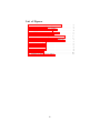
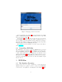
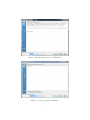
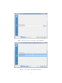
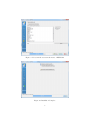
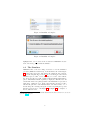
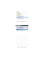
DISPAS v.0.9 - User manual
Cesar Augusto Nieto Coria
Luca Tesei
School of Advanced Studies - Computer Science Department
University of Camerino
2nd September 2014,
Camerino - Italy
Abstract
The present document is an user manual and installing guide for DISPAS. It is going to explain how to install it, as well as the uninstall process.
Further, how to simulate with the tool.
Because of the simulator is fully developed under Java, the process
for installing is the same for all the Operative Systems available on the
market. In the first section we have an introduction to introduce to the
reader on the research context. In the second section is going to explain
how to install and uninstall the simulator. The third section is about the
simulator, their parameters and settings that user may tune with the aim
to test different simulation scenarios.
1
Contents
1 Introduction
1
2 Installation Guide
2.1 Installing DISPASim . . . . . . . . . . . . . . . . . . . . . .
2.2 Uninstalling DISPASim . . . . . . . . . . . . . . . . . . . .
3
3
4
3 DISPASim
3.1 The Simulator Execution . . . . .
3.2 The Simulator . . . . . . . . . . . .
3.2.1 The Simulation Parameters
3.3 A Simulation Execution . . . . . .
I
.
.
.
.
.
.
.
.
.
.
.
.
.
.
.
.
.
.
.
.
.
.
.
.
.
.
.
.
.
.
.
.
.
.
.
.
.
.
.
.
.
.
.
.
.
.
.
.
.
.
.
.
4
. 4
. 8
. 10
. 11
List of Figures
1
2
3
4
5
6
7
8
9
10
11
12
13
14
15
16
17
The von Bertalanffy growth equation chart. . .
DISPASim version 0.9 . . . . . . . . . . . . . . .
DISPASim Installer location example . . . . . . .
Language selection screen-shot . . . . . . . . . .
Brief information page about DISPASim . . . . .
License agreement of DISPASim . . . . . . . . .
Selection of the location path for the installation
Screen-shot of the installation finished . . . . . .
Selection if the user want shortcuts of DISPASim
Installation Complete . . . . . . . . . . . . . . .
Installation Complete . . . . . . . . . . . . . . .
Installation Complete . . . . . . . . . . . . . . .
DISPASim Directory . . . . . . . . . . . . . . . .
DISPASim Directory . . . . . . . . . . . . . . . .
2D view example . . . . . . . . . . . . . . . . . .
3D view example . . . . . . . . . . . . . . . . . .
Simulation parameters screen-shot . . . . . . . .
II
.
.
.
.
.
.
.
.
.
.
.
.
.
.
.
.
.
.
.
.
.
.
.
.
.
.
.
.
.
.
.
.
.
.
.
.
.
.
.
.
.
.
.
.
.
.
.
.
.
.
.
.
.
.
.
.
.
.
.
.
.
.
.
.
.
.
.
.
.
.
.
.
.
.
.
.
.
.
.
.
.
.
.
.
.
. 2
. 2
. 3
. 4
. 5
. 5
. 6
. 6
. 7
. 7
. 8
. 8
. 9
. 9
. 9
. 10
. 11
1
Introduction
Overfishing in the Mediterranean Sea has gained an increasing consideration in the last years. In particular, the potential damages in the recovery
capacity of the commercial stocks. Besides a lossy controlled fishing activity could be a serious problem if it is not faced with appropriate information and scientific support. With this aim the Demersal fIshing Stock
Probabilistic Agent based Simulator (DISPAS ) was developed. With it
is possible to gaining a better understanding of the marine exploitation,
performing the stock assessment. Particularly, this simulator was developed for a living species in the Adriatic Sea, the common solea Solea solea
(Linnaeus, 1758; Soleidae). Witch main fish population is concentrated
in the north and central part of the Adriatic Sea.
DISPAS has been developed following the Agent Based Methodology,
that is a growing approach with an increasing number of applications.
Scenarios where this methodology can be applied are from different and diverse contexts like ecosystem environment, chemical reaction simulations,
financial markets simulations, decisions support systems, traffic control
systems. With regards to the purpose of the simulator, e.g. simulating
the marine ecosystem in the Adriatic Sea, we need modeling techniques
that can deal with the complexity of the task. This led to the use of the
agent-based methodology for developing DISPAS.
The simulator is able to reproduce a good number of scenarios, for
example generating a random population or from a text file. Also, allows
the user to change parameters for the simulation interactively within the
Repast Symphony framework. The simulated space represents a square
km of the Adriatic Sea. It is displayed by a grill of hundred meters per
hundred meters (100m x 100m) in which the individuals, our specie of
study: common soles, are living. The current view is in two dimensions
(2D), but the simulator also has the capability to display a 3D view, were
the agent size and the difference between the different age classes can
be appreciate. As it was mentioned the individuals are classified in an
age classes division. It is performed applying the von Bertalanffy growth
equation, which is the most widely used growth curve and is specially
important in fisheries studies.
The principal objective of the simulator is the common sole stock assessment. In order to accomplish it DISPAS uses input data coming from
the SoleMon project, which is based on an independent fishery study, collecting data directly from independent surveys in the Adriatic Sea. For
this work we have been provided with the data from the National Council
of Research (CNR). We used data that is the number of soles per each
age class found in the same square km every year in November from 2005
to 2011. After processing the data, we have derived the fishing probability and the natural mortality probability for soles, divided into five age
classes. We obtain the probabilities and quantities monthly for each agent
age classes.
It was mentioned above, the agents are classified in five age classes,
the classification is made using the von Bertalanffy growth equation. The
simulator calculates sole’s length in function of its age, in a particular
time using the von Bertanlanffy growth equation.
1
Figure 1: The von Bertalanffy growth equation chart.
Figure 2: DISPASim version 0.9
The time is an important characteristic, because it provides the individual’s notion of evolution. In DISPAS at each time step (tick, in Repast
Simphony) represents a month of the year. The simulator uses the data
derived by the SoleMon Project, that it consist in scientific independent
surveys, as input. The data encompass the fish quantity belonging to each
fish classes as well as the indexes for the natural mortality probability and
fishing probability. After execute the simulation, DISPAS saves in an external text file the results of simulation, with the following information:
Total Biomass and Number of individuals per Class.
2
Figure 3: DISPASim Installer location example
2
2.1
Installation Guide
Installing DISPASim
The starting point of this guide is download the DISPAS installation package that can be found in the following Link. DISPAS was developed using
the Repast Simphony (RS) framework, in RS the modeler can develop in
which language he/she prefer, e.g Java, Python, Netlogo, Groovy, etc.
The RS suite runs under Java, it means that to be able to run our model
we need to have installed the Java Virtual Machine, if the computer does
not has it before we need to download and run the next installer, this is
usually for MS Windows users. In the other hand if you are a GNU/Linux
user, is much easier just to open your shell console and download as usually for any program that you have installed before. For e.g in Ubuntu is:
# sudo apt-get install java
Furthermore, in the following Link the user can find the different Java
distribution, in order to download and install it. Once that we have
the JVM and downloaded the installer package we can proceed with the
installation. Go to the place that you have downloaded the installer, in
order to execute you have to make double-click in the DISPAS setup.jar.
As soon as, we have downloaded the installation package, make doubleclick on it, then is going to start the installing process. The installation, is
a regular software installation process (with windows environment). The
DISPAS installer can be executed in all platform. The first screen-shot
(Figure 4) that we have is where the user can select the installing language.
Once that we have choose it, press Ok button.
3
Figure 4: Language selection screen-shot
The next installation step, Figure 5, is a brief information about DISPAS, to continue press the button Next. Following, we have to agree with
the License Agreement (Fig. 6).
In the Figure 7 displays the next step where the user can select the
folder installation location. If the user wants to install it in the root
directory might execute the installation package with the those privileges.
After that, the installation will proceed. And the successive step will as
if the user want to create the DISPASim shortcuts.
The installation is pretty intuitive, if you have any problem with it,
please contact us.
2.2
Uninstalling DISPASim
The uninstall process is going to delete the DISPASim from your hard
disk, as is displayed in the Figure 11, the highlighted folder in the where
is it the Uninstaller package. In order to execute it, the user just have
to make double-click in it. So, the uninstall process will start, as it is
displayed in the Figure 12 Finally, when it is complete the user can close
the window. Note, after the uninstallation some directories are going to
remain in your installation location, those are where the simulator output
files were stored.
3
3.1
DISPASim
The Simulator Execution
In the section below we are going to explain how to execute and tune the
simulator. First, we are going to see how to execute; in your DISPASim
location folder, you might have something like in the Figure 13. The
4
Figure 5: Brief information page about DISPASim
Figure 6: License agreement of DISPASim
5
Figure 7: Selection of the location path for the installation
Figure 8: Screen-shot of the installation finished
6
Figure 9: Selection if the user want shortcuts of DISPASim
Figure 10: Installation Complete
7
Figure 11: Installation Complete
Figure 12: Installation Complete
highlighted file, start model.bat is the executable for DISPASim. Doubleclick on it and is going to lunch the simulator
3.2
The Simulator
DISPASim allow to the user change Parameters before the simulation
gets start (Simulation Parameters) on the RS framework. In the Figure
14 is showed the upper part of the framework, with it the user can start,
stop, restart and pause the execution1 . Above was mentioned, the current
simulation space is a km2 of area, intending to be a km2 of the Adriatic
Sea. It is represented by a grill of 100m x 100m in with the individuals are
placed. The simulator has the capability to display two different views: 2D
and 3D. The 2D view is a plain grid where the individuals are represented
with circles of different colors. In the other hand the 3D view is a three
dimensional grid where each individual has it own characteristics, one of
it is the shape size. It changes along the execution depending the age class
that the agent belongs to. The Figure 15 and Figure 16 are examples of
the two different views.
1 The user may not be familiarized with the RS framework, then for know more about can
open this Link, Page 23
8
Figure 13: DISPASim Directory
Figure 14: DISPASim Directory
Figure 15: 2D view example
9
Figure 16: 3D view example
3.2.1
The Simulation Parameters
In this subsection we are going to explain the simulation parameters, a
screen-shot is the following Figure 17
• Default random seed: is given from the RandomHelper class that
belongs to RS, it is the seed that is generated randomly by the
compile, to work with pseudo-random numbers.
• Is virgin stock: Is a boolean variable where the user might decide
the nature of the initial stock, it means that if the user decide to
put a period where the mortality probability by fishery, it is equal
to zero. Hence, the agents dies by the natural mortality probability.
• Is the number of newborn variable. It was a boolean value by default
value is false. It means if we checked the box we want to simulate a
random stock value from the tick zero. Otherwise (unchecked state)
the simulator is going to take the initial values from the survey file.
• Survey data file path: The file path where is the survey data (real
data). Default: /Dispas/misc/input FISHPASS.csv (it should not
be changed). Or here you place your own file data input.
• World Height: Default value 100 ms.
• World Weight: Default value 100 ms.
As the user wish, the world size could be changed, making variety
values of the [Height,Weight] making it of the desirable size, but for
our purpose we are going to take as a default value the [100,100].
• L inf (Max fish length): 39,6 cm is the default value.
• A Factor (length/weight): Default Value: 0,007.
• B Factor (length/weight): Default Value: 3,0638.
• kVB (length grow rate): Default Value: 0,44
• t 0 VB: Default Value: -0,46.
10
Figure 17: Simulation parameters screen-shot
Besides, in DISPAS we are going to study the growth rate of our
population. In order to performe this study we were using the von
Bertalanffy growth function where the body length is a function of
age. This four parameters are outcome from the SoleMon project
and default value for this L inf, A, B, kVB, t 0
3.3
A Simulation Execution
At the first time when the start button is pressed, the class context builder
is lunched, this activity triggers a series of action that are going to be
described as following:
• In the previous explanation we saw all the parameters that the user
could change for each simulation. Firstly the simulator allocates
each agent in a random position in our simulated world, as we saw
each agent in the 2D world is represented by a circle of different
colors. It’s given by the agent age class bellowing, from class 0 to
class 5 then we can see the list of colors:
Color Red: Agent class 0
Color Blue: Agent class 1
Color Green: Agent class 2
Color Cyan: Agent class 3
Color Orange: Agent class 4
Color Black: Agent class 5
The user should remember that fish class (agent age class) depends
on the length and growth. It means that meanwhile the time is
passing, the individuals are evolving, this evolution is reflexed in the
agent age class change.
11
• The quantity of the initial stock could comes from two different
sources. One that we should decide initialize our virgin stock in a
random way (Is virgin stock equals true). The second one is taken
the data from our own survey file.
• When the user press the play button the simulation is going to start,
is essential remember that in the temporal aspect RS tool kit use
the sense of tick (a single tick could take any representation that we
would want hours, minutes, seconds, milliseconds and so on) in our
simulator each tick is equivalent of a month, for example in the tick
number 1230 and taken as point of start the 2.005 year we are in
June of 2.107 year.
• The newborns agents are added respecting the amount indicated on
the survey file, in the current version of the simulator the newborns
are added in June of each year. Due to a biological conditions of
the common sole. However, where are not more data available, the
newborns are added in a random quantity, depending on the last
year data, and making it change depending on a calculated standard
deviation.
• Finally, the simulated population generated with DISPASim is stored
in an external text file, in the following address: /Dispas/output
Note: The current document is not the final version of the user manual,
but is pretty accurate with the first version. In case of the user has any
question not doubts to contact to the authors.
12