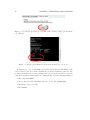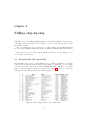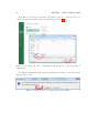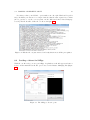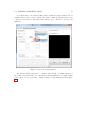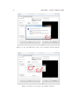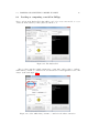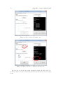
1
Prepared under the PROSIL project by: Dario Cattaneo, Alessio Mauro Franchi and
Giuseppina Gini
SARpy - User’s Manual
2015, April 27th
SARpy - User’s manual
c COPYRIGHT 2015 by Dario Cattaneo, Alessio Mauro Franchi and Giuseppina Gini as
part of the PROSIL project.
If you intend to use the SARpy tool please cite:
Ferrari, T. and Cattaneo, D. and Gini, G. and Golbamaki Bakhtyari, N, and Manganaro,
A. and Benfenati, E. ”Automatic knowledge extraction from chemical structures:
the case of mutagenicity prediction”, SAR and QSAR in Environmental Research,
Volume 24, Issue 5 pp. 365-383 — DOI: 10.1080/1062936X.2013.773376
ALL RIGHTS RESERVED
Contents
Introduction
i
1 Prerequisites
1
2 Installing and starting SARpy
3
3 Working with datasets
3.1 Loading a dataset . . . . . . . . . . . . . . . . . . . . . . . . . . . . . . . . .
3.2 Managing the current dataset . . . . . . . . . . . . . . . . . . . . . . . . . .
5
6
7
4 Working with rulesets
4.1 Creating a model with SARpy . . . . . . . . . . . . . . . . . . . . . . . . . .
9
10
5 Predicting and validating
13
6 SARpy step-by-step
6.1 Preparing the CSV dataset file .
6.2 Loading a dataset in SARpy . . .
6.3 Loading or computing a model in
6.4 Predicting and validating . . . .
. . . . .
. . . . .
SARpy
. . . . .
.
.
.
.
.
.
.
.
.
.
.
.
.
.
.
.
.
.
.
.
.
.
.
.
.
.
.
.
.
.
.
.
.
.
.
.
.
.
.
.
.
.
.
.
.
.
.
.
.
.
.
.
.
.
.
.
.
.
.
.
.
.
.
.
.
.
.
.
.
.
.
.
.
.
.
.
17
17
19
25
29
Introduction
Welcome to the SARpy user guide; this brief manual will introduce you to the SARpy tool,
providing you with the basic knowledge for using this software. An illustrated step-by-step
example is also provided in the last section.
SARpy is an easy tool suitable for building SAR models for regulatory and other purposes. The tool provides the capability to create a personalized model for a specific endpoint, obtaining then a tailored ruleset from the chemical and property dataset. Furthermore you can use this generated ruleset for making predictions about the activity of other
unseen compounds. SARpy is useful also for model validation; with this tool it is easy
to separate the starting dataset into a training and a testing set. A set of rules can be
computed from the former, while the latter can be used for validation of the model.
Before starting, please check the prerequisites section and make sure your computer is
compatible with SARpy. Briefly, the second section will guide you during the installation
process; in the third and fourth you will work with dataset and ruleset respectively; the
last one will explain you how to predict and validate the model.
If you intend to use the SARpy tool please cite:
Ferrari, T. and Cattaneo, D. and Gini, G. and Golbamaki Bakhtyari, N, and Manganaro,
A. and Benfenati, E. ”Automatic knowledge extraction from chemical structures:
the case of mutagenicity prediction”, SAR and QSAR in Environmental Research,
Volume 24, Issue 5 pp. 365-383 — DOI: 10.1080/1062936X.2013.773376
i
Chapter 1
Prerequisites
The software and hardware prerequisites for installing and using SARpy tools are as follows:
• Microsoft Windows XP SP1\SP2\SP3, Vista, Windows 7, or Windows 8;
• Any Intel or AMD processor x86 or x64 (suggested Intel Core i5-750 or greater);
• 512MB RAM (1GB or more for huge dataset);
• Up to 100MB available hard disk space (dataset files not included);
• Administrator rights are not needed for the installation process but suggested;
• A compression\decompression software (Windows built-in tool, WinZip, WinRar).
It is a recommended best practice to back-up your system and data before you remove
or install software.
1
Chapter 2
Installing and starting SARpy
The SARpy tool is distributed as a .ZIP package; this archive contains all the files the tool
needs to work correctly. Once you have downloaded the package from the download area
of the VEGA website (SARpy link), simply unpack it in any folder you like. To extract
the files you can use the Windows integrated ZIP tool, or any file compression software you
prefer (e.g. WinZip or WinRar).
Now enter in the folder just created and double click on the file ”SARpy.exe”; the
software will automatically starts showing its splash screen for a few seconds. After that
the main window should appear, focused on the Dataset Managing Tab, as shown in 2.1.
Figure 2.1: The main window of the SARpy tool.
3
Chapter 3
Working with datasets
SARpy’s Dataset Managing Tab allows the user to work with datasets; the general appearance of this tab is shown 3.1. With the word dataset we mean ...
By this tab it is possible load and manage a dataset, either for using it as training set to
generate models, or as test set to validate models, or as a collection of untested molecules
whose activity has to be predicted.
Figure 3.1: The figure shows the Dataset Managing Tab; here you can load and customize
a dataset.
.
Basically, SARpy Dataset Managing Tab allows the user to perform two main actions:
• Loading a new dataset from external files (see section 3.1);
• Managing and preparing the current dataset (see section 3.2).
5
6
CHAPTER 3. WORKING WITH DATASETS
3.1
Loading a dataset
SARpy is able to read only a specific dataset format based on SMILES, which is automatically created by the system itself using data coming from externals sources such as
text or excel files. All molecular structures contained within the selected external file are
read, parsed and converted in the specific SARpy format, and then memorized as a SARpy
dataset. This method assures the reliability of the dataset and a short elaboration time.
SARpy accepts as external data source only files saved with either the .CSV or .SDF
extension. Please be sure your file meets correctly the format specification:
• CSV format: all the floating values must use the dot as decimal separator; as the
CSV file requires each value must be separated by comma; the file must be columnwise (i.e. each column is a property); the first row of the file must contain property
labels;
• SDF format: all the floating values must use the dot as decimal separator; each
entry must be separated by the character sequence ”$$$$”; each property name must
be surrounded by ”><” and ”>” .
To load the external file simply select its format and then click on ”Browse” (Figure
3.2); to check if the operation was successful check whether all the other functionalities in
this tab are now available or not.
Figure 3.2: How to load an external file: first select the file format and then browse for it
on your computer
.
3.2. MANAGING THE CURRENT DATASET
3.2
7
Managing the current dataset
Once the set of molecules has been correctly loaded from external file, you may manage
the loaded data according to your own needs; once you do that, simply click on the ”Load”
button in the bottom of this tab so that SARpy can create its own internal dataset. If it
has been correctly created, the filename of the external data source and the total structure
count should be reported on the right, just above the ”Info Dialog” (Figures 3.3 and 3.4.
Figure 3.3: Once you are ready with your
dataset, just click on the ”Load” button
you find in the bottom of this tab.
Figure 3.4: The image show the Info
Panel, useful to check for error on every
load operation.
.
Basically, user can manage the current dataset in two ways:
• Binarizing the current dataset (see section 3.2);
• Filtering the current dataset (see section 3.2).
Binarize a dataset
Even if SARpy may properly work using a non-binary classification (i.e. considering more
than two activity classes), a lot of case studies usually divide the compounds using a binary classification scheme, generally labeling each compound with the generic ”Active” or
”Inactive” labels. The binarization tool provides you with the capability to create this kind
of classification from a multi-class one, relabeling the classes. The binarization operation
requires you to specify which of the present classes are to be considered as active and which
are instead considered as the inactive ones. Once the binarization operation is done, all
molecular structures will change their activity description according to the new parameters;
all the previous information regarding the previous activity labeling are not lost and are
retrievable simply by unchecking the ”Binarize” checkbox.
The binarize tool also works with datasets that use continuous values; in this case a
proper threshold value within the range must be specified in order to split the set into
”Active” and ”Inactive” molecules. Please refer to the 6 in order to learn more about this
functionality.
Filter a dataset
A second important tool provided in SARpy is for filtering data. Testing methodologies
often need to split a datasets into several subsets, each with a particular property: a classical
example is the division in training and testing sets, the first dedicated to the generation of
the model, the second used only for validating the model. This constraint tool allows the
user to apply one or more constraints on the whole dataset, splitting it into several parts,
and obtaining a reduced dataset that meet the given restrictions.
8
CHAPTER 3. WORKING WITH DATASETS
Figure 3.5: To binarize a dataset check the highlighted checkbox and move all the labels in
the right new class.
Figure 3.6: Here is the filtering tool; select the property you need to filter by and compose
the filtering rule.
Chapter 4
Working with rulesets
SARpy’s Ruleset Managing Tab allows the user to create a SARpy ruleset, that is a list of
rules that establishes relationships among various substructures and the selected activity
classes. These rules are written using the SMILES format for the chemical structures, and
always follow this syntax:
CC(C(= O)O)c1ccccc1
Developmental toxicant
1.06
(4.1)
This syntax indicates that the selected fragment usually identifies the activity of a
molecule as Developmental toxicant, with a likelihood ratio of 1.06. SARpy’s rulesets are
therefore models for molecular activity, and so they must be generated taking into account
a wide range of conditions that allow users to improve the overall reliability of each model
to the specific target’s characteristics. The general appearance of Ruleset Managing Tab is
shown in Figure 4.1.
Figure 4.1: The Ruleset Managing Tab.
9
10
CHAPTER 4. WORKING WITH RULESETS
Unlike the datasets, that are only loaded onto the system starting from an external
file, a ruleset (i.e. a model) might be saved to be loaded again after in order to analyze
molecules on the same endpoint. These models are saved by SARpy in a user specified
folder, in plain TXT text format, and are then easily interpretable and ready-to-use for
scientific publications and papers.
To load or save a ruleset, the user must use the dedicated buttons and follow the
instruction on the dialog window that will open. Otherwise, to create a brand new model
the user must have a dataset loaded and have to specify several parameters to extract
meaningful rules. The loaded dataset must be valid and must contain at least two activity
classes: if it is not the case, most of all the options are disabled.
4.1
Creating a model with SARpy
SARpy has two ways of creating models; these are similar in the produced result and in the
way they operate, but generate models that have different purposes. You can use SARpy
as:
• A classifier to predict a property: SARpy will generate a model that establishes
relationships between each found substructure and all the activity classes specified
during the dataset loading operation. Models generated with this modality consist of
a list of rules that might be used to classify other molecules into one of the considered
classes. Since the purpose is to predict the activity of new structures, rules generated
in this modality are generally more detailed than rules produced in the Extractor
mode.
• A knowledge extractor tool to extract relevant substructures: the SARpy tool tries to
generate some new knowledge from the current dataset, analyzing it versus a singular
activity class, and establishing relationships among substructures and the specified
activity class. This modality produces a list that is somewhat less specific than the
one produced in the other mode, but gives sound information about substructures
that are possibly related to a specific activity.
Generally speaking, each SAR model works better for molecules that have similar characteristics; this means that SAR models might always be tailored around the specific batch
of structures being used to create it. So, a minute regulation of a certain number of parameters is generally possible for SAR model generation. SARpy is not an exception, as
it provides some functionalities that affects robustness, sensitivity and sensibility of the
developed models.
Through the user interface the user can regulate models precision and the definition of
the structural alerts themselves.
4.1. CREATING A MODEL WITH SARPY
11
• Model precision: SAs extracted by SARpy are usually associated with numbers
that defines their precision; the user can regulate the level of sensitivity and specificity by various parameters that affect the alert precision. For a quick tuning there is
an ”Auto” setting, by which user has just to select among three predefined values of
precision: ”min” means a more ”sensitive” result (i.e. it minimizes the unpredicted
rate) while ”max” will produce a more ”specific” result (i.e. it minimizes the error
rate). In alternative, using the ”Manual” regulation mode the user can set the minimum likelihood ratio he prefer for each structural alert. An increase in this parameter
corresponds to a higher precision of the model.
Figure 4.2: From this panel it is possible to regulate the precision of the model to be
generated.
• Structural Alerts Options: the process of creating a new model implies the analysis of each molecular structure and the fragmentation of molecules into several substructures; these last are are matched with the information about activity in order
to establish any possible relationship between substructures (i.e. structural alerts,
SAs) and activities. SARpy gives the user the capability to define some parameters
of the SAs: the maximum and the minimum number of atoms each SA is composed
of (which affect the number of SAs considered and the computation time) and the
minimum number of occurrences needed for each SA to be considered as valid (higher
values correspond to more precision).
Figure 4.3: After you have checked the ”Structural Alerts Options” , it is possible to modify
parameters regarding the structure of the SAs.
12
CHAPTER 4. WORKING WITH RULESETS
After every parameters is set up correctly, just click on the button ”Extract and Validate” to generate the model; the info panel will show you the progress of the computation.
Figure 4.4: Once every desired properties of the model have been set, click on the ”Extract
and Validate” button to generate the model.
Chapter 5
Predicting and validating
This last section of the SARpy tool is the Prediction and Validation Tab; once you have
correctly loaded a dataset in the system and created or loaded a set of rules (as seen in
the two previous sections), through this tab you can predict the activity of other unseen
compound (i.e. apply the ruleset on the dataset) and also validate the model.
Here is represented this tab (Figure 5.1).
Figure 5.1: The Predict and Validate Tab.
To predict the activity of the compounds listed in the testing dataset you simply have
to click on the ”Predict” button you find in the top of this tab. The process will be quite
fast and you can check whether it has finished reading the info panel on the right: when
the process is over you should read ”xxx structured matched”, as shown in figure 5.3.
13
14
CHAPTER 5. PREDICTING AND VALIDATING
Figure 5.2: To start the prediction process click on the ”Predict” button you find in the
top of this tab.
Figure 5.3: The info panel will show you when the prediction process is over.
Now that the process correctly finished you can save the prediction result clicking on the
”Save prediction” button; a text file containing the prediction result will be generated. The
prediction information are row-wise, meaning that each row is the prediction of a specific
compound found in the dataset. Each row contains, in this order, the following information:
• The compound SMILE;
• The prediction as a label (standard values are ”Active and ”INACTIVE”);
• The likelihood-ratio test value;
• The SMART.
15
Optionally it is possible to add in this output other information among those contained
in the dataset; to do this just select those you want to add from the list before saving the
prediction result (see figure 5.4).
Figure 5.4: Select from this list all the attributes you would like to add to the prediction
result.
The last step you can perform is model validation, that will give you information about
the model performance and will check the accuracy of the model’s representation of the real
system. To start the validation of the generated model on the loaded dataset just click on
”Validate” button you find in the middle of this tab; as the process finish, the info panel will
give you the relevant information (i.e. the error rate and the confusion matrix) regarding
the model performance (see figure 5.6).
Figure 5.5: Click on the validate button to start the model validation process.
Figure 5.6: As the validation process is over the info panel will show its result.
Chapter 6
SARpy step-by-step
This last section of the SARpy manual will guide you through the SARpy tool step-by-step,
performing each action needed to load a dataset, to create or load a ruleset and to predict
and validate a result.
The toy example here proposed is based on a public dataset from the Environmental
Protection Agency (EPA), Mid-Continent Ecology Division, Duluth (MN). This dataset is
...
Important note for user: this is only an example about how to use the SARpy tool; we
do not want to buid a model.
6.1
Preparing the CSV dataset file
The first thing you need before opening SARpy is a .csv or .sdf file containing the compounds
dataset. Here we will start from an .xls file; the file must be column-wise, i.e. each column
represents a property you have in the dataset (SMILE, Name, ID, class and so on) and the
first row of the file must specify the property label (see figure 6.1). Please note also that
floating point value must use the dot as decimal separator.
Figure 6.1: The example dataset loaded as Excel file.
17
18
CHAPTER 6. SARPY STEP-BY-STEP
From Excel you can export a CSV file: just click on ”Save as...” and select the .cvs
extension from the list available under the file name (see figure 6.2)
Figure 6.2: To export your .xls to .csv simply save the file and choose the .cvs extension
from the list.
It can happen that an information message stating that you will loose some file features
appears; click on ”Yes”.
Figure 6.3: Click on ”Yes” to close the message and continue.
6.2. LOADING A DATASET IN SARPY
19
Now that you have your CSV file, open it with a text editor (the Windows Notepad is
fine); check that your data are not corrupted and also that the value separator is a comma
(if not, you have to set the correct separator in the Windows Control Panel, Language
section). The file should look like the one showed in figure 6.4.
Figure 6.4: Edit the file .csv just extracted and verify that it meets all the prerequisites.
6.2
Loading a dataset in SARpy
With the .csv file ready you can open SARpy. A splash screen should appear and after a
few second the main window should open, focused on the Dataset Managing Tab (Figure
6.5).
Figure 6.5: The SARpy tools as it opens.
20
CHAPTER 6. SARPY STEP-BY-STEP
The first thing you have to do is to load the .csv external file, only after having selectend
the file format you are about to use; in this example we select ”.csv”. Click then the
”Browse” button to search for the file in your computer (figure 6.6).
Figure 6.6: Look for the .csv file and click on load; if you cannot find it make sure the file
format filter is set correctly.
Now choose from the first dropdown list the SMILES attribute, so that SARpy knows
which column contains the compounds SMILE (6.7).
Figure 6.7: From the list select the attributes for SMILES.
6.2. LOADING A DATASET IN SARPY
21
Secondly, indicate to the software which column contains the activity attribute. In our
example dataset we have added a column called ”Name”, which specifies the class for each
compound. Our classes are just string values, namely ”Low”, ”Moderate”, ”Strong” and
”Extreme”.
Figure 6.8: Select the activity attribute.
The activity attributes may also be a numeric value; in this case SARpy will let you
know that you probably want to set a threshold for binary classification of compund. Click
”Ok” button; a new pop-up will be displayed asking you this numeric threshold (figure
6.10).
22
CHAPTER 6. SARPY STEP-BY-STEP
Figure 6.9: A popup will warn you if you select a numeric activity attribute.
Figure 6.10: In the next popup set the numeric threshold.
6.2. LOADING A DATASET IN SARPY
23
Now you can, let’s say, binarize your dataset; this step is totally optional. By binarize
we mean dividing all the compound in the dataset in two classes, ”Active” and ”Inactive”,
based on the mapping you specify in the three lists.
In our case, as we want the ”Low” and ”Moderate” class to become the ”Inactive”
one, and the two others to represent the ”Active” class, we simply move the four labels
respectively in the right or in the left list (see figure 6.11).
The same happens with a numeric threshold: you will have to decide whether the bigger
or the lower values of the threshold defined above are to be set in the ”Active” on ”Inactive”
class.
Figure 6.11: Use the arrow to move the class on the ”Active” or ”Inactive” side.
The last step you can perform is filtering the dataset, i.e. selecting only some specific
entries and discarding all the other not meeting the property specified. In the example we
want to throw away all the molecules with an ID number greater than 200 (figure 6.12).
24
CHAPTER 6. SARPY STEP-BY-STEP
Figure 6.12: Check the ”Filtering” option if you want to discard some dataset entries.
Now that every parameter is set up, it is time to load the dataset in SARpy, simply
clicking on the ”Load” button. Read the info panel on the right to check how many
molecular structure have been loaded and check on top of this if the file name is correct
(figure 6.13).
Figure 6.13: Last click on ”Load” button to start the dataset creation process.
6.3. LOADING OR COMPUTING A MODEL IN SARPY
6.3
25
Loading or computing a model in SARpy
The second tab is the Ruleset Tab, that will let you load or create a new model, i.e. a set
of rules, from the dataset you have just loaded in the tool.
Figure 6.14: The Ruleset Tab.
Here you have just three simple parameters to setup; first of all you have to indicate
which classes you want to consider for model extraction; for nomal application select ”All
classes” as shown in figure 6.15.
Figure 6.15: Select which class you want to consider for the ruleset extraction.
26
CHAPTER 6. SARPY STEP-BY-STEP
Now its time to specify the structural alerts options: you can set its minimum and
maximum number of atoms and its number of occurencies to be considered as significant
(the higher this last number is, the less restrictive, but more precise, will be the model.
Default values suggested are two atoms (min) and eighteen atoms (max). Changing
these two numbers affect not only the number of the SA that will be present in the model,
but also has a strong influence on comptation time.
Figure 6.16: Set the values you prefer for structural alerts options
The next parameter of the model is the single alert precision, i.e. the minimum likelihood
required by the model. This value affect its precision and accuracy; there are two main
options, ”Auto” (on the left) or ”Manual” (on the right).
The first let the user select among three predefined values: ”Max” (that will give a
more ”specific” result, minimizing the error rate), ”Min” (for a more ”sensitive” result that
minimize the unpredicted rate) and ”Optimal” (a trade-off between these two).
Otherwise, with the second option you can set the minimum likelihood ratio you like:
increasing this parameter strengthen the precision of the model.
For this example tutorial we selected ”Auto-Max” mode.
6.3. LOADING OR COMPUTING A MODEL IN SARPY
27
Figure 6.17: Set the single alert precision you prefer; a higher LR will result in a higher
precision of the model.
To start the extraction and validation process click on the ”Extract and validate” button
you see in the bottom of this tab. While the process is running check the info panel (see
figure 6.18).
Figure 6.18: Click on ”Extract and validate” to build the model.
28
CHAPTER 6. SARPY STEP-BY-STEP
After some minutes (the computational time can vary depending on the dataset loaded
and on the hardware you have), the model is created; in the info panel its accuracy and
confusion matrix will be displayed.
Figure 6.19: When the process is over the info panel will show some information about the
model.
If you need you can save the resulting model, so that you can load later, maybe with
a different dataset (see figure 6.19). To do this simply click on the ”Save ruleset” button
located on the right of the ”Extract” button and select where you want to store the file, as
shown in figure 6.20.
Figure 6.20: When saving the ruleset make sure the .txt format is selected.
6.4. PREDICTING AND VALIDATING
29
A plain text file will be created. Its structure is quite simple and is shown in figure 6.21:
each row is a rule, and contains the fragment SMART, the training class (as ”Active” or
”Inactive”) and the normalized likelihood ratio.
Figure 6.21: In the image is shown an example of the ruleset file as created by SARpy.
6.4
Predicting and validating
Once you have correctly loaded a dataset and a ruleset, you can switch to the last tab,
the ”Predict and validate” tab; by this tab you can predict the activity of other unseen
compound, i.e. apply the ruleset on the dataset, and also validate the model, i.e. compute
the prediction error and the confusion matrix. This tab is shown in figure 6.22.
To predict the property of each compound in the selected dataset simply click on the first
button, ”Predict”; the info panel will show you how many structures have been matched
(figure 6.23).
30
CHAPTER 6. SARPY STEP-BY-STEP
Figure 6.22: The ”Predicte and validate” tab.
Figure 6.23: Click on ”Predict” to run the prediction process.
If you need it, you can save the prediction results as text file; just click on the ”Save
predictions” button, select the folder and the file name and make sure the selected format
is .txt.
6.4. PREDICTING AND VALIDATING
31
Optionally you can select some attributes of your dataset to be added to the prediction
output. To do this, select those you want from the list; multiple selection is performed by
pressing and holding the shift key while clicking on attributes.
Figure 6.24: How to save the prediction result as text file.
These attributes are in addition to those saved by default. The file produced in this
example is shown in figure 6.25; each compound is listed in a row, with its SMILE, the
predicted class (Active or Inactive), the likelihood ratio and the SMARTS, also with the
LC50 value and the original class of the compound.
Figure 6.25: An example file containing the saved predictions.
32
CHAPTER 6. SARPY STEP-BY-STEP
The last tool you may want to use is the validation, useful to compute the error rate
and the confusion matrix of the model when applied to the loaded dataset (figure 6.26).
Figure 6.26: To validate the model click on the ”Validate” button and read the result in
the info panel.