Download User Manual of FitSuite 1.0.4

User Manual of FitSuite 1.0.4
SAJTI Szilárd
July 18, 2009
U SER M ANUAL OF F IT S UITE 1.0.4
July 18, 2009
S AJTI Szilárd
Contents
1 Introduction, antecedents
1
2 Basic concepts of FitSuite
2.1 Experimental scheme and its structure . . . . . . . . . . . . . . .
2.2 Transformation matrix technique . . . . . . . . . . . . . . . . . .
2.3 Parameter distribution . . . . . . . . . . . . . . . . . . . . . . . .
2.4 Statistics . . . . . . . . . . . . . . . . . . . . . . . . . . . . . . .
2.5 Error estimation, bootstrap method . . . . . . . . . . . . . . . . .
2.6 Fitting . . . . . . . . . . . . . . . . . . . . . . . . . . . . . . . .
2.6.1 Constraints (Simple bounds) . . . . . . . . . . . . . . . .
2.6.2 Distributed parameters (using maximum entropy principle)
2.6.3 Rescaling parameters . . . . . . . . . . . . . . . . . . . .
2.6.4 Numerical derivatives . . . . . . . . . . . . . . . . . . .
2.7 Subspectrum . . . . . . . . . . . . . . . . . . . . . . . . . . . .
2
2
3
6
7
11
14
15
17
18
18
20
3 Working with FitSuite
3.1 Starting a new project . . . . . .
3.2 Building up the model structure
3.3 Adding data . . . . . . . . . . .
3.4 Changing parameters, matrices .
3.5 Report generator . . . . . . . .
3.6 Cloning . . . . . . . . . . . . .
3.7 Model groups . . . . . . . . . .
3.8 Simulation, Fit . . . . . . . . .
3.9 Error calculation . . . . . . . .
3.10 Calculating statistics . . . . . .
3.11 Plotting . . . . . . . . . . . . .
3.12 Sounds . . . . . . . . . . . . . .
3.13 Examples . . . . . . . . . . . .
20
21
22
23
24
26
27
27
28
31
31
31
32
33
.
.
.
.
.
.
.
.
.
.
.
.
.
.
.
.
.
.
.
.
.
.
.
.
.
.
.
.
.
.
.
.
.
.
.
.
.
.
.
.
.
.
.
.
.
.
.
.
.
.
.
.
.
.
.
.
.
.
.
.
.
.
.
.
.
.
.
.
.
.
.
.
.
.
.
.
.
.
.
.
.
.
.
.
.
.
.
.
.
.
.
.
.
.
.
.
.
.
.
.
.
.
.
.
.
.
.
.
.
.
.
.
.
.
.
.
.
.
.
.
.
.
.
.
.
.
.
.
.
.
.
.
.
.
.
.
.
.
.
.
.
.
.
.
.
.
.
.
.
.
.
.
.
.
.
.
.
.
.
.
.
.
.
.
.
.
.
.
.
.
.
.
.
.
.
.
.
.
.
.
.
.
.
.
.
.
.
.
.
.
.
.
.
.
.
.
.
.
.
.
.
.
.
.
.
.
.
.
.
.
.
.
.
.
.
.
.
.
.
.
.
.
.
.
.
.
.
.
.
.
.
.
.
.
4 Sources, documentation
34
5 To do
34
6 ‘Installation’
6.1 Linux . . . . . . . . . . . . . . . . . . . . . . . . . . . . . . . .
6.2 Windows . . . . . . . . . . . . . . . . . . . . . . . . . . . . . .
36
36
36
7 License
36
I
U SER M ANUAL OF F IT S UITE 1.0.4
July 18, 2009
S AJTI Szilárd
References
38
Glossary
41
Index
45
II
U SER M ANUAL OF F IT S UITE 1.0.4
July 18, 2009
S AJTI Szilárd
1 Introduction, antecedents
FitSuite is an environment for simultaneous fitting and/or simulation of experimental data of vector-scalar type, such as parametric curves and surfaces typically
collected in a physics experiment. Simultaneous here means that several sets of the
same type of experiment and even of different types of experiments can be simulated/fitted in a self-consistent, statistically correct framework with provisions for
cross-correlation of the theoretical and specimen parameters.
Experiments often provide raw data of measurements performed on the same
sample by different methods, and/or using different experimental conditions, like
temperature, pressure, magnetic field, and the like. Data often partly depend on
the same set of experimental and sample parameters therefore a simultaneous evaluation of all experimental data is prerequisite. However, data evaluation programs
are dominantly organized around a single method therefore a simultaneous access
to the data for a common fitting algorithm is not typical. Lacking suitable programs, some parameters are determined from one measurement, assumed errorfree and kept constant when evaluating other experiments, an obviously incorrect approach. Besides, for different methods different programs are used, which
makes it very difficult to tune parameters of such theories and their errors and correlations to each other and to extend or modify the theories to describe different
experimental data.
Therefore, starting in 2004 (as part of the Dynasync FP6 project sponsored by
the European Commission, and since 2006, within the NAP_VENEUS project,
sponsored by the Hungarian National Office for Research and Technology) we
developed FitSuite for Windows and Linux, a code that consistently handles by
now data of over ten spectroscopic methods with over twenty theories together
with a large number of sample structures in a common inter-related framework.
FitSuite is an environment, in which, besides the possibility of adding brand
new (user written) ‘theories’, the user can ‘build’ new theories based on the combination of existing ones, subroutines, which call each other. To our opinion,
this feature of FitSuite is really essential, since a complex physical system can in
general be divided into subsystems and even this subsystem can be divided into
further subsystems, groups of which can be described with the same parameters
and physical equations. To provide an example, assume we have a thin film built
up from layers and the layers may be built up from further object (depending on
to what physical characteristics the method in question is sensitive to) such as
domains, atomic groups, lattice sites, molecules, etc. (E.g. in Mössbauer-related
problems each layer may contain several sites, with their own hyperfine ‘theories’
to calculate the corresponding subspectra).
The original idea of cross-correlation and of hierarchy of theories as well as
a number of subroutines of FitSuite were inherited from EFFI (Environment For
1
U SER M ANUAL OF F IT S UITE 1.0.4
July 18, 2009
S AJTI Szilárd
FItting) [1], an originally Mössbauer spectroscopy-related Fortran program developed over the years by Prof. Hartmut Spiering from University of Mainz. In
view of the friendly and fruitful collaboration between the Budapest and Mainz
groups over the last decades, Prof. Spiering kindly agreed to build in the theories written by him and tested within EFFI into FitSuite in order to promote both
projects. Enlightening discussions with him greatly promoted the FitSuite project.
Although in the last three years the two projects developed in different directions,
we are very grateful for Prof. Spiering’s essential contribution to FitSuite.
In the following, we go through the basic concepts used by FitSuite first.
Thereafter we give a short description of the GUI (Graphical User Interface), how
FitSuite should be used from start to fit and present shortly some examples which
can be found in the directory examples.
2 Basic concepts of FitSuite
In this section, we try to make the reader acquainted with the basic concepts used
in the program, which are necessary to know, in order to be able to use it. Here,
we summarize the principles. The description of the user interface is given in the
next section, there we will see, how these concepts, principles are used in practice.
To be able to simulate (fit), we need to give the program our knowledge of the
problems. In FitSuite we should create simultaneous fit projects first, (which have
file extension *.sfp), which contain the fitting problems consisted of experimental data and of experimental scheme.
2.1 Experimental scheme and its structure
The experimental schemecontains the information necessary for description of
the system consisted of the experimental apparatus(es), about the experimental
method itself and of the system under study (e.g: a measured sample). We know
that the meaning of the word experimental!scheme is a bit different from the
present usage, as it usually contains only the apparatuses, but we did not found a
better one. In our thoughts, we usually separate the apparatus used for observation
and the subject of observation. Here we do not want to do this, as it would lead
a more complex structure, and the experimental scheme selects the characteristic
properties, features of the studied system (and of the apparatus), which are essential to be able to calculate the theoretical pair of the experimental data set, which
is prerequisite for fitting, for checking theory or measurement, etc.
In FitSuite the experimental scheme is built up of objects, which correspond
to physical objects (or concepts) e.g.: source, sample, detector, layer, site, etc. The
experimental scheme is also an object. It has a simple tree structure with one root
2
U SER M ANUAL OF F IT S UITE 1.0.4
July 18, 2009
S AJTI Szilárd
object, the experimental scheme. To these objects belong properties which represent the physical quantities (thickness, roughness, hyperfine field, susceptibility,
EFG, effective thickness, etc.) and some numbers characterizing the experimental
scheme e.g. number of channels, symmetries of the sites, etc.
Besides objects and properties, to each object may belong algorithms for calculation of the characteristic spectra.(In the current built-in problems only the
experimental schemes and the sites have algorithms.) These type of objects are
called model on the program interface, as it is an almost perfect name for them.
This type of structure is needed, because simulating our problem, writing the
simulation algorithms, this structure mirrors the real physical system and therefore
it is a practical, logical choice.
2.2 Transformation matrix technique
In contrast to the last remark of the previous section, the ‘optimization’ methods
used for fitting require a parameter vector and not an object tree structure with
properties. Furthermore in case of simultaneous fitting we usually have the results
of experiments performed in a bit different environment (external field, temperature, etc.) and/or different type of experiments using the same ‘sample’. Therefore
there are a lot of common parameters. To eliminate this type of redundancy and
as it is also convenient for the user to use as few parameters as possible (as it
is more transparent for human and easier to fit in a parameter space with lower
dimension at least if we want to get correct results) transformation matrix technique is used [2]. For this we need also parameter vector (array). Because of these
considerations we have to generate the parameter vector and the initial transformation matrix from the object tree structure mirroring the real physical system.
The model parameters which still contain all the redundancy can be collected in a
vector p = (p1 , p2 , . . . , pn ) , where pi is the vector containing all the parameters
belonging to the i-th model in the current simultaneous fit project. Let denote the
vector of the fitting (or if you like simulation) parameters with P and the transformation matrix with T. The transformation matrix technique uses the expression
p = TP, where dim P ≤ dim p. Above, it was mentioned that this technique is
used in order to eliminate the redundancy arising because of the common parameters, but this is not the unique reason. We can take into account some possible
linear relations between the parameters also, which is a redundancy too.
It is advisable to take into account that there are parameters which according
to expectations will not have interdependencies and therefore the T matrix can
be ‘block diagonalized’. It is more transparent to handle submatrices with lower
dimensions, than one extended sparse matrix. Therefore we have to categorize
the parameters according to our expectation whether the subspace stretched by a
subset of them may have interdependencies or this is very unlikely. (If the user
3
U SER M ANUAL OF F IT S UITE 1.0.4
July 18, 2009
S AJTI Szilárd
finds a case, where our expectations are not met, (s)he is able to unite or split
the submatrices, thus our choice here is not a constraint.) The initial submatrices
generally are identity matrices, but not always. E.g. the thickness of a multilayer
sample will be the sum of the layer thicknesses; in Mössbauer spectroscopy in a
doublet site, the line positions and the measure of the splitting and the isomer shift
will not be independent, etc.
Before going further, we have to mention a few concepts related to this transformation matrix technique used for simultaneous fitting (and simulation). In order to eliminate redundancy arising because common parameters, we often use
the operation
Corr
u∈{j1 ,j2 ,...,js }
: Mn×m −→ Mn×(m−s+1)
(1 6 ji 6 m)
(where Mn×m denotes n by m matrices) defined by
Corr
u∈{j1 ,j2 ,...,js }
T =













T11 . . .
..
.
...
Ti1 . . .
..
.
..
.
T1,jk −1 T1,jk +1 . . .
..
.
Ti,jk −1
..
.
..
.
T1,u−1
..
.
...
Ti,jk +1 . . .
..
.
..
Ti,u−1
..
.
.
Tn1 . . . Tn,jk −1 Tn,jk +1 . . .
Tn,u−1
s
P
r=1
s
P
r=1
s
P
r=1

T1jr
..
.
Tijr
..
.
Tnjr
T1,u+1 . . . 

..
... 
.


Ti,u+1 . . . 


..
.. 
. 
.


Tn,u+1 . . .
(1)
which correlates the parameters belonging to columns j1 , . . . js except of the uth column, which becomes the sum of the s correlated columns. The inverse
of this operation is the decorrelation of parameters. The latter generally is not
unequivocal, of course, therefore user interaction may be needed thereafter, in
order to set the proper fit/simulation parameter values and transformation matrix
elements. We may also split a matrix
µ
¶
ª
©
1 6 iu 6 n
Split : Mn×m −→ M(n−k)×(m−s) , Mk×s
1 6 jv 6 m
{i1 ,i2 ,...,ik }
{j1 ,j2 ,...,js }
4
U SER M ANUAL OF F IT S UITE 1.0.4
July 18, 2009
S AJTI Szilárd
E.g. in case of:



Split 

{1,4}

{2,3,6}
t11
T21
T31
t41
T51
T12
t22
t32
T42
t52
T13
t23
t33
T43
t53

 T21 T24 T25 T27
 T31 T34 T35 T37

T51 T54 T55 T57

t15 T16 t17
T25 t26 T27 

T35 t36 T37 
=
t45 T46 t47 
T55 t56 T57

µ
¶
 , T12 T13 T16
,
T42 T43 T46 
t14
T24
T34
t44
T54

(2)
where the elements denoted by T will correspond to the matrix Mk×s and the elements denoted by T to the matrix M(n−k)×(m−s) . The elements denoted by t will
be eliminated, therefore information will be lost, if they were not 0. Unification
of two matrices can be conceived as the reverse of splitting, but there we set the
cross-elements denoted by t to 0.
Sometimes it is useful to insert a new simulation/fit parameter, this corresponds to insertion of a new column in the transformation matrix. E.g. we know
the value of the sum of some parameters, but we do not know their value. In such
a case we may insert a new parameter, which we keep constant, set it to the value
of the known sum, and set the corresponding matrix elements properly, like here:


 

1 −1 −1 · · · −1
Psum
p1

  P2   p2 
1


 


  P3   p3 
1
(3)


=
.

  ..
  .. 
.
.

 .
  . 
.
1
Pn
pn
Thus we add a constraint for the corresponding parameters and we can eliminate
a redundant fitting parameter and we do not increase the number of fitting parameters, as we would using Lagrange multipliers.
Some parameters are integer numbers (e.g. channel numbers, switches, etc.).
These are never fitted, but the transformation matrix technique is useful for them,
especially if some of them have the same value. The integer and real number based
parameters are separated in the program and on the user interface too, to avoid
the possibility of rounding errors, because of the finite precision of the computer
representation of the numbers. This does not means, that in some cases it would
not be reasonable to mix the number types, but it is safer, than what we could gain
allowing mixing. Everything we said about the transformation matrix for real
parameters is valid for integer parameters, except of the fact, that in this case we
have integer matrix elements, just because of the above mentioned considerations.
5
U SER M ANUAL OF F IT S UITE 1.0.4
July 18, 2009
S AJTI Szilárd
2.3 Parameter distribution
In physics we often have not a single well defined physical object, but rather an
ensemble of them. Even in this case, it may be useful to represent them with a
single object in our (computer) model, but we have to know that which parameters are the same for the members of the ensemble and which are different. We
can group the objects according to these parameters. The parameter distribution
fd (pd ) will give the probability that the ensemble has objects, ©
which
ª can be differd
entiated from other members according to the parameter set pk (which is part
of the set of all the parameters {pi }). As usually this distribution is unknown, we
have to determine it by fitting too. There is no sense in defining the distributions
on the level of model parameters, as it would be to complex and would require
an enormous administration, therefore we will have Pd , from which pd can be
calculated using the transformation matrix and fd (pd = T(P, Pd )) = Fd (P, Pd ).
Practically as we usually do not know the analytical shape (e.g. Lorentzian, Gaussian, etc.) of the distribution either (and even if we know it in general case it may
not be easy to use it for our calculations), we fit histograms with finite resolution
and finite range, which is divided up equidistantly around the midrange. E.g. for
a single distributed parameter P with resolution N , range R and midrange P 0 we
will have histogram values hj for the parameter values:
µ
¶
j
1
0
Pj = P + R
−
,
(j = 0, . . . , N − 1).
(4)
N
2
If we have n distributed parameters and they are not independent, we will have a
common distribution, which may be handled similarly, but we will have hj1 ,...,jn
histogram elements for the parameters Pdj1 ,...,jn = (P1,j1 , . . . , Pn,jn ), where the
components are given as:
µ
¶
ji
1
0
Pi,ji = Pi + Ri
−
,
(ji = 0, . . . , Ni − 1), (i = 1, . . . , n). (5)
Ni 2
In general case having distributed parameters we may fit {Ri }, {Pi0 } and the histogram, i.e. the set {hj1 ,...,jn } . These can be handled as additional fitting parameters. In order to have an appropriate result we have to take into account additional
constraints for the P
histogram. It is obvious, that we may assume that Ri > 0,
hj1 ,...,jn > 0 and
hj1 ,...,jn = 1. There are several approaches applying further constraints in order to get appropriate results for the parameter distributions
[19, 20, 21, 22, 23]. One of them [23], which is also used in FitSuite currently, is
the maximum entropy principle. The entropy from information theory is defined
as
X
S=
−hi ln hi .
(6)
hi >0
6
U SER M ANUAL OF F IT S UITE 1.0.4
July 18, 2009
S AJTI Szilárd
We try to fit our parameters with the constraint, that S should assume its maximum. For further details we will return to this topic in subsection 2.6.2.
Another nontrivial question is how the objects corresponding to histogram elements contribute to the resulting spectrum, how they should be taken into account.
The most simple approach (which currently is also used by FitSuite) is based on
the assumption, that the resulting (sub)spectrum yres belonging to the lowest rank
submodel which still contains the physical object (objects if the distributed parameter is a correlated one) can be obtained as:
X
¡
¢
yres =
hj1 ,...,jn y pdj1 ,...,jn , p, x .
(7)
j1 ,...,jn
Of course, other expression can be conceived and put into the program if some
physical reason can be attributed to it. yres may be and is used as an intermediate
result if it belongs to a submodel (a part of a model,
Q which itself is a model too).
The number of histogram elements will be Ni , therefore it is not too adi
visable to increase the number of distributed parameters too much. As fitting too
much parameter is always a danger, but fitting too less may also be dangerous
in case of a complex distribution, where the spectrum depends on the distributed
parameter strongly. If some of them are independent weP
may gain a lot as e.g. for
independently distributed parameters we will have only Ni additional paramei
ters to fit, because of the histogram elements. Before showing, how the maximum
entropy principle is used, we will see the minimized functions during fitting in
absence of distributed parameters.
2.4 Statistics
We usually mean by fitting parameters finding the parameters, for which the classical χ2 statistic is minimal. This function is given as
χ2 (p) =
X (y exp − y theo (xi , p))2
i
σi2
i
,
(8)
where yiexp and yitheo are the experimental and theoretical values for the i-th data
point, and σi2 is the standard deviation (error) of measurement of i-th data point,
xi is the independent variable (it may be a vector). Fitting simultaneously we
minimize the (weighted) sum of the χ2 -s of the different fitting problems. The χ2
is not the single statistic, which may be used for this purpose (e.g. see absolute
deviation on wikipedia). Furthermore its use is justified only for normally (Gauss)
distributed experimental data. In the problems handled by FitSuite currently, we
have data obtained by particle counters, which have usually Poisson distribution.
7
U SER M ANUAL OF F IT S UITE 1.0.4
July 18, 2009
S AJTI Szilárd
For large count rates there is no problem, the Poisson distribution can be approximated well with Gaussian distributions, but in other cases we have to use other
statistics in order to fit parameters. There are several approaches to tackle this
problem [3]. There are approximations based on (8) and on the fact, that the variance and the expectation value of the Poisson distribution is the same. These are
of the form of classical χ2 , namely Pearson’s χ2
χ2Pearson’s (p)
=
X (y exp − y theo (xi , p))2
i
i
yitheo (xi , p)
i
,
(9)
.
(10)
modified Neyman’s χ2
χ2Neyman’s (p) =
X (y exp − y theo (xi , p))2
i
i
i
max(yiexp , 1)
(In ‘unmodified’ Neymann‘s χ2 statistic, yiexp appears instead of max(yiexp , 1).)
Furthermore there are other statistics based on Maximum Likelihood Estimation,
namely Poisson MLE


X ¡ exp
X exp y theo (xi , p)
¢
,
(11)
χ2PMLE = 2 
yi − y theo (xi , p) −
yi ln
exp
y
i
exp
i
yi 6=0
obtained by using MLE for Poisson distributed data. And Gaussian MLE
"¡
“ exp
”2 #
¢2
exp
theo
theo
P
y
−
c
y
−
y
(x
,
p)
i
y
(x
,
p)
i
i
i
i
χ2GMLE =
+ ln
−
, (12)
ci
ci
y theo (xi , p)
i
q
2
where ci = (yiexp ) + 14 − 12 ,
obtained by using MLE for normally (Gauss) distributed data and used for Poisson
distributed data applying the substitution σi2 = y theo (xi , p) also used for (9).
The detailed considerations leading to these statistics and their usage can be
found in [3]. Here we restrict ourselves to mention a few additional facts about
them. These statistics all follow asymptotically (as the number of data points,
more accurately the degree of freedom (DOF) goes to ∞) a χ2 distribution. For
Poisson data χ2PMLE should be used during fitting. But according to the tests available in [3] this is not the appropriate Goodness Of Fit statistic (hypothesis test),
for that χ2Pearson’s should be used.
In case of simultaneous fitting, we can have experimental data with different
distributions, therefore the statistics used to fit for each fitting problem may be
different. We fit a resulting statistic, their (weighted) sum. This is not a problem,
8
U SER M ANUAL OF F IT S UITE 1.0.4
July 18, 2009
S AJTI Szilárd
as if we start from the MLE, from which all of them are derived, we would obtain
also such a resulting statistic. In the case of the resulting statistic, the above
mentioned names generally will not have any meaning, therefore in the program
it is referred to just as the ‘Fitted Statistic’.
There are experiments, where the data usually are preprocessed. E.g. in case
of neutron reflectometry, the experimentalists normalize the results, as they prefer
to plot reflection and not count rate. The problem with this approach is that calculating the (9-12) statistics, their value will not be the correct one. In case of the
classical χ2 statistic, defined by (8), this is not a problem, as it is enough just to
normalize σi as well. We are able even to fit, as for that it is enough to know the
location of the minimum. The value of the statistic gives some information about
the quality of the fit. If we just fit the value of the statistic, this question is not as
interesting, as in case of parameter error estimation, or hypothesis test. Without
knowing the correct value the error estimations, hypothesis test will be incorrect.
Therefore we need the raw, unpreprocessed data set, or at least the parameters
used during preprocessing in order to be able to calculate the correct statistic, e.g.
in the above mentioned example we need the normalization factor.
With the above mentioned Goodness Of Fit statistic SGOF we may check whether
the used model is correct or not. For χ2 statistic this can be done by calculating
the probability Q(χ2min , ν) that the observed χ2 exceeds the fitted value χ2min even
for a correct model. Q is the incomplete gamma function:
Z∞
ν
1
2
Q(χmin , ν) = ν
e−t t 2 −1 dt,
(13)
Γ( 2 )
1 2
χ
2 min
where Γ is the gamma function. The number ν is the degrees of freedom, which
is the number of data points minus the number of fitted parameters. Q usually
is called the ‘goodness-of-fit.’ As a rule of thumb we may say, that models with
Q < 0.001 are likely wrong. (To be honest, we never saw such a good fit for
spectra fitted by the program. X-ray reflectometry is very far from that. The
Mössbauer spectra are nearer but still far below this value, so for them it should
be taken more seriously. The probable problem with X-ray reflectometry is that
our theoretical models still neglect some properties of the physical system, e.g.
the material inhomogeneities.) For data with Poisson distributions this value can
be much lower. Models with small Q values may be accepted only if we know
the reason. (The X-ray reflectometry is a good example for this.) Very good fits
Q ≈ 1 are also suspicious, as they usually arise if the experimenter overestimated
her(is) error, or made something we would never assume of anyone. As another
measure of ‘goodness-of-fit’, often the ‘reduced’ (or relative) χ2 statistic is used
χ2reduced =
χ2
χ2
=
.
hχ2 i
ν
9
(14)
U SER M ANUAL OF F IT S UITE 1.0.4
July 18, 2009
S AJTI Szilárd
As a rule of thumb χ2reduced should be close to 1 for good models (for Mössbauer
spectra this is usually true, for X-ray reflectograms not). This depends strongly
on the degrees of freedom. This√rule is based on the fact that the χ2 statistic has a
mean ν and standard deviation 2ν and for large ν becomes normally distributed.
As the above mentioned statistics also have asymptotically χ2 distribution, these
rules of thumb may be useful for them and their weighted sum, but we should be
cautious.
If we start from the maximum likelihood estimation in case of a simultaneous fitting problem, we will get that the weights of the statistics with which they
are summed up in order to get the common resulting statistic(s) should be 1. But
sometimes it may be useful to have the possibility to change these weights. This
may be useful especially when we are still far from the minimum. Usually, it is
not a good idea to start fitting all the problems at once, if we are far from the true
minimum. Initially, it is worth to fit the most simple (and most error free) problem which can be simulated fast and ‘promises’ to get good preliminary results
for the common parameters easier. And only if we reached using this simpler fitting problem an acceptable result, should we continue the fitting adding the other
fitting problems. This way we can progress faster still having the simultaneous
fitting, which is the single correct way for evaluation of spectra, where we have
measured the same sample with different methods and/or under different conditions and so forth.
Some fitting methods do not require these statistics or their sums directly. Instead they require a vector κ(p) and maybe its derivatives according to the parameters. The square of i-th component of this vector should give the contribution of
the i-th data point to the corresponding statistic, i.e.
X
...
...
T ...
χ2... =
κ...
(15)
i (xi , p)κi (xi , p) = κ (x, p) κ (x, p)
i
E.g.: in case of classical χ2 statistic defined by (8) we will have
yiexp − y theo (xi , p)
,
κi (xi , p) =
σi
(16)
in case of Pearson’s χ2 statistic defined by (9)
κPearson’s
(xi , p) =
i
yiexp − yitheo (xi , p))
p
,
yitheo (xi , p)
(17)
in case of modified Neyman’s χ2 statistic defined by (10)
yiexp − yitheo (xi , p)
p
,
κNeyman’s
(x
,
p)
=
i
i
max(yiexp , 1)
10
(18)
U SER M ANUAL OF F IT S UITE 1.0.4
July 18, 2009
S AJTI Szilárd
in case of Poisson MLE statistic defined by (11)
 p exp
if yiexp = 0
 ryi − y theo (xi , p)
√
PMLE
theo
κi
(xi , p) = 2
i , p)
 yiexp − y theo (xi , p) − yiexp ln y (x
if yiexp 6= 0
exp
yi
(19)
and in case of Gaussian MLE statistic defined by (12)
s¡
¢2
2
yiexp − y theo (xi , p)
y theo (xi , p) (yiexp − ci )
GMLE
κi
(xi , p) =
+
ln
−
, (20)
ci
ci
y theo (xi , p)
r
1 1
2
where ci = (yiexp ) + − .
4 2
2.5 Error estimation, bootstrap method
Error estimation of the fitted parameters pfit is also a complex issue. The usual
procedure to obtain the errors is based on the fact, that for χ2 statistics the error of parameters with confidence level c and degree of freedom M can be obtained looking for the minimal hyperrectangle (with edges parallel to the unit
vectors belonging to parameter components) containing the hypervolume V =
{p|χ2 (p) 6 χ2 (pfit ) + γ} , where γ is the c quantile belonging to chi-square distribution with degree of freedom M . (A c quantile (0 < c < 1) of a (cumulative)
distribution (function) F (x) is γ if F (γ) = c.) As the fitted parameters pfit are obtained with minimization of χ2 , therefore their vector will be part of V. For further
details see chapter 15. in [15]. This approach is also valid for statistics (9-12), for
reasons see section 2.4 in [3].
To simplify the procedure further, it is often assumed that the fitted statistic as
a function of fitted parameters has a parabolic profile in V and therefore knowing
the second derivatives of the fitted statistic,
Pthe parameter errors δpi can be obtained by solving a second order equation i,j Aij δpi δpj = γ. Sorrily in case of
nonlinear problems, the assumption about parabolic profile is usually correct only
in a small part of V (in neighborhood of pfit ) and not in the whole V (see Fig. 2).
Therefore we may estimate the errors quite inaccurately using this method. If it
is applicable, we may also use the fact, that Aij is with good approximation the
inverse of the covariance matrix [16]. This may have advantages in case of some
methods, where this matrix is calculated in each iteration step.
There is another possible source of error using this approach, if we do not have
(as is the case mostly) the analytical derivatives according to the fitted parameters
of the ‘theoretical function’ used to model the problem, which is needed to calculate the second order derivatives of the fitted statistic. In this case the derivatives
11
U SER M ANUAL OF F IT S UITE 1.0.4
July 18, 2009
S AJTI Szilárd
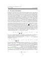
Figure 2: Error estimation for two free parameters. As it can be seen, the parabolic
approximation is valid only in domain U, where the parabolas Γ1 , Γ2 are good approximations of the sections of the χ2 (P1 , P2 ) with planes parallel to P1 and P2
respectively. The true error for the given confidence level is given the bounding
rectangle ABCD of
‘elevation’ line. The confi£ V which
¤ is the
£ corresponding
¤
dence intervals are P1A , P1B and P2D , P2A .
should be calculated numerically, which may have quite unacceptable errors in
some regions of the parameter space (see subsection 2.6.4).
Another approach is the bootstrap method [9, 10, 11, 12, 13] (see section 15.6.
of [18]) using synthetic data sets generated by Monte Carlo methods. We may
generate synthetic data sets from the measured data sets:
• randomly erasing some data points, or
• randomly replacing some data points (this can be used only, if we have several measurements for the same independent variable) with another measurement value, or
• replacing the measured values yiexp with yi∗exp generated as it would have
been drawn randomly from a ‘bootstrap sample’ whose mean is yiexp and
its elements are distributed according to the distribution assumed for the
12
U SER M ANUAL OF F IT S UITE 1.0.4
July 18, 2009
S AJTI Szilárd
experimental data. Therefore we may have to know besides yiexp all the
other parameters on which the distribution depends. E.g. in case of normally
distributed data we have to now the deviation (i.e. the errors of the data), but
yiexp is enough in case of Poisson distributed data, as that already determines
unequivocally the distribution.
The synthetic data sets, which in principle could also be the results of the experiments performed (with the known errors), are fitted. The results of the fit of a
synthetic data set is stored only if it was convergent and the corresponding fitted statistic differs from the fitted statistic of the experimental data set less than a
user defined small positive number. We filter out this way the synthetic data sets
which give a very different fitted statistic, because they miss already too much
information compared to the real experimental
the data points
¯P ³ data, or because
´¯
¯
exp
synth ¯
were not changed really randomly, e.g. ¯
yi − yi
¯ becomes unacceptably large because of a ‘synthetic systematic error.’ It may also happen, that the
fit has gone wrong unexpectedly, and we do not want to throw out everything just
because a few such bad fits. (If the fitted statistic of a synthetic data is less, than
the value used in the ‘filtering criterion’, that value is updated with it. Therefore,
the bootstrap method may also be used as some sort of fitting method.)
Applying this algorithm, we survey the ‘basin’ in the parameter space which
contains the parameter vectors providing fits with the same quality for some possible outputs of our experiment(s) according to the experimental results and our
knowledge about the precision of the measurement. Therefore using the set of
fitted parameter vectors of synthetic data sets, we may get a probability density
(histogram) f (p) corresponding to possible experimental errors. Knowing f (p)
we can calculate the expectation value and the standard deviation of fitted parameters. This standard deviation can be used as an error estimate. The bootstrap
method needs a lot of (' 2000) synthetic data sets,1 therefore it may be very
expensive in computation time. It is advisable to calculate errors only when we
have a quite good fit. For usability conditions and further details of the bootstrap
method see the cited works.
It is inappropriate to give just the errors for a given confidence level, as we may
never know, when somebody will need our data with higher our lower confidence
levels. In that case it is very useful to have the errors for quantile=1, which is the
sample standard deviation, as thereafter the errors knowing the degree of freedom
can be calculated for arbitrary confidence level easily.
The covariance matrix has other uses, than the error estimation. We can ‘discover’ interdependencies between the parameters looking for off-diagonal elements with large (>0) absolute values compared to the corresponding diagonal
1
The number 2000 is not graved in stone, in literature we may find lower values. This depends
on the problem, on the paper.
13
U SER M ANUAL OF F IT S UITE 1.0.4
July 18, 2009
S AJTI Szilárd
elements. In case of such interdependency the transformation matrix technique
may be useful.
2.6 Fitting
Without going into the details here, we try to summarize the approaches used to
fit experimental data sets using optimization methods, enhancing the facts, which
may be important even for the users, who sorrily do not know (and maybe would
not like to know) the mathematical background scrupulously. For further details
we refer to the rich literature about this topic. E.g.: Numerical Recipes in C [15]
available at http://www.nrbook.com/b Chapter 10, or as a good starting point see the
optimization page on Wikipedia and the references available there.
We use optimization method, as fitting parameters we want to find the parameters for which the fitted statistic assumes its minimum. As the fitted statistics
are positive definite such minimum should exist, but there maybe several one, and
a lot of local minima. Therefore finding the global minimum(ma) of a general
function depending on a lot of parameters (variables) is not easy. There is no perfect solution, user interaction, intuition is needed. In case of fitting we usually
have some preliminary knowledge about most of the fitted parameter values, and
we want just to have more accurate values, and to determine only a few totally
unknown parameters, and even in that case we may have some conjecture about
the range in which we should look after them. (Preliminary simulations may be
very helpful at this stage.) We start the fitting from a point of the parameter space,
which according to expectation is not too far from the solution we are looking
for. If we have luck the method will find it, or will get nearer to the solution.
The method may stuck in a local minimum, or in more unlucky cases the method
may become divergent, or it may need further iteration, to get closer to the minimum. To understand these features, we have to tell more about these methods.
It is common in all of them, that they are some sort of iteration algorithms. And
that in each iteration step, the value (and/or derivatives) of the objective function,
whose minimum is to be found, are calculated in discrete points of the parameter
space determined by the method and it is tried to determine, whether is there a
minimum, or where we have to take up the new points, in which the objective
function should be examined next. If we look at the path of the iteration steps
getting nearer and nearer to the current minimum, we will get a curve similar (except of some jitter) to a meandering river flowing always to lower levels. It may
be imagined, that this path may be quite complex in higher dimensions. Reaching
the minimum can take a lot of time and we may stuck into local minima much
easier. As we can examine the function only at finite number of points, if the
resolution of the method (specified by proper options) is not high enough we may
even step over some minima, if it is too high it may take much longer time to
14
U SER M ANUAL OF F IT S UITE 1.0.4
July 18, 2009
S AJTI Szilárd
get there. The methods were devised to make the best possible compromise, but
they are not perfect. It is the task of the user to influence the fitting by setting the
proper options of the method appropriately.
2.6.1 Constraints (Simple bounds)
As we mentioned in the beginning knowing approximately the domain in which
the parameters may be found, can be very helpful. We can add to our optimization
problem constraints of the form gj (P) 6 0. To solve such optimization problems
with constraints, several methods were devised. Here we do not dive into the
nonlinear programming, which tackles the most general problems. We will show
only three simple methods, two of which are used currently in our program. We
have currently only simple bounds, in which case gj (P) = Pij − cj 6 0, or
gj (P) = −Pij −cj 6 0, where cj -s are constants, simplifying the problem further.
The first two methods, the penalty and barrier methods have common features,
as in both cases the objective function is modified. In both cases we replace the
problem with a series of unconstrained optimization problems which should converge to the original problem. We will have a sequence of objective functions of
form
Hk (P) = f (P) + qk Z(P), qk > qk−1 > 0, qk → ∞
(21)
where f (P) is the original objective function, Z(P) is the penalty function and qk
is the monotonically increasing divergent sequence of penalty coefficients. If M
is the feasible region in the parameter space given by the constraints the penalty
function should be of the form
½
0 P∈M
(22)
Z(P) =
>0 P∈
/M
Two often used examples for such penalty functions with m constraints:
Z(P) = (max{0, g1 (P), . . . , gm (P)} + 1)r − 1
and
Z(P) =
m
X
(max{0, gi (P)} + 1)r − m
(r = 1, 2, 3, . . . )
(r = 1, 2, 3, . . . ).
(23)
(24)
i=1
Solving the modified optimization problems consecutively, each time starting from
the solution of the previous modified problem, we may get close to the real solution of the original constrained problem.
With barrier method we have a sequence of objective functions of form
Hk (P) = f (P) + wk B(P),
15
0 < wk < wk−1 ,
wk → 0
(25)
U SER M ANUAL OF F IT S UITE 1.0.4
July 18, 2009
S AJTI Szilárd
where f (P) is the original objective function, wk is the sequence of monotonically
decreasing barrier coefficients converging to 0 and B(P) is the barrier function
growing to ∞ on the boundary of M . Because of this property of the barrier
function it is useful in case of gj (P) < 0 constraints, but numerically (as we have
always a finite precision using computers) there is not much difference between
gj (P) < 0 and gj (P) 6 0. Two often used examples for such barrier functions
with m constraints:
m
X
− ln (gi (P))
B(P) = −
(26)
i=1
and
B(P) =
m
X
i=1
1
(gi (P))r
(r = 1, 2, 3, . . . ).
(27)
In contrast with the penalty method the fitting program using the barrier method
may not get out of the domain defined by constraints. (This is not quite the case
working numerically.) This feature may be especially useful, if the calculated
spectrum as a mathematical function of parameters has a finite domain, out of
which we may get into unpredictable problems.
The third method handling the constraints is quite different. We use our fitting method for problems without constraints, but we check, in each iteration step
whether we are out from the feasible region. If we are out, we continue with the
nearest parameter vector on the boundary on the feasible set and if the method
uses also gradient we continue with the component of the gradient projected on
the boundary. This method is almost the projected gradient method (see e.g. [14]),
but may also be used in case of optimization methods without derivatives. This
projection method is much faster, than the barrier or penalty method, but it may
have its own problems. If some constraint cuts through a bend belonging to the
‘path’ obtained connecting the steps of the optimization method, we may get an
artificial local minimum on the boundary, where the method may stuck (see Fig.
4). In case of a very complex, meandering path, lot of constraints, parameters to
fit, the number of such artificial local minima is multiplied. Therefore we should
be cautious using constraints. Although the usage of the penalty and barrier methods is a bit safer in this regard, but this problem may also arise there.
To use the penalty or barrier function method in case of ‘vector statistics’
defined by (16-20) should be modified, during fitting. E.g. in case of penalty
function, we should replace in these equations κi by
r
qk
,
κi = κ2i + Z(P), i = 1, . . . , n.
(28)
n
16
U SER M ANUAL OF F IT S UITE 1.0.4
July 18, 2009
S AJTI Szilárd
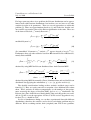
Figure 4: Demonstration of artificial local minimum arising because of constraint
on a contourplot, where the contours denote decreasing levels approaching the
real minimum C. Without the bound represented by line Γ for parameter P1 , the
fitting started from A would be finished in C, but because of bounds it will be
finished in B.
2.6.2 Distributed parameters (using maximum entropy principle)
To fitting problems with distributed parameters, we minimize the fitted statistic χ2∗
and maximize the entropy S of the distribution, therefore we minimize χ2∗ − S. As
we prefer positive definite objective function f obj , remember on vector statistics
defined in (16-20), instead of this we minimize
f
obj
=
χ2∗
+ Smax − S =
χ2∗
+ ln N +
N
X
hi ln hi ,
(29)
i=1
hi >0
as S is maximal if hi = N1 . If we have distributed parameters, we sum the entropies of the m independent distributions


Nj
m
X
X

(30)
hj,i ln hj,i  .
f obj = χ2∗ +
ln Nj +
j
i=1
hj,i >0
The ‘vector statistics’ defined by (16-20) should be modified similarly to (28), i.e.
we should replace in these equations κi by
r
1
κ,i = κ2i + (Smax − S), i = 1, . . . , n.
(31)
n
17
U SER M ANUAL OF F IT S UITE 1.0.4
July 18, 2009
S AJTI Szilárd
The penalty (or barrier) function can be added the same way too.
P In order to fulfill automatically the constraintsRRi h> 0, hj1 ,...,jn > 0 and
hj1 ,...,jn = 1, we fit instead of these parameters πi , πj1 ,...,jn and calculate from
these R and h using the formulae:
¡ R ¢2
πi
¡ h
¢2
πj1 ,...,jn
= P¡
¢2 ,
πjh1 ,...,jn
Ri =
hj1 ,...,jn
(32)
(33)
which give the definition of ‘π’ parameters as well. This is working correctly, but
sometimes, we may experience a bit different behaviour fitting these distribution
parameters compared to the normal parameters.
2.6.3 Rescaling parameters
The expected order of magnitude may also be a helpful information during optimization (fitting), as there are methods (most of them) which do not work properly
(they may become even divergent) for parameters of different order of magnitude
(see fit using rescaling demo). In these cases we can rescale the parameters P
by dividing each Pi by the corresponding order of magnitude mi and optimizing the modified objective function f m (Pm ) = f (P), according to the rescaled
parameters Pim = Pi /mi .
The parameter bounds give the order of magnitude, only if the signs of the
upper and lower bounds are identical, that is the main reason, why the magnitude
should be provided by the user separately.
2.6.4 Numerical derivatives
Usage of methods using or not using derivatives is another question we should address a bit. Mathematicians usually assume, that we have objective functions,
whose derivatives are known, therefore most of the optimization method uses
them as well. The problem is, that in practice we usually do not have the derivatives in case of complex problems, as we do not have an analytical function, but
we have algorithms, which may use a lot of numerical (iterative) algorithms already (e.g. determining eigenvalues in quantum mechanical problems, as Mössbauer line positions and line strengths calculated from Hamiltonian), and we have
a lot of parameters. Therefore calculating the derivatives requires tremendous
additional work for which we usually do not have time and it may not be worth either. Still we should provide the derivatives for the methods requiring it, therefore
we should do it numerically. The problem is, that because of the finite computer
representation of the numbers and because it needs dividing of a number with a
18
U SER M ANUAL OF F IT S UITE 1.0.4
July 18, 2009
S AJTI Szilárd
small number, numerical differentiation is dangerous, therefore it is avoided in
numerical computations whenever possible.
The method implemented by us uses the same trick, as the Romberg‘s method
for integration (see [17], http://www.nrbook.com/b section 4.3. or wikipedia), to get
∞
P
di
high precision derivatives. We know, that f (x0 + h) = f (x0 ) +
hi dx
i f (x0 ),
i=1
therefore using the notation
∞
D0h f (x0 )
X
f (x0 + h) − f (x0 − h)
d
d2i+1
=
=
f (x0 ) +
h2i 2i+1 f (x0 )
2h
dx
dx
i=1
d
=
f (x0 ) + O(h2 ),
dx
(34)
where we use the big O notation, O(h2 ) should be read as order of h2 . We can
eliminate the higher order terms, as in Romberg integration. E.g.:
f (x0 + h) − f (x0 − h) f (x0 + 2h) − f (x0 − 2h)
−
2h
4h
=
3
4D0h f (x0 ) − D02h f (x0 )
d
=
=
f (x0 ) + O(h4 ).
4−1
dx
Generally we may use
D1h f (x0 )
4
Dk>0
h f (x0 ) =
k−1
4k Dk−1
d
h f (x0 ) − D2h f (x0 )
=
f (x0 ) + O(h2k ).
k
4 −1
dx
(35)
(36)
In order
with accuracy O(h2k ) we need 2k function evaluation,
simu¡ to calculate
¢
k
k−1
k−1
k
lation f (x0 − 2 h), f (x0 − 2 h), . . . , f (x0 + 2 h), f (x0 + 2 h) for derivatives and one to get f (x0 ), which may be slow the fitting very much. If we fit several parameters and therefore we have to calculate several partial derivatives, the
program will slow even further. And even then in general case we cannot guarantee, that the function has not a very great high order derivative, which deteriorates
everything. We may check the convergence comparing different order of approximations. E.g. we may accept and stop calculating approximations of higher order
if
¯¢
¯ ¯
¯
¯ k
¡¯
¯Dh f (x0 ) − Dk−1 f (x0 )¯ < C ¯Dkh f (x0 )¯ + ¯Dk−1 f (x0 )¯ ,
(37)
h
h
where 0 < C < 1 is a small number giving the user required precision. It is
useful to have a maximum for the order of approximations, as numerically we
cannot take h arbitrarily small (at least not without extra work and computation
time which is the cost of using a library using numbers with arbitrary precision).
The most plausible choice for h would be |x0 |ε (for x0 6= 0) which is defined as
1 + ε being the smallest number which may be differentiated from 1 for a given
machine precision, but the user may have other choice.
19
U SER M ANUAL OF F IT S UITE 1.0.4
July 18, 2009
S AJTI Szilárd
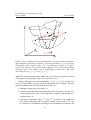
Figure 6: Two subspectra s1, s2, the total calculated Mössbauer spectrum and the
corresponding data set.
2.7 Subspectrum
Sometimes it is useful to see what is the contribution of the parts of the studied
system to the whole spectrum. Therefore Mössbauer spectroscopists devised the
concept of subspectrum. In Mössbauer spectroscopy the contributions of different
sites (atomic environments of the Mössbauer isotope) of the sample are added
up weighted by their concentration calculating the ‘absorption coefficient’ used to
determine the spectrum of the system. Therefore plotting spectrum and subspectra
Fig. 6, i.e. the spectra calculated taking into account only one (or a few, but not
all) of the sites, we may see which site is corresponding to a specific peak, etc.
The subspectrum in FitSuite is a spectrum, where some of the physical objects of the studied system are not taken into account. This concept may also be
helpful (in better understanding of the studied physical system) in cases different
from Mössbauer spectroscopy, even if the whole spectrum cannot be obtained as
weighted sum of single contributions, subspectra. (see subspectrum demo)
3 Working with FitSuite
In the following we try to show the features, the usage of the program in an order, as a new user should go step by step through the different interfaces of the
20
U SER M ANUAL OF F IT S UITE 1.0.4
July 18, 2009
S AJTI Szilárd
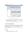
Figure 8: Model Editor: the part used to build up the structure represented by a
tree.
program.
3.1 Starting a new project
Starting the program, the user can start a new project (File | New Project) or load
(File | Open) a previously saved one. The extension of the project files is ‘.sfp’
(simultaneous fit project). We can save our project anytime clicking File | Save. . . .
If we have a new (empty) project, we have to add models (theories in EFFI
terminology). This can be done in two ways. The user can load it from a ‘*.mod’
file (if there is such available, e.g.: such files may be created by exporting), or
you can click Add | New Model and then can choose from a list. The model
appears with an initial name ‘Modeli’ (i = 0, 1, . . .) in the window Problems on
the left of the main window (see Fig. 8). You can change the name clicking on
the text ‘Modeli’ and typing the new name in this window. Please do not use
whitespaces (space, tabulator etc.) in names in FitSuite, as it may have very queer
consequences. Currently only ASCII characters may be used in names. Using
other type of characters may have undesired side effects. (see model definition
demo)
21
U SER M ANUAL OF F IT S UITE 1.0.4
July 18, 2009
S AJTI Szilárd
Figure 10: Model Editor: the part used to choose the correlation functions
3.2 Building up the model structure
On the right side of the main window (Fig. 8) should be seen a Model Editor
now. In this we can build up the hierarchical structure of the model.
On the top is always one object the experimental scheme. We can add other
objects to this (and to every object) with right clicking on it (them) and choosing
Add or Insert from the arising pop-up menu. If there are more than one possibilities, you may choose by moving the mouse on Add . . . . In the current built in
types of models only the layers may be grouped. Selecting them with SHIFT +
cursors or SHIFT + mouse and right clicking on selection you can choose Group
from the pop-up menu. In case of the objects representing the groups the column
labelled with Nrep contains the repetition number telling us, how many times the
elements of the group are repeated in the real physical system. This could be
changed with right clicking on it in previous versions. Now you can change it
setting the corresponding integer parameter (see later).
In case of off-specular (synchrotron Mössbauer reflection) problems we have
to give the correlation functions between the domains belonging to different layers. The domains available at the level of scheme can be linked to the layers.
The correlation functions can be chosen with the help of graphical user interface,
which appears after clicking on tab with label "Correlation function" on the bottom of the model editor (see Fig. 10).
22
U SER M ANUAL OF F IT S UITE 1.0.4
July 18, 2009
S AJTI Szilárd
3.3 Adding data
We can import from files the experimental data selecting the menu item Add |
Data, after this we can choose the format of the file e.g.: ‘one column’, ‘two
columns’, ‘three columns’, ‘compact’ (I name so, as I could not find better name,
the format:
0
5
10
68348
68198
67436
68699
68508
67776
68315
67983
68123
68375
68114
68143
68253
68041
68480.
E.g. see the files 4k0t.dat, 4k3t.dat, 4k5t.dat in directory adatok), etc. We can
give the line with which the reading begins (First line to read in) (the numbering
starts with 0!), the number of lines we want to read in (if it is 0 then it will read
all) and we may give a string (this of course could be a number) until whose first
occurrence (after the line which was given in First line to read in) we want to
read in the lines. Presently the program does not read parameters, constants from
data file. In compact format we can add the number of data columns, in the above
mentioned example this is 5, as the first column (0, 5, 10, . . . ) gives the number
of data in former lines. (see reading ASCII data file demo)
Scans from Certified Scientific Software’s specTM (X-Ray Diffraction and
Data Acquisition software) files can be obtained in another way from version
1.4.1. on. Open spec file clicking (File | Open spec File), wereafter a window
should appear, where you may (filter) select the scans and extract the chosen data
sets. If the required spec file has already been opened, it is enough to choose the
menu item (View | Show Open spec Files), to have this window. Extraction types
may be defined, changed. For further details see this spec file demo.
The experimental data have some distribution. E.g. data obtained using particle counters usually have Poisson distribution. ‘Ordinary’ experimental data are
expected to have Gaussian distribution. Fitting the experimental data, we have
to know, which distribution should be used as the fitted statistics should be chosen accordingly. The type of the distribution can be chosen here or later. If the
imported data contains errors too we may set its type (root mean square or mean
square) as well. Sometimes the raw data is already preprocessed. E.g. neutron
reflectometrists usually normalize their data, as they measure reflection, which
has a maximal value of 1. The problem with this preprocessing is that in case of
Poisson distribution we throw out this way information (see subsubsection 2.4).
Therefore here you can tackle this problem by providing the normalization factor
if there was such one. This piece of information may be provided later as well.
Right clicking in the window Problems on the name of the new dataset, we can
add the data to the chosen model. At present, the user should know which format
23
U SER M ANUAL OF F IT S UITE 1.0.4
July 18, 2009
S AJTI Szilárd
is required, accepted by a given type of model. If you choose a wrong one it
will warn you only with malfunctioning or with segmentation fault error message.
Data set may be replaced right clicking on the name of data set and clicking on
Replace Data in the arising menu. This is useful if there was a mistake made by
the user choosing, reading the data set, or after cloning (see later).
Some data points may be ex(in)cluded from the fit selecting with SHIFT +
cursor and right clicking. This can be used if you are sure that some values are
badly measured. The exclusion is not working correctly for all the models at the
moment, do not use it in case of Mössbauer and stroboscopy spectra. From version
1.0.3 on you may exclude data points according to their values as well.
The user may also add his(er) notes to the data after clicking on button Notes
at the bottom of the data window.
The above mentioned statistical properties of the data set can be changed clicking on button Statistical Properties at the bottom of the data window. Here you
can choose the distribution of the data set. Set the normalization factor, if there
is such one (preprocessed data). Besides the user may choose the statistic, whose
minimum has to be found by fitting the parameters, and the GOF (goodness of fit)
statistic. For further details see 2.4.
3.4 Changing parameters, matrices
From version 1.0.3 the parameters and transformation matrices are generated automatically. With Edit | Regenerate Matrices you may generate them, if there is
some problem, or you want to set the transformation matrices starting from the
initial ones. The parameters and the matrices may be changed with Edit | . . . . For
the program generated parameter (variable) names the following name convention
is used:
• For the parameters of simple physical objects:
ModelName=>ObjectName:>PropertyName::ComponentName.
E.g.: FirstProblem=>SecondIncoherentFraction:>ExternalMagneticField::x.
• In case a linked objects (e.g.: domains in off-specular problem):
Model=>ParentObject*>LinkedObject:>Property::Component.
E.g.: FirstProblem=>ithLayer*>jthDomain:>size.
• In case of correlation function parameters of two linked objects:
Model=>FirstParent*>FirstLinkedObject,SecondParent*>SecondLinkedObject>>
FunctionTypeName:>Property::Component.
E.g.: FirstProblem=>ithLayer*>jthDomain,lthLayer*>mthDomain>>Gauss:>sigma.
In Parameter Editor (Edit | Fitting Parameters) everything is included what
is not integer independently on being constant or not. The parameters with check
24
U SER M ANUAL OF F IT S UITE 1.0.4
July 18, 2009
S AJTI Szilárd
Figure 12: Parameter Editor
√
boxes (change them by double click) filled with ‘x’ (Linux) or ‘ ’ (Windows)
denote the free parameters. The constants do not have check boxes, thus they cannot be freed. There are calibration constants, user defined constants and model
defined constants. Calibration constants have a label ‘ca’ instead of check box.
They may be fitted right clicking on the check box or selecting the appropriate
calibration constants (SHIFT + cursor) + right clicking and selecting ‘Let Not Be
Constant’ from the arising menu. The user may set arbitrary parameters to be
constant, by choosing in this menu ‘Let Be Constant’. If the parameter was not a
calibration constant, the check box will replaced by ‘c’, these are the user defined
constants. There may be constants, which are never fitted, these are denoted by
label ‘cn’, these are the model defined constants. (see free/fix, make constant parameter demo) To increase the transparency of the parameter list the user may hide
parameters, which (s)he thinks have the correct value and will not be fitted. This
can be done similarly to previous operations, just a different menu item should be
chosen. For obvious reasons free parameters may not be hidden and hidden parameters may not freed. The hidden parameters may be seen pressing the proper
button (or menu item) appearing after parameters were hidden. The hidden parameters will appear with a different background color. This color may be changed in
the Editor Settings (Settings | Editor Settings) (see hidding parameters demo).
From version 1.0.3 the parameters may have units. In older project files they
will appear only after the command Edit | Regenerate Matrices was given for the
program. (Sorrily with this the transformation matrices changed by the user will
be lost and should be made again.) The units may be changed several ways. Just
25
U SER M ANUAL OF F IT S UITE 1.0.4
July 18, 2009
S AJTI Szilárd
double clicking on the unit in the parameter editor, the unit may be changed. If
the button with an arrow is pressed down, not only the unit is changed, but the
parameter value is also converted from the previous unit to the new one. Editing
a parameter value with units, the unit may also be changed. In this case pressing
down the button with arrow, the new unit and value is set, there is no conversion.
If the button is not pressed down the unit remains the original one, but the value
will correspond to the selected value and unit converted to the original one. (see
parameter values and units demo) You may change the units of the minimum,
maximum and magnitude (the latter is used to rescaling) values as well. If these
units are identical with the unit of the parameter value, they are represented by
shortcut ~. The user is able to specify a bit the behaviour of unit editor in Settings
| Editor Settings (see editor settings demo).
You can get some information about the parameters by first clicking Help |
What is this? or pressing SHIFT+F1, (on this the cursor icon should change to a
question mark), clicking thereafter on the parameter name in the editor a short help
should appear. Presently, this type of help is not complete, for some problems,
e.g.: stroboscopic mode problems there is nothing available.
The displayed numbers in Parameter Editor and in Transformation Matrix
Editor (Edit | T Matrices) also are rounded to a few digits. If a number is longer
than that, the rounded number is displayed in blue (or other user set color) and
we can see the real (not rounded) value by pulling the mouse over that cell in
the editor and waiting until it appears in a tooltip. The user is able to specify the
number of the displayed digits, choose the precision, what he needs and a lot of
other options in Settings | Editor Settings.
In current version, the matrices can be united, split, and the parameters can be
correlated, decorrelated and user defined parameters may be inserted (see subsection 2.2 and the demos of parameter correlation, decorrelation1, decorrelation2
and matrix split-unite).
The handling of integer parameters and the related integer transformation matrices may be handled quite similarly. The main difference is, that there we have
to use the Integer Parameter Editor (Edit | Integer Parameters) and similarly
the Integer Transformation Matrix Editor (Edit | Integer T Matrices).
3.5 Report generator
On clicking Results | Create Report appears a window with a report of the current
project containing the model structure and the model parameter values. The report
can be saved in an html file. (This feature is still in a very early development
stage.)
26
U SER M ANUAL OF F IT S UITE 1.0.4
July 18, 2009
S AJTI Szilárd
Figure 14: Transformation Matrix Editor
3.6 Cloning
It happens frequently that the user wants to fit the same type of experiment in a
bit different environment, or a bit different sample, etc. It would be inconvenient
to build up almost the same model several times and then to correlate almost all
the parameters. Therefore in FitSuite we can clone the models. This can be done
by just right clicking on the model name in the window Problems and selecting
Clone from the pop-up menu. Thereafter a dialog arises in which we can choose
the number of clones and the parameters and/or matrices which are (not to) to be
correlated. After this we will have copies of the chosen model and of the data
belonging to it. These data may be replaced by right clicking on them in the
window Problems and choosing Replace Data from arising pop-up menu.
3.7 Model groups
The user may group models from version 1.0.3. The model groups are used just
to select a few models from the available ones in the current project, in order
to simulate, fit, plot only them. To create model groups just select them in the
window Problems with SHIFT+cursor, right click with mouse and in the arising
27
U SER M ANUAL OF F IT S UITE 1.0.4
July 18, 2009
S AJTI Szilárd
pop-up menu select Group Model(s). In the dialog showing up thereafter the user
may choose the models to be grouped and the name of the group according to
which we can use them later on see modelgroup demo.
3.8 Simulation, Fit
The simulation can be started by clicking Fit/Simulation | Simulate. The program
checks, whether there was a former simulation, and the parameter values were
changed or not, and calculates only when it is necessary. It may happen that this
program decision was not appropriate. In such cases you may force simulation
by clicking Fit/Simulation | Force Simulation. It is possible to simulate only a
single model (fitting problem), or models of a model group (see subsubsection
3.7) choosing the proper menu items of Fit/Simulation | Simulate Only . . . and
Fit/Simulation | Force Simulation of . . . .
The independent variable of the simulation/fit may be specified by setting
properly in the Problems window on the left side in the column with name grid
type, if there is a possibility. Just click on the proper cell, and change it, if it is
possible.
The iteration (fitting) can be started by clicking Fit/Simulation | Fit. It is possible to fit only a single model (fitting problem), or models of a model group
choosing the proper menu items of Fit/Simulation | Fit Only . . . .
Choosing the menu item Fit/Simulation | Select Method you can select the
fitting method and set their parameters. At present we have the following methods:
• Powell‘s method which is a slightly modified version of the code available
in Numerical Recipes in C available at http://www.nrbook.com/b section 10.5.
The method has parameters, options, which appear if the Details button is
pressed down. These options are the following:
– MaxIter: is the maximum number of iteration steps, if a minimum was
not found in so many steps, the optimization is finished.
– tolerance: is the tolerance ftol with which the minima of the function
f is determined. The result fn of the nth iteration step is accepted if
ftol (|fn−1 | + |fn |) > (fn−1 − fn ).
Powell‘s method uses line minimization methods, as Golden-section search
(see in Numerical Recipes in C available at http://www.nrbook.com/b section
10.1 and/or on on Wikipedia), Brent‘s method (brent), Brent‘s method using
derivatives (dbrent)(see in Numerical Recipes in C section 10.2 and 10.3,
respectively). The user may be choose one of them. They and their parameters appear on the interface if the second (1-dim optimization method)
Details button is pressed down. They have the following parameters:
28
U SER M ANUAL OF F IT S UITE 1.0.4
July 18, 2009
S AJTI Szilárd
– MaxIterLine: is the maximum number of iteration steps in the 1 dimensional optimization method, if a minimum was not found in so
many steps, the current line optimization is finished. (The main method
may continue its own iteration. The fitting is not finished just because
MaxIterLine was reached.)
– tolLine: is the fractional tolerance tLine with which the minimum along
the given direction should be found by brent or dbrent method. Optimization along a direction is finished if 2tLine |x| > |x0 − x| , where x0
is the true local minimum and x is the calculated one.
– GLimit: In the optimization methods Powell, Fletcher – Reeves and
Polak – Ribiere the minimum of the function f (which in case of fitting of experimental data sets is the χ2 ) is searched along directions
specified by them. The first step to find a minimum along a direction is to find three points a, b and c where b is between a and c furthermore f (a) and f (c) are both greater than f (b). The three points
are searched by starting from an initial triplet moving similarly to an
inchworm, i.e. updating (a, b, c) by (a = b, b = c, c = u), where u
is the minima of the parabolic fit on (a, f (a); (b, f (b)); (c, f (c)).
This type of move is accepted only if the obtained u is between c and
ulim = b + GLimit (c − b), otherwise the (a = b, b = c, c = ulim ) move is
made. This is quite oversimplified just to explain the use of GLimit.
For further details see the routine mnbrak in ‘Numerical Recipes in C
(Fortran)’.
• Nelder – Mead method (Numerical Recipes in C based, section 10.4). A
good description, with animation is available on wikipedia. Nelder – Mead
method is sensitive to scaling of the parameters. It has the following parameters and options (appearing on the interface if Details button is pressed
down):
– MaxIter: as in Powell‘s method.
– tolerance: as in Powell‘s method.
– Initial simplex size: is a parameter determining the length of the vectors pointing to the vertices of the simplex from the initial parameter
vector (consisted only the free components).
– Reflection factor: see Numerical Recipes in C
– Stretch factor: see Numerical Recipes in C
– Contraction factor: see Numerical Recipes in C
29
U SER M ANUAL OF F IT S UITE 1.0.4
July 18, 2009
S AJTI Szilárd
• Polak – Ribiere and Fletcher – Reeves methods (Numerical Recipes in C based,
section 10.6 and on wikipedia). They have the same options and parameters
as Powell‘s method.
• Broyden – Fletcher – Goldfarb – Shanno (on wikipedia) variant of the Davidson – Fletcher – Powell method (Numerical Recipes in C based, section 10.7,
may see also on wikipedia). It has the following parameters and options
(appearing on the interface if Details button is pressed down):
– MaxIter: as in Powell‘s method.
– MaxStep: is the scaled maximum step length allowed in line searches
in BFGS. For further details see stpmx variable in the corresponding
Numerical Recipes in C function (Fortran subroutine).
– Alpha: ensures sufficient decrease in function value in line searches
in BFGS. For further details see ALF variable in the corresponding
Numerical Recipes in C function (Fortran subroutine).
– TolxLnsrch: gives convergence criterion on the location of the minimum in line searches in BFGS. For further details see TOLX variable
in the corresponding Numerical Recipes in C function (Fortran subroutine).
• Levenberg – Marquardt method (Numerical Recipes in C based, section 15.5
may see also on wikipedia).
• Levenberg – Marquardt method (LMDER) from the MINPACK [4, 5] package available at http://www.netlib.org/minpack/. This was translated from Fortran into C++ and modified a bit by us, so it may work a bit differently, than
the original one.
• N2F, N2FB, N2G, N2GB (based on NL2SOL [6, 7]) from PORT package
available with documentation at http://www.bell-labs.com/project/PORT (for
some reason, this is often unreachable, try it). These were translated from
Fortran into C++ and modified a bit by us, so it may work a bit differently,
than the original ones. Here are a lot of parameters, which are not always
easy to set and these methods were not tested in FitSuite extensively. On
64 bit Linux it is not working at all.
If the result of the iteration is not what you like, you can get back the state before
the iteration by clicking Fit/Simulation | Revert. Before a fit is started the project
is saved in the file *.sfp~, which is loaded on the command Revert.
From version 1.0.4 the results are not written in files automatically. They may
be exported using the menu items Results | Export .... You may choose the data
30
U SER M ANUAL OF F IT S UITE 1.0.4
July 18, 2009
S AJTI Szilárd
which should be exported, and set the format of the created files using (Settings |
Export Settings)
3.9 Error calculation
Errors of free parameters may be calculated clicking Fit/Simulation | Calculate
Errors. There are currently two approaches used in the program for this purpose.
One is based on covariance matrix, the other is named bootstrap method (be aware
that bootstrap method is very expensive in computation time). Explanation of the
principles of these method can be found in Numerical Recipes in C available at
http://www.nrbook.com/b section 15.6. You may choose one of them (or both) by
proper settings after clicking menu item Fit/Simulation | Select Method, on the
page with title Parameter Errors. Here, you may also change the required confidence level. Still in the same dialog on page with title Bootstrap method you
can set the parameters used by bootstrap method, namely the number of synthetic
data sets and the convergence criterion. According to the literature the number
of synthetic data sets should be (at least) about a few thousands, the current default value is 200, as we used most only for testing and because of the slowness
of this method. The convergence criterion gives the criterion to stop the fitting
of a synthetic data sets, if the difference of fitted statistics belonging to the real
experimental and the current synthetic data sets is smaller than this. Bootstrap
method needs errors of the experimental data, without that will not work appropriately. If the experimental data has Poisson distribution, it is enough just to
set the distribution properly.
3.10 Calculating statistics
to be written
3.11 Plotting
(Originally it was planned to use gnuplot for plotting of the results. That way we
could have more beautiful and appropriate (‘press ready’) graphs. The problem
is that it is a bit circumstantial to get control over the plot windows created by
gnuplot. There is a solution, but only for X11 systems and that would not be
portable. Therefore we use the open source plot library Qwt which is based on Qt.
This can be integrated in FitSuite and developed further without problems. It is
not as beautiful as gnuplot, but it should be enough during fitting or simulations.)
Presently, the (Qwt based) plot windows are created (if they are not available
already), when an iteration is started. The data and the results of simulations before and after each iteration are plotted. The theoretical results are represented by
31
U SER M ANUAL OF F IT S UITE 1.0.4
July 18, 2009
S AJTI Szilárd
their ordinal numbers and with different colours in the plot legend. Clicking on
the corresponding part of the legends the user may hide(show) the corresponding
curves. Right clicking on the plot window, the user may zoom in (out) a selected
(first click on zoom in in the pop-up menu and after that select with mouse) rectangular region of the plot. You may choose logarithmic scale for y axes, but this
is not always perfect, as in Qwt it is done in a bit queer way (this may be changed
in next versions of FitSuite). The colors can be set, changed in pop-up also clicking on Change Line Colors. Here you can change the available colors and add
new ones to the list. Pushing the button Set default you save these settings on
the computer, in order to have the same colors when you start FitSuite next time.
For offspecular problems [8] we have spectrograms, and contours, which can be
changed similarly. But in these cases, the levels should be set also, these may be
chosen to be elements of a geometric or arithmetic sequence, by clicking in the
menu of the corresponding dialog. In case of spectrograms you may create line
section graphs along the edges of a polygon by choosing from the pop-up menu
Polygon section, pressing the right mouse button you add the first vertex, moving
the mouse to a new point and pressing spacebar a new vertex can be added. Pressing enter or the right mouse button you finish the polygon. In the profile window
you may need to choose logarithmic scale. The created line section profile may
not be appropriate if the axes belonging to the two independent variable have very
different scale, or you have a polygon with too much vertices.
When the user would like to have an image file of the data and the fitted curve,
we recommend gnuplot (or Origin, etc.). From version 1.0.4 the results are not
written in files automatically (if it is not set so in Settings | Export Settings). They
may be exported using the menu items Results | Export .... You may choose the
data which should be exported, and set the format of the created files using (Settings | Export Settings)
Clicking on the menu items Plot | Plot you can choose the model (or model
group) whose simulation/fit result(s) you would like to plot. Plot | Plot All replots
all the simulation(fit) results if you closed the plot windows before, but this works
only if there was a fresh simulation(fit). Plot | Close All closes all the currently
open plot windows.
3.12 Sounds
Currently after the fit was finished a wav sound file is played. If you do not like
this, just select another file or switch it off using Sound Settings (Settings | Sound
Settings). On Linux systems no sound is played.
32
U SER M ANUAL OF F IT S UITE 1.0.4
July 18, 2009
S AJTI Szilárd
3.13 Examples
Presently there are only a few example project files. They can be found in the
directory examples, where we can find several subdirectories. In each one we can
find project files saved at different phase of the project definition process. The
files ending with:
• Simulation.sfp (usually) contain simulations no data,
• Fit.sfp contain fits with data sets,
• Simultan.sfp contain several data sets fitted simultaneously.
In the directory:
• XrayReflectionFePd we can find projects for non-resonant X-ray reflectometry experiments.
• ResonantXraySelfDiffusionFePd and XrayRes_NoResRelectionFeCr we can
find projects for resonant and non-resonant X-ray reflectometry experiments.
• MossbauerSpectraFemtz we can find projects for a Mössbauer experiment.
The project containing simultaneous fitting problems contains three spectra
for which the internal magnetic field Hint and the effective thicknesses of
sites s2 and s3 and a few other parameters were chosen to not to be correlated during cloning.
• SMRStroboscopicMode we can find a project for Stroboscopic Mössbauer
simulations.
• SynchrotronTransmission we can find projects for synchrotron transmission
experiments.
• SynchrotronTimeDifferential we can find projects for a time differential reflection experiment.
• NeutronReflection there are two specular simulation projects CrFeSimulation.sfp and FePdSelfDiffusionSimulation.sfp and two off-specular simulations CrFeOffspecularSimulation.sfp, CrFeOffspecularSimulationModified.sfp. In off-specular case the ‘3dimensional’ results are plotted in a colored map. Usually, the color ranges are not appropriately chosen, but you
change as it is written in the section 3.11. Under Windows (and sometimes
under some Linuces) for some unknown reason there may be a segmentation
fault, if you calculate in too much points. Therefore loading the off-specular
problems set n_omega, n_theta_sca, etc. to smaller values, e.g.: 200 and
200 (or smaller).
33
U SER M ANUAL OF F IT S UITE 1.0.4
July 18, 2009
S AJTI Szilárd
Figure 16: Fitted X-ray reflectometry spectra
• OffspecularResonantXRay is a project simulating off-specular problem for
synchrotron radiation. It is a recently added problem. It takes a long time
even to simulate, fit has not been made, tested.
• miscellaneous some simple functions added, just to test the fitting routines.
4 Sources, documentation
The sources containing the Fortran subroutines, Cfunctions used for simulations
with the libraries created from them can be found in directory Repositories. Their
documentation and the files used as help in the Parameter Editor are also there.
These are still not complete.
The experimental data files are collected in adatok and the project files in
examples.
5 To do
• complete program documentation, User manual
34
U SER M ANUAL OF F IT S UITE 1.0.4
July 18, 2009
S AJTI Szilárd
Figure 18: Off-specular synchrotron Mössbauer reflection simulation.
• write a separate GUI for creation of new (or modification of) model types.
• let be possible to copy models and their parts (the same way as we copy
directories and files) on GUI.
• automatic names (GUI).
• extend plot features (GUI).
– selection of parameters (GUI).
• extend report generator, log file.
• when the independent variable is generated from a parameter, the plot of the
data set should be replotted also.
– test methods, adjust default parameters values, write some usage notes.
• More validators needed to do not allow illegal names (parameter name, object, model, matrix name).
• Have a directory for log file outputs and temporary work files.
35
U SER M ANUAL OF F IT S UITE 1.0.4
July 18, 2009
S AJTI Szilárd
6 ‘Installation’
The current version was tested only under openSuse Linux 11.1 (32 and 64 bit)
and under Windows XP. The program is mainly written and tested under Linux,
therefore the Windows version sorrily is still much more error-prone. In principle
the program can also be compiled for other Linux (Unix) distributions, earlier
(Linux, Windows) versions and Mac
6.1 Linux
Download the setup file fitsuite-1.0.4-LinuxDistribution-architecture.sh from
this ftp site. This is a Self Extracting Tar GZip compressed packages (needs
/bin/sh, tar and gunzip for extracting) and you may need to set the file permission in order to be allowed to execute. This shell script may have the following arguments --prefix=full path to directory were FitSuite should be installed,
--help. After starting the script from a terminal will ask, whether you accept the
license or not, and that ‘Do you want to include the subdirectory fitsuite.1.0.4LinuxDistribution-architecture?’. For the last question answer boldly ‘n’(o), as
the program will be in prefix/FitSuite/1.0.4/. (If the ‘keyboard repeat rate’ is too
fast, it may happen, that the program does not react properly and you cannot
install it, in that case change your personal keyboard configuration . . . ) Start the
program fitsuite.1.0.4 available in this directory. I tried to include all the ‘non standard’ libraries needed by FitSuite, these are installed in prefix/FitSuite/1.0.4/lib,
hopefully there will no problem with this. If the program does not find some of
the libraries available here set using the command ’export LD_LIBRARY_PATH
= prefix/FitSuite/1.0.4/lib:$LD_LIBRARY_PATH’ (use full path!). If other libraries are missed by the program, please check whether they are installed on
your system, etc.
The binary created for X86_64 of course will not run under 32 bit systems, do
not try to run binaries created for later Suse Linux versions in earlier distributions,
as probably the required system, gcc libraries may be too old.
6.2 Windows
Download the setup file fitsuite-1.0.4-Win32.exe from this ftp site, and start it.
7 License
FitSuite is a scientific software provided free as it is under the terms of GNU GPL
license, except for one additional condition: should you use FitSuite to any ex36
U SER M ANUAL OF F IT S UITE 1.0.4
July 18, 2009
S AJTI Szilárd
tent for your publication, you should cite the article on FitSuite currently available
at http://arxiv.org/abs/0907.2805v1, by mentioning also the name of the program
and the version number. (e.g.: FitSuite 1.0.4) The above link will be updated
when the regular journal article will be out. Please use to Forum to disseminate
the bibliographic data of your published papers that make use of FitSuite.
Fitsuite uses the open source version of Qt4 (Qt4 licensing).
Source code of the main program is available on personal request to the author:
([email protected]), since it is essential for us and our funding agencies to
keep track of the distribution. Source code of the routines of the theories are
already included in the binaries.
The program uses 3rdparty libraries Qwt5, LAPACK, TSFIT, these could be
installed by the user. They are included in the directory 3rdParty only in order
to make the ‘installation’ of FitSuite 1.0.4 easier. Qwt has its own license (a
bit modified version of GNU LGPL) given in the file 3rdParty/qwt/COPYING,
for further details see that. TSFIT may be distributed under GNU GPL see 3rdParty/TSFIT/COPYING. For LAPACK see 3rdParty/lapack-3.1.0/COPYING (it
is not GPL but something like that).
37
U SER M ANUAL OF F IT S UITE 1.0.4
July 18, 2009
S AJTI Szilárd
References
[1] H. Spiering, L. Deák, L. Bottyán: ‘EFFINO’ Hyp. Int. (2000) 125 197-204.
doi: 10.1023/A:1012637721433
[2] K. Kulcsár, D.L. Nagy, L. Pócs, in: Proc. Conf. on Mössbauer Spectrometry,
Dresden (1971).
[3] T. Hauschild, M. Jentschel: ‘Comparison of maximum likelihood estimation
and chi-square statistics applied to counting experiments’ Nucl. Instr. and
Meth. A (2001) 457 384-401. doi: 10.1016/S0168-9002(00)00756-7
[4] J. More, B. Garbow, K. Hillstrom: ‘User Guide for MINPACK-1’ Technical
Report ANL-80-74, Argonne National Laboratory, 1980.
[5] J. More, D. Sorenson, B. Garbow, K. Hillstrom: ‘The MINPACK Project’
in ‘Sources and Development of Mathematical Software’, editor W. Cowell
(1984) 88-111.
[6] J.E. Dennis Jr., D.M. Gay and R.E.Welsch: ‘An Adaptive Nonlinear LeastSquares Algorithm’ ACM Trans. Math. Software (1981) 7, 348-368.
[7] J.E. Dennis Jr., D.M. Gay and R.E.Welsch: ‘-Algorithm 573. NL2SOL -An
Adaptive Nonlinear Least-Squares Algorithm’ ACM Trans. Math. Software
(1981) 7, 369-383.
[8] L. Deák, L. Bottyán, D.L. Nagy, H. Spiering, Yu.N. Khaidukov, Y. Yoda
‘Perturbative theory of grazing-incidence diffuse nuclear resonant scattering of synchrotron radiation’ Phys. Rev. B (2007) 76 224420. doi:
10.1103/PhysRevB.76.224420
[9] B. Effron: ‘Bootstrap Methods: Another Look at the Jackknife’ The Annals
of Statistics (1979) 7:1 1-26.
[10] B. Effron: ‘The jackknife, the bootstrap, and other resampling plans’ Society
of Industrial and Applied Mathematics (1982) CBMS-NSF Monographs 38.
[11] B. Effron, R.J. Tibishrani: ‘Bootstrap Metods for Standard Errors, Confidence Intervals, and Other Measures of Statistical Accuracy’ Stat. Sci.
(1986) 1 54-77.
[12] B. Effron, R.J. Tibishrani: ‘An introduction to the bootstrap’ Chapman &
Hall/CRC (1993).
38
U SER M ANUAL OF F IT S UITE 1.0.4
July 18, 2009
S AJTI Szilárd
[13] B. Winkler: ‘Bootstrapping Goodness of Fit Statistics in Loglinear Poisson Models’ Collaborative Research Center (1996) 386, Discussion Paper
53 http://epub.ub.uni-muenchen.de/1449/
[14] C.-J. Lin: ‘Projected Gradient Methods for Non-negative Matrix
Factorization’ Neural Computation (2007) 19:10, 2756-2779. doi:
10.1162/neco.2007.19.10.2756
[15] W.H. Press, S.A. Teukolsky, W.T. Vetterling, B.P. Flannery: ‘Numerical
Recipes in C’ 2. ed. Cambridge University Press (1992) http://www.nrbook.
com/b
[16] W.H. Press, S.A. Teukolsky, W.T. Vetterling, B.P. Flannery: ‘Numerical
Recipes in C’ 2. ed. Cambridge University Press (1992), 683. http://www.
nrbook.com/b
[17] W.H. Press, S.A. Teukolsky, W.T. Vetterling, B.P. Flannery: ‘Numerical
Recipes in C’ 2. ed. Cambridge University Press (1992), 140. http://www.
nrbook.com/b
[18] W.H. Press, S.A. Teukolsky, W.T. Vetterling, B.P. Flannery: ‘Numerical
Recipes in C’ 2. ed. Cambridge University Press (1992), 689-699. http:
//www.nrbook.com/b
[19] B. Window: ‘Mössbauer spectra of Invar alloys’ J. Phys. E: Sci. Instrum. 4
401-402.
[20] J. Hesse, A. Rübartsch: ‘Model independent evaluation of overlapped Mössbauer spectra’ J. Phys. E: Sci. Instrum. (1974) 7 526-532.
[21] G. Le Caër, J.M. Dubois: Evaluation of hyperfine parameter distributions
from overlapped Mössbauer spectra of amorphous alloys J. Phys. E: Sci.
Instrum. (1979) 12 1083-1090.
[22] I. Vincze: Fourier evaluation of broad Mössbauer spectra Nucl. Instr. and
Meth. (1982) 199 247-262.
[23] R.A. Brand, G. Le Caër: ‘Improving the validity of Mössbauer hyperfine parameter distributions: The maximum entropy formalism and its applications’
Nucl. Instr. and Meth. B (1988) 34 272-284.
[24] E.T. Jaynes: ‘Information Theory and Statistical Mechanics’ Phys. Rev.
(1957) 106 620-630.
39
U SER M ANUAL OF F IT S UITE 1.0.4
July 18, 2009
S AJTI Szilárd
[25] E.T. Jaynes: ‘Information Theory and Statistical Mechanics. II’ Phys. Rev.
(1957) 108 170-190.
[26] R. Lieu: ‘Maximum entropy data analysis: another derivation of S − χ2 ’
J. Phys. A: Math. Gen. (1988) 21 L63-L65
[27] R. Lieu, R.B. Hicks, C.J. Bland: ‘Maximum entropy in data analysis with
error-carrying constraints’ J. Phys. A: Math. Gen. (1987) 20 2379-2388
40
U SER M ANUAL OF F IT S UITE 1.0.4
July 18, 2009
S AJTI Szilárd
Glossary
big O notation is used to give the order of magnitude, e.g. O(h2 ) should be read
as order of h2 .
check box is a graphical user interface element (widget) that permits the user to
make multiple selections from a number of options. Normally, check boxes
are shown on the screen as a square box that can contain white space (for
false) or a tick mark or X (for true). (see wikipedia)
correlation is an operation transformation matrix used to eliminate the redundancies arising because of common model parameters, see eq. (1), its inverse is
the decorrelation. (see subsection 2.2)
decorrelation is the inverse of correlation, which is not unequivocal, therefore
further user interaction may be needed. (see subsection 2.2)
degree of freedom (DOF) is the number of data points minus the number of fitted parameters.
distribution midrange is the middle of the distribution range.
distribution range is the width of the histogram, outside of which the approximated distribution is assumed to be negligible.
EFFI (Environment For FItting) is the name of the program written by Hartmut
Spiering.
experimental scheme contains the information necessary for description of the
system consisted of the experimental apparatus(es), about the experimental
method performed with them and of the system under study e.g: a measured
sample. (see subsection 2.1)
extraction type (spec file) is a structure, which may be defined by the user, used
to collect the information needed to extract a scan from a spec file into a
FitSuite data set.
feasible region in case of optimization problems with constraints is the region
in the parameter space determinded by the constraints where the optimum
should be found.
feasible set see feasible region
41
U SER M ANUAL OF F IT S UITE 1.0.4
July 18, 2009
S AJTI Szilárd
fitted statistic In case of simultaneous fitting, we can have experimental data
with different distributions, therefore the statistics used to fit for each fitting problem may be different. We fit a resulting statistic, their (weighted)
sum. This is not a problem, as if we start from the MLE, from which all of
them are derived, we would obtain also such a resulting statistic. In the case
of the resulting statistic, the names like classical χ2 , Pearson‘s χ2 , etc. will
not have any meaning, therefore in the program it is referred to just as the
‘Fitted Statistic’.
goodness-of-fit statistic is a statistic measuring the goodness of a fit. (see subsection 2.4)
GUI Graphical User Interface
integer parameter Some parameters are integer numbers, these are not fitted,
and are handled separately from real number based parameters, in order to
avoid rounding errors.
model is an object to which belong algorithms for calculation of characteristic
spectra. (see subsection 2.1)
model parameters are all the parameters, which are needed by the models in order to calculate the spectra, without using transformation matrix technicque.
Usually there are a lot of common parameters, wherefore transformation
matrix technicque is used. (see subsection 2.2)
object The word object is used in several sense in this text, including its everyday
meaning too. It may mean:
• in most of the cases means a physical object or concept (see the corresponding item in the glossary, and subsection 2.1)),
• a program language concept used in Object Oriented Programming.
objective function is the function whose location of minimum and/or maximum
is to be found by the optimization method.
optimization method is an algorithm used to find the location(s), where a given
function assumes its minimum or maximum.
parameter distribution see subsection 2.3
parameter insertion inserts a new simulation/fit parameter, inserting a new column in the transformation matrix (see subsection 2.2)
42
U SER M ANUAL OF F IT S UITE 1.0.4
July 18, 2009
S AJTI Szilárd
parameter vector is a vector (array) consisted of the simulation/fit or model parameters as components.
penalty function method is a method used for optimization problems with constraints, modifying the objective function by adding penalty functions outsied of the feasible region. (see subsection 2.6.1)
pop-up menu is a menu in a graphical user interface (GUI) that appears upon
user interaction, such as a right mouse click. (see wikipedia)
property Properties in FitSuite represent the physical quantities (thickness, roughness, hyperfine field, susceptibility, EFG, effective thickness, etc.) and some
numbers characterizing the experimental scheme e.g. number of channels,
symmetries of the sites, etc. (see subsection 2.1)
reduced χ2 is the χ2 divided by degree of freedom (see eq. (14))
repetition group (of physical objects) is a group of physical objects, e.g. layers
which (more accurately the same sort of objects) are repeated in the same
order several times.
repetition group number shows how many times the elements of the repetition
group are repeated in the real physical system
root object is at the root of the object tree structure. It is analogous to the root
(main in some operating systems) directory in the filesystems used in computing.
simulation/fit parameters are all the parameters, which using transformation
matrix technicque are needed to calculate the spectra. Optimally the number
of simulation/fit parameters is less than the number of model parameters, as
already some redundancy is eliminated, by proper choice of the transformation matrix. (see subsection 2.2)
spec file is a file format of Certified Scientific Software’s specTM (X-Ray Diffraction and Data Acquisition software) used for experimental data in ESRF and
many other places.
submodel is a model which is part of another model, it represents a physical
system, to which we can relate intermediate results, (sub)spectra, which are
used calculating the spectra measured in the experiment.
subspectrum see subsection 2.7
43
U SER M ANUAL OF F IT S UITE 1.0.4
July 18, 2009
S AJTI Szilárd
tooltip The tooltip is a common graphical user interface element. It is used in
conjunction with a cursor, usually a mouse pointer. The user hovers the
cursor over an item, without clicking it, and a small "hover box" appears
with supplementary information regarding the item being hovered over (see
wikipedia)
transformation matrix is a matrix (technique) used to eliminate the redundancy
arising because of common parameters and/or to take into account linear
interdependencies of the parameters. (see subsection 2.2)
transformation matrix split is an operation transformation matrix used to split
a submatrix into two in order to have smaller, more transparent submatrices,
which build up the sparse transformation matrix. (see eq. (2) and the second
paragraph of subsection 2.2)
transformation matrix unification is the reverse of split, the cross-elements are
set yo zero.
whitespace characters used to represent white space in text. (see wikipedia)
44
Index
*.mod 21
*.sfp 2
level 11-13, 31
constant 24, 25
calibration 25
model defined 25
user defined 25
constraint 5-7, 15, 16, 18
Contraction factor 29
convergence criterion 30, 31
correlate 26
parameters 4, 27
correlation
function 22, 24
covariance matrix 11, 13, 31
A
Add
Data 23
New Model
21
add
data to model
model 21
Alpha 30
23
B
bootstrap method 12, 13, 31
bound 15, 18
brent 28, 29
Brent‘s
method 28, 29
using derivatives 28, 29
Broyden – Fletcher – Goldfarb - Shanno (BFGS) method
C
C 14, 28-30, 34
c 25
C++ 30
ca 25
χ2
classical 7
modified Neyman’s 8
Pearson’s 8
clone 27
cn 25
coefficient
penalty 15
common parameter 3, 4, 10
compact format 23
confidence
interval 12
30
D
data file formats 23
compact 23
one column 23
spec 23
three column 23
two column 23
data set
replace 24
synthetic 12, 13, 31
Davidson – Fletcher – Powell (DFP)
method 30
dbrent 28, 29
decorrelate 26
parameters 4
degree of freedom 8-11, 13
derivative 11, 12, 14, 16, 18, 19
of fitted statistic 11
displayed
number 26
distributed
parameter 6, 7, 17
distribution 23
data set
45
U SER M ANUAL OF F IT S UITE 1.0.4
July 18, 2009
S AJTI Szilárd
Gaussian 7, 8, 13
Poisson 8, 13
midrange 6
range 6
DOF see degree of freedom
Dynasync 1
Fit Only 28
Force Simulation 28
Force Simulation of 28
Revert 30
Select Method 28, 31
Simulate 28
Simulate Only 28
E
FitSuite 1
Edit
Fitted Statistic 9, 11, 13, 14, 17, 23,
Fitting Parameters 24
31
Integer Parameters 26
fitting
Integer T Matrices 26
parameter 3
Regenerate Matrices 24, 25
problem 2, 7, 8, 10, 17, 28
T Matrices 26
Fletcher – Reeves method 29, 30
EFFI 1
Fortran 2, 29, 30, 34
entropy 6, 7, 17
free parameters 25, 31
maximum 6, 7
function
error
correlation 22, 24
estimation 9, 11, 13
incomplete gamma 9
experimental data 7, 9, 13, 23, 31
objective 14, 15, 17, 18
type 23
penalty 15, 16, 18
excluding bad data points 24
experimental
G
data 2, 23, 31
Gaussian
error 7, 9, 13, 23, 31
MLE 8
preprocessed 9, 23, 24
GLimit 29
scheme 2, 3, 22
gnuplot 31, 32
extraction type 23
GOF statistic see Goodness Of Fit
statistic
F
Golden-section search 28
factor
Goodness Of Fit statistic 8, 9, 24
Contraction 29
grid type 28
Reflection 29
group
Stretch 29
model 27, 28, 32
file extension
physical object 22
mod 21
repetition see group, physical obsfp 2
ject
First line to read in 23
number 22
Fit/Simulation
Group Model(s) 28
Calculate Errors 31
GUI 2
Fit 28
46
U SER M ANUAL OF F IT S UITE 1.0.4
July 18, 2009
H
Help
What is this? 26
hide
curve 32
parameter 25
hypothesis test 8, 9
I
import data set 23
incomplete gamma function 9
Initial simplex size 29
initial submatrix 4
Insert 22
inserting parameter 5
integer
parameter 5
transformation matrix 5
Integer Parameter Editor 26
Integer Transformation Matrix Editor
L
Lagrange multiplier 5
Let Be Constant 25
Let Not Be Constant 25
Levenberg – Marquardt method
linked object 24
M
machine precision 19
magnitude 18, 26
matrix
operation 26
split 4
unification 5
maximum
entropy 6, 7
likelihood estimation
MaxIter 28-30
MaxIterLine 29
MaxStep 30
mean square error 23
8
30
S AJTI Szilárd
midrange
distribution 6
MINPACK 30
MLE see maximum likelihood estimation
Gaussian 8
Poisson 8
model 3
group 27, 28, 32
parameter 3
structure 22, 26
Model Editor 22
multiplier
Lagrange 5
N
name convention 24
Nelder – Mead method 29
neutron reflectometry 9
26Neyman’s modified χ2 8
NL2SOL 30
normalization factor 9, 23, 24
normally distributed 10
Notes for data set 24
Nrep 22
O
objective function 15, 17, 18
optimization method 3
P
parameter
common 3, 4, 10
correlation 4, 27
decorrelation 4
distribution 6, 7, 17
fitting 3
hidden 25
insertion 5, 26
integer 5
magnitude 18, 26
model 3
47
U SER M ANUAL OF F IT S UITE 1.0.4
July 18, 2009
name convention 24
rescaling 18, 26
simulation 3
Parameter Editor 24
Pearson’s χ2 8
penalty
coefficient 15
function 15, 16, 18
physical
object 2
group 22
units 25
Poisson
MLE 8
Polak – Ribiere method 29, 30
PORT package 30
Powell‘s method 28
preprocessed data 9, 23, 24
Problems Window 21
projected gradient method 16
projection method 16
properties 3
Q
quantile 11, 13
Qwt library 31
S AJTI Szilárd
Romberg‘s method 19
root mean square error 23
rounding 26
S
Settings
Editor Settings 25, 26
Export Settings 31, 32
Sound Settings 32
sfp file 21
simulation
parameter 3
simultaneous
fit project 2
fitting 3, 4, 8, 10
problem 10
split
matrix 4, 26
statistic
classical χ2 7
fitted 9, 11, 13, 14, 17, 23, 31
Gaussian MLE 8
Goodness Of Fit 8, 9, 24
Neyman’s modified χ2 8
Pearson’s χ2 8
Poisson MLE 8
reduced χ2 9
Statistical Properties 24
Stretch factor 29
6
submatrix 3
initial 4
29
subspectrum 20
see group, physical ob- synthetic data set 12, 13, 31
R
range
distribution
reduced χ2 9
Reflection factor
repetition group
ject
number 22
Replace Data 24, 27
replace data set 24
rescaling 18, 26
Results
Export 30, 32
Report 26
T
tolerance 28, 29
tolLine 29
TolxLnsrch 30
tooltip 26
transformation matrix
integer 5
48
3, 24
U SER M ANUAL OF F IT S UITE 1.0.4
July 18, 2009
technique 3
Transformation Matrix Editor
S AJTI Szilárd
26
U
unify
matrix 5, 26
units
physical 25
V
View
Show Open spec Files
23
49