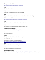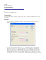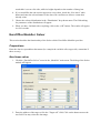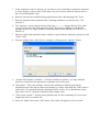
1
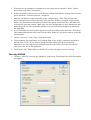
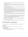
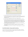
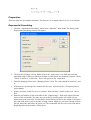
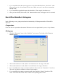
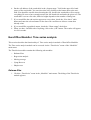
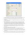
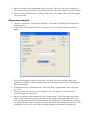
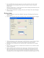
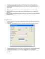
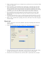
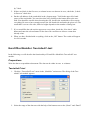
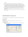
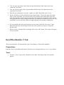
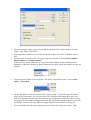
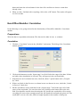
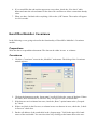
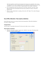
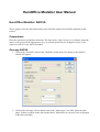
EuroOffice Modeller User Manual
EuroOffice Modeller: ANOVA
We are going to describe the functionality of the ANOVA module of EuroOffice Modeller in this
section.
Preparations
Enter the data into a spreadsheet document. The data can be either in rows or in columns. Input the
names of the groups in the appropriate rows (or columns if the data are arranged in rows) if you
want to use the two-way ANOVA method.
One-way ANOVA
1. Click on the „ANOVA” menu in the „Modeller” main menu. The dialog of the ANOVA
module will appear:
2. Click on the cell range selector button next to the „Input range” text field. Select the data
range. If there are labels in the data set then those should also be selected. These will appear
in the end result table.
3. If the data are not arranged in columns but in rows then please check the „Rows” option
button next to the label „Grouped by:”.
4. If there are labels in the first row (or in the first column if the data are arranged in rows) then
please check the “Labels in first row” check-box.
5. Enter the cell address of the result table in the „Output range:” field. This will mark the
upper left-hand corner of the result table. You may also do this by using the range selector
button. You should be careful when you choose the output cell because the result table will
overwrite the previous content . Make sure you have enough space to the left-hand side and
under the given cell. The result table will be seven cell wide and its height will depend on
the input data.
6. If you would like the end result to appear on a new sheet then please check the „New sheet”
radio button and enter the select name for the sheet. Make sure you do not choose an already
existing name.
7. Choose „One-way” in the „Type” drop-down menu .
8. You can change the significance level with the help of the „Alpha” parameter which has a
default value of 0.05. If you want to change this then either enter the selected value
manually or use the range selector button next to the text field to select the cell with the
value you want use for this parameter.
9. Click on the „OK” button after you finish. The results will appear in a few seconds.
Two-way ANOVA
1. Click the „ANOVA” menu in the „Modeller” main menu. The dialog of the ANOVA module
will appear.
2. Select the „Two-way” option in the „Type” drop-down menu. This will have some extra
dialog elements appear.
3. Click on the range selector button next to the „Input range” text field and select the input
data range. If there are labels, too, then those should also be selected. These will appear in
the end result table.
4. If the data are not arranged by columns, but by rows, then check the „Rows” option button
next to the „Grouped by:” label.
5. If there are labels in the first row (or in the first column if your data are arranged by rows)
then check the „Labels in first row” check-box.
6. Enter the cell address of the result table in the „Output range:” field. This will be the upper
left-hand corner of the result table. You can also select this by the range selector button next
to the text-field. You should be careful when you choose the output cell because the result
table will overwrite the content of the cells . Make sure you have enough space to the lefthand side of the chosen output cell and below it. The result table will be seven cell wide and
its height will depend on the input data.
7. If you would like the end result to appear on a new sheet then check the „New sheet” radio
button and enter the selected sheet name. Make sure you do not choose an already existing
name.
8. You may change the significance level with the help of the „Alpha” parameter which has a
default value of 0.05. If you want to change this then either enter the selected value
manually or use the range selector button next to the text field.
9. You may select the cells that contain the group names with the help of the range selector
button next to the „Groups” text-field.
10. Enter the sample size in the „Sample size” text-field or select the cell containing the value
for this with the range selector button.
11. Click on the „OK” button when you finish. The results will appear in a few seconds.
EuroOffice Modeller: One-Sample Z-test
This section describes how to use the One-Sample Z-test module of EuroOffice Modeller.
Preparation
Enter the data in a spreadsheet document. The data can either be in rows or columns.
One-Sample Z-test
1. Click on the „One-Sample Z-test” menu in the „Modeller” main menu. The dialog of the
One-Sample Z-test module will appear.
2. Click on the button next to the „Data” text field and select the data range.
3. You must enter the significance level of the test in the “Alpha” text-field. You may also use
the range selector button to point at a spreadsheet cell which contains the alpha value. The
default value is 0.05.
4. You must enter the expectation value of the test in the “Mean” text-field.
5. You must enter the standard deviation of the test in the “Standard deviation” text-field.
6. Enter the cell address of the result table in the „Output range:” field in the upper left- hand
corner of the result table. You may also select this by clicking on the cell range selector
button next to the text-field. You should be careful when you choose the output area because
the result table will overwrite the previous content. Make sure you have enough room to the
left- hand side and below the given cell. The result table will be seven cells wide and its
height will depend on the number of data given.
7. If you would like the end result to appear on a new sheet then check the „New sheet” radio
button and enter the desired name for the sheet. Make sure you do not use an already
existing name..
8. After you finish, please click on the „OK” button. The results will appear in a few seconds.
EuroOffice Modeller: Exponential Smoothing
This section describes the functionality of the Exponential Smoothing module of EuroOffice
Modeller. You may perform exponential smoothing on a data series with the help of this module.
The recursive equations defining the method are:
Preparation
Enter the data in a spreadsheet document. The data can be arranged either in rows or in columns.
Exponential Smoothing
1. Click the „Exponential smoothing” menu in the „Modeller” main menu. The dialog of the
Exponential Smoothing module will appear.
2. Click on the cell range selector button next to the „Input range” text field and select the
input data range. If there are labels in the data set then those also should be selected. Check
“Labels in first row” in this case. These will appear in the result table.
3. Enter the damping factor in the “Damping factor” field. The value should be between 1 and
0.
4. If the data are not arranged by columns, but by rows, then check the „ Grouped by Rows”
option button.
5. If there are labels in the first row, or columns, then check the „Labels in first row” checkbox.
6. Enter the cell address of the result table in the „Output range:” field in the upper left-hand
corner of the result table. You may also select this by clicking on the cell range selector
button next to the text-field. You should be careful when you choose the output cell because
the result table will overwrite already existing content. Make sure you have enough room to
the left- hand side and below the given cell. The result table will be seven cells wide and its
height depends on the number of data given.
7. If you would like the end result to appear on a new sheet then check the „New sheet” radio
button and enter the selected name for the sheet. Make sure you do not chosse a name that
already exists.
8. If you would like a graphical output then check the “Chart output” check-box, too.
9. After you have finish, click on the „OK” button and the results will appear in a few seconds.
EuroOffice Modeller: Histogram
In the following we are going to describe the functionality of Histogram module of EuroOffice
Modeller.
Preparation
Enter the data in a spreadsheet document. The data can be arranged either by rows or by columns.
Histogram
1. Click the „Histogram” menu in the „Modeller” main menu. The dialog of the Histogram
module appears.
2. Click on the button next to the „Data” text field. Select the the range of the data.
3. Click on the button next to the „Bins” text field. Select the range of the bins.
4. If you would like the output to contain cumulative data, check the “Cumulative” check-box.
The result will be the cumulative column in percentages.
5. If you would like the output to contain sorted data, check the “Sorted” check-box. The
result will contain the sorted values with the corresponding bins in order.
6. Put the cell address of the result table in the „Output range:” field in the upper left- hand
corner of the result table. You can also select it by clicking on the button next to the textfield. You should be careful when choosing the cell, because the result table will overwrite
everything. Be sure to have enough room to the left- hand side and under the given cell. The
result table is seven cells wide, while its height depends on the number of data given..
7. If you would like the end result to appear on a new sheet, check the „New sheet” radio
button and enter the selected name for the sheet. Be careful not to choose a name that
already exists.
8. If you would like a graphical output, check the “Chart output” check-box.
9. When you have finished with everything, click on the „OK” button. The results will appear
in a few seconds.
EuroOffice Modeller: Time series analysis
This section describes the functionality of Time series analysis module of EuroOffice Modeller.
The Time series analysis module can be accessed via the “TimeSeries” menu of the “Modeller”
main menu.
The TimeSeries module contains the following sub-modules:
– Kalman-filter
– Regression analysis
– Moving average
– Ljung-Box test
– Shapiro-test
Kalman-filter
1. Click the „TimeSeries” menu in the „Modeller” main menu. The dialog of the TimeSeries
module appears.
2. Click on the button next to the „Input range” text field. Select the range of the data. If there
are labels, those should also be selected. They will appear in the end result table.
3. If the data are not in columns but rows, check the „Rows” option button at the „Grouped
by:” label.
4. If there are labels in the first row, or column in case our data are in rows, check the „Labels
in first row” check-box.
5. Put the cell address of the result table in the „Output range:” field in the upper left- hand
corner of the result table. You can also select it by clicking on the button next to the textfield. You should be careful when choosing the cell, because the result table will overwrite
everything. Be sure to have enough room to the left- hand side and under the given cell. The
result table is seven cells wide, while its height depends on the number of data given.
6. If you would like the end result to appear on a new sheet, check the „New sheet” radio
button and enter the selected name for the sheet. Be careful not to choose a name that
already exists.
7. In the „Type” drop-down menu choose „Kalman”.
8. Put the estimate of the filter in the “Filter estimate” field. You enter it manually or click on
the button next to the text-field and select the cell which contains the selected value.
9. Put in the estimate of the measurement in the “Measure estimate” field. You can either enter
it manually or click on the button next to the text-field and select the cell which contains the
selected value.
10. Put the estimate of the error in the “Error estimate” filed. You can enter it manually or click
on the button next to the text-field and select the cell which contains the selected value.
11. Put the precision of the computation in the “Precision” filed. You can enter it manually or
click on the button next to the text-field and select the cell which contains the selected value.
12. When you have finished with everything, click on the „OK” button. The results will appear
in a few seconds.
Regression analysis
1. Click the „TimeSeries” menu in the „Modeller” main menu. The dialog of the TimeSeries
module appears.
2. In the „Type” drop-down menu chose „Regression”. Extra dialog elements are going to
appear.
3. Click on the button next to the „Input range” text field. You can select the range of the
explanatory variables. If there are labels, those also should be selected. They will appear in
the end result table.
4. If the data are not in columns but rows, check the „Rows” option button at the „Grouped
by:” label.
5. If there are labels in the first row (or column in case your data are in rows) check the
„Labels in first row” check-box.
6. Put the cell address of the result table in the „Output range:” field in the upper left- hand
corner of the result table. You can also select it by clicking on the button next to the textfield. You should be careful when choosing the cell, because the result table will overwrite
everything. Be sure to have enough room to the left- hand side and under the given cell. The
result table is seven cells wide, while its height depends on the number of data given.
7. If you would like the end result to appear on a new sheet, check the „New sheet” radio
button and enter the selected name for the sheet. Be careful not to choose a name that
already exists!
Enter the Y ranges in the “Y” field. You can also do this by clicking on the button next to the
text-field and select the chosen cell range.
8. When you have finished with everything, click on the „OK” button. The results will appear
in a few seconds.
Moving average
1. Click the „TimeSeries” menu in the „Modeller” main menu. The dialog of the TimeSeries
module appears.
2. In the „Type” drop-down menu chose „Moving average”. Extra dialog elements will appear.
3. Click on the button next to the „Input range” text field. Select the range of the data. If there
are labels, those should also be selected. They will appear in the end result table.
4. If the data are not in columns but rows, check the „Rows” option button at the „Grouped
by:” label.
5. If there are labels in the first row, or column in case our data are in rows, check the „Labels
in first row” check-box.
6. Put the cell address of the result table in the „Output range:” field in the upper left- hand
corner of the result table. You can also select it by clicking on the button next to the textfield. You should be careful when choosing the cell, because the result table will overwrite
everything. Be sure to have enough room to the left- hand side and under the given cell. The
result table is seven cells wide, while its height depends on the number of data given.
7. If you would like the end result to appear on a new sheet, check the „New sheet” radio
button and enter the selected name for the sheet. Be careful not to choose a name that
already exists.
8. In the “Type” drop-down menu you can choose if you would like to calculate mean
(default) or sum.
9. Put the period for which the moving average should be calculated in the “Window size”
text-field.
10. When you have finished with everything, click on the „OK” button. The results will appear
in a few seconds.
Ljung-Box test
1. Click the „TimeSeries” menu in the „Modeller” main menu. The dialog of the TimeSeries
module appears.
2. In the „Type” drop-down menu choose „Ljung-Box”. Extra dialog elements will appear.
3. Click on the button next to the „Input range” text field. Select the range of the data. If there
are labels, those also should be selected. They will appear in the end result table.
4. If the data are not in columns but rows, check the „Rows” option button at the „Grouped
by:” label.
5. If there are labels in the first row, or column in case your data are in rows, check the „Labels
in first row” check-box.
6. Put the cell address of the result table in the „Output range:” field in the upper left- hand
corner of the result table. You can also select it by clicking on the button next to the textfield. You should be careful when choosing the cell, because the result table will overwrite
everything. Be sure to have enough room to the left- hand side and under the given cell. The
result table is seven cells wide, while its height depends on the number of data given.
7. If you would like the end result to appear on a new sheet, check the „New sheet” radio
button and enter the selected name for the sheet. Be careful not to choose a name that
already exists.
8. You should enter the number of lags, for which the program should calculate the test in the
“Lag” text-field. If it is zero (default) then the calculation will be done for all possible lags.
9. When you have finished with everything, click on the „OK” button. The results will appear
in a few seconds.
Shapiro-test
1. Click the „TimeSeries” menu in the „Modeller” main menu. The dialog of the TimeSeries
module appears.
2. In the „Type” drop-down menu chose „Shapiro-test”. Extra dialog elements will appear.
3. Click on the button next to the „Input range” text field. Select the range of the data. If there
are labels, those should also be selected. They will appear in the end result table.
4. If the data are not in columns but rows, check the „Rows” option button at the „Grouped
by:” label.
5. If there are labels in the first row, or column in case our data are in rows, check the „Labels
in first row” check-box.
6. Put the cell address of the result table in the „Output range:” field in the upper left- hand
corner of the result table. You can also select it by clicking on the button next to the textfield. You should be careful when choosing the cell, because the result table will overwrite
everything. Be sure to have enough room to the left- hand side and under the given cell. The
result table is seven cells wide, while its height depends on the number of data given.
7. If you would like the end result to appear on a new sheet, check the „New sheet” radio
button and enter the selected name for the sheet. Be careful not to choose a name that
already exists.
8. When you have finished with everything, click on the „OK” button. The results will appear
in a few seconds.
EuroOffice Modeller: Two-tailed F-test
In the following we will describe the functionality of EuroOffice Modeller's Two-tailed F-test
module.
Preparations
Write the data to a spreadsheet document. The data can be either in rows or columns.
Two-tailed F-test
1. Click the „Two-tailed F-test” menu in the „Modeller” main menu. The dialog of the Twotailed F-test module appears.
2. Select the range of the data sets with the help of the buttons next to the „Data1” and “Data2”
text-fields.
3. Enter the test confidence level in the “Alpha” text-field. The default value is 0.05.
4. Put the cell address of the result table in the „Output range:” field in the upper left- hand
corner of the result table. You can also select it by clicking on the button next to the textfield. You should be careful when choosing the cell, because the result table will overwrite
everything. Be sure to have enough room to the left- hand side and under the given cell. The
result table is seven cells wide, while its height depends on the number of data given.
5. If you would like the end result to appear on a new sheet, check the „New sheet” radio
button and enter the selected name for the sheet. Be careful not to choose a name that
already exists.
6. When you have finished with everything, click on the „OK” button. The results will appear
in a few seconds.
EuroOffice Modeller: Chi-square Test
In the following section we are going to describe the functionality of EuroOffice Modeller's Chisquare test module.
Preparations
Write the data to a spreadsheet document. The data can be either in rows or columns.
Chi-square test
1. Click the „Chi-square Test” menu in the „Modeller” main menu. The dialog of the Chisquare test module appears.
2. You can select the range of the observed data with the help of the button next to the
„Observed” text-field.
3. You can select the range of the expected data with the help of the button next to the
„Expected” text-field.
4. Enter the test confidence level in the “Alpha” text-field. The default value is 0.05.
5. Put the cell address of the result table in the „Output range:” field in the upper left- hand
corner of the result table. You can also select it by clicking on the button next to the textfield. You should be careful when choosing the cell, because the result table will overwrite
everything. Be sure to have enough room to the left- hand side and under the given cell. The
result table is seven cells wide, while its height depends on the number of data given.
6. If you would like the end result to appear on a new sheet, check the „New sheet” radio
button and enter the selected name for the sheet. Be careful not to choose a name that
already exists.
7. When you have finished with everything, click on the „OK” button. The results will appear
in a few seconds.
EuroOffice Modeller: T-Test
This section describes the functionality of the T-test module of EuroOffice Modeller.
Preparations
Enter the data in a spreadsheet document. The data can be arranged either by rows or by columns.
T-test
1. Click the „T-test” menu in the „Modeller” main menu. The dialog of the T-test module
appears.
2. You can select the range of the selected data sets with the help of the button next to the
„Data1” and “Data2” text-fields.
3. You can put the confidence level of the test in the “Alpha” text-field . Its default value is
0.05.
4. Enter the type of the this in the “Test type” drop-down menu. It can be Paired samples,
Equal variance or Unequal variance.
In the first case, the two data sets are treated as paired samples. In the second case, the
hypothesis is that the variances of the two data sets are equal, while in the third case they are
unequal.
5. You can enter the mode of the test In the “Test mode” drop-down menu . It can be Onetailed or Two-tailed.
6. Put the cell address of the result table in the „Output range:” field in the upper left- hand
corner of the result table. You can also select it by clicking on the button next to the textfield. You should be careful when choosing the cell, because the result table will overwrite
everything. Be sure to have enough room to the left- hand side and under the given cell. The
result table is seven cells wide, while its height depends on the number of data given.
7. If you would like the end result to appear on a new sheet, check the „New sheet” radio
button and enter the selected name for the sheet. Be careful not to choose a name that
already exists.
8. When you have finished with everything, click on the „OK” button. The results will appear
in a few seconds.
EuroOffice Modeller: Correlation
In the following we are going to describe the functionality of EuroOffice Modeller's Correlation
module.
Preparations
Write the data to a spreadsheet document. The data can be either in rows or columns.
Correlation
1. Click the „Correlation” menu in the „Modeller” main menu. The dialog of the Correlation
module appears.
2. Click on the button next to the „Input range” text field. Select the range of the data. If there
are labels, those should also be selected. They will appear in the end result table.
3. If the data are not in columns but rows, check the „Rows” option button at the „Grouped
by:” label.
4. If there are labels in the first row, or column in case our data are in rows, check the „Labels
in first row” check-box.
5. Put the cell address of the result table in the „Output range:” field in the upper left- hand
corner of the result table. You can also select it by clicking on the button next to the textfield. You should be careful when choosing the cell, because the result table will overwrite
everything. Be sure to have enough room to the left- hand side and under the given cell. The
result table is seven cells wide, while its height depends on the number of data given.
6. If you would like the end result to appear on a new sheet, check the „New sheet” radio
button and enter the selected name for the sheet. Be careful not to chose a name that already
exists.
7. When you have finished with everything, click on the „OK” button. The results will appear
in a few seconds.
EuroOffice Modeller: Covariance
In the following we are going to describe the functionality of EuroOffice Modeller's Covariance
module.
Preparations
Write the data to a spreadsheet document. The data can be either in rows or columns.
Covariance
1. Click the „Covariance” menu in the „Modeller” main menu. The dialog of the Covariance
module appears.
2. Click on the button next to the „Input range” text field. Select the range of the data. If there
are labels, those should also be selected. They will appear in the end result table.
3. If the data are not in columns but rows, check the „Rows” option button at the „Grouped
by:” label.
4. If there are labels in the first row, or column in case our data are in rows, check the „Labels
in first row” check-box.
5. Put the cell address of the result table in the „Output range:” field in the upper left- hand
corner of the result table. You can also select it by clicking on the button next to the text-
field. You should be careful when choosing the cell, because the result table will overwrite
everything. Be sure to have enough room to the left- hand side and under the given cell. The
result table is seven cells wide, while its height depends on the number of data given.
6. If you would like the end result to appear on a new sheet, check the „New sheet” radio
button and enter the selected name for the sheet. Be careful not to choose a name that
already exists.
7. When you have finished with everything, click on the „OK” button. The results will appear
in a few seconds.
EuroOffice Modeller: Descriptive statistics
In the following section we are going to describe the functionality of EuroOffice Modeller's
Descriptive statistics module.
Preparations
Write the data to a spreadsheet document. The data can be either in rows or columns.
Descriptive statistics
1. Click the „Descriptive statistics” menu in the „Modeller” main menu. The dialog of the
Descriptive statistics module appears.
2. Click on the button next to the „Input range” text field. Select the range of the data. If there
are labels, those should also be selected. They will appear in the end result table.
3. If the data are not in columns but rows, check the „Rows” option button at the „Grouped
by:” label.
4. If there are labels in the first row, or column in case our data are in rows, check the „Labels
in first row” check-box.
5. Put the cell address of the result table in the „Output range:” field in the upper left- hand
corner of the result table. You can also select it by clicking on the button next to the textfield. You should be careful when choosing the cell, because the result table will overwrite
everything. Be sure to have enough room to the left- hand side and under the given cell. The
result table is seven cells wide, while its height depends on the number of data given.
6. If you would like the end result to appear on a new sheet, check the „New sheet” radio
button and enter the selected name for the sheet. Be careful not to choose a name that
already exists.
7. If you would like to change the confidence interval for the mean, check the check-box
“Confidence level for mean” and enter the selected value (the default value is 0.95).
8. If you would like to set the k-th largest value manually, check the “Kth largest” check-box
and enter the selected value.
9. If you would like to set the k-th smallest value manually, check the “Kth smallest” checkbox and enter the selected value.
10. When you have finished with everything, click on the „OK” button. The results will appear
in a few seconds.
EuroOffice Modeller: Random
In the following section we are going to describe the functionality of EuroOffice Modeller's
Random module. With the help of this module you can generate random numbers of different
distributions. The distributions implemented are the following:
Beta-distribution
http://en.wikipedia.org/wiki/Beta_distribution
Alpha, Beta
The shape parameters of the distribution. Both should be non-negative real numbers.
Binomial distribution
http://en.wikipedia.org/wiki/Binomial_distribution
n
Number of trials, which should be an integer.
p
The success probability in each trial, which should be a real number between 0 and 1.
Chi-square distribution
http://en.wikipedia.org/wiki/Chi-squared_distribution
df
The degrees of freedom which should be an integer greater then zero.
Custom distribution
Create your own distribution by giving the values of the set and their probabilities.
Variables
The variables are the values from which you choose.
Probabilities
The probabilities for each value should sum up to 1.
Dirichlet distribution
http://en.wikipedia.org/wiki/Dirichlet_distribution
Alpha
Concentration parameters (vector); each should be greater then zero.
Exponential distribution
http://en.wikipedia.org/wiki/Exponential_distribution
Lambda
The rate/inverse scale parameter, which should be greater then zero.
F-distribution
http://en.wikipedia.org/wiki/F-distribution
df (numerator)
The degrees of freedom in the numerator which can be an arbitrary positive real number.
df (denominator)
The degrees of freedom in the denominator which can be an arbitrary positive real number.
Gamma distribution
http://en.wikipedia.org/wiki/Gamma_distribution
Shape
The shape parameter, which should be a positive real number.
Scale
The scale parameter, which should be a positive real number.
Geometric distribution
http://en.wikipedia.org/wiki/Geometric_distribution
p
The success probability, which should be between 0 and 1.
Gumbel distribution
http://en.wikipedia.org/wiki/Gumbel_distribution
Location
The location parameter.
Scale
The scale parameter, which should be a positive real number.
Hypergeometric distribution
http://en.wikipedia.org/wiki/Hypergeometric_distribution
n
The number of successful draws.
m
The number of unsuccessful draws.
N
The number of items sampled should be less than n+m.
Laplace distribution
http://en.wikipedia.org/wiki/Laplace_distribution
Location
The location parameter.
Scale
The scale parameter, which should be a positive real number.
Logistic distribution
http://en.wikipedia.org/wiki/Logistic_distribution
Location
The location parameter.
Scale
The scale parameter, which should be a positive real number.
Log-normal distribution
http://en.wikipedia.org/wiki/Log-normal_distribution
Mean
The mean of the distribution.
Sigma
The standard deviation of the distribution, which should be a positive real number.
Logarithmic Series distribution
Also known as the logarithmic distribution or log-series distribution.
http://en.wikipedia.org/wiki/Logarithmic_distribution
p
The success probability, which should be between 0 and 1.
Multinomial distribution
http://en.wikipedia.org/wiki/Multinomial_distribution
Experiments
The number of trials.
Probabilities
A vector containing the event probabilities, which should sum up to 1.
Multivariate Normal distribution
http://en.wikipedia.org/wiki/Multivariate_normal_distribution
Mean
The mean vector of the distribution.
Covariance
The covariance matrix of the distribution. If the mean vector has n elements, it should be a n times n
positive definite matrix.
Negative Binomial distribution
http://en.wikipedia.org/wiki/Negative_binomial_distribution
n
The Number of trials, which should be an integer.
p
The success probability in each trial. This should be a real number between 0 and 1.
Non-central Chi-square distribution
http://en.wikipedia.org/wiki/Noncentral_chi-squared_distribution
df
The degrees of freedom, which should be an integer greater then zero.
Non-centrality
The non-centrality parameter, which should be greater then zero.
Non-central F distribution
http://en.wikipedia.org/wiki/Noncentral_F-distribution
df (numerator)
The degrees of freedom in the numerator, which can be arbitrary positive real number.
df (denominator)
The degrees of freedom in the denominator, which can be arbitrary positive real number.
Non-centrality
The non-centrality parameter, which should be greater then zero.
Normal distribution
http://en.wikipedia.org/wiki/Normal_distribution
Mean
The mean of the distribution.
Sigma
The standard deviation of the distribution, which should be greater then zero.
Pareto distribution
Draw samples from a Pareto II or Lomax distribution.
http://en.wikipedia.org/wiki/Lomax_distribution
Shape
The shape parameter of the distribution, which should be greater then zero.
Poisson distribution
http://en.wikipedia.org/wiki/Poisson_distribution
Lambda
The lambda parameter of the distribution, which should be greater then zero.
Power distribution
Draws samples in [0, 1] from a power distribution with positive exponent a - 1. Also known as the
power function distribution. Link to the numpy function.
a
The parameter of the distribution, which should be greater then zero.
Uniform random integers
http://en.wikipedia.org/wiki/Uniform_distribution_(discrete)
Low
The minimum of the interval where the samples are drawn from.
High
The maximum of the interval where the samples are drawn from.
Rayleigh distribution
http://en.wikipedia.org/wiki/Rayleigh_distribution
Scale
The scale parameter of the distribution should be non-negative.
Standard Cauchy distribution
http://en.wikipedia.org/wiki/Cauchy_distribution. The standard Cauchy-distribution sets the mean
to 0 and the scale 1.
Standard T-distribution
http://en.wikipedia.org/wiki/Student's_t-distribution
df
The degrees of freedom should be positive.
Triangular distribution
http://en.wikipedia.org/wiki/Triangular_distribution
Low
The value of Lower limit.
High
Upper limit. It should be greater than the value of Low.
Mode
The peak of the distribution should be between value of Low and the value of High.
Uniform distribution
http://en.wikipedia.org/wiki/Uniform_distribution_(continuous)
Low
The minimum of the interval where the samples are drawn from.
High
The maximum of the interval where the samples are drawn from.
von Mises distribution
http://en.wikipedia.org/wiki/Von_Mises_distribution
Mu
The location parameter.
Kappa
The dispersion of the distribution should be non-negative.
Wald distribution
Also known as the inverse Gaussian distribution.
http://en.wikipedia.org/wiki/Inverse_Gaussian_distribution
Mean
The mean of the distribution should be positive.
Scale
The shape of the distribution should be positive.
Weibull distribution
The general Weibull distribution: http://en.wikipedia.org/wiki/Weibull_distribution In this case, the
scale parameter is 1.
Shape
The shape parameter.
Zipf distribution
http://mathworld.wolfram.com/ZipfDistribution.html
a
The parameter of the distribution.
Preparations
Open a new spreadsheet document. You are going to find the parameters of the distribution in the
spreadsheet.
Random
1. Click the „Random” menu in the „Modeller” main menu, after which the dialog of the
Random module appears.
2. Give the sample size in the “Sample size” field. You may also do this by clicking on the
button next to this text-field. Then you may select the cell containing the selected value.
3. Put the cell address of the result table in the „Output range:” field in the upper left- hand
corner of the result table. You can also select it by clicking on the button next to the textfield. You should be careful when choosing the cell, because the result table will overwrite
everything. Be sure to have enough room to the left- hand side and under the given cell. The
result table is seven cells wide, while its height depends on the number of data given.
4. If you would like the end result to appear on a new sheet, check the „New sheet” radio
button and enter the selected name for the sheet. Be careful not to choose a name that
already exists.
5. Choose the selected distribution in the “Distribution” drop-down menu. The fields asking
for parameters of the distribution will appear.
6. When you have finished with everything, click on the „OK” button. The results will appear
in a few seconds.
EuroOffice Modeller: Solver
This section describes the functionality of the Solver which EuroOffice Modeller provides.
Preparations
Enter the data in a spreadsheet document (for example the variable cells, target cells, constraints if
there are any).
Non-linear solver
1. Click the „EuroOffice Solver” menu in the „Modeller” main menu. The dialog of the Solver
module will appear.
2. Enter the address of the target cell in the “Target cell” field. Click on the button next to the
text field. You may select the data range.
3. In the “Optimize result to” options you can choose if you would like to minimize, maximize
or set the target to a given value. In the latter case you can enter either the chosen value or
the cell referencing that value.
4. Enter the cells that are modified during optimization in the “By changing cells” field .
5. Enter the formula of the constraint in the “Limiting conditions” on the left side (“Cell
reference”).
6. The “Operator” can be chosen to be the following: <=, =, >=, Integer, Binary. If the latter
two are chosen, the Value field should be empty. The Integer conditions mean that the
variables set here are integer numbers, while the Binary means that they are TRUE (1) or
FALSE (0).
7. Enter the value which should be larger, smaller or equal with the constraint expression in the
“Value” field.
8. You may change some of the Solver's settings by clicking on the “Options” button.
9. “Assume Non-Negative Variables” - If all the variables are positive, you may click this
check-box. In this case the appropriate constraints are not necessary.
10. “Error limit” - This is the tolerance value for the calculation, which means that the
calculation stops if the target cell does not change by a larger value than this. If this value is
small, there is no guarantee that the calculation will be correct. If you find that the result
may not be correct, repeat the calculation with a higher value.
11. “Time-out in seconds” - Solving some problems may be time-consuming. If it is too slow,
change this value to a smaller one.
12. After you finish, click on the „OK” button. The results will appear in a few seconds.