Download Polar Qualification System Evaluation Software User's Manual

PQS32
Polar Qualification System
Evaluation Software
Version 1.40
User's Manual
Copyright METRIKA, Hungary
2001
List of contents
1. Introduction .................................................................................................................................3
2. Getting started .............................................................................................................................3
2.1. Installation .............................................................................................................................3
2.2. Password protection...............................................................................................................3
2.3. Registration ...........................................................................................................................3
3. User interface ..............................................................................................................................4
3.1. Menu bar................................................................................................................................4
3.2. Tool bar .................................................................................................................................4
3.3. Status bar ...............................................................................................................................5
3.4. Pop-up menus ........................................................................................................................5
3.5. General properties of the windows........................................................................................5
3.6. Spectrum window ..................................................................................................................7
4. Description of menu commands..................................................................................................8
4.1. File menu ...............................................................................................................................8
4.2. Edit menu...............................................................................................................................12
4.3. Settings menu ........................................................................................................................14
4.4. Arithmetic menu ....................................................................................................................18
4.5. Transform menu ....................................................................................................................19
4.6. Evaluate menu .......................................................................................................................22
4.7. Window menu........................................................................................................................28
5. Operation.....................................................................................................................................29
2
1. Introduction
Welcome as a PQS32 user! We hope that you will be familiar with the PQS32 Evaluation
Software soon and it can really make your work with the spectra faster and more effective.
The PQS32 Evaluation Software is a 32-bit, Windows based software with all the advantages of
this operational system. The user-friendly graphic interface makes it possible to handle several
spectra at the same time without any confusion.
We wish you pleasant, useful and successful work with the PQS32 Evaluation Software.
2. Getting started
Before starting the installation of the program, please read the notes below.
2.1. Installation
The PQS32 Evaluation Software can be found on the floppy disk enclosed with this manual. To
install it on the hard disk (drive C) of your computer just run the A:\INSTALL.BAT file.
1. Insert the floppy disk into drive A
2. Change to drive A.
(in DOS mode type A: <Enter>)
3. Run the INSTALL.BAT file
(in DOS mode type INSTALL <Enter>)
During installation, a new directory is created with the name PQS32 on the hard disk, and the
PQS32.EXE program and the PQS32.CFG that contains the registration code are copied into it.
2.2. Password protection
The PQS32 Evaluation Software is password protected. It means that without entering the proper
password after starting the program, you are not allowed to use any functions of the program.
When starting the program the initial picture appears. It is closed automatically after five seconds
or you can close it earlier by clicking with the mouse or pressing any key on the keyboard. Then
the password dialog window appears where you can type your password. You cannot see what you
type, only <*> characters appear showing how many characters you have already entered. If you
have typed your password, press <Enter> or the <OK> button. If the password is wrong, you get a
warning message and then you can try to type the password again or by pressing the <Exit> button
or the <Escape> key you can quit the program.
If you have passed the password test, you have the possibility to change the password if you feel it
is necessary (see Settings|Change Password).
2.3. Registration
Every PQS32 customer receives a registration code after purchasing the program. This code
should be entered after starting the program for the first time in the registration window (see menu
command Settings|Register). The code consists of 24 characters that contain the identification
string provided by the customer in a coded form. The maximal length of the identification string is
16 characters. This string appears in the top caption of the program during running and on the
3
upper line on any kind of printed page. If there was no registration, instead of the identification
string the 'NOT REGISTERED' message appears.
You should preserve your registration code in any case!
3. User interface
The initial picture shows the name of the program, the version number and the user's identification
string. After a few seconds the main window appears on which the horizontal menu bar on the top
of the screen, the tool bar under the menu bar and the status bar at the bottom of the screen can be
seen.
3.1. Menu bar
The menu titles are in the horizontal menu bar at the top of the screen.
Pressing the left mouse button when the mouse pointer is on a menu title, the title is highlighted
and a vertical submenu, a so-called pull-down menu appears. Submenus contain menu commands
or further submenus. Menu items, which have a small triangle at their right side, activate
additional submenus. The menu command starts a procedure or opens a new window where you
can set certain parameters and/or start procedures. The gray menu items cannot be activated in the
given situation (e.g. file saving is not possible if there is no open file).
Both the keyboard and the mouse can be used to activate a menu command.
When using the keyboard, the underlined character in the names of the menu items is of great
importance. The menu titles can be chosen by pressing the <Alt> key and the appropriate
underlined character at the same time (e.g. press <Alt> + <F> to activate the File menu). Selecting
a menu title, its pull-down menu opens and the list of the menu commands appears. Pressing the
<Escape> button the pull-down menu closes but the menu title remains highlighted. The other
menu titles can be selected by pressing the <left> or the <right> arrow keys. Inside a submenu the
items can be selected by pressing the <up> or the <down> arrow keys. A highlighted menu title or
menu command can be activated either by pressing its underlined character or by pressing the
<Enter> key.
There are some frequently used menu commands which have shortcuts so you can activate them
very quickly by pressing the Ctrl button and an other one at the same time (e.g. File|Open’s
shortcut is Ctrl+O).
The technique of holding the left mouse button pressed and moving the mouse pointer is called
dragging. The mouse should be dragged to the required menu item to select it. When dragging
through a submenu, each active menu item under the mouse pointer is highlighted in turn. The
highlighted item can be activated by releasing the left mouse button on it.
3.2. Tool bar
The tool bar is located under the menu bar and contains the so-called speed buttons. These buttons
makes your work faster because a lot of frequently used menu commands can be activated directly
just by clicking on these buttons by the mouse. The speed button cannot be pressed if the
procedure that belongs to it is not allowed to activate in the given situation (see inactive menu
4
items in the previous chapter 3.1. Menu). The speed buttons and the corresponding menu items or
options are listed below.
File | Open
Settings | Plot Type
File | Save
Settings | Scale
File | Print
Settings | Spectrum Info
File | Print Preview
Settings | Classes
File | Exit
Edit | Cut
Point Method
Edit | Copy
Line Method
Edit | Copy All
Surface Method
Edit | Paste
Edit | Undo
Evaluate | Auto Range Opt.
Edit | Redo
Evaluate | Auto Sequence Opt.
3.3. Status bar
The status bar is located at the bottom of the main window. It displays information about the status
of the current process (e.g. Fourier transformation).
The status bar shows the positions of the two cursors on the spectrum window as well.
3.4. Pop-up menus
The so-called pop-up menus can be activated by pressing the right mouse button in special cases
(e.g. in the spectrum info window to cut, copy and paste the data sheet). They behave just like the
pull-down menus, the difference is that they appear at the position of the mouse pointer so you do
not have to move the mouse pointer up to the menu bar.
3.5. General properties of the windows
A window can be selected by clicking on it with the mouse.
5
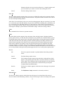
Pressing the icon at the top left corner of a sizable window a pull-down menu appears. You can
select commands to change the size, the position and the state of the window or you can close it.
The position of the window can be modified by picking it up (at the top horizontal title bar) and
dragging it with the mouse. If the window is sizable, its size can be changed by picking up its
frame and dragging it. The state of the window can be set either by the appropriate menu
command or by the buttons described below. These buttons are located at the top right corner of
the window.
Minimized
It shrinks the window into an icon on the Windows desktop.
Maximized
It sets the size of the window to its maximum value i.e. the window fills up the whole screen area.
Normal
It returns the window to its previous size before it was maximized or minimized. This button
appears instead of the minimized or maximized button depending on the current state of the
window. In normal state the window does not fill up the whole screen area so you can easily
activate other visible windows just by clicking on them by the mouse.
Close
The window can be closed by clicking on the button at the top right corner or by pressing the
<Alt> + <F4> keys at the same time or in most cases pressing the Cancel or the Close button or
the <Esc> key also works.
In most cases there are graphic components in the window which you can select either by clicking
on them with the mouse or by pressing the <Tab> key. There is a so-called Tab order defined that
determines the selection order of the components if you press the <Tab> key. In some cases the
arrow buttons can also be used to change the selection (e.g. select another button). Pressing the
<Enter> key, the selected button is pressed. If not a button type component is selected, then if you
press the <Enter> key, the default button is 'pressed'. The default button has a little bit stronger
shadow than the other buttons have. The default button is usually the OK button. If a component is
selected, there is a dotted line frame around the caption of it or the text of the component is
highlighted. The most frequently used graphic components are described below.
Button
Click on it.
Option buttons
Click on the required choice.
6
Check box
Click on the check box to alter the state of it.
Edit box
Click on the edit box and edit the text.
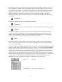
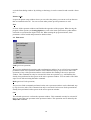
List box
Select the required item by clicking on it with
the mouse. Click the small arrows or drag the
slider to see the other list items. The up and
down arrow keys can be used as well.
Combo box
Click the small arrow to see the item list and
select one of the items by clicking on it.
3.6. Spectrum window
The spectrum window contains the plot of the spectra. In case of spectra with ‘GFF’ extension
(see below) the scales of the plot cannot be re-scaled. In other cases the scale of the plot can be
changed by the buttons at the right side as well as at the bottom of the plot or by activating the
Settings|Scale menu command.
Pressing the small arrows at the plot corners both the x and y-axes
can be re-scaled according to the directions of the arrows.
Pressing this button at the middle of the right side of the plot, the
maximum and the automatic scale alternate.
Pressing the rectangle button located under the previous button on the
right side of the plot, a rectangle-shaped region can be selected in the
plot by the mouse (during area selection keep the left mouse button
pressed).
There are two cursor lines in the plot. Depending on the plot type (see Settings|Plot Type below)
there are two vertical lines or there are a vertical line and a horizontal one.
The cursors can be moved with the mouse after catching either of them with the mouse pointer
pressing the left mouse button or by the left and right arrow keys on the keyboard (arrow keys
only available if not polar scale is used!). If you just use the arrow keys, you can move the one
cursor, if you press the Shift button and use the arrow keys at the same time, you can move the
other cursor. The current cursor line positions are always displayed in the status bar. The cursor
positions can also be set in the Manual Range Optimization window by entering the x axis value in
the proper edit boxes (see Evaluate|Range Optimization|Manual).
7
There may be several spectrum windows in the main window at the same time but only one of
them is selected. This is the so-called active spectrum window. The spectrum window always has
a selected spectrum, the active spectrum. It is illustrated with different color by default. A
spectrum from the spectra in the spectrum window can be selected in the Spectrum Info window
(see Settings|Spectrum Info) or by clicking on the curve of the spectrum. If the mouse pointer
does not move for at least half a second on the plot area, the name of the closest spectrum is
displayed at the mouse position.
4. Description of menu commands
Activating the menu commands below either a dialog window appears or a procedure is performed
immediately.
4.1. File menu
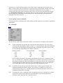
The file formats, which can be used in the software, are listed below according to the extension:
DA
It may contain not only one but also several spectra. Each consists of 350, 650, 700 or
1050 spectrum data (number length is 4 bytes i.e. 7 significant digits) plus some additional
information. The data belong to the 400-2498 nm wavelength range with 2 nm step. The
wavelength ranges depending on the number of data are:
Number of Data
350
650
700
1050
First wavelength
400
600
1100
400
Last wavelength
1098
1898
2498
2498
It is an original file format. The length of the filename may be even 10 characters before
the ‘.da’ extension It is compatible with the DAC file format. If you start the software with
the /DAID command line option, the default scale of the plot will show the corresponding
wavelength range not always the whole DA wavelength range. In this case the different
wavelength range DA files will not be compatible with each other any more.
DAC
It contains only one DA type spectrum and the PQS32 software specific header with
additional information (sample, operator, class, subclass, comment, list of processes,
selected and zero ranges etc.). This file format is generated by the PQS32 software. It is
compatible with the DA file format.
LST
It contains the x and y coordinates of the selected spectrum in two columns. It is a simple
list file that contains ASCII characters. This file format is generated by the PQS32
software as data export file and it cannot be loaded.
8
GFF
It is a general file format. The user defines the number of points (max. 24), the x-axis
scale (first point, difference between points), the x axis label and the unit of measurement.
The number size is 4 bytes i.e. there are 7 significant digits. There may be a comment up
to 20 characters to describe the data point. It is located after the given value. The PQS32
software saves the GFF files with the PQS32 software specific header (see at DA file
format above). GFF files are compatible with the other GFF files if the number of points
and the x-axis scale (first point and difference) are the same. GFF files can be created
either by the PQS32 software (Edit|Edit Spectrum) or manually with any text editor
software. The following example shows how to edit a GFF file:
DATA
6
200
200
Frequency
Hz
0.3456521
0.6321548
0.8567932
0.9629783
0.9415394
0.8703517
{It shows that there is no PQS32 software specific header}
{number of points}
{first point on the x axis}
{difference between points on the x axis}
{x axis label}
{unit of measurement, the x axis label is: Frequency [Hz]}
{1. Impedance value at 200 Hz}
{2. Impedance value at 400 Hz}
{3. Impedance value at 600 Hz}
{4. Impedance value at 800 Hz}
{5. Impedance value at 1000 Hz}
{6. Impedance value at 1200 Hz}
SPE
It consists of 750 spectrum data (number length is 6 bytes i.e. 11 significant digits) so the
length of the file is always 4500 bytes. The data belong to the 1000-2498 nm wavelength
range with 2 nm step. It is an original file format. It is compatible with the SPT file
format.
SPC
This is a general file format (Galactic). Since the PQS32 Evaluation Software uses spectra
with evenly spaced X data only, spectra with non-evenly spaced X data are not supported
(not loaded). The PQS32 Evaluation Software can handle the different types of SPC
spectra but only compatible spectra with the same X data can be loaded or copied into the
same spectra window. Multiple SPC file can be generated by saving all the spectra in a
spectrum window into one file (Save All command with Multiple option).
SPT
It contains an SPE type spectrum and the PQS32 software specific header (see at DA file
format above). This file format is generated by the PQS32 software. It is compatible with
the SPE file format.
TE
It may contain not only one but also several spectra. Each consists of 100 spectrum data (5
significant digits) plus some additional information (e.g. chemical data). The data belong
to the 800-1097 nm wavelength range with 3 nm step. It is an original file format. The TE
spectra can be saved as TEC files one by one.
TECIt contains a TE type spectrum and the PQS32 software specific header (see at DA file format
above). This file format is generated by the PQS32 software. It is compatible with the TE
file format.
NOR
It contains only measured data points written after each other. It is only an input file
format, the loaded data can be saved in GFF format (see above). The NOR files can only
be loaded in the Edit Spectrum window (see its description below) after pressing the Open
button.
9
TXT
This file format is used to load user defined spectra i.e. spectra with different number of
data and with different wavelength ranges and steps. It contains the x and y axis values of
one or more spectra. The first column represents the values of the x-axis while the other
columns contain the y axis values of the spectra. The first line of the TXT file contains the
names of the spectra above the y values. These names become the default file names when
saving the spectra. During loading the lines, which do not contain the x and the y values,
are skipped automatically. When saving a TXT file, the data of the active spectrum and
the PQS32 software specific header (see at DA file format above) is saved in it. The
already saved TXT file contains only one spectrum and it has not the same file format as a
simple TXT file. The PQS32 operating software can open both types of TXT files i.e. the
original, simple list file and the one with the header information and the compressed
spectrum data.
Open
The Open dialog window appears where you can set the necessary path (drive combo box and
directory list box) and filter (filter combo box) that determines the file extension. The extensions
may be ‘SPE', 'SPT', 'SPC', ‘DA’, ‘DAC’, ‘TE’, ‘TEC’, ‘GFF’ and ‘TXT’. The files located in the
set directory and match the filter, are listed in the file list box on the left side of the window. Not
only one but also several files can be selected at the same time. Click on the filename you want to
select in the file list box. Multiple selection is possible if the <Shift> key (continuous selection) or
the <Ctrl> key (not only continuous selection) is pressed during selection clicks. The selected files
are highlighted. You can select and open any file from the file list by double clicking it with the
mouse.
The number of the selected files is displayed under the Cancel button.
According to the Plot property (Plot option buttons), the selected files are loaded into separate
windows (single plot) or into a common window (multiple plot).
When opening the Open dialog window, the filter is set to the extension (except the ‘TXT’
extension), which was used at the last file opening. Incompatible spectra (i.e. different number of
data) cannot be loaded in the same spectrum window.
Buttons:
OK
The selected files are opened and the Open dialog window closes.
Cancel
The Open dialog window closes.
Save
The Save dialog window appears where you can save the active spectrum into the selected
directory with the selected extension. The path and filter selection is the same as in case of the
Open dialog window. The only difference is the possibility to save data as ASCII list files with
‘LST’ extension. Even if you do not add an extension to the filename or you type not the same
extension as the one in the Filter combo box at the end of the filename, the extension set in the
Filter combo box is used automatically when saving the file.
Buttons:
OK
The selected spectrum from the active spectrum window is saved and the
Save dialog window closes. If a file with the same name as typed as new
10
filename already exists in the selected directory, a warning appears and
you can decide if you want to overwrite the existing file or not.
Cancel
The Save dialog window closes.
Save All
The Save dialog window appears where you can save all the files in the active spectrum window
into the selected directory with the selected extension. The path and filter selection is the same as
in case of the Open dialog window.
If the file to be saved already exists, an overwrite-warning appears and you can select if you want
to overwrite the given file (OK button), the given fil e and all the remaining files (All button), not
to overwrite the given file (Skip button) or to cancel the save all procedure (Cancel button). If
there are more than one SPC spectra in the spectrum window, you can save them into one file by
checking the ‘Multiple’ option instead of the default ‘Single’ in the Save dialog window..
Close
This command closes the active spectrum window.
Print
The Print dialog window appears where the name of the selected printer is displayed and the
printer options can be set. The data sheet information, the gridlines, the comment and the spectra
list and the marks of the spectra (above the quality points) appear on the printed page by default
while the black-and-white, the quality point lines and the quality point ellipse options are not
checked at the beginning. The spectra list, the quality point lines and the quality point ellipse
check boxes cannot be set if there is only one spectrum in the plot to be printed. Even if the
comment checkbox is checked, there is no comment on the printed page if the text field in the
Comment window (see below) is empty. The orientation and the line width as well as the font size
(6-20, 10 by default) of the plot on the printed page can also be set on the printer options panel.
Buttons:
OK
The active spectrum window is printed and the Print dialog window
closes.
Cancel
The Print dialog window closes.
Comment
The Comment window appears where the three comment lines which
appear on the printed page if the Show Comment checkbox is checked
can be edited. The comment of the selected spectrum (see the Spectrum
Info window) can be copied in the Comment field by pressing the
Comment from Data Sheet button.
Preview
The Preview window appears, which shows how the page to be printed
looks like.
Setup
The File|Printer Setup command is activated (see below).
Print Preview
The Preview window appears, which shows how the page to be printed looks like (same as
Preview button in the Print dialog window). The preview image is drawn according to the options
11
set in the Print dialog window. By clicking on the image, it can be zoomed in and out with a factor
of 2.
Printer Setup
It opens the printer setup window where you can select the printer you want to use from the ones
that are installed on the PC. You can set some other printer specific parameters as well.
Exit
It closes all the spectrum windows and finishes the operation of the program. When leaving the
program, all the options (see Setting|Options) as well as the latest open and save paths and the
extension are saved into the PQS32.CFG file. When starting the program next time, these
parameters will be loaded and presented as default values.
4.2. Edit menu
Undo (previous operation)
The previous arithmetical operations and transformations and the Cut as well as Paste commands
performed on the active spectrum window can be eliminated step by step in reverse order. The
operations of any of the spectrum window can be undone after making it the active spectrum
window. This command can only be activated if at least one operation (e.g. Add Number) has
already been performed on the spectra in the active spectrum window. You can undo of the Undo
steps as well with activating the Redo command.
Redo (previous Undo operation)
The previous Undo commands performed on the active spectrum window can be eliminated step
by step in reverse order. This command can only be activated if at least one Undo operation has
already been performed on the spectra in the active spectrum window.
Cut
The selected spectrum is cut from the spectrum window. This command can only be activated if
there are more than one spectrum in the spectrum window. This operation can be deleted by the
Edit|Undo command.
12
Copy
The selected spectrum is copied and stored in the memory. The data of the spectrum are available
on the Clipboard for other Windows applications if the software is registered.
Copy All
All the spectra in the active spectrum window are copied and stored in the memory. The data of
the spectra (up to 32Kb, the number of spectra depends on the spectrum size) are available on the
Clipboard for other Windows applications if the software is registered.
Paste
The last copied spectra (Copy, Copy All) are inserted in the active spectrum window. This
command can only be activated if there are spectra (or at least one spectrum) in the memory,
which has been copied before and are compatible with the spectra, which are in the active
spectrum window. E.g. a spectrum with ‘DA’ extension is not compatible with an ‘SPT’ spectrum
because the wavelength ranges are different. This operation can be deleted by the Edit|Undo
command.
Copy Plot
The Copy Plot dialog window appears, where you can set the parameters of the bitmap to be
copied such as the width (400..1600, 800 by default) and the height (250..1000, 500 by default) in
pixels as well as the font size (6..36, 12 by default). The plot is copied to the Clipboard in order to
use it in other Windows applications. The Clipboard is available only if the software is already
registered.
Duplicate
The whole spectrum window is duplicated with all the spectra, spectra information, selections,
history etc.
Edit Spectrum
The Edit Spectrum dialog window appears where you create or modify spectra with ‘GFF’
extension. If the active spectrum window contains spectra with ‘GFF’ extension, the data of the
selected spectrum appear in the Edit Spectrum window. This way it is very easy to modify its data.
You can specify the filename and the X axis label before creating a new spectrum. The line
number (No.), the possible data description and the value itself can be modified in the given edit
boxes. When clicking on an item in the data list, the edit boxes above the list show the data of the
selected item. When adding, replacing or removing a line at the data list, the position is
determined by the line number (No.).
Buttons:
Create
A new spectrum window is created where the generated or modified data
are the data of the new spectrum. Then the Edit Spectrum dialog window
closes.
Open
The Open dialog window appears where you can set the necessary path
to load a file. The extension is NOR, it cannot be modified. When
loading a NOR file, the software checks if there is a file with the same
name as the selected one but with PAR extension in the given directory.
13
If there is one, it is automatically loaded and the parameters read from it
are written in the Sample and Comment fields of the spectrum (see them
in the Spectrum Info window).
Cancel
Then the Edit Spectrum dialog window closes without any change in the
spectra or generating a new spectrum.
Add
A new line is added to the spectrum data.
Replace
The data of the selected line are replaced with the contents of the edit
boxes.
Remove
The selected line is removed from the data list.
4.3. Settings menu
Plot Type
The Plot Type dialog window appears where you can define how to plot the data of the active
spectrum window. There are four different co-ordinate systems to choose (Wavelength, Wave
number, Angle and Polar). In the first three cases there is a Descartes type coordinate system in
the spectrum window where the intensity is plotted as a function of the wavelength, the wave
number or the calculated angle. In case of ‘GFF’ spectra, there are only two different co-ordinate
systems to choose (Descartes and polar) and the Data Selection option button panel is not visible
because all the spectrum points take part in the evaluation of the quality points. In this case there
are two possibilities to plot the data in the Descartes co-ordinate system, the column diagram and
the traditional line or point curves.
If Polar coordinate system is selected, the Method option buttons panel and the 'Show Quality
Points Only' check box appear in the Plot Type dialog window as well as the Method speed
buttons become visible on the Tool bar. In the polar coordinate system the evaluation method
(Point, Line, Surface) should be set as well and you can do this either in the Method option
buttons panel or by clicking on one of the Method speed buttons on the Tool bar. The quality
points of the spectra are always plotted in the Polar coordinate system. If you want to see them
without the spectrum data, check the 'Quality Points Only' check box. Lines between the quality
points can be drawn to see the order of them by checking the 'Quality Point Lines’ checkbox. If
the 'Quality Point Ellipse’ checkbox is checked, the so-called quality point ellipse is plotted which
shows the deviation region of the quality points if there are at least two quality points in the plot.
More ellipses can be plotted at the same time if the ‘Ellipses by Mark’ checkbox is checked and
there are spectra groups with different marks (e.g. spectra marked ‘a’ and ‘b’). The ‘Ellipses by
Mark’ checkbox can be set only if the 'Quality Point Ellipse’ checkbox is checked.
The ‘Color by Mark’ checkbox makes it possible to plot the spectra and the ellipses and the
corresponding quality point groups with different colors. Pressing the Colors button, the Colors
14
dialog window appears where you can set the color palette. The colors are determined by the socalled RGB numbers i.e. the intensity values of the Red, Green and Blue contents of the given
color. Since the intensity range is 0-255 for all the three basic colors, there are 16777216 possible
colors available in the software. The 16 colors of the palette are listed on the left side of the
window. You can select the index number of the color you would like to modify in the Index
combo box. There are the actual color and the new color drawn in the Color Setting panel.
Changing the Red, Green or Blue content of the new color, it is refreshed automatically. If you
press the OK button in the Color Setting panel, the new color replaces the old one at the selected
index in the color palette. Pressing the Default button in the Color Setting panel, the default colors
are set. Any change in the color palette remains only if you close the Colors window by pressing
the OK button.
The way of data selection can be set in the Data Selection option button panel. There are four
possibilities to select data from the spectra:
All Points
All points of the spectra are plotted even if there are omitted or zero points.
Non-Selected Points are Zeros
All the points are plotted but the ones, which are not selected, are taken into account as
zero points.
Non-Selected Points are Omitted
Only the selected points are plotted, the omitted and the zero points are neglected.
Selected and Zero Points
Only the selected and the zero points are plotted.
You can do the selection automatically or manually, see Evaluate|Range Optimization below.
Scale
The Scale dialog window appears where the scale of the X as well as the Y-axes can be modified.
Buttons:
OK
The active spectrum window is re-scaled according to the current
minimum and maximum values and the Scale dialog window closes.
Cancel
The Scale dialog window closes.
Default
The current scale values are replaced by the default scale values.
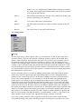
Spectrum Info
The Spectrum Info window appears. The caption shows the caption of the active spectrum
window. There is the Spectra list box on the right side. You can select any of the listed spectra.
After selecting a spectrum, its information data appear on the left side of the window, in the Data
Sheet and in the Comment field as well as its name will be the caption of the active spectrum
window and that of the Spectrum Info window.
15
The Data Sheet consists of several data fields (Sample, Operator, Date, Class, SubClass, Mark)
which you can modify and additional information about the spectrum (quality point coordinates,
number of points). It is indicated if the spectrum has already been processed or not.
The Date field cannot be modified, it shows the date of the original (measured) spectrum.
The Class and Subclass fields are combo boxes so you can select any classes and subclasses which
have been defined in the Class and Subclass dialog window (see Settings|Classes). There is a
possibility to define new classes and subclasses in the Spectrum Info window as well. Type the
name of the new class in the text field of the class combo box and exit the combo box by pressing
the <Tab> key or clicking on an other editable component (e.g. edit box) and the new class is
added to the class list. Do the same at the subclass combo box if you want to define a new
subclass.
Every spectrum has a mark, a string up to three characters. It can be used to group and order the
spectra (see Plot Type Options above and Serial Number button below).
You can type any comments in the Comment field. Pressing the right mouse button on the Data
Sheet or on the Comment field, a pop-up menu appears and you can copy and cut the Data Sheet
as well as the Comment information of the selected spectrum and then paste them into another
spectrum. You can paste the copied information even into all the other spectra in the active
spectrum window (‘Copy Data Sheet/Comment to All’ command). This is especially useful if you
want to give the same mark to a group of spectra e.g. before Automatic Range Optimization. The
procedure consists of the following steps:
-
Load the group of spectra into the same spectrum window.
Write the desired mark into the Mark field of the first spectrum.
Press the right mouse button on the Data Sheet area and activate the Copy Data Sheet
command.
Press the right mouse button again and activate the Paste Data Sheet to All command. The
mark of the first spectrum is copied to the Mark field of the other spectra in one step.
Save the spectra to keep the marks.
If you repeat the above procedure on another group of spectra with a different mark, then you can
load the two groups of spectra into the same spectrum window and do the Automatic Range
Optimization (see Evaluate|Range Optimization|Automatic).
Buttons:
Serial Number
Every spectrum in the Spectra List is given a number in the Mark field
according to the order of the spectra. The Mark is printed near the
quality point and so it helps to identify the quality points on the printed
pages.
File List
There are some processes which need more spectra (e.g. averaging). In
these cases this button can be pressed and the file list window shows
which files took part in the given process.
Operations
If the selected spectrum is processed i.e. at least one process has been
performed on its spectrum data, this button is enabled. Pressing it the
Operations window appears in which all the processes of the spectrum
are listed. This is a kind of history of the spectrum.
16
Classes
The Classes and Subclasses dialog window appears. There you can modify the class and subclass
structure. There are two edit boxes and two list boxes in the window. The classes are listed in the
left list box while the subclasses that belong to the selected class are in the right one. The selected
class and subclass are written in the class and subclass edit boxes above the corresponding list
boxes. The classes and subclasses defined here can be used when filling out the data sheet of the
spectra (see Settings|Spectrum Info).
Buttons:
Add Class
The item in the Class edit box is added to the class list if there is no class
with the same name in the class list box.
Add Subclass
The item in the Subclass edit box is added to the subclass list if there is
no subclass with the same name in the subclass list box.
Remove Class
The item in the Class edit box is deleted from the class list.
Remove Subclass
The item in the Subclass edit box is deleted from the subclass list.
Open
The Open dialog window appears where you can choose which file to
open. The file extension is ‘CLA’ (Classes).
Save
The Save dialog window appears where you can set the path and the
filename to save the classes and the corresponding subclasses data in.
Close
The Classes and Subclasses dialog window closes.
Options
The Options dialog window appears where some important properties of the program can be
modified. You can set the language of the program in the Language combo box. After pressing the
OK button, the program will use the selected language in every string that can be seen on the
screen. The size of the spectrum window can also be set. These values (width and height)
determine the initial size of the new spectrum windows after opening. The size is given in pixels.
There are two other options regarding the illustration. The spectrum data on the polar plain can be
plotted clockwise or contra clockwise. On the other hand there is a possibility to draw line
between the points in the plot. The color palette can be set in the Colors dialog window (Colors
button).
Buttons:
OK
The current options take effect and the Options dialog window closes.
Cancel
The Options dialog window closes.
Colors
The Colors dialog window appears, where the color palette can be set
(see the description of the Colors dialog window above at the Plot Type
item.
Default
The current options are replaced by the default options.
17
Register
The Register dialog window appears where you should type the registration code you received
when purchasing the program. If the registration code is right, the user defined identification string
appears in the title bar of the main window and on all printed pages.
Change Password
The Change Password dialog window appears where you should type the new password. You
should type the new password once more (confirmation) and if the two entered strings are the
same, the old password is replaced by the new one i.e. next time you can only use the program if
you type the new password after starting the program. The maximal length of the password is 16
characters.
4.4. Arithmetic menu
Each arithmetical operation can be deleted by the Edit|Undo command even if it is an irreversible
operation (e.g. Absolute Value).
Basic Operations
There are four different basic operations in the submenu: Add, Subtract, Multiply and Divide.
After choosing one of them, a dialog window appears where you can type the number, the socalled factor, which is used in the basic operation (e.g. it is added to the spectra). The caption of
the window shows the selected operation.
Buttons:
OK
The selected operation is performed with the factor on all the spectra of
the active spectrum window. The only exception is if you select division
and type zero as a factor. In this case the division is not performed.
Cancel
The dialog window closes. No operation is performed.
Spectrum Operations
There are four different spectrum operations in the submenu: Add Spectrum, Subtract Spectrum,
Multiply by Spectrum and Divide by Spectrum. After choosing one of them, a dialog window
appears where you can select the spectrum, which is used in the spectrum operation (e.g. it is
added to the other spectra). The caption of the window shows the selected operation. The Spectra
List contains the available spectra i.e. all spectra of all the spectrum windows. If you select the
first item in the spectra list (Open Spectrum), the Open dialog window appears where you can
select the spectrum for the spectrum operation.
18
Buttons:
OK
The selected operation is performed with the spectrum on all the spectra
of the active spectrum window if the spectra are compatible with each
other. The new values are calculated point by point (e.g. the first point of
the selected spectrum is added to the first points of the spectra in the
active spectrum window, then the second etc.). The only exception is if
you select division and there is a zero value in the selected spectrum. In
this case the division is not performed.
Cancel
The dialog window closes. No operation is performed.
Absolute Value
Every point of the spectra in the spectrum window is replaced with the absolute value of it. This
arithmetical operation is irreversible.
Negative Values Only
Every positive point value of the spectra in the spectrum window is replaced with zero. This
arithmetical operation is irreversible.
Average
The spectra in the spectrum window are replaced by the average spectrum. Its points are
calculated from the points of the original spectra by taking the average of the y axis values at
every x-axis value. This arithmetical operation is irreversible.
This command can only be activated if there are more than one spectrum in the spectrum window.
Standard Deviation
The spectra in the spectrum window are replaced by the standard deviation spectrum. Its points are
calculated from the points of the original spectra by taking the standard deviation of the y axis
values at every x-axis value. This arithmetical operation is irreversible.
This command can only be activated if there are more than one spectrum in the spectrum window.
4.5. Transform menu
Each transformation can be deleted by the Edit|Undo command even if it is an irreversible
operation (e.g. Smooth).
19
Smooth
The smoothing is an irreversible transformation that makes the curve of the spectrum smoother.
There are four different smoothing methods in the submenu: Rectangular, Triangular, SavitskyGoley and Fourier. After choosing one of them, a dialog window appears where you can type the
length of the section (in points) which is the parameter of the first three processes. It defines how
many neighboring points are used in the process. The possible values are in the 3..49 range. The
wavelength range (the so-called gap) that belongs to the section is displayed in the bottom edit
box. In case of Rectangular smoothing, the value of each point is replaced with the average of its
value and the neighboring values. In case of Triangular smoothing there is an additional weight
function in the calculation. The closer the neighboring point is the larger its weight is. In case of
Savitsky-Goley smoothing, the points in the section are weighted with the distance between the
center and the given position in the section raised to the second power. In case of Fourier
smoothing you should type the so-called cut-off frequency. The spectra are Fourier transformed
then the Fourier spectrum data below the cut-off frequency are transformed again with the Inverse
Fourier transformation. This is a kind of low pass filtering. The caption of the window shows the
selected smoothing method.
Buttons:
OK
The selected smoothing process is performed with the spectrum on all
the spectra of the active spectrum window.
Cancel
The Smooth dialog window closes. No transformation is performed.
Derivation
The derivation is an irreversible transformation that emphasizes the fast change in the curve of the
spectrum. There are two kinds of derivation in the submenu: First Derivative and Second
Derivative. After choosing one of them, a dialog window appears where you can type the length of
the section (in points) which is the parameter of the processes just like at smoothing (see
Transform|Smooth). It defines how many neighboring points are used in the process. The
possible values are in the 3..49 range. The wavelength range (gap) that belongs to the section is
displayed in the bottom edit box. In case of the First Derivative, the value of each point is replaced
with the difference of the values measured at both ends of the section divided by the length of the
section. In case of the Second Derivative, the value of each point is replaced with the difference of
the values measured at the center point and the average of the values measured at the end points of
the section divided by the length of the section raised to the second power. The caption of the
window shows the selected derivations.
Buttons:
OK
The selected transformation is performed on all the spectra of the active
spectrum window.
Cancel
The Derivation dialog window closes. No transformation is performed.
Normalization
The normalization is an irreversible transformation that helps to compare different spectra. There
are two kinds of normalization in the submenu: By Subtraction and By Division. After choosing
one of them, a dialog window appears where you can type the base point. The default position of
the base point is the position of the first vertical cursor so you can set it by dragging the cursor or
by typing it in the edit box. The transformations are performed on all spectra in the active
20
spectrum window. In case of subtraction, the value of the spectrum at the base point is subtracted
from the whole spectrum. After normalization by subtraction, all the spectra should have 0 at the
base point. In case of division, the whole spectrum is divided by the value of the spectrum at the
base point. After normalization by division, all the spectra should have 1 at the base point.
Buttons:
OK
The selected transformation is performed on all the spectra of the active
spectrum window.
Cancel
The Normalization dialog window closes. No transformation is
performed.
Fourier Transformation (Inverse Fourier Transformation)
The Fourier transformation can be performed on one spectrum at a time. If there is more than one
spectrum in the active spectrum window, a new window is created and the selected spectrum of
the previous active spectrum window is Fourier transformed. After the transformation the Fourier
spectrum of the spectrum appears in the plot window. In this case instead of the Fourier
transformation menu item, the Inverse Fourier Transformation item appears in the menu.
Activating it the Fourier spectrum - below the cut off frequency - is transformed back to normal
spectrum. The cut off frequency can be set just like the base point (see
Transform|Normalization).
Buttons:
OK
The selected transformation is performed on the selected spectrum of the
active spectrum window.
Cancel
The Fourier Transformation dialog window closes. No transformation is
performed.
MSC1 and MSC2
The MSC (Multiplicative Scatter Correction) dialog window appears where the MSC line of the
spectra can be calculated. You can choose if you want to calculate the MSC line of the spectra in
the active spectrum window (New Straight Line) or you want to replace the MSC line of the
spectra to an already fitted MSC line (e.g. a line of an other group of spectra). You can select the
already fitted line from the Fitted lines combo box if there is at least one and the spectra and the
fitted line are compatible with each other. There is a check box at the bottom of the MSC window.
Check it if you want to see the fitted or used MSC line as a spectrum in the active spectrum
window. There are two different MSC methods built in the software, MSC1 and MSC2. Since the
MSC line is calculated in two different ways, the MSC1 and MSC2 lines of the spectra are not
compatible with each other i.e. you cannot use an already fitted MSC1 line as MSC line for an
MSC2 calculation. The MSC calculation is performed according to the set X axis range. The range
can be set in the Range Selection panel by setting the minimum and the maximum values. The
default values are the current cursor positions. The calculated MSC lines remembers the X axis
range where they were calculated and if you use it as an already fitted line in an MSC1 or MSC2
operation, its X axis range is automatically appears in the Range Selection panel and cannot be
changed.
21
Buttons:
OK
The common MSC line is fitted on the spectra of the active spectrum
window. If an old MSC line is used, the original line of the spectra is
replaced with the selected one.
Cancel
The MSC dialog window closes. No transformation is performed.
Select All
The whole possible X axis range can be selected by pressing this button.
SNV
The SNV (Standard Normal Variate) calculation is performed when activating this menu item.
The result of this transformation is usually similar to the MSC calculations. It also shifts each
spectrum but uses only coefficients to change a spectrum derived from the spectrum alone. For
each spectrum the mean m and the standard deviation s is calculated and the y values the spectrum
are transformed to (y-m)/s at all wavelengths.
NPC
The NPC (Norris Pathlength Correction) calculation is performed when activating this menu item.
The NPC window appears where the parameters of the NPC procedure can be set. After pressing
the OK button, the second derivative spectra of the spectra in the active spectrum window are
calculated according to the set gap range (number of points). Then the so-called normalization or
scaling factor is calculated for each spectrum. This factor is the sum of the absolute values of the
second derivative spectrum in the selected X axis range (The range can be set in the Minimum and
Maximum edit boxes, the default values are the current cursor positions). The normalization is
done by dividing all original or the second derivative spectra (set in the Spectra panel) at each X
axis point by the respective factor. There is a possibility to multiply the spectra by the average
factor to avoid very small numbers (Multiply by average factor check box) and to perform a
normalization by subtraction procedure i.e. an offset correction at the set X axis point
(Normalization by subtraction check box, Base Point edit box).
4.6. Evaluate menu
or
In case of spectra with ‘GFF’ extension, the Sequence Optimization menu item appears in the
Evaluate menu, because the quality point evaluation always uses all the points of these spectra, but
the sequence of the data can be changed to find the optimal evaluation. In case of other spectra
like ‘SPE’ or ‘DA’, there is the range optimization instead of the sequence optimization so the
Range Optimization menu item appears.
Sequence Optimization
There are two kinds of sequence optimization in the submenu: Automatic and Manual. The
automatic sequence optimization can be activated if there are at least two spectra in the active
spectrum window.
22
Automatic Sequence Optimization
In the Automatic Sequence Optimization dialog window you can optimize the sequence of the
data to get maximum distance or normalized distance between two spectra groups. The data
groups are selected according to the marks, which can be set in the two mark combo boxes.
There should be at least two spectra groups with different marks to be able to start the
optimization. The number of spectra in the two spectra groups and the corresponding marks
are located in the Data Groups panel. The marks can be changed in the Spectrum Info
window. If there are less than 5 spectra in any of the data groups, a warning appears before
the optimization starts. In the Options panel you can select the method and the type of
distance (base or normalized) for the calculation. The optimization process searches for the
data sequence where the base distance or the normalized distance between the two spectrum
groups are the largest.
The numbers calculated during the optimization are listed below:
Sequence
The current data sequence.
Distance
The distance between the average quality points of the two spectrum
groups on the quality plane.
Deviation
The standard deviation of the quality point positions of a spectrum
group.
Normalized Distance
The distance divided by the distance plus the deviations of the two
spectrum groups. The maximum value of the normalized distance is 1.
Sensitivity
The distance divided by the sum of the two deviations. The smaller the
deviations are (compared to the distance), the larger the sensitivity is. It
is not calculated at zero deviations.
Buttons:
Optimize
It starts the sequence optimization according to the options and
parameters on the two spectrum groups. The distance, the normalized
distance and if possible the deviations (if more than one spectrum is in
the group) and the sensitivity are calculated in every case. The best
results are displayed continuously during the process in the Best Results
panel. The Current Results panel is refreshed at step by step (Step by
Step check box) optimization.
Next
In case of step by step optimization, pressing this button, the software
calculates the numbers of the next data sequence. The actual results are
displayed in the Current Results panel.
Stop
It interrupts the optimization process. The Current Results panel is
refreshed.
Set Sequence If the Base Distance was set in the Options, the current data sequence is
applied in the spectra in both spectra groups. If the Normalized Distance
is set, the Best sequences window appears in which the maximum 20
best sequences are listed together with the corresponding distance and
sensitivity values. You can check the sequence you want to select at the
check boxes located on the right side of each line. The displayed list
23
together with the list of the previous operations performed on the spectra
group as well as the Options can be saved in an optimization list file
(with ‘.opl’ extension) or in a text file (with ‘.txt’ extension), printed or
copied (Save, Print and Copy buttons) just as the Quality point list. The
optimization list file is very useful if you want to apply the optimized
results (operations and sequence) to other spectra in a fast and simple
way.
Open
The Open dialog window appears where you can select and open an
optimization list file (‘.opl’ extension). The active spectrum window is
duplicated in order to keep the original situation and the files saved in
the opl file are opened and copied into the active spectrum window.
Afterwards the operation list saved in the opl file appears in the
Operations window and you can perform the operations just by pressing
the Perform button or skip them by pressing the Cancel button. The
Options like Evaluation and Distance are set automatically according to
the opl file.
Close
The Automatic Sequence Optimization dialog window closes.
Manual Sequence Optimization
In the Manual Sequence Optimization dialog window you can change the data or the
sequence of the data in the active spectrum window. If you set two spectra groups in the Data
Groups panel by selecting different marks for the groups (see Automatic Sequence
Optimization), the parameters like distance, normalized distance and sensitivity are calculated
automatically in the Results panel if any change happens in the data or data sequence.
Buttons:
Double up arrow It puts the selected line up to the first position in the data list.
Up arrow
It puts the selected line higher in the data list.
Double down arrow It puts the selected line down to the last position in the data list.
Down arrow
It puts the selected line below its position in the data list.
OK
The Manual Sequence Optimization dialog window closes
changing the data sequence in the active spectrum window
according to the manually optimized data sequence.
Original Order
The data sequence which was present when opening the Manual
Sequence Optimization dialog window is set again.
Cancel
The Manual Sequence Optimization dialog window closes without
changing the data sequence in the active spectrum window.
Range Optimization
There are two kinds of range optimization in the submenu: Automatic and Manual. The automatic
range optimization can be activated if there are at least two spectra in the active spectrum window.
Two spectra groups should be selected by the marks (like in the case of the Automatic Sequence
Optimization described above) before starting the automatic range optimization or to get distance,
normalized distance or sensitivity values during manual range optimization.
24
Automatic Range Optimization
In the Automatic Range Optimization window you can activate an optimization process that
searches for the wavelength range where the base distance or the normalized distance
between the two spectra groups are the largest. The spectra groups are selected according to
the marks, which can be set in the two mark combo boxes. There should be at least two
spectra groups with different marks to be able to start the optimization. The number of
spectra in the two spectra groups and the corresponding marks are located in the Spectra
Groups panel. The marks can be changed in the Spectrum Info window (see
Settings|Spectrum Info). If there are less than 5 spectra in any of the spectra groups, a
warning appears before the optimization starts. In the Options panel you can select the
method and the handling of non-selected points (omit or set to zero) for the distance
calculation. The parameters such as the first and the last wavelengths, the gap, the gap shift
and the gap broadening should be set as well. The gap is the length of the range, which is
shifted with the gap shift during the optimization from the first wavelength until the gap
reaches the last one. Then the gap broadens with the gap broadening until the gap reaches the
length of the whole range i.e. the difference between the last and the first wavelength.
The numbers calculated during the optimization are listed below:
Distance
The distance between the average quality points of the two spectra
groups on the quality point plane.
Deviation
The deviation of the quality point positions of a spectra group.
Normalized Distance
The distance divided by the distance plus the deviations of the two
spectra groups. The maximum value of the normalized distance is 1.
Sensitivity
The distance divided by the sum of the deviations. The smaller the
deviations are, the larger the sensitivity is. It is not calculated at zero
deviations.
Buttons:
Optimize
It starts the optimization according to the options and parameters on the
two spectra groups. The distance, the normalized distance and if possible
the deviations (if more than one spectrum is in the group) and the
sensitivity are calculated in every case, at every gap lengths and gap
positions according to the Options. The Best Results are displayed
continuously during the process. The Current Results are refreshed at
step by step (Step by Step check box) optimization.
Next
In case of step by step optimization, pressing this button, you can have
the computer calculate the numbers of the next range selection. The
Current Results are refreshed.
Stop
It interrupts the optimization process. The Current Results are refreshed.
Select
If the Base Distance was set in the Options, the current range selection is
copied to the spectra in both spectra groups and the cursors show the
selected range. If the Normalized Distance is set, the Best ranges
window appears in which the maximum 20 best ranges are listed
together with the corresponding distance and sensitivity values. You can
check the ranges you want to select at the check boxes located on the
25
right side of each line. The displayed list together with the list of the
previous operations performed on the spectra group can be saved in an
optimization list file (with ‘.opl’ extension) or in a text file (with ‘.txt’
extension), printed or copied (Save, Print and Copy buttons) just as the
Quality point list. The optimization list file is very useful if you want to
apply the optimized results (operations and ranges) to other spectra in a
fast and simple way.
Open
The Open dialog window appears where you can select and open an
optimization list file (‘.opl’ extension). The active spectrum window is
duplicated in order to keep the original situation and the files saved in
the opl file are opened and copied into the active spectrum window.
Afterwards the operation list saved in the opl file appears in the
Operations window and you can perform the operations just by pressing
the Perform button or skip them by pressing the Cancel button. The
Parameters and Options for the Automatic Range Optimization are set
automatically according to the opl file.
Close
The Automatic Range Optimization dialog window closes.
Manual Range Optimization
The Manual Range Optimization dialog window appears where you can select, omit or set to
zero any wavelength ranges of the spectra in the active spectrum window. There are the range
information listed on the left side (All Points, Selected Points, Selected Ranges etc. ..) and the
selected and the zero ranges are listed in the list boxes on the right side of the window. The
caption of the active spectrum window can be found in the caption of the Manual Range
Optimization window.
Any range can be determined either by the vertical cursors on the plot or by typing the cursor
positions in the edit boxes. To modify the selection, press the appropriate button. The
selection can only be changed if the plot is in normal scale (see Settings|Plot Type). If the 1.
cursor position has a larger value than the 2. one, the two positions are automatically changed
when pressing one of the range selection button or if you close the Manual Range
Optimization dialog window.
If you set two spectra groups in the Spectra Groups panel by selecting different marks for the
groups (see Automatic Sequence Optimization), the parameters like distance, normalized
distance and sensitivity are calculated automatically in the Results panel if any change
happens in the spectrum range selection.
Buttons:
Select
The points in the selected range become selected points.
Select All
All the points in the spectra become selected points.
Set to Zero
The points in the selected range become zeros.
Set All to Zero
All the points in the spectra become zeros.
Omit
The points in the selected range become omitted.
Omit All
All the points in the spectra become omitted.
26
Close
The Manual Range Optimization dialog window closes.
Spectrum Recognition
The Spectrum Recognition dialog window appears where you can perform spectrum recognition
i.e. you can find the spectrum which is the most similar spectrum to the base spectrum in a given
respect. The base spectrum is the selected spectrum in the active spectrum window. The spectrum
recognition means to find the spectrum, which has the least distance from the base spectrum.
First of all the distance should be defined. It may be Eukledian, Mahalanobis or Polar. If you
select Polar, the method should also be chosen (Point, Line or Surface). The distance is calculated
according to the data selection, which can be set in the Options panel.
The Spectra location is another important parameter to set before starting the recognition. You can
search for the closest spectrum among the loaded spectra i.e. all the spectra in all the spectrum
windows. The location may be the current directory, the current directory and all the
subdirectories below it or the root directory and all the subdirectories below it (entire drive).
There are some options in the Options panel.
Use Mask
You can use a mask during the recognition i.e. only those
spectra are compared which have the same data in the
used mask fields (e.g. spectra measured on the same
sample),.
Step by Step Recognition
The recognition can be performed not only continuously
but also step by step.
New Window for Best Spectrum: At the end of the recognition the base as well as the best
spectra can be copied in a new, separate window to
compare them.
The recognition process can be followed on the Information Panel where the path and the filename
of the base, the current and the best spectrum can be seen together with the current distance, the
best distance, the number of the checked and the compared spectra.
Buttons:
Path
The Set Path dialog window appears where the current path can be set
by clicking on a filename that is located in the desired directory.
Mask
It can be pressed only if the Use Mask check box is checked. The
filename, the sample, the operator, the date, the class and the subclass
can be edited. There is the Data Sheet of the base spectrum at the
beginning but you can change any fields of the mask. The empty strings
are not compared.
Distance List
The Distance List dialog window appears where you can see the list of
the compared spectra and their distances to the base spectrum. The order
of the items can be set by filename, by distance or according to the
original order.
Buttons:
27
Save
The Save dialog window appears where you can set the path and the
filename and pressing the OK button the distance list is saved in the
specified file. The file extension is ‘DIL’ (Distance List). The file
contains the caption of the active spectrum window and how the distance
is calculated (distance, method, data selection and spectra location) as
well as the whole distance list.
Print
The Print dialog window appears where you can set the properties of the
printer (Setup) and print the distance list. There is additional information
on the printed page like in case of saving (see above).
Close
The Distance List window closes.
Recognize
It starts the recognition process. If there is a spectrum file, which cannot
be loaded, an error message appears and you have to press OK to
continue the recognition.
Next
If the Step by Step Recognition check box is checked and the recognition
is started (Recognize button), the next spectrum will only be checked if
you press this button.
Close
The Spectrum recognition dialog window closes.
Quality Points
The Quality Point List window appears. The caption shows the caption of the active spectrum
window. The list box contains the serial number in the first column, the spectra list of the active
spectrum window in the second column and the X as well as Y coordinates of the quality points in
the last two columns. You can set the sorting method in the Sorting option buttons panel (original,
by filename, by X or by Y).
Buttons:
Save
The Save dialog window appears where you can set the path and the
filename and pressing the OK button the quality point list is saved in the
specified file. The file extension is ‘QPL’ (Quality Point List). The file
contains the caption of the active spectrum window and how the quality
points are calculated (data selection, method) as well as the whole
quality point list.
Print
The Print dialog window appears where you can set the properties of the
printer (Setup) and print the quality point list. There is additional
information on the printed page like in case of saving (see above).
Close
The Quality Point List window closes.
4.7. Window menu
28
Tile
It arranges the spectrum windows so that they all have the same size and they fill up the whole
spectrum area of the main window.
Cascade
It arranges the spectrum windows so that they overlap each other. The top of each window
remains visible so it is easy to select any of them.
Close All
It closes all the spectrum windows. Those menu items and speed buttons which belong to
functions that need at least one spectrum window become inactive i.e. they cannot be activated
until a spectrum window is opened.
5. Operation
There are typical sequences of commands described below as some examples to show how to use
the PQS32 Evaluation Software. The user may use the software in different ways as well
according the given requirements.
General steps:
Start the software (PQS32.EXE).
Enter your password.
Open one or more files in one or more spectrum windows (File|Open).
Change spectrum information, do arithmetical operations, transform and evaluate spectra.
Illustrate the obtained spectra in the required way (Settings|Plot Type, Scale).
Save the modified (edited, transformed, evaluated) files (File|Save).
Print the spectra (edited, transformed, evaluated) files (File|Print).
If you finished the work, quit the program (File|Exit).
Steps to fill and save the spectrum info of the loaded spectra:
Open the Class dialog window (Settings|Classes).
Edit classes and subclasses and/or open a class file (Settings|Classes: Open button).
Open Spectrum Info window (Settings|Spectrum Info).
Fill in the Data Sheet and the Comment fields.
Save the changed files (File|Save).
Steps to do arithmetical operations with spectra:
Select the Arithmetic menu title and choose the required operation.
Basic Operations
Spectrum Operations
Absolute Value
Negative Values Only
Average
Deviation
Steps to transform spectra:
Select the Transform menu title and choose the required transformation.
Smooth
Derivation
Normalization
29
Fourier Transformation
MSC1
MSC2
SNV
NPC
Steps to evaluate spectra:
Select the Evaluate menu title and choose the required item.
Range or Sequence Optimization
Spectrum Recognition
Quality Points
30