Download EViews 7 User's Guide II

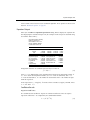
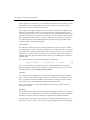
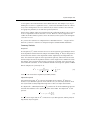
6—Chapter 1. Basic Regression Analysis
Specifying an Equation in EViews
When you create an equation object, a specification dialog box is displayed.
You need to specify three things
in this dialog: the equation specification, the estimation method,
and the sample to be used in
estimation.
In the upper edit box, you can
specify the equation: the dependent (left-hand side) and independent (right-hand side)
variables and the functional
form. There are two basic ways
of specifying an equation: “by
list” and “by formula” or “by
expression”. The list method is
easier but may only be used
with unrestricted linear specifications; the formula method is more general and must be used to specify nonlinear models
or models with parametric restrictions.
Specifying an Equation by List
The simplest way to specify a linear equation is to provide a list of variables that you wish
to use in the equation. First, include the name of the dependent variable or expression, followed by a list of explanatory variables. For example, to specify a linear consumption function, CS regressed on a constant and INC, type the following in the upper field of the
Equation Specification dialog:
cs c inc
Note the presence of the series name C in the list of regressors. This is a built-in EViews
series that is used to specify a constant in a regression. EViews does not automatically
include a constant in a regression so you must explicitly list the constant (or its equivalent)
as a regressor. The internal series C does not appear in your workfile, and you may not use
it outside of specifying an equation. If you need a series of ones, you can generate a new
series, or use the number 1 as an auto-series.
You may have noticed that there is a pre-defined object C in your workfile. This is the
default coefficient vector—when you specify an equation by listing variable names, EViews
stores the estimated coefficients in this vector, in the order of appearance in the list. In the
Specifying an Equation in EViews—7
example above, the constant will be stored in C(1) and the coefficient on INC will be held in
C(2).
Lagged series may be included in statistical operations using the same notation as in generating a new series with a formula—put the lag in parentheses after the name of the series.
For example, the specification:
cs cs(-1) c inc
tells EViews to regress CS on its own lagged value, a constant, and INC. The coefficient for
lagged CS will be placed in C(1), the coefficient for the constant is C(2), and the coefficient
of INC is C(3).
You can include a consecutive range of lagged series by using the word “to” between the
lags. For example:
cs c cs(-1 to -4) inc
regresses CS on a constant, CS(-1), CS(-2), CS(-3), CS(-4), and INC. If you don't include the
first lag, it is taken to be zero. For example:
cs c inc(to -2) inc(-4)
regresses CS on a constant, INC, INC(-1), INC(-2), and INC(-4).
You may include auto-series in the list of variables. If the auto-series expressions contain
spaces, they should be enclosed in parentheses. For example:
log(cs) c log(cs(-1)) ((inc+inc(-1)) / 2)
specifies a regression of the natural logarithm of CS on a constant, its own lagged value, and
a two period moving average of INC.
Typing the list of series may be cumbersome, especially if you are working with many
regressors. If you wish, EViews can create the specification list for you. First, highlight the
dependent variable in the workfile window by single clicking on the entry. Next, CTRL-click
on each of the explanatory variables to highlight them as well. When you are done selecting
all of your variables, double click on any of the highlighted series, and select Open/Equation…, or right click and select Open/as Equation.... The Equation Specification dialog
box should appear with the names entered in the specification field. The constant C is automatically included in this list; you must delete the C if you do not wish to include the constant.
Specifying an Equation by Formula
You will need to specify your equation using a formula when the list method is not general
enough for your specification. Many, but not all, estimation methods allow you to specify
your equation using a formula.
8—Chapter 1. Basic Regression Analysis
An equation formula in EViews is a mathematical expression involving regressors and coefficients. To specify an equation using a formula, simply enter the expression in the dialog in
place of the list of variables. EViews will add an implicit additive disturbance to this equation and will estimate the parameters of the model using least squares.
When you specify an equation by list, EViews converts this into an equivalent equation formula. For example, the list,
log(cs) c log(cs(-1)) log(inc)
is interpreted by EViews as:
log(cs) = c(1) + c(2)*log(cs(-1)) + c(3)*log(inc)
Equations do not have to have a dependent variable followed by an equal sign and then an
expression. The “=” sign can be anywhere in the formula, as in:
log(urate) - c(1)*dmr = c(2)
The residuals for this equation are given by:
e
log urate – c 1 dmr – c 2 .
(1.1)
EViews will minimize the sum-of-squares of these residuals.
If you wish, you can specify an equation as a simple expression, without a dependent variable and an equal sign. If there is no equal sign, EViews assumes that the entire expression
is the disturbance term. For example, if you specify an equation as:
c(1)*x + c(2)*y + 4*z
EViews will find the coefficient values that minimize the sum of squares of the given expression, in this case (C(1)*X+C(2)*Y+4*Z). While EViews will estimate an expression of this
type, since there is no dependent variable, some regression statistics (e.g. R-squared) are
not reported and the equation cannot be used for forecasting. This restriction also holds for
any equation that includes coefficients to the left of the equal sign. For example, if you specify:
x + c(1)*y = c(2)*z
EViews finds the values of C(1) and C(2) that minimize the sum of squares of (X+C(1)*Y–
C(2)*Z). The estimated coefficients will be identical to those from an equation specified
using:
x = -c(1)*y + c(2)*z
but some regression statistics are not reported.
The two most common motivations for specifying your equation by formula are to estimate
restricted and nonlinear models. For example, suppose that you wish to constrain the coeffi-
Estimating an Equation in EViews—9
cients on the lags on the variable X to sum to one. Solving out for the coefficient restriction
leads to the following linear model with parameter restrictions:
y = c(1) + c(2)*x + c(3)*x(-1) + c(4)*x(-2) + (1-c(2)-c(3)-c(4))
*x(-3)
To estimate a nonlinear model, simply enter the nonlinear formula. EViews will automatically detect the nonlinearity and estimate the model using nonlinear least squares. For
details, see “Nonlinear Least Squares” on page 40.
One benefit to specifying an equation by formula is that you can elect to use a different coefficient vector. To create a new coefficient vector, choose Object/New Object… and select
Matrix-Vector-Coef from the main menu, type in a name for the coefficient vector, and click
OK. In the New Matrix dialog box that appears, select Coefficient Vector and specify how
many rows there should be in the vector. The object will be listed in the workfile directory
with the coefficient vector icon (the little b ).
You may then use this coefficient vector in your specification. For example, suppose you
created coefficient vectors A and BETA, each with a single row. Then you can specify your
equation using the new coefficients in place of C:
log(cs) = a(1) + beta(1)*log(cs(-1))
Estimating an Equation in EViews
Estimation Methods
Having specified your equation, you now need to choose an estimation method. Click on the
Method: entry in the dialog and you will see a drop-down menu listing estimation methods.
Standard, single-equation regression is performed using least squares. The other methods are described in subsequent chapters.
Equations estimated by cointegrating regression, GLM or stepwise, or equations including MA terms, may only be specified by list
and may not be specified by expression. All
other types of equations (among others, ordinary least squares and two-stage least squares,
equations with AR terms, GMM, and ARCH equations) may be specified either by list or
expression. Note that equations estimated by quantile regression may be specified by
expression, but can only estimate linear specifications.
Estimation Sample
You should also specify the sample to be used in estimation. EViews will fill out the dialog
with the current workfile sample, but you can change the sample for purposes of estimation
10—Chapter 1. Basic Regression Analysis
by entering your sample string or object in the edit box (see “Samples” on page 91 of User’s
Guide I for details). Changing the estimation sample does not affect the current workfile
sample.
If any of the series used in estimation contain missing data, EViews will temporarily adjust
the estimation sample of observations to exclude those observations (listwise exclusion).
EViews notifies you that it has adjusted the sample by reporting the actual sample used in
the estimation results:
Dependent Variable: Y
Method: Leas t Squares
Date: 08/08/09 Time: 14:44
Sample (adjust ed): 1959M01 1989M12
Included observations: 340 after adjustments
Here we see the top of an equation output view. EViews reports that it has adjusted the
sample. Out of the 372 observations in the period 1959M01–1989M12, EViews uses the 340
observations with valid data for all of the relevant variables.
You should be aware that if you include lagged variables in a regression, the degree of sample adjustment will differ depending on whether data for the pre-sample period are available
or not. For example, suppose you have nonmissing data for the two series M1 and IP over
the period 1959M01–1989M12 and specify the regression as:
m1 c ip ip(-1) ip(-2) ip(-3)
If you set the estimation sample to the period 1959M01–1989M12, EViews adjusts the sample to:
Dependent Variable: M1
Method: Least Squares
Date: 08/08/09 Time: 14:45
Sample: 1960M01 1989M12
Included observations: 360
since data for IP(–3) are not available until 1959M04. However, if you set the estimation
sample to the period 1960M01–1989M12, EViews will not make any adjustment to the sample since all values of IP(-3) are available during the estimation sample.
Some operations, most notably estimation with MA terms and ARCH, do not allow missing
observations in the middle of the sample. When executing these procedures, an error message is displayed and execution is halted if an NA is encountered in the middle of the sample. EViews handles missing data at the very start or the very end of the sample range by
adjusting the sample endpoints and proceeding with the estimation procedure.
Estimation Options
EViews provides a number of estimation options. These options allow you to weight the
estimating equation, to compute heteroskedasticity and auto-correlation robust covariances,
Equation Output—11
and to control various features of your estimation algorithm. These options are discussed in
detail in “Estimation Options” on page 42.
Equation Output
When you click OK in the Equation Specification dialog, EViews displays the equation window displaying the estimation output view (the examples in this chapter are obtained using
the workfile “Basics.WF1”):
Dependent Variable: LOG(M1)
Method: Least Squares
Date: 08/08/09 Time: 14:51
Sample: 1959M01 1989M12
I ncluded observations: 372
Variable
Coefficient
Std. E rror
t-Stat istic
Prob.
C
LOG(IP)
TB3
-1. 699912
1.765866
-0. 011895
0.164954
0.043546
0.004628
-10.30539
40.55199
-2.570016
0.0000
0.0000
0.0106
R-squared
Adjusted R-squared
S.E. of regression
Sum squared resid
Log likelihood
F-st atist ic
Prob(F-stat istic)
0.886416
0.885800
0.187183
12. 92882
97. 00979
1439.848
0.000000
Mean dependent var
S.D. dependent var
Akaike info crit erion
Schwarz criterion
Hannan-Quinn criter.
Durbin-W at son st at
5.663717
0.553903
-0. 505429
-0. 473825
-0. 492878
0.008687
Using matrix notation, the standard regression may be written as:
y
Xb e
(1.2)
where y is a T -dimensional vector containing observations on the dependent variable, X
is a T – k matrix of independent variables, b is a k -vector of coefficients, and e is a
T -vector of disturbances. T is the number of observations and k is the number of righthand side regressors.
In the output above, y is log(M1), X consists of three variables C, log(IP), and TB3, where
T
372 and k
3.
Coefficient Results
Regression Coefficients
The column labeled “Coefficient” depicts the estimated coefficients. The least squares
regression coefficients b are computed by the standard OLS formula:
b
–1
X„X X„y
(1.3)
12—Chapter 1. Basic Regression Analysis
If your equation is specified by list, the coefficients will be labeled in the “Variable” column
with the name of the corresponding regressor; if your equation is specified by formula,
EViews lists the actual coefficients, C(1), C(2), etc.
For the simple linear models considered here, the coefficient measures the marginal contribution of the independent variable to the dependent variable, holding all other variables
fixed. If you have included “C” in your list of regressors, the corresponding coefficient is the
constant or intercept in the regression—it is the base level of the prediction when all of the
other independent variables are zero. The other coefficients are interpreted as the slope of
the relation between the corresponding independent variable and the dependent variable,
assuming all other variables do not change.
Standard Errors
The “Std. Error” column reports the estimated standard errors of the coefficient estimates.
The standard errors measure the statistical reliability of the coefficient estimates—the larger
the standard errors, the more statistical noise in the estimates. If the errors are normally distributed, there are about 2 chances in 3 that the true regression coefficient lies within one
standard error of the reported coefficient, and 95 chances out of 100 that it lies within two
standard errors.
The covariance matrix of the estimated coefficients is computed as:
var b 2
–1
s X„X s
2
eˆ „eˆ † T – k eˆ
y – Xb
(1.4)
where eˆ is the residual. The standard errors of the estimated coefficients are the square
roots of the diagonal elements of the coefficient covariance matrix. You can view the whole
covariance matrix by choosing View/Covariance Matrix.
t-Statistics
The t-statistic, which is computed as the ratio of an estimated coefficient to its standard
error, is used to test the hypothesis that a coefficient is equal to zero. To interpret the t-statistic, you should examine the probability of observing the t-statistic given that the coefficient is equal to zero. This probability computation is described below.
In cases where normality can only hold asymptotically, EViews will report a z-statistic
instead of a t-statistic.
Probability
The last column of the output shows the probability of drawing a t-statistic (or a z-statistic)
as extreme as the one actually observed, under the assumption that the errors are normally
distributed, or that the estimated coefficients are asymptotically normally distributed.
This probability is also known as the p-value or the marginal significance level. Given a pvalue, you can tell at a glance if you reject or accept the hypothesis that the true coefficient
Equation Output—13
is zero against a two-sided alternative that it differs from zero. For example, if you are performing the test at the 5% significance level, a p-value lower than 0.05 is taken as evidence
to reject the null hypothesis of a zero coefficient. If you want to conduct a one-sided test,
the appropriate probability is one-half that reported by EViews.
For the above example output, the hypothesis that the coefficient on TB3 is zero is rejected
at the 5% significance level but not at the 1% level. However, if theory suggests that the
coefficient on TB3 cannot be positive, then a one-sided test will reject the zero null hypothesis at the 1% level.
The p-values for t-statistics are computed from a t-distribution with T – k degrees of freedom. The p-value for z-statistics are computed using the standard normal distribution.
Summary Statistics
R-squared
2
The R-squared ( R ) statistic measures the success of the regression in predicting the values
2
of the dependent variable within the sample. In standard settings, R may be interpreted as
the fraction of the variance of the dependent variable explained by the independent variables. The statistic will equal one if the regression fits perfectly, and zero if it fits no better
than the simple mean of the dependent variable. It can be negative for a number of reasons.
For example, if the regression does not have an intercept or constant, if the regression contains coefficient restrictions, or if the estimation method is two-stage least squares or ARCH.
2
EViews computes the (centered) R as:
R
2
eˆ „eˆ
1 – ------------------------------------- y – y „ y – y T
y
t
Ç yt † T
(1.5)
1
where y is the mean of the dependent (left-hand) variable.
Adjusted R-squared
2
2
One problem with using R as a measure of goodness of fit is that the R will never
2
decrease as you add more regressors. In the extreme case, you can always obtain an R of
one if you include as many independent regressors as there are sample observations.
2
2
2
The adjusted R , commonly denoted as R , penalizes the R for the addition of regressors
2
which do not contribute to the explanatory power of the model. The adjusted R is computed as:
R
2
2 T – 1
1 – 1 – R ------------T–k
2
2
(1.6)
The R is never larger than the R , can decrease as you add regressors, and for poorly fitting models, may be negative.
14—Chapter 1. Basic Regression Analysis
Standard Error of the Regression (S.E. of regression)
The standard error of the regression is a summary measure based on the estimated variance
of the residuals. The standard error of the regression is computed as:
eˆ „eˆ
-----------------T – k s
(1.7)
Sum-of-Squared Residuals
The sum-of-squared residuals can be used in a variety of statistical calculations, and is presented separately for your convenience:
T
eˆ „eˆ
t
Ç yi – Xi „b 2
(1.8)
1
Log Likelihood
EViews reports the value of the log likelihood function (assuming normally distributed
errors) evaluated at the estimated values of the coefficients. Likelihood ratio tests may be
conducted by looking at the difference between the log likelihood values of the restricted
and unrestricted versions of an equation.
The log likelihood is computed as:
l
T
– ---- 1 log 2p log eˆ „eˆ † T 2
(1.9)
When comparing EViews output to that reported from other sources, note that EViews does
not ignore constant terms in the log likelihood.
Durbin-Watson Statistic
The Durbin-Watson statistic measures the serial correlation in the residuals. The statistic is
computed as
T
DW
t
Ç
2
T
2
eˆ t – eˆ t – 1 †
t
Ç eˆ t
2
(1.10)
1
See Johnston and DiNardo (1997, Table D.5) for a table of the significance points of the distribution of the Durbin-Watson statistic.
As a rule of thumb, if the DW is less than 2, there is evidence of positive serial correlation.
The DW statistic in our output is very close to one, indicating the presence of serial correlation in the residuals. See “Serial Correlation Theory,” beginning on page 85, for a more
extensive discussion of the Durbin-Watson statistic and the consequences of serially correlated residuals.
Equation Output—15
There are better tests for serial correlation. In “Testing for Serial Correlation” on page 86,
we discuss the Q-statistic, and the Breusch-Godfrey LM test, both of which provide a more
general testing framework than the Durbin-Watson test.
Mean and Standard Deviation (S.D.) of the Dependent Variable
The mean and standard deviation of y are computed using the standard formulae:
T
y
t
Ç yt † T
T
sy
t
1
Ç yt – y 2
† T – 1 (1.11)
1
Akaike Information Criterion
The Akaike Information Criterion (AIC) is computed as:
AIC
– 2l † T 2k † T
(1.12)
where l is the log likelihood (given by Equation (1.9) on page 14).
The AIC is often used in model selection for non-nested alternatives—smaller values of the
AIC are preferred. For example, you can choose the length of a lag distribution by choosing
the specification with the lowest value of the AIC. See Appendix C. “Information Criteria,”
on page 771, for additional discussion.
Schwarz Criterion
The Schwarz Criterion (SC) is an alternative to the AIC that imposes a larger penalty for
additional coefficients:
– 2l † T k log T † T
SC
(1.13)
Hannan-Quinn Criterion
The Hannan-Quinn Criterion (HQ) employs yet another penalty function:
HQ
– 2 l † T 2k log log T † T
(1.14)
F-Statistic
The F-statistic reported in the regression output is from a test of the hypothesis that all of
the slope coefficients (excluding the constant, or intercept) in a regression are zero. For
ordinary least squares models, the F-statistic is computed as:
F
2
R † k – 1 -------------------------------------------2
1 – R † T – k
(1.15)
Under the null hypothesis with normally distributed errors, this statistic has an F-distribution with k – 1 numerator degrees of freedom and T – k denominator degrees of freedom.