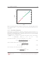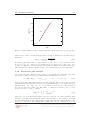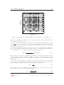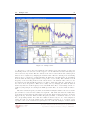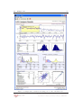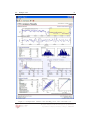
1
Kubios HRV
version 2.0
http://kubios.uku.fi
USER’S GUIDE
October 16, 2008
Mika P. Tarvainen, Ph.D.
([email protected])
and
Juha-Pekka Niskanen, M.Sc.
Biosignal Analysis and Medical Imaging Group (BSAMIG)
(http://bsamig.uku.fi/)
Department of Physics
University of Kuopio
Kuopio, FINLAND
MATLAB. Copyright 1984-2008 The MathWorks, Inc.
MATLAB is a registered trademark of The MathWorks, Inc.
Contents
1 Overview
1.1 System requirements .
1.1.1 Windows . . .
1.1.2 Linux . . . . .
1.2 Installation . . . . . .
1.2.1 Windows . . .
1.2.2 Linux . . . . .
1.3 Uninstallation . . . . .
1.3.1 Windows . . .
1.3.2 Linux . . . . .
1.4 Software home page .
1.5 Structure of this guide
.
.
.
.
.
.
.
.
.
.
.
.
.
.
.
.
.
.
.
.
.
.
.
.
.
.
.
.
.
.
.
.
.
.
.
.
.
.
.
.
.
.
.
.
.
.
.
.
.
.
.
.
.
.
.
.
.
.
.
.
.
.
.
.
.
.
.
.
.
.
.
.
.
.
.
.
.
.
.
.
.
.
.
.
.
.
.
.
.
.
.
.
.
.
.
.
.
.
.
.
.
.
.
.
.
.
.
.
.
.
.
.
.
.
.
.
.
.
.
.
.
.
.
.
.
.
.
.
.
.
.
.
.
.
.
.
.
.
.
.
.
.
.
.
.
.
.
.
.
.
.
.
.
.
.
.
.
.
.
.
.
.
.
.
.
4
5
5
5
5
5
5
6
6
7
7
7
2 Heart rate variability
2.1 Heart beat period and QRS detection . . . . . . . .
2.2 Derivation of HRV time series . . . . . . . . . . . . .
2.3 Preprocessing of HRV time series . . . . . . . . . . .
2.3.1 Smoothness priors based detrending approach
.
.
.
.
.
.
.
.
.
.
.
.
.
.
.
.
.
.
.
.
.
.
.
.
.
.
.
.
.
.
.
.
.
.
.
.
.
.
.
.
.
.
.
.
.
.
.
.
.
.
.
.
.
.
.
.
9
10
11
13
13
3 Analysis methods
3.1 Time-domain methods . . . . . . . . .
3.2 Frequency-domain methods . . . . . .
3.3 Nonlinear methods . . . . . . . . . . .
3.3.1 Poincar´e plot . . . . . . . . . .
3.3.2 Approximate entropy . . . . .
3.3.3 Sample entropy . . . . . . . . .
3.3.4 Detrended fluctuation analysis
3.3.5 Correlation dimension . . . . .
3.3.6 Recurrence plot analysis . . . .
3.4 Summary of HRV parameters . . . . .
.
.
.
.
.
.
.
.
.
.
.
.
.
.
.
.
.
.
.
.
.
.
.
.
.
.
.
.
.
.
.
.
.
.
.
.
.
.
.
.
.
.
.
.
.
.
.
.
.
.
.
.
.
.
.
.
.
.
.
.
.
.
.
.
.
.
.
.
.
.
.
.
.
.
.
.
.
.
.
.
.
.
.
.
.
.
.
.
.
.
.
.
.
.
.
.
.
.
.
.
.
.
.
.
.
.
.
.
.
.
.
.
.
.
.
.
.
.
.
.
.
.
.
.
.
.
.
.
.
.
.
.
.
.
.
.
.
.
.
.
.
.
.
.
.
.
.
.
.
.
.
.
.
.
.
.
.
.
.
.
.
.
.
.
.
.
.
.
.
.
.
.
.
.
.
.
.
.
.
.
.
.
.
.
.
.
.
.
.
.
.
.
.
.
.
.
.
.
.
.
.
.
.
.
.
.
.
.
.
.
.
.
.
.
.
.
.
.
.
.
15
15
16
16
17
18
18
19
20
21
23
4 Software description
4.1 Input data formats . . . . . . . .
4.2 The user interface . . . . . . . .
4.2.1 RR interval series options
4.2.2 Data browser . . . . . . .
4.2.3 Analysis options . . . . .
4.2.4 Results view . . . . . . .
.
.
.
.
.
.
.
.
.
.
.
.
.
.
.
.
.
.
.
.
.
.
.
.
.
.
.
.
.
.
.
.
.
.
.
.
.
.
.
.
.
.
.
.
.
.
.
.
.
.
.
.
.
.
.
.
.
.
.
.
.
.
.
.
.
.
.
.
.
.
.
.
.
.
.
.
.
.
.
.
.
.
.
.
.
.
.
.
.
.
.
.
.
.
.
.
.
.
.
.
.
.
.
.
.
.
.
.
.
.
.
.
.
.
.
.
.
.
.
.
.
.
.
.
.
.
.
.
.
.
.
.
25
25
25
25
27
29
30
.
.
.
.
.
.
.
.
.
.
.
.
.
.
.
.
.
.
.
.
.
.
.
.
.
.
.
.
.
.
.
.
.
.
.
.
.
.
.
.
.
.
.
.
.
.
.
.
.
.
.
.
.
.
.
.
.
.
.
.
.
.
.
.
.
.
.
.
.
.
.
.
.
.
.
.
.
.
.
.
.
.
.
.
.
.
.
.
.
.
.
.
.
.
.
.
.
.
.
.
2
.
.
.
.
.
.
.
.
.
.
.
.
.
.
.
.
.
.
.
.
.
.
.
.
.
.
.
.
.
.
.
.
.
.
.
.
.
.
.
.
.
.
.
.
.
.
.
.
.
.
.
.
.
.
.
.
.
.
.
.
.
.
.
.
.
.
.
.
.
.
.
.
.
.
.
.
.
.
.
.
.
.
.
.
.
.
.
.
.
.
.
.
.
.
4.3
4.4
4.2.5 Menus and toolbar buttons
Saving the results . . . . . . . . . .
4.3.1 ASCII-file . . . . . . . . . .
4.3.2 Report sheet . . . . . . . .
4.3.3 MATLABr MAT-file . . .
Setting up the preferences . . . . .
.
.
.
.
.
.
.
.
.
.
.
.
.
.
.
.
.
.
.
.
.
.
.
.
.
.
.
.
.
.
.
.
.
.
.
.
.
.
.
.
.
.
.
.
.
.
.
.
.
.
.
.
.
.
.
.
.
.
.
.
.
.
.
.
.
.
.
.
.
.
.
.
.
.
.
.
.
.
.
.
.
.
.
.
.
.
.
.
.
.
.
.
.
.
.
.
.
.
.
.
.
.
.
.
.
.
.
.
.
.
.
.
.
.
.
.
.
.
.
.
.
.
.
.
.
.
.
.
.
.
.
.
.
.
.
.
.
.
.
.
.
.
.
.
31
33
33
33
35
36
5 Sample runs
40
5.1 Sample run . . . . . . . . . . . . . . . . . . . . . . . . . . . . . . . . . . . . . 40
A Frequently asked questions
46
B Troubleshooting
48
B.1 Windows specific . . . . . . . . . . . . . . . . . . . . . . . . . . . . . . . . . . 48
B.2 Linux specific . . . . . . . . . . . . . . . . . . . . . . . . . . . . . . . . . . . . 49
References
49
3
Chapter 1
Overview
Kubios HRV is an advanced tool for studying the variability of heart beat intervals. Due
to its wide variety of different analysis options and the easy to use interface, the software
is suitable for researchers and clinicians with varying premises. The software is mainly
designed for the analysis of normal human HRV, but should also be usable, e.g., for animal
research.
Kubios HRV includes all the commonly used time- and frequency-domain variables of
HRV. The frequency-domain variables are calculated for both nonparametric (Fourier transform based) and parametric (autoregressive modeling based) spectrum estimates. In addition, several nonlinear HRV variables are calculated such as Poincar´e plot, recurrence plot
analysis, detrended fluctuation analysis, approximate and sample entropies, and correlation
dimension.
The Kubios HRV, heart rate variability (HRV) analysis software1 , is developed by the
Biosignal Analysis and Medical Imaging Group (BSAMIG) at the Department of Physics,
University of Kuopio, Kuopio, Finland. The software is a considerable upgrade to the
previous version (version 1.1) of the software described in [32]. Changes from the previous
version include significantly improved usability, support for new data formats and many
new or updated features. Kubios HRV has been developed using MATLABr Release 2008a
(The MathWorks, Inc.) and was compiled to a deployable standalone application with the
MATLABr Compiler 4.8. The MATLABr Compiler Runtime (MCR) version 7.8 is required
for running Kubios HRV and is included in the Kubios HRV installers.
1 Kuopio University has only limited rights to the software. These limited rights are governed by a certain
license agreement between Kuopio University and The MathWorks, Inc.
4
5
1.1. System requirements
1.1
System requirements
The system requirements given below should be considered as recommended system requirements. The software may work also with lower system specifications, but will probably
function slower or with reduced usability.
1.1.1
Windows
• Operating system: Microsoftr Windows 2000, XP or Vista
• Processor: Intelr Pentium 4 and above (or equivalent 32-bit (x86) processor)
• Memory: 512 MB of RAM (1024 MB or higher recommended)
• Disk space: about 500 MB
• Desktop resolution of 1024×768 or higher
• The MATLABr Compiler Runtime 7.8 (included in the Kubios HRV installer)
1.1.2
Linux
• Operating system: a Linux distribution with kernel 2.4.x or 2.6.x and glibc (glibc6)
2.3.4 and above.
• Processor: Intelr Pentium 4 and above (or equivalent 32-bit (x86) processor)
• Memory: 512 MB of RAM (1024 MB or higher recommended)
• Desktop resolution of 1024×768 or higher
• Disk space: about 460 MB
• The MATLABr Compiler Runtime 7.8 (included in the Kubios HRV installer)
1.2
1.2.1
Installation
Windows
Make sure that you have administrator privileges and run the Kubios HRV installer file.
Follow the instructions given in the setup wizard to complete installation. You can launch
the Kubios HRV by selecting it from the created Start Menu folder or by clicking the Desktop
icon (if created). Please note that the starting of Kubios HRV also starts the MATLABr
Compiler Runtime and may take some time especially with older computers.
1.2.2
Linux
Run the Kubios HRV installer by typing sh KubiosHRV-linux-2.0 x86.run in the terminal and follow the instructions given on screen. The Kubios HRV installer also includes
the MATLABr Compiler Runtime. NOTE: If you run the installer as root, Kubios
HRV will be installed on your computer system wide for all users. If you want
to install Kubios HRV only for yourself, run the installer as local user.
Kubios HRV
version 2.0
Biosignal Analysis and Medical Imaging Group (BSAMIG)
Department of Physics, University of Kuopio, FINLAND
6
1.3. Uninstallation
1.3
Uninstallation
The Kubios HRV can be uninstalled either automatically using the uninstaller or manually
if the uninstaller fails for some reason. Both methods for uninstallation are described in the
following.
1.3.1
Windows
Automated uninstall
The preferred and the most straightforward way of uninstalling Kubios HRV is
to use the automated uninstaller.
The uninstaller can be launched by selecting
“Uninstall Kubios HRV” from the software’s Start menu folder (the default Start
menu folder is Kubios HRV). The software can also be uninstalled from the “Add
or Remove Programs” under the Windows Control Panel.
The uninstaller does
not remove your preferences settings.
These have to be deleted manually from
C:\Documents and Settings\<username>\Application Data\KubiosHRV.
Manual uninstall
The manual uninstallation should be conducted only if the automated uninstallation fails.
The Kubios HRV can be completely uninstalled manually by deleting the following files,
folders, and registry entries:
• Delete the install folder (by default C:\Program Files\Kubios HRV) and all the subfolders and files in it.
• Delete the KubiosHRV folder (if exists) from
(Windows XP/2000:)
C:\Documents and Settings\<username>\Application Data\
(Windows Vista:)
C:\Users\<username>\AppData\Roaming\
• Delete the Kubios HRV quick launch icons (if exist) from
(Windows XP/2000:)
C:\Documents and Settings\<username>\Application Data\Microsoft\
Internet Explorer\Quick Launch\
(Windows Vista:)
C:\Users\<username>\AppData\Roaming\Microsoft\
Internet Explorer\Quick Launch\
• Delete desktop icons (if exist) from
(Windows XP/2000:)
C:\Documents and Settings\All Users\Desktop\
(Windows Vista:)
C:\Users\Public\Desktop\
• Delete the possible Start menu entries from
(Windows XP/2000:)
C:\Documents and Settings\All Users\Start Menu\Programs\
(Windows Vista:)
C:\ProgramData\Microsoft\Windows\Start Menu\Programs\
Kubios HRV
version 2.0
Biosignal Analysis and Medical Imaging Group (BSAMIG)
Department of Physics, University of Kuopio, FINLAND
7
1.4. Software home page
• Remove the MATLAB Compiler Runtime entry
(<KubiosHRV install dir>\MCR\v78\runtime\win32) from the system path
• Manual removal of the Kubios HRV Analysis entry from the Windows’ “Add or Remove Programs” list requires modifying registry. A thorough instructions on how to
manually remove programs from the “Add or Remove Programs” list is available on
the Microsoft support web site at http://support.microsoft.com/?kbid=314481.
1.3.2
Linux
Automated uninstall
Open terminal and change directory to the Kubios HRV install directory. Run the command
sh uninstall_kubios.sh and follow instructions given on screen. NOTE: You may need
root privileges for running the uninstaller if you have installed Kubios HRV as root.
Manual uninstall
Open a terminal and run the following commands.
In the commands replace
<Kubios HRV install dir> with the Kubios HRV install directory. NOTE: You may need
root privileges for running these commands if you have installed Kubios HRV as root.
• Uninstall Kubios HRV menu entries
xdg-desktop-menu uninstall <Kubios HRV install dir>/BSAMIG-KubiosHRV.desktop
• Uninstall Kubios HRV desktop icons
xdg-desktop-icon uninstall <Kubios HRV install dir>/BSAMIG-KubiosHRV.desktop
• Delete the Kubios HRV install directory
rm -rf <Kubios HRV install dir>
1.4
Software home page
The Kubios HRV (version 2.0) home page on the web can be found at
http://kubios.uku.fi/
where you can find current information on the software and download possible updates
and related material.
1.5
Structure of this guide
The aim of this guidebook is to help the user to get started with Kubios HRV. It should
not, however, be thought of as being an easy to follow step by step manual, but more like
a reference material from which you can probably find answers to your problems related to
HRV analysis or usability of the software. The structure of this guide is as follows.
After the overview chapter, from where you will find useful information about the system
requirements and installation, an introduction to heart rate variability is given in Chapter 2.
This chapter starts with a short discussion on the control systems of heart rate after which
the extraction of heart beat periods is discussed and the derivation of HRV time series is
Kubios HRV
version 2.0
Biosignal Analysis and Medical Imaging Group (BSAMIG)
Department of Physics, University of Kuopio, FINLAND
8
1.5. Structure of this guide
described. The rest of the chapter is focused on the preprocessing of HRV data and gives a
detailed description of the smoothness priors based detrending approach.
In Chapter 3, the analysis methods included in the software are described. The descriptions of the methods are divided into time-domain, frequency-domain, nonlinear, and
time-varying categories and a summary of the methods is given at the end of the chapter.
For most of the methods, exact formulas for the different variables are given and possible
parameter selections are pointed out.
In Chapter 4, the description of the features and usage of the software is given. First,
the input data formats supported by the software are described and then the user interface
through which the software is operated is described. Then, different options for saving the
analysis results are described and, finally, instructions on how to set up the preference values
for the analysis options are given.
In Chapter 5, two sample runs of the software are presented. The first sample run
describes how to analyze the lying and standing periods of the orthostatic test measurement
(distributed along this software) separately as stationary segments. The second sample run,
on the other hand, describes the time-varying analysis procedure of the same measurement.
In Appendix A, some frequently asked questions with answers are given. The questions
are selected based on the feedback obtained from the users of the previous version of this
software.
Finally, in Appendix B, workarounds for some commonly encountered technical problems
are given.
Kubios HRV
version 2.0
Biosignal Analysis and Medical Imaging Group (BSAMIG)
Department of Physics, University of Kuopio, FINLAND
Chapter 2
Heart rate variability
Heart rate variability (HRV) describes the variations between consecutive heartbeats. The
rhythm of the heart is controlled by the sinoatrial (SA) node, which is modulated by both
the sympathetic and parasympathetic branches of the autonomic nervous system. Sympathetic activity tends to increase heart rate (HR↑) and its response is slow (few seconds)
[3]. Parasympathetic activity, on the other hand, tends to decrease heart rate (HR↓) and
mediates faster (0.2–0.6 seconds) [3]. In addition to central control, there are some feedback
mechanisms that can provide quick reflexes. One such mechanism is the arterial baroreflex.
This reflex is based on baroreceptors which are located on the walls of some large vessels
and can sense the stretching of vessel walls caused by pressure increase. Both sympathetic
and parasympathetic activity are influenced by baroreceptor stimulation trough a specific
baroreflex arc, Fig. 2.1.
The continuous modulation of the sympathetic and parasympathetic innervations results
in variations in heart rate. The most conspicuous periodic component of HRV is the socalled respiratory sinus arrhythmia (RSA) which is considered to range from 0.15 to 0.4
Hz [3]. In addition to the physiological influence of breathing on HRV, this high frequency
(HF) component is generally believed to be of parasympathetic origin. Another widely
studied component of HRV is the low frequency (LF) component usually ranging from 0.04
to 0.15 Hz including the component referred to as the 10-second rhythm or the Mayer wave
[3]. The rhythms within the LF band have been thought to be of both sympathetic and
parasympathetic origin [3] even though some researchers have suggested them to be mainly
of sympathetic origin [25]. The fluctuations below 0.04 Hz, on the other hand, have not
been studied as much as the higher frequencies. These frequencies are commonly divided
into very low frequency (VLF, 0.003-0.04 Hz) and ultra low frequency (ULF, 0-0.003 Hz)
bands, but in case of short-term recordings the ULF band is generally omitted [45]. These
lowest frequency rhythms are characteristic for HRV signals and have been related to, e.g.,
humoral factors such as the thermoregulatory processes and renin-angiotensin system [3].
Even though HRV has been studied extensively during the last decades within which
numerous research articles have been published, the practical use of HRV have reached
general consensus only in two clinical applications [45]. That is, it can be used as a predictor
of risk after myocardial infarction [24, 19] and as an early warning sign of diabetic neuropathy
[5, 33]. In addition, HRV has been found to correlate with, e.g., age, mental and physical
stress, and attention, see, e.g., the review in [3].
The term HRV refers, in general, to changes in heart beat interval which is a reciprocal
of the heart rate. This is also the case here. The starting point for HRV analysis is the ECG
recording from which the HRV time series can be extracted. In the formulation of the HRV
9
10
2.1. Heart beat period and QRS detection
Vasomotor
sympathetic
Sympathetic
∆Vv
Sympathetic
VC
Sympathetic
HR
Vagal
HR
TPR
HEART
Left ven- Vs
tricle
×
CO
×
BPa
+
Baroreceptors
Figure 2.1: The four baroreflex pathways (redrawn from [41]). Variation in venous volume
(∆Vv ), left ventricular contractility (VC), sympathetic and parasympathetic (vagal) control
of heart rate (HR), stroke volume (Vs ), cardiac output (CO), total peripheral resistance
(TPR), and arterial blood pressure (BPa ).
time series, a fundamental issue is the determination of heart beat period.
2.1
Heart beat period and QRS detection
The aim in HRV analysis is to examine the sinus rhythm modulated by the autonomic nervous system. Therefore, one should technically detect the occurrence times of the SA-node
action potentials. This is, however, practically impossible and, thus, the fiducial points for
the heart beat is usually determined from the ECG recording. The nearest observable activity in the ECG compared to SA-node firing is the P-wave resulting from atrial depolarization
(see Fig. 2.2) and, thus, the heart beat period is generally defined as the time difference
between two successive P-waves. The signal-to-noise ratio of the P-wave is, however, clearly
lower than that of the strong QRS complex which results primarily from ventricular depolarization. Therefore, the heart beat period is commonly evaluated as the time difference
between the easily detectable QRS complexes.
A typical QRS detector consists of a preprocessing part followed by a decision rule.
Several different QRS detectors have been proposed within last decades [46, 34, 35, 17, 12].
For an easy to read review of these methods, see [1]. The preprocessing of the ECG usually
includes at least bandpass filtering to reduce power line noise, baseline wander, muscle noise,
and other interference components. The passband can be set to approximately 5–30 Hz
which covers most of the frequency content of QRS complex [34]. In addition, preprocessing
can include differentiation and/or squaring of the samples. After preprocessing, the decision
rules are applied to determine whether or not a QRS complex has occurred. The decision
rule usually includes an amplitude threshold which is adjusted adaptively as the detection
progresses. In addition, the average heart beat period is often used in the decision. The
fiducial point is generally selected to be the R-wave and the corresponding time instants are
given as the output of the detector.
The accuracy of the R-wave occurrence time estimates is often required to be 1–2 ms
and, thus, the sampling frequency of the ECG should be at least 500–1000 Hz [45]. If the
Kubios HRV
version 2.0
Biosignal Analysis and Medical Imaging Group (BSAMIG)
Department of Physics, University of Kuopio, FINLAND
2.2. Derivation of HRV time series
11
Figure 2.2: Electrophysiology of the heart (redrawn from [26]). The different waveforms for
each of the specialized cells found in the heart are shown. The latency shown approximates
that normally found in the healthy heart.
sampling frequency of the ECG is less than 500 Hz, the errors in R-wave occurrence times
can cause critical distortion to HRV analysis results, especially to spectrum estimates [30].
The distortion of the spectrum is even bigger if the overall variability in heart rate is small
[38]. The estimation accuracy can however be improved by interpolating the QRS complex
e.g. by using a cubic spline interpolation [9] or some model based approach [4]. It should
be, however, noted that when the SA-node impulses are of interest there is an unavoidable
estimation error of approximately 3 ms due to fluctuations in the AV-nodal conduction time
[41].
2.2
Derivation of HRV time series
After the QRS complex occurrence times have been estimated, the HRV time series can be
derived. The inter-beat intervals or RR intervals are obtained as differences between successive R-wave occurrence times. That is, the n’th RR interval is obtained as the difference
between the R-wave occurrence times RRn = tn − tn−1 . In some context, normal-to-normal
(NN) may also be used when referring to these intervals indicating strictly intervals between
successive QRS complexes resulting from SA-node depolarization [45]. In practice, the NN
and RR intervals appear to be the same and, thus, the term RR is preferred here.
The time series constructed from all available RR intervals is, clearly, not equidistantly
sampled, but has to be presented as a function of time, i.e. as values (tn ,RRn ). This fact
has to be taken into account before frequency-domain analysis. In general, three different
approaches have been used to get around this issue [45]. The simplest approach that have
been adopted in, e.g., [2] is to assume equidistant sampling and calculate the spectrum
directly from the RR interval tachogram (RR intervals as a function of beat number), see
Kubios HRV
version 2.0
Biosignal Analysis and Medical Imaging Group (BSAMIG)
Department of Physics, University of Kuopio, FINLAND
12
2.2. Derivation of HRV time series
Derived RR intervals
RR1
RR2
t0
RR3
t1
RR4
t2
t3
RR5
t4
t5
RR interval tachogram
RR2
RR
RR
3
5
RR
RR
4
1
1
2
3
4
5
RR interval series (with two possible ways of interpolation)
RR2
RR3
RR4
RR1
t
1
RR5
t
2
t
3
t
4
t
5
Figure 2.3: Derivation of two HRV signals from ECG: the interval tachogram (middle panel)
and interpolated RR interval series (bottom panel).
the left panel of Fig. 2.3. This assumption can, however, cause distortion into the spectrum
[28]. This distortion becomes substantial when the variability is large in comparison with the
mean level. Furthermore, the spectrum can not be considered to be a function of frequency
but rather of cycles per beat [10]. Another common approach, adopted in this software,
is to use interpolation methods for converting the non-equidistantly sampled RR interval
time series (also called the interval function) to equidistantly sampled [45], see the right
panel of Fig. 2.3. One choice for the interpolation method is the cubic spline interpolation
[28]. After interpolation, regular spectrum estimation methods can be applied. The third
general approach called the spectrum of counts considers a series of impulses (delta functions
positioned at beat occurrence times) [11]. This approach relies on the generally accepted
integral pulse frequency modulator (IPFM) which aims to model the neural modulation of
the SA-node [41]. According to this model, the modulating signal is integrated until a
reference level is achieved after which an impulse is emitted and the integrator is set to zero.
The spectrum of the series of events can be calculated, e.g., by first lowpass filtering the
event series and then calculating the spectrum of the resulting signal [10].
Kubios HRV
version 2.0
Biosignal Analysis and Medical Imaging Group (BSAMIG)
Department of Physics, University of Kuopio, FINLAND
2.3. Preprocessing of HRV time series
2.3
13
Preprocessing of HRV time series
Any artifact in the RR interval time series may interfere the analysis of these signals. The
artifacts within HRV signals can be divided into technical and physiological artifacts. The
technical artifacts can include missing or additional QRS complex detections and errors
in R-wave occurrence times. These artifacts may be due to measurement artifacts or the
computational algorithm. The physiological artifacts, on the other hand, include ectopic
beats and arrhythmic events. In order to avoid the interference of such artifacts, the ECG
recording and the corresponding event series should always be manually checked for artifacts
and only artifact-free sections should be included in the analysis [45]. Alternatively, if the
amount of artifact-free data is insufficient, proper interpolation methods can be used to
reduce these artifacts, see, e.g., [21, 22, 29].
Another common feature that can alter the analysis significantly are the slow linear
or more complex trends within the analyzed time series. Such slow nonstationarities are
characteristic for HRV signals and should be considered before the analysis. The origins of
nonstationarities in HRV are discussed, e.g., in [3]. Two kinds of methods have been used
to get around the nonstationarity problem. In [49], it was suggested that HRV data should
be systematically tested for nonstationarities and that only stationary segments should be
analyzed. Representativeness of these segments in comparison with the whole HRV signal
was, however, questioned in [15]. Other methods try to remove the slow nonstationary trends
from the HRV signal before analysis. The detrending is usually based on first order [23, 31]
or higher order polynomial [39, 31] models. In addition, this software includes an advanced
detrending procedure originally presented in [44]. This approach is based on smoothness
priors regularization.
2.3.1
Smoothness priors based detrending approach
Let z ∈ RN denote the RR interval time series which can be considered to consist of two
components
z = zstat + ztrend
(2.1)
where zstat is the nearly stationary RR interval series of interest, ztrend is the low frequency
aperiodic trend component, and N is the number of RR intervals. Suppose that the trend
component can be modeled with a linear observation model as
ztrend = Hθ + e
(2.2)
where H ∈ RN ×p is the observation matrix, θ ∈ Rp are the regression parameters, and e is
the observation error. The task is then to estimate the parameters by some fitting procedure
so that zˆtrend = H θˆ can be used as the estimate of the trend. The properties of the estimate
depend strongly on the properties of the basis vectors (columns of the matrix H) in the
fitting. A widely used method for the solution of the estimate θˆ is the least squares method.
However, a more general approach for the estimation of θˆ is used here. That is, the so-called
regularized least squares solution
θˆλ = arg min kz − Hθk2 + λ2 kDd (Hθ)k2
(2.3)
θ
where λ is the regularization parameter and Dd indicates the discrete approximation of the
d’th derivative operator. This is clearly a modification of the ordinary least squares solution
to the direction in which the side norm kDd (Hθ)k gets smaller. In this way, prior information
Kubios HRV
version 2.0
Biosignal Analysis and Medical Imaging Group (BSAMIG)
Department of Physics, University of Kuopio, FINLAND
14
1
1
Magnitude
Magnitude
2.3. Preprocessing of HRV time series
0.5
0
0.5
Re
la
20
tive 0.25
freq
uen
cy
0
0
10
e
te tim
iscre
0.5
0
0
D
(a)
0.1
0.2
0.3
0.4
Relative frequency
(b)
0.5
Figure 2.4: a) Time-varying frequency response of L (N − 1 = 50 and λ = 10). Only the first
half of the frequency response is presented, since the other half is identical. b) Frequency
responses, obtained from the middle row of L (cf. bold lines), for λ = 1, 2, 4, 10, 20, 100,
and 500. The corresponding cut-off frequencies are 0.213, 0.145, 0.101, 0.063, 0.045, 0.021
and 0.010 times the sampling frequency.
about the predicted trend Hθ can be implemented to the estimation. The solution of (2.3)
can be written in the form
θˆλ = (H T H + λ2 H T DdT Dd H)−1 H T z
(2.4)
and the estimate for the trend which is to be removed as
zˆtrend = H θˆλ .
(2.5)
The selection of the observation matrix H can be implemented according to some known
properties of the data z. For example, a generic set of Gaussian shaped functions or sigmoids
can be used. Here, however, the trivial choice of identity matrix H = I ∈ RN ×N is used. In
this case, the regularization part of (2.3) can be understood to draw the solution towards
the null space of the regularization matrix Dd . The null space of the second order difference
matrix contains all first order curves and, thus, D2 is a good choice for estimating the
aperiodic trend of RR series. With these specific choices, the detrended nearly stationary
RR series can be written as
zˆstat = z − H θˆλ = (I − (I + λ2 D2T D2 )−1 )z.
(2.6)
In order to demonstrate the properties of the proposed detrending method, its frequency
response is considered. Equation (2.5) can be written as zˆstat = Lz, where L = I −
(I + λ2 D2T D2 )−1 corresponds to a time-varying finite impulse response highpass filter. The
frequency response of L for each discrete time point, obtained as a Fourier transform of its
rows, is presented in Fig. 2.4 (a). It can be seen that the filter is mostly constant but the
beginning and end of the signal are handled differently. The filtering effect is attenuated for
the first and last elements of z and, thus, the distortion of end points of data is avoided.
The effect of the smoothing parameter λ on the frequency response of the filter is presented
in Fig. 2.4 (b). The cutoff frequency of the filter decreases when λ is increased. Besides the
λ parameter the frequency response naturally depends on the sampling rate of signal z.
Kubios HRV
version 2.0
Biosignal Analysis and Medical Imaging Group (BSAMIG)
Department of Physics, University of Kuopio, FINLAND
Chapter 3
Analysis methods
In this chapter, the analysis methods used in the software are introduced. The presented
methods are mainly based on the guidelines given in [45]. The presentation of the methods
is divided into three categories, i.e. time-domain, frequency-domain and nonlinear methods.
The methods summarized in Table 3.1.
3.1
Time-domain methods
The time-domain methods are the simplest to perform since they are applied straight to
the series of successive RR interval values. The most evident such measure is the mean
value of RR intervals (RR) or, correspondingly, the mean HR (HR). In addition, several
variables that measure the variability within the RR series exist. The standard deviation of
RR intervals (SDNN) is defined as
v
u
N
u 1 X
(3.1)
(RRj − RR)2
SDNN = t
N − 1 j=1
where RRj denotes the value of j’th RR interval and N is the total number of successive
intervals. The SDNN reflects the overall (both short-term and long-term) variation within
the RR interval series, whereas the standard deviation of successive RR interval differences
(SDSD) given by
q
SDSD =
E{∆RR2j } − E{∆RRj }2
(3.2)
can be used as a measure of the short-term variability. For stationary RR series E{∆RRj } =
E{RRj+1 } − E{RRj } = 0 and SDSD equals the root mean square of successive differences
(RMSSD) given by
v
u
−1
X
u 1 N
(RRj+1 − RRj )2 .
(3.3)
RMSSD = t
N − 1 j=1
Another measure calculated from successive RR interval differences is the NN50 which is
the number of successive intervals differing more than 50 ms or the corresponding relative
amount
NN50
pNN50 =
× 100%.
(3.4)
N −1
15
16
3.2. Frequency-domain methods
In addition to the above statistical measures, there are some geometric measures that
are calculated from the RR interval histogram. The HRV triangular index is obtained as
the integral of the histogram (i.e. total number of RR intervals) divided by the height of the
histogram which depends on the selected bin width. In order to obtain comparable results,
a bin width of 1/128 seconds is recommended [45]. Another geometric measure is the TINN
which is the baseline width of the RR histogram evaluated through triangular interpolation,
see [45] for details.
3.2
Frequency-domain methods
In the frequency-domain methods, a power spectrum density (PSD) estimate is calculated for
the RR interval series. The regular PSD estimators implicitly assume equidistant sampling
and, thus, the RR interval series is converted to equidistantly sampled series by interpolation
methods prior to PSD estimation. In the software a cubic spline interpolation method is
used. In HRV analysis, the PSD estimation is generally carried out using either FFT based
methods or parametric AR modeling based methods. For details on these methods see, e.g.,
[27]. The advantage of FFT based methods is the simplicity of implementation, while the AR
spectrum yields improved resolution especially for short samples. Another property of AR
spectrum that has made it popular in HRV analysis is that it can be factorized into separate
spectral components. The disadvantages of the AR spectrum are the complexity of model
order selection and the contingency of negative components in the spectral factorization.
Nevertheless, it may be advantageous to calculate the spectrum with both methods to have
comparable results.
In this software, the HRV spectrum is calculated with FFT based Welch’s periodogram
method and with the AR method. Spectrum factorization in AR method is optional. In
the Welch’s periodogram method the HRV sample is divided into overlapping segments.
The spectrum is then obtained by averaging the spectra of these segments. This method
decreases the variance of the FFT spectrum.
The generalized frequency bands in case of short-term HRV recordings are the very low
frequency (VLF, 0–0.04 Hz), low frequency (LF, 0.04–0.15 Hz), and high frequency (HF,
0.15–0.4 Hz). The frequency-domain measures extracted from the PSD estimate for each
frequency band include absolute and relative powers of VLF, LF, and HF bands, LF and
HF band powers in normalized units, the LF/HF power ratio, and peak frequencies for each
band (see Table 3.1). In the case of FFT spectrum, absolute power values for each frequency
band are obtained by simply integrating the spectrum over the band limits. In the case of
AR spectrum, on the other hand, if factorization is enabled distinct spectral components
emerge for each frequency band with a proper selection of the model order and the absolute
power values are obtained directly as the powers of these components. If factorization is
disabled the AR spectrum powers are calculated as for the FFT spectrum. The band powers
in relative and normalized units are obtained from the absolute values as described in Table
3.1.
3.3
Nonlinear methods
Considering the complex control systems of the heart it is reasonable to assume that nonlinear mechanisms are involved in the genesis of HRV. The nonlinear properties of HRV
have been analyzed using measures such as Poincar´e plot [6, 7], approximate and sample
entropy [40, 13], detrended fluctuation analysis [36, 37], correlation dimension [16, 18], and
Kubios HRV
version 2.0
Biosignal Analysis and Medical Imaging Group (BSAMIG)
Department of Physics, University of Kuopio, FINLAND
17
3.3. Nonlinear methods
x
1000
x
950
2
1
850
SD1
RR
j+1
(ms)
900
SD2
800
750
700
650
650
700
750
800 850
RR (ms)
j
900
950 1000
Figure 3.1: Poincar´e plot analysis with the ellipse fitting procedure. SD1 and SD2 are the
standard deviations in the directions x1 and x2 , where x2 is the line-of-identity for which
RRj = RRj+1 .
recurrence plots [48, 47, 50]. During the last years, the number of studies utilizing such
methods have increased substantially. The downside of these methods is still, however, the
difficulty of physiological interpretation of the results.
3.3.1
Poincar´
e plot
One commonly used nonlinear method that is simple to interpret is the so-called Poincar´e
plot. It is a graphical representation of the correlation between successive RR intervals,
i.e. plot of RRj+1 as a function of RRj as described in Fig. 3.1. The shape of the plot
is the essential feature. A common approach to parameterize the shape is to fit an ellipse
to the plot as shown in Fig. 3.1. The ellipse is oriented according to the line-of-identity
(RRj = RRj+1 ) [6]. The standard deviation of the points perpendicular to the line-ofidentity denoted by SD1 describes short-term variability which is mainly caused by RSA. It
can be shown that SD1 is related to the time-domain measure SDSD according to [6]
SD12 =
1
SDSD2 .
2
(3.5)
The standard deviation along the line-of-identity denoted by SD2, on the other hand, describes long-term variability and has been shown to be related to time-domain measures
SDNN and SDSD by [6]
1
SD22 = 2 SDNN2 − SDSD2 .
(3.6)
2
The standard Poincar´e plot can be considered to be of the first order. The second order plot
would be a three dimensional plot of values (RRj , RRj+1 , RRj+2 ). In addition, the lag can
be bigger than 1, e.g., the plot (RRj , RRj+2 ).
Kubios HRV
version 2.0
Biosignal Analysis and Medical Imaging Group (BSAMIG)
Department of Physics, University of Kuopio, FINLAND
18
3.3. Nonlinear methods
3.3.2
Approximate entropy
Approximate entropy (ApEn) measures the complexity or irregularity of the signal [13, 40].
Large values of ApEn indicate high irregularity and smaller values of ApEn more regular
signal. The ApEn is computed as follows.
First, a set of length m vectors uj is formed
uj = (RRj , RRj+1 , . . . , RRj+m−1 ),
j = 1, 2, . . . N − m + 1
(3.7)
where m is called the embedding dimension and N is the number of measured RR intervals.
The distance between these vectors is defined as the maximum absolute difference between
the corresponding elements, i.e.,
d(uj , uk ) = max |RRj+n − RRk+n | n = 0, . . . , m − 1 .
(3.8)
Next, for each uj the relative number of vectors uk for which d(uj , uk ) ≤ r is calculated.
This index is denoted with Cjm (r) and can be written in the form
nbr of uk d(uj , uk ) ≤ r
m
∀ k.
(3.9)
Cj (r) =
N −m+1
Due to the normalization, the value of Cjm (r) is always smaller or equal to 1. Note that the
value is, however, at least 1/(N − m + 1) since uj is also included in the count. Then, take
the natural logarithm of each Cjm (r) and average over j to yield
Φm (r) =
1
N −m+1
N −m+1
X
ln Cjm (r).
(3.10)
j=1
Finally, the approximate entropy is obtained as
ApEn(m, r, N ) = Φm (r) − Φm+1 (r).
(3.11)
Thus, the value of the estimate ApEn depends on three parameters, the length m of the
vectors uj , the tolerance value r, and the data length N . In this software the value of m is
selected to be m = 2. The length N of the data also affects ApEn. When N is increased the
ApEn approaches its asymptotic value. The tolerance r has a strong effect on ApEn and it
should be selected as a fraction of the standard deviation of the data (SDNN). This selection
enables the comparison of different data types. A common selection for r is r = 0.2SDN N ,
which is also used in this software.
3.3.3
Sample entropy
Sample entropy (SampEn) is similar to ApEn, but there are two important differences in
its calculation [40, 20]. For ApEn, in the calculation of the number of vectors uk for which
d(uj , uk ) ≤ r also the vector uj itself is included. This ensures that Cjm (r) is always larger
than 0 and the logarithm can be applied, but at the same time it makes ApEn to be biased.
In sample entropy the self-comparison of uj is eliminated by calculating Cjm (r) as
nbr of uk d(uj , uk ) ≤ r
∀ k 6= j.
(3.12)
Cjm (r) =
N −m
Kubios HRV
version 2.0
Biosignal Analysis and Medical Imaging Group (BSAMIG)
Department of Physics, University of Kuopio, FINLAND
19
3.3. Nonlinear methods
Now the value of Cjm (r) will be between 0 and 1. Next, the values of Cjm (r) are averaged
to yield
N −m+1
X
1
Cjm (r)
(3.13)
C m (r) =
N − m + 1 j=1
and the sample entropy is obtained as
SampEn(m, r, N ) = ln (C m (r)/C m+1 (r)).
(3.14)
The values selected for the embedding dimension m and for the tolerance parameter r
in the software are the same as those for the approximate entropy calculation. Both ApEn
and SampEn are estimates for the negative natural logarithm of the conditional probability
that a data of length N , having repeated itself within a tolerance r for m points, will also
repeat itself for m + 1 points. SampEn was designed to reduce the bias of ApEn and has a
closer agreement with the theory for data with known probabilistic content [20].
3.3.4
Detrended fluctuation analysis
Detrended fluctuation analysis (DFA) measures the correlation within the signal. The correlation is extracted for different time scales as follows [36]. First, the RR interval time series
is integrated
k
X
(RRj − RR), k = 1, . . . , N
y(k) =
(3.15)
j=1
where RR is the average RR interval. Next, the integrated series is divided into segments of
equal length n. Within each segment, a least squares line is fitted into the data. Let yn (k)
denote these regression lines. Next the integrated series y(k) is detrended by subtracting
the local trend within each segment and the root-mean-square fluctuation of this integrated
and detrended time series is calculated by
v
u
N
u1 X
t
F (n) =
(y(k) − yn (k))2 .
(3.16)
N
k=1
This computation is repeated over different segment lengths to yield the index F (n) as a
function of segment length n. Typically F (n) increases with segment length. A linear relationship on a double log graph indicates presence of fractal scaling and the fluctuations can
be characterized by scaling exponent α (the slope of the regression line relating log F (n) to
log n. Different values of α indicate the following
α = 1.5:
1 < α < 1.5:
α = 1:
0.5 < α < 1:
α = 0.5:
0 < α < 0.5:
Brown noise (integral of white noise)
Different kinds of noise
1/f noise
Large values are likely to be followed by large value and vice versa
white noise
Large value is likely to be followed by small value and vice versa
Typically, in DFA the correlations are divided into short-term and long-term fluctuations.
In the software, the short-term fluctuations are characterized by the slope α1 obtained from
the (log n,log F (n)) graph within range 4 ≤ n ≤ 16. Correspondingly, the slope α2 obtained
from the range 16 ≤ n ≤ 64 characterizes long-term fluctuations, see Fig. 3.2.
Kubios HRV
version 2.0
Biosignal Analysis and Medical Imaging Group (BSAMIG)
Department of Physics, University of Kuopio, FINLAND
20
3.3. Nonlinear methods
−0.6
−0.8
α
2
log F(n)
−1
−1.2
α
−1.4
1
−1.6
−1.8
0.6
0.8
1
1.2
log n
1.4
1.6
1.8
Figure 3.2: Detrended fluctuation analysis. A double log plot of the index F (n) as a function of segment length n. α1 and α2 are the short term and long term fluctuation slopes,
respectively.
3.3.5
Correlation dimension
Another method for measuring the complexity or strangeness of the time series is the correlation dimension which was proposed in [14]. The correlation dimension is expected to give
information on the minimum number of dynamic variables needed to model the underlying
system and it can be obtained as follows.
Similarly as in the calculation of approximate and sample entropies, form length m
vectors uj
uj = (RRj , RRj+1 , . . . , RRj+m−1 ), j = 1, 2, . . . , N − m + 1
(3.17)
and calculate the number of vectors uk for which d(uj , uk ) ≤ r, that is
nbr of uk d(uj , uk ) ≤ r
m
∀k
Cj (r) =
N −m+1
where the distance function d(uj , uk ) is now defined as
v
um
uX
2
d(uj , uk ) = t
(uj (l) − uk (l)) .
(3.18)
(3.19)
l=1
Next, an average of the term Cjm (r) is taken
1
C (r) =
N −m+1
m
Kubios HRV
version 2.0
N −m+1
X
Cjm (r)
(3.20)
j=1
Biosignal Analysis and Medical Imaging Group (BSAMIG)
Department of Physics, University of Kuopio, FINLAND
21
3.3. Nonlinear methods
0
−0.5
m
log C (r)
−1
D
−1.5
2
−2
−2.5
−3
−1.4
−1.2
−1
−0.8
log r
−0.6
−0.4
Figure 3.3: Approximation of the correlation dimension D2 from the (log r, log C m (r)) plot.
which is the so-called correlation integral. The correlation dimension D2 is defined as the
limit value
log C m (r)
.
(3.21)
D2 (m) = lim lim
r→0 N →∞
log r
In practice this limit value is approximated by the slope of the regression curve
(log r, log C m (r)) [18]. The slope is calculated from the linear part of the log-log plot,
see Fig. 3.3. The slope of the regression curves tend to saturate on the finite value of D2
when m is increased. In the software, a value of m = 10 was selected for the embedding.
3.3.6
Recurrence plot analysis
Yet another approach, included in the software, for analyzing the complexity of the time
series is the so-called recurrence plot (RP) analysis. In this approach, vectors
uj = (RRj , RRj+τ , . . . , RRj+(m−1)τ ),
j = 1, 2, . . . , N − (m − 1)τ
(3.22)
where m is the embedding dimension and τ the embedding lag. The vectors uj then represent
the RR interval time series as a trajectory in m dimensional space. A recurrence plot is a
symmetrical [N − (m − 1)τ ] × [N − (m − 1)τ ] matrix of zeros and ones. The element in
the j’th row and k’th column of the RP matrix, i.e. RP(j,k), is 1 if the point uj on the
trajectory is close to point uk . That is
1, d(uj − uk ) ≤ r
RP(j, k) =
(3.23)
0, otherwise
where d(uj , uk ) is the Euclidean distance given in (3.19) and r is a fixed threshold. The
structure of the RP matrix usually shows short line segments of ones parallel to the main
diagonal. The lengths of these diagonal lines describe the duration of which the two points
are close to each other. An example RP for HRV time series is presented in Fig. 3.4.
Kubios HRV
version 2.0
Biosignal Analysis and Medical Imaging Group (BSAMIG)
Department of Physics, University of Kuopio, FINLAND
22
3.3. Nonlinear methods
9
8
Time (min)
7
6
5
4
3
2
1
1
2
3
4
5
6
Time (min)
7
8
9
Figure 3.4: Recurrence plot matrix for HRV time series (black = 1 and white = 0).
Methods for quantifying recurrence plots were proposed in [48]. The methods included in
this software are introduced below.
In the software the following selections were made. The embedding dimension and lag
were selected
to be m = 10 and τ = 1, respectively. The threshold distance r was selected
√
to be m SD, where SD is the standard deviation of the RR time series. The selection are
similar to those made in [8].
The first quantitative measure of RP is the recurrence rate (REC) which is simply the
ratio of ones and zeros in the RP matrix. The number of elements in the RP matrix for
τ = 1 is equal to N − m + 1 and the recurrence rate is simply given as
REC =
1
(N − m + 1)2
N −m+1
X
RP(j, k).
(3.24)
j,k=1
The recurrence rate can also be calculated separately for each diagonal parallel to the lineof-identity (main diagonal). The trend of REC as a function of the time distance between
these diagonals and the line-of-identity describes the fading of the recurrences for points
further away.
The rest of the RP measures consider the lengths of the diagonal lines. A threshold
lmin = 2 is used for excluding the diagonal lines formed by tangential motion of the trajectory.
The maximum line length is denoted lmax and its inverse, the divergence,
DIV =
1
lmax
(3.25)
has been shown to correlate with the largest positive Lyapunov exponent [47]. The average
diagonal line length, on the other hand, is obtained as
Plmax
lNl
min
(3.26)
lmean = Pl=l
lmax
l=lmin Nl
Kubios HRV
version 2.0
Biosignal Analysis and Medical Imaging Group (BSAMIG)
Department of Physics, University of Kuopio, FINLAND
23
3.4. Summary of HRV parameters
where Nl is the number of length l lines. The determinism of the time series is measured by
the variable
Plmax
l=lmin lNl
DET = PN −m+1
.
(3.27)
RP(j, k)
j,k=1
Finally, the Shannon information entropy of the line length distribution is defined as
ShanEn = −
lX
max
nl ln nl
(3.28)
l=lmin
where nl is the number of length l lines divided by the total number of lines, that is
Nl
nl = Plmax
l′ =lmin
3.4
N l′
.
(3.29)
Summary of HRV parameters
The presented time-domain, frequency-domain and nonlinear measures of HRV calculated
by the software are summarized in Table 3.1. For each measure, preferred units and a short
description is given. In addition, a reference to the equation in which the specific measure
is defined is given when possible and related references are given for some of the measures.
Kubios HRV
version 2.0
Biosignal Analysis and Medical Imaging Group (BSAMIG)
Department of Physics, University of Kuopio, FINLAND
24
3.4. Summary of HRV parameters
Table 3.1: Summary of the HRV measures calculated by the software
Frequency-Domain
Time-Domain
Measure
RR
STD RR (SDNN)
HR
STD HR
RMSSD
NN50
pNN50
HRV
triangular
index
TINN
[ms]
[ms]
[1/min]
[1/min]
[ms]
[%]
[ms]
Peak frequency
Absolute power
Relative power
[Hz]
[ms2 ]
[%]
Normalized power
[n.u.]
LF/HF
SD1, SD2
Nonlinear
Units
ApEn
SampEn
D2
DFA
α1
α2
RPA
Lmean
Lmax
REC
DET
ShanEn
Kubios HRV
version 2.0
[ms]
[beats]
[beats]
[%]
[%]
Description
References
The mean of RR intervals
Standard deviation of RR intervals [Eq. (3.1)]
The mean heart rate
Standard deviation of intantaneous heart rate values
Square root of the mean squared differences between successive RR
intervals [Eq. (3.3)]
Number of successive RR interval pairs that differ more than 50 ms
NN50 divided by the total number of RR intervals [Eq. (3.4)]
The integral of the RR interval histogram divided by the height of
the histogram
[45]
Baseline width of the RR interval histogram
[45]
VLF, LF, and HF band peak frequencies
Absolute powers of VLF, LF, and HF bands
Relative powers of VLF, LF, and HF bands
VLF [%] = VLF [ms2 ]/total power [ms2 ] × 100%
LF [%] = LF [ms2 ]/total power [ms2 ] × 100%
HF [%] = HF [ms2 ]/total power [ms2 ] × 100%
Powers of LF and HF bands in normalized units
LF [n.u.] = LF [ms2 ]/(total power [ms2 ] − VLF [ms2 ])
HF [n.u.] = HF [ms2 ]/(total power [ms2 ] − VLF [ms2 ])
Ratio between LF and HF band powers
The standard deviation of the Poincar´
e plot perpendicular to (SD1)
and along (SD2) the line-of-identity
[6, 7]
Approximate entropy [Eq. (3.11)]
[40, 13]
[40]
Sample entropy [Eq. (3.14)]
[16, 18]
Correlation dimension [Eq. (3.21)]
Detrended fluctuation analysis:
[36, 37]
Short term fluctuation slope
Long term fluctuation slope
Recurrence plot analysis:
[48, 8, 50]
Mean line length [Eq. (3.26)]
Maximum line length
Recurrence rate [Eq. (3.24)]
Determinism [Eq. (3.27)]
Shannon entropy [Eq. (3.28)]
Biosignal Analysis and Medical Imaging Group (BSAMIG)
Department of Physics, University of Kuopio, FINLAND
Chapter 4
Software description
4.1
Input data formats
Kubios HRV supports the following RR interval file formats. First of all, data of two commonly used heart rate monitors is supported. These are SUUNTO SDF/STE and POLAR
HRM files. When analyzing data of these devices it should however be noted that the RR
intervals must be measured/stored in beat-to-beat. In addition, a support for plain RR
interval ASCII text files is provided. The input ASCII file can include either RR interval
values or ECG data in one or two column format. That is, The RR interval values can be
given as
Type 1
Type 2
0.759
0.690
0.702
0.712
0.773
..
.
0.759
1.449
2.151
2.863
3.636
..
.
0.759
0.690
0.702
0.712
0.773
..
.
The RR interval values above are given in seconds, but millisecond values can also be given.
4.2
The user interface
The developed HRV analysis software is operated with a graphical user interface. This user
interface window is shown in Fig. 4.1. The user interface is divided into four segments: 1)
the RR interval series options segment on the top left corner, 2) the data browser segment
on the top right corner, 3) the analysis options segment on the bottom left corner, and 4)
the results view segment on the bottom right corner. Each of these segments are described
in Sections 4.2.1, 4.2.2, 4.2.3, and 4.2.4, respectively.
4.2.1
RR interval series options
The RR interval series options shown in Fig. 4.2 include three functions: Artifact correction,
Samples for analysis, and Remove trend components. The artifact correction options can be
25
26
4.2. The user interface
Figure 4.1: The graphical user interface of the developed HRV analysis software.
used to correct artifacts from a corrupted RR interval series. The user can select between
very low, low, medium, strong, and very strong correction levels. In addition, a custom level
in seconds can be set. The corrections to be made on the RR series are displayed on the
RR interval axis. To make the corrections press the Apply button. A piecewise cubic spline
interpolation method is used in the corrections. You can reverse the correction by pressing
the Undo button or by selecting none as the correction level. It should be noted that artifact
correction generates missing or corrupted values into the RR series by interpolation and can
cause distortion into the analysis results.
An example of artifact correction can be seen in Fig. 4.3. In this case, the analyzed RR
interval sample includes two clear artifacts. In order to remove these artifacts a medium
level correction was selected. The effect of correction can be verified from the user interface,
i.e. the corrected series is displaid on top of the raw RR interval series as can be seen from
Fig. 4.3 (a). The correction level can be accepted and the correction performed by pressing
the Apply button. The corrected series is shown in Fig. 4.3 (b). As can be seen from the
spectrum estimates in Figs. 4.3 (a) and (b), the correction of just few artifacts has a very
significant effect on the analysis results. Thus, even single artifacts should always be taken
care of prior to HRV analysis.
In the Samples for analysis options the part(s) of the RR interval series to be analyzed
can be modified by adding or removing samples and by changing the start time or length of
Kubios HRV
version 2.0
Biosignal Analysis and Medical Imaging Group (BSAMIG)
Department of Physics, University of Kuopio, FINLAND
27
4.2. The user interface
Figure 4.2: The RR interval series options segment of the user interface.
the sample. If more than one sample is selected, the analysis can be done either for the single
samples separately or by merging the samples into one long sample before analysis. This
selection is visible under the RR series axis when multiple samples are selected. The starting
point and length of the samples can also be changed by moving/resizing the patch over the
RR series as described in Section 4.2.2. This section also describes how to add/remove
samples to/from RR series axes.
Sometimes the RR interval time series includes a disturbing low frequency baseline trend
component. Detrending options can be used to remove this kind of trend components.
Detrending options include removal of the first, second, or third order linear trend or the
trend can be removed using a method called smoothness priors which was presented in [44].
In the smoothness priors method, the smoothness of the removed trend can be adjusted by
editing the Lambda value. The smoothness priors method is basically a time-varying high
pass filter and its cut-off frequency can be adjusted with the Lambda parameter (the bigger
the value of Lambda the smoother is the removed trend). The estimated cut-off frequency
for the given Lambda value is presented next to the Lambda value edit box. In addition,
the trend to be removed from the RRI series is shown over the selected part of the RR series
as a red line.
4.2.2
Data browser
The data browser segment shown in Fig. 4.4 displays the measured RR interval series. The
RR interval data can be scrolled with the slider and the range of the axis can be changed by
editing the Range value. The RR series display mode can be changed with the button on the
right hand side of the RR axis. In addition, the Y-limit of the axis can be manually changed
by editing the edit boxes on the left hand side of the axis. In addition to the visualization
of the RR interval data, the RR interval axis displays also the artifact corrections described
in Section 4.2.1.
The selected sample(s) (yellow patches in the RR axis) can be modified with mouse as
follows. Each sample can be moved by grabbing it from the middle with the left mouse
button and resized by grabbing it from the left or right edge. You can also add a new
sample to a specific location in the RR series by right clicking the RR axis. The new sample
will start from the clicked time instant and the length of the new sample is by default same
as the previous sample. After right clicking the RR axis a small popup window opens in
which the sample start time and length can be accepted/modified. When more than one
Kubios HRV
version 2.0
Biosignal Analysis and Medical Imaging Group (BSAMIG)
Department of Physics, University of Kuopio, FINLAND
28
4.2. The user interface
(a)
(b)
Figure 4.3: Artifact correction: (a) the artifact corrected series is visualized on top of the
raw RR interval series. (b) Corrected RR interval series.
Kubios HRV
version 2.0
Biosignal Analysis and Medical Imaging Group (BSAMIG)
Department of Physics, University of Kuopio, FINLAND
29
4.2. The user interface
Figure 4.4: The data browser segment of the user interface.
Figure 4.5: The analysis options segment of the user interface.
samples are selected, a sample can be removed by right clicking it with the mouse.
4.2.3
Analysis options
The analysis options segment shown in Fig. 4.5 includes three subcategories: Frequency
bands, Interpolation of RR series, and Spectrum estimation. All of these options are concerned with frequency-domain analysis.
The very low frequency (VLF), low frequency (LF), and high frequency (HF) bands of
HRV frequency-domain analysis can be adjusted by editing the VLF, LF, and HF values.
The default values for the bands are VLF: 0–0.04 Hz, LF: 0.04–0.15 Hz, and HF: 0.15–0.4 Hz
according to [45]. The default values for the bands can be restored by pressing the Defaults
button.
Kubios HRV
version 2.0
Biosignal Analysis and Medical Imaging Group (BSAMIG)
Department of Physics, University of Kuopio, FINLAND
4.2. The user interface
30
The RR interval time series is an irregularly time sampled series as discussed in Section
2.2 and, thus, spectrum estimation methods can not be applied directly. In this software, this
problem is solved by using interpolation methods for converting the RR series into equidistantly sampled form. As the interpolation method a piecewise cubic spline interpolation is
used. The sampling rate of the interpolation can be adjusted by editing the Interpolation
rate value. By default a 4 Hz interpolation is used.
The spectrum for the selected RR interval sample is calculated both with Welch’s periodogram method (FFT spectrum) and with an autoregressive modeling based method (AR
spectrum). In the Welch’s periodogram method, the used window width and window overlap
can be adjusted by editing the corresponding value. The default value for window width
is 256 seconds and the default overlap is 50 % (corresponding to 128 seconds). In the AR
spectrum, there are also two options that can be selected. First, the order of the used AR
model can be selected. The default value for the model order is 16, but the model order
should always be at least twice the number of spectral peaks in the data. The second option
is whether or not to use spectral factorization in the AR spectrum estimation. In the factorization the Ar spectrum is divided into separate components and the power estimates of
each component are used for the band powers. The factorization, however, has some serious
problems which can distort the results significantly. The main problems are the selection of
the model order in such a way that only one AR component will result in each frequency
band and, secondly, negative power values can result for closely spaced AR components.
Thus, the selection of not to use factorization in AR spectrum is surely more robust and in
that sense recommended.
4.2.4
Results view
The results for the selected RR interval sample are displayed in the results view segment.
The results are divided into time-domain, frequency-domain and nonlinear results. The
results of each section are displayed by pressing the corresponding button on the top of the
results view segment. The results are by default updated automatically whenever any one
of the the sample or analysis options that effect on the results is changed. The updating
of the results can be time consuming for longer samples and in that case it might be useful
to disable the automatic update by unchecking the Automatic check box in the bottom left
corner of the user interface. When unchecked, one or more changes to options can be made
without updating breaks and when finished with changes the Apply button can be pressed
to update the results.
The time-domain results view shown in Fig. 4.6 displays the time-domain variables in a
table and the RR interval and heart rate histograms in the two axes. Most of the results are
calculated from the detrended RR series (if detrending is applied), but there are two obvious
exceptions (i.e. mean RR interval and mean HR) which are marker with the ∗ symbol.
The frequency-domain results view shown in Fig. 4.7 displays the results for both FFT
and AR spectrum estimation methods. Both methods are applied to the detrended RR
series. The spectra of the two methods are presented in the two axes (FFT spectrum on the
left and AR spectrum on the right). The frequency axes of the spectra are fixed to range
from 0 Hz to the upper limit of HF band plus 0.1 Hz. Thus, for the default frequency band
settings the frequency axis range is 0–0.5 Hz. The power axes of the spectra, on the other
hand, can be adjusted with the options on the upper left corner of the frequency-domain
results view. The power axes can be selected to have either common or separate upper
Y-limits. If common Y-limit is selected, it can also be entered manually into the edit box
below the selection button. The selected power axis options apply also for the report sheet.
The results for both spectra are displayed in tables below the corresponding spectrum axes.
Kubios HRV
version 2.0
Biosignal Analysis and Medical Imaging Group (BSAMIG)
Department of Physics, University of Kuopio, FINLAND
31
4.2. The user interface
Figure 4.6: The results view segment of the user interface: time-domain results view selected.
Figure 4.7: The results view segment of the user interface: frequency-domain results view
selected.
The nonlinear results view shown in Fig. 4.8 displays all the calculated nonlinear variables in one table. All the variables are calculated from the original non-detrended RR series.
The Poincar´e plot and the DFA results are also presented graphically in the two axes. In the
Poincar´e plot (left hand axis), the successive RR intervals are plotted as blue circles and the
SD1 and SD2 variables obtained from the ellipse fitting technique are presented (for details
see Section 3.3.1). In the DFA plot (right hand axis), the detrended fluctuations F (n) are
presented as a function of n in a log-log scale and the slopes for the short term and long
term fluctuations α1 and α2 , respectively, are indicated (for details see Section 3.3.4).
4.2.5
Menus and toolbar buttons
The user menus and toolbar buttons are located on the upper left hand corner of the user
interface. There are all together three user menus and seven toolbar buttons. The toolbar
button icons and their actions are given below
Kubios HRV
version 2.0
Biosignal Analysis and Medical Imaging Group (BSAMIG)
Department of Physics, University of Kuopio, FINLAND
32
4.2. The user interface
Figure 4.8: The results view segment of the user interface: nonlinear results view selected.
Open new data file button is for opening a new data file for analysis. If the results of the current analysis have not been saved, user
is prompted to do so.
Save results button is for saving the analysis results. The results
can be saved in ASCII, PDF, and MATLABr MAT file format (see
Section 4.3 for details).
Print results button is for printing the current results without opening report sheet windows.
Report sheet button opens one or several report sheet windows
which include all the analysis results (see Section 4.3.2 for details).
Edit preferences button opens a preferences window in which you
can, e.g., change the default values for analysis options (see Section
4.4 for details).
About HRV analysis software button opens the about dialog of
the software which includes the version number and contact information. Also the Kubios HRV End User License Agreement can be
viewed in the about dialog.
Open Kubios HRV User’s Guide button opens the Kubios HRV
User’s Guide (this document) PDF-file using the default PDF viewer
of the system.
Close file button closes the current data file. If the results of the
current analysis have not been saved, user is prompted to do so.
All the above actions are also available on the user menus. The File menu includes
Open, Save Results, Save Results As, Print Results, Edit Preferences, Close, and Quit
commands. The Open, Save Results, Edit Preferences, and Close commands work exactly as
the corresponding toolbar buttons. The difference between the Save and Save As commands
is that when the results have already been saved, the Save command automatically overwrites
these results, whereas the Save As command asks the user for a new file name. The Quit
command of the File menu is for exiting from the software. The View menu includes Report
sheet command which works similarly as the corresponding toolbar button. Finally, the Help
menu includes the About HRV Analysis Software command which opens the same about
dialog as the corresponding toolbar button.
Kubios HRV
version 2.0
Biosignal Analysis and Medical Imaging Group (BSAMIG)
Department of Physics, University of Kuopio, FINLAND
33
4.3. Saving the results
4.3
Saving the results
The analysis results can be saved by selecting Save Results or Save Results As from the File
menu or by pressing the save button on the toolbar. This will open a file save dialog in
which the saving type can be selected. There are three different types in which the results
can be saved. That is, the results can be written in an ASCII text file for further inspection,
the report sheets generated from the results can be saved in a PDF-file, or the results can
be saved in a MATLABr MAT-file.
4.3.1
ASCII-file
When the ASCII text file is selected for the saving type, the numeric results of the analysis
will be written in an ASCII text file. The resulting text file includes the following information
in the enumerated order.
1.
2.
3.
4.
5.
6.
7.
Software, user, and data file informations
Used analysis parameters
Samples selected for analysis
Time-domain results
Frequency-domain results
Nonlinear results
RR interval data and spectrum estimates
The columns of the file are separated with semicolons so that the results could easily be
imported to, e.g., spreadsheet programs such as the Microsoft Excelr for further inspection.
4.3.2
Report sheet
The software generates a printable report sheet which present all the analysis results. The
report sheet, shown in Fig. 4.9, includes all the time-domain, frequency-domain, and nonlinear analysis results. The RR interval data and the sample selected for analysis are presented
on the two axes on top of both sheet and the analysis results below them. If multiple analysis
samples have been selected, a report sheet is generated for each sample.
When Save Results have been selected, the report sheet(s) can be saved in a single PDFfile by selecting Report figure as the saving type in the save dialog. In this case, the report
sheet(s) will not be displayed, but just saved in the selected PDF-file. If you wish to view
the report sheet(s) and/or to export it into some other file format choose Report sheet from
the View menu or just press the corresponding toolbar button. This will open the report
sheet windows for view.
The report sheet window includes 7 toolbar buttons and File and Page menus on the
upper left hand corners of the windows. The toolbar button icons and their actions are
given below
Kubios HRV
version 2.0
Biosignal Analysis and Medical Imaging Group (BSAMIG)
Department of Physics, University of Kuopio, FINLAND
4.3. Saving the results
34
Figure 4.9: The first report sheet including all the time-domain, frequency-domain, and
nonlinear analysis results calculated by the software.
Kubios HRV
version 2.0
Biosignal Analysis and Medical Imaging Group (BSAMIG)
Department of Physics, University of Kuopio, FINLAND
35
4.3. Saving the results
Print button opens a print dialog from which the report sheet can
sent to the selected printer.
Export all pages to PDF-file button is for exporting all report
sheets into a single PDF-file.
Zoom in button if for zooming in (magnifying) the report sheet.
Zoom out button is for zooming out the report sheet.
Reset to original size button can be used to restore the original
zoom level. This also resets the size of the corresponding report sheet
window to its original size.
Move visible area button is for moving the visible area of the
zoomed report sheet in the report window (just grab the sheet with
mouse and drag it to the desired direction).
Close button is for closing the report sheet.
The File menu includes Export All to PDF, Print Current Page, Print All Pages, Close,
and Close All commands. The Export All to PDF, Print All Pages, and Close commands
are also given as toolbar buttons described above. The last command Close All can be
used for closing all report sheets simultaneously. The Edit menu (Windows version only)
contains Copy to Clipboard option, which copies the contents of the corresponding report
sheet window to the Windows clipboard. This can be used to quickly copying the report
sheet as an image into another program. The Page menu includes commands for changing
for the previous or the next report sheet page and for changing the sheet by its page number.
However, the Page menu is not shown if only one report sheet window is open.
4.3.3
MATLABr MAT-file
In addition to saving the numeric results into an ASCII text file or saving the report sheet(s)
in a PDF-file, the analysis results can also be saved in a MATLABr MAT-file (compatible
with MATLABr R12 or higher). The MAT-file includes a single structured array variable
named Res. The Res variable includes the numeric results as well as the RR interval data
and all the analysis options. This saving option is aimed for MATLAB users and makes the
further analysis or processing of the HRV data in MATLAB much easier. The Res structure
includes four fields which are shortly described as follows
f_name:
f_path:
CNT:
HRV:
File name of the analyzed data file
Full path for the analyzed data file
Basic information of the data file (the field name refers to Neuroscan CNT-file for historical reasons)
Used analysis options, RR interval data, and all analysis results.
The HRV field is clearly the most essential one of these fields. The HRV field includes six
fields the contents of which are shortly described as follows
Kubios HRV
version 2.0
Biosignal Analysis and Medical Imaging Group (BSAMIG)
Department of Physics, University of Kuopio, FINLAND
36
4.4. Setting up the preferences
Figure 4.10: Set up preferences window of the software: User information category.
Param:
Data:
Statistics:
Frequency:
NonLinear:
The analysis options used in the calculation of the results
The RR interval data
Time-domain analysis results
Frequency-domain analysis results
Nonlinear analysis results
The variable names of the different fields are more or less self-descriptive and are not documented here.
4.4
Setting up the preferences
All the analysis options that can be adjusted in the user interface have some default values.
These preference values will be used every time the program is started. Any changes made
on these values in the user interface only apply for the current session. The preference
values are designed to be more or less suitable for short-term HRV recordings and may
sometimes need to be redefined. This can be done by selecting Edit Preferences from the
File menu or by pressing the corresponding toolbar button. This will open the preferences
window in which the preference values can be redefined. The preferences are divided into
four categories: User information, Analysis options, Advanced settings, and Report settings.
In the User information category shown in Fig. 4.10 you can set up your personal
contact information (Name, Department, and Organization). This information will only be
included in the bottom left corner of the report sheet and in the beginning of the ASCII text
file including the analysis results. That is, the user information is meant just for indicating
the person who has carried out the analysis.
Kubios HRV
version 2.0
Biosignal Analysis and Medical Imaging Group (BSAMIG)
Department of Physics, University of Kuopio, FINLAND
37
4.4. Setting up the preferences
Figure 4.11: Set up preferences window of the software: Analysis options category.
The Analysis options category shown in Fig. 4.11 includes some basic analysis options. The default input data type can be set to one of the file formats mentioned in Section
4.1 and the selected data type will be used as default every time a new data file is opened.
In addition, the analysis options category includes RR interval samples, RR interval detrending, HRV frequency bands, and Update analysis results options which have already
been described in Sections 4.2.1, 4.2.3, and 4.2.4.
The Advanced settings category shown in Fig. 4.12 includes Spectrum estimation
options. The spectrum estimation options include one additional option compared to those
described in Section 4.2.3, i.e. points in frequency-domain option. The point in frequencydomain is given as points/Hz and corresponds by default to the window width of the FFT
spectrum. If spectrum interpolation is desired the points in frequency-domain can be increased.
The Report settings category shown in Fig. 4.13 includes the following options. The
paper size of the report sheet can be changed between A4 (210×297 mm) and Letter (8.5×11
inch) size. The default paper size is A4. In addition, the field delimiter and decimal point
used when saving the results in an ASCII file can be selected. The Custom Print Command
option allows the use of an external program to print the report sheets in PostScript format.
All modifications for the preferences are saved by pressing the OK button. Note that
the OK button saves the preferences, but they will be applied only in the next session. A
session is considered to be ended when the program is restarted or Close file is selected. If,
on the other hand, a new file is opened (without first closing the previous file) preferences
will not be applied, but the local settings (changes made in the user interface) are applied
for the new file as well.
In addition to the actual analysis options, there are various other editable options which
have mainly influence on the usability of the software. Such options are e.g. the Range
Kubios HRV
version 2.0
Biosignal Analysis and Medical Imaging Group (BSAMIG)
Department of Physics, University of Kuopio, FINLAND
38
4.4. Setting up the preferences
Figure 4.12: Set up preferences window of the software: Advanced settings category.
Figure 4.13: Set up preferences window of the software: Report settings category.
Kubios HRV
version 2.0
Biosignal Analysis and Medical Imaging Group (BSAMIG)
Department of Physics, University of Kuopio, FINLAND
39
4.4. Setting up the preferences
and Y-limit values of the data axis and various visualization options. The values of these
options are preserved in memory and any changes made to them will be applied in the future
sessions. Also the preference directories path from where the data file is searched for and in
which the results are saved are preserved in memory. The last nine opened data files will
also appear in the File menu of the user interface and can be reopened from there.
All the preferences and preserved options used by Kubios HRV are saved in user specific
folders1 .
Windows XP:
C:\Documents and Settings\<username>\Application Data\KubiosHRV
Windows Vista:
C:\Users\<username>\AppData\Roaming\KubiosHRV
Linux:
/home/<username>/.kubioshrv
where <username> is the name of your user profile. The folder will include three files:
hrv_pref.dat, user_pref.dat, and HRVprefs.mat. The hrv_pref.dat file includes all the
preferences for the analysis options, user_pref.dat includes the user information preferences, and HRVprefs.mat all the preferences related to the usability of the software. These
files are created when the software is started for the first time and they will be updated
whenever the preference values are edited. The original settings of the preferences can be
restored by deleting these files.
1 Note that the Application Data folder in Windows XP and AppData folder in Windows Vista are hidden
by default and are not visible in the Windows File Explorer if the “Show hidden files and folders” is not
selected from the “Folder Options” section of the File Explorer.
Kubios HRV
version 2.0
Biosignal Analysis and Medical Imaging Group (BSAMIG)
Department of Physics, University of Kuopio, FINLAND
Chapter 5
Sample runs
In this chapter, we present a sample run of the software. The sample run is made for the
sample data file distributed with this software. The sample data is measured from a healthy
young male during an orthostatic test. The change in the posture is known to be reflected
in the low frequency and high frequency HRV in an opposite way. That is, when subject
stands up after lying for few minutes a strong decrease in the HF power and a more gradual
increase in LF power are observed. In addition, a strong increase in heart rate is observed
immediately after standing up, which aims to compensate the sudden decrease in blood
pressure. In the sample run, this data file is analyzed by considering the lying and standing
periods separately.
5.1
Sample run
In this sample run, we show how to make the general analysis, i.e. time-domain, frequencydomain, and nonlinear analysis, for the lying and standing periods of the orthostatic measurement separately. This task can be easily accomplished in a single session. First, start
the software and open the data file into the user interface. At this point, you can edit any
of the analysis options to fit your demands. If you are about to analyze several data files
with the same options, you better make these changes straight to the preferences.
The next thing to do is to select the RR interval samples to be analyzed. First, add a
new sample to the RR interval axes because we want to analyze both the lying and standing
periods. To do this, you can simply right click the RR axes, press Yes to the Add sample
popup window, and OK to verify the sample properties. Now you will have two samples
shown as yellow patches in the RR interval axes. Then change the sample ranges to cover
the periods or interest as shown in Fig. 5.1. The easies way to change the samples’ ranges
is to edit them with the mouse as described in Section 4.2.2, but the ranges can also be
changed by editing the Start and Length values in RR interval series options segment. Then
check that the Sample analysis type option under the RR axis is set for Single samples.
Then, analysis results are calculated for both samples separately. If, on the other hand,
Merge samples is selected, then the two samples are first merged into one sample and the
analysis results are calculated for this merged sample.
Since we are now only interested in the changes in LF and HF bands, we wish to remove
the lowest frequency trend components from the RR series. These trend components affect
on the time and frequency-domain variables and, thus, by removing the trend from the data
enables these variables to better describe the LF and HF variability which we are interested
40
41
5.1. Sample run
Figure 5.1: Sample run 1.
of. We select to remove the trend with the smoothness priors based method. Once the
detrending method is selected red lines appear over the RR interval data indicating the
removed trend components. The smoothness of the removed trend in the smoothness priors
method can be adjusted by changing the Lambda value. The smoothness priors detrending
method can be compared to a high-pass filter in which the cutoff frequency is determined
from the lambda value (bigger lambda corresponds to lower cutoff). The estimated cutoff
frequency of the detreding method is also shown next to the Lambda value. Since we are
now interested in LF and HF frequencies, we wish to make sure that the detrending does
not remove those frequencies. This can be easily done by changing the Lambda value in
such a way that the cutoff frequency is below 0.04 Hz. The effect of detrending can also be
verified by inspecting how it changes the FFT spectrum. Here, we set the Lambda value to
500.
The time-domain, frequency-domain, and nonlinear analysis results for the selected samples can then be viewed in the results view segment. Just make sure that the results have
been updated (check that the Automatic is checked in Apply changes and if not press the
Apply button). Press the Time-domain, Frequency-domain, or Nonlinear button to view
the corresponding results. Note that the results are shown only for one of the samples at
a time. To take a look at the results of the other sample press the ≪ or ≫ button on the
top right corner of the results view segment (the text on the left changes to indicate which
Kubios HRV
version 2.0
Biosignal Analysis and Medical Imaging Group (BSAMIG)
Department of Physics, University of Kuopio, FINLAND
5.1. Sample run
42
sample’s results are shown, this sample will also be highlighted in the RR series axis). Note
that you can force a common Y-limit for the spectra of both samples by setting a common
Y-limit value manually in the frequency-domain results view. For example, we have here
fixed the Y-limit value to 0.04 s2 /Hz.
Once we are done with the analysis, we wish to save the analysis results in all possible
formats. This can be done by selecting Save Results from the File menu or just by pressing
the save button on the toolbar. Then select Save all (*.txt,*.mat,*.pdf) as the save
type and enter a file name. You do not need to give any extension to the file name. The
numeric results of the analysis will be saved in the *.txt text file and in the *.mat MATLAB
file and the report sheets in the *.pdf file. The generated PDF-file will now include two
pages, one for the results of the first RR interval sample (the lying period) and one for the
second sample (standing period). These report sheet pages are shown in Figs. 5.2 and 5.3.
In the text file, the results for the two samples are presented side by side as can be seen
from Fig. 5.4.
Kubios HRV
version 2.0
Biosignal Analysis and Medical Imaging Group (BSAMIG)
Department of Physics, University of Kuopio, FINLAND
43
5.1. Sample run
Figure 5.2: Sample run 1, results for the lying period of the orthostatic test.
Kubios HRV
version 2.0
Biosignal Analysis and Medical Imaging Group (BSAMIG)
Department of Physics, University of Kuopio, FINLAND
44
5.1. Sample run
Figure 5.3: Sample run 1, results for the standing period of the orthostatic test.
Kubios HRV
version 2.0
Biosignal Analysis and Medical Imaging Group (BSAMIG)
Department of Physics, University of Kuopio, FINLAND
45
5.1. Sample run
Figure 5.4: Sample run 1, results saved in an ASCII file.
Kubios HRV
version 2.0
Biosignal Analysis and Medical Imaging Group (BSAMIG)
Department of Physics, University of Kuopio, FINLAND
Appendix A
Frequently asked questions
Based on the feedback and user experiences obtained from the users of the previous version
of the HRV analysis software [32] we have collected here a bunch of frequently asked questions. An answer to each question is given below the question. Some of the questions are
concerned with the optimal value of some analysis parameter. Often these parameter values
are, however, more or less case-specific, for example the length of the selected HRV data
may change the preferred settings for FFT spectrum calculation. Thus, some of the answers
might be more or less vague, but hopefully still helpful.
When several RR interval samples have been selected, what does the merge
samples do?
When the Merge samples option is selected for the Sample analysis type, the
RR interval samples selected for analysis are simply merged into one sample by
concatenating the samples.
How to select the value of λ in the smoothness priors based detrending?
λ is the regularization parameter in the smoothness priors based detrending
approach, see Section 2.3.1 for details. The value of this parameter changes the
smoothness of the estimated trend, i.e. a bigger value corresponds to a smoother
trend. As discussed in Section 2.3.1 the smoothness priors detrending method
can be compared to a time-varying highpass filter and λ adjusts the cut-off
frequency of the filter. The estimated cut-off frequency for a given lambda value
is now presented next to the lambda value. If you want to make sure that you
don’t eliminate any frequencies from the LF band, you should select lambda in
such a way that the corresponding cut-off frequency is less than the lower limit
of the LF band (by default 0.04 Hz).
How to select the interpolation rate of the RR series?
The interpolation rate is related to the cubic spline interpolation that is used for
converting the RR interval series to equidistantly sampled series. The default
value for the interpolation rate is 4 Hz which works well for normal human HRV
data. It should be noted that the interpolation rate should be at least twice as
high as the highest expected frequency in the RR interval series. When changing
the interpolation rate, it should be remembered that it affects on the smoothness
priors based detrending method, i.e. when decreasing the interpolation rate also
the λ value of the smoothness priors method should be decreased.
46
47
How to select the window width and overlap for the FFT spectrum estimate?
The FFT spectrum in the software is calculated using the Welch’s periodogram
method where one or more overlapped segments are extracted from the data.
Then FFT spectrum is calculated for each segment and as a result the average
of the segment spectra is calculated. The selection of the window width and
overlap in this method is simply a trade-off between the frequency resolution and
variance of the spectrum estimate. The frequency resolution of FFT spectrum is
roughly the reciprocal of the sample length (i.e. the frequency resolution of the
FFT spectrum of a 100 second sample is ∼ 0.1 Hz). The variance of the FFT
spectrum estimate, on the other hand, does not depend on the sample length, but
can be decreased by averaging several shorter samples (which leads to decreased
frequency resolution).
How to select the AR model order for the AR spectrum estimate?
The AR method is a parametric method which can be used also for spectrum
estimation. In this method the RR interval series is modeled with an autoregressive model of specific order. The roots of the AR polynomial (which are
actually complex conjugate pairs) correspond to the spectral peaks in the AR
spectrum. Thus, the order of the AR model has to be at least twice the number
of expected spectral peaks in the spectrum. In practice, the order is, however,
always higher than this minimum and the few extra roots do not disturb the
spectrum estimate. Even though, an exaggerated model order can induce spurious peaks into the AR spectrum estimate and distort the results. The AR model
order naturally depends on the interpolation rate of the RR interval series, but
in many cases the default order of 16 is reasonable.
Why do the power values of Kubios HRV 2.0 spectrum estimates differ from
those of the version 1.1?
The differences in power values are due to two changes. First of all, in version
2.0 the mean of the RR interval data is removed before spectrum estimation.
This decreases significantly the VLF power value of the FFT based spectrum
estimate. Secondly, the scaling of the spectrum estimates is changed as follows.
In version 1.1 the spectrum estimates were scaled such that the total power from
0–fs Hz was equal to the variance of the RR data, where fs is the sampling
frequency of the RR data (i.e. the interpolation rate). In version 2.0, on the
other hand, the total power from 0–fs /2 Hz is equal to the variance.
Kubios HRV
version 2.0
Biosignal Analysis and Medical Imaging Group (BSAMIG)
Department of Physics, University of Kuopio, FINLAND
Appendix B
Troubleshooting
The Kubios HRV seems to take ages to start.
The MATLABr Compiler 4 has changed dramatically from the earlier versions.
It is now more of a deployment tool than a compiler because it only generates a
wrapper executable that starts the MATLABr Compiler Runtime (MCR) and
runs the heavily crypted Matlab M-files of the compiled application on top of
the MCR. Although this has many advantages the main disadvantage is that the
starting of the MATLABr Compiler Runtime takes roughly the same time as
starting MATLABr . This can be anything from 10 to 50 seconds depending on
the speed of the computer.
B.1
Windows specific
Kubios HRV Analysis fails to start and gives the following error message:
“This application has failed to start because MCLMCRRT7x.DLL was not
found. Re-installing the application may fix this problem.”.
This error message is produced if the Kubios HRV executable cannot find the
MATLABr Compiler Runtime (MCR). Verify that you have the MATLABr
Compiler Runtime (v7.x) installed in <KubiosHRV_install_dir>\MCR. If you
have the MCR installed and Kubios HRV Analysis still fails to start,
make sure that the system path contains the entry for MCR (i.e., the
<KubiosHRV_install_dir>\MCR\v7x\runtime\win32 directory is found in the
system path). Note that in order to modify the system path you need to have
administrator privileges.
The quality of printed report sheets is poor with rasterized fonts etc.
Due to a bug in the MATLABr Compiler, printing directly to a printer does
not work in MATLABr created standalone applications in Windows platforms.
The workaround for this provided by MathWorks creates a bitmap file which
it then sends to the printer. The rasterization is a result of this bitmap conversion. There are, however, a few workarounds for this problem. One obvious workaround is to save the report sheet first as a PDF file and print
it e.g. using Adobe Reader. Another workaround is to install GhostScript
and GSview (http://pages.cs.wisc.edu/˜ghost/) on your computer and use the
48
49
B.2. Linux specific
“Use custom print command” option in the Kubios HRV preferences. See
http://pages.cs.wisc.edu/˜ghost/gsview/gsprint.htm for more information.
I have Matlab R2008a with Compiler toolbox installed on the same computer
as Kubios HRV and printing does not work.
The entry for Matlab in the system path is (usually) before the Matlab
Compiler Runtime entry created by Kubios HRV installer. As a consequence, Kubios HRV uses the compiler runtime from the Matlab R2008a Compiler toolbox installation instead of the compiler runtime installed by Kubios HRV installer. The printing, does not work in this situation because
Kubios HRV cannot locate gscript.mexw32. A workaround is to copy the
file <matlab_root>\toolbox\matlab\graphics\private\gscript.mexw32 to
<matlab_root>\toolbox\matlab\graphics\ folder.
B.2
Linux specific
I receive the following error when trying to run Kubios HRV from command line: error while loading shared libraries: libmwmclmcrrt.so: cannot open
shared object file: No such file or directory.
This error is produced when the kubioshrv executable cannot locate MATLABr
Compiler Runtime. Do not use the kubioshrv executable directly to run Kubios
HRV version 2.0. Instead, use the start_kubioshrv.sh script which sets up the
MATLABr Compiler Runtime environment and then starts Kubios HRV.
When I try to print report sheets, I get an error message in the terminal that
starts with “java.lang.NullPointerException: null attribute...”
This error is due to a bug in the communication between Java and CUPS (Common Unix Printing System) 1.3.4. The possible workarounds for this issue are:
• Use the “custom print command” options in the Kubios HRV preferences.
• Set the orientation property to anything else than Automatic for every
printer installed on the system. (e.g. in Ubuntu Linux this can be done by
opening the printer configuration tool System→Administration→Printing
and changing the orientation property from the Job Options tab for every
installed printer.)
• Downgrade you CUPS to older version (not recommended).
Kubios HRV
version 2.0
Biosignal Analysis and Medical Imaging Group (BSAMIG)
Department of Physics, University of Kuopio, FINLAND
References
[1] V.X. Afonso. ECG QRS detection. In W.J. Tompkins, editor, Biomedical Digital Signal
Processing, chapter 12, pages 237–264. Prentice Hall, New Jersey, 1993.
[2] G. Baselli, S. Cerutti, S. Civardi, F. Lombardi, A. Malliani, M. Merri, M. Pagani, and
G. Rizzo. Heart rate variability signal processing: a quantitative approach as an aid to
diagnosis in cardiovascular pathologies. Int J Bio-Med Comput, 20:51–70, 1987.
[3] G.G. Berntson, J.T. Bigger Jr., D.L. Eckberg, P. Grossman, P.G. Kaufmann, M. Malik,
H.N. Nagaraja, S.W. Porges, J.P. Saul, P.H. Stone, and M.W. Van Der Molen. Heart
rate variability: Origins, methods, and interpretive caveats. Psychophysiol, 34:623–648,
1997.
[4] T. Bragge, M.P. Tarvainen, P.O. Ranta-aho, and P.A. Karjalainen. High-resolution
QRS fiducial point corrections in sparsely sampled ECG recordings. Physiol Meas,
26(5):743–751, 2005.
[5] H.-J. Braune and U. Geisen¨
orfer. Measurement of heart rate variations: influencing factors, normal values and diagnostic impact on diabetic autonomic neuropathy. Diabetes
Res Clin Practice, 29:179–187, 1995.
[6] M. Brennan, M. Palaniswami, and P. Kamen. Do existing measures of Poincar´e plot
geometry reflect nonlinear features of heart rate variability. IEEE Trans Biomed Eng,
48(11):1342–1347, November 2001.
[7] S. Carrasco, M.J. Cait´
an, R. Gonz´alez, and O. Y´
anez. Correlation among Poincar´e plot
indexes and time and frequency domain measures of heart rate variability. J Med Eng
Technol, 25(6):240–248, November/December 2001.
[8] H. Dabire, D. Mestivier, J. Jarnet, M.E. Safar, and N. Phong Chau. Quantification
of sympathetic and parasympathetic tones by nonlinear indexes in normotensive rats.
amj, 44:H1290–H1297, 1998.
[9] I. Daskalov and I. Christov. Improvement of resolution in measurement of electrocardiogram RR intervals by interpolation. Med Eng Phys, 19(4):375–379, June 1997.
[10] R.W. DeBoer, J.M. Karemaker, and J. Strackee. Comparing spectra of a series of point
events particularly for heart rate variability data. IEEE Trans Biomed Eng, 31(4):384–
387, April 1984.
[11] R.W. DeBoer, J.M. Karemaker, and J. Strackee. Spectrum of a series of point events,
generated by the integral pulse frequency modulation model. Med Biol Eng Comput,
23:138–142, March 1985.
50
References
51
[12] G.M. Friesen, T.C. Jannett, M.A. Jadallah, S.L. Yates, S.R. Quint, and H.T. Nagle.
A comparison of the noise sensitivity of nine QRS detection algorithms. IEEE Trans
Biomed Eng, 37(1):85–98, January 1990.
[13] Y. Fusheng, H. Bo, and T. Qingyu. Approximate entropy and its application in biosignal
analysis. In M. Akay, editor, Nonlinear Biomedical Signal Processing: Dynamic Analysis
and Modeling, volume II, chapter 3, pages 72–91. IEEE Press, New York, 2001.
[14] P. Grassberger and I. Procaccia. Characterization of strange attractors. Phys Rev Lett,
50:346–349, 1983.
[15] P. Grossman. Breathing rhythms of the heart in a world of no steady state: a comment
on Weber, Molenaar, and van der Molen. Psychophysiol, 29(1):66–72, January 1992.
[16] S. Guzzetti, M.G. Signorini, C. Cogliati, S. Mezzetti, A. Porta, S. Cerutti, and
A. Malliani. Non-linear dynamics and chaotic indices in heart rate variability of normal
subjects and heart-transplanted patients. Cardiovascular Research, 31:441–446, 1996.
[17] P.S. Hamilton and W.J. Tompkins. Quantitative investigation of QRS detection rules
using the MIT/BIH arrhythmia database. IEEE Trans Biomed Eng, 33(12):1157–1165,
December 1986.
[18] B. Henry, N. Lovell, and F. Camacho. Nonlinear dynamics time series analysis. In
M. Akay, editor, Nonlinear Biomedical Signal Processing: Dynamic Analysis and Modeling, volume II, chapter 1, pages 1–39. IEEE Press, New York, 2001.
[19] H.V. Huikuri, T.H. M¨
akikallio, P. Raatikainen, J. Perki¨
om¨
aki, A. Castellanos, and R.J.
Myerburg. Prediction of sudden cardiac death: appraisal of the studies and methods
assessing the risk of sudden arrhythmic death. Circulation, 108(1):110–115, July 2003.
[20] D.E. Lake, J.S. Richman, M.P. Griffin, and J.R. Moorman. Sample entropy analysis of
neonatal heart rate variability. ajp, 283:R789–R797, September 2002.
[21] N. Lippman, K.M. Stein, and B.B. Lerman. Nonlinear predictive interpolation: a
new method for the correction of ectopic beats for heart rate variability analysis. J
Electrocardiol, 26:S14–S19, 1993.
[22] N. Lippman, K.M. Stein, and B.B. Lerman. Comparison of methods for removal of
ectopy in measurement of heart rate variability. Am J Physiol, 267(1):H411–H418, July
1994.
[23] D.A. Litvack, T.F. Oberlander, L.H. Carney, and J.P. Saul. Time and frequency domain
methods for heart rate variability analysis: a methodological comparison. Psychophysiol, 32:492–504, 1995.
[24] F. Lombardi, T.H. M¨
akikallio, R.J. Myerburg, and H. Huikuri. Sudden cardiac death:
role of heart rate variability to identify patients at risk. Cardiovasc Res, 50:210–217,
2001.
[25] A. Malliani, M. Pagani, F. Lombardi, and S. Cerutti. Cardiovascular neural regulation
explored in the frequency domain. Circulation, 84(2):482–492, August 1991.
[26] J. Malmivuo and R. Plonsey. Bioelectromagnetism: Principles and Applications of
Bioelectric and Biomagnetic Fields. Oxford University Press (Web Edition), 1995.
Kubios HRV
version 2.0
Biosignal Analysis and Medical Imaging Group (BSAMIG)
Department of Physics, University of Kuopio, FINLAND
52
References
[27] S.L. Marple. Digital Spectral Analysis. Prentice-Hall International, 1987.
[28] J. Mateo and P. Laguna. Improved heart rate variability signal analysis from the beat
occurrence times according to the IPFM model. IEEE Trans Biomed Eng, 47(8):985–
996, August 2000.
[29] J. Mateo and P. Laguna. Analysis of heart rate variability in the presence of ectopic
beats using the heart timing signal. IEEE Trans Biomed Eng, 50(3):334–343, March
2003.
[30] M. Merri, D.C. Farden, J.G. Mottley, and E.L. Titlebaum. Sampling frequency of the
electrocardiogram for spectral analysis of the heart rate variability. IEEE Trans Biomed
Eng, 37(1):99–106, January 1990.
[31] I.P. Mitov. A method for assessment and processing of biomedical signals containing
trend and periodic components. Med Eng Phys, 20(9):660–668, November-December
1998.
[32] J-P. Niskanen, M.P. Tarvainen, P.O. Ranta-aho, and P.A. Karjalainen. Software for
advanced HRV analysis. Comput Meth Programs Biomed, 76(1):73–81, 2004.
[33] M. Pagani. Heart rate variability and autonomic diabetic neuropathy. Diabetes Nutrition & Metabolism, 13(6):341–346, 2000.
[34] O. Pahlm and L. S¨
ornmo. Software QRS detection in ambulatory monitoring – a review.
Med Biol Eng Comput, 22:289–297, July 1984.
[35] J. Pan and W.J. Tompkins. A real-time QRS detection algorithm. IEEE Trans Biomed
Eng, 32(3):230–236, March 1985.
[36] C.-K. Peng, S. Havlin, H.E. Stanley, and A.L. Goldberger. Quantification of scaling
exponents and crossover phenomena in nonstationary heartbeat time series. Chaos,
5:82–87, 1995.
[37] T. Penzel, J.W. Kantelhardt, L. Grote, J.-H. Peter, and A. Bunde. Comparison of
detrended fluctuation analysis and spectral analysis for heart rate variability in sleep
and sleep apnea. IEEE Trans Biomed Eng, 50(10):1143–1151, October 2003.
[38] G.D. Pinna, R. Maestri, A. Di Cesare, R. Colombo, and G. Minuco. The accuracy of
power-spectrum analysis of heart-rate variability from annotated RR lists generated by
Holter systems. Physiol Meas, 15:163–179, 1994.
[39] S.W. Porges and R.E. Bohrer. The analysis of periodic processes in psychophysiological
research. In J.T. Cacioppo and L.G. Tassinary, editors, Principles of Psychophysiology:
Physical Social and Inferential Elements, pages 708–753. Cambridge University Press,
1990.
[40] J.A. Richman and J.R. Moorman. Physiological time-series analysis using approximate
entropy and sample entropy. Am J Physiol, 278:H2039–H2049, 2000.
[41] O. Rompelman. Rhythms and analysis techniques. In J. Strackee and N. Westerhof, editors, The Physics of Heart and Circulation, pages 101–120. Institute of Physics
Publishing, Bristol, 1993.
Kubios HRV
version 2.0
Biosignal Analysis and Medical Imaging Group (BSAMIG)
Department of Physics, University of Kuopio, FINLAND
References
53
[42] M.P. Tarvainen, S.D. Georgiadis, P.O. Ranta-aho, and P.A. Karjalainen. Time-varying
analysis of heart rate variability signals with Kalman smoother algorithm. Physiol
Meas, 27(3):225–239, 2006.
[43] M.P. Tarvainen, J.K. Hiltunen, P.O. Ranta-aho, and P.A. Karjalainen. Estimation of
nonstationary EEG with Kalman smoother approach: an application to event-related
synchronization (ERS). IEEE Trans Biomed Eng, 51(3):516–524, March 2004.
[44] M.P. Tarvainen, P.O. Ranta-aho, and P.A. Karjalainen. An advanced detrending
method with application to HRV analysis. IEEE Trans Biomed Eng, 49(2):172–175,
February 2002.
[45] Task force of the European society of cardiology and the North American society of
pacing and electrophysiology. Heart rate variability – standards of measurement, physiological interpretation, and clinical use. Circulation, 93(5):1043–1065, March 1996.
[46] N.V. Thakor, J.G. Webster, and W.J. Tompkins. Optimal QRS detector. Med Biol
Eng Comput, 21:343–350, May 1983.
[47] L.L. Trulla, A. Giuliani, J.P. Zbilut, and C.L. Webber Jr. Recurrence quantification
analysis of the logistic equation with transients. Phys Lett A, 223(4):255–260, 1996.
[48] C.L. Webber Jr. and J.P. Zbilut. Dynamical assessment of physiological systems and
states using recurrence plot strategies. J Appl Physiol, 76:965–973, 1994.
[49] E.J.M. Weber, C.M. Molenaar, and M.W. van der Molen. A nonstationarity test for
the spectral analysis of physiological time series with an application to respiratory sinus
arrhythmia. Psychophysiol, 29(1):55–65, January 1992.
[50] J.P. Zbilut, N. Thomasson, and C.L. Webber. Recurrence quantification analysis as
a tool for the nonlinear exploration of nonstationary cardiac signals. Med Eng Phys,
24:53–60, 2002.
Kubios HRV
version 2.0
Biosignal Analysis and Medical Imaging Group (BSAMIG)
Department of Physics, University of Kuopio, FINLAND