Download Pandora Technical Description and User Guide

Working
Report
2005-64
Pandora Technical Description
and User Guide
Per-Gustav Astrand,
Robert
Breed
Facilia AB
Jakob
Svensk
Jones
Karnbranslehantering
November
AB
2005
Working Reports contain information on work in progress
or pending completion.
The conclusions and viewpoints presented in the report
are those of author(s) and do not necessarily
coincide with those of Posiva.
ABSTRACT
Pandora is an extension of the well-known technical computing and simulation software
MATLAB and Simulink of The Mathworks Inc.
Pandora was developed to simplify development of models resulting in large systems of
differential equations where decay of radionuclides is included in the model and to
enhance the graphical user interface to be more suitable for radioecological modelling.
MATLAB is a programming language and a computing environment. It provides core
mathematics and advanced graphical tools for data analysis, visualisation, application
development etc. Simulink is mainly targeted at modelling and simulating dynamic
systems. Simulink provides a block diagram interface for MATLAB. Pandora facilitates
effective use of them for radionuclide transport modelling.
In the report the technical solutions of Pandora are outlined through a presentation of
the key elements and a step-by-step sample case serving also as a user guide.
Keywords: biosphere modelling, simulation tool, dose assessment.
PANDORA- TEKNINEN KUVAUS JA KAYTTOOHJE
Pandora on laajennus tunnettuun The Mathworks Inc:n teknisen laskennan Ja
simuloinnin ohj elmistoperheeseen, j onka muodostavat MATLAB j a Simulink.
Pandora kehitettiin yksinkertaistamaan laajoja differentiaaliyhtaloita ja radioaktiivisia
hajoamisia ja hajoamisketjuja kasittavien mallien kehittamista seka parantamaan
graafista kayttoliittymaa paremmin radioekologista mallinnusta palvelevaksi.
Tassa sovelluksessa MATLAB toimii ohjelmointikielena ja laskentaymparistona, joka
tarjoaa laskentarutiinit ja edistykselliset graafiset tyokalut data-analyysia ja
visualisointia varten. Simulink on tarkoitettu paaasiassa dynaamisten jarjestelmien
mallintamiseen j a simulointiin, j a se muodostaa lohkokaaviotyyppisen kayttoliittyman
MA TLABiin. Pandora puolestaan helpottaa radionuklidien kulkeutumismallinnusta
naita perustyokaluja soveltaen.
Tassa raportissa kuvataan Pandoran tekninen toteutus esittelemalla sen avainosat seka
kaymalla vaihe kerrallaan lapi esimerkkimallin rakentaminen tassa ymparistossa, mika
toimii samalla Pandoran kayttoohjeena.
Avainsanat: biosfaarimallinnus, simulointi, annosarviointi.
1
TABLE OF CONTENTS
Abstract
Tiivistelma
1
INTRODUCTION.............................................................................................
3
2
PAN DO RA VERSION 1 .... ... .... ... ....... ........ ........ ....... ........ ... ... ... ... ... ... ....... .....
5
3
PAN DO RA TOOLS.........................................................................................
3.1 Parameter handling................................................................................
3.1.1 Site-specific parameters.............................................................
3.1.2 Element-specific parameters .. .. .. .. .. .. .. .. .. .. .. .. .. .. .. .. .. .. .. .. .. .. .. .. .. .. ..
3.1.3 Universal parameters..................................................................
3.2 Parameter Editor....................................................................................
3.3 Pandora Manager...................................................................................
3.3.1 Report tab...................................................................................
3.3.2 Nuclides tab................................................................................
3.3.3 Subsystems tab..........................................................................
3.3.4 Functions tab..............................................................................
3.3.5 Parameters tab...........................................................................
3.3.6 Run tab.......................................................................................
7
7
8
9
10
11
11
13
13
16
16
18
19
4
PAN DO RA BLOCK LIBRARY.........................................................................
4.1 Radionuclide Manager block..................................................................
4.2 Reservoir and Rate blocks .. .. .. .. .. .. .. .. .. .. .. .. .. .. .. .. .. .. .. .. .. .. .. .. .. .. .. .. .. .. .. .. .. .. .
4.3 Constant+ blocks....................................................................................
4.4 Function block........................................................................................
4.5 Result Report and Parameter Report blocks..........................................
4.6 Plot block...............................................................................................
4.7 Filter and Selector blocks.......................................................................
4.8 Unit conversion blocks ...........................................................................
4.9 Block to change line colour....................................................................
4.10 Inflow block............................................................................................
4.11 Statistics block.......................................................................................
23
23
24
25
25
25
29
31
31
32
32
32
5
EXAMPLE MODEL IMPLEMENTED............................................................... 33
5.1 Test Case Model .................................................................................... 33
5.2 Pandora implementation of test case model........................................... 35
6
BENCHMARKING, TESTS AND COMPARISONS.......................................... 43
6.1 Implementation of reference model SN2 in Pandora.............................. 43
ACKNOWLEDGEMENTS ................... ... ............... .... ......................... ..... ... .. .......... 47
REFERENCES....................................................................................................... 49
APPENDIX A: Installation....................................................................................... 51
2
3
1
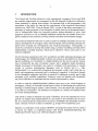
INTRODUCTION
The Finnish and Swedish radioactive waste management companies, Posiva and SKB,
are currently endeavoured in a programme for the safe disposal of high-level radioactive
waste generated by nuclear power plants. An important task in this programme is the
assessment of the safety for man and the environment of the proposed technological
solution (e.g. SKB 2004, Vieno & Ikonen 2005). As part of the safety assessment, it is
necessary to make prognoses of the biosphere evolution and the environmental behaviour of radionuclides under very long-term periods, lasting thousands of years. Such
prognoses will have to rely on multiple-interfaced models that can handle diverse biosphere conditions and scenarios involving climatic and other environmental changes.
The model development will have to involve experts in multiple disciplines and its continuous development is envisaged, which will incorporate new knowledge and data obtained from on-going site investigations and research programmes. Consequently, it
would be convenient to develop the models using a common modelling tool that allows
implementing a modular structure, which can be shared by various users and be continuously upgraded.
Several existing commercial codes were considered, and after analysing advantages and
disadvantages, the Matlab/Simulink© software was chosen as the platform for developing the modelling tool. Simulink© is a highly flexible tool that can be used for simulations of practically any type of dynamic system, with a graphical model description.
Models developed in Simulink© can easily be combined with procedures or models
written in common programming languages, such as Fortran and C++. Matlab/Simulink© is a commercially transparent environment, widely used within the scientific and engineering community and is continuously upgraded. A drawback, though,
is that substantial experience and effort is required to implement a model, and to take
advantage of all available capabilities. Moreover, users not familiar with Simulink©
may have difficulties to understand and run models implemented by others.
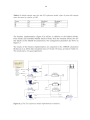
In order to make the Matlab/Simulink© platform more easy to use, whilst keeping its
advantages, a library of Simulink© blocks and a toolbox for facilitating the creation and
handling of radioecological models, called Pandora, were developed and implemented
as an add-on to Simulink©. The Pandora tool comprises of a library of Simulink blocks
and a free standing Manager.
This report is mainly a technical user guide of Pandora, but it also presents the tool in
general. An step-by-step implementation of a test model is also described for an example. It is assumed that the reader knows the basics of Matlab© and Simulink© environments. General overview on them is available e.g. at http://www.mathworks.com/.
Pandora is a unification of the projects BIOMAT developed by Facilia AB on contract
to Posiva Oy within a co-operation project with Svensk Kambranslehantering AB
(SKB) and TENSIT (Jones et al. 2004) developed by SKB.
4
5
2
PANDORA VERSION 1
The Pandora tool comprises of a library of Simulink blocks and a free standing interface, The "Pandora Manager", a utility to facilitate the implementation of radionuclide
transport models in Simulink.
The following parts, described in more detail in chapters 3 and 4, are included in the
Pandora (version 1.0) library:
• Radionuclide Manager (Pandora-block) - for handling decay and in-growth of
several radionuclides.
• Constant+ block- for easier handling of possibly nuclide-dependent parameters.
• Parameter manager- used in conjunction with Constant+ block for central editing of values and distributions.
• Reservoir - for creation of compartments that can easily handle multiple radionuclide decay and in-growth data.
• Rate block to be used with Reservoir blocks to control flux between Reservoirs.
• Filter block - to filter out certain nuclides, signal dimensions are preserved.
• Selector block -to select certain nuclides, signal dimensions are reduced.
• Result Report Manager- for exporting named data to text files and/or Excel.
• Plot Manager- for representing named data in Matlab plot windows.
• Parameter Report Manager - for exporting system settings and model parameters to text files.
• Unit conversion blocks "bq2mole" and "mole2bq" for conversion of units between mole and becquerel.
• Inflow block - to represent inflow of contaminants to the model.
• Statistics blocks - to define result nodes in the model, when running probabilistic simulation.
All codes in Pandora are written in the Matlab and Java languages. Java is used only
internally in Pandora and no knowledge of Java is needed to use Pandora. Some knowledge of Matlab is probably an advantage and basic knowledge of how to build blockbased models in Simulink is required to use Pandora. Although one could build simple
models (as the test case) with less experience, familiarity with Simulink is strongly recommended for making the simulation settings and connecting other non-basic blocks
than the Pandora blocks to the model.
6
7
3
PANDORA TOOLS
The Pandora tool consists of two separate parts: the Pandora Manager and the Pandora
library of Simulink blocks. The blocks in the library can be used independent of the
Pandora Manager but the Manager facilitates the construction and maintenance of large
models.
In this chapter, the Pandora Manager and controlling of model creation and simulation
runs are presented. Chapter 4 introduces then the actual building blocks of the Pandora
models, i.e. the block library.
3.1
Parameter handling through Excel sheets
The input of parameters in Pandora is done via Excel sheets. There are three different
types of parameters handled by Pandora:
• Site-specific: Scalar local parameters e.g. lake area.
• Element-specific: Nuclide-dependent, or in general species-dependent, global
parameters e.g. Kd.
• Universal: Scalar global parameters typically physical constants e.g. gravity.
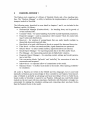
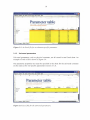
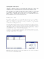
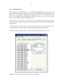
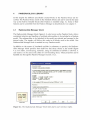
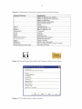
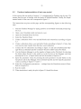
Parameters are stored in Excel sheets, which in turn are pointed to in a main Excel setup sheet for the model. An example of such a main sheet is shown in figure 3.1. The
contents of this sheet can either be edited directly in Excel or through the parameters tab
in the Pandora Manager (see section 3.3).
Site specific paranlters filename:
" comment
C : \md\egen_firma\facilia\te~t\test_mod~ l_§ i!e_Spec!.fi.£_P ~ ameters . xj s
Univers""il paranltersrue-nanle:
Ml comment
-
comment
IC:\md\ eqen firma\fac ilia\pandora\ pandora050531 \pandora\database\e xcel\universal\univ~My comment
Figure 3.1. Model set-up file (the main sheet) in Excel.
8
In the leftmost column (column A) of the Excel sheet tags can be found. These tags
must not be changed.
This sheet must be placed in the same folder as the model, and its name must be:
modelname_setup.xls where mode/name is the name of the model. The set-up sheet
must contain three fields:
• Site-specific parameters filename (section 3.1.1 ),
• Element-specific parameters filename (section 3.1.2),
• Universal parameters filename (section 3.1.3).
3.1.1
Site-specific parameters
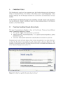
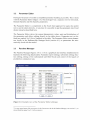
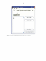
Site-specific parameters are stored in one Excel sheet per model. An example of such
file is shown in figure 3.2.
In the leftmost column (A) of the Excel sheet, a tag can be found (in fig. 3.2, Table-
Type _yaram_ vO 1). This tag must not be changed.
New site-specific constants can be added by inserting new rows in the sheet. The new
row must be inserted below the tag and above the STOP markers (in fig. 3.2, on line
14).
GJ[Q)(8]
""'\. Microsoft Excel - test_model_Site_Specific_Parameters.xls
Jl!:J t1rkiv
~edigera
]J D ~~ ~ ~C9.~ ]
J]
•
Arial
·IF
X
U = ==
-
a
0
----+""'-
11-
4
,..__ "''""'"-- -...£. _...... "' ~
11 ~
-rI
9
10
11
.,.."lbleTY,;:;f'_r>ilril!l! ~
12 - - - - - 13 r-
_
__
141- - - - -
15
16r-
*
1- -
~
.,n
·'
----r
-l---
ooo .$oo
.. o
~~
~~
:..: .:
- :--':--....;
-
-
-
A •
E
-
-
--
--.
---1
J
~
-
---
I
··-
·--
----
---
Element
- - - _L_
---
-
--
!SToP
STOP
I
1
~
-
J~
1 Blad3 I
!r-1
Figure 3.2. Excel file of the site-specific parameters.
---+--
-
11rnd norm(1 ,1)
2 l rnd norm(2,1)
normQ 11l
ISfoP
- =±_-_-
----:--
Pandora distribution
Deterministic value
I
--
-
----
_i!_e Kt)
-
_
--
.v
· I00
%
~ •
I
-
-
I
-
A.
I
--~--r=-------····--
~
•ll tr.'
Parameter - ----.,.-
l test_tl'l~~l . subsystem_ll<
I~ I ~ I ~ I ~1 1\ Blad 11 Blad2
Klar
t
(te llt)
,test model. subsystem. Kd
'test model. subsystem. epsilon
STOP
•
0
-- - -
--·-
-
_ ~ ftli.II..IL ¥' ltV.Il _1&1 ~ ..u~
7
8 -----
000
100
c
B
~ ~~ If iitllll lltr.'l tr"li
5
6
• -4) ]
--1 --- 1- - - · •
~· .U I ~
L {.
=I STOP
I
A
1
2
3
'"'"'·1 &9 1
1- - - m1~ %
~ ~ft~ l l()·
10
...J
E14
_ J OJ J ~
!nfoga Format ~erktyg Q.ata F!inster tiialp
Vi~a
I
\-
-
--
-rI
11-
:
-
1...
~
l r - !NUM r-r----1
~
9
The properties that can be specified for a parameter are the following:
• Parameter - the actual name of the parameter in Matlab workspace,
• Element - element for which the parameter is valid (if also a nuclide-dependent
parameter),
• Deterministic value - the value to be used in deterministic simulations,
• Pandora distribution- distribution to be used in probabilistic simulations.
For a deterministic simulation only Parameter and Deterministic value have to be specified. For a probabilistic simulation also the Pandora distribution have to be specified.
In Pandora version 1 the following distributions are supported (the Pandora distributions):
• rnd_ uniform(min, max) - uniform distribution
• rnd_triang(min, mode, max) - triangular distribution
• rnd_logtriang(min, mode, max) - logtriangular distribution
• rnd_norm(mu,sigma) -normal distribution
• rnd_lognorm(mu,sigma) - lognormal distribution
There is also a possibility to add other properties for the parameter in the Excel sheet for
information to the reader (e.g. Unit, Literature references etc.). Pandora will ignore such
properties.
3.1.2
Element-specific parameters
Element-specific (or nuclide- or species-dependent) parameters are stored in one Excel
sheet per parameter, all files stored in the same directory. An example of an Excel file
for an element-specific parameter is shown in figure 3.3.
The properties that must be specified for an element-specific parameter are:
• Parameter - the actual name of the parameter in the Matlab workspace,
• Element - element for which the parameter is valid,
• Deterministic value - value to be used in deterministic simulations,
• Pandora distribution- distribution to be used in probabilistic simulations.
In figure 3.3, a part of an excel sheet for an element-specific parameter called Kd_peat
is shown. In addition to the four mandatory properties above, this sheet has a number of
optional parameters for information to the user.
Note that for the element-specific constants one Excel sheet is needed for each parameter, and the name of the Excel file must start with the parameter name. In the example
of figure 3.3 the name of the parameter is KD _peat and thus KD_peat_R0228.xls is a
valid name for the Excel sheet, the rest of the file name indicating supplementary information for the user. All Excel sheets for Element specific parameters must be stored
in the same directory on the file system.
10
ES.Kd_peat
ES.Kd_peat
ES.Kd_peat
ES.Kd_peat
ES.Kd_peat
ES.Kd_peat
ES.Kd_peat
ES.Kd_peat
ES.Kd_peat
ES.Kd_peat
ES
ES
ES
ES
ES
ES
ES
ES
ES
ES
Fe
Co
Ni
Se
Sr
lr
Figure 3.3. An Excel file for an element-specific parameter.
3.1.3
Universal parameters
Universal parameters, such as physical constants, are all stored in one Excel sheet. An
example of such a file is shown in figure 3 .4.
The parameter properties that must be specified in the sheet for the universal constants
are the same as for site-specific parameters (section 3.1.3).
~~~~~~~~ ·~ _!_..
Enter a dash .. _.. for empty, not re~vant properties.
Save file be~re ~XJlOrlin_g_para!_!!eters!
(text)
Object
a'
~e3!1 _
....., Simulink path ""
lake
STOP
(18Jt!l
_.J!.§.:!L
Parameter
Type
UC.Tk
STOP
u
_ _..,..,s:o.o.
T.w..t
OP - - - - --FSTOP
Figure 3.4. Excel file for the universal parameters.
(te«t)Element
STOP
-+-
-,-
.(tex1
Unit
11
3.2
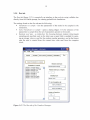
Parameter Editor
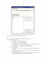
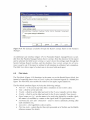
During development of models a simplified parameter handling is possible. This is done
with the Parameter Editor (figure 3.5). This dialoguea has a separate view for Universal,
Element Specific and Site Specific parameters.
The Parameter Editor is complement to the Excel sheet approach for users who prefer
not to use the sheets directly. At any time it is possible to put the parameters into Excel
sheets instead as described here.
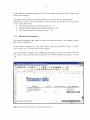
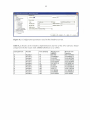
The Parameter Editor shows the current deterministic values, units and distributions of
the parameters and allows editing directly in the table shown. Parameters not yet defined are marked NaN (Not a Number) in the table. The Parameter Editor saves parameters locally in the Radionuclide Manager block (section 4.1) so parameters are automatically saved with the model.
3.3
Pandora Manager
The Pandora Manager (figures 3.6 to 3.15) is a graphical user interface implemented to
facilitate the following functionality: Parameter report settings, subsystem editing, function editing, editing of the radionuclide and filter blocks and control of the launch of
probabilistic simulation runs.
~
GJLQJ1!8]
Parameter Editor
Tools
Element Specific Parameters
Name
Kd coast - Cl-36
Kd coast - Ni-59
Kd coast - Tc-99
Kd coast - 1-1 29
Kd coast - Cs-1 35
Kd coast - Ra-226
Kd coast - Pu-239
Kd coast- Am-241
Kd lake - Cl-36
Kd lake - Ni-59
Kd lake - Tc-99
Kd lake - 1-1 29
value
0.0010
10.0
0.1
0.3
10.0
10.0
100.0
10.0
1 .0
10.0
0.1
0.3
,...,,...,
Unit
m311<g
m311<g
m311<g
m311<g
m311<g
m311<g
m311<g
m311<g
m311<g
m311<g
m311<g
m311<g
1
Distribution
rnd logtriang(0.0001,0.001, ... A
rnd logtriang(1,1 0,1 00)
rnd logtriang(O.o1,0.1,1)
rnd logtriang(0.1,0.3,1)
§]
rnd logtriang(1,1 0,1 00)
rnd logtriang(1,1 0,1 00)
rnd logtriang(1 0,100,1 000)
rnd logtriang(1,1 0,1 00)
rnd_logtriang(0 .1,1,1 0)
rnd logtriang(1,1 0,1 00)
rnd logtriang(0 .01,0 .1,1)
rnd logtriang(0.1,0.3,1)
,,...,
·"A
Apply
I[
Parameter Type -
0
Universal
G> ~!~~~~if§P.:~:~:(!):s
0
Site Specific
V
Close
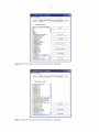
Figure 3.5. Example view of the Parameter Editor dialogue.
To open, press button Edit parameters in the Parameters tab in the Pandora Manager, see section 3.3, or
choose from the menu Tools> Edit parameters.
a
12
•1
G]lu
Pandora Manager: olkiluoto
File
Tools
Report
~
Help
11 Nuclides 11 Subsystems!! Functions 11 Parameters 11
Run
List:
~ Result-Report blocks
~ Plot-Manager blocks
Plot
Plot1
Plot2
Plot I View table
Set no. of inputs
Report settings
V
System settings to report
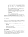
Figure 3.6. The Report tab of the Pandora Manager.
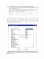
The Pandora Manager has three menus that are always visible:
• File menu containing:
o New Model- to create a new model,
o Open Model - to open an existing model,
o Save Model - to save the current model,
o Save parameters - to save the parameters and nuclide information (selected nuclides and decay chains) to a separate file,
o Load parameters - to load previously saved parameters.
• Tools menu containing:
o List Equations - shows a list of the differential equations represented by
the model,
o Open project file - opens the main Excel set-up sheet with links to the
parameter files (figure 3.1 ),
o Import project file - opens a file selection dialogue to import a project
file from another project or elsewhere on the file system,
13
Load params from Excel - load the parameter values defined in the Excel
sheets (sections 3.1.1 to 3.1.3),
o Export Nuclide Chain to .xis file - to export nuclide chains to an Excel
file,
o Import Nuclide Chain from .xis file - to import a chain from an Excel
file,
o Clear Cache - clears the intermediate Matlab files created from the Excel
sheets; this is normally not necessary since the intermediate files are updated automatically when an Excel file is changed,
o Create Excel templates for undefined parameters - creates automatically
a template for the parameter file and for files of the site-specific parameters (for a newly created model),
o Edit parameters- opens the Parameter Editor (figure 3.5) for local editing of parameters.
Help menu containing:
o User Guide - opens the Pandora User Guide,
o About - gives some information about Pandora version currently used.
o
•
In addition to the menus, the Pandora Manager user interface has the following six tabs
discussed in detail below: Report, Nuclides, Subsystems, Functions, Parameters, and
Run.
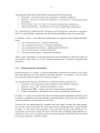
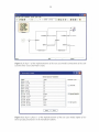
3.3.1
Report tab
In the Report tab (figure 3.6) the controls for reporting the results are located. In the list
box to the left, the blocks supporting the Plot block (section 4.6) and the Result Report
blocks (section 4.5) are listed. By double-clicking one of the items in the list box the
corresponding user interface for the block is opened.
On the right side of the Report tab, the following pushbuttons are located:
• Plot I View table - shows a plot from a Plot block or opens a table with the results in Excel,
• Set no. of inputs - sets the number of inputs of a Plot or Result Report block,
• Report settings - opens the mask for the Parameter Report block in the model
(described in detail in section 4.5),
• System settings to report - allows selection of the simulation settings to be reported (described in detail in section 4.5).
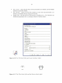
3.3.2
Nuclides tab
The Nuclides tab (figure 3.7) of the Pandora Manager controls the nuclides in the
model. As with the parameters (section 3.1 ), also the handling of the nuclide information is based on Excel sheets with partial complementary handling options through the
user interface of the Pandora Manager. In the list box to the left of the dialogue the nuelides present in the model, and their half-lives in years are shown.
14
r;]!u LE]
) Pandora Manager : olkiluoto
File
Tcols
Report
Help
11 Nuclides 11 Subsystemsjl Functions 11 Parameters 11
I
Run
Nu cl ides in model with halflives [Years]
3.01 e+005
Cl-36
Cs-135 2.3e+006
1-129 1.57e+007
Mo-93
4000
Ni-59
76000
Np-237 2.144e+006
Pu-239 24110
i~
~~
[
Add nuclide
]
[
Remove nuclide
I
(
Select/sort nuclides
)
[
Edit Excel database
)
[
Update database
]
[
Edit Decay Pairs
)
Figure 3. 7. The Nuclides tab of the Pandora Manager.
The Nuclides tab has six pushbuttons:
• Add Nuclide - opens a dialogue to add a nuclide to the model,
• Remove nuclide- opens a dialogue to remove a nuclide from the model,
• Select/sort nuclides - opens a dialogue to change the order of the nuclides in the
model and in the reports,
• Edit Excel database - opens the Excel sheet containing the nuclide information
(see below),
• Update database - synchronises the nuclide information between the Pandora
Manager and the Excel sheet containing the nuclide information,
• Edit Decay Pairs- opens a dialogue to edit decay chains in the model (see below).
15
Defining of the nuclide half-lives
The input of half-lives is done in an Excel sheet called haljlifesXXX.xls (where XXX
stands for any text) in the Element Specific parameters directory on the file system.
Once the half-lives for a number of nuclides are specified in this file they can be loaded
to the model by pressing the Update database button in the Nuclides tab (figure 3.7).
When a nuclide is selected in the model the name of it is stored in the Radionuclide
Manager block (section 4.1 ), and saved with the model.
Handling of decay chains
Decay chains can be defined in the model. This information is saved in the Radionuclide Manager block (section 4.1), and thus saved with the model. There is also a possibility to store the decay chain information externally in Excel sheets, comparable to the
model parameter handling (section 3.1).
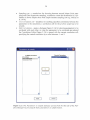
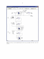
The Chain Editor in figure 3.8a shows the decay ofnuclides into each other by a branching decay for each pair. For example, in the figure, Nuclide 1 decays both into Nuclide 2
with branching ratio of 0.3 and into Nuclide 3 with branching ratio of 0. 7. Nuclide 2
decays further into Nuclide 4 with a 100% branching ratio.
A new decay pair can be created by pressing the Add Pair button of the Chain Editor,
resulting a dialogue (figure 3.8b) to appear
~
LJ[g] ~
Chain Editor
I Daughter
Nuclide 2
Nuclide
Nuclide 1
Ratio
0 .3
Nuclide 1
Nuclide 3
0 .7
Nuclide 2
Nuclide 4
1 .0
~ Input Pair
LJ[§ ~
Parent j U-234
I
Daughter Th-230
vI
v I
I
Ratio j 1 .0
I
Apply
11
Cancel
l(
Add Pair
)11 Remove Pair . ,)
[
Apply
)I
Cancel
j
Figure 3.8. a) The Chain Editor dialogue (left), b) The Input Pair dialogue for adding a
decay pair from the Chain Editor (right).
16
This Input Pair dialogue contains three fields that select the parent, the daughter and the
branching factor for the decay pair. Selection of the parent and the daughter is implemented by using the drop down lists. The branching ratio can be typed as a number between zero and one. The drop down lists contain only the nuclides present in the model;
before creating a decay chain, the needed nuclides need to be added to the model. After
adding a new pair, the branching ratio can be edited directly in the Chain Editor by double clicking on the ratio field and typing in new branching ratio.
To remove a pair, the decay pair to be removed is selected by clicking any of the fields
of the decay pair, and clicking the Remove Pair button of the Chain Editor.
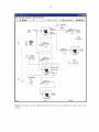
3.3.3
Subsystems tab
The Subsystems tab (figure 3 .9) of the Pandora Manager helps to find and edit the subsystems in the model. In the list box to the left of the dialogue the subsystems in the
model are shown. It is also possible to only show the Pandora subsystems with the tick
box above the list, resulting in omitting the other (elementary) Simulink blocks from the
list. A listed block is shown in the model by clicking its name.
The Subsystems tab has the following buttons:
• Open - to open the selected subsystem,
• Remove Image - to remove an image on the selected block,
• Set Image - to set an image on the selected block (for details, see the Simulink
documentation on putting an image on a subsystem),
• Set out-sig. names - to propagate names of Out ports to connected lines,
• Terminate outputs -to terminate unconnected Out ports to avoid warning messages when running simulation,
• Constant inputs - to connect a Constant+ block to unconnected In ports; the
name of the Constant+ block is taken from the port name,
• Ground inputs - to connect a Simulink ground block to unconnected In ports.
For further description of the functions of the Subsystems block, see the implementation
description of the test in chapter 5.
3.3.4
Functions tab
The Functions tab (figure 3.10) of the Pandora Manager lists all the Function blocks
(section 4.4) used in the model. The buttons of the tab are:
• Add input - adds a new input to the function,
• Constant inputs- connects a Constant+ block (section 4.3) to the unconnected In
ports (the name of the Constant+ block is taken from the port name),
• Ground inputs - connects a Simulink ground block to unconnected In ports.
17
•1
GJ ~ r:l ~
Pandora Ma nager: olkiluoto
File
Tools
Report
~
Help
11 Nuclides 11 Subsystemsjl Functions 11 Parameters 11
Run
Subsystems in model:
~ Show only Pandora subsystems
Plot
Plot1
Plot2
,.~
Release
TENSIT
coast!Bay JBayDeepSediment
coast!Bay JBaySediment
coast!Bay JBayWater
coast !Bay!Depth
coast!Bay!Dm
coast !Bay ll<d_sea
coast !BayJleveiToConc
coast!Bay !M sed
coast!Bay IRETTIME
coast!Bay ISR
coast!Bay ISusp
coast!Bay fTCbo
coast!Bay fT Csd
coast!Bay fTCsw
coast !Bay fT Cws
coast !Bay la
coast!Bay !block to changeline color
coast !Bay!block to changeline color
.~
coast!Baylk
( tl
IU
)j j
Open
Remove Image
Set Image
Set out-sig. names
Terminate outputs
Constant inputs
Ground inputs
Figure 3.9. The Subsystems tab of the Pandora Manager .
~[ u
.I Pandora Manager : olkiluoto
File
Tools
Report
11 Nuclides 11 Subsystemsll Functions 11 Parameters 11
Function blocks in model
coast!Bay JleveiT oConc
coastJBayfTCbo
coast!BayfTCsd
coast!Bay fTCsw
coast!Bay fTCws
coastiSeafT Cob
coastiSeafT Cof
coastiSeafTCsd
coastiSeafT Csw
coastiSeafTCws
forestlfaunalmoose/CR_H_moose
forestlfaunalmoose/C _diet_moose forest/fauna/moose/cone moose
forest/fauna/roe deer ICR_H_roede
forest/fauna/roe deer IC_diet
forest/fauna/roe deer /cone _roede
forest/soilfTC _S2L
forest/soilfTC _S20ut
forest/soilfTC _S2U
forest/soilfTC _sm
forest/soil/area scaling1
forest/soil/area scaling2
forest/soil/cone soil
V
forest/soil/flux Li2So
<,
l8J
~
Help
.~
>tl
=
Add input
Constant inputs
Ground inputs
Figure 3.10. The Functions tab of the Pandora Manager.
Run
18
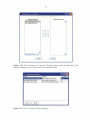
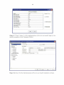
3.3.5
Parameters tab
The Parameters tab (see figure 3.11) of the Pandora Manager has two list boxes. The
left one lists all Constant+ blocks (section 4.3) in the model and the right one lists the
paths to the Excel sheets containing the parameters (section 3.1). The Excel path list
box does not update automatically due to the long access time to the sheets; instead
there is a button Refresh file list to update the list.
A single click in the left list box will show the corresponding Constant+ block in the
model. A double click in the left list box will open the Excel sheet with the corresponding parameter.
A double click in the right list box will lets select new files for the site-specific or universal parameters or a new directory for the element-specific parameter files.
The Edit parameters button opens the Parameter Editor described in section 3 .2 .
Pandor a Manager : landscape_year _2020_AD
.l
File
Tools
Report
11
Nuclides 11 Subsystems!I Functions 11 Parameters 11
Lake _ID _22~ake _v02..0X
Lake _ID _22~ake _v02..0s
Lake _ID _22~ake _v02.1F racX
Lake _ID _22~ake _v02/Gs
Lake _ID _22~ake _v02.1Kd_lake
Lake _ID _22~ake _v021RETTIME
Lake _ID _22~ake _v021SuspX
Lake _ID _22~ake _v02ffk
Lake _ID _22~ake _v02Nadv
Lake _ID _22~ake _v02Nsink
Lake _ID _22~ake _v02/area
Lake _ID _22~ake _v021porosity
Lake _ID _22~ake _v02/rho
Lake _ID _23/lake _v021DX
Lake _ID _23~ake _v02..0s
Lake _ID _23~ake _v02.1FracX
Lake _ID _23~ake _v02/Gs
Lake _ID _23~ake _v02.1Kd_lake
Lake _ID _23~ake _v021RETTIME
Lake _ID _23~ake _v021SuspX
Lake _ID _23/lake _v02ffk
Lake _ID _23~ake _v02Nadv
Lake _ID _23~ake _v02Nsink
Lake _ID _23~ake _v02/area
I Ak'P. If) ?1J1Ak'P. vn? lnnrn:c:::itv
llll
1
Run
1
Project parameter files
Constant+ blocks in model
<
l;JIQ ~
Help
-
SiteSpecific
: C: 'lmd\eg~ ;..
Universal
ElementSpecific : C: 'lmd\eg€
>JI
Refresh filelist
>~
Jl
L___-.;.._.JJ
_
Edit parameters
Figure 3.11. The Parameters tab of the Pandora Manager.
.
19
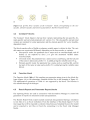
3.3.6
Run tab
The Run tab (figure 3.12) is essentially an interface to the probsim script, callable also
directly from the Matlab prompt, for running probabilistic simulations.
The settings found on the Run tab are the following:
• Parameters to sample - lists the parameters of the model to be sampled in the
simulation,
• Select Parameters to sample - opens a dialog (figure 3.13) for selection of the
parameters to sample from the set of parameters present in the model,
• Random seed type - a combo-box for choosing between random (time-based)
sampling and specified seed; in the latter case a input field is enabled for entering an integer value as seed for the random number generator, and in the former
case the seed is created from the current time value read from the computer
clock,
G]lC
) Pandora Manager : olkiluoto
File
Tools
Help
Run
Report
Select Parameters to sample
Random seed type:
Parameters to sample
olkiluoto .coast .Bay .Msed
olkiluoto .coast .Bay .RETTIME
olkiluoto .coast .Bay .SR
olkiluoto .coast .Bay .Susp
olkiluoto .coast .Bay .a
olkiluoto .coast .Bay .k
olkiluoto .coast .Sea .Depth
olkiluoto .coast .Sea .Msed
.;...
IRandom(time based)
J
Random seed (pos. integer):
Sampling type:
IMonte Carlo
D Use Correlation cell
(
Edit Correlations
(
Clear Correlations
Number of iterations:
10
V
Figure 3.12. The Run tab of the Pandora Manager.
Run
~
20
•
Sampling type - a combo-box for choosing between normal Monte Carlo sampling and Latin Hypercube sampling, a method to create the distribution of a parameter in fewer samples than with simple random sampling (see e.g. McKay et
al. 1979),
Use Correlation cell - checkbox for enabling specified correlations between the
parameters in the simulation; a correlation cell for the probsim script has to be
created,
Edit Correlations- opens a dialogue (figure 3.14) for selecting parameters to be
correlated with each other, or when the parameters to be correlated are selected
the Correlations Editor (figure 3 .15) is opened with the current correlation cell,
specifying the wanted correlation by a value between -1 and 1.
•
•
.I
r;]lu
Parameters to sample
Available parameters
ES .initstate
est_modei.TCab
est_modei.TCba
~
Selected Parameters
A
test _rnoc~el . TCab
V
Apply
V
Cancel
Figure 3.13. The Parameters to sample dialogue opened from the Run tab of the Pandora Manager by pressing the Select parameters to sample button.
21
•
1
~ I u ,[8]
Parameters to correalate
Selected Parameters
Available parameters
~ ~~st_model.subsystem.Kd ~,~
est_model.subsystem .epsi est_model .subsystem .tk
<<
<Jl
ll!l.
V
Apply
Cancel
Figure 3.14. The Parameters to correlate dialogue opened from the Run tab of the
Pandora Manager by pressing the Edit correlations button.
Apply
) (
Cancel
Figure 3.15. The Correlations Editor dialogue.
23
4
PANDORA BLOCK LIBRARY
In this chapter the different specifically created blocks in the Pandora library are described. The Pandora blocks reside in the Simulink library and can be used in the same
way as the built-in Simulik blocks after Pandora is installed (App. A). Some of their
features can be controlled from the Pandora Manager as described above in chapter 3.
4.1
Radionuclide Manager block
The Radionuclide Manager block (figure 4.1), also known as the Pandora block, allows
centralised selection and handling of multiple radionuclides to be included in a Pandora
model. The radionuclides to be included in the model are selected and arranged to the
desired order. The signals will follow this order in all blocks used in the model. One
Radionuclide Manager block is needed in every Pandora model.
In addition to the names of simulated nuclides (or elements or species), the Radionuclide Manager block specifies their half-lives and decay chains in the model (figure
4.1). For stable, non-decaying, materials, using Inf (infinite) as half-life is allowed. A
zero matrix is to be used as the chain for non-branching decay. These properties can be
handled also through the Pandora Manager (section 3.3.2).
~
~ Block Parameters: PAt,mORA
r- Subs_ystem (mask)
Needed in every pandora simulation.
A pandora block specifies names of simulated elements, their halflifes and decay
chains. For stable non decaying materials, use "inf" as halflife. Use a zero matrix
as chain for non branching decay.
Exanple:
NAMES
HALFLIFE
CHAIN
={'U-234';
'Th-230'; 'H20';}
=[ 145500 75380 inf]
=[ 0 0 0; 1 0 0; 0 0 0; 1
In this example U-234 decays and braches (1 00%) into Th-230.
r-
Parameters
Nuclide names (string) [NAMES]
j{'U-234'; 'Th-230'; 'Ra-226';}
Nuclide halflife (year) [HALFLIFE]
1[245500;75380;1600]
U-234 _246500
Th-230 75380
Ra-226 1600
PANDORA
Decay chain (year) [CHAIN]
hoo0;1 oo;o 1 01
I
.QK
I
.Cancel
I
.t!elp
I
8:pply
Figure 4.1. The Radionuclide Manager block (left) and its user interface (right).
I
24
in
Reservoir
Rate
Figure 4.2. The Reservoir block (left) and the Rate block (right).
In any Pandora model it is possible to include only one Radionuclide Manager block.
When doing this, decay and in-growth data, as well as the names of the selected radionuclides become available throughout the entire model. The names of the radionuclides are not transferred in the model, but are instead read from the Radionuclide Manager. There is, therefore, no need or possibility to connect the Radionuclide Manager
block with other blocks in the model.
4.2
Reservoir and Rate blocks
The Reservoir block (figure 4-2) has one In port representing incoming flux to be integrated. The Reservoir block corresponds to a compartment in the classical conceptual
transport models. The first Out-port is level signalling the current level of integration.
The remaining Out ports are flux-out ports. They are designed to be connected only to
the Rate block (figure 4-2) controlling the outflow from the Reservoir block.
The Rate block is meant to control outgoing flux from Reservoir blocks. A flux-out port
from a Reservoir is connected directly to the centre In port of the Rate block. A signal
carrying the transfer rate coefficient (typically from a Function block, see section 4.4) is
connected to the rate port, and then the outgoing flux of the Reservoir block is controlled by the rate signal through a hidden backward connection to the Reservoir block.
The Rate block with a given rate corresponds to a transfer (expressed as a transfer coefficient) in the classical conceptual transport models.
The third In port in the Rate block is for symmetry only and can be left unconnected or
connected to a Simulink ground block.
The half-life vector (HALFLIFE) and decay matrix (CHAIN) specified in the Radionuclide Manager block are available in the Reservoir block. The decay is calculated according to the formula
dY
-=C·YA--YAdt
(4.1)
where Y is the vector of nuclide levels, C is the CHAIN matrix, A is ln(2)/HALFLIFE,
and YA denotes element wise multiplication of Y and A.
25
.......-~.....
/ unde\ fined 1
'~-. ____., /
~~]
[
''j
C:(.
t r
t
u1
---,
u2
trned
u3
..~P
• 1.,
b)
a)
-
";tro rr
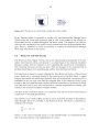
Figure 4.3. a) The three variants of the Constant+ block corresponding to the sitespecific, element-specific and universal parameters. b) The Function block.
4.3
Constant+ blocks
The Constant+ block (figure 4.3a) has three variants representing the site-specific, element-specific and universal parameters (cf. section 3.1). The site-specific and universal
variants are intended for scalar parameters and the element-specific for vector (nuclidedependent) input.
The block searches after a Matlab workspace variable name to obtain its data. The variable names are constructed differently depending on the three modes, or variants:
• Site-specific mode: the parameter has a name such as coast/bay/depth, and all
slashes (/) are replaced by dots (.) to give the structured variable name:
coast.bay.depth,
• Universal mode: the parameter has a name such as coast/bay/g, and the last part
of the name is taken and a prefix UC. is added giving the variable name UC.g,
• Element-specific mode: the parameter has a name such as coast/bay/Kd, and the
last part of the name is taken and a prefix ES. is added giving the variable name
ES.Kd.
4.4
Function block
The Function block (figure 4.3b) translates an expression string given in the block dialogue (figure 4.4) to the elementary Simulink blocks like in the example of figure 4.5.
The mathematical operations of Table 4.1 are supported by the block. The function is
also editable through the dialogue.
4.5
Result Report and Parameter Report blocks
The reporting blocks are used in connection with the Pandora Manager to control the
generation of reports on simulation results and parameters.
The Results Report block exports named numerical data generated during a simulation
to text files or to an Excel worksheet. From the interface of this block (figure 4. 7), the
time range that will be exported is selected. Data from any Simulink block in the model
can be exported to text files or Excel (by connecting it to the Excel Link Manager
block).
26
l;JI0 (g)
.~ Edit function expression
Available
+
.I
1unctions ---------------------~
- 1\olatnx ot elementw1se addition
Matrix or elementwise subtraction
Matrix multiplication
Element-wise multiplication
- Element-wise division
V
Available
Inputs ----------------------~
u2
u3
[ Add new input
I
~xpression.
u1+ u2 + u3
[ (
Apply
J
[
Cancel
I
[..___c_le_ar_ ..J
Figure 4.4. The Function block dialogue.
This bloc/f.
tr;~nslates
the expression
A."B+C .l D
to the elementary simulin/f. blocl<s seen below
Q1_2
8
c
Subexp1
Q1_3
D
Figure 4.5. Example of the system of elementary Simulink blocks created by the Function block.
27
Table 4.1. Mathematical operations supported by the Function block.
Explanation
Operator/Function
+
Matrix
or element-wise addition
····-···-································· ·······································································-················································································································································································································································································
Matrix
or element-wise subtraction
...................................................................................................
. .*. . . . . . . . . . . . . . . . . . . . . . . . . . . . . . . . . . . . . . . . . . . .
.··· · · · · ···· · · ······ · ·..: JY.t~!d~:: ~:~HIP.:H~:~!!2.:6.:·-:···: : :~·: : :··:·:·: : : : : : ::· · · ·· ·· · · · · · · · ·
·: ·: :::.: : : :·: ··:: : ·: ·::··
•....*. ............... . . . . . .. . . . . . . . . . . . .. . . . . .. . . . . . . . . . . . . . . . . . . . . . . .. . . .. . . .................. ..............................~.l.~. ~. ~.~.!:~i.~.~. .~. ~.l.!.i.P.I.!. ~.?!.i9..~. . . .
........ .. .. .. .. ... .. ..... .. ... .. .
./....... . ....... . . . ....... . ............ ........... ....... . . . . . ............... . . ....... ....... . ................
Element-wise
...A
. .F>.
owe·;:..
.division
. . . . . . . . . . . . . . . . . . . . . . . . . . . . . . . . . . . . . .... .. . . . . . . . . . ...... . . . . . . . . . . . . . . . . . . . . . .
.....................................................................
.................................................................................................................................................................................................................................................................................................... ..................................
. .§qr~H...~.l.. . . . . . . . . . . . . . . . . . . . . . . . . . . . . . . . . . . . . . . . . . . . . . . . . . . . . . . . . . . . . . . . ....§.9 .~.9.T.~t.9..9.!...9.f...~. . . . . . . . . . . . . . . . . . . . . . . . . . . . . . . . . . . . . . . . . . . . . . . . . . . . . . . . . . . . . . . . ..... . . . . . . . . . . . . . . . . . . ..
. .!.9..9(. .~.>. . . -. . . . . . . . . . ..
. ... . . ... -.. . . . . . . . ... . . . . . . . ... ... . . . . . .. .N. ?.!~.~.9..!. ..!.C?..9.?..~i.!.h.~. . 9.f.. .~... . . . . . . ... . .. . . . . .
. . . .. .. . .. . . . . . . . ...
. .!.9..9.1. 9..(. .~1... . . .... . . . . . . . . . . ..... . . .. . . . . . . . . . . . . . . . . . . . .... . .... . . . . . . . . . . . . . ..~.?..§.~. . 1. 9. . !.9..9.9.T.iJh.~. ...9.f...~
. . ... . ... . .. . . ..... . .
. .!r?..Q.§.P..!?..~ .~(~J. . . . . . . . . . . . . . . . . . . . . . . . . . . . . . . . . . . . . . . . . . . . . . . . . . . . . . ....!.~?.Q .§.P.9.~.~ . . .
. . . . . . . . . . . . . . . . . . . . . .. ..... . . . . . . . . . . . . . . . . . . . . . . . . . . . . . . . . . . . . . . . . . . . . . . . . . . . . . . . . .
. .!.Q.Y..L~J.. . . . . . . . . . . . . . . . . . . . . . . . . . . . . . . . . . . . . . . . . . . . . . . . . . . . . . . . . . . . . . . . . . . . . . . .J.Q.Y..~r.§.~. . . . . . . . .
.... ...... ........ .
. .~~. P.(~). . ...... . . . . . . . . . . . . . . . . . . . . . . . . . . . . . . . . . . . . .. . . . ........ . . . . .. . . . . . . . . . . .....~.~.P..9..~. ~.Q.t. . . . . . . . .. . . . . . . . . . . . . . . . . . . . . . . . . .
. .?..~~(~).. . . . . . . . . . . . . . . . . . . . . . . . . . . .. ......................................................
. A.9..§.9..!.~. !~. . Y9.J..Y..~. . . . . . . . . . . . . . . . . . . . . . . . . . . . .
.. . . . . . .. . . . . . . . . . .... . . . . .. . . . . . . . . . ..
. r~. ~.{~.~.Yt.~. . ~.9.9.{~.~. Y1
....... . . . . . .....R~.r:D.?.J..~.9 .~.r.. . ?..~.9.. }n.. C?..9. ~J.~.§. . . . . . . . . . . . . . ............ .. . . . . . . . . . . . . . . . . . . . . . . . . . . .
. .~.!. ?.:.~. <.==..~.?.:.:=..~.=:.:=. ~.:.:=.. . . . . . . .
............ . .R~I.?.~J.9.Q.?.L..9..P.~.~.9..!.i.Q. Q.§... . . . . ......................................... . . . . . . . . . . . . . . . . . . . . .. . . ... . . . . . . . . . . . . . . ..
. .§J.9.Q{~). . . . . . . . . . . . . . . . . . . . . . . . . . . . . . . . . . . . . . . .. . . . . . . . . . . . . . . . . . . . . . . . . . . . . . .§J.9.Q.~. r:D. . f~.Q .~.!.i.9..~...... . . . . .. . . . . . . . . . . . . . . . . ..........
. .9. ~J..9..Y(~.~..YJ......... . .. . . . . . . . . . . . . . . . . . . . . . . ................... . . . . . . .. . . . . . . . . . . . . .Q~I..9..Y. .~. ."'Y..i.!.h. ..Y.. !.i..r:D.~.:~!~. P..§. . ........ .. . . . . . . . . . . . . . . . ......................................................... .
. .~. ?!~.~. r:D{~1.. . . . . . . . . . . . . . . . . . . . . . . . . . . . . . .. . . . . . . ........... . . . . . . .....................§.~.~. J.h.~. . ~9.."'Y.~. .9.f. .~. ?.!.f.i.~. .~. {~~!~E.~.~. .Y~g!QE2.... . . . . . . . . . . . . . . . . . . . . . . . . . .
floor(x},ceil(x},round(x},fix(x)
Rounding functions
Parameter
Report Manager
Result Report
Figure 4.6. Result Report block (left) and Parameter Report block (right).
~
~ Sink Block Parameters: Result Report
~ Subsyslem (mask)
Export Result to text files, Export data to Excel
I
,- Parameters
r:~~9r~ ~oXx~~~ ~~~ ~
P'
Write to file
Report Directory
I. / report/result
Signal name Port 1
Isubsystem.Levelt..
Signal name Port 2
lsubsystem.LevelS
Sample Time (-1 for inherited)
l-1
I
QK
I
.Cancel
Figure 4. 7. The Result Report block interface.
I
.l::!elp
I
~pply
I
28
The result-report block user interface (figure 4.7) has the following settings:
• Export to Excel now - used at any time after a simulation has been run to list the
simulation results in Excel,
• Write to file - to choose if the results are written to a text file (normally set on
when doing probabilistic simulations generating several result files),
• Report Directory - to set the report directory,
• Signal name port [x] - sets the name to be used in the report for a certain signal;
this name is overridden by a name on the signal itself if a signal name is set,
• Sample time - sets the interval of reported values, normally set to -1 for inherited, see the Matlab documentation for to-workspace block for further details.
The System Settings Report interface (figure 4.8) is a part of the Parameter Report manager/block available from the Pandora Manager button System settings to report. The
left list box shows all the available system settings, and the right one the settings selected by user to be reported (by pressing the > > button). The default settings selected
automatically are shown in figure 4.8 .
•
1
l;JILl ~
System settings to report
System settings to report
System settings
A
Name
Tag
Description
Type
Parent
Handle
HiliteAncestors
Requirementlnfo
SavedCharacterEncoding
Version
MdiSubVersion
Preloadfcn
Postloadf en
Block Diagram Type
Library Type
SaveDefaultBiockParams
Sample TimeColors
LibrarylinkDisplay
Wdelines
ShowlineDimensions
ShowlineDimensionsOnErr
ShowPortData Types
ShowPortData TypesOnErrc
ShowloopsOnError
lgnoreBidirectionallines
V
~h ..... , .. ,cy,....,...,"'""rtac-c-
(
1
<<
SirnulationMode
Solver
SolverMode
Start Time
Stop Time
MaxStep
MinStep
MaxNumMinSteps
Initial Step
Fixed Step
ReiTol
AbsTol
MaxOrder
Solver Type
>1
Apply
V
Cancel
Figure 4.8. The System Settings Report interface of the Parameter Report block with
the default selection.
29
L.::: Block Parameters:
~
Parameter Report
- Subsystem (mask)
Export Result to text files, Export data to Excel
- Parameters
Report Directory
!tm!lDil&!dli¥Ja~aJll
System settings to report
JxNumMinSteps'; 'lnitiaiStep'; 'FixedStep'; 'ReiTol'; 'AbsTol'; 'MaxOrder'; 'SolverType'}
r
save system settings for all iterations
Note
Jnote
to report
I
.QK
I
ban eel
I
.t!.elp
i
8pply
J
Figure 4.9. The dialogue available through the Report settings button in the Pandora
Manager.
An additional user interface (figure 4.9) for Parameter Report manager/block is available from the Pandora Manager button Report settings. Here the directory for the report
can be selected, the field System settings to report shows the settings made through the
System Settings Report interface, and the checkbox Save system settings for all iterations is used to set if the report is written for all iterations in a Monte-Carlo simulation.
The field Note allows input of a short note to be saved with each report.
4.6
Plot block
The Plot block (figure 4.1 0) functions in the same way as the Result Report block, but
instead of exporting data to text or Excel, it plots the connected signals in a Matlab plot
figure. The Plot block also enables the control of line types, legend names etc.
The Plot block interface (figure 4.1 0) has the following settings:
• Plot now - to be used at any time after a simulation is run to draw a plot,
• Title - a field to set the plot title.
• Y-lable - a field to set the label and unit for theY -axis, typically Activity [Bq],
• X-lable- a field to set the label and unit for the X-axis, typically Time [years],
• Signal name port [x] - sets the name to be used in the legend for a certain signal;
this name is overridden by a name on the signal itself if a signal name is set,
• Automatically plot after simulation - used to choose automatic plotting after
each simulation run,
• Log scales - sets logarithmic scales in plots,
• Plot line-styles - selects the plot line style presented as in Matlab, see the Matlab
reference manual for details,
30
•
•
•
Plot colours- selects the plot line colours presented as in Matlab, see the Matlab
reference manual for details,
Plot markers - selects the plot line markers at each time step presented as in
Matlab, see Matlab reference manual for details,
Sample time - sets the interval of plot points, normally set to -1 for inherited, see
Matlab documentation for to-workspace block for further details.
(8]
~ Sink Block Parameters: Plot
~ Pk>t Manag" [m.,kJ
_ Export numerical data to matlab graph.
I
- Parameters
r ~~l~t:n~~]
Title
jBiosphere simulation
Y·lable
!Activity [8 q)
X·lable
jTime (year)
Signal name Port 1
Isubsystem.Level6.
Signal name Port 2
Isubsystem.LevelS
r
Automatically plot after simulation
P'
Log scales
Plot line·styles
I{'.'}
Plot colors
j {'b' 'g' 'r' 'c' 'm' 'y' 'k'}
..:J
..:J
Plot markers
I {':}
iJ
Sample Time (·1 for inherited)
1·1
I
Plot
OK
I
~ancel
I
Help
Figure 4.1 0. The Plot block (left) and its user interface (right).
>
Th-230
U-233
Filter
>
Selector
Figure 4.11. The Filter block (left) and the Selector block (right).
I
,6,pply
I
31
Cs-137 30
Th-230 75380
U-233 159200
TENSIT
9 .6851
9 .7461
Selector
Display1
P•nameter
Report Manager
9 .6851
9.7461
Filter
Display2
Result Report
Figure 4.12. Example of the use of Filter and Selector blocks.
4. 7
Filter and Selector blocks
The Filter block simplifies the implementation of models with different transfer functions for different nuclides, by setting the value of the unwanted nuclides to zero. The
Selector block is similar to the Filter block but the unwanted nuclides are removed totally from the signal vector, thus the signal dimension is reduced in a selector. Note that
Pandora cannot keep track of the nuclide names after a Selector block, this is up to the
user.
The example in figure 4.12 illustrates the use of filter and selector: For Display 1 we
have used a selector and thus we have reduced the dimensionality of the signal vector to
hold only the selected signals. The use of the filter block is illustrated with Display2
showing that the dimensionality of the signal vector is preserved and the values for the
unselected nuclides are set to zero.
4.8
Unit conversion blocks
The unit conversion blocks (bq2mole and mole2bq) provide conversion from activity in
Becquerel to amount of substance in mole and vice versa, according to the equations
32
Mole = Bq · HALFLIFE · 60 · 60 · 24 · 365
ln(2) · N A
(4.2)
B _
Mole · N A · ln(2)
q - HALFLIFE· 60 · 60 · 24 · 365
(4.1)
where HALFLIFE is taken from the Radionuclide Manager block and NA is the
Avogadro's number (6.022xl023 ).
4.9
Block to change line colour
To make the models more readable and aesthetic it is helpful to distinguish lines that
represent flux of substance from lines that carry other information. The block to
changes the colour of a line from black to grey. Connect the block to any line and the
output line colour will be grey. The block does not change the signal in any way; the
output equals input.
4.10
Inflow block
The Inflow block has two variants: expression and port modes (figure 4.13a-b). These
two blocks can be used to produce an input of nuclides to the system. The size of the
input vector will be the same as the number of nuclides in the model.
The expression mode of the Inflow block takes a Matlab expression in its mask dialogue
to define its value. The port mode of the Inflow block takes its value from a signal on
the In port (typically from an element-specific Constant+ block).
4.11
Statistics block
When a probabilistic simulation is run, statistics is automatically calculated for all Resevoir blocks. The Statistics block (figure 4.13c) is used to define additional statistics
nodes in probabilistic simulation. The Statistics block is connected to signals where
statistics is to be computed. When probabilistic simulation is run, statistics is automatically calculated for these signals.
a)
. . .I
·~>
inflow (ex pression)
c)
b)
>
inflow (port)
statistics b I o ck
Figure 4.12. a) Expression mode of the Inflow block. h) Port mode of the Inflow block.
c) Statistics block.
33
5
EXAMPLE MODEL IMPLEMENTED
As an introduction to using of Pandora, a test model is implemented. Section 5.1 describes the theoretical background of the test model, and section 5.2 gives the practical
details of how to implement the model in Pandora.
5.1
Test Case Model
The Test Case model is based on the coast model described in Karlsson et al. (2000)
and Bergstrom et al. (1999). The coast is modelled with six compartments as shown in
the conceptual model in Figure 5.1 and system of equations 5 .1. The default parameter
values for the test use are given in Tables 5.1 and 5.2.
The system of equations defining the mathematical representation of the test case models is
d(Water!C)
=Inflow + TC sw
dt
__c_ _ _ _;_
d ( Sed!C ) = TC W S
dt
* Water!C
* Sed!C
- TC ~w
+ TC
0
* Sed!C
;
* WaterOC
- TC;o * Water!C - TC ws
* Water!C
- TC sd * Sed!C
d(DeepSediC ) = TC * Sed!C
dt
sd
(5.1)
d(WaterOC) =TC;o *Water!C +TC sw *Sed!C -TC 0 ; *WaterOC -TC ws *WaterOC
dt
*
_
*
d ( SedOC ) _
- - - - - TC ws WaterOC TC ~w SedOC
dt
d ( DeepSedOC ) = TC sd
dt
* SedOC
where
365
RETTIME
SR
TCsd = - - -TCsw
M sed
TC =
'o
=
TC
ws
Kd ·SR
D · (1 + K d • Susp)
(5.2)
(5.3)
(5.4)
TC =
365
. Vb
ot RETTIME Vo
(5.5)
TCSW =RESUSP
(5.6)
TCout =OUTFLOW
(5.7)
34
~
I"
Inflow,.._
_.-A
;:; Water, inner coast
......
..... ....
"-...
Water, outer coast
.,/
.)
\.,
'
A
\l
r
.....
./
/>.
"'l
"\
Sediment, inner coast
"
Sediment, outer coast
_.)
"\.._
" Outflow,..,.
/"
'-
.)
,;
\/
I'
"""'
Deep Sediment,
inner coast
Deep Sediment,
outer coast
'
'-
Figure 5.1. Conceptual representation of the test case model.
Table 5.1. Site-specific parameter default values for the test case model.
. t"
Descnp
IOn
S b 1
ym o
Deterministic
value
Un•"t
...Ar~.?.....9..f...?..~.r.:f?.g~-~- - -· ~-?..Y............._.................................... .....................-...............?.·-··············-··································-···················· .J..:.4..~§. . . ..... . . . . . . . . . . . . . . . . . . . . . . r.n. ~. . . . . . . . . . . . . . . . . . . . . . . . . . . . . . . . .
. . ~.~.9.. Q. . 9..~.P!.Q.!. . .~.?.Y. . .. .-·· · · · ·-·-· · -·--···-··· -· · · · ·-·--···· ··-···--··· ·· · ·· ··· ..9. . . . . . . . . . . . . . . .. . . . . . . . . . . . . . . . . . . . . . .~.:..~. . . . . . . . . . . . . . . . . ... . . . . . . . . . . . . . . ..r.:D......................................................................
.·:~~:~:~~~:~~~g:~~~~~:~:-~~~==:: i:=: :=:~::: :~ : : : ~~~:::::~~ :=:: :~: : : : ~:~: : : : : : : ~: :~1~?.:~?:: :~ : : : : : : ~: : : : : : ~: · : ~~~=~: =~ : : : : : : : : : : ~:~: : :~: :~:~: :
Outflow rate, sea
OUTFLOW
44
year-
Table 5.2. Element-specific parameter default values for Kd of sea sediments (Kd_sea)
in the test case model.
Cl-36
Cs-135
0.001
10
1-129
0.3
Mo-93
Ni-59
Pu-239
0.001
10
100
35
5.2
Pandora implementation of test case model
In this section the test model of section 5.1 is implemented in Pandora step by step. We
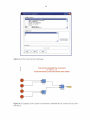
assume that the user is familiar with the basics of Matlab/Simulink. Finally, the implemented model of the coast will correspond to figure 5.1
The instructions are given on this page, and the corresponding figures on the following
ones.
1.
Start the Pandora Manager by typing pandora at the Matlab command prompt (figure 5.2).
2. Open a new Simulink model and name it coast.
3. Open the Simulink library browser.
4. Select the Pandora library.
5. Create a subsystem Inner coast and add blocks and connections according to figure
5.3.
6. Create a subsystem Outer coast and add a blocks according to figure 5.4. Note, that
you can also copy it partly from the Inner coast subsystem.
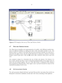
7. Connect the two subsystems according to figure 5.5 and add a Radionuclide Manager block, an Element-specific Constant+ block for inflow and a Plot block.
8. Use the Pandora Manager to set the number of inputs on the Plot block by selecting
the block either directly in the model or in the list box in the Manager, and then
pressing the Set no. of inputs button and set the number of inputs to 2.
9. Input the parameter values by pressing the Edit parameters locally button in the
Parameters tab in the Manager. Put in element-specific and site-specific parameter
values according to figures 5.6 and 5.7.
10. Select the Configuration parameters ... settings from the Simulation menu in Simulink as in figure 5.8.
11. Run the model.
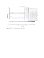
12. When simulation is ready the plot in figure 5.9 should be shown:
36
G]lu [-Xl
.I Pandora Manager : olkiluoto
File
Tools
Report
~
Help
11 Nuclides 11 Subsystems!! Functions 11 Parameters 11
Run
List:
~ Result-Report blocks
~ Plot-Manager blocks
Plot
Plot1
Plot2
Plot I View table
Set no. of inputs
Report settings
V
System settings to report
Figure 5.2. Step 1 of the implementation of the test case model.
37
~ coast/Inner coast
E)le
~dit
~iew
GJ[Q) ~
2imulation
FQ.rmat
Iools
tfelp
LeveiWaier
ltESUSP
RI! •J.SP
Setliment
I
,-----J
--tslt
Setliment
o--
'~
Msetl
TCsw
rate
TCsd
Ready
'so%
!ode15s
Figure 5.3. Step 5 of the implementation of the test case model (the Inner coast subsystem).
38
~§ ~
1::1 coast/Outer coast
Eile
Ready
~dit
~iew
2_imulation
fQ!'mat
Iools
t!elp
lode15s
Figure 5.4. Step 6 of the implementation of the test case model (the Outer coast subsystem).
39
CJ[QJC8J
~ coast
Eile
!;.dit
Y.iew
2_imulation
FQrmat
Iools
t!elp
CI·M aDtOOO
211100000
I· t29 t8700000
M•98 .WOO
hi i·ft '7MOO
hllp21'7 2t44000
PUo289 24tt0
~taB
Plcrt
PANIDORA
LeveiWater , ....
c·r....,
~___,.. ++,./
LeveiWater -o;;;;;
cant. ,,_.. 1,..,._.
._.lnftow
...... rt ,,_.. 1,..,._.
r··••w
!mu.
Outftow , ..........rt .Dat.r~
Inner co;ast
Outer coast
(so%
Ready
I
lode15s
Figure 5.5. Step 7 of the implementation of the test case model (connection of the subsystems Inner coast and Outer coast).
g
r;J[QJ ~
Parameter Editor
Element Specific Parameters
Name
Inflow - Cl-36
I
value
1.0
Inflow - Cs-135
1.0
Inflow - 1-129
1.0
Inflow - Mo-93
1.0
Inflow - Ni-59
1.0
Inflow - Np-237
Inflow- Pu-239
1.0
1.0
Kd sea - Cl-36
0.0010
Kd sea- Cs-135
10.0
Kd sea -1-129
0.3
Kd_sea- Mo-93
0.0010
Kd sea - Ni-59
10.0
Kd sea - Np-237
10.0
Kd sea - Pu-239
100.0
Apply
J
l
Parameter Type
0
Universal
0
Site Specific
Close
Figure 5. 6. Step 9, phase 1 of the implementation of the test case model (input of element-specific parameters in the Parameter Editor).
40
~ Parameter Editor
GJ[g) ~
Site Specific Parameters
Name
lnnerCoast .Depth
lnnerCoast .Msed
lnnerCoast .RESUSP
lnnerCoast .RETTIME
lnnerCoast .SR
lnnerCoast .Susp
OuterCoast .Depth
OuterCoast .Msed
OuterCoast .OUTFLOVV
OuterCoast .RESUSP
Outer Coast .RETTIME
OuterCoast .SR
Outer Coast .Susp
I
value
2.3
10.0
0 .2
45 .0
2.0
0 .0010
7 .0
10.0
44
0 .2
45 .0
0.2
0 .0010
Apply
] [
Parameter Type
0
Universal
0
Element Specific
Close
Figure 5. 7. Step 9, phase 2 of the implementation of the test case model (input of sitespecific parameters in the Parameter Editor).
[8]
~ Configuration Parameters: tensit_test_modeUConfiguration
Select:
j [ Simulation time
lTllll·~~~-·····
!····Data Import/Export
!····Optimization
$··Diagnostics
!···· Sample Time
!···· Data Integrity
!···· Conversion
!···· Connectivity
!···· Compatibility
i.... Model Referencing
!····Hardware Implementation
!···· Model Referencing
El·· Real· Time Workshop
!···· Comments
!···· Symbols
!···· Custom Code
!···· Debug
i.... lnterface
Start time:
Stop time: j1 00000
jo.o
- Solver options- - - - - - - - - - - - - - - - - - - - - - - - - - - - -1
Type:
Max step size:
Min step size:
IVariable-step
i] Solver:
Iode23s (stiff/Mod. Rosenbrock) iJ
rla-u-to- - - - - - - - Relative tolerance: j1 e-3
Iauto
Absolute tolerance: li-a-ut_o_ _ _ _ _ _ _ __
lra-ut_o____________
Initial step size:
I
Zero crossing control: Use local settings
·-·~~------------------------------~====~-----~------~---1
~
.QK
.!;;ancel
tlelp
I.
apply
Figure 5.8. Step 10 of the implementation of the test case model (simulation settings).
I
41
Coast simulation
-
-...
............
-
~
Time {year]
Figure 5.9. Plot of result from the test case model.
Inner coa st.LeveiWater/(CI-36)
Inner coast. LeveiWater/(Cs-135)
Inner coast. LeveiWater/(1-129)
Inner coast. LeveiWater/(Mo-93)
Inner coast .LeveiWater/(Ni-59)
Inner coast. LeveiWater/(Np-237)
Inner coast. LeveiWater/(Pu-239)
Outer coast. LeveiWater/(CI-36)
Outer coast. LeveiWater/(Cs-135)
Outer coast .LeveiWater/(1-129)
Outer coast. LeveiWater/(Mo-93)
Outer coast.LeveiWater/(Ni-59)
Outer coast . LeveiWater/(Np-237)
Outer coast . LeveiWater/(Pu-239)
43
6
BENCHMARKING, TESTS AND COMPARISONS
Pandora as well as its predecessor Tensit (Jones et al. 2004) has been benchmarked,
tested and compared with other similar tools. Ecolego (Avila et al. 2000), another tool
based on the Matlab/Simulink software and utilising similar model approach as Pandora, has undergone several comparisons with other tools (Maul et al. 2003). We believe that the successful results from these comparisons are implying also confidence to
Pandora.
The predecessor of Pandora, Tensit, was compared with several analytical results as
well as numerical results from other simulation tools (Robinson et al. 2003); the comparison is described in Jones et al. (2004).
For testing Pandora version 1, one of the models used in the Tensit tests (SN2, see the
references above) was implemented and run as described in section 6.1.
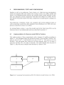
6.1
Implementation of reference model SN2 in Pandora
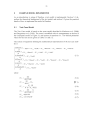
This model consists of three compartments with a transport of nuclides according to
figure 6.1. The calculation takes into account the decay of two nuclides: Nuclide 1 decays at a rate of 1x10-4 f 1 and Nuclide 2 at a rate of 1x10-2 f 1. The source to A is for
Nuclide 1 only and equals zero except for two time intervals: from 0 to 10 years (1
mol/year) and from 30 to 50 years (2 mol/year). The initial transfer rates are given in
Table 6.1. After 40 years all transfer rates decrease by a factor of 100.
H
A
~
..
c
,.
/
B
Nuclide 1
Nuclide 2
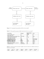
Figure 6.1. Conceptual representation of the SN2 reference model (Jones et al. 2004).
44
Table 6.1. Initial transfer rates for the SN2 reference model. After 40 years all transfer
rates decrease by a factor of 100.
From
A
B
c
To
Nuclide 1
B
0.01
................................. ................................................................................................................................................................
c
0.001
·························································································· ·························································································
A
0.1
Nuclide 2
0.001
0.1
0.1
The Pandora implementation (figure 6.2) utilises, in addition to the Pandora blocks,
Pulse blocks and Embedded Matlab function blocks from the Simulink library (for further details see the Matlab documentation). The configuration parameters are shown in
figure 6.3.
The results of the Pandora implementation are compared to the AMBER calculations
(Robinson et al. 2003) after simulation times of 10 and 100 years, as listed in Table 6-2.
The results show very good agreement.
Nuclide 1 6931.4718
Nuclide 2 69 .3147
PAN DO RA
Result Report1
~Nuclide1
Pulse 1
Filter2
~Nuclide1
Pulse 2
Embedded
Filter3
Embedded
MATLAB Function1
rate1
TCbc
C.level
L------•TCca
C.outl
rate2
Figure 6.2. The SN2 reference model implemented in Pandora.
45
(g)
[:) Configuration Parameters: SN2/Configuration
Select:
'···· Solver
!.... Data Import/Export
!. . Optimization
$-- 0 iagnostics
j.... Sample Time
j.... oata Integrity
).... Conversion
j.... Connectivity
j.... Compatibility
!.... Model Referencing
!---- Hardware Implementation
!---- Model Referencing
8-- Real-Time Workshop
!---- Comments
lj'-SL-im-u-lat-~n-t-ijm_me
Start time:
______________________________________________
Stop time: !100
~l ~
.
- Solver options- - - - - - - - - - - - - - - - - - - - - - - - - - - - - - - - - - - - - - - - - - ,
Type:
IVariable-step
I
iJ
Min step size:
Solver:
ode45 (Oormand-Prince)
r-l
au- to- - - - - - - - Relative tolerance: j1 e-7
I auto
Absolute tolerance: ,...I
au- to_ _ _ _ _ _ __
Initial step size:
lrau- to- - - - - - - - - - -
Max step size:
-
I
Zero crossing control: Use local settings
..:.1
.QK
.Cancel
!:!elp
8pply
1
Figure 6.3. Configuration parameters used in the Pandora test run.
Table 6.2. Results of the Pandora implementation and run of the SN2 reference model
compared with the results with AMBER (Robinson et al. 2003).
Results from
Results from
AMBER
Pandora
A
Nuclide 1
10
9.51191
9.511911532
A
Nuclide
2
10
0.00466821
0.004668213
·····················································································································- ···········································-······
B
Nuclide
1
10
0.481807
0.481807088 ..
......................................................... ····························································- ........................................... .......................................................
................................................ ..........................................................................................................
B
Nuclide
2
10
0.000137849
0.000137849
.......................................................................................................................-.......................................................................
.................................
C
Nuclide _1.......................................... 10
0.00128305
0.001283046
................................................
........................................
C
Nuclide 2
10
2.97307E-5
2.97308E-05
A
Nuclide 1
100
45.5501
45.55008314
............................................. .................................. ........................................................................................ ............................................ ....................................................................................... .....................................
..................................................... .
A
Nuclide 2
100
0.220230
0.220230038
....................................................................................................................................................................................................................................................................................................................................................................................................
B
Nuclide 1
100 ........................................... .........................................
4.09113
4.091136749
............................................................. ...............................................................
.......................................................................................................
.
B
Nuclide
2
100
0.0188336
0.018833612
................................................................................ ........................................................................................ ...................................... .................................................................................................................................................................................................
C
Nuclide 1
100
0.0249555
0.024955533
................................... ..................................................................................................
.....................................................................................................
... ..................................... .................................. ..
C
Nuclide 2
100
0.00142203
0.00142203
Compartment
ooo oooooooOoooooooooo ooOOOOOOOOOoOOOO
Nuclide
OOoOooooOoOooo o ooOOoOOoOOoOO .. OOoOOOOOOooOOO .. MoOO .. OOOOOOO .. O"'OO"OoO
Time [Years]
' ' ' ' ' ' ' ' ' ' ' ' ' ' ' ' ' ' ' ' ' ' ' ' ' ' ' ' ' ' ' ' ' " ' ' ' ' ' ' '' ' ' ' ' ' ' '
ooooo oo ooooooo ooooo-
o oooooo oo ooooooooo ooo ooo .. oooooooooooo oooooooooo oooooooo
ooooooooooooooo
' ' ' ' ' ' ' ' ' ' ' ' ''''''"'"ooooooooooooo .. .. o
47
ACKNOWLEDGEMENTS
The Finnish company Posiva Oy and the Swedish company SKB are acknowledged for
supporting the project, as well as for providing financial support.
Many fruitful discussions have taken place between people involved. We would especially like to mention the valuable ideas and advise from Rodolfo Avila, Ari Ikonen,
Ulrik Kautsky and Fredrik Vahlund.
49
REFERENCES
Avila, R, Broed R. & Pereira, A. 2003. Ecolego- a Toolbox for Radioecological Risk
Assessments. International Conference on the Protection of the Environment from the
Effects of Ionising Radiation, 6-10 October 2003, Stockholm, Sweden.
Bergstrom, U., Nordlinder, S. & Aggeryd, I. 1999. Models for dose assessments. SKB
TR-99-14. Svensk Karnbranslehantering AB.
Jones, J., Vahlund, F. & Kautsky, U. 2004. Tensit- a novel probabilistic simulation
tool for safety assessments Tests and verifications using biosphere models. SKB TR-0407, Svensk Karnbranslehantering AB.
Karlsson, S.,Bersgtrom, U. & Rosen, K. 2000. Sensitivity analysis for modules for
various biosphere types. SKB R-00-39. Svensk Kambranslehantering AB.
Karlsson, S. & Bersgtrom, U. 2000. Dose rate estimates for the Olkiluoto site using the
biospheric models of SR 97. Working report 2000-20. Posiva Oy.
Maul, P., Robinson, P., Avila, R., Broed, R., Pereira, A. & Xu, S. 2003. AMBER and
Ecolego Intercomparisons using Calculations from SR97. SKI 2003:28, SSI 2003:11.
SKI and SSI, Sweden.
McKay, M. D., W. J. Conover & Beckman, R. J. 1979. A Comparison of Three
Methods for Selecting Values of Input Variables in the Analysis of Output from a
Computer Code. Technometrics 21: 239-245.
Robinson, P. C., Penfold, J. S. S., Little, R. H. & Walke, R. C. 2003. AMBER 4.5
Verification: Summary. Document Reference Number: QRS-1 059B-1. Available
August 18th 2003, http://www.enviros.com/PDF/Services!Users&References_v102e
.pdf
SKB 2004. Interim main report of the safety assessment SR-Can. SKB TR-04-11.
Svensk Karnbranslehantering AB.
Vieno, T. & Ikonen, A. T. K. 2005. Plan for safety case of spent fuel repository at
Olkiluoto. POSIV A-2005-0 1. Posiva Oy.
51
APPENDIX A: INSTALLATION OF PANDORA
A.1 Software requirements
Pandora was developed on Matlab7.0.1©, Simulink 6.1©, Windows NT/XP© and Microsoft Excel 97©.
For correct operation of Pandora it is advisable to use these software releases or later
ones.
A.2 Installation of Pandora version 1
The Pandora version 1 is delivered in a compressed file Pandora.zip. To install the
package
1. Unpack the file Pandora.zip. When the file is unpacked a directory called
Pandora is created.
2. Add the path (with subfolders) to this directory e.g. C:\Pandora to the Matlab path. This is done from the File > Set Path menu in Matlab.
3. You should now be able to see the Pandora library in the Simulink library
browser as in Figure A.l.
l;Jiu ~
~ Simulink Library Browser
Eile
!;dit
~Jew
t:!.elp
Plot: Export numerical data to matlab graph.
Simulink
Pandora v1.04
Mole2Bq
.,..~~~~
....- - -
Real-Time Workshop
Parameter Report
Simulink Extras
Stateflow
Plot
/
rate
..
1
I'
Ready
Figure A.l. Pandora in the Simulink library browser.
I
Reservoir