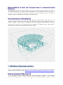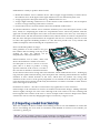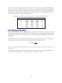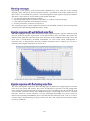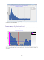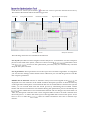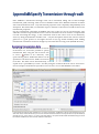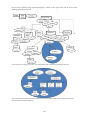
1
Room Acoustics Software ODEON User’s Manual Z X O Y ODEON Room Acoustics Software Version 13 Full User’s Manual Written by Claus Lynge Christensen and George Koutsouris Published in 2015 Odeon A/S Scion DTU Diplomvej, bulding 381 DK-2800 Kgs. Lyngby Denmark Tel: +45 8870 8845 Fax: +45 8870 8090 www.odeon.dk Thank you for using ODEON, the Room Acoustic Software package that helps you make complete studies of room acoustics for any space through simulations and measurements! We hope you will enjoy working with ODEON and that you will find it extremely useful in the acoustical design of new spaces and improvement of existing ones. ODEON has a very user-friendly interface that allows setting up a project very fast and elegant presentation of results. This manual is intended to serve as an introduction on modelling room geometries in ODEON software, on the facilities for measurement and simulations and the applied calculation principles behind. It will not cover in depth all facilities included in the ODEON software; explanations of displays, calculation parameters, results, etc. are available as context sensitive help from within the ODEON applications (shortcut F1). It is recommended to use the online help to learn about the specific features available from the different displays, the interpretation of results, calculation parameters, etc. The contents of this manual are as follows: Chapter 1 covers installation of the program, changes from previous versions etc. Chapter 2 covers geometry modelling. New releases of ODEON often include new facilities which can speed up the modelling process as well as tools for verification of geometries. Some of the facilities are; a plug-in for Google Sketchup, extensive support for import of CAD models in the .dxf as well as the .3ds (3D Studio) format and a stand-alone drawing program for modelling of so called extrusion models. Tools for verification of room models are also covered in this chapter. With improved support for 3rd party tools for geometry modelling, knowledge about ODEON parametric modelling language is becoming of less importance. The advanced user will find that the description of the .par format has been moved to appendix E. The format features support for symmetric and semi-symmetric rooms, use of constants, variables, counters, loops etc. and can be useful when studying geometrical parameters such as angle of reflectors etc. As all geometry, also imported ones, are stored in the .par format, it is possible to add features described in terms of parameters to an imported geometry if familiar with this format. Chapter 3 deals with the materials to assign to the surfaces of the rooms; absorption, scattering and transparency coefficients as well as transmission data. Special materials that may speed up the modelling process and how to manage the material library are also covered in this chapter. Chapter 4 deals with the auralisation options in ODEON Auditorium and Combined; the hardware requirements, how to publish calculated sound examples on the Internet or on audio CD's etc. Chapter 5 introduces the calculation principles used in ODEON, giving an idea on the capabilities and limitations the simulation part of the program. Chapter 6 describes important calculated room acoustic parameters available in ODEON, how they are calculated and how to interpret the results. 1 Chapter 7 describes the various calculation parameters available in the program. Most of the parameters are automatically set to reasonable values by ODEON; however for special cases you may need to adjust some of the calculation parameters. Chapter 8 is the discussion on quality of results and how to achieve good results. This chapter may be relevant once familiar with the program. Chapter 9 describes how to extend the library of directivity patterns available for point sources and the use of directivity patterns in the Common Loudspeaker Format, CLF. Chapter 10 introduces the line array sources discussing some basic principles behind array source design. Chapter 11 presents the integrated impulse response measuring system in ODEON. The chapter explains which measuring methods are used, how to obtain a healthy impulse response and how to obtain room acoustic parameters as the results. The chapter ends with an annex giving examples of good and bad impulse responses. Chapter 12 is describes how to use ODEON’s Genetic Material Optimizer for calibrating a room model towards a real room. The Genetic Material Optimizer makes use of genetic algorithms in order find the list of materials (absorption coefficients) that lead several simulated parameters to match with measured ones. 2 This legal document constitutes the complete agreement between you, the end user (either an individual or a single entity) and Odeon A/S. All rights not expressly granted in this License Agreement are reserved by Odeon A/S. The right to use the Odeon software is sold only on the condition that the user agrees to the following License Agreement. The Odeon software, auxiliary applications, and documentation are owned by Odeon A/S and are protected by copyright laws and international copyright treaties, as well as other intellectual property laws and treaties. The SOFTWARE PRODUCT is licensed, not sold. You shall be held legally responsible for any copyright infringement that is caused or encouraged by your failure to abide by the terms of this Agreement. Odeon A/S retains sole title and ownership of the ODEON software, regardless of the form or media in or on which the original and other copies may exist. As the licensee, you own the magnetic or other physical media on which the ODEON program is subsequently recorded or fixed. This Agreement is not a sale of the original ODEON software or any copy thereof. All rights are reserved by Odeon A/S. In consideration of payment of the License fee, Odeon A/S grants each customer (a private person or a company registered in a country) a non exclusive right to use the ODEON software. This Agreement grants you the right to make copies of the software for archival purposes, and to copy the software on the hard disk of your computer. The software may be loaded onto multiple computers, but can only be fully operational on a single computer at any given time. The computer operating the ODOEN software needs to have the hardware key delivered with the software attached to the USB port. Granting of a license is bound to ODEON software use with a hardware key. The hardware key holds the license information and determines the version and edition of the Odeon software that can run when the hardware key is attached to the computer. If a hardware key is defective during the warranty period (first licensed year), Odeon A/S will replace the hardware key. The customer will pay the hardware key fee for replacing the hardware key should it become defective after the warranty period. The hardware key contains the name and country of the licensee which are displayed in the software, on print outs from the software and on graphics exchanged from the software. 3 The modification, adaptation, translation, reverse engineering, de-compiling, disassembling, attempt to discover the source code of the software, or the creation of derivative work based on ODEON software is strictly prohibited. In no way may you transfer, assign, rent sublicenses, lease, sell, or otherwise dispose of any portion of the software on a temporary or permanent basis. The ODEON software is licensed only to the licensee. In no way may you transfer, assign, rent sublicenses, lease, sell, or otherwise transfer any portion of the license on a temporary or permanent basis (this includes transfer between branches of international companies that are registered in different countries). The license may only be transferred to anyone with the prior written consent of ODEON A/S. Any authorized transfer of the ODEON software shall be bound by the terms and conditions of this Agreement. This license is effective until termination. This license will terminate automatically without notice from ODEON A/S if you fail to comply with any provision of this Agreement. Upon termination, you shall destroy the written materials and all copies of the ODEON software, including archival copies, if any. Neither Odeon A/S nor anyone else who has been involved in the creation, production, distribution or delivery of this program shall be liable (including, without limitation, damages for loss of profits, business interruption, loss of information, incorrect results, recovery of data, or other pecuniary loss) for any direct, indirect, consequential, or incidental damages resulting from any defect in the software, update version, or its documentation, or arising out of the use, the results of use, or inability to use the product, even if ODEON has been advised of the possibility of such damage or claim. ODEON A/S make no warranty or representation, either expressed or implied, including, but not limited to, implied warranties or merchantability and fitness for a particular purpose, with respect to this product, As a result, this software is sold "as is" and you the licensee are assuming the entire risk as to its quality and performance. No ODEON A/S Distributor, agent, or employee is authorized to make any modification, extension or addition that will increase the scope of this warranty. ODEON A/S may create, from time to time, update versions of the ODEON software. Odeon A/S reserves the right to make changes to the software or its documentation without notice. Major updates e.g. from Odeon 11 to Odeon 12 will be made available to registered users who have a valid Maintenance and Support Agreement or who purchase an upgrade. Minor service updates e.g. from v 12.0 to 12.01 or 12.1 may be made available for download and may also be used by the licensee without a valid Maintenance and Support Agreement if the hardware key permits running the update. 4 The Odeon Auditorium and Combined (excluding the demo version) installs with a number of anechoic recordings that may be used with the Odeon software without restrictions, except for the orchestra recordings. For the orchestra recordings in the WaveSignals\Orchestra folder special restrictions apply: Customer acknowledges that the anechoic recordings are the sole property of TKK, Helsinki University of Technology. Customer acknowledges the right to use the recordings for internal use only and the right to make one copy for archival and backup purposes. Customer agrees not to modify or remove, and not to tamper with or disable any automated display, performance, or execution of, any credits, references or notices, without the prior written consent of TKK, Helsinki University of Technology. Customer agrees not to copy, modify, adapt, combine, publish, rent, lease, sell, distribute the recordings or sublicense or otherwise transfer the sublicense. If the anechoic recordings are used in the Customer's work in such a way that an ordinary, reasonable user familiar with the recordings would be likely to recognize it, Customer agrees to include the following notice in the resulting work: "Derived from anechoic symphony orchestra recordings by Jukka Pätynen and Tapio Lokki, Helsinki University of Technology and licensed from Odeon A/S". This Agreement constitutes the entire agreement between you and Odeon A/S concerning the ODEON product. If any provision of this Agreement shall be declared void or unenforceable, the validity of this Agreement and all other provision shall not be affected. ODEON product support and service is only provided to registered ODEON users with a valid support agreement. 5 1.1 1.2 1.3 1.4 1.5 ................................................................................................................. 8 Installing and running the program .........................................................................................8 Upgrading from previous versions ........................................................................................... 8 What’s new in ODEON 13 .........................................................................................................9 Features of previous versions .................................................................................................. 15 How to upgrade or update your current license................................................................... 17 2.1 2.2 2.3 2.4 2.5 2.6 2.7 ...................................................................................................................... 20 Pre-calculated Rooms................................................................................................................ 21 Guidelines on room modelling ................................................................................................ 23 Importing a model from SketchUp ......................................................................................... 25 Importing DXF and 3DS files ................................................................................................... 27 The ODEON Extrusion Modeller ............................................................................................ 33 Model check in ODEON ........................................................................................................... 39 Combining geometries .............................................................................................................. 41 3.1 3.2 3.3 3.4 .......................................................................................................... 43 Generic point sources................................................................................................................ 43 Natural point sources................................................................................................................ 43 Common loudspeaker format, CF1 and CF2 files ................................................................. 44 Creating new directivity patterns in the ODEON .So8 format ........................................... 45 4.1 4.2 4.3 4.4 .......................................................................................................................................... 49 Material Library (Right side of Material List window) ........................................................ 49 Surface List (Left side of Material List window) ................................................................... 51 Manage material library and material list.............................................................................. 53 Opening an existing room form a version earlier than version 10 for the first time ........ 54 ................................................................................................................................... 55 5.1 5.2 Listening to Binaural Room Impulse Responses............................................................ 55 Making offline auralisations – creating WAV files ............................................................... 62 6.1 6.2 ............................................................................................................ 65 What can we model in ODEON .............................................................................................. 65 Global decay methods .............................................................................................................. 66 6.3 6.4 6.5 6.6 6.7 6.8 6.9 6.10 Quick Estimate .................................................................................................................... 66 Calculation of Response from Sources to Receivers ............................................................. 67 The Reflection Based Scattering coefficient ........................................................................... 72 Oblique Lambert ........................................................................................................................ 77 Diffraction over screens and round objects (Screen diffraction) ......................................... 78 Radiated rays from a source .................................................................................................... 79 Processing reflection data for auralisation in Single Point Response ................................. 80 Calculation method for Reflector Coverage .......................................................................... 81 ............................................................... 82 ............................. 88 9.1 ........................................................................................................ 92 Sources of error .......................................................................................................................... 93 10.1 10.2 .................................................................................................................... 97 Stacking the units ...................................................................................................................... 97 Playing with delay ..................................................................................................................... 99 6 10.3 10.4 10.5 10.6 Playing with level .................................................................................................................... 101 Combining delay and level adjustments .............................................................................. 102 Using the equalizer.................................................................................................................. 103 Bringing the array into the room ........................................................................................... 103 11.1 11.2 11.3 11.4 11.5 11.6 11.7 .......................................................................................................... 104 Technical Background............................................................................................................. 104 Equipment ................................................................................................................................ 106 Measurements and Processing .............................................................................................. 106 Measurement set-up................................................................................................................ 111 Editing Impulse Responses .................................................................................................... 113 Making auralisations with Impulse Responses ................................................................... 114 Examples of Impulse Responses - Warnings ....................................................................... 115 12.1 12.2 12.3 ............................................................................................ 125 General Steps for Material Calibration ................................................................................. 125 How Genetic Algorithms Work............................................................................................. 128 Perform a Material Optimization .......................................................................................... 131 ............................................................................................................................................ 138 Appendix A: Vocabulary............................................................................................................................ 141 Appendix B: Specify Transmission through walls.................................................................................. 143 Appendix C: Description of XML format for import of array loudspeaker data ............................... 146 Appendix D: Modelling rooms in the ODEON Editor........................................................................... 156 Appendix E: Mathematical expressions ................................................................................................... 188 Appendix F: Importing geometries-compatibility .................................................................................. 189 7 To run ODEON, your PC must be running one of the operating systems supported by ODEON: 32 bit/64 bit Windows Vista, 32 bit/64 bit Windows 7, 32 bit/64 bit Windows 8. ODEON comes on a USB drive containing the edition of ODEON purchased (Basics, Industrial, Auditorium or Combined). As an alternative you may download the most resent updated version including service updates that has been made since the production of the USB, from www.odeon.dk/updates. To install the program: a) Double-click on the file with the name of the edition you wish to install, e.g. InstallOdeon12Combined.exe to install the program. b) To run the program, the supplied hardware key (Rockey 6 Smart – R6 Smart) must be inserted into the USB port on the PC. If you start the program without the hardware key it can only be used in viewer mode. c) When you have installed the ODEON software please check for the most resent updates at www.odeon.dk/updates. If you are upgrading from previous versions of ODEON, read on to learn about the changes in ODEON. Below is a list of issues which you should be aware of when upgrading from previous versions. ODEON version 13 runs on Windows 8 (32/64 bit editions), Windows 7 (32/64 bit editions) and Windows Vista (32/64 bit editions). ODEON 13 is a major upgrade, please see section 1.3. Though ODEON 13 is capable of loading and converting older projects into the version 13 format (forward compatibility) an older version of ODEON may not load a room once it has been loaded into ODEON 13. ODEON 13 includes a large number of enhancements – for a fairly complete list see section 1.3 or open the help file from within the ODEON software (press F1 from within ODEON, then click Whats new in ODEON 13 entry in the Contents menu). When upgrading from versions earlier than version 8, it is essential to learn about the new methods for handling of scattering. Chapter 4 covers the material properties to assign to surfaces; chapter 6 covers the calculation principles including handling of scattering and chapter 8 covers the choice of calculation parameters. 8 If performing a major upgrade, typically a full version number or more e.g. from version 8 to version 9 then ODEON will install to a new directory for that version without changing the existing installation. If you have no wishes to use the old version of ODEON then it is recommended to uninstall the version(s) using the Windows Start|Control panel|Add /remove programs feature. Remember: If keeping an earlier version, be careful not to mix the use of old and new versions – although we do strive to maintain forward compatibility we cannot guarantee that a room which has been loaded into a new version of ODEON will also load into an older version without problems. If you upgrade from a version earlier than 6 then we do recommend that you read carefully through the manual as if you were a newcomer to ODEON. There are a substantial differences between the early versions of ODEON and the ODEON software as it is today – modelling has been made easier, calculation principles has been enhanced and a huge amount of new features has been added. The only project file from versions earlier than 3.0, being fully compatible is the surface file (.sur). The rest of the project files are no longer valid. And even though the .sur format is still valid, it is not recommended to model rooms in this format. The .par format is a much more efficient format. If you are having problems loading a room, which was created and worked fine in one of the above listed versions of ODEON, this is probably due to a change that has been made to the surface numbering mechanism applied in ODEON. The numbering mechanism has been changed slightly in order to avoid a conflict, which appeared when using ‘symmetric surfaces’ along with modelling entities such as CountSurf, Box, Cylinder etc. and in particular to make the automatic surface numbering work without any problems (when the NumbOffSet is set to Auto). If having problems loading a room due to the reasons just mentioned, ODEON will either give an error message that surfaces are repeated in the geometry file or that materials are not applied to all surfaces. In these cases you may wish that ODEON use the old numbering mechanism – this can be done using the Version4 .par file; As the first line in the geometry file, just after the ### sign, type: flag in the Version4 TRUE Once the old incompatible code ends, Version4 may be set to FALSE again. The new version of ODEON is packed with a bundle of attractive features and enhancements: All lists and input fields have been freshened up in ODEON 13: Materials list, source-receiver list, job list etc. they all have been equipped with shorting functions, better display colors and easier editing properties, such as multi-delete, copy-paste etc. 9 In ODEON 13 it is possible to change source or receiver position directly on the 3D Edit Source display using CTRL+LMB. While you rotate the geometry a grid is adjusted to the visible plane to help anchoring the source on its nodes. In the next figure the grid is displayed for the XZ plane. Making an array of sources of receivers is easier than ever! Now all members of the array are displayed in the 3D view in real time before changes are confirmed. 10 The already known directivity polar plot editor in ODEON has now been re-built offering easier construction of directivity balloons. Attractive visualization features have been added in the reflector coverage display. Rays from source/receiver to reflectors/audience can be displayed with varying density and colors according to layers. 11 Often acoustic refurbishment is needed in an existing room that suffers from bad acoustics. The room acoustician is asked to make a virtual model of the existing room. Materials are not perfectly known for all surfaces, so calibration or fine-tuning is needed in order to match simulations with measurements. ODEON 13 has been equipped with an optimization tool based on genetic algorithms. An initial estimate of materials is required. Then the algorithm searches for the best set of absorption coefficients, by a genetic evolution process, that makes simulations match with measurements. A tool for investigating how the number of rays and the transition order affect the agreement between simulations and measurements. The tool calculates the average error in JND as a function of the number of rays. Different curves are displayed for different transmission orders, helping the user to determine the optimal number of rays and transmission order for the simulations. 12 This tool removes the requirement of fixed conditions in the measuring chain, which is common rule in ordinary calibration procedures, such as diffuse field calibration and free field calibration. The two-step sound source calibration adds a second step to the normal reverberation room or free field calibration methods, in order to allow compensation for any shift in the broadband gain, from the calibration to the field measurement condition. Enhanced Bass response is audible in the auralisation algorithms of ODEON 13. The bank of octave band filters has been extended towards 16 Hz which provides a better low frequency auralisation. Record an impulse response in an existing room. Go home and try how different signals would sound inside the room. Speech, music, noise, anything now can be convolved and auralised exactly as it is done so far in simulations. 13 A recorded impulse response can be further edited in the ODEON measuring system. An FFT frequency response is available now, as well as phase and cepstrum plots (spectrum of the frequency response). 14 Although ODEON offers superb automatic truncation of recorded impulse responses at the noise floor and the onset time, a group of manual operations are now possible for those who wish to have full control on the impulse response file. Together with the existing crop function, editing an impulse response file becomes an extremely time efficient task. Very often a room model needs to have several openings in the geometry: open windows, open ceiling etc. Moreover there are projects that deal with pure outdoor sound propagation, such as an atrium courtyard, a street canyon etc. In all these cases a bounding box needs to be constructed by the user. Now an easy to use command has been added in the ODEON editor, which builds a bounding box to automatically include the whole geometry. Below we have gathered the most important developments introduced with the recent ODEON versions. Please read more online at http://www.odeon.dk/development-room-acoustics-software. A very important version, brought simulations and measurements together. A room impulse response measuring system was introduced that allows capturing of impulse responses with the 15 aid of a loudspeaker, a microphone and a laptop. The tool is available in all editions (from Basics to Combined) and practically offers simulations and measurements inside the same software package. Moreover, ODEON 12 was equipped with full support for ISO 3382-3 - Open Plan Offices, tools for grouping receivers in the multi-point response, two types of radiation in line and surface sources, calculation of IACC and many more enhancements. Read more about them online at http://www.odeon.dk/odeon12features. Parallel processing was introduced with ODEON 11, providing faster calculations on multicore computers. The parallel processing is used for multi-point and grid responses, where many receivers have to be calculated at a time. In addition, a Fibonacci Spiral distribution used in ray tracing, allows a perfect distribution of source radiation pattern. A Room acoustic parameter list interface allows the user to edit existing parameters and create his/her own ones. This is a great feature for improving parameters of inventing new ones, especially for research purposes. Apart from these, an improved calculation setup, improved grid scaling, echo detection curves, dynamic diffusion curves and many other features were introduced. You can read more online at http://www.odeon.dk/version-11. ODEON 10 is Unicode (and utf-8) enabled allowing text in complex character sets to be saved with your projects, whether this is in the text files such as the geometry files (.par) or texts composed in the various comment fields in ODEON (the material library is not fully Unicode enabled yet). In particular Unicode allows text in Asian character sets (Japanese, Chinese and Korean) to be saved from within the ODEON application. It is also possible to save text which is a mix of texts in different character sets. When upgrading to version 10 or later, the order of materials in the Material list has been revised – please see Chapter 4. Read more on the features introduced with version 10 at http://www.odeon.dk/version-10. With ODEON 9.1 is delivered a new type of Dongle, which makes it easier for the user to install new upgrades. This is more thoroughly described below in chapter 1.4 and at www.odeon.dk/dongle-update. Version 9.1 has a far better auralisation option than previous versions for presentation through 2 loudspeakers, called Super stereo. With Super stereo you can make 2 loudspeakers have a much more spacious sound with the right frequency response for this type of auralisation. In Chapter 2 an intro on how to do this can be found. As an example of use; if you are both musician and acoustician, you can make an auralisation of a recording of your own music played in a room you have modelled in ODEON so it sounds right, on your own loudspeakers. Some outdated directivity files such as TlkNorm.so8 have been replaced by TlkNorm_Natural.so8 which is smarter for auralisation use, where there might be a risk of adding the overall frequency response twice to auralisation output; once from the directivity pattern and once more from the auralisation signal which inherently includes the same source spectrum (please see chapter 5 for further information). With the _Natural version of the directivity files it is possible to obtain correct equalization of auralisation output while also achieving correct prediction of SPL. Therefore the _Natural versions of the directivity files should be used when defining new sources. The old versions of the files are kept in \old_so8\ a subdirectory to the \Dirfiles\ directory. If you wish to use the old directivities in old/existing projects, then open the Source receiver list and click the Repair broken directivity links button (shortcut Ctrl+L). See Chapter 10 for more information about sources and directivities. 16 For ODEON 9.1 and later versions, your ODEON software license is stored in a Smart Card based hardware key, the Rockey 6 Smart dongle. As an ODEON user you can have 4 ways of updating or upgrading the program after the installation of ODEON 9.1: Version number can be updated free of charge in-between the full www.odeon.dk. E.g. from version 9.1 to version 9.2 Your version can be updated to a full version number (E.g. version 10) by remote licence update. For time limited licenses, time limitations can be removed or the Run available) can be updated, by requesting a remote licence update. The Edition can be upgraded to Combined if the current edition is Basics, Auditorium, by requesting a remote licence upgrade. versions at requesting a time (hours Industrial or Your wishes for update or upgrade could be a combination of the above 4 points, which can be fulfilled by generating a remote request file and following the steps described below. 1. 2. 3. 4. Generate a license request file and send it to [email protected]. You will receive a mail with the license file, when your update or upgrade has been generated. Download the received license file to your dongle. Update your ODEON software installation as needed from the www.odeon.dk homepage. For more info on dongle update, please visit www.odeon.dk/dongle-update. A remote request file has the extension .req. To generate a Remote request file follow these steps: 1. Attach your ODEON dongle to the USB port on the PC. 2. Run the ODEON program. 3. Check what your current license includes using the Tools|License information menu entry. 4. Generate your license request file using the Tools|Generate Remote Update Request file menu entry - this will display the shown dialog. 5. Email the generated request file (e.g. User2005_Dongle102009.req) to [email protected]. 17 Once Odeon A/S has received your request file, an invoice will be processed and sent to you. When the invoice has been paid, an encrypted license file will be e-mailed to you, and this file has to be downloaded into your dongle for a license upgrade (see below). 1. 2. 3. 4. 5. Extract the license update file from e-mail to your hard disk e.g. to your desktop. Attach your ODEON dongle to the USB port on the PC. Run the ODEON program. Use the Tools|Download license update to dongle menu entry. Select the file using the Select license update file (.cif) dialog User2005_Dongle102009_ODEON Industrial_V5__Restricted_0h.cif). (e.g. select When the license has been downloaded to your dongle, you can find and install the new version or edition from the webpage www.odeon.dk/updates. You may choose to uninstall the previous version before installation. We recommend that you keep a safety copy of the installation file, e.g. if you at some point want to reinstall the downloaded version. The window below shows all the update options that may be available - whether all these options will be displayed (available) depends on the license currently stored in your dongle. Update option Update to most recent version of ODEON When a license of ODEON has been purchased for one version of ODEON it is valid for the full version number. If the license was purchased for ODEON 9.1, then license stored in the dongle will be valid for version 9.x (e.g. 9.1, 9.2, 9.21 or whichever versions are released before the next full release number – e.g. ODEON 11.22). The software for updating versions in between the full version numbers can be obtained free of charge from www.odeon.dk. Update user name (must be For copy protection your user name and country is supplied separately) embedded in the dongle. If you should wish to, you can change your user name by checking the box: Update user name, the user name can only be updated separately from the other updates. When you send the request file to [email protected] you should write the user name you wish in the email. Requested upgrade – relevant if edition is Basics, Industrial or Auditorium Default setting is “None”. In case your current edition of ODEON is ODEON Basics it is possible to request ODEON Industrial, ODEON Auditorium or ODEON Combined. In case your current edition is ODEON Industrial or ODEON Auditorium, it is possible to request ODEON Combined. It is not possible to upgrade from ODEON Industrial to ODEON Auditorium. Time license - relevant if the current version is time limited No update to time license This is the default setting. Update time limitation If current license is time limited then it is possible to update the time license i.e. to request additional run time by entering 18 Remove time limitation the desired number of hour in the box on the right. Common case for a time limited license is when you purchase a full license that it is always fed with a few hours for a start until delivery of dongle and complete payment is fulfilled. When payment has been executed we automatically send you an update file that removes time limitation. If however a few extra hours are needed before payment is completed you can request extra time with this procedure. If the current license is time limited, it is possible to request the time limitation to be removed 19 Creating new room models is probably the most time consuming task in room acoustical modelling. However, good modelling practice will greatly reduce the time used for modelling and re-modelling rooms. In order to study a room in ODEON, a file containing the room's geometry needs to be created. This file has to be imported by one of the ways described below. ODEON then creates a group of subsequent room files, calculation files and result files. All files share the same name - the name of the room - with a different extension added. Three main categories of files are used: Room files, which contain all data entered by the user. From these files both calculation and result files may be recalculated. Some of the most important extensions are .par, that describes the whole geometry, .PcS that lists the sources, .PcR that lists the receivers and .Mat that includes the materials used in the model. Calculation files, which holds data that are being reused during calculations to speed up calculation (of point response calculations). These files can be erased once job calculations have been carried out, however if they are present, future calculations are speeded up. Result files, containing all results. For example, the extension .GXX refers to the results in a grid response. See the full list of files in the ODEON help by searching for File management. Remember: Pressing the F1 key reveals the ODEON help menu with a topic associated with the window that is open. The file containing the room model must be written as an ASCII text file, having the file extension .Par (the ‘old' ODEON .Sur file format is also allowed though not described in this manual). You can choose to create the geometry file either by typing the model data directly into a text file in the supplied text editor ODEON text Editor, using the format described in Appendix D, using SketchUp, the ODEON Extrusion Modeler described in section 3.2 or a third party CAD program (e.g. IntelliCAD, Autodesk Revit, AutoCAD, 3DStudioMax, MicroStation or Rhino) which is capable of creating 3D surface models and exporting these as .dxf files as described in section 2.4. Finally you may combine the different modelling methods; import a CAD model from a CAD program and extend or correct it using tools which come with ODEON. Appendix F gives an overview of which file formats can be used with ODEON. Remember: No matter which approach you choose for modelling, always check the validity of the models. The room model must form a (almost) closed enclosure. It should also be (almost) free from warped (twisted), duplicate or overlapping surfaces. ODEON has several tools for checking models for such problems. The tools are presented in section 2.6. It is suggested that you always use these tools when working on models of some complexity. 20 Before making any models to be used in ODEON it is good idea to have a look at the pre-calculated rooms in your ODEON installation. You will see how a typical acoustic model looks – which in principle differs substantially from an architectural model, where all details mater for a visual impact. In an acoustic model only the most important details should be kept. In paragraph What to model in section 2.2 you can read more about the basic rules you have to follow. Tip: Find the pre-stored rooms in the Rooms folder in your ODEON installation. The usual path is C:\Odeon13Edition\Rooms, where Edition stands for Basics, Industrial, Auditorium or Combined. You can see all relevant paths used by your ODEON installation by choosing Options>Program setup. In the rooms folder you will find pre-calculated results in Elmia RoundRobin2 detailed.par and PTB_Studio open curtains detailed model.par which were the rooms used as test objects in the 2 nd and 3rd Round Robins (Bork, 2000; Bork, 2005). Geometry, absorption data, source and receiver positions as well as the measured room acoustical parameters are those supplied to all participants in the Round Robins, by the PTB in Germany. To compare results calculated by ODEON with those measured in the real rooms: Open the room in question. Open the JobList – the (Shift+Ctrl+J shortcut). Select one of the pre-calculated Multi point response jobs (job one or two) in the it (Alt+M shortcut). Select the Measured versus simulated tab-sheet in the Multi Point display. P1 2 P1 3 and open 3 1 2 1 4 P2 P2 Joblist 5 6 Odeon©1985-2005 Odeon©1985-2005 Hagia Irene.par is a model of a Byzantine church in Istanbul which, like the examples above, also includes measured room acoustical parameters. The church was modelled as part of the CAHRISMA project (Conservation of the Acoustical Heritage by the Revival and Identification of the Sinan's Mosques Acoustics). Hagia Irene has an approximate volume of 39.000 m3 and RT of 4,3 sec at 1000 Hz. You can find similar rooms in 21 8 9 10 11 7 3 4 Odeon©1985-2005 1 P1 2 5 6 the CAHRISMA project subfolder. These rooms need to be calculated. Open any of the rooms, access the Joblist and press ALT+A to run all jobs. Open the Jerash_Present_Empty.par ancient theatre and observe the bounding box around the room. The bounding box is not part of the actual geometry but it is necessary in such a case where the room is not watertight by itself (there is an open ceiling). The box encloses the geometry and allows ODEON to perform calculations. All sides of this dummy box are assigned 100% absorption in order to successfully model the open air. You can find more models from ancient theatres in the ERATO project subfolder. Z X O Y Odeon©1985-2013 Licensed to: Odeon Restricted version - research and teaching only! The example Studstrup Power Plant.par, found in the main Rooms folder is a model of a 11 22 20 turbine hall at a power plant. Measured 12 19 S31 S32 S34 S35 S37 S38 S40 S26 18 S29 P23 S33 S36 P42 13 S27 S25 P41 P22 S30 21 S39 S28 15 S24 14 SPL(A) is included in that example. Apart 17 23 16 Odeon©1985-2007 24 from the common point sources, surface sources have been used as well that can model the radiation of sound from an entire surface. This is due to the assumption that an engine consists of a group of surfaces that radiate sound as they vibrate. The example Transmission rooms.par, found also in the main Rooms folder includes some walls with transmission properties and it serves as a good demonstration of insulation between rooms. You can read more about transmission modelling with ODEON in Appendix B. 10 8 7 S10 S11S13 S14S16 S17 S20 6 S8S6 S4 S3 P2 P1 P21 P19 P44 S9 S12S15 1 5S18 S7 3 9 2 4 Z O X Y Odeon©1985-2013 Licensed to: Odeon Restricted version - research and teaching only! SPL (dB) at 4000 Hz >= 81.5 79.5 78.0 76.5 75.0 73.5 72.0 70.5 69.0 67.5 66.0 M6,8 64.5 P12 M6,10 M6,11 M6,9 M6,12 63.0 P13 P14 61.5 P8 P9 60.0 P10 P11 M3,137 M3,141 M3,138 M5,142M3,140 M5,143 M5,144 M3,139 M5,146 M5,145 58.5 P23 57.0 55.5 P24 P15 54.0 P17 P19 P18 P21 P22 52.5 P16 51.0 P20 M1,335 M1,334 49.5 M1,336 M1,338 48.0 M1,337 46.5 45.0 43.5 42.0 40.5 39.0 37.5 36.0 34.5 33.0 <= 32.5 Odeon©1985-2014 Licensed to: Odeon Restricted version - research and teaching only! 22 The room Oil rig.par is an example of an offshore oil platform where loudspeakers have been installed as part of an alarm system. Noisy sources have been taken into considerations and they are modelled as surface sources. This room has also been abalysed in the application note Calculation of Speech Transmission Index in Rooms which can be downloaded from the application notes page http://www.odeon.dk/applicationnotes . Tip: Some of these rooms have been set up for very accurate calculations that can take longer time. If you wish to carry out faster calculations, you may enter the Room setup and select the Engineering setting. This will provide results approximately 2 times faster without much loss in quality in results. t16 t15 t14 t13 t12 t11 t10 t9 t8 t7 t6 t5 t4 t16 t3 t2 t1 t15 t14 t13 t12 t11 t10 t9 A22 t8 t7 t6 t5 t4 t3 t2 t1 2 t16 t15 t14 t32 t31 t30 t13 A14 t12 t11 t10 t29 t28 t27 t9 t8 t7 t6 t26 t5 t4 t3 t25 t24 t16 t2 t23 t1 t22 t21 t20 t15 t14 t16 3 t15 t14 t19 t18 t17 t16 t13 t12 t15 t14 t13 t12 t16 t15 t14 t11 t10 t9 t13 t12 t11 A19 t11 t10 t9 t8 t7 t6 7 t10 t9 t8 t8 t7 t6 t5 t12 t13 t11 t5 t4 t3 t2 t7 t6 t5 t4 t4 t3 t2 t1 t10 A13 t9 t8 t1 t3 t2 t1 A7 A6 t7 t6 t5 t16 t15 t4 t3 t2 t1 t14 t16 t15 t14 A10 t13 t12 t11 t13 t10 t9 t12 t11 A16 t8 t7 t6 t10 t9 t8 t7 P3 1 t5 t4 t3 t2 t6 t5 t4 t1 t3 t2 t1 t16 t15 t14 A9 t13 A18 t12 t11 t10 t9 t8 4 t7 t6 t5 t4 t3 t2 t1 8 12 A15 t16 t16 t32 t15 t14 t15 t14 9 t31 t30 t13 t13 t12 t11 t12 t11 t29 t28 t10 t9 t8 t10 t9 t8 13 t27 t7 t6 t5 t7 t6 t5 t26 t25 t24 t4 t3 t2 t1 t4 t3 t2 t23 t22 t21 t1 t20 t19 t18 t17 t16 14 A17 A8 t15 t14 t13 t12 t11 t10 t9 t8 t7 t6 t5 t4 t3 A5 t2 t1 t16 t15 t14 t13 t12 t11 t10 t9 t8 t7 t6 t5 t4 t3 t2 t1 10 A23 15 t16 t15 t14 t13 t12 t11 t10 t9 t8 t7 t6 t5 t4 t3 t2 t1 A20 t15 t16 t14 t13 t12 t11 t10 t9 t8 t7 t6 t5 t4 t3 t2 t1 A11 16 Odeon©1985-2011 Licensed to: Odeon A/S 5 t16 t15 t14 t13 t12 t11 t10 t9 t8 t7 t6 t5 t2 t1 t4 t3 A21 t14 t16 t15 t13 t12 t11 t10 t9 t8 t7 t6 t5 t4 t3 t2 t1 A12 11 6 The model Copenhagen Central Station Array.par is available in the Auditorium and Combined editions of ODEON. This example demonstrates a PA system, installed by Duran Audio, which utilizes 20 beam steered line arrays. Several measured parameters are available including STI. Whether you choose to import your rooms from SkecthUp, by using a CAD program, by typing your rooms directly into a text file or by using the ODEON Extrusion Modeller, there are considerations that are common to either case. Some guidelines of general nature are given below. To make it as easy as possible to operate ODEON, the following orientation of room geometries should be applied (using a concert hall as the example): Z O X Y X-axis pointing towards the audience Y-axis pointing to the right as seen from the audience Z-axis pointing upwards An important theoretical consideration concerns the size of surfaces in a room model. The classical laws of geometrical acoustics are such that for the purpose of calculating how much energy is reflected; all surfaces are considered to be infinitely large in comparison to the wavelength. For practical room models surfaces are not infinitely large and ODEON is, to some degree, able to take into account the limited size of surfaces in calculations – using the Reflection Based Scattering method (see section 6.5). Still ODEON is a high frequency model so surfaces should be kept reasonably large. Avoid using more surfaces than needed in order to mimic the geometry. Modelling a lot of very small surfaces to achieve high geometrical fidelity will not improve quality of results, but it will increase calculation time. It is difficult to put concrete limits on the size of surfaces which should be used; there will always be a need for small surfaces to fill in awkward corners of the geometry. Remember: A rule of thumb may be to keep surface dimensions larger than one wavelength at the midfrequencies (one wavelength at 1000 Hz is approximately 0.34 metres). 23 Often you will be in a situation where a few surfaces should be kept small down to 0.20 metres or even 0.10 metres. You can just keep these surfaces if their number is low relative to the total number of surfaces. Tip: It should be possible to model most concert halls with a surface count of say in between 100 and 2000 surfaces. All surfaces in ODEON must be (almost) planar; so curved surfaces have to be approximated by dividing them into plane sections. The question of how finely to subdivide depends on the type of curved surface and how important the surface is. Convex curves naturally disperse sound energy, so if the surface is in an exposed position (e.g. the end of a balcony near the stage), one should avoid for example simply replacing a quarter circle with a single plane at 45°, which might then act like a reflector. Concave curves naturally focus sound energy, and since focussing is a fault we wish to model, we must try to arrange so that it is preserved. However, this does not mean that a large number of subdivisions is the solution. Using many surfaces in the model will: make the model visually complex, and increase the probability of errors in the model, typically small leaks may become a problem. not comply with the image source theory used for the early reflections (point sources). See more about calculation principles in Chapter 6. increase the calculation time. In order to calculate focusing from concave surfaces, the wall type of surfaces forming a concave shape should be set to fractional in the Materials List otherwise the concave surface will scatter sound too much, taking into account the small areas of the individual surfaces forming the concave shape - rather than the total area of the concave shape. The Reflection based scattering method would produce too much scattering in this case. Remember: Subdivisions about every 10° to 30° will probably be adequate to reproduce focussing trends of concave surfaces, without excessive number of surfaces, thus walls in a cylindrical room may be modelled from 12 to 36 surfaces. A cylindrical column which disperses energy may probably be modelled from, say 6 to 8 surfaces. Some simple tricks during modelling will save you a lot of time, improve the calculation speed and offer better results, without loosing accuracy in the acoustical geometry. How to model an audience area? Modelling each step between the rows in an audience area is not recommended, the audience area can be simplified a lot without compromising the quality of the results – in fact using the suggested Odeon©1985-2012 Licensed to: Odeon A/S 24 Y Z O X method below is likely to produce better results: Model the audience area as 'audience boxes' with a height of approximately 0.8 metres above the audience floor. In the figure on the right audience boxes are indicated by blue color. Assign appropriate 'absorption material' e.g. ODEON material 11001. Assign a high scattering coefficient of 0.7 to the surfaces of the ‘audience box’. See in Chapter 4 for how to assign scattering coefficient on a surface. Position the receivers around 0.4 metres above the modelled 'audience box’. An obsolete alternative solution was to model the audience just as a flat absorptive surface on the floor, mainly for simplifying the model for computational issues. The main problem with this approach was that the absorption area of the room looked smaller, since more rays were likely to hit a hard surface, like the isles between audience areas, than in real life. In order to compensate for that, the same absorptive material had to be assigned to the isles too. Nowadays, there is no need to follow this approach. Modelling audience as a box has been proved to be a very realistic and reliable assumption, without affecting the computation cost. How to model the podium on stage? Same guideline as for the audience area goes here. Rather than modelling each step of the podium on stage, the podium can be simplified into a few sloped surfaces. Z Y O X Should furniture such as tables, chairs and shelves be included in a model of an office? If a table plate is close to a source or receiver point, then it is likely to produce a strong specular reflection at the receiver, so if this is the case then it should be included. Furniture such as shelves and screens in large office environments, which subdivides the room – breaking up long reflection paths and introducing extra absorption and scattering should neither be omitted. Furniture at more distant locations in the room, which does not produce any strong early reflections to the receiver can be greatly simplified or even omitted from the model as long as the extra absorption and scattering produced by that furniture is somehow included on other surfaces in the same regions of the room. Orientation of surfaces – does tilt of a surface have any significance on room acoustics? Small changes to the orientation of surfaces can indeed cause dramatic changes. Making dominant surfaces slightly off-angle can cause extra scattering in the room almost as if extra scattering had been assigned to the surfaces in the room. A classic example on this is the box shaped room where a flutter-echo can be removed, changing the angle of a surface by a degree or two. There are a number of choices available for modelling rooms for use with ODEON. No matter the choice of modelling; the room used for calculation with ODEON is stored in a file with the .par extension e.g. Room.par. Tip: The .par file contains geometry in the Parametric modelling language file format. This format can be edited manually in the ODEON text editor (see Appendix D). 25 Our current most preferred program for room modelling is Sketchup (SU). We offer the SU2Odeon plug-in that allows you to make direct use of SU models in ODEON. SU is a 3D modelling software which is operated very intuitively and creates geometries directly compatible with ODEON. It is available in a free (educational) as well as a pro version and can be downloaded at: http://www.sketchup.com/download/. SU also allows you to create renderings of your rooms for impressive visualization. To learn using SketchUp it is a must to watch some of the introduction videos which are found at: http://www.sketchup.com/intl/en/training/videos.html. In a day or so you should have learned the basics. We have also created a few video on modelling for Odeon with SU at: http://www.odeon.dk/tutorials-acoustic-simulation#mod. To make use of the SU models in ODEON, the SU2Odeon plug-in must be installed. It can be downloaded from http://www.odeon.dk/su2odeon-plugin-google-sketchup. The download includes installation instructions and last minute instructions. Once you have installed SU and the plug-in SU2Odeon you can start creating models for ODEON using SU. Just save the SU model in the ODEON room folder and press the ODEON icon in SU menu bar. Then SU2ODEON will create a .par file which is saved in the same folder and can be opened directly in ODEON. Warning: Note that for large models the SU application may emit the message SketchUp is not responding while it is in fact still working on creating the .par file - normally it only takes a few seconds but in some extreme cases it may take hours. The models created in SketchUp and exported by SU2ODEON, are inherently compatible with the requirements set by ODEON; Plane surfaces No repeated points No surfaces without area Multi loop surfaces are converted into single loop surfaces Layer support Automatic explosion of blocks and components Unique surface numbers* Extra lines appearing in the ODEON model When a surface is created in the middle of another surface (eg. a window on a wall), SketchUp automatically cuts this surface from the other surface, so that no overlap occurs. An extra line will appear when the model is imported into ODEON (see figure below). An extra line by ODEON indicates a healthy surface that has been cut to accommodate the window in the middle Z Y O X Odeon©1985-2013 Licensed to: Odeon Restricted version - research and teaching only! 26 This extra line is justified by the fact that each surface in ODEON needs to be formed as a series of points towards a fixed direction (clockwise or counter-clockwise). As a result, when placing a window in the middle of a wall, an extra line appears as a natural reaction by ODEON to help continouing the series of points. The line is not part of the actual geometry and it is not a fault. It is just an indication of a healthy geometry. As can be seen in the next figure, 11 points form surface No 4 (highlighted by red color). The line formed by points 9 and 10 serves as a connector between the points at the main wall circumference and the points at the window circumference. You can get this display by opening the 3DView and pressing the N-key shortcut. Remember: Always check the dynamic menu that appears at the menu bar between the Toolbar and the Options menus, for all functions available in the window you are working with. For the picture on the right the 3DView window is active and therefore the 3D_View menu appears at the menu bar. Remember: Surface properties assigned in ODEON (such as materials, surface sources, reflectors and grid surfaces) are preserved when the model is re-modeled in SU and re-exported for ODEON. Since version 11 the Sketchup file (.skp file) is automatically copied with an ODEON project when using the File>Copy files menu from within ODEON. If using models from AutoCAD it may be an advantage to use the .3ds file format for export from AutoCAD and Import into ODEON rather than the .dxf format. This procedure will ensure that all relevant data from the CAD drawing are exported in a way which can be used directly by ODEON. 27 The support for the DXF file format (Drawing eXchange Format), allows import of CAD models exported from modelling programs such as: Glue CAD package IntelliCAD SketchUp AutoCAD 3DStudioMax Rhinoceros Microstation Web addresses Demo available for download http://www.autodsys.com www.intelliCAD.com http://sketchup.com/ www.autodesk.com http://www.discreet.com/ www.rhino3d.com http://www.bentley.com/enUS/Products/MicroStation/ or x x x x x There may also be other programs around, capable of creating geometry data which can be used with ODEON. The DXF import engine in ODEON supports a number of CAD entities which can be exported from these programs and imported directly by ODEON without any extra effort. Depending on the modelling program used and indeed how it was used, different approaches may need to be taken in order to ensure that all or most of the drawing data are exported to the .dxf file in a form which can be understood by ODEON. If ODEON encounter entities in the import process, which ODEON recognizes, but doesn’t support, then ODEON will notify about it. The modelling programs should be 3D modelling programs. Programs such as AutoCAD LT only have limited support for 3D modelling and are not recommended. Programs such as Rhinoceros, AutoCAD, IntelliCAD and 3DStudiomax are true 3D modelling programs and have been reported to be suited for the purpose. Other programs may work as well, but in any case you may have to experiment in order to find the optimum way to export and import the geometries from the programs. About CAD drawings Room models to be used by ODEON must be surface models defined from plane surfaces, no matter if the models are created in a CAD program or if they are modelled in the ODEON environment (e.g. using the ODEON .par format). Once a model has been successfully imported by ODEON, it is important to perform a thorough check – geometries which look fine in the ‘drawing program’ may still contain serious errors, such as repeated, misplaced or missing surfaces. Irrelevant drawing entities which are not supported Many CAD drawings are in fact 2D “paper drawings” rather than 3D models. Such drawings do not contain sufficient information to create a 3D surface model and are ignored in the import process. Examples of drawing entities which are ignored are circles, dimensioning lines, texts etc. 2D drawing data may coexist peacefully in a drawing containing useful 3D data – the 2D data are as stated simply ignored. It is possible to convert a few 2D entities into model data useful for ODEON, provided that it is done from within the CAD program, se the 2½D entities paragraph. BLOCK’s are not supported ODEON can not import entities which were inserted into a drawing as BLOCK’s. Any BLOCK in a drawing which contains relevant 3D surface data must be exploded using the EXPLODE command 28 before exported to the DXF file. ODEON will notify the user if the DXF file imported did indeed contain BLOCK’s. 3D surface entities supported by ODEON 3DFACE. Poly meshes: MESH, WEDGE, PYRAMID, BOX, CONE, CYLINDER, SPHERE, RULESURF and any other entities based on poly-meshes. Poly faces, the PFACE entity and any entity based on poly-faces. DISH, DOME, TORUS, EDGESURF, 2½D entities supported by ODEON: LINE, POLYLINE, CIRCLE ODEON can import LINE, POLYLINE, ARC and CIRCLE entities, so called 2½D entities, when the elevation height is set to a value different from zero using the ELEV command in the CAD program. Using the ELEV command (at least this is true in IntelliCAD and AutoCAD) makes it possible to convert parts of a flat line drawing into a 3D drawing – typically a 2D floor plan can be converted into a set of (vertical) walls. Use the CHANGE command in order to change elevation and height of these entities from within the CAD program. 3DPOLY As an option it is possible to import 3DPOLY (3D polylines) as if they were surfaces when these lines are closed polygons. When ODEON exports surfaces containing more than four points these surfaces are exported as 3DPOLY-lines. 3DPOLY-lines will not respond to the HIDE or the RENDER commands when imported into e.g. AutoCAD, however it is possible to convert POLYLINE’s into REGION entities which are visualized correctly as surfaces in some CAD programs (if the 3DPoly’s are not plane, this may not work). In some cases it may be desirable to switch this import option off when importing to ODEON as the DXF file may contain such entities which the modeller did not intend to be included in the 3D surface model to be imported – the entities may have been modelled for other reasons e.g. as assisting lines in the modelling phase. POLYLINE (when the POLYLINE is closed and the elevation height is set to zero) This entity is not really a true surface; however in some cases it may be used by some CAD programs, including AutoCAD in order to bypass the limitation of maximum four points in a surface. If a geometry which was exported from ODEON to the CAD program is to be imported into ODEON again this option should be on in order to import all 3D data. In some cases it may be desirable to switch this option off as the DXF file may contain such entities which the modeller did not intended to be included in the 3D surface model to be imported – the entities may have been modelled for other reasons e.g. as assisting lines in the modelling phase. 3DSOLID, REGION, BODY – recognized but not supported These entities are ACIS solid modelling entities, which are not directly supported by ODEON. However solid modelling is probably the most powerful way of creating 3D surface models allowing the use of commands such as UNION, SUBTRACT, INTERSECT, SLICE, INTERFERE etc. and with a few steps it may be possible to convert these entities into something which is understood by ODEON. In Cadopia IntelliCAD Professional the 3DCONVERT command will convert above mentioned entities into entities recognized by ODEON (Poly-faces). It is recommended to perform this operation on a copy of the CAD file rather on your original. In 3DStudioMax select all the entities in the drawing using the Ctrl+A shortcut, then right-click the mouse on the drawing and select the Convert to|Polyfaces (other options may also work). It is recommended to perform this operation on a copy of the CAD file rather on your original. Since AutoCAD exported file: 2000 the conversion process involves exporting to a .3ds file and re-importing the 29 Export the geometry into a 3D Studio file using the 3DSOUT command (this does not change your current CAD drawing) Import the 3DStudio file just created back into a new (clean) drawing in AutoCAD, using the 3DSIN command. In this new drawing the above entities has been converted to Polyface entities which are supported directly by ODEON. At the same time all entities contained in BLOCK’s have been exploded, making them appear explicit, thus directly compatible with ODEON. If ODEON reports of any of the unsupported entities when the .dxf file has been imported, this is because some 3D data is available in the DXF file in a format which cannot be converted by ODEON. Consider following the steps above in order to create a .dxf file which can be converted by ODEON. Do note that ACIS solid modelling extensions may not be available in all editions of the various modelling programs. Using LAYER’s in the CAD drawing Surfaces will when imported to ODEON carry the name of the layer on which they were drawn. Use the layer name to give the different parts of the geometry different names, e.g. draw the stage floor surfaces on a layer named Stage floor, the sidewalls on a layer named Sidewalls etc. If you are modelling subdivided surfaces such as Upper wall and Lower wall because you wish to be able to assign different materials to these parts of a surface, it is advisable to model these parts on different layers in order to avoid that ODEON glues these surfaces together (described below). If a drawing is subdivided into layers, this also makes it easier to assign materials to the surfaces in the Material List in ODEON because materials can be assigned to all surfaces on a layer in one operation. Exporting a geometry from ODEON to IntelliCAD or AutoCAD When ODEON exports surfaces containing more than 4 points each, these surfaces are exported using the 3DPOLY entity whereas all other entities are exported using the 3DFACE entity. The 3DPOLY will appear as 3DPOLY lines in the CAD program and does not respond to the HIDE and RENDER commands like entities such as 3DFACE do. However using the REGION command it is possible to convert 3DPOLY’s into REGION’s which do respond to the HIDE and RENDER commands. Before exporting from the CAD program Remember that BLOCK’s are not supported by ODEON, BLOCK’s containing relevant 3D info must be exploded using the EXPLODE command in the CAD program (in AutoCAD this may also be done by exporting the file to the 3ds (3D Studio Max) format and importing it again as described in the section on 3DSOLIDS). 3DSOLID, REGION and BODY entities are not supported by ODEON, try using one of the approaches listed above in order to make the geometry compatible. A final remark is that it is always a recommended practice to make backup copies of your CAD files before making any conversions. To import a DXF file: Select Files>Import from file (dxf, 3ds, cad) or simply drop the file on the Canvas of ODEON. Specify the input file e.g. MyCADRoom.dxf. Specify the destination file e.g. MyCADRoom.Par. Once the file names have been specified, the Import DXF file dialog appears allowing miscellaneous import options to be specified. By default most of the parameters may be left untouched – however it is important that the correct drawing unit is specified. If the geometry does not appear as expected, you may try other input parameters. 30 Unit in input file Unfortunately .dxf files are unit-less. It is important that the correct unit in which the geometry was modelled is selected in the import dialog. If the correct unit is not specified the import process may fail because the geometry seems to be only a few millimetres large or several kilometres in size. Geometric rules, glue surfaces Surfaces imported in the DXF format are, put simple, by nature surfaces build from three or four sets of coordinates. When the glue option is turned on, ODEON will try to glue (or stitch if you prefer) these surfaces in order to form fewer surfaces with larger areas. Do note that some surfaces (based on poly-faces) may not import correctly unless the glue option is turned ON (and Don’t allow subtractive PolyFace algorithm is turned OFF). ODEON will not combine surfaces with each other when they are situated on different layers in the CAD drawing, thus if you wish that certain surfaces are not glued together, e.g. if upper and lower part of a wall should be assigned different materials, either draw the surfaces on different layers in the CAD program (preferable) or turn off the glue surface's option (may lead to an excessive number of surfaces and may not work with poly-faces). Max. point margin If points in the DXF file are within this margin, the points will be considered equal. Allowing a certain amount of point margin will allow the Glue function to perform better if the coordinates in the model are not exact. However if you have modelled both sides of a surface (e.g. outside and inside surface of a balcony front edge) the Max point margin should be smaller than the distance between these surfaces, otherwise the points on either side of the surface will be considered the same, with disastrous results. Max. warp ODEON will split four point surfaces into 2 three-point surfaces, if the surface's warp exceeds this value. The glue option on the other hand will try to glue surfaces as long as this does not lead to a surface exceeding the max. warp. It may be necessary or at least desirable to make changes to geometry after it has been imported. The 3DView display, which displays the geometry once it has been imported, is a useful tool for this purpose, please see the context sensitive help available in this display from within ODEON for further details (shortcut F1). Exercise: Importing a dxf file and changing its origo Try importing the file Elmia RoundRobin2 detailed.DXF, which is located in the \rooms\ directory in your ODEON installation. To make the operation of ODEON as smooth as possible it is desirable to move the Origo of this geometry. Once the geometry has been imported this change may be made as follows: Z O X Y Investigate the coordinates of the front edge of the stage: 1. Turn on the modelling options in the 3DView (shortcut M) and move the mouse in order to investigate the corner’s coordinates. 2. If pressing the Ctrl-key while Left-clicking the mouse then the data for the closest corner is copied to the clipboard – the data /text can be pasted into ODEON’s editor using the Ctrl+V shortcut. 31 Pasted corner data from the 3DView Pt ?48? 10.500 -5.90000 Pt ?47? 10.500 - 5.90000 24.00000 //for a left point on the stage 24.00000 //for a right point on the stage We may want to locate Origo at the front of the stage. This can be done using the Mtranslate statement in the geometry file in order to move the mid-point (average of the two points above) of the stage to (0,0,0) – open the .par file, clicking the ODEON editor icon, then just after the ### sign type: MTranslate –(10.5+10.5)/2 -(-5.9+5.9)/2 -(24+24)/2 At the end of the file just before the ### sign, type MReset in order to make the coordinate system neutral – this is desirable when adding new surfaces to the geometry. Click the ODEON icon inside the editor in order to save the modified geometry and reload it into ODEON. Other coordinate manipulations to the geometry may be desirable; in particular the CoordSys statement described in section 0 may be useful. Trouble shooting Below common problems when importing are described: Problem with zoom or translation in the 3DView: Model appears in a strange position on the screen and zoom /translation does not work as expected. This problem is probably caused by some small (invisible and irrelevant) surface(s) located at odd position(s) in the imported model. Solution 1: Try importing the geometry once again with some of the entities unchecked (turned off), it may be that some of the entities, such as 3DPOLY or the like were not intended to be surfaces. Solution 2: Removing the unwanted surface: In the 3DView turn on the 'Modelling options' (M-shortcut), look out for odd positioned points. Move the mouse cursor to the position of the odd point - read one of these point numbers Click the ODEONEditor icon to open the .par file, remove the point and try to reload the room by clicking the ODEON icon in the Editor. Now ODEON will hopefully report an error stating a surface is referencing the point (which no longer exists) Remove that surface along with ALL the points it is referencing (out-comment them) Reload the room. Problem with display of coordinate system: The blue coordinate system looks odd or behaves strangely. Solution: If the Origo is situated in a point far away from the geometry, the coordinate system may not display properly when projection is turned on – in that case turn off the projection using the Pshortcut. In order to fully solve the problem the position of the origo should be altered as described in the example above. The geometry displayed in the 3DView appears to be too small or large after re-import If the geometry was initially imported using an incorrect unit then ODEON has defined its default view list in the 3DView in order to display that initial version of the geometry correctly. To reset the view list, use the Ctrl+DEL Shortcut from within the 3DView. 32 A small modelling program; the ODEON Extrusion Modeller is included with ODEON. The program is found in the Windows start menu along with the ODEON program. It can also be launched from within the ODEON editor. The Extrusion modeller allows modelling so called extruded geometries in a graphic environment – or in other words to draw geometries using the mouse. An extruded surface is a flat 2D outline, drawn at a specified drawing depth (the third coordinate) and with an extrusion height. When assigning an extrusion height to the 2D outline, it becomes a holster outlined by the edges of the ‘extrusion surface’, if so desired this holster can have a bottom and a top. Z O Y Odeon©1985-2004 X Z O X Y In the extrusion modeller it is possible to make one drawing which contains multiple extrusion surfaces, each described by a 2D outline (a simple drawing) and the line properties; drawing depth, extrusion height, bottom check mark, top check mark and a name. If the extrusion is created in the XY- plane, then one extrusion surface may form a volume with walls and optional floor and ceiling, whereas other extrusion surfaces define tables, chairs or screens. Odeon©1985-2004 Z For some geometry it may be more appropriate to draw the geometries in one of the other main planes (XZ and YZ planes). As an example the auditorium.par model in the Figure has been modelled in the XZ plane, using separate extrusion surfaces for the room, the wall with windows holes, the table and the windows. O X Y Odeon©1985-2004 The Extrusion Modeller and file formats The output from the extrusion modeller comes in two formats; the extrusion model can be saved in its own native format in an .oes file. This file can be edited and extended at a later point in the extrusion modeller e.g. if wishing to change width of the auditorium above, to change some of the points in the drawing or to add other features. 33 The other format is the ODEON .par format which is loaded into ODEON for calculations. The parametric format cannot be edited in the extrusion modeller; on the other hand it may be edited to any degree of freedom if needed and it is possible to make use of the benefits of the parametric format described in Appendix E. E.g. when modelling geometric shapes such as cylinders and domes or when combining 2 extrusions in different planes or when it is appropriate to describe parts of a geometry using parameters. The .par file can be edited in the ODEON text editor ODEONEdit. The 3DView available in ODEON is a useful tool when investigating or modifying an already existing file; load the .par file into ODEON, study the room in the 3DView – please see the help text, shortcut F1, available from within this display, then make the changes in the editor which can be opened from within ODEON. Using the Extrusion modeller Start the program, a shortcut to the program Start|Programs|ODEON …|ODEONExtrusionModeler. is found at the Windows Menu Initial settings Before starting modelling geometry, select the drawing plane (X, Y or Z) which is best suited for the geometry to be modelled. Also select properties for grid and snap spacing. Using a drawing of the floor plan as the layout It is possible to load a 2D background drawing section plan as basis for the geometry in various image formats (png, jpg, gif, emf, wmf,) and to use this drawing as the basis for the drawing. To load a background drawing Use the File|Load backgound drawing menu to locate your image file. Double click on your desired origo in the drawing as requested (could coincide with an intersection between a horizontal and a vertical module line). Double click at a point having some horizontal distance from the origo as requested (could be another vertical module line). Enter the distance between the two points (e.g. distance between vertical module lines). 34 If the drawing is very dark, this may be disturbing, use the File|Make background drawing lighter to lighten the drawing. (This can be repeated). The drawing has now been scaled and is fixed to the drawing canvas - when scrolling the drawing canvas or zooming, the drawing will adjust appropriately. If not satisfied with your scaling of the drawing, repeat the process above. Drawing an extrusion surface Left click the mouse at the positions where the points in the surface are desired – if no points and lines are generated then you need to bring the current surface in edit mode using the Insert (or Esc) shortcut or by double clicking a point in the surface. Once all points in the surface have been defined, finish the current extrusion surface by starting a new one, using the Ctrl+A shortcut or pressing the Insert or Esc shortcut. To assign a drawing depth (X,Y or Z) and an extrusion (dX, dY or dZ), select the surface in the Surface editor table where it can also be specified whether the extrusion surface should have a bottom and a top and a Description may be entered. The drawing depth and extrusion for each extrusion surface is displayed graphically at the bottom of the application window. Editing or correcting an extrusion surface In order to make corrections to an extrusion surface, select it in the Surface editor table and bring it into edit mode using the Insert (or Esc) shortcut. Once in edit mode it is possible to change coordinates of the points, insert or delete points and to move the surface using the mouse operations listed below. It is also possible to enter the precise coordinates of points in the Point editor table which list the point in the selected surface, so it is an option to draw a sketch using the mouse and then fine tune the coordinates afterwards in the Point editor table. Operation on surface Create a new point in selected surface Mouse operation Select the point in selected surface, which is closest to Mouse pointer Move closest point in selected surface Move selected surface Ctrl+LeftClick mouse Move selected surface when its not in edit mode LeftClick mouse LeftClick mouse Ctrl+Alt+LeftClick mouse Shift+LeftClick mouse Manipulating the viewport The viewport can be manipulated using the shortcuts listed below. It is possible to make changes to the view while drawing a surface. View operation Mouse operation Scroll drawing area Right mouse button Zoom (In/Out) Alt + Left mouse button Snap to grid Snap to grid enables points (new points or points being moved) to be positioned exactly at the intersection of the grid lines. In special cases the point can also be inserted at only one grid line when the other coordinate is that of an existing point (see below, snap to existing points). Snap to existing points Snap to existing points enables points to be precisely located on either or both reference coordinates of existing points. 35 The snap point The snap point is a special case of snap to existing points. In some cases you may want to move a surface to a precise location e.g. (0.33, 0.46) not being a point on the grid nor an existing point of another surface. In that case: Create a new surface Click the approximate position of the reference point Change the coordinates to the exact position, e.g. ( 0.33, 0.46) in the Point editor. Press Insert (or Esc) to finish editing the surface, the point will appear with the mark +Snap point. Select the fix point in the surface to be moved (left mouse button) and move it to the location of the snap point. Do note that Snap to existing coordinates option must be checked. Once the surface has been moved, the surface containing the snap point may be deleted; this is not a strict requirement as surfaces containing only one point, will not be transferred to the .par format to be used in ODEON. Coordinate snapping When entering new points (clicking the mouse), coordinates of points will be truncated to the nearest snap (e.g. the snap is 0.25 and X of the clicked position was 0.15 then the X-coordinate of the point will be 0.25, if the Snap to grid option is enabled: It is possible to fine adjust the coordinates in the Point editor (lower right corner of the Extrusion modeller). If Snap to existing points is enabled, the X,Y (or Z) coordinates of already defined points are also snap-able. Ortho snap Enable Ortho snap if the surface to be drawn have many edge angles of 90 (or 270 degrees). The option can be turned on and off while drawing a surface. Lock equal points When this option is enabled it becomes possible to move points in multiple surfaces if their X,Y (or Y,Z or X,Z) coordinates are equal. This is useful for multi-level rooms. Snap to existing coordinates Makes it easy to draw new point making use of horizontal or vertical coordinates in existing points even when the do not match current snap size. Lock H and V snap If this option is checked then Horizontal snap size will automatically be updated when the vertical snap size is changed and vice versa. Relative or absolute extrusions Use the Ctrl+H shortcut to toggle between relative or absolute extrusions in the Surface editor table. When extrusions are displayed in relative measures an extrusion may be defined as Z=10 and dZ=5, telling that the extrusion starts at a height of 10 and has an extrusion height of 5. If toggling to absolute extrusion then the same extrusion is displayed as Z1=10 and Z2= 15 telling that it starts at Z=10 and ends at Z=15. Modelling an array of surfaces Each extrusion surface has a set of array properties associated with it (N x, Distx, Ny, disty, Nz, Distz), one set for each of the three main orientations in the room. These properties can be found in the Surface editor and define how many times the surface should be repeated in each of the main directions and the distances between the repetitions. This feature is typically used in order to create a number of columns, beams, tables or chairs with a regular spacing. When editing an array surface e.g. modifying a point, all the repetitions of the surface will be changed accordingly. 36 Exploding an array of surfaces If individual changes are needed, the arrayed surface must be ‘exploded’. Once this operation has been carried out the surfaces in the arrayed surface has been turned into individual surfaces which can be modified surface by surfaces (e.g. delete some of them). It is not possible to perform the reverse of the explode operation so before exploding an arrayed surface, make sure all operations common to the surfaces in the array have been carried out. Define Layers For later management of acoustics materials inside ODEON, the Extrusion modeller has layers. This allow you to assign materials to all surfaces on one layer very fast in the Material list in ODEON. Create layer with a name and colour in the layer box (above the surface editor). You can deactivate layers to make them invisible in the extrusion modeller but deactivated/invisible layers will still be loaded into ODEON. The current layer (ticked as Current) is the one that new objects are created in. By checking Move all layers on layer it is possible to multiple surface in one operation. It is possible to change the layer of an extrusion surface in the surface editor allowing you to group surfaces on one layer prior to moving them. Modelling a chair Z Y O X The easiest way to model a chair like the one in the left Figure is to simply enter the same data as displayed in the screenshot of the Extrusion Modeller in the right Figure; however a few tricks may be found in the description below. If modelling a room in the XY Modelling plane then a chair may in effect be considered an extrusion which excludes the top and three of its sides. In this example we will create a chair with the seat dimensions 0.4 x 0.4 and a back rest with the height of 0.4. Legs and other small details should be omitted. To make things easier do the modelling around origin, then move the chair to its final location when finished. When modelling around the origin it becomes easier to read the dimensions of the seat of the chair and to use grid and snaps without the need to calculate dimensions of the seat: Set the snap size(s) to 0.4 metres. Click the 4 points in the seat of the chair (Insert or Esc toggles point input on/off). Change the Z coordinate in the chair to 0.4 metres (in the Surface editor) to define seat height. Change dZ to 0.4 metres in the (in the Surface editor) in order to define the height of the back of the chair. Uncheck Top in the surface editor. Uncheck the 3 sides which are not the back of the chair (in the Point editor). 37 Finish the surface by pressing the Insert (or Esc) key. Finally move the chair to the desired location, using the left mouse button. Using the circle tool and the mirror In this example a table plate with circular ends is modelled. a) First a circle is created b) Then half of the circle is deleted c) Finally the surfaces is mirrored in a horizontal mirror at y=-1. Creating a circular surface To create a circular surface, first draw a line (a surface with two points) in order to specify centre and radius of the circle, then use the Ctrl+O shortcut to activate the circle tool and accept to create a circle from 12 points. If the circle tool is clicked when the selected surface contains less than two or more than three points then a help text is displayed, this text will also explain about ellipses. Make a circle half a circle Delete the 5 upper points in the circle in order to reduce the circle to half a circle. At this point you should have created the half circle in middle of Figure above. Mirroring the surface In order to create the complete table, the mirror functionality can be used; select the horizontal mirror and specify the coordinate of the mirror line (in the Figures the coordinate was -1.00). Select the first of the two points to be connected across the mirror line and finally use the Mirror shortcut Ctrl+M to create the full table. The position of the mirror is easily changed if holding down the Shift key while pressing Right mouse and moving it – if performing a very significant move in the horizontal or vertical direction this will toggle between a horizontal and a vertical mirror line (blue dashed line). Mirror manipulation Move mirror line /toggle between vertical and horizontal mirror line Mouse operation Shift+Right mouse button Creating a mirrored copy Uses the current mirror line in order to create a copy of the currently selected surface Create scaled copy of surface (Alt+Ctrl+C shortcut) As above but a dialog appears, allowing input of a scaling factor. 38 Create copy of surface Will create a copy of the selected surface. The copy is offset slightly from the original one to make it visible. Rotating a surface To rotate a surface, select the point in the surface around which the surface should be rotated, then activate the Rotate dialog using the Ctrl+R shortcut and enter the number of degrees to rotate the surface (positive rotation angles are always counter clockwise - CCW). A surface can not be rotated around a point which is not included in the surface. However this trick will do it, insert the point of rotation into the surface: Select the surface. Bring it into editing state (Esc or Insert shortcut). Add the rotation point (it is not important where it is inserted in the sequence of points). Rotate the surface. Delete the rotation point from the surface (Del shortcut). To rotate a surface around a point which is not included in the surface, a) Insert a rotation point in the surface, b) Use the Rotate surface shortcut Ctrl+R to activate the rotation dialog and specify the rotation angle – in this case 25 degrees, finally delete the rotation point from the surface. Examples A few examples on extrusion models are installed with ODEON – the examples are located in the \ODEON..\rooms\oes Directory. The best way to learn about benefits as well as limitations of the extrusion modeler may be to load the examples, investigate the surfaces (e.g. scrolling the point and surface tables) and to load the models into ODEON in order to investigate the models when they become extruded. Special extrusions There are a few extrusion surfaces which are treated differently by the extrusion modeler: 1. A surface with an extrusion height of zero will produce one and only one ‘horizontal’ surface no matter if a bottom or top surface is selected. 2. An extrusion surface which only contains two points will only produce one ‘vertical’ surface, neither bottom or top surface is produced, only a single extruded surface (if the extrusion height of this surface is zero then no surface is produced - an exception to the exception). The geometry file is the first file used by ODEON when assigning a file from When assigning a new or modified room its validity is checked. 39 Files|Open Room model. The check performed by ODEON involves checking whether data is consistent and in the correct format, but not whether a meaningful geometry is being defined. If the geometry passes, then you may start checking if the geometry is meaningful and without errors. This may involve: Viewing the room in a 3DView Viewing the room in the 3DOpenGL display Analysing the geometry for unacceptable surface warps in the 3DGeometry Debugger. Analysing the geometry for unacceptable surface overlap in the 3DGeometry Debugger. Checking for missing surfaces in the room (forming holes in the geometry). The Unique edge's function available from the 3DView may help you (shortcut E). Testing water tightness of the room, tracing rays in the 3D Investigate Rays or 3D Billiard window. The 3DView displaying your room once loaded into ODEON has a large number of facilities which can be useful when creating and verifying geometries for ODEON. Viewing corners and coordinates in a selected surface using the N shortcut and highlighting corner and displaying the coordinates of the corner closest to the mouse pointer using the M- shortcut. The perspective option (shortcut P) allows you to turn off the perspective of the room, to get an isometric display of the room. This may prove valuable when investigating warped surfaces. The Unique Edges option in the 3DView display shows edges, which only occur on one surface. Such an edge is "free"; it might be the edge of a free-hanging reflector, but it also could be the result of an error whereby two surfaces, which should join along an edge, do not. 40 Example: Modelling a box shaped room consisting of 6 surfaces, but forgetting to define the 6th surface in the geometry file. This room will have a hole where the 6 th surface is missing. The unique edge's option will show where the missing surface should have been. It is possible to combine geometries imported from an external CAD program with geometry modelled in the Extrusion modeller or modelled in the parametric modelling format of ODEON. A geometry imported from a CAD program or generated in the Extrusion modeller is always in the .par format and as such they may be combined in the ODEON Editor. When combining different geometries from different sources, some facilities in the parametric modelling format may be quite useful: NumbOffset, CoordSys, Unit, MTranslate, MRotateX, MRotateY, MRotateZ, MScale, MReset and MPop. Below is an example/outline which illustrates how a number of geometries can be merged together into one parametric file; ### CoordSys X Y Z .....1. model data....... .....1. model data....... NumbOffset 1000 ;avoid reusing point and surface numbers which have already been used CoordSys Y X Z ;swap coordinate axes if needed MTranslate 0 15 20 ;Translate /move geometries as needed .....2. model data....... .....2. model data....... NumbOffSet 2000 MReset ; restoring default origo CoordSys X Y Z; restoring default coordinate system ..…More model data ??? ### Using the 3DOpenGL display for model verification This display is very useful for detecting holes in the geometries. Especially if stepping outside the model (Arrow-back shortcut) and rotating the model using the Ctrl+Arrow shortcut. See the corresponding 3DOpenGL dropdown menu for more shortcuts. When materials have not been assigned to all surfaces in the room, surfaces will appear in random colours making holes easier to spot. If materials have been assigned, the colours will by default reflect the acoustic properties of the surfaces, however it is possible to turn on the random colouring at will, using the R-shortcut. If the model contains layers it is also possible to show the layer colours using the Ctrl+L shortcut. Do note! That 3DOpenGL may occasionally fail to display complicated surfaces including numerous holes correctly (typically surfaces created by CAD software using solid modelling techniques and subtractions) although the surfaces are perfectly legal with respect to ODEON. In these rare cases you may assure yourself that the model is in fact correct by putting point sources at various test positions and conduct tests using the 3D Investigate Rays and 3D Billiard utilities. Overlapping and warped surfaces should be avoided in the room model specified in the geometry file, but a certain amount of overlap and warp (by default 50 mm) is allowed without generating a warning. By overlapping surfaces is meant surfaces, which define a part of the same plane in space. In the simple case this can be because the surfaces are simply duplicates, another case could be a door, which has been defined in the same plane as the wall in which it is mounted. Overlapping 41 surfaces should be avoided because it will not be clear which absorption coefficient should be applied at a reflection in case of overlapping surfaces with different materials. Warps can lead to "holes" in rooms at edges of joining surfaces, with erroneous results as a consequence and the surfaces will not be well defined. Using the 3DGeometry debugger in ODEON, ODEON will generate a list of warnings and a corresponding illustration in a 3D display, whenever an overlap or a warp exceeds the value specified in the Room setup|Model/Air conditions dialog. Overlapping surfaces is a tricky problem because it is usually invisible on 3D projections of the geometries, however such errors in the model may lead to unpredictable results, so always check models of some complexity for overlapping surfaces. Testing a new model for "water tightness" (i.e. whether it is completely closed) may be done using a 3D Investigate Rays window. The room model may not be watertight if: Surfaces are missing from the model. Surfaces are unacceptable warped. Boundary surfaces have been assigned transparency coefficients greater than zero. Boundary surfaces have been assigned Material 0 transparent. Sources are located outside the room. Before investigating ray tracing, you will have to: Make the boundary surfaces of the room "solid" by assigning materials to them. For the moment it does not matter what the materials are, as long as they are not transparent (Material 0) or fully absorptive (Material 1). Go into the Materials List and assign, e.g. 20% absorption to all surfaces (use Ctrl+Ins to do this in one keystroke). Place a source somewhere inside the room. Sources are defined from the Source-receiver List. At first it may be a good idea to define a point source somewhere in the middle of the room. Open a 3D Investigate Rays display and run it with, e.g. 1000 rays, with a Max reflection order of zero. This tests whether any holes can be seen from the source position, and should reveal any gross problems. The tracks of lost rays will show outside the room boundaries, and indicate whereabouts in the room, problems occur. If rays are being lost, and you have an idea of which part(s) of the room is /are "leaky", a number of things may be done: Reduce the value of Max. accept. warp in the Room setup at the Model|Air conditions page. Then run the 3DGeomtry Debugger. Warnings will appear if surfaces have a warp or an overlap above the acceptable range. This may reveal slight warps of surfaces in the leaky region of the room which then have to be reduced as far as possible by revisions to the geometry file. Use the 3DView or 3DOpenGL for inspection of the model to study the region(s) under suspicion. It may turn out that a surface is missing or does not join to its neighbours in the expected manner. It may help to zoom regions in question with the Highlight surfaces, Show corner numbers and coords and Modelling options switched on. 42 Once the geometry of a room has been loaded into ODEON, sources and receivers have to be placed, as described in the Quick Start Guide. Three types of sources are available generally in ODEON: Point sources, line sources and surface sources. The last two types are only included in the Industrial and Combined editions. On the other hand, the receiver has a very simple form, being just a “point” mono-microphone. For auralisation (see Chapter 5) the exact direction of the head is needed, but this is something adjusted in the JobList. Generic point sources such as the OMNI or SEMI directional sources are typically used for calculating the frequency response and parameters characterizing the room-acoustics. Typically for the generic source is that it is defined mathematically. With natural sources we refer to sources such as human voice, an acoustical instrument or similar. Natural sources are typically used for auralisations and/or calculation of acoustical parameters that depends on a specific sound power of a natural source. E.g. speech intelligibility of a person or sound pressure level by a smaller machine. A recorded signal for auralisation is associated with the directivity pattern of the actual source present during the recording. In an auralisation the directivity pattern for natural sources in ODEON is used together with the recorded frequency spectrum of e.g. a voice and if not handled correctly this will result in auralisation where the overall frequency response is included not once but twice; first time through the directivity pattern which includes the overall frequency response, second time through the recorded source signal, which inherently include that response. Directivity with spectrum of natural source Signal from anechoic recording with spectrum of source Calculating reflections Adding inverse spectrum For calculation of acoustical parameters it is desirable that the true frequency content is included in the directivity pattern, in order for example to correctly estimate SPL or STI. However for auralisation the directivity Calculating BRIR 43 Calculating acoustical parameters pattern should be equalised with the inverse spectrum of that recorded at the font axis of the natural source signal (i.e. the wave file with human voice recorded with a microphone at the front axis). ODEON version 8.5 and later can manage to create correct estimates of parameters from natural sources and at the same time create correct auralisation, where the overall spectrum is only included once. But it is necessary to use a source marked natural: ODEON is installed with some directivity patterns which have the word NATURAL attached to their names e.g. BB93_Normal_Natural.So8. When natural directivity patterns are selected from within Point Source Editor, a green natural label is displayed next to the equalization entry fields. If having existing directivity patterns of natural sources which are not marked natural, this can be done using the Tool>Directivity patterns|Mark So8 file as natural directivity. When creating new directivity patterns this information is part of the input data. Always use the _Natural versions of the directivity files when defining new natural point sources. The old versions of the files are kept in \Old_So8\ a subdirectory to the \Dirfiles\ directory. If you wish to use the old directivities in old /existing projects, then open the Source receiver list and click the Repair broken directivity links button (shortcut Ctrl+L). Samples on natural directivity patterns (TLKNORM, TLKRAISE and Soprano ref. 42) The TLKNORM source type corresponds to a male talker with a normal vocal effort. The gain and EQ fields in the Point source editor (inside ODEON) should be set to zero. This source is also a reasonable approximation to a female talker, except that the 63 and 125 Hz band should be ignored. To simulate a trained talker addressing an audience in a raised voice, use the TLKRAISE source. This has the same directivity as TLKNORM, but the levels in the eight octave bands are respectively 2, 2, 5, 7, 9, 8, 6 and 6 dB higher. The directivity pattern of Soprano ref. 42 is the directivity of a soprano singing opera (Parati & Otondo, 2003). ODEON 8 and later supports the Common Loudspeaker Format which is an open format for loudspeaker data, supported by several loudspeaker manufacturers as well as manufactures of software programs such as ODEON. The Common Loudspeaker Format was developed and is maintained by the CLF-group at www.clfgroup.org. It is an open, though secure, file format for loudspeaker performance data and polar plots. Loudspeaker manufacturers can use the CLF format to supply data to end users of professional acoustic computer programs. CLF is defined in two parts, a binary format for data distribution and a text-based format used solely by the loudspeaker manufactures for data input and editing. As a user of ODEON you should deal only with the binary distribution files having the extensions CF1 and CF2. In order to view all data in the CLF format you should download a free viewer from the CLF home page. CF1 has a frequency resolution of 10 degrees, 1/1 octave and CF2 has a frequency resolution of 5 degrees, 1/3 octave. If data are available in either format for a selected loudspeaker then the CF2 format should be preferred because of its angular resolution. Currently ODEON does not make use of the higher frequency resolution of the CF2 format, however in the future ODEON will make use of this extra information for calculation of the distance dependent directivity of loudspeaker arrays (which are composed from multiple units which are added with phase). The CLF Group is providing a set of free tools for data editing, conversion from text to binary format and viewing binary data allowing loudspeaker manufacturers to create, view and verify binary distribution files for use in ODEON. This ensures that it is easy for loudspeaker 44 manufactures to make these data available. Links to loudspeaker manufacturers currently providing binary distribution files can be found at the download page at www.clfgroup.org. If apparently the data of interest is not available from the manufacturer of interest, then assist the Clfgroup by encouraging the manufacturer to make such data available – free tools for this purpose can also be obtained at the CLF group’s homepage. File location for directivity files No matter if files are in the CF1, CF2 or in ODEON’s native So8 format, the files should be stored in ODEON directivity directory which is specified inside ODEON at Options|Program setup|Directivity files location. The files may be stored in subdirectories to this directory allowing loudspeaker directivities of different brands to be located in separate directories e.g. C:\ODEON\DirFile\ManufacturerA or C:\ODEON\DirFile\ManufacturerB. We have taken the opportunity to create a number of folders for manufactures which do supply loudspeaker directivity files in the CLF format. Using these predefined directories, it is easier to move a room from one PC to another without breaking file linkage. Tools for creating directivity patterns in the ODEON .So8 format can be found at the Tools>Directivity Patterns>Creat directivity pattern in plot editor menu entry inside the ODEON program. The tools allow you to expand the set of source directivity pattern files available for point sources in ODEON. The ODEON directivity pattern file (Version 3 or later) contains information on the sound levels for the eight frequency bands 63 Hz to 8 kHz in dB for each 10° azimuth and 10° elevation. These files are binary and have the extension .SO8. An example on a directivity pattern is the pattern stored in OMNI.SO8. Entering a directivity plot using the Directivity polar plot editor The easiest way to enter a new directivity plot is to use the built-in polar plot editor which allows building a directivity plot from a vertical and a horizontal polar plot. Since ODEON 13 a new interface has been introduced for the polar plot editor. Click Tools>Directivity Patterns>Creat directivity pattern in plot editor. The following window appears: 45 Enter the dB values (sound pressure level) for the horizontal and vertical plots at the selected frequency band in the corresponding tables. The angular resolution is 100 degrees. If data are not entered for all angles (e.g. if the data are not available) ODEON will do interpolation between the angles entered. For angles between the polar plots, ODEON will perform elliptical interpolation. If the source to be used in ODEON has a fixed frequency dependent sound power level the equalization option in the Polar plot editor is used for entering the dB values. Three different options are available in the Polar plot editor: If No calibration is selected, ODEON will use the SPL dB values as entered in the polar plot table, adding the equalization values entered. This option is typically used if the source is a loudspeaker. If Calibrated source is selected ODEON will add the equalization if entered, then shift the resulting SPL's of the source in order to obtain a reference sound power level of 0 dB re 10-12 Watt at the selected Calibration frequency band (typically 1kHz). This calibration type is typically used when a generic source with an adjustable level is needed for calculations, such as the OMNI or SEMI directivity pattern, If Sensitivity calibration is selected the SPL's of the source will be shifted in order to obtain the SPL in dB on front axis of the source at the distance specified as Ref. distance metres at the selected Calibration frequency band. This calibration type is typically used if the free field sound pressure level measurements are available for a natural source. The minimum level will be Max level minus Maximum dynamic range. If the range is large the display may be difficult to interpret /view in the directivity viewer. The source will usually have its max levels on its axis. Text format Normally the text format should not be necessary to use, as most common sources are defined already in ODEON or available on www.clfgroup.org. The data entered in the text format should be in relative calibration across frequencies, but need not be in any absolute calibration. The absolute calibration is an option, from within the program as described under the chapter below: “Creating a new directivity pattern using a text file as input”. The first non-comment line of the input file indicates whether the data is for: set containing horizontal and vertical polar plots, for sources where only a horizontal and a vertical plot are known, e.g. a loudspeaker. FULL set, for complex sources where directivity data is known for each 10° Azimuth and 10° Elevation. SYMMETRIC set, for symmetric sources, e.g. a trumpet. POLAR The second non-comment line in the input file indicates whether the data represents a Natural source such as a musical instrument or a person speaking or if it represent a source such as a loudspeaker which does not include the frequency response of the source signal. The purpose of this Boolean is to make auralisation correct for natural sources set NATURAL to: TRUE for sources such as musical instruments 46 FALSE for sources such as loudspeakers Each of the subsequent lines of the input file should contain sound pressure levels in dB for a complete 180° of elevation (from the forward axis to the backward axis). The resolution must be 10°, hence each line contains 19 values (0°, 10°, 20°.....160°, 170° and 180°). Lines containing comments, and empty lines, may be inserted anywhere in the ASCII input file, as long as they do not come between data items, which should occur on one line. Comment lines must begin with a colon (:), a semicolon (;) or an asterisk (*). When only horizontal and vertical polar plots are known (POLAR) The first non-comment line of the file should start with the word POLAR. In the polar case, there are four lines of data for each frequency band. The first four lines are for 63 Hz, the next four for 125 Hz, and so on. For a given frequency, the first and last values must agree on all four lines, since all the polar plots meet at the front and back polar axe. The first line of a group of four is the upward vertical polar plot as seen from in front of the source (12 o'clock plot). Then comes the left horizontal plot (9 o'clock plot), downward vertical plot (6 o'clock plot) and finally the right horizontal plot (3 o'clock plot). As a minimum there must be 1 + 4 * 8 lines in a polar input file. When ODEON translates the polar input file it has to interpolate values between the four polar planes given in the input data. This is done using elliptical interpolation independently for each frequency band, creating the 8 x 4 plots missing between the four input plots. An example: on the polar input format can be found DirFiles\So8_ASCII_input_file_samples\ directory, created at the installation of ODEON. Polar_Omni.dat in the When the complete directivity characteristics are known (FULL) The first non-comment line of the file should start with the word FULL. In the full case there are 36 lines of data for each frequency. The first 36 lines are for 63 Hz, the next 36 lines for 125 Hz, and so on. As a minimum there must be 1 + 36 * 8 lines in a full input file. An 1st line is vertical upper plot 0° (12 o'clock plot, when looking from the front of the source towards it, e.g. at a loudspeaker membrane) 10th line is horizontal left plot 90° (9 o'clock plot) 19th line is lower vertical plot 180° (6 o'clock plot) th 28 line is right horizontal plot 270° (3 o'clock plot) example; Full_Omni.dat DirFiles\So8_ASCII_input_file_samples\ on the full input format can be found directory, created at the installation of ODEON. in the When the directivity pattern is rotationally symmetric (SYMMETRIC) The first non-comment line of the file should start with the word SYMMETRIC. In the symmetric case there is one line of data for each frequency. As a minimum there must be 1 + 8 lines in a symmetric input file. The symmetric sources could be a Trumpet or the Omni directional source. An example; Symmetric_Omni.dat on the symmetric input 47 format can be found in the ODEON. DirFiles\So8_ASCII_input_file_samples\ -directory, created at the installation of Creating a new directivity pattern using a text file as input Once the text input file has been created in one of the formats specified above (e.g. in the ODEON editor; ODEONEdit), it can be translated into an ODEON Directivity file, which can be applied to any point source from within ODEON. To translate the created text file into an ODEON directivity file: Select Tools|Create directivity (.So8) from ASCII file (.DAT) Open the input file you have created. Specify the name of the directivity file pattern you wish to create. Select whether you wish a Calibrated source or not. Apply calibration data as prompted for. Applying Calibration Creating a new directivity file you will be prompted whether to create a calibrated source or not: Calibrated source (Sound Power Level = 0 dB re 10E-12 W at 1 kHz) ? [YES / NO] Press [YES] if a generic source with an adjustable level is needed for ODEON-calculations an example on this could be the OMNI or SEMI directional directivity pattern. When selecting a calibrated source, no data apart from the ASCII input file are required. The directivity represented by the text-file is preserved, but the values are simply shifted by a constant amount (the same for all bands), such that the sound power level of the source is 0 dB re 10 -12 Watts at 1 kHz. Please do note that the power in the other bands may differ from 0 dB. You may still alter the overall power response of the source by applying an EQ, however the power at 1 kHz will always end up as 0 dB, the other bands shifted accordingly. Press [NO] to preserve the sensitivity of an electro acoustical source or the absolute level of natural source, e.g. a human voice. When selecting the NON-CALIBRATED source you are allowed to enter equalising, electric losses (zero for natural sources) and a sensitivity at a selected frequency band (zero for natural sources). The addition of electrical sensitivity, electrical input power and electrical loss values completes the data necessary to generate a source directivity file directly readable by ODEON 3 or later. 48 The next most important step, after importing a room geometry and after assigning sources receivers is to set the materials you would like to test on the surfaces of the geometry. This chapter covers material properties and the facilities available from within the Material List. You can access the Material List either by pressing or by typing the SHIFT+CTRL+M shortcut. The material list consists of a window containing two lists, the surface list on the left and the material library on the right. When selecting a surface in the surface list, the surface is automatically highlighted in the corresponding 3D Materials window. In the material database every 1000 numbers have a category (e.g. gypsum, or wood). In each category the first 100 materials should be reference materials within the category. ODEON has suggested a few to begin with. Hereafter there will be room for 9 different manufactures lists (e.g. with number 1100-1199). In this way the consultant decide, which manufacturer should be having what 100 numbers of absorption by writing the first 1-3 numbers in front of the manufacturers numbering in the material library editor. The numbering of the main categories is given below: 1-99 100-999 1000-1999 2000-2999 3000-3999 Special materials Concrete Brick Ceramics Wood 49 4000-4999 5000-5999 6000-6999 7000-7999 8000-8999 9000-9999 10000-10999 bookshelves) 11000-11999 12000-12999 13000-13999 14000-14999 Gypsum Steel Vinyl/Plastic/Plexiglas Carpets Curtains and blinds Natural materials (e.g. sand, grass, water…) Doors/Windows/furniture/inventory (e.g. organ pipes, ventilation grills, Audience areas +/- people Mineral wool Wood wool and alternative porous absorbers Slit absorbers/ Micro-perforated absorbers/ miscellaneous Material 0 (transparent) Assigning Material 0 to a surface corresponds to removing the effect of the surface completely from all calculations. Hence surfaces with this material assigned: Offer no hindrance to rays, either in energy or direction. Are excluded from the calculated active surface area of the room, and therefore do not affect the estimate of the room's volume produced by Global Estimate or Quick Estimate Reverberation. This facility can be used to temporarily "remove" surfaces such as doors or reflectors from the room or to define a phantom surface over which an energy map (a grid) is to be plotted. Material 1 (totally absorbing) The totally absorbent material (Material 1) may be used for modelling outdoor situations, e.g. an open roof. This is the only material, which will stop the rays during ray tracing and no reflections are generated from surfaces assigned this material. The materials displayed in the left side of the Materials List window resides in an ASCII file called Material.Li8. This library, provided with ODEON, may be altered and extended at will by the user, using the material editor available from the Material list. If you should wish to add several materials e.g. by copying them from some other file, this is possible by editing the file using the OdwEdit editor which is also available from within the Materials list, and following the ODEON material format. Furtherit is possible to import multiple material from a datasheet from the manufacturer. This is further described at www.odeon.dk/acoustic-absorption-data. Special Materials There are three special materials in the library Material 0, transparent Material 1, totally absorbent Material 2, totally reflective Although the material library Material.li8 may be edited, materials 0, 1 and 2 must remain as originally defined. Data format for materials in Material.Li8 The data format for a material in Material.Li8 is very simple; each material is described by two lines: 50 ID_Number α63 α125 Descriptive text up to rest of line α250 α500 α1k α2k α4k α8K ID_Number must be a unique number between 0 and 2.147.483.647. Absorption coefficients on second line must be floating point within the range 0 - 1 (the line containing 8 floating point values). Descriptive text should consist of a description of the material and a reference, to the source, where the absorption is documented. This reference can be a link to manufactures internet page or the measurement report written as (href= http://link....). When a material with an internet link is chosen the material homepage will come up by a click on the web button from within the Materials List (shortcut W). The absorption coefficient α for each octave band should have a value between above 0.00 and 1.00. If no data is available for upper or lower bands, do not write 0.00, rather use the value of the neighbouring band (e.g. use the 4 kHz value for the 8 kHz band). The surface list, lists the material specifications assigned to the surfaces, starting from the left to the right: The unique number assigned to the surface in the geometry file. The number of the material assigned to the surface (from the material library). This number and material corresponds to the number listed in the material display, except when: The material has been edited in the material library after the material was assigned to the surface (e.g. its absorption coefficients have been changed). The materials were assigned on another computer where another material library was available, with different definitions of the material having this number. Remember: Once a surface has been assigned a material, this material stays the same for that surface, even though the material has been changed in the material library (the Material.Li8 file), thus calculated results stay in consistency with the materials assigned to the room even if the room is moved to another PC with a different material library. To make such a new material take effect in the room reassign the material, e.g. using the Global Replacement option. Another option is to change the absorption coefficients of a room material using the edit fields below the surface list in the left side of the materials list – doing so will change the absorption of all surfaces which have been assigned that material –the material will not change in the material library in the right side of the Materials List. While thw absorption coefficient controls the amount of sound energy that is absorbed from a surface, the scattering coefficient determines the way sound energy is reflected. We can group relfections in rooms in three categories: Specular reflections where the angle of reflection is equal to the angle of incidence. 51 Diffuse reflections where the angle of reflection is independent of the angle of incidence (memoryless reflection). A mixture of the cases above. A scattering coefficient is assigned to each surface. This scattering coefficient accounts for the roughness of the material at the mid-frequencies around 700 Hz and it is expanded during calculations in order to take into account the frequency dependent behaviour of scattering, using typically frequency functions for scattering coefficients. This coefficient is taken into account during the ray tracing if Room setup>Calculation parameters>Scattering method is set to Lambert. The scattering coefficient can be assigned values between 0 and 1, see section 6.5 Table 1: Warning: Some acousticians call the scattering coefficient diffusion coefficient, but this is wrong. The diffusion coefficient has to do with the degree of diffusivity in the sound field i.e. in the space, while the scattering coefficient determines the way sound is reflected from a surface. High scattering coefficient can lead to high diffusion coefficient, but the two values are not directly linked. With the suggested scattering coefficients, it is assumed that Diffraction surfaces (and Oblique Lambert) has been enabled in the Room Setup. If this is not the case then a minimum scattering coefficient of 0.1 is suggested (0.3 may be more appropriate for disproportionate rooms such as class rooms). If some details are not modelled in a room then the scattering coefficient may also need to be increased – a coffered ceiling where the coffered cells have not been modelled may typically have a value of 0.3 to 0.4 (for the mid frequencies around 700 Hz). A transparency coefficient is assigned to each surface; this is a way to make the surface semi transparent. This feature may be used for modelling many small surfaces in real rooms. E.g. a reflector panel built from many small surfaces with space in-between can be modelled as one large surface having a transparency coefficient of, e.g. 0.5. The transparency coefficient can be assigned values between 0 and 1: 0.0 is assigned to all solid walls. This value should always be assigned to the boundary walls of the room; otherwise rays will escape from the model. Very small transparency coefficients should be avoided unless the number of rays is increased substantially. Instead consider modelling the surface as solid. Using a transparency coefficient greater than zero will cause the Image source method to be discarded for rays hitting such surfaces (only relevant for point sources). Another problem is that only very few rays will be transmitted, making the results on the other side of the surface statistically unreliable. Very large transparency coefficients, e.g. 0.95 should also be avoided. Instead consider removing the surface from the model. An easy way to do this is to assign Material 0 (transparent) to the surface. The Transparency value should not be used for modelling sound transmission through walls instead use the wall type for this purpose - see below. Tip: If assigning scattering and transparency coefficients between 1 and 100, ODEON will assume that the values are in percent and divide by 100. The wall Type can be set to Normal, Exterior, Fractional, Transmission. The type Normal, Exterior and Fractional relates to the way Reflection Based Scattering is calculated for sound reflecting from the surfaces, Transmission is for walls which transmit sound to another room: 52 Normal is the default value which results in default handling of scattering and diffraction taking the Reflection Based Scattering method into account if it has been enabled in the Room setup. Exterior forces a surface to be handled as an exterior surface even if it was not detected as such by ODEON - the result is that less diffraction is applied at the lowest frequencies where offset in the wall is not sufficient to result in low frequency diffraction. Fractional should be used for surfaces which are fractions of a bigger whole e.g. surfaces being part of a curved wall or a dome should not cause diffraction due to their individual area; that is, the individual surfaces do not provide any significant edge diffraction. When setting the type to fractional, the surface area used for calculating the Reflection Based Scattering Coefficient is determined from the box subscribing the room - if the construction part which the fractional surface is part of, is considerable smaller that the 'room box' the scattering might be underestimated and a higher scattering coefficient should be assigned to the surface. Transmission is for walls which transmit sound to another room. When this wall type has been selected it is possible to edit the transmission data to specify the reduction index (transmission loss) and to link the wall with another surface in case the wall is composed of two parallel surfaces with a distance between them and possibly with different surface materials on either side. When the Transmission type is assigned to a surface, 90% of the rays hitting the surface will be reflected and 10% will be transmitted - the energy calculations are accomplished by multiplying each ray (or particle) with the appropriate frequency dependent energy parameters. Transmission is covered in appendix C. Lists the name given to the surface in the surface file (if given any name). Lists the calculated area for each surface. Some of the functions available, at the local toolbar as well as from the toolbar dropdown menu allows you to manage the global and local material library and surface properties in the surface list: Assign Material, assigns the material selected in the material list to the surface(s) selected in the surface list. Global Replacement replaces all appearances of the material assigned to the selected surface in the surface list, with the material selected in the material list. This is useful if you wish to replace all materials of one type with another type. Assign Material for all surfaces, assigns the material selected in the material list to all the surfaces in the room, or in the selected layer. Assigning Scattering coefficient is done a little different. You simply select the field at the surface and enter the scattering coefficient using the keyboard. Repeat Scattering coefficient assigns the scattering coefficient last entered in the surface list to the current selected surface. Assigning Transparency coefficients, select field at the surface and enter the transparency coefficient directly using the keyboard. Repeat Transparency coefficients, assigns the transparency coefficient last entered in the surface list to the current selected surface. 53 Assigning wall Type allowing either calculation of Transmission through walls or a Normal, Exterior or Fractional surface property. Select the field at the surface and enter the wall type using the mouse. Repeat wall Type, Select surfaces for which you want to repeat wall type by holding down shift and use the arrows, and repeat wall type with (ctrl+V) Quick Estimate for fast evaluation of reverberation times and listing of summarized absorption areas, while assigning materials etc. Add/ Edit/ Delete a material. Four buttons allow you to create new materials or to edit existing ones in the material library. The material editor available assists in mixing different materials into one. It is also possible to edit materials directly in the material library file. Find surface or Material type Three buttons makes it easier to find a certain surface in the material list or material in the material library. The surface search material button for finding material in the library and the toggle interior/exterior and the layer button for finding an appropriate list of surfaces to edit. Toggle between Global and Local Material Library switches between the Global material library and Local material library. Remove extreme absorption removes absorption coefficients below 0,05 and above 0,95 from the materials in the surface list. This should be used, if there is doubt whether the absorption is estimated correctly. Because these extreme values in selected absorption coefficients can have an extreme effect on results as well (Oppenheim & Schafer, 1989). Show reference on the web connects to internet page for selected material in material library, if link is available. The material library has been changed radically for Version 10. The numbering of materials in the Global material library has changed and a many redundant materials have been removed. Therefore some automatic update mechanism of local material library has been implemented to make the transition as smooth as possible: If your model already had a local room library from the old version and you open it in ODEON Version 10 or later. Then the Global material library will be the new ODEON library and the local room library will still be exact the same as you created in the old version. If your model did not have a local material library in the old version and you open it in ODEON Version 10. Then the numbers in the local room material library will automatically change depending on 3 criteria: 1. Materials from the surface list that are matching the new global material library will stay the same. 2. Materials that are not in the global material library – but where there is room for the original number from the surface list in the material library- is added to the room material library with the same number. 3. Materials that are not in the global material library and that has a number which conflicts with one from the new material library will get a new number at the end of the local room material library. If not satisfied with the new global material library, it can be replaced with another library under materials in the installed files. 54 (Combined and Auditorium editions only) Although much effort has been made to make it as easy as possible to use the auralisation capabilities available in ODEON, its felt that a separate chapter is needed, as this is where all the threads from room acoustics modelling, signal processing, wave signal files, transducers, psycho acoustics, recording techniques etc. meet. In the description of auralisation techniques special words are frequently used, please refer to appendix A; Vocabulary for a short description. In this chapter it is assumed that you have tried the basic auralization functions in the Quick start guide for ODEON Auditorium or ODEON Combined. The basis for auralisation in ODEON is either Binaural Room Impulse Responses (BRIR's) or Surround Sound Impulse Responses (BFormat is also available for the advanced user), which can be calculated as part of the Single Point Response, in the Job List - if the Auralisation Setup>Create binaural filters or Auralisation Setup>Create 2D Surround Impulse Response option is turned on. In this section, only the binaural simulation is covered, but most of the points also go for surround Auralisation. In short terms the BRIR is a two channel filter, through which a mono signal passes from the sound source(s) to the left and the right ear entrance of the listener (receiver). Using convolution techniques to convolve a mono signal with the BRIR, a binaural signal is obtained which, when played back over headphones should give the same listening experience as would be obtained in the real room. Mixing such binaural signals created with different source positions and signals, but with the same receiver position and orientation, multi-channel simulations are possible (e.g. simulating a stereo setup, background noise versus loudspeaker announcements or singer versus orchestra). As mentioned above, the basis of binaural auralisation in ODEON is the Binaural Room Impulse Response (BRIR's), which are calculated as a part of the Single Point Response. In order for ODEON to calculate the BRIR’s you should make sure that the Create binaural impulse response file (.Jnn) option is activated in the Auralisation Setup . The Auralisation setup offers various control options for auralisation and HRTFs. It looks like the screenshot in the following figure. Remember: Always press F1 when you need to learn more about specific functions in ODEON. The smart help will open to a page related to the active window. Many times the ODEON help file complements with the manual and offers extra information. To learn more about Surround playback and how to define a speaker rig – which is not covered here - click the Define speaker rig button and press F1. 55 Once a Single point response is calculated, it is possible to play the BRIR, clicking the Play Single Point BRIR button. The BRIR may give a first clue as to how the room sounds and it also allows some evaluation of the quality of the calculated point response, e.g. whether to use a higher Number of late rays in the Room setup. Although the BRIR may sound a little ‘rough’, it may work quite realistic when convolved with a signal less transient than an ideal Dirac delta function (can be googled). To get a more realistic presentation of a BRIR as it would sound in the real world you might want to convolve it with the Clapping signal file, an anechoic recording of hands being clapped, which is eventually a less transient signal than an ideal impulse. The auralisation setup in ODEON. The left-hand side refers to headphone (binaural) reproduction, while the right-hand side refers to reproduction over a speaker rig. Make sure the Create binaural impulse response file (.Jnn) option is activated when you want ODEON to derive BRIR’s for auralisation. Similarly make sure the Create impulse response (.SuRoundnn) is activated for a surround playback. With natural sources we refer to sources such as human voice, an acoustical instrument or similar, where a recorded signal for auralisation may be associated with the directivity pattern. In order to select the right source for auralisation purpose please read chapter 3. To create binaural simulations, a set of HRTF's (see Appendix A; Vocabulary) is needed. The HRTF's are different from subject to subject and in principle you may measure your own ones and import those into ODEON using the Tools>Create filtered HRTF menu entry in the ODEON program. Measuring HRTF's is, however a complicated task so you will probably be using the supplied ones. If you should be interested in creating own sets of HRTF’s for ODEON, additional information can be found in the help available from within the ODEON program. 56 The imported HRTF's to use for auralisation are pre-filtered into octave bands in order to reduce calculation time. The octave band filter parameters for the selected filter bank can be seen on the filter bank name at the Auralisation Setup menu. The filter parameters are: The M value is taken into account if the Apply enhancement option is checked. If the file name contains the ‘word’ Mddd where ddd is a floating-point number, then localization enhancement was applied to the HRTF's (Zang, Tan, & Er, 1998). This means that frequency dips and notches in the individual HRTF's have been exaggerated in order to improve the directional cues in the HRTF's. The M-factor determines how much the dips and notches have been exaggerated; If M is 0 then the effect is neutral, a value of 3.0 improves localization without too much undesired colouration. A M value greater than 3.0 does not seem to give any noticeable advantages whereas a value less than 3.0 gives less colouration. The enhancement algorithms are further developments of those used in earlier versions of ODEON, as a result the M factor can be set as high as 3.0, allowing a significant improvement of the 3D experience through headphones without noticeable drawbacks. When an A is appended after the M-factor, this tells that Minimize colouration effects (diffuse field approach) was not enabled so the HRTF were optimized for Anechoic conditions i.e. no reflections present. If no A is found in this place in the name then ODEON has attempted to Minimize colouration effects; The enhancements applied may give some colouration effects because some frequencies are amplified for individual directions. When this option is checked, ODEON will try to accomplish that colouration is kept at a minimum in a multi-reflection environment, that is, the average frequency response for all directions in the set of HRTF's is kept neutral. The sample rate of the HRTF. This sample rate should be the same as the sample rate of the signal files (anechoic recordings) to be used. The supplied HRTF's are sampled at 44100 Hz. Ripple of octave band filters in dB. Smaller is better, 0.5 dB is probably sufficient. Maximum possible attenuation of octave bands. To allow complete attenuation of all reflections of a 16 bit signal (96 dB dynamic range), Astop should be 96 dB, however due to auditory masking we are not able to hear such differences so 40 dB is probably sufficient. Smaller Astop leads to shorter calculation time (of the BRIRs). Octave bands implemented using FIR filters are not completely rectangular, it takes some frequency span before they attenuates completely. An overlap between the filters of 100 percent gives a smooth transition between the filters, which is probably a more realistic representation of real world reflections than shorter overlaps. At the same time, long overlap gives shorter calculation time (of the BRIRs). 57 If you should need to use filters with other filter parameters e.g. Astop being 96 dB you should create a filtered set of HRTF's with these parameters, use the File|Create filtered HRTF's option. Then from within your room, select the new filter bank from the Auralisation Setup. If you should need to import other HRTF's than the Kemar (Gardner & Martin, 1994), which are installed, but do need to be imported or Subject_021Res10deg (Algazi, 2001) which are installed as well as imported, you should create a text file following the same format as used in the files Unity.ascii_hrtf, Kemar.ascii_hrtf and Subject_021Res10deg.ascii_hrtf. These files can be found in the \HeadAndPhone\EE\ and \HeadAndPhone\EC\ directories. To import a set of HRTF’s, select the Tools|Create filtered HRTF’s option, then select the specific HRTF ASCII file e.g. C:\ODEON…\HeadAndPhones\EE\Kemar.ascii_hrtf, finally specify miscellaneous parameters when the import dialog appears – for help on these parameters please press F1 from within that dialog. You may also desire to import a set of HRTF which has already been imported in order to specify an alternative filtering approach e.g. to enhance the HRTF’s in different ways. Remember: If you want to obtain a neutral impulse response from the Joblist (without HRTF filters) you have to select the Unity.ascii_hrtf. The BRIR’s in the single point response will be exactly the same for both ears in this case. This is a result like the one you would obtain with a microphone, during a measurement. Even when no HRTF is used, filtering is still applied. In addition, since all calculations in ODEON are in energy domain, artificial phase is added to make the energy-based impulse response look like a pressure (real) impulse response. Therefore, an impulse response obtained in ODEON will never match a real impulse response from measurements in detail. The overall energy behaviour will be the same but reflections might vary a lot. It is possible to compensate for non-linear frequency response of headphones. When a headphone is selected, ODEON will filter the output through a minimum phase filter with a frequency response inverse to that of the headphone. A number of headphone filters are supplied with ODEON in ODEON's .hph format. Filters ending on .ee.hph are measured on a dummy head at the entrance of a blocked ear canal whereas filters ending on .ec.hph are measured at the end of the ear canal (at the ear drum so to speak). The selected headphone filter should match the HRTF used; for example the Subject_021Res10deg.hrtf doesn’t have an ear canal, therefore an .ee. filter should be used, whereas the Kemar.hrtf does have an ear canal, so the .ec. filters should be used. If the corresponding filter for the headphone used is not available then a generic filter matching the set of HRTF's may be used, e.g. Subject_021Res10deg_diffuse.hph. If a diffuse field filter (equalization) is selected, the results are filtered in order to obtain an overall flat frequency response of the HRTF's; that is, the average frequency response of all the HRTF filters is calculated and the auralisation results are filtered with the inverse of that. If using headphones which are diffuse field equalized (most headphones attempt to be) and a matching headphone filter is not available, then the matching diffuse filter headphone filter can be used. For your convenience two directories with matching HRTF’s and headphone filters are installed with ODEON namely the \HeadsAndPhones\EE\ and \HeadsAndPhones\EC\ directories. The first directory contains a set of HRTF’s which was measured on a live subject with blocked ear-canal by the CIPIC Interface Laboratory (Algazi, 2001) along with our matching .ee.hph headphone filters. The later contains the well known Kemar HRTF’s, which includes ear-canals along with our matching .ec.hph filters. One of the directories can be selected in the Options>Program setup>Auralisation setup dialog – once this is done matching HRTF’s and headphone filters can be selected in the same dialog as well as in the Auralisation setup specific to the individual room. If installing new HRTF’s (or installing some of the additional CIPIC data which can be downloaded from http://www.odeon.dk/HRTF), headphone filters are acceptable in the .wav format. In that case the filters should contain the impulse response(s) of the headphone as measured on a dummy head of the same type as the one selected in the HRTF drop down menu (i.e. with or without ear canal or a corresponding ear coupler). The filter may be one or 58 two channels (two channels are desirable if compensating a specific headphone – that particular headphone rather than that particular model of headphone). A measuring program such as DIRAC (Dirac) may be suitable for the measurement of the impulse response of a headphone. The creation of the inverse filter to be used is taken care of by ODEON. Adjusting levels Sound Pressure Level is one of the most important room acoustical parameters, so it is important that levels at which auralisation samples are presented are realistic. If playing a simulation of voice at an unrealistic high level, the speech intelligibility may be over rated - it does not help that Clarity or Speech Transmission Index is satisfactory if the Sound Pressure Level is too low. If play back levels are too high, echo problems may be exaggerated, because echoes that would be below audible threshold (or at least at a very low level) are made audible. The levels presented in auralisation samples created by ODEON are influenced by: The HRTF’s Level in input signal file, e.g. the RMS value or LeqA Calculated Sound Pressure Level, which is based on geometry, sources, receiver positions, materials etc. Overall recording level in the Auralisation setup Rcd. Lev. in the Auralisation display of the JobList -if off-line convolution is used. Mixer levels (Mix. Lev. in the JobList) if off-line convolution is used. Gain in the Streaming convolution dialog if the real-time convolution option is used Output gain of the soundcard, the volume setting Sensitivity of the headphones Coupling between headphone and the subjects ear Maximised play back levels for maximum dynamic range If you are only interested in the best sound quality in your auralisation files you may focus on getting an Output Level (Out Lev in the auralisation display within the Job list) below but as close to 0 dB as possible in the Convolve BRIR and Signal file table and in the Mix convolved wave results into one wave file table in order to obtain the highest dynamic range. If using the Streaming convolution option available from the main display in the Joblist, ODEON will maximize the auralisation output level, if changing input signal or BRIR from within this display you may press the Maximize Gain button to maximize the gain for the new setup. In some cases you'll be interested in obtaining correct relative levels e.g. for comparisons between different seats in a concert hall. In this case you should remember to use the same recording level (convolver level and mixer level) in the samples to be compared; it is a good idea to use the same input Signal file to make sure that levels are the same at this point. If you wish to compare across different rooms you should also be careful to remember that source gains in the rooms corresponds. If using the Streaming convolution option available from the main display in the Joblist, ODEON will maximize the auralisation output level, so if you wish to compare different setups you should make sure to set the Gain in the Streaming convolution display to the same value. Setting the level to an absolute level so the subject presented to the auralisation sample experiences the same level as would have been the case in the real room is a bit tricky as it involves every part in the signal chain. 59 To obtain a reasonable correct level a first approach is to adjust the auralisation output against levels of some kind of sound in the room in which you are, e.g. if you are simulating voice, try to compare the level of the playback with the level of somebody speaking in your room. This method should make it possible to make a rough adjustment - and it’s certainly better than none. A more precise method is to use the calculated SPLA as a reference (if it is calculated at an absolute level): Present the auralisation signal over a loudspeaker in the room in which you are sitting Measure the sound pressure level in the room at the position where you will be sitting when listening to the auralisation and adjust the output level of the loudspeaker-amplifier until the measured LAeq corresponds to the calculated level. At this point you have a physical reference level, which can be used for calibration of you auralisation playback level Change between playing your auralisation sample over headphones and over the loudspeaker while adjusting the level of the auralisation playback until you are satisfied that the levels are the same. This method is somewhat inspired by the old Barkhausen method for measuring loudness level in Phon and should at least in principle allow perfect calibration of the level (the resulting level being within one subjective limen). The binaural auralisation results created in ODEON are binaural signals which should be presented over headphones, the objective being to reproduce the same sound pressure at the entrance of the ear canals (and at the eardrums for that matter) of the subject as would be obtained in the real room, if it exists). A sound card is required in order to play back the auralisation results and may also be useful if you wish to transfer (anechoic) signals to the hard disk. As a minimum the sound card should be capable of handling signals in stereo, in a 16-bit resolution at a sampling frequency of 44100 Hz. To transfer signals, without loss in quality to /from a DAT recorder the soundcard should be equipped with digital input and output and the soundcard should be able to handle a sampling frequency of 48000 Hz. It should also be considered whether the card is immune to electromagnetic noise, which is always present in a PC and whether its analogue output for headphones is satisfactory. (For surround auralisation, obviously a multi channel surround soundcard is needed along with the necessary loudspeakers and amplifiers). Input signals for auralisation - anechoic recordings For auralisation you will be using input signals to convolve with the calculated BRIR's. Usually the signals will be anechoic signals although it may also be other types of signals, e.g. if you are simulating an ordinary stereo setup in a room you will probably be using a commercial stereo recording. The input signals to be used with ODEON are stored in uncompressed wave files, having the well known .wav extension. Most, if not all, resolutions are supported, so files edited by programs such as CoolEdit or Adobe Audition can be used without any conversion being required: 8, 16, 24, 32 bit PCM 32 bit IEEE Float 8, 16, 24, 32 bit PCM, Extensible (tells the number of significant bits) 32 bit IEEE Float, Extensible (includes some additional info which is not used for input by ODEON) 60 To be compatible with the HRTF’s supplied with ODEON the wave files should always be at a 44100 Hz sampling frequency. The ODEON program comes with a few anechoic samples, which are installed to the \ODEON...\WaveSignals\ directory. If you wish to extend the library of input signals you should put your new signal files here or in a subdirectory to this directory e.g. \ODEON...\WaveSignals\English voice\ or \ODEON...\WaveSignals\NoiseSignals\. A few audio CD's containing anechoic recordings are commercially available, namely the Archimedes CD (Music for Archimedes, 1992), which contains some recordings of solo instruments and the Denon CD (Anechoic Orchestral Music Recordings, 1988) which contains (semi) anechoic stereo recordings of orchestral music. The easiest way to transfer recordings on an audio CD into wave files on the hard disk on a computer is probably to use a software application known as a CD ripper. This also ensures the transfer is without loss in quality. Signals ‘ripped' from CD audio tracks, will always be in two channels - if you know that signals in fact are mono signals it will be a good idea to convert the resulting wave files into mono signals, this will save space on the hard disk and avoid confusion whether a signal is stereo or in fact mono. A standard wave file editing software, which is usually included with the soundcard should be capable of doing the job. If you have recordings, which you have created yourself, e.g. using a DAT recorder, you should use a wave file recording software in connection with your soundcard in order to transform the recordings into wave files. Most soundcards comes with a software program for recording and editing wave files, which should be capable of this job. Please note that the connection between the CD-ROM drive and you soundcard is often an analogue one, so if you record from this drive you'll not benefit from digital inputs on your soundcard, resulting in a loss in quality. The output signals from all binaural auralisation are stored in two channel wave files and will have the same leading name as the room. The result files, being in the wave format, makes it easy to edit and publish the results e.g. on the Internet or on audio CD's. The binaural impulse responses files have the extension .Jnn.Wav where nn refers to the relevant job number. The wave files created as results from the Convolve BRIR and Signal file table, will have the extension .ConvAuralnn.Wav where nn refers to the row in the table (Conv. no.). The wave files created as results from the Mix convolved wave results into one wave file table will have the extension .MixAuralnn.Wav where nn refers to the row number in the table (Mix. No.). The output from surround auralisation follows rules similar to those of the binaural ones, the impulse responses are stored in wave files following the WaveFormatExtensible format where a signal is available for each loudspeaker /channel in the specified surround setup. The impulse response has the extension .SurRoundnn.Wav where nn refers to the relevant job number. The convolved files have the extensions .ConvSurRoundAuralnn.Wav where nn refers to the row in the table (Conv. no.) and vice versa for the mixed files. These files should be playable using the Windows Media Player. To publish calculated demonstration examples on the Internet, it may be useful to convert the result wave files into compressed .mp3 files or .wav Mpeg Layer3 files, as download times for wave files can be lengthy. One minute of compressed stereo signal will (depending on the compression rate) take up approximately 1 MB. If publishing examples, make sure that copyrights are not violated. You are free to publish examples, which are calculated using the anechoic examples supplied with ODEON (For the orchestra recordings the conditions as specified in the software license agreement § 8 must be observed, see p. 1-7). Remember to inform the end-user to use headphones when listening to the samples. 61 If a CD-R drive is installed on your PC it is quite easy to transfer the wave result files into an ordinary audio CD (most CD-R drives comes with the necessary software for this purpose). Most people have access to a CD audio player, so publishing results on an audio CD makes it easy to send demonstrations to clients etc. without worrying about whether they have a PC with a soundcard of a reasonable quality. Again when publishing examples, make sure that copyrights are not violated. You are free to publish examples, which are calculated using the anechoic examples supplied with ODEON (For the orchestra recordings the conditions as specified in the software license agreement § 8 must be observed, see p. 1-7). Remember to tell the end-user to use headphones when listening to the samples. In the ODEON Auditorium and ODEON Combined Quick Start Guides detailed instructions are given for performing a streaming convolution. Streaming convolution is practical for making fast auralizations, but it cannot store any .WAV files. Moreover you can only listen to a single convolution at a time. For greater flexibility, mixing different convolutions together, making individual adjustment of each channel (delay and level),and storing auralisation results in wave you have to use the Offline Auralisation by pressing the toggle button on the right of the Joblist. Audio files produced in the offline auralisation may be used on the WEB, CD-ROM’s, Power Point presentations etc. Toggle button for offline auralisation The offline convolution display is divided into a left and a right part. In the left display, mono signals are convolved with Binaural Room Impulse Responses (BRIR's, which have been calculated as part of the Single Point responses), this process may be compared to a binaural recording of a mono signal played through simulated source(s) in the room (other types of impulse responses can be used for different playback techniques). The right part of the auralisation display (two tables) is a mixer allowing convolved results to be combined into one (wave file) allowing multi-channel simulations, e.g. stereo setups, singer versus orchestra etc. The Offline auralisation offers greater flexibility than the real-time auralisation, allowing full control over which signal to pass through which of the 300 channels available and assigning individual level and delay to each channel. If for some reason you need the auralisation output as a wave file it is also the offline auralisation which should be used. Warning: The auralization toggle button is disabled if Create binaural impulse response impulse response (.SurRoundnn) is disabled in the Auralization Setup (SHIFT+CTRL+A). 62 file (.Jnn) or Create First try to create a one-channel simulation of a person speaking from a source position. Open the room Elmia RoundRobin2 detailed.par which is stored in the ODEON Rooms folder (see section 2.1). In the auralisation display, select the Conv. no.1 row and select the Voice Sabine Short file in the signal file field (this is an anechoic recording of voice stored in a Windows Wave file residing in the directory set in the Options|Program setup|Paths|Wave folder). To play the chosen input file, make sure this cell is selected; then press the Alt+S shortcut (or the Play wave button ). Choose a Job from the Job no. column to convolve with the selected signal. Exit the Job no. cell but stay on the same row. Immediately information about the Job is revealed. Press the Run Single Job button . This will calculate the point response between the source(s) and the receiver in the selected Job – if it is not already calculated and afterwards it will perform the convolution between the response and the selected anechoic signal in the list. If the convolution line becomes red at the end of the process the output level is too high (above 0 dB) and it is clipped. This has to be fixed, otherwise you will experience unpleasant distortion when listening to the auralisation. Reduce the recording level in the Rcd. Lev. column by the same amount of overloading dBs. In this example the level is overloaded by 62.36 dB. Setting the recording level down to -63 dB will lead to an output level just below 0 dB. This process is very practical for single files, as the absolute level of the playback can be further adjusted by the windows volume control. However, when mixing different convolutions you probably need to preserve their individual levels. For example, if you make an auralisation of an orchestra, where all instruments have been recorded separately, their individual dynamics (levels) should remain unchanged. To avoid clipping reduce the Overall Recoding Level in the Auralisation setup. Remember: When the output level is greater than 0 dB clipping occurs. In this case you have to reduce the input level (Rcd. lev column) or the Overall Recording Level in the Auralisation Setup. Once the calculations have been carried out, click the Play wave result button and listen to the result through headphones. If you have selected the Signal Sub Path or the Signal file column in the Convolve BRIR and Signal file table, the (anechoic) input file is played. If any other column in this table is selected, the convolved result file is played. Remember: The play wave function is sensitive to the cell chosen in the table. When the input signal cell is selected the play functions reproduces the input signal without convolution. You have to select one of the cells that have to do with the Job (like Job no., Receiver, Job descr.) in order to listen to the convolution result. 63 Since ODEON 10 a number of auralisation setups are available where entire orchestras have been modelled for auralisation in a concert hall and in an opera. The installation includes music pieces of Beethoven (21 channels), Bruckner (47 channels), Mahler (39 channels) and Mozart (11 channels). To listen to these auralisations: Open one of the rooms in the Orchestra folder (e.g. C:\...\Rooms\Orchestra\ComptonVerneyOpera.par) Open the JobList (shortcut Ctrl+Shift+J) Calculate all jobs in the JobList (shortcut Alt+A) Once the calculations have finished, in the Auralisation Display, play the various tracks (shortcut Alt+s). These auralisation samples include many setups that tells ODEON how jobs and wave-files should be combined into a few final mixes. It is likely that you will want to listen to auralisation in other receiver positions than the predefined ones. The fastest way to do this: Make a copy of the file set, using the File>Copy Files menu entry (just include room files when prompted) Enter the Source receiver list (shortcut Shift+Ctrl+S) and change the coordinates of the predefined receiver (double click the receiver in the receiver list Open the JobList (shortcut Ctrl+Shift+J) Calculate all jobs in the JobList (shortcut Alt+A) The anechoic recordings have been created by Helsinki University of Technology. For use of the anechoic orchestra recordings, delivered with the software please see in the beginning of the manual at the End user license agreement. 64 ODEON is an energy based room acoustic modeller, meaning that sound waves are represented by rays. A ray can be understood as a straight line connecting a source and a receiver. Reflections are represented by image and secondary sources where still the sound to the receiver can be seen as a line – ray. These simplifications make it possible to calculate the acoustic response in large spaces, while maintaining a short computation time. However, phase information is not included in the propagation of sound. All calculations are performed in the energy domain and not in pressure domain. Hence, the acoustic differential equations cannot be solved directly as it happens in Finite Element Methods (FEM) or Boundary Element Methods (BEM). Calculations in room acoustics use mostly geometrical tasks and they are valid for spaces and frequencies where high modal overlap occurs, that is, when modes (standing waves) are so many that the sound field becomes smooth. Single modes are prominent at low frequencies, in small and reverberant rooms. Fortunately a moderate-sized space like a classroom is considered already a big volume where there is high modal overlap, so that room acoustic algorithms can be applied safely. The following theoretical formula, proposed by Schroeder, gives the frequency limit above which room acoustic calculations are most reliable: RT V f sch 2000 where RT is the reverberation time in the room (inversely proportional to absorption) and V is the volume. As an example, in a concert hall with reverberation time 2 sec and volume 600 m3, the Schroeder’s frequency would be 115 Hz, so the octave band 125 Hz can be considered reliable in terms of modal overlap. Practically we can accept frequencies well below the Schroeder’s limit, especially in large halls. Experience has shown that even frequencies lower by 50% from this limit can be trustful. Taking into account the energy-based (high frequency) limitations we assume that ODEON calculations are more trustful in moderate to large rooms. As absorption becomes higher this size can be reduced. Normal rooms which ODEON has been successfully used for are: Meeting Rooms Classrooms Offices – open plan offices Auditoriums Concert halls Operas Big rehearsal halls Small scale city plans (outdoor modelling) Cathedrals, worship spaces Restaurants Shopping malls Multi-floor buildings with atriums 65 Cinemas Theatres Open theatres Train stations Airport terminals Noise halls (factories) Industrial spaces In the following sections an overview of the calculation methods in ODEON is presented. ODEON features two methods for calculating the Global decay of rooms: Quick Estimate, which is available from the Materials List, is the fastest method allowing quick evaluation of the effect of changes to materials. This method should be considered only as a tool for preliminary results. Global Estimate is the most precise of the two global methods allowing high quality results. This method estimates a mean absorption coefficient, which is inserted in the Sabine, Eyring and Arau-Puchades formulas to give an estimate of the reverberation time. Instead of simply taking the areas of the surfaces and multiplying by the corresponding absorption coefficients to obtain the total absorption in the room, ODEON also sends out 'particles' from the source, assuming diffuse conditions thus reflecting them in random directions, keeping a count on how many times they hit each surface. Surfaces that are hit very often then carry greater weight in the overall mean absorption coefficient of the room. Surfaces, which are not detected at all in the ray-tracing process, are left out of all calculations and surfaces which are hit on both sides are included twice in the calculation. As a result the estimated reverberation time corresponds to the sub-volume in which the selected source is located. Note however that if a part of the area of a surface, which is present in the sub-volume, is located outside that sub-volume (e.g. if two sub-volumes share the same floor surface) then area and surface estimates for the statistical calculations may not be entirely correct. In that case it is possible to set a volume manually. The classical mean absorption coefficient is given by: S S i i i i i where Si and i are the area and absorption coefficient of the ith room surface, respectively. The modified mean absorption coefficient as experienced by the particles is: H ' H i i i i i where Hi is the number of hits on the ith room surface. In ODEON, both of these mean absorption coefficients are inserted in the Sabine and Eyring formulae to calculate reverberation times; the classical values are labelled Sabine and Eyring, and the values using the modified mean absorption coefficient are labelled Modified Sabine and Modified Eyring. The mean absorption coefficients used for the Arau-Puchades formula are derived in similar ways except that separate values for surface hits, area and the corresponding mean absorption 66 coefficients are calculated as projections onto each of the main axis of the room. The Sabine, Eyring and Arau-Puchades formulae require a value for the room volume, which ODEON estimates from the mean free path experienced by ray tracing, using the well-known relation for the mean free path in a 3-dimentional room: l 4V S where V is the room volume and S the total active surface area. From version ODEON 6.5, the raytracing process carried out in order to estimate the room volume assumes scattering coefficients of 1 for all surfaces rather than using the coefficients assigned to the surface in the materials list, since the mean free path formula is based on diffuse field assumptions. The value of S used here is the sum of the areas of non-transparent surfaces, taking into account whether one, two or indeed none of the sides of a surface are visible inside the room. Convergence criterion A certain number of particles must be sent out and followed around the room for a stable estimate to be obtained. More and more particles are sent out in random directions until the value of the reverberation time has remained within 1% for at least 50 particles. At the end of a run, the data on how many times each surface was hit is stored. Then, if new materials are assigned to the surfaces, the reverberation times can be recalculated instantaneously, without repeating the particle tracing. This method estimates the global reverberation times T20, T30 using the method proposed by Schröder (Schroeder, 1970) as well as mean free path and generates estimates of decay curves. Particles are sent out in random directions from the source (see section 6.8) and reflected using the ‘Vector based scattering method’ (see section 0). ODEON records the loss of energy in each particle as a function of time occurring because of absorption at room surfaces and in the air. Summing over many particles, a global energy decay function for the room is obtained. The decay curve is corrected for energy, which is lost due to the truncation of the decay curve. This is analogous to an ordinary decay curve, except there is no specific receiver. The summation process may be carried on for as many rays as desired. Evaluating results When the decay curve seems smooth, derive the results. It is often the case that T30 values are longer than T20 values. If T30 values are shorter than T20 it is likely that the number of rays used were too small, in that case press the Recalculate button. If the reverberation times are *.**, the Impulse response length defined at the Room Setup page is too short to derive the reverberation parameter. This section describes the methods used to predict the response from a source to a receiver. This is the process used to in order to predict Single Point, Multi Point and Grid Response results from within the Job list. The results of the simulations are similar to what can be obtained from impulse response measurements in a real room. Responses from point sources are calculated using a hybrid calculation method, where the ‘early reflections' are calculated using a mixture of the Image source method and ray-tracing and the late reflections are calculated using a special ray tracing process generating secondary sources that 67 radiates energy locally from the surfaces of the walls. Responses from line and surface sources are carried out using the special ray-tracing method. Energy ESR ISM RTM Reflection order TO The calculations carried out are divided into a two-step process, a receiver independent part and a receiver dependent part. The purpose of this process is to find virtual sources that radiate energy into the room. Rather than thinking of reflections the idea is so to speak to substitute the room with a number of sources at various positions (and delay) in space. The process is divided in to an early part based on the image source method (for point sources) and a late part based on a secondary source method (rayradiosity). Image sources can be found by just taking all combinations of walls up to a given reflection order, e.g. Source-Wall1-Wal2, Wal1-Wall3 and so on. For simple rooms with few surfaces this is easily accomplished, however for rooms with thousands of surfaces this can lead to huge number of images sources which for geometrical reasons are not valid anyway. Instead another approach is used in ODEON – early rays up to the transition order specified in the room setup are used in order to detect possible image sources. A number of early rays are generated (ODEON suggest a number based on room dimensions, transition order and surface sizes). The rays are reflected specularily and each time a new combination of reflecting walls are found, a new image source is added to an image source tree. The number of images stored in the image source tree after this process is usually much lower than all combinations of reflecting walls, but the images are all valid in the sense that each of them can be seen at least from some receiver position in the room. The late ray tracing is different. A number of Late Rays specified in the Room setup are emitted from the source and reflected according to the vector based scattering method described later, taking into account scattering due to surface size and surface roughness. At each reflection point of a ray, a secondary source is generated if the reflection order is above the Transition order. The early and late processes described use ray tracing which is carried out taking into account the Impulse response length and the Max. Reflection order as specified in the Room setup. This part of the calculation only stores geometrical information and does not involve material data nor receiver position. 68 Remember: Note that this receiver-independent process stores large files containing ray history. These files being present after a point response calculation will speed up future calculations making use of the same sources. However if these file are not erased when finishing a project you may end up with a full hard drive. Either use the File>Delete files>Delete calculation files When all calculations in a room has been carried out or use the File|Tidy directory when disk space becomes small. Tidy directory will clean a complete directory and its sub-directories and delete all calculation files for all rooms (A directory in this context can also be the C: drive in which case it will be a lengthy process). Having traced rays around the room and stored the data of ray-histories, the next step is to place the receiver at a specific point and so to speak 'collect' the reflections there. These point response calculations are the receiver dependent part of the calculations; at this point the contributions of direct and reflected sound are collected at the receiving point allowing the calculation of the results known as Single Point, Multi Point and Grid Response. When more than one receiver is involved, the receiver-dependent part of the process is simply repeated for each receiver. When more than one source is involved, the response at a given receiver is simply the sum of the responses from the individual sources, each delayed appropriately, if a delay is applied to the source. ODEON automatically takes care of handling which of the calculations and result files are currently consistent with user-entered data, erasing those that are no longer valid. Thus in some situations you may experience that Rays tracing calculations have already been done/ are still valid, in other cases they have to be recalculated. Early reflections in ODEON are reflections generated by point sources while the reflection order is less than or equal to the Transition order specified in the Room setup. For each of the image sources found in the Early part of the receiver independent calculation, ODEON checks each to determine, whether it is visible from the receiver. Images may be hidden because walls in the room block the reflection path to the receiver or because the receiver falls outside the 'aperture' formed between the image source and the surface generating it. The figure on the left illustrates the concept of visible and hidden image sources. If an image is found to be visible, then a reflection is added to the reflectogram. Image sources are split into a specular Visible and invisible images. Images S1 and S21 are visible from contribution and a ‘scattering tree’, which R, while S2, S3 and S12 are not. consists of secondary sources on the image source surfaces allowing a realistic calculation of early scattering. The attenuation of one particular Image source is calculated taking the following into account: Directivity factor of the primary source in the relevant direction of radiation 69 Reflection coefficients of the walls involved in generating the image (can be angle dependent if Angular absorption is enabled in the Room Setup). Air absorption due to the length of the reflection path Distance damping due to the distance travelled from the primary source to the receiver Scattering loss (frequency dependent), due to the scattered energy which is handled by a ‘scattering tree’. Scattering may occur because of surface roughness as specified by the scattering coefficients in the materials list or due to limited surface dimensions or edge diffraction. In short, each time ODEON detects an image source (IMS), an inner loop of (scatter) rays (not visualised in the 3D Investigate Rays display) is started, taking care of the scattered sound which is reflected from this image source /surface. Example: If all scattering coefficients in a room is 0.5, then the specular energy of a first order IMS is multiplied (1-0.5) - and the specular energy of a second order IMS is multiplied by (1-0.5)*(1-0.5). The scattering rays handle the rest of the energy. The early scatter rays are handled in a way, which is indeed inspired by the way in which ODEON simulates surface sources, actually each time an image source is detected, ODEON will simulate a surface source, which will emit Number of early scatter rays from the image source surface. The early scatter rays will be traced from the current reflection order and up to the transition order. At each reflection point of the early scattering rays, including the point of origin, a secondary scattering source is created. All reflections that are not treated by the early reflection method are treated by the late reflection method. At all the reflection points of late part of the receiver independent part of the ray tracing a small secondary source is generated (for reflections above the Transition order). This secondary source may have a Lambert, Lambert Oblique or Uniform directivity depending on the properties of the reflection as well as the calculation settings. ODEON checks each secondary source to determine, whether it is visible from the receiver. The late reflection process does not produce an exponential growing number of reflections (with respect to the time) as the image source method would suggest, but keeps the same reflection density in all of the calculation allowing for reasonable calculation times. The attenuation of a secondary source is calculated taking the following into account: Directivity factor of the primary source in the relevant direction of radiation (point sources only) Reflection coefficients of the walls involved in generating the image (can be angle dependent if Angular absorption is enabled in the Room Setup). Air absorption due to the length of the reflection path Distance damping due to the distance travelled from the primary source to the receiver is inherently included in the ray-tracing process. Directivity factor for secondary sources e.g. the Lambert, Oblique Lambert or Uniform directivity, see later. 70 As described above, the point response calculation in ODEON is divided into a receiver independent and a receiver dependent calculation part. The division into two calculations is solely done in order to save calculation time by reusing parts of the calculation where possible. One of the advantages of the late ray tracing method used in ODEON compared to more traditional methods is that rays do not even have to come near to the receiver to make a contribution and a late ray being reflected 100 times has a potential of generating 100 secondary sources. Thus even in coupled rooms, with only a modest number of rays it is possible to obtain a reasonably number of reflections at a receiver (which is required to obtain a result that is statistically reliable). This results in a fine balance between reliability of the calculation results and short calculation time. A complete histogram containing both early and late energy contributions is generated and used to derive Early Decay Time and Reverberation Time. The other room acoustical parameters are calculated on basis of energy collected in time and angular intervals. For surface and line sources a number of secondary sources are placed randomly on the surface of the source, each emitting one ray and radiating a possible contribution to the receiver. The rays emitted from these source types generate an independent secondary source each time they are reflected. Compared to the calculation principle applied to the point sources one might say that transition order is always zero and that only late energy contributions are collected for these source types or rather that calculations are based on a sort of ray tracing. Vector based scattering is an efficient way to include scattering in a ray-tracing algorithm. The direction of a reflected ray is calculated by adding the specular vector according to Snell's1 law, scaled by a factor (1-s) to a scattered vector; random direction, following the angular Lambert distribution of ideal scattered reflections: Sin 2 (Rindel, 1995) which has been scaled by a factor s where s is the scattering coefficient. If sr is zero the ray is reflected in the specular direction, if it equals 1 then the ray is reflected in a completely random direction. Often the resulting scatter coefficient may be in the range of say 5 to 20% and in this case rays will be reflected in directions which differ just slightly from the specular one but this is enough to avoid artefacts due to simple geometrical reflection pattern. Incident Specular (weight:1- s) Resulting Scattered (weight: s) Vector based scattering. Reflecting a ray from a surface with a scattering coefficient of 50% results in a reflected direction which is the geometrical average of the specular direction and a random (scattered) direction. Note: Scattering is a 3D phenomenon, but here shown in 2D. 1 Snell’s law is the law of Billiard saying that the reflected angle equals the angle of incidence. 71 When the reflection based scattering coefficient is activated in the room setup ODEON will do its best in estimating the scattering introduced due to diffraction whether it occurs due to the limited size of surfaces or as edge diffraction. When the method is activated, the user specified scattering coefficients assigned to the surfaces should only include scattering which occur due to surface roughness. Diffraction phenomena are handled by ODEON. The Reflection based scattering method combines scattering caused by diffraction due to typical surface dimensions, angle of incidence, incident path length and edge diffraction with surface scattering. Each of the two scattering effects is modelled as frequency dependent functions. The benefits are two-fold: Separating the user specified surface scattering coefficient from the room geometry makes it easier for the user to make good estimates of the coefficients that will be in better agreement with the ones that can be measured. In many cases a scattering coefficient of say 5% for all smooth surfaces may be sufficient. Scattering due to diffraction is distance and angle dependent and as such it is not known before the source and receiver are defined, and the actual ‘ray-tracing’ or image source detection takes place. An example on this is that a desktop may provide a strong specular component to its user whereas it will provide scattered sound at remote distances. The method has several advantages, not only does it make life easier because the same scattering coefficient can be used for different surfaces, no matter their size, it also allow better estimate of the actual scattering occurring at a reflection point, because scattering caused by diffraction is not fully known, before the actual reflections are calculated thus angles of incidence, path-lengths etc. are known. In order to allow these features to be included in predictions, the reflection based scattering coefficient sr combining the surface roughness scattering coefficient ss with the scattering coefficient due to diffraction sd is calculated individually for each reflection as calculations take place: sr 1 (1 sd ) (1 s s ) The formula calculates the fraction of energy which is not specular when both diffraction and surface roughness is taken into account. (1-sd) denotes the energy which is not diffracted, that is, energy reflected from the surface area either as specular energy or as surface scattered energy, the resulting specular energy fraction from the surface is (1-sd)∙(1-ss). Set of scattering coefficients 1 0,9 Scattering coefficient Surface scattering is in the following assumed to be scattering appearing due to random surface roughness. This type of scattering gives rise to scattering which increase with frequency. In Figure 6-3 typical frequency functions are shown. In ODEON these functions are used in the following way: Specify scattering coefficients for the middle frequency around 700 Hz (average of 500 – 1000 Hz bands) in the materials list, then ODEON expands these coefficients into values for each octave band, 0,8 0.015 0.06 0.25 0.55 0.8 0.9 0,7 0,6 0,5 0,4 0,3 0,2 0,1 0 63 125 250 500 1000 2000 4000 8000 Frequency (Hz) Figure 0-1: Frequency functions for materials with different surface roughness. The legend of each scattering coefficient curve denotes the scattering coefficient at 707 Hz. 72 using interpolation or extrapolation. At present it has not been investigated in depth which scattering coefficient (at the mid-frequency 707 Hz) should be used for various materials. However initial investigations indicate that the following magnitudes may be sound. Material Scattering coefficient at mid-frequency (707 Hz) Audience area Rough building structures, 0.3–0.5 m deep Bookshelf, with some books Brickwork with open joints Brickwork, filled joints but not plastered Smooth surfaces, general Smooth painted concrete 0.6–0.7 0.4–0.5 0.3 0.1–0.2 0.05–0.1 0.02–0.05 0.005–0.02 Table 1. Suggested scattering coefficients to use for various materials. The given values are for the middle frequency at around 700 Hz to be assigned to surfaces in ODEON. Suggestions may be subject to changes as more knowledge on the subject is obtained. 2 d As has been explained in Chapter 2 an architectural model needs to be greatly simplified for acoustic calculations. In figure a typical cross section of a diffuser is shown. The surface is not planar. It has a pyramidal structure, which needs to be simplified. Compensation of this simplification is done by using an appropriate scattering coefficient. For the depth of structure specified in the figure Depth of structure the scattering coefficient is found from the graph in figure Scattering coefficient according to depth of structure. For example if the depth is 2d = 10 mm, the scattering coefficient will be 20 %. The same process can be applied for any rough surface – not only a uniformly shaped diffuser. In this case an average depth of structure should be used for figure 6-5. It is important to understand that even a few rough objects sparsely placed on a surface increase scattering coefficient a lot. The default scattering coefficient in ODEON is 5% which corresponds to a diffuser with a depth of around 20 mm. However, most of the times the surface does not need to have an exact shape as in figure Depth of structure to provide a high scattering. Even a window frame on a flat can introduce as much scattering as the uniform diffuser in figure Depth of structure. Depth of structure: A diffuser with a depth of structure edual to 2d. This type of structure is simplified in ODEON by modelling it as a plane surface and assigning scattering coefficient according to Figure 6-5. 73 Remember: Structures with high roughness should be modelled as planar surfaces. The lack of detail can be compensated by choosing an appropriate scattering coefficient, according to the depth of the structure. Scattering coefficient at mid-frequencies 1 0.1 0.01 2D diffuser 1D diffuser 0.001 0.0001 1 2 5 10 20 50 100 200 500 1000 Depth of structure (mm) Scattering coefficient according to depth of structure. Assign scattering to a surface according to the depth of structure 2d. sd In order to estimate scattering due to diffraction, reflector theory is applied. The main theory is presented in (Rindel, 1986; Rindel, 1992). The goal in these papers was to estimate the specular contribution of a reflector with a limited area; given the basic dimensions of the surface, angle of incidence, incident and reflected path-lengths. Given the fraction of the energy which is reflected specularily we can however also describe the fraction sd which has been scattered due to diffraction. A short summary of the method is as follows: For a panel with the dimensions l∙w; above the upper limiting frequency fw (defined by the short dimension of the panel) the frequency response can be simplified to be flat, i.e. that of an infinitely large panel, below fw the response will fall off with by 3 dB per octave. Below the second limiting frequency fl, an additional 3 dB per octave is added resulting in a fall off by 6 dB per octave. In the special case of a quadratic surface there will only be one limiting frequency below which the specular component will fall off by 6 dB per octave. The attenuation factors Kl and Kw are estimates to the fraction of energy which is reflected specularily. These factors takes into account the incident and reflected path lengths (for ray-tracing we have to assume that reflected equals incident path length), angle of incidence and distance for reflection point to the closest edge on the surface all information which is not available before the calculation takes place. 74 1 Kw f f w fw for f fw for f f w , ca* 2( w cos ) 2 where 1 Kl f f l fl , a* for f fl for f f l ca* 2 l2 d in c d refl 2( d in c d refl ) If we assume energy conservation, then we must also assume that the energy which is not reflected specularily has been diffracted - scattered due to diffraction. This leads to the following formulae for our scattering coefficient due to diffraction: sd 1 K w K l (1 se ) In order to compensate for the extra diffraction which occurs when a reflection appears close to an edge of a free surface, the specular component is reduced by a factor 1-se. The edge scattering coefficient is defined to be 0.5 if the reflection occurs at the edge of a surface saying that half of the energy is scattered by the edge and the other half is reflected from the surface area. If the reflection point is far from the edge, the edge scattering becomes zero – initial investigations suggests that edge scattering can be assumed to zero when the distance to the edge is greater than approximately one wave length, therefore we define the edge scattering coefficient as: 0 se 0.5(1 d edge cos f ) c for d edge cos c f for d edge cos c f As can be seen, scattering caused by diffraction is a function of a number of parameters some of which are not known before the actual calculation takes place. An example is that oblique angles of incidence lead to increased scattering whereas parallel walls lead to low scattering and sometimes flutter echoes. Another example is indicated by the characteristic distance a*, if source or receiver is close to a surface, this surface may provide a specular reflection even if its small, on the other hand if far away it will only provide scattered sound, sd ≈1. log(E) fl fw Log(frequency) Energy reflected from a free suspended surface given the dimensions l∙w. At high frequencies the surface reflects energy specularily (red), at low frequencies, energy is assumed to be scattered (blue). fw is the upper specular cut off frequency defined by the shortest dimension of the surface, fl is the lower cutoff frequency which is defined by the length of the surface. 75 As long as surfaces are truly freely suspended surfaces, they will act as effective diffusers down to infinitely low frequencies. For surfaces which are elements in the boundary of the room; such as windows, doors, paintings, blackboards etc. one should however not expect these elements to provide effective scattering down to infinitely low frequencies. From diffuser theory it is found that typical behaviour is that the effectiveness of a diffuser decreases rapidly below a cut-off frequency which can roughly be defined from the depth of the diffuser (wall construction) being less than half a wave length. Two octave bands below the cut-off frequency the diffuser is no longer effective. At the lowest frequencies however, the dimensions of the room will provide some diffraction, therefore the dimensions of the reflecting panel as used in the formulae for f l and fw are substituted with the approximate dimensions of the room at the lowest frequencies and a combination of surface and room dimensions are used for frequencies in-between high and low frequencies. It is worth noticing that it is not only the depth of the wall construction which enables the elements of the wall construction to provide diffraction, also angling between the surfaces, offsets e.g. the door being mounted in a door hole or the surfaces being made of different materials provides the phase shifts which results in diffraction. Therefore it may be reasonable to assume that the boundary walls have a minimum depth of say 10 cm in order to account for such phase shifts. Boundary Furniture Interior Margin Ground plan of a room with the interior marin marked as a dashed green line. Surfaces between the boundary and the interior margin provide low scattering at low frequencies, while surfaces inside the interior margin provide high scattering throughout the whole frequency range. The typical depth of geometry’s wall construction should be specified in the Interior margin in the room setup. ODEON will use this number in order to distinguish between interior and boundary surfaces. Once the margin has been entered and the room setup dialog has been closed the 3DView will display surfaces which are considered to be interior in a greenish colour while the exterior is displayed in black. Diffraction from the exterior will be calculated taking into account that diffraction is limited towards the lowest frequencies because of limited depth of the wall constructions. In special cases the Reflection Based Scattering Coefficient may overestimate the scattering provided by small surfaces which are only fractions of a bigger whole e.g. small surfaces being part of a curved wall or dome. Such surfaces should not cause diffraction due to their individual area 76 because the individual surfaces do not provide any significant edge diffraction. In these cases the method can be bypassed by setting the surface Type to Fractional in the Materials List, see chapter 4. When setting the Type to Fractional, the surface area used for calculating the Reflection Based Scattering Coefficient is determined from the box subscribing the room rather than the individual surface - if the construction part which the fractional surface is part of, is considerable smaller that the 'room box' scattering might be underestimated and a higher scattering coefficient should be assigned to the surface. ddiffuser A typical diffuser depth (interior margin) entered by user determines which parts of the geometry should be considered exterior of a room, thus limiting the scattering of the boundary surfaces which can not be considered freely suspended at the lowest frequencies. In the ray-tracing process, a number if secondary sources are generated at the collision points between walls and the rays traced. It has not been covered yet which directivity to assign to these sources. A straight away solution which is the one ODEON has been applying until version 8 is to assign Lambert directivity patterns, that is, the cosine directivity which is a model for diffuse area radiation. However the result would be that the last reflection from the secondary sources to the actual receiver point is handled with 100% scattering, no matter actual scattering properties for the reflection. This is not the optimum solution, in fact when it comes to the last reflection path from wall to receiver we know not only the incident path length to the wall also the path length from the wall to the receiver is available, allowing a better estimate of the characteristic distance a* than was the case in the ray-tracing process where drefl was assumed to be equal to dinc. So which directivity to assign to the secondary sources? We propose a directivity pattern which we will call Oblique Lambert. Reusing the concept of Vector based scattering, an orientation of our Lambert sources can be obtained taking the Reflection Based Scattering coefficient into account. If scattering is zero then the orientation of the Oblique Lambert source is found by Snell’s Law, if the scattering coefficient is one then the orientation is that of the traditional Lambert source and finally for all cases in-between the orientation is determined by the vector found using the Vector Based Scattering method. Shadow zone Oblique angle Figure 0-2. Traditional Lambert directivity at the top and Oblique Lambert at the bottom. Oblique Lambert produces a shadow zone where no sound is reflected. The shadow zone is small if scattering is high or if the incident direction is perpendicular to the wall. On the other hand if scattering is low and the incident direction is oblique then the shadow zone becomes large. 77 If Oblique Lambert was implemented as described without any further steps, this would lead to an energy loss because part of the Lambert balloon is radiating energy out of the room. In order to compensate for this, the directivity pattern has to be scaled with a factor which accounts for the lost energy. If the angle is zero the factor is one and if the angle is 90° the factor becomes its maximum of two because half of the balloon is outside the room. Factors for angles between 0° and 90° have been found using numerical integration. Oblique Lambert attenuation factors Correction coefficient 2,5 2 1,5 1 0,5 0 0 10 20 30 40 50 60 70 80 90 Oblique angle Figure 0-3. Correction factor for Oblique Lambert. When the oblique angle is zero, Oblique Lambert corresponds to traditional Lambert and the correction coefficient is one. When the oblique angle is 90° corresponding to grazing incidence on a smooth surface, the correction factor reaches its maximum of two. A last remark on Oblique Lambert is that it can include frequency depending scattering at virtually no computational cost. This part of the algorithm does not involve any ray-tracing which tends to be the heavy computational part in room acoustics prediction, only the orientation of the Oblique Lambert source has to be recalculated for each frequency of interest in order to model scattering as a function of frequency. When no direct sound is received from a point source at a receiver position, ODEON will try to detect a one- or two-point diffraction path, using the methods suggested by Pierce in “Diffraction of sound around corners and over wide barriers” (Pierce, 1974). By only calculating the diffracted contribution when the point source is not visible, the contribution can be added to the impulse response without considering the phase-interaction between direct sound and the diffracted component, just like the reflections are added to the impulse response. Only diffraction from one edge of the diffracting object is taken into account, the one with the shortest path-length. The edge of diffraction is considered infinitely long. More information and validation is found in (Rindel, Nielsen, & Christensen, 2009) By using the algorithms by Pierce, rather than less complicated ones, ODEON is capable of handling more complicated objects than the single surface screen, e.g. objects such as book shelves, 78 the corner in e.g. a L-shaped room and buildings out-doors or diffraction over a balcony front edge or over the edge in an orchestra pit. In order to calculate diffraction it is essential that the diffraction path is established. In rooms with just moderate complexity it becomes virtually impossible for the user to describe which surface edges will act as diffracting edges and therefore ODEON has a built in detection algorithm. In order to limit the complexity and time consumption of the detection, there are some limitations to the type diffraction paths ODEON can detect. In order to understand the limits here is a short (and slightly incomplete) description. When a source is not visible from the receiver, ODEON will try to detect the shortest diffraction path from source to receiver in the following way: 1. A ray is sent from source towards the receiver and the first surface hit is registered (A) 2. A ray is sent from receiver towards the source and the first surface hit is registered (B) A diffraction path should follow the path Source-An-Bm-Receiver, where An and Bm are the nth and mth point on an edge of each of the surfaces. The shortest path with full visibility between the three sub paths; Source-An, An-Bm and Bm-Receiver is used for the further calculations. In cases where there is another surface which blocks the paths between one of the sub paths, ODEON will right or wrongly not detect a diffraction path. An An An Bm An Bm Bm R R S S S a) R S R b) c) d) Diffraction paths and their detection. a) Odeon detects a 1 point diffraction path over a thin screen. b) Odeon detects a 2 point diffraction path over a wide barrier. C) Odeon fails to detect a diffraction path because the path from A n-Bm is obscured by a third surface – in fact it’s a 3 point diffraction path. d) Odeon detects a diffraction path over two thin barriers. In rooms where all surfaces have moderate absorption coefficients (e.g. below 0.8-0.9), the contribution from diffracted sound over a screen, around a corner or around a book shelf, is not likely to change results noticeably, however in rooms such as an open plan office with very absorbing ceiling or in outdoor situations, diffraction around edges may play an important role. In ODEON (Combined and Industrial version only) three different kind of sources are available; the point, the line and the surface source. For Single, Multi and Grid response calculations (and for the 3D Investigate Rays and 3D Billiard displays, rays are radiated in directions distributed as evenly as possible over a solid angle. To obtain the even distribution, ray directions are emitted in directions given by the Fibunacci spiral. Using a spiral also ensures that there will be no preference towards (or away from) e.g. horizontal rays as 79 might be the case if rays were radiated from a number of e.g. horizontal rings. For Quick Estimate and Global Estimate the radiated directions are chosen randomly allowing the calculation to be finished after any ray without getting a very uneven distribution of radiated directions. For these source types points of origin for the rays and their initial directions are the same no matter the calculation type. For each radiated ray a random point or origin is chosen at the line or surface source. From this point a ray is send out in a random direction and two types of radiation can be chosen: Lambert and Spherical. When Lambert is chosen for the radiation, the strength of each ray is proportional to the cosine of the angle between its direction and the normal. Practically, rays radiated parallel to the surface have zero strength. Whereas rays perpendicular to the surface carry the maximum of the energy. Spherical radiation introduces uniform strength to the rays, regardless of their direction. Lambert radiation is preferable for ordinary surface sources, such as noise emission from machinery. Spherical radiation is recommended when several point sources are modeled as a surfaces source instead of each one individually (e.g. many people distributed over a large canteen hall). Spherical radiation is also a good option for modelling traffic noise, which can be regarded as a dense array of vehicles, acting as individual point sources. Lambert (left) and spherical (right) types of radiation, applicable to line and surfaces sources. A typical point response calculation in ODEON includes some 100.000 to 1.000.000 reflections per source /receiver. The reflections are calculated in terms of time of arrival, strength in 8 octave bands and angle of incidence (azimuth and elevation). The information on size of the reflecting surfaces and absorption coefficients are also available as a part of the calculation. Binaural filters for headphone playback: When the Auralisation setup|Create binaural impulse response file option is turned on reflections are processed in order to create a binaural impulse response (BRIR). First of all it is determined whether a phase shift should be applied to the reflection, based on surface size and absorption coefficients of the last reflecting surface (Rindel, 1993). Then the reflection is filtered /convolved through 9 octave band filters (Kaiser-Bessel filters, the ninth being extrapolated) and finally the reflection is filtered /convolved through two corresponding 80 directional filters, one for each ear (Head Related Transfer Functions), creating a binaural impulse response for that reflection. This process is carried out for each reflection received at the receiver point and superposing all the reflections, a resulting Binaural Room Impulse Response (BRIR) for that particular receiver point is obtained. The actual order in which the filtering is carried out in ODEON differs somewhat from the description above (otherwise the calculation time would be astronomic), but the resulting BRIR contains the full filtering with respect to octave band filtering in nine bands as well as directional filtering. B-format filters for external decoding and Surround filters for loudspeaker playback: Calculation of these impulse responses are based on the Ambisonics technique which is covered in (Gerzon, 1992; Bamford, 1995; Malham, 2005; Furse). Most of the ODEON specific steps involved in the generation of these filters are similar to those used for generation of BRIR’s, there are however two differences; HRRF’s are not used in this calculation which is aimed at loudspeaker representation where the listener will receive reflections from own head and torso. The other difference is that reflections are added with random phase. 25000 rays are send out from the selected source, if the rays hit one of the surfaces defined as reflector surfaces at the Define reflector surfaces menu, a cross is painted where the reflected rays hits the room surfaces. Note that the value of the Transition order is taken into account; if it is zero and the Lambert scattering is active, the chosen reflectors will exhibit a degree of scattered reflection corresponding to their scattering coefficients. Sound from line and surface sources will always reflect scattered, if the Lambert scattering is on. 81 This chapter will shortly describe the derivation of energy parameters for Single Point, Multi Point and Grid response calculations (for the Industrial edition only EDT, T 30, SPL, SPLA and STI are available). All the parameters are derived on the assumption that the addition of energy contributions from different reflections in a response is valid. This manual will not cover the use of the individual parameters in depth and suggestions on ideal parameters choice should only be sought of as a first suggestion; instead refer to relevant literature e.g. some of the following references for a further discussion on parameters and design criterions: Auditorium acoustics as Concert Halls, Opera Halls, Multipurpose halls, etc. are dealt with in (Beranek, 1996) and (Barron, 1993), where different halls around the world are presented along with judgement of their acoustics and guidelines for design. Short guidelines on which values to expect for Clarity and G in concert halls based on some simple design parameters as width, height, floor-slope, etc. are given in (Gade, 1997). Some recommended values for room acoustical parameters are given in the following table. Objective parameter Symbol Subj. limen T30 C80 Recommended (symphonic music) 1.7 - 2.3 seconds - 1 to 3 dB Reverberation time Clarity Level rel. 10 m free field Early Lateral Energy Fraction Early Support Total Support G LF80 > 3 dB > 0.25 1 dB 5% STearly STtotal > -13 dB > -12 dB 5% 1 dB Recommended values for objective room acoustical parameters (ISO 3382-1, 2009) in large music rooms with audience, according to Gade (Gade, 2003). Subjective limen as given by Bork (Bork, 2000) and Bradley (Bradley, 1986). The energies of all the reflections received at the receiver point are collected in histograms, with class interval specified in the Room setup |Impulse response resolution. After completion of the response calculation, early decay time and the reverberation time are calculated according to (ISO 3382-1, 2009): The Reverberation time T30 is calculated from the slope of the backward-integrated octave band curves. The slope of the decay curve is determined from the slope of the best-fit linear regression line between -5 and -35 dB, obtained from the backward-integrated decay curve. Early Decay Time (EDT) is obtained from the initial 10 dB drop of the backward-integrated decay curve. 82 The energy of each reflection is added to the appropriate terms in the formulas for all the energy parameters, according to its time and direction of arrival. After the response calculation, C80 (Clarity), D50 (Definition), Centre Time, SPL (Sound Pressure Level), LF80 (Lateral Energy Fraction), STearly, STlate and STtotal are derived. In the following formulae, Ea-b is the sum of energy contributions between time a and time b after the direct sound, time t is the end of the calculated response, and t is, for the reflection arriving at time t, the angle between the incident direction and the axis passing through the two ears of a listener. Only the few most common of the parameters that are available in ODEON are listed here, in fact you may also look up the definitions of parameters from within the Room Acoustic Parameter list in ODEON where the formulas are listed and where you may even enter new formulas. It is worth to notice that parameters that rely on the E a-b term assumes that time a and b are well defined however this is not the case when there are no direct sight between source and receiver. This does make results questionable in simulations as well as in real measurements when direct sight between source and receiver is not present. C80 (Clarity): E C80 10 log 080 E80 (dB) D50 (Definition): D50 E050 E 0 Ts (Centre time): Ts tE t 0 (ms) E 0 SPL (Sound Pressure Level): SPL 10 log( E0 ) (dB) The value of SPL becomes equal to the value of G which is the total level re. to the level the source produces at 10 m in free field as defined in (ISO 3382-1, 2009), when an OMNI directional source type and a power of 31 dB/Octave band is selected from within the appropriate Point Source Editor. LF80 (Lateral Energy Fraction) 80 LF80 E t 5 t cos 2 ( t ) E080 83 The LF80 parameter has a high correlation with the apparent source width (ASW) as shown in (Bradley & Soulodre, 1995). Lj(Average)2: 1 N1000Hz Lj( Average) 80 10 log Et cos 2 ( t ) 4 N125Hz t 80 (dB) The calculated value of Lj (Average) is according to (ISO 3382-1, 2009) a source with an OMNI directional source type and a power of 31 dB/Octave band is selected from within the appropriate Point Source Editor. This parameter is suggested in (Bradley & Soulodre, 1995) and has a very high correlation with the subjective parameter Listener envelopment (LEV). Stage parameters are calculated as a part of the Single Point response (Auditorium and Combined versions only), if the job only contains one active source, the active source is a point source and the distance between receiver and source is approximately 1 metre (0.9 to 1.1 metre). The parameters are called Support for early, late and total energy and are described in more detail in (Gade, 2003): Early Support or ST1: ST early E 20100 (dB) E010 Late Support: ST late E1001000 (dB) E010 ST total E 201000 (dB) E010 Total Support: STearly or ST1 is used as a descriptor of ensemble conditions, i.e. the ease of hearing other members in an orchestra, STlate describes the impression of reverberance and STtotal describes the support from the room to the musicians own instrument. If the early late averaging is turned ON, averaging in time is performed as for the other parameters. In case of the stage parameters the following limits of time intervals are used: 9 ms, 10 ms, 11 ms, 18 ms, 20 ms, 22 ms, 900 ms, 1000 ms and 1100 ms. Lj(Average) was known as LG80* in earlier versions of Odeon. Only available in Odeon Auditorium and Combined. 84 2 Since the hearing process is binaural, the spatial impression in a concert hall can be quantified by measuring the inter-aural cross correlation between the left and right ear canal (ISO 3382-1, 2009). The Inter-Aural Cross Correlation is expressed as a coefficient from 0 to 1. First the normalized inter-aural cross correlation function is calculated: t1 p (t ) p (t )dt l IACFt1 ,t2 ( ) r t2 t1 p t2 2 l t2 (t )dt pr (t )dt t1 where: pl (t ) is the impulse response at the entrance to the left ear canal. pr (t ) is the impulse response at the entrance to the right ear canal. Then, the inter-aural cross correlation coefficient is calculated as: IACCt1 ,t2 max IACFt1 ,t2 for 1 ms 1 ms . Speech Transmission Index, known as STI is calculated according to (IEC 60268-16, 2003). The STI parameter takes into account the background noise, which may be adjusted from the Room Setup. For the STI parameter to be valid, it is very important to adjust the background noise accordingly, remember that background noise must be set in a relative level if relative source gains are used. It should be mentioned that it is not stated in (IEC 60268-16, 2003) what kind of directivity the source in the STI measuring system should have, so if using a source with directivity different from the one used in the real measurements in the simulations, results may not be comparable. The subjective scale of STI is given below: Subjective scale Bad Poor Fair Good Excellent STI value 0.00 - 0.30 0.30 - 0.45 0.45 - 0.60 0.60 - 0.75 0.75 - 1.00 In the point response and multi-point response results five different speech transmission indexes are shown: This is the most known form of STI, derived for an average gender-independent voice spectrum. These are STI values adapted for male and female speakers, according to their speech spectrum. Both the contribution of each Octave Band to the STI and the information overlap from one band to another is taken into account. 85 The expected STI value is calculated on a theoretical basis taking into account the reverberation time of the room and the background noise, but not the explicit shape of the impulse response. The STI(Expected) is the value of STI if the field in the room was totally diffuse and the energy decay was exponential. An abbreviation of Rapid STI, it is considered an obsolete parameter in the revised (IEC 60268-16, 2003) standard. It is based only on two Octave Bands: 500 Hz and 2000 Hz and provides a faster and simplified calculation of the STI. Rate of spatial decay is the decay of sound pressure level per distance doubling. DL 2 is calculated according to (ISO 14257, 2001). The DL2 parameter is intended to characterise the acoustic performance of workrooms. The values to be expected for the DL2 parameter is according to (Ondet & Sueur, 1995); 1 - 3 dB for reverberant rooms and 2 - 5 dB for ideally treated rooms. The design criterion for DL2 is set to 3.5 dB or better according to (ISO 11690-1, 1996). The DL2 parameter is calculated as a part of the Multi Point response, if the job only contains one active source, the active source is a point source, more than one receiver is defined and the distance between the source and the receivers are not the same for all receivers. Please notice that one misplaced receiver may ruin the entire DL2 calculation, thus it is a good idea to check the receiver positions or even better to check the individual results of the Multi Point calculation. DL2 is given for the frequency bands 63 Hz to 8 kHz and DL 2,Co., is the A-weighted Rate of Spatial Decay for the frequency bands 125 Hz to 4 kHz. For DL 2, as well as DL2,Co the correlation coefficients are calculated. If the correlation coefficients are low, this may indicate bad locations of source and or receivers, however it may also indicate a very low damping in the room (the Spatial Decay Curve being almost horizontal). The measuring points (Receiver points) and the source position are of course essential to the DL 2 parameters and should follow (ISO 14257, 2001). As an example a path of receivers may be chosen in the following distances from the source (using logarithmic increment): 1, 2, 4, 5, 6.3, 8, 10 metres The positions should also follow the standard with respect to distance from floor and reflecting surfaces. ODEON will use all the receivers defined in the receiver list. In some cases the positions of the receivers will not combine with the receiver positions that should be used for the receiver path in the DL2 calculation. In this case the following solution is recommended: Make a copy of the room using the File|Copy files option, e.g. copy a room called MyRoom to MyRoomDL2Path and load the new copy when prompted for during the copy process. Delete receivers that are not wanted in the receiver path. Define the receivers needed. Finally make the Multi Point response calculation with the appropriate point source activated in the particular job. 86 For these calculations the source is required to be assigned the ISO3382-3_OMNI.SO8 directivity file. The following parameters are supported: This curve shows how the decrease of speech transmission index as a function of the distance from the source. Distance from the speaker where the speech transmission index falls below 0,50. Above the distraction distance concentration and privacy start to improve dramatically. Distance from the speaker where the speech transmission index falls below 0,20. Above the privacy distance concentration and privacy are experienced very much the same as between separate office rooms. This curve shows the decrease of the A-weighted sound pressure level per distance doubling from the sound source, which emits noise with the sound power spectrum of normal speech. Nominal A-weighted sound pressure level of normal speech at a distance of 4 m from the sound source. The levels are summed up over the octave bands from 125 to 8000 Hz. The quantity shows the level of background noise summed up over the octave bands from 125 to 8000 Hz. In the latest ODEON version the user is able to edit the room acoustic parameters calculated in the point response or to define his own ones. The Room acoustic parameter list window allows several manipulations such as change of the limits for the reverberation time or editing the formula corresponding to each room acoustic parameter. An additional feature is the manual definition of the grid range. The user can define the type of a parameter: Reverberation, T30, SPL, Centre Time, Formula, Dietsch. The values of the energy intervals on the left of the window can be used as variables in a parameter expression. When someone wants to use an energy interval from a specific time point t´ to the end of the response he has to make use of the predefined whole response length and subtract the interval from t=0 sec to t´ (e.g. E_Omni50ms_Total = E_Omni_Total - E_Omni50ms). For a formula type, the equation can be written explicitly in the white box. A list of all mathematical expressions available in the edit formula mode is given in Appendix E. 87 The Calculation parameters specify how calculations are carried out in ODEON and as a starting point ODEON suggests values that can be considered suitable for most calculation parameters. Select one of the presets Survey, Engineering or Precision representing the quality of results desired. ODEON will adjust the calculation parameters accordingly. There are a few additional parameters in the General settings that may also need attention, the Impulse response length and Number of late rays. The Specialist settings need normally not be adjusted. Always specify the Impulse response length. It should be at least 2/3 of the reverberation time (the longest reverberation time over all 1/1 octaves). It determines how many milliseconds of “decay curve” are to be calculated. It is a key parameter, if it is shorter than app. 2/3 of the reverberation time in the room, then T30 cannot be calculated (because the dynamic range of the decay curve is less than 35 dB), then it will be displayed as *.** in result displays. For reliable result it is recommended to use an Impulse response length which is comparable to the estimated reverberation time. To get an estimate of the reverberation time in a room, use the Quick Estimate available in the Materials list. The maximum allowed Impulse response length is 32000 ms. The number of Late rays determines density of reflections in the late part of the decay. If the predicted decay curves (Decay curves are displayed in the Single point response results in ODEON Auditorium and Combined) has suspicious spikes you may try to increase the number of late rays accordingly. The actual number of reflections per millisecond used in the calculation of a point response is included in the calculated parameters of the Single point, Multi point and Grid response results (if this predefined parameter is included and set to Visible in the Room Acoustics Parameter List) - for reliable results the reflection density (Density(reflections)) should be greater than 25 /ms or so. If multiple sources with similar source power are visible from all/most receivers, then the Number of Late rays may be decreased significantly. If the room model contains strong decoupling effects or uneven distribution of the absorption it is desirable to increase the Number of late rays even if the calculated reflection density seems high enough. It is recommended to experiment with different Number of late rays and study the decay curves in Single Point Responses. If many surfaces are added to a model, in-between calculation, it is recommended to re-specify the Number of late rays too. The ODEON algorithms are hybrid methods based on the Image source method and ray-radiosity for the early part of the energy and ray-radiosity for the later part of energy. Therefore there is also a Number of early rays. 88 Below the General settings are the Specialist settings, which should only be adjusted if you are an ODEON expert or experimenting. One exception is if you are importing rooms from earlier versions of ODEON, then it will be a good idea to enable Screen diffraction to make sure diffraction around screens is included in future calculations. Max. reflection order is a stop criterion which determines how many times a ray can be reflected. Under normal conditions it should be as large as possible. In that case the Impulse response length will be the actual stop criterion and Max. reflection order is only taken into account when stopping rays that has been trapped between two very narrow surfaces. This number may be decreased if you are only interested in the very early reflections. The Maximum allowed reflection order is 2000. The Impulse response resolution is the width of the time steps in the Impulse response histogram in which the energy of the reflections are collected during a point response calculation. The histogram is used for calculation of reverberation parameters such as EDT and T30. A resolution of approximately 3 ms is recommended. The Transition order (TO) determines at which reflection order, ODEON changes from the early image source method to the late ray-radiosity method. In special cases you may want to alter the parameters to conduct special investigations. E.g. to investigate a high order echo problem you may want to increase the Transition order to get the reflections displayed in the Single point response|reflectogram display (Auditorium and Combined editions only). However this will rarely result in better calculation results for the room acoustical parameters. In such cases create an extra copy of the room using the Files|Copy files menu and conduct the special investigations on the copy. The Transition order applies only to point sources. Current recommendation is TO=2 for most rooms. For rooms that are heavily packed with various fittings or rooms where no or few image sources are visible from the receivers, a lower Transition order of 0 or 1 may be used. If a Transition order of zero is selected then point responses will be calculated using ray tracing/rayradiosity only - which has better robustness to cases where the wave front is cut into small pieces e.g. by apertures in the room - a situation which is not handled elegantly by the Image source method. The Number of early rays is normally best left for ODEON to decide. ODEON will estimate a Number of early rays to use in order to detect important early reflections (Image sources) based on the number and size of surfaces, the dimensions of the room as well as the user defined Transition order. It is not given that more is better. 89 If the specified Number of early scatter rays is greater than 0, the early reflections from point sources are split into a specular part (an image source) and a scattered part (given by the scattering coefficients). 100 scatter rays (per image source) should be sufficient. The scatter rays are traced from the reflection order of the images source up to the selected Transition order. Angular absorption (Job calculations and Global Estimate) When this option is on, angle dependent reflection factors are taken into account. The calculation method uses the diffuse field absorption coefficients as input but generate angle dependent ones taking into account angle of incidence and the size of the surface. The method is based on the work in (Rindel, 1993). In some situations this option does not improve the results (but on the other hand it does not seem to harm) but in many situations it means a significant improvement. Three options are available; Disabled, All materials and Soft materials only. The All materials is the thorough method whereas the Soft materials only is a trade off between calculation time versus prediction quality. The Soft materials only method is usually almost as fast as the Disabled option and yields a quality almost as good as the All Materials method which is somewhat slower. If this option is checked, ODEON will try to calculate the sound diffracted around objects when the source is not visible from the receiver. The diffraction method is the one suggested by (Pierce, 1974). This method includes one and two point diffraction, allowing diffraction over or around single surface screens, wedge shaped screen and two sided objects. The Screen diffraction is only carried out for the primary source (not for its image sources) when it is not visible from the receiver. Screen edges are detected automatically by ODEON and the shortest path around an object is used for the calculations. For more information on Figure 4. Example of a two point diffraction path displayed in Single point methods and limitations please see chapter 3. If one or response>3DReflection paths as it has been more diffra-ction contributions are included in a point detected by Odeon. response, they can be viewed as part of the Single point response>3DReflection paths when all reflections are displayed (the A-shortcut). 1 P1 If Surface scattering is set to Actual, all directions of late reflections are calculated using the scattering coefficients assigned to the surfaces in the Materials list or according to the reflection based scattering method (see below). If the scattering coefficient is 10%, the new ray direction will be calculated as 90% specular and 10% scattered (random direction due to the Lambert distribution). If the Scattering method is set to None (s=0), scattering is not taken into account, thus all reflections are calculated as specular. If the surface scattering is set to Full scatter(S=1) all surfaces will scatter 100%. The Full and None scattering methods ARE NOT RECOMMENDED except for educational or research purposes. The Oblique Lambert method allows frequency dependent scattering to be included in late reflections of point response calculations - this option is recommended. 90 The Reflection based scattering method automatically takes into account scattering occurring due to geometrical properties such as surface size, path lengths and angle of incidence. The use of the method is recommended unless that part of scattering has already been included in the scattering coefficients assigned to the room’s surfaces. Typical geometrical offsets in the boundary of the room - default is 10 centimetres. Surfaces which are closer to the boundary surfaces of the room than the distance specified by the Interior margin will also be considered boundary surfaces - this means that surfaces such as doors and windows which may be modelled as being slightly on the inside of the boundary walls, will still be considered as boundary surfaces. Interior surfaces are displayed in a green colour (teal) in the 3DView whereas boundary surfaces are black so a change to the Interior margin will be reflected in this display when the Room Setup dialog is closed. This measure tells ODEON that effective scattering provided by boundary room surfaces should be restricted below a frequency derived from this measure - see chapter 6.5 for details. To get an idea of our suggestions to this value please look into the geometries supplied with the installation of ODEON - whether a value of 10 or 20 centimetres is chosen may not be critical, but for rooms with a very 'jumpy' boundary it should be considered to specify this parameter. Default is 707 Hz in order to obtain the best result in the mid-frequency range for speech and music. This is the frequency at which diffraction is calculated for the ray-tracing part of calculations. All other parts of point response calculations take into account frequency dependent scattering. Only in special cases where the focus is on another frequency range, should this frequency be changed. From published material on measured scattering coefficients, there seems to be a general trend that modest scattering tends to be area based whereas high scattering is better represented by uniform scatter. In ODEON small scattering coefficients i.e. below x.xx is handled either with the Lambert Oblique or Lambert algorithms whereas scattering coefficients above x.xx are handled using uniform scattering. Scattering coefficients in the context above are the Reflection Based Scattering coefficients (if that option is activated); a typical result of this algorithm is that reflections close to an edge will be handled with uniform scattering which is desirable. Through empirical studies we have found that x.xx=0.5 yields best results. If using a value of 0 then all reflections are handled uniformly and if using a value of 1 then all reflections are handled using Lambert or Lambert Oblique as was the case in ODEON 8.0 and earlier. 91 The following section discusses how to obtain good results and indeed what is a good result. It is not a straight answer as to how the best result is obtained, merely a discussion that may provide some ideas as to what can be done in order to obtain reliable results in a program such as ODEON. The desirable precision - subjective limen Before discussing how to achieve good results, it is a good idea to outline just what a good result is. The subjective limen (or just noticeable difference - jnd) on room acoustical parameters should give a good suggestion as to the desirable precision. If the error between the ‘real’ (measured with some precision) and the simulated room acoustical parameter is less the one subjective limen, then there is no perceivable difference and the result is really as good as it can be, so it would be senseless to look for more precise results. In many cases it will be difficult or even impossible to obtain results at this precision and a poorer one will probably also be satisfactory for most purposes. Parameter T30 (s) EDT (s) D50 (%) C80 (dB) Definition (ISO 3382-1, 2009) and (IEC 60268-16, 2003) for STI Reverberation time, derived from –5 to – 35 dB of the decay curve Early decay time, derived from 0 to – 10 dB of the decay curve Deutlichkeit (definition), early (0 - 50 ms) to total energy ratio Clarity, early (0 – 80 ms) to late (80- ∞) energy ratio Subj. limen 5 % rel. 5 % rel. 5 % abs. 1 dB abs. Ts [ms] Centre time, time of first moment of impulse response or gravity 10 ms abs. time G (dB) Sound level related to omni-directional free field radiation at 10 m 1 dB abs. distance LF (%) Early lateral (5 – 80 ms) energy ratio, cos2(lateral angle) 5 % abs. STI (RASTI) Speech Transmission Index 0.03 abs. Room acoustical parameters and their subjective limen as given by Bork (Bork, 2000) and Bradley (Bradley, 1986). If the real G value is 1 dB and the simulated is 1.9 dB then the difference is not noticeable. If the real LF value is 12 % and the simulated is 17 % the difference is just noticeable. Note! When comparing measured parameters to the ones simulated it should be kept in mind that the measured parameters are not necessarily the true ones as there are also uncertainties on the measured result. These errors are due to limited tolerances in the measuring equipment as well a limited precision in the algorithms used for deriving the parameters from the measured impulse response (or similar errors if results are not based on an impulse response measuring method). There may also be errors due to imprecise source and receiver positions. 92 There are many sources of error in a room acoustical simulation, leading to results which are less than perfect (within one subjective limen). Sometimes this is quite acceptable because we are just interested in rough results, at other times we are interested in results as good as possible. In any case being aware of the sources of error may help getting the maximum out of ODEON. The sources of error (or at least some of them) are: The approximations made in the ODEON calculation algorithms. Inappropriate calculation parameters. Imprecise material absorption coefficients. Imprecise material scattering coefficients. Not accurate or optimal geometry definition for use in ODEON. Not accurate measured reference data to which simulations are compared. It should be kept in mind that algorithms used by software such as ODEON are only a rough representation of the real world. In particular, the effect of wave phenomena are only to a limited extend included in the calculations. There is very little to do with this fact for you the user, except to remember that small rooms and rooms with small surfaces are not simulated at high precision. A number of calculation parameters can be specified in ODEON. These settings may reflect expected reverberation time, a particular shape of the room or a trade of between calculation speed and accuracy. ODEON by default specifies a suggested Number of late rays to be used in point response calculations. This number is derived taking into account the aspect ratio of the room as well as the size and number of surfaces in the geometry. In short this means that ODEON will suggest more rays for very long room with many surfaces, than for a basically cubic room with few surfaces. The suggested number of rays will be sufficient for many rooms, however in some cases more rays may be needed in order to obtain good results, in particular in rooms with: 1) Strong decoupling effects 2) Very uneven distribution of the absorption in the room If a dry room is coupled to a reverberant room, then more rays may be needed in order to estimate the coupling effect well. An example could be a foyer or a corridor coupled to a classroom. If the room where the receiver is located is only coupled to the room where the source is located through a small opening, then more rays are also needed. In some rooms the reverberant field in the x, y and z dimensions may be very different. An example of this could be a room where all absorption is located on the ceiling while all other surfaces are hard. Another example could be an open air theatre (where the ceiling is modelled as 100 % absorbing). In particular if surfaces are all orthogonal while having different materials in the x, y and z dimensions of the room and if low scattering properties on the surfaces are used, then more rays should be used. 93 There are no way of telling if more rays are needed for a certain calculation, but to get an idea whether a room has strong decoupling effects, you may try to run the Global Estimate calculation. If: Global Estimate stabilizes slowly The Global decay curve make sudden jumps, like steps on a stair The Global decay show ‘hanging curve’ effect this could be an indication that more rays are needed. Let the Global Estimate run until the decay curve seems stable, then use say 1/10 – 1 times the number of rays used in the Global estimate to specify the number of rays to be used in the calculation of the point responses (specified in the room setup). The Transition order applies only to point sources. Current recommendation is TO=2 for most rooms. For rooms that are heavily packed with various fittings or rooms where no or few image sources are visible from the receivers, a lower Transition order of 0 or 1 may be used. Wrong or imprecise absorption data are probably one of the most common sources of error in room acoustic simulations. This may be due to lack of precession in the measurements (or limitations to the measurement method itself) of the absorption data or because the material construction assumed in the simulations are really based on guesswork – in any case it is a good idea to remember this and to estimate the size of error on the material data as well as the impact on the simulated results. It has been seen that absorption coefficients outside the range 0.05 to 0.9 should be used with care (Christensen, Nielsen, & Rindel, 2008). In the Material list in Odeon there is a button which will limit the range of absorption coefficients assigned to surfaces in a room to a selected range. There is really not much to do about the uncertainty of material data if the room does not exist except taking the uncertainty of the materials into account in the design phase. If the room does indeed exist and is being modelled in order to evaluate different possible changes it may be a good idea to tweak (adjust) uncertain materials until the simulated room acoustical parameters fits the measured ones as good as possible. Absorption properties in a material library are often, by users, assumed to be without errors. This is far from being the truth. For high absorption coefficients and at high frequencies the values are probably quite reliable. However, low and even mid-frequency frequency absorption data and absorption data for hard materials will often have a lack of precision. At low frequencies the absorption coefficients measured in a reverberation chamber are with limited precision because: There are very few modes available in a reverberation chamber at lowest frequency bands. Low frequency absorption occurs partly due to the construction itself rather than its visible surface structure. Often it may not be possible to reconstruct a complete building construction in a reverberation chamber and if reconstructing only a fraction of the wall in the reverberation chamber it will have different absorption properties, because it becomes more or less stiff. 94 Hard materials such as concrete are often listed as being 1 % or 2 % absorbing. It may sound like a difference of 0.5 % or 1 % is not a significant difference. However if a room is dominated by this material (or if one of the dimensions of the room is) a change from 1 to 2 % is a relative change of 100 %! The knowledge on scattering coefficients is currently rather limited. Hopefully in the future, the scattering coefficients will be available for some materials. Meanwhile the best that can be done is to make some good guesses on the size of the scattering coefficients and to do some estimates on the effect of uncertainty. Eventually the reference data, which you may compare with simulated room acoustical parameters, are not perfect. We must accept some tolerances on the precision of the measured parameters. Common errors are: to base the room acoustic design on simulations in one or only few receiver positions to place the receiver close to a surface. to use too short source-receiver distance Point response calculations made in ODEON are to be compared with point response measurements and as such the (ISO 3382-1, 2009) standard should be followed: To obtain good estimates of reverberation time, the minimum source-receiver distance should be used in order to avoid strong influence from the direct sound. The minimum source–receiver distance according to ISO 3382-1 is: d min 2 V c *T (m) where : V is the volume of the room (m3). c is the speed of sound (m/s). T is an estimate of the expected reverberation time (s). Thus for a typical concert hall a source-receiver distance less than 10 metres should be avoided in order to get good predictions (measurements) of the reverberation time. If a receiver is placed very close to a surface then results will be sensitive to the actual position of the secondary sources generated by ODEON’s late ray method. If such a secondary source happens to be very close to the receiver, e.g. 1 to 10 centimetres, this may produce a spurious spike on the decay curve, resulting in unreliable predictions of the reverberation time – indeed if the distance is zero then in principle a contribution being infinitely large would be generated. To avoid this problem it is recommended that distances to surfaces are kept greater than say 0.3 to 0.5 metres. 95 Anyway for measurements it is, for other reasons, recommended to keep distances greater than a quarter of a wavelength, i.e. 1.3 metres at 63 Hz. A distance of 1 metre is required by ISO 3382. 96 This section gives an introduction to the use of the line array option in ODEON. The examples are chosen in order to demonstrate some basic properties of line arrays, and they are not representing recommended solutions. It is a delicate process to adjust and optimize a line arrays sound system for a particular room, and the knowhow and technique needed for that is beyond the scope of this manual. By stacking a number of loudspeaker units on a vertical line with a constant distance d between the centres of the units, the first thing to note is that the splay angle changes. The sound is radiated in a more or less concentrated beam, and the splay angle narrows in when the array gets longer. With N units the length of the array is L = d (N-1), and this should be longer than one wavelength in order to obtain the narrowing of the spay angle. This can be expressed by a lower limiting frequency: fl c c L d ( N 1) where c = 344 m/s is the speed of sound. However, the concentration into a single beam only works at frequencies below the upper limiting frequency, i.e. when the distance between the units is short compared to one wavelength: fu c d Above fu the sound radiation breaks up into a number of directions. In fig. 10-1 is shown the near field radiation at 1 kHz with different number of units in the array, from 1 to 11. The unit in the example is SLS_LS8800.CF2 imported from the CLF collection of loudspeakers and the distance between units is d = 0,20 m. Whereas the single loudspeaker unit spreads the sound in a wide fan the level decreases rapidly with distance. With increasing number of units in the array the sound gradually concentrates in a beam with very small splay angle. 97 Figure 10-1. The radiation at 1 kHz from arrays with increasing number of units, from a single unit to 11 units (1, 3, 5, 7, 9 and 11). With 7 units in the array the sound radiation in the octave bands from 250 Hz to 8 kHz is shown in fig. 11-2. Figure 10-1. The radiation in octave bands from 250 Hz to 8 kHz for a line array with 7 units. Figure 10-2. Similar to fig. 11-2, but the array is bent, see Table 1. 98 In order to increase the splay angle to fit an audience area it is usual to apply different elevation angles to the units, and thus creating a bent array. An example is shown in fig. 10-3 and the coordinates and elevation angles of the units are shown in Table 10-1 below. At high frequencies it is obviously a problem in this example that the sound radiation splits according to the number of units and there are gaps with poor sound radiation. Table 10-1. Coordinates and elevation angles of the 7 units in the array example in fig. 11-3. Transducer 1 2 3 4 5 6 7 x 0,000 0,100 0,150 0,200 0,150 0,100 0,000 y 0,000 0,000 0,000 0,000 0,000 0,000 0,000 z 0,000 -0,200 -0,400 -0,600 -0,800 -1,000 -1,200 Elevation 15 10 5 0 -5 -10 -15 One advantage of the line array is the possibility to control the direction of the main lobe of sound by means of small phase shifts, different for each of the units. So, instead of physically tilting the loudspeaker the line array can be mounted in a vertical position and still direct the sound towards the audience. If the units all have the same distance d and the delay from one unit to the next is Δt, the angle of sound radiation relative to the normal direction perpendicular to the array line is c t d Arctg In fig. 11-4 is shown an example with Δt = 0,1 ms per unit, and in fig. 11-5 the same with Δt = 0,2 ms per unit. Note: In order to turn the beam downwards the delays should be set from 0 ms in the upper unit to (N-1)Δt ms in the lower unit, e.g. 1,2 ms in the case of N = 7 and Δt = 0,2 ms. 99 Figure 10-3. The radiation in octave bands from 250 Hz to 8 kHz for a line array with 7 units and a time delay 0,1 ms per unit. Figure 10-4. Same as fig. 11-4, but with a time delay 0,2 ms per unit. At the 2 kHz band and higher frequencies (i.e. above the upper limiting frequency 1720 Hz in this example) a rather strong side lobe of radiation is seen at various directions slightly upwards. This is the effect of the units being more than one wavelength apart from each other. If the phase is shifted by one period, another angle of radiation is found. Geometrically, the angles that correspond to i periods phase shift can be calculated from: c t i c / f d i Arctg where f is the frequency and i = ± 1, ± 2, etc. The theoretical angles of radiation corresponding to this example are shown as a function of the frequency in Table 10-2 below. The direction of the main lobe relative to the horizontal direction is 100 10° for Δt = 0,1 ms and 19° Δt = 0,2 ms. The results for i = -1 explain the upward side lobes seen at 2 and 4 kHz in fig. 10-4 and 10-5. Table 10-2. Calculated angles of radiation from the example array with d = 0,20 m. Positive angles are downwards and negative angles are upwards. Calculated for two different values of the delay per unit, Δt. Δt i f (Hz) 125 250 500 1000 2000 4000 8000 Δt i f (Hz) 125 250 500 1000 2000 4000 8000 0,1 ms 0 θ 10 10 10 10 10 10 10 -1 θ-1 -86 -82 -73 -57 -35 -14 -2 1 θ1 86 82 75 62 46 31 21 0,2 ms 0 θ 19 19 19 19 19 19 19 -1 θ-1 -86 -81 -72 -54 -27 -5 7 1 θ1 86 82 75 64 50 38 29 Delay for transducers in an array should not be confused with delays assigned to the overall delay assigned to a point source or array source in order to benefit from the HAAS effect, although the devices used in order to obtain the delays may be identical: Delays assigned in order to benefit from the HAAS effect are mainly supposed to have effect in the time domain (because loudspeakers are supposed to have significant distance between each other) and multiple reflections will blur the effect in the frequency domain anyway. Delays assigned to the individual transducers in an array on the other hand are mainly supposed to have an effect in the frequency domain (the assumptions being that transducers are closely spaced and that signals are periodic). Delaying a transducer means that a signal will be emitted later from that transducer than it would otherwise. If transducer 1 is delayed by 0 ms and transducer 2 is delayed by 3 ms, then at t = 3 ms transducer 2 emits the same signal value as transducer 1 emitted at t = 0 ; by having a delay the transducer looks back in time. If the level is not the same for all the units in the array, but if it increases gradually from bottom to top, the beam of radiation becomes asymmetric. An example is shown in fig. 10-6 with a level increase of 2 dB per unit. 101 Figure 10-5. The radiation in octave bands from 250 Hz to 8 kHz for a line array with 7 units. The level increases by 2 dB per unit from bottom to top. With the combination of delay and level adjustments it is possible to design a sound radiation that is asymmetric and directed off the horizontal axis, see the example in fig. 10-7. This can be used to create a very uniform sound level over an extended audience area. Figure 10-6. The radiation in octave bands from 250 Hz to 8 kHz for a line array with 7 units. The time delay is 0,1 ms per unit and the level increases by 2 dB per unit from bottom to top. 102 In addition to the general equalizer for the array, there are equalizer options for each transducer. This may be used for fine adjustments or to turn off some transducers at some frequencies. E.g. if you want to use a shorter array at the high frequencies, you can enter a high attenuation of the transducers in question. The position of a line source in a room is similar to that for a simple point source, but with some extra options: If the transducer coordinate system is Absolute it means that the x, y, z, coordinates of the array indicate the position of the transducer with relative coordinates (0, 0, 0), if any (there need not be a transducer in this position, but all transducer coordinates are relative to this point). If the transducer coordinate system is Relative hanging it means that the x, y, z, coordinates of the array indicate the position of the transducer in the top of the array, and the coordinates of the other transducers are relative to this. If the transducer coordinate system is Relative standing it means that the x, y, z, coordinates of the array indicate the position of the transducer in the bottom of the array, and the coordinates of the other transducers are relative to this. In all three cases it is possible to include an additional offset of the coordinate system. For example this can be used with the relative standing position to specify the distance from the centre of the lowest transducer to the physical bottom of the array loudspeaker. The direction of the array is controlled from the acoustic centre of the array, see fig. 11-8. It may be convenient to define a receiver point to be the aiming point, or the OpenGL option will let you look into the room from the centre of the array and the aiming point is the centre of the picture (the crossing point of the two diagonals will indicate the exact point). 0,0 0,3 0,5 0,8 1,0 metres t1 t2 1,0 metres t3 A4 t4 0,5 t5 t6 t7 0,0 Path <m>: 0,70 Refl. order/colour:[0] [1] [2] [3] [4] [5] [6] [7] [8] [9] [10] Time [11] <ms>: [>=12] 2 Dead balls: 0 Odeon©1985-2009 Licensed to: Odeon A/S Figure 10-7. An array source with 7 units (as specified in Table 10-1). The ray tracing in the room acoustic simulations is made from the acoustical centre, shown just behind unit T4. The coordinates defining the position of the array refers to the cross on top of the array (the hanging option). 103 A measurement system has been integrated into ODEON, since version 12, so simulatιοns and measurements of decay curves as well as room acoustic parameters can be done in the same software. This allows ODEON to function both as a room acoustics simulation as well as a room acoustics measurement program. Indeed both measurements and simulations can be displayed side by side at the same time for easy comparison of results, as ODEON to a large extend aims at displaying measured and simulated results in similar displays. It has been made easy to transfer measured room acoustics parameters to the Multi point response displays available from the Joblist, facilitating comparison of measurements and simulations. This allows getting statistic values for a number of measured receiver positions even if no simulations have been made. Two buttons are included in the toolbar in ODEON: 1) Measure impulse response 2) Load impulse response These buttons are always active, whether or not a room has been assigned. The Room Acoustic button remains always active too, in order to make it possible to edit parameters that are displayed in the Load impulse response window (there are limited options in the Basics & Industrial edition). Parameter List If you are not bringing the full set of measurement equipment (PC, amplifier, loudspeaker etc.), you can record a hand clap, the popping of a balloon or a paper bag or indeed the gunshot of a start gun, e.g. using a smart phone with an App installed that supports recording wave files (such applications are available from the relevant “application stores” for Android as well as IPhones). The clapping hands is the source and the phone acts as the receiver/microphone. The files containing impulse responses can be loaded into ODEON using the Load impulse response button. As the energy of a handclap is limited, ODEON may not be able to derive energy at all (in particular lower) frequency bands due to background noise – still this may be better than nothing. You can read more on how to make a sketch measurement online on the application notes page http://www.odeon.dk/application-notes. The room impulse response measurements in ODEON can be performed using linear and exponential sweep signals, which is superior in suppressing background noise, leading to a high signal to noise ratio (Müller, 2001) and high immunity to distrotion. A sweep is simply a pure sinusoidal signal, with frequency increasing monotonically in time. The sweep method for measuring impulse responses is the least sensitive method to time variance and distortion and it is expected to work well on most hardware systems. ODEON uses sweeps to excite a room and records the response to this signal at a microphone (receiver) position in real time. This sweep 104 response is then deconvolved to give the impulse response between the source and the microphone. For this process upward sweeps are used, instead of downward, meaning that low frequencies are played first. The energy of low frequency sound usually takes more time to decay than the energy of high frequency sound in a room. Therefore upward sweeps are preferable over downward ones, in order to ensure that the decay of low frequencies is captured within the recording of the whole sweep response and harmonic distortion is suppressed. An extra decay period of a few seconds is recorded after the end of the sweep, so that the remaining decay for middle and high frequencies is captured. The broadband impulse response obtained by the sweep method is filtered in octave bands between 63 Hz and 8 kHz, using 2nd order Butterworth filters, according to the IEC 61260 (199508) standard. These analog Butterworth filters are implemented by digital infinite impulse response filters (IIR filters), which introduce unwanted transients in the beginning of the response. Although the length of the impulse response of the filters is infinite, a finite effective length is used, so 99.9% of the energy of the filtered response is included. The length of the transients in the filtered response is taken equal to the effective length of the filter. Moreover, reversed filtering is applied for decay analysis so that all the transients appear at the tail of the impulse response, instead of the beginning, and the filter phase distortion is suppressed. ODEON automatically excludes the transient tail when processing the impulse response. An ideal impulse response, according to geometrical acoustics (Kuttruff, 1973), would consist of an ensemble of Dirac impulses with appropriate delays and strengths. The ideal direct sound from a source should be a perfect Dirac impulse too, arriving at a time equivalent to the distance between the source and the receiver. However in reality the direct sound and all the other reflections are not perfect Dirac impulses. In fact, each reflection consists of an onset and some decay. As the frequency gets lower, the decay of a reflection may overlap with the onset of a subsequent reflection. In the derivation of many of the ISO 3382 parameters it is vital to capture the amount of early energy correctly. ODEON uses advanced algorithms for successfully detecting the energy from the direct sound and discriminating it from the following reflections. For every impulse response the correct onset time is indicated in the display. According to the ISO 3382 standard (ISO 3382-1,2008) the onset of the direct sound and of the whole impulse response should be counted at least -20 dB below the peak level of the direct sound. This dB value is called Trigger level. In many cases a lower value for the Trigger level may be desirable and this is the reason why this is an adjustable parameter in the ODEON measuring system. Most of the impulse response recordings, whether recorded directly or obtained using the sweep method, come with a noise tail, due to the ambient background noise and noise of the transmission line involved (PC sound card, cables and microphone). This noise tail should be excluded before deriving the decay curve and the ISO 3382 room acoustic parameters. The ODEON measurement system utilizes a modification of the algorithm by Lundeby for automatically detecting the noise floor and truncating the impulse response at an appropriate time (Lundeby, 1995). 105 The ODEON measuring system is very flexible. Only elementary equipment is needed for an initial measurement: A microphone A loudspeaker Sound card Amplification Lap-top PC Even a built-in sound card of a portable PC could be used for a simple measurement. However, better quality of the measuring equipment yields results of high accuracy. Built-in sound cards often use low-quality filters which introduce distortion and additional background level in the recorded response. USB audio interfaces of moderate prices, indented for gaming or music recordings, can work pretty well. Power supply directly from the USB port is preferable, for increased portability. A flat frequency response microphone and loudspeaker can help to obtain enough signal to noise ratio for as many as possible octave bands. If someone wishes to experiment with some other stimuli than the sweep signals used by ODEON – such as gunshots, balloon/paper bag popping – only a mobile recorder is necessary. The impulse response can be recorded as a .wav file and be post-processed afterwards in ODEON. Regarding the loudspeaker, this should be as Omni directional as possible according to the specifications in the ISO standard 3382-1 (ISO 3382-1, 2009). As reported in the standard the source should be able to produce a sound pressure level sufficient to provide decay curves with the required minimum dynamic range, without contamination by background noise. Some loudspeakers come with a built-in amplifier (active loudspeakers). They can be very useful as no external amplification is needed. When the source has no internal amplification (passive source) an external amplifier is needed. External amplification is also needed for the microphone. Many times the audio interface (sound card) offers sufficient amplification, so it is worth checking the capabilities of your audio interface before investing in an expensive microphone amplifier. Before starting a measurement make sure that your equipment and settings fulfils the following prerequisites: The sound equipment you use for the measurements (sound card, microphone and amplifier) should provide a decent S/N - otherwise you will need long measurement times in order to suppress background noise caused by the equipment. In principle the longer is the sweep signal the higher is the suppression of the background noise. For every doubling of the sweep length a suppression of background noise by 3dB is achieved. 106 Some cheap sound cards may have very poor realisation filter (which should cut off high frequencies above the Nyquist frequency3). If this is the case you will notice that the sweep reproduced over the loudspeaker does not appear to be going monotonically from low to high frequencies. If pronounced it is recommended to use a better e.g. external sound card. Similar If using the built in microphone amplifier, it has a (mixer) slider which should be set to max manually by the user. However it is likely also to have a dedicated microphone amp (boost) which can typically be set in the range 0 to 30 dB, be sure to set it so a desirable response is achieved. If using a different setting in your measurements than used in the calibration, be sure to adjust the external adjustments in the measurement setup accordingly. This is important so that no disturbing sounds “pop out” during a measurement. Set up your sound card correctly for use with the ODEON measurement system. Many soundcards are equipped with advanced features such as noise cancellation, echo cancellation, reverberation, which may be useful when using internet/video conferencing or listening to music. However any such feature is highly undesirable when using the sound card for room acoustics measurements, thus should be disabled. For example, many PCs come with the built-in Realtek audio device. You can access the global settings for this device within from the Realtek Audio Manager. The noise suppression and echo cancellation options for the recording device (microphone) should be deactivated. The Measure Impulse Response (SHIFT+CTRL+L) window can be accessed either from within the toolbar ( button) or the Tools menu in the menu bar of ODEON. You can specify the Sweep length (i.e. the duration of the sweep) and the expected Impulse Response length, which defines the final length of the recorded impulse response as well as the extra recording time after the end of the sweep. It is recommended to make an initial measurement with the default values and check the quality of the obtained impulse response before changing them. You can pre-listen the sweep signal by pressing the Play test signal button. The level of the sweep signal can be adjusted from within ODEON using the vertical Gain slider. Specific values can also be entered at the Gain box. On the right most side of the window two indications for the output level are displayed: The blue bar shows the current level captured by the microphone, while the red bar shows the maximum (peak) value being captured so far. You can pre-listen the sweep signal by pressing the Play test signal button. 3 The Nyquist theorem states that sampling rate should be twice the highest frequency of concern. In room acoustic applications the sampling frequency is 44100 Hz or 48000 Hz, which offers fine sampling up to 22050 Hz and 24000 Hz respectively. These frequencies are well above the highest octave band of concern (8000 Hz). 107 Tip: If during the measurement a sudden peak forces the recording to clip, ODEON terminates the measurement showing a warning message. In this way you are not able to store such faulty measurement. A measurement can be initiated by pressing the Measure button. The status of the measurement is displayed at the bottom of the window. When the sweep signal has been played, the extra decay period is recorded afterwards – keep as quiet as possible during the period of sweep as well as during the Impulse response length period. You can load an impulse response file in uncompressed .wav format by pressing the Load Impulse Response button or by clicking Tools>Load Impulse Response (SHIFT+CTRL+L). In principle, you can load and process any sound .wav file in the ODEON measuring system. You should be able to see even a music signal in the ODEON measuring system editor but calculated parameters may not make any sense and the room acoustic parameters may not be calculated at all for such a file. The larger the file is the longer it will take for ODEON to open. A folder called Measurements is included in the ODEON main folder where impulse responses are stored by default. High quality Impulse responses can be measured using the sweep facility in ODEON if loudspeaker, amplifier, microphone etc. are available. It is also possible to record handclap, popping of balloon or paperback etc. e.g. using a smart phone (if an App has been installed for that) and then load the impulse response file into ODEON. If a file contains multiple impulse responses (such as hand claps) ODEON will try to make use of the one providing the best signal to noise ratio (S/N). The next figure shows a typical impulse response loaded on the Measured Impulse response window. Figure 11-0-1 The measured response window in ODEON. The Raw Impulse Response displays the broadband and filtered pressure impulse response (see Fig.12-1). You can switch between different octave-band filters by using the Up and Down arrow 108 keys on the keyboard. A vertical dashed purple line indicates the onset time of the impulse response. ODEON detects the strongest peak in a recording, whether this is a typical impulse response or any sound file. If the recording consists of a series of impulse responses (e.g. handclaps), the onset time of the strongest impulse response will be detected. A vertical dotted red line, unique to each octave band, indicates the truncation at the noise floor. Whenever there is not sufficient signal to noise ratio in the impulse response recording the truncation time cannot be determined (safely). Instead of the truncation time, the estimated end of the response is displayed, again by a vertical dotted red line. You can zoom-in by clicking the left mouse button and dragging towards the lower right corner of the graph. In that way a zoom-in rectangle is specified between certain values of the horizontal and the vertical axes. Releasing the mouse button, the rectangular area is magnified to fit the whole window. Remember: Navigate though octave bands by pressing the Up and Down arrows at the keyboard or by clicking next frequency band previous / frequency band in the Measured Response menu (that should be already activated in the top menu bar). This is a display of the squared pressure impulse response (i.e. energy impulse response) together with the onset and truncation times. In this graph, the values of the squared pressure are in dB (ref 20 μPa), which makes details more visible. Similarly to the Raw Impulse Response, both the onset and truncation times are displayed. In addition a horizontal solid blue line indicates the noise floor in the impulse response (see Fig. 12-2). When the noise floor of the response has a high degree of fluctuation, this solid line becomes dashed, indicating that the noise floor is far from being flat, so that the estimation is not trustful. On this display the pure part of the impulse response between the onset and truncation times is processed further. Three types of curves are displayed in the graph for each octave band: E, Measured: This is the energy impulse response (Raw Decay Curve) between the onset and truncation times with a resolution specified either in the Room setup or the Measurement setup. The display is fully compatible with the Decay Curves displayed in the simulated Point responses in the Single Point display in ODEON Auditorium and Combined. E, Integrated: This is the result of the backwards Schroeder’s integration of the energy impulse response between the onset and truncation times. E, Corrected: This is the E, Integrated curve with compensation for the lack of energy at the end of the response, which is caused by the backwards Schroeder’s integration. Here the corrected energy decay curves (E, Corrected) are displayed for all bands on the same graph. You can enable/disable the different octave bands in the right-side menu. All calculated room acoustic parameters are displayed in a table of the same format as that for the single and multi/point responses (see section 2.1). The room acoustic parameters are displayed in bar graphs. You can scroll among the different parameters by using the Left and Right arrow keys in the keyboard. 109 If a room model has been loaded into ODEON, then it is possible to insert the room acoustics parameters derived from a measurement file which has been opened with the Load Impulse Response. Use the Add measured parameters (INS shortcut) or Add measured parameters and close (Ctrl+INS shortcut) available from the Measured response menu and specify appropriate job and receiver number in the dialog that appears. Once parameters has been added you may view them in the Multi point response (with the given job number and if the receiver number has been specified in the Source receiver list), available from the JobList e.g. together with simulation results (see section 2.1). Even if no simulations have been carried out, you may benefit from the Multi point response display as it can provide results that related to multiple receivers, e.g. statistics or results according the new ISO 3382-3 standard on open plan offices. You can toggle between simulated and measured mode in the Multi point response by pressing the M key. Figure 11-0-2 shows an example of measured and simulated T30 in the Multi point response. Figure 11-0-2: Simulated and measured reverberation time T30 inside the Auditorium 21 at the Technical University of Denmark. The graph on the left shows the values at all receivers for a given octave band, while the graph on the right shows the values at all octave bands for a given receiver. Press the Up and Down arrows to change frequency. Press R to change receiver. So far recording and processing of impulse responses have been described without calibration taken into account. In order to calculate the Sound Strength the system set-up should be calibrated. Two calibration methods are available from the Tools>Calibrate measurements menu in ODEON that follow the ISO 3382-1 standard: This should be carried out in a room with long reverberation time and diffuse field, preferable a reverberation chamber. A group of source-receiver combinations is required. According to ISO 3382-2, two source positions and three receiver positions give 6 source-receiver combinations and correspond to a moderate precision (Engineering precision). Down to 2 source-receiver combinations correspond to the lowest acceptable precision (Survey precision), while up to 12 source-receiver combinations correspond to a high precision. The impulse response for each combination should be recorded and saved. Afterwards, the files can be loaded using Tools>Calibrate measurements>Diffuse-field calibration. You should select and load all impulse responses obtained for the same calibration at once (use the Ctrl-key and mouse in the Open calibration files menu when displayed), then ODEON will calibrate the level according to the average of the values. The volume of the reverberant room must be stated. 110 Ideally this should be carried out in an anechoic room, but in many cases it can be carried out in a relatively dry room. The receiver should be placed close to the source and the impulse responses should be recorded. ODEON will try to capture the very early part of the response, corresponding to the direct sound. According to the distance between the source and the receiver and their heights from the floor, the arrival time of the 1st reflection is calculated so that the impulse response is truncated at this place. Ideally only the energy of the direct sound should remain after the truncation. Unfortunately, the truncation is quite approximate at low frequencies because the direct sound and the subsequent reflections overlap to each other, due to the long wavelengths of the sound waves and the presence of phase shifts. It is recommended that more than six source-receiver combinations should be used for the freefield calibration since it is very likely that the source does not produce a perfect omni directional pattern, but a pattern full of lobes. This means that in contrast to the diffuse field calibration, the free-field calibration is very sensitive to receiver positions around the source. Similarly to the diffuse calibration, you should select and load all impulse responses obtained for the same calibration at once, so that ODEON will calibrate the level according to the average of the values. Once a calibration has been performed – it is important that any external level adjustment not set inside ODEON, is set to same level during measurement as was the case during calibration. This includes levels set for play back level (if set to 100% it’s easy to remember), recording level (if set to 100% it’s easy to remember) and microphone boost set inside Windows as well as gain factors set on external devices used in the measurements. Or alternatively that the factors are corrected using the External adjustments>Gain in the Program setup|Measurement setup to compensate for that. Often the foregoing methods of calibration can be impractical for several reasons: measurement can be performed much later than calibration and at a distant location. In none of these cases can be guaranteed that the equipment settings remain unchanged. The two-step calibration tool added in ODEON 13 removes the requirement of fixed settings in the equipment. The procedure, adds a second step to the normal diffuse chamber or free field calibration methods in order to capture the spectral properties of the omni-directional source used for the measurement. Having these properties allows the user to change the settings in the equipment, as long as the source remains the same. The tool is available at Tools>Measurement calibration>Diffuse calibration>Two-step for a calibration when the main step is in a diffuse chamber and at Tools>Measurement calibration>Free-field calibration>Two-step when the main step is a free field calibration. In the Options>Program setup>Measurement setup important parameters can be adjusted, concerning the measurement signal, the post processing of an impulse response, the calibration and your sound equipment. The Noise floor window length specifies the time interval used to detect the noise floor before the onset time of the impulse response. When a sound file contains more than one impulse responses in a row (e.g. hand-clap recordings in a sequence), a sufficiently short Noise floor window length 111 is required, in order for ODEON to successfully discriminate the different impulse responses. In cases where magnetic feedback introduces strong spikes at the beginning of the impulse response (this measurement error happens if microphone and loudspeaker cables lie parallel and close to each other for some distance), this setting can help the user get rid of it. Two types of sweep signals can be used for a measurement in ODEON: Linear sweep, that has frequency energy spread equivalent to white noise and Exponential sweep, which has frequency energy spread equivalent to pink noise. In other words, the Exponential sweep provides longer playback time for low frequencies, thus more energy at this range, while the Linear sweep provide longer playback time at mid and high frequencies. For most room acoustic measurements the Exponential sweep is preferred against the Linear sweep. On the other hand, Linear sweep may be preferable in measurements of sound transmission between rooms, because partitions often provide attenuation at high frequencies. Two types of receivers (microphones) can be specified in the measuring system: 1 Channel: Omni. 2 Channels: Omni + Figure8. The omni directional receiver is sufficient in order to calculate parameters such as EDT, T(30), SPL, C(50), C(80) etc. Remember: 1. In order for parameters like LF(80) and LFC(80) to be calculated, option 2 including the figure8 microphone must be selected – and both the omni and figure8 microphones must be connected to the sound card. If option 2 is not selected then you should uncheck the Measured option for those parameters in the Define room acoustics parameters. 2. In order to obtain meaningful values for a parameter such as SPL – it is essential that meaningful values are entered for the Source Power Spectrum (described below) and that a system calibration has been performed – if you do not perform any system calibration then you should uncheck the Measured option for SPL (and other parameters that may rely on calibration) in the Define room acoustics parameters. 3. There are parameters such as Steady State Diffusivity, Diffusivity(ss) which can be simulated in ODEON because of a large number of different types of microphone directivities are available for simulations – however only the omni and figure8 microphones are currently possible options for real measurements. Therefore you should uncheck the Measured option for any such parameters in the Define room acoustics parameters. All audio devices installed in your PC should appear in this menu. You should choose which devices you prefer to use for recording (Input device) and which for playback (Output device). Remember: The output device in the measurement setup affects only the sweep signal during the measurement. Auralisation, both in measurements and simulations is played back though the device chosen in Windows playback devices panel. ODEON comes with two types of source power spectra that can be used with the calibration of the measuring system: A flat frequency spectrum source, called G-ISO 3382-1 and a speech spectrum source, called Speech-ISO 3382-3. The source type G-ISO 3382-1 should be chosen for almost all room acoustic cases, covered in the ISO 3382-1 (auditoria, concert halls etc.). On the other hand, source type Speech-ISO 3382-3 should be chosen if the measurement is or has been 112 carried out in an open plan office (ISO 3382-3 standard). Apart from the default settings, the user can define a custom source spectrum. This specifies the absolute RMS dB value of the background noise in the room per octave band. The values is obtained from the Room setup, if a room has been assigned otherwise these values are used. The level of the background noise is used in the calculation of the Speech Transmission Index and is important for the ISO 3382-3 results presented in the multi point response of ODEON. Here you can adjust the resolution of the impulse response, as it appears at the Decay curves display (see Load Impulse Response section). When no room is assigned to ODEON the default setting for the resolution is 3.0 ms. With a room assigned, the value is taken directly from the Room setup, so that the measured energy response can be compared side by side to the simulated energy response obtained in the Single Point Response. The overall Gain for the sweep signal playback can be adjusted here. Three functions are available for editing an impulse response. Cropping, manual onset time and manual truncation time. All these options are available in the first two tabsheets: Raw impulse response and Raw Decay curve. Tip: The Raw Decay curve display is more convenient for editing an impulse response as all values have been converted to dB, leading to a better view of the dynamic range. In addition, all reflections become positive (same phase) and they are displayed in the upper part, making it easier to decide what is the beginning and the end of the response. In the next figure it is shown how to access the editing functions from the dynamic menu on the main menu bar. See below for analytic descriptions of the editing functions. Click on the Measured Response menu to see all available tools for editing and other functions. 113 To crop an impulse response Click the left mouse button, hold down and drag a rectangle around the part you want to crop. Release the mouse button. ODEON now zooms the cropped part to occupy the whole window. Choose Measured Response>Crop Impulse Response (C shortcut). Now the part will be saved as a new .WAV file. Odeon asks you to choose a file name and confirm. By default the name of the original file is suggested, but be careful to rename it first, if you want to keep the original file. In most cases the automatic onset time by ODEON is totally acceptable. However, since ODEON 13 it is possible to decide on your own onset time. Choose Measured Response > Manual onset time (O shortcut). The mouse cursor becomes a cross symbol when hovering on the impulse response. Click anywhere on the impulse response to define a new onset time for the current frequency band. If needed, zoom the area of interest by dragging a rectangle from top left to right bottom. The pink dotted line defining the onset time moves now to the new point. If Onset snap window is active the onset time tends to snap at the strongest peak. Disable Onset snap window when complete manual control is required. Immediately when you click on another tabsheet all acoustic parameters are updated for the corresponding band. In this way different onset times can be defined for each band. To permanently save the changes click Measured Response > Save Impulse response Similarly to the onset time you can decide where you want to truncate the impulse response by enabling the Manual truncation time option. Choose Measured Response > Manual truncation time (T shortcut). The mouse cursor becomes a cross symbol when hovering on the impulse response. Click anywhere on the impulse response to define a new truncation time for the current frequency band. If needed, zoom the area of interest by dragging a rectangle from top left to right bottom. The red dotted line defining the truncation time moves now to the new point. Immediately when you click on another tabsheet all acoustic parameters are updated for the corresponding band. In this way different onset times can be defined for each band. Choose the option Restore automatic truncation times or Restore automatic onset times restoring the original settings by ODEON for the selected impulse response. and truncation times for When you make a manual change the option Save impulse response becomes active so that any new onset or truncation times can be saved with the impulse response file. Click on the option, define a new name and click OK. Auralisation facilities have been included in the measuring system since ODEON 13. This allows convolution of the measured impulse response with an anechoic signal and listening to the result, as if this signal was played inside the real room. However, quality might be limited by the loudspeaker or the 114 microphone used for the impulse response recording. Choose Play impulse response file (P) from the Measured response menu to listen to the impulse response. Choose Auralisation (A) to listen to an anechoic signal convolved with the impulse response. In the Input signal section you can make your folder and file selection, while in the Convolution section you can choose the location of the convolved file. The file receives its name from the name of the impulse response in use and by default it is stored in the Temp folder, meaning that will be deleted when shutting down Windows. Remember: The Play impulse response file tool plays back the whole file, including the noise floor or any other content. The Auralisation tool uses only the part between the onset and truncation times for convolving with the signal. Therefore, manual changing of onset and truncation times will affect auralisation. A reliable measurement result relies on a healthy impulse response. Although it is difficult to give a general definition on what a healthy impulse response is, here is some guidelines that may help in obtaining acceptable results: 1) Sufficient signal noise ratio (at least in the octave bands of interest). Tip: If your equipment does not allow sufficient increase of gain for obtaining a good signal to noise ratio, set the sweep length as long as possible (eg. 60 sec). Every doubling of the sweep length results to a suppression of the noise floor by 3 dB. As an example, increasing a sweep signal from 2 sec to 64 sec will result to a 15 dB gain in the signal to noise ratio. 2) A noise floor as flat as possible at the end of the response (if the noise floor is included in the impulse response) is a good indication that the impulse response is not polluted by impulsive noise. 3) No presence of quantification artefacts due to poor recording resolution (input level at recording of the impulse response should be high enough). 4) Presence of spikes/hills in the impulse response could indicate presence of impulsive noise during the measurement no matter if the impulse response was recorded directly (using external impulses) or obtained using the sweep method implemented in ODEON. If in doubt, it is a good idea to make an extra measurement while still in the field to see if it is consistent. Try to make a measurement with a much longer sweep (if using the sweep method). Normally such errors will issue a WARNING message in the title bar of the measurement window stating the value of XI (non linearity parameter) being too high. Remember: ODEON helps you making a high quality measurement by displaying WARNING messages in the title bar of the measurement window. Moreover, when the signal to noise ratio is not sufficient, ODEON will display asterisks “*” instead of values for the various acoustic parameters. In the Errors subfolder inside the Measurement folder of your ODEON installation there are examples of bad impulse responses, due to distortion, low signal to noise ratio and electromagnetic feedback. While signal to noise ratio or electromagnetic feedback may be something easy to track in the measurement, distortion does not provide clear signs and might let us accept an overall pure-quality impulse response. In the following, examples of good and bad impulse responses are given. 115 Depending on the quality of the measurement, ODEON may come with one of the warning messages in the title bar of the measurement window - prioritized in the order listed below. In these cases it recommended to perform a visual investigation of the impulse response (remember that there is more than one octave band to look at) and check that it is without significant distortion products, impulse/squared impulse responses look healthy i.e. without suspicious bumps, onset and truncation has been estimated correctly, acoustic parameters of interest were derived. The warning messages concern frequencies between 125 and 4000, which are the most important according to the ISO standard 3382 (ISO 3382-1, 2009). The following figure displays the raw decay curve for a typical impulse response filtered at 1000 Hz. The particular impulse response has a well-detected noise floor (solid blue line) with welldefined onset (pink line) and truncation times (red line). In the ODEON measuring system the noise floor is automatically calculated individually for each octave band. Subsequently a truncation time is automatically derived. If another truncation time is needed, you can do so manually following the instructions in section 11.5. A typical impulse response with a well-defined “healthy” noise floor, that is easy to be detected by ODEON. The tail of the impulse response in the following figure is polluted by a high degree of non-flat noise floor, full of dips and notches. This can be an indication of presence of strong background noise during the measurement and the signal to noise ratio is insufficient for the calculation of all room acoustic parameters. Many times ODEON displays a fluctuating noise floor by a dashed blue line. However, in this particular case this prolonged fluctuating noise floor cannot be detected as fluctuating and ODEON places a normal blue line instead. In such a case, it is wise to visually inspect the fluctuating envelope of the noise floor and repeat the measurement under less noisy conditions. 116 SPL(dB) C :\Odeon12C ombined\Measurements\Elmia RoundRobin2 detailed.ImpRespFile0.wav Raw decay curve at 1000Hz -20 -22 -24 -26 -28 -30 -32 -34 -36 -38 -40 -42 -44 -46 -48 -50 -52 -54 -56 -58 -60 -62 -64 -66 -68 -70 -72 -74 -76 -78 g b c d e f b c d e f g b c d e f g b c d e f g 0 0,1 0,2 0,3 Odeon©1985-2013 Licensed to: Odeon 0,4 0,5 0,6 0,7 0,8 0,9 1 1,1 time (seconds) 1,2 1,3 1,4 1,5 1,6 1,7 1,8 E, Measured Noise floor Onset time Truncation time 1,9 An impulse response with highly fluctuating noise floor. The next two figures show an impulse response recording containing 4 hand claps in a row. Only one of the impulse responses has to be processed. ODEON detects the one that has the highest peak in the broadband version – i.e. the 2nd one. The beginning of the 3rd impulse response defines the end of the noise floor for the 2nd impulse response, so that the truncation point is correctly placed with respect to the noise floor associated with the 2 nd impulse response. If you wish to process another impulse response you should crop the desired part of the recording and save it as a new file (zoom the relevant part – then save it using the c-shortcut). Once the file has been saved it is automatically opened in the Measured Response window. You can also redefine the onset and truncation times, as described in section 11.5 and save the impulse response with a new name. A series of hand-clap recordings in a room. The 1000 Hz octave band is shown. Hand–claps is an effective way to obtain impulse responses in rooms. In the next figure the broadband signal is shown. Onset and truncation times are derived automatically but the signal to noise ratio is very poor for the selected impulse response and its 117 length is too short, so that a stable noise floor cannot be derived. Therefore, some acoustic parameters cannot be calculated in this case. The same hand-clap recordings as in previous figure but squared, so that the dynamic range is more visible. Broadband signal is shown. When long cables are used in a measurement for the microphone as well as for the loudspeaker and the cables lie close to each other and parallel for some distance this can lead to electromagnetic feedback, resulting in an early peak with virtually no delay, arriving some time before the start of the impulse response is actually detected by the microphone. This peak is undesirable and should be removed. Changing the noise floor window length can help in placing the truncation time at a correct place, but the onset time will be still placed wrongly at the peak of the magnetic feedback. The best solution is to zoom the healthy part of the impulse response then save this cropped version using the c-shortcut. Manual setting of onset time is also possible, according to section 11.5. It is of course better to avoid long parallel cables in the first place – if you are still in the field then by all means repeat the measurement. Electromagnetic feedback in an impulse response recording. 118 Electromagnetic feedback in an impulse response recording. Same file as in previous figure but squared for better visualizing the dynamic range. Harmonic distortion can occur at excessive high gains in some loudspeakers. It can be a significant problem, not easy to track and it can pollute the entire impulse response. However part of distortion is visible at the beginning of the impulse response as a built-up – before arrival of direct sound. Always inspect an impulse response for distortion and repeat the measurement if in doupt of the quality. The following figures give examples of harmonic distortion. The following common enhancements in sound cards can lead to distortion products. Be sure to deactivate them: Echo cancellation Automatic gain control Harmonic distortion visible as a built-up before the beginning of an impulse response. Pressure domain. 119 The impulse response shown on the previous figure but squared. It is clearly seen that the harmonic distortion leads to a blurred onset of the impulse response. Distortion at the end, which appears as a “notch” of noise may have been caused due to presence of spikes in a measurement with the sweep method. SPL(dB) C :\Odeon12C ombined\Measurements\B0_04.WAV Raw decay curve at 63Hz -78 -80 -82 -84 -86 -88 -90 -92 -94 -96 -98 -100 -102 -104 -106 -108 -110 -112 -114 -116 -118 -120 -122 -124 -126 -128 -130 -132 -134 -136 g b c d e f b c d e f g b c d e f g b c d e f g 0 0.1 0.2 0.3 Odeon©1985-2011 Licensed to: Odeon A/S 0.4 0.5 0.6 0.7 0.8 time (seconds) 0.9 1 1.1 1.2 1.3 E, Measured Noise floor Onset time Truncation time 1.4 Impulse response with a prominent notch at the end. Such a type of hill indicates that strong spikes were present during the measurement. When using the Sweep method, spikes in the recording are converted to hills after the deconvolution. 120 When the energy decay in not linear, calculation of reverberation time may be questionable, as by definition reverberation time is calculated for an exponential energy decay, translated to a linear decay in a dB scale. Not only reverberation time but a group of many other parameters require an exponential energy decay, as described in the ISO standard 3382 (ISO 3382-1, 2009). The XI parameter is used to quantify the degree of non-linearity in an impulse response. Values greater than 10 ‰ indicate a questionable nonlinearity in the decay. Τhis may indicate that there is something wrong with the captured impulse response (e.g. Impulsive noise during the measurement) or indeed that the behaviour of the room is nonlinear. As an example assume a rectangular room with uniform low absorption on all surfaces except from the ceiling – which is highly absorptive. The resulting decay curve experiences a “knee” point that changes the slope and leads to a double curved decay, with a high XI value. In the following case ODEON has placed the following warning message in the title bar: WARNING max. XI = 158 ‰ at 8000 Hz Similar messages are displayed for other frequencies. If you are suspicious about the quality of measurement and if you believe the high value of XI is due to the recording, repeat the measurement. Check if the errors (like high XI) are reproducible. In addition, check if there is any sign of harmonic distortion, as described in the previous paragraph. Impulse response with decay of high nonlinearity. 121 Impulse response with decay of high nonlinearity. Same recording as in previous figure but squared. In the squared form a normal exponential decay should look like a straight line. In order to derive T30 at least 35 dB of valid decay must be present for each octave. Reasons for not obtaining a valid decay curve might be: The captured impulse response may be to short because the impulse response length used during the measuremenrt was too short - in this case, make a new measurement with a longer impulse response length. The S/N was too poor, i.e. the decay disappears into the noise floor - in this case increase the level of loudspeaker and/or sweep length. In the following impulse response (shown both in pressure and squared mode) the signal to noise ratio is not sufficient. According to the ISO standard 3382 the measured impulse response should be valid at least 10 dB below the lowest decay level required to derive the decay parameter. For example, if T30 is the parameter corresponding to the lowest decay level the dacay range should reach 10 dB below -35 dB, resulting to a total of 45 dB decay range. Results may be fairly reliable as ODEON tries to compensate for the noise floor. In the following example the decay range is less than 45 dB at 1000 Hz and therefore T30 cannot be reliably derived. 122 Impulse response of insufficient signal to noise ratio. Impulse response of insufficient signal to noise ratio. Same recording as in previous figure but squared. Tip: Every doubling of the sweep length results to a suppression of the noise floor by 3 dB. As an example, increasing a sweep signal from 2 sec to 64 sec will result to a 15 dB gain in the signal to noise ratio. This is an example of measurement outdoors, between several buildings. In this case distant strong spikes at high frequencies indicate the presence of prominent echoes between the buildings. At low frequencies the effect is less prominent. In addition, the reverberation time is much longer at low frequencies. 123 SPL(dB) C :\Odeon12C ombined\Measurements\IR_BetweenBuildings2.wav Raw decay curve at 4000Hz 50 48 46 44 42 40 38 36 34 32 30 28 26 24 22 20 18 16 14 12 10 8 6 4 2 0 -2 -4 -6 -8 -10 g b c d e f b c d e f g b c d e f g b c d e f g -0.05 0 0.05 0.1 0.15 0.2 0.25 0.3 Odeon©1985-2013 Licensed to: Odeon A/S 0.35 0.4 0.45 0.5 time (seconds) 0.55 0.6 0.65 0.7 0.75 0.8 0.85 0.9 E, Measured Noise floor Onset time Truncation time 0.95 Impulse response with prominent spikes at regular distances that indicate the presence of (flutter) echoes in the field between the buildings. The frequency is 4000 Hz. SPL(dB) C :\Odeon12C ombined\Measurements\IR_BetweenBuildings2.wav Raw decay curve at 250Hz 60 58 56 54 52 50 48 46 44 42 40 38 36 34 32 30 28 26 24 22 20 18 16 14 12 10 8 6 4 2 g b c d e f b c d e f g b c d e f g b c d e f g -0.2 -0.1 0 0.1 Odeon©1985-2013 Licensed to: Odeon A/S 0.2 0.3 0.4 0.5 0.6 time (seconds) 0.7 0.8 0.9 1 1.1 1.2 At 250 Hz the echoes are less distinct, but the reverberation time is longer. 124 E, Measured Noise floor Onset time Truncation time (Combined and Auditorium editions only) One of the most important new features of ODEON 13, Auditorium and Combined, is a state of the art optimization tool that allows you to refine the materials in a model in order to match the real acoustic conditions in an existing room. The tool is based on a research presented in Forum Acusticum 2014, Krakow, Poland (Christensen C.L., 2014). A genetic algorithm is utilized in the optimization tool. The optimization process can also be called material calibration or material tuning. Optimizing the absorption coefficients of materials inside an acoustical room model to match with measured data is a well-known problem among room acoustic consultants. So far the task had to be performed manually in an iterative process of trial and error. The reason for requiring such an optimization process is that materials in an existing room are not completely known. For example we might be able to know that the wall is made out of concrete but we probably cannot know the actual type of concrete and the corresponding absorption data. Usually 5 to 15 materials are present in a room and most of them can be known. So the optimization process is limited to adjustment of a few materials, on the basis of how different parameters agree between simulations and measurements. Common parameters to evaluate in a calibration procedure are Early Decay Time EDT, Reverberation Time T30, Centre Time TS and Clarity C50, C80. Reverberation time and centre time or Clarity are complementary parameters, meaning when the first increases, the second decreases and vice versa. Among the numerous types of search algorithms the ODEON optimization tool uses Genetic Algorithms, which are proven to be efficient for searching in multi-dimensional search spaces (multi-variable problems). So far any optimization process had to be done manually. With the Genetic Material optimizer tool in ODEON the largest part of the process is done automatically, but in terms of setting up the calculations it remains the same. The general steps for a calibration are as follows: 1. Visit the room and inspect the walls. If no official data for the materials used on the natural walls are available, an initial estimation has to be done and the closest materials in the ODEON library should be assigned. Remember you can also add your own materials in the ODEON library by pressing the Add Materials (CTRL+M) button in the local toolbar in the materials list. 2. A group of impulse response measurements should be performed using the ODEON Measuring System (see Chapter 11) or another application (see step 7). The measurements have to be done at known positions inside the room. The ISO standard 3382 presents the guidelines regarding the number of sources and receivers required for a given precision. 125 A virtual model of the existing room should be made in ODEON, where sources and receivers have to be placed at the same positions as in measurements. 4. Define one multi-point response for each source in the room in the Joblist. The measured impulse responses should now be loaded in ODEON using the response tool (see section 11.3). Load impulse After inspecting the measured results and paying attention to warnings, insert the room acoustic parameters into the multi-point responses defined in step 4. See section 11.3 for how to import measurements to multi-point response. If your measured data come from another application as a .txt file you can import them directly into the multi-point response. Open the simulated multi-point response results for a selected job. Click the Measured versus Simulated tabsheet. Choose Open/Edit measured data file. Now you can enter the measured data. You need to follow the format shown below. RECEIVER 1 T(30) edt D(50) C(80) Ts SPL LF(80) STI SPL(A) 0.7 12.2 2,09 2.11 0.1927 2.36 162,29 10,49 0.0062 2,04 2,2 0.4857 1.14 112,26 10,84 0.0026 1,92 2.09 0.4753 0.76 107,36 10,54 0.0067 2,01 2,09 0.4519 1,10 112,23 9,69 0.0247 1,97 2.02 0.5582 2.59 90,32 8,56 0.0458 1,84 1.89 0.5768 3.15 85,17 8,82 0.0781 0.0273 RECEIVER 1 T(30) - 2,20 1,95 1,99 2,01 1,76 1,81 - Example of input file. Measured results for Receiver 1 and 2 are to be imported. For receiver 2 only the T30 parameter is available. In most cases parameters are only available for the 125 to 4000 Hz bands. For these a dash should be assigned to the 63 and 8000 Hz bands. 126 Remember: Click F1 while working in the Measured versus Simulated tabsheet to get the corresponding section in the help file, which includes instructions on how to merge measured results to simulations. A manual optimization-calibration of a room model against a real one is based on trial and error. Usually two complementary acoustic parameters have to be used. Complementary parameters are those ones which vary in different directions. A common pair is T 30 with C80. In principle as T30 increases, C80 degreases and vice versa. In addition, C80 is a rather sensitive parameter that varies highly with position. With an initial guess of materials a first simulation has to be carried out. If measured results have been imported properly into the multi-point response the Measured versus Simulated tabsheet will show the degree of the agreement. If the agreement is not satisfying, some materials need to be changed. When small changes are needed for a material, there is no need to change or define a new material in the Global or the Room material library. You can just modify the absorption coefficient values on the surface list (left part), which will only affect the surfaces that use this material. Remember: If you have to define new materials in the library you have the chance to make changes only for the library associated with the room. Press the Toggle between local and global room library button . The title on the top of the material library will change from Global material library to Room material Now, when you add a new material or delete an existing one it will not affect the default global library. library. Change absorption coefficients here in order to leave the material in the list unchanged The best approach is to focus your calibration procedure on a few most critical materials (two or three ones) and try to vary them until you get the best possible match. Example: In a classroom all materials are pretty well known except from the ceiling. An initial estimate for the ceiling is chosen and the first simulation shows higher simulated T30 than the 127 measured one. The user has to go back in the Material List and increase the absorption of the ceiling so that the simulated T30 becomes lower and approaches the measured one better. Instead of following the tedious manual optimization procedure described above, you can make use of the ODEON’s new feature called Genetic material optimizer. The tool makes use of Genetic Algorithms and tries to modify the absorption coefficients of selected materials in the room in order to achieve a good agreement between simulations and measurements. This optimization is done on the basis of acoustic parameters. The user can determine which acoustic parameters should be involved in the process by changing their visibility in the Room Acoustic Parameter list . Before performing any calculation it is worth getting familiar with the basic principles of Genetic Algorithms. Genetic algorithms (GA) are widely used for optimization processes in diverse areas, such as industrial design, artificial life systems and economics. GA start with an ensemble of individuals (chromosomes) and evolve new and improved individuals by applying principles found in molecular genetics and biology: crossover (recombination), mutation, etc. In any stage of the evolution the ensemble of individuals is called population and corresponds to one generation. An individual is essentially a candidate solution to the optimization problem and normally consists of more than one gene. The criterion that is used from the evolution process to create an improved generation is the fitness function. Properties of the individual that give good fitness between simulated values and target values will have better chances of propagating into the following generations. The reason that GAs have become popular is their ability to find useful solutions in a very complex search space having many minima/maxima without getting stuck in the first occurring local minimum/maximum. In our optimization problem there are eight different GAs that run independently for each octave band. Translating the foregoing terms to our problem an individual consists of a complete set of absorption coefficients for a particular frequency band, corresponding to the different materials in the room. Henceforth we shall use the term material for describing its absorption coefficient. One material is one gene. The terms are shown in Table 1. All frequency-dependent GAs start with a random pass (Monte Carlo method) where all individuals of the population are generated with absorption coefficients that vary randomly according to a specified range. This can be called 0th generation. After this pass the evolution process is initiated by filtering out the best individuals as parents and producing children that are likely to inherit some of the advantages from their parents. The process continues for ever until the solution fully converges (criterion is satisfied) or until the user terminates the calculation. It is unlikely that the solution will converge fully in the acoustic optimization problem, so in practice calculations are terminated by the user. In order to evaluate how well a room simulation model with a given set of materials (an individual) matches against the measured room one needs a fitness function (see Table 1). The fitness function returns a number (fitness) to the GA that allows it to determine which individual 128 (candidate solution) is better than others, controlling the genetic evolution. In our problem the GA seeks for individuals that minimize the fitness value, while in other GA problems the criterion might be a maximization of the fitness. In principle it can be considered to evaluate directly how well the simulated impulse responses match against the measured ones. However, there is bound to be differences between them as neither measurements nor simulations are perfect (Christensen C.L., 2014). Instead, we have chosen to compare how well some of the room acoustic parameters match - as these are supposed to be good measures for important attributes of the acoustics in a room. Indeed, a group of room acoustic parameters is one of the most important tools of the room acoustician for the evaluation of the acoustic quality. In order to evaluate the fitness of a set of materials, point responses for a number of source-receiver pairs are simulated and the average deviation of a number of room acoustic parameters is calculated. The parameters are normalized to their JND (Just Noticeable Deference) [ISO 3382-1] (e.g. 5% for reverberation time and 1 dB for C80) so it is possible to merge different parameters into one fitness number. If the difference between measured and simulated parameter is less than 1 JND - e.g. less than 1 dB for C80 - this is fairly accurate as it is not possible for the human receiver to perceive the difference subjectively. The fitness function used is given by the following formula: K [ JND] where k i Sim , [Par ] I [Par k 1 k i Sim i 1 ] [Parik ]Meas K I is the fitness value (error between simulated and measured value) in JNDs and [Parik ]Meas represent the simulated and measured acoustic parameter i for the source- receiver combination k. K is the total number of source-receiver combinations, while I is the total number of used acoustic parameters. Table 1: Terms used in GA and their interpretation to the acoustic optimization problem GA Terms Analogue to material optimization Gene Absorption coefficient of a material for a specific band. Chromosome Set of genes (materials) that characterize an individual. Individual A candidate solution that consists of a list of genes (materials) - associated to a chromosome. Population Ensemble of Individuals - all different material combinations for one generation. Generation A stage in the evolution process corresponding to a population. Evolution Process of obtaining new sets of materials. Target Measured acoustic parameters. Fitness The error between simulated and measured data for an individual. Should be minimized. Fitness function Calculation of fitness according to equation 1. 129 In order to optimize the search process it is important to limit the search space. The search space can be limited by telling the GA that some of the absorption coefficients should only vary within certain limits and indeed that some should not be changed at all. This variation can be called search range and is given in percentage. A value of 100% would lead to a search range from 0 to 1 absorption coefficient, regardless the initial values. A value of 0% leads to no change at all, meaning that the material is excluded from the optimization process. A search range between 0 and 100% gives lower and upper limits depending on the initial absorption coefficient. Careful estimation of the search range is crucial for achieving realistic solutions. For example if it is suspected that two hard parallel walls may cause a flutter echo once extra absorption is installed in the refurbished room, then it is important to restrict the absorption coefficients and search range to low values e.g. maximum 2%. If a material is only installed on a small surface area or it is believed to be well known it should be assigned a search range of 0%. Omitting some materials from the optimization process will reduce the calculation time as the number of individuals has a linear influence on it. By limiting the range of absorption coefficients the search process also becomes more efficient as the GA will only search where there are possible valid solutions - e.g. if it is known that there is mineral wool in the ceiling, the GA should not specify absorption corresponding to wooden floor and vice versa. This will not only make the search faster, but it will also prevent unrealistic solutions which match the target well but they are obviously wrong (wooden floor on the ceiling and mineral wool on the floor). It is recommended that the user initially assigns materials as realistic as possible. In the ODEON Genetic material Optimization tool it is possible to assign a search range between 0 and 100% to each material. The interface of the Genetic material optimizer before any calculation has started. Later in this chapter an overview of the different parameters is presented. 130 The room Auditorium 21 at the Technical University of Denmark (DTU) will be used as an example. A wire frame is shown in the following figure: 81 9 7 6 13 14 12 510 1115 4 3 P1 2 P2 Odeon©1985-2014 Licensed to: Odeon Restricted version - research and teaching only! Open the room Auditorium 21 at DTU.par C:\Odeon13Combined\Rooms). list that is pre-stored in the ODEON’s rooms folder (eg. Inspect the room in the 3DView and have a look at the Source/Receiver . Two sources and five receivers have been set, giving 10 combinations. Open the Material list . There are 11 different materials assigned to surfaces. The back wall, which is some kind of resonator panel with unknown resonance frequency, and ceiling are set to 50% absorption for all frequencies. In the real room it was not possible to inspect the ceiling material so an initial estimate is 2 x 13 mm gypsum board with mineral wool back. Have a look at the jobs defined in the Job list . The first two jobs are of particular interest, since they have the Multi point response enabled. The material optimization is done based on responses of multiple receivers and comparison to measurements. Run both Job 1 and job 2 and see the results in the Measured versus Simulated tabsheet in the Multi point response results. The difference between measurements and simulations for most of the parameters is significant. 131 Remember: In the Measured versus Simulated tab-sheet you can change receiver by hitting the R key, frequencies by using the Up/Down arrows, and parameters by using the Left/Right arrows. Tip: Double - click on the graphs to get a table displaying the deviation of measurements from simulations in JNDs (Just Noticeable Differences). 132 Before starting the Genetic Material Optimizer, you may want to limit the optimization process to several selected parameters – not the default bundle. To do so open the Room Acoustic Parameter list . Initially the list is collapsed showing the active parameters (visible ones). To change the state of each parameter click the Expand tables button at the top right corner. The window becomes like the one in the subsequent figure. The visibility column appears where you can select which parameters will be displayed in the single multipoint response, multi-point response and grid response. The selected parameters will be taken into consideration in the genetic material optimizer as well. Click here to expand the list Select the active (visible parameters) 133 Click the Genetic material optimizer button in the Main The interface should look like in the following picture. List of jobs List of genetic parameters Editable list of materials Live display of error Toolbar or press the shortcut SHIFT+CTRL+Q. Original and best error displays Absorption coefficients The following main areas are available in the interface: List of Jobs: Jobs that have been assigned a task in the job list are listed here. For this example 12 jobs have been used in the job list, while two of those concern calculations. Since only are used in the optimization procedure, they are automatically activated. Keep the fist 2 jobs activated. List of parameters: These parameters are for the expert user of Genetic Algorithms. As a beginner you can leave the settings at their default values. Otherwise you can read the green box with the title “Expert’s parameters. Editable list of materials: The list of materials as they have been assigned in the are displayed here. The materials can be edited and their absorption spectrum is illustrated directly on the right side. If absorption or measurement data are not well defined or measured for specific bands, you can exclude them from the search process by unchecking the associated column header. The allowed variation for each material during the optimization process is defined by the value. When this is 0% it means that the material will not change at all, while when it is 100%, any absorption coefficient value can be assigned. When we like to exclude a material from the search process - to reduce the search space of the algorithm and to increase the speed - all we have to do is to make the value 0%. When calculations start such a material stays inactive. 134 Warning: Assigning Search Range 100% might be attractive because it allows any adjustment for a material and leads to a very good matching between simulations and measurements. However the optimized material might be unrealistically different than the original material. Imagine beginning your search with a carpet material on the floor and ending with a variation of glass. Extra functions for materials: Two buttons allow more flexibility when editing the list of materials: Restore coefficients. The button restores the absorption coefficients in all octave bands for the selected material. It is useful when you have started modifying the coefficients for a material and want to obtain the original coefficients. Copy range to other materials. If you have modified the of a material (default value is 50%), you can assign the same value to all materials by pressing this button. Original and best error displays: The Best Fitting graph presents the original error between simulations and measurements versus the best value so far. The error is represented in JNDs. The Last Error Decrease shows the time elapsed since the last update of the best value so far, at the Best Fitting graph. Live display of error: Here the error for every individual (solution) per generation is shown. Normally the error fluctuates highly in the beginning of an optimization process and becomes smoother as soon as the genetic algorithm converges. Absorption coefficients: Three different lines of absorption coefficients are updated constantly during a calculation. The Initial line corresponds to the absorption coefficients of the original material. The Optimized line shows the absorption coefficient that provides the best results so far. The Current line corresponds to the absorption coefficient of the running solution (which may or may not be a good solution). Apart from the three constantly updated curves, two more are displayed fixed: The Low limit specifies the lower values the corresponding material can be assigned per octave band during the optimization process. It directly depends on the value. The Upper limit specifies the higher values the corresponding material can be assigned per octave band during the optimization process. It directly depends on the value. Tip: For a direct comparison of different materials uncheck the Auto scale option. Then 0 becomes the minimum value and 1 becomes the maximum one. Now it is time to run a first calculation. Press the button. ODEON starts a preliminary run, during which the original fitness values are evaluated (red bars in Best Fitting graph). Depending on the problem this step can be extremely fast - almost no noticeable. 135 Just after the preliminary run, the main Genetic Algorithm starts with the 0 th generation that involves generation of completely random individuals (list of materials). However this random search is always restricted between the low and the upper limits specified by the search range for each material. For example a material that has been assigned a search range of 5% it will remain almost as the original even during the random 0th generation. After the 0th generation is finished, parents are selected with one of the methods described in the Expert’s parameters. Then they start to evolve the next generation. From now on the generation of new individuals is not random. This procedure will continue until you press the button. During the whole evolution process all graphs in the interface are updated constantly. The following picture shows a screenshot after about 7 generations in a calculation. You can find the calibrated room in the Rooms folder with the name Auditorium21 at DTU_Calibrated. Now have a look again at Multi point response for jobs No 1 and 2 in the Job list . The deviation between measurements and simulations for most of the parameters has been reduced significantly. Double click on the display to get a table with the differences in JNDs. 136 Expert’s parameters Crossover Method: Defines the way individuals mix together to form a new individual. Two options are available: and by re-arranging . With the Gene exchange option new individuals are created completely genetically Frequency optimization: Evolution Method: Controls how parents are selected for generating new individuals. Five options are available Roulette: Parents are selected based on a “roulette-wheel” selection. Each parent is assigned a portion in the “roulette-wheel” according to its fitness. Parents with higher fitness value are more likely to be selected. Random: Parents are selected completely randomly. Tournament: A fixed number of individuals are selected randomly from the whole population. This is a “Tournament Field”. Only the best parents are kept from this field. This process is repeated several times until a specified number of the best individuals is collected. StochasticTournament: The best parents from a Tournament Field are selected by selecting better fit individuals proportionally Tournament Field times. Ellitist: the top n percent of the population is chosen and re-chosen. Individuals per material: A sufficient population of individuals is needed for a genetic evolution. By default 2 individuals per material are generated. For example if we use 10 materials in our search, 20 individuals will be included in the procedure. Other common values are 4, 6 and so on. The values always need to be multiplies of 2. Crossover Probability: Determines which portions of two parents will be combined to create two new offspring. Inversion Probability: Controls the likelihood that inversion will occur in a child’s chromosome, e.g., whether a portion of the child’s chromosome will be flipped. The probability is between 0 (never) and 1 (always). Mutation Probability: Controls the likelihood that each bit of a child’s chromosome will be mutated (flipped) between 0 (never) and 1 (always). When 2 parents reproduce and create a new child, their chromosomes are combined using Crossover and then the child’s chromosome may be mutated. Elitist percent: Describes the percentage of “elite” parents used every generation for evolution. When this percentage is 0 it means no elite parents are chosen. When this is 50%, it means that half of the parents are selected as elite. The best 50% are chosen. 137 ISO 8879. (1986). Information processing -- Text and office systems -- Standard Generalized Markup Language (SGML). Anechoic Orchestral Music Recordings. (1988). Denon PG-6006. Music for Archimedes. (1992). CD B&O 101. B&O, Denmark. ISO 11690-1. (1996). Acoustics - Recommended practice for design of low-noise workplaces containing machinery - Part 1: Noise control strategies. ISO 14257. (2001). Acoustics - Measurement and modelling of spatial sound distribution curves in workrooms for evaluation of their acoustical performance. ISO 9613-1. (2001). Acoustics - Attenuation of sound during propagation outdoors, Part 1: Calculation of the absorption of sound by the atmosphere. IEC 60268-16. (2003). Sound system equipment - Part 16: Objective rating of speech intelligibility by speech transmission index, Third edition. ISO 3382-2. (2008). Acoustics - Measurement of room acoustic parameters - Part 2: Reverberation time in ordinary rooms. ISO 3382-1. (2009). Acoustics - Measurement of room acoustic parameters - Part 1: Performance spaces. Affronides, S. (1996). Introduction to Signal Processing. J. Prentice Hall International. Algazi, R. (2001, August 12). The CIPIC HRTF Database. Retrieved June 16, 2011, from The CIPIC Interface Laboratory Home Page: http://interface.cipic.ucdavis.edu/ Bamford, J. S. (1995). An Analysis of Ambisonics Sound Systems of First and Second Order. MSc Thesis. Waterloo, Ontario, Canada: University of Waterloo. Barron, M. (1993). Auditorium Acoustics and Architectural Design. London: E & FN Spon. Barron, M., & Marshall, A. H. (1981). Spatial Impression Due to Early Lateral Reflections in Concert Halls: The Derivation of a Physical Measure. Journal of Sound and Vibration, 77, pp. 211-232. Beranek, L. L. (1962). Music, Acoustics and Architecture. New York: John Wiley. Beranek, L. L. (1996). Concert and opera halls, how they sound. Acoustical Society of America. Beranek, L. L. (2004). Concert halls and opera houses: music, acoustics and architecture. Acoustical Society of America. Beranek, L. L., & Hidaka, T. (1998). Sound absorption in concet halls by seats, occupied and unoccupied, and by the hall's interior surfaces. J. Acoust. Soc. Am. 104, 3169-3177. Bobran, H. W. (1973). Handbuch der Bauphysik (in German). Berlin: Verlag Ulstein. Bork, I. (2000). A Comparison of Room Simulation Software – The 2nd Round Robin on Room Acoustical Computer Simulation. Acta Acustica 86, 943-956. Bork, I. (2005). Report on the 3rd Round Robin on Room Acoustical Computer Simulation – Part II: Calculations. Acta Acoustica United with Acoustica 91, 753-763. Bradley, J. S. (1986). Predictors of speech intelligibility in rooms. J. Acoust. Soc. Am. 80, 837-845. Bradley, J. S., & Soulodre, G. A. (1995). Objective measures of listener envelopment. J. Acoust. Soc. Am. 98, 2590-2595. Christensen, C. L., & Rindel, J. H. (2011). Diffusion in concert halls analysed as a function of time during the decay process. Proceedings of the Institute of Acoustics, Vol. 33, Pt. 2, (pp. 98-105). Dublin. Christensen, C. L., Nielsen, G. B., & Rindel, J. H. (2008). Danish Acoustical Society Round Robin on room acoustic computer modelling. Retrieved from Odeon A/S: http://www.odeon.dk/pdf/Classroom%20RR.pdf Cremer, L., & Müller, H. (1982). Principles and Applications of Room Acoustics. London: Applied Science Publishers. 138 Dietsch, L., & Kraak, W. (1986). Ein objektives Kriterium zur Erfassung von Echostörungen bei Musik- und Sprachdarbietungen (in German). Acustica 60, 205-216. Dirac. (n.d.). Retrieved June 16, 2011, from Acoustics Engineering, Dual Input Room Acoustics Calculator: http://www.acoustics-engineering.com/dirac/dirac.htm Fasold, W., & Winkler, H. (1976). Bauphysikalische Entwurfslehre, Band 4: Bauakustik (in German). Berlin: Verlag für Bauwesen. Furse, R. (n.d.). 3D Audio Links and Information. Retrieved June 16, 2011, from http://www.muse.demon.co.uk/3daudio.html Gade, A. C. (1997). The influence of basic design variables on the acoustics of concert halls; new results derived from analysing a large number of existing halls. Proceedings of the Institute of Acoustics, Vol. 19, Pt. 3. Gade, A. C. (2003). Room acoustic measurement techniques, Chapter 4. In Room acoustic engineering, Note 4213. Lyngby, Denmark: Acoustic Technology, Technical University of Denmark. Gardner, B., & Martin, K. (1994, May 18). HRTF Measurements of a KEMAR Dummy-Head Microphone. Retrieved June 16, 2011, from http://sound.media.mit.edu/resources/KEMAR.html Gerzon, M. A. (1992). General Metatheory of Auditory Localisation. Preprint 3306 of the 92nd Audio Engineering Society Convention. Vienna. Ingerslev, F. (1949). Lærebog i bygningsakustik for Ingeniører (in Danish). Copenhagen: Teknisk Forlag. Ingerslev, F., & Petersen, j. (1953). Lydabsorberende materialer (in Danish). Arkitektens Ugehefte no. 3. Insul. (n.d.). Retrieved June 16, 2011, from Marshall Day Acoustics: http://www.insul.co.nz/ Knudsen, V. O., & Harris, C. M. (1950, 1978). Acoustical Designing in Architecture. Acoustical Society of America. Kristensen, J. (1984). Sound Absorption Coefficients - Measurement, evaluation, application. Note No. 45 (in Danish). Hørsholm, Denmark: Statens Byggeforskningsinstitut. Malham, D. (2005, January 21). Home page for Ambisonics and related 3-D audio research. Retrieved June 16, 2011, from Music Technology Group, The University of York: http://www.york.ac.uk/inst/mustech/3d_audio/ Meyer, E., Kunstmann, D., & Kuttruff, H. (1964). Über einige Messungen zur Schallabsorption von Publikum (in German). Acustica 14, 119-124. Naylor, G. M., & Rindel, J. H. (1994). Odeon Room Acoustics Program, Version 2.5, User Manual. Publication No. 49. Lyngby: The Acoustics Laboratory, Technical University of Denmark. Ondet, A. M., & Sueur, J. (1995). Development and validation of a criterion for assessing the acoustic performance of industrial rooms. J. Acoust. Soc. Am. 97, 1727-31. Oppenheim, A. V., & Schafer, R. W. (1989). Discrete-Time Signal Processing. J. Prentice Hall International. Parati, L., & Otondo, F. (2003). Comparison of Directional Sources in Simulating a Soprano Voice. Proceedings of the Stockholm Music Acoustics Conference (SMAC 03). Stockholm, Sweden. Parkin, P. H., Humphreys, H. R., & Cowell, J. R. (1979). Acoustics, Noise and Buildings. London: Faber and Faber. Petersen, J. (1983). Rumakustik (in Danish). Hørsholm, Denmark: Statens Byggeforskningsinstitut. Pierce, A. D. (1974). Diffraction of sound around corners and over wide barriers. J. Acoust. Soc. Am. 55, 941-955. Press, W. H., Flannery, B. P., Teukolsky, S. A., & Vetterling, W. T. (1990). Numerical Recipes in Pascal, The Art of Scientific Computing. Cambridge University Press. Rindel, J. H. (1986). Attenuation of Sound Reflections due to Diffraction. Proceedings of NAM-86, (pp. 257-260). Aalborg, Denmark. Rindel, J. H. (1992). Acoustic Design of Reflectors in Auditoria. Proceedings of the Institute of Acoustics, vol. 14: Part 2, (pp. 119-128). 139 Rindel, J. H. (1993). Modelling the Angel-Dependent Pressure Reflection Factor. Applied Acoustics 38, 223-234. Rindel, J. H. (1995). Computer Simulation Techniques for Acoustical Design of Rooms. Acoustics Australia, pp. 81-86. Rindel, J. H. (1997). Computer simulation techniques for the acoustical design of rooms - how to treat reflections in sound field simulation. Proceedings of ASVA 97, (pp. 201-208). Tokyo. Rindel, J. H., & Christensen, C. L. (2008). Modelling Airborne Sound Transmission between Coupled Rooms. Proceedings of BNAM 2008, 17-19 August. Reykjavik, Iceland. Rindel, J. H., Nielsen, G. B., & Christensen, C. L. (2009). Diffraction around corners and over wide barriers in room acoustic simulations. Proceedings of the 16th International Congress of Sound and Vibration, 5-9 July. Kraków, Poland. Rindel, J. H., Nielsen, G. B., & Christensen, C. L. (2009). Multi source auralisation of soundscapes in large buildings. Proceedings of Euronoise 2009, 26-28 October. Edinburgh, Scotland. Schroeder, M. R. (1970). Digital Simulation of Sound Transmission in Reverberant Spaces. J. Acoust. Soc. Am. 47, 424-431. Stroem, S. (1979). Romakustisk prosjektering (in Norwegian). Anvisning 20. Oslo: Norges Byggforsknings institutt. Vigeant, M. C., Wang, L. M., Rindel, J. H., Christensen, C. L., & Gade, A. C. (2010). Multi-Channel Orchestral Anechoic Recordings for Auralizations. Proceedings of ISRA 2010, 29-31 August. Melbourne, Australia. Zang, M., Tan, K.-C., & Er, M. H. (1998). Three-Dimensional Sound Synthesis Based on HeadRelated Transfer Functions. Journal of Audio Engineering Society, vol. 46 (10), 836-844. 140 The techniques of auralisation make use of many of technologies and a lot of technical terms and abbreviates are commonly used in the literature. Here is a short vocabulary to some of the most used expressions - the vocabulary is not a complete description of the individual words - the context under which the words are used are many and the subjects are rather complex. Anechoic recording Anechoic recordings are recordings of sound sources made without any reflections from the surroundings contributing to the recordings. A common problem with anechoic recordings are that they may often include to many high frequency components, because they are usually near field recordings and because they are recorded 'on axis' where these components usually dominate. When using such recordings with auralisation systems this may often result in unrealistic sharp 's'-sounds especially in case of long reverberation times. Anechoic recordings are usually recorded in an anechoic room, but semi anechoic recordings may also be acceptable for use with auralisation systems, this could be out door recordings of machinery, trains etc. or studio recordings of music. The term auralisation was invented by Mendel Kleiner who gives the following definition: Auralisation is the process of rendering audible, by physical or mathematical modelling, the sound field of a source in a space, in such a way as to simulate the binaural listening experience at a given position in the modelled space. When used in ODEON, one may think of auralisation as the art of creating digital simulations of binaural recordings in rooms (which may not be build yet). The aim is to provide the same threedimensional listening experience to the listener as would be achieved in the real room at the given receiver position with the simulated source position(s) and signals. Humans (usually) listens using two ears. This allows us to perceive sound as a 3D phenomenon. To create a binaural recording, it is not enough to create a two-channel recording (stereo), also the colouration created by diffraction from the human body has to be included. This is usually done by using a dummy head with a microphone mounted at the entrance of each ear canal - this recording may be recorded using an ordinary stereo recorder - but is now refereed to as binaural. Binaural recordings are usually played back through headphones to avoid colouration from the room in which it is played as well as avoiding diffraction from the human body to be included twice (at the recording and at the playback). If one has measured or indeed simulated the BRIR's (see below) in a room, it is possible to 'simulate' a binaural recording. The BRIR is the key to binaural room acoustic auralisation. The BRIR is a set of impulse responses detected at the left and right entrance of the ear canals of a dummy head (or indeed at blocked entrenches of the ear channels of a (living) person residing in a room, when a sound source (or some sound sources) has emitted an impulse. The BRIR should include all the (necessary) information on receiver position and orientations, source(s) position(s) and orientations, room 141 geometry, surface materials and the listener’s geometry (described by the HRTFs). Convolving the left channel of the BRIR and the right channel of the BRIR with a mono signal, a binaural signal is created, which when presented to the listener over headphones gives the impression of the three dimensional acoustics at a particular position in the room. It is also possible to simulate the recording of the BRIR's, which is what ODEON does. In short terms the HRTF describes how an impulse arriving at a person /dummy head is smeared out by diffraction phenomena from head and torso of the 'person'. While an incoming impulse is only 1 (sample) long, this will result in an impulse response arriving at the right and an impulse response arriving at the left ear, which may typically have a length (of interest) of some 2 -3 milliseconds (approximately 100 samples at a 44100 Hz sample rate or if you prefer a length of 1 metre or so) - this is what is described by the HRTF's. A set of HRTF's used for auralisation will typically contain a library for many different angles of incidence. The HRTF's that comes with ODEON are those made available by Bill Gardner and Keith Martin at MIT Media Lab. at http://sound.media.mit.edu/KEMAR.html as well as those from the CIPIC Interface Laboratory at http://interface.cipic.ucdavis.edu/index.htm. If you have the capability of measuring HRTF's it is possible to import new sets for use with ODEON. It has values from 0 to 1. Defines the portion of energy that is reflected in a diffuse manner from a surface. The rest energy is assumed to be reflected in a pure specular manner. 142 Since ODEON 9 transmission through walls can be simulated, taking into account multiple transmission paths, allowing walls to have a thickness and to have different materials on either side of the transmission wall. Any transmission properties work completely independently from absorption. This means that you shouldn’t expect a material to absorb more sound because it has transmission properties. For any transmission calculation in ODEON only 10% of the rays are let pass through a wall, while the rest 90% is kept inside the source room for simulation of room acoustics. Compensation is made concerning the energy, so the calculation result in the source room is not affected by some rays being transmitted to another room – only the absorption data for the wall are used. In general it is a good practice to use higher amount of rays (eg. double number) when making transmission calculations to ensure enough rays will reach the receiving room (behind the wall). Once a Type of a wall has been set to Transmission in the Material List, it becomes possible to specify transmission data, using the Edit transmission data for surface ( button or Alt+Y shortcut). This opens a dialog where Reduction indexes can be specified in one-third octave bands from 50 Hz to 10 kHz. The data can be entered directly or copied from a spreadsheet (or from a text file) using the common shortcuts Ctrl+C and Ctrl+V. For an example of transmission open the room Transmission rooms in the ODEON Rooms folder. In the Specify transmission data interface you can insert transmission coefficients in dB for 1/3 octave bands. If your data come only at full octave bands you can insert the full octave band values and copy the data to 1/3 side bands by pressing the Copy center bands to 1/3 octave side bands button. The option Double sided wall allows having the same transmission coefficient for two surfaces of different absorption. 143 Remember: With the transmission tool ODEON is able to calculate the airborne propagation of sound through a wall. It cannot calculate the structure-borne sound propagation nor flanking tranmission. ODEON requires the transmission properties (coefficients) of the wall as input data – exactly like for absorption coefficients. When a composite structure – such as a sandwich panel - is used in ODEON simualtions the transmission properties shall be obtained externaly in four ways: By the datasheet from the manufacturer of the structure. By measurements. By hand calculations, using analytic formulas. By using software dedicated for calculating transmission coefficients of different materials (eg. INSUL by Marchal Day Acoustics). A material to be copied may contain a leading comment /name and must end by 24 floating point values denoting the 24 reduction indexes from 50 Hz to 10000 Hz (the first value is always assumed to be for the 50 Hertz one-third octave band, if the number of bands is less than 24 then the last value is used for the bands above, if more than 24 values, the values above 10 kHz are discarded). To copy the values from MsExcel, mark the relevant cells and press Ctrl+C - to paste the values into Transmission dialog, simply press Ctrl+V. Likewise to copy data from the Transmission dialog to MsExcel press Ctrl+C while the dialog is the selected window in ODEON then select the first cell in MsExcel or which ever cell is relevant) and press Ctrl+V. Data can also be imported from Insul Sound Insulation Prediction software (Insul), simply by copying the spectrum for Bastian format and pasting into ODEON. Copying transmission data of the reduction index from MsExcel. Sometimes a transmission wall may be composed by two individual surfaces (two separate surfaces in the MaterialsList) as shown in the illustration from the 3DBilliard display below. It is possible for ODEON to link together such a pair of surfaces if they are (almost) parallel, allowing transmission through walls with different absorption properties on either side. The reduction index itself takes into consideration the wall thickness. So for a wall persisting of two parallel surfaces, the reduction Index should only be used once. To accomplish this, it is important that: Transmission type is assigned to both surfaces in the MaterialsList. Same set of reduction indexes are selected on either surface in the Transmission dialog. Double sided wall check mark is selected for both surfaces in the Transmission dialog. Most of the above can usually be accomplished if the Update double sided wall upon exit is checked when Transmission data for the first wall is edited. It is recommended checking and rechecking 144 the data entered for transmission data before making calculations, a check may involve using the 3DBilliard or 3D Investigate Rays to ensure that walls do in fact transmit sound and that double sided walls has been set up correctly. 0 2 4 6 8 10 12 14 metres 6 metres 4 P3 2 0 Path <m>: 8,50 Time <ms>: 25 Dead balls: 0 Refl. order/colour:[0] [1] [2] [3] [4] [5] [6] [7] [8] [9] [10] [11] [>=12] Odeon©1985-2008 Licensed to: Odeon A/S Figure B2: 3DBilliard display illustrating Transmission through a double sided wall – as can be seen, ODEON understands correctly that balls should jump through the wall, from one surface to another. The principle of calculations is shown in Figure D2. Statistically 10% of the balls (rays) are transmitted and 90% are reflected. However this is compensated for in the calculations, so the energy losses in the two rooms are determined by the absorption coefficients and reduction indexes, as used. P1 10 9 8 20 19 18 17 16 15 14 13 12 11 25 24 23 22 4 21 P2 7 5 1 P3 6 2 27 26 P5 P4 28 3 Odeon©1985-2014 Licensed to: Odeon Restricted version - research and teaching only! The Transmission Rooms.par sample is installed with ODEON. The Figure illustrates how transmission data are assigned to transmission walls, when transmission walls are composed from a single surface, two surfaces and three surfaces. Once the room has been loaded into ODEON, additional information is available in the Notes editor using the Shift+Ctrl+N shortcut. In the Joblist, some example setups have been prepared for calculations in source rooms as well as in receiver rooms. 145 The ODEON XML format for array loudspeakers allows import of array parameters, that specifies how a number of transducers are combined together to form an array loudspeaker. Arrays can be beam-steered (a digital filter being assigned to each transducer) or a more conventional array where each transducer is feed directly (or through an equalizer, with a delay etc.). External files needed: a directivity pattern for each transducer. Currently the following directivity formats are supported; Common loudspeaker format (.CF1, .CF2) and ODEON’s native format .So8. The frequency range needed by ODEON covers the full octaves from 63 Hz to 8 kHz, however in order to make the format as versatile as possible (e.g. for future use or for use in other programs), frequencies from lower and higher bands can be included – ODEON will just ignore those bands. XML (eXtensible Markup Language) has been chosen as the format for import of data for arrays loudspeakers, because: It’s a standard (ISO 8879, 1986). See also http://www.w3.org/XML/ It allows eXtending the data being exported and imported when needed, by adding new attributes to nodes and by adding new nodes. Parsers for writing and reading the format are available in most (or all?) modern programming environments. Even if a parser is not available to the persons exporting data (e.g. Loudspeaker Manufacturer), it is fairly easy to write XML formatted data – the import part which is more complex is left to ODEON (or similar programs). To understand and learn the format, the XML files installed with ODEON e.g. in the C:\ODEON10Combined\ArrayXML\ should be studied. This document explains details of the format, but most of the format is best understood from reading through the sample files. The node (or tree) structure of XML files is complicated but best understood by studying the sample files and look in this documents when more details are needed. See figures on next page to get a picture of the tree structure. The following XML sample files are installed with ODEON: Monopol.xml Dipol.xml Quadropol.xml Octopol.xml Dipol_Domain_Frequency.xml The names of the first four files are almost self-explaining, those are the classic textbook examples built from 1, 2, 4 and 8 sources. These sources utilize the Omni.so8 directivity pattern for all their transducers. The four sources are all conventional arrays which have been assembled inside the ODEON Array source editor and exported from there. Only trick is that the Invert phase option has been applied to half of the transducers in the Dipol, Quadropol and Octopol arrays in order to get the special behavior of those source types. The Dipol_Domain_Frequency.xml file is essential identical to the Dipol.xml and will give same results when used inside ODEON, but this 146 file has been defined using Domain=Frequency which is the option that can be used when defining beam-steered arrays. Tree structure for the Array source node - The Domain Data nodes are described separately in figure E2. Tree structure with the details of the Domain Data node. This note comes in two versions depending on weather Domain=Octave or Domain=Frequency. 147 Images of the Mono, Dipol, Quadropol and Octopol directivity patterns installed with Odeon Auditorium and Combined, as viewed in the Far field balloon tab in the Odeon Array Source Editor. 148 The XML files are text files and can be viewed in a text editor such as ODEONEdit. Because the sample files follow the format outlined in this description, they may also be viewed in the ODEON Array Source Editor. It is described how to view the files from within the Array Source Editor in the “Testing if XML files…” section below. Having loaded one of the files into the Array Source Editor, the Near field balloon, Far field balloon and a 3D_Direct display can be studied. Note that these directivity patterns are strongly frequency dependent and have pronounced symmetry properties; At high frequencies their patterns break down and show strong fluctuations (see figure E4), and viewing an Octopol in the Near field balloon display may not prove interesting because it will never radiate any energy in its symmetry planes, which is what is The Quadropol directivity pattern viewed in the 3D_Direct displayed in this window (horizontal or display at 500 Hz. Because the distances between the transducers are 1 metre, the Quadropol pattern has broken vertical as selected) on the other hand the Quadropol in the following figure gives a down at 500 Hz. meaningful display . The Quadropol sample viewed in the Near filed balloon tab in the Array source editor. To the left at 63 Hz, to the right at 4 kHz. The demo version of ODEON (or a full version of ODEON Auditorium or Combined) can be used for this purpose. If you are reading this, you have probably already installed it, if this is not the case, you may download the demo version from www.Odeon.dk. To model and view the array in ODEON you only need to use a very limited number of features – there is no need knowing all features in the ODEON software. In a full version you may import your array into any room. In the demo version you should open the ArraySpeakerTestRoom.Par room located in the AppendixD folder (e.g. C:\ODEON11Combined\Rooms\AppendixD\ArraySpeakerTestRoom.Par). The ArraySpeakerTestRoom.par room is a large box measuring 100x100x20 metres, by default all surfaces have been assigned 100 % absorbing material as its not intended for room acoustics predictions: To load this room, use the File>Open Room menu entry. Once loaded, open the Source receiver list (shortcut Shift+Ctrl+S) In the Source receiver list, define an array (shortcut A) 149 In the Array source editor, import a XML array file (shortcut Ctrl+O) That’s it. Hopefully the array imports without problems, otherwise load it into the ODEONEdit editor to study the XML code. When the file is loaded, you have the chance to study the array in various tabs of the Array source editor. If your program writes data to be imported into ODEON then we refer to it as WRITER, ODEON on the other hand is the READER. ODEON will normally be the reader (but being able to export array data, it is a WRITER as well). When developing export facilities for array loudspeaker data you may need to inspect or manually edit the files. XML files can be browsed and edited in simple programs like Notepad, the ODEONEdit editor will however perform syntax highlighting. The ODEONEdit editor is installed with ODEON 10 or later (including the free demo version). Decimal point can be either “,” or “.” in the XML files. ODEON will convert the XML files upon import to conform to the regional settings of the PC on which it’s running. The format is case sensitive therefore it is important that Attribute and Node names are spelled with upper and lower case as defined – use one of the examples installed with ODEON (and cut and paste directly from there to your code). Encoding and formatting of XML documents Encoding should be set to UTF-8: <?xml version="1.0" encoding="UTF-8"?>, or in a coding environment XMLDocument.Encoding := 'UTF-8'. Most parsers should be able to read a number of other encodings though. To allow reading the XML document by eye, consider to set the XMLDocument.Options := [doNodeAutoIndent], if that option is available in your programming environment. Many of the data given in the XML file is optional, if not given in the XML file, ODEON will set a default value. The nodes and Attributes of the tree-structure is described below and should be compared with the XML-file to keep on track. See also figure E1 and E2. Main node (all nodes below included) ArraySource – Main node in the XML file which holds the entire array. Attributes to ArraySource ODEONArrayVersion=”10.0” - If this number is higher than the version number known by the READER then the reader should not accept to read on. This version number is the version number of ODEON when the format was last revised. That is to say, if the READER is ODEON 10.0 (or another program aware of ODEONArrayVersion=”10.0”) then it should not accept data written in ODEONArrayVersion=”10.2”. This on the other hand implies that if your WRITER does not use any specifications added in a later ODEONArrayVersion then you might consider using the lowest version number possible, to make it compatible with READERS not knowing of the higher version. READER should assume no more than 4 decimals in the version number. Gain="8" - overall in dB per octave band – defaults to 0. 150 Delay="0.007" - Delay in seconds of the entire array. ArrayCoordSys="Absolute" - Can be "Rel. hanging", "Rel. standing" or "Absolute". Most programs will probably export as “Absolute”. ODEON has the two other options in order to allow automatic aligning and sort of transducers relative to the upper (rel. hanging) or lower (rel. standing) transducer. The origo of the transducers can be offset using the node CoordSysOffSet node. FarFieldDistance="-1" - In metres, -1 indicates that ODEON should make its own estimate of the far field distance. For distances greater than FarFieldDistance ODEON will use a pre-calculated balloon (calculated for that distance). This far field balloon is calculated and handled entirely by ODEON. FarFieldResolution="2" - Far field balloon resolution in degrees: 1, 2, 3, 5 and 10 degrees allowed. NumberOfSubBands="6" Frequency resolution per octave band applied for phase summation in the calculations. Can be 3,6,9… A resolution of 6 is suggested as a good compromise between calculation time and quality of results. Nodes to ArraySource Position Orientation CoordSysOffset EQ Transducer (there can be multiple) Position Node Attributes to Position X="1" Y="1" Z="1" Uses the same coordinate system as in ODEON and as in the room to be imported into. Defaults to (1,1,1) and can easily be changed from within ODEON. Orientation node Attributes to Orientation Azimuth - +/- 180°, around vertical axis, counter clockwise is positive. Elevation – +/-90°, up is positive and down is negative. Rotation"-10" – +/-180°, counter clockwise rotation around loudspeaker axis is positive. Nodes to Orientation Vector Vector node Attributes to Vector X="1" Y="0" Z="0" Is used for defining orientation, need not be a unit vector. Above is the default orientation of an array or a loudspeaker – right turned coordinate system assumed. Vector is just another way to specify Azimuth and Elevation - not needed if Azimuth and Elevation have been specified – defaults to (1,0,0). READER should allow both, WRITER should normally just use the one most comfortable. 151 CoordSysOffSet node Offset of array coordinate system, see ArrayCoordSys. Attributes to CoordSysOffSet X="1" Y="0" Z="0" EQ node Overall equalization in dB of the array speaker, one value for each octave band. Attributes to EQ Octave_31="0" Octave_63="0" Octave_125="0" Octave_250="0" Octave_500="0" Octave_1000="0" Octave_2000="0" Octave_4000="0" Octave_8000="0" Octave_16000="0" ODEON will only make use of 63 to 8000 Hz octaves; other bands are ignored by ODEON. Any band omitted defaults to 0 dB. Transducer node (there should be at least one transducer in an array, typically there will be more) Transducer (all nodes below included) Attributes Description="A descriptive text" Gain="5" Overall in dB per octave band – defaults to 0 Balloon="Omni.So8" Balloon data are stored in a directory known to the reader e.g. “C:\ODEON9Combined\DirFiles”. The balloon name may include a sub directory name (it probably should), e.g. Balloon=“LspManufacturerName\SpeakerModel23.CF2”. Balloons can be in .CF1, .CF2 and .So8 formats. Delay="0.012" - Delay of that transducer in seconds. InvertPhase="false" - If phase is inverted 180° - defaults to FALSE SampleRate – e.g. 44100 Hz or 48000 Hz. Not in use yet. Specifies the sample rate if the filter for a transducer is a FIR filter. PhaseCF2="false" –True if directivity balloon containing phase angles should be used for the transducer. See section on “phase balloons” at the end of this appendix. For transducers which have been assigned a directivity pattern in the Common Loudspeaker Format CF2 version 2, the transducer may belong to multi part speaker, e.g. having separate balloons for the low frequency unit and the high frequency unit in a loud speaker. I that case there may also be assigned a filter e.g. low pass and high pass to each transducer. This is what CLFPartNo, CLFPartMax and CLFFilter is for. CLFPartMax=”2” 152 How many transducers with CLF2v2 balloons belongs to this speaker (array) CLFPartNo=”1” Which part of a multi part CLF is this transducer (e.g. part 1 or two of a two way speaker) CLFFilter=”true” Is a filter assigned to the transducer in the CLF2v2 file (e.g. a low pass or a high pass filter) Domain="Frequency" So far options are "Frequency" for beem-steered otherwise "Octave" (future should include "Time" in which case an attribute, SampleRate is needed e.g. 44100 Hz or 48000 Hz) Nodes Position Orientation DomainData DomainData node There are two kinds of domain data, so far also described in figure E2. If Domain= "Octave", simple octave band equalization is applied to each transducer. This can be used for exporting and importing simple array types as they are defined inside ODEON, the format being compact, it may in some cases even be used for typing data manually into a text file. If Domain=”Frequency” then beeming-filters are entered as a number of Complex numbers per octave band. We suggest that NumberOfSubBands, an attribute of the ArraySource is set to 6. Attributes DomainData has no attributes Nodes to DomainData EQ or Octave_31, Octave_63, Octave_125,Octave_250, Octave_500, Octave_1000, Octave_2000, Octave_4000, Octave_8000, Octave_16000 EQ node EQ node is only present if Domain="FullOctave" (Attribute of Transducer) Attributes to EQ Octave_31="0" Octave_63="0" Octave_125="0" Octave_250="0" Octave_500="0" Octave_1000="0" Octave_2000="0" Octave_4000="0" Octave_8000="0" Octave_16000="0" ODEON will only make use of 63 to 8000 Hz octaves; other bands are ignored by ODEON. Any band omitted defaults to 0 dB. Octave_31, Octave_63, Octave_125,Octave_250…. nodes 153 These nodes are only present if Domain = “Frequency”, then a number of Octave nodes are defined – each of these Octave nodes have Sub nodes. Nodes Sub Sub Each Octave band has the centre frequency fc, defined according to ISO (31.5, 63, 125, 250, 500, 1000, 4000, 8000 and 16000 Hz). For each of the octaves there are Ns (number of Sub-bands) nodes of the Sub type, the center frequency of the sub bands are defined from the following algorithms: The frequency f1 of the lowest sub-band in an octave is defined as follows: f1 fc 2 1 2 2 N s And the following frequencies fn sub-bands are defined as: f n f n1 2 1 Ns Where n=2 to n The 6 sub bands (Ns=6) centered around 1000 Hz have the following centre frequencies: Sub band number – n Frequency (Hertz) 1 749.153538438340749 2 840.896415253714543 3 943.874312681693497 4 1059.46309435929526 5 1189.20711500272106 6 1334.83985417003436 th Frequency of n sub band in 1000 Hz octave for Ns = 6 Results of calculations should be for full octave bands for the octave bands 63, 125, …8000 Hz ISO suggests that center sub octave frequencies should be derived from 1000 Hz. For an uneven number of bands e.g. 1/3rd octave bands this gives us one band below, one band at, and one band above the center frequency of the Octave center frequency – so the 3 sub-octaves are in balance relative to the octave band – however for an even number of sub-band frequencies thing becomes unbalanced if using ISO frequencies; there will be 2 sub-bands below and 3 sub-bands above the full octave band centre frequency (or opposite 3 below, 2 above) Attributes Re Img The energy of the transducer is emitted in Ns Sub nodes. The center frequencies of the Sub bands are centered around the full octave band centre frequency, in order best to simulate the energy in each octave band. If Ns is odd, e.g. 5 then these frequencies will coincide with ISO centre frequencies. Be aware though that the centre frequencies used will differ if an even number .e.g. 6 is used. 154 Getting the voltage and energy right Values are in tension [V]. The values should be reduced by a factor which compensates for the NumberOfSubBands, Ns used, if Ns sub-bands are used then the Re and Img attributes of each 1 node should be multiplied by a factor . √Ns If there were 6 sub-nodes in each band and Re= "1.15534266201273234" and Img= "0.0" for each of them then the equivalent voltage for one sub-band representing the total power in that band would be 1.15534266201273234xSqrt(6)=2.83 V. 2.83 V is the standard voltage for which sensitivity at 1 metre is given for loudspeakers, so with this setting it will reproduce the sensitivity values at a distance of 1 metre, se the Dipol_Domain_Frequency.xml sample. 2.83 V may seem like an arbitrary value, but it is generally agreed upon as ‘standard voltage´– this is the voltage at which an 8Ω speaker deliver 1W. The reason why the industry has moved from 1W to 2.83V? Loudspeakers rarely have a frequency-linear impedance (of 8Ω), whereas an amplifier is actually fairly capable of supplying constant voltage. Position node Attributes X="1" Y="2" Z="-0,324" Position of Source of transducer origin given in metres. Position defaults to (1,1,1) Orientation node Attributes Azimuth="27" - +/- 180°, around vertical axis, counter clockwise is positive Elevation="-10" – +/-90°, up is positive and down is negative Rotation"-10" – +/-180°, counter clockwise rotation around loudspeaker axis is positive Nodes Vector Vector node Attributes X="0,993768018134063" Y="0,0694910287794796" Z="0,0871557402186753" 155 Geometry models can be made using the parametric modelling language, which is builtin to ODEON. The model data are typed into a text file given the file extension .Par using the modelling language described below. You may use the supplied editor ODEONEdit to create and edit your text files. The ODEON modelling format is not case sensitive, so upper and lower case letters can be used as desired. A simple modelling example At its simplest (but not fastest), a floor with the dimensions 4 x 4 metres can be defined as follows (using the reserved keywords Pt and Surf in order to define points and surfaces): FloorSurface.Par ### Pt 1 Pt 2 Pt 3 Pt 4 Surf 1 1 2 ### Z 0 4 4 0 floor 3 0 0 4 4 0 0 0 0 O Y X 4 One may choose to model the room point-by-point and surface-bysurface as in the example above, however for many geometries it will be an advantage to use parameters to describe basic dimensions in the rooms and to use high level statements to describe multiple points and surfaces in a fast and flexible way. Before starting your first large modelling project it is a very good idea to read through chapter 3 or at least skim it - it will pay off in the end. Another way to learn about the modelling language is to study the examples, which are installed in the \ODEON...\Rooms\Manual samples directory along with the ODEON program – open the room(s) in ODEON, then click the Open the ODEON Editor icon on the toolbar in order to study the geometry file. Components in the modelling format The basic function of the modelling format is to allow modelling of surfaces in room geometries. The surfaces can be modelled point-by-point, surface-by-surface, however it is also possible to make use of symmetry and to create repeated features in a room such as columns, using programmatically loops, finally it is possible to use hybrid functions, which creates points as well as surfaces in terms of shapes such as boxes, cylinder and domes. Constants and variables can be defined and used in the file format. It is a good habit to use constants whenever a value is used more than a few times in a file, this reduces typing errors and it also makes it easier to make general changes to geometry such as changing the height of a room. 156 Mathematical expressions can be used to express any real or integer number in the file e.g. coordinates, constants, variables, counters, point numbers, surface numbers etc. If you use a value that is not an integer, to describe a point or surface number, then that value will be rounded to the nearest integer value. You may describe coordinates using mathematical expressions like: Length*Sin(PI/4) where Length is a user-defined constant or variable. Mathematical expressions may not contain any SPACE or TAB (tabulation) characters. To get a complete overview of the mathematical functions available, please refer to appendix F. A point is made up from an unique point number and its X,Y and Z coordinates. Use the Pt, MPt and CountPt statements to define points. Points can also be defined implicitly, using one of the hybrid statements. A surface is made up from a unique number, an optional descriptive text and a number of points connected to one another. All the points must be coplanar; otherwise the surface cannot be constructed. To define surfaces use the Surf, MSurf, CountSurf, ElevSurf, ElevSurf2 and RevSurf statements. Surfaces may also be defined implicitly using the hybrid statements. Hybrid statements are: Box, Cylinder, Cylinder2, Cone, Dome, Dome2 and ElevSurf. The hybrid statements create the points and surfaces needed to model the specified shape. The points and surfaces created must always have unique numbers. A set of functions for coordinate manipulation (and surfaces made up from coordinates) is included. This includes rotation around the various axes, scaling and translation. These functions are needed in order to insert shapes defined by the hybrid statements in the geometry with the correct position and orientation. Lines containing comments, and empty lines, may be inserted anywhere in the file, as long as they do not come between data items, which should occur on one line. Comment lines must begin with a colon (:), a semicolon (;), a slash (/) or an asterisk (*). The semicolon can also terminate a non-comment line, allowing the non-comment line to be followed by a comment. A series of one or more comment lines are started with a ‘{‘ and terminated by a ‘}’ at any position on a line. This is useful to disable a section of lines. 157 Syntax highlighting in the ODEON editor makes it easy to spot comment lines. Reserved keywords, predefined counters and constants The following keywords are reserved by ODEON and have a special meaning in the parametric modelling language: Line folding markers BeginBlock, EndBlock Constant and variable statements Const, Var Point statements Pt, MPt, CountPt Point list statements Plist0 – Plist9 ResetPList0 – ResetPList9 PlistA, PListB Surface statements Surf, MSurf, RevSurf, CountSurf, ElevSurf, ElevSurf2 Hybrid statements Box, Cylinder, Cylinder2, Cone, Dome, Dome2 Loop statements For…End, Transformation statements Mreset, MPop, MScale, MTranslate, MRotateX, MRotateY, MRotateZ (and for compatibility with earlier releases of ODEON: Scale, UCS) Predefined constants PI = 3,14159265358979312 Predefined variables NumbOffSet, ONVert Predefined Counters PtCounter Coordinate system definition statements Unit, CoordSys Debugging Facilities DebugIsOn, Debug Line folding markers Line folding is a feature of the ODEON editor where a section of lines (e.g. a part of the geometry) can be collapsed (folded) into one line in the editor for a better overview. This is the only functionality of the two keywords BlockBegin..BlockEnd, they are ignored by ODEON when a .par file is loaded. The keywords are automatically generated when a room is generated by ODEONExtrusionModeller or when a room is imported in the .dxf format. 158 BeginBlock <optional comment> NumbOffSet 100 Pt 1 0 -1 Pt 2 0 1 Pt 3 1 1 Pt 4 1 -1 0 0 0 0 Surf 1 A surface 1 2 3 4 EndBlock <optional comment> Any code between a matching set of BlockBegin and BlockEnd's can be collopsed by clicking a small + in the left side of the editor, making it easier to handle large files, in particular with many layers. All blocks can be collapsed from the view menu in the ODEONEditor. And Blocks can be nested, that is, contain Blocks within Blocks. Defining constants Constants must follow the syntax: Const<Name><Value> where value is a mathematical expression, which may be based on numbers or constants and variables that has already been defined. Example 1: Const CeilingHeight 3.4 Example 2: Const FloorLevel 1 Const CeilingHeight FloorLevel+3 Example 3: Const Const Const FloorHeight Length CeilingHeight 1 6 FloorLevel+Length*TanD(30) Defining and reassigning variables The definition of variables must follow the syntax: Var <Name><OptionalValue> Example 1; defining the variable FloorLevel: Var FloorLevel Example 2; defining the variable FloorLevel and assigning the initial value 0: Var FloorLevel 0 Example 3; reassigning a variable /adding 1 metre to the FloorLevel: 159 FloorLevel FloorLevel+1 Remark: The predefined variable NumbOffSet may be used like any other variable, but has a special meaning because it offsets point and surface numbering. This variable is useful if copying a part of a geometry from another geometry file, it is also useful in connection with the for..end statements. Auto can also be assigned to NumbOffSet, in doing so ODEON will automatically increment the value of NumbOffSet to be greater than any point and surface number previously defined. This has the advantage that repeated point and surface numbers can easily be avoided without having to keep track on the numbers used - the drawback is that slight changes in the geometry file may change numbers on many subsequent surfaces, ruining the relationship between surface numbers and the material assigned to that surface inside the ODEON program. The Auto option is very useful in combination with loop constructions (see description of the for..end constructs later on). Typing PtAbsRef after the value assigned to NumbOffSet forces absolute number references for points while using the specified offset on the numbers of surfaces – this is explained later. Example on the use of NumbOffSet; creating surface 101 containing the points 101 to 104 and surface 201 containing the points 201 to 204: NumbOffSet.Par ### NumbOffSet 100 Pt 1 Pt 2 Pt 3 Pt 4 0 0 1 1 Surf 1 A surface 3 4 1 2 NumbOffSet Pt 1 Pt 2 Pt 3 Pt 4 Surf 1 1 2 ### Z -1 1 1 -1 NumbOffSet+100 0 -1 0 1 1 1 1 -1 Another surface 3 4 0 0 0 0 O Y 1 1 1 1 X Example creating point 1–4 and surface 1, setting NumbOffSet to Auto, then creating Point 5-8 and surface 5: ### Pt Pt Pt Pt 1 2 3 4 0 0 1 1 Surf 1 1 2 A surface 3 4 NumbOffSet Pt 1 Pt 2 Pt 3 Pt 4 Surf 1 1 2 ### -1 1 1 -1 Auto 0 -1 0 1 1 1 1 -1 Another surface 3 4 0 0 0 0 1 1 1 1 160 Defining a point using the Pt statement Use the Pt statement to define a single point. The syntax must be as follows: Pt <Point Number><XMathExpression><YMathExpression><ZMathExpression> Example defining point number 100 in (x,y,z) = (1,1,1): Pt 100 1 1 1 Hint! Point number and coordinates can be written using mathematical expressions, allowing greater flexibility and reusability. Parametric modelling - defining multiple points Use the MPt statement to define a series of points, which is typically used in connection with the ElevSurf or ElevSurf2 Statement. The syntax must be as follows: MPt <Number> <NumberOfPoints> <XMathExpression1><YMathExpression1><ZMathExpression1> <XMathExpression2><YMathExpression2><ZMathExpression2> ....NumberOfPoints lines each defining a point in the multi point sequence, should follow the MPt statement. <Number> A unique number from 1 to 2.147.483647 for identification of the first point in that multi point sequence. <NumberOfPoints> The number of points defined by this multipoint statement - if the number is 3, then 3 lines should follow, each describing the coordinates of a point. Example 1; defining point number 100 in (x,y,z) = (1,1,1) and point number 101 in (x,y,z) = (2,2,2) MPt 100 2 1.0 1.0 1.0 2.0 2.0 2.0 As a special option for multi points, it is possible to repeat a coordinate used in the previous point of that multipoint sequence or to repeat the coordinate while adding or subtracting a value from that point: Example 2; defining point number 100 in (x,y,z) = (1,1,1) and point number 101 in (x,y,z) = (1,2,0) MPt 100 2 1 1 1 = =+1 =-1 Defining a series of points using the CountPt statement The CountPt statement must follow the syntax: CountPt<FirstPointNo><MaxCount><XMathExpression><YMathExpression><ZMathExpression> Use the CountPt statement to define a series of points using a counter. This statement makes use of the predefined counter PtCounter, which will run from 0 to MaxCount-1, producing the points with 161 the numbers FirstPointNo to FirstPointNo+MaxCount-1. Use the PtCounter in the expression of the x,y and z coordinates to create the desired differences between the ‘count points’. Example; defining 7 points on a circle with a radius of 10 at Z=0 metres: CountPt 0 100 6+1 10*CosD((PtCounter)*360/6) 10*SinD((PtCounter)*360/6) Note! First and last point in this series of ‘count points’ are equal (redundant). This will typically be desirable when using the CountPt statement along with RevSurf statement. Defining a single surface using the Surf statement A Surf statement is divided into two lines and must follow the syntax: Surf <SurfaceNumber><Optional Description> <ListOfPointNumbers> The Surf statement is used to define a single surface (in some situations with symmetry, two surfaces). The Surf statement is constructed from two lines, one identifying the surface by a number and an optional name and another with a list of corner numbers. <SurfaceNumber> A unique number from 1 to 2.147.483647 for identification of the surface. Using the same number, but with negative sign defines the surface and its counter part mirrored in the XZ-plane (Y = 0). The surface number may be defined using mathematical expressions. <Optional Description> A string displayed and printed for easy identification of the surface. Could be something like ‘Main floor'. <ListOfPointNumbers> Each surface may be bounded by between 3 and 500 corners, which all lie in a plane. Corner numbers refer to the corners, which must have been defined (e.g. using the Pt or CountPt statements) before using the surface statement. The order of listing must be as obtained by travelling around the surface's edge (in either direction). The list of corner point numbers must be on the same line. A room may contain up to 10000 surfaces. Example 1, surface made from point 1, 2, 3, 4: Surf 1 100 2 floor 3 4 Example 2, surface made from point 1,2,10,11,12,13,14,4,5: Surf 1 200 2 Ceiling 10>14 4 5 If there is a need to programmatically build a list of points this can be done using the PList and ResetPList statements. Building lists of points using PList and ResetPList The PList and ResetPList statements are used in special cases together with the Surf statement. Twelve lists are predefined namely PList0 to PList9 (and PlistA and PListB which are handled 162 automatically by ODEON when modelling af Box and other Solids). The PList statements allow to programmatically construct a list of points e.g. a list like: 100 110 120 130 140 150 160 170 180 190 200 this can be done using a for..end construct in the following way (adding a point number at a time): for MyCounter 0 10 PList0 100+MyCounter*10 end It is also possible to add a number of points to a point list, e.g. another PList to a PList. In the following example PList1 is assigned the points 100 110 120 130 140 150 160 170 180 190 200 10 11 12 13 15): Plist1 Plist0 10>13 15 A point list can be referenced in the following way (adding point 1 before and 2 after the list in this example): Surf Test_surface 1 PList0 2 To reset the list use the statement (list 0 used in this example): ResetPList0 Multi Surface - MSurf The multi surface MSurf is essentially just a variant of the Surf statement. Instead of typing one header line (e.g. Surf 1 A surface name) for each surface, the header can be shared by multiple surfaces. MSurf <SurfaceNumber><NumberOfSurfaces><Optional Description> <ListOfPointNumbers1> <ListOfPointNumbers2> <ListOfPointNumbers3> .......<NumberOfSurfaces> lines with lists of points describing each surface. <SurfaceNumber> A unique number from 1 to 2.147.483647 for identification of the surface. Using the same number, but with a negative sign defines the surface and its counter part mirrored in the XZ-plane (Y = 0). The surface number may be defined using mathematical expressions. <NumberOfSurfaces> The number of surfaces in the MSurf. <Optional Description> A string displayed and printed for easy identification of the surfaces. Could be something like Main floor. Example on multi surface, containing 5 sub-surfaces: MSurf 1 5 Steps on a stair 5544>5534 5112>5122 5111>5101 5212>5222 5211>5201 5312>5322 5311>5301 5412>5422 5411>5401 5512>5522 163 Elevation surface Use The ElevSurf statement to define a series of vertical surfaces from a series of perimeter points plus an elevation height. The perimeter points are typically defined using the MPt statement. The syntax of ElevSurf is: Z O X Y ElevSurf FirstSurfaceNumber><FirstPointNumber><SectionsInElevSurf><Height><Optional name> Example on use of the MPt and ElevSurf statements: First the perimeter points (point 1 to 23) at the floor level of an office environment are described using the MPt statement. Then the elevation surface is created from these points, creating the perimeter walls of the office with a constant height of 2.7 metres. Finally the floor and ceiling is created using the Surf statement. 0.00 10.00 20.00 14 11 40.00 metres 18 19 22 17 20 21 15 16 12 10 30.00 1 7 13 6 5 4 3 9 2 8 Perimeter points at the floor level Demonstrates the use of MPt (multi point), Surf (Surface) and ElevSurf (Elevation surface) statements. In this example the X-coordinates are made in absolute values whereas the Ycoordinates in most cases are in- or de-creased using the =+ or =- options To create a closed ElevSurf (that is, the first wall joins the last wall) first and last point in the series of points handled to the ElevSurf must be identical - in this example, point 1 and point 23 are identical. If an elevation surface has 22 surfaces, then 23 points must be made available to the ElevSurf as in this example. ### MPt 1 23 000 = 7.48 = 2.3 = = = =-2.38 = 8.35 = = = =-1.26 = 10.76 = = = =+4.64 = 64.78 = = = =-2.68 = 51.52 = = 49.62 =-2.02 = 164 48.22 =+1.1 = 45.3 =-2.68 = 43.85 =+1.45 = 42.40 = = 40.98 =-1.45 = =0= 34.5 = = = =2.1 = 30.13 = = = =-2.13 = 000 ElevSurf 1 1 22 2.7 walls Surf 200 Floor 1>22 Surf 201 Ceiling 24>24+22-1 ### Elevation surface 2 Use the ElevSurf2 statement to define a series of vertical surfaces from a series of perimeter points plus an elevation height. The perimeter points are typically defined using the MPt statement. The syntax of ElevSurf2 is: ElevSurf2 name> <FirstSurfaceNumber><FirstPointNumber><SectionsInElevSurf><Height><T/B/N><Optional The ElevSurf2 only differs from ElevSurf in that a top and bottom surface may be specified (the T/B/N option). <FirstSurfaceNumber> A unique number from 1 to 2.147.483647 for identification of the first surface in the ElevSurf2 surface. Using the same number, but with negative sign, define the surfaces and their counter parts mirrored in the XZ-plane (Y = 0). <FirstPointNumber> First point number in the floor perimeter. The floor points are typically MPt statement. See example below. <SectionsInElevSurf> The number of surfaces to be created by the ElevSurf2 statement. If creating a cylinder a number between 16 and 24 is suggested (if it’s a column only use six to eight surfaces). <Height> Height is oriented in the Z-direction. <T/B/N> The T/B/N parameter specifies whether the ElevSurf2 should have a top and /or a bottom. The options are T, B, TB and N (for none). If Top or bottom may only be included if all of the points in the floor in the elevation surface are in the same plane. 165 First the perimeter points (point 1 to 23) at the floor level of an office environment is described using the MPt statement. Then the elevation surface is created from these points, creating the perimeter walls of the office with a constant height of 2.7 metres. In this example the X-coordinates are made in absolute values whereas the Y-coordinates in most cases are in- or de-creased using the =+ or =- options To create a closed ElevSurf2 (that is, the first wall joins the last wall) first and last point in the series of points handled to the ElevSurf2 must be identical - in this example, point 1 and point 23 are identical. If an elevation surface has 22 surfaces then 23 points must be made available to the ElevSurf2 as in this example. ### MPt 1 23 000 = 7.48 = 2.3 = = = =-2.38 = 8.35 = = = =-1.26 = 10.76 = = = =+4.64 = 64.78 = = = =-2.68 = 51.52 = = 49.62 =-2.02 = 48.22 =+1.1 = 45.3 =-2.68 = 43.85 =+1.45 = 42.40 = = 40.98 =-1.45 = =0= 34.5 = = = =2.1 = 30.13 = = = =-2.13 = 000 ElevSurf2 1 1 22 2.7 TB walls ### Defining a number of surfaces using the CountSurf statement The CountSurf is mostly here for backwards compatibility. In most cases it will be easier to use the Surf statement along with a for….end loop. A Counter surface is divided on two lines and must follow the syntax: CountSurf <First Surface Number><NumberOfSurfaces><Optional name> <ListOfPointNumbers> <FirstSurfaceNumber> A unique number from 1 to 2.147.483647 for identification of the surface. Using the same number, but with negative sign defines the surface and its counterpart mirrored in the XZ-plane (Y = 0). A CountSurf will take up several surfaces numbers, which must all be unique. <NumberOfSurfaces> 166 The number of surfaces to be created by the CountSurf call. <Optional name> Optional user defined name for easy identification of the surface, e.g. ‘Beam'. <ListOfPointNumbers> Each surface may be bounded by between 3 and 50 corners, which all lie in a plane. Corner numbers refer to the corners, which must have been defined (e.g. using the Pt or CountPt statement) before using the surface statement. The order of listing must be as obtained by travelling around the surface's edge (in either direction). The list of corners must be on the same line. A room may contain up to 10000 surfaces. CountSurf 1000 1000 5 1100 Beam in ceiling 1200 1300 will produce five surface, the first one containing the numbers given in the ListOfPointNumbers the next surface with 1 added to all the corners in the list etc.. Of course all the points referred to need to be defined, typically this is done using a CountPt definition for each of the corners referred to in the corner list of the CountSurf statement. In the above example the points 1000-1004, 1100-1104, 1200-1204 and 1300-1304 need to be defined. Sample room files: Beams.Par BeamBox.Par BeamBoxWithWindows.Par Revolution surface RevSurf RevSurf must follow the syntax: RevSurf <FirstSurfaceNumber><CurveStart1><CurveStart2><SectionsInRevSurf><Optional name> The RevSurf command is typical used together with two CountPt statements to create a revolution surface using two ‘curves' of points. The curves must contain the same number of points. The RevSurf command will always create a number of surfaces each build from four points. <FirstSurfaceNumber> A unique number from 1 to 2.147.483647 for identification of first surface in the revolution surface. Using the same number, but with negative sign, defines the surface and its counter part mirrored in the XZ-plane (Y = 0). <CurveStart1> First point number in the first revolution curve. The ‘curve of points' is typically created using the CountPt statement and the curve must contain one more point than number of sections in the RevSurf. <CurveStart2> First point number in the second revolution curve. The curve of points is typically created using the CountPt statement and the curve must contain one more point than the number of sections in the RevSurf. The second curve must always contain the same number of points as the first curve. <SectionsInRevSurf> 167 The number of surfaces to be created by the RevSurf statement. If creating a cylinder a number between 12 and 24 is suggested. Although it is easy to create many surfaces in a revolution surface, too many small surfaces should be avoided. If the FirstSurfaceNumber is 100 and SectionsInRevSurf is 3, surface 100, 101 and 102 will be created. <Optional name> Optional user defined name for easy identification of the surface, e.g. cylindric wall'. Example: RevSurf 1000 100 200 6 Cylinder creates a revolution surface divided in 6 surfaces (surface 1000 - 1005). This call requires two curves of each 6+1 points to be defined, namely point 100 to 106 and point 200 to 206. If the two curves of points define corners in the lower and upper edge of a cylinder, a cylinder of 6 sections is created (see example room: RevSurfCylinder.Par) Loops using the FOR....END construct The For statement must follow the syntaks: For <CounterName><CountFrom><CountTo> <CounterName> Name of counter to be used by the For statement. The counter is automatically defined by the For statement and becomes undefined when the loop finishes. The counter can be referenced within the for..end loop as an ordinary constant or variable if desired so. <CountFrom> First value the counter takes. The CountFrom value is considered an integer value. If the number entered here is not an integer, it will be rounded to the nearest integer value. <CountTo> Last value the counter takes. The CountTo value must be greater or equal to the CountFrom value. The For statement will take CountTo-CountFrom+1 loops. The CountTo value is considered an integer value, if the number entered here is not an integer, it will be rounded to the nearest integer value. The following example will produce the points 1 to 5 with the X-coordinates 5, 10, 15, 20 and 25 metres, while the counter (MyCounter) loops through the values 1 to 5: For MyCounter 1 Pt MyCounter end 5 MyCounter*5 0 0 When using For..End constructs it should be remembered that point and surface number must be unique. This is easily obtained by incrementing the special variable NumbOffSet appropriately in each loop. An example on this kind of numbering can be found in the sample file BoxColumnRoom.Par where NumbOffSet is incremented by eight in each loop (each time a new column, which contains 4 surfaces and 8 points, is created). 168 Sample room files: ForRotunde.Par BoxColumnRoom.Par Unit The Unit statement is used if you wish to model in a unit different from metres. The unit used in the parametric file is by default assumed to be metres, however if you prefer to model in another unit, this is possible using the Unit statement. Check the example below. Example, modelling in Inches: Unit Inches You may choose your unit among the following predefined: Metres, Centimetres, Millimetres, Inches, Feets and Yards Or if you need a different unit, simply type the scaling factor from your unit into metres, e.g. Unit Inches corresponds to: Unit 0.0254 The Unit statement may be used more than once in the same .par file: ### Unit Inches ;e.g. imported model data in inches .....model data....... .....model data....... Unit 0.57634 ; model data measured on a paper drawing which appeared in an odd unit .....model data....... .....model data....... Unit Metres ; model data appended in the ODEON editor / modelling environment ;it is most practical to use metres as the unit when modelling in the ODEON ;environment - then coordinate values will be the same in the Editor as inside the 3DView in ODEON .....model data....... .....model data....... ### CoordSys statement The CoordSys statement is used if you wish to redefine the orientation or the coordinate system in which the geometry was modelled. The statement is typically used if the geometry was ‘by accident’ modelled in an orientation different from the one assumed by ODEON or if it was imported from a CAD drawing where the orientation may also be different. To obtain the easiest operation inside ODEON the following orientation should be used (using a concert hall as the example): X-axis pointing towards the audience Y-axis pointing to the right as seen from the audience Z-axis pointing upwards The syntax is: CoordSys <X> <Y> <Z> 169 Z O X Y where X, Y, Z indicate which axis should be used as the x, y and z axis inside ODEON. X, Y and Z may also have a sign to indicate that the axis should point in the opposite direction. Example 1, the default orientation (which is assumed by ODEON if the CoordSys statement is not used in the geometry file): CoordSys X Y Z Example 2, changing the direction of the X-axis: CoordSys -X Y Z Example 3, Swapping the X and the Z-axis CoordSys Z Y X Example 4, The CoordSys statement may be used more than once in the same .par file: ### CoordSys -X Y Z ;e.g. if the X axis was inverted in imported model data .....model data....... .....model data....... ;resetting the coordinate system to the default CoordSys X Y Z ; model data appended in the ODEON editor / modelling environment ;it is most practical if using the default Coordinate system when modelling in the ODEON ;environment then coordinate system will have the same orientation in the ODEON editor as well as in the 3DView inside ODEON. .....model data....... .....model data....... ### User coordinate system The UCS command is mostly there for compatibility with previous versions of ODEON – the coordinate manipulation functions MTranslate, MRotateX, MRotateY, MRotateZ, MScale, MPop and MReset included from version 4.21 allow far more flexibility. For your own sanity it is not adviceable to mix the UCS method with the M-family method. The UCS command must follow the syntax: UCS <TranslateX><TranslateY><TranslateZ><RotateZ> The UCS command is used to create a User Coordinate System, with its own X, Y and Z translation. It also allows a rotation around the Z-axis (specified in degrees). All point definitions made after a UCS call will be created in the specified coordinate system. The default coordinate system is defined as: UCS 1 1 1 0 The UCS command corresponds to: MReset MTranslate MrotateZ <TranslateX><TranslateY><TranslateZ> <RotateZ> 170 If the UCS command doesn’t fulfil your needs for coordinate manipulation you may use the matrix manipulation family MTranslate, MRotateX, MRotateY, MRotateZ, MScale, MPop and MReset. Scale The Scale command is mostly there for compatibility with previous versions of ODEON – the coordinate manipulation functions MTranslate, MRotateX, MRotateY, MRotateZ, MScale, MPop and MReset included from version 4.21 allow far more flexibility. For your own sanity it is not adviceable to mix the Scale method with the M-family method. The Scale command must follow the syntaks: Scale <ScaleX><ScaleY><ScaleZ> The scale command will multiply /scale all the points generated after the scale call, using the specified x,y and z-scale. The default setting is: Scale 1 1 1 The Scale command evokes scaling of coordinates after all other coordinate manipulation is carried out. If you should need more advanced scaling options please use the MScale option. Coordinate manipulations – the M-family Advanced coordinate manipulation can be carried out using matrix manipulation. The coordinate manipulation functions, which is essential to the use of hybrid statements (Box, Cylinder, etc.) is implemented as the following functions: MTranslate <TranslateX><TranslateY><TranslateZ> MRotateX <Rotation angle> MRotateY <Rotation angle> MRotateZ <Rotation angle> MScale <ScaleX><ScaleY><ScaleZ> MPop MReset The manipulations carried out by the M-family are cumulative. This means that you can specify more than one operation to be carried out, e.g. first rotate 90° around the Zaxis, then rotate 90° around the Y-axis and finally translate 10 metres upwards. The following example shows these operations carried out on a cylinder shell (the Cylinder statement is described later): Manipulating a cylinder.Par ### MRotateZ 90 MRotateY 90 MTranslate 0 Cylinder 1 20 ### Z O Y X 0 5 10 180 10 TB Cylindrical ceiling The transformation commands to be carried out must always be stated before the points /geometry on which they should work is created. To reset all previous coordinate manipulations, use the MReset command. To reset /cancel the most resent manipulation (MTranslate in the example above), use the MPop command (which will pop the operation of the matrix stack). 171 The order in which the coordinate manipulations are carried out is important, usually (but not necessarily always), the MScale commands should come first, then the MRotate commands and finally the MTranslate commands. If you are not familiar with coordinate manipulations, it may be a good exercise to try different manipulations on the sample geometry above and load the geometry into ODEON upon each change. Using layers in ODEON The Layer statement allows dividing geometry into separate parts, which can be displayed separately and in its own layer-colour in the 3DView, 3DOpenGL and Materials list. This makes it easier to model and investigate selected groups of surfaces. When importing geometry from a .dxf file (e.g. from AutoCAD where layers are an integrated part) the layers included in that file will be preserved in the imported version of the room. Z O X Y If layers have been used in geometry, the layer can be activated or deactivated in the 3DView, 3DOpenGL and Materials list. The layers menu is activated from these windows using the Ctrl+L shortcut. Vocabulary – what’s a layer? Layers are commonly used in CAD modelling programs such as AutoCAD in order to make complicated geometries manageable. Layers in CAD programs (and some drawing and picture editing programs) can be compared to overhead sheets (without any thickness). You define a number of layers with different names (and possibly different line colour/thickness etc.) and draw the different parts of your geometry on the different layers. The layers can be turned on or off in the CAD program allowing better overview by hiding parts of the geometry that are not relevant in a part of the 'drawing' process. Syntax for the Layer statement: Layer <"Layer name in quotes"> <R-intensity><G-intensity><B-intensity> or as another option: Layer <"Layer name in quotes"> <LayerColour> <"Layer name in quotes"> A descriptional name, which must start and end with a quote sign ("). <R-intensity><G-intensity><B-intensity> Three floating-point values between 0 and 1, which together is describing the colour of the layer as a Red-Green-Blue intensity. If using the Layer command Shift+Ctrl+L from within the ODEON editor, the colour intensities are set by clicking the desired colour in a dialog-box. Do note that it’s not advisable to choose a greyish colour as it may not be visible in ODEON. 172 <LayerColour> As another option the colour of the layer can be described, using one of the predefined colours Black, Blue, Cream, Fuchsia, Gray, Green, Lime, Maroon, Navy, Olive, Purple, SkyBlue, Teal, MoneyGreen or White. The LayerColours.par example demonstrates the different colours. The LayerStatement.par example shows how to create a geometry on three different layers. Selected surfaces can be selected for display in the 3DView, 3DOpenGL and the Materials list. LayerStatementRoom.Par ### const L 40 const W 30 const H 3 const NumColX 4 const NumColY 3 const ColumnW 0.3 MTranslate l/2 0 0 Layer "Walls" 1.000 0.502 0.000 Box 1 l w h tb walls in the room MPop :modelling the columns ;orange colour for ColYCnt 1 NumColY for ColXCnt 1 NumColX MReset MTranslate ColXCnt*L/(NumColX+1) w/2-ColYCnt*W/(NumColY+1) 0 NumbOffSet Auto Layer "Columns" 0.502 0.502 0.000 Box 1 ColumnW ColumnW h n columns in the room ;olive colour NumbOffSet Auto MTranslate 0 0 1.2 Layer "Table plates" 0.000 0.502 1.000 ;bluish colour Box 1 3 3 0.1 tb tables end end ### Symmetric modelling Symmetric rooms can be modelled, taking advantage of the ODEON convention for symmetric models. This allows generation of symmetric or semi symmetric rooms with symmetry around the XZ-plane, (Y = 0) – symmetric modelling is always carried out in the main coordinate system, it does not take into account manipulations carried out using UCS, MTranslate etc. Modelling a surface symmetric around the main axis' (e.g. a reflector above the stage) can be done using symmetric points. Modelling left and right walls at the same time can be done using a symmetric double surface. Symmetric points Surfaces symmetric around the XZ-plane, Y= 0 can be made using symmetric points. If defining the point: Pt 2 1.0 1.0 1.0 in the geometry file, using the point -2 in a surface definition of the geometry file will refer to the auto generated point: Pt -2 1.0 -1.0 1.0 173 Thus the following surface definition: Surf 1 1000 Symmetric surface 2 -2 -1 will model a surface symmetric around the XZ-plane, Y=0 (e.g. an end wall or a reflector). If the surface is completely symmetric as above then the symmetric points can also be specified using the Mirror word, which should be the last component in the corner list: Surf 1 1000 Symmetric surface 2 Mirror Note: You should not try to define the point -2 in the geometry file it is automatically generated. Symmetric double surface Symmetric double surfaces are pairs of surfaces symmetric around the XZ-plane, Y= 0 (e.g. a right and a left wall): Surf 12 -2 22 Right wall/ Left wall 23 13 will appear as two surfaces inside the ODEON program. Thus you will have the following two surfaces (inside the ODEON program): -2 Right/ Left wall containing the symmetric points: -12 -22 -23 -13 and the surface: 2 Right/ Left wall containing the points: 12 22 23 13 as they are defined in the geometry file. Note: You may not define surface 2, if you are using the symmetric double surface -2, because ODEON automatically generates surface number 2. The Box statement The Box statement defines a Box with or without top and bottom. The Box statement may typically be used for Box shaped rooms and columns. A special case of the Box statement is when one of the dimensions Length, Width or Height is zero; in this case only one surface is created. 174 Z O Y X The syntax of the Box statement is: Box <Number><Length><Width><Height><T/B/N><optional name> <Number> A unique number from 1 to 2.147.483647 for identification of the first point and surface in the Box. Using the same number, but with negative sign defines the box and its counterpart mirrored in the XZ-plane (Y = 0). A Box will take up several point- and surface numbers, which must all be unique. <Length> Length is oriented in the X-direction on the Figure. <Width> Width is oriented in the Y-direction on the Figure. <Height> Height is oriented in the Z-direction on the Figure. <T/B/N> The T/B/N parameter specifies whether the Box should have a top and /or a bottom. The options are T, B, TB and N (for none). Insertion point: The insertion point of the Box is always the centre of the floor (bottom) surface. Connection points: The four foot-points in Box are stored in PlistA The four top-points in Box are stored in PListB The Box example shown was generated with the following code: BoxStatement.par ### const L 6 const W 4 const H 2.7 Box 1 L W H TB Walls, floor and ceiling ### The Cylinder statement The Cylinder statement defines a cylinder shell with or without top and bottom. The statement may typically be used for modelling cylindrical room or columns. The Cylinder2 statement, which creates a cylinder of the calotte type, will usually be preferable for modelling cylindrical ceilings. Z O Y X The syntax for Cylinder is: 175 Cylinder<Number><NumberOfSurfaces><Radius><RevAngle><Height><T/B/N><optional name> <Number> A unique number from 1 to 2.147.483647 for identification of the first point and surface in the Cylinder. Using the same number, but with negative sign defines the cylinder and its mirrored counterpart in the XZ-pane (Y = 0). A Cylinder will take up several point- and surface numbers, which must all, be unique. <NumberOfSurfaces> For a full cylindrical room (with a revolution angle of 360°), around 16 to 24 surfaces are recommended. For columns a number between 6 to 8 is recommended. <Radisus> Radius of the cylinder must always be greater than zero. <Revangle> Revangle must be within the range +/-360° and different from zero. If RevAngle is 180°, a half cylinder is generated, if its 360° a full cylinder is generated. Positive revolution angles are defined counter clockwise. <Height> If the height is less than zero, the orientation of the cylinder is inverted. If height equals is zero, one circular surface is generated. Insertion point: The insertion point of the cylinder is always the centre of the floor (bottom) surface. Connection points: The foot-points in Cylinder are stored in PlistA The top-points in Cylinder are stored in PListB The example shown was generated with the following code: CylinderStatement.Par ### const N 16 const R 15 const H 10 Cylinder 1000 N R 270 H TB Cylindrical room ### Hint! The cylinder can be made elliptical, using the MScale statement. The Cylinder2 statement Cylinder2 is a cylinder shell of the calotte type. Rather than specifying the radius and revolution angle, Cylinder2 is specified in terms of the width and height. Cylinder2 is typically used for cylindrical /curved ceilings. The syntax for Cylinder2 is: Cylinder2<Number><NumberOfSurfaces><Width><Height><Length><T/B/N><optional name> Z O <Width> X 176 Y Width is oriented in the X direction on the Figure. <Height> Height of the cylinder shell is oriented in the Y direction on the Figure and may be positive (concave shell) as well as negative (convex shell). Height must be different from zero and less or equal to ½*Width. <Length> Length of the cylinder shell is oriented in the Z direction the Figure. If Length is negative the orientation is inverted. Insertion point: The insertion point of Cylinder2 is always foot point of the calotte floor (bottom) surface. Connection points: The foot-points in Cylinder2 are stored in PlistA The top-points in Cylinder2 are stored in PListB The example shown was generated with the following code: ### Const N 10 Const W 5 Const H 1 Const L 10 Cylinder2 1 N W H L TB Cylinder calotte ### Hint! The cylinder can be made elliptical, using the MScale statement. The Cone statement Z The Cone statement models a cone. Typical use of the Cone statement is for modelling half cone or cone shaped ceilings. O Y X The syntax for Cone is: Cone <Number><NumberOfSurfaces><Radius><RevAngle><Height><optional name> <Number> A unique number from 1 to 2.147.483647 for identification of the first point and surface in the Cone. Using the same number, but with negative sign defines the surface and its mirrored counterpart in the XZ-pane (Y = 0). A Cone will take up several point- and surface numbers, which must all be unique. <Radius> Radius of the Cone must always be greater than zero. <Revangle> 177 Revangle must be within the range +/-360° and different from zero. If RevAngle is 180°, a half-cone is generated, if its 360° a full cone is generated. Positive revolution angles are defined counter clockwise. <Height> The height must be different from zero. If the height is less than zero, the orientation of the cone is inverted. Height is oriented in the Z-direction on the Figure. The Cone example shown was generated with the following code: ### const N 16 const R 15 const H 10 Cone 1 N R 270 H Cone shaped ceiling ### Hint! The cone can be made elliptical, using the MScale statement. The Dome statement The Dome statement generates a full dome (half hemisphere) covering the full 90° vertical angle. In most cases the Dome2 statement is probably better suited. Z The syntax for Dome is: O Y X Dome<Number><NumberOfSurfaces><Radius><RevAngle><optional name> <Number> A unique number from 1 to 2.147.483647 for identification of the first point and surface in the Dome. Using the same number, but with negative sign defines the dome and its mirrored counterpart in the XZ-plane (Y = 0). A Dome will take up several point- and surface numbers, which must all be unique. <Radius> Radius of the Dome must always be greater than zero. <Revangle> Revangle must be within the range +/-360° and different from zero. If RevAngle is 180°, a half Dome is generated, if its 360° a full Dome is generated. Positive revolution angles are defined counter clockwise. Connection points: The right side vertical points in Dome are stored in PlistA The left side vertical points in Dome are stored in PlistB In the special case where the revolution angle is 180°, all points are stored in PlistA and the number of vertical subdivisions is stored in ONVert. The example shown was generated with the following code: 178 ### const N 16 const R 15 Dome 1 N R 270 This is a dome ### Hint! The dome can be made elliptical, using the MScale statement. The Dome2 statement The Dome2 statement is a Dome shell of the calotte type, where the vertical revolution angle is not necessary 90°. Rather then specifying the dome by a revolution angle, it is specified by the width and height. Dome2 may typically be used for modelling dome shaped ceilings. Z O Y X The syntax for Dome2 is: Dome2<Number><NumberOfSurfaces><Width><Height><RevAngle><optional name> <Number> A unique number from 1 to 2.147.483647 for identification of the first point and surface in the Cone. Using the same number, but with negative sign defines the surface and its mirrored counterpart in the XZ-pane (Y = 0). A Cone will take up several point- and surface numbers, which must all be unique. <NumberOfSurface> Specifies the number of surfaces in one horizontal ring of the dome, around 16 to 24 surfaces per ring is suggested. ODEON will automatically calculate the number of subdivisions in the vertical level. If the revolution angle is 180° the number is stored in the ONVert variable would have been 9 in the example above. The ONVert variable may help when connecting a Dome2 to a Cylinder2 in order to specify the correct number of surfaces in the cylinder. <Width> Width at the beginning of the dome. The width must always be greater than zero. <Height> The Height must be different from zero. If the height is less than zero, the orientation of the dome is inverted. Height must be different from zero and less or equal to ½*Width. <Revangle> Revangle must be within the range +/-360° and different from zero. If RevAngle is 180°, a halfcone is generated, if its 360° a full cone is generated. Positive revolution angles are defined counter clockwise. Connection points: The right side vertical points in Dome2 are stored in PlistA The left side vertical points in Dome2 are stored in PlistB 179 In the special case where the revolution angle is 180°, all points are stored in PlistA and the number of vertical subdivisions is stored in ONVert. The example shown was generated with the following code: ### Const N 16 Const W 10 Const H 3 Const L 10 Dome2 1 N W H 270 Dome calotte ### Hint! The cylinder can be made elliptical, using the MScale statement. DebugIsOn and Debug The debug options are useful when creating large or complicated geometries in the ODEON .par format. Using these facilities can speed up geometry loading when loaded for preview only and allow debugging of parameter values in geometry files. DebugIsOn is a Boolean, which can be set to TRUE or FALSE, the syntax is: DebugIsOn <Boolean> Typically you will insert the DebugIsOn flag in the beginning of the geometry file in order to investigate parameter values, when loading geometry. When this Boolean is set to TRUE: ODEON will not prepare the geometry for calculation - as result the loading of rooms is speeded up. ODEON will enable debugging of parameters with the Debug statement. The syntax for Debug is: Debug <debug string> In effect anything can be put after the Debug keyword, i.e. you may put a complete copy of a line in the .par file there. The contents following the Debug keyword is evaluated or if it can’t be evaluated, then echo'ed directly to the debug window in ODEON when loading the geometry and it has no effect on the geometry. If DebugIsOn is set to FALSE, then debug lines are ignored. Contents in the Debug strings, which can not be evaluated, are displayed in quotes ("). .par ### DeBugIsOn TRUE ;debug option turned on - if DebugIsOn is set to false then Debug lines are ignored const L 6 Debug L ;debug a single constant const W 4 Debug const W 4 const H 2.7 Debug L W H ; Debug values of L, W and H Box 1 L W H TB Walls, floor and ceiling Debug Box 1 L W H TB Walls, floor and ceiling ; Debug a complete line ### 180 ODEON will create this Debug window as a response: The golden rule when creating a .Par file to model a room is to think carefully before you start typing. For very simple rooms, it is not too difficult to keep track of things, but for realistically complex rooms a systematic approach is desirable. You will typically have a set of drawings, which have to be used as the basis for the ODEON model. It pays to spend quite a long time working out how the room can be simplified to a manageable number of sensibly shaped plane surfaces, sketching over the drawings. These ideas will have to be modified when you start to work out the actual coordinates, to ensure that the surfaces really are plane. Here are some ideas that may help you to create correct surface files faster: Exploit symmetry: If the room has an axis of symmetry, place the coordinate axis on it. Then use the ‘sign'- convention for symmetric /semi symmetric modelling. If there are vertical walls and /or features, which repeat vertically (e.g. identical balconies), use the CountPt, CountSurf, RevSurf statements or indeed For..End constructs. Build the room gradually, testing the .Par file at each stage of growth by loading it into ODEON and have a look at the result. Use hybrid statements such as Box, Cylinder etc. Where it is difficult to get surfaces to meet properly without either warping or using lots of small surfaces to fill the gaps, allow the surfaces to cut through each other a little. This will usually ensure a watertight result, and has only minor drawbacks. These are (i) the apparent surface area will be a little too big, affecting reverberation times estimated using Quick Estimate Reverberation and the room volume estimated by Global Estimate, (ii) crossing surfaces can look odd and hinder clarity in the 3D displays. Do not try to include small geometrical details at the first attempt. If there are some large surfaces, which are basically plane but contain complex geometrical features (e.g. a coffered ceiling), model them at first as simple planes. Then first when this room has been made watertight, make the necessary alterations to the geometry file. The simplified version can also be used in the prediction exercises, to give some idea of the effect of the feature in question. This section will give some short examples on the modelling of rooms using the parametric modelling language of ODEON. The options in this modelling format are many, ranging from typing the model number by number, to dedicated programming. This section will try to give an idea on how to use the language and its keywords. In the default room directory created at the installation of ODEON you may find several other examples on the .Par format. 181 Four ways to model a box These examples show four ways to model a box shaped room; using plain numbers, using constants, using constants plus symmetric modelling and using the Box statement along with the MTranslate statement. In each example the dimensions of the room are: (W, L, H) = (4, 6, 2.7). Below the box shaped room is modelled using plain decimal numbers: Parametric sample BoxFromPureNumbers.par ### Pt 1 0 2 0 Pt 2 0 -2 0 Pt 3 6 -2 0 Pt 4 6 2 0 :ceiling points Pt 11 0 2 2.7 Pt 12 0 -2 2.7 Pt 13 6 -2 2.7 Pt 14 6 2 2.7 Surf 1 floor 1 2 3 4 Surf 11 Surf 1 2 12 3 2 ceiling 13 14 end wall 12 11 Surf 1 4 2 end wall 12 11 Surf 1 5 4 side wall 14 11 Surf 2 ### 6 3 side wall 13 12 Below the box shaped room is modelled using constants for the definition of W, L and H. Some of the advantages of using parameters in modelling rooms are that it makes changes to a model much easier (allowing reuse) and often it will also improve the clarity of a model data. Parametric sample BoxFromParameters.par The box measures are: Width = 4 metres Length = 6 metres Height = 2.7 metres ### const W 4 const L 6 const H 2.7 Pt Pt Pt Pt 1 2 3 4 0 0 L L W/2 -W/2 -W/2 W/2 0 0 0 0 Pt Pt Pt Pt 11 12 13 14 0 0 L L W/2 -W/2 -W/2 W/2 H H H H Surf 1>4 1 floor Surf 2 ceiling 182 11>14 Surf 1 3 2 end wall 12 11 Surf 1 4 2 end wall 12 11 Surf 1 5 4 side wall 14 11 Surf 2 ### 6 3 side wall 13 12 Below the box shaped room is modelled using parameters and symmetric modelling syntax (signs on point and surface numbers). The symmetric modelling syntax means less typing and less typing errors: Parametric sample BoxFromParametersUsingSymmetricModelling.par ### const W 4 const L 6 const H 2.7 Pt Pt 1 2 0 L W/2 W/2 0 0 Pt Pt 11 12 0 L W/2 W/2 H H Surf 1 1 2 floor -2 -1 Surf 11 2 12 ceiling -12 -11 Surf 1 3 11 end wall -11 -1 Surf 2 Surf 1 ### 4 12 -5 2 end wall Mirror side wall 12 11 ;Mirror works just as well – defines point -12 and -2 Below the box shaped room is modelled using the Box statement, which is the easiest way to create this simple geometry. A MTranslate statement is used to insert the Box at the same position as in the three other examples: Parametric sample BoxStatement.Par ### const L 6 const W 4 const H 2.7 MTranslate l/2 0 0 Box 1 l w h tb Walls and floor ### 183 Modeling a cylinder This example shows two different ways to create a cylindrical room with a floor and a ceiling. In the first example the room is modelled using the Cylinder statement: Parametric Sample CylinderStatement.Par ### const N 16 const R 15 const H 10 Cylinder 1000 ### N R 360 H TB Cylindrical room The Cylinder statement is of course the easiest way to model a cylinder, however sometimes more flexibility is needed (e.g. different radius in top and bottom). In the second example the corners in the room are modelled using the CountPt statement and the cylindrical surfaces are modelled using the RevSurf statement. Notice that the number of points created by the CountPt statement is one higher than the number of sections in the RevSurf statement. The bottom and top of the room is modelled using the Surf statement, notice that points used by these surfaces are referenced using the statement 100>100+Sections-1 rather than writing each of the sequential points, this is not only a faster way to write things, it also allows a rapid change to the number of sections in the cylinder by simply changing the N constant. Parametric sample, a cylinder RevSurfCylinder.Par ### const N 16 const R 15 const H 10 CountPt CountPt 100 N+1 R*CosD((PtCounter)*360/N) R*SinD((PtCounter)*360/N) 0 200 N+1 R*CosD((PtCounter)*360/N) R*SinD((PtCounter)*360/N) H RevSurf 300 100 200 Surf 100 100>100+N-1 Sections cylinder walls Circular floor Surf 2 Circular ceiling 200>200+N-1 ### Modelling a box shaped room with columns in two dimensions, using two level For..End constructs When modelling geometries having more than one level of symmetry it is advantageous to use For..End constructs. This example shows how to model columns in two dimensions in a room using a two level For..End construct. Each column is created using 8 points and 4 surfaces, thus the numbering used by points and surfaces is incremented by 8 each time a column is created. This is done by incrementing the predefined variable NumbOffSet by eight for each column in order to make surface and point numbers unique. The different positions of the points used for each column are obtained, using MTranslate and MReset. Parametric sample BoxColumnRoom.Par ### const L 10 const W 4 const H 3 const NumColX 4 184 const NumColY 3 const ColumnW 0.3 mTranslate l/2 0 0 Box 1 l w h tb walls in the room :modelling the columns for ColYCnt 1 NumColY MReset MTranslate L/(NumColX+1) w/2-ColYCnt*W/(NumColY+1) 0 for ColXCnt 1 NumColX NumbOffSet NumbOffSet+8 ;comment: hint! setting NumbOffSet to Auto would do the same job Box 1 ColumnW ColumnW h n columns in the room MTranslate L/(NumColX+1) 0 0 end end ### Using hybrid statements and coordinate manipulation The following example demonstrates an example on how to use the hybrid statements Cylinder2 and Dome2 as well as the coordinate manipulations, which are essential to the use of the hybrid statements. This example is a rather complex one, so the main parts of the file is explained below: Line 3-7 Defining constants. Line 8-9 Inserting the cylindrical wall, which needs a rotation of 90° around the Z-axis. Line 11 The foot-points of the cylindrical wall, which is temporarily stored in PlistA are stored in Plist0 for later use (definition of the floor). Line 12-13 Inserting the dome shaped ceiling. The Z-rotation has already been set to 90° when the wall was created. Line 14-18 Setting the coordinate manipulation for the ceiling and creating the ceiling. Line 19 Resetting the coordinate manipulation to work in absolute coordinates Line 20-23 Creating Wall /floor point Line 24-25 Defining floor, using the ‘cylinder points’ stored in Plist0. Line 28-29 Defining side walls using symmetric modelling. Line 30-31 Defining back wall, using the ‘ceiling cylinder points’ which is still stored in PListB. 1. 2. 3. 4. 5. 6. 7. Dome2 and cylingder2 x 2 room.par ### const H 5 Const L 10 Const W 15 Const N 12 Const HCurve 4 Z 8. MRotateZ 90 9. Cylinder 1000 N W/2 180 H N 10. //Storres PListA for later use with floor 11. PList0 PListA O Y X 12. MTranslate 0 0 H 13. Dome2 2000 N W HCurve 180 Halfdome 14. MReset 15. MRotateZ 90 185 16. MRotateY 90 17. MTranslate 0 0 H 18. Cylinder2 3000 ONVert W HCurve L n Cylindric ceiling 19. 20. 21. 22. 23. MReset Pt 1 0 W/2 0 Pt 2 L W/2 0 Pt 3 0 W/2 H Pt 4 L W/2 H 24. Surf 1 Floor 25. 2 PList0 -2 26. //done with PList0 its a good habit to Reset it 27. ResetPList0 28. Surf -2 Side Walls 29. 1 2 4 3 30. Surf 3 BackWall 2 PListB -2 31. ### Defining surfaces with concave edges Most surfaces in the geometries used with ODEON will probably have convex edges (rectangles, cylindrical surfaces etc.), however in ODEON, it is possible to define surfaces with cavities, even surfaces with holes. Such surfaces are defined just like any other surface, by creating a list of corners where the listing is obtained by travelling around the surface's edge (in either direction). Below are two examples; one with a donut shaped balcony floor and another with a cylindrical window opening in a ceiling. Z In the donut example two ‘rings of corners’ are created using the CountPt statement, notice that the point 100 is equal to point 112 and point 200 is equal to point 212. The donut surface is created, simply by connecting the inner and outer ring of points into one surface. It doesn’t matter whether one of the rings are created clock or counter-clockwise. The surface is created from the following list of points: 208 108 209 109 210 R1*CosD(360*PtCounter/N) R2*CosD(360*PtCounter/N) 206 106 205 105 O 104 Y 111 211 100,101,102,…,110,111,112,200,201,202,….,210,211,212 DonutSurface.par ### Const R1 10 Const R2 15 Const N 12 CountPt 100 N+1 CountPt 200 N+1 110 207 107 X 100 112 101 200 212 204 103 203 102 202 201 R1*SinD(360*PtCounter/N) 0 R2*SinD(360*PtCounter/N) 0 Surf 100 Donut surface 100>100+N 200>200+N ### The window example shows how a cylindrical window opening is created in ceiling surface. The interesting surface in this example is surface 1, the ceiling surface. The surface is created from the following list of points:1,100,101,102,103….,111,112,1,2,3,4 186 CeilingWithWindowTube.par ### Const R1 0.75 Const R2 0.5 Const N 12 Pt 1 1 1 0 Pt 2 1 -1 0 Pt 3 -1 -1 0 Pt 4 -1 1 0 Z 3 CountPt 100 N+1 R1*CosD(360*PtCounter/N) R1*SinD(360*PtCounter/N) 0 CountPt 200 N+1 R2*CosD(360*PtCounter/N) R2*SinD(360*PtCounter/N) 2 108 107 106 109 110 Surf 1 Ceiling 1 100>100+N 1>4 2 O X 103 101 102 Surf 100 Window /glass 200>200+N-1 1 ### 187 4 104 111 100 112 RevSurf 2 100 200 N Window tube 105 Y Here mathematical expressions used in the .Par modelling format and in the Room acoustic parameter list are presented. Constants, variables, point numbers, surface numbers and coordinates may be defined using mathematical expressions. Where integer numbers are expected (Counter ranges in for…end loops, point, surface numbers, etc.), the results of mathematical expressions are automatically rounded to the nearest whole number. Operation Syntax Example Addition Subtraction Multiplication Division Power + * / Base^ Exponent or Power(Exponent,Base) Root(Index,Radicand) Round(X) Trunc(X) or Int(X) 2+5 = 7 3-1 = 2 2*3 = 6 4/2 = 2 2^3 = 8 or Power(3,2) = 8 Root(3,8) = 2 Round(2.67676) = 3 Trunc(1.7) = 1 Sine of an angle in radians Cosine of an angle in radians Tangent of an angle in radians Cotangent of an angle in radians Sin(X) Cos(radians) Tan(radians) Cotan(radians) Sin(0) = 0 Cos(PI/4)= 0,707106781186547573 Tan(PI/4) = 1 Cotan(180) = 0 Hyperbolic Sine of an angle in radians Hyperbolic Cosine of an angle in radians Sine of an angle in degrees Cosine of an angle in degrees Tangent of an angle in degrees Cotangent of an angle in degrees Sinh(radians) Cosh(radians) SinD(radians) CosD(degrees) TanD(degrees) CotanD(degrees) Sinh(0) = 0 Cosh(0) = 1 SinD(90) = 1 CosD(0) = 1 TanD(45) = 1 CotanD(90) = 0 Inverse Sine in radians Inverse Cosine in radians Inverse Tangent in radians Inverse Tangent II in radians Inverse Sine in degrees ArcSin(Y) ArcCos(X) ArcTan(Y) ArcTan2(X,Y) ArcSinD(Y) ArcSin(-Sqrt(2)/2)*180/PI = -45 ArcCos(Sqrt(2)/2)*180/PI = 45 ArcTan(1)*180/PI= 45 ArcTan2D(1,-1)*180/PI = - 45 ArcSin(-Sqrt(2)/2)*180/PI = -45 Inverse Cosine in degrees Inverse Tangent in degrees Inverse Tangent II in degrees Exponential Natural Logarithm Logarithm base 10 ArcCosD(X) ArcTanD(Y) ArcTan2D(X,Y) Exp(X) Ln(X) Log10(X) ArcCos(Sqrt(2)/2)*180/PI = 45 ArcTan(1) = 45 ArcTan2D(1,-1) = - 45 Exp(1)= 2.71828182845904509 Ln(2.718281828459045091) = 1 Log10(100) = 2 Logarithm base 2 Square Square root Radius Absolute value Log2(X) Sqr(X) Sqrt(X) Radius(A,B) Abs(X) Log2(8) = 3 Sqr(2) = 4 Sqrt(2)= 1.41421356237309515 Radius(3,4) = 5 Abs(-2342) = 2342 Sign Minimum of two numbers Sign(X) Min(X,Y) Sign(-2) = -1; Sign(0) = 0; Sign(3) = 1 Min(23,12) = 12 Maximum of two numbers Max(X,Y) Max(23,22) = 23 Root Round Truncation 188 Rhino ArchiCAD MicroStation IntelliCAD AutoCAD Revit 3dstudioMAX .ifc, .ifcxml .dxf SONarchitect Odeon Import IFC2SKP Google SketchUp .3ds Odeon Editor SU2Odeon Recommended .par Odeon Extrusion modeller Odeon Export Optional DDA 3D modelling program Converter .dxf 189 .cad .geo CATT