Download User Guide of the SICStus abduction module: Abductive Logic

User Guide of the SICStus abduction module:
Abductive Logic Programming for Prolog
Jiefei Ma (email: jiefei.maATimperial.ac.uk)
February 14, 2011
1
Introduction
Abduction is a powerful logical inference for seeking hypothetical explanation(s)
for an observation given some background knowledge. The combination of abduction and logic programming, called abductive logic programming (ALP) [1],
allows many AI problems such as diagnosis, planning/scheduling, and cognitive
perception to be modelling in logic and solved.
abduction is a module for SICStus Prolog (version 4.1.1, tested on both
Windows and Linux), and is a re-implementation of the well-known abductive
logic programming system called ASystem [3, 2], with the following differences
and enhancements:
• it allows the usage of arithmetic constraints over both finite domains and
reals;
• it allows abducible argument types to be specified;
• all the code is in a single source file (as a module), and hence can be
used as a standalone system or be easily integrated into the user’s Prolog
programs.
This document is written for helping the readers to get started using abduction.
It is expected that the readers are familiar with Prolog and have knowledge of
abductive logic programming.
2
Getting Started
In this section, let us use a small toy example – car diagnosis – to show the
basic usage of the abduction module in SICStus.
2.1
Writing an abductive theory file
First, we need to encode the problem in an abductive theory source file, suppose.
An abductive theory has three parts: the background knowledge, the abducible
predicates and the integrity constraints.
1
The background knowledge is a set of Prolog clauses (either rules or facts),
e.g.,
car_doesnt_start(X) :- battery_flat(X).
car_doesnt_start(X) :- has_no_fuel(X).
lights_go_on(mycar).
fuel_indicator_empty(mycar).
The integrity constraints are Prolog rules with the head being ic, e.g.,
ic :- battery_flat(X), lights_go_on(X).
ic :- has_no_fuel(X), \+ fuel_indicator_empty(X), \+ broken_indicator(X).
Note that negation is written as the same as the Prolog negation, i.e., atom
preceded by the Prolog’s not operator – \+.
An abductive predicate is declared using abducible/1, e.g.,
abducible(battery_flat(_)).
abducible(has_no_fuel(_)).
abducible(broken_indicator(_)).
2.2
Loading the abductive system
To perform diagnosis with the example, we need to load both the abductive
system and the abductive theory into SICStus. There are three ways to load
the abductive system into SICStus:
• To start SICStus from command-line and load the abductive system at
start, one can execute the following command:
> sicstus -l abduction.pl
• If SICStus is already started, the abductive system can be loaded by executing the following query:
| ?- use_module(abduction).
• If you are using the GUI version of SICStus on Windows, you can go to
“File”, then “Consult”, and then select the abduction module source file
abduction.pl from the dialogue box.
2.3
Importing the abductive theory
Suppose the example’s abductive theory is saved in a file called car.pl, which is
stored in the same directory as the abduction module source file (i.e., abduction.pl).
To import the theory, you can execute the following query in the SICStus console
with the abductive system already been loaded:
2
| ?- load_theory(’car.pl’).
Note that if the abductive theory file is stored somewhere else, you need to
give the full path to the file, e.g.,
| ?- load_theory(’/path/to/car.pl’).
Sometimes if the abductive theory is big, it may be split and saved into
several source files. In this case, you can load all the files using the following
query instead:
| ?- load_theories([’file1.pl’, ’file2.pl’]).
2.4
Submitting abductive queries
After the abductive system is loaded and the abductive theory is imported,
diagnosis tasks can be performed as abductive queries. The predicate for a query
is query(+ListOfGoals, -Answer). Upon the success of the query, Answer is a
tuple (As, Cs, Ns), where As is a list of (possibly non-ground) abducibles, Cs
is a list of arithmetic constraints (which will be introduced in Section 3), and Ns
is a list of collected dynamic denial of the form fail(ListOfUniversalVars,
ListOfGoals). A dynamic denial, e.g., fail([X], [p(X, Y), q(X), r(Y)]),
should be read as ∃Y ∀X. ← p(X, Y ), q(X), r(Y ).
Let us go back to the car diagnosis example. To find out why my car does
not start, you can execute the following query:
| ?- query([car_doesnt_start(mycar)], Ans).
Ans = ([has_no_fuel(mycar)],[],[fail([_A],[battery_flat(_A),lights_go_on(_A)]),fail([_B],
[has_no_fuel(_B),\+fuel_indicator_empty(_B),\+broken_indicator(_B)])]) ? ;
no
| ?Alternatively, if you are only interested in the collected abducibles and constraints, or if you also want to find out why a different car does not start, you
can execute the queries:
| ?As =
Cs =
no
| ?As =
Cs =
As =
Cs =
no
| ?-
query([car_doesnt_start(mycar)], (As, Cs, _)).
[has_no_fuel(mycar)],
[] ? ;
query([car_doesnt_start(yourcar)], (As, Cs, _)).
[battery_flat(yourcar)],
[] ? ;
[broken_indicator(yourcar),has_no_fuel(yourcar)],
[] ? ;
Finally, if you want a diagnosis of any car, you can execute the query with
non-ground goal(s), e.g.,
3
| ?- query([car_doesnt_start(AnyCar)], (As, Cs, _)).
As = [battery_flat(AnyCar)],
Cs = [AnyCar=/=mycar],
AnyCar=/=mycar ? ;
As = [has_no_fuel(mycar)],
Cs = [],
AnyCar = mycar ? ;
As = [broken_indicator(AnyCar),has_no_fuel(AnyCar)],
Cs = [AnyCar=/=mycar],
AnyCar=/=mycar ? ;
no
| ?-
3
Useful Features
In this section, we will use a slightly bigger example – shopping trips planning –
to introduce some useful features of the abductive system, including the usage of
arithmetic constraints, the options of grounding answers and computing minimal
explanations, the specification of argument types for abducibles, and the stand
alone inequality solver.
The example (from [4]) is a planning problem where we need to plan a trip to
buy certain items. We assume in the background knowledge we have information
about the places from which the items can be bought. There are two actions –
go to a particular place or buy an item from a place. The example is modelled
using a simplified version of the Event Calculus (SEC):
% --------- Shopping Trips Planning ---------% ++++++++++++++++++++++++++++++++++++++++++++
% ------------- abducibles declaration -----abducible(happens(_,_)).
% -------------- background knowledge -------time(T) :T in 0..8.
% Simplified Event Calculus domain indpendent axioms
holds(F, T) :time(T),
initially(F),
\+ clipped(0, F, T).
4
holds(F, T) :time(T1), time(T),
0 #< T1, T1 #< T,
happens(A, T1),
initiates(A, F, T1),
\+ clipped(T1, F, T).
clipped(T1, F, T) :time(T1), time(T), time(T2),
T1 #< T2, T2 #< T,
happens(A, T2),
terminates(A, F, T2).
% action effect conditions
initiates(goto(X), at(X), T) :- place(X).
terminates(goto(X), at(Y), T) :- place(X), place(Y), X =/= Y.
initiates(buy(Item, Place), have(Item), T) :sells(Place, Item, _Cost), holds(at(Place), T).
initiates(buy(Item, Place), balance=B, T) :sells(Place, Item, _Cost), holds(at(Place), T),
holds(balance=B0, T),
sells(Place, Item, Cost),
{B = B0 - Cost}.
terminates(buy(Item, Place), balance=_, T).
% initial state and static facts
initially(balance=50.00).
sells(hws, drill, 34.99).
sells(sm, milk, 1.05).
sells(sm, banana, 2.45).
place(hws).
place(sm).
% ------------- integrity constraints ----------% concurrent actions not allowed
ic :- happens(E1, T), happens(E2, T), E1 =/= E2.
5
3.1
Using constraints over finite domain
The abductive system allows finite domain constraints to be used in the abductive theory, and uses the library(clpfd) module of SICStus for solving the
constraints during abductive inference. The syntax of finite domain arithmetic
expressions can be found from the SICStus documentation 1 . We include it here
for your reference:
N
::= integer
LinExpr
::= N
| var
| N ∗ var
|N ∗N
| −LinExpr
| LinExpr + LinExpr
| LinExpr − LinExpr
Expr
::= LinExpr
| −Expr
| Expr + Expr
| Expr − Expr
| Expr ∗ Expr
| Expr / Expr
| Expr mod Expr
| Expr rem Expr
| min(Expr, Expr)
| max(Expr, Expr)
| abs(Expr, Expr)
RelOp
::= #= | #\= | #< | #=< | #>= | #>
In addition, the finite domain membership constraint X in Min..Max can
also be used. For example, the SEC axioms can be encoded using finite domain
constraints as:
time(T) :- T in 0..8.
% specifying the range of time
holds(F, T) :time(T1), time(T), 0 #< T1, T1 #< T,
happens(A, T1), initiates(A, F, T1), \+ clipped(T1, F, T).
clipped(T1, F, T) :time(T1), time(T), time(T2), T1 #< T2, T2 #< T,
happens(A, T2), terminates(A, F, T2).
1 http://www.sics.se/sicstus/docs/latest4/html/sicstus.html/
Syntax-of-Arithmetic-Expressions.html#Syntax-of-Arithmetic-Expressions
6
3.2
Using constraint over reals
The abductive system allows real numbers domain constraints to be used in the
abductive theory, and uses the library(clpr) module of SICStus for solving the
constraints during abductive inference. A constraint in this domain is written as
{Constraint}, where the grammar for Constraint can be found at the SICStus
documentation 2 and is included here for your reference:
Csontraint
C
Expr
::= C
|C ,C
{conjunction}
::= Expr = : = Expr
| Expr = Expr
| Expr < Expr
| Expr > Expr
| Expr =< Expr
| Expr >= Expr
| Expr =\= Expr
{equation}
{equation}
::= var
| number
| +Expr
| −Expr
| Expr + Expr
| Expr − Expr
| Expr ∗ Expr
| Expr / Expr
| abs(Expr)
| sin(Expr)
| cos(Expr)
| tan(Expr)
| pow(Expr)
| exp(Expr)
| min(Expr, Expr)
| max(Expr, Expr)
{P rolog variable}
{f loat or integer}
{disequation}
For example, an action effect condition of buy can be encoded as a rule using
a real domain constraint (the cost of an item is a positive real number):
initiates(buy(Item, Place), balance=B, T) :sells(Place, Item, _Cost), holds(at(Place), T),
holds(balance=B0, T), sells(Place, Item, Cost),
{B = B0 - Cost}.
3.3
Using inequality over logical terms
The abductive system allows inequality over logical terms to be used in the
abductive theory, and has a built-in inequality solver to handling the reasoning.
2 http://www.sics.se/sicstus/docs/latest4/html/sicstus.html/
CLPQR-Solver-Predicates.html#CLPQR-Solver-Predicates
7
An inequality over two terms is written as T1 =/= T2, where T1 and T2 are
Prolog terms. The semantics of =/= can be described as follows:
• Let a and b be constants, a=/=b holds if and only if a and b
are not equal;
b
b
• Let f a (T1a , . . . , Tna ) and f b (T1b , . . . , Tm
) be two terms, f a (T1a , . . . , Tna )=/=f b (T1b , . . . , Tm
)
holds if and only if one of the following holds:
– f a =/=f b ;
– n=
6 m;
– n = m ∧ ∃i.0 ≤ i ≤ n ∧ Tia =/=Tib
For example, an action effect condition of goto and the integrity constraint
of “no two action can be performed as the same time” can be encoded as a rule
using inequality:
terminates(goto(X), at(Y), T) :- X =/= Y.
ic :- happens(E1, T), happens(E2, T), E1 =/= E2.
3.4
Forcing the grounding of finite domain variable in the
answers
Given the shopping trips planning problem as an abductive theory, we can
perform planning as abductive queries. For example,
| ?- query([holds(have(banana), T), holds(have(milk), T), holds(have(drill), T),
holds(balance=B, T), {B > 0.0}], (As, Cs, _)).
For this query there are multiple solutions (plans), some of which is not
ground. For example,
B = 11.509999999999998,
As = [happens(goto(hws),_A),happens(buy(drill,hws),_B),happens(goto(sm),_C),
happens(buy(milk,sm),_D),happens(goto(sm),_E),happens(buy(banana,sm),_F)],
Cs = [_E#<_F,_D#<_E,_C#<_D,_B#<_C,_A#<_B,_A#<_B,_A#<_B,0#<_A,_A in 0..8,_B#<_D|...],
_F in 6..7,
T in 7..8,
_E in 5..6,
_D in 4..5,
_C in 3..4,
_B in 2..3,
_A in 1..2 ?
To obtain a solution with all finite domain variables to be grounded, you
can use the labeling/2 predicate provided by library(clpfd). For example,
8
| ?- use_module(library(terms)).
| ?- use_module(library(clpfd)).
| ?- query([holds(have(banana), T), holds(have(milk), T), holds(have(drill), T),
holds(balance=B, T), {B > 0.0}], (As, Cs, _)), term_variables(Cs, Vs), labeling([], Vs).
B = 11.509999999999998,
T = 7,
As = [happens(goto(hws),1),happens(buy(drill,hws),2),happens(goto(sm),3),
happens(buy(milk,sm),4),happens(goto(sm),5),happens(buy(banana,sm),6)],
Cs = [5#<6,4#<5,3#<4,2#<3,1#<2,1#<2,1#<2,0#<1,1 in 0..8,2#<4|...],
Vs = [6,7,5,4,3,2,1] ?
yes
\ ?In the above approach, a non-ground answer is computed first, and the
finite domain variables in the answer is forced to be grounded using the finite domain solver. Thus, the inference process is not affected by this postprocessing of answer. However, the abductive system has an option to force
the finite domain variable to be grounded as soon as possible during the inference process, which can be turn on and off using enforce labeling(true) and
enforce labeling(false). In some applications, by turning on such option
the computation of queries can be speeded up (significantly). For example,
| ?- enforce_labeling(true).
yes
| ?- query([holds(have(banana), T), holds(have(milk), T), holds(have(drill), T),
holds(balance=B, T), {B > 0.0}], (As, Cs, _)).
B = 11.509999999999998,
T = 6,
As = [happens(goto(hws),4),happens(buy(drill,hws),5),happens(buy(milk,sm),3),
happens(goto(sm),1),happens(buy(banana,sm),2)],
Cs = [] ?
yes
| ?-
3.5
Specifying argument types for abducible (Experimental)
The current abductive system allows non-ground abducible to be assumed/collected
during the inference. The variables in a collected abducible may be bound to
some term after the system solve other goal later, or they may remain in the abducible in the final answers. In many cases, we may want to specify the types of
an abducible predicate’s arguments, in order to further restrict what abducibles
can be collected. One way of achieving this is through integrity constraints. For
example,
action(goto(X)) :- place(X).
action(buy(I, X)) :- item(I), place(X).
9
ic :- happens(E, T), \+ action(E).
However, in the above approach, the type checking of an abducible’s arguments is still performed after the abducible is collected. Fortunately, the
abductive system provides a way to force the type checking to be done before
the abducible is collected, if it is desired. This is done by giving the abducible
argument types in the abductive theory, which contains the following parts:
• a specific domain has a name (as constant) and a list of members (as
constants), is declared using enum(DomainName, ListOfDomainMembers).
• the argument types of an abducible are declared using types(Abducible,
ListOfConditions), where Abducible is an abducible predicate with all
the arguments being variables, and ListOfConditions is a list of type
conditions being either Var = Term or type(Var, DomainName).
For example, in the shopping trips planning problem, if we know in advance
that there are only two possible actions (i.e., goto and buy), and we also know
their argument types, then we can add the following abducible argument type
declarations in the abductive theory:
enum(place, [hws, sm]).
enum(item, [drill, milk, banana]).
types(happens(E, T), [
E = goto(X),
type(X, place)
]).
types(happens(E, T), [
E = buy(X, Y),
type(X, item),
type(Y, place)
]).
Note that in types/2, some of the arguments of the abducible may still
be un-typed, e.g. T. Note also that there may be multiple types/2 definitions
(i.e., argument type specifications) of the same abducibles, which means the
arguments of the abducible must satisfy at least one of the specifications.
With these specifications, the abductive system behaves as follows when an
abducible is collected:
• if there is a type specification for the abducible, the system will check
the already ground arguments of the abducible against the specification,
and will ground as many variable arguments in the abducible as possible
according to the specification.
• if there is no type specification for the abducible, the system does not
perform any argument type checking.
10
This feature has two advantages: (1) in some problem domains the query
computation may be speeded up (significantly), and (2) the abductive theory
may be simplified. For example, with the abducible argument type specifications, some of the action effect conditions
initiates(goto(X), at(X), T) :- place(X).
terminates(goto(X), at(Y), T) :- place(X), place(Y), X =/= Y.
can be simplified to be
initiates(goto(X), at(X), T).
terminates(goto(X), at(Y), T) :- X =/= Y.
3.6
Computing globally minimal answers
It is common that given a query there are multiple answers. Sometimes, we are
interested in the minimal solution(s). In a ground answer, the set of collected
constraints can be discarded as they are ground and must be satisfiable. Therefore, the set of collected abducibles can represent the whole ground answer.
b be the set of all ground answers as sets of abducibles. An answer
Let ∆
b
b such that ∆j ⊂ ∆i .
∆i ∈ ∆ is minimal if and only if there is no ∆j ∈ ∆
The abductive system provides a special querying predicate eval(+ListOfGoals,
-ListOfAbducibles) for computing globally minimal answers, which can succeed only if the following two conditions are satisfied:
• the computation of all (possibly non-ground) answers terminates;
• all the non-ground answers can be grounded by grounding the finite domain variables appearing in the answers.
Note that another difference between query/2 and eval/2 is that the second
argument of eval/2 is a list of abducibles, instead of a tuple as for query/2. In
addition, the abductive system also provides a predicate eval(+ListOfGoals,
+Time, -ListOfAbducibles), which will succeeds if and only if eval(+ListOfGoals,
-ListOfAbducibles) succeeds within the given Time (in milliseconds).
4
Trace Visualisation
The lite version 3 of the abduction (system) module can export query traces to
external files in the .graphml format, which can then be visualised with the free
and powerful yED Graph Editor 4 . To generate traces for queries, a user can use
the predicates eval all with trace(+Query), query all with trace(+Query),
eval all with trace(+Query, +OutputFile) and query all with trace(+Query,
+OutputFile). Unless an output file for the trace data is specified (i.e., using the
3 https://www-dse.doc.ic.ac.uk/cgi-bin/moin.cgi/abduction?action=AttachFile&do=
view&target=abduciont-lite.pl
4 http://www.yworks.com/en/products_yed_about.html
11
last two predicates), the trace data is dumped to a file named trace.graphml
(i.e., using the first two predicates).
Let us take the circuit diagnosis problem 5 as an example to illustrate the
usage of this trace visualisation facility. First, download all the relevant files
and load the abductive theory into the system, and then execute one of the
trace predicates, e.g. (Note that the computation may take longer than that
of the predicates that do not collect trace data),
| ?- load_theory(’circuits-diagnosis-2.pl’).
yes
| ?- query_all_with_trace([output(g2, on)]).
+++++++++++++++ Start +++++++++++++++++
Query: [output(g2,on)].
<= [].
<= [broken(g2),broken(g1)].
Total execution time (seconds): 1
Total explanations found: 2
---------------
End
-----------------
yes
Now, there should be a file called trace.graphml in the same directory where
the downloaded source files are stored. Next, we will open this file with the
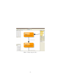
yED editor. The yED editor can either be downloaded from the website and
run as a standalone Java application, or be launched from the website directly
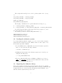
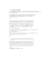
without installation (See Figure 1).
Once yED is up and running, we load the file trace.graphml. However, at
this moment the file contains only raw data of the query trace, and the initial
visualisation is not readable at all. We need to use several features of the yED
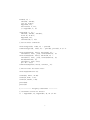
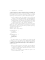
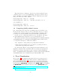
editor to improve it. This is done through the following three steps:
1. Select Tools, then Fit Node to Label..;
2. Select Tools, then Fit Label to Node.. (See Figure 2);
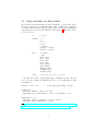
3. Select Layout, then Tree (See Figure 3).
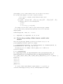
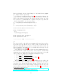
After these simple steps, the query trace is visualised as a tree, where each
node represents a state containing intermediate computational data such as
remaining goals, collected abducibles and collected constraints, and each edge
shows the goal selected for reduction during an abductive inference step. The
users can then zoom out/in to inspect the trace (see Figure 4), or even change
the appearance and layout of it.
5 downloadable
from https://www-dse.doc.ic.ac.uk/cgi-bin/moin.cgi/abduction?
action=AttachFile&do=view&target=circuit-diagnosis-2.pl
12
Figure 1: Launching yED Graph Editor
5
Acknowledgement
We would like to thank Domenico Corapi 6 , Srdjan Marinovic 7 , Dr. Robert
Craven 8 , and Prof. Antonis Kakas 9 for testing and features suggestions.
References
[1] Marc Denecker and Antonis C. Kakas Abduction in Logic Programming
Computational Logic: Logic Programming and Beyond 2002: 402-436
[2] Bert van Nuffelen and Antonis Kakas A-system: Declarative Programming
with Abduction Logic Programming and Non-Motonic Reasoning, vol. 2173,
393-397, 2001
[3] A. Kakas, B. Van Nuffelen, and M. Denecker A-system : Problem solving
through abduction Proceedings of the Seventeenth International Joint Conference on Artificial Intelligence (B. Nebel, ed.), vol. 1, Morgan Kaufmann
Publishers, Inc, 2001, pp. 591-596.
[4] S.Russell and P.Norvig Artificial Intelligence: A Modern Approach Prentice
Hall International, 1995.
6 http://www.doc.ic.ac.uk/
~dcorapi/
~srdjan/
8 http://www.doc.ic.ac.uk/ rac101/
~
9 http://www2.cs.ucy.ac.cy/ antonis/
~
7 http://www.doc.ic.ac.uk/
13
Figure 2: Resizing the Nodes
Figure 3: Layout the Trace as a Tree
14
Figure 4: Inspecting the Trace
15