Download USER'S GUIDE for DSM@MIT

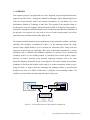
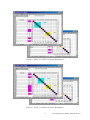
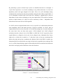
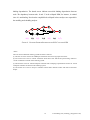
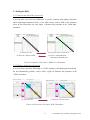
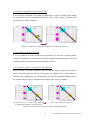
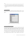
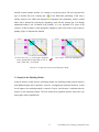
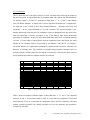
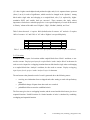
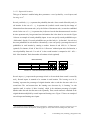
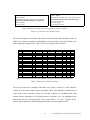
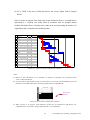
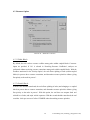
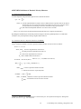
USER’S GUIDE for DSM@MIT
TABLE OF CONTENTS
1. OVERVIEW .....................................................................................................................3
2. INSTALLATION ..............................................................................................................5
3. FUNCTIONS....................................................................................................................7
3.1 Inputs for the Structuring Module ..................................................................................7
3.2 Analyses in the Structuring Module ...............................................................................8
3.3 Editing the DSM ........................................................................................................13
3.3.1 Insert a new task in the current row.......................................................................13
3.3.2 Delete a task in the current row ............................................................................13
3.3.3 Delete a dependency mark from the DSM.............................................................14
3.3.4 Undelete the mark in the DSM .............................................................................14
3.3.5 Swap the sequence of two tasks in the same level..................................................14
3.3.6 Move tasks with nonzero level slack.....................................................................15
3.3.7 Enter block names ...............................................................................................16
3.3.8 Insert the unplanned iteration mark.......................................................................16
3.4 Inputs for the Modeling Module ..................................................................................17
3.4.1 Durations ............................................................................................................18
3.4.2 Resources ...........................................................................................................19
3.4.3 Iteration ..............................................................................................................20
3.4.3.1 Sequential Iteration .......................................................................................21
3.4.3.2 Overlapping .................................................................................................22
3.5 Analyses in the Modeling Module ...............................................................................23
3.5.1 Analyses Results for Coupled Blocks ....................................................................23
3.5.2 Analyses Results for the Project ...........................................................................24
3.6 Transferring Analyses Results from the Structuring & Modeling Modules to the
Scheduling Module ...........................................................................................................26
4. OPTIONS........................................................................................................................28
4.1 Display Option...........................................................................................................28
4.1.1 Column Size .......................................................................................................28
4.1.2 Border ................................................................................................................28
4.1.3 Conversion in ‘Analysis’ Sheet.............................................................................29
4.2 Resource Option ........................................................................................................30
4.2.1 Within Blocks .....................................................................................................30
4.2.2 Outside Blocks ....................................................................................................30
4.3 Simulation Option......................................................................................................31
4.3.1 Latin Hypercube Sampling...................................................................................31
4.3.2 Task Duration Estimate Percentiles.......................................................................31
4.3.3 Direct Duration Inputs for Coupled Blocks............................................................32
4.3.4 Rework-Adjusted Durations and RPWs ................................................................32
4.3.5 Rework Risk Tolerance........................................................................................32
4.4 Gantt Chart & Table Option ........................................................................................33
4.4.1 Simulated Gantt Chart .........................................................................................33
4.4.2 MS Project Table .................................................................................................33
APPENDIX: DEFINITIONS OF HEURISTIC PRIORITY MEASURES.................................34
A1. Rank Positional Weight (RPW)...................................................................................34
A2. Cumulative Resource Equivalent Duration (CUMRED) ...............................................34
1
© Soo-Haeng Cho ([email protected])
2
© Soo-Haeng Cho ([email protected])
1. OVERVIEW
This computer program is an application tool of the integrated project management framework
proposed in the M.S. thesis, “An Integrated Method for Managing Complex Engineering Projects
Using the Design Structure Matrix and Advanced Simulation” by Soo-Haeng Cho at the
Massachusetts Institute of Technology in June 2001. The copyright of this program belongs to
Soo-Haeng Cho, Steven D. Eppinger, and Massachusetts Institute of Technology. This program is
protected by copyright law and international treaties. Unauthorized reproduction or distribution of
this program, or any portion of it, may result in severe civil and criminal penalties, and will be
prosecuted to the maximum extent possible under the law.
The integrated method streamlines project planning and control using three modules: structuring,
modeling, and scheduling, as illustrated in Figure 1. In the structuring module, the design
structure matrix (DSM) method is used to structure the information flows among tasks and
capture the iteration loops. By classifying various types of information dependencies, a critical
dependency path is identified and redundant constraints are removed for the modeling and
scheduling analyses. In the modeling module, a generalized process model predicts complex
behaviors of iterative processes using advanced simulation techniques such as the Latin
Hypercube Sampling and parallel discrete event simulation. The model computes the probability
distribution of lead time and identifies critical paths in a resource-constrained, iterative project.
Using the results of analyses from the structuring and modeling modules, a network-based
schedule in the form of a PERT or Gantt chart is developed in the scheduling module. The
schedule is used as the basis for monitoring and control of the project.
300
1
0.9
0.8
0.7
0.6
0.5
0.4
0.3
0.2
0.1
0
250
200
Structuring
Modeling
150
100
50
0
119.1
134.7
150.3
165.9
181.5
197.1
Scheduling
FIGURE 1. AN INTEGRATE PROJECT M ANAGEMENT FRAMEWORK
3
© Soo-Haeng Cho ([email protected])
The primary goal of this work is to develo p an integrated method that guides project management
efforts by improving the effectiveness and predictability of complex processes. The method can
also be used for identifying leverage points for process improvements and evaluating alternative
planning and execution strategies. Better project management will ultimately result in a better
quality product with timely delivery to customers.
The structuring and modeling modules are implemented as a Microsoft Excel Add-In. The
analyses results from these modules can be transferred to the structuring module in Microsoft
Project. Table 1 summarizes the inputs and analyses results of each module.
Inputs
•
•
•
Analyses Results
A list of tasks
Information flows among tasks
Information flow patterns
•
•
Structuring
•
•
•
•
•
Modeling
•
Duration estimates of tasks
Resource requirements of tasks
and capacity of the project
Dynamic characteristics of
overlapping and sequential
iterations (including the learning
curve)
Rework risk tolerance
•
•
•
•
•
Scheduling
•
Scheduled durations of tasks and
coupled blocks chosen from the
probability distribution
Due date and/or project buffer size
•
•
Design Structure Matrix
(Identification of loops and
process hierarchies among tasks)
Differentiation of planned &
unplanned iterations
Identification of non-binding
dependencies
A critical dependency sequence
and level slack of tasks
Probability distributions of the
durations of the project and
coupled blocks
Resource-constrained (or
conventional) slack and
criticalities of tasks
Critical sequences (or paths) with
percentages of criticalities
Simulated Gantt charts
PERT or Gantt chart
Schedule risk that the project fails
to meet the due date (or target)
Table 1. Summary of Inputs & Analyses Results of Modules
4
© Soo-Haeng Cho ([email protected])
2. INSTALLATION
For proper installation, a user must have two program files, one jpg file , and one excel file having
a sample application. The tool consists of three parts:
a. ‘[email protected]’ file: an add-in to Microsoft Excel
b. ‘[email protected]’ file: a module in Microsoft Project
c. ‘DSM to Gantt Chart’: a map for a file transfer from Microsoft Excel to Microsoft Project
Installation will be completed following the below four steps:
STEP1. Save ‘warning sign.jpg’ file under ‘C:/DSM/’.
STEP2. Install ‘[email protected]’ file.
(1) Start Microsoft Excel.
(2) Go to Tools – Add-ins – Browse.
(3) Select ‘[email protected]’ from the folder in which you saved this file.
STEP3. Install ‘[email protected]’ file.
(1) Start Microsoft Project.
(2) Go to Tools- Macro- Visual Basic Editor.
(3) Go to View- Project Explorer in the Visual Basic Editor.
(4) Choose ‘Modules’ folder under ‘ProjectGlobal(GLOBAL.MPT)’ in the Project Explorer
Window.
(5) Right-click and choose ‘Import File…’ and select ‘[email protected]’ from the folder in
which you saved this file.
STEP4. Create a map ‘DSM to Gantt Chart’ in Microsoft Project.
(1) Start Microsoft Project.
(2) From Menu, choose ‘Open’. Select ‘Microsoft Excel Workbooks’ from the drop-down
menu ‘Files of type’ and then the excel file containing a sample application. Open the
file.
(3) Click ‘New Map’.
(4) Type ‘DSM to Gantt Chart’ in the ‘Import/Export map name’ field and check ‘Tasks’,
‘Resources’ and ‘Export header row/Import includes headers’ in the ‘Option’ tab. Click
‘O.K.’.
5
© Soo-Haeng Cho ([email protected])
(5) In the ‘Task Mapping’ tab, select ‘MS Project’ from the drop-down menu of ‘Source
worksheet name:’. Match the fields ‘From: Worksheet Field’ to ‘To: Microsoft Project’
as follows:
To: Microsoft Project
From: Worksheet Field
ID
Task ID
Name
Task Name
Duration
Likely Duration
Predecessors
Predecessors
Resource Names
Resource Names
Priority
Priority
<Note> Make sure deselect ‘% Complete’ from the ‘Worksheet Field’.
(6) In the ‘Resource Mapping’ tab, select ‘Resource’ from the drop-down menu of ‘Source
worksheet name:’. Match the fields ‘From: Worksheet Field’ to ‘To: Microsoft Project’
as follows:
To: Microsoft Project
From: Worksheet Field
Name
Resource Name
Group
Group
Max Units
% Max. Units
(7) Click ‘O.K.’ and ‘Open’.
6
© Soo-Haeng Cho ([email protected])
3. FUNCTIONS
When Microsoft Excel starts, the add-in also starts automatically after proper set-up. The menu
“DSM” is located among standard menus in Excel, as shown in Figure 2. A user can perform
analyses for different projects using different workbooks at the same time. He can also save a
workbook and perform further analyses based on the data and analyses results stored earlier. The
tool receives inputs from a user through formatted worksheets. The inputs and analyses results of
each of three modules are explained in the following sections.
FIGURE 2. ADD-IN M ENU IN EXCEL
3.1 Inputs for the Structuring Module
By executing ‘New DSM’ in the menu, a user is given the ‘DSM Input’ worksheet which is
formatted for receiving inputs of maximum 240 tasks for the structuring module. A project name
in cell ‘2A’ must be unique to analyze different projects in other workbooks at the same time. For
analyses in the structuring module, a list of tasks and information flows among tasks are required.
First, list the tasks down in the first column in their rough sequence of execution with unique
indices. The same indic es are listed in the row above the square matrix.
The tool receives two types of information flows between tasks as shown in Figure 3. The first
type represents the case that a downstream task requires final output information from an
upstream task to begin its work. The second type represents the case that a downstream task uses
final output information in the middle of its process and/or begins with preliminary information
but also receives a final update from an upstream task.
7
© Soo-Haeng Cho ([email protected])
a
a
b
b
(a) First Type
(b) Second Type
FIGURE 3. TYPES OF INFORMATION FLOW BETWEEN TWO TASKS
When there is the first type of information flow from task a to task b, enter ‘1’ into (i, j) of the
square matrix where i and j are the unique indices representing tasks b and a, respectively. For the
second type of information flow, enter ‘2’. Reading across a row reveals the tasks where the
inputs of the task corresponding to the row come from. Reading down a specific column reveals
the tasks receiving outputs from the task corresponding to the column. If the sequence of tasks in
the matrix is the sequence of execution, a nonzero element in the upper diagonal represents a
feedback. Figure 4 shows a sample of the inputs for the structuring module.
FIGURE 4. INPUTS FOR S TRUCTURING M ODULE
3.2 Analyses in the Structuring Module
By executing ‘Analyze DSM’ in the menu, the tool performs analyses in the structuring module.
The results are shown in the five worksheets: ‘AEAP’, ‘ALAP’, ‘AEAP collapsed’, ‘ALAP
collapsed’, and ‘Analysis’. Figures 5 through 7 show the analyses results of the sample in Figure
4.
8
© Soo-Haeng Cho ([email protected])
FIGURE 5. ‘AEAP’ AND ‘AEAP COLLAPSED ’ WORKSHEETS
FIGURE 6. ‘ALAP’ AND ‘ALAP COLLAPSED ’ WORKSHEETS
9
© Soo-Haeng Cho ([email protected])
By partitioning a project, iteration loops (cycles) are identified and tasks are rearranged. A
coupled block represents a set of tasks constituting a loop, within which there is at least one
dependency mark in the upper diagonal of the matrix. Due to its cyclic relationships among
constituent tasks, iterations may take place potentially among the tasks within a coupled block. A
level is determined such that tasks in the same level constitute a coupled block or they are
independent of other tasks not belonging to the same coupled block. This multi-level structure
presents a simple hierarchy of a project as well as concurrency of tasks – independent tasks
and/or blocks in the same level can work in parallel.
In ‘AEAP’, tasks are sequenced based on the as-early-as-possible rule which assumes that a task
starts immediately after all the inputs necessary to begin are available. In ‘ALAP’, tasks are
sequenced based on the as-late-as-possible rule in which the starting time of a task is delayed to
the extent that it does not delay entire project. ‘AEAP collapsed’ and ‘ALAP collapsed’
worksheets show the collapsed views of the DSMs in ‘AEAP’ and ‘ALAP’, respectively, where
coupled blocks are collapsed to block tasks. In the collapsed views, information flow from a
single task to a block task is marked as ‘2’ when there exists at least one second-type flow
between the single task and any constituent task within the block in the DSM. In contrast, any
information flow from a block task to any single or block task is regarded as the second-type flow
as it is very likely that preliminary outputs of tasks within the block are transferred to downstream
tasks before converging to their final forms at the end of iterations.
FIGURE 7. ‘ANALYSIS’ WORKSHEET
10
© Soo-Haeng Cho ([email protected])
‘Analysis’ worksheet shows the results of structural analyses based on the AEAP collapsed DSM.
Level slack of a task is defined as the difference between its level in the ALAP DSM and that in
the AEAP DSM. Dotted boxes are wrapped around the columns of those tasks between the levels
they can be located in. For instance, “Block1” has level slack of two and it can be located
between levels two and four. The task ‘m’ and ‘Block2’ have nonzero level slack as well.
Various types of information dependencies are classified using the results of hierarchical
decompositions. A binding dependency represents the dependency which is regarded as a
constraint between two dependent tasks. The delay of information transfer directly causes the
downstream task to slip. This information dependency is translated to a precedence task
relationship of “finish-to-start” in the modeling and scheduling modules. All dependencies within
coupled blocks are regarded as binding. A non-binding dependency represents the dependency
which is not regarded as a constraint between two dependent tasks. The delay of information
transfer does not directly impact the schedule even though there is information flow between two
tasks. Thus, it is regarded as a redundant constraint and omitted in the modeling and scheduling
modules. A critical binding dependency is a binding dependency between the tasks with zero
level slack. A non-critical binding dependency is a binding dependency which is not criticalbinding. Following critical binding dependencies along the tasks, a critical dependency path goes
through the entire process hierarchies of a project from the first level to the last level. This path is
different from a critical path because it is determined without considering time aspects. However,
this path provides guidance for process improvements in the early stage of planning processes
when detailed data for durations are not available.
In Figure 7, the black or blue marks at (6,3), (8,4) , (10,6), (7,3) , and (10,5) represent non-binding
dependencies. The marks in first three cells are converted from ‘2’ in the AEAP collapsed DSM
to ‘1’ blue marks since there are no benefits from overlapping between downstream and upstream
tasks with non-binding dependencies. The pink marks at (3,1), (4,3), (7,4), (8,7) , (9,8) , and (10,9)
represent critical binding dependencies. The brown marks at (5,2), (6,4), (9,5) , and (9,6) represent
non-critical binding dependencies.
The network diagram in Figure 8 shows equivalent project structure of the AEAP collapsed DSM
except that non-binding dependencies are omitted. It is noticed that block tasks ‘B1’ and ‘B2’ as
well as singe task ‘m’ can be placed in different levels since they have nonzero level slack. The
path along the tasks ‘a-b-e-f-i-n-o’ is a critical dependency path of the project linked by critical
11
© Soo-Haeng Cho ([email protected])
binding dependencies. The dotted arrows indicate non-critical binding dependencies between
tasks. The dependency between tasks ‘b and ‘f’ in the collapsed DSM, for instance, is omitted
since it is non-binding. Note that the coupled blocks collapsed in these analyses are expanded in
the modeling and scheduling analyses.
f
b
e
B2
a
L(1)
i
B1
m
L(2)
L(3)
L(4)
L(5)
n
o
L(6)
L(7)
FIGURE 8. NETWORK DIAGRAM REPRESENTING AEAP COLLAPSED DSM
<Note>
The tool uses four different indexing systems for tasks as follows:
(1) The first one is the one used in ‘DSM Input' worksheet when receiving inputs from a user.
(2) The second one is used in ‘AEAP’ worksheet which shows new indices after partitioning. Indices in
‘ALAP’ worksheet are based on this indexing system.
(3) The third one is used in ‘AEAP collapsed’ worksheet after collapsing coupled blocks. Indices in ‘ALAP
collapsed’ worksheet are based on this indexing system.
(4) The fourth one is used in ‘Project’ worksheet which shows identical indices with IDs in Microsoft
Project.
12
© Soo-Haeng Cho ([email protected])
3.3 Editing the DSM
3.3.1 Insert a new task in the current row
A user can insert a new task from ‘DSM Input’ or ‘AEAP’ worksheet. After adding a task name
and its input/output information flows, a user must execute ‘Analyze DSM’ in the worksheet
where he has inserted the new task. Figure 9 illustrates this procedure in the ‘DSM Input’
worksheet.
(1) Select the row
(2) Execute ‘Insert a new task …’
(4) Execute ‘Analyze DSM’
(3) Enter a task name and
information dependencies
FIGURE 9. INSERTING A NEW TASK IN ‘DSM INPUT’ WORKSHEET
3.3.2 Delete a task in the current row
A user can delete a task from ‘DSM Input’ or ‘AEAP’ worksheet. After deleting the selected task,
the tool automatically performs ‘Analyze DSM’. Figure 10 illustrates this procedure in the
‘AEAP’ worksheet.
(1) Select the row
(2) Execute ‘Delete a task …’
FIGURE 10. DELETING A TASK FROM ‘AEAP’ WORKSHEET
13
© Soo-Haeng Cho ([email protected])
3.3.3 Delete a dependency mark from the DSM
A user can delete a dependency mark from the ‘DSM Input’ or ‘AEAP’ worksheet. After deleting
the selected mark, the tool automatically performs ‘Analyze DSM’. Figure 11 illustrates this
procedure in the ‘AEAP’ worksheet.
(1) Select the dependency mark
(2) Execute ‘Delete a dependency …’
FIGURE 11. DELETING A DEPENDENCY M ARK FROM ‘AEAP’ WORKSHEET
3.3.4 Undelete the mark in the DSM
A user can undelete the marks which have been deleted up to ten before executing another
command. This function is useful when a user wants to compare different partitioning results with
a certain dependency being assumed to be minimal and removed.
3.3.5 Swap the sequence of two tasks in the same level
From the ‘AEAP’ or ‘ALAP’ worksheet, a user can swap the sequence of the two tasks both of
which are located in the same level but do not belong to a coupled block, or both of which are
within the same coupled block. This command does not affect the partitioning results except for
this sequence change. Figure 12 illustrates this procedure in the ‘AEAP’ worksheet.
(1) Select the cell (i, j) in the lower diagonal
to change the sequence of tasks i and j
(2) Execute ‘Swap the sequences …’
FIGURE 12. S WAPPING TASK S EQUENCES FROM ‘AEAP’ WORKSHEET
14
© Soo-Haeng Cho ([email protected])
3.3.6 Move tasks with nonzero level slack
A task with nonzero level slack can be placed in a different hierarchy between its level in the
AEAP DSM and that in the ALAP DSM without affecting the structure of the project. If the task
is planned to start with some lag (i.e. later than the as-early-as-possible schedule ), the DSM can
show the better structure of the project by moving it to the level where tasks in the same level are
possibly performed in parallel with it. The tool allows a user to move those tasks and create
different DSM views in ‘Customized’ and ‘Cus. collapsed’ worksheets. This command must be
executed in the ‘Analysis’ worksheet as illustrated in Figure 13.
(1) Select the cell (i, j) where task j with nonzero level slack is going to be moved downstream
to the level of task i within a dotted box.
(2) Press ‘Ctrl’ and select other cells to be moved at the same time.
(3) Execute ‘Move tasks with nonzero …’.
FIGURE 13. MOVE TASKS WITH NONZERO LEVEL S LACK
15
© Soo-Haeng Cho ([email protected])
<Note>
(1) The tool assumes that the sequence of coupled blocks remains the same after moving tasks with
nonzero level slack. For instance, the index of block 1 should always be smaller than that of block 2.
(2) If a successor of a selected task also has nonzero level slack and its level is not higher than the target
level of the selected task, the successor is also moved to the level which is higher by one than the
target level.
3.3.7 Enter block names
Without entering the names of coupled blocks manually to all different worksheets, a user can
enter those names once to the form provided when executing ‘Enter Block Names’ as shown in
Figure 14.
FIGURE 14. ENTER THE NAMES OF COUPLED BLOCKS
3.3.8 Insert the unplanned iteration mark
The tool assumes that planned iteration only occurs between the overlapped tasks or tasks within
coupled blocks. Unplanned iteration represents a possible iteration in a system level or between
major development phases (usually a long feedback loop in the DSM), which is not accounted in
a project plan. The loop usually feeds back from the task such as major testing or reviewing at the
end of each phase. This can also be caused by unexpected market changes, technology innovation
etc. in the middle of processes. The unplanned iteration is often regarded as a failure mode and
requires managerial decision about whether to continue or abandon the project. When it is
16
© Soo-Haeng Cho ([email protected])
decided to pursue another iteration, it is common to re-plan the project. The tool represents this
type of iteration flow with ‘warning sign’ (
) in the DSM after partitioning. If this loop is
initially marked in the DSM and determined as unplanned after partitioning, smaller coupled
blocks can be obtained by replacing the dependency mark with the warning sign. Even though
unplanned iteration is not accounted in the schedule, it is very important to be aware of the
existence of those iterations so that appropriate contingency plans can be made as part of project
planning. Figure 15 illustrates this function.
(1) Select the cell (i, j) in the upper diagonal
where unplanned iteration may occur to
task i when task j is finished
(2) Execute ‘Insert the unplanned …’
FIGURE 15. INSERT THE UNPLANNED ITERATION M ARK
3.4 Inputs for the Modeling Module
Using the analyses results from the structuring module, the modeling module performs analyses
with additional inputs such as durations, resources, overlapping and sequential iterations. A table
for the inputs to the modeling module is created in ‘Project’ and ‘Resource’ worksheets after the
analyses in the structuring module. The tool assumes that sequential iteration takes place only
among tasks within coupled blocks.
17
© Soo-Haeng Cho ([email protected])
3.4.1 Durations
Table 2 shows the part of the table created in ‘Project’ worksheet after analyzing the sample in
the previous section. A coupled block has its constituent tasks and a dummy task with indentation.
For instance, ‘Block 1:’ in Table 2 is composed of single tasks ‘c’, ‘d’, ‘g’ and ‘j’; and a dummy
task ‘(D) Block1 Duration’. A dummy task is used to represent the duration of a coupled block.
For each task, a user is asked to enter three estimated durations – optimistic, most likely, and
pessimistic – for its expected duration of one-time execution. The expected duration is the
duration between the start and end of its continuous work even though the task may iterate more
than once afterwards. If a task is in progress, a user is also asked to enter actual duration and
percentage of completion. In this case, the estimated durations must be for a remaining duration
of a task. If a task within a coupled block has been completed before and iterates, the actual
duration of first execution needs to be provided in ‘Act Duration’ and 100% in ‘% Complete’.
The actual duration of a coupled block including all constituent tasks can also be tracked in ‘Act
Duration’ of a dummy task. The percentiles of optimistic and pessimistic estimates can be set
from the ‘Options’ (default values are 10% and 90%, respectively). The tool also allows a user to
specify different percentiles for duration estimates of each task.
Task ID
1
2
3
4
5
6
7
8
9
10
11
12
13
14
15
16
17
18
19
Task Name
a
Block1:
c
d
g
j
(D) Block1 Duration
b
e
m
Block2:
h
k
l
(D) Block2 Duration
f
i
n
o
Opt Duration
Likely Duration Pess Duration % Complete
Act Duration
Predecessors
1
3FS
3
4, 5
1
8
2
9
12FS
13
9
16
10, 11, 17
18
Table 2. Project Table (from ‘Project’ worksheet)
Table 3 shows an example of duration inputs. It shows that tasks ‘a’, ‘b’, and ‘c’ are completed
and tasks ‘d’ and ‘e’ are currently worked on. Task ‘d’ is expected to be completed in 5 days most
likely from now. Task ‘m’ is expected to be completed in 4 days with 20% confidence. (Note that
without specified percentiles, the default percentiles are used for optimistic and pessimistic
estimates of each task).
18
© Soo-Haeng Cho ([email protected])
Task ID
Task Name
1
2
3
a
Block1:
c
4
5
6
d
g
j
Opt Duration
4
2
3
Likely Duration Pess Duration % Complete
5
4
5
8
6
9
7
8
9
b
e
5
6
8
10
m
4[20%]
7
10
Act Duration
100%
0
100%
4
50%
5
100%
50%
9
6
3
(D) Block1 Duration
<Note>
(1) The optimistic estimate must be smaller than or equal to the most like ly estimate, which must
be smaller than or equal to the pessimistic estimate.
(2) The percentage of completion must be between 0 and 100% but does not need to be accurate.
(3) A user can also enter duration estimates for coupled blocks directly to ‘Project’ worksheet
without computing them in the modeling module. This is further explained in the ‘Options’.
(4) There is no need of entering duration estimates in the rows such as ‘Block1:’ and in ‘Block2:’.
Table 3. Duration Inputs (from ‘Project’ worksheet)
3.4.2 Resources
The tool assumes that there exists a fixed resource pool throughout the entire project duration.
‘Resource’ worksheet is given for receiving data for this resource pool. Table 4 shows an
example where ‘% Max Units’ represents the total amount of each resource available for the
project.
Resource Name
A1
A2
B1
B2
Group
A
A
B
B
% Max Units
100%
200%
200%
100%
Table 4. A Resource Pool (from ‘Resource’ worksheet)
The tool receives a resource requirement of each task which is assumed to be constant over the
entire period the task is processed. It also takes the resource requirements for block tasks,
assuming that those resources are required over the entire period that all constituent tasks are
processed. When two or more tasks are competing for limited resources in a certain period of
time, the tool determines priorities by the heuristic rule s1 . Among tasks within a coupled block, a
task has a higher priority if: (1) it has been in process, (2) it has a higher user-specified priority,
1
See the Appendix for the definitions of the measures used in the heuristic rules. These measures are
computed when analyzing coupled blocks or a project with resource constraints.
19
© Soo-Haeng Cho ([email protected])
(3) it has a higher rework-adjusted rank positional weight, and (4) it is sequenced more upstream
(from (1) to (4) in order of significance, which can also be changed in the ‘Options’). Among
block and/or single tasks not belonging to a coupled block, rule (3) is replaced by ‘higher
cumulative RED’ and ‘smaller slack per successor’. These measures also imply relative
importance of tasks from a schedule perspective. A user-specified priority of a task can be entered
in ‘Priority’ column of the table out of ‘Highest’, ‘High’, ‘Medium’ (default), and ‘Low’.
Table 5 shows that task ‘c’ requires 100% (default) units of resource ‘A2’ and task ‘d’ requires
100% of resource ‘A1’ and 150% of ‘A2’ with a ‘Highest’ user-specified priority.
Task ID
Task Name
1
a
2
Block1:
3
c
4
d
…
…
…
…
…
Resource Names
A1, B1
A2
A1, A2[150%]
Priority
Highest
Table 5. Resource Requirements and User-Specified Priorities (from ‘Project’ worksheet)
3.4.3 Iteration
In order to receive inputs for iterations within coupled blocks from ‘Block’ worksheet, a user
needs to execute ‘Display input layout for coupled blocks’ under ‘Analyze Block ’ in the menu. In
order to receive inputs for overlapping iterations between block and/or single tasks not belonging
to a coupled block from ‘Analysis’ worksheet, he also needs to execute ‘Display overlapping
input layout for the project’ under ‘Analyze Project’ in the menu.
The tool assumes that planned rework of a task is generated due to the following causes:
•
receiving new information from overlapped tasks after starting to work with preliminary
inputs
•
probabilistic change of inputs when other tasks are reworked
•
probabilistic failure to meet the established criteria
The first cause gives rise to overlapping iteration, and the second and the third causes give rise to
sequential iteration. Parallel iteration of a limited number of tasks is simulated by combining
overlapping and sequential iteration.
20
© Soo-Haeng Cho ([email protected])
3.4.3.1 Sequential Iteration
This type of iteration is modeled using three parameters: rework probability, rework impact, and
learning curve2 .
Rework probability (i, j, r) represents the probability that task i does rework affected by task j in
rth iteration. In the case of i < j, it represents the feedback rework caused by the change of
information from downstream task j or by the failure of downstream task j to meet the established
criteria. In the case of i > j, it represents the feedforward rework that downstream task i needs to
do since upstream task j has generated new information after it has done its own rework. Figure
16 shows an example of rework probability inputs. A user can specify rework probabilities up to
‘5th Iteration’ directly. If rework probabilities are provided only in ‘1st Iteration’, the tool uses
the same probabilities in each iteration. Alternatively, a user can specify a percentage decrease of
probabilities in each iteration by entering a number between 0 and 100% in ‘% Decrease’
(optional). For instance, if task ‘h’ has 60% in ‘% Decrease’ without inputs in the 2nd iteration, a
rework probability from task ‘l’ to task ‘h’ in the second iteration is computed as 0.8 * 60% =
0.48. ‘Max Iteration#’ limits the number of iterations of tasks (optional).
<Rework Probability>
h
1st Iteration
9 10 11
9
0.8
2nd Iteration
9 10 11
9
0.5
k
l
10 0.8
0.3
11
0.4
10 0.4
0.1
11
0.2
Task Name
% Decrease
Max.Iteration#
……
FIGURE 16. REWORK PROBABILITY (FROM ‘BLOCK’ WORKSHEET )
Rework impact (i, j) represents the percentage of task i to be reworked when rework is caused by
task j. Rework impact is assumed to be constant in each iteration. The learning curve in ‘%
Learning’ represents the percentage of original duration when a task does the same work for a
second time. The tool assumes that the learning curve decreases by ‘% Learning’ in each
repetition until it reaches ‘% Max. Learning’ which is the minimum percentage of original
duration when the task does the same work repeatedly. Thus, rework amount is calculated as the
original duration multiplied by rework impact and learning curve. Figure 17 shows an example of
rework impact and learning curve inputs.
2
The tool takes an approach similar to Browning and Eppinger, “Modeling the Impact of Process Architecture on Cost
and Schedule Risk in Product Development”, Working paper, No. 4050, Sloan School of Management, MIT, 2000.
21
© Soo-Haeng Cho ([email protected])
Task Name
h
k
l
<Learning Curve>
<Rework Impact>
% Learning
% Max.Learning
9 10 11
80%
60%
9
0.5
50%
50%
10 0.8
0.5
60%
50%
11
0.8
<Note> ‘% Learning’ must be higher than or equal to ‘% Max. Learning’.
FIGURE 17. REWORK IMPACT AND THE LEARNING CURVE (FROM ‘BLOCK WORKSHEET )
3.4.3.2 Overlapping
The tool receives inputs for overlapping iteration between the tasks of which information flow is
marked as ‘2’ in the DSM. These inputs need to be provided from ‘Block’ worksheet for tasks
within a coupled block and ‘Analysis’ worksheet for other tasks. The overlap amount (i, j)
represents the planned overlap amount between tasks i and j and it is a fraction of the expected
duration of task i. This carries the assumption that the downstream task cannot be completed
before the upstream task finishes. The overlap impact (i, j) represents the expected overlap impact
when task i is overlapped with task j by the given maximum overlap amount. It is a fraction of
that amount. If it is equal to 1, it implies no benefit from overlapping. To implement overlapping
strategy, it should be reasonably less than 1 considering additional risk due to the evolution of
volatile preliminary information. Figure 18 shows an example of overlapping inputs between
tasks within a coupled block.
Task Name
h
k
l
<Overlap Amount> <Overlap Impact>
9 10 11
9 10 11
9
9
10 0.3
0.2
10 0.5
0.5
11
11
FIGURE 18. INPUTS FOR OVERLAPPING (FROM ‘BLOCK’ WORKSHEET )
22
© Soo-Haeng Cho ([email protected])
3.5 Analyses in the Modeling Module
Analyses are performed in two steps. First, it computes probability distributions for expected
durations of coupled blocks. Then, it analyzes an entire project with coupled blocks collapsed,
which have computed distributions and separate resource requirements.
3.5.1 Analyses Results for Coupled Blocks
Figure 19 shows an example of analyses results in ‘Block’ worksheet obtained by
executing ‘Compute durations of coupled blocks’ under ‘Analyze Block’.
BLOCK2
# of simulation runs
100
1
80
0.8
60
0.6
40
0.4
20
0.2
0
0
1.4
5.6
9.8
14.0
18.2
22.4
26.6
cumulative probability
Duration: Avg 11.7 Std 2.9
(10%,30%,50%,70%,90%) = (8.4, 10.1, 11.5, 13, 15.3)
FIGURE 19. ANALYSES RESULT FOR COUPLED BLOCKS FROM THE M ODELING M ODULE
23
© Soo-Haeng Cho ([email protected])
The computed durations of a coupled block are also transferred to ‘Project’ worksheet, as shown
in Table 6. By default, 10th, 50th, and 90th percentiles of simulated durations are assigned to
optimistic, most likely and pessimistic durations of a dummy task, respectively.
Task ID
Task Name
11
Block2:
12
h
13
k
14
l
15
(D) Block2 Duration
Opt Duration
Likely Duration Pess Duration % Complete
3
1
2
8.4
4
2
3
11.5
Act Duration
6
3
4
15.3
Table 6. Simulated Durations of a Block Task in ‘Project’ Worksheet
The tool also draws three simulated Gantt charts out of many scenarios for ith block in ‘Gantt
Chart(Bi)’ worksheet. Figure 20 shows an example of a simulated Gantt chart. ‘Sampled
Duration’ represents the duration of one-time execution sampled from the triangular distribution
based on the estimated durations and percentiles. ‘Simulated Duration’ represents a total duration
including rework. The number inside a bar indicates the overlap amount of a task executed in
prior state(s).
<Scenario 2 of Block 2>
Task ID
12
13
14
Task Name Sampled Duration Simulated Duration
h
2.6
3.8
k
6.0
10.8
l
3.3
3.3
State
1
State Duration
2.6
Lead Time
17.9
2
6.0
3 4
3.3 1.2
5
4.8
<Note> Be careful not to print all ‘Block’ worksheet since there exist data not seen in the screen.
FIGURE 20. A SIMULATED GANTT CHART OF A COUPLED BLOCK
3.5.2 Analyses Results for the Project
Figure 21-22 and Table 7 show an example of analyses results in the ‘Project’ worksheet obtained
by executing ‘Compute lead time with resource constraints’ under ‘Analyze Project’. Figure 21
shows the summary of lead time computations, and major critical paths and sequences (resourceconstrained critical paths) with percentages that they are critical out of many simulation runs.
Note that lead time as well as critical paths are different when the tool accounts for resource
constraints from those without resource constraints. The tool also computes probability
distributions of the lead time with and without resource constraints.
24
© Soo-Haeng Cho ([email protected])
Lead Time (with Leveled Resources)
Avg 51.3, Std 8.3
(10%,30%,50%,70%,90%) = (41.8, 46.5, 50.3, 54.2, 61.9)
Major Critical Sequences (with Leveled Resources)
9-11-10-17-18-19 [69%]
2-10-18-19 [18%]
9-11-17-10-18-19 [10%]
Lead Time (without Resource Constraints)
Avg 44.8, Std 9.6
(10%,30%,50%,70%,90%) = (35.2, 39.5, 43.3, 48, 56.9)
Major Critical Paths (without Resource Constraints)
2-10-18-19 [52%]
9-11-18-19 [47%]
<Note> Task indices are based on the indexing system in ‘Project’ worksheet.
FIGURE 21. LEAD TIME AND CRITICAL PATHS
The tool also computes conventional and resource-constrained slacks and criticalities of tasks. In
addition, the measures computed for determining resource priorities are provided which reveal
relative importance between tasks. Table 7 shows an example of these measures.
Task ID
1
2
3
4
5
6
7
8
9
10
11
12
13
14
15
16
17
18
19
Task Name
a
Block1:
c
d
g
j
(D) Block1 Duration
b
e
m
Block2:
h
k
l
(D) Block2 Duration
f
i
n
o
…
…
…
…
…
…
…
…
…
…
…
…
…
…
…
…
…
…
…
…
Slack(avg,sd)
%Criticality RC_Slack(avg,sd) %RC_Criticality CUMRED
RED
Slack/Suc
3.6, 5.7
53
7.3, 7.3
20
7.0
0.0
0.0
5, 7.8
3.6, 5.7
5, 7.8
47
53
47
1.5, 4.9
0, 0
1.5, 4.9
80
100
81
22.3
7.0
19.3
0.0
7.0
19.3
0.5
0.0
1.2
15.9, 8.6
15.9, 8.6
0, 0
0, 0
0
0
100
100
20.4, 7.9
1.5, 4.9
0, 0
0, 0
0
81
100
100
3.0
3.0
0.0
0.0
0.0
3.0
0.0
0.0
4.6
6.9
0.0
0.0
<Note> Be careful not to print all ‘Project’ worksheet since there exist data not seen in the screen.
Table 7. Measures for Task Criticalities
The tool also draws three simulated Gantt charts out of many scenarios in ‘Gantt Chart(P1)’
worksheet for the results without resource constraints and in ‘Gantt Chart(P2)’ worksheet for the
results with resource constraints. Figure 22 shows the examples of a simulated Gantt Chart
without resource constraints in (a) and with resource constraints in (b). The highlighted tasks
indicate that they are on critical path(s). In (b), tasks ‘Block2’, ‘m’, and ‘i’ compete for the
limited resource and the tool determined priorities based on the rules explained earlier.
25
© Soo-Haeng Cho ([email protected])
Task ID Task Name Simulated Duration
1
2
a
Block1:
8
9
b
e
0.0
19.1
0.0
5.0
10
11
m
Block2:
10.0
16.2
16
17
f
i
4.8
4.7
18
19
n
o
8.8
6.4
State
State Duration
1
5.0
Total Lead Time
44.3
2
4.8
3
4.7
4 5
4.6 2.1
6
7.9
7
8.8
8
6.4
(a) Without Resource Constraints
Task ID Task Name Simulated Duration
1
2
8
a
Block1:
b
0.0
19.1
0.0
9
10
e
m
5.0
10.0
11
16
Block2:
f
16.2
4.8
17
18
19
i
n
o
4.7
8.8
6.4
State
State Duration
Total Lead Time
1
5.0
2
4.8
3 4
9.3 2.1
5
10.0
6
4.7
7
8.8
8
6.4
51.1
(b) With Resource Constraints
<Note> Tasks ‘a’ and ‘b’ are completed, and ‘Block1’ and ‘e’ are in progress.
FIGURE 22. SIMULATED GANTT CHARTS OF A PROJECT
3.6 Transferring Analyses Results from the Structuring & Modeling Modules to the
Scheduling Module
When executing ‘Analyze Project’, the tool creates ‘MS Project’ worksheet. Using the data map
created in ‘INSTALLATION’ section, a user can transfer the data in this worksheet to Microsoft
Project as follows:
(1) Start Microsoft Project.
(2) From Menu, choose ‘Open’. Select ‘Microsoft Excel Workbooks’ from the drop-down
menu ‘Files of type’ and then the excel file having analyses results from the structuring and
modeling modules. Open the file.
(3) Choose ‘DSM To Gantt Chart’ for ‘Import/Export map to use for importing:’ and ‘Open’.
Then, a user must have a Gantt chart in Microsoft Project.
26
© Soo-Haeng Cho ([email protected])
(4) Go to ‘DSM’ in the menu of Microsoft Project and execute ‘Adjust Tasks in Coupled
Blocks’
Figure 23 shows an example of the Gantt chart created in Microsoft Project. A coupled block is
represented as a ‘rolled-up’ task within which its constituent tasks are arranged without
feedback information flows. A dummy task is added at the end representing the duration of a
coupled block that is computed in the modeling module.
ID
1
Task Name
a
Duration Predecessors
5 days
2
Block1:
3
c
4 days
4
d
10 days 3
5
g
4 days 3
6
j
7
(D) Block1 Duration
5/13
5/20
5/27
June
6/3
6/10
6/17
6/24
July
7/1
7/8
7/15
7/22
August
7/29
8/5
8/12
8/19
27.1 days 1
5 days 4,5
27.1 days
8
b
6 days 1
9
e
9 days 8
10
m
11
Block2:
12
h
4 days
13
k
5 days 12
14
l
15
(D) Block2 Duration
7 days 2
A
18.5 days 9
5 days 13
18.5 days
16
f
5 days 9
17
i
3 days 16
18
n
8 days 10,11,17
19
o
5 days 18
A
A
FIGURE 23. A GANTT CHART IN M ICROSOFT PROJECT
<Note>
(1) Make sure that ‘Calculation’ is set ‘Automatic’ as default in ‘Calculation’ tab of ‘Options’ under
‘Tools ’ in Microsoft Project.
(2) If a project has a small number of tasks as shown below, a user needs to delete additional rows other
than the rows with task names before executing ‘Adjust Tasks in Coupled Blocks’.
Needs to be
deleted
FIGURE 24. ADJUSTMENT IN MICROSOFT PROJECT
(3) When a project is in progress, actual durations of tasks are not transferred to MS Project. For
completed tasks, a user needs to change durations from 1 to 0 in MS Project.
27
© Soo-Haeng Cho ([email protected])
4. OPTIONS
4.1 Display Option
FIGURE 25. ‘DISPLAY’ OPTION
4.1.1 Column Size
This option gives a user to adjust cell sizes in worksheets directly. ‘DSM entry cell’ is the width
of cells in the DSM. ‘Level column’ is the width of columns showing levels. ‘Task name column’
is the width of columns showing task names. ‘Gantt Chart unit bar’ is the width of a bar for one
unit of duration in simulated Gantt charts.
4.1.2 Border
If the first checkbox is selected, the tool draws borders around diagonal cells in the DSM, as
shown in Figure 26. With the second checkbox selected (by default), the tool draws borders when
running ‘Analyze DSM’, as shown in Figure 27.
28
© Soo-Haeng Cho ([email protected])
index of a task
(a) In the Worksheet ‘DSM Inputs’
a
Task Name
Level
1
1
1
1
2
3
c
d
2
2
2
3
2
2
2
3
g
j
2
2
4
5
1
b
e
m
2
3
3
6
7
8
1
h
4
9
4
5
6
7
1
1
1
4
1
1
8
9
Block1
5
1
6
1
7
2
1
1
8
9
(b) In the Worksheet ‘AEAP’
FIGURE 26. BORDERS AROUND DIAGONAL CELLS
a
c
Task Name
Level
1
2
1
2
1
d
g
2
2
3
4
1
j
b
2
2
5
6
1
e
3
7
2
3
4
2
5
6
7
borders
1
2
1
1
1
1
1
FIGURE 27. BORDERS IN DSM VIEWS
4.1.3 Conversion in ‘Analysis’ Sheet
As explained in ‘Analyze DSM’, if non-binding dependencies between tasks are marked as ‘2’ in
AEAP and ALAP collapsed views, they are converted from ‘2’ to ‘1’ blue marks in the
‘Analysis’ worksheet by default. With this checkbox unselected, the tool does not make these
automatic conversions.
29
© Soo-Haeng Cho ([email protected])
4.2 Resource Option
FIGURE 28. ‘RESOURCE’ OPTION
4.2.1 Within Blocks
By default, the tool resolves resource conflicts among tasks within coupled blocks if resource
inputs are provided. If ‘No’ is selected in ‘Resolving Resource Confliction’, analyses are
performed without resolving resource constraints among tasks within coupled blocks. With the
checkbox unselected in the ‘Priority Option’, the tool allows splitting of tasks (within coupled
blocks) in process due to resource constraints, and determines resource priorities without ‘giving
first priority to the tasks in process’.
4.2.2 Outside Blocks
With the first checkbox unselected, the tool allows splitting of tasks (not belonging to a coupled
block) in process due to resource constraints, and determines resource priorities without ‘giving
first prior ity to the tasks in process’. With this option, the tool does not compute slack and
criticalit ies of tasks, and major critical sequences. With the second checkbox unselected, the tool
considers ‘slack per successor’ before CUMRED when determining resource priorities.
30
© Soo-Haeng Cho ([email protected])
4.3 Simulation Option
FIGURE 29. ‘S IMULATION’ OPTION
4.3.1 Latin Hypercube Sampling
The tool uses the Latin Hypercube Sampling (LHS) method 3 and assumes the triangular
probability distribution for the expected duration of a task. The LHS method divides the input
distribution into N1 (= ‘Number of strata in probability distribution’) strata of equal marginal
probability and randomly samples once from each stratum. Then, it sequences the sampled values
randomly. The tool repeats this procedure N 2 (= ‘Number of Latin Hypercube Sampling’) times.
Thus, it generates total N (= N1 × N 2 ) random numbers for each task. N is the total number of
simulation runs.
4.3.2 Task Duration Estimate Percentiles
‘Default % of optimistic value’ is a default percentile of optimistic duration estimates of tasks.
‘Default % of pessimistic value’ is that of pessimistic duration estimates.
3
McKay, M., Beckman, R. and Canover, W., “A Comparison of Three Methods for Selecting Values of Input
Variables in the Analysis of Output from a Computer Code.”, Technometrics, Vol. 21, No. 2, pp. 239-245, 1979.
31
© Soo-Haeng Cho ([email protected])
4.3.3 Direct Duration Inputs for Coupled Blocks
If ‘YES’ is selected, the tool uses user-specified duration estimates for coupled blocks instead of
computed durations from the modeling module . This option can be effectively used when a user
can estimate expected durations of coupled blocks more accurately than using the modeling
technique.
4.3.4 Rework-Adjusted Durations and RPWs
When analyses are performed with resource constraints, the tool computes rework-adjusted
durations and rank positional weights by default. With this option selected, it also computes them
when analyses are performed without resource constraints.
4.3.5 Rework Risk Tolerance
When tasks iterate sequentially, a choice of rework policy may allow rework concurrency to
shorten the lead time. For illustration, consider the simple example given in Figure 30. When both
tasks ‘a’ and ‘b’ require new information from task c, the work policy of performing the rework
of both tasks ‘a’ and ‘b’ concurrently may be preferred in order to shorten the lead time. In this
example, the tool assumes that they are reworked concurrently if the total rework probability
between the two tasks is less than a rework risk tolerance. If this is zero (default), a downstream
task always waits until the rework of an upstream dependent task is completed. (For more detail,
refer to the thesis written by Soo-Haeng Cho).
Task Name
a
b
c
(a) Information Flow Diagram
1
a
b
1
2
c
3
2
3
1
1
1
1
(b) DSM
FIGURE 30. AN EXAMPLE FOR TASK CONCURRENCY
32
© Soo-Haeng Cho ([email protected])
4.4 Gantt Chart & Table Option
FIGURE 31. ‘GANTT CHART & TABLE’ OPTION
4.4.1 Simulated Gantt Chart
If ‘NO’ is selected, the tool does not draw simulated Gantt charts for coupled blocks and/or a
project. This option saves computation time significantly.
4.4.2 MS Project Table
By default (with the first option selected), the tool creates ‘MS Project’ worksheet when
executing ‘Compute lead time with resource constraints’. With the second option selected, the
tool creates the worksheet when executing ‘Compute lead time without resource constraints’.
With the third option selected, the tool does not create the worksheet.
33
© Soo-Haeng Cho ([email protected])
APPENDIX: Definitions of Heuristic Priority Measures
A1. Rank Positional Weight (RPW)
A rework-adjusted rank positional weight of task i is defined as follows:
rpwi = d i +
∑d
j
j
where, di : rework-adjusted duration of task i which is defined as the expected value of the sum of
the duration of its first execution and the total amount of successive rework it creates
for its predecessors, assuming no resource constraints in the project network.
∑ d :j sum of all rework-adjusted durations over all successors of task i
j
(Note: a set of successors includes all downstream tasks that receive outputs from the task.)
By adding the summation part of the rank positional weight, it measures global importance of a task while
it measures only local importance among neighbor tasks without it.
A2. Cumulative Resource Equivalent Duration (CUMRED)
Cooper4 defined a cumulative resource equivalent duration of task i of each resource as follows:
RUDk = Lk + E k / Rk
where, RUDk : resource usage duration of resource k
Lk : last time period of requirement for resource k
E k : total excess requirement for resource k
Rk : total available amount of resource k
RUDMAX = Maximum{ RUDk } where k = 1, 2,…, K (number of resources)
REDi =
K
∑ (r
k =1
ik
/ Rk ) ⋅ ( RUD k / RUDMAX ) ⋅ d i
where, REDi : resource equivalent duration of task i
rik : amount of resource k required by task i
CUMRED i = RED i +
∑ RED
j
j
where, CUMREDi : cumulative resource equivalent duration of task i
RED : sum of RED over all successors of task i
∑
j
j
4
Cooper, D., “Heuristics for Scheduling Resource-Constrained Projects: An Experimental Investigation,” Management
Science, Vol. 22, No. 11, pp. 1186-1194, 1976.
34
© Soo-Haeng Cho ([email protected])