Download Wealth and Assets Survey User Guide

UK Data Archive Study Number 6415 - Wealth and Assets Survey: Special Licence Access
Wealth and Assets
Survey User Guide
1
CONTENTS
OVERVIEW ........................................................................................... 3
USING WEALTH AND ASSETS SURVEY DATA ......................................... 4
CONTENT OF DATA FILES ............................................................................................................................ 4
VARIABLE NAMING CONVENTIONS ............................................................................................................... 4
WEIGHTS ................................................................................................................................................ 4
INTERVIEW OUTCOME CODES ..................................................................................................................... 5
LONGITUDINAL DATA LINKAGE..................................................................................................................... 6
LONGITUDINAL FLAGS ............................................................................................................................... 7
VARIABLE SPECIFIC NOTES ................................................................... 8
SURVEY DESIGN ................................................................................... 9
SAMPLING STRATEGY ................................................................................................................................ 9
SAMPLE SIZES OF EACH WAVE ................................................................................................................... 10
WAVE STRUCTURE .................................................................................................................................. 10
MODE OF DATA COLLECTION..................................................................................................................... 11
Mainstage interview ..................................................................................................................... 11
Keep in Touch Exercise interview .................................................................................................. 11
FIELDWORK PROCEDURES .................................................................. 12
INTERVIEWER TRAINING ........................................................................................................................... 12
Generic interviewer training ......................................................................................................... 12
Survey specific training ................................................................................................................. 12
RESPONDENT CONTACT ........................................................................................................................... 13
FIELD SAMPLING PROCEDURES .................................................................................................................. 14
RESPONSE RATES ............................................................................... 15
KEEPING IN TOUCH ................................................................................................................................. 16
QUESTIONNAIRE CONTENT ................................................................ 17
QUESTIONNAIRE CHANGES ....................................................................................................................... 17
LENGTH OF QUESTIONNAIRE ..................................................................................................................... 18
PROGRAMMING AND TESTING................................................................................................................... 18
EDITING ............................................................................................. 21
IMPUTATION ...................................................................................... 23
GENERAL METHODOLOGY ........................................................................................................................ 23
DONOR SELECTION ................................................................................................................................. 24
PROCESSING STRATEGY ........................................................................................................................... 27
QUALITY ASSURANCE AND EVALUATION ..................................................................................................... 30
WEIGHTING ........................................................................................ 31
DATA QUALITY ................................................................................... 43
SAMPLING ERROR ................................................................................................................................... 43
NON-SAMPLING ERROR ........................................................................................................................... 43
EXTERNAL SOURCE VALIDATION ................................................................................................................. 44
WEALTH ESTIMATES ........................................................................... 46
CONTACT DETAILS .............................................................................. 50
2
Overview
The Wealth and Assets Survey (WAS) is a longitudinal survey that interviewed across Great
Britain; England, Wales and Scotland (excluding North of the Caledonian Canal and the Isles
of Scilly). Respondents to wave one (July 2006 – June 2008) of the survey were invited to
take part in a wave two follow up interview two years later (July 2008 – June 2010).
Respondents to wave 2 were then invited to take part in a wave three follow up interview
another two years later (July 2010 – June 2012). In addition to these follow up interviews, a
new random sample of addresses was also added at wave 3. Interviews in all waves were
conducted using Computer Assisted Personal Interviewing (CAPI). Wave one achieved
approximately 30,000 household interviews, wave two achieved approximately 20,000
household interviews and wave three achieved approximately 21,000 household interviews.
The economic well-being of a households is often measured by its income, and yet a
household's resources are composed of its stock of wealth as well as its flow of income. To
more fully understand the economic well-being of households it is necessary to look beyond
measures of household income.
The WAS addresses this gap in data about the economic well-being of households by
gathering information on the ownership of assets (financial assets, physical assets and
property), pensions, savings and debt.
The WAS is funded by a consortium of government departments: Department for Work and
Pensions; HM Revenues and Customs; HM Treasury; Office for National Statistics; and, the
Scottish Government. Fieldwork is undertaken by the Office for National Statistics.
3
Using Wealth and Assets Survey data
Content of data files
The data are split into two linked files:
(1) a household level file containing all property and physical wealth component
variables, as well as all derived variables (DV) used for the calculation of aggregated
household wealth and income.
(2) A person level file consisting of all person level financial wealth, pension wealth and
income component variables and DVs.
Variable naming conventions

Wave suffix
Variables in both datasets are given the suffix “W3” to indicate that they contain
values collected in wave 3. There are a few variables with the suffix “W2” or “W1”
and these contain values from wave 2 or wave 1. Most of the W2 and W1 variables
are present to allow the datasets to be matched to those from previous waves of the
survey, e.g. HHSERIALW2.

Imputation suffix
All variables used as components for wealth DVs were subject to imputation.
Variables that have had missing data imputed appear in the datasets in two versions.
The version that contains only the values observed at interview will end with the
suffix W3 as described above, e.g. FSInValW3. The version that contains both
observed and imputed values will end with the suffix ‘_i’, e.g. FSInValW3_i.

Aggregation suffix
To calculate total household wealth all component DVs were aggregated to
household level. To enable data users to use aggregated household level DVs on
person level, relevant DVs are also provided on the person level file.
Weights
To carry out cross-sectional analysis based on the individual wave data, the following table
has the appropriate variable weight to apply for cross-sectional analysis.
Wave
1
2
3
Cross-sectional Calibration Weight
XS_wgtW1
XS_calwgtW2
w3xswgt
4
As opposed to cross-sectional analysis, longitudinal analysis can only be carried out on
person level. The following table has the longitudinal variable weight to apply for
longitudinal analysis.
Wave
W1W2 Longitudinal Weight
W1W3 longitudinal weight
W2W3 longitudinal weight
Longitudinal Calibration Weight
Longit_calwgtW2
w1w3wgt
w2w3wgt
Interview Outcome codes
The datasets include responding households only. The variable HOutW3 gives an indication
of the type of interview outcome of the household:
Fully co-operating
110 Complete interview by required respondent(s) in person
120 Fully co-operating household: one or more interviews completed by proxy
121 HRP economic unit interviewed in person, one or more other interviews by proxy
122 HRP and/ or spouse/ partner interview by proxy
130 Complete interview by proxy
Partially co-operating
212 Non-contact with one or more respondents
213 Refusal by one or more respondents (all contacted)
214 All adults interviewed but one or more interviews was incomplete
222 Non-contact with one or more respondents and some proxy information
223 Refusal by one or more respondents (all contacted) and some proxy information
224
All adults interviewed but one or more interviews incomplete and some proxy
information
211 Full response in person from HRP economic unit – HRP (and spouse/ partner). One or
more other interviews missing or incomplete.
212 Full response from HRP economic unit – one or both by proxy. One or more other
interviews missing or incomplete.
220 HRP economic unit not complete (one of 2 eligible adults missed; either interview
incomplete).
230 No individual interviews with HRP economic unit but household interview completed.
Although the dataset exclusively consists of responding households, not every individual in
every household responds. The variable IOut1W3 indicates the interview outcome of
individuals:
1
2
3
4
5
6
Full interview (in person or by proxy)
Partial interview (in person or by proxy)
Ineligible for interview – child aged 0 to 15
Ineligible for interview – adult aged 16 to 18 in full-time education
Eligible adult – refused to be interviewed
Eligible adult – non-contact
5
Please note:
Although individuals with an outcome code of 5 or 6 did not give an interview they can still
be included in the analysis because their values for wealth component variables have been
imputed.
Also, analysts should be aware that although children have not been interviewed for this
survey, the data on children assets has been recorded against their person number in the
household, not against the adult who responded to the relevant questions in this section.
Longitudinal data linkage
All final data files are linked files have a single variable to use for linking cases between
waves. For household linking, there are separate variables for each wave; each case may
have up to three variables with a valid code. For person level there is one variable used for
matching a case in any wave.




Always used the linked file as a base when matching variables across waves.
Use HHSerialW1, HHSerialW2 and/or HHSerialW3 for household linking.
Use PIDNo for person level linking, this remains the same over the survey life time of a
sample unit.
When GETting the files, only KEEP the variables you need to add to the file (including the one
needed to match cases). This makes it easier when matching.
To add W2 variables to the W3 person file, keeping only W3 cases:
 Sort W1W2W3 person level linked files by PIDNo (W1W2W3_UKDA.sav)
 Sort W2 Person file by PIDNo
 Sort W3 Person file by PIDNo
 Match W2 and W3 files with the linked file being used as a look up TABLE; use PIDNo to
MATCH.
 This will add W2 variables to W2 cases and W3 variables to W3 cases
 Select the required cases e.g. for W3 cases (including linked W2 cases) use HHSerialW3 > 0.
To add W3 variables to the W2 household file, keeping all cases:
 Sort the linked file by HHSerialW2 (W1W2W3_UKDA.sav)
 Sort W2 household file by HHSerialW2
 Match files using HHSerialW2
 Sort the new file by HHSerialW3
 Sort W3 household file by HHSerialW3
 Match files using HHSerialW3
 This will produce a linked W2W3 file with W2 and W3 variables.
Linking within a wave
To add household variables to the W3 person file:
 Sort both files by HHSerialW3 and use this variable to MATCH
 Use the household file as a look up TABLE. This will add the household variables to each
person in the household.
6
Note: Person level variables cannot be added to the household file unless they are aggregated first.
Linking End User Licence (EUL) data
As the EUL datasets are anonymised the variables HHSerial and PIDNo have also been
anonymised. To link household files the variable Case replaces HHSerial, therefore Case will
need to be used when linking cases. To link person files the variable Person replaces PIDNo,
therefore variables Case and Person will need to be used when linking cases.
Linking using EUL datasets:


Use CaseW1, CaseW2 and/or CaseW3 for household linking.
Use PersonW1, PersonW2 and/or PersonW3 and CaseW1, CaseW2 and/or CaseW3 for
person level linking.
To add W2 variables to the W3 person file, keeping only W3 cases:
 Sort W2 by CaseW2 and PersonW2.
 Sort W3 by CaseW2 and PersonW2.
 Match W2 and W3; using PersonW2 and CaseW2 to MATCH.
 This will add linkable W2 cases to the W3 file and add W2 variables to W2 cases.
 Select the required cases e.g. for W3 cases (including linked W2 cases) use CaseW3 > 0.
To add W3 variables to the W2 household file, keeping all cases:
 Sort W2 household file by CaseW2
 Sort W3 household file by CaseW2
 Match files using CaseW2
 This will produce a linked W2W3 file with W2 and W3 variables.
Longitudinal Flags
A number of longitudinal flags have been produced that may help to understand changes in
the data when conducting longitudinal analysis with the linked data.
The following person level flags are only included on the person level datasets.
Type – Indicator for linkage status
1 = W1 – W3 Linked cases
(regardless interview eligibility and response status)
2 = W2 – W3 Linked cases
(regardless interview eligibility and response status)
3 = W3 HAK Joiner
Individual joined the household when keep-in-touch exercise was conducted
4 = W3 HAD Joiner
Individual joined the household when debtor survey was conducted
5 = W3 New respondents
Individual joined the household when W3 interview was conducted
6 = W3 New Household
Individual is part of a household that responded at W3 for the first time
7 = Individual no present at W3
This person was part of a responding household in W2 but left the household at W3
7
and did not respond
8 = Household not present at W3
Individual was part of a responding household in W2 but the whole household did not
respond at W3
P_Flag1W3 – Flag for wave member status
1 = LOSM
Longitudinal original sample member – individual was a member of a
responding household in W2 and W3
2 = EOSM
Entrant original sample member – individual was a member of a
responding household in W3, but household did not respond in W2
3 = SSM
Secondary sample member – individual was not a member of any
household in W2 but joined a longitudinal household in W3
4 = NSM
Non-responding sample member – individual was a member of a responding
household in W2 but left the sample at W3
P_Flag2W3 – Flag for wave entrant status
1 = OSM birth entrant
Child entrant (15years or younger) born to OSM household member
2 = SSM birth entrant
Child entrant (15years or younger) born to SSM household member
3 = Other SSM entrant
Adult entrant (16years or older)
P_Flag3W3 – Flag for wave eligibility status
1 = Eligible adult
Aged 16 years or older and not in full-time education
2 = Ineligible adult
Aged 16 to 18 years in full-time education
3 = Ineligible child
Aged 15 years or younger
P_Flag4W3 – Flag for HRP status
1 = HRP in W2 & W3
Individual was HRP in both waves
2 = HRP in W2, not W3
Individual was HRP in second but not in third wave
3 = HRP in W3, not W2
Individual was HRP in third but not in second wave
4 = Never HRP
Individual was never the HRP (inc. children)
Variable specific notes
Refer to the wave 3 paper questionnaire for notes on specific variables.
8
Survey design
Sampling strategy
The Wealth and Assets Survey collects information about private household wealth in Great
Britain. The survey uses the small users Postcode Address File (PAF) as the sample frame for
residential addresses in Great Britain, that is, England, Wales and Scotland; excluding North
of the Caledonian Canal and the Isles of Scilly. The ONS copy of the PAF is updated twice a
year to ensure that recently built addresses are included and demolished or derelict
properties are removed quickly.
The survey estimates are designed to be representative of the GB population, therefore
WAS, like most social surveys uses a ‘probability proportional to size’ or PPS method of
sampling cases. This means that the probability of an address being selected is proportional
to the number of addresses within a given geographic area, with a higher number of
addresses being selected from densely populated areas.
WAS uses a two-stage or ‘clustered’ approach to sampling. Firstly, postcode sectors are
randomly selected from the PAF. The postcode sectors are the primary sampling units (PSUs)
for the survey. Within each of these postcode sectors, 26 addresses are randomly selected.
The selection uses a stratified (ordered) PAF, where addresses are listed by postcode and
street number. The list of 26 addresses is split into two quotas of 13 addresses to ease the
allocation (to interviewers) and management of fieldwork.
The sampled PSUs were allocated to months at random. This was done using a repeating
random permutation which ensured that PSUs allocated to the same quarter and month
were evenly spread across the original sample, while still ensuring that each sampled PSU
had an equal chance of being allocated to each month. This even spread meant that monthly
and, particularly, quarterly samples were balanced with respect to the regional and censusbased variables used in the stratification.
Although the address selection within postcode sectors is random, some addresses have a
higher probability of selection than others. This reflects the fact that wealth has a heavily
skewed distribution with a relatively small number of addresses holding considerable
wealth. This skewed distribution of wealth, and the fact that it is often harder to secure
response from wealthier households is the reason for the over sampling of wealthy
addresses. For year one of wave one, addresses identified as having high wealth were 2.5
times more likely to be sampled than other addresses. This factor was increased to 3.0 for
the second half of wave one in order to further increase the number of achieved interviews
with high wealth addresses.
‘High’ wealth addresses are identified after the postcode sectors have been established. A
limited amount of information is available about the type of household resident at a
particular address on the PAF and what is generally available relates to the area around the
address, rather than being specific to an address. However, HMRC collects data on income
and certain components of wealth in order to administer the tax system and the SelfAssessment regime. Data from HMRC on tax returns at an address level, in conjunction with
9
average FTSE350 dividend yields from the previous calendar year are used to estimate the
value of share holdings at a household level. Those addresses estimated to be in the 90 th
percentile of shareholding value were then oversampled at a rate of 2.5 (wave one) or 3.0
(waves three and four – new cohort sample) relative to other addresses within a given
postcode sector.
Sample sizes of each wave
The following table provides a summary of the sample sizes (rounded), both issued and
achieved, for each of the first three waves of the Wealth and Assets Survey.
Wave
Issued addresses
One
62,800
Two
32,200
Three
37,900
*Respondents aged 16 and over.
Achieved
households
Achieved adults*
30,500
20,000
21,450
53,300
34,500
40,400
In developing the survey, precision targets for change on key estimates were agreed in
consultation with funding departments. From these, it was estimated that an overall
achieved sample of approximately 32,000 households, spread evenly over the two years of
wave one was required. In addition to the above precision targets there was a further target
to achieve a two-year sample of 4,500 households above the top wealth decile for wave one.
This was well above the 3,200 households that would be above the top wealth decile for an
equal probability sample. Oversampling the wealthiest households allows for more detailed
analysis of this group and gives more precise estimates of the levels of wealth across the
whole population.
For wave two, the achieved wave one sample was issued, plus all of the non-contacts. A total
of 32,200 addresses were issued for wave two.
In wave three, follow-up of the respondents and non-contacts at wave one and wave two
was supplemented by the introduction of a new random sample of around 12,000
addresses.
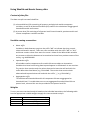
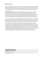
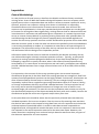
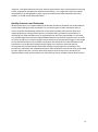
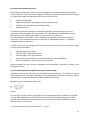
Wave structure
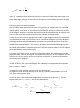
The following diagram illustrates the longitudinal design of the Wealth and Assets Survey.
Wave one started in July 2006 with fieldwork being spread over a two year period. Wave
two, a follow up to wave one was conducted between July 2008 and June 2010. The
introduction of a new cohort of addresses in wave three is shown in blue.
All interviews have a two yearly interval between waves, therefore providing estimates of
change in relation to the same period of time. For example wave one interviews conducted
during July 2006 would be repeated for wave two in July 2008. It is important that this gap
remains constant so that estimates of change are comparable wave on wave.
10
Jul-06
Wave 1
Yr1
Wave 2
Wave 3
Wave 3 new cohort
Wave 4
Wave 4 new cohort
Wave 5
Wave 5 new cohort
Jul-07
Yr2
Jul-08
Yr 1
Jul-09
Jul-10
Jul-11
Jul-12
Jul-13
Jul-14
Jul-15
Yr2
Yr 1
Yr 1
Yr 2
Yr 2
Yr 1
Yr 1
Yr 2
Yr 2
Yr 1
Yr 1
Yr 2
Yr 2
Mode of data collection
The Wealth and Assets Survey has two interview stages in the longitudinal panel design. The
primary interview is where the WAS questionnaire is utilised; this is referred to as the
‘mainstage’ interview. The second is the Keeping in Touch Exercise (KITE) which is used to
maintain respondent’s contact details between waves.
Mainstage interview
The mainstage interview is conducted using Computer Assisted Personal Interviewing (CAPI).
Face to face interviewing is the preferred choice for the Wealth and Assets Survey due to the
complex subject matter of the survey and the need for the interviewer to support the
respondent in answering the questions. The interviewer-respondent interaction is much
greater on a face to face survey compared with other modes such as paper and telephone.
Another reason for face to face interviewing is the need to interview everyone aged 16 and
over in the household. This is more challenging with some alternative modes of data
collection.
The interview length of the WAS questionnaire also means that CAPI is a good approach.
Face to face contact with respondents allows interviewers to identify when respondents are
becoming fatigued during the interviews. This allows interviewers to suggest a break from
the interview, or perhaps for them to continue the interview at another time in some cases.
Identifying respondent fatigue, picking up on body language, is best done when the
interview is face to face. CAPI was also considered the best approach to maximise
cooperation with the survey. Response rates to face to face surveys tend to be higher than
telephone, paper and web alternatives.
Keep in Touch Exercise interview
Conversely, the KITE interview aims to collect much less information, and only from one
person in each household. The questionnaire is set up to establish whether the household
circumstances have changed. In the vast majority of cases there is no change to the
household’s address or composition so the interview is very short (about five minutes). The
requirements of KITE are much simpler than the mainstage interview, therefore in order to
reduce costs and maximise value for money, the interviews are conducted using Computer
Assisted Telephone Interviewing (CATI).
11
Fieldwork procedures
The following provides a summary of interviewer training prior to starting a HAS quota of
interviewing; how progress is monitored and performance benchmarked during data
collection; and, how contact is maintained with HAS respondents between waves.
Interviewer training
Interviewers working on the Wealth and Assets Survey have received both generic field
interviewer and survey specific training.
Generic interviewer training
New interviewers to ONS are placed on a six week training programme – the Interviewer
Learning Programme (ILP) - where they are equipped with the skills required for social
survey interviewing. The programme coordinates the activities of managers, trainers and
interviewers into a structured programme that ensures all interviewers can meet the high
standards expected of an ONS interviewer. The training adopts a blended learning approach.
Methods used include: classroom training; instructional and activity based workbooks;
instructional and activity based e-learning applications; activity based applications that test
the interviewer’s skills and knowledge base. At the end of the six weeks, interviewers
continue to be supported in their personal development. This is done with the assistance of
their field manager. They are also assigned a mentor who is an experienced interviewer.
New interviewers shadow mentors as well as having a mentor accompany them when they
begin working on a survey.
Interviewers also participate in specific training events such as Achieving Cooperation
Training (known as ACT) and Achieving Contact Efficiently (ACE). Both of these training
packages have been reviewed and rolled out to the entire field force (face to face and
telephone interviewing). This is managed through training events and interviewer support
group meetings. Quarterly meetings of field managers and their teams are held throughout
the year where training issues and refresher training are regularly addressed. Telephone
interviewers and ONS help desk operatives receive equivalent training and can very often
convert refusals; following the receipt of an advance letter.
Survey specific training
Telephone interviewers
ONS telephone interviewers working on the Wealth and Assets Survey receive an annual
briefing on how to administer the Keep in Touch Exercise (KITE) questionnaire. This briefing,
delivered by research staff, covers the importance of the KITE interview; and, the
importance of collecting contact details and ensuring these are reported correctly. KITE
interviewers are trained to try and turn around refusals, should panel respondents express
concerns over future involvement in the survey.
12
Face-to-face interviewers
Interviewers working on the Wealth and Assets Survey undergo training in two stages prior
to starting any WAS interviews. Firstly they are provided with a home-study pack to work
through which provides detailed information on the purpose and design of the survey as
well as the questionnaire content. Following completion of the home study, interviewers
complete an ‘electronic learning questionnaire’ or ELQ. This Blaise supported questionnaire
is designed to test interviewer’s knowledge of the survey and identify areas where
interviewers require further support. The results of the ELQ are submitted to the HQ field
team for review ahead of a face to face briefing of up to 12 interviewers. This briefing
reviews the content of the home study pack in more detail and offers the opportunity for
interviewers to ask questions. The briefing day is tailored to address areas highlighted by
results from the ELQ. The briefing is led by one or two field managers, sometimes with
support from research and field team HQ staff.
Interviewers do not start WAS work until their field manager is assured that they are fully
briefed and ready to undertake the survey.
Respondent contact
Once the sample has been selected, either from the small users Postcode Address File (new
cohort), or by maintaining panel address details (old cohort), advance letters are issued to
sampled households/respondents. Advance letters are issued approximately ten days prior
to the start of the monthly fieldwork period. The advance letters are intended to inform
eligible respondents that they have been selected for an interview; provide information on
the purpose of the interview; explain the importance of respondent’s participation; and, to
provide contact details in case eligible respondents want to find out more.
New cohort households are issued one advance letter addressed ‘Dear resident’ which
assumes no prior knowledge or involvement in the survey. For the old cohort, each eligible
respondent is sent an advance letter, addressed specifically to them, thanking for their help
in the previous interview and inviting them to take part again. The exception to this is the
old cohort where the respondent was a proxy interview in the previous wave – these
respondents are sent a named advance letter, but the letter assumes no prior knowledge or
participation in the survey.
ONS recognises that some sectors of the community can be difficult to contact. These
include but are not limited to metropolitan areas, flats, London, ethnic minorities and gated
estates. ONS recently reviewed and updated the interviewer guidance on calling patterns
designed to maximise contact. This strategy is known as Achieving Contact Efficiently and is
underpinned by a Calling Checklist.
The calling strategy which achieves the highest contact rate at the lowest cost is to vary
calling times. Many households will be easily contacted within the first couple of calls, but
for those which are not it is important to make sure that successive visits are at different
times of the day (including evenings) and on different days of the week.
13
ONS Methodology conducted a review of interviewer calling patterns and the success of
these as the time of day, and day of week varied. This report recommended a set of calling
patterns for interviewers to follow in order to maximise the likelihood of establishing contact
with respondents1.
Interviewers were required to attempt to complete each monthly quota of 13 addresses
within five visits to the area and up to 28 working hours excluding travel time. Best practice
procedures whereby interviewers varied their calling times and days in the area were also
employed in an attempt to maximise response to the WAS.
Field sampling procedures
Where an interviewer discovered a multi-household address in England and Wales or a
Scottish address with an multi-occupancy (MO) count less than two, up to a maximum of
three randomly sampled households from the address were included in the sample. For
Scottish addresses sampled with an MO count of three or more, a single household was
sampled if the MO count equalled the actual number of households present. If the number
found differed from the MO count, the number of households sampled was adjusted but
again to a maximum of three. The number of additional households that could be sampled
was subject to a maximum of four per PSU. Some occupied dwellings are not listed on the
PAF. This may be because a house has been split into separate flats, only some of which are
listed. If the missing dwelling could be uniquely associated with a listed address, a divided
address procedure was applied to compensate for the under-coverage. In these cases, the
interviewer included the unlisted part in the sample only if the associated listed address had
been sampled. Any sampled addresses identified by the interviewer as non-private or nonresidential were excluded as ineligible.
1
Hopper, N.: “An analysis of optimal calling pattern by Output Area Classification”, ONS Working Paper, Methodology Division,
2008
14
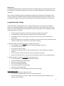
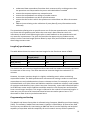
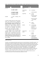
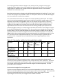
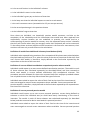
Response rates
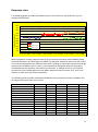
The following graph provides household response for waves one, two and three, by the
monthly field periods.
WAS - household response rates
100%
90%
80%
cooperating households
70%
60%
50%
40%
w1
30%
w2
wave 3 - old
20%
wave 3 - new
10%
July
Sep
Nov
Jan
Mar
May
Jul
Sep
Nov
Jan
Mar
May
Jul
Sep
Nov
Jan
Mar
May
Jul
Sep
Nov
Jan
Mar
May
Jul
Sep
Nov
Jan
Mar
May
Jul
Sep
Nov
Jan
Mar
May
0%
WAS achieved an average response rate of 55 per cent for wave one, with fieldwork being
conducted between July 2006 and June 2008. The achieved sample for wave one was issued
for re-interview between July 2008 and June 2010, yielding an improved response of average
response rate of 68 per cent. In wave 3, interviews were attempted with the responding
households and non-contacts from waves one and two. In addition to this a new random
sample of around 12,000 addresses was added. Response rates for these “old” and “new”
cohorts in wave three are shown separately.
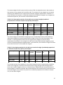
The following table provides a detailed breakdown of the outcome of cases included in the
set sample for both waves one and two.
Outcome
Issued cases
Eligible cases
Co-operating households
Non-contacts
Refusal to HQ
Refusal to interviewer
Total Refusal
Other non-response
Response rate
Non-contact
Refusal to HQ
Refusal to interviewer
Other non-response
Wave one
61917
55835
30511
3889
3805
15397
19202
1770
55%
7%
7%
28%
3%
Wave two
32195
29584
20009
2717
1268
4527
5795
1063
68%
9%
4%
15%
4%
Wave 3 old
25234
21397
15517
1503
809
2868
3677
700
73%
7%
4%
13%
3%
Wave 3 new
12683
11297
5734
988
876
3296
4172
403
51%
9%
8%
29%
4%
W3 all
37917
32694
21251
2491
1685
6164
7849
1103
65%
8%
5%
19%
3%
15
Keeping in Touch
WAS is a longitudinal survey that follows all adults interviewed in wave one (original sample
members, or OSMs). The survey is biennial, i.e. two years in-between each interview. WAS,
like other longitudinal surveys, experiences attrition, which may occur for inevitable reasons
such as death, or for reasons that can be minimised such as failure of tracing, failure of
contact, or refusal.2
The longitudinal design of WAS requires following OSMs over time in order to be able to
measure changes in wealth. It is evident that tracing and following sample members
becomes difficult when circumstances of sample members, in particular their location,
change over time.3 To minimise attrition caused by the loss of sample members due to the
failure of tracking, WAS has a number of measures implemented in the survey design to
maximise the likelihood of contact being made with the sample member at the next wave.
Firstly, the WAS questionnaire asks respondents at the interview to confirm their address
details as well as further contact details such as phone numbers, email address, and contact
details of two nominated persons (not resident at the same address) that are authorised to
provide ONS with the respondent’s new address in case the respondent has moved and
cannot be traced. Secondly, a few weeks after the interview all respondents receive a
‘Change of Address’ card together with the posted incentive (alternatively this will be sent
by email), which aims to encourage respondents to inform the ONS if their contact details
change. Thirdly, a brief telephone interview is conducted prior to the next wave’s interview.
This telephone interview is referred to as the ‘Keep in Touch Exercise’, or KITE. During this
interview information about household members as well as their address and contact details
are confirmed or updated. It provides the opportunity to identify movers from the
household, and their new contact details; as well to identify joiners to the household.
2
Portanti, M.: “Attrition on Longitudinal Survey – Literature Review”, ONS Working Paper, Social Survey Division, November
2009, pg. 2
Plewis, I., 2007. Non-Response in a Birth Cohort Study: The Case of the Millenium Cohort Study. International Journal of Social
Research Methodology, 10(5), p. 325
3
Laurie, H., Smith, R. & Scott, L., 1999. Strategies for Reducing Nonresponse in a Longitudinal Panel Survey. Journal of
Official Statistics, 15, p. 269
16
Questionnaire Content
Overview
The Wealth and Assets Survey (WAS) collects data on a wide range of assets and liabilities
that private individuals and households in Great Britain have. The primary aim of the survey
is to derive overall estimates of wealth and monitor how these change over time. WAS
broadly splits wealth into four categories:
1)
2)
3)
4)
Financial wealth
Pensions wealth
Physical wealth
Property wealth
The questionnaire is designed to collect relevant information across these four domains of
wealth, to provide aggregated measures of wealth, but also to afford significant potential for
analysis within these four domains. The questionnaire is therefore both broad and detailed
in coverage, with a wide range of stakeholders interested in the data WAS provides.
The wave one questionnaire content was determined by the requirements of the WAS
consortium of government departments at that time; namely the Department for Business
Innovation and Skills (BIS); Department for Work and Pensions (DWP); HM Revenues and
Customs (HMRC); HM Treasury (HMT), and; the Office for National Statistics (ONS); the
Department for Communities and Local Government (DCLG) and the Cabinet Office (CO) The
primary focus of the questionnaire is to provide for estimates of wealth; however some
additional information is collected on non-wealth topics such as socio-demographic
characteristics, income and financial acuity. This allows for aggregate and component
analysis of wealth with other factors.
Questionnaire changes
WAS is a longitudinal survey and therefore in order to measure change over time the
questionnaire needs to be as stable as possible; so as to reduce discontinuities in the
outputs. However, there is scope to make changes to the questionnaire between waves in
order to adopt harmonised question standards and/or emerging information requirements.
Changes between waves are made with consortium agreement. Sponsoring departments
provide their information requirements and specify any requested changes. These changes
are discussed by the WAS Technical Group (TG), with recommendations for questionnaire
changes being submitted to the WAS Steering Group (SG). The WAS SG is formed from senior
representatives of the consortium departments. Recommended questionnaire changes have
previously been subject to cognitive question testing and quantitative piloting. The cognitive
question testing has the following objectives:
 ascertain whether the proposed questioning will address the information needs
identified by key users and stakeholders, from the respondents’ perspective
 establish what respondents understand the questions to mean and the terminology
used
17






understand how respondents formulate their answers and by so doing ensure that
the questions are interpreted as key users and stakeholders intended
ensure that response options are comprehensive
ensure that respondents are willing to provide answers
ensure that respondents are able to provide answers
ensure that the order in which the questions are asked does not affect the answers
given
address issues relating to the collection of proxy data (if proxy information can be
collected)
The quantitative piloting aims to provide a test run of the new questionnaire, and to identify
any issues with the questionnaire before the next wave’s data collection starts. An
interviewer de-brief is held following the pilot to seek feedback on the questionnaire and
any areas for improvement. The pilot also provides the opportunity to produce survey
metrics such as interview length (broken down by topic area) and indicative response and
data linkage consent rates.
Length of questionnaire
The table below shows the mean interview lengths for the first three waves of WAS.
WAS wave
WAS (wave 1)
WAS (wave 2)
WAS (wave 3)
Mean interview
length (mins)*
88
85
75
75th percentile
90th percentile
103
104
91
135
137
119
The mean wave one interview length was 88 minutes and has remained relatively consistent
for wave two of the survey. The mean wave three interview length has reduced to 75
minutes.
However, the mean interview length is a slightly misleading metric when considering
respondent burden. The WAS questionnaire uses extensive routing in order to ensure that
respondents are only asked questions that are relevant to them. For example, a one adult
household with no or little assets and liabilities would be routed to a relatively small number
of questions and therefore have a short interview. Conversely, a two adult household with a
lot of different assets and/or liabilities would be routed to a lot of questions and therefore
have a much longer interview. This range is reflected in the variance of interview lengths. In
wave one, ten per cent of all interviews lasted at least two and a quarter hours. This
decreased in wave three to just below two hours.
Programming and testing
The Wealth and Assets Survey data is collected using Computer Aided Personal Interviewing
(CAPI). The software, loaded into interviewer’s laptops is called Blaise. All face to face ONS
social surveys use Blaise for interviewing as ONS feel that it has the flexibility and technical
capability to cope best with the complexity of social research surveys. Blaise's powerful
18
programming language offers numerous features and its data entry program supports a
variety of survey processing needs4.
A number of features of Blaise are particularly advantageous for this survey:

Blaise CAPI scripts have an in-built hierarchical block structure that effectively makes
all questionnaires modular. The ability to handle the associated routing of a modular
questionnaire is core to Blaise’s architecture. In addition to its hierarchical block
structure, Blaise also allows the creation of ‘blocks’ which can be accessed in parallel,
allowing interviewers to switch out of one set of hierarchical blocks to another set.
This provides valuable flexibility as it, for instance, allows an interviewer to pause an
interview with one household member, initiate an interview with another household
member (e.g. a household reference person), and then resume the interview with
the original household member at a convenient time in the future.

Blaise meets the requirement of being able to split the sample geographically or by
sample identifiers. Separate questions can be allocated to these different sections of
the sample or to randomly selected sub-samples of different sizes.

Handling complex routing (including loops and repeated events), applying automatic
logic and consistency checks in real time during the interview, and using text fills
where required, are all core to Blaise’s architecture. They are functions that we make
extensive use of on the Wealth and Assets Survey.
Blaise allows interviewers to exit and restart interviews at any point which allows interviews
to be suspended and resumed.
The Wealth and Assets Survey questionnaire records the length of time spent on different
questions during interviews, by placing ‘time stamps’ at the start and end of different
questions. We can use the session log file (called the audit trail in Blaise) to time individual
questions. This method affords us the ability to monitor how different questions contribute
to the overall length of the questionnaire, which is essential when conducting questionnaire
content reviews.
Other features of Blaise which make it excellent for undertaking the Wealth and Assets
Survey include:
4

the ability for interviewers to back track in instances where later sections of an
interview highlight an error made earlier

flexibility over styles, fonts, font sizes and colours. Blaise allows these to be specified
for all text or for individual words/questions etc. This helps ensure the screen seen by
the interviewer is as well designed as possible, with effective interviewer prompts.
This in turn helps promote interviewer-respondent rapport, thereby contributing to
better data quality
http://www.blaise.com/capabilities
19

the ability to interact with a ‘question by question’ (QbyQ) help facility. This provides
interviewers with real-time access to guidance on specific questions during the
interview. This is an electronic programme that operates in conjunction with Blaise
The Wealth and Assets Survey questionnaire is tested extensively prior to being scattered to
field interviewers. Currently, staff in the research team independently test the
questionnaire; along with staff in ONS Survey Operations team. Questionnaire testing is
done every month prior to the questionnaire scatter for the next fieldwork period.
20
Editing
An extensive range of computer edits were applied to both the household and individual
questionnaires during data entry in the field and to the aggregate data file in the office.
These edits checked that:





logical sequences in the questionnaire had been followed
all applicable questions had been answered
specific values lay within valid ranges
there were no contradictory responses
that relationships between items were within acceptable limits.
Edits were also designed to identify cases for which values, although not necessarily
erroneous, were sufficiently unusual or close to specified limits as to warrant further
examination.
Once an interview had taken place, the WAS data were transmitted back to ONS and were
aggregated into monthly files. Further editing occurred at this stage and included:




recoding text entries if an appropriate response category was available
investigating interviewer notes and utilising the information where applicable
confirming that overridden edit warnings had been done correctly
broad data consistency checks
The next stage involves checking that the routing of the questionnaire output is correct,
using a process referred to as ‘base checks’. SPSS programmes are run to emulate the
routing performed in Blaise. This process is used to identify where Blaise has incorrectly
routed respondents. This can either be corrected for by recoding data, or, where cases
haven’t been routed as they should have been; imputation requirements are specified.
Where errors in routing are discovered, the Blaise questionnaire is corrected to enhance the
quality of future data collection. The sooner base checks are performed; the sooner the
Blaise questionnaire can be corrected; thus leading to lower levels of data imputation.
Editing and validation processes for the second wave of WAS were similar to those used for
wave one: more details are provided in section 10.4 of the wave one report5. However, due
to the longitudinal component of the survey design, part of the achieved sample size in wave
two is linkable to wave one data. Therefore it was important to introduce longitudinal edit
checks to the existing editing and validation processes.
The edit and validation checks were run in two stages, whereby first cross-sectional checks
were carried out on the second wave to validate or edit outliers. As opposed to checks for
the property and physical wealth data, checks for financial and pension wealth data were
exclusively done on individual level because of the way the data had been collected. The
investigation of outliers largely focused on the top and bottom ten per cent of the
distribution of each wealth component, although for some variables this proportion was
reduced if the number of cases highlighted for investigation was particularly high. When
5
http://www.ons.gov.uk/ons/rel/was/wealth-in-great-britain/main-results-from-the-wealth-and-assets-survey2006-2008/report--wealth-in-great-britain-.pdf
21
outliers were investigated in the pensions or the financial section, various variables within
the same wealth component section or even different sections of the questionnaire were
included to establish whether particularly large outliers could be explained by the
circumstances of respondents. The majority of investigated cases proved to be genuine and
only a small number of cases had to be edited, whereby data was only edited if sufficient
information was recorded by interviewers to establish the correct response.
The second stage of checks was conducted after the linkage exercise was completed. At this
stage the change of wealth components between the two waves was calculated and
subsequently outliers of change were highlighted. To investigate these outliers, the
circumstances of relevant respondents in both waves had to be considered to decide
whether the value in either wave one or wave two was correct. As with the cross-sectional
checks only a small number of corrections were made for each wealth component variable
where sufficient information was available.
22
Imputation
General Methodology
In a way similar to all social surveys, data from the Wealth and Assets Survey contained
missing values. Users of WAS data need to distinguish between item non-response, which
typically occurs when a respondent does not know or refuses to answer a particular survey
question, and unit non-response: missing units where an individual in a responding
household refuses to be interviewed or a contact cannot be made. Item and unit nonresponse can be problematic in that many standard analytical techniques are not designed
to account for missing data. More significantly, missing data can lead to substantial bias and
inconsistencies in estimates and publication figures. Imputation is a statistical process that
serves to counter these problems by replacing missing values with valid, plausible data. To
avoid distorting the data through this process inappropriately the method applied must
account for the survey question structure and the distributional properties of the observable
data that structure yields. It must also take into account the possibility that unrecorded data
is not missing completely at random. It is important to note that as the overarching aim of
imputation is to improve the utility of the data, the key analytical aims of the survey should
also be factored into the design of the imputation process.
Information about discrete assets or liabilities recorded by the Wealth and Assets Survey
was collected through a relatively consistent question structure. Typically, an affirmative
response to routing questions designed to determine; do you have asset/liability x? was
followed by a question to specify the value; what is the amount/income/expenditure of
asset/liability x? In cases where an exact amount was not known, participants were asked to
provide a banded estimate from a range of bound values such as £0 to £100, £101 to £500,
and so on.
For imputation, the structure of the survey questions gives rise to several important
distributional properties in the data. Data from routing questions are categorical. Data from
amount/income/expenditure questions can be highly skewed. Furthermore, distributions are
often characterised by discrete steps or clustering. This can emerge through constraints
imposed by implicit laws or regulations governing the absolute value of an asset or liability,
or through respondents able only to provide a banded estimate. The key analytical aim of
the survey was to provide longitudinal estimates of change over time as well as crosssectional/single year estimates. To meet this aim the imputation must account not only for
the distributional properties of the data associated discretely with each variable, but also the
distributional properties of the rate of growth and/or decay over time.
At this point data users should be aware that the previously released wave one data only
included imputation for item non-response. Over the course of processing wave two data
the decision was made to also impute missing data from unit non-response to minimise the
underestimation of household wealth. In order to make data records comparable on
longitudinal level, all longitudinal records that were a unit non-response in wave one were
also imputed in the recent imputation exercise for the wave two report. However, this
means that when conducting cross-sectional analysis based on wave one data, only part of
the data was imputed for unit non-response.
23
In general, because of the distributional properties of the data elicited by the Wealth and
Assets question structure, missing data was best treated using a non-parametric imputation
method. To this end, all item non-response and unit non-response was imputed using a
Nearest-Neighbour approach (Bankier, Lachance, & Poirier, 1999; Durrent, 2005; Waal,
Pannekoek, & Schltus, 2011). In this approach, missing data was replaced with plausible
values drawn from other records in the data set referred to as ‘donors’. For categorical data
and skewed or clustered continuous data, donor-based methods are advantageous in that
they use only values actually observed in the data. Significantly, this helps to avoid the
distributional assumptions associated with parametric methods such as regression
modelling. Importantly, if applied correctly, imputation will estimate the distributional
properties of the complete data set accurately (Rubin, 1987; Chen & Shoa, 2000, Durrent,
2005).
Donor Selection
The key to a successful application of Nearest-Neighbour imputation is the selection of a
suitable donor. In general, donors were selected based on information specified by other
‘auxiliary’ variables in the data. Typically, auxiliary variables are employed to constrain
donor selection in two ways. Primarily, they serve to identify donors with similar
characteristics as the respondent with missing data. Importantly, the auxiliary variables
should be related with the data observed in the variable currently being imputed to help
estimate accurately the missing value. Auxiliary variables can also be applied to ensure
donor selection is tuned towards the key analytical aims of the survey and planned outputs.
For all imputed variables in the Wealth and Assets Survey, appropriate auxiliary variables
were identified through traditional regression-based modelling supplemented by guidance
from experts familiar, not only with a particular subject domain, but also with the analytical
program designed to provide outputs that meet customer needs.
Imputation was implemented in CANCEIS, a Nearest-Neighbour imputation tool designed
and developed by Statistics Canada (Cancies, 2009). The CANCEIS platform was configured to
select a suitable donor for each record needing treatment in two stages. In the first stage, a
pool of potential donors was established through two nested processes. The first process
divided all records in the survey into ‘imputation classes’ based on cross-classification of
auxiliary variables chosen for this stage. Potential donors could only be selected from the
sub-population of records in the same class as the record currently being imputed. The
second process served to refine the potential donor pool by ranking all of the records within
class. Ranking was determined by calculating the ‘distance’ between the potential donor and
the recipient record based on a second set of auxiliary variables referred to as matching
variables. Where appropriate, the calculation included differential weighting to account for
cases were some auxiliary variables were more important than others. In general, one of two
distance functions were used to calculate the distance between the potential donor and the
recipient record, depending on the characteristics of each particular auxiliary variable:the recipient record with auxiliary variables
the potential donor record with auxiliary variables
24
∑
the weight for the
variable
the individual distance for the
variable
For categorical data with no ordinal relationship between categories:-
(2)
{
For categorical or continuous data with an ordinal and/or ratio relationship between
categories or values:|
{
(
desired minimum(|
|
|
|
)
|) at which point and beyond
1
A subset of records with the smallest distance values were selected for the final potential
donor pool as these were most similar to the record being imputed. For non-categorical
data, extreme outliers were excluded from the donor pool to prevent propagation of values
likely to have a significant impact on estimates derived from the data. These were identified
through expert review and routinely represented values greater the 95 th percentile of the
observed data’s distribution. Table 1 shows a typical example of an auxiliary variable set.
This particular set was used to impute an unknown value for a respondent’s private pension.
All Wealth and Asset variables were treated in a similar way.
25
Table 1. Imputation Classes and Matching Variables used for imputing values for Private Pensions 1
Imputation Class
Matching Variable
Variable
Classification
Variable
ω Classification
Banded
1: Less than £2,500
Annual
Gross 0.3 Various amounts
Estimate
Salary
2: £2,500 > £4,999
3: £5,000 > £9,999
Employment
0.2 1: Employee
Status
4: £10,000 > £19,999
2: Self-Employed
5: £20,000 > £49,999
6: £50,000 > £99,999
Age Group
0.1 1: 16-24
7: £100,000 or more
2: 25-44
3: 45-59 (Female)
tSample
3 month sampling time
45-64 (Male)
frame
4: 60-74 (Female)
65-74 (Male)
To impute missing values for private pensions
5: 75+
donors were selected from an imputation
class derived from the cross-classification of
Sex
0.1 1: Male
observed Banded Estimates and tSample. The
2: Female
Banded Estimate provided an important
constraint on donor selection based on
NS-SEC
0.1 1: Professional
observed data. tSample was also significant
2: Intermediate
as research had indicated that private
3: Routine
pensions were particularly sensitive to
4: Never worked
economic trends over a short time frame.
5: Unclassified
The matching variable set consisted of
variables related to the observed data
Employment
0.1 1: Private
identified through modelling and domainSector
expert review. Annual Gross Salary and
2: Public
Employment status were given higher weights
3: Other
when calculating the distance between the
recipient record and the potential donor as
Education
0.1 1: Degree level
the strength of association was stronger for
2: Other level
these variables.
3: Level unknown
4: No qualifications
1
Applied only to cross-sectional data where the respondent was new to the survey and did not have observed
data for other waves.
Typically, the final potential donor pool was set to contain between 10 and 20 records. It is
important to note that through the first stage of constructing a potential donor pool, the
two nested processes used to establish this pool provide an implicit distributional model of
the frequency, range, and variance of the set of discrete values observed in the data for
records with characteristics similar the record being imputed. In the last stage of the
process the final donor was selected at random. Consequently, the probability of a
particular category or value being selected was proportional to the number of times that
category or value was observed with respect to the total number of observation. This
strategy served to support the aim of ensuring that the imputation did not have an
unwarranted impact on the distributional properties of data.
26
Processing Strategy
The Wealth and Assets Survey data were processed in three Sections: Property & Physical,
Pensions, and Financial. For all variables, imputation followed a basic processing strategy.
First, missing routing was imputed against an appropriate set of auxiliary variables. Following
that, where the routing indicated a missing value for the amount associated with a particular
asset/liability, the value was imputed against its own set of auxiliary variables. To meet the
key analytical aim of the survey; to provide longitudinal estimates of change over time as
well as cross-sectional/single year estimates, the detail of the basic processing strategy
varied for cross-sectional data belonging to respondents new to the survey, compared to the
longitudinal data belonging to respondents who had been in the survey for both Wave1 and
wave two.
In general, for respondents with cross sectional data only, processing focused on imputing a
discrete category or value drawn from the range and distribution of categories/values
observed directly in the data of records reaching the final potential donor pool. For these
respondents, donors were selected against a set of auxiliary variables in a way similar to
those outlined in Table 1. In contrast, for respondents with longitudinal data, the processing
strategy was tuned more towards the observable interdependencies and rates of change in
the data between wave one and wave two. To this end, when imputing each variable,
respondents with longitudinal data were divided into four imputation groups as outlined in
Table 2.
Table 2. Wave one and wave two longitudinal Imputation groups
Data Status
Wave one
Wave two
Imputation Group
Observed
Observed
Potential donor (O:O)
Missing
Missing
Missing both Waves (M:M)
Missing
Observed
Missing Wave1 (M:O)
Observed
Missing
Missing Wave2 (O:M)
For each variable, potential donors were selected only from records with valid observations
in both waves (O:O). When imputing values for respondents with data missing in both waves
(M:M), discrete values for both waves were drawn from a single donor. This strategy served
to preserve any implicit interdependencies between waves for categorical data and any
implicit rates of growth and/or decay for data with continuous characteristics.
To maintain the principle of the longitudinal processing strategy when imputing missing data
in records where data was observed in one wave but missing in the other (M:O or O:M)
categorical data was treated slightly differently than continuous data. For categorical data, a
discrete value observed in one wave was employed to serve as a constraint on donor
selection in the same way as an imputation class when imputing the missing value in the
other wave. For continuous data, an appropriately banded range was used in a similar way.
However, instead of taking a discrete value from the donor, the ratio that described the rate
of growth or decay in the donor between waves was transferred to the record to be
imputed. The ratio was then used in conjunction with the observed value in one wave to
calculate missing value in the other. This strategy is typically referred to as ratio-based rollback (M:O) or roll-forward (O:M) imputation. Table 3 shows a typical example of a
longitudinal auxiliary variable set used to impute a missing value for a respondent’s private
27
pension in Wave2 in the presence of observable data in wave one. Comparing Table 3 and
Table 1 will help identify the subtle differences between cross-sectional and longitudinal
imputation processing strategies.
28
Table 3. Imputation Classes and Matching Variables used for the longitudinal imputation of Private
Pensions in wave two in the presence of observed data in wave two
Imputation Class
Matching Variable
Variable
Classification
Variable
ω Classification
Banded Value
1: Less than £2,500
Annual
Gross 0.3 Various amounts
Salary
observed in
2: £2,500 > £4,999
Wave1 & Wave2
Wave1
3: £5,000 > £9,999
4: £10,000 > £19,999
Employment
0.2 1: Employee
Status
5: £20,000 > £49,999
Wave1 & Wave2
2: Self-Employed
6: £50,000 > £99,999
7: £100,000 or more
Age Group
0.1 1: 16-24
8: No Pension in Wave1
Wave2
2: 25-44
3: 45-59 (Female)
Banded
1: Less than £2,500
45-64 (Male)
Estimate
Wave2
2: £2,500 > £4,999
4: 59-74 (Female)
3: £5,000 > £9,999
65-74 (Male)
4: £10,000 > £19,999
5: 75+
5: £20,000 > £49,999
6: £50,000 > £99,999
Sex
0.1 1: Male
7: £100,000 or more
Wave2
2: Female
tSample
Wave1
Wave2
3 month
frame
sampling
time
&
To impute missing data in wave two based on
rates of growth/decay between waves, donors
were selected with reference points in wave
one similar to the recipient record based on an
imputation class derived from the crossclassification of observed Banded Values in
wave one, observed Banded Estimates in wave
two, and tSample in both waves. The category
‘No Pe sio i wave o e’ helped differe tiate
between new and established pensions.
Topic expert review also indicated that
changes in Gross Salary and Employment
Status were likely to contribute to the variance
in rates of change between waves.
Consequently wave one and wave two data for
these variables were included in the donor
selection process.
NS-SEC
1: Professional
Wave2
2: Intermediate
3: Routine
4: Never worked
5: Unclassified
Employment Sector
Wave2
0.1
1: Private
2: Public
3: Other
Education
Wave2
0.1
1:
2:
3:
4:
Degree level
Other level
Level unknown
No qualifications
Other notable variations in the processing strategy applied to the Wealth and Assets data
described to this point were associated typically with samples too small to implement
imputation classes based on complex multivariate cross-classification. In such cases,
variables that would have been included in donor selection as an imputation class were
included instead as a matching variable. Accordingly, the weights applied to the matching
variables were adjusted to best suit a preferred priority order. In extreme cases, where for
29
instance, a variable contained less than twenty observations and a small number of missing
values, imputation was based on deterministic editing. The range and variance of values
imputed this way was guided by topic expert review and was often based on the mean,
median, or mode of the observable data.
Quality Assurance and Evaluation
Without exception, the imputed data for all Wealth and Asset variables was examined and
tested before being formally accepted. The overarching aim of each evaluation was to
ensure that the distributional properties of the observed data had not been distorted
inappropriately by the imputation process. Fundamentally, evaluation was based on a
comparing the observed data prior to imputation with the fully imputed data. In all cases,
any notable departures from the observed data based on statistical measures such as shifts
in central tendency or variance and/or the introduction of unexpected changes in the shape
of the distribution had to be justified. Justification was based on the identification of subpopulations in the data with proportionally higher non-response rates that would
correspond with an appropriate observable change in the properties of the data. This
preliminary evaluation was supplemented by a more detailed review of the utility of the data
by topic experts familiar, not only with the analytical aims of the survey, but also with
expected data trends and characteristics inferred from other reliable external data sources.
30
Weighting
Overview
The weighting strategy embeds two important principles. The first principle is to maintain
the link between the initial selection probability and the ongoing loss to follow up (LTFU)
adjustments that remain for the evolving respondent subset over time. This is achieved
through developing the longitudinal base-weight from the wave one cross-sectional weight.
The second principle is that SSMs in the survey receive a temporary share of the base weight
appropriate to their status at any given time point. These principles enable the weighting to
refer back to the desired populations as closely as is possible with the current design.
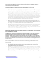
Terminology
As the survey develops, there are numerous combinations of responding patterns e.g.
responded in all waves, or responded in the first and second wave but not the third etc. The
number of categories is extended further when the wave in which the participant was
sampled is considered as well as the wave in which the participant first responded, and
whether respondents are original sample members (OSMs) or SSMs. These different
categories are treated differently throughout the weighting process and so it is necessary to
categorise individuals before weighting. A variable called ‘sumstat’ has been created to
identify the different categories (see table 2.1). The classification of each sumstat is included
which describes the sampling and responding behaviour of individuals in each sumstat. This
includes terms such as:
OSM – an Original Sample Member which refers to an individual who was sampled and who
responded in the first wave.
EOSM – an Entrant Original Sample Member which refers to an individual who lives at an
address which was sampled in the first wave but the household did not respond until a later
wave.
SSM – a Secondary Sample Member which refers to an individual who joined a previously
responding household.
Sumstat Wave 1 Wave 2 Wave 3 Classification
0
Non-productive
1
OSM, not in W2 or W3
2
W2 EOSM, not in W3
3
W2 SSM, not in W3
4
W3 EOSM
5
W3 SSM
6
W3 new cohort
7
OSM, not in W3
8
W2 EOSM
9
W2 SSM
10
OSM, not in W2
11
OSM, W1-W3 survivor
Table 2.1: Categories of key subsets of respondents
31
Different Types of Weights
Along with the numerous combinations of responding patterns, as the survey develops there
are also numerous longitudinal weights that could be calculated from the many different
combinations of the waves. It would not be appropriate to calculate all possible sets of
weights and we have considered how to make the number of weights we calculate
manageable. Additionally, limiting the number of weights produced minimises the chance of
the weights being used incorrectly. We sought to choose those weights which will be most
useful to users. We propose, from W3 onwards, to produce three types of weights
calculated at each wave; these are as follows:
longitudinal weight for the survivors from wave 1 to wave T
longitudinal weight from wave (T-1) to wave T
cross-sectional weight for wave T
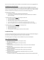
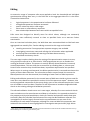
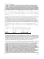
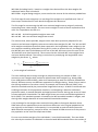
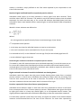
Figure 3.1 indicates the types of respondents which are included in each of the weighting
strategies at W3.
Wave 1
Wave 2
Wave 3
OSM
OSM
SSM (W2)
EOSM (W2)
OSM
SSM (W2)
EOSM (W2)
SSM (W3)
EOSM (W3)
New panel (W3)
KEY:
OSM = Original sample member
SSM = Secondary sample member
EOSM = Entry original sample member
W=Wave
Figure 3.1: Constituent respondent groups in each of the three weighting procedures
At W3, the longitudinal weight for the survivors consists of responders to all three waves, i.e.
W1, W2 and W3 (indicated by the red box in figure 3.1). The longitudinal weight for the
latest two consecutive waves is applied to all responders in W2 and W3 (demonstrated by
the purple box in figure 3.1). This includes OSMs from W1, as well as SSMs and EOSMs from
W2. Finally, the cross-sectional weight incorporates all responders to W3 (demonstrated by
the green box in figure 3.1). This consists of OSMs from W1, SSMs and EOSMs from W2,
SSMs and EOSMs from W3, as well as the new panel introduced in W3.
Longitudinal Weights
The weighting strategy is based on a principle of maintaining the link between the initial
selection probability and the ongoing loss-to-follow-up adjustments that remain for the
evolving respondent subset over time. This is achieved through developing the longitudinal
base weight (see e.g. Verma et al. 2007). This principle enables the weights to refer back to
32
the desired population as closely as is possible with the current sample design and
respondent follow-up procedures.
Different longitudinal base weights are used to construct the two longitudinal weights. The
product of the relevant W2 weight and the W3 attrition weights creates the W3 longitudinal
base weight. The relevant W2 weight is different for the two longitudinal weights, it is 1) the
longitudinal weight for the survivors, and 2) the W2 cross-sectional weight for the (T-1) to T
cases (as cases that do not appear in W1 do not have a W2 longitudinal weight).
(Construction of the W2 weights is detailed in Ashworth et al, 2012).
The first step in the weighting process is to develop the attrition models for W3. Two
separate steps were used to adjust for attrition:
a model for unknown eligibility status6
a model for non-response/non-contact
In both cases logistic regression7 was used to predict follow-up propensity, first for known
eligibility status and second for a response. This gives us an estimated propensity for each
case denoted by ˆ . Generically, i.e. ignoring subscripting, this is calculated as:
exp(βˆ T x)
1. ˆ 
1  exp(βˆ T x)
where βˆ is a vector of coefficients estimated by the regression model, and
response predictors in the regression model.
x
is a vector of
The first model predicted the log-odds of known to unknown eligibility status, using a set of
characteristics taken from the W2 survey data and using the W2 weight in the analysis. In
many cases, both respondents and non-respondents to W3 have data from W2, so a rich set
of response predictors is available. The ‘unknown eligibility status’ weights were calculated
as follows:
1
o
o
2. w3i  ˆ o , i  s3

i
where ˆio is the predicted probability that eligibility status at W3 is known, from the logit
model regressing eligibility status on various W2 individual and household level
o
characteristics for person i. s3 is the sample of people who have a known eligibility status at
W3. This is those who are 1) W1-W3 longitudinal cases for the survivor weights or 2) W2-W3
longitudinal cases for the (T-1) to T weights. These are the cases which are weighted up to
represent the cases with an unknown eligibility status at W3.
This often, but not exclusively, occurs when interviewers are unable to trace people who have moved
address (either whole households or household splits), as it is not known whether they remain in the
target population or not.
7 The regression model accounts for the clustered survey design with the nesting of observations (people
within households, households within PSUs) using the PSU as the ultimate cluster for the purposes of
calculating standard errors of coefficients.
6
33
In equation (3) below, ˆir represents the predicted probability of response from the known
eligibility status sample base, again using a logit model with W2 individual and household
level characteristics as predictor variables.
1
nr
w

, i  s3r
3
i
3.
r
ˆ
i
r
s3 is the sample of individuals within a responding household at W3, this is those who are 1)
W1-W3 longitudinal cases for the survivor weights or 2) W2-W3 longitudinal cases for the (T1) to T weights. These are the people who are weighted up to represent the nonrespondents at W3.
For individuals in a respondent household at 1) both W2 and W3 (for the (T-1) to T weights)
long
or 2) W1, W2 and W3 (for the survivor weights), the longitudinal base weight ( w3i ) is the
cal
product of the W2 weight ( w2 i ) and the two loss to follow up adjustment weights. For
long
individuals known to be part of movements out of the target population at W3 ( Out 3 ), w3i
cal
is the product of w2 i and the ‘unknown eligibility status’ weight:
4.
w3long
i
 w2cali w3oi w3nri ,
  cal o
w2i w3i ,


loss to population at W3 

i  s3r ,
longitudinal responders
i  Out 3,
long
The base weight w3i is trimmed at the 99th percentile, and scaled to the W2 population
total for the (T-1) to T weights and the W1 population total for the survivor weights.
The two longitudinal sub-samples (eligible respondents and ineligible outflows) are, after
adjustment for attrition, representative of the populations to which they relate back to (W2
for the (T-1) to T cases and W1 for the survivors), so it is possible to calibrate the longitudinal
base weight to the relevant population totals. This procedure should have the advantage of
making a further correction for any attrition not already accounted for, by adjusting the
weights to calibration control groups.
The calibration weights are calculated to sum to a set of known calibration totals t,
minimising the distance between the pre-calibration weight ( w3long
i ) and the calibrated
weight (which we write as an adjustment of the pre-calibration weight, gi w3long
). If the
i
membership of the calibration groups is represented by a vector of auxiliary values xi , then
the problem can be represented as:
5. min
 dist (w
long
3i
i
, gi w3long
such that
i )
x
3i
gi w3long
t
i
i
34
The final longitudinal calibration weight is the product of the g-weight and the initial
longitudinal base weight, where the g-weights are defined as the solution to (5). The gweight helps to rebalance the sample towards the population values of the variables
included in the calibration model.
Basic descriptive statistics relating to the W3 longitudinal weights for both the (T-1) to T and
survivor sub-samples are provided in Table 4.1. Descriptive statistics for the W1-W2 weights
are also provided for comparison purposes.
It is clear that due to attrition the sample size has decreased from W2 to W3. The sample
size for the survivor group (who were present in W1, W2 and W3) is smaller again, as this is a
subsample of the W2-W3 longitudinal cases. As the sample sizes get smaller, the mean
weight increases as each individual represents a larger proportion of the population. The
variation of the weights has increased since last wave as the weights have been further
adjusted to account for more characteristics of the evolving sample (non-response and
unknown eligibility status). It is interesting to note that the variation in the weights is higher
for the W2-W3 longitudinal cases than it is for the survivors even though the survivors are a
smaller subset. This has occurred because the minimum weight is smaller for the W2-W3
population whilst the maximum weights are the same for both subsamples. The maximum
weight reflects the trimming and the constraints imposed in the calibration process (i.e. the
99th percentile of the unadjusted distribution). The minimum weight is greatest for the
survivors, which is expected as each individual counts for a larger proportion of the
population.
Table 4.1: Descriptive statistics for the longitudinal weights
Weight
n
Mea Standar Coefficien Minimu
n
d
t of
m
deviati variation
on
W1-W2
43,338 1,341 642
47.9
203
longitudinal
W1-W2-W3
28,696 2,026 1,208
59.6
267
longitudinal
W2 - W3
31,472 1,870 1,236
66.1
155
longitudinal
Maximu
m
3,900
7,000
7,000
Cross-sectional Weights
A W3 pseudo cross-sectional weight has been created; pseudo because the data used
contains any W3 respondent regardless of the sample that they were selected in. Therefore
some of the sample (that were selected in W1) is not representative of the W3 population.
The original panel and the new panel have had weights calculated separately. The two
panels were then combined.
Cross-sectional weights for the original panel
There are several subgroups within the cross-sectional population and so there were many
different methods implemented when producing the cross-sectional weights. Those who had
previously responded had their most recent weight as their base weight. For cases
responding for the first time, the weights were created as follows:
35
W3 SSMs (including births) - based on a weight share derived from the base weights for
individuals within their household.
W3 EOSMs - original design weights, constructed as the inverse of the selection probabilities.
The final stage for each subgroup is a rescaling of the weights to a specified total. Each of
these steps are described in more detail throughout this document.
The first stage for constructing the W3 cross-sectional weight was to assign all previously
responding cases a base weight. The most recent weight for each of these respondents was
used. For respondents who were in:
W2 and W3 - W2-W3 longitudinal weights were used
W1 and W3 - W1 cross-sectional weights were used
This ensures that, where possible, weights which have been previously adjusted for nonresponse and unknown eligibility status were used as base weights for W3. The ‘W1 and W3’
cases weights would have previously been captured in the longitudinal cases weights by the
non-response modelling undertaken during W2. In order to account for this, the weights for
the W2-W3 cases were scaled down to the sum of the W2-W3 cases minus the sum of the
‘W1 and W3’ cases (see formula 6). This ensures that the ‘W1 and W3’ cases weights have
not been double counted. The scaling is carried out by multiplying the longitudinal cases
weights by the factor  rs1 where:
6.  rs1  
wi'W 2W 3cases '   wi'W 1andW 3cases '
w
i'W 2W 3cases '
wi is the weight of individual i.
The next challenge was to assign a weight to people entering the sample as SSMs. It is
common to use a weight share method to approximate these weights (e.g. Huang 1984,
Ernst 1989, Kalton & Brick 1995), rather than attempting to work out selection probabilities
directly. Different surveys use different approaches to weight sharing. Some surveys restrict
the sharing to adults or use other criteria, for example see Schonlau & Kroh (2010), who
detail the methods used by key international longitudinal surveys. As WAS is concerned with
enabling estimation for all population members, and weighting is based on calibrated
population totals, it seemed desirable and appropriate to ensure sharing was across all cases
enumerated within households. The WAS weight share was constructed following Kalton &
Brick (1995). This standard approach is based on the W2 household member’s weights, and
sharing these weights between all associated W3 household members.
A key challenge for the weight share method is being able to distinguish between those
SSMs who are new population entrants and those who were in the original population but
not originally in the sample. Unfortunately it is not possible to make this distinction with
WAS data and consequently, except for births, we treated all SSM entrants as if they were in
the population at the time the sample was drawn.
First we sum the base weights of the individuals i, in each W2 household j. Then we divide
this value by the number of individuals in the associated W3 household minus the number of
36
i
births, as shown in formula 7, where bwij is the base weight and N j is the number of
individuals in household j:.
N
i
j
 bw
ij
7. wij 
i j 1
N ij  births j
This ensures that all respondents within a household have a weight but that the sum of the
weights does not increase when SSMs (excluding births) enter the sample8. On the other
hand, a birth - either to an OSM or an SSM - is a true increase in the population and so, in
this case, the sum of the weights does increase. This method also holds when households
split between interviews. The sum of the W2 weights within a W2 household are shared
across the two associated W3 households. Finally the weights are scaled to the W3
population total (Nw3) using the scaling factor  rs 2 where:
8.  rs 2 
w
NW 3
i'W 2 W 3cases ','W 1andW 3cases '
The weight share allows longitudinal OSMs and SSMs to be treated together as a single subsample, but the construction of the original panel cross-sectional weight requires an
amalgamation of this sub-sample with EOSMs.
The EOSMs weights are their original design weights, constructed as the inverse of the
selection probabilities. These are then rescaled to the proportion of the responding W1
sample that they represent, multiplied by the W1 population total. Therefore the weights
were multiplied by the factor  rs 3 where:
9.  rs 3
 nEOSM 

  NW 1
nW 1respondents 


 wiEOSM
nEOSM is the number of EOSMs at W3, nW 1respondents is the number of W1 respondents, NW 1 is the
W1 population total and wi is the weight of individual i.
This subsample then needs to be combined with the weights for the OSMs and SSMs. The
EOSM’s weight would have previously been captured in the weights of the OSMs at W1
during the non response adjustments. In order to account for this, the weights for the OSMs
and SSMs were scaled to the W3 population total minus the sum of the EOSMs weights (see
formula 10). This ensures that the EOSM’s weights have not been double counted. In other
words, the OSM and SSM base weights were multiplied by the factor  rs 4 where:
This is a consequence of the assumption that population entrants were in the original
sample, which we made because the data do not allow us to distinguish population entrants.
8
37
10.  rs 4 
NW 3   wiEOSM
w
iOSM
  wiSSM
NW 3 is the W3 population total and wi is the weight of individual i.
Cross-sectional weights for the new panel
The new panel have design weights. This is the reciprocal of the selection probability of an
address. As there is oversampling of wealthier households, this needs to be incorporated
into the design weight construction.
The primary sampling units (PSUs) were sampled using a standard probability proportional
to size method, where the size is measured as the number of addresses9 per PSU. Within
each PSU, those addresses flagged as being from the predicted high wealth stratum were
sampled at 3 times the rate of other addresses in the predicted low wealth stratum.
The address selection probabilities for addresses from the ith PSU are thus:
P(address sampled )  P( PSU sampled ).P(address sampled | PSU sampled )
11.

nNi
.P(address sampled | PSU sampled )
N
where n is the number of sampled PSUs (324), Ni is the number of addresses in the this PSU
and N the total number of addresses included on the sampling frame in Great Britain.
For an address in the predicted high or low wealth stratum, respectively, the selection
probabilities are:
12. P(high stratum address) 
13. P(low stratum address) 
nNi
3  nPSU
. lo
N M i  2.5  M ihi
nNi
n
. lo PSU
N M i  2.5  M ihi
where nPSU is the number of addresses selected from each PSU (26 in year 1 and 13 in year
2), M ilo and M ihi are the number of addresses in the low and high stratum, in the ith PSU.
The design weights for the sampled addresses are then the reciprocal of the appropriate
address selection probability.
Once the new panel have design weights, a non response adjustment was applied. Non
response can bias the estimates if not accounted for; therefore responders are weighted up
to represent the non-respondents from the new panel sample. This was carried out in a
similar way to the attrition modelling in the longitudinal weights. A logistic regression model
was used to produce the response propensity for each case denoted by ˆir (see formula 1).
The adjusted weights for the new panel were calculated as:
The term address is taken here to refer to the delivery point as listed on the Postcode
Address File sampling frame.
9
38
wi  wi 
nr
14.
1
r
ˆ
i
where ˆir represents the predicted probability of response from the new panel using a logit
model with region, output area classification and quarter interviewed as predictor variables
and wi is the design weight.
Calibrating the cross-sectional weights
Once all cases in both panels have a weight, it is necessary to calibrate the cross-sectional
weights to population totals at W3. As the sampling design was different for the two years in
the new panel, these were also considered as two separate samples to reduce the variance
of the weights. Therefore calibration was carried out three times, once for the original panel,
once for year one of the new panel and once for year two of the new panel.
The aim of the cross-sectional weights is to create a single weight to cover both households
and individuals. In order to achieve this aim an ‘integrative calibration’ (Lemaître & Dufour,
1987) approach was used simultaneously to create both household and person level W3
pseudo cross-sectional weights. This results in all people in the household having the same
weight, which is also the household weight. The population totals to which the weights were
calibrated were based on interpolations of ONS’ mid-year estimates taken from the midpoint
of the W3 fieldwork period (June 2011).
The result at this stage is three sets of cross-sectional weights, each calibrated to the W3
population totals; one for the original panel and one for each year of the new panel. As users
will want to carry out analysis on the cross section as a whole, it is necessary to combine
these three sets of weights.
Combining the cross-sectional weights
In order to do this, the constructed weights for individuals in the original and new panels
were re-scaled in 2 ways:
in proportion to the achieved sample size for the three panels.
in proportion to the effective sample size for the three panels (as proposed by Chu et al
1999, Korn and Graubard 1999).
as
In the first option, the constructed weights were multiplied by the factors  orig
for the
as
as
original panel and  newy
1 and  newy 2 for the new panel where:
as
15. orig 
norig
norig  nnewy1  nnewy 2
as
 newy
2 
as
 newy
1 
nnewy1
norig  nnewy1  nnewy 2
nnewy 2
norig  nnewy1  nnewy 2
39
norig is the sample size of the original panel, nnewy1 is the sample size of year 1 of the new
panel and nnewy 2 is the sample size of year 2 of the new panel.
This scaling approach will result in each panels weights being in the same proportion to each
panels sample size. The weights were then re-scaled to the W3 population total by
multiplying by  rs 5 where:
16.  rs 5 
NW 3
 wi
The second option accounts for the variance within each panel and combines the weights
such that the variance is minimised. As the new panel is more representative of the W3
population (as it was selected more recently), and the weights are less variable (as they have
had fewer adjustments made to them), there is a potential improvement that could be made
by combining the weights in proportion to effective achieved sample sizes for the three
panels. For this method, firstly the design effect for each panel was calculated. The sample
size was then divided by the design effect to create the effective sample size. The three
panels were then combined proportional to their effective sample size by multiplying by the
es
es
es
factors  orig
for the original panel and  newy
and  newy
2 for the new panel where:
1
17. 
es
orig

eff
norig

norig  nnewy1  nnewy 2
eff
eff
eff

es
newy 2

es
newy 1

neff
newy1
eff
norig  nnewy1  nnewy
2
eff
eff
eff
nnewy
2
eff
eff
eff
norig
 nnewy
 nnewy
1
2
As this method gives more weight to those panels with a smaller variance, the new panel
have more power and the old panel slightly less. This process results in the sum of the
weights changing quite dramatically. Therefore the weights are calibrated a final time.
Descriptive statistics for the resulting weights are given in Table 5.4.1 (as for achieved
sample size and es for effective sample size). The equivalent statistics for the W2 crosssectional weights are also provided for comparison purposes. Table 5.4.2 and table 5.4.3
contain descriptive statistics of the weights broken down by key subsamples of the
population when the panels were combined in proportion to achieved sample size and
combined proportional to achieved sample size, respectively.
Table 5.4.1: Descriptive statistics for the W3 cross-sectional weight
Weight n
Mean Standard Coefficient Minimum Maximum
deviatio of variation
n
W2
46,347 1,277 730
57.2
106
3,700
W3(as) 49,447 1,207 963
79.8
74
9,999
W3(es) 49,447 1,207 877
72.7
69
9,999
40
The mean weight for W3 is quite similar to that of W2; the slight decrease is due mostly to
the increase in the sample size from W2 to W3. The variation in the weights has increased
reflecting the additional non-response and unknown eligibility adjustments. However it is
clear that when the sample is combined proportional to effective sample size, as appose to
achieved sample size, the variation is decreased as desired.
Table 5.4.2: Descriptive statistics for the W3 cross-sectional weight (combined
proportional to achieved sample size) split by sub-samples
Sub-sample
n
Mean
All cases
Longitudinal cases
W3 SSMs
W3 EOSMs
New panel
49,447
32,485
1,697
1,420
13,845
1,207
1,436
1,391
669
700
Standard
deviatio
n
963
1,067
1,177
178
233
Coefficient
of variation
Minimu
m
Maximu
m
79.8
74.3
84.6
26.7
33.3
74
74
74
205
149
9,999
9,999
9,999
1,302
1,908
The mean weights of the different subgroups vary considerably because of the different
adjustments applied to certain groups and the length of time the cases have been in the
sample. i.e. the longitudinal cases have the largest mean weights as most of these
respondents have been in the sample since W1 and so have had unknown eligibility status
and non-response adjustment applied twice. In line with this, the variation is larger for those
cases who have been in the sample the longest.
Table 5.3: Descriptive statistics for the W3 cross-sectional weight (combined proportional
to effective sample size) split by sub-samples
Sub-sample
n
Mean
All cases
Longitudinal cases
W3 SSMs
W3 EOSMs
New panel
49,447
32,485
1,697
1,420
13,845
1,207
1,339
1,300
619
945
Standard
deviatio
n
877
1,001
1,108
167
317
Coefficient
of variation
Minimu
m
Maximu
m
72.7
74.7
85.2
26.9
33.5
69
69
69
187
204
9,999
9,999
9,999
1,212
2,598
The second version of the weights is very similar especially when comparing the variability
within each subgroup. However the new panel have larger weights and the longitudinal
cases have smaller weights, which is an improvement. Additionally the overall variance of
these weights is smaller as desired. We recommend that the second version of the W3 crosssectional weights, those where the panels are combined proportional to effective sample
size, are the best weights.
41
Additional Considerations
The weighting process for future waves should be very similar to that used for W3. It will
therefore be important to analyse the additional considerations discussed below, such that
suitable recommendations can be made, and the most efficient weighting strategies can be
developed and taken forward for future waves.
A methodological change was made between W2 and W3. In W2, births to OSMs were given
their mother’s weight, rather than simply having their weight allocated through the weight
share. In W3, this has not yet been carried out due to time constraints. Further planned
work involves recalculating the cross-sectional weights using the W2 method and analysing
the impact on the weights. We believe that the impact will be relatively small, as it is unlikely
that the mother’s weight will vary much from the household average. Depending on the
results, we will conclude that either:
1) the impact on the weights is negligible, and does not warrant making changes to the
existing W3 weights
or
2) the impact on the weights is substantial, so the existing W3 weights will be updated
accordingly
The conclusion will also form the basis of a recommendation on the method to be used for
all future waves.
Typically pre-calibrated weights were carried forward from the previous waves during the
weighting strategies described above. It would be desirable to carry out further analysis in
order to quantify the differences between the final W3 weights produced using precalibrated and calibrated W2 weights to see if there is a significant difference.
The principle aim of WAS is the estimation of gross change, but it is also important to
produce cross-sectional estimates of wealth over time which, in turn, enables the
computation of net change. ONS will produce weights for each new release of data arising
from each completed survey wave to assist both longitudinal and cross-sectional analysis.
WAS weights are (model assisted) design-based weights. Users can re-scale and normalise, if
they so wish, in order to get the weights to sum to the sample size. However, the majority
of popular statistical packages available on the market now account more accurately for the
weights, so we recommend using survey-based procedures, where possible, when using
weights in the analysis of survey data. It is important to note that using the weights will help
to reduce bias. However, reducing bias comes at the cost of increasing variance of the
estimates. As the variance of the weights increases, so too does the estimated sampling
variance.
42
Data Quality
All reasonable attempts have been made to ensure that the data are as accurate as possible.
However, there are two potential sources of error which may affect the reliability of
estimates and for which no adequate adjustments can be made. These are known as
sampling and non-sampling errors and should be kept in mind when interpreting the WAS
results.
Sampling error
Sampling error refers to the difference between the results obtained from the sample
population and the results that would be obtained if the entire population were fully
enumerated. The estimates may therefore differ from the figures that would have been
produced if information had been collected for all households or individuals in Great Britain.
One measure of sampling variability is the standard error which shows the extent to which
the estimates should be expected to vary over repeated random sampling. In order to
estimate standard errors correctly, the complexity of the survey design needs to be
accounted for, as does the calibration of the weight to population totals (see Weighting).
WAS has a complex design in that it employs a two-stage, stratified sample of addresses with
oversampling of the wealthier addresses at the second stage and implicit stratification in the
selection of PSUs.
Although data users should produce standard errors with the outputs of their analysis, with
the WAS datasets available at UKDA this is not possible without design information (details
of weights, stratification, clustering and calibration). Such information could not be provided
with the datasets for statistical disclosure reasons. However, methodologists in ONS are
planning to develop and test the generation of appropriate standard errors.
Note that some initial estimates of standard errors for key variables are available in the
supporting tables to the report referred to above, but imputation effects need to be taken
account of, so these should be treated as preliminary: more accurate estimates would be
likely to be larger.
Non-sampling error
Additional inaccuracies, which are not related to sampling variability, may occur for reasons
such as errors in response and reporting. Inaccuracies of this kind are collectively referred to
as non-sampling errors and may occur in a sample survey or a census. The main sources of
non-sampling error are:



response errors such as misleading questions, interviewer bias or respondent
misreporting
bias due to non-response as the characteristics of non-responding persons may differ
from responding persons
data input errors or systematic mistakes in processing the data
Non-sampling errors are difficult to quantify in any collection. However, every effort was
made to minimise their impact through careful design and testing of the questionnaire,
training of interviewers and extensive editing and quality control procedures at all stages of
43
data processing. The ways in which these potential sources of error were minimised in WAS
are discussed below.
Response errors generally arise from deficiencies in questionnaire design and methodology
or in interviewing technique as well as through inaccurate reporting by the respondent.
Errors may be introduced by misleading or ambiguous questions, inadequate or inconsistent
definitions or terminology and by poor overall survey design. In order to minimise the
impact of these errors the questionnaire, accompanying documentation and processes were
thoroughly tested before being finalised for use in the first wave of WAS.
To improve the comparability of WAS statistics, harmonised concepts and definitions were
also used where available. Harmonised questions were designed to provide common
wordings and classifications to facilitate the analysis of data from different sources and have
been well tested on a variety of collection vehicles.
WAS is a relatively long and complex survey and reporting errors may also have been
introduced due to interviewer and/or respondent fatigue. While efforts were made to
minimise errors arising from deliberate misreporting by respondents some instances will
have inevitably occurred.
Lack of uniformity in interviewing standards can also result in non-sampling error, as can the
impression made upon respondents by personal characteristics of individual interviewers
such as age, sex, appearance and manner. In ONS, thorough training programmes, the
provision of detailed supporting documentation and regular supervision and checks of
interviewers' work are used to encourage consistent interviewing practices and maintain a
high level of accuracy.
One of the main sources of non-sampling error is non-response, which occurs when people
who were selected in the survey cannot or will not provide information or cannot be
contacted by interviewers. Non-response can be total or partial and can affect the reliability
of results and introduce a bias.
The magnitude of any bias depends upon the level of non-response and the extent of the
difference between the characteristics of those people who responded to the survey and
those who did not. It is not possible to accurately quantify the nature and extent of the
differences between respondents and non-respondents. However, the level of non-response
bias was mitigated through careful survey design and compensation during the weighting
process, the latter having been discussed earlier. To further reduce the level and impact of
item non-response resulting from missing values for key items in the questionnaire, ONS
undertook imputation (see Imputation).
Non-sampling errors may also occur between the initial data collection and final compilation
of statistics. These may be due to a failure to detect errors during editing or may be
introduced in the course of deriving variables, manipulating data or producing the weights.
To minimise the likelihood of these errors occurring a number of quality assurance processes
were employed which are outlined elsewhere in this guide.
External source validation
In the final stages of validating the WAS data, comparative checks were undertaken to
ensure that the survey estimates conformed to known or expected patterns and were
44
broadly consistent with data from other external sources. This work was undertaken by ONS
and analysts from the funding departments as well as a number of academics who had
expertise in the various topics included in WAS. The following guidelines were
recommended by ONS when undertaking the external source validation process:




identify alternate sources of comparable data
produce frequencies and cross tabulations to compare proportions in the WAS
dataset to those from external sources
if differences were found, assess whether these were significant
where significant differences were found ensure that reference periods, populations,
geography, samples, modes of collection, questions, concepts and derivations were
comparable
Results from these analyses indicated that estimates from the Wealth and Assets Survey
were broadly in line with results from other administrative and survey sources. Further work
to produce more detailed analyses and comparisons is ongoing and any data quality issues
which are identified with WAS variables will be fully documented and made available on the
ONS website.
45
Wealth estimates
The wealth estimates in this report are derived by adding up the value of different types of
asset owned by households, and subtracting any liabilities. Total wealth with pension wealth
is the sum of four components:




net property wealth;
physical wealth;
net financial wealth; and,
private pension wealth
Total wealth without pension wealth is the sum of the first three of these components.
The components are, in turn, made up of smaller building blocks:



net property wealth is the sum of all property values minus the value of all mortgages
and amounts owed as a result of equity release
physical wealth is the sum of the values of household contents, collectibles and
valuables, and vehicles (including personalised number plates)
net financial wealth is the sum of the values of formal and informal financial assets,
plus the value of certain assets held in the names of children, plus the value of
endowments purchased to repay mortgages, less the value of non-mortgage debt.
Some points to note:




informal financial assets exclude very small values (less than £250);
money held in Trusts, other than Child Trust Funds, is not included;
financial liabilities are the sum of current account overdrafts plus amounts owed on
credit cards, store cards, mail order, hire purchase and loans plus amounts owed in
arrears;
private pension wealth is the sum of the value of current occupational pension
wealth, retained rights in occupational pensions, current personal pension wealth,
retained rights in personal pensions, Additional Voluntary Contributions (AVCs), value
of pensions expected from former spouse or partner and value of pensions in
payment. Note that, while net property wealth, physical wealth and net financial
wealth are calculated simply by adding up the value of assets (minus liabilities, if
applicable) for every household in the dataset, private pension wealth is more
complicated because modelling is needed to calculate the value of current
occupational pension wealth, retained rights in occupational pensions etc for each
household. As with all models, the results depend on the assumptions made.
46
Private pension wealth measures
Nine separate components of private pension wealth were calculated based on the WAS
survey responses. There were four categories of pension to which respondents were making
(or could have made) contributions to at the time of the survey:




defined benefit (DB);
additional voluntary contributions (AVCs) to DB schemes;
employer-provided defined contribution (DC);
personal pensions
The distinction between employer-provided DC pensions and personal pensions is as
reported by the respondent. So, for example, if an individual had a Stakeholder Pension
facilitated by their employer and chose to report that as an ’employerprovided/occupational scheme’, this is counted as an employer-provided DC pension.
Conversely, if an individual reported this simply as a ‘Stakeholder Pension’, it would be
included in personal pensions.
In addition to these four categories of current pension scheme, wealth from five other types
of pension was calculated:





pensions already in receipt
retained rights in DB-type schemes
retained rights in DC-type schemes
pension funds from which the individual is taking income drawdown
pensions expected in future from a former spouse
How the wealth for each of these components was calculated is described in detail in the
following sections.
Current defined benefit occupational pension scheme wealth
Individuals could report up to two current defined benefit pensions. The wealth in each of
these schemes was calculated separately (as described below) and then summed to derive
total wealth in current defined benefit (DB) occupational schemes.
Wealth in these schemes was defined as:
Where:
AR is the age- and sex-specific annuity factor at normal pension age, R, based on (single life)
annuity rates quoted by the Financial Services Authority, assuming average age- and sexspecific life-expectancies (as estimated by the Government Actuary’s Department) and a
discount rate of 2.5 per cent.
YiP is annual pension income, defined as
47
αi is the accrual fraction in the individual’s scheme
ni is the individual’s tenure in the scheme
si is the individual’s gross pay at the time of interview
Li is the lump sum that the individual expects to receive at retirement
r is the real investment return (assumed to be 2.5 per cent per annum)
R is the normal pension age in the pension scheme
a is the individual’s age at interview
Since these are individual, not household, pension wealth measures, and due to the
complexity of the calculations and the information that would have been required from
respondents, survivor benefits are not modelled. In practice, this would lead to a
underreporting of pension wealth for women, since the expected future survivor’s benefits
that they will receive when they (on average) outlive their husbands will not be measured.
To the extent these survivors benefits will be sometime in the future for most women, their
omission will have only a small effect on the calculations.
Definition of wealth from Additional Voluntary Contributions (AVCs)
Individuals who reported being members of an occupational DB scheme were asked whether
they had made any AVCs and, if so, what the value at the time of interview of their AVC fund
was. Current AVC wealth is, therefore, simply defined as the fund value reported by the
respondent at the time of the interview.
Definition of current defined contribution occupational pension scheme wealth
Individuals could report up to two current defined contribution pensions. The wealth in each
of these schemes was calculated separately (as described below) and then summed to
derive total wealth in current defined contribution (DC) occupational schemes. This
procedure was also followed for those who reported that their employer-provided scheme
was a hybrid scheme or that they did not know the type of scheme.
Individuals were asked to report the value of their fund at the time of the interview and
were encouraged to consult recent statements where available. Current occupational DC
pension wealth is, therefore, simply defined as the fund value reported by the respondent at
the time of the interview.
Definition of current personal pension wealth
Individuals could report up to two current personal pensions; current being defined as
schemes to which the individual was (or could have been) contributing at the time of
interview. The wealth in each of these schemes was calculated separately (as described
below) and then summed to derive total wealth in personal pensions.
Individuals were asked to report the value of their fund at the time of the interview and
were encouraged to consult recent statements where available. Current personal pension
48
wealth is, therefore, simply defined as the fund value reported by the respondent at the
time of the interview.
Retained rights in defined benefit occupational pension scheme
Individuals could report up to three pensions in which rights have been retained. These
could be either DB of DC schemes. The wealth in each DB retained scheme was calculated
separately (in much the same way as for current DB schemes described above) and then
summed to derive total wealth held as retained rights in defined benefit (DB) occupational
schemes.
Wealth in these schemes was defined as:
Where:
AR is the age and sex-specific annuity factor at retirement age, R (see above)
YiP is expected annual pension
Li is the lump sum that the individual expects to receive at retirement
r is the real investment return (assumed to be 2.5 per cent a year)
R is assumed to be 65, or the individual’s current age if he/she was already aged over 65
a is the individual’s age at interview
Retained rights in defined contribution occupational pension scheme
The wealth in each DC retained scheme was calculated separately (in much the same way as
for current DC schemes described above) and then summed to derive total wealth held as
retained rights in DC schemes. Specifically, individuals were asked to report the value (at the
time of interview) of their retained DC fund.
Rights retained in schemes from which individuals are drawing down
Individuals could also report that they were already drawing down assets from a retained
pension scheme. In these cases, individuals were asked to report what the remaining fund
value for their scheme was at the time of interview. The wealth in each of these schemes
was then summed to derive total wealth held in schemes of this type.
Pensions expected in future from former spouse/partner
Individuals were asked to report in total how much they expected to receive in the future
from private pensions from a former spouse or partner. Respondents were given the choice
to report this either as a lump sum wealth figure, or as an expected annual income. Two
slightly different approaches were followed, depending on how the respondent answered.
For those who reported a total lump sum value, this figure was taken as the relevant wealth
measure and discounted back to the time of the interview. For those who reported an
49
expected future annual income, wealth was calculated in much the same way as for DB
schemes described above:
Where:
AR is the age- and sex-specific annuity factor at retirement age, R (see above)
YiP is expected annual pension
r is the real investment return (assumed to be 2.5 per cent a year)
R is assumed to be 65, or the individual’s current age if he/she was already aged over 65
a is the individual’s age at interview
Definition of wealth from pensions in payment
In order to calculate the value of the future stream of income provided by pensions from
which the individual was already receiving an income, the lump sum which the individual
would have needed at the time of interview to buy that future income stream from a
pension provider was calculated. Wealth from pensions in payment was therefore defined
as:
Where
Aa is the age- and sex-specific annuity factor based on respondent’s current age, a
YP is reported current annual private pension income
For those age groups for whom no market annuity factor was available (ages 75 and over),
we predicted a hypothetical annuity factor based on the information from those ages where
annuity prices were available
Contact details
For further information, or to provide feedback on the Wealth and Assets Survey
documentation, please contact Craig Orchard:
Phone: 01633 455755
Email: [email protected]
50