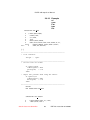
1
ESTEL-2D version v5p6
User Manual
JP Renaud
University of Bristol
December 4, 2006
Disclaimer
The information given in this manual is subject to revision without notice.
This manual is written for version v5p6 of the software.
It is necessary to have a basic knowledge of the Fortran programming language to use ESTEL-2D. This user manual is based on the assumption that
the user knows at least arrays, loops and tests in Fortran.
1
Chapter 1
Introduction
1.1
Typing conventions used in this manual
The keywords for the steering file are written in UPPER CASE BOLD.
All text which needs to be entered by the user either as Fortran code in
the Fortran file or as plain text in the various input files is written in monospace
font. The same font is also used to illustrate what is printed on screen or in
the output files.
Units are given in brackets with the following conventions: L for Length and
T is for Time. Therefore [L.T −1 S] is the dimension of a velocity.
The bibliographical references are indicated with a number in square brackets. The list of associated documentation is given in chapter ??.
ESTEL-2D is a two dimensional numerical model for water flow and solute
transport in porous media. It contains three modules: a flow module which
solves Richards equation in saturated and unsaturated porous media by the
finite element method, a particle tracking module which solves the advectiondispersion equation by the random walk method and a transport module which
solves the advection-dispersion, equation by the finite element or control volume finite element method.
1.2
1.2.1
Presentation of ESTEL-2D
Situation of ESTEL-2D in the TELEMAC system
The ESTEL-2D software is part of a complete set of computational software,
the TELEMAC system, which consists of the following modules:
MATISSE is used to build the grid of triangular elements,.
STBTEL software is used for reading the files produced by the mesh generators and creating a geometry file in the Selafin standard that can be read
by the simulation modules and by the RUBENS graphical post-processor.
STBTEL also carries out a number of mesh consistency checks.
2
ESTEL-2D v5p6 User Manual
TELEMAC-2D/3D carries out 2D hydrodynamic simulations and transport of
solute tracers.
TELEMAC-3D carries out 3D hydrodynamic simulations and transport of solute tracers.
SISYPHE software is used to simulate the transport of bed load.
ARTEMIS computes the transformation of wave characteristics in a coastal
area or harbour.
TOMAWAC is used to simulate the steady or transient sea state using a spectral method.
ESTEL-2D is used to simulate subsurface flows and solute transport in two
dimensions and is the object of this document.
ESTEL-3D is used to simulate subsurface flows in three dimensions.
POSTEL-3D produces 2D cuts inside the 3D results file of TELEMAC-3D or
SUBIEF-3D, in order to use the RUBENS graphical post-processor.
RUBENS is used for producing 2D graphical outputs of the results of the various simulation modules.
In addition to MATISSE, the TELEMAC system is interfaced with five commercial mesh generators:
1. IDEAS manufactured by SDRC
2. ICEM CFD manufactured by ANSYS
3. SIMAIL-2D manufactured by SIMULOG
4. TRIGRID developed by the Institute of Ocean Sciences, Canada
5. FASTTABS developed by the Engineering Computer Graphics Laboratory
of Brigham Young University, U.S.A.
6. ADCIRC developed by Notre Dame University, the University of North
Carolina and the U.S. Army Corps of Engineers
The simulation modules are written in FORTRAN-90, with no machinespecific language extensions. They can be run on all workstations operating
under Linux or Unix providing that a Fortran 90 compiler is available.
1.2.2
Computer environment
Users will have to use Fortran code to define some aspects of the simulation.
This is done in by using a number of so-called “user’s” subroutines, the source
code of which is provided with the system. The “user’s” subroutines are compiled at runtime and linked with the ESTEL-2D library.
Get the latest version online.
3
PDF file created on 4/12/2006
ESTEL-2D v5p6 User Manual
1.2.3
Programming by the user
The following procedure should be followed:
1. Recover the standard version of the user subroutine provided with the
system, and copy it into the working directory. A list of user subroutines
is given in chapter .
2. Modify the subroutines according to the model you wish to build.
3. Copy the set of subroutines into a single Fortran file that will be compiled
during the ESTEL-2D start procedure.
This procedure is described in more details in section .
Note that it is necessary to have a basic knowledge of the Fortran 90 programming language to use ESTEL-2D. This user manual is based on the assumption that the user knows at least:
declarations: integer, double precision, logical
arrays: myarray(i)
loops: do enddo
tests: if endif
subroutines/functions: mysubroutine(argument1,argument2)
Get the latest version online.
4
PDF file created on 4/12/2006
Chapter 2
List of input and output files
During a simulation, ESTEL-2D uses a number of input and output files, some
of which are optional.
2.1
2.1.1
Mandatory input files
The steering file
The steering file is an ASCII text file created by the user. It contains a number
of keywords to which values are assigned and used to “steer” the simulation.
The steering file is used to specify the names of the input and output files, the
type of simulation to run, the numerical parameters to use etc... The name of
the steering file is specified when running ESTEL-2D at the command line (see
).
An example of steering file is given in appendix and more information on
the syntax used in the steering file is given in appendix .
2.1.2
The geometry file
The geometry file is a binary file in serafin format []. It can be read by RUBENS
and is created either by MATISSE or by STBTEL using the file(s) produced by a
mesh generator. The geometry file contains all the information concerning the
mesh, i.e. the number of mesh points (NPOIN), the number of elements (NELEM),
coordinates of all the nodes in the mesh (X and Y) and also the connectivity table (IKLE).
Note that ESTEL-2D stores information on the geometry at the beginning
of the serafin results file. Because of this, the serafin results file can be used
as a geometry file if a new simulation is to be run on the same mesh.
The name of this file is given with the keyword: GEOMETRY FILE.
The boundary conditions file is an ASCII text file which complements the
geometry file. A boundary conditions file can be generated automatically by
5
ESTEL-2D v5p6 User Manual
MATISSE or STBTEL but note that the syntax used in ESTEL-2D is slightly different from the syntax of the other codes of the TELEMAC system (see section
). Therefore, editing might be necessary when using a boundary conditions
file with ESTEL-2D.
The
boundary
conditions
file
Each line of the file is dedicated to one point on the mesh boundary.
The file name is given with the keyword: BOUNDARY CONDITIONS FILE.
An example of boundary conditions file is given in appendix .
The soil database file is an ASCII text file created by the user. It describes
the hydraulic properties (permeability, porosity etc...) of each soil type used in
the simulation. A full description of the use of soil types in ESTEL-2D is given
in section .
The
soil
database
file
The file name is given with the keyword: SOIL DATABASE FILE
The Fortran file is an ASCII text file with the extension “.f” which is created
by the user. It contains both the ESTEL-2D subroutines modified by the user
and the subroutines that have been specially developed for the computation.
This file is compiled and linked to generate the executable program for the
simulation.
2.1.3
Optional
input
files
The
Fortran
file
The name of this file is given with the keyword: FORTRAN FILE.
An example of Fortran file is given in appendix .
The tracers definition file is an ASCII text file created by the user. It describes the transport properties (dispersion, diffusion etc...) of each tracer used
in the simulation either by the transport module or the particle module. A full
description of the use of tracers in ESTEL-2D is given in section .
Get the latest version online.
6
PDF file created on 4/12/2006
ESTEL-2D v5p6 User Manual
The
tracers
definition
file
The file name is given with the keyword: TRACERS DEFINITION FILE
An example of tracers definition file is given in appendix .
The source points file is an ASCII text file created by the user. It contains
the description of punctual injection of tracer (location, discharge, concentration
etc...). This is described in details in section .
The
source
points
file
The file name is given with the keyword: SOURCE POINTS FILE
An example of source points file is given in appendix .
The previous computation file is a binary file in serafin format. It is usually
the serafin results file of another simulation which will be read and used as
initial conditions for the current simulation. Therefore, the geometry contained
in this file needs to be identical to the one in the geometry file. A detailed
description of the use of a previous computation file is given in section .
The
previous
computation
file
The file name is given with the keyword: PREVIOUS COMPUTATION FILE
The reference file is a binary file in serafin format. It contains the results of
a previous simulation to which the current simulation will be compared. At the
end of the calculation, the result of the simulation can be compared to the last
time step stored in the reference file. The result of the comparison is given in
the control printout in the form of a maximum difference in pressure head.
The
reference
file
The name of this file is given with the keyword: REFERENCE FILE
Get the latest version online.
7
PDF file created on 4/12/2006
ESTEL-2D v5p6 User Manual
The serafin results file is a binary file in serafin format [06] in which ESTEL2D stores spatially distributed information during the computation. It contains
some information on the mesh geometry followed by the names of the stored
variables and eventually the values of the variables for each point in the mesh
and for each time step. The variables are stored in the serafin results file
using a linear discretization between mesh points. More information about
controlling the output in the serafin results file is given in section .
2.1.4
Output
files
The
serafin
results
file
The name of this file is given with the keyword: SERAFIN RESULTS FILE
The volfin results file is a binary file in volfin format [06] in which ESTEL2D stores spatially distributed information during the computation. It is very
similar to the serafin results file except that the variables which are stored in
the volfin results file are using a constant value per element in the mesh. This
is particularly useful for visualising the soil distribution. More information about
controlling the output in the volfin results file is given in section .
The
volfin
results
file
The name of this file is given with the keyword: VOLFIN RESULTS FILE
The scalar results file is an ASCII text file in SCOP T format [06] created by
ESTEL-2D to store time dependent information throughout the computation.
The
scalar
results
file
The name of this file is given with the keyword: SCALAR RESULTS FILE
The flux results file is an ASCII text file in SCOP T format [06] created by the
transport module. It contains the fluxes crossing a number of cross sections
defined by the user for each tracer. More information on the procedure to
follow to output fluxes in the flux results file is given in section . Note that in
ESTEL-2D v5p5, the flux results file is active only if the SCALAR RESULTS
FILE keyword is present in the steering file.
The
flux
results
file
Get the latest version online.
8
PDF file created on 4/12/2006
ESTEL-2D v5p6 User Manual
The name of this file is given with the keyword: FLUX RESULTS FILE
This is an ASCII text file created by ESTEL-2D during the computation. It
contains an account of the running of ESTEL-2D.
The
listing
printout
The name of this file is managed directly by the ESTEL-2D start-up procedure (see ). In general, it has the name of the steering file and number of the
computer process that ran the calculation and the extension ‘‘.sortie”.
ESTEL-2D also allows the user to use four extra input files. Two are ASCII
text files and two are binary files. These files can be accessed in most ESTEL2D user subroutines. They can be used for complex simulations, for instance
to read time dependent boundary conditions created by another software package.
2.1.5
The
formatted
and
binary
data
files
The names of these files are given by the following keywords:
FORMATTED DATA FILE 1
FORMATTED DATA FILE 2
BINARY DATA FILE 1
BINARY DATA FILE 2
The method to use these files is given in section .
The dictionary file is the ASCII text “estel2dv5p5.dico” located in the lib
directory of the ESTEL-2D installation. It contains a list of all keywords used by
ESTEL-2D and in particular the default value for each keyword and the correspondence between French and English keywords. This file can be consulted
by the user but must under no circumstances be modified.
2.1.6
The
dictionary
file
Note that there are some keywords in the dictionary file which are not described in this manual. This is either because they are not used by ESTEL-2D
Get the latest version online.
9
PDF file created on 4/12/2006
ESTEL-2D v5p6 User Manual
or because they contain unsupported features which will be introduced in a
future version.
This section describes general parameterisation steps that are common to
the three modules (flow, transport and particle tracking) of ESTEL-2D.
2.2
General
parameterisation
steps
A title for the computation can be specified with the keyword TITLE. The title
will then be written in the header of the serafin and volfin results files.
2.2.1
Definition
of
the
type
of
simulation
ESTEL-2D can solve different problems and the equations to solve can
be selected with the three following keywords: TRANSIENT HYDROLOGY,
TRANSPORT CALCULATION and PARTICLE TRACKING.
Different combinations of these three keywords are possible, the only limitation being that the transport module and the particle tracking module cannot
be used together.
For instance, by default, ESTEL-2D computes a transient solution of Richards
equation only:
TRANSIENT HYDROLOGY = YES
TRANSPORT CALCULATION = NO
PARTICLE TRACKING = NO
It is also possible to compute a steady state solution of Richards equation
only. In this case, the (rather unintuitive) following combination of keywords is
to be used:
Get the latest version online.
10
PDF file created on 4/12/2006
ESTEL-2D v5p6 User Manual
TRANSIENT HYDROLOGY = NO
TRANSPORT CALCULATION = NO
PARTICLE TRACKING = NO
A steady state flow computation can also be used to drive the transport
module or the particle tracking module:
TRANSIENT HYDROLOGY = NO
TRANSPORT CALCULATION = YES
PARTICLE TRACKING = NO
or:
TRANSIENT HYDROLOGY = NO
TRANSPORT CALCULATION = NO
PARTICLE TRACKING = YES
Note that it is also possible to use a transient hydrology computation with
the transport module or the particle tracking module:
TRANSIENT HYDROLOGY = YES
TRANSPORT CALCULATION = YES
PARTICLE TRACKING = NO
or:
TRANSIENT HYDROLOGY = YES
TRANSPORT CALCULATION = NO
PARTICLE TRACKING = YES
The three modules of ESTEL-2D share some parameterisation steps such
as the time loop, the control of outputs, the geometry or the soil types. These
steps will be addressed in the rest of this section and options particular to
each module will be described in section for the flow module, for the transport
module and for the particle tracking module.
The space and time units are defined by the keyword SPACE AND TIME
UNITS in the steering file. They consist of a list of two character strings, at
most 4 characters long. The space unit is given first, then a semi-colon and
the time unit. For example:
2.2.2
Space
and
time
units
SPACE AND TIME UNITS = ‘m’ ; ‘s’
Some time units are predefined in ESTEL-2D so that the listing output can
be more readable by converting 60 seconds into 1 minute, 60 minutes into 1
hour etc . . . The list of predefined time units is:
1. ‘s’ or ‘S’ for seconds
Get the latest version online.
11
PDF file created on 4/12/2006
ESTEL-2D v5p6 User Manual
2. ‘m’ or ‘M’ for minutes
3. ‘h’ or ‘H’ for hours
4. ‘d’ or ‘D’ or ‘j’ or ‘J’ for days (“nonejours” in French)
´
5. ‘y’ or ‘Y’ or ‘a’ or ‘A’ for years (“noneannees”
in French)
If the time unit defined in the steering file is not on the above list, ESTEL-2D
assumes that the unknown unit is equivalent to a second. Note that only the
first digit of the time unit is checked so ‘y’ and ‘year’ are equivalent like ‘d’ and
‘day’ or ‘m’ and ‘min’. The only limitation is the four character limitation for the
length of the character string.
There is no list of space units. Any character string smaller than 4 characters is acceptable. The only requirement is that the units defined in the steering
file need to be the same as the units defined in the soil database where soil
permeabilities are given in [L.T-1 ]. ESTEL-2D checks this at the beginning and
stops if the units are different in the steering and soil database files. This is to
make sure that the user makes use of the right soil database file.
When using ESTEL-2D in full steady state mode (i.e. calculation of a steady
state flow, no transport and no particle tracking), no parameterisation of the
time loop is necessary and any values provided in the steering file will be overwritten with a final time of 1.0 in the results file.
2.2.3
Parameterisation
of
the
time
loop
Steady
state
computations
In the case of a transient computation (flow, transport or particle tracking), the
time loop is parameterised by three keywords:
Transient
computation
INITIAL TIME
FINAL TIME
TIME STEP
Get the latest version online.
12
PDF file created on 4/12/2006
ESTEL-2D v5p6 User Manual
The time step defines the time interval separating two consecutive instants
of the computation. Note that the time step is not necessarily equivalent to the
time interval which will be used in the output files. This is described in section .
For instance to have a simulation start at time 0 second and run for 1 hour with
a 1 minute computational time step, the following sequence could be used:
SPACE AND TIME UNITS = ‘m’ ; ‘s’
INITIAL TIME=0.
FINAL TIME=3600.
TIME STEP=60.
The keyword MAXIMUM NUMBER OF TIME STEPS can also be used to
stop the computation when a given number of time steps have been executed.
For instance with the following series of keywords, the computation would stop
after 10 minutes of simulated time:
SPACE AND TIME UNITS = ‘m’ ; ‘s’
INITIAL TIME=0.
FINAL TIME=3600.
TIME STEP=60.
MAXIMUM NUMBER OF TIME STEPS=10
MAXIMUM NUMBER OF TIME STEPS is useful when adaptive time steps
are used (see below). However, the number of time steps is checked against
this keyword during any simulation and it is important to remember that its
default value is only 100 time steps which is quite small. It is therefore often
necessary to include MAXIMUM NUMBER OF TIME STEPS in the steering
file and to change its value to suit the simulation.
Note that ESTEL-2D also provides of adaptive time steps options both for
the flow (see section ) and transport (see section ) modules. The adaptive time
steps for the flow and the transport are not compatible.
ESTEL-2D has two main types of output: the listing printout and the output
files. The listing printout is what is shown on the screen as ESTEL-2D runs
(or printed to the listing printout file if started in batch mode). The output files
contain information that can be displayed graphically.
2.2.4
Control
of
outputs
The listing printout is either showed on the screen as ESTEL-2D runs or saved
in a text file when ESTEL-2D is run in batch mode. It contains a summary of
the ESTEL-2D simulation, i.e. a. To control when data is written to the listing
printout, use the following keywords:
Listing
printout
NUMBER OF THE FIRST TIME STEP FOR LISTING PRINTOUTS
Get the latest version online.
13
PDF file created on 4/12/2006
ESTEL-2D v5p6 User Manual
NUMBER OF TIME STEPS BETWEEN EACH LISTING PRINTOUT
Note that if you want to see information related to the initial conditions, the
number of the first time step for listing printouts has to be 0.
For example, the following sequence will produce a listing printout every
minute of simulation:
SPACE AND TIME UNITS = ‘m’ ; ‘s’
INITIAL TIME = 0.
FINAL TIME = 3600.
TIME STEP = 30.
NUMBER OF THE FIRST TIME STEP FOR LISTING PRINTOUTS =0
NUMBER OF TIME STEPS BETWEEN EACH LISTING PRINTOUT = 2
Moreover, the last time step of the simulation is systematically printed, even
if it does not match the number of time steps between each listing printout.
By default, the listing printout contains information about the iterative scheme
and the numerical solvers. Information about water mass-balance can also be
included with the logical keyword MASS-BALANCE INFORMATION IN EACH
LISTING PRINTOUT (default NO). Note that for the mass-balance information to be printed in the listing printout, one has to switch it on for the flow or
transport module as described in sections and .
It is also possible to remove solver information by using the keyword INFORMATION ABOUT THE SOLVERS (default YES).
It is possible to customise the listing printout with the user subroutine H2D UTIMP
which is called during each listing printout. To do this, the user should add
WRITE statements in H2D UTIMP. The unit to use for the write statement is called
LU. For instance, if the user wants to check the value of the pressure head at
the node number 345, the following code could be used:
WRITE(LU,*) ‘VALUE OF H AT NODE 345:
‘,H(345)
Note that H2D UTIMP is not called before the beginning of the time loop and
therefore no listing output can be done at the very beginning of the simulation
for the initial conditions.
H2D UTIMP is contained in the file h2d utimp.f of the user subroutines (see
appendix ).
File
output
Similarly to the listing outputs, ESTEL-2D prints a range of results into files.
The control on the frequency of the output to the files is done with the two
following keywords:
NUMBER OF THE FIRST TIME STEP FOR GRAPHICAL PRINTOUTS
Get the latest version online.
14
PDF file created on 4/12/2006
ESTEL-2D v5p6 User Manual
NUMBER OF TIME STEPS BETWEEN EACH GRAPHICAL PRINTOUT
In addition to the printout period specified by the user, the last time step is
systematically saved.
The output files can be separated into two categories:
1. Files containing spatial information, i.e. as many values as there are
mesh points or elements for a given time step, such as the pressure head,
tracer concentration etc . . .
2. Files containing scalar information, i.e. a single value for a given time
step, such as mass-balance information for instance.
The spatial output is stored in the serafin and volfin files whose file names are
given with the following keywords:
SERAFIN RESULTS FILE = ‘name of the serafin file’
VOLFIN RESULTS FILE = ‘name of the volfin file’
The serafin and volfin formats are very similar. In a serafin file, variables are
discretized linearly on the points of the mesh, i.e. a linear interpolation is used
between the points. In the volfin file however, the variables are discretized on
the elements of the mesh and a constant value is given for a given element, i.e.
no interpolation is used. Both files can be opened in Rubens using respectively
the serafin or volfin filter.
Variables are output in the serafin file or in the volfin file depending on the
type of finite element discretization used in ESTEL-2D. Three main types of
discretization are used:
1. the P0 discretization is used for all variables that are constant for a given
soil type. For instance the components of the saturated conductivity tensor fall in this category. The P0 discretization is also used for the particles
counts of the particle tracking module. All P0 variables are output to the
volfin results file.
2. the P1 discretization is used for the variables that are linear, for instance
the pressure head or the tracer concentration. All P1 variables are output
to the serafin results file.
3. the P1 Discontinuous discretization is also used for the variables that are
interpolated linearly between points but discontinuities are allowed at the
interface between soil types (piecewise linear variables). For instance
the moisture content is discretized using the P1 Disc. discretization. The
P1 Disc. variables are output to the serafin results file. It is important
to note that some resolution is lost next to the interfaces between soils
when printing a P1 Disc. variable to the serafin results file as the serafin
format does not support discontinuities.
Get the latest version online.
15
PDF file created on 4/12/2006
ESTEL-2D v5p6 User Manual
By default, ESTEL-2D outputs only the pressure head and the moisture
content in the serafin results file and the soil distribution in the volfin file. The
list of variables to output can be controlled with the keyword VARIABLES FOR
2D GRAPHICAL PRINTOUTS which expects a string of variable names separated by commas. Each variable name is identified by a mnemonic word of no
more than 8 characters. The list of variables available for file output is printed
in Table 1.
[l]—p6.32336in—
Mnemo Discretization File Description
H P1 Serafin Pressure Head
THETA P1 Disc Serafin Moisture Content
KUNSAT P1 Disc Serafin Relative Conductivity
KXX P1 Disc Serafin Conductivity Tensor Kxx
KYY P1 Disc Serafin Conductivity tensor Kyy
SAT P1 Disc Serafin Water Saturation
VX P1 Serafin Darcian Velocity Vx
VY P1 Serafin Darcian Velocity Vy
IMAT P0 Volfin Soil Type
KXY P1 Disc Serafin Conductivity tensor Kxy
ZG P1 Serafin Elevation
CAP P1 Disc. Serafin Hydraulic Capacity
HH P1 Serafin Hydraulic Head
noneKSXX P0 Volfin Sat. Conductivity Tensor Kxx
KSYY P0 Volfin Sat. Conductivity Tensor Kyy
KSXY P0 Volfin Sat. Conductivity Tensor Kxy
VXP1DISC P1 Disc Volfin Darcian Velocity Vx
VYP1DISC P1 Disc Volfin Darcian Velocity Vy
PART INS P0 Volfin Current number of particles
PART CUM P0 Volfin Cumulated number of particles
COURANT P1 Disc Serafin Courant number
PRV1 P1 Disc Serafin Private Array 1
PRV2 P1 Disc Serafin Private Array 2
PRV3 P1 Disc Serafin Private Array 3
PRV4 P1 Disc Serafin Private Array 4
[TRACxx] P1 Disc Serafin Concentration in tracer xx
PECLETxx P1 Disc Serafin Peclet number for tracer xx
Table 1: List of variables for file output
For instance, to print the pressure head, soil type and tracer 2 concentration, the following line should be included in the steering file:
VARIABLES FOR 2D GRAPHICAL PRINTOUTS = ‘H,IMAT,[TRAC02]’
Note that few variables printed in the volfin file are actually time dependent,
only the components of the Darcian velocity and the number of particles can
vary through time. Therefore, if none of these variables is required as output,
ESTEL-2D will print only one record in the volfin results file to save disk space.
Also, the soil type is always printed in the volfin results file.
Get the latest version online.
16
PDF file created on 4/12/2006
ESTEL-2D v5p6 User Manual
The volfin and serafin format do not allow discontinuities in the variables
that are output. Therefore some spatial resolution will be lost when printing a
P1 Discontinuous variable to an output file. Most P1 Discontinuous variables
are converted to strict P1 to be printed in the serafin results file. This is done by
calculating the mean of all values round a given point in the mesh. Therefore,
in the vicinity of soil interfaces where discontinuities might occur, the output
will be smoothed and interpolation artefacts will appear. To make this obvious,
all variables that have been approximated this way will be appended the suffix
“App.” in the serafin results file. This indicates that the values present in the
file have been modified from the original P1 Discontinuous values. Note that
this is merely a post-processing artefact. The right discretization is used at all
times in ESTEL-2D and the spatial resolution is decreased only for temporary
array that are printed to the output files. The original values are all kept in
memory for the rest of the simulation.
In a similar way, when the P1 Discontinuous Darcian velocity is calculated,
its components can be printed in the volfin file. To extract a single value per
element a linear interpolation is used to calculate the value of each velocity
component at the centre of the element.
Scalar output is stored in the scalar results file in SCOP T format and can
be used to generate time profiles for a range of variables. The name of this file
is given with the keyword: SCALAR RESULTS FILE.
During each graphical printout, variables are printed into the scalar results
file. Depending on the computation (flow, transport or particle tracking) this
scalar file contains different variables:
Time Current time
Nstep Number of time steps
Nb sub iter Number of iterations of the iterative scheme for the hydrology
Nb of adaptation Number of time step adaptations for the hydrology
DT Current value of the time step
Dfmax Precision reached by the solver for the hydrology
When the calculation of the mass-balance for the hydrology is required (see
) the following variables are also printed to the scalar results file:
Outward flux Outward flux of water
Current source Flux due to the sources
Cum volume boun Cumulated volume of water
Cum volume sour Cumulated volume of water brought by the sources
Initial volume Initial volume of water
Current volume Current volume of water
Get the latest version online.
17
PDF file created on 4/12/2006
ESTEL-2D v5p6 User Manual
Abs lost vol c Volume lost for the current time step
Abs lost vol t Cumulated volume lost
When the particle tracking module is used, the following variables are also
printed to the scalar results file:
NBPART Total number of particle used
NBPART OUT Total number of particles that have left the domain
NBPART NEW Total number of new particles
NBPART LOST Total number of particles lost for numerical reasons
NBPART AT Current number of particles in the domain
NBPART OUT AT Current number of particles leaving the domain
NBPART NEW AT Current number of new particles
NBPART LOST AT Current number of particles lost for numerical reasons
When the transport module is used and the calculation of the mass-balance
for the transport is required (see ), the following variables are printed to the
scalar results file for each tracer used by the transport model:
MASS TRACxx Current mass of tracer xx
ERR CUR TRACxx Current error on the mass of tracer xx
ERR CUM TRACxx Cumulated error on the mass of tracer xx
Note that it is possible to print results in the scalar results file at each time
step if the keyword SYSTEMATIC OUTPUT OF THE SCALAR PARAMETERS
is set to YES. This creates large scalar results file but can be useful to understand what is happening during the simulation, for instance to understand when
the mass-balance errors suddenly become too large.
Note that if SYSTEMATIC OUTPUT OF THE SCALAR PARAMETERS is
set to NO, the file is being written at each graphical printout.
Other scalar files exist: the flux results file for the transport module and
the particle post processing files for the particle tracking module. They are
described respectively in sections and .
In the case of time step adaptation for the hydrology (ADAPTATION OF
THE TIME STEP FOR THE HYDROLOGY= YES, default NO), the following
keywords should be used :
Note
on
adaptive
time
step
for
the
hydrology
Get the latest version online.
18
PDF file created on 4/12/2006
ESTEL-2D v5p6 User Manual
INITIAL TIME FOR GRAPHICAL AND LISTING PRINTOUTS is the time
when the first information is stored.
GRAPHICAL AND LISTING PRINTOUT PERIOD fixes the period in time
units for outputs. ESTEL-2D will do as many time steps as necessary before printing results to match this printout period. Also, the last time step is
systematically saved as with a constant time step.
Note that these two keywords are for both the listing printouts and the file
printouts. It is not possible to have different period frequencies between the
listing and the output files when adaptive time steps are used
More information about the adaptive time step for the hydrology is given in
section .
Note that the adaptive time step for the transport does not use a printout
period. Therefore the time between outputs will be variable. This is described
in section
2.2.5
Using the Fortran file
The TELEMAC system is very powerful as it allows the code to be partly recompiled for every simulation. The user is therefore not limited by the functions
provided by ESTEL-2D and can incorporate his own code into the simulation.
To do this, a special file called the Fortran file is used. The Fortran file is an
ASCII text file with the extension “.f” which is created by the user. It contains
both the ESTEL-2D subroutines modified by the user and the subroutines that
have been specially developed for the computation. The name of this file is
given with the keyword: FORTRAN FILE.
Practically, the user decides which subroutines from ESTEL-2D he wants
to modify. In most situations, the subroutines about boundary condition, initial
conditions or soil distribution are used. He then copies these subroutines into
the Fortran file and modifies them within the Fortran file. The user can also
add his own subroutines one of the subroutine of ESTEL-2D to call his own
subroutines. The Fortran file is then compiled and linked with the ESTEL-2D
library to generate the executable program for the simulation.
In the rest of this document, a “user subroutine” relates to a subroutine that
the user has copied into the Fortran file. The names of the subroutine as well
as the modifications that are done to the code are written in a courier font.
A list of user subroutines can be found in appendix and an example of
Fortran file is given in appendix .
The geometry is specified in ESTEL-2D via a geometry file named with the
keyword GEOMETRY FILE in the steering file. It is a binary file in serafin
format and contains information about the location of the points of the mesh
and their connectivity.
Get the latest version online.
19
PDF file created on 4/12/2006
ESTEL-2D v5p6 User Manual
2.2.6
Geometry
and
boundary
conditions
However, ESTEL-2D also offers the possibility of modifying the mesh point
coordinates at the start of a computation. This means, for example, that it is
possible to change the scale (from that of a reduced-scale model to that of the
real object), rotate or shift the mesh. The modification is made with the CORRXY
subroutine (from the BIEF library), which is called up at the very start of the
computation. This subroutine is empty by default but contains an example in
the form of commented statements.
For instance, to change the scale and origin and scale of the mesh, the
following Fortran code could be pasted into the user subroutine CORRXY:
integer ::
!
!
!
ipoin
scale the mesh (reduction by a factor 10)
and shift the origin by 10m along along
the x-axis and 20m along the y-axis
do ipoin=1,npoin
x(ipoin) = x(ipoin) / 10.d0 + 10.
noney(ipoin) = y(ipoin) / 10.d0 + 20.
enddo
CORRXY is contained in the file corrxy.f of the user subroutines (see appendix ).
The boundary conditions file is an ASCII text file which describes the numbering of the points along the boundary. The name of the boundary conditions
file is given with the keyword BOUNDARY CONDITIONS FILE in the steering
file.
It is possible to create boundary condition files from Matisse [05] or STBTEL [08], however the format used by ESTEL-2D is slightly different from their
default format.
Each line of the file is dedicated to one point on the mesh boundary, therefore, there are as many lines in the file as boundary points in the mesh. This
is checked at the beginning of the simulation. The numbering of the boundary
start with the bottom left corner (X+Y minimum) and then numbers the boundary nodes following a trigonometric direction. Each line in the file follows the
syntax:
Get the latest version online.
20
PDF file created on 4/12/2006
ESTEL-2D v5p6 User Manual
lihbor
hbor
qbor
aqbor
ipoin
iptfr
where LIHBOR, HBOR, QBOR and AQBOR relate to the flow boundary conditions
(see section ) and IPOIN and IPTFR are respectively the global number of the
point in the mesh and the local number of the point along the boundary. LIHBOR,
IPOIN and IPTFR are integers, HBOR, QBOR and AQBOR are nonereals.
The difference with the format of the boundary conditions files created by
Matisse or STBTEL is that here are only 6 columns in the ESTEL-2D boundary
conditions file. It is therefore very easy to modify “by hand” a file from Matisse
for instance to use it with ESTEL-2D.
Note that because the flow boundary conditions are often specified via a
user subroutine (see section ), default values are sometimes left with default
values and the boundary condition file often looks like the following example:
2
2
2
2
2
0.000000
0.000000
0.000000
0.000000
0.000000
0.000000
0.000000
0.000000
0.000000
0.000000
0.000000
0.000000
0.000000
0.000000
0.000000
455
934
963
932
239
...
2 0.000000 0.000000 0.000000 950
2 0.000000 0.000000 0.000000 879
1
2
3
4
5
345
346
In that case, only the last two columns are important to the user.
It is very common for the user to consult the boundary condition file as it is
a very quick way associating the global numbering of a point with the boundary
numbering. However, it is important not to edit the last two columns of the file.
The acceleration of gravity g does not appear in the advection-dispersion
transport and particle module) or in Richards equation (flow module). This is
because, the water pressure p is expressed in a length unit via the pressure
head h according to the following relationship:
2.2.7
Direction
of
gravity
[Warning: Draw object ignored]
where % is the water density.
However, the direction of gravity matters because of the term of elevation z
in Richards equation. By default, the direction of gravity is assumed parallel to
the y-axis of the mesh and orientated towards the negative values of y.
However, it is possible to change this default direction by using the keyword
2D DIRECTION OF GRAVITY. This option is usually used in stratified media
Get the latest version online.
21
PDF file created on 4/12/2006
ESTEL-2D v5p6 User Manual
when strata are aligned diagonally and it is easier to turn gravity around than to
generate a mesh with many diagonal lines. This keyword expects two values
of type real which will be the components of the vector gravity. By default it is
(0;-1) so the gravity vector points down the y-axis.
Note that the value of the acceleration of gravity cannot be changed therefore, the modulus of the vector defined by the keyword 2D DIRECTION OF
GRAVITY does not matter and only the direction is taken into account. Because of this, the following combinations would be equivalent to a gravity vector
along a 45 degrees diagonal line:
2D DIRECTION OF GRAVITY = 1 ; 1
2D DIRECTION OF GRAVITY = 2 ; 2
2D DIRECTION OF GRAVITY = 8 ; 8
However, the following combination would also create a gravity vector oriented at 45 degrees but going in the opposite direction
2D DIRECTION OF GRAVITY = -3 ; -3
In some cases, one might want to switch off the influence of gravity altogether. This is possible by using the keyword INFLUENCE OF GRAVITY
(default YES). This is fairly common when dealing with analytical test cases
for horizontal flow, i.e. without gravity.
Using different soil types in ESTEL-2D consists of two main steps: (1) defining a list of soils, the soil database, to use in the simulation and (2) distributing
these soils spatially over the mesh.
2.2.8
Soil
types
ESTEL-2D allows the user to define different soil types. By default, ESTEL-2D
can handle 10 different soil types. However, this value can be changed with
the keyword MAXIMUM NUMBER OF SOILS (default 10).
The
soil
database
Each soil type consists of two integer entries and 10 real values which are
stored in two Fortran arrays. See section for more details on the Fortran structure of the soil database. The 12 values can be summarised with the following
syntax:
IMAT IPROP
theta s theta r ks xx ks yy angle
sp1 sp2 sp3 sp4 sp5
1. IMAT is the index of the soil.
Get the latest version online.
22
PDF file created on 4/12/2006
ESTEL-2D v5p6 User Manual
2. IPROP indicates which soil moisture release curve is used. Table 2 summarizes which soil moisture release curves are available.
3. theta s [-] is the saturated moisture content
4. theta r [-] is the residual moisture content
5. ks xx and ks yy [L.T-1 ] are the two diagonal components of the saturated
conductivity tensor.
6. angle is the angle between the axis in the main and the main directions
of anisotropy of the conductivity tensor. An angle of 0 degrees means
that the conductivity tensor is “aligned” with the mesh axis which probably
means that the soil is stratified either horizontally or vertically.
7. sp1 to sp5 are 5 parameters which define the curve associated with
IPROP. Table 2 indicates the correspondence between the spx vales and
the soil moisture release curves predefined in ESTEL-2D. A detailed description of each soil moisture release curve is given in appendix .
[c]—p1.4837599in—p0.6920598in—p0.6920598in—p0.6920598in—p0.6920598in—p0.6920598in—p0.
Model noneIPROP nonesp1 nonesp2 nonesp3 nonesp4 nonesp5
Haverkamp 1 1 A [-] hs [L] αnone[-] βnone [-] γnone [-]
Haverkamp 2 2 A [-] hs [L] αnone [-] βnone [-] γnone [-]
Van Genuchten 3 αnone [Lnone-1 none] n [-]
Constant Storage 4 C [L-1 ]
Brooks and Corey 5 λ [-] hs [L]
Tracy 1 10 hr [L] hs [L]
Tracy 2 11 hr [L] hs [L] α [L-1 ]
Tracy 3 12 A [L] hs [L]
Table 2: Parameters of the soil database.
Get the latest version online.
23
PDF file created on 4/12/2006
ESTEL-2D v5p6 User Manual
The information about each soil is stored in an input file called the soil
database file whose file name is given with the keyword: SOIL DATABASE
FILE in the steering file.
The file consists of a succession of blocks that are open with the BEGIN
suffix and closed with the END suffix (see examples below). Comment lines
can be added anywhere in the file and start with a ‘/’.
First information must be given about the version of the soil database used
and the software used. So far, only version 1.0 and the code ‘ESTEL-2D’ are
available - these two options have been included so that future additions to
ESTEL-2D can stay compatible with the current format. This is done by using
the VERSION and CODE blocks (mandatory).
VERSION BEGIN
1 0
VERSION END
CODE BEGIN
ESTEL2D
CODE END
Then information about the units used in the file is given in the UNIT block
(mandatory). These units need to match the units given in the steering file
(see section ). If they are different, ESTEL-2D will stop the simulation.
UNIT BEGIN
m y
UNIT END
Eventually, each soil is described within a SOIL block. There must be as
many SOIL blocks as there are soils to be used in the simulation.
The syntax to use in a SOIL block is the one described above with a first line
of two integers for IMAT and IPROP and then two lines of 5 reals for theta s,
theta r, ks xx, ks yy, angle and sp1 to sp5. Note that all values IMAT need to
be smaller than the maximum number of soils. Also, two different soils cannot
have the same IMAT value.
SOIL BEGIN
/ Soil number 1
1 4
0.45 0.1 0.0315 0.0315 0.
1.e-06 0. 0. 0. 0.
SOIL END
SOIL BEGIN
/ Soil number 2, anisotropic, higher conductivity
2 3
0.45 0.01 0.625 0.0415 20.
Get the latest version online.
24
PDF file created on 4/12/2006
ESTEL-2D v5p6 User Manual
0.00173 1.170 0.
SOIL END
0.
0.
For instance, in the above example, two soils are defined:
1. Soil number 1 uses the Constant Storage model with a capacity value
of 1.e-06 m-1. Its saturated moisture content is 0.45 [-] and its residual
moisture content is 0.1 [-]. Its conductivity tensor is isotropic and with a
value of 3.15 cm/year.
2. Soil number 2 uses the van Genuchten model with α=0.00173 m-1 and
n=1.170 [-]. Its conductivity tensor is anisotropic with a conductivity along
an axis 20 degrees angle from the x-axis being 62.5 cm/year and 10 times
smaller across.
When many soils are included in the soil database, it is often useful to add
comments to each SOIL block so that the file is easier to read.
Note that it is also possible to define custom moisture release curves. This
is described in section .
For simple simulations using a single soil type the steering file is sufficient.
The keyword INDEX OF THE UNIFORM SOIL can be used to specify which
soil in the soil database is to be used. However, when different soil types are to
be used, the user subroutine H2D CORSOIL needs to be put into the Fortran file.
Distributing
the
soils
over
the
mesh
H2D CORSOIL is used to fill in the array IMAT which is an array of integers
and is of dimension the number of elements in the mesh. IMAT indicates for
each element of the mesh which soil type from the soil database is to be used.
The soil type for element K is therefore IMAT(K).
For example the following code allocates soil number 1 to the first 100 elements of the mesh and soil number 2 to the others:
nonedo i=1,100
none imat(i) = 1
noneenddo
nonedo i=101,nelem
imat(i) = 2
enddo
However, because the mesh used by ESTEL-2D is unstructured, it is usually
not practical to distribute soil types using element numbers only. One solution
Get the latest version online.
25
PDF file created on 4/12/2006
ESTEL-2D v5p6 User Manual
is to use the subroutine FILPOL from the BIEF library. This subroutine fills up
with a constant value the elements that are located inside a polygon defined by
the user. Look at the following example:
!
declarations
integer :: i
INTEGER, PARAMETER :: nsom = 4
double precision, dimension(nsom) ::
none!
none
Soil 1 everywhere
nonedo i=1, nelem
trav%r(i) = 1.
enddo
!
Polygon X values for soil 2
xsom(1) = 36.05
xsom(2) = 40.05
xsom(3) = 40.05
xsom(4) = 36.05
!
Polygon Y values for soil 2
ysom(1) = - 0.25
ysom(2) = - 0.25
ysom(3) = 40.05
ysom(4) = 40.05
none!
xsom, ysom
Fill up ‘‘TRAV’’ in the polygon with soil 2.
call filpol(trav, 2., xsom,ysom,nsom,mesh)
!
Convert ‘‘TRAV’’ in integers into IMAT
do i=1, nelem
none
noneimat(i) = int( trav%r(i) )
none
noneenddo
An array TRAV is initially filled up with the value 1 which represent the soil
1 in the soil database. TRAV is predefined in H2D CORSOIL for this very type
of manipulation. Then, the value 2 is given to all elements located inside the
rectangle defined by the four points (XSOM(1),YSOM(1)), (XSOM(2),YSOM(2))
(XSOM(3),YSOM(3)) and (XSOM(4),YSOM(4)) using the FILPOL subroutine.
The operation could be repeated with another polygon and another soil type
if necessary.
Eventually, the array TRAV has to be converted into integer before being
copied into IMAT. IMAT cannot be used directly with the FILPOL subroutine because FILPOL expects a BIEF OBJ (vector of double precisions discretised on
the mesh) and not an array of integers. This is the reason why the working
array TRAV is an argument of H2D BORD. Note the “%R” used in the last loop to
access the real values of the BIEF OBJ TRAV.
Get the latest version online.
26
PDF file created on 4/12/2006
ESTEL-2D v5p6 User Manual
Note that because the keyword INDEX OF THE UNIFORM SOIL (default 1)
is read and given to all elements before the call to H2D CORSOIL, the first loop
on all the elements was not necessary. However, it makes the source code
easier to understand though and because H2D CORSOIL is called only once for
the whole simulation, it does not impact much computation time.
Very complex soil distributions can be achieved with this method by allocating a given soil type to the elements located inside polygons. When defining
the polygon, it is often necessary to make the polygon slightly larger than the
desired distribution to make sure that all elements within the polygon will be
identified by FILPOL.
H2D CORSOIL is contained in the file h2d corsoil.f of the user subroutines
(see appendix ).
ESTEL-2D can store matrices with an Element By Element (EBE) method
or and Edge based method (see [09] for more information). This is done
by using the keyword TYPE OF STORAGE FOR THE MATRICES with the
following values:
2.2.9
Numerical
considerations
1. 1: Element By Element storage (default)
2. 3: Edge-based storage
Edge based storage usually makes the solvers faster. However, the Conjugate
Gradient solver together with Crout and Diagonal preconditioning seems to be
giving the best results with the flow module of ESTEL-2D and this setup is not
compatible with Edge based storage. Therefore Element By Element storage
is used by default in ESTEL-2D
This option has not been tested with the transport module and caution
should be used when using this option. The type of storage for the matrices is
not used by the particle tracking module.
To use a transient simulation with the flow module, use the keyword TRANSIENT HYDROLOGY (default value YES). Set it to YES for a transient simulation and NO for a steady simulation or when no flow simulation is done (i.e.
only transport or particle tracking).
2.3
Get the latest version online.
27
Flow
computation
PDF file created on 4/12/2006
ESTEL-2D v5p6 User Manual
If the simulation will be done in fully saturated conditions, set the keyword
FULLY SATURATED CASE (default value NO) to YES to shortcut the part of
the algorithms which deals with the unsaturated zone.
For a complete description of the flow equations solved by ESTEL-2D and
the numerical techniques used to solve them, please refer to the Principle Note
[01].
2.3.1
Theoretical
aspects
ESTEL-2D solves Richards’ equation which is a non-linear partial differential equation with the pressure head as its main unknown. Richards’ equation is
available in two forms in ESTEL-2D; the mixed form, where both the pressure
head and the moisture content appear, and the h-based form. The mixed form
of Richards’ equation is usually preferred as it is mass conservative.
[Warning: Draw object ignored] (mixed form)
[Warning: Draw object ignored] (h-based form)
To close the equation, one must also provide for each type of soil in the
computational domain both a soil moisture curve and conductivity curve so
that the following relationships are known:
[Warning: Draw object ignored]
[Warning: Draw object ignored]
[Warning: Draw object ignored]
A description of the soil database file which contains the parameterisation
of the soil properties is given in section and appendix .
Initial and boundary conditions are required to describe the flow at the beginning of the simulation and along the boundary.
Richards’ equation is highly non-linear partial differential equation. It is linearised and solved using an iterative scheme based on the Picard iteration
method. The spatial discretization uses the finite element method.
Initial conditions need to be specified to describe the pressure head distribution at the beginning of the simulation. By default, the initial pressure is null
for all points in the mesh.
2.3.2
Initial
conditions
This value can be easily modified by using the keyword CONSTANT INITIAL CONDITIONS FOR THE HYDROLOGY in the steering file and specify a
value of initial pressure which will be given to each point, for instance:
Get the latest version online.
28
PDF file created on 4/12/2006
ESTEL-2D v5p6 User Manual
CONSTANT INITIAL CONDITIONS FOR THE HYDROLOGY = -2.D0
In more complex cases, it might be necessary to define initial conditions
that are not uniform spatially. This can be done using the user subroutine
H2D CONDIN. The array HN(NPOIN) has to be filled in by the user to specify the
initial pressure head for each point in the mesh. Some other Fortran arrays
(for instance the points coordinates X and Y) are also available so that they can
be used to parameterise the initial conditions. For instance
double precision ::
base level
base level = 20.
do i=1,npoin
hn(i) = base level -- y(i)
enddo
The above example defines hydrostatic initial conditions with a horizontal
water table at an elevation of 20m. All nodes above the water table will have a
negative value of pressure head as they are in the unsaturated zone and the
nodes below the water table will be in the saturated zone with a pressure head
that increases with depth.
Note that the keyword CONSTANT INITIAL CONDITIONS FOR THE HYDROLOGY is read before the call to H2D CONDIN.
It is also possible to use the last time step of a previous computation as
initial conditions for the flow module. This step is common to the flow and
transport modules and is described in section .
H2D CONDIN is contained in the file h2d condin.f of the user subroutines
(see appendix ).
In some cases, the user might want to let the system reach steady state
before starting the new simulation. This can be achieved by running a first simulation and then using the results file of this first simulation as a previous computation file. However, ESTEL-2D also offers the option of calling the solver
of Richards’ equation in a steady state mode to generate a pressure head distribution at the beginning of the simulation. This is done by using the keyword
STEADY STATE FOR INITIAL CONDITIONS FOR THE HYDROLOGY (default
value NO).
Boundary conditions are needed for each of the boundary points. There are
four main types of boundary conditions for the flow module: imposed pressure
head (Dirichlet), imposed flux (Neumann), free drainage and mixed (Cauchy).
Please refer to the Principle Note [01] for an explanation of each boundary
condition type. The type and the values of a boundary condition at a given
boundary point can be variable through time.
2.3.3
Get the latest version online.
29
Boundary
conditions
PDF file created on 4/12/2006
ESTEL-2D v5p6 User Manual
The definition of the boundary conditions is done in two steps in ESTEL-2D.
The first step consists of specifying a boundary conditions file which describes
the boundary and the default boundary conditions. Then the user subroutine
H2D BORD can be used to handle complex operation such as time dependency
etc. . .
Each line of the file is dedicated to one point on the mesh boundary, therefore, there are as many lines in the file as boundary points in the mesh. This
is checked at the beginning of the simulation. The numbering of the boundary
starts with the bottom left corner (X+Y minimum) and then numbers the boundary nodes following a trigonometric direction. Each line in the file follows the
syntax:
The
boundary
conditions
file
lihbor
hbor
qbor
aqbor
ipoiN
iptfr
LIHBOR, HBOR, QBOR and AQBOR relate to the flow boundary conditions as
described below.
IPOIN and IPTFR are respectively the global number of the point in the mesh
and the local number of the point along the boundary. LIHBOR, IPOIN and IPTFR
are integers; HBOR, QBOR and AQBOR are nonereals.
The difference with the format of the boundary conditions files created by
Matisse or STBTEL is that here are only 6 columns in the ESTEL-2D boundary
conditions file. It is therefore very easy to modify by hand a file from Matisse
for instance to use it with ESTEL-2D.
The first entry LIHBOR is an integer which describes the type of boundary
condition
1. 1: Neumann (imposed flux)
2. 2: Dirichlet (imposed pressure head)
3. 3: Free drainage (zero pressure head gradient)
4. 4: Cauchy (mixed condition)
The second entry HBOR is the imposed pressure head value which is ignored
if a Neumann, free drainage or Cauchy condition is used. The third entry QBOR
is the imposed flux value which is ignored for the Dirichlet and free drainage
conditions. The fourth entry AQBOR is the implicit part of the Cauchy condition.
Get the latest version online.
30
PDF file created on 4/12/2006
ESTEL-2D v5p6 User Manual
A Cauchy condition is similar to an imposed flux whose value depends on the
pressure head following the relationship
[Warning: Draw object ignored]
For the Cauchy condition, QBOR is used for the explicit part of the flux ϕ and
AQBOR is used for the implicit part a.
The last two entries are for the boundary point numbers in the global numbering system (IPOIN) and along the boundary (IPTFR).
The file name is given with the keyword: BOUNDARY CONDITIONS FILE.
The type of boundary condition is stored in the Fortran integer array LIHBOR(NPTFR)
where NPTFR is the number of boundary points. Therefore, for each boundary
point IPTFR, LIHBOR(IPTFR) contains the type of boundary condition. The
values that can be given to LIHBOR are KNEU=1 (Neumann, for imposed flux),
KDIR=2 (Dirichlet, for imposed concentration),) and KDRAIN=3 (for Free Drainage)
and KMIX=4 (Cauchy, for the mixed condition). Typically these values are given
to the boundary points using a loop on IPTFR.
Using
H2D BORD
noneFor time dependent boundary conditions, one should use the variable
ATnone which contains the time and DTnone which contains the actual time
step, i.e. the state of the system is known at AT and the solver will solve for
AT+DT.
! Local variables
integer :: iptfr
integer, parameter :: c1 =
integer, parameter :: c2 =
none integer, parameter ::
integer, parameter :: c4 =
1
21
c3 = 61
81
! bottom: imposed head -61.5 cm
do iptfr=c1+1,c2-1
lihbor(iptfr) = kdir
hbor(iptfr)
= -61.5
end do
! right side: impermeable
do iptfr=c2,c3
lihbor(iptfr) = kneu
none noneqbor(iptfr)
= 0.d0
end do
none! nonetop: imposed head which increases from -20.7 cm
! to 0. cm within 3 hours to simulate saturation
Get the latest version online.
31
PDF file created on 4/12/2006
ESTEL-2D v5p6 User Manual
do iptfr=c3+1,c4-1
lihbor(iptfr) = kdir
hbor(iptfr)= -20.7 (1 - (AT-3.)/3.)
end do
! left side: impermeable
do iptfr=c4,nptfr
lihbor(iptfr) = kneu
qbor(iptfr)
= 0.d0
end do
Note that the boundary condition file is read before the call to H2D CONDIN so
the arrays LIHBOR, HBOR, QBOR and AQBOR are already initialized when H2D BORD
is called.
noneFor steady state simulations, a combination AT=0.none and DT=1.none
is used internally by ESTEL-2D. It does not matter for standard steady state
simulations where H2D BORDnone is called only once. However, this is important
when using STEADY STATE FOR INITIAL CONDITIONS FOR THE HYDROLOGY=YESnone because H2D BORDnone will first be called with AT=0.none and
DT=1., even if the start time of the simulation is not 0 (see ) and the time step
is not 1.
H2D BORD is contained in the file h2d bord.f of the user subroutines (see
appendix ).
noneSometimes, it is necessary to control the value of the fluxes imposed
along the boundary according to some variables inside the domain. ESTE2D
allows all imposed flux to be checked against a user defined criterion based on
the hydraulic conductivity. To use the feature, use the keyword noneBOUNDARY
CONDITIONS CHECK FOR THE HYDROLOGY none (default YES).
Control
of
imposed
fluxes
noneThe criteria are defined via the user subroutine DEFINE FLUXMAXnone.
The user has to define the Fortran array FLUXMAX(NPTFR)none which contains the maximum flux for each boundary node. Some other Fortran arrays are available to build the criterion such as the unsaturated conductivity noneKUNSAT(NPOIN)none, the saturated conductivity KSAT(NELEM)none and
the components of the saturated conductivity tensor noneKSXX(NELEM)none,
noneKSYY(NELEM)none and noneKSXY(NELEM)
noneBecause the correspondence in numbering between mesh points, boundary points and elements is complex, a loop is already predefined in DEFINE FLUXMAX
noneto match the following numbering convention:
Get the latest version online.
32
PDF file created on 4/12/2006
ESTEL-2D v5p6 User Manual
!
!
!
!
BOUNDARY NODE: K
BOUNDARY ELEMENT: I
GLOBAL NODE: M
GLOBAL ELEMENT: L
This allows the user to control hydraulic head gradients when specifying an
imposed flux. For instance, to make sure that a hydraulic head gradient cannot
exceed a given value, one could use:
!
!
CHECK FOR A MAX 1% hydraulic head gradient
between nodes 330 and 359 on the boundary
if (k.LE.359.AND.k.GE.330) then
none nonefluxmax(k)=kunsat(m)*ksat(l)*0.01
endif
DEFINE FLUXMAX is contained in the file define fluxmax.f of the user subroutines (see appendix ).
The form of Richards’ equation solved by ESTEL-2D incorporates a source/sink
term S (see Principle Note [01]). S is expressed in L3 .T-1 .L-3 and is therefore
a “volume of water entering the domain by unit of time and per volume unit of
soil”. Because ESTEL-2D is a two-dimensional model, the volume unit of soil
is actually the surface area unit on the 2D mesh.
2.3.4
Source
terms
The source term is null by default and can be modified via the user subroutine H2D SOURCE. The Fortran arrays S0(NPOIN) and S1(NPOIN) have to be
filled in by the user.
For the S0 sources the surface area of the source is handled automatically
by ESTEL-2D. Therefore the unit of S0 is L3 .T-1 and ESTEL-2D will automatically distribute S0 around the source point taking into account the surface area
of the elements around the point. The water volume contribution of S0 during a
time step DT is simply S0.DT. The discharge is given to a node and distributed
over the elements surrounding this node. Attention, if the same discharge is
given to more than one node, the total discharge introduced in the computational domain becomes equal to the discharge value multiplied by the number
of nodes to which it is given.
The S1 sources however are identical to the source term S in Richards’
equation. Therefore S1 is expressed in L3 .T-1 .L-3 and will be multiplied by the
surface area of the elements around the source before being incorporated in
the equation.
The source terms are positive for sources (water input) and negative for
sinks (wells).
Get the latest version online.
33
PDF file created on 4/12/2006
ESTEL-2D v5p6 User Manual
!
!
0.01 m3/s are pumped out of the well
located at point number 435
S0(435) = AVALUE
H2D SOURCE is contained in the file h2d source.f of the user subroutines
(see appendix ).
ESTEL-2D can solve Richards’ equation in a steady state mode. This
means that the time dependent terms are removed from the equation and
ESTEL-2D calculates the equilibrium state of the pressure head:
2.3.5
Steady
state
hydrology
[Warning: Draw object ignored]
To activate this option in ESTEL-2D, the keyword TRANSIENT HYDROLOGY (default value TRUE) has to be set to NO.
Note that when the steady state mode is used, in the results file, the results
are given for the time 1.D0.
ESTEL-2D can calculate the Darcian velocity using Darcy’s law. To activate
the calculation of the velocity, use the keyword COMPUTATION OF THE DARCIAN VELOCITY (default NO). The Darcian velocity is calculated in two ways.
The P1 Darcian velocity is calculated for each mesh point by the finite element
method. The discontinuous P1 Darcian velocity is calculated according in each
element and one value is given at the centre of the element.
2.3.6
Outputs
specific
to
the
flow
module
Calculation
of
the
Darcian
velocity
Get the latest version online.
34
PDF file created on 4/12/2006
ESTEL-2D v5p6 User Manual
Note that the Darcian velocity is not the water velocity. A division by the
porosity is necessary to obtain the actual water velocity. This is handled automatically by the transport or particle modules.
As the simulation goes on, information about the solver used to solve Richards’
equation will be printed in the listing printout if the keyword INFORMATION
ABOUT THE SOLVERS (default YES) is set to YES.
Listing
printout
Also, a summary mass-balance for each tracer will be printed in the listing printout if the keyword MASS-BALANCE FOR THE HYDROLOGY=YES
(default NO) is set to YES.
The variables specific to the transport module which can be printed in the
serafin results file are:
Serafin
results
file
1. Pressure head (H)
2. noneMoisture content (noneTHETAnone)
3. Relative conductivity (KUNSAT )
4. Conductivity tensor components (KXX, KYY and KXY )
5. Water saturation (SAT )
6. P1 Darcian velocity components (VX and VY)
7. Elevation (ZG)
8. Hydraulic capacity (CAP)
9. Hydraulic head (HH)
10. Darcian velocity components (VX and VY)
See for more information on how to control their output in the serafin results
file.
The variables specific to the transport module which can be printed in the
volfin results file are:
Volfin
results
file
1. noneSoil type (noneIMAT none)
Get the latest version online.
35
PDF file created on 4/12/2006
ESTEL-2D v5p6 User Manual
2. Saturated conductivity tensor components (KSXX, KSYY and KSXY )
3. Discontinuous P1 Darcian velocity components (VXP1DISC and VYP1DISC)
See for more information on how to control their output in the volfin results
file.
The following variables are always printed to the scalar results file:
Scalar
results
file
Time Current time
Nstep Number of time steps
Nb sub iter Number of iterations of the iterative scheme for the hydrology
Nb of adaptation Number of time step adaptations for the hydrology
DT Current value of the time step
Dfmax Precision reached by the solver for the hydrology
When the calculation of the mass-balance for the hydrology is required (see
section ) the following variables are also printed to the scalar results file:
Outward flux Outward flux of water
Current source Flux due to the sources
Cum volume boun Cumulated volume of water
Cum volume sour Cumulated volume of water brought by the sources
Initial volume Initial volume of water
Current volume Current volume of water
Abs lost vol c Volume lost for the current time step
Abs lost vol t Cumulated volume lost
ESTEL-2D can solve two forms of Richards’ equation using a Picard iterative scheme (see the Principle Note [01]). The keyword ITERATIVE SCHEME
FOR SOLVING THE HYDROLOGY (default value 1) is used to select the form
of Richards’ equation to solve:
Get the latest version online.
36
PDF file created on 4/12/2006
ESTEL-2D v5p6 User Manual
2.3.7
Numerical
schemes
and
numerical
parameters
definition
Form
of
Richards’
equation
Iterative
scheme
1. 1: Modified Picard Scheme – mixed form (default value)
2. 2: Classic Picard scheme - h based
The mixed form (choice 1) of Richards’ equation is mass-conservative and it is
recommended to use it.
Four convergence criteria are available to stop the iterative scheme. Please
refer to the Principle Note [01] for a description of these criteria. To choose
a convergence criterion, use the keyword CONVERGENCE CRITERION FOR
THE ITERATIVE SCHEME FOR THE HYDROLOGY (default value 3):
Get the latest version online.
37
PDF file created on 4/12/2006
ESTEL-2D v5p6 User Manual
Convergence
criterion
and
accuracy
for
the
iterative
scheme
1. 0: no convergence criterion
2. 1: Relative convergence criterion
3. 2: Huang convergence criterion
4. 3: Modified Huang (default value)
The accuracy of the iterative scheme is given with two keywords:
ACCURACY OF THE ITERATIVE SCHEME FOR THE MOISTURE CONTENT
(default value 1.E-4) which is dimensionless [-].
and
ACCURACY OF THE ITERATIVE SCHEME FOR THE PRESSURE HEAD
(default value 1.E-3) which is given in a length unit [L]
When the modified Huang criterion is used (choice 3, default), the accuracy
on the moisture content is used to parameterise an unmodified Huang criterion
in the unsaturated zone and the accuracy on the pressure head is used as an
absolute criterion in the saturated zone.
When the Huang convergence criterion is used (choice 2), the accuracy on
the moisture content is used and the accuracy on the pressure head s ignored.
It is important to note that the Huang criterion is always satisfied in the saturated zone so this criterion is not suitable if part of the domain becomes fully
saturated.
When the relative criterion is used, the accuracy on the pressure head
forms the absolute part of the criterion and the accuracy on the moisture content is used for the relative part of the criterion.
Get the latest version online.
38
PDF file created on 4/12/2006
ESTEL-2D v5p6 User Manual
If convergence cannot be achieved, the iterative stops after a given number
of iterations. The maximum number of iterations is set with the keyword MAXIMUM NUMBER OF ITERATIONS FOR THE ITERATIVE SCHEME (default
value 40). If the iterative cannot converge, ESTEL-2D stops the simulation
and issues an error message.
The type of time discretization used to solve the Richards’ equation in
ESTEL-2D can vary from implicit to explicit. The amount of implicitation is controlled with the keyword IMPLICITATION FOR THE PRESSURE HEAD whose
value is between 0 and 1 (default value 0.55). The range of values can be
summarised as:
Implicitation
1. = 0: Explicit time discretization
2. 0 < < 1: Semi-implicit time discretization (default value 0.55)
3. = 1: Implicit time discretization
Experience has shown that the iterative scheme becomes more stable with an
implicitation coefficient closer to 1 but that the results become smoothed. The
user is encouraged to keep the default value of 0.55 and increase it slowly
should any convergence problems be experienced.
The solver used for solving the systems of equations may be selected by
means of the keyword SOLVER FOR THE HYDROLOGY. This keyword may
have a value of between 1 and 7 and corresponds to the following possibilities
which are all related to the conjugate gradient method:
Choice
of
solver
1. 1: Conjugate gradient method (default value)
2. 2: Conjugate residual method.
3. 3: Conjugate gradient on normal equation method.
4. 4: Minimum error method.
5. 5: Squared conjugate gradient method.
6. 6: BICGSTAB (stabilised biconjugate gradient) method.
7. 7: GMRES (Generalised Minimum RESidual) method.
If the GMRES solver is used, the dimension of the Krylov space must be
specified with the keyword DIMENSION OF THE KRYLOV SPACE FOR THE
HYDROLOGY. A Krylov space dimension equal to 3 (default value) seems to
Get the latest version online.
39
PDF file created on 4/12/2006
ESTEL-2D v5p6 User Manual
fit most cases but the optimum value of this parameter generally increases with
the mesh size.
By default, ESTEL-2D uses the conjugate gradient method (option 1).
The solver solves the equation with an iterative method. It is therefore necessary to determine the accuracy that is to be achieved during the solving process and the maximum number of iterations permissible, to prevent the computation from entering unending loops if the required accuracy is not achieved.
Solver
accuracy
Accuracy is specified with the keywords ACCURACY OF THE SOLVER
FOR THE HYDROLOGY (default 1.E-6).
The maximum number of iterations is specified with the keyword MAXIMUM NUMBER OF ITERATIONS FOR THE SOLVER FOR THE HYDROLOGY which defines the maximum permissible number of iterations when solving the tracer transport step (default value 500).
The number of iterations required by the solver and the actual accuracy
reached are printed by default into the listing output. To switch it off, use the
keyword:
INFORMATION ABOUT THE SOLVERS = NO.
When solving a system of equations by a conjugate gradient method, convergence speed can often be improved by means of preconditioning. ESTEL2D offers several possibilities for preconditioning with the keyword PRECONDITIONING FOR THE TRANSPORT EQUATION which can have one of the
following values:
Preconditioning
1. 0: No preconditioning.
2. 2: Diagonal preconditioning (default value).
3. 5: Condensed Diagonal preconditioning.
4. 7: Crout preconditioning per element.
5. 11: Gauss-Seidel EBE preconditioning.
6. 14: Diagonal and Crout preconditioning.
7. 21: Condensed Diagonal and Crout preconditioning.
Get the latest version online.
40
PDF file created on 4/12/2006
ESTEL-2D v5p6 User Manual
Note that Crout preconditioning is not available when matrices are stored by
segment (see ). Therefore option 7, 14 and 21 are incompatible with edge
based matrix storage.
ESTEL-2D can calculate the Darcian velocity from the pressure head distribution using Darcy’s law. The velocity is calculated with two different methods resulting in a P1 Darcian velocity and a Discontinuous P1 Darcian velocity
(see ). When computing the P1 Darcian velocity, a solver needs to be parameterised. This is very similar to the parameterisation of the solver for the
hydrology or for the transport.
Velocity
When solving the linear system for the Darcian velocity, ESTEL-2D offers the
possibility of mass-lumping on the mass matrices. This technique enables
computation times to be shortened considerably. However, the solution obtained is smoothed. The rate of mass-lumping is fixed with the keyword MASSLUMPING COEFFICIENT FOR THE DARCIAN VELOCITY.
A mass lumping of 1 indicates full mass-lumping (the mass matrices are
diagonal) and a value of 0 (default value) corresponds to normal processing
without mass-lumping.
The solver used for solving the systems of equations may be selected by
means of the keyword SOLVER FOR THE DARCIAN VELOCITY. This keyword may have a value between 1 and 7 and corresponds to the following
possibilities which are all related to the conjugate gradient method:
1. 1: Conjugate gradient method (default value)
2. 2: Conjugate residual method.
3. 3: Conjugate gradient on normal equation method.
4. 4: Minimum error method.
5. 5: Squared conjugate gradient method.
6. 6: BICGSTAB (stabilised biconjugate gradient) method.
7. 7: GMRES (Generalised Minimum RESidual) method.
If the GMRES solver is used, the dimension of the Krylov space must be
specified with the keyword DIMENSION OF THE KRYLOV SPACE FOR THE
DARCIAN VELOCITY. A Krylov space dimension equal to 3 (default value)
Get the latest version online.
41
PDF file created on 4/12/2006
ESTEL-2D v5p6 User Manual
seems to fit most cases but the optimum value of this parameter generally
increases with the mesh size.
By default, ESTEL-2D uses the conjugate gradient method (option 1).
The solver solves the equation with an iterative method. It is therefore necessary to determine the accuracy that is to be achieved during the solving process and the maximum number of iterations permissible, to prevent the computation from entering unending loops if the required accuracy is not achieved.
Accuracy is specified with the keywords ACCURACY OF THE SOLVER
FOR THE DARCIAN VELOCITY (default 1.E-6).
The maximum number of iterations is specified with the keyword MAXIMUM
NUMBER OF ITERATIONS FOR THE SOLVER FOR THE DARCIAN VELOCITY which defines the maximum permissible number of iterations when solving
the tracer transport step (default value 500).
The number of iterations required by the solver and the actual accuracy
reached are printed by default into the listing output. To switch it off, use the
keyword:
INFORMATION ABOUT THE SOLVERS = NO.
When solving a system of equations by a conjugate gradient method, convergence speed can often be improved by means of preconditioning. ESTEL2D offers several possibilities for preconditioning with the keyword PRECONDITIONING FOR THE DARCIAN VELOCITY which can have one of the following
values:
1. 0: No preconditioning.
2. 2: Diagonal preconditioning (default value).
3. 5: Condensed Diagonal preconditioning.
4. 7: Crout preconditioning per element.
5. 11: Gauss-Seidel EBE preconditioning.
6. 14: Diagonal and Crout preconditioning.
7. 21: Condensed Diagonal and Crout preconditioning.
Get the latest version online.
42
PDF file created on 4/12/2006
ESTEL-2D v5p6 User Manual
Note that Crout preconditioning is not available when matrices are stored by
segment (see ). Therefore options 7, 14 and 21 are incompatible with edge
based matrix storage.
Richards’ equation is highly non linear in unsaturated conditions and sometimes, very small time steps need to be used for the iterative scheme to converge. If a constant time step is used, ESTEL-2D might not converge if the
required time step is smaller than the constant time step. Conversely, the
simulation would be very slow if the required time step is much larger than the
constant time step. For these reasons, an adaptive time step is available for the
flow module. This option can be switched on with the keyword ADAPTATION
OF THE TIME STEP FOR THE HYDROLOGY (default NO).
2.3.8
Adaptive
time
step
The principle of the adaptive time step is the following:
1. An initial time step is defined in the steering file
2. If convergence is not achieved, the time step is reduced and the iterative
restarted with a new time step DT = DT*DTDIV
3. If convergence is achieved in less than a given number of iterations, the
time step is increased DT = DT * DTMUL
4. if convergence is achieved in more than the given number of iterations,
the time step is kept constant
A maximum and minimum time step are also required for preventing ESTEL2D to use time steps that the user judges too small or too big. The list of
associated keywords is:
1. INITIAL TIME STEP (default value 1.E0)
2. MINIMUM TIME STEP (default value 1.E0)
3. MAXIMUM TIME STEP (default value 1.E0)
4. MULTIPLICATION COEFFICIENT ON THE TIME STEP (default value
1.E0). It corresponds to DTMUL in the explanation above.
5. DIVISION COEFFICIENT ON THE TIME STEP (default value 1.E0). It
corresponds to DTDIV in the explanation above.
The given number of iterations for increasing the time step is given with the
keyword LIMIT FOR THE ADAPTATION OF THE TIME STEP FOR THE HYDROLOGY (default value 10).
Get the latest version online.
43
PDF file created on 4/12/2006
ESTEL-2D v5p6 User Manual
Note that the default values are chosen to keep the time step constant. A
good set of values could be:
ADAPTATION OF THE TIME STEP FOR THE HYDROLOGY = YES
INITIAL TIME STEP = 10.D0
MINIMUM TIME STEP = 1.D0
MAXIMUM TIME STEP = 100.D0
MULTIPLICATION COEFFICIENT ON THE TIME STEP = 1.2D0
DIVISION COEFFICIENT ON THE TIME STEP = 0.5D0
LIMIT FOR THE ADAPTATION OF THE TIME STEP FOR THE HYDROLOGY = 10
With the above set of values, the time step would be divided by 2 if the
scheme does not converge up to a minimum time step of 1. If convergence
is achieved in less than 10 iterations, the time step would be increased by a
factor 1.2.
When the adaptive time step is used, the control of output in the listing
printout and the result files is slightly different as a number of time steps cannot
be used to control outputs.
The initial time for printing results is given with the keyword INITIAL TIME
FOR GRAPHICAL AND LISTING PRINTOUTS (default value 0.D0). The time
duration between outputs is given with the keyword GRAPHICAL AND LISTING PRINTOUT PERIOD: (default value 1.D0).
To do a simulation with the transport module, use the keyword TRANSPORT CALCULATION = YES.
2.4
Transport
computation
Note that if the calculation of the Darcian velocity is not asked for the flow
computation, it will be forced so that the transport equation can be solved.
The ESTEL-2D Principle Note [01] does not include a description of the
transport module yet. It will be added for version 5.6. In the meantime, please
refer to the description of the development of the CVFE scheme [04]
2.4.1
Theoretical
aspects
The transport module can be used to follow the migration of one or several
tracers. By default, the transport module uses one tracer only. It is possible to
specify more than one tracer by using the keyword NUMBER OF TRACERS in
the steering file, for instance to use three tracers, use the line:
Get the latest version online.
44
PDF file created on 4/12/2006
ESTEL-2D v5p6 User Manual
2.4.2
Number
of
tracers
NUMBER OF TRACERS = 3
The maximum number of tracers is theoretically 99.
For each of these tracers, the user will have to define the corresponding
properties (see below), the initial conditions (see ), the boundary conditions
(see ) and the injection parameters (see ).
The properties of each tracer are kept in the tracers definition file which
is specified with the keyword TRACERS DEFINITION FILE. This section describes the syntax of this file.
2.4.3
Definition
of
tracer
properties
Anywhere in the file, comments can be added by using a ‘#’. All characters
after a ‘#’ will be ignored by ESTEL-2D, therefore if a line starts with a ‘#’, the
whole line will be ignored.
The tracers definition file starts with three lines describing the units, soil
types used in the simulation and then the list of tracers.
‘m’ ‘s’ # space and time units
1 2 3 6 5 4 # list of soils (imat)
[TRAC01] [TRAC02] # list of tracers
The first line defines the space and time units. They need to be identical
to the units defined in the steering file or soil database file. The space unit is
given first inside quotes ‘’’ and the time unit next. If these units are different
from the units from the steering or soil database file, ESTEL-2D will stop the
simulation and will print an error message.
The second line is the list of the different soils used in the simulation. There
should be as many soils as there are soils defined in the soil database, however, the order in which the soils are listed does not matter.
The third line is the list of the different tracers to be used by the transport
module. The syntax for each tracer is [TRACxx] where xx is the tracer number
with a leading zero if necessary. For instance, the name for the first tracer
would be [TRAC01]. The number of tracers should be identical to the number
of tracers defined in the steering file although the order in which they are listed
matters not.
Get the latest version online.
45
PDF file created on 4/12/2006
ESTEL-2D v5p6 User Manual
After that comes a series of blocks 5 lines long, which define each tracer.
These blocks must be ordered in an identical way to the list of tracers described
above. For instance if [TRAC08] comes first in the list of tracers, the first block
of 5 lines will define [TRAC08].
If the list of tracers is long, it is useful to include comments to separate the
blocks and make the file easier to read.
# Definition of TRAC01 (iode)
1.57e7 # half-life
1. 1. 1. 0.8 0.5 1. # delay (no delay is 1.)
5e-4 1e-6 4e-6 9e-7 1e-5 8e-5 # molecular diffusion
50. 62. 18. 48. 32. 51. # alpha L
10. 8. 12. 10. 6. 5. # alpha T
The first line of a block contains the radioactive half-life of the tracer using
the time unit defined in the file.
The next line defines the delay coefficient for the tracer in the different soils
defined in the soil list. For instance, in our example, the delay coefficient for
[TRAC01] in soil 6 would be 0.8 Note that the delay is a coefficient between 0
and 1. When there is no delay, the value is 1.
The next line he values for the molecular dispersion using the units [L2 .T-1 ]
The last two lines of the blocks are for the longitudinal and transversal dispersivity coefficients for the tracer in the different soils. Both dispersivities
need to be expressed in the space unit defined earlier.
There are as many blocks as tracers. For instance, in our example, another
block for [TRAC02] would follow:
# Definition of TRAC02
1843000 # half-life
1. 0.3 1. 0.8 0.5 1.
0. 0. 0. 0. 0. 0.
7. 6. 9. 8.6 5. 9.
0.4 0.7 1. 0.9 1.1 0.5
#
#
#
#
delay (no delay is 1.)
molecular diffusion
alpha L
alpha T
An example of tracers definition file is given in appendix .
Initial conditions need to be specified to describe the concentration in each
tracer at the beginning of the simulation. By default, the initial concentration is
zero for each tracer.
2.4.4
Initial
Conditions
This value can be easily modified by using the keyword CONSTANT INITIAL CONDITIONS FOR THE TRANSPORT in the steering file and specify a
value of initial concentration which will be given to each tracer, for instance:
CONSTANT INITIAL CONDITIONS FOR THE TRANSPORT = 1.
Get the latest version online.
46
PDF file created on 4/12/2006
ESTEL-2D v5p6 User Manual
In more complex cases, it might be necessary to have initial concentrations that differ between tracers. This can be done using the user subroutine
TRAPES CONDIN. The array CSN(NTRAC,NPOIN) has to be filled in by the user to
specify the initial concentration for each tracer and for each point in the mesh.
noneINTEGER IPOIN
none
nonedo iPOIN=1,npoin
none csn(1,iPOIN) = 0. !
none csn(2,IPOIN) = 0.5 !
noneenddo
0 for tracer 1
0.5 for tracer 2
At the moment, it is not possible to use spatial information within TRAPES CONDIN
and only the point numbers can be used to distribute a concentration over the
mesh. Access to the actual mesh coordinates in a way similar to H2D CONDIN
(see ) will be provided in the next version of ESTEL-2D.
Note that the keyword CONSTANT INITIAL CONDITIONS FOR THE TRANSPORT is read before the call to TRAPES CONDIN so it is possible to combine the
two together and in the above example, the line about CSN(1,IPOIN) was unnecessary as the default value is zero anyway. However, it makes the user
subroutine easier to read.
It is also possible to use the last time step of a previous computation as
initial conditions for the transport module. This step is common to the flow and
transport modules and is described in section .
TRAPES CONDIN is contained in the file trapes condin.f of the user subroutines (see appendix ).
Boundary conditions are needed for each of the boundary points and for
each tracer. There are three main types of boundary conditions for the transport module: imposed concentration (Dirichlet), imposed flux (Neumann) and
free exit. The type and the values of a boundary condition at a given boundary
point can be variable through time.
2.4.5
Boundary
Conditions
The boundary conditions are imposed with the subroutine TRAPES BORD. It is
similar in principle to H2D BORD (see ) which is used to impose the flow boundary
conditions except that most arrays are actually blocks (i.e. contain different
values for different tracers).
The type of boundary condition is stored in the Fortran integer array LIHBOR(NTRAC,NPTFR)
where NTRAC is the number of tracers and NPTFR the number of boundary
points. Therefore, for each boundary point IPTFR and each tracer ITRA, LIHBOR(ITRA,IPTFR)
Get the latest version online.
47
PDF file created on 4/12/2006
ESTEL-2D v5p6 User Manual
contains the type of boundary condition. The three values that can be given
to LIHBOR are KDIR (Dirichlet, for imposed concentration), KNEU (Neumann, for
imposed flux) and KDDL (for Free Exit). Typically these values are given to the
boundary points using loops on ITRA and IPTFR.
TRAPES BORD is contained in the file trapes bord.f of the user subroutines
(see appendix ).
A description of each boundary condition type is given below.
To impose a concentration for tracer ITRA at boundary node IPTFR, use
Imposed
concentration
(Dirichlet)
lihbor(itra,iptfr) = kdir
Cbor(itra,IPTFR)
= ACONCENTRATION
where ACONCENTRATION is the actual value of concentration to impose. The
concentration is expressed in quantity/l (mg/l, mol/l . . . ).
When the SUPG method is used (see ), Dirichlet conditions are imposed in
a “strong” way. In this case the actual equation will not be solved at the points
where such a boundary condition is set and the value of CBOR is kept instead.
Therefore the equation is not fully solved in the vicinity of such boundary points
and the precision of the computation might be affected.
When the CVFE method is used (see ), a “weak” formulation is used by default
to impose the Dirichlet conditions. In this case the system will be solved at
each node of the domain and the results will be more precise overall. However the concentration on the boundary points will not be exactly those which
have been imposed in the subroutine TRAPES BORD. Note that this option is not
available if the SUPG method is used (see ).
It is possible to impose the Dirichlet conditions in a “strong” way with the
CVFE scheme by using the keyword:
WEAK DIRICHLET FORMULATION FOR THE TRANSPORT WITH CVFE
= NO
Be careful, the Dirichlet boundary condition should only be used to impose
a non zero concentration. Often the modeller wants to model the dilution of
Get the latest version online.
48
PDF file created on 4/12/2006
ESTEL-2D v5p6 User Manual
water coming out of the domain in a large amount of non contaminated water.
This can be achieved by using the “Free Exit” boundary type (described in )
and not with an imposed null concentration.
noneTo impose a flux for tracer noneITRAnone at boundary node noneIPTFRnone,
use
Imposed
flux
(Neumann)
lihbor(itra,itra) = kneu
AFBOR(ITRA,IPTFR) = a
BFBOR(ITRA,IPTFR) = b
nonewhere noneanone and nonebnone values are used to describe an imposed flux of type
[Warning: Draw object ignored]
nonewhere noneCnone is the actual concentration at the boundary point
noneIPTFRnone.
noneThe coefficients noneAFBOR(ITRA,IPTFR)none and noneBFBOR(ITRA,IPTFR)none
apply to the boundary segment between the boundary point noneIPTFRnone
and the next boundary point noneIPTFR+1none. By default, a no flux boundary
is used and therefore noneAFBOR(ITRA,IPTFR)= 0 noneand noneBFBOR(ITRA,IPTFR)=
0none.
noneThe actual meaning of the flux Φnone depends on the numerical scheme
used to solve the transport equation (CVFE or SUPG).
noneWhen the SUPG method is used (see none), the flux Φnone is a
nonedispersivenone flux and the user has to impose the total flux through the
coefficientnone BFBOR(ITRA,IPTFR)none. Indeed, the Neumann flux through
the boundary in this case (see the Principle Note) is the diffusive flux which has
been defined as follows :
[Warning: Draw object ignored]
The total flux is thus the sum of the diffusive and the advective flux :
[Warning: Draw object ignored]
Get the latest version online.
49
PDF file created on 4/12/2006
ESTEL-2D v5p6 User Manual
noneWhere none[Warning: Draw object ignored]nonerepresents the convective flux, which is computed by the ESTEL-2D. When using the SUPG
scheme, the user has not to give any value to noneAFBOR(ITRA,IPTFR).
noneWhen the CVFE method is used (see none), the imposed flux Φnone
is also the nonetotalnone flux but noneAFBOR.Cnone represents the convective
flux and noneBFBORnone the dispersive flux. Both coefficients noneAFBOR(ITRA,IPTFR)
andnone AFBOR(ITRA,IPTFR)should be given by the user.
To impose a Free Exit for tracer ITRA at boundary node IPTFR, use
Free
exit
lihbor(itra,iPTFR) = kddl
This type of boundary condition should only be used when the boundary is
actually a hydraulic exit of the domain. This is usually used to model the dilution of water coming out of the domain into a large amount of non contaminated
water.
Generally, a free exit boundary condition means that the diffusive flux trough
the boundary is zero. Therefore the only part of the equation to compute for
such a boundary is the advective term.
When the SUPG method is used (see ), this advective term is calculated in
the classic way of the finite element method.
When the CVFE method is used (see ), the advective term can be computed
in two different ways depending on the value of the keyword TREATMENT OF
FREE EXITS FOR THE TRANSPORT WITH CVFE.
The classic finite element way (similar to the SUPG scheme) can be used
with the option:
TREATMENT OF FREE EXITS FOR THE TRANSPORT WITH CVFE = 1
Darcy’s law can be used to compute directly the advective flux with the
option:
TREATMENT OF FREE EXITS FOR THE TRANSPORT WITH CVFE= 2
Also, when the CVFE method is used, the diffusive flux can be taken into
account in the computation together with the advective term with the option:
Get the latest version online.
50
PDF file created on 4/12/2006
ESTEL-2D v5p6 User Manual
TREATMENT OF FREE EXITS FOR THE TRANSPORT WITH CVFE = 3
Note that the options 2 and 3 for the TREATMENT OF FREE EXITS FOR
THE TRANSPORT WITH CVFE can only be used if a weak formulation is used
for the Dirichlet conditions, this is the default for Dirichlet conditions (see ).
The type and values of the boundary conditions can change with time. The
value of time is available with the double precision variable AT in TRAPES BORD.
The time step is DT and ESTEL-2D will calculate a new value of concentration
for the time AT+DT.
Variation
through
time
For instance, the following example defines an imposed concentration during the time window (INJECT START;INJECT END). A null imposed flux is used
otherwise.
IF ((AT.GE.INJECT START) .AND. (AT.LT.INJECT END)) THEN
lihbor(ITRA,iPTFR) = kdir
cbor (ITRA,iPTFR) = ACONCENTRATION
ELSE
lihbor(ITRA,iPTFR) = kneu
afbor(ITRA,iPTFR) = 0.
bfbor(ITRA,iPTFR) = 0.
ENDIF
There are different ways of specifying source terms for a given tracer in
ESTEL-2D.
2.4.6
Source
terms
Note that source terms are used when the tracer is injected inside the computational domain. When the tracer is entering the computational domain
through the boundary, a boundary condition (see ) has to be used instead.
The source points file is an ASCII text file created by the user. It contains
the description of punctual injection of tracer.
Source
points
file
Characters after a ‘#’ are considered as comments
The first line defines the units for the time and the source coordinates. The
time unit has to be the same as the one used in the parameter file, for the flow
data and for the tracer parameters. The second line is the list of variables to be
read in the file: time, source coordinates, source flux and source concentrations
for the different tracers.
Get the latest version online.
51
PDF file created on 4/12/2006
ESTEL-2D v5p6 User Manual
When the injection is constant in time, there is no need to read a time variable and the next lines contain the value of these different variables: source
coordinates, source flux and source concentrations for the different tracers. Attention, the source flux is expressed in volume/time of soil. The concentration
is expressed in quantity/volume (if the flux is expressed in l/time of soil, concentration has to be in mol/l or in mol/l for example and if the flux is expressed
in m3 /time, concentration has to be in mol/ m3 or in mol/ m3 )
‘m’ ‘s’
X Y Q [TRAC01] [TRAC02]
1.D0 5.D0 0.02D0 100.D0 100.D0
When the injection is variable in time (but piecewise linear), the time variable has to be read and the next lines contain the value of these different variables: time, source coordinates, source flux and source concentrations for the
different tracers.
For instance, if the injection for TRAC02 is constant and the injection for
TRAC01 begins at t1 and stops at t2, the source will be defined as follows
(tfin is the final time of the simulation and dt the time step):
‘m’ ‘s’
T X Y Q [TRAC01] [TRAC02]
0.0D0 1.D0 5.D0 0.02D0 0.D0 100.D0
t1-dt 1.D0 5.D0 0.02D0 0.D0 100.D0
t1 1.D0 5.D0 0.02D0 100.D0 100.D0
t2-dt 1.D0 5.D0 0.02D0 100.D0 100.D0
t2 1.D0 5.D0 0.02D0 0.D0 100.D0
tfin 1.D0 5.D0 0.02D0 0.D0 100.D0
The file name is given with the keyword: SOURCE POINTS FILE
An example of source points file is given in appendix .
If the input of tracer is distributed over a given area it is possible to use
source zones to define the injection of any given tracer.
Source
zones
The number of source zones has to be defined in the steering file with the
keyword NUMBER OF SOURCE ZONES (default zero). Then each source
zone needs to be defined in the subroutine TRAPES ZONSOU.
For each source zone, the user has to define a polygon which represents
the source zone geometrically. This consists of a number of vertices NSOM ZONSOU
and for each vertex a set of coordinates XSOM ZONSOU and YSOM ZONSOU. For
instance, the following example would create a first source zone of rectangular
shape:
NSOM ZONSOU(1)
=
XSOM ZONSOU(1,1) =
YSOM ZONSOU(1,1) =
4
3.D0
3.D0
Get the latest version online.
52
PDF file created on 4/12/2006
ESTEL-2D v5p6 User Manual
XSOM
YSOM
XSOM
YSOM
XSOM
YSOM
ZONSOU(1,2)
ZONSOU(1,2)
ZONSOU(1,3)
ZONSOU(1,3)
ZONSOU(1,4)
ZONSOU(1,4)
= 7.D0
= 3.D0
= 7.D0
= 10.D0
= 3.D0
= 10.D0
The next example would create a second source zone of triangular shape:
NSOM
XSOM
YSOM
XSOM
YSOM
XSOM
YSOM
ZONSOU(2)
ZONSOU(2,1)
ZONSOU(2,1)
ZONSOU(2,2)
ZONSOU(2,2)
ZONSOU(2,3)
ZONSOU(2,3)
=
=
=
=
=
=
=
3
3.D0
3.D0
7.D0
3.D0
5.D0
7.D0
Note that the maximum number of vertices allowed is 20.
Then for each source zone, the total discharge of incoming water needs to
´
stands for discharge in
be specified via the array DEBIT ZONSOU. (“noneDebit”
French).
DEBIT ZONSOU(1) = 1.0D-12
DEBIT ZONSOU(2) = 2.0D-12
Eventually, the concentration in each tracer for the incoming water needs to
be specified for each source zone. The concentration is expressed in quantity/l
(mg/l, mol/l . . . ). The concentration in each tracer needs to be given. The
following example uses the first zone as input for TRAC01 and TRAC02 only the
second zone for TRAC03 only.
! Concentration
CONC ZONSOU(1,1)
CONC ZONSOU(1,2)
CONC ZONSOU(1,3)
in tracer 1,2 and 3 for zone 1
= 3.D0
= 4.D0
= 0.D0
none! Concentration in tracer 1,2 and 3 for zone 2
CONC ZONSOU(2,1) = 0.D0
CONC ZONSOU(2,2) = 0.D0
CONC ZONSOU(2,3) = 2.D0
Note that the discharge will not be taken into account in the flow calculation.
This will be included in the next version of ESTEL-2D.
TRAPES ZONSOU is contained in the file trapes zonsou.f of the user subroutines (see appendix ).
Usually, the transport module is used with the water velocity field defined by
the flow module. However, for simple cases of transport of a tracer in a monodimensional column, it is possible to shortcut the flow module completely with
the following keyword:
Get the latest version online.
53
PDF file created on 4/12/2006
ESTEL-2D v5p6 User Manual
2.4.7
Note
on
the
water
velocity
UNIFORM IMPOSED VELOCITY FOR 1D TRANSPORT IN A COLUMN =
YES
For this option to work, the domain has to be a rectangular channel in which
the water is flowing in a direction parallel to the main axe of the domain with
an uniform velocity. The hydraulic parameters have to be uniform. In such a
case the velocity fields can be seen as 1D and there is no need to compute
previously this velocity with the flow module of ESTEL-2D. Instead, the value
of the velocity can be specified directly in the steering file with the keyword
IMPOSED VELOCITY ALONG X as in the following example:
UNIFORM IMPOSED VELOCITY FOR 1D TRANSPORT IN A COLUMN =
YES
IMPOSED VELOCITY ALONG X = 1.e-8
The velocity imposed is actually the Darcian velocity. Therefore, when the
SUPG scheme is used, the user needs to define a porosity of 1 in the soil
database file so that the water velocity is correct. This is not necessary for the
CVFE scheme which adjusts the conductivity and the pressure head field to
match the imposed water velocity.
The option of uniform imposed velocity will not work properly if the domain
is made of soils of different conductivities, i.e. the domain has to be homogeneous.
When using the transport module, the listing printout will contain by default
a summary of the tracers used before the actual start of the simulation. This
comes just after the summary of the soils used in the simulation.
Get the latest version online.
54
PDF file created on 4/12/2006
ESTEL-2D v5p6 User Manual
2.4.8
Outputs
specific
to
the
transport
module
Listing
printout
As the simulation goes on, information about the solver used to solve the
transport equation (see [04]) will be printed in the listing printout if the keyword
INFORMATION ABOUT THE SOLVERS (default YES) is set to YES.
Also, a summary mass-balance for each tracer will be printed in the listing printout if the keyword MASS-BALANCE FOR THE TRANSPORT (default
YES) is set to YES.
The variables specific to the transport module which can be printed in the
serafin results file are the Darcian velocity components (VX and VY), the Courant
number (COURANT), the concentration and Peclet number for any tracer (TRACxx
and PECLETxx where xx is the number of the tracer). See section for more
information on how to control their output in the serafin results file.
Serafin
results
file
When the transport module is used and the mass-balance calculation for the
transport is required, the following mass balance variables are printed to the
scalar results file for each tracer used by the transport model:
Scalar
results
file
MASS TRACxx Current mass of tracer xx
ERR CUR TRACxx Current error on the mass of tracer xx
ERR CUM TRACxx Cumulated error on the mass of tracer xx
ESTEL-2D can compute the fluxes of tracers through a range of crosssections defined by the user and save them into the flux results file. Note that
in ESTEL-2D v5p5, the flux results file is active only if the SCALAR RESULTS
FILE keyword is present in the steering file. The printing frequency in this file
is identical to the printing frequency in the scalar results file.
Get the latest version online.
55
PDF file created on 4/12/2006
ESTEL-2D v5p6 User Manual
Flux
results
file
The keyword NUMBER OF CROSS SECTIONS FOR THE FLUXES (default 0) needs to be added to the steering file to define the number of crosssections through which fluxes will be calculated. Then the subroutine TRAPES FLUX UTIL
is used to define the location of the cross sections by specifying the start and
end points. Each cross section needs to start and end on nodes from the mesh
and the arrays DEP(isec) and ARR(isec) are used to specify respectively the
start and end nodes for the cross sections isec.
For instance, if the first cross-section goes from the node 100 to the node
250, the user has to define in TRAPES FLUX UTIL :
DEP(1) = 100.
ARR(1) = 250.
The flux results file is in SCOP T format and will contain for each tracer
xx and each cross-section isec the current flux flux cur traxx secisecnone
and the cumulated mass flux cum traxx secisecnone.
Attention, in ESTEL-2D v5p5, the user should not use this last value because it is not calculated correctly. This will be corrected in ESTEL-2D v5p6.
For instance, if there is only one tracer but two sections, each line of the flux
results file contains :
Time
flux
flux
flux
flux
cur
cum
cur
cum
tra01
tra01
tra01
tra01
sec1
sec1
sec2
sec2
The fluxes are considered as positive when they are in the same direction as the normal vector of the segment [DEP(isec), ARR(isec)] and negative
when they are in the opposite direction. The direction of the normal vector of
the segment [DEP(isec), ARR(isec)] is the outward direction from the surface
delimitated by drawing a curve going from the point DEP(isec) to the point
ARR(isec) in the anti-clockwise direction.
TRAPES FLUX UTIL is contained in the file trapes flux util.f of the user
subroutines (see appendix ).
The user is invited to refer to the description of the development of the
transport module [04] for much of the terminology used in this section. In
particular, this document does not describe the numerical schemes but only
the options necessary to parameterise them.
Get the latest version online.
56
PDF file created on 4/12/2006
ESTEL-2D v5p6 User Manual
2.4.9
Numerical
schemes
and
numerical
parameters
definitions
Two main numerical schemes are available in ESTEL-2D t solve the transport
equation. The Streamline-Upwind Petrov-Galerkin (SUPG) and the Control
Volume Finite Element scheme (CVFE).
Numerical
scheme
The keyword NUMERICAL SCHEME FOR THE TRANSPORT EQUATION,
is used to choose the numerical scheme. A value of 2 is used for SUPG and a
value of 9 for CVFE.
To use the SUPG scheme, use:
NUMERICAL SCHEME FOR THE TRANSPORT EQUATION = 2
To use the CVFE scheme, use:
NUMERICAL SCHEME FOR THE TRANSPORT EQUATION = 9
Note that the values 2 and 9 have been kept for historical reasons. There
is no option 1, 3, 4, 5, 6, 7 or 8 . . .
By default, the CVFE scheme is used.
When the SUPG method is being used, the user must fix the type of upwinding (decentring) scheme required with the keyword UPWINDING OPTION
FOR THE TRANSPORT WITH SUPG. The possible values are the following:
Upwinding
/
decentring
Get the latest version online.
57
PDF file created on 4/12/2006
ESTEL-2D v5p6 User Manual
1. 0: No upwinding scheme.
2. 1: Upstream scheme
3. 2: Upstream scheme with the modified SUPG method, i.e. the amount of
decentring depends on the Courant number (default value).
In principle, option 1 is more stable when the Courant number is less than 1
and option 2 is more stable in the opposite case. Option 2 is the default option
when using the SUPG scheme.
When the CVFE method is being used, the user must fix the type of upwinding (decentering) scheme required with the keyword UPWINDING OPTION
FOR THE TRANSPORT WITH CVFE. The possible values are the following:
1. 1: Upstream scheme (default)
2. 2: Flux limiting scheme
3. 3: Centred scheme
As the default upstream scheme may induce numerical dispersion for sharp
concentration fronts, flux limiting can be used to minimize this dispersion by
detecting rapid changes in the solution between the upstream nodes.
More technical information about the different upwinding options is available
in the document describing the implementation of the transport module [04].
When solving the linear system for the transport equation, ESTEL-2D offers
the possibility of mass-lumping on the mass matrices. This technique enables
computation times to be shortened considerably. However, the solution obtained is smoothed. The rate of mass-lumping is fixed with the keyword MASS
LUMPING COEFFICIENT FOR THE TRANSPORT EQUATION.
Masslumping
A mass lumping of 1 indicates full mass-lumping (the mass matrices are
diagonal) and a value of 0 (default value) corresponds to normal processing
without mass-lumping.
Note that the mass-lumping coefficient is used only when the SUPG scheme
is used to solve the transport equation. The mass-lumping coefficient is simply
ignored for the CVFE scheme.
The type of time discretization used to solve the transport equation in ESTEL2D can vary from implicit to explicit. The amount of implicitation is controlled
with the keyword IMPLICITATION FOR THE CONCENTRATIONS whose value
Get the latest version online.
58
PDF file created on 4/12/2006
ESTEL-2D v5p6 User Manual
is between 0 and 1 (default value 0.45).
marised as:
The range of values can be sum-
Implicitation
1. = 0: Explicit time discretization
2. 0 < < 1: Semi-implicit time discretization (default value 0.45)
3. = 1: Implicit time discretization
If the time discretization is not implicit (i.e. for any value of implicitation
strictly less than 1), the Courant number considerably influences the quality of
the results. Experience has shown that the quality of the results decreases if
the Courant number is above 1.
ESTEL-2D allows the user to check the Courant number during computation the software automatically executes intermediate time steps so that the
Courant number keeps below a given value.
Courant
number
and
time
step
adaptation
This function is activated using the keyword ADAPTATION OF THE TIME
STEP FOR THE TRANSPORT (default value YES) and the maximum Courant
number value can be specified using the keyword MAXIMUM COURANT NUMBER (default value : 1).
The Courant number should especially be kept very low when there are
strong soils heterogeneities and velocities with perpendicular directions regarding to elements edges.
It should be stressed that when the variable time step is used, sampling
from the results file and control listing is no longer regular in time, as it depends
directly on the time step value. More over, the keyword MAXIMUM NUMBER
OF TIME STEP should in this case be set at a high value to be sure that it is
possible to reach the final time of the simulation.
The adaptive time step described above is not compatible with the adaptive
time step available for the flow computation (see ). In fact, the transport module
cannot be used if an adaptive time step is used for the flow.
Get the latest version online.
59
PDF file created on 4/12/2006
ESTEL-2D v5p6 User Manual
ESTEL-2D calculates the Peclet number for each tracer at each time step
by ESTEL-2D. It is possible to print the Peclet number for tracer number xx in
the serafin results file by adding PECLETxx to the keyword VARIABLES FOR
2D GRAPHICAL PRINTOUTS in the steering file.
Note
on
the
Peclet
number
The Peclet number calculated by ESTEL-2D is for a given point and is actually the maximum of all the Peclet numbers for all elements around the given
point along both the x and y axis.
If one component of the dispersion/diffusion tensor for tracer xx is less than
10E-20, the Peclet number will not be calculated and ESTEL-2D will print a
warning in the listing printout: “PURE ADVECTION FOR TRAC xx”. Nevertheless,
the transport computation will carry on. Note that it is recommended to always have a bit of dispersion/diffusion even in very convective cases. This is
described in section .
The space discretization has to be well chosen to avoid numerical problems
and produce accurate and stable results. It is recommended that the Peclet
numbers is kept smaller than 2 everywhere. This can usually be achieved
by refining the grid in places where the Peclet numbers become too high and
running the simulation again if necessary.
The solver used for solving the systems of equations may be selected by
means of the keyword SOLVER FOR THE TRANSPORT EQUATION. This
keywords may have a value of between 1 and 7 and corresponds to the following possibilities which are all related to the conjugate gradient method:
Choice
of
solver
1. 1: Conjugate gradient method.
2. 2: Conjugate residual method.
3. 3: Conjugate gradient on normal equation method (default value).
4. 4: Minimum error method.
5. 5: Squared conjugate gradient method.
6. 6: BICGSTAB (stabilised biconjugate gradient) method.
7. 7: GMRES (Generalised Minimum RESidual) method.
Get the latest version online.
60
PDF file created on 4/12/2006
ESTEL-2D v5p6 User Manual
If the GMRES solver is used, the dimension of the Krylov space must be
specified with the keyword DIMENSION OF THE KRYLOV SPACE FOR THE
TRANSPORT EQUATION. A Krylov space dimension equal to 2 (default value)
or 3 seems to fit most cases but the optimum value of this parameter generally
increases with the mesh size.
By default, ESTEL-2D uses the conjugate gradient on normal equation
method (option 3).
The solver solves the equation with an iterative method. It is therefore necessary to determine the accuracy that is to be achieved during the solving process and the maximum number of iterations permissible, to prevent the computation from entering unending loops if the required accuracy is not achieved.
Solver
accuracy
Accuracy is specified with the keywords ACCURACY OF THE SOLVER
FOR THE TRANSPORT EQUATION (default 1.E-4).
The maximum number of iterations is specified with the keyword MAXIMUM NUMBER OF ITERATIONS FOR THE SOLVER FOR THE TRANSPORT
which defines the maximum permissible number of iterations when solving the
tracer transport step (default value 50).
The number of iterations required by the solver and the actual accuracy
reached are printed by default into the listing output. To switch it off, use the
keyword:
INFORMATION ABOUT THE SOLVERS = NO.
When solving a system of equations by a conjugate gradient method, convergence speed can often be improved by means of preconditioning. ESTEL2D offers several possibilities for preconditioning with the keyword PRECONDITIONING FOR THE TRANSPORT EQUATION which can have one of the
following values:
Preconditioning
1. 0: No preconditioning.
2. 2: Diagonal preconditioning (default value).
3. 3: Condensed Diagonal preconditioning.
4. 7: Crout preconditioning.
5. 11: Gauss-Seidel EBE preconditioning.
6. 14: Diagonal and Crout preconditioning.
Get the latest version online.
61
PDF file created on 4/12/2006
ESTEL-2D v5p6 User Manual
7. 21: Condensed Diagonal and Crout preconditioning.
Note that Crout preconditioning is not available when matrices are stored by
segment (see section ). Therefore option 7, 14 and 21 are incompatible with
edge based matrix storage.
noneTo use the transport module with convection only, it is necessary to use
a very small diffusion coefficient (such as 10none-16 none mnone2 none.snone-1 none)
in order to avoid oscillations which would appear next to the “Free Exit” boundary points.
noneImportant
note
on
fullynone
convective
transport
These oscillations would appear because in a fully convective situation, the
equation becomes elliptic and the transport module cannot obtain satisfactory
results.
To use the random walk particle tracking module, use the keyword PARTICLE TRACKING = YES.
2.5
Random
walk
particle
tracking
computation
Note that if the calculation of the Darcian velocity is not asked for the flow
computation, it will be forced so that the random walk method can be used.
The ESTEL-2D Principle Note [01] does not include a description of the
transport module yet. It will be added for version 5.6. In the meantime, please
refer to the description of the implementation of the random walk method [03].
Get the latest version online.
62
PDF file created on 4/12/2006
ESTEL-2D v5p6 User Manual
2.5.1
Theoretical
aspects
By default, ESTEL-2D can handle at most 50000 particles. That is the total
number of particles introduced since the beginning of the computation, not
the necessarily the number of particles present at a given time step. This
maximum value can be altered by using the keyword:
2.5.2
Maximum
number
of
particles
MAXIMUM NUMBER OF PARTICLES
The maximum number of particle must be specified with care. If the maximum number of particles specified is too low and is reached during the simulation as new particles are added, the code stops the introduction of new particles
and sends to the user a warning message in the listing output. However the
computation will continue for the particles already.
The particle properties are defined using the tracers definition file which is
described in details in section . When the particle racking module is used, the
properties of [TRAC01] in the tracers definition file are used for the particles.
Radioactive decay and delay coefficient are ignored by the particle module but
need to be present to respect the syntax defined in section .
2.5.3
Definition
of
the
particle
properties
Note that it is not possible to use different types of particles. All particles
use the properties of [TRAC01] in the tracers definition file.
An example of tracers definition file for a particle tracking simulation could
be:
‘m’ ‘s’ # space and time units
Get the latest version online.
63
PDF file created on 4/12/2006
ESTEL-2D v5p6 User Manual
1 2 3 6 5 4 # list of soils (imat)
[TRAC01] # list of tracers
# (only one tracer for
# particle tracking)
# Definition of TRAC01 (particles properties)
1. # half-life is NOT used
1. 1. 1. 1. 1. 1. # delay is NOT used
1e-6 1e-6 1e-6 1e-6 1e-6 1e-6 # molecular diffusion
8. 6. 10. 8. 8. 9. # alpha L
0.7 0.5 1.2 0.9 1. 0.5 # alpha T
For the particle tracking module, the definition of the initial location of the
particles is done with the same user subroutine as the definition of particle
input throughout the simulation.
2.5.4
Initial
conditions
and
source
terms
This is done using the user subroutine H2D PART in which the user has to
fill in the array PART INS(NELEM) which will contain the number of particles per
element to add. PART INS is an array on integers. And a value is given for each
element in the mesh. PART INS is initialised to zero before the call to H2D PART
so only the elements where particles will be added need be mentioned. For
instance, to add 200 particles in element number 100, use the following syntax:
PART INS(100) = 200
H2D PART is called at each time step. So with the previous syntax, 200
particles will keep being added in element 100 at each time step. A test on the
time AT can used to control the input through time. For instance, to define an
initial input of 200 particles, one could use:
! Initial input of particles in element 100
IF (AT .EQ. 0.D0) THEN
PART INS(100) = 200
ENDIF
Of course, if the initial time is not 0.D0 this would require modifications.
The next example shows a situation where particle are added inside another
element after some time:
!
Initial input of particles in element 100
Get the latest version online.
64
PDF file created on 4/12/2006
ESTEL-2D v5p6 User Manual
IF (AT .EQ. 0.D0) THEN
PART INS(100) = 200
ENDIF
!
!
MORE pollutant is injected in element 84
from 800 to 1000 days
IF ((AT .GE. 800.D0) .AND. (AT .lE. 1000.D0)) THEN
PART INS(84) = 350
ENDIF
The user can also set up the logical variable STOP PART to stop the simulation when all particles have left the domain. When STOP PART is set to .TRUE.,
ESTEL-2D stops the simulation when all particles have left the mesh.
Note that STOP PART can be switched on and off as the simulation goes. By
default, STOP PART is set to .FALSE. The following example shows a situation
where the computation will not stop until a certain time and then is allowed to
stop if necessary:
!
Initial input of particles in element 100
!
!
!
make sure the simulation does not stop
before 800 days where the other source
will start.
IF (AT .EQ. 0.D0) THEN
PART INS(100) = 200
STOP PART
= .FALSE.
ENDIF
!
!
pollutant is injected in element 84
from 800 to 100 days
!
!
the simulation will stop as soon as
all particles have left the domain
IF ((AT .GE. 800.D0) .AND. (AT .lE. 1000.D0)) THEN
PART INS(84) = 350
STOP PART = .TRUE.
ENDIF
The array PART INS OLD(NELEM) contains the number of particles in each
element at the previous time step. It can be used to maintain a given number
particles (similar to a concentration) if necessary. For instance, to maintain
300 particles in element 84, one could use the following:
IF (PART INS OLD(84) .LT. 300) THEN
PART INS(84) = 300- PART INS OLD(84)
ENDIF
Get the latest version online.
65
PDF file created on 4/12/2006
ESTEL-2D v5p6 User Manual
Note that H2D PART cannot be used to remove particles. If a negative number is given to PART INS, ESTEL-2D will stop the simulation and print an error
message in the listing printout.
H2D PART is contained in the file h2d part.f of the user subroutines (see
appendix ).
The boundary conditions for the particle tracking simulations are automatically guessed from the boundary conditions specified for the flow simulation.
Only the Dirichlet and Neumann boundary conditions are recognised by the
particle module.
2.5.5
Boundary
conditions
The boundary segments between Neumann boundary nodes with a null
imposed flux will be treated as impermeable boundaries for the particle module,
i.e. no particle can leave the domain through theses segments.
The other segments are considered as permeable and particles are able to
leave the domain through these segments. Note that once a particle has left
the domain, its position is saved in memory but the particle is then removed
from the simulation and cannot re-enter at a later stage.
When using the transport module, the listing printout will contain by default
a summary of the tracers used before the actual start of the simulation. This
comes just after the summary of the soils used in the simulation.
2.5.6
Outputs
specific
to
the
particle
module
Listing
printout
The variables specific to the particle module which can be printed in the serafin
results file are the Darcian velocity components, VX and VY, and the moisture
content THETA.
Get the latest version online.
66
PDF file created on 4/12/2006
ESTEL-2D v5p6 User Manual
Serafin
and
volfin
results
file
PART INS and PART CUM can be printed to the volfin results file. They
contain respectively the number of particles per element and the cumulated
number of particles per element. VXP1DISC and VYP1DISC are the Darcian
velocity components actually used for the convective part of the displacement
by the random walk algorithm.
See section for more information on how to control their output in the volfin
results file.
When the particle tracking module is used, the following variables are also
printed to the scalar results file:
Scalar
results
file
NBPART Total number of particle used
NBPART OUT Total number of particles that have left the domain
NBPART NEW Total number of new particles
NBPART LOST Total number of particles lost for numerical reasons
NBPART AT Current number of particles in the domain
NBPART OUT AT Current number of particles leaving the domain
NBPART NEW AT Current number of new particles
NBPART LOST AT Current number of particle lost for numerical reasons
This section describes some particle tracking treatements that are specific
to EDF’s applications.
Particle
postprocessing
(specific
to
EDF)
To create the different files needed for the post-processing used by EDF, the
keyword PARTICLE TRACKING POST-PROCESSING has to be set at YES.
The user has then to define the number of polygons with the keyword NUMBER OF POLYGONES and then describe these polygons in the subroutine
PART DEFPOLY. ESTEL-2D will count the number of particle entering and leaving each polygon. Note that the polygon can be the whole domain. NPOL is the
number of polygons and for a polygon I (I<=NPOL), NSOM(I) is the number of
Get the latest version online.
67
PDF file created on 4/12/2006
ESTEL-2D v5p6 User Manual
vertices for the polygon l, XTT(I,K) is the K-th x-coordinate for polygon I and
YTT(I,K) is the K-th y-coordonate for polygon I. Attention, it is not possible to
use polygons that are not convex. This will lead to code crashes.
Several result files are then created:
a file named recap poly contains the number of particles which went out
of the different polygons at least once during the simulation (through diffusion
some of them can go back inside the polygon). The syntax of this file is for
instance the following :
Polygone: 1 Nombre de particules: 21
Polygone: 2 Nombre de particules: 43
a file named recap poly final contains, at the end of the simulation, the
number of particles which are out of the different polygons. The syntax of this
file is the same as the previous one.
The files named poly xx are binary files which give for each polygon and
for each particle which left this polygon, the exit coordinates, the exit time and
the distance the particles covered before to leave the polygon.
the files named poly final xx are binary files which give for each polygon
and for each particle which is out of this polygon at the end of the simulation, the
last exit coordinates, the last exit time and the distance the particles covered
before to leave for the last time the polygon.
The names of these files are created by ESTEL-2D and can not be set
by the user. These different files are used as data files for the specific EDF
postprocessing (part2exu.f).
PART DEFPOLY is contained in the file part defpoly.f of the user subroutines (see appendix ).
To obtain the displacement of the particle (x and y) described above, it is
necessary to calculate first the tensor of dispersion (the velocity is given at the
preliminary calculation). The first method named ‘Uffink method’ consists to
calculate the tensor of dispersion D at the point (x,y) then try to evaluate its
derivatives in x and y. However when a particle is located on a element edge
defining an interface between two different soil types, the dispersivity tensor
is discontinuous. As a consequence the derivates are not defined. It’s for
that reason Semra et al and Uffink propose a reflection algorithm based on
probability to treat the problem at the interface.
Get the latest version online.
68
PDF file created on 4/12/2006
ESTEL-2D v5p6 User Manual
2.5.7
Numerical
schemes
and
numerical
parameters
Drift
term
The second method, known as Labolle method, consists in not to use this probability calculation. Labolle developed an alternative diffusion theory which solve
the shortcomings of the classical theory in the general case by allowing for discontinuities in the dispersion tensor. This method is still under development in
ESTEL-2D version 5.5 and its use is not yet recommended.
Reflection techniques are they are used to all based on the notion of transition
probability. ESTEL-2D implements three methods to calculate the transition
probability. The keyword TYPE OF REFLECTION FOR PARTICLE TRACKING (default value 1) is used to choose and can have the following values:
Reflections
at
soil
interfaces
1. 1: Semra (default value)
2. 2: Uffink
3. 3: Cordes
For a description of what each reflection type means, please refer to the description of the implementation of the random walk [03]. It is not recommended
to change the reflection type as the method of Semra has been shown to be
the most effective of the three techniques.
The type of distribution for the random number can be selected with the
keyword TYPE OF DISTRIBUTION FOR THE RANDOM NUMBERS (default
value 1). Two types are available:
Get the latest version online.
69
PDF file created on 4/12/2006
ESTEL-2D v5p6 User Manual
Type
of
distribution
for
the
random
numbers
1. 1: Normal (Gaussian) distribution (default value)
2. 2: Uniform distribution
The Normal distribution is kept as default as it is but the Uniform distribution
is noticeably faster.
In some cases, the random walk algorithm in ESTEL-2D fails at moving a
particle because of precision and rounding errors. To account for this, new random numbers are used a number of times before the particle is moved by pure
convection. The maximum number of times that new random numbers are
used can be controlled with the keyword MAXIMUM NUMBER OF ITERATION
TO FIND A DISPLACEMENT (default value 50).
Treatment
of
anomalies
in
the
random
walk
algorithm
If a particle is moved by a pure convection too many times, it is possible to
remove it from the simulation as the random walk has not been done properly
and the motion of the particle is not meaningful anymore. This can be controlled with the keyword MAXIMUM NUMBER OF MODIFICATIONS TO FIND
A DISPLACEMENT (default value 10).
The default values seem to work fairly well and it is not advised to change
the values of these two keywords.
ESTEL-2D enables the user to read the last time step of a previous computation and to use it as initial conditions for the current simulation for both the
Get the latest version online.
70
PDF file created on 4/12/2006
ESTEL-2D v5p6 User Manual
flow and transport modules. Obviously the pressure head and the tracer concentrations need to be present in the results file of the previous computation.
2.6
2.6.1
General
recommendations
Continuing
a
computation
(computation
continued)
To use this facility, the keyword COMPUTATION CONTINUED (default value
NO) must be set to YES in the steering file and the keyword PREVIOUS COMPUTATION FILE is used to give the name of the serafin file which contains the
initial conditions.
By default, only the pressure head is read in the previous computation file.
If the transport module is used, the Darcian velocity and the tracers’ concentrations can also be read when the following keywords are used:
1. VELOCITIES IN THE PREVIOUS COMPUTATION FILE (default value
NO)
2. CONCENTRATIONS IN THE PREVIOUS COMPUTATION FILE (default
value NO)
Note that the pressure head is always read, even if the flow module is used
in a steady mode. If the velocities are not read from the previous computation
file, they are re-calculated via Darcy’s law from the pressure head.
Get the latest version online.
71
PDF file created on 4/12/2006
ESTEL-2D v5p6 User Manual
By default, the initial time for the simulation is given by the keyword INITIAL
TIME. However, it is possible to use the time recorded in the last record of the
previous computation file as initial time for the new simulation by setting to NO
the keyword USE KEYWORD INITIAL TIME (default value YES).
Note that if the previous simulation has been done using ESTEL-2D in another language, or using another computational code (using the serafin format),
it is still possible to read the results by describing the name of the variables to
read with the user subroutine NOMVAR ESTEL2D. This operation is described in
section .
ESTEL-2D offers a basic validation feature. The results of the current simulation can be compared to a reference file (which is a serafin results file that
is chosen as a reference), the name of which is supplied by the keyword REFERENCE FILE.
2.6.2
Validating
a
computation
To switch on the validation, set the keyword VALIDATION (default value
NO) to YES in the steering file. The last time step of the current computation
will be compared with the last record of the reference file and a short report will
be written in the listing printout.
The validation option is not available for the transport and particle modules
at the moment. Support for the transport module will be added in ESTEL-2D
version 5.6.
ESTEL-2D provides a list of built-in soil models (see Appendix ) which contains most common soil models. However, it is possible for the user to program
a new soil model and to use it during an ESTEL-2D simulation.
2.6.3
Building
a
user
defined
soil
model
User defined soil models are identified in the soil database (see section )
by their negative iprop value. For instance:
SOIL BEGIN
/ Soil type number 2, user defined soil model N# -1
Get the latest version online.
72
PDF file created on 4/12/2006
ESTEL-2D v5p6 User Manual
2 -1
0.45 0.01 0.625 0.0415 20.
0.3 1.60 5. 5.3 0.5
SOIL END
This means that soil number 2 will be based on the user defined soil model
identified by the value iprop=-1. The syntax of the soil database is otherwise
identical to the syntax described in section .
User defined soil models are programmed within the user subroutine HSP SOIL USER
which is called by ESTEL-2D every time a negative iprop value is encountered.
ESTEL-2D calls HSP SOIL USER with the arguments GVAR which is a value of
pressure head and IM which is a soil type. It expects HSP SOIL USER to return
a value GRES (which can be either the relative conductivity, moisture content
or the storage capacity) which will have been estimated for the pressure head
GVAR in soil type IM.
The type of operation to execute is identified by a code with the integer CODE.
CODEKH means relative conductivity as a function of the pressure head. CODETH
means moisture content as a function of the pressure head. CODECH means
storage capacity as a function of the pressure head. This can be summarised
in Table 3 below:
[l]—p1.1052599in—p1.1052599in—p1.1052599in—p1.1129599in—
noneCODEKH
noneCODETH
noneCODECH
noneGVAR
h
h
h
noneGRES
kr
θ
C
Table 3: Codes used in hsp soil user
To use the values stored in the soil database, the Fortran arrays IPROP and
SPROP are available. IPROP(IM) returns the soil model for soil type IM. For
instance in our example IPROP(2)=-1 which means that the soil type number 2
uses the soil model number -1.
SPROP is a map of the actual database. For instance, SPROP(2,TETAR) is the
residual moisture content for soil type 2, in our example 0.01. SPROP(2,SP3)
is the third sp parameter for soil type 2, in our case the value 5. The second
parameter in SPROP can be any of the following:
1. SP1, SP2, SP3, SP4, SP5: parameters on the last line of a soil entry in the
soil database file
Get the latest version online.
73
PDF file created on 4/12/2006
ESTEL-2D v5p6 User Manual
2. TETAS: saturated moisture content
3. TETAR: residual moisture content
4. KXXS, KYYS, KXYS: components of the saturated conductivity tensor
The following example re-implements the constant storage model as the user
defined soil model number -1 and the value SP3 in the soil database file for the
actual storage value. The characteristics of this model are:
[Warning: Draw object ignored]
[Warning: Draw object ignored]
[Warning: Draw object ignored]
To implement this model, the following code could be use in HSP SOIL USER.
! Constant storage model (example)
IF (IPROP(IM).EQ.-1) THEN
!
Relative conductivity fixed at 1.
IF (CODE.EQ.CODEKH) THEN
GRES=1.D0
!
Theta as a function of h
ELSE IF (CODE.EQ.CODETH) THEN
noneGRES= SPROP(IM,TETAS) + SPROP(IM,SP3)*GVAR
!
Storage capacity as a function of h
noneELSE
GRES=SPROP(IM,SP3)
none ENDIF
ENDIF
HSP SOIL USER is contained in the file hsp soil user.f of the user subroutines (see appendix ).
ESTEL-2D also allows the user to use four extra input files. Two are ASCII
text files and two are binary files. These files can be accessed in most ESTEL2D user subroutines. They can be used for complex simulations, for instance
to read time dependent boundary conditions created by another software package. The name of these extra input files is given with the keywords:
Get the latest version online.
74
PDF file created on 4/12/2006
ESTEL-2D v5p6 User Manual
2.6.4
Using
the
formatted
and
binary
data
files
FORMATTED DATA FILE 1
FORMATTED DATA FILE 2
BINARY DATA FILE 1
BINARY DATA FILE 2
When a file is specified via one of these keywords, it is automatically open
by ESTEL-2D in read-only mode. The file is then accessible by any user
subroutine using either a formatted or unformatted READ statement. The unit
numbers allocated to each file are summarised in below.
[l]—p2.7754598in—p1.1094599in—
File
Unit number
BINARY DATA FILE 1 24
BINARY DATA FILE 2 25
FORMATTED DATA FILE 1 26
FORMATTED DATA FILE 2 27
Table 4: Unit numbers for the data files
For instance, one could read a river stage out of the formatted data file 1
and use it as a boundary condition by using the following code in H2D BORD
! LEFT: imposed RIVER STAGE
READ(26,*) STAGE
do iptfr=c1+1,c2-1
lihbor(iptfr) = kdir
hbor(iptfr)
= STAGE
end do
Note that the above example is for a very simple situation where the records
in the data file match the time step in ESTEL-2D.
If any operation needs to be done on a data file before the time loop is
entered in ESTEL-2D (skipping a header for instance), the user subroutine
H2D USER FIRST can be used. It is called at the very beginning of the simulation
before the time loop is entered. For instance, to ignore the first 5 records in
the binary data file 2, one could use the following:
!
Ignore the first 5 records
Get the latest version online.
75
PDF file created on 4/12/2006
ESTEL-2D v5p6 User Manual
do IREC=1,5
READ(27)
end do
The next time the file is accessed, the 6th record will be read.
H2D USER FIRST is contained in the file h2d user first.f of the user subroutines (see appendix ).
Sometimes, it is interesting to have extra variables available to perform complex simulations. ESTEL-2D has the option of using private variables, i.e. variables which are not used at all by ESTEL-2D in a standard simulation and are
left for the user. Two approaches are possible, scalar variables (twenty “private
integers” and twenty “private reals”) can be parameterised with a combination
of the steering file and user subroutines. Variables distributed over the mesh
can also be used. They are called “private arrays”.
2.6.5
Using
private
variables
Twenty private integer and twenty private reals can be initialised in the steering
with the keywords PRIVATE REALS and PRIVATE INTEGERS followed by a
list of values separated by semi-colons “;”. There is no need to enter twenty
values, the remaining reals and integer will be initialized with the value -99.
Private
integers
and
private
reals
PRIVATE INTEGERS = 12 ; 2 ; 45 ; 1
PRIVATE REALS = 23. ; 8.453 ; -18.3 ; 12.65
By default, the values are -99 for both the private integers and the private
reals.
These private variables can be used in any user subroutine which includes
the module ESTEL2D USER, i.e. the line USE ESTEL2D USER is present near the
top of the subroutine. If it is not, it can be added manually to the copy of the
subroutine that is in the Fortran file.
The module ESTEL2D USER contains the following declarations:
!
Sizes of the private integers and reals arrays
Get the latest version online.
76
PDF file created on 4/12/2006
ESTEL-2D v5p6 User Manual
INTEGER, PARAMETER ::
INTEGER, PARAMETER ::
NMXINTPRV=20
NMXREALPRV=20
INTEGER
DOUBLE PRECISION
::
::
INTPRV(NMXINTPRV)
REALPRV(NMXREALPRV)
INTEGER
::
NINTREAD, NREALREAD
Therefore to access the Nth private integer, use INTPRV(N) and for the Mth
private real, use REALPRV(M). In our example, REALPRV(2) will hold the value
8.453
The variable NINTREAD and NREALREAD also contains the number of private
integers and reals actually read in the steering file. It can be useful to parameterise loops in the Fortran file.
Note that the values of private integers and private reals can be changed
during the computation in any user subroutine.
The private integers and reals are particularly useful as their values can
be changed in the steering file without modifying the Fortran file. Therefore,
the simulation parameters can be altered without forcing a recompilation which
saves a lot of time.
The private reals and private integers can only contain scalar values. Sometimes, it is interesting use private variables that are distributed over the mesh,
for instance to compare the pressure head calculated by ESTEL-2D to an analytical solution. ESTEL-2D allows this via the notion of private arrays.
Private
arrays
The private arrays are a set of Fortran structures similar to the pressure
head, i.e. with one value per point of the mesh. They are not used by default.
The user can program the calculation of each private array in user subroutines
such as H2D USER CALC and then plot the private arrays directly in the serafin
results file.
The number of private arrays is given in the steering file with the keyword
NUMBER OF 2D PRIVATE ARRAYS (default value 4). Up to four of these
arrays are going to be available for output in the serafin file. Note that ESTEL2D always allocates a minimum of 4 arrays.
The private arrays are usually controlled with the user subroutines H2D USER FIRST
(for calculations) and H2D USER CALC (for output in the serafin results file). The
private arrays are stored in a complex structure of block with a minimum of four
members. To get the value of the Nth private array at the point number IPOIN,
the following syntax should be used:
PRIVE%ADR(N)%P%R(IPOIN)
Get the latest version online.
77
PDF file created on 4/12/2006
ESTEL-2D v5p6 User Manual
Note that this syntax is for subroutines for which PRIVE is declared as
a BIEF OBJ. In some subroutines, PRIVE is declared as DOUBLE PRECISION
PRIVE(NPRIV) in that case, the syntax to use should be PRIVE(NPOIN).
The first four private arrays can be printed to the serafin results file by using ‘PRV1’, ‘PRV2’, ‘PRV3’ or ‘PRV4’ in the list of variables to printout in the
steering file (see section ).
The use of private arrays is still experimental in ESTEL-2D version 5.5, especially for the transport and particle module. Using private variables outside
H2D USER CALC is not recommended.
H2D USER CALC and H2D USER FIRST are contained in the files h2d user calc.f
and h2d user first.f of the user subroutines (see appendix ).
The user subroutine NOMVAR ESTEL2D can be used to control the name and
units of the variables as they appear in the serafin and volfin files. Modifying
this file is not really advised although it is sometimes necessary, for instance
when using a previous computation file which has been generated by another
code or even by ESTEL-2D but in another language. NOMVAR ESTEL2D can also
be used to give a real name and unit to the private arrays.
Renaming
variables
Three Fortran arrays of character strings are defined in NOMVAR ESTEL2D:
1. TEXTE: series of 32 character strings used to define the name and units
of the variables to write in the results files. TEXTE(1:16) is the name and
TEXTE(17:32) is the unit (if it exists).
2. TEXTPR: series of 32 character strings used to define the name and units
of the variables to read from the previous computation file. Syntax is
identical than the TEXTE syntax. By default, TEXTPR=TEXTE.
3. MNEMO: series of 8 character strings used to call the right variables from
the steering file.
The numbering is common to TEXTE, TEXTPR and MNEMO, thus MNEMO(IVAR) in
the steering file will output as TEXTE(IVAR) in the serafin or volfin results file.
Also, the units are stored specified in the steering file, soil data base file
and tracers properties file can be accessed directly with the following Fortran
variables:
1. Space unit: unit(ln)(1:lunit(ln))
2. Time unit: unit(tm)(1:lunit(tm))
Get the latest version online.
78
PDF file created on 4/12/2006
ESTEL-2D v5p6 User Manual
For instance, to change the display name and units of the private array
number 1 to “MYVELOCITY” and m/s, one could use:
TEXTE (23)
= MYVELOCITY
noneTEXTE (23)(17:)
= noneunit(ln)(1:lunit(ln)) // ‘/’
&
unit(tm)(1:lunit(tm))
To read the pressure head from a simulation done in French, one should
use:
TEXTEPR(1 )
TEXTEPR(1 )(17:)
= POTENTIEL HYDR.
= unit(ln)(1:lunit(ln))
Note that NOMVAR ESTEL2D is used to give names to the variables in
French and English. For English speaking users, the above examples need to
be made inside the test IF (LNG.EQ.2) which contains the English definitions.
NOMVAR ESTEL2D is contained in the file nomvar estel2d.f of the user subroutines (see appendix ).
1. none[01] ESTEL-2D Principle Note Version 5.91 none. Bristol University
report (2002).
1 Note that “ESTEL-2D Version 5.9” has been renamed “ESTEL-2D Version 5.2” since this
report was written.
Get the latest version online.
79
PDF file created on 4/12/2006
2. none[02] ESTEL-2D Version 5.5 Validation Document. EDF report (2005)
3. [03] Implementation of a random walk particle method in ESTEL-2D.
Bristol University report (2002)
´
´
´
4. none[04] Developpement
et validation d’un schema
CVFE pour la resolution
du transport de polluant en eaux souterraines dans TRAPES. noneEDF
report HP/P74/2000/020 (2000).
5. [05] MATISSE Version1.1 User Manual. EDF report (1998)
6. [06] RUBENS Version 5.0 User Manual. EDF report (1998)
7. none[08] STBTEL Version 2.0 Interface entre mailleurs et TELEMAC. Model de l’emploi et descriptif informatique. noneEDF report HE43/92.17
`
8. none[09] Guide de programmation dans le systeme
TELEMAC - Version
5.4. EDF reportnone HP-75/04/006/A (2004).
The steering file is the “control panel” for the computation. It contains a number
of keywords to which are assigned values. When a keyword is not included in
the steering file, ESTEL-2D will use the default value defined in the dictionary
file (see ).
2.6.6
Syntax
of
the
steering
file
For instance, the line “TIME STEP = 10” in the steering file specifies a
computational time step of 10 seconds and if the keyword “TIME STEP” does
not appear in the steering file, the default value in the dictionary will be used.
ESTEL-2D reads the steering file at the beginning of the computation using
an external library called DAMOCLES. The rules of syntax used in DAMOCLES are briefly described below:
1. The keywords may be of Integer, Real, Logical or Character type.
2. The order of keywords in the steering file has no importance.
3. Each line is limited to 72 characters. However, it is possible to pass from
one line to the next as often as required, provided that the name of the
keyword is not split between two lines.
4. The signs : or = can be used indiscriminately as separator for the name
of a keyword and its value. They may be preceded or followed by any
number of spaces and the value itself may appear on the next line. For
example:
80
ESTEL-2D v5p6 User Manual
TIME STEP = 10.
or,
TIME STEP: 10.
or again,
TIME STEP =
10.
1. Characters between two / on a line are considered as comments. Similarly, characters between a / and the end of line are also considered as
comments. For example:
TIME STEP = 3 / The time step is 3 s
1. A line beginning with / in the first column is considered to be all comment,
even if there is another / in the line. For example:
/The geometry file is ./mesh/geo
1. When writing integers, do not exceed the maximum size permitted by the
computer (for a computer with 32-bit architecture, the extreme values are
-2147483647 to +2147483648. Do not leave any space between the sign
(optional for the +) and number. A full stop is allowed at the end of a
number.
2. When writing real numbers, the full stop and comma are accepted as
decimal points, as are E and D formats of Fortran. ( 1.E-3 0.001 0,001
1.D-3 represent the same value).
3. When writing logical values, the following are acceptable: 1 OUI
.TRUE. TRUE VRAI and 0 NON NO .FALSE. FALSE FAUX.
YES
4. Character strings including spaces or reserved symbols (/, :, =, &) must
be placed between apostrophes (). The value of a character keyword can
contain up to 144 characters. As in Fortran, apostrophes in a string must
be doubled. A string cannot begin or end with a space. For example:
TITLE = STORAGE’
1. In addition to keywords, a number of instructions or meta-commands interpreted during sequential reading of the steering file can also be used:
2. &FIN indicates the end of the file (even if the file is not finished). This
means that certain keywords can be deactivated simply by placing them
behind this command in order to reactivate them easily later on. However,
the computation continues.
3. &ETA prints the list of keywords and the value that is assigned to them
when DAMOCLES encounters the command. This will be displayed at
the beginning of the listing printout.
Get the latest version online.
81
PDF file created on 4/12/2006
ESTEL-2D v5p6 User Manual
4. &LIS prints the list of keywords. This will be displayed at the beginning of
the listing printout.
5. &IND prints a detailed list of keywords. This will be displayed at the beginning of the listing printout.
6. &STO stops the program and the computation is interrupted.
A computation is started using the command estel2d. This command activates
the execution of a shell script which is common to all the computation modules
of the ESTEL-2D processing chain.
2.6.7
Running
a
ESTEL2D
computation
The syntax of this command is ([] means optional characters):
estel2d [-D|h|H|s|b|n|d xx:xx] [cas] [/dir]
-h or -H : Short or long help
-s : Interactive mode, generates a check list on the disk .
-D : Compilation and execution using a debugger.
-b : Running in batch mode (immediate startup).
-n : Running in deferred batch mode at 10pm.
-d xx:xx : Running in deferred batch mode at time xx.xx.
cas : use steering file names cas.
-t : Do not delete working directory after a normal run.
-cl : Compile and link an executable only, do not run.
/dir : Full path to the of the working directory.
Interactive mode means that the simulation is started in the foreground with
the screen as listing printout. Batch mode means that the simulation is run
in the background with a listing printout file. It is possible to log out of the
machine if a simulation is run in batch mode.
If no name for the steering file is indicated, the procedure uses the default
name “cas”. By default, the procedure executes the computation in interactive
mode, and displays the check list on screen.
Examples:
estel2d the computation starts immediately in interactive mode using the
cas steering file.
Get the latest version online.
82
PDF file created on 4/12/2006
ESTEL-2D v5p6 User Manual
estel2d -b cas2 the computation starts immediately in batch mode (in the
background) using the cas2 steering file.
estel2d -d 22:00 cas3 the computation will start at 22:00 the same evening
in batch mode using the cas3 steering file.
estel2d -n the computation will start at 20:00 the same evening in batch
mode using the cas steering file.
1. CORXY - corxy.f
2.6.8
List
of
user
subroutines
General
This subroutine is used to modify the mesh information contained in the geometry file. It is possible to scale, translate or rotate the original mesh. This is
described in section .
1. HOMERE ESTEL2D - homere estel2d.f
This Fortran program is the main program of ESTEL-2D, i.e. it contains the
Fortran statement PROGRAM. It should not be modified and is included in the list
of user subroutines only because some Fortran compilers require its presence
in the Fortran file.
1. H2D CORSOIL - h2d corsoil.f
This subroutine is used to distribute the different soil types over the finite element mesh as described in section .
1. H2D USER CALC -- h2d user calc.f
This subroutine is used to perform operations on the private arrays before printing in the result files. An example is given in section .
1. H2D USER FIRST -- h2d user first.f
This subroutine is called at the very beginning of the simulation. For example,
it could be used to skip a header in a data file (section ) or for the initialisation
of private arrays (section ).
1. H2D UTIMP -- h2d utimp.f
Get the latest version online.
83
PDF file created on 4/12/2006
ESTEL-2D v5p6 User Manual
This subroutine is called at each listing printout and could be used to customise
the listing printout. The unit number for the listing printout is LU. For instance
to print the value of the pressure head at the node 112 in each listing printout,
one could use:
WRITE(LU,*) ‘PRESSURE HEAD IN NODE 112’, H(112)
Note that H2D UTIMP is not called before the beginning of the time loop.
Therefore, no listing output can be done for the initial time.
1. NOMVAR ESTEL2D -- nomvar estel2d.f
This subroutine controls the name and units of the variables which are printed
in the results files and read in the previous computation file. It can be modified
to read a previous computation file which contains different variable names. A
brief description is given in section .
Flow
module
1. DEFINE FLUXMAX - define fluxmax.f
This subroutine is used to control the imposed fluxes. The procedure is described in section .
1. H2D BORD -- h2d bord.f
This subroutine is used to specify the boundary conditions for the flow module
as described in section .
1. H2D CONDIN -- h2d condin.f
This subroutine is used to specify the initial conditions for the flow module as
described in section .
1. HSP SOIL USER -- hsp soil user.f
This subroutine is used to define new soil models. The procedure is described
in section .
1. H2D SOURCE -- h2d source.f
This subroutine is used to specify the source terms for the flow module as
described in section .
Get the latest version online.
84
PDF file created on 4/12/2006
ESTEL-2D v5p6 User Manual
Transport
module
1. noneTRAPES BORD -- trapes bord.f
This subroutine is used to specify the boundary conditions for the transport
module as described in section .
1. noneTRAPES CONDIN -- trapes condin.f
This subroutine is used to specify the initial conditions for the transport module
as described in section .
1. noneTRAPES FLUX UTIL -- trapes flux util.f
This subroutine is used to specify a number of cross-sections for which tracers
fluxes will be calculated throughout the simulation. This is described in section
.
1. noneTRAPES ZONSOU -- trapes zonsou.f
This subroutine is used to specify a number of source zones for each tracer.
This is described in section .
Particle
module
1. H2D PART -- h2d part.f
This subroutine is used to specify the initial number of particles and the number
of particles to add throughout the computation as described in section .
1. PART DEFPOLY -- part defpoly.f
This subroutine is used to define the control polygons for the particle tracking
post-processing as described in section .
2.6.9
Example
of
steering
file
/##################
/# INPUT / OUTPUT #
/##################
Get the latest version online.
85
PDF file created on 4/12/2006
ESTEL-2D v5p6 User Manual
/---INPUT--TITLE = HYDROCOIN benchmark
RELEASE = V5P5,V5P5,V5P5,V5P5,V5P5
FORTRAN FILE
= princi.f
GEOMETRY FILE
= geo
BOUNDARY CONDITIONS FILE = conlim
SOIL DATABASE FILE
= sdb
/---OUTPUT--SERAFIN RESULTS FILE
VOLFIN RESULTS FILE
= serafin
= volfin
SYSTEMATIC OUTPUT OF THE SCALAR PARAMETERS = NO
/SCALAR RESULTS FILE =
/######################
/# GENERAL PARAMETERS #
/######################
/---PHYSICAL-PARAMETERS--INFLUENCE OF GRAVITY = YES
2D DIRECTION OF GRAVITY = 0.;-1.
SPACE AND TIME UNITS = m ; day
/---EQUATIONS-TO-SOLVE--TRANSIENT HYDROLOGY = NO
TRANSPORT CALCULATION = NO
PARTICLE TRACKING = NO
/---SOILS--FULLY SATURATED CASE = YES
/MAXIMUM NUMBER OF SOILS = 100
/INDEX OF THE UNIFORM SOIL = 1
/---OUTPUT--VARIABLES FOR 2D GRAPHICAL PRINTOUTS = H,HH,IMAT
INFORMATION ABOUT THE SOLVERS = YES
MASS-BALANCE INFORMATION IN EACH LISTING PRINTOUT = YES
/########################
/# HYDROLOGY PARAMETERS #
Get the latest version online.
86
PDF file created on 4/12/2006
ESTEL-2D v5p6 User Manual
/########################
/--------------------/-PHYSICAL-PARAMETERS/--------------------COMPUTATION OF THE DARCIAN VELOCITY = NO
MASS-BALANCE FOR THE HYDROLOGY = YES
/---------------------/-NUMERICAL-PARAMETERS/---------------------/IMPLICITATION FOR THE PRESSURE HEAD = 0.55
/---ITERATIVE-SCHEME--ITERATIVE SCHEME FOR SOLVING THE HYDROLOGY = 1
MAXIMUM NUMBER OF ITERATIONS FOR THE ITERATIVE SCHEME =
40
CONVERGENCE CRITERION FOR THE ITERATIVE SCHEME FOR THE
HYDROLOGY = 3
ACCURACY OF THE ITERATIVE SCHEME FOR THE PRESSURE HEAD
= 1.E-5
ACCURACY OF THE ITERATIVE SCHEME FOR THE MOISTURE CONTENT = 1.E-5
/---PARAMETERS-FOR-THE-SOLVERS--/-PRESSURE-HEADSOLVER FOR THE HYDROLOGY = 1
PRECONDITIONING FOR THE HYDROLOGY = 14
MAXIMUM NUMBER OF ITERATIONS FOR THE SOLVER FOR THE HYDROLOGY = 500
ACCURACY OF THE SOLVER FOR THE HYDROLOGY = 1.E-6
/DIMENSION OF THE KRYLOV SPACE FOR THE HYDROLOGY = 3
/-DARCIAN-VELOCITY--/SOLVER FOR THE DARCIAN VELOCITY = 1
/PRECONDITIONING FOR THE DARCIAN VELOCITY = 14
/MAXIMUM NUMBER OF ITERATIONS FOR THE SOLVER FOR THE DARCIAN VELOCITY = 500
/ACCURACY OF THE SOLVER FOR THE DARCIAN VELOCITY = 1.E-6
/DIMENSION OF THE KRYLOV SPACE FOR THE DARCIAN VELOCITY =
3
Get the latest version online.
87
PDF file created on 4/12/2006
ESTEL-2D v5p6 User Manual
2.6.10
Example
of
user
Fortran
file
SUBROUTINE H2D BORD
&
(
&
&
&
&
&
none&
none
&
HBOR,QBOR,AQBOR,
LIHBOR,IMAT,
X,Y,NBOR,
IKLE,
NPOIN,NPTFR,NELEM,
KNEU,KDIR,KDRAIN,KMIX,KINF,KSEEP,AT,DT,
NMXSOI,NMXPAR,IPROP,SPROP,ISSTDY,
SEEP,TOP,BOTTOM )
[. . . ]
!-----------------------------------------------------! Local variables
integer ::
iptfr
!-----------------------------------------------------! Set zero flux all around
do iptfr=1,nptfr
lihbor(iptfr) = kneu
qbor(iptfr)
= 0.d0
enddo
!
Impose zero pressure head along the surface
do iptfr=33,55
lihbor(iptfr) = kdir
hbor(iptfr)
= 0.d0
enddo
!-----------------------------------------------------RETURN
END SUBROUTINE H2D BORD
SUBROUTINE H2D CORSOIL
&
&
( NPOIN,NELEM,IMAT,X,Y,IKLE,
MESH,PRIVE,TRAV )
Get the latest version online.
88
PDF file created on 4/12/2006
ESTEL-2D v5p6 User Manual
[. . . ]
!-----------------------------------------------------! Local variables
!
Integer to use during loops on the elements
integer :: ielem
!
!
Polygone structure: number of vertices and two arrays
for the x and y coordinates
integer, parameter
:: nsom = 4
double precision, dimension(nsom) :: xsom
double precision, dimension(nsom) :: ysom
!-----------------------------------------------------! Set soil number 1 everywhere
! and initialise TRAV at zero
none
!
!
!
nonedo ielem=1,nelem
imat(ielem) = 1
trav%r(ielem) = 0.
enddo
Use soil 1 in the first fracture using FILPOL
The elements in the polygon will be allocated soil
number 2
xsom(1)
ysom(1)
xsom(2)
ysom(2)
xsom(3)
ysom(3)
xsom(4)
ysom(4)
none!
=
390.
=
110.
= 1490.
= -1010.
= 1510.
= -1010.
=
410.
=
110.
Fill up ‘‘TRAV’’ in the polygon with soil 2.
call filpol(trav, 2., xsom,ysom,nsom,mesh)
! Convert ‘‘TRAV’’ in integers into IMAT
! Note that because TRAV’s value is zero outside the
none! polygon, we can do the addition for all elements.
do i=1, nelem
none
noneimat(i) = IMAT(I) + int( trav%r(i) )
none
noneenddo
!
!
Use soil 2 in the second fracture using
element numbers this time
Get the latest version online.
89
PDF file created on 4/12/2006
ESTEL-2D v5p6 User Manual
do ielem=377,388
imat(ielem) = 2
enddo
!-----------------------------------------------------RETURN
END SUBROUTINE H2D CORSOIL
2.6.11
Example
of
soil
data
base
file
VERSION BEGIN
1 0
VERSION END
CODE BEGIN
ESTEL2D
CODE END
UNIT BEGIN
cm s
UNIT END
SOIL BEGIN
1 1
0.287 0.075 9.44e-5 9.44e-5 0.
3.890791e-4 1. 1.936848e-2 4.74 3.96
SOIL END
2.6.12
Example
of
tracer
definition
file
m s # units
1
2
3 # list of soils
[TRAC01] [TRAC02]
Get the latest version online.
90
PDF file created on 4/12/2006
ESTEL-2D v5p6 User Manual
# Definition of [TRAC01]
1.57D7 #half life
1. 1. 1. #delay (1. = no delay)
3.9e-11 19.8e-11 1.4e-10 #diffusion
1. 0.3 1. #long. dispersivity.
0.1 0.03 0.1 #trans. Dispersivity
# Definition of [TRAC02]
1.2D7 #half life
1. 1. 1. #delay (1. = no delay)
3.1e-11 7.8e-10 7.6e-9 #diffusion
1. 0.3 1. #long. dispersivity.
0.1 0.03 0.1 #trans. Dispersivity
2.6.13
Example
of
source
points
file
m year# units
# Permanent injection of TRAC01 at the point
# (20.D0,60.D0)during the simulation (10 years).
# For TRAC02, the injection only begins at t = 2 years
# at source point(30.D0,70.D0) and stops at t = 8
# years.
none# In this example, Q is in m3/s, [TRAC01] and
# [TRAC02]in g/l and nonethe simulation time step is lower
# than 0.05 years.
T X Y Q [TRAC01] [TRAC02]
0.D0 20.D0 60.D0 1D-12 1.D12 0.D0
0.D0 30.D0 70.D0 0.D0 0.D0 0.D0
2.D0 30.D0 70.D0 0.D0 0.D0 0.D0
2.05 30.D0 70.D0 1D-12 0.D0 1D12
8.D0 30.D0 70.D0 1D-12 0.D0 1D12
8.05 30.D0 70.D0 0.D0 0.D0 0.D0
10.D0 30.D0 70.D0 0.D0 0.D0 0.D0
10.D0 20.D0 60.D0 1D-12 1.D12 0.D0
ESTEL-2D provides several built-in soil models which link the pressure
head h to the moisture content θ and the relative conductivity k r. The storage capacity C can then be obtained by derivation. It is also usual to use the
water saturation Se instead of the moisture content:
2.6.14
Available
soil
models
Get the latest version online.
91
PDF file created on 4/12/2006
ESTEL-2D v5p6 User Manual
[Warning: Draw object ignored]
[Warning: Draw object ignored]
This section is a summary of the available soil models. More information is
provided in the Principle Note [01].
The constant storage model is the key to transient simulations in saturated
conditions. It allows for a small non-zero storage coefficient Cfixed when the
porosity is full, to account for the slight compressibility of the water and porous
medium.
Constant
storage
model
[Warning: Draw object ignored]
[Warning: Draw object ignored]
Van
Genuchten
model
[Warning: Draw object ignored]
Brooks
and
Corey
model
[Warning: Draw object ignored]
Haverkamp
models
[Warning: Draw object ignored]
The Tracy models should not be used for normal simulations. They have
been designed specifically to simplify Richards’ equation and allow the calculation of an analytical solution. They have no physical significance and should
only be used for testing purposes.
Tracy
models
[Warning: Draw object ignored]
[Warning: Draw object ignored]
Get the latest version online.
92
PDF file created on 4/12/2006
ESTEL-2D v5p6 User Manual
[Warning: Draw object ignored]
Get the latest version online.
93
PDF file created on 4/12/2006