1
Table of Contents
1
INTRODUCTION................................................................ ..1-1
Description of the manual.................................................................................. ..1-1
Presentation of RUBENS................................................................................... ..1-1
Special features of the version 4.1. .................................................................... ..1-2
2
LEARNING BASIC RUBENS.................... ......................... ..2-1
Creating a new project. ...................................................................................... ..2-2
Opening a project............................................................................................... ..2-3
Displaying a graph. ............................................................................................ ..2-4
Moving a graph. ................................................................................................. ..2-4
Changing graph attributes. ................................................................................. ..2-4
Saving an image................................................................................................. ..2-5
3
HOW TO USE RUBENS.................... ................................. ..3-1
Creating a project............................................................................................... ..3-1
Opening a project............................................................................................... ..3-3
Creating a graph................................................................................................. ..3-4
Creating a mesh graph. ...................................................................................... ..3-6
Creating a coloured surfaces graph.................................................................... ..3-8
Creating an isocontour lines graph. ................................................................. ..3-12
Creating a vectors graph. ................................................................................. ..3-14
Creating a streamlines or a trajectories graph.................................................. ..3-18
Creating a measurement points graph.............................................................. ..3-22
Creating a 2D space profile graph. .................................................................. ..3-24
Creating a 2D time profile graph. .................................................................... ..3-28
Creating a 2D profile perspective graph. ......................................................... ..3-30
Creating a 3D profile perspective graph. ......................................................... ..3-32
User’s Guide - Rubens 4.1
i
Creating a 3D profile graph. ............................................................................ ..3-36
Creating a correlation graph............................................................................. ..3-38
Creating a 1D space profile graph. .................................................................. ..3-40
Creating a 1D time profile graph. .................................................................... ..3-42
Modifying the axes of a graph. ........................................................................ ..3-44
Changing the attributes of a curve. .................................................................. ..3-46
Modifying the text for the titles, the axes, the scales and the palettes............. ..3-47
Using the Colour Palette. ................................................................................. ..3-49
Quitting Rubens. .............................................................................................. ..3-50
4
OTHER FUNCTIONS.................... ..................................... ..4-1
Graph manipulation. .......................................................................................... ..4-1
Presentation Tools and Objects.......................................................................... ..4-5
Analysis tools................................................................................................... ..4-10
Searching in data files...................................................................................... ..4-12
Calculation tools. ............................................................................................. ..4-16
Tools for printing. ............................................................................................ ..4-21
Tools for saving. .............................................................................................. ..4-24
Project management......................................................................................... ..4-27
Help in Rubens................................................................................................. ..4-30
5
SPECIFIC APPLICATIONS.................... ............................ ..5-1
Comparing two graphs....................................................................................... ..5-1
Superimposing observations. ............................................................................. ..5-2
Superimposing graphs with different scales. ..................................................... ..5-3
Importing, displaying and modifying a contour. ............................................... ..5-5
Superimposing coloured surfaces and isolines. ................................................. ..5-7
Creating an animation. ....................................................................................... ..5-8
Scaled printing. ................................................................................................ ..5-10
Using the automatic palette.............................................................................. ..5-14
Table of Contents
Trajectories and streamlines. ........................................................................... ..5-15
Importing floats................................................................................................ ..5-18
Surface and volume integrals........................................................................... ..5-19
Generating a mesh automatically..................................................................... ..5-21
6
APPENDIX A : users files.................... ..................................A-1
Environment Files................................................................................................A-1
Defaults file .rubens4.0. .......................................................................................A-5
Image file. ............................................................................................................A-8
7
APPENDIX B : Input formats.................... ...........................B-1
LEONARD Format..............................................................................................B-2
SERAFIN Format. ...............................................................................................B-3
VOLFIN Format. .................................................................................................B-4
LIDO PERMANENT Format. .............................................................................B-6
NON PERMANENT LIDO Format. ...................................................................B-7
SCOP_S and SCOP_T formats..........................................................................B-10
SCOP_2D format. ..............................................................................................B-11
SCOPGENE and SCOPGENE_NT formats......................................................B-12
MAILLEUR Format. .........................................................................................B-14
SINUSX format. ................................................................................................B-19
CONTOUR format.............................................................................................B-20
8
APPENDIX C : Summary.................... ..................................C-1
Selection...............................................................................................................C-1
Moving.................................................................................................................C-1
Keyboard short cuts. ............................................................................................C-1
Size of the application..........................................................................................C-2
Special characters.................................................................................................C-2
User’s Guide - Rubens 4.1
iii
9
APPENDIX D : problem shooting.................... ......................D-1
Incident sheet. ......................................................................................................D-1
10
APPENDIX E : invoking Rubens.................... .......................E-1
Command shell. ...................................................................................................E-1
Commands through a communication file...........................................................E-2
11
REFERENCES.................... .................................... ..References-1
Chapitre
1
INTRODUCTION
Description of the manual
This manual explains how to use RUBENS version 4.1.
RUBENS runs under the X-Window / Motif environment. Before using it, you should be familiar
with the basic commands of the Windows Manager or Motif and you ought to know some of the
commands of the UNIX system.
This manual is divided into five chapters :
.
.
.
.
.
.
the chapter "Learning basic RUBENS" will teach you how to quickly obtain graphs from
your data and how to modify them by giving a general procedure of all the applications
of the software;
the chapter "How to use RUBENS" details all the commands and functions related to
available graphs in RUBENS;
the chapter "Other Functions", for further use of the software, particularly for
use of the functions for presentation, calculation and analysis;
the chapter "Specific Uses", in which you will find advice regarding specific;
applications you may have;
The Appendices which are as follows :
- Appendix A describes the environment and parameter files, that is to say the
user files;
- Appendix B gives a list of the various input filters accepted by RUBENS;
- Appendix C is a reminder;
- Appendix D includes an example of an incident sheet;
- Appendix E explains how to invoke RUBENS on your system.
This manual refers to the previous Reference Manual ([1] and [2]) and to the online help.
Presentation of RUBENS
RUBENS is a one or two dimensional graphics visualization software package.
This software includes many types of graphs and is designed to manipulate and process the data.
The meshes can be structured or unstructured and are made up of triangular or quadrilateral elements.
You can visualize results of experimental measurements made at several single points of a one
dimensional space (Zi = f(Xi)) or on a two dimensional space (Zi = fi (Xi,Yi)).
RUBENS includes a comprehensive range of functions. You can define accurately the features
and the aspect of your graphs.
The user interface is entirely based on the multi-window system X-Window / Motif. You interactively select the functions with the mouse by clicking on pull down menus or dialogue boxes.
EDF/LNH
1-1
Chapitre
1
INTRODUCTION
Special features of the version 4.1
This version includes new functions and options described in the Terms of Reference [10] and
corrections to the previous version, version 4.0.
This is the first version used by the TELEMAC mesh generator : Matisse.
Main modifications
This version includes and improves the functions of the version 4.0 and also presents new functions. The modifications are the following :
.
.
.
.
.
.
.
.
.
.
.
Integration in the Mesh Generator Matisse (for instance to allow the communication
between both software packages),
P0 Elements (Finite Volumes) : all the graph satisfactory deal with now this kind of element. Moreover, a new input format, "VOLFIN", very close from the Serafin format, is
available to create Finite volumes projects,
An hypertext On Line Help could be proposed to the user when an hypertext reader
such as netscape is availabe. It allows a direct access to the present User's Guide.
The "Mailleur" (for mesh generation) input reader has been changed by a new one, developed thanks to Matisse modules. It’s now faster and more reliable,
Another input format, SinusX, to create project with the mesh generated by using the
vertices defined in this file ([8] et [9]),
The X/Y ratio can be managed : the user can modify the size of a 2D graph without having to keep the X/Y ratio. To this aim, this check option can be deactivated in the window "Preferences". For previous graph whose ratio hasn’t been checked,a "Reset Ratio"
option is available,
The symmetry and the alignment of the graphs : symmetries are available for 2D graphs,
and new kind of alignements can be used to represent symetrical domains,
The Integration function has been extended to the vectorial values : it calculates the dot
product of this variable along the defined segment,
The association of a date with a Rubens project : to this aim, the Serafin format has been
extended, to give a starting date issued from the calculation code, that will be automatically set to every 2D graph of this project,
The logarithmic scale is improved : tics are set and displayed to be consistent with this
kind of scaling,
The improvement of some miscellaneous functionalities and windows, such as the "Select all" function, the "Find directory" to choose the directory in which Rubens creates a
project, and the selection with the mouse of previous calculated variables to define a
new one...
Main corrections
Version 4.1 includes corrections of most of the bugs which have been reported in version 4.0.
Compatibility
There is no problem of compatibility between this version and the previous ones. All the projects
and images are read as they were before, execpt
.
.
1-2
1D graphs using the logarithmic options, since tics are now set in a different way,
Trajectories and current lines that might be slightly differents because of the modification in the calculation algorithm (local step used for calculation in this version). For
more details, see the Validation Report ([14]).
EDF/LNH
Special features of the version 4.1
Moreover, let’s note that the projects created with the 4.1 version of Rubens can’t be read with
the previous version 4.0 of the software.
EDF/LNH
1-3
Chapitre
1-4
1
INTRODUCTION
EDF/LNH
Chapitre
2
LEARNING BASIC RUBENS
In order to use RUBENS, the user has to be in an X-Window/Motif multiwindow environment.
This environment is usually invoked on HP9000 by the command :
$x11start*
After invoking the X-Window/Motif environment, the user will move to a "terminal emulation"
window (hpterm or xterm) and will enter the command (See Section APPENDIX E : invoking
Rubens Annexe E -1) :
$rubens
After a few seconds, the main RUBENS window will be displayed :
From the top to the bottom, this window consists of :
.
.
.
a horizontal menu bar displayed at the top of the window. When the user clicks on the
buttons in this menu, pull down menus appear;
the main area, the drawing area, where the graphs will be displayed;
a message area informing the user on the project currently in use and on the action to
be performed;
*. This
EDF/LNH
command depends on the system you use, please check with your System Administrator.
2-1
Chapitre
2
LEARNING BASIC RUBENS
.
an icon box where it is possible to store graphs minimized as icons.
Creating a new project
In RUBENS, a project is a database structured around a mesh and stored in a directory. To obtain
a graph from a data set, you have to convert it into a format accepted by RUBENS. To do this,
click on File in the main menu. A pull down menu appears. Click on "New Project" in this pull
down menu and the following window is displayed :
Move the cursor of the mouse to "Name of source file" and enter the name of your data file. Then
move to "Name of destination file" and type the name of the project. If your file is not in the current directory, please give its full name. This can be done by using another dialogue box (See Section Opening a project Page 3-3), obtained by clicking on Find in the same pull down menu...
Then select the filter corresponding to your data file. In this version of RUBENS, ten filters are
accepted : Seraphin, Leonard, Scop_S, Scop_T, Scop_2D, Scopgene, Scopgene_NT, Lido_P,
Lido_NP, Mailleur, Volfin and SinusX.
Then select the format of the RUBENS project. You can choose between two options :
.
.
binary: the files of the RUBENS project are written in a binary code. Files are more condensed and easier to read. This is the default option.
ASCII: the files of the RUBENS project are written in an ASCII code. Files are larger and
slower to read. But you can read them and modify them directly with a text editor.
Click on Create.
RUBENS reads the initial data file and creates the new project by converting the formats as required.
The project is automatically opened after creation. You can now display graphs of your data.
2-2
EDF/LNH
Opening a project
Opening a project
To open a project, click on File in the menu bar and on Open Project. The list of projects appears
in the following window :
Note that the projects in a RUBENS format are recognizable through their extension ".RUB". If
you want to obtain the list of projects in a directory other than the current one, modify the path
to the file and click on Filter.
Select the project you want to open. Its name will appears in the area Name of the project, then
click on Open in the dialogue box. You can also click directly twice on the project. RUBENS will
open the selected project and close the dialogue box.
At this stage, a pull down menu showing the different types of graphs which are available will
appear :
EDF/LNH
2-3
Chapitre
2
LEARNING BASIC RUBENS
You can select a type of graph. Please note that the graph will represent the data from the open
project. Some of the options are "grey", they are not available in the current project. They correspond to a project of different dimension.
You can only have one project open at a time. But you can at any time open another project without loosing the graphs on screen.
Displaying a graph
Click on Mesh, for instance, in the list of available graphs and define a window in the main
drawing area by clicking on one point and dragging it diagonally to create a rectangle (keep the
mouse button depressed while dragging the point). A dialogue box appears in which the features of the graph can be modified. Click on OK. The dialogue window disappears and after a
short while, the graph corresponding to the mesh appears.
The same procedure can be followed for all the available graphs.
Each time, the procedure to create a graph is as follows:
.
.
.
.
.
select the type of graph in the list called Type of object;
define a rectangle in the drawing area by clicking on a point and dragging it diagonally;
modify, if necessary, the features of the graph in the dialogue window which
appears automatically;
validate by clicking on the OK button in the dialogue window.
Moving a graph
To move a graph in the window, click on it and move the mouse by keeping the left mouse button
depressed.
After having moved the graph as required, release the button of the mouse. The image is then
automatically updated and moved.
Changing graph attributes
For each type of graph there are many options for displaying it. For instance, if you wish to see
a mesh, you can decide whether to visualize :
.
.
.
the numbers of the nodes;
the numbers of the mesh elements;
the boundaries of the mesh.
You can change the colour of the mesh graph or modify the axes associated with the graph.
To modify the attributes of a graph, select it by clicking on it. A frame appears around the selected graph.
Click on Graph in the menu bar, then on Modify in the pull down menu. RUBENS shows the
dialogue window in which you can modify the display options of the graph.
To go faster, you can also obtain the dialogue window for modifications by quickly clicking twice
directly on the graph (double-click), or by using the keyboard short cut <Ctrl-M> associated
with the function Modify.
The window that appears depends on the type of graph to be modified. It is the one which enabled the definition of the graph during its creation. For instance, the following window is displayed in order to define a mesh graph :
2-4
EDF/LNH
Saving an image
You can choose whether or not to display the nodes, the mesh elements, or the boundaries by
clicking on the button displayed on the left of these elements.
You can also modify the colours of the graph by clicking on one of the coloured boxes. In that
case, you will use the colour palette which appears in a window to the right and includes all the
available colours. Then choose the colour you want by clicking on a coloured box in the dialogue
box, and on the colour required in the palette.
Finally, by clicking on the H-Axis and V-Axis buttons, you can obtain the dialogue boxes for modifying the attributes of the horizontal and vertical axes.
You can create different types of graphs and try to modify their attributes. If you have any doubt
regarding the use of a dialogue window, please refer to the chapter "How to use RUBENS" in this
manual, or click on the Help button in the dialogue window.
Saving an image
Once you have created and modified all your graphs in the main window, you may decide to
save the whole window in a file. Click on "Save Window" in the pull down menu corresponding
to Window in the main menu bar. The following window is displayed :
Enter the name of the file to be saved and choose a save format. 7 different formats are available.
The chapter "How to use RUBENS" explains the differences between these formats. For the moment, select the RUBENS format and validate by clicking on save. The image has been saved and
you will be able to read it again later on with RUBENS.
To print the contents of the main window, click on Window in the main menu bar, then on Print
in the pull down menu. The following window appears :
EDF/LNH
2-5
Chapitre
2
LEARNING BASIC RUBENS
Choose the required print device in the list3 and validate by clicking on Print. The dialogue window disappears and the image is printed.
2-6
EDF/LNH
Chapitre
3
HOW TO USE RUBENS
Creating a project
When you want to analyse a data file with RUBENS, you first have to convert this file into a format which is recognised by RUBENS. This means creating a RUBENS project.
A data file usually includes :
.
.
.
a set of points with their coordinates (the nodes of the mesh);
a list of elements based on the nodes of the mesh graph;
data values at the nodes of the mesh.
It is not always necessary to have a defined mesh. For data files obtained from experimental
measurements, the user usually knows only the coordinates of the measurement points (nodes)
and the values measured at these points (data). RUBENS can process this type of file but, in that
case, some of the graphical display options which require information on the mesh will not be
available.
Version 4.1 of RUBENS accepts the following data file formats :
.
.
.
.
.
.
.
.
.
.
.
.
Leonard;
Seraphin;
Permanent Lido;
Non permanent Lido;
Mailleur;
ScopS ;
ScopT ;
Scop2D ;
Scopgene ;
ScopgeneNT,
Volfin,
SinusX.
The different file formats are described in Appendix (See Section APPENDIX B : Input formats
Appendix B-1), in the online help, and in the Reference Manual ([1] and [2]).
Two formats can be used for meshed data, the Leonard format for a mesh defined using finite
differences, the Seraphin format for a mesh defined using finite elements and Volfin for the finite
volumes. Moreover, the Mailleur format also allows creation of a project with meshed data, by
creating a finite element mesh from the data. In the same way, for SinusX data ([8] and [9]), Rubens generates a terrain surface mesh.
To create a project from a data file, click on File in the main menu bar, and on New Project in the
associated pull down menu.
EDF/LNH
3-1
Chapitre
3
HOW TO USE RUBENS
The following window appears :
.
.
.
.
.
Enter the name of the data file. To do that, you can obtain a specific dialogue window
designed to help you search for the required file. Click on the Find bar;
Enter the name of the destination file;
Enter the name of the destination directory in which Rubens will create your project (the
default value "." is set for the current directory). To do that, you can obtain a specific dialogue window designed to help you select this directory. Click on the Directory bar;
Select the data file format;
Click on the Create button.
RUBENS reads the data file and creates the directory (if necessary, the extension .RUB is added
automatically to the name of the directory) and the different files included in the project. If the
project you want to create already exists, or if the data file you have entered does not exist or is
not in a proper format, a supplementary dialogue window will appear and will indicate an error.
The created project is automatically opened.
Notes :
.
.
3-2
If the project you want to create already exists, RUBENS offers to replace it:
The original date can be associated to the project for Serafin and Volfin files, when this
date is defined in this file. In this case, every new graph (See Section Modifying the text
for the titles, the axes, the scales and the palettes Page 3-47)of this project will have an
default original date set to this value (See Section Format SERAFIN Appendix B-3) (See
Section VOLFIN Format Appendix B-4);
EDF/LNH
Opening a project
Opening a project
To obtain the graph associated with a project, you have to open the latter first. You can only open
one project at a time with RUBENS. However you can at any time change the current project to
open another one, while keeping the contents of your window. But if you want to modify the
graph of a project which is not open, you will have to open it again first.
To open a file, click on File in the main menu bar and on Open Project in the associated pull
down menu. The following window appears :
This window is a filter in which the list of available projects gives the names of all the projects
corresponding to the selection criteria specified by the filter path.
The RUBENS projects are identified by their extension". RUB". Therefore the filter "*.RUB" gives
you a list of all the RUBENS projects available in the current directory. For example, if you want
to obtain a list of all the RUBENS projects available in the directory /users/ami, you just have to
type the filter :
/users/ami/*.RUB
You can easily obtain a list of RUBENS projects by :
.
.
.
.
defining the search filter in the box designed for this purpose. The filter must end with
".RUB"
click on Filter.
A list of all the projects meeting the requirements defined appears. To open a specific project:
click on the project to be opened in order to select it;
click on the Open button in the dialogue window.
You can also click twice quickly on the project you want to open. After a short while, the dialogue
window disappears, your project is opened. A window showing the list of graphs available is
displayed on screen.
Notes :
.
EDF/LNH
You can open a project while invoking RUBENS, by indicating the name of the project
in the options proposed when you invoke RUBENS (See Section APPENDIX E : invoking Rubens Appendix E-1) : rubens [-p] PROJECT[.RUB].
3-3
Chapitre
3
HOW TO USE RUBENS
If you try to modify a graph included in another project, RUBENS offers to open this other project :
The options of the graph are now available since the project is open. This project becomes the
current one.
.
You can also use the function Change project in the File menu to open a project on which
you worked previously (see section "Project management", p 4-28). This function keeps
a list of the projects used earlier in the RUBENS session.
Creating a graph
Once a project has been opened, it is possible to create a graph to display the data. Several types
of graphs are available. The list of available graphs is given in the window displayed on screen,
to the left of the main window, when you open a project :
The graphs listed in the bottom part of this window are described in this chapter. Details on the
top ones are not given here (See Section Presentation Tools and Objects Page 4-5).
Choisissez le type de graphe à créer et cliquez un point, dans la fenêtre principale, et l’étirer pour
définir un rectangle qui délimite la taille du graphe.
Choose the type of graph to be created and click on one point in the main window. Then drag it
to define a rectangle which represents the size of the graph.
3-4
EDF/LNH
Creating a graph
A window in which you can modify the options of the graph appears. The dialogue windows
are different for each type of graph. They are detailed later in this chapter.
Modify the default options if necessary and validate : the graph is then created.
EDF/LNH
3-5
Chapitre
3
HOW TO USE RUBENS
Creating a mesh graph
This graph is used to display a two dimensional view of the mesh of the project (see Figure Mesh
- 1)
The available options are detailed below. Press the button on the left of Nodes to display the position of the Nodes in the mesh as small markers. Click another time to cancel the display of the
markers.
Click once on the Mesh button to activate display of the whole mesh. Click another time to cancel display.
Click once on the Boundaries button to visualize the boundaries of the mesh. Click another time
to cancel it.
You can also display the numbers of the mesh elements and/or nodes, require an outline frame
for the graph, choose the type of line and colour the initial conditions.
To change the colour of the nodes, the mesh or the boundaries, click on the colour button next to
the element you want to modify. Choose the colour you want by clicking on it in the Palette window, which shows all the available colours (see Figure Mesh - 4). You can do the same action several times.
To modify the colours of the initial conditions , click on the bar Node colours. The window Node
colours appears (see Figure Mesh -3).
With this function, you can give different colours to the nodes related to the features of these nodes: nodes which are inside the model or on the boundary of the model, nodes which are entry
or exit boundaries, etc. These features are derived from the data file during the creation of a project, if there is enough information and if the format of the project is appropriate.
For the moment, only one input format (See Section APPENDIX B : Input formats Appendix B1) gives these features for each node. These options can only be used for the moment with finite
differences, i.e with the Leonard format (See Section LEONARD Format Appendix B-2).
To modify the colours of the different types of nodes, click on the Colour button next to the element you want to modify. Choose the colour you want by clicking on it in the Palette window
showing all the available colours (see Figure Mesh - 4).
When you click on the H-Axis and V-Axis buttons, a dialogue window appears, in which you
can modify the options of the horizontal and vertical axes of the graph (see Figure Mesh - 5). These
dialogue windows are described in the section "Modifying axis options" (See Section Modifying
the axes of a graph Page 3-44). After having defined the options of a graph :
.
.
3-6
click on OK to validate your modifications, the graph is created;
click on Cancel to cancel the action.
EDF/LNH
Creating a mesh graph
Colour Palette (4)
Mesh Menu (2)
Coloring the Nodes (3)
Graphical Representation (1)
Label and Unit Modification (6)
Axes Modification (5)
Figuer Mesh
EDF/LNH
3-7
Chapitre
3
HOW TO USE RUBENS
Creating a coloured surfaces graph
This graph is used to represent a 2D scalar variable as a set of coloured surfaces, each colour corresponding to a range of values of the variable (see Figure Coloured surfaces -1).
This type of graph requires the interpolation onto mesh elements of the data originally known
at nodes for finite elements and finite differences. Therefore the variable needs to be defined over
the whole mesh. This is generally the case for data obtained from a calculation code, but not
always for experimental data collected at measurement points. For experimental data, you can
use the Mailleur format to create the mesh required for this type of graph (See Section Generating a mesh automatically Page 5-21).
For finite volumes, no interpolation is made. Each element is colored according to the value of
the associated variable : the graph is such a se kaleidoscop of coulours.
Once the size of the graph has been specified, the dialogue window which includes the options
for modification of the graph appears (see Figure Coloured surfaces -2).
In this window the first frame gives a list of the existing variables, the second contains the calculation time steps. These lists have been created by RUBENS during creation of the project on the
basis of the initial data file. Choose a variable in the first list and the list of time steps available
for this variable is displayed in the second list. You can use the scroll bars on the left side of the
frame to scroll up and down the list. Select the time step by clicking on it.
The third frame gives a list of the thresholds and the corresponding colours. You can also scroll
up and down the list.
You can :
.
reinitialize the whole scalar field (thresholds and associated colours). Click on Initialization. A dialogue window (see Figure Coloured surfaces -3) appears.
Choose the minimum and maximum values of the scalar field, the number of
intermediary colours (Number of thresholds). Select the two extreme colours in the
colour palette by clicking on the button associated with Start colour and on the colour
you want in the palette (see Figure Coloured surfaces - 6), and repeat the procedure for End
colour.
Then choose the palette you want to use. You can choose between the default palette,
created in the parameter file ParamRubens (See Section ParamRubens file Appendix A2), and the automatic palette, that you can define in the window Automatic Palette (see
Figure Coloured surfaces - 6)(See Section Using the Colour Palette Page 3-49).
If you choose default, the extreme values are calculated according to your field, the
palette adopted is the one you have defined, the extreme colours and the number of
thresholds depend on this palette.
.
.
.
3-8
When you click on OK, the dialogue window disappears, the scalar field is
automatically initialized again. The new colours and thresholds are updated in the
window "Coloured surfaces". Then the following options are available:
delete a threshold. Click on Destruction and on the threshold you wish to destroy. The
list of thresholds and associated colours is updated;
add a threshold. Enter the value of the threshold in front of Add threshold. Then click
on Add threshold. The list of thresholds is updated. Then modify the colour of the new
threshold;
modify directly the colour related to a threshold: select the threshold by clicking on the
associated coloured box (see Figure Coloured surfaces -6), then click on the colour chosen
in the palette;
EDF/LNH
Creating a coloured surfaces graph
Coloured Surfaces Menu (2)
Threshold
Initialisation (3)
Colour Palette (6)
Automatic Palette
Generation
(7)
Graphical Representation (1)
Axes Modification (5)
...
Legend Modification(4)
Figure Coloured Surfaces
EDF/LNH
3-9
Chapitre
3
HOW TO USE RUBENS
.
select how to fill the surfaces (solid or shaded) by clicking on the relevant box:
- solid fill;
.
.
.
- shaded: the surfaces are hatched (ten types of hatching are available excluding solid
black and solid white)
choose whether or not to display the colour scale which shows the thresholds associated
with each colour next to the graph. Click on Visible to activate display or on Invisible to
cancel it.
Choose whether or not to display boundaries and choose their colour by using the colour palette (see Figure Coloured Surfaces - 6)
frame the graph by activating the associated option.
To modify the options of the horizontal and vertical axes associated with the graph, click on the
H-Axis and V-Axis buttons (See Section Modifying the axes of a graph Page 3-44). Supplementary dialogue windows appear (see Figure Coloured Surfaces -5).
To modify the colour scale display associated with the graph, cancel selection of the graph, and
select the scale and double-click on it to open the appropriate dialogue window (see Figure Coloured Surfaces - 4)(See Section Modifying the text for the titles, the axes, the scales and the palettes Page 3-47).
You can follow the same procedure to modify the axes.
3-10
EDF/LNH
Creating a coloured surfaces graph
EDF/LNH
3-11
Chapitre
3
HOW TO USE RUBENS
Creating an isocontour lines graph
This graph is similar to a coloured surfaces one. You can represent a scalar variable defined on a
2D mesh by a network of coloured lines representing the set of points where the value of the variable is equal to specified constant values (the thresholds) (see Figure Isocontour lines - 1).
The window for modification of the options of this graph is almost the same as the one used for
coloured surfaces. The only difference is the option to modify the thickness of the Isocontour
lines.
Please read the section on coloured surfaces (See Section Creating a coloured surfaces graph
Page 3-8) if you wish to have details on this dialogue window.
The concept of threshold is different from the one used for Coloured Surfaces. For a coloured surfaces graph each colour is associated with a set of values between two thresholds. For an Isocontour lines graph, a colour is associated with a single value.
Notes :
.
.
.
3-12
It can be interesting to superimpose black Isocontour lines on coloured surfaces (See Section Superimposing coloured surfaces and isolines Page 5-7);
If you want to use only one colour for all the lines, select identical Start Colour and End
Colour in the dialogue box Initialization of thresholds (see Figure Isocontour lines -3),
For finite volumes, this graph has not the same meaning than for variables defined on
nodes. Inndeed, it’s no longer the isocontour lines, but the boundaries of domains including mesh element gathered, according to the step defined by the user.
EDF/LNH
Creating an isocontour lines graph
Isolines Menu (2)
Threshold
initialisation (3)
Colour Palette (6)
Automatic Palette
Generation
(7)
Graphical Representation(1)
Axes Modification (5)
...
Legend Modification (4)
Figure Isolines
EDF/LNH
3-13
Chapitre
3
HOW TO USE RUBENS
Creating a vectors graph
This type of graph is used to represent a vector variable defined on the nodes of a mesh, on
measurement points as a vector field (see Figure Vectors - 1), or at the centre of gravity of each element for finite volumes.
This variable must exist first. If not, you have to create it with the command Calculated Variables in the menu Data (See Section Creating new variables Page 4-17). The dialogue window
used for modifying the options of this graph is the Vectors dialogue window (see Figure Vectors 2).
In this window, the first box gives a list of the vector variables.The second shows the time steps
which are defined for the selected vector variable. You can scroll up and down the list with the
scroll-bar displayed on the right side of the box. Choose in the first list the variable to be represented by clicking on it, and the time step in the second box.
You can then decide how to colour your vectors. There are two options:
.
.
Plain colour: if you want to work with a single colour, click on Plain Colour, and choose
this colour by clicking on the box Colour, and by choosing the colour you want by clicking on it in the window "Colour Palette" (see Figure Vectors - 3) :
multicolour: in this option, the colour depends on the features of the vector. Click on the
button Multicolour. The box Colour is modified: a box Choice is displayed, on which
you can click to have access to the window (see Figure Vectors -3).
This window was designed in a similar way to the one used for the "Coloured Surfaces"
(See Section Creating a coloured surfaces graph Page 3-8). As for coloured surfaces, you
can add or destroy thresholds, and initialize the thresholds by clicking on the bar
Initialization to open the relevant window (see Figure Vectors - 4).
You can then :
.
.
.
modify the multiplication factor of the length of the vectors by typing the required value
directly in the box vector scale. For instance, if you enter a scale of 50 and if your unit is
m/s, the unit vectors will be 50 pixels long;
modify the value of the sampling, that is to say do not display vectors at all the nodes.
For instance, if you type 3, you will only see one vector in 3. This option is not taken into
account if the grid is activated.
Note that you cannot control the choice of the selected vectors, but only their frequency
(the points are selected according to their number and not to their position).
ask for display of your field on a regular grid by activating the grid option. To define the
steps for X and Y in this grid, click on Modify the grid (see Figure Vectors - 5).
The default steps correspond to a 20x20 grid. The grid for X is built from the minimum
abscissa, excluding the first point. The same procedure is used for Y.
If you use the grid, the sampling function is not available, but you will not have to cope
with difficulties of visualization related to the heterogeneity of the mesh. With the grid,
you can also check the points selected for the graph. However the grid should not be too
fine because the calculations required could be quite long ;
3-14
EDF/LNH
Creating a vectors graph
Vectors Menu
Threshold
initialisation (4)
(2)
Vectors
Colours (3)
Colour Palette (9)
Vector Grid (5)
Automatic Palette
Generation
(10)
Graphical Representation (1)
Axes Modification (8)
...
Figure Vectors
EDF/LNH
Scale Modification (7)
Legend Modification(6)
3-15
Chapitre
3
HOW TO USE RUBENS
.
impose limits to the size of the arrows of your vectors. This function is particularly useful if you want to visualize very heterogeneous vector fields. You can act on the size of
the arrows by determining a minimum size (for example to visualize the direction of the
subcritical flow in a specific area) or a maximum size (to obtain a clear graph). In the default option, to which you can have access by clicking on the button Default, 0 and 100
are the extreme sizes.
To obtain a minimum size of 0.2 times the maximum one, type "20" in Minimum (for 20
%). In that case, the vectors representing velocities lower than 20 % of the maximum
standard will be represented with an arrow of which the size will be 20 % of the
maximum standard. If you choose a Maximum of 0.7, the vectors representing velocities
higher than 70 % of the maximum standard will be represented with an arrow of which
the size will be 70 % of the maximum standard.
If you choose identical Minimum and Maximum, the size of the arrows will be identical
and determined by the size you have chosen (ex: 50 % for the middle size). You can for
instance obtain the following graph :
.
.
.
.
.
If you want to come back to the standard values, click on Default. The extreme values
will be 0 and 100.
choose to display the palette if you use the multicolour option;
choose whether or not to display the boundaries;
choose whether or not to display the vector scale;
choose the line style;
choose the thickness of the vectors.
If you click on the H-Axis and V-Axis buttons (See Section Modifying the axes of a graph Page
3-44), the dialogue windows for modifying the features of the horizontal and vertical axes associated with the graph are displayed (see Figure Vectors -8).
After having defined the options of the graph, click on OK and validate. The dialogue window
disappears and the graph is created.
To modify the palette of colours associated with the graph (if you use the multicolour function),
cancel the selection of the graph, select the palette and double click on it. The dialogue window
for modifying the palette appears (see Figure Vectors - 6) (See Section Modifying the text for the
titles, the axes, the scales and the palettes Page 3-47). You can use the same procedure to modify
the scales (see Figure Vectors -7).
3-16
EDF/LNH
Creating a vectors graph
EDF/LNH
3-17
Chapitre
3
HOW TO USE RUBENS
Creating a streamlines or a trajectories graph
This type of display can be used to display streamlines, that is to say curves which are tangential
to the velocity vectors at each point of the field at a given moment in time. Modelled trajectories
of released particles can also be displayed (see Figure Streamlines - 1).
In the dialogue window, you can enter the coordinates of the support segment, from which the
streamlines will start. This segment can be created :
- either by entering the numerical values of the start and end coordinates of the segment;
- or by defining a segment in a displayed 2D graph (press the left button of your mouse
and drag).
You can then :
.
.
.
.
.
.
.
.
.
.
.
3-18
select a vector variable and a time step. The time step selected is the start time step under
the trajectory mode (time of the release of particles), or the only calculation time step under the streamline mode;
indicate the Number of points on segment from which the streamlines will start. These
points are uniformly spaced on the support segment;
select the Mode of interpolation, concerning time and distance according to the selected
mode (if you ask for markers, they will be displayed every ∆t for interpolation with a
fixed time step or every ∆d with a fixed distance). This value is 0 when you use your graph for the first time. Then after the first display, RUBENS suggests some default values;
specify the Accuracy for the calculation. RUBENS uses an internal default displacement
step to calculate the trajectories and the streamlines. This default step is calculated from
the current mesh size and from the features of the vector field.
RUBENS may reduce this step if it appears that the selected displacement means
missing some of the mesh cells. With the Accuracy function you can reduce this
minimum displacement step calculated by RUBENS. The displacement step is obtained
from the division of the default step by the accuracy factor. The higher this factor, the
more accurate the calculation is, and the longer it takes. The cursor can be adjusted with
the mouse, with the scroll bar, or with the sequence <Ctrl-arrows> to move by steps of 9;
specify the length of the integration period: it is the period over which the streamlines
and trajectories will be calculated. For instance if you choose, under the trajectory mode,
a starting time of 36000s and if you ask for an integration period of 10000s, RUBENS will
follow the particles from t=36000s to 46000s. The default length of the integration period
is half of the maximum period;
specify the size of the marker by clicking on Marker choice to open the window (see Figure Streamlines - 3) (See Section Changing the attributes of a curve Page 3-46). If you decide to interpolate with fixed time steps, the markers will be positioned at the points
corresponding to the positions of these time steps. If you interpolate with fixed distances, the markers will be positioned such that the distance between each marker is ∆d (See
Section Trajectories and streamlines Page 5-15);
select the colour of the streamlines by clicking on the coloured box and by selecting the
required colour from the palette of colours;
decide to draw the support segment either on your graph or on the graph on which you
have defined this segment;
decide whether or not to draw the boundaries of the calculation field;
select the type of streamlines;
decide whether or not to frame the graph.
EDF/LNH
Creating a streamlines or a trajectories graph
Streamlines Menu (2)
Colour Palette (6)
Choice of Markers (3)
Graphical Representation (1)
Legend and Unit Modification (5)
Axes Modification(4)
Figure StreamLines
EDF/LNH
3-19
Chapitre
3
HOW TO USE RUBENS
The calculation of the streamlines is over when :
Sum (vector magnitudes)=integration time x vector_scale.
The attributes of the horizontal and vertical axes can be modified by pressing on the X-Axis and
Y-Axis buttons (See Section Modifying the axes of a graph Page 3-44) to have access to the windows (see Figures Streamlines - 4 and Streamlines - 5).
Notes :
.
.
3-20
the streamlines and trajectories can be calculated in the reverse direction by selecting
the start time step from the end of the list, and by choosing a negative integration period.
This can be particularly interesting for trajectories;
an application example is given in the chapter Specific applications (See Section Trajectories and streamlines Page 5-15).
EDF/LNH
Creating a streamlines or a trajectories graph
EDF/LNH
3-21
Chapitre
3
HOW TO USE RUBENS
Creating a measurement points graph
This graph is used to represent, at each point of a 2D mesh, the value of the variable-time step
couple (see Figure Measurement Points - 1). Generally, those points are the nodes of the mesh, execept for the finite volumes variables, that are set at the centre of gravity of the mesh elements.
Once you have created the frame of your graph, the window appears (see Figure Measurement
Points - 2).
In the first box, you can select the variables and their time steps. Click on the name of the variable
and the required time step. Then click on the Selection button to transfer the couple (variable/
time step) to the list of Selected Variables.
You can select several of them. The fields are all represented on the same graph.
You can change the colour of your points by double clicking on one of the selected variables. The
dialogue window (see Figure Measurement Points - 3) is displayed. You can use it to select the colour through the Colour Palette (see Figure Measurement Points - 7).
It is then possible to :
.
.
.
.
.
choose the font of the text by clicking on Font. With this dialogue window (see Figure
Measurement Points - 6), you can specify the desired format for the variables (in Fortran
or in C) (See Section Modifying the text for the titles, the axes, the scales and the palettes
Page 3-47);
select the type of marker and its size, by clicking on Marker Choice (see Figure Measurement Points - 8). The marker is associated with one point. It is therefore unique, since it
is not linked with the various variables, for which only the colour is a parameter(See Section Changing the attributes of a curve Page 3-46);
select the Type of Justification, i.e. where you want to put the text corresponding to the
selected variables, relative to the position of the point of measurement. Five options are
available in the menu: above, below, left, right, Point on Point. The latter puts the decimal of your value, if its format allows it, on the point of measurements (this is used for
bathymetry);
select whether or not to display the legend;
decide whether or not to frame the graph.
The attributes of the horizontal and vertical axes can be modified by pressing on the X-Axis and
Y-Axis buttons (See Section Modifying the axes of a graph Page 3-44) to have access to the window (see Figure Measurement Points - 5).
To modify the legend associated with the graph, cancel selection of the graph, and ask for modification of the legend by selecting it and double-clicking on it. This opens the window for modification of legends (see Figure Measurement Points - 4) (See Section Modifying the text for the titles,
the axes, the scales and the palettes Page 3-47).
Note :
.
3-22
Variables defined either on nodes or in elements can be displayed simultaneously on the
same measurement points graph.
EDF/LNH
Creating a measurement points graph
Measurement Points Menu (2)
Variable Attributes (3)
Colour Palette (7)
Choice of Markers (8)
Font/Format Modification (6)
Graphical Representation (1)
Axes Modification (5)
...
Legend Modification (4)
EDF/LNH
Figure Measurements Points
3-23
Chapitre
3
HOW TO USE RUBENS
Creating a 2D space profile graph
With this graph, you can display the evolution of a variable along a segment defined in a 2D
mesh (see Figure 2D Space Profile - 1).
Click on 2D Space Profile in the list of graphs available to create this graph, then define its size.
The dialogue window for modification of the options of the graph appears (see Figure 2D Space
Profile - 2).
The first box can be used to define the extremities of the segment from which the space profile
will be taken. You can :
.
.
.
enter the coordinates of the extremities of the segment by modifying the values of Start
X and Y and End X and Y;
graphically select the segment after having first created a 2D graph: define directly the
extremities of a segment by clicking on one point and dragging it in the 2D graph. The
start and end coordinates of the segment you have defined are automatically transferred
into the corresponding Start X and Y and End X and Y boxes. You can use this procedure
as many times as you want. After having graphically defined the segment, you can adjust the values of the coordinates if necessary.
The segment used as basis for the space profile will be displayed in the initial 2D graph
if you select the option Segment visibility.
select either real abscissa or curvilinear abscissa. With a curvilinear abscissa, the horizontal axis starts at zero and ends at the value which corresponds to the length of your
segment. With a real abscissa, your segment is projected onto the horizontal or onto the
vertical axis of your 2D graph. This projection axis will become the abscissa axis of the
profile.
You can then :
.
.
.
decide whether to draw the basis segment on the graph on which it was defined, if this
procedure was chosen (Segment visibility);
decide whether to display the coordinates of the extremities of the segment in the legend
(X1, Y1, X2, Y2 coordinates visibility);
decide whether to display the legend (legend visibility).
In the second box, you can select the variables and the timesteps for the graph. Click on the name
of the variable and on the timestep associated and click on the Selection button to transfer the
couple (variable / timestep) to the list of Selected variables.
Several couples can be selected. The curves will be superimposed on the same graph.
You can modify the characteristics of these curves (colours by using the Colour palette (see Figure
2D Space Profile - 7), type of line, filling of surfaces, type of marker, the marker size, type of filtering) by double-clicking on the selected variables. A dialogue window (see Figure 2D Space Profile
- 3) is displayed. It can be used to open the dialogue window for selecting the type of marker (see
Figure 2D Space Profile - 4) (See Section Changing the attributes of a curve Page 3-46).
3-24
EDF/LNH
Creating a 2D space profile graph
2D Space Profile Menu (2)
Colour Palette (7)
Variable Attributes (3)
Choice of Markers (4)
Graphical Representation (1)
...
Axes Modification (6)
EDF/LNH
Legend Modification (5)
Figure 2D Space Profile
3-25
Chapitre
3
HOW TO USE RUBENS
You can then :
.
.
ask for a Reverse view, i.e. swap the axes round;
decide whether or not to display a frame around the graph.
In the dialogue window for modification of the options of the graph, you can modify the options
of the axes by clicking on the H-Axis and V-Axis buttons (see Figure 2D Space Profile - 6). The relevant dialogue box would then appear (See Section Modifying the axes of a graph Page 3-44).
To modify the legend associated with a graph, first unselect the graph, and then ask for modification of the legend by selecting it and double-clicking on it. The dialogue window for modification of the legend (see Figure 2D Space Profile - 5) (See Section Modifying the text for the titles,
the axes, the scales and the palettes Page 3-47).
Notes :
.
.
3-26
For variables defined on nodes, the displayed points are the interpolated values at the
endpoints of the segment and at the intersection of its segment with the mesh,
For the variables defines on elements, there is no interpoaltion. The displayed points are
the values of the endpoints of the segment, and of the closed elements for intersections
between this segment and the mesh. Moreover, there are 2 values for these intersections
points : the profile defines then kind ot stairs.
EDF/LNH
Creating a 2D space profile graph
EDF/LNH
3-27
Chapitre
3
HOW TO USE RUBENS
Creating a 2D time profile graph
This type of graph can be used to represent the evolution of a variable as a function of time at a
given point X, Y of a 2D mesh (see Figure 2D Time Profile - 1). A dialogue window can be used to
modify the options of the graph (see Figure 2D Time Profile - 2).
For further details, please see description of the 2D Space profiles (See Section Creating a 2D space profile graph Page 3-24).
As with space profiles, you can modify the coordinates of the point :
.
.
numerically with the keyboard;
graphically by clicking directly on the point in a 2D graph. The defined point can be displayed on a 2D graph if you select the option Display point.
The minimum and maximum time steps must be specified for creation of the time profile.
The second box of this dialogue window can be used to select one or several variables to be displayed in the graph. As with space profiles, you can have access to the options of the curves (colours, type of lines, etc) by double-clicking on the variable (see Figure 2D time profile - 3).
After having defined all the options, click on OK to validate the modifications. The dialogue
window disappears and your time profile graph is displayed in the main window.
In the window for modification of the options of the time profile, you can also modify the options
of the horizontal and vertical axes by clicking on the H-Axis and V-Axis buttons (see Figure 2D
Time Profile - 6). The dialogue window related to the axes is displayed (See Section Modifying the
axes of a graph Page 3-44).
To modify the legends associated with the graph, cancel selection of the graph, and ask for modification of the legend by selecting it and double-clicking on it. The window for modifying the
legends (see Figure 2D Time Profile - 5) appears (See Section Modifying the text for the titles, the
axes, the scales and the palettes Page 3-47).
3-28
EDF/LNH
Creating a 2D time profile graph
Variable Attributes (3)
Colour Palette (7)
2D Time Profile Menu (2)
Choice of Markers (4)
Graphical Representation (1)
...
Axes Modification (6)
Legend Modification (5)
Figure 2D Time Profile
EDF/LNH
3-29
Chapitre
3
HOW TO USE RUBENS
Creating a 2D profile perspective graph
This graph is used to plot a space profile perspective at several time steps (see Figure 2D profile
2D perspective - 2).
The dialogue window shown in Figure 2D profile 2D perspective -2 is displayed :
.
Select a segment on which the profile will be plotted:
- either by entering the numerical values of the segment extremities;
.
.
.
.
.
.
- or graphically by clicking on one point in a 2D graph and dragging it to define the
segment;
decide whether or not to display the profile segment on the reference 2D graph;
select the type of projection, either onto a Real abscissa or onto a Curvilinear abscissa.
In the latter case, the horizontal axis starts at 0 and ends at a value which is the segment
length. With the real abscissa, choose either the X axis or the Y axis to project onto. This
projection axis becomes the abscissa axis;
select the variable from the list;
decide whether or not to display the Legend;
modify the profile plotting colour by clicking in the box next to Colour and then by clicking on the required colour in the palette (see Figure 2D Profile perspective - 2);
select the Line Thickness from 4 available options.
In the window for modification of the time profile options, you can also modify the plotting options for the horizontal, vertical and time axes by clicking on the H Axis, V Axis and T Axis buttons (see Figure 2D Profile perspective - 6). The corresponding dialogue window is then displayed
(See Section Modifying the axes of a graph Page 3-44).
The legend associated with a graph can be modified by first unselecting the graph and then bringing up the dialogue window for modification of the legend by selecting the legend and doubleclicking on it. The dialogue window for legend modification appears (see Figure 2D profile perspective - 5) (See Section Modifying the text for the titles, the axes, the scales and the palettes Page
3-47).
Notes :
.
.
The time axis direction can be modified by selecting (mouse button) and moving the top
time axis corner.
The 2D profile perspective can be resized like any other profile :
- either by double-clicking on the X or Y axis;
- or by clicking on the X Axis, Y Axis or T Axis buttons.
3-30
EDF/LNH
Creating a 2D profile perspective graph
2D Profile Perspective Menu (2)
Colour Palette (5)
Graphical Representation (1)
...
Axes modification (4)
Legend Modification (3)
Figure2D Profile Perspective
EDF/LNH
3-31
Chapitre
3
HOW TO USE RUBENS
Creating a 3D profile perspective graph
This graph is very similar to the 2D profile perspective (see Figure 3D profile Perspective -1). It is
used to plot space profile perspectives on several time steps and to link the different profiles to
obtain a surface.
The dialogue window shown in <Figure 3D Profile perspective -2> is displayed :
.
Select a segment on which the profile will be plotted:
- either by entering the numerical values of the segment extremities;
- or graphically by clicking on one point in a 2D graph and dragging it to
.
.
.
decide whether or not to display the profile segment on the reference 2D graph which
was used to define it;
.
select the variable from the list.
define the segment;
select the projection type, either in Real abscissa or in Curvilinear abscissa. In the latter
case, the horizontal axis starts at 0 and ends at a value which is the segment length. With
the real abscissa, choose either to project the segment onto the X axis or the Y axis. This
projection axis becomes the abscissa axis;
In the same way as for vector graphs (see section "Creating a vectors graph", p 3-14), it is possible
to select either the Unicolour or Multicolour mode :
.
.
under the unicolour mode, a colour can be selecting by clicking on the Colour box and
then on the required colour in the palette;
under the multicolour mode, a Choice box is displayed. Click on this box to define the
colouring options for the surface (see Figure 3D Profile Perspective - 3). These options can
be related to a selected variable and its associated time. Once this couple is selected, click
on Initialization to enter the surface complementary parameters (see Figure 3D Profile
Perspective - 4).
It is then possible to :
.
.
.
.
.
3-32
modify the plotting colour by clicking on the coloured box and on the required colour
in the palette (see Figure 3D profile Perspective - 8). The surface can also be coloured according to the values of another variable (See Section Creating a 3D profile graph Page 336);
decide whether or not to display the legend;
decide whether or not to display the colour palette;
decide whether or not to display the Cube in which the graph was plotted, the Axes and
Graduations;
modify the view point by clicking on View point (see Figure 3D Profile Perspective - 5)
(See Section Creating a 3D profile graph Page 3-36).
EDF/LNH
Creating a 3D profile perspective graph
3D Profile Perspective Menu (2)
Colouring the Surface (3)
Threshold
Initialisation (4)
Graphical Representation (1)
ViewPoint (5)
Colour Palette (8)
Label/Legend Modification (6)
Automatic Palette
Generation
(9)
Axes Modification (7) ....
Figure 3D Profile Perspective
EDF/LNH
3-33
Chapitre
3
HOW TO USE RUBENS
To modify the colour palette associated with the graph (if the multicolour mode is activated), unselect the graph and ask for modification of the palette by selecting it and double clicking on it.
The dialogue window for Palette modification is then displayed (see Figure 3D Profile Perspective
- 6) (See Section Modifying the text for the titles, the axes, the scales and the palettes Page 3-47).
You can also modify the legend by following the same procedure (see Figure 3D Profile Perspective
- 7).
Notes :
.
.
The time axis direction can be modified by selecting (mouse button) and moving the top
time axis corner.
The 3D profile perspective can be resized like any other profile :
- either by double-clicking on the X or Y axis;
- or by clicking on the X Axis, Y Axis or T Axis buttons.
3-34
EDF/LNH
Creating a 3D profile perspective graph
EDF/LNH
3-35
Chapitre
3
HOW TO USE RUBENS
Creating a 3D profile graph
This type of graph can be used to represent a scalar variable defined on a mesh as a surface plot
(see Figure 3D profile - 1). Once you have defined the type of graph and the area where it will be
displayed, the dialogue window appears (see Figure 3D Profile - 2).
Select the variable to be represented, a list of relevant time steps appears. Then select a time step.
In the same way as for the vectors (See Section Creating a vectors graph Page 3-14), you can select
either Plain colour or Multicolour mode :
.
.
in the plain colour mode, the colour can be selected by clicking on the box Colour, and
by using the Colour palette;
in the Multicolour mode, a bar Choice is displayed. Click on this bar, to define the colours of the surface (see Figure 3D Profile - 3). The parameters you define can be related
to another variable and another time step that you select. Once you have selected this
couple, click on Initialisation to enter the complementary parameters of your graph (see
Figure 3D Profile - 4).
It is then possible to:
.
.
.
decide whether or not to display the Legend;
ask for display of the Palette if you are working in Multicolour mode;
decide whether or not to display the Cube in which you graph is represented, the Axes,
the Graduations.
Finally it is possible to change the View point by clicking on Viewpoint (see Figure 3D profile - 5).
Using the scroll bars, you can define :
.
.
.
the coordinates of the observation point (the values selected by using the scroll bars are
transferred to the relevant windows);
the scaling factor (zoom on the entire graph);
the expansion factor used to minimize-maximize the Z-Axis (axis corresponding to the
variable).
To modify the Colour palette associated with the graph (if you are working in the multicolour
mode), cancel selection of the graph, and ask for modification of the palette by selecting it and
double-clicking on it. The window for modifying the palette appears (see Figure 3D Profile - 6)
(See Section Modifying the text for the titles, the axes, the scales and the palettes Page 3-47). You
can proceed in the same way to modify the legend (see Figure 3D Profile - 7).
Notes :
.
.
To determine the coordinates of the point of observation, the numerical values of the
coordinates can be entered in the relevant windows;
The minimum / maximum values of the axes can be modified by :
- either clicking on X-Axis, Y-Axis or Z-Axis (see Figure 3D profile - 7);
- or by defining a window in a 2D graph (click on one point with the left button of your
mouse and drag it diagonally to define a window). The minimum and maximum
defined are automatically transferred to the 3D graph.
3-36
EDF/LNH
Creating a 3D profile graph
Colouring the Surface (3)
Threshold
Initialisation (4)
3D Profile Menu (2)
Graphical Representation (1)
Viewpoint (5)
Colour Palette (8)
Label/Legend Modification (6)
Automatic Palette
Generation
(9)
Axes Modification (7) ....
Figure 3D Profile
EDF/LNH
3-37
Chapitre
3
HOW TO USE RUBENS
Creating a correlation graph
This type of graph is used to represent one or several variables as a function of another (see Figure
Correlation - 1). It represents at each point of the mesh, at each measurement point or at each centre of gravity of elements, in the numbering order of the nodes or of the elements, the value of
the variable/time step couple on the ordinate axis as a function of the variable/time step couple
on the abscissa axis (see Figure Correlation - 2).
On the abscissa axis, you have to define a single variable/time step couple, but on the ordinate
axis, you can determine a list of variable/time step couples. You have to :
.
.
select first the Abscissa Variable (a variable/time step couple) by clicking on the name
of the variable to be used as an abscissa and on the required time step;
select the Ordinate Variables. Select first a variable, then a time step and click on Selection to transfer the couple to the list of selected couples.
You can repeat the operation to select other couples.
The graphical attributes (marker, colour, line style) of the variable/time step couple can be modified by double clicking on the name of the couple in the list of Selected Variables. That opens
the dialogue window for modification of variables (see Figure Correlation - 3) (See Section Changing the attributes of a curve Page 3-46). It is recommended not to link points which are not linked by the ordering of their node numbers or of the measurement points, because the result
would not have any particular significance.
The Cancel Selection button is used to delete a selected couple.
You can also:
.
.
decide whether or not to display the legend;
decide whether or not to frame the graph.
In the same way as for every 2D graph, the attributes of the horizontal and vertical axes can be
modified (See Section Modifying the axes of a graph Page 3-44) by clicking on the X-Axis and YAxis buttons (see Figure Correlation - 6).
To modify the legend associated with the graph, cancel the selection of the graph, and ask for
modification of the legend by selecting it and double-clicking on it. The window for modifying
the legend appears (see Figure Correlation - 6) (See Section Modifying the text for the titles, the
axes, the scales and the palettes Page 3-47).
Notes :
.
.
3-38
Both selected variables must be either defined on nodes or on mesh elements,
This type of graph can be used to represent a special kind of space profile. If you use a
non sorted SCOPGENE format (See Section SCOPGENE and SCOPGENE_NT formats
Appendix B-12), and if you represent a couple (Variable, X), you can obtain Space Profiles in which the points are not linked in ascending order of their abscissa, but in the order they are read from the input file.
EDF/LNH
Creating a correlation graph
Correlation Menu (2)
Colour Palette (7)
Variable Attribute (3)
Choice of Markers (4)
Graphical Representation (1)
...
Axes Modification (6)
Label Modification(5)
EDF/LNH
Figure Corrélation
3-39
Chapitre
3
HOW TO USE RUBENS
Creating a 1D space profile graph
This type of graph is used to represent the evolution of one or several variables along the abscissa
axis (see Figure 1D Space Profile - 1). It is only accessible within a 1D project (i.e. a project in which
the nodes are defined only by their abscissa).
To create this type of graph, click on 1D Space Profile in the list of available graphs and define
the size of the graph, click on a point (left button of the mouse) and drag it diagonally. The dialogue window in which you can modify the options of the graph appears (see Figure 1D Space
Profile - 2).
By using the first two lists, you can select the variables and the time steps. Select a variable by
clicking on it in the first list. The time steps available for this variable are displayed in the second
list. Select a time step by clicking on it, then click on the Selection button: the variable/time step
couple is transferred to the list of Selected variables.
You can repeat the operation to select several variables. The curves are all drawn on the same
graph.
You can differentiate or modify the attributes of these curves by double-clicking on the name of
the variable in the list of Selected Variables. The dialogue window for modifying the variables
appears (see Figure 1D Space Profile - 3) (See Section Modifying the axes of a graph Page 3-44).
You can then :
.
.
.
display the legend;
decide whether or not to frame your graph;
display the End Point in the legend if the latter is activated.
In the window for modification of the options of the graph, you can also modify the options of
the horizontal and vertical axes by clicking on the H-Axis and V-Axis buttons (see Figure 1D Space
Profile - 6). The dialogue window corresponding to the axis you want to modify appears (See Section Modifying the axes of a graph Page 3-44).
The legend associated with the graph can be modified by first cancelling the selection of the graph, and asking for modification of the legend by selecting it and double-clicking on it. The window for modification of the legend appears (see Figure 1D Space Profile - 5) (See Section Modifying
the text for the titles, the axes, the scales and the palettes Page 3-47).
3-40
EDF/LNH
Creating a 1D space profile graph
Colour Palette (7)
1D Space Profile Menu (2)
Variable Attributes (3)
Choice of Markers (4)
Graphical Representation (1)
...
Axes Modification (6)
Label Modification (5)
EDF/LNH
Figure 1D Space Profile
3-41
Chapitre
3
HOW TO USE RUBENS
Creating a 1D time profile graph
This type of graph can be used to represent the evolution of one or several variables as a function
of time (see Figure 1D Time Profile - 1). It is only accessible from a 1D project (i.e. for a project where
the nodes are defined only by their abscissa).
To create this graph, click on 1D Time Profile in the list of available graphs and define the size
of the graph, click on a point (left button of the mouse) and drag it diagonally. The dialogue window for modifying the options of the graph appears (see Figure 1D Time Profile - 2).
You first have to :
.
.
enter the abscissa of the point from which the time profile will be displayed;
define the start and end time steps for which you want the evolution of the variable to
be displayed (by default, these values are the minimum and maximum ones, but you
can modify them).
Then select a variable by clicking on it in the list and by pressing OK. You can select several variables, the curves will all be represented on the same graph.
You can then :
.
.
.
decide whether or not to display the legend;
decide whether or not to frame the graph;
decide whether or not to display the End Point in the legend if it is displayed.
You can differentiate or modify the attributes of these curves by double-clicking on
the name of one of the variables in the list of Selected Variables. The dialogue window for modifying the ordinate appears (see Figure Time Profile 1D - 3) (See Section Modifying the axes of a graph Page 3-44).
In the window for modification of the options of the graph, you can also modify the options of
the horizontal and vertical axes by clicking on the H-Axis and V-Axis buttons (see Figure 1D Time
Profile - 6). The dialogue window corresponding to the axis you want to modify appears (See Section Modifying the text for the titles, the axes, the scales and the palettes Page 3-47).
To modify the legend associated with the graph, cancel selection of the graph, and ask to modify
the legend by selecting it and double-clicking on it. The window for modification of the legend
appears (see Figure 1D Time Profile - 5) (See Section Modifying the text for the titles, the axes, the
scales and the palettes Page 3-47)..
3-42
EDF/LNH
Creating a 1D time profile graph
Colour Palette (7)
Variable Attributes (3)
1D Time Profile Menu (2)
Choice of Markers (4)
Graphical Representation (1)
...
Axes Modification (6)
Label Modification (5)
EDF/LNH
Figure 1D Time Profile
3-43
Chapitre
3
HOW TO USE RUBENS
Modifying the axes of a graph
It is possible to modify the options associated with the axes of a graph. There are several ways
of accessing the relevant dialogue window :
.
.
If you are currently creating or modifying a graph and if the dialogue window for modification of the graph is displayed, click on the H-Axis or V-Axis buttons (or Z/T-Axis
for the 3D profiles and perspectives).
Select an axis of an existing graph by clicking on it after having first cancelled selection
of the graph. A frame appears around the axis. Then click on Graph in the main menu
bar and on Modify Graph.
To go faster, double-click directly on the axis to be modified.
The following window appears :
In the first box, you can modify the Minimum and Maximum values of the axis. These can be
defined by default if you click on Default.
The Axis normalization (i.e. the modification of the values of the axis according to a formula
A*U+B) can be carried out in the second part of the window. This option is mainly used in order
to superimpose graphs with different scales.
The third part of the window contains the options for drawing the axes :
.
Selection of a mode :
- the option Without cancels axis display. The options which are then useless are
deactivated;
- the option Automatic is used to select display of the axes. The amount of intermediary
graduations is automatically determined;
.
3-44
- with the option Manual, you can determine the number of intermediary graduations
by directly entering the number of small and large ticks in the relevant boxes,
Orientation of the axis (Positive/Negative) . By using this option, symmetries can be
done, and domains gathered thanks to the "Align" function (See Section Align Page 4-5),
EDF/LNH
Modifying the axes of a graph
.
Position of the axis :
- left and/or right of the graph for a vertical axis;
- top and/or bottom of the graph for a horizontal axis;
.
.
.
.
.
.
- at the value, this value must be included in the interval defined by the extreme values
of the other axis of your graph. If you select this option with a value which is not
included in this interval, the option is replaced by default by bottom or left depending
on the type of axis;
Thickness of the axis.
The fourth part of the window can be used to specify the options for the Graduation ticks :
their position relative to the axis: Inside, On, Outside;
their spacing: Linear or Logarithmic;
the size of the large ticks, from which the arrowheads and small tick size is derived;
the number of large ticks in the Manual mode, by specifying their number and their spacing. When the logarithmic spacing is selected, this spacing is the corresponding power
of 10 (for instance : spacing=2 means 10^2=100) ;
the number of small ticks in the Manual mode.
The fifth part of the window can be used to define the main and secondary grids. You can decide
not to display them (option Without), select the type of line and their thickness. The option Intersection allows you to select a type of cross to represent the intersections of your grid. This option is taken into account as soon as the corresponding grid of the other axis is created. The size
of the crosses is then twice that of the ticks.
You can then :
.
.
add an arrowhead at the end of the axis. The size of this arrowhead will be related to
that of the large ticks;
decide whether or not to display the graduation labels, and to display them inside or
outside the axis.
Finally, you can display the units at the end of the axes, and modify the features of the graduation labels (font, size, format, direction, etc) by clicking on Define text (See Section Modifying
the text for the titles, the axes, the scales and the palettes Page 3-47).
Validate by clicking on OK or cancel the modifications by clicking on Cancel. The dialogue window disappears.
EDF/LNH
3-45
Chapitre
3
HOW TO USE RUBENS
Changing the attributes of a curve
You can modify the attributes of a curve by double clicking on the name of the selected variable
in the dialogue window corresponding to this curve.
This dialogue window depends on the graph. Some of the available options may not be displayed for certain types of graph (eg: no filling for Measurement Points).
The dialogue window allows to modify :
.
the fill for the surfaces (empty, shaded, solid);
the type of marker by clicking on the Marker Choice bar, in order to open the window for selecting the different types of markers (vide if you do not want any marker):
This other dialogue box makes it possible to :
- select the type of marker displayed as icons;
- modify the size of the markers, if they are not empty, by using an integer value between
1 and 10;
- select the type of filtering for the profile graphs, and if you have chosen a non empty
marker. This option is not available for variables that are defined on mesh elements
(finite volumes). 5 filtering modes are available:
-Without to keep all the markers;
-1 every to keep one marker in n;
-Number of points to represent n markers at the existing points which are the
closest to the theoretical points uniformly spaced along the profile;
-Number of interpolated points to represent n markers at points which are
uniformly interpolated along the profile;
-Number of interpolated and shifted points : with this option, n markers are
spaced between the minimum and maximum values of the abscissa axis (as
opposed to the other filtering modes which dispatch the markers only on the
curve). When several variables, of a single profile or of several superimposed
profiles have this option, RUBENS automatically moves each marker so that it has
a different abscissa to the other ones. In a single graph any modification of the
number of interpolated-moved markers for one variable, copies automatically this
3-46
EDF/LNH
Modifying the text for the titles, the axes, the scales and the palettes
number to all the other variables which have this filtering mode. When you
superimpose the profiles with interpolated-shifted variables, the number of marker
can be selected in two ways :
- if the reference graph has at least one interpolated-shifted variable, the number
of markers of this variable is that selected for all the other variables of the same
superimposition;
.
- otherwise the maximum number of markers found in the superimposed graphs
is used for all the variables.
the type of display :
- the Solid mode gives solid lines;
.
.
.
- with the Scatter plot mode, a set of points represented as markers is displayed. Each
point corresponds to an intersection between the segment and the boundary of a mesh
(or to a point for 1D project);
the colour of a profile: select the colour of the line (or the markers) by clicking on the
coloured box, and by selecting a colour in the Colour Palette;
the type of line (solid, dashed);
the thickness of the lines.
Validate by clicking on OK or cancel the modifications by clicking on Cancel and the dialogue
window disappears.
Modifying the text for the titles, the axes, the scales and the palettes
Modifying the text of the legends, the axes, the scales and the palettes is possible. This is done
by double-clicking on the element associated with the graph, after having first unselected this
graph. For the axes, click then on the Define text button (See Section Modifying the axes of a graph Page 3-44).
The dialogue box is common to all the elements. Depending on the type of graph, some options
are deactivated or not displayed. (Eg: the time formats are only available for time profiles). Then
one of the following windows appears :
The text can be entered in the relevant box. This text forms the title of the palette, or the text of
the scales and legends, or the units of the graph. The elements directly added by RUBENS during
the creation of the graph are entered as ($...) variables which are calculated during validation.
EDF/LNH
3-47
Chapitre
3
HOW TO USE RUBENS
The available variables are:
.
.
.
$VAR for the name of the variable;
$TEMPS for the time step. This variable can be formatted (see further in this section)
$UNITE for the unit.
You can delete these variables. In that case, RUBENS will stop assessing them. You can add some
comments which will be used during the associated graph modification.
You can then modify :
.
.
the font, the style and the size;
the text colour by clicking on the coloured box associated with the text and in the Colour
Palette;
Depending on the type of objects, it may be possible to:
.
.
.
.
.
.
.
modify Position of the text (Centre, Left, Right) for palettes, scales and legends;
change the text orientation (Horizontal, Vertical) for graduation labels and axis units;
display a Background colour for the palettes, scales and legends;
modify the Background colour by clicking on the associated colour box and then in the
colour palette for the palettes, legends and scales;
decide whether or not to frame scales, legends and palettes;
modify the time format of the graduation labels for the time axes and the $TEMPS variable used in the legends, scales and palettes. Some formats are already defined. You
can modify the original date providing that you keep the example format: day / month
/ year / hour / minute / second. The year must be fully written (1995 and 95 are not the
same year !) time formats can be dates or just numbers.
The original date can be associated to the project for Serafin and Volfin files, when this
date is defined in this file. In this case, every new graph of this project will have an default original date set to this value (See Section Format SERAFIN Appendix B-3) (See
Section VOLFIN Format Appendix B-4);
modify the numerical format of the values used in the object. The threshold values in
the palettes, the scales and the graduation labels, are formatted as numbers for the non
time graphs but for time graphs, time formats can be used (see description of the
$TEMPS variable). The numerical format of the value can be according to :
- the Fortran standards, ex: F4.2
- or the C standards, ex: %4.2f.
The selection of styles and sizes depends on the chosen font, and on what is available in the system. The accepted fonts are those from Postscript.
Notes :
.
.
3-48
For numerical formats, character sequences can be added at the end of the format to indicate, for instance, the unit if the object is a scale:
%4.2f m/s
Complementary information can be obtained in the section which describes the Text object (See Section Texts Page 4-7).
EDF/LNH
Using the Colour Palette
Using the Colour Palette
In this version, there are three Colour Palettes that can be displayed by clicking on the associated
button :
.
.
the Standard Palette is used for 1D graphs, lines and texts. This palette is defined during
the invoking of RUBENS in the parameter file ParamRubens (See Section ParamRubens
file Appendix A-2);
the Graduate palette is, by default, used for 2D graphs. The palette is defined during
the invoking of RUBENS in the parameter file ParamRubens (See Section ParamRubens
file Appendix A-2);
the Automatic palette, which can be created interactively, is used for 2D graphs. The colour number is finally defined during the invoking of RUBENS in the parameter file ParamRubens (See
Section ParamRubens file Appendix A-2)). To create this automatic palette (See Section Using the
Colour Palette Page 5-49), click on the arrow :
In this window, the start and end colours of the automatic palette must be selected by clicking
on the relevant coloured box and then selecting the colour in one of the 3 existing palettes of the
Colour Palette window.
The automatic palette is thus created by using the colours defined in one of the 3 palettes (i.e.
including the previous automatic palette colours). You have now created a colour palette that
you will be able to use when you define the extreme colours of the graph.
A grey scale palette can be created by clicking on Shaded.
Notes :
.
.
EDF/LNH
the creation of the automatic palette is not symmetrical: if the start and end colours are
reversed, the colours of the palette are not reversed. This comes from the fact that the
software goes around a circular range of colour rather than going forwards and backwards on a segment;
once the automatic palette has been created, the palette and the start and end colours
3-49
Chapitre
3
HOW TO USE RUBENS
which are going to be used for 2D graphs have to be selected.
Quitting Rubens
To quit RUBENS, click on File in the main menu bar, then click on Quit in the associated pull
down menu (keyboard short cut <Ctrl-Q>). A dialogue window for confirmation is displayed:
Most of the options selected in the dialogue windows are stored in the environment saving file
.rubens4.0 (See Section Defaults file .rubens4.0 Appendix A-5).
When you invoke RUBENS again, the current directory and the User's directory are searched for
this default value file.
Click on Quit to exit the RUBENS application or click on Cancel to cancel the operation.
3-50
EDF/LNH
Chapitre
4
OTHER FUNCTIONS
Graph manipulation
The graph manipulation functions (presentation elements and graphical display of the values)
make page setting easier. The operation of these commands is as follows:
.
.
.
selection of the object you want to modify;
selection of the operation to be carried out;
possible selection of another graphical object.
Selecting
To select a graph, you just have to click on it (left button)
To select several graphs, the combination <Shift-Click> is used: keep the <Shift> key down and
click on each required graph.
You can also select by creating a frame around the targeted objects (Click with the left button
on one point and drag it). By keeping the <Shift> key down, you can also make a multiple selection in the same way.
Selecting All
The function "Select All", available in the Graph menu, is used to select all the graphs displayed
in the drawing area. It doesn’t select icons, and can be directly accessed with the keyboard short
cut <Ctrl-D>.
Moving
To move a graph, just select it and move the mouse by keeping left button down. Use the same
procedure to move several graphs.
It is sometimes difficult to move small graphs, because the area used to move a graph is confused
with the maximizing area. In that case, select the Group function in the Graph menu. The maximizing area is thus deactivated. Moving the graph is now very easy. Once you have finished, use
the Separate function in the Graph menu.
Iconify
This function, available in the Graph menu, is used to transfer all the selected graphs to the icon
bar as numbered icons. It can be directly accessed with the keyboard short cut <Ctrl-I>.
These can be displayed later by clicking on the associated icon.
Note : Icons are part of the image. If an image with icons is saved, or if you want to print it, the
icons appear in the drawing area when you open the image later. If you delete the drawing area,
the icons are also deleted.
Modify
This function, available from the Graph menu, is used to display the modification window corresponding to the selected graph.
EDF/LNH
4-1
Chapitre
4
OTHER FUNCTIONS
This function can also be accessed by double clicking on the graph or by a keyboard short cut
(<Ctrl-M>).
Notes :
.
multiple object selections, grouped or superimposed objects cannot be modified;
if you try to modify a graph belonging to another project, RUBENS offers to open this
project:
The selected graph options are then available since the corresponding project is open.
This project becomes the current project.
Copy one graph
This function, available from the Graph menu, is used to duplicate one or several objects (See
Section Selecting Page 4-1). The keyboard short cut <Ctrl-C> can also be used.
After having asked for copy, you must:
.
.
click in the window. In that case, the copy is displaced from the original one;
move the frame in which the copy will be drawn, by keeping the left button of the mouse
down while moving the frame to its final place.
Group
With this function, a group of graphs is considered as a single object (displacement, iconification).
Select the graphs to be grouped (<Shift-Click>) and click on Group in the Graph Menu (keyboard short cut <Ctrl-G>).
Note : Once the graphs have been grouped, they cannot be modified (they are considered as a
"container", i.e. a group of objects). You have to separate them before modifying them.
Separate
This function is used to take apart graphs which have been grouped or superimposed (See Section Superimpose Page 4-3). Select the grouped objects (left button of the mouse) and select Separate in the Graph menu (keyboard short cut <Ctrl-E>).
The graph position and size is not modified. You can then modify the graphs.
Delete
To delete a graph, click on it to select it.
.
Then select Graph in the main menu bar and click on delete in the associated pull down
menu. You can also use the keyboard short cut <Ctrl-X>. The following dialogue window, asking you to confirm the operation, appears :
Click on Continue to delete the graph or on Cancel to cancel deletion.
4-2
EDF/LNH
Graph manipulation
Note : You cannot delete several selected graphs at the same time, you have to group them first
before deletion.
Delete all
The whole drawing area can be deleted after confirmation with this function. It can be accessed
with the keyboard short cut <Ctrl-Z>.
Superimpose
This function is used to superimpose a set of graphs (2D graphs or profiles). The axes of the resulting graph are the ones of the graph onto which the superimposition is made. The axes options of the graphs which are superimposed onto the reference one are deleted.
The procedure is as follows :
.
.
.
select one or several graphs (See Section Selecting Page 4-1);
click on Superimpose in the Graph menu (keyboard short cut <Ctrl-U>);
then select the destination graph on which you want to superimpose (the size, dimensions and scales are automatically adapted).
The "container" is now created.
Notes :
.
.
Superimposed graphs cannot be individually modified. They must be separated first before modification. However the axes of a container can be modified;
The order of the graphs cannot be modified with the Bring to front / Send to back functions of the Graph menu. The graphs must be first separated and then superimposed in
a different order.
Zoom
There are different ways to activate a zoom :
.
.
.
.
.
.
either modify the minimum and maximum values of the graph axes by clicking on the
H-Axis and V-Axis buttons in the dialogue box associated with the graph. The dialogue
window for modification of the axes appears(See Section Modifying the axes of a graph
Page 3-44);
or click on the vertical or horizontal axis of the graph to have direct access to the relevant
dialogue window for modification (See Section Modifying the text for the titles, the axes,
the scales and the palettes Page 3-47);
or specify interactively a zoom with the mouse;
or use the Zoom function in the Tools menu.
There are two ways to zoom with the mouse :
EDF/LNH
select a first point (left top corner) by clicking with the right button of the mouse and
dragging it to create the zooming area. The graph is adapted and the values of the window become the minimum and maximum values of the graph;
select an area to be zoomed from the central point. Specify the centre of the window by
clicking with the mouse (<Shift-right button>) and drag it to define the zooming window. The graph is then displayed around the selected point.
4-3
Chapitre
4
OTHER FUNCTIONS
To zoom, the Zoom function of the Tools menu can also be used :
The values of the zoom can be entered manually, or by defining a zoom with the mouse in a 2D
graph. Two situations :
.
.
you want to zoom in a graph selected earlier in the RUBENS session : Enter the values
of the zoom manually and validate;
you want to define a zoom which will be automatically used for all the 2D graphs you
create. Enter the values of your zoom manually or by defining a zoom with the mouse
in a 2D graph and click on Persistent Zoom to save the chosen values.
In that case, the next 2D graphs will be automatically adapted to the values of these axes,
as long as the option is active.
For the existing 2D graphs which were not selected before the zoom definition, the
specifying zoom can also be used by selecting it, and by using the Adjust view option
in the Tools menu.
Note : the zoom geometry is similar to the graph one. It is therefore difficult to define a long rectangular zoom. In that case, it is better to use the other available procedures.
Overall view
This function, available in the Tools menu, is used to display the selected graph back in its original geometry after a zoom for instance. This function is directly available with the keyboard
short cut <Ctrl-V>.
Notes :
.
.
the original graph geometry is stored in the project. You can therefore have access to it
all the time;
the overall view of superimposed objects forms the first superimposition. If this superimposition results from a zoom, the overall view is the initial view and includes the parameters of this zoom.
Saving a graph
(See Section Saving a graph Page 4-26).
Importing a graph
(See Section Importing a graph Page 4-27).
4-4
EDF/LNH
Presentation Tools and Objects
Preferences
This new function, available in the Tools menu, is used to modify the behaviour of 2D graphs
when they are resized. Indeed, the 2D graphs are expected to keep their X/Y ratio.
By using this option, you can deactivate the ratio control that was done for the 2D graph. This is
especially useful when the scales X and Y of your domain are very different.
By default, when Rubens is starting, this option is set to keep the ratio.
This ratio can be restored by using the Restore Ratio function in the Tools menu (See Section
Restore Ratio Page 4-5).
Restore Ratio
This function, available in the Tools menu, is used to restore the ratio of 2D graphs. Indeed, this
ratio may have been deactivated for 2D graphs thanks to the Preferences item (See Section Preferences Page 4-5).
Presentation Tools and Objects
Bring to front / send to back
Having selected a graph, you can bring it to the front (in front of all the other graphs) or send it
to the back (behind all the others). The keyboard short cuts are <Ctrl-1> to bring to the front and
<Ctrl-2> to send to the back.
This function cannot be used for grouped graphs.
Align
This function is used to align a number of graphs with another one.
Select all the graphs to be aligned and select Align (keyboard short cut: <Ctrl-A>).
Select the reference graph to display the dialogue window in which you will be able to define
the alignment parameters :
.
.
vertical alignment (left, right, centred, up/down, or down/up)
horizontal alignment (top, bottom, centred, left/right, or right/left).
Note : The up/down, down/up, left/right and right/left options are useful to gathered 2D graphs in order to build a whole domain from parts of the domain, especially for symmetrical cases
(See Section Modifying the axes of a graph Page 3-44).
EDF/LNH
4-5
Chapitre
4
OTHER FUNCTIONS
Adjust image
This function, available in the Tools menu, is used to update a selected graph in which an action
was carried out but was not taken into account (See Section Zoom Page 4-3).
Refresh
If objects which are moved or deleted are still partially displayed, use the Refresh function in
the Graph menu to redisplay the drawing area (keyboard short cut <Ctrl-L>).
Page setup
This function, available in the Window menu, is used to modify the features of the display window. The orientation can be :
.
.
landscape (horizontal A4);
portrait (portrait A4).
Notes :
.
.
.
The page setup cannot be modified if the window is not empty, or if there are icons.
The page setup is then associated with all the images: when you open an image, its setup
is automatically used.
When RUBENS is invoked, the initial page setup depends on two parameters :
- the height and the width specified in the parameter file ParamRubens(See Section
ParamRubens file Annexe A-2),
- the application context associated with the invoking directory, saved in the .rubens4.0
file (See Section Defaults file .rubens4.0 Annexe A-5).
Example : a height of 800 pixels and a width of 500 pixels have been defined in the
parameter file ParamRubens. If the orientation saved in .rubens4.0 is :
- landscape: the window is 500 pixels high and 800 pixels wide;
.
- portrait: the window is 800 pixels high and 500 pixels wide.
If you wish to modify the page setup while you are working, you must first clear the
drawing area. To do that, use the Saving Graph function in the Graph menu, then delete
the contents of the window, modify the page setup, and open the existing graphs with
the Import Graph function in the Graph menu.
Grid
This function, available from the Window menu, is used to draw a background grid in the
drawing area:
Three options can be activated :
4-6
EDF/LNH
Presentation Tools and Objects
.
.
.
Without to delete the grid;
Basic to draw a grid without magnetism;
Magnetic: in that case, you draw a grid and activate the magnetism: the new, moved or
copied graphs will use this grid. Moreover the size of the graphs created later in the session depend on this grid.
If the grid is drawn, the step size is specified in pixels (same for both horizontal and vertical directions).
Texts
To write some text in the graphical area, activate the Text function in the window Object type.
Then specify the point where the text will start with the mouse. A dialogue window appears
which makes it possible to :
.
.
.
.
.
.
.
.
enter the text in the upper part;
select the text Colour by clicking on the required colour in the palette;
select the font, style and size of the text;
modify the text position in its frame which is defined by the maximum width (Centre,
left, right);
determine the orientation of the text (Vertical or Horizontal);
add a Background Colour and modify it;
activate a Frame around the text;
require the text Scaling. This option is taken into account during the scaled printing (See
Section Printing an image Page 4-21). If the scaling option is activated, the text will be
enlarged in the same way as the graph (the titles for instance). If not, the text size will
remain independent from the scaling (the comments for instance) (See Section Scaled
printing Page 5-10) :
Notes :
.
.
EDF/LNH
The text size cannot be modified by stretching the object with the mouse;
the available font faces are derived from the ones available in your system. They are filtered and only include Postscript font faces. Moreover in order to propose a homoge4-7
Chapitre
4
OTHER FUNCTIONS
.
neous list, RUBENS works with only one printing quality which is 75 or 100 Dpi
(selected by default according to the screen) or determined in the environment file ParamRubens (See Section ParamRubens file Annexe A-2).
Accents can be obtained as follows:
- For the HP version:
"Accent Aigu": Alt-R + vowel ()
"Accent grave": Alt-T + vowel ()
"Accent circonflexe": Alt-Y + vowel ()
"Trma": Alt-U + vowel ()
Drawing lines
Lines can be drawn by clicking on the Hor/Ver Line and ag buttons in the Object type window.
Select the required function :
.
.
Hor/Ver Line to draw horizontal and vertical lines;
Line to draw lines in any direction.
Then click on a point and drag it to define the line. A dialogue window appears, in which the
attributes of the line can be specified :
.
.
.
the type and thickness;
the colour, by using the colour palette;
the arrowhead at the start/end of the line.
The line length and orientation can be modified by selecting the line and stretching its frame. For
the horizontal and vertical lines, only the size can be modified with the mouse.
Notes :
.
.
Once the line has been created, its length can only be reduced to a certain extent, depending on the selection area. Beyond this limit, RUBENS does not know if you want to reduce or move the object.
If you wish to move a short line of which the frame size is the minimum imposed by the
selection area, you will only manage to lengthen it instead. So group the line with itself:
it is then very easy to move it. Afterwards, you just have to separate it to make further
modifications.
Drawing a rectangle
Rectangles can be drawn by clicking on the Rectangle button in the Object type window.
Click on one point (upper left corner) in the drawing area and drag it diagonally to define the
window. The associated dialogue window is displayed and you can specify the attributes of the
rectangle:
4-8
EDF/LNH
Presentation Tools and Objects
.
.
.
.
the type of lines;
the thickness of the lines;
the colour by clicking directly in the Colour Palette;
how to fill the rectangle.
Notes :
.
.
Once the rectangle has been created, its size can only be reduced to a certain extent, depending on the selection area. Beyond this limit, RUBENS does not know if you want to
reduce or move the object.
It is very difficult to move a small rectangle of which the frame is the minimum defined
in the selection area. So group the rectangle with itself: it is then very easy to move it.
Afterwards, you just have to separate it to make further modifications.
Contours
These objects are used to create backgrounds from various file formats (See Section Importing,
displaying and modifying a contour Page 5-5). These contours are imported into the project with
the Import Contour function in the data menu. They are then available from the Contour button
in the Objects box.
Retrieve a layout
This function is used to retrieve the layout of an image which was previously created in another
project in order to use it in the current project.
The reference image has to be saved (Save window function) in the RUBENS format in the first
project.
Then open the second project in which you want to create an image.Use the Retrieve style function in the Window menu to retrieve the reference image :
EDF/LNH
4-9
Chapitre
OTHER FUNCTIONS
4
Several items are then displayed :
.
.
.
the various empty graphs, without variable, in their initial position and with their original size and title;
the presentation elements (contours, texts, lines and rectangles);
the mesh graphs which are independent from any variable or time.
As when you open a project, the layout format is also retrieved (landscape or portrait).
Moreover the retrieval of the axes values can be activated. In that case, the axes values of the different graphs are the same as the original image ones. Otherwise, the axes values will be defined
by default for each type of graph (whole field for 2D graphs, every time step for space profiles).
Then include your variables in the empty graphs. To do that, double click on each graph, the relevant dialogue window is displayed.
Select a variable and a time step and validate. The graph is now drawn with the variable of the
current project.
Repeat the operation for each graph and save the image in the current project.
Analysis tools
Point Probe
It is possible to display the value of a scalar field in real time at one point which is determined
with the mouse. The relevant scalar field must be first plotted on the screen.
Activate the probing function by clicking on Point Probe in the Tools menu. The following window is displayed :
Place the mouse cursor in the scalar field. The following parameters are displayed in the Probe
window :
.
.
.
.
the point coordinates;
the variable value at that point;
the node or cell value;
the values of i, j and the indicator for finite difference projects.
These parameters are immediately updated. You can probe a graph coming from another non
opened project.
A vertical bar is available for profiles and it is used to indicate the position relative to the axes.
Its colour is automatically selected by RUBENS according to the graphical environment, in order
to obtain enough contrast. You need to close the Point Probe window to have access to the other
functions of the software.
4-10
EDF/LNH
Analysis tools
Integration
The Integration function, available from the Tools menu, calculates a value integral along a segment, or the integral of the dot product of a vector with the segment. This function is used for
1D and 2D projects in which space profiles can be displayed.
Select :
.
.
.
.
the type on integration to caryy out : it could be either scalar integration for scalar variables or dot products for vectors. According to this choice, the right list of variables is
displayed at the left of the window,
the variable and its corresponding timestep;
the segment along which the integration is to be carried out, either by entering the end
values manually, or by defining the segment with the mouse on a 2D graph (for the 2D
projects);
the minimum which is 0 by default. The so-called positive and negative areas are calculated on the basis of this minimum value (See Section Surface and volume integrals Page
5-19).
Then click on Calculation to start calculation: The values below and above this minimum value
are given (See Section Surface and volume integrals Page 5-19).
Notes : When a spatial profile graph is selected before calling the integration function, RUBENS
automatically selects the variable and the time step (in 2D) for the selected graph.
EDF/LNH
4-11
Chapitre
4
OTHER FUNCTIONS
Volumes
The Volumes function is available from the Tools menu and can be used to calculate volumes :
In order to carry out a volume calculation :
.
.
.
first select the variable-timestep couple;
define a minimum value;
activate calculation by clicking on Calculation.
You then obtain the value of the quantities which are below and above the previously defined
minimum. The result is the surface integral of the variable at the selected time, the sum of the
two values (See Section Surface and volume integrals Page 5-19).
Searching in data files
In addition to graphics visualization, RUBENS also includes tools to search through the data
sets.
Displaying nodes
This function is activated by clicking on Nodes in the Data menu and can be used to view the
mesh nodes. The dialogue window depends on the project type (1D, 2D).
For example, for a 2D project the following dialogue window appears :
4-12
EDF/LNH
Searching in data files
You can scroll up and down with the scroll bar. The table shows the coordinates for each node
number. For a finite difference project, the meshing index values (i and j) are given in addition
to the node number.
Press the Print button to obtain a second dialogue window in which you can select a printer in
the list and initiate printing..
Only the nodes list and their associated coordinates displayed in the window are printed. The
available printers are only the text type ones (See Section EnvironRubens File Annexe A-1).
Note: To print the whole list, it is better to create projects in ASCII (See Section Creating a project
Page 3-1) and then to print the "nodes" file of the project.
Displaying elements
This function is used to view the node connectivity table of the project. It is available for finite
difference, finite element and finite volume 2D projects. It is activated by clicking on Meshes in
the Data menu.
The following dialogue window appears :
Each line in the table gives: the element number, the element type (triangular or rectangular) and
the numbers of all the attached nodes. You can scroll up and down the list of elements with the
scroll bar and print the displayed list with the Print button. Only the displayed elements are
printed.
Note : To print the whole list, it is better to create projects in ASCII (See Section Creating a project
Page 3-1) and then to print the "meshes" file of the project.
EDF/LNH
4-13
Chapitre
4
OTHER FUNCTIONS
Displaying variables
This function is used to visualize the project variables and is accessed by clicking on Variables
in the Data Menu. The window dialogue is not the same for finite difference projects and finite
element projects.
Finite element and finite volume projects :
First select the type of variable :
.
.
variables defined at nodes;
variables defined at elements.
By default, the variables are defined at nodes.
Then select :
.
.
the variable. The list of available time steps for this variable is displayed;
the relevant time step.
Then transfer the variable/time step couple to the "Selected variables" window with the Selection button. The numerical value of the variable is displayed in front of the corresponding node
number.
The minimum and maximum values (with their node number between brackets), the standard
deviation and value mean are displayed in the relevant windows. Several variable/time step
couples can be selected. The selection of a variable/time step couple can be repeated up to 4 times.
You can navigate throughout the mesh with the scroll bar and print the area displayed on screen
by clicking on Print.
4-14
EDF/LNH
Searching in data files
Finite difference project :
Select a variable and a time step. On the mesh, the numerical variable values are displayed.
The minimum and maximum values (with their node number between brackets), the standard
deviation and mean value are displayed in the relevant windows.
You can navigate throughout the mesh by using the scroll bar and print the window by clicking
on Print.
Note : For finite difference projects, X corresponds to the I line number and Y is the J line number.
Querying a project
You can always consult part of the information associated with a project by using the Querying
a project function from the File menu.
EDF/LNH
4-15
Chapitre
4
OTHER FUNCTIONS
Select the project to be selected. Each RUBENS project has an ASCII file (project.txt) which gathers the following details about the project :
.
.
.
.
.
.
.
.
.
the source file title;
the list of comments existing in the destination file;
the variable list;
the number of nodes;
the number of elements;
the format of the input filter (LEONARD, SERAFIN, etc);
the mesh dimensions;
the number of time steps included in the file (this file is not updated if time steps are
added through the Time interpolation function (See Section Creating new time steps
Page 4-16);
the calculated variables created in the project (only for version 4.0), i.e. the command
which has been used to calculate this variable.
Note : Comments can be added (with a text editor), such as information on the project or result
analysis.
Calculation tools
In RUBENS, several tools can be used to assess quantities, or to create new elements to be visualized.
Creating new time steps
This function can be used to create new intermediary time steps for existing variables. It is particularly useful when you want to produce intermediary images in order to create an animation
(See Section Creating an animation Page 5-8). The interpolations are linear.
4-16
EDF/LNH
Calculation tools
Click on the Time Interpolation bar in the Data menu to display the "Time Interpolation" dialogue window :
Select the required variable in the list of available variables (the minimum and maximum time
values corresponding to this variable are then displayed).
Enter the Start and End time steps and the amount of time steps to be interpolated between these
values. The first created value is the value at the start time step, the others are created at the
(TEND - TSTART / time step number) times.
The variable values at these interpolated time steps can be read (See Section Displaying variables
Page 4-14), and these time steps can be deleted (See Section Delete variables Page 4-19).
Creating new variables
The interpreter can be used to create new calculated variables and allows you to manipulate the
data.
Mathematical operators can be applied to existing variables to generate new variables. The command interpreter is accessed by clicking on the Calculated variables function in the Data menu.
The (variables, times) lists are displayed for information only :
The command has to be entered in the Interpreter window and validated by clicking on the <return> key.
The left button of the mouse can be used to select and transfer the name of a already defined
variable to create your new variable.
EDF/LNH
4-17
Chapitre
4
OTHER FUNCTIONS
A list of calculated variables from the previous session is stored and sorted in the .rubens4.0 file
(See Section Defaults file .rubens4.0 Annexe A-5). They are displayed in the middle part of the
window. Double click on the required variable in the list or click on validate.
The available operators (y=f(x)) are:
..
..
..
..
..
..
..
..
..
..
..
..
..
..
.
+
x
/
^
sqrt
min
max
log
log10
sin
cos
tan
asin
acos
atan
cotan
derivX
derivY
mintps
maxtps
abs
sh
ch
th
ash
ach
ath
exp
The binary operators (z=f(x,y)) are :
..
..
..
..
atan2
min
max
gra
div
rot
vector
norme
addition;
substraction or negative;
multiplication;
division;
exponentiation;
square root;
minimum value;
maximum value;
logarithm;
logarithm base 10;
sine;
cosine;
tangent;
arc-sine;
arc-cosine;
arc-tangent;
co-tangent;
derivative of X;
derivative of Y;
minimum time step;
maximum time step;
absolute value;
hyperbolic sine;
hyperbolic cosine;
hyperbolic tangent;
hyperbolic arc-sine;
hyperbolic arc-cosine;
hyperbolic tangent
exponential
arc-tangent 2 (dx,dy);
minimum value;
maximum value;
application of gradient operator;
application of divergence operator
application of curl operator (vorticity)
creation of a vector variable from 2 scalar variables;
vector value
Notes :
.
.
.
Bracketed operations take priority in the calculations
The structural variables (such as X and Y for 2D projects) are automatically added to the
variable list of the project when you create a project.
The variables can be defined :
- at one time step, in this case write: variable [time];
- at one time step and one node, in this case write: variable [time, node];
4-18
EDF/LNH
Calculation tools
- on different time steps. The calculated variable will be linked with the first time
step found during command processing. Time units are used for spacing. The resulting times correspond to the times for which all the formula elements exist
(there is no interpolation for intermediary time steps) :
delta=BOTTOM - BOTTOM[t-step]index: t
.
.
delta=BOTTOM[t-step] - BOTTOMindex: t-step
The calculated variable list comes from the .rubens4.0 file in which the context is saved
(See Section Defaults file .rubens4.0 Annexe A-5), and from the variables created during
the current session. The number of variables is limited and all the variables are unique.
The interpreter command which has just been used is now available through the Query
project function in the File menu (See Section Querying a project Page 4-15).
Examples of calculated variables :
.
.
.
.
.
VELOCITY = vector (VELOCITY_U, VELOCITY_V)
This command creates a Velocity vector variable for each time step from the
VELOCITY_U and VELOCITY_V scalar variables.
Vortex = rot (VELOCITY)
creates the Vortex variable for each time step by using the curl operator for the
VELOCITY vector variable.
Vortex = rot (VELOCITY[36000])
creates the Vortex variable only for time=36000 by using the curl operator for the
VELOCITY vector variable.
Pres = pressure / pressure [1000, 350]
standardizes the pressure variable by dividing by the pressure value at node
number=350 and for a time step=1000; creates the Pres variable only for time=1000.
Delta = Bed - Bed[t-3600]
creates the Delta variable at times where Bed[t] and Bed[t-3600] exist.
Delete variables
This function is used to delete not only calculated variables or interpolated time steps, but also
original results from codes or measurements after confirmation. This function now includes 4 interfaces, each of which has a specific role :
.
Delete variables : to delete all the data associated with the variable :
Select the required variable and click on Delete. RUBENS deletes the variable and asks
for confirmation if the variable comes from a calculation code.
EDF/LNH
4-19
Chapitre
4
OTHER FUNCTIONS
.
.
.
Delete time steps associated with a variable : to delete (variable/time step) couples ;
Select the variable in the left list. RUBENS displays the existing (original and interpolated) time steps. Select the required time step and click on Selection to include the (variable/time step) couple in the selection list. All the elements of the selection list can be
deleted later in the session by clicking on Delete. An element can also be deleted from
the list by clicking on it and then on Cancel Selection.
Delete all interpolated times : to delete the interpolated time steps of a variable :
Select the variable in the left list, RUBENS displays the list of all the time steps associated
with this variable in the right column. Click on Delete to delete all the interpolated time
steps of this variable. If you only want to delete one time step, use the Erase time steps
function described earlier in this paragraph.
Delete times of all the variables : to delete time steps for all the variables which are
using it :
Select the variable, RUBENS displays the list of all the variables defined for this time
step in the left column. Click on Delete to delete this time step for all these variables. If
you only want to delete the time step for one variable, use the Erase time steps function
4-20
EDF/LNH
Tools for printing
described earlier in this paragraph.
Note : When a variable or time step comes from the original project (calculation code or
measurements), RUBENS asks for confirmation before erasing anything.
Tools for printing
Printing an image
To print* the contents of the main window, click on Window in the main menu bar, then on Print
in the associated pull down menu. The keyboard short cut <Ctrl-P> can also be used. The following window is then displayed :
The list of printing tools and functions is stored in the EnvironRubens file(See Section EnvironRubens File Annexe A-1). These devices cannot be "Text" tools.
When you open a peripheral device, RUBENS reminds you the kind of device it is, as defined in
environment file EnvironRubens. It also gives you the default formats and colours defined in this
file. They can be modified.
If you choose a scaled output, enter the value of the scale. The format cannot be modified any
more (See Section Scaled printing Page 5-10).
Numerical printing
This function, available from the Graph menu, can be used to print the numerical data associated
with the selected graphs in an ASCII file (extension .num). RUBENS can thus be used as a tool
for data extraction. This function is only available for 1D and 2D space and time profiles.
If one of the selected graphs is not a profile, the numerical printing will not be carried out.
*. This
EDF/LNH
procedure may depend on your system. Please check with your system administrator.
4-21
Chapitre
4
OTHER FUNCTIONS
To use this function, select one or several graphs (See Section Selecting Page 4-1) and click on Numerical Printing in the Graph menu.
If you would like to create a new file, enter its name in Name of the graph to be printed (the extension .num is automatically added). If you want to replace an existing file, click on its name in
the list. Then click on Print (or double click on an existing filename).
The numerical format used for the values can be selected :
- Fortran: eg: F4.2
- C: eg: %4.2f.
The graphs are printed in the ASCII file, the data is printed in the required format and separated
by tabs. For each graph, the following information appears :
a header including:
- the graph type (eg: 1D Space Profile, 2D Space profile),
- the graph attributes :
- for a 1D space profile: the variable list;
- for a 2D space profile: the segment coordinates and the variable list;
- for a 1D time profile: the point abscissa and the variable list;
- for a 2D time profile: the point coordinates and the variable list;
- the values for each point :
- for a 1D space profile: the point abscissa and the variable values at this point;
- for a 2D space profile: the points coordinates and the variable values at this
point;
- for a 1D time profile: the time step value and the variable values for this time step;
- for a 2D time profile: the values of all the time steps and the variable values for these
time steps.
Note : The created file can be used in spreadsheets such as Excel.
Batch processing
This operational mode can be used to start printing RUBENS images in batch mode without disabling the screen, or to automatically create new images defined from a base image. The batch
processing concept allows automatic plotting of new images for new time steps, from one or several images already saved in the RUBENS format which will form style sheets.
4-22
EDF/LNH
Tools for printing
These images will be either saved in the RUBENS format (RUBENS image option: it will thus be
possible to open them in the RUBENS session for modification), or sent to a peripheral device
such as the printer (Terminal option).
These images must first be created if they do not exist. Open the relevant project, then plot one
or several images and save them in a RUBENS format.
Click on Batch processing in the Tools menu to display the following dialogue box (keyboard
short cut <Ctrl-B>).
.
.
.
.
.
select a project in the project list (the current project is selected by default);
click on Filter to obtain the list of available graphs under this project;
select one or several graphs which will be used as style sheets;
select the output terminal device in the option menu or ask for RUBENS images creation
(RUBENS images option), and give the name suffix of the images to be created;
indicate the start time (night, weekend or now).
The images will be automatically created and sent to the selected peripheral device if this option
has been selected.
If the RUBENS image option has been selected, you obtain the RUBENS images of which the
name is made of the entered name and its time step. In that case, you can only select one base
image.
The format of the $TEMPS variable can then be modified.
EDF/LNH
4-23
Chapitre
4
OTHER FUNCTIONS
What is the $TEMPS variable ?
This is the variable entered as text in the Text, legend, palette or scale objects, and which will be
assessed during the Batch image creation by RUBENS and replaced by its value. For instance, if
the text is "Time = $TEMPS", this variable will be displayed as text in the reference image but will
be replaced by its value in the image through the batch processing: "Time =3600" (See Section
Creating an animation Page 5-8).
Moreover if you want to create a time profile from your start time to the current time of the batch
image, the text value $TEMPS can be entered as End time in the time profile graph (See Section
Creating an animation Page 5-8).
This variable is assessed by RUBENS during the creation of the RUBENS image or the image to
be printed. Two formats can be used :
.
.
time format. In that case, several formats are already defined. The Start Date can be modified providing that the following format is used: day/month/year hour/minute/second. The year must be fully written (1995 and 95 do not represent the same year!).
The original date can be associated to the project for Serafin and Volfin files, when this
date is defined in this file. In this case, every new graph of this project will have an default original date set to this value (See Section Format SERAFIN Appendix B-3) (See
Section VOLFIN Format Appendix B-4);
numerical format : select the required numerical format and modify, if necessary, the
Start time by using the Initial Spacing function. The numerical format in which the value is displayed can be :
- Fortran: eg: F4.2
- C: eg: %4.2f.
Notes :
.
.
.
.
Try as far as possible to defer printing until night time in order not to overload the system;
A window must be open to use the batch processing function. It does not work if you
disconnect your application (eg: do not disconnect during night time);
The list of printing terminals and their functions is available from the EnvironRubens
file (See Section EnvironRubens File Annexe A-1);
This function can be used to create animations (See Section Creating an animation Page
5-8).
Tools for saving
Saving an image
Once the graphs in the main window have been created and a whole image has been defined, it
can be saved in a file. This function depends on the printing device in a sense that some of the
saving formats are obtained by using specific graphical libraries.
4-24
EDF/LNH
Tools for saving
Click on Window in the main menu bar, and on Save window in the associated pull down menu
(keyboard short cut: <Ctrl-S>). The following dialogue window appears :
Enter the required file name and select the saving format. 7 image formats are available:
.
.
.
.
.
The RUBENS format: the image is saved as a specific code of RUBENS. This code is described in the Appendix (see section "Image file", Appendix A-8). The image file which is
saved in this format can be opened later on in the RUBENS session. The image is then
reproduced and can be modified in RUBENS just as if it had just been created.
The CGM Text and Binary CGM formats: the image is saved as a file in the CGM standards (Computer Graphic Metafile). The CGM text and binary CGM are available.
The Bitmap format: the image is saved as a pixel matrix. This format is specifically designed for terminal devices working in pixel mode: electrostatic plotters, video recording devices, etc.
The HPGL and HPGL2 formats: the image is saved as a file which uses the command
codes of HP plotters. This file can then be sent directly to an HP pen plotter. The HPGL2
is binary, and therefore more accurate than the HPGL format.
The Postscript format: the image is saved in an encapsulated Postscript format, in colour
and as an A4 document.
You can also modify the Paths included in the Image relative to which the project names used
in the image are defined. By default the path corresponds to the current user's directory.
This function aims to save the project names associated with the displayed graphs to solve the
drive mounting problems and to make it easier to move the user's directories. For instance if the
graph refers to the /usr/home/rubens/project.RUB project, and if the saving path is usr/home,
the stored path will be rubens/project.RUB. When the project is opened, RUBENS retrieves the
whole sequence according to the path indicated in the current image.
This saving mode allows for example retrieval of the project when the user's directory is copied
in /usr/home2. In that case, during project loading, the project path incorporated in the image
will be /usr/home2, which will be used to retrieve the project in its new directory /usr/home2/
rubens/project.RUB.
The saving file name of a RUBENS image includes the entered name and the extension ".i "which
is automatically added by RUBENS. For the other formats, the extensions are ".xwd" or the Bitmap format, ".cgm" for the CGM text format, ".cgm_b" for the binary CGM format, ".hpgl" for
the HPGL format and ".hpgl2" for the HPGL2 format, ".eps" for the encapsulated Postscript format.
Notes :
.
.
EDF/LNH
If the image already exists, click on Replace to save, or change the image name.
The last five formats can be used to create files in the directory associated with the current project. You can also obtain and customize these files by using the numerical printing in file (See Section Tools for printing Page 4-21).
4-25
Chapitre
4
OTHER FUNCTIONS
Reading an image
An image saved in the RUBENS format can be read in later. Click on Window in the main menu
bar and on Reading Window in the associated pull down menu (keyboard short cut <Ctrl-R>).
The following dialogue window is displayed :
This window is a filter. It works in the same way as the dialogue window which enables project
opening (See Section Opening a project Page 3-3).
First select the name of the project in which the image is stored and click on Filter : the list of
available images appears (the filter is by default "*.i") since all the RUBENS images have an ".i"
extension.
If necessary, modify the Paths of the projects included in the image with which the relative saving directory of the project names can be defined. By default, this directory is the user's one (See
Section Saving an image Page 4-24).
Select the image to be read by clicking on it and click on Read (or double-click directly on the
image name). The dialogue window disappears and RUBENS reads the image file displayed in
the main window.
Saving a graph
It is possible to save a graph or a set of superimposed or grouped graphs.
They will be saved in the current project. Therefore if you select a graph from a project which is
not the current one, the graph saving file will still be put in the current project directory.
To do that, click on the graph, then click on Save a graph in the Graph menu (keyboard short cut
<Ctrl-Y>) :
Enter the Graph name and click on Save or press return. If the graph already exists, click on Replace for substitution or change the graph name.
Note : A graph can include several objects providing that they are grouped or superimposed.
4-26
EDF/LNH
Project management
Importing a graph
This Import a graph function is accessible from the Graph menu (keyboard short cut <Ctrl-T>).
It can be used to read a graph which has previously been saved.
The graph is displayed where it was when it was saved.
Notes :
.
.
The Import a graph function is different from the Read an image function (See Section
Reading an image Page 4-26) since it does not delete all the graphs displayed in the
drawing area and does not affect the page setup.
You can use it to compare graphs from different projects (See Section Comparing two
graphs Page 5-1).
Project management
Some functions other than Creation (See Section Creating a project Page 3-1) and Opening (See
Section Opening a project Page 3-3) can be used for RUBENS project management. They are described in this section.
Change project
This function, available from the File menu (or keyboard short cut <Ctrl-H>) can be used to
switch to another project which was opened earlier in the session.
Up to 10 projects managed in the software memory can be accessed through the dialogue window (the last 10 projects). When RUBENS is invoked, the available projects are those which have
been saved in the environment file .rubens4.0 (See Section Defaults file .rubens4.0 Annexe A-5).
EDF/LNH
4-27
Chapitre
4
OTHER FUNCTIONS
Then when a project is opened, created or duplicated, the list is automatically updated and
always allows quick access to the last 10 used projects :
Select a project and click on Open, or directly double-click on the project name to open it and
have access to the data.
Note : Another method can be used to switch to another project : if you try to modify a graph
belonging to another project, RUBENS offers to open this project :
The graph options can then be accessed since the project is open. This project becomes the current one.
Deleting a project
This function can be used to delete a project directly in the RUBENS session. To do that, click on
Deleting a project in the Project menu and select the project to be deleted from the list.
RUBENS asks for confirmation before deleting the project.
4-28
EDF/LNH
Project management
Copying a project
This function can be used to rename a project or to change the format of the selected project. It is
available in the File menu (Save as...) :
.
.
.
select the project to be duplicated;
give the destination file name (its extension .RUBÓ is automatically added);
specify the new project format :
- either binary
- or ASCII.
This project is created by clicking on the Save button.
Notes :
.
.
this function is particularly useful if the initial project has been created in a binary format. Once it has been duplicated in an ASCII format, the variable saving files can be edited;
this function is not applied to the images and graphs of the project which still refer to
the initial project.
Merge
An existing project can be extended by adding new time steps to existing variables or by adding
new variables. There are several applications such as bathymetric data collection, extension of
calculations or of measurements, etc.
EDF/LNH
4-29
Chapitre
4
OTHER FUNCTIONS
This function can be used to merge a results file with an existing RUBENS file :
It is necessary to enter :
the result file name which has to be in the current directory (if not, enter the relative pathname).
The dialogue window can be used to do a search by clicking on Find. The specific dialogue box
in which the file can be searched is displayed;
the existing project name by selecting it in the project list, enter a filter and click on Filter.
Notes :
.
.
.
.
If the results file format does not correspond to the project format, an error occurs and
there is no way to control it;
RUBENS does not duplicate the calculated variables defined in the initial project. They
first have to be deleted and then redefined if you want to have access to them over the
whole project;
RUBENS carries out some consistency tests: it checks the mesh identity and if the time
steps used for one variable are distinct;
This function does not work for the MAILLEUR Format.
Help in Rubens
With the 4.1 version, a new kind of On Line Help is available : an Hypertext On Line Help. It uses
Internet tools such as Netscape* to read this manual and to use hypertext links.
The old On Line Help is no longer updated, even though it’s still used when no Internet tools
can be reached.
Menu-oriented Help
It gives access to the same information items but from the Help menu in the main menu bar. If
you click on Help, the table of contents of this user’s guide is displayed. By clicking on any item,
you will access to the right chapter.
*. Check
4-30
with your System Administrator if necessary.
EDF/LNH
Help in Rubens
This table of contents could be also reached from the context sensitive help, by using the Back
function, available in the menu associated with the right button of the mouse.
Context sensitive help
In all dialogue windows, the user can access a button which is always located at the bottom right
corner of the winodw. A single click on this button will open a window displaying the user’s guide page corresponding to the dialogue window :
EDF/LNH
4-31
Chapitre
4
OTHER FUNCTIONS
General information
General information on the software is available from the About RUBENS function in the Help
menu :
This includes the software version number and a contact name in case of problems (See Section
Incident sheet Appendix D-1).
4-32
EDF/LNH
Chapitre
5
SPECIFIC APPLICATIONS
Comparing two graphs
This function allows the comparison of two independent graphs, which do not belong to the
same project. For example :
.
.
.
two graphs corresponding to two different calculations, in order to validate different resolution methods;
two graphs corresponding to two sets of measurements in order to test two configurations in a physical model;
a graph obtained from calculations and a graph from measurements.
Open the first project and display the required graph. Then save it using the option "Save graph"
from the "Graph" menu. The graph is then saved in a file under RUBENS format, with the extension ".g":
Open the second project and display the graph with which the comparison is to be made. Then
display the first graph again with the function "Import graph" from the "Graph" menu.
The page display can then be adjusted by using the following functions :
.
.
.
EDF/LNH
align
superimpose
group
5-1
Chapitre
5
SPECIFIC APPLICATIONS
Superimposing observations
First, a RUBENS project needs to be created for the observations. These can be either a set of profiles or a scatter of points.
Observations as a set of profiles
Creating the observations project
If the observations are under the form of profiles in space (evolution of variable in space), they
need to be formatted according to SCOP_S (See Section SCOP_S and SCOP_T formats Appendix
B-10), and the corresponding RUBENS project must be created.
If the observations are time profiles (evolution of the variable in time), they need to be formatted
in the SCOP_T format (See Section SCOP_S and SCOP_T formats Appendix B-10), and the corresponding RUBENS project must be created.
The observations can also be presented as either space or time profiles, and in this case, they
must be formatted in the Scopgene format (See Section SCOPGENE and SCOPGENE_NT formats Appendix B-12).
Creating the observations graph
Open the observations project, create the profile graph (space or time), then save the graph using
"Save graph" from the "Graph" menu.
Creating the calculations graph
Open the calculations project. If it does not exist, create it using the "New project" selection from
the "File" menu, giving the appropriate file format. Display the required profile graph (space or
time).
Display the observations graph by selecting "Import graph" from the "Graph" menu :
Superimpose the two profiles by selecting "Superimpose graph" from the "Graph" menu (the
observations graph is displayed in the display window). Only the size, the position and the axes
of the superimposition of graphs can be modified (See Section Superimpose Page 4-3).
Observations as a scatter of points
It is possible to superimpose a scatter of measurements over a 2D scalar field.
5-2
EDF/LNH
Superimposing graphs with different scales
Creating a RUBENS project
The observations, given as a scatter of points, must be formatted using the SCOP_2D or SCOPGENE formats (See Section SCOPGENE and SCOPGENE_NT formats Appendix B-12), and the
appropriate RUBENS project can be created.
Creating the observations graph
Open the observations project and create a measurement points graph (2D graph as a scatter of
points with display of the numerical value at each point) :
Save the graph by selecting "Save graph" under the "Graph" menu.
Creating the 2D calculations graph
Open the calculations project and display the scalar field for the calculated variable corresponding to the observations. Recover the observations graph using "Import graph" from the "Graph" menu, and superimpose the two pofiles using the "Superimposition of graphs" from the
"Graph" menu.
Superimposing graphs with different scales
It can be useful to superimpose two graphs with different ordinate ranges.
In this case, it is not possible to use the "Superimpose graph" function, since this would automatically adjust the ordinate range of the superimposed graph to that of the other. And so, in this
case, the variable represented in the first graph will not be visible because of the differences in
ranges.
The method to get round this problem is the following :
EDF/LNH
5-3
Chapitre
5
SPECIFIC APPLICATIONS
.
display the first variable ;
.
.
copy this graph using the "Copy graph" function from the "Graph" menu to obtain a
graph of the same dimensions;
.
modify this second graph by changing the variable and if necessary by placing the Y
axis on the right ;
use the "Align graph" option from the "Graph" menu, with the following options:
- horizontal alignment: Centre up/down;
- vertical alignment: Centre right/left; in order to superimpose the graphs :
Notes :
.
.
5-4
It is also possible not to display the graphs with their real ordinate axes values, and modify the axes to a common normalised axis. In this case, a greater number of graphs can
be aligned in the same way;
It is possible to create the second graph with the correct dimensions without copying
the first graph. It is sufficient to use the magnetic grid to create both graphs. This fixes
the graph sizes according to the grid characteristics.
EDF/LNH
Importing, displaying and modifying a contour
Importing, displaying and modifying a contour
Contours can be used to give a reference for results and measurements, for example by representing bathymetry lines, objects, or buildings. A contour is a series of broken lines and of polygons.
From version 4.0, contour objects are imported into the project. Selecting a contour type of graph
then brings up the list of available objects which have been imported into the project.
Importing a contour
The first action is to import the contour into the project. This will be stored in the project under
a "contour" format file (with a .cont extension). It is possible to import contours in other formats,
these would then be transformed automatically into the internal RUBENS "contour" format.
At present, 3 formats are recognised :
.
.
.
the "contour" format (See Section CONTOUR format Appendix B-20). This is an internal
RUBENS format in ASCII within which is fairly easy to create objects.
the SinusX format (See References [8] and [9]).
the DXF format. This is a format for CAO software and particularly for AUTOCAD.
(Only the geometric information is read by RUBENS).
In order to add further formats to those that can already be read by RUBENS, it is necessary to
write a filter to transform the desired format into the contour format. (See Section ParamRubens
file Appendix A-2). For each format, a "shell" type filter converts the file into a contour file which
is placed in the directory in a file with the .cont extension.
Importateur: SINUSX sx2cont .sx
This in the ParamRubens file defines a contour importing format which will be labelled SINUSX,
which uses the filter sx2cont and for which the file extension is ".sx".
Each contour is made up of lines and polygons, each with a name and which can be modified
independently.
When the "Import a graph" selection is chosen from the "Data" menu, the following window appears :
Choose the file format required, and the search filter will be modified accordingly. (eg: .sx for SinusX files, .dxf for DXF files and .cont for contour format files.)
EDF/LNH
5-5
Chapitre
5
SPECIFIC APPLICATIONS
Then enter the name of the object to be created. This is the name under which the object will be
known within the project.
Select the file to import and then click on Import, or double click on the file. RUBENS will then
transform the file into the internal format.
The contour object can then be displayed as a contour graph by selecting the Contours item from
the "Type of graphs" selection.
Displaying a contour
Once a contour has been imported, it can be displayed with the Contours item from "Type of graphs" box. Click on this item, define the frame for the display and the following dialogue box appears :
RUBENS lists all the objects that have been created. Click on an object, then on Load and it will
be displayed. The graphical characteristics of this object can then be modified (colour, line thicknesses, markers, etc).
Modifying a contour
Once a contour has been read, you can have access to the following window by requesting a modification of the contour. In this window, there is a list of all the elements which form the contour:
To modify one of these objects, double-click on its name and the dialogue box for this object is
opened :
.
5-6
Line objects : the colour, the type and thickness of the lines and the type of marker can
EDF/LNH
Superimposing coloured surfaces and isolines
.
be modified.
Polygon objects : the colour and the filling can be modified.
These two boxes are used to modify the attributes of each object and to select whether or not to
display each one (Visilibity Option).
The contour can then be superimposed over a 2D graph.
Example of superimposition of contours :
Notes :
.
.
.
Some contours can be stretched independently in either direction, unlike other graphs
for which resizing can only be carried out homogeneously in both directions. This capability is activated by a value in the header of the definition file (See Section CONTOUR format Appendix B-20). The defaults for files imported from SinusX or DXF
formats is that they cannot be stretched.
The option to stretch a contour can be very useful for displaying 2D graphs with a modified X/Y ratio. For this, create a contour file with the stretching option on, which corresponds for example to the edge of the area to be visualised. Superimpose the desired
2D graph onto this contour and then the resulting object can be stretched independently
in both directions. The graphs can then be separated and the result is a 2D graph with
a modified X/Y ratio.
It is not possible to save a contour. The contour format is only used for importing data,
and not for saving it. The contour, along with any modifications that may have been
made to it, can only be saved as a graph.
Superimposing coloured surfaces and isolines
A coloured surface graph with many colours does not always show clearly the interfaces
between the colours. A superimposition of an isolines graph with black lines onto the coloured
surfaces graph brings out the interfaces between the colours.
In order to carry this out :
.
.
display the coloured surfaces graph.
display the isolines graph for the same variable, and using the same values for the parameters under the lnitialisation selection.
- minimum value
- maximum value
EDF/LNH
5-7
Chapitre
5
SPECIFIC APPLICATIONS
- number of thresholds
.
Select the colour black for both the start and the end
superimpose this isolines graph onto the coloured surfaces graph by selecting Superimpose graph from the Graph menu.
Example of superimposition :
Creating an animation
It is possible to generate an animation rapidly from the results of a calculation by using for example the X-windows utility "xv". This public domain utility depends on the type of machine and
is not delivered with RUBENS. Other utilities, such as Xanim, can be used. This section shows
how to proceed for an example using "xv". The aim is to create gif images for each time step
using the batch processing of RUBENS. These can then be visualised using "xv".
First display the image on the screen, and save it as a RUBENS image file, with the Save option
from the Window menu.
If the graph is a coloured surfaces graph (or any graph for which a colour palette is defined),
make sure that the chosen colour ranges are appropriate for all the timesteps, since these will remain the same.
It is possible to obtain the maximum and minimum values of a variable over all the timesteps by
creating new variables using the operators mintps and maxtps within the Data/Calculated variables menu selection :
5-8
EDF/LNH
Creating an animation
These variables can then be examined from within the Variables selection from the Data menu.
It is possible to display a time graph from the initial time up to the current time for each image
at each timestep, by using the batch variable $TEMPS which gives the current time of the image.
The time of each image can also be displayed by using this variable in a text box for example.
$PASDETEMPS
The variable $TEMPS is formatted during the batch creation of the images. Various formats can
be used, including a numerical format or a format with date once a start date has been specified.
(See Section Batch processing Page 4-22).
First the base image must be created ::
This image must then be saved and then the batch treatment can be used to save the images as
gif files, once you have checked that :
.
.
.
.
.
the environment file (See Section EnvironRubens File Appendix A-1) contains the following line:
gif
"|xwdtoppm | ppmtogif > $HOME/image_gif/gif$$ " bitmap
a directory called image-gif has been created in the working directory.
Select Batch from the Tools menu (See Section Batch processing Page 4-22). Then select :
EDF/LNH
the name of the project
the name of the image
the type of gif device
5-9
Chapitre
5
SPECIFIC APPLICATIONS
.
the start and end timestep for the period that is required when the batch processing is
to start.
Once this has been done, the batch processing is started and will create as many files as there are
timesteps within the required period. The gif files will be stored in the directory that is specified
in the EnvironRubens file (image.gif in this case). The file names are gif$$ where $$ indicates the
process number, which is incremented by the system. The system process numbering is cyclical
and can therefore cause difficulties with the ordering of the images. In such a case, the utility
tri_vue can reorder them according to their creation dates and times.
The animation can then be viewed by typing
xv -wait 1 *.gif
in the appropriate directory. In this case, a new image will be displayed every second :
Notes :
.
the "xv" utility is a public domain tool which is machine-dependent and is not delivered
with RUBENS.
it is preferable to use the landscape mode for xv animations, so that the image is
displayed in the natural orientation.
Scaled printing
Version 4.0 offers a new function: scale plotting. This can be used as long as the image contains
only one 2D graph (or a superimposition of 2D graphs). If another type of graph is displayed,
this function is not available.
This function enables you to plot scale images either in Postscript or in HPGL/HPGL2.
In order to use this function it is important to understand the mechanisms used for plotting the
graphs, since the plots will not correspond to the display in the RUBENS window, but will be
transformed by the scaling process.
The text on the axes, labels, scales and palettes are not scaled in the same way as the image. This
is also the case for the measurement point labels. This makes it possible to generate large scale
documents which have small scale text.
However, the "text" objects can be scaled in the same way as the image as long as the Scaling option for such an object has been activated (See Section Texts Page 4-7). In either case, the frame
is positioned correctly for the printed text.
5-10
EDF/LNH
Scaled printing
Localised frames of reference can be set up by using the Group function (see section "Grouping",
p 4-2). For example, a rectangle on its own will be scaled with the size of the paper (eg. a frame
around the page), while a rectangle that has been grouped with itself or with other objects will
not be scaled. In the same way, any text which is included in a group is not scaled.
The projection point for the scaling is the top left-hand corner of the page. For groups, which are
not scaled, the top left-hand corner is displaced along with the corresponding point on the page,
but the objects within the group are not scaled.
Centre for scaling
Text
Rubens window
2D Graph
Before
After
Text
Size of Printed
Hard Copy
Group
Grouped Text
with frame
Group
The text in a group is,
positioned in terms of this group
EDF/LNH
If the text "Group" were not
in a group with the frame, it
would have been here.
5-11
Chapitre
SPECIFIC APPLICATIONS
5
Let's look at the following example :
Text not in a group
(in scaling mode)
Title of the plate
2D Graph
Text not in a group
(not in scaling mode)
Départ
Line not in a group
Frame not in a group
0
0.1
Frame,
included in a group
Change
Septembre 95
Group containing text,
a frame and a line
Title of the Plate
Boundary
0
0.1
Change
Septembre 95
5-12
EDF/LNH
Scaled printing
This example shows :
.
.
.
.
.
.
.
in order to put a frame around the whole graph, it is important not to group it so that it
is scaled in the same way as the graph;
a group of texts, lines and frames is not scaled, and the relative positions of all the elements within the group is not changed;
lines and frames that have not been grouped follow the same scaling as the graph (eg
the frame around the page and the arrow);
the scaling of texts which are not part of a group is governed by their scaling switch (eg
the text "start" is not scaled while the title is);
lines, frames and texts which are grouped are not scaled (eg the box at the bottom right
of the page);
text boxes may have to be placed partly outside the figure in the display window for
their position in the output plot to be as required (during the scaling, the top left hand
corner of the box or group is positioned in the same position as in the window display,
but the spacings between this point and the frame are scaled. Therefore a box which is
flush to the frame in the window display will not be in a scaled plot.);
any objects within a group cannot be scaled.
When asked to print a scaled plot, RUBENS asks for confirmation of the command, indicating
the size of paper required :
Note : If the scaling of the graph is incorrect along one of the axes (because of the precision limitations of the printer), it is possible to introduce a correction factor in the EnvironRubens file (See
Section EnvironRubens File Appendix A-1) :
netdjpsK755_A4 "| lp -dnetdjpsK755 -onb" postscript couleur A4 .0 -0.2
The last two parameters define the percentage correction factors used respectively for the X and
Y axes during the scaled plotting. In this case, RUBENS will set a compensation factor of -0.2%
in the Y axes (in the case of portrait prints);
How to calculate the correction factors for scaled plots ?
In order to calculate the necessary correction factor for a printer, carry out the following procedure :
1-Select a graph with graduations that correspond to the scaling factor;
2-Make the graph as large as possible within the display window;
3-Print the graph with a scale designed so that it takes up the maximum amount of space
on the printer paper;
4-Measure along the x and y axes the distances between the origin and the last
graduation. Calculate the discrepancy between the measured and theoretical lengths
and add the corresponding percentage correction factor to the EnvironRubens file (See
Section EnvironRubens File Appendix A-1). (A positive percentage corresponds to a
magnification of the print and a negative percentage corresponds to a reduction in size
of the print).
EDF/LNH
5-13
Chapitre
5
SPECIFIC APPLICATIONS
Example : If the last graduation on the X axis were 60.25cm from the origin, when it should be at
60cm, the correction factor should be :
(1 - 60/60.25) * 100 = 0.414 %
If the last graduation on the Y axis were at 79.4cm from the origin instead of 80cm, then the correction factor should be:
(1 - 80/79.4) * 100 = -0.755 %
Using the automatic palette
The automatic palette is a new palette which can be defined interactively within RUBENS. The
other two available palettes (Standard and Graduate) (voir paragraphe Using the Colour Palette
Page 3-49) are defined before starting RUBENS in the ParamRubens file (See Section ParamRubens file Appendix A-2)
However, the number of colours in the automatic palette is fixed before starting RUBENS, since
it needs to request the necessary memory from the X server right from the start. The colours within this palette can be defined interactively, thus setting up series of colours which can be used
by RUBENS for 2D and 3D graphs.
Creating the automatic palette
When a 2D or 3D graph is created, where you can select colours to represent the different numerical ranges, the following palette comes up :
Clicking on the button with the triangle opens the window for generating the automatic palette :
The start and end colours for the automatic palette can be chosen from any of the available colours : either from one of the other two palettes, or even from the old automatic palette.
Click on start colour and then on the required colour. Do the same for the end colour.
Clicking on Generate will then create the automatic palette consisting of as many intermediate
colours as corresponding spaces were reserved at the start of the RUBENS run.
If grey scale is selected, the colours will be different shades of grey. The start and end colours
must therefore be either black or white or a shade of grey if a previous grey scale palette has
already been created.
5-14
EDF/LNH
Trajectories and streamlines
So far the colours for the automatic palette have only been defined, they have not been used. In
order to display them, click on the corresponding button at the bottom of the colour palette window :
Using the colour palette
In order to use the automatic palette that has been defined, first bring up the dialogue box which
defines the palette for the graph :
Select the required maximum and minimum values, for example by using the Default button.
The Default button sets not only the extreme numerical values for the graph, but also the type
of palette to be used. This button should therefore only be used before selecting the automatic
colours mode.
Select automatic colours in the colour palette window, then select the start and end colours required from this palette. In this way some or all of the colours from the automatic palette will
be used. Click on OK.
Trajectories and streamlines
This section can be read with the section "Creating streamlines and trajectories"(voir paragraphe
Creating a streamlines or a trajectories graph Page 3-18). Its purpose is to illustrate these functions with an example.
EDF/LNH
5-15
Chapitre
5
SPECIFIC APPLICATIONS
The following figure shows a flow field at time t=900s. A segment along which the particles will
be released is defined:
There are two possible interpolation methods and two types of graphs, giving four possibilities :
.
Trajectories :
For example, in order to release 4 particles along a segment at time t=900s, and to mark
their positions every 30 minutes for 12 hours the following procedure should be
followed. Select the Trajectory mode and time interpolation (Constant time step), with
a time step of 30*60 = 1800s and an integration time of 12*3600 = 43200s. A full circle can
be selected as the marker.
5-16
EDF/LNH
Trajectories and streamlines
Alternatively, the same particles can be tracked, but with their positions marked each
time that they have travelled 500m. In this case, the constant distance interpolation
method is selected with a 500m step.
Release of 4 particles at t=900 s
Tracked every 30 mins for 10 hours
Release of 4 particles at t=900 s
Tracked every 300 m for 10 hours
Both cases give the same trajectories, but the marker positions are different.
.
Streamlines : Streamlines can also be displayed from these four points, and at time
t=900s.
The same algorithm and the same methodology is used to calculate streamlines as for
the trajectories, except that the velocity values remain the same at each time step.In the
same way as for the trajectories, the markers can be displayed either at constant
timesteps or at constant distances.
Streamlines at t=900 s
Marked every 30 s
Streamlines at t=900 s
Marked every 500 m
Once again, the lines are identical, but the marker positions are different.
Notes :
.
EDF/LNH
It is possible to calculate inverse trajectories by selecting a start time which is at the end
of the list and a negative integration time. This makes it possible to see how particles
reach a certain point at the end of the simulation.
5-17
Chapitre
5
SPECIFIC APPLICATIONS
.
The accuracy of the algorithm can be adjusted with the "resolution" sliding button. This
factor subdivides the minimum step set by RUBENS.
Importing floats
Besides the trajectories that can be calculated in RUBENS, it is possible to import trajectories
using the contour importing function. The trajectories can for example be calculated in TELEMAC and stored at different time intervals from the main results, thus making it impossible to
include these values in a TELEMAC results file.
The start file contains for each time step the following information :
.
.
the time step value;
for each floater:
- either its state (not yet released or removed)
- or its position in X and Y.
Here is an example file :
TEMPS : 85255.
FLOTTEUR( 1) : NON LARGUE
FLOTTEUR( 2) : NON LARGUE
FLOTTEUR( 3) : -100235. 300113.
FLOTTEUR( 4) :
513. 300873.
FLOTTEUR( 5) : 2360. 401461.
TEMPS : 85851.
FLOTTEUR( 1) : NON LARGUE
FLOTTEUR( 2) : -200000. 300000.
FLOTTEUR( 3) : -100490. 300241.
FLOTTEUR( 4) :
448. 301014.
FLOTTEUR( 5) : 2343. 401594.
TEMPS : 87640.
FLOTTEUR( 1) : -300000. 300000.
FLOTTEUR( 2) : -204084. 300526.
FLOTTEUR( 3) : -101763. 300903.
FLOTTEUR( 4) :
-85. 301374.
FLOTTEUR( 5) : 1902. 401927.
- - - - - - - -- - - - - - - - - - - - - -- - - - - - - - - - TEMPS : 125796.
FLOTTEUR( 1) : -295443. 300677.
FLOTTEUR( 2) : -194398. 300486.
FLOTTEUR( 3) : -99826. 300550.
FLOTTEUR( 4) : -1571. 299379.
FLOTTEUR( 5) : RETIRE
A procedure, delivered with RUBENS, can transform this file from the "trajectories" format into
the "contours" format (See Section Importing, displaying and modifying a contour Page 5-5).
This procedure is started by typing :
flot2rub fichier_rubens fichier_flotteur
This creates a "contour" file (See Section CONTOUR format Appendix B-20) which can be imported by clicking on the Contour item (See Section Importing, displaying and modifying a contour
Page 5-5) :
The "trajectory" objects are considered by RUBENS to be time-independent. They can be superimposed onto other graphs, for example a velocity field. The time information has been stored
as a label for each point and can be accessed using the Point Probe from the Tools menu. This
makes it possible to position markers, for example for low water and for high water.
5-18
EDF/LNH
Surface and volume integrals
Example :
Surface and volume integrals
RUBENS can be used to calculate surface and volume integrals. The procedure for these two
functions is very similar :
.
.
The surface integral (See Section Integration Page 4-11) is the integral of the variable
along a segment;
The volume integral (See Section Volumes Page 4-12) is the integral of the variable over
the whole domain.
In both cases, a baseline value can be specified and the function gives a "positive", a "negative"
value and the algebraic sum of the two: the "result".
Let's look at the following example. It is a variable which defines a sphere in 3D profile :
Limit 0 m
Limit -25 m
This example shows the difference between the "positive" and "negative" zones. The "positive"
value corresponds to the area which is both above the specified baseline value and below the curve, while the "negative" value corresponds to the area below the baseline and above the curve.
For this example, the values 0 and -25 m have been chosen for the baseline, the radius of the
sphere being 30m.
.
EDF/LNH
Baseline at 0 m : The positive area is zero, while the negative zone is the area enclosed
by the half circle and the volume of the half sphere of radius 30m, which are theoretically
5-19
Chapitre
5
SPECIFIC APPLICATIONS
1413.72m2 and 56548.67m3 respectively.
.
.
Baseline at -25 m: In this case, the positive zone is either the surface or the volume
between the baseline and the part of the curve above this baseline, while the negative
value is the area or volume below the baseline and above the curve..
the positive values 201.93m2 and 16369.79m3 correspond to :
- the surface of a rectangle, 25m high and 60m wide minus the surface of the disk.
.
- the volume of the portion of the cylinder minus the volume of the portion of the sphere.
the negative values -112.43m2 and -2182.76m3 correspond to:
- the surface of the part of the disk below the baseline value;
- the volume of the portion of sphere below the baseline value.
Notes :
.
.
.
5-20
The extremities of the Integration tools can be automatically selected by selecting a 2D
spatial graph before calling the function.
The volume calculation can be used to calculate fluxes. The dimension of the result has
a dimension of a length squared multiplied by the unit of the variable, which corresponds to the flux of the variable over the domain. If the variable is a height, the area is
a length cubed, that is to say a volume.
The quality of the result (percentage error) depends on the resolution of the grid, on the
density of points and on the quality of the linearisation of the problem.
EDF/LNH
Generating a mesh automatically
Generating a mesh automatically
In order to make the most of physical model measurements or generally to make the most of data
within RUBENS, it is necessary to have a mesh(See Section SINUSX format Appendix A-19).
This gives greater visualisation possibilities and makes it possible to produce displays which involve interpolations, such as 2D and 3D graphs.
In order to allow such visualisation possibilities in RUBENS, a new reading filter has been created which uses a "Delaunay" type griding process. This makes it possible to create a finite element type grid based on the measurement points :
Measurement Points
Mesh
Construction of a
Mesh from the
Measurement
Points
Visualisation using Rubens
Coloured Surface
2D Space Profile
The format of the file to be read (in ASCII) is either the MAILLEUR format described in the section on formats (See Section MAILLEUR Format Appendix B-14) or the SINUSX format. For the
SinusX format, the mesh is a numerical terrain model with z values for he altitudes. This chapter
presents the case of the format MAILLEUR which offers additionnal possibilities.
The grid generation is automatic, so it is possible that some unwanted elements may be created
outside the study area (in the case of concave areas). Greater control over the griding process
can be achieved by defining an external contour or an envelope (See Section Defining an envelope for the domain Page 5-22).
Defining an external contour
An external contour is a closed curve described in the normal trigonometric direction and which
contains all the points which are on the boundary.
The default external contour is the convex envelope of the whole domain. It is therefore not necessary to define a contour if the study area is convex.
EDF/LNH
5-21
Chapitre
5
SPECIFIC APPLICATIONS
The points of the contour must be taken from the list of points which is used for the grid generation. If one point of the contour does not belong to this list, the contour will be ignored and
the default contour will be used.
Measurement
Points
Points de mesures
Maillage
contour
Mesh
Withsans
Contour
Points de mesures
Measurement
Points
Mesh
Withoutavec
Contour
Maillage
contour
contour
Any points which are outside the area defined by the external contour will be ignored.
Notes :
.
.
.
If an envelope has been defined as well as an external contour, the latter will be ignored;
It is not necessary to give a closed contour, it will be closed automatically during the
mesh generation process;
The contour can be defined by using a SinusX file (See User Manual for SinusX: [8] and
[9]).
Defining an envelope for the domain
An envelope is a generalisation of an external contour. It is used to define an area within which
the centres of gravity of all the mesh triangles must lie; otherwise they are eliminated. It is therefore possible for segments to cross the envelope, as long as their centres of gravity lie within it.
Unlike for the external contour, it is forbidden for the points of the envelope to come from the
list of points defining the mesh. An envelope is only necessary for concave areas.
5-22
EDF/LNH
Generating a mesh automatically
However, the use of an envelope instead of an external contour can lead to some differences of
mesh due to the different methodologies involved :
Points
de mesures
Measurement
Points
Maillage
Mesh
Maillage avec contour
Points de mesures
Measurement
Points
Mesh With Contour
Contour
Maillage
avec
gabarit
Mesh With
Envelope
Measurement
Points
Points de mesures
gabarit
Envelope
Segments
Additional
edges
supplémentaires
Application : The principal application of an envelope is for a bathymetry, since for each set of
field measurements, bed profiles are defined at different positions within a fixed maritime domain. In this case, the external contour will be defined by the points of the first profile, the first
and last points of each of the intermediate profiles and all the points of the last profile.
It would be preferable to define an envelope for the domain, as this can be defined once for all
the sets of field measurements.
Y
Y
Contour
Envelope
X
X
Notes :
.
.
.
EDF/LNH
The existence of an envelope cancels out any need to define an external contour;
It is not necessary to provide a closed envelope, as this will be done automatically (by
joining up the first and last points);
It is possible to define an envelope with a SinusX file ([8] and [9]).
5-23
Chapitre
5-24
5
SPECIFIC APPLICATIONS
EDF/LNH
Chapitre
6
APPENDIX A : users files
Environment Files
The peripheral devices and parameters required for software operation are defined through several files
EnvironRubens File
This EnvironRubens file includes the list of available peripheral devices. When the software is
installed, the reference version has to be updated by the system administrator to add the peripheral devices available in the system.
When RUBENS is invoked, if this file is not included in the $ENVRUBENSPATH directory
(which is the user's default directory), it is automatically copied into this directory. It can then be
modified to allow you to customize some peripheral outputs, such as saving to files ([1]).
Each line of this file corresponds to a peripheral device and includes 5 fields. The first 3 are compulsory :
.
.
.
the peripheral device name that RUBENS will display in the interface;
the command to be carried out by RUBENS;
the output file type:
- postscript: for Postscript printed outputs;
- bitmap: for the binary bitmap formats (xwd), used by the X-Window tools (tektro,
paintjet, laser...);
- cgm: for cgm formats
- cgmb: for binary cgm formats;
- text: for the text formats (laser, screen, ASCII files...);
- hpgl: for the hpgl formats;
.
.
- hpgl2: for the binary hpgl formats.
the colour: enter "colour" for coloured outputs and nothing for black and white printing
outputs (for Postscript);
the page format (for Postscript):
- A3 for an A3 document;
.
- A4 for an A4 document (A4 can be set up as the default format).
the last two parameters correspond to correction parameters defined in percentages
which are used for the X and Y axes during scaled printing See Section Scaled printing
page 5-10.
EnvironRubens file example :
postscriptNB
postscriptCOUL
tektro
paintjet
laser
varian
EDF/LNH
" | lp -dpostscript -onb"
postscript
" | lp -dtektro -onb"
postscript couleur A4
"|/usr/lnh/xwd2ps -pA4 -L |lp -dtektro"
bitmap
"| xpr -device pjetxl | lp -dpaintjet -oraw -onb"
bitmap
"| xpr -rv -density 75 -device ljet | lp -oraw -dlaser -onb" bitmap
"/usr/lnh/emicgm '%s' '%s' '%s' '%s' '%s'"
cgm
6-1
Chapitre
6
APPENDIX A : users files
gif
"|xwdtoppm | ppmtogif > $HOME/image_gif/gif$$ "
bitmap
FichPOSTCOUL
" > $HOME/fich_post/postCOUL$$ "
postscript couleur A4
FichPOSTNB
" > $HOME/fich_post/postNB$$ "
postscript
PjetXL300A3
" | lp -dpjetxl -oraw -onb"
postscript couleur A3
PjetXL300A4
" | lp -dpjetxl -oraw -onb"
postscript couleur A4
paintjetHPGL2 " | lp -dpaintjetK755 -oraw -onb"
hpgl2
paintjetHPGL
" | lp -dpaintjet -oraw -onb"
hpgl
imprimante
"| lp -oc -onb"
texte
stdout
" "
s
texte
laserdisc
"| xpr -device ljet -output sauvegarde.dump"
bitmap
hpgldisque
" > test.hpgl "
hpgl
cgmbindisque
" > test.cgmb "
cgmb
hpgl2disque
" > test.hpgl2 "
hpgl2
For "gif", RUBENS will carry out the following command :
cat sortie_rubens | xwdtoppm | ppmtogif > $HOME/image_gif/gif$$
For "gif", RUBENS will carry out the following command :
cat output_rubens | xwdtoppm | ppmtogif > $HOME/image_gif/gif$$
This command transforms the RUBENS output with the xwdtoppm and then the ppmtogif tools.
The result is inserted into a gif$$ file ($$ is a processing number given by the system) in the "gif"
directory located in the user's directory.
Notes :
.
.
.
.
.
The peripheral devices defined in this file will be used by the software and displayed in
the Printing dialogue boxes. The outputs in "text" format will not be available to print
the drawing window.
For data printing (See Section Analysis tools page 4-10), the list is filtered. Only "text"
outputs can be obtained.
If you wish to print graphical and text documents at the same time, the operation will
have to be repeated twice (once in graphical format and once in text format).
An output device is automatically added to the graphical outputs list: "Starbase". It can
be used to view the document before printing it in a Starbase format. This option is only
available on HP machines.
Converting RUBENS printing formats into the required printing format may require the
use of X-Window tools which are not systematically available.
A print preview option is available through "xwud" in bitmap format and "ghostview"
in Postscript format :
Apercu_Postscript
Apercu_Bitmap
"| ghostview -"
postscript couleur
" > /dev/null ; xwud Copie.dump"
bitmap
ParamRubens file
The ParamRubens file can be used to define parameters which can be modified by the user before invoking the software. This file should be in the $ENVRUBENSPATH directory (which is
the user's default directory).
When the software is installed, a reference version is supplied and will be copied during invoking of the application into the user's directory if it is not already there. If a ParamRubens3.0 file
is available from the version 3, it will be copied and completed with the new attributes. It can
then be customized.
By using the defined attributes, the following file parameters can be modified :
.
6-2
Height and width of the drawing window in pixels :
EDF/LNH
Environment Files
.
.
LargeurFenetre:
HauteurFenetre:
Printing zone margin;
Marge:
.
.
.
ResolutionDpi:
.
.
40
Minimum mouse movement under which RUBENS does not take any movement into
account, and under which the graph will not be replotted :
MinimumDeplacement:
.
.
800
550
5
The output quality in Dpi to be used in the system (if you do not define any value, RUBENS selects a quality which corresponds to that of the screen) :
75
/* la valeur peut etre 75 ou 100 */
Number of colours required to define the automatic palette :
NombreCouleurs:
60
Start and End colours in the automatic palette, in rvb values, or by using the predefined
colour names from the X11 file "rgb.txt" ("/usr/lib/X11/rgb.txt" on HP) :
CoulAutoFin:
CoulAutoDebut:
$
$ 0
100
0
0 0
100
Maximum number of thresholds for Coloured surfaces graphs;
NombreSeuils:
32
Graphical mode (0 for black drawings on a white background and 1 for white drawings
on a black background) :
ModeGraphique:
0
Monochrome mode (0 for coloured drawings and 1 for black and white) :
ModeMonochrome:
0
Definition of the default colour palette for profiles, texts and lines (from "Colour:" and
"EndColour", using the rvb values or the predefined colour names from the X11 file
"rgb.txt") :
Couleur:
.
$
0 60 100
$
0 81 100
$
0 100 99
$
0 100 78
$
0 100 47
$ 100 100
0
$ 100 92
0
$ 100 71
0
$ 100 55
0
$ 100 38
0
$ 100
0
0
$ 67 100
0
pink
violet
$
0 40 100
$
0 0 100
white
black
FinCouleur
Graduate palette definition for 2D and 3D coloured graphs (from "Graduated" to "EndGraduated", using the rvb colours or the predefined colour names from the X11 file
"rgb.txt") :
Degrade:
$
0 0 100
$
0 40 100
$
0 60 100
EDF/LNH
6-3
Chapitre
6
APPENDIX A : users files
.
.
.
$
0 81 100
$
0 100 99
$
0 100 78
$
0 100 47
$ 67 100
0
$ 100 100
0
$ 100 92
0
$ 100 71
0
$ 100 55
0
$ 100 38
0
$ 100
0
0
FinDegrade
The optional list of fonts to be used for texts, legends, axes and palettes in case the font
cannot be found when opening the image :
FonteTexte:
FonteLegende:
FonteAxe:
FontePalette:
-*-times-medium-r-*--14-*
-*-courier-bold-r-*--12-*
-*-courier-bold-r-*--10-*
-*-helvetica-bold-o-*--12-*
The optional list of filters to be deleted for the project paths of existing images when the
project cannot be found, in case of a nfs installation or drive change (used especially by
LNH) :
CheminAFiltrer:
.*AMI[^/]*/[^/]*/ ..*nfs .*export .*tmp_mnt
The input filters for project creation. That includes the name displayed in the interface,
the filter executor and the format for RUBENS (DIFI for a finite difference project, ELFI
for finite element ones) :
Formateur:
Formateur:
Formateur:
Formateur:
Formateur:
Formateur:
Formateur:
Formateur:
Formateur:
Formateur:
Formateur:
Formateur:
LEONARD lecleo DIFI
SERAPHIN lecsera ELFI
LIDOP
leclip LIDOP
LIDONP
leclinp LIDONP
SCOPS
lecscs SCOPS
SCOPT
lecsct SCOPT
SCOP2D
lecsc2D SCOP2D
SCOPGENE lecscg SCOPGENE
SCOPGENE_NT lecscgnt SCOPGENE
MAILLEUR lecmail ELFI
VOLFIN lecvol ELFI
SINUSX lecsin ELFI
The formats for contour importing (see section "Importing, displaying and modifying a contour", p 5-5). A "shell" format is associated with each format. It converts the file to a "Contour"
formatted file located in the user's directory and using the object name followed by the ".cont"
extension :
Importateur:
SINUSX sx2cont sx
This syntax indicates that a contour importation format has been defined, its name is
SINUSX and it uses the sx2cont filter. The file extension is ".sx".
Notes :
.
.
An A4 format should always be kept otherwise part of the graph may be lost during the
printing process.
If an image is designed to be reproduced on a slide, displaying it with a black background is likely to give the best results.
X-Window Environment Files
The software interface was defined during installation. It is stored in the XdefRUB file. But the
attributes related to the interface can be customized by adding X-Windows definitions in your
environment file.
6-4
EDF/LNH
Defaults file .rubens4.0
Two options are then available. Either the modifications are integrated in the resources file
"$HOME/.Xdefaults" which is executed at connection, or an .XdefRUB file is created in the
user’s directory, which will be used each time the application is invoked.
Example of resources files :
!###########################################################
!###
Personnalisation Ressources Rubens
###
!###########################################################
RUbens*Foreground:
Black
RUbens*Background:
gray99
RUbens*Foreground:
Navy
RUbens*Background:
Lightblue
RUbens*fontList:
timB18
!#
!### END OF RESOURCE SPECIFICATIONS ###
iguration file XdefRUB, located in the installation directory, is read when the application is invoked. The resources created by the software developer are activated. Finally, the administrator
can create a file including general resources in the app-defaultsÓ files.
The priority order is as follows :
fichier "app-defaults" < $HOME/.Xdefauts < XdefRub (application) < $HOME/.XdefRUB
Defaults file .rubens4.0
This .rubens4.0 file is used to save some graph related parameters selected by the user. It is designed to propose an environment which includes several graph parameters as they were defined when the project was last open.
Note : This file is saved in the directory from which RUBENS is invoked. The environment therefore depends on the directory from which RUBENS is invoked.
If this file does not exist in the invoking directory, the command shell checks its availability from
the userÕs directory. If it is available, RUBENS will copy it into the invoking directory. If not,
RUBENS uses the Prubens file included in the initial package to copy it into both the userÕs directory and in the invoking directory.
This file includes :
.
.
.
.
.
.
.
.
.
.
.
general parameters (page layout, printer, font)
parameters related to each graph;
the colour palette;
the list of calculated variables to be displayed in the interface.
For instance, for a mesh, this file defines:
whether or not to display the mesh elements and/or their numbers and in
which colour;
whether or not to display the nodes and/or their numbers and in which colour;
whether or not to display the boundaries and in which colour;
the colours associated with the 5 node types;
the colours associated with boundary conditions;
whether the graph is framed.
Example of .rubens4.0 file :
GeneralDef
[ type_image RUBENS ]
[ justification_h GAUCHE ]
[ justification_v CENTRE ]
EDF/LNH
6-5
Chapitre
6
APPENDIX A : users files
[ imprimante "postscriptCOUL"]
[ varianUserID "?"]
[ varianNumCompte "0"]
[ varianCouleur "couleur"]
[ varianExpansion "1.0"]
[ mise_page PAYSAGE ];
PaletteDef
[ fonte [name "times"] [r 1] [i 0] [o 0] [medium 0] [bold 1] [taille 11] [simple 0] ]
[ fonteLegEch [name "courier"] [r 1] [i 0] [o 0] [medium 1] [bold 0] [taille 0] [simple 0] ]
[ couleur 64 ]
[ format "%6.2f" ];
TexteDef
[ fonte [name "times"] [r 1] [i 0] [o 0] [medium 0] [bold 1] [taille 14] [simple 0] ]
[ couleur 0 ]
[ sens ADROITE ];
LigneDef
[ trait [couleur 0] [type SOLIDE] [epaisseur TRESEPAIS] ]
[ fleche DEPART ];
CadreDef
[ type CPLEIN ]
[ trait [couleur 12] [type SOLIDE] [epaisseur EPAIS] ];
MaillageDef
[ noeuds [ voir INVISIBLE ] [ numero INVISIBLE ] [ couleur 0 ] ]
[ mailles [ voir VISIBLE ] [ numero INVISIBLE ] [ couleur 0 ] ]
[ frontiere [ voir INVISIBLE ] [ numero INVISIBLE ] [ couleur 12 ] ]
[ cond 0 ] [ coul0 2 ] [ coul1 3 ] [ coul2 4 ] [ coul3 5 ] [ coul4 6 ] [ coul5 7 ]
[ encadre NONENCADRE ];
SurfaceDef
[ type PLEIN ]
[ nbre_seuils 14 ][ nbre_seuils 14 ]
[ ind_debut 2 ]
[ ind_fin 15 ]
[ frontiere VISIBLE ]
[ coul_frontiere 0 ]
[ palette VISIBLE ]
[ degrade DEGRADE ]
[ encadre NONENCADRE ];
IsoligneDef
[ nbre_seuils 14 ]
[ ind_debut 2 ]
[ ind_fin 15 ]
[ frontiere VISIBLE ]
[ coul_frontiere 0 ]
[ palette VISIBLE ]
[ degrade DEGRADE ]
[ encadre NONENCADRE ]
[ epaisseur TRESFIN ];
VecteurDef
[ nbre_seuils 14 ]
[ ind_debut 2 ]
[ ind_fin 15 ]
[ trait [couleur 0] [type SOLIDE] [epaisseur TRESFIN] ]
[ frontiere VISIBLE ]
[ projection OUI ]
[ palette INVISIBLE ]
[ legende VISIBLE ]
[ degrade DEGRADE ]
[ unicolor OUI ]
[ encadre NONENCADRE ];
MesureDef
[ fonte [name "courier"] [r 1] [i 0] [o 0] [medium 0] [bold 1] [taille 10] [simple 0] ]
[ marqueur 5 ]
[ couleur 0 ]
[ sens ENBAS ]
[ format "%8.3g" ]
[ encadre NONENCADRE ]
[ legende VISIBLE ];
ProfilSpatial2DDef
[ var [ trait [couleur 19] [type SOLIDE] [epaisseur TRESFIN] ][ remplissage VIDE ][ marqueur 5 ][ trac
e CONTINU ] ]
[ segment INVISIBLE ]
[ encadre NONENCADRE ]
[ inverse NONINVERSE ]
[ legende VISIBLE ];
ProfilSpatial1DDef
6-6
EDF/LNH
Defaults file .rubens4.0
[ var [ trait [couleur 12] [type SOLIDE] [epaisseur TRESFIN] ][ remplissage VIDE ][ marqueur 8 ][ trac
e CONTINU ] ]
[ segment INVISIBLE ]
[ encadre NONENCADRE ]
[ legende VISIBLE ];
ProfilTemporel1DDef
[ var [ trait [couleur 0] [type SOLIDE] [epaisseur TRESFIN] ][ remplissage VIDE ][ marqueur 5 ][ trace
CONTINU ] ]
[ point INVISIBLE ]
[ encadre NONENCADRE ]
[ legende VISIBLE ];
ProfilTemporel1DDef
[ var [ trait [couleur 12] [type SOLIDE] [epaisseur TRESFIN] ][ remplissage VIDE ][ marqueur 5 ][ trac
e CONTINU ] ]
[ point INVISIBLE ]
[ encadre NONENCADRE ]
[ legende VISIBLE ];
FuyanteDef
[ trait [couleur 12] [type SOLIDE] [epaisseur TRESFIN] ]
[ segment INVISIBLE ]
[ encadre NONENCADRE ]
[ legende VISIBLE ];Fuyante3DDef
[ trait [couleur 12] [type SOLIDE] [epaisseur TRESFIN] ]
[ segment VISIBLE ]
[ palette INVISIBLE ]
[ cube VISIBLE ]
[ axes VISIBLE ]
[ graduations VISIBLE ]
[ nbre_seuils 0 ]
[ ind_debut 0 ]
[ ind_fin 0 ]
[ degrade AUTO ]
[ unicolor OUI ]
[ legende VISIBLE ];
Profil3DDef
[ trait [couleur 0] [type SOLIDE] [epaisseur TRESFIN] ]
[ point_vue [abscisse -100.000000] [ordonnee -100.000000] [elevation 100.000000] ]
[ nbre_seuils 14 ]
[ ind_debut 2 ]
[ ind_fin 15 ]
[ degrade DEGRADE ]
[ unicolor NON ]
[ palette VISIBLE ]
[ cube INVISIBLE ]
[ axes INVISIBLE ]
[ graduations VISIBLE ]
[ legende VISIBLE ];
CorrelationDef
[ var [ trait [couleur 0] [type SOLIDE] [epaisseur TRESFIN] ][ remplissage VIDE ][ marqueur 5 ][ trace
NUAGE ] ]
[ encadre NONENCADRE ]
[ legende VISIBLE ];
LignCourDef
[ trait [couleur 12] [type SOLIDE] [epaisseur TRESFIN] ]
[ nblignes 3]
[ segment INVISIBLE ]
[ trajectoire FAUX ]
[ interval TEMPS ]
[ encadre NONENCADRE ]
[ frontiere VISIBLE ];
FormulesDef
[ formule "toto=3" ]
[ formule "toto=B+AK" ]
[ formule "titi=4" ]
[ formule "toto=5" ]
[ formule "toto3=1" ]
[ formule "TOTAL=B" ]
[ formule "toto=FOND" ]
[ formule "titi=maxtps(FOND)" ]
[ formule "min_hauteur=mintps(HAUTEUR_D_EAU)" ]
[ formule "max_hauteur=maxtps(HAUTEUR_D_EAU)" ]
[ formule "min_SURF=mintps(SURFACE_LIBRE)" ]
[ formule "max_SURF=maxtps(SURFACE_LIBRE)" ]
[ fin formules ];
EDF/LNH
6-7
Chapitre
6
APPENDIX A : users files
Image file
An image is saved in an ASCII file in a very specific format. This file includes all the features of
the drawing area, the projects which are used, the graph locations, etc.
The image description format (in a RUBENS format) is sorted and includes several objects. It reflects the data structure. It is possible to define the object attributes. This language allows batch
processing of the printed outputs.
Normally these files cannot be modified. But it is in fact very useful to edit and modify them in
order to create similar images at different times and for specific applications. However each modification should be made with caution and following the specific saving procedures.
In this paragraph, the objective is not to explain all the saved parameters in an image file but to
focus on its specific structure and features :
.
Each graph is a main object including sub-objects (axes, legends) :
name_objectinstance_object(position object)(initial position of the object)
....... characteristic of the object ....
{
name_sub_objectordering_s.o(position s.o) (initial position s.o)
...... characteristics of the sub_object .... ;
name_sub_objectordreing_s.o(position s.o) (initial position s.o)
...... characteristics of the sub_object ....
}
- the ordering of objects is according to the creation order;
- the object position includes the following fields:
-upper left point abscissa;
-upper left point ordinate;
-object width;
-object height;
- The initial position is the object position when it was created. It is used to define an overall object view. This initial position is only used for main objects.
.
.
.
.
.
.
.
.
The brackets are used to indicate a sub-object definition. A ;Ó at the end of the last line
describing the object characteristics indicates an associated object or sub-object follows
further down in the description;
Each object or sub-object has its own unique number, because another object may refer
to it (such as a profile segment which is visible on a coloured surfaces graph);
A main object is a graph or a container (grouped graphs). It includes sub-objects (which
is not the case for texts or rectangles);
Each object is followed by its attributes. They are ended with a bracket if there are subobjects and with ;Ó if there are associated objects.
Some saved attributes may not correspond to anything because of the saving procedure
common to all the graphs.
A graph includes several sub-objects (axes, legends, scales, palettes, text, etc).
A container includes specific features: its axes are defined independently from any subobject (i.e. the included graphs). Therefore the axes of the included graphs are not taken
into account.
The image includes a header :
[ 3.16 ]
( "PaletteAuto 64 couleurs 0 0 65535 65535 0 0 ")
RACINE 1 (0 0 800 500) (0 0 800 500) {
6-8
EDF/LNH
Image file
.
The header indicates the version number, the number of colours, the extreme colours in
the automatic palette when the object was saved. It then defines the main object, the
source, the window size (0 0 500 800). The last two values and the final brackets are not
used.
Each open bracket must be closed. The file should include as many opening brackets as
closing brackets.
Image file example :
[4.01]
( "PaletteAuto 64 couleurs 0 0 65535
65535 0 0" )
RACINE 1 (0.000000 0.000000 800.000000 560.000000) (0.000000 0.000000 800.000000 560.000000) {
MAILLAGE 1 (123.000000 106.000000 342.138367 304.000000) (114.000000 66.000000 342.138367 304.000000)
[ projet "Rubens/Incidents/COU14"]
[ noeuds [ voir INVISIBLE ] [ numero INVISIBLE ] [ couleur 0 ] ]
[ mailles [ voir VISIBLE ] [ numero INVISIBLE ] [ epaisseur TRESFIN ] [ couleur 12 ] ]
[ frontiere [ voir INVISIBLE ] [ numero INVISIBLE ] [ couleur 14 ] ]
[ cadre NONENCADRE ]
{
AXEMIN 2 (123.000000 88.000000 357.138367 19.000000) (114.000000 48.000000 357.138367
19.000000)
[ type AUTOMATIQUE ]
[ minimum 600570 ]
[ maximum 605932 ]
[ mindefaut 600570 ]
[ maxdefaut 605932 ]
[ debut [ abscisse 18 ] [ ordonnee 80 ] ]
[ fin [ abscisse 18 ] [ ordonnee 80 ] ]
[ graduation LINEAIRE ]
[ petits_tics 5 ]
[ grands_tics 6 ]
[ coeff_a 1 ] [ coeff_b 0 ]
[ fonte [name "courier"] [r 1] [i 0] [o 0] [medium 0] [bold 1] [taille 10] [simple
0] [dpi 75] [charset NONE_CHARSET] ]
336.000000)
[ date [year 1995] [month 1] [day 2] [hour 0] [minute 0] [seconde 0] ]
[ direction HORIZONTAL ]
[ position AXEMAX ]
[ repartGrad NOMBRE ]
[ posGrad EXTR ]
[ format "%g" ]
[ couleurGrad 0 ]
[ sensGrad ADROITE ]
[ posTics EXTERIEUR ]
[ tailleTics 4 ]
[ valPos 0 ]
[ fleche 0 ]
[ epaiAxe TRESFIN ]
[ epaiGdGrille TRESFIN ]
[ epaiPtGrille TRESFIN ]
[ typeGdGrille AUCUNE]
[ typePtGrille AUCUNE];
AXEMIN 3 (80.000000 85.000000 44.000000 336.000000) (71.000000 45.000000 44.000000
[ type AUTOMATIQUE ]
[ minimum 371400 ]
[ maximum 376164 ]
[ mindefaut 371400 ]
[ maxdefaut 376164 ]
[ debut [ abscisse 18 ] [ ordonnee 80 ] ]
[ fin [ abscisse 18 ] [ ordonnee 80 ] ]
[ graduation LINEAIRE ]
[ petits_tics 5 ]
[ grands_tics 6 ]
[ coeff_a 1 ] [ coeff_b 0 ]
[ fonte [name "courier"] [r 1] [i 0] [o 0] [medium 0] [bold 1] [taille 10] [simple
0] [dpi 75] [charset NONE_CHARSET] ]
357.138367 19.000000)
[ date [year 1995] [month 1] [day 1] [hour 0] [minute 0] [seconde 0] ]
[ direction VERTICAL ]
[ position AXEDOUBLE ]
[ repartGrad NOMBRE ]
[ posGrad EXTR ]
[ format "%g" ]
[ couleurGrad 12 ]
[ sensGrad ADROITE ]
[ posTics EXTERIEUR ]
[ tailleTics 4 ]
[ valPos 0 ]
[ fleche 0 ]
[ epaiAxe TRESFIN ]
[ epaiGdGrille TRESFIN ]
[ epaiPtGrille TRESFIN ]
[ typeGdGrille AUCUNE]
[ typePtGrille AUCUNE];
AXEMAX 4 (123.000000 409.000000 357.138367 19.000000) (114.000000 369.000000
[
[
[
[
EDF/LNH
type AUTOMATIQUE ]
minimum 600570 ]
maximum 605932 ]
mindefaut 600570 ]
6-9
Chapitre
6
APPENDIX A : users files
[ maxdefaut 605932 ]
[ debut [ abscisse 18 ] [ ordonnee 80 ] ]
[ fin [ abscisse 18 ] [ ordonnee 80 ] ]
[ graduation LINEAIRE ]
[ petits_tics 5 ]
[ grands_tics 6 ]
[ coeff_a 1 ] [ coeff_b 0 ]
[ fonte [name "courier"] [r 1] [i 0] [o 0] [medium 0] [bold 1] [taille 10] [simple
0] [dpi 75] [charset NONE_CHARSET] ]
336.000000)
[ date [year 1995] [month 1] [day 2] [hour 0] [minute 0] [seconde 0] ]
[ direction HORIZONTAL ]
[ position AXEMAX ]
[ repartGrad NOMBRE ]
[ posGrad EXTR ]
[ format "%g" ]
[ couleurGrad 0 ]
[ sensGrad ADROITE ]
[ posTics EXTERIEUR ]
[ tailleTics 4 ]
[ valPos 0 ]
[ fleche 0 ]
[ epaiAxe TRESFIN ]
[ epaiGdGrille TRESFIN ]
[ epaiPtGrille TRESFIN ]
[ typeGdGrille AUCUNE]
[ typePtGrille AUCUNE];
AXEMAX 5 (464.138367 85.000000 44.000000 336.000000) (455.138367 45.000000 44.000000
[ type AUTOMATIQUE ]
[ minimum 371400 ]
[ maximum 376164 ]
[ mindefaut 371400 ]
[ maxdefaut 376164 ]
[ debut [ abscisse 18 ] [ ordonnee 80 ] ]
[ fin [ abscisse 18 ] [ ordonnee 80 ] ]
[ graduation LINEAIRE ]
[ petits_tics 5 ]
[ grands_tics 6 ]
[ coeff_a 1 ] [ coeff_b 0 ]
[ fonte [name "courier"] [r 1] [i 0] [o 0] [medium 0] [bold 1] [taille 10] [simple
0] [dpi 75] [charset NONE_CHARSET] ]
[
[
[
[
[
[
[
[
[
[
[
[
[
[
[
[
[
date [year 1995] [month 1] [day 1] [hour 0] [minute 0] [seconde 0] ]
direction VERTICAL ]
position AXEDOUBLE ]
repartGrad NOMBRE ]
posGrad EXTR ]
format "%g" ]
couleurGrad 12 ]
sensGrad ADROITE ]
posTics EXTERIEUR ]
tailleTics 4 ]
valPos 0 ]
fleche 0 ]
epaiAxe TRESFIN ]
epaiGdGrille TRESFIN ]
epaiPtGrille TRESFIN ]
typeGdGrille AUCUNE]
typePtGrille AUCUNE]
};
MAILLAGE 6 (330.000000 81.000000 264.481934 235.000000) (330.000000 81.000000 264.481934 235.000000)
[ projet "Rubens/Incidents/COU14"]
[ noeuds [ voir INVISIBLE ] [ numero INVISIBLE ] [ couleur 0 ] ]
[ mailles [ voir VISIBLE ] [ numero INVISIBLE ] [ epaisseur TRESFIN ] [ couleur 12 ] ]
[ frontiere [ voir INVISIBLE ] [ numero INVISIBLE ] [ couleur 14 ] ]
[ cadre NONENCADRE ]
{
19.000000)
AXEMIN 7 (330.000000 63.000000 279.481934 19.000000) (330.000000 63.000000 279.481934
[ type AUTOMATIQUE ]
[ minimum 600570 ]
[ maximum 605932 ]
[ mindefaut 600570 ]
[ maxdefaut 605932 ]
[ debut [ abscisse -1e-06 ] [ ordonnee -1e-06 ] ]
[ fin [ abscisse 1e-06 ] [ ordonnee 1e-06 ] ]
[ graduation LINEAIRE ]
[ petits_tics 5 ]
[ grands_tics 6 ]
[ coeff_a 1 ] [ coeff_b 0 ]
[ fonte [name "courier"] [r 1] [i 0] [o 0] [medium 0] [bold 1] [taille 10] [simple
0] [dpi 75] [charset NONE_CHARSET] ]
[
[
[
[
[
[
[
[
[
[
[
[
[
[
6-10
date [year 1995] [month 1] [day 2] [hour 0] [minute 0] [seconde 0] ]
direction HORIZONTAL ]
position AXEMAX ]
repartGrad NOMBRE ]
posGrad EXTR ]
format "%g" ]
couleurGrad 0 ]
sensGrad ADROITE ]
posTics EXTERIEUR ]
tailleTics 4 ]
valPos 0 ]
fleche 0 ]
epaiAxe TRESFIN ]
epaiGdGrille TRESFIN ]
EDF/LNH
Image file
267.000000)
[ epaiPtGrille TRESFIN ]
[ typeGdGrille AUCUNE]
[ typePtGrille AUCUNE];
AXEMIN 8 (287.000000 60.000000 44.000000 267.000000) (287.000000 60.000000 44.000000
[ type AUTOMATIQUE ]
[ minimum 371400 ]
[ maximum 376164 ]
[ mindefaut 371400 ]
[ maxdefaut 376164 ]
[ debut [ abscisse -1e-06 ] [ ordonnee -1e-06 ] ]
[ fin [ abscisse 1e-06 ] [ ordonnee 1e-06 ] ]
[ graduation LINEAIRE ]
[ petits_tics 5 ]
[ grands_tics 6 ]
[ coeff_a 1 ] [ coeff_b 0 ]
[ fonte [name "courier"] [r 1] [i 0] [o 0] [medium 0] [bold 1] [taille 10] [simple
0] [dpi 75] [charset NONE_CHARSET] ]
279.481934 19.000000)
[ date [year 1995] [month 1] [day 1] [hour 0] [minute 0] [seconde 0] ]
[ direction VERTICAL ]
[ position AXEDOUBLE ]
[ repartGrad NOMBRE ]
[ posGrad EXTR ]
[ format "%g" ]
[ couleurGrad 12 ]
[ sensGrad ADROITE ]
[ posTics EXTERIEUR ]
[ tailleTics 4 ]
[ valPos 0 ]
[ fleche 0 ]
[ epaiAxe TRESFIN ]
[ epaiGdGrille TRESFIN ]
[ epaiPtGrille TRESFIN ]
[ typeGdGrille AUCUNE]
[ typePtGrille AUCUNE];
AXEMAX 9 (330.000000 315.000000 279.481934 19.000000) (330.000000 315.000000
[ type AUTOMATIQUE ]
[ minimum 600570 ]
[ maximum 605932 ]
[ mindefaut 600570 ]
[ maxdefaut 605932 ]
[ debut [ abscisse -1e-06 ] [ ordonnee -1e-06 ] ]
[ fin [ abscisse 1e-06 ] [ ordonnee 1e-06 ] ]
[ graduation LINEAIRE ]
[ petits_tics 5 ]
[ grands_tics 6 ]
[ coeff_a 1 ] [ coeff_b 0 ]
[ fonte [name "courier"] [r 1] [i 0] [o 0] [medium 0] [bold 1] [taille 10] [simple
0] [dpi 75] [charset NONE_CHARSET] ]
267.000000)
[ date [year 1995] [month 1] [day 2] [hour 0] [minute 0] [seconde 0] ]
[ direction HORIZONTAL ]
[ position AXEMAX ]
[ repartGrad NOMBRE ]
[ posGrad EXTR ]
[ format "%g" ]
[ couleurGrad 0 ]
[ sensGrad ADROITE ]
[ posTics EXTERIEUR ]
[ tailleTics 4 ]
[ valPos 0 ]
[ fleche 0 ]
[ epaiAxe TRESFIN ]
[ epaiGdGrille TRESFIN ]
[ epaiPtGrille TRESFIN ]
[ typeGdGrille AUCUNE]
[ typePtGrille AUCUNE];
AXEMAX 10 (593.481934 60.000000 44.000000 267.000000) (593.481934 60.000000 44.000000
[ type AUTOMATIQUE ]
[ minimum 371400 ]
[ maximum 376164 ]
[ mindefaut 371400 ]
[ maxdefaut 376164 ]
[ debut [ abscisse -1e-06 ] [ ordonnee -1e-06 ] ]
[ fin [ abscisse 1e-06 ] [ ordonnee 1e-06 ] ]
[ graduation LINEAIRE ]
[ petits_tics 5 ]
[ grands_tics 6 ]
[ coeff_a 1 ] [ coeff_b 0 ]
[ fonte [name "courier"] [r 1] [i 0] [o 0] [medium 0] [bold 1] [taille 10] [simple
0] [dpi 75] [charset NONE_CHARSET] ]
[
[
[
[
[
[
[
[
[
[
[
[
[
EDF/LNH
date [year 1995] [month 1] [day 1] [hour 0] [minute 0] [seconde 0] ]
direction VERTICAL ]
position AXEDOUBLE ]
repartGrad NOMBRE ]
posGrad EXTR ]
format "%g" ]
couleurGrad 12 ]
sensGrad ADROITE ]
posTics EXTERIEUR ]
tailleTics 4 ]
valPos 0 ]
fleche 0 ]
epaiAxe TRESFIN ]
6-11
Chapitre
APPENDIX A : users files
6
[
[
[
[
epaiGdGrille
epaiPtGrille
typeGdGrille
typePtGrille
TRESFIN ]
TRESFIN ]
AUCUNE]
AUCUNE]
}
}
6-12
EDF/LNH
Chapitre
7
APPENDIX B : Input formats
This chapter describes all the formats which are accepted by RUBENS. These formats can be
grouped into several categories :
Two dimensional
.
.
.
.
Finite differences :
LEONARD format: corresponds to the two dimensional calculation code data in finite
differences used at the LNH (MELODIE, ULYSSE, ESTET, etc).
Finite elements :
SERAFIN format: corresponds to the format of 2D calculation code results in finite
elements used at the LNH (TELEMAC, TSEF, N3S.);
Finite volumes :
VOLFIN format: corresponds to the format of 2D calculation code results in finite
volumes used at the LNH;
Measurements :
- SCOP_2D: a cloud of points for a single time step;
- MAILLEUR: a cloud of points over several time steps, which activates the generation
of a finite elements type mesh with nodes which correspond to the measurement points.
- SINUSX : a cloud of points over one time step, with only z values, which activates the
generation of a finite elements type mesh with nodes which correspond to the
measurement points.
One dimensional
.
LIDO group :
corresponds to the format of the 1D calculation code results used by the LNH River
Hydraulics Group (LIDO, CASIER, REZO, etc)
- LIDO_P: permanent Lido format (ASCII file)
.
- LIDO_NP: non permanent Lido format (binary file)
SCOP group :
These formats are used to enter data as:
- either space profiles: SCOP_S;
- or time profiles: SCOP_T;
- or several space or time profiles with holesÓ or different abscissas: SCOPGENE and
SCOPGENE_NT;
Data
Data can be imported to draw contours in different formats for instance (See Section Importing,
displaying and modifying a contour Page 5-5) :
The contour format is a RUBENS format,
.
.
EDF/LNH
the SinusX format ([8] and [9]),
the DXT (Autocad format.
7-1
Chapitre
7
APPENDIX B : Input formats
LEONARD Format
This is a binary file. Its results correspond to Fortran inputs (written by WRITE operations on a
32-bit machine or on CRAY with the ECRI3E functions). The results are obtained from a 2D calculation code in finite differences (ULYSSE, MELODY, ESTET).
The record sequence is :
TITLE
NBV1, NBV2
TEXT1,LUNIT1
TEXTi,LUNITi
TEXTn,LUNITn
IM, JM, IM2, JM2, ICODE
IPARAM
X (IM, JM)
Y (IM, JM)
INDIC (IM, JM)
The records below depend on time and are stored according to the IPARAM option.
Si IPARAM (2) = 0
For each time step, the record is as follows :
TEMPS, variable 1, ..............variable i ........................variable n
type1
type2
Si IPARAM (2) = 1
The results are displayed in an unpacked form. For each time step, the binary records have the
following form:
TIME
variable1
type 1
variablei
variablei+1
type 2
variablen
Note : The type1 variable array dimension is IM X JM. The type2 variable array dimension is IM2
X JM2.
Variable definition
TITLE : 80 characters for study identification
NBV1 : number of type1 variables stored in the file
NBV2 : number of type2 variables stored in the file
TEXTi :name of number i variable (16 characters)
LUNITi : unit of number i variable (16 characters)
IM, JM : dimension of the array containing the type 1 variable
IM2, JM2 : dimension of the array containing the type 2 variable
ICODE : indicator which defines the second grid position relative to the first.
ICODE=0, the second mesh is offset by half a cell outside the first;
ICODE=1, the second mesh is offset by half a cell inside the first.
7-2
EDF/LNH
SERAFIN Format
IPARAM : array with 10 integers
IPARAM(2)=0, one record corresponds to one time step
IPARAM(2)=1, result unpacking at each time step
X, Y : arrays of mesh node coordinates.
INDIC:array of indicators which define the domain, its boundaries and obstacles.
Each node (I,J), with coordinates X(I,J) and Y(I,J) has an associated integer value
INDIC(I,J), which indicates the node situation :
INDIC (i,j)=0 for a point outside the domain
INDIC (i,j)<0 for a point inside the domain
INDIC (i,j)>0 for a wall point (1= input, 2= output, 3= wall, 5= cross section)
Note : The maximum number of variables is 100.
SERAFIN Format
This is a binary file. Its content corresponds to Fortran records (written by WRITE operations on
a 32-bit machine or on CRAY with the ECRI3E functions). The results are obtained with a 2D calculation code in finite elements (TELEMAC).
The file contains :
TITLE
NBV1, NBV2
TEXT1,LUNIT1
TEXTi,LUNITi
IPARAM
If (IPARAM(10)=1) IDATE
NELEM1, NPOIN1, NPPEL1, IDISC1
NELEM2, NPOIN2, NPPEL2, IDISC2 si NBV2#0
IKLE1
IKLE2 if NBV2#0
IPOBO1
IPOBO2 if NBV2#0
X1
X2 if NBV2#0
Y1
Y2 if NBV2#0
Si IPARAM (1) = 0
For each time step, the record is as follows :
TEMPS, variable 1, ..............variable i ........................variable n
type1
type2
Si IPARAM (1) = 1
The results are displayed in an unpacked form. For each time step, the binary records have the
following form :
TIME
EDF/LNH
7-3
Chapitre
7
APPENDIX B : Input formats
variable1
variablei
variablei+1
variablen
Variable definition
TITLE : 80 characters for study identification
NBV1 : number of first discretization variables
NBV2 : number of second discretization variables
TEXTi : name of number i variable (16 characters)
LUNITi : unit for number i variable (16 characters)
IPARAM : array with 10 integers
if IPARAM(2)=1, result unpacking at each time step
IDATE : array with 6 integers to give the starting date of the calculation :
Year Month Day Hour Minute Second
NELEM1 : number of type1 elements (from the first discretization)
NPOIN1 : total number of points
NPPEL1 : number of points per element
IDISC1 : code indicating the discretization type
1P1
3P2 (option not used at present)
NELEM2, NPOIN2, NPPEL2, IDISC2 are the equivalents for the above variables in the case of a
second discretization. They are only displayed if the RESULT file includes type 2 variables.
IKLE1, IKLE2: cross reference tables between local and global numbering.
INTEGER IKLE1(NPPEL1,NELEM1), IKLE2(NPPEL2,NELEM2)
IPOBO1, IPOBO2: arrays of boundary point indicators :
-If the point I is on the mesh boundary, IPOBOx(I) contains the number of I in the
boundary point numbering.
-If the point I is within the mesh, IPOBOx(I) = 0.
X1, Y1:point coordinates after the first discretization, sorted according to the global numbering.
X2, Y2:point coordinates after the second discretization, sorted according to the global numbering.
Note : The maximum number of variables is 100.
VOLFIN Format
This is a binary file. Its content corresponds to Fortran records (written by WRITE operations on
a 32-bit machine or on CRAY with the ECRI3E functions). The results are obtained with a 2D calculation code in finite volumes : variables are defined on mesh elements.
The file contains :
TITLE
NBV1, NBV2
TEXT1,LUNIT1
7-4
EDF/LNH
VOLFIN Format
TEXTi,LUNITi
IPARAM
If (IPARAM(10)=1) IDATE
NELEM1, NPOIN1, NPPEL1, IDISC1
NELEM2, NPOIN2, NPPEL2, IDISC2 si NBV2#0
IKLE1
IKLE2 if NBV2#0
IPOBO1
IPOBO2 if NBV2#0
X1
X2 if NBV2#0
Y1
Y2 if NBV2#0
Si IPARAM (1) = 0
For each time step, the record is as follows :
TEMPS, variable 1, ..............variable i ........................variable n
type1
type2
Si IPARAM (1) = 1
The results are displayed in an unpacked form. For each time step, the binary records have the
following form :
TIME
variable1
variablei
variablei+1
variablen
Variable definition
TITLE : 80 characters for study identification
NBV1 : number of first discretization variables
NBV2 : number of second discretization variables
TEXTi : name of number i variable (16 characters)
LUNITi : unit for number i variable (16 characters)
IPARAM : array with 10 integers
if IPARAM(2)=1, result unpacking at each time step
IDATE : array with 6 integers to give the starting date of the calculation :
Year Month Day Hour Minute Second
NELEM1 : number of type1 elements (from the first discretization)
NPOIN1 : total number of points
NPPEL1 : number of points per element
IDISC1 : code indicating the discretization type (without signification : set to 1)
1 P1
EDF/LNH
7-5
Chapitre
7
APPENDIX B : Input formats
3 P2 (option not used at present)
NELEM2, NPOIN2, NPPEL2, IDISC2 are the equivalents for the above variables in the case of a
second discretization. They are only displayed if the RESULT file includes type 2 variables.
IKLE1, IKLE2: cross reference tables between local and global numbering.
INTEGER IKLE1(NPPEL1,NELEM1), IKLE2(NPPEL2,NELEM2)
IPOBO1, IPOBO2: arrays of boundary point indicators :
-If the point I is on the mesh boundary, IPOBOx(I) contains the number of I in the
boundary point numbering.
-If the point I is within the mesh, IPOBOx(I) = 0.
X1, Y1:point coordinates after the first discretization, sorted according to the global numbering.
X2, Y2:point coordinates after the second discretization, sorted according to the global numbering.
Note : The maximum number of variables is 100.
LIDO PERMANENT Format
It is an ASCII file which is not dependant on time. It corresponds to the 1D calculation code results of the LIDO group (LIDO, CASIER, RUPTUR, REZO) :
Variable name
lines 1 to 3
TITLE(N),N = 1,3A72
line 4
imax, nbief (nb reach)2(8x,I5)
line 5
I1(N), I2(n),n=1, nbbief8x,10I5
line 6
name_variable11x,A4
line 7+
variable1(i),i = 1,imax5F10.x
line 8r
name_variable21x,A4
line 9+
variable2(i),i = 1,imax5F10.x
line 10
FIN
Format
Notes :
.
.
For record 5, the number of lines depends on the bief number "nbbief".
From line 6, (format: 5F10.x, i.e.5 columns of 10 digits)
- read the variable name:
.
.
.
7-6
- as long as the variable name is not FIN (END);
- read the variable values when i is between 1 and IMAX;
The first variable is used to be the aabscissa variable, and its name will be ’X’, and values
must be increasing values,
The maximum number of variables is 100.
EDF/LNH
NON PERMANENT LIDO Format
Example :
RESULTATS CALCUL DU
7-Apr-94
FICHIER PARAMETRE VERSION 2.0 NOTICE HE43/92-19
----------------------------------------------------------------IMAX =
38 NBBIEF=
1
I1,I2 =
1
38
X
.00
100.00
200.00
300.00
400.00
500.00
600.00
700.00
800.00
900.00
1000.00
1100.00
1190.00
1200.00
1210.00
1300.00
1400.00
1500.00
1600.00
1700.00
1800.00
1900.00
2000.00
2200.00
2400.00
2600.00
2800.00
3000.00
3200.00
3400.00
3600.00
3800.00
4000.00
4200.00
4400.00
4600.00
4800.00
5000.00
Z
11.1410
11.1394
11.1378
11.1363
11.1348
11.1333
11.1318
11.1303
11.1289
11.1274
11.1260
11.1246
11.1234
11.1232
11.1231
11.1219
11.1205
11.1192
11.1179
11.1166
11.1153
11.1140
11.1127
11.1102
11.1078
11.1054
11.1030
11.1007
11.0985
11.0963
11.0942
11.0921
11.0900
7.6632
7.6225
7.5817
7.5409
7.5000
VMIN
.4309
.4294
.4279
.4264
.4249
.4234
.4219
.4205
.4190
.4175
.4161
.4147
.4134
.4134
.4119
.4108
.4096
.4084
.4071
.4059
.4048
.4036
.4024
.3997
.3970
.3944
.3917
.3892
.3868
.3844
.3819
.3794
.3769
.9882
.9890
.9899
.9908
.9918
RGC
20.0000
20.0000
20.0000
20.0000
20.0000
20.0000
20.0000
20.0000
20.0000
20.0000
20.0000
20.0000
20.0000
20.0000
20.0000
20.0000
20.0000
20.0000
20.0000
20.0000
20.0000
20.0000
20.0000
20.0000
20.0000
20.0000
20.0000
20.0000
20.0000
20.0000
20.0000
20.0000
20.0000
20.0000
20.0000
20.0000
20.0000
20.0000
RMIN
4.31
4.33
4.34
4.36
4.38
4.39
4.41
4.42
4.44
4.45
4.47
4.48
4.49
4.49
4.51
4.52
4.53
4.54
4.56
4.57
4.58
4.60
4.61
4.64
4.67
4.70
4.73
4.76
4.79
4.82
4.85
4.88
4.91
2.28
2.28
2.29
2.29
2.29
VOL
0.
43935.
44091.
44247.
44403.
44559.
44716.
44872.
45029.
45186.
45343.
45500.
41084.
4572.
4580.
41353.
46078.
46215.
46352.
46489.
46627.
46764.
46902.
94259.
94895.
95534.
96172.
96811.
97427.
98032.
98664.
99310.
99956.
69265.
38236.
38202.
38168.
38132.
FIN
NON PERMANENT LIDO Format
This is a time related binary format corresponding to the 1D calculation code results of the LIDO
group (LIDO, CASIER, RUPTUR, REZO).
The file is divided into 4 parts :
.
.
.
.
the header;
a section which is not used by RUBENS;
the values of the time independent variables;
the values of the time related variables.
Header
EDF/LNH
7-7
Chapitre
7
APPENDIX B : Input formats
TITLE1
subtitle1
subtitle2
varia-gene-1
.........
varia-gene-n
FIN
A72
A72
A72
A4
A4
A4
Part not used by RUBENS
nbbief, nbbief
tab(i),i = 1, nbbief
tab(i),i = 1, nbbief
2 integers
nbbief integers
nbbief integers
Time independent variables
name_varia-gene-1
name_varia-gene-2
name_varia-gene-n
FIN
imax, imax
variable-1(i),i = 1,imax
variable-2(i),i = 1,imax
..............
Variable-n(i),i = 1,imax
A4
A4
A4
A4
2 integer
real
real
real
Time related variables
name_varia-gene-1
name_varia-gene-2
name_varia-gene-n
FIN
index_time, index_time
value_time, value_time
imax, imax
variable-1
variable-2
.........
Variable-n
Notes :
.
.
.
A4
A4
A4
A4
2 integer
real
2 integer
real
real
real
Reading the header
The reading of the general variable names ends when the FIN (END) variable has been
found. These variables will not be taken into account in the graph, they will be used for
calculation in the LIDO code.
Reading the time independent variables
The reading of the variable names ends when the FIN (END) variable has been found,
this gives the number of arrays to be read. IMAX is the array dimension.
Reading the time related variables
The reading of the variable names ends when the FIN (END) variable has been found.
This gives the number of arrays to be read. IMAX is the array dimension.
7-8
EDF/LNH
NON PERMANENT LIDO Format
The process goes on to reading a part of the time related "variables" block for all the time
steps until the end of the file is reached.
The part which is read for each time step index >0 is as follows :
index_time, index_time2 integer
value_time, value_timereal
imax, imax2 integer
variable-1real
variable-2real
..........
.
.
variable-nreal
At least one independant variable is required to be the abscissa variable, whose name
will be X, and values must be increasing values,
The maximum number of variables is 100.
Example :
Here is an example of a LIDO file displayed in ASCII but which must be written in binary :
TEST DE VALIDATION DE
3 variables indtmps 3
5 pas de temps
I1
I2
FIN
4 4
2 2 2 2
4 4 4 4
SIN
VAL
COS
FIN
5
5
1.000000 2.000000
.017452
.034899
.999848
.999391
FRQ1
FRQ2
TANG
FIN
1 1
.0 .0
5 5
.017452
.034899
.999848
.999391
.017455
.034921
2 260.0 60.0
5 5
1.017452 1.034899
1.999848 1.999391
1.017455 1.034921
3 3
120.0 120.0
5 5
2.017452 2.034899
2.999848 2.999391
2.017455 2.034921
4 4
180.0 180.0
5 5
4.017452 4.034899
3.999848 3.999391
4.017455 4.034921
5 5
240.0 240.0
5 5
4.017452 4.034900
4.999847 4.999391
4.017455 4.034921
EDF/LNH
RUBENS : LABORIE B.
variables deptmps
28/11/91
4.000000
.052336
.998630
4.000000
.069756
.997564
5.000000
.087156
.996195
.052336
.998630
.052408
.069756
.997564
.069927
.087156
.996195
.087489
1.052336
1.998630
1.052408
1.069756
1.997564
1.069927
1.087156
1.996195
1.087489
2.052336
2.998630
2.052408
2.069757
2.997564
2.069927
2.087156
2.996195
2.087489
4.052336
3.998630
4.052408
4.069757
3.997564
4.069927
4.087156
3.996195
4.087489
4.052336
4.998630
4.052408
4.069757
4.997564
4.069927
4.087156
4.996195
4.087489
7-9
Chapitre
7
APPENDIX B : Input formats
SCOP_S and SCOP_T formats
The SCOP_S format is used to enter measurements as space profiles independent of time. This
is an ASCII file :
VARIABLE NAME
lines 1 to 3
TITLE(N),N = 1,3
line 4
name_variable1
line 5
name_variable2
line 6+
name_variablen
variable1(1) variable2(1)......... variablen(1)
variable1(N) variable2(N)....... variablen(N)
FORMAT
*
*
*
*
*
*
Notes :
.
Each text line starts with an apostrophe in column 1. The first character must be first
decoded to know whether or not a variable name is read.
==> This gives the number of variables NVAR for which the maximum value is 100.
The file is then read in the following manner:
For I between 1 and NMAX
check the file end to stop reading (NMAX unknown)
read variable1(i), variable2(i),.............................
NVAR variables
.
.
.
.
continue
A unit can be given for each variable : this unit must be written after the 16th characters,
since the name of the variable can be composed of 16 caractères.
The number of variables is limited to 100.
Different format options :
In SCOP_S format, the first variable is always the abscissaÓ. This makes it possible to
draw space profiles.
In SCOP_T format, the first variable is always the timeÓ. This makes it possible to plot
time profiles.
SCOP_S file example :
' UTILISATEUR'
'20/03/89'
'B.V de l'ARDUSSON a ST-AUBIN'
'ABSCISSE
m'
'DEBITS_REELS
m3/s'
'DEBITS_SIMULES
m3/s'
'PLUIE'
7-10
1
0.459
0.459
2.40
2
0.457
0.457
0.300
3
0.450
0.454
0.000
4
0.457
0.452
0.000
5
0.436
0.449
0.000
6
0.442
0.447
0.000
7
0.424
0.444
0.000
EDF/LNH
SCOP_2D format
8
0.405
0.442
0.000
9
0.393
0.439
0.8
10
0.393
0.437
1.60
11
0.393
0.435
0.10
12
0.393
0.432
0.00
13
0.393
0.430
0.00
14
0.393
0.428
0.00
SCOP_2D format
The SCOP_2D format is a time independent format which can be used to enter a set of points,
such as measurement points. It is an ASCII file :
VARIABLE NAME
lines 1 to 3
TITLE(N),N = 1,3
line 4
abscissa
line 5
ordinate
line 6
name_variable1
line 7
name_variable2
line 8+
name_variablen
x y variable1(1) variable2(1) ....... variablen(1)
x y variable1(N) variable2(N) ...... variablen(N)
FORMAT
*
*
*
*
*
*
*
*
Notes :
.
.
Each text line starts with an apostrophe in column 1. The first character must be first
decoded to know whether or not a variable name is read.
==> This gives the number of variables NVAR for which the maximum value is 100.
The file is then read in the following manner :
For I between 1 and NMAX
check the file end to stop reading (NMAX unknown)
read x y variable1(i), variable2(i),.............................
NVAR variables
.
continue
A unit can be given for each variable : this unit must be written after the 16th characters,
since the name of the variable can be composed of 16 caractères.
SCOP_2D example file :
' UTILISATEUR'
'20/03/89'
'B.V de l'ARDUSSON a ST-AUBIN'
'ABSCISSE
'ORDONNEE
EDF/LNH
m'
m'
'DEBITS_REELS
m3/s'
'DEBITS_SIMULES
m3/s'
7-11
Chapitre
APPENDIX B : Input formats
7
'PLUIE'
1
2
0.459
0.459
2.40
2
4
0.457
0.457
0.300
3
5
0.450
0.454
0.200
4
6
0.457
0.452
0.300
5
7
0.436
0.449
0.400
6
8
0.442
0.447
0.500
7
9
0.424
0.444
0.600
8
13
0.405
0.442
0.700
9
14
0.393
0.439
0.8
10
15
0.394
0.437
1.60
11
16
0.396
0.435
0.10
12
17
0.398
0.432
0.20
SCOPGENE and SCOPGENE_NT formats
The input filter of the "SCOP" group are used to read data as profiles in RUBENS (often measurement profiles):
.
.
.
SCOP_S for space profiles
SCOP_T for time profiles
SCOP_2D for scatter plots
These formats do not cover a wide range of graphs and they cannot be used for several profiles
defined in a common project.
The filters related to SCOPGENE and SCOPGENE_NT were created to make it possible to enter :
.
.
either several space profiles
or several time profiles.
They still work with "holes" in the data (for example if a gauge did not work) and if the different
variables are not defined at the same abscissa from one profile to another.
The data is entered in SCOPGENE in the same way as in SCOPGENE_NT but the data processing is different :
.
.
for the SCOPGENE filter, the values are sorted in an ascending order;
for the SCOPGENE_NT, the values are not sorted. Very specific theoretical graphs can
thus be plotted, particularly through a Correlation graph in which the variable is an ordinate and X is the abscissa.
File format
comments (each line which starts with /)
variable name
name_variable_1
<<
name_variable_n
iparam: array containing 10 integers
Notes :
first value in the IPARAM array
If IPARAM(1)=0, the data is not unpacked. This format corresponds to the first example.
7-12
EDF/LNH
SCOPGENE and SCOPGENE_NT formats
If IPARAM(1)=1, the data is unpacked. This format corresponds to the second example.
Second value in the IPARAM table
If IPARAM(2)=0, the separator is defined by default: "TIME="
If IPARAM(2)=1, the separator is "X="
If IPARAM(2)=2, the separator is "Y="
If IPARAM(2)=3, the separator is "Z=".
Example 1 :
TEMPS =
x1 var1
x2 var1
x3 var1
pas_de_temps_1
var2 var3 .........varn
var2 var3 .........varn
* var3 .........varn
«
xn var1 var2 var3 .........varn
.........
TEMPS = pas_de_temps_n
x’1 var1 var2 var3 .........varn
x’2 * var2 var3 .........varn
«
x’n-2 var1 var2 var3 .........varn
Note : In the different blocks corresponding to different time steps, the variables are not always
defined at the same abscissa. In case a variable is not defined, it has to be replaced by (*).
If IPARAM(1)=1, the results are unpacked
Example 2 :
TEMPS = pas_de_temps_1
VARIABLE = nom_de_la_variable_1
x1 var1
x2 var1
x3 var1
«
xn var1
VARIABLE = nom_de_la_variable_2
x’1 var2
x’2 var2
x’3 var2
«
x’n-1 var2
VARIABLE = nom_de_la_variable_3
x”1 var3
x”2 var3
x”3 var3
«
xn-2 var3
TEMPS = pas_de_temps_2
VARIABLE = nom_de_la_variable_1
x””1 var1
x””2 var1
x””3 var1
«
xn var1
VARIABLE = nom_de_la_variable_2
x1 var2
x2 var2
x3 var2
«
xn-1 var2
EDF/LNH
7-13
Chapitre
7
APPENDIX B : Input formats
VARIABLE = nom_de_la_variable_3
x1 var3
x2 var3
x3 var3
«
xn-2 var3
Note : In the different blocks corresponding to different variables, the variables are not necessarily
defined with the same abscissa.
Although the file may include several time records, it is not possible to plot time profiles,
but only space profiles at different times.
However the same file structure could be used by replacing "TIME=" by "POSITION="
and x1" by t1". This would enable plotting of time profiles at different positions.
Example :
/
2
u
v
0
/
/
/
X
/
PRAY EVAPORATION
1 0 0 0 0 0 0 0 0
PRAY EVAPORATION
ARTICLE PHASE (FORMAT (F5.1,4F10.4)
= 0.0
y (mm)
u (m/s) u' (m/s)
1.000000 8.000000 1.000000
2.000000 2.000000 *
4.000000 *
2.500000
5.000000 6.000000 9.000000
X = 2.0
/ y (mm)
u (m/s) u' (m/s)
5.000000 8.000000 1.000000
2.000000 2.000000 8.000000
4.000000 1.000000 2.500000
4.000000 4.000000 *
1.000000 6.000000 9.000000
Note : The maximum number of variables is 100.
MAILLEUR Format
This is an ASCII file. It allows parameter definition in order to create a finite element file SERAPHIN (see RUBENS technical description) from measurements which were not made on a regular mesh (See Section Generating a mesh automatically page 5- 21).
The file includes two parts :
.
a geometric header which can be divided in two parts:
- a compulsory part displaying the variable list and the mesh point list;
.
- an optional part describing the contours outside the studied area, the constraints and
the size;
the data records. At least one variable must be defined at each time step.
The geometric header
The records are :
TITRE_DEBUT
TITRE
TITRE_FIN
DEFINITION_VARIABLE_DEBUT
TEXT1 LUNIT1
-------------------
7-14
EDF/LNH
MAILLEUR Format
TEXTn LUNITn
DEFINITION_VARIABLE_FIN
COORDONNEES DEBUT
X0 Y0
X1 Y1
---------Xn Yn
COORDONNEES_FIN
CONTOUR_EXTERIEUR_DEBUT
XC0’ YC0’
XC1’ YC1’
---------YCn’ YCn’
CONTOUR_EXTERIEUR_FIN
CONTRAINTE_DEBUT
XC0’” YC0’”
XC1’” YC1’”
---------YCn’” YCn’”
CONTRAINTE_FIN
Notes : Comments can be inserted, either at the file beginning or at a data block end or at the
beginning of the following one. Every line inserted between two blocks will be considered as a
comment. However comments cannot be added inside a zone defined by the two keywords designating them.
Data recording
The results are displayed in an unpacked form. For each time step, the records have the following aspect :
PAS_DE_TEMPS_DEBUT
TEMPS_1
VARIABLE_DEBUT_1
variable1(npoint) for npoint ranging from 1 to the number of nodes in the same order as
the coordinates.
VARIABLE_FIN_1
................
VARIABLE_DEBUT_N
variablen(npoint) for npoint ranging from 1 to the number of nodes in the same order
as the coordinates.
VARIABLE_FIN_N
PAS_DE_TEMPS_FIN
PAS_DE_TEMPS_DEBUT
TEMPS_2
VARIABLE_DEBUT_1
variable1(npoint) for npoint ranging from 1 to the number of nodes in the same order as
the coordinates.
VARIABLE_FIN_1
................
VARIABLE_DEBUT_N
variablen(npoint) for npoint ranging from 1 to the number of nodes in the same order
as the coordinates.
VARIABLE_FIN_N
EDF/LNH
7-15
Chapitre
7
APPENDIX B : Input formats
PAS_DE_TEMPS_FIN
E_STEP_END
Reading the data blocks
The different data blocks (coordinates, contours, constraints, variables...) can be written in two
formats :
.
.
One record per line :
X0 Y0
X1 Y1
---------Xn Yn
All records on one or several lines :
X0 Y0 X1 Y1 X2 Y2 X3 Y3 ----------------------------------------------------------------------------------------Xn Yn
Moreover the contours and the envelope (See Section Generating a mesh automatically page 521) can be defined in another file, to allow information spreading between the different tests,
providing that the relevant keywords are used in the file :
CONTOUR_EXT_FICHIER_DEBUT
../../penly/penly.contour
CONTOUR_EXT_FICHIER_FIN
GABARIT_FICHIER_DEBUT
/ESSAI/penly/penly.gabarit
GABARIT_EXT_FICHIER_FIN
These files include values in the SinusX ([8] and [9]) format.
Variable definition
TITLE a maximum of 80 characters identifying the project
NBVAR number of variables
TEXT iname of number i variable (16 characters)
LUNIT iunit for number i variable (16 characters)
X mesh point abscissa
Y mesh point ordinate
XC contour point abscissa
YC contour point ordinate
Separator
The separators work in couple. The first one identifies the start of a data block and the second
identifies its end :
TITRE_DEBUT
TITRE_FIN
DEFINITION_VARIABLE_DEBUT
DEFINITION_VARIABLE_FIN
COORDONNEES_DEBUT
COORDONNEES_FIN
CONTOUR_EXTERIEUR_DEBUT
CONTOUR_EXTERIEUR_FIN
CONTOUR_EXT_FICHIER_DEBUT
7-16
EDF/LNH
MAILLEUR Format
CONTOUR_EXT_FICHIER_FIN
CONTRAINTE_DEBUT
CONTRAINTE_FIN
GABARIT_DEBUT
GABARIT_FIN
GABARIT_FICHIER_DEBUT
GABARIT_FICHIER_FIN
PAS_DE_TEMPS_DEBUT
PAS_DE_TEMPS_FIN
VARIABLE_DEBUT_1
VARIABLE_FIN_1
VARIABLE_DEBUT_N
VARIABLE_FIN_N
Example :
TITRE_DENUT
CC FILENAME: VR0055.DAT
CC Bluff-body Jet, Combusting Flow
CC Radial Velocity Profile Measured using LDV
CC LDV Seed Added to BOTH Stream
CC Axial Position, x/D=
5.000
CC Bulk Jet Velocity=21 m/s, Coflow Air=25 m/s
CC
x mm
y mm
U mean
TITRE_FIN
DEFINITION_VARIABLE_DEBUT
U
m/s
V
m/s
UP
m/s
VP
m/s
UV
m2/s-2
DEFINITION_VARIABLE_FIN
COORDONNEES_DEBUT
5.0000
40.0000
5.0000
37.5000
5.0000
35.0000
5.0000
32.5000
5.0000
30.0000
5.0000
27.5000
5.0000
25.0000
5.0000
22.5000
5.0000 ------ ------- -------- ------ --------- ------ ----- --- ----- ------------ ------- -------- ------ -------- ------- ----- ---- ----- ------------------ -------- ------ --------- ------ ----- ---- ----- ------------ ------- -------- ----- -------- ------- ----- ---- ----- -----10.0000
140.0000
140.0000
0.0000
7.5000
140.0000
140.0000
-2.5000
5.0000
140.0000
2.5000
COORDONNEES_FIN
CONTOUR_EXTERIEUR_DEBUT
5.0000
40.0000
5.0000
37.5000
5.0000
35.0000
5.0000
32.5000
5.0000
30.0000
5.0000 ------ ------- -------- ------ --------- ----- ----- ---- ----- ------------ ------- -------- ------ -------- ------- ----- ---- ---------------- ------- -------- ------ --------- ------ ----- ---- ----- ------------ -------------- ------ -------- ------- ----- ---- ----- -----42.5000
20.0000
50.0000
40.0000
42.5000
10.0000
40.0000
40.0000
42.5000
5.0000
30.0000
37.5000
40.0000
CONTOUR_EXTERIEUR_FIN
PAS_DE_TEMPS_DEBUT
0
VARIABLE_DEBUT_1
EDF/LNH
7-17
Chapitre
7
APPENDIX B : Input formats
24.6820
24.7467
24.7796
24.8399
24.9034
24.9868
3.3588
1.3189
-1.3241
-0.9498
-0.5657
-0.1442 ------ ------- -------- ------ -------- ------ ----- ---- ----- ------------ ------- -------- ------ -------- ------- ----- --- ----- ------------ ------- -------- ------ --------- ------ ----- ---- ----- ----------- ------- -------- ------ -------- ------- ----- ---- ----- -----20.1049
19.1120
18.5064
18.1232
17.7580
17.8037
17.8603
18.1619
VARIABLE_FIN_1
VARIABLE_DEBUT_2
-0.1105
-0.1329
-0.1768
-0.2048
-0.2454
-0.2277 0.7554
-0.1480
-0.2352
-0.2777
-0.3233
-0.3684
-0.3939
-0.0736
0.0718
-0.0670
0.6395
0.2561
------- ------- -------- ------ --------- ------ ----- ---- ----- ------------ ------- ------- ------ -------- ------- ----- ---- ----- ------------ ------- -------- ------ -------- ------ ----- ---- ----- ------------ ------- -------- ------ -------- ------- ----- ---- ---- ------
0.8746
-0.7143
-0.5207
-0.6247
-0.5034
-0.2265
-0.0059
0.3172
VARIABLE_FIN_2
VARIABLE_DEBUT_3
0.2817
0.2907
0.2932
0.2773
0.2973
0.3412
0.6832
1.9726
1.9171
1.8686
1.8206
1.7254
1.6022
1.5641
1.4864
4.2622
1.2980
3.4797 ------ ------- -------- ------ --------- ------ ----- ---- ----- ----------- ------- -------- ------ -------- ------- ----- ---- ----- ------------ ------- ------- ------ --------- ------ ----- ---- ----- ------------ ------- -------- ------ -------- ------ ----- ---- ----- -----1.0807
2.7870
1.3108
2.7215
1.5827
2.6599
2.1297
2.5822
2.5974 VARIABLE_FIN_3
2.7572
2.7574
2.7859
VARIABLE_DEBUT_4
0.2462
0.3335
0.4340
0.3397
0.2962
0.2586
0.5276
0.8977
1.2758
1.4205
1.4876
1.4707 -- ------- -------- ------ --------- ------ ---- ---- ----- ------------ ------- -------- ------ -------- ------- ----- ---- ----- ----------- ------- -------- ------ --------- ------ ----- ---- ----- ------------ ------- ------- ------ -------- ------- ----- ---- ----- -----1.4517
2.9542
1.4957
4.0003
1.6829
4.0788
2.0578
3.1564
2.4140
3.1609
2.5496
3.1029
2.6312
2.8252
-0.0332
0.3116
0.2039
5.8442
VARIABLE_FIN_4
VARIABLE_DEBUT_5
-0.0012
-0.0019
-0.0059
0.4808
0.6284
0.5709
0.0625
-3.1191
-0.0030
0.4880
-0.0063
0.5525
-0.0069
0.4238
--- ------- -------- ------ --------- ------ ----- ---- ----- ------------ ------- ------------- -------- ------- ----- ---- ----- ------------ ------- -------- ------ --------- ----- ----- ---- ----- ------------ ------- -------- ------ -------- ------- ----- ---- ---------3.2576
1.6621
-2.2716
0.8682
-2.5775
0.9960
-2.9416
1.9272
-1.5400
0.5146
-2.9588
-0.3018
0.1332
-2.9968
1.1950
-0.0044
-2.4723
2.3463
-0.2901
-2.0572
4.2992
-0.7337
-1.3849
2.5907
-1.6261
-0.2929
VARIABLE_FIN_5
PAS_DE_TEMPS_FIN
Note : The maximum number of variables is 100.
7-18
EDF/LNH
SINUSX format
SINUSX format
The Files coming from SinusX ([5[ et [6]) can be used as input for Rubens in order to create a numericall terrain model. Rubens automatically generates a mesh (See Section Generating a mesh
automatically page 5- 21) based on measurements points contained in the SinusX file, and associates to each point a z value for the altitude. This input format may also work for (x,y,z) input
format files.
Base lines
A file is made of ASCII lines of several types
.
.
lines of comments starting by 'C'. These lines are of the following type : C any text
Block separating lines, starting by 'B'. These lines are followed by the definition of a
coordinate system :B type X1 Y1 X2 Y2 X3 Y3 Ratio
"Type" corresponds to the type of curve captured, it can take the following values : 'R'
for a connected scatter plot (disappeared in V2.0) 'S' for a scatter plot 'P' for a XYZ profile
'N' for an isocontour 'C' for XYZ curves
X1,Y1, Z1 and X2, Y2, Z2 are the coordinates.
.
"Ratio" indicates the ratio between horizontal and vertical scales at capture so as to have
a display corresponding to the drawing captured.
lines concerning one point, starting by '+' or '-'. Each line has the shape: sign X, Y, Z Type
key Text
"Sign" X, Y and Z are the values of coordinates of each point in format:
[+/-]n.nnnnnnnE+ee
"Key" corresponds to the key (0-9, A-F) which has validated this point
.
"Text" is a string of characters associated with the point.
ADDENDUM Version 2.0:
The name of the curve is specified on a line starting by 'CN',
ex : CN Semis_1 (CN Scatterplot_1)
For the four types of curves, a line contains the values of "Closed" and "Connected" variables,
another contains the value corresponding to the definition plane of the curve included between
0 and 2 (0->XoY, 1->YoZ and 2>ZoX). In addition for the XYZ Curves, isocontours and profiles,
a specific line has been added.
For the XYZ Curves, the indicators are specified as follows:
CP valeur_indic_1 valeur indic_2... valeur_indic_16
example : CP +0.000000E+00
+1.000000E-01
+2.000000E-01
+3.000000E-01
4.000000E-01
..+5.000000E-01
+6.000000E-01
+7.0000000E-01 +8.000000E-01
+9.000000E-01
+1 .000000E+00
+1.1000000E+00 +1.200000E+00
+1.300000E+00
+1.400000E+00
+1.500000E+00
For isocontours, the level (Z level relative to definition plane) is specified as follows: CP
Valeur_du_Niveau (CP Value_ of_isoline)
CP + 1.000000E+01
For profiles, the four reference variables are specified:
CPZ_of_Reference_X_of_Reference_Delta_Z_of_Reference_Delta_X_of_Referen
ce
example: CP+0.000000E+00 +0.000000E+00 +1.000000E+00 +1.000000E+00
Organization
A file is made of a set of blocks preceded by a header as follows :
EDF/LNH
7-19
Chapitre
7
APPENDIX B : Input formats
C
Fichier
C
Version 2.0 - Date Fri Apr 9 10:25:15 1993
C
C
B C +0.000000E+00 +0.000000E+00 +0.000000E+00 +1.000000E+00 +1.000000E+00 +1.000000E+00
0.844383
CN Courbe XYZ
CP 0 1
CP +0.000000E+00 +0.000000E+00 +0.000000E+00 +0.000000E+00 +0.000000E+00 +0.000000E+00
+0.000000E+00 +0.000000E+00 +0.000000E+00 +0.000000E+00 +0.000000E+00 +0.000000E+00
+0.000000E+00 +0.000000E+00 +0.000000E+00 +0.000000E+00
CP 0
C courbe xyz
+1.896443E-01 +9.463241E-01 +0.000000E+00 A
+1.667984E-01 +8.569170E-01 +0.000000E+00 A
+1.722530E-01 +8.332806E-01 +0.000000E+00 A
+1.719104E-01 +7.719631E-01 +0.000000E+00 A
B S
CN Semis
CP 0 1
CP 0
C semis
+1.439526E-01 +7.675099E-01 -3.333330E-01 A
+3.116733E-01 +7.895125E-01 -3.333330E-01 A
+5.017391E-01 +8.113043E-01 -3.333330E-01 A Label_SemisXoY
+6.350198E-01 +6.685376E-01 -3.333330E-01 A
+8.467457E-01 +5.674835E-01 -3.333330E-01 A
B N
CN Niveau
CP 0 1
CP +5.200000E-01
CP 0
C niveau
+1.223188E-01 +8.950725E-01 +5.200000E-01 A
+1.653491E-01 +5.974967E-01 +5.200000E-01 A
+1.871673E-01 +5.029513E-01 +5.200000E-01 A
+2.982872E-01 +3.934124E-01 +5.200000E-01 A
B P
CN Profil XYZ
CP 0 1
CP +1.000000E+02 +2.000000E+02 +1.000000E+01 +2.000000E+01
CP 0
C profil
+1.271410E-01 +7.582345E-01 +6.357048E-02 A
+1.768643E-01 +6.587088E-01 +8.843215E-02 A
+2.155995E-01 +5.923057E-01 +1.077997E-01 A
+2.821607E-01 +5.067720E-01 +1.410804E-01 A
+3.432938E-01 +4.495916E-01 +1.716469E-01 A
CONTOUR format
This format is used to import data and to add graphs to an existing project (See Section Importing, displaying and modifying a contour page 5- 5). It does not allow a project creation.
A CONTOUR file is in ASCII and includes :
flag_distortable (1 if distortable x/y, 2 if non distortable x/y)
number_polylines (following polylines and polygons)
all the polylines are described as follows:
7-20
EDF/LNH
CONTOUR format
name (up to 16 characters without space)
sub-type (0 for open polylines, 1 for closed polylines)
if polyline sub-type
colour_number marker_type line_thickness line_type
else polyline type
colour number filling type
number of points
list of x y points
with :
colour number: the one defined by default in the palette :
.
.
.
.
0 black, 1 white, 2 red, 5 orange, 7 yellow, 9 green, 16 purple, 18 blue;
marker type: 0 square, 1 filled square, 2 lozenge, 3 filled lozenge, 4 cross, 5 empty
line thickness: TRESFIN, FIN, EPAIS, TRESEPAIS (VERYTHIN, THIN, THICK, VERYTHICK);
line type : SOLIDE, TRAITRAI, POINPOIN, TRAIPOIN (SOLID, DASHDASH, POINTPOINT, DASHPOINT);
fill type : PLEIN, HACHURE, VIDE (FILLED, SHADED, EMPTY)
Example :
2
3
ENTREE
0
8 2 EPAIS TRAIPOIN
5
10 10
20 20
30 50
40 70
60 100
SORTIE
0
4 1 FIN SOLIDE
5
50 50
60 40
70 20
80 40
100 10
POLYGONE
1
5 PLEIN
5
50 200
100 200
100 250
80 300
60 250
EDF/LNH
7-21
Chapitre
7-22
7
APPENDIX B : Input formats
EDF/LNH
Chapitre
8
APPENDIX C : Summary
Selection
To select a graph, just click on it (left mouse button).
To select several graphs, use the combination <Shift-Click> and keep the <Shift> key down while clicking on each required graph.
It is also possible to select by defining an elastic frame around the required objects (press the left
mouse button and drag the initial point). You can carry out a multiple selection by keeping
<Shift> down continuously during the selection procedure.
.
.
.
Click on a graph --> the graph is selected
<Shift-Click> on a graph Ü the selection is reversed --> a multiple selection can be carried out;
elastic frame --> Everything inside the frame is selected.
Moreover, the Select All function, available in the Graph Menu (Ctrl-D) can be used to select all
the objects displayed in the drawing area.
Moving
To move a graph, click on it, and move it by keeping the left mouse button down. The same procedure can be used for a graph group.
It is sometimes difficult to move small graphs, because the area used to move a graph is confused
with the maximizing area. In that case, select the Group function in the Graph menu. The maximizing area is thus deactivated. Moving the graph is now very easy. Once you have finished, use
the Separate function in the Graph menu.
Keyboard short cuts
Ctrl-A.............................................. Align
Ctrl-B .............................................. Batch processing
Ctrl-C .............................................. Copy
Ctrl-D.............................................. Select All
Ctrl-E .............................................. Separate
Ctrl-G.............................................. Group
Ctrl-H.............................................. Change projectt
Ctrl-I ............................................... Iconify
Ctrl-L .............................................. Retrieve all
Ctrl-M ............................................. Modify an object/ the selected graph
Ctrl-N.............................................. New project - create
Ctrl-O.............................................. Open
Ctrl-P .............................................. Print
Ctrl-Q.............................................. Quit
Ctrl-R .............................................. Reading an image
Ctrl-S............................................... Saving an image
Ctrl-T .............................................. Importing
EDF/LNH
8-1
Chapitre
8
APPENDIX C : Summary
Ctrl-U.............................................. Superimpose
Ctrl-V .............................................. Overall view
Ctrl-W............................................. Numerical printing
Ctrl-X .............................................. Deleting a graph
Ctrl-Y .............................................. Saving a graph
Ctrl-Z .............................................. Delete all
Ctrl-1............................................... Bring to front
Ctrl-2............................................... Send to back
Size of the application
In order to adapt to all kinds of machines and software uses, maximum sizes have been defined
for some of the elements for instance the number of variables and time steps and the graphical
objects.
If a problem occurs when reading an object, for instance, this may come from an oversizing :
.
.
.
.
.
.
.
.
.
.
.
.
.
.
.
.
.
.
.
maximum number of nodes
maximum number of time steps
maximum number of scalar calculated variables
maximum number of vectors
maximum number of thresholds
not applicable in version 4.1
not applicable in version 4.1
not applicable in version 4.1
not applicable in version 4.1
150
For the different objects here are the limits during input file reading. In this version:
maximum number of Lonard variables
maximum number of Sraphin variables
maximum number of lidoP variables
maximum number of LidoNP variables
maximum number of Scop2D variables
maximum number of ScopS variables
maximum number of ScopT variables
maximum number of Scopgene variables
maximum number of Scopgene_NT variables
maximum number of Mailleur variables
maximum number of Volfin variables
maximum number of SinusX variables
100
100
not applicable in version 4.1
100
100
100
100
100
100
100
100
1 (only z)
Notes :
These sizing problems can make it impossible to open projects (impossible to read or
incorrect);
A vector is defined by two variables.
Special characters
Accents can be obtained as follows :
.
For the HP version:
- "Accent Aigu": Alt-R + vowel ()
- "Accent grave": Alt-T + vowel ()
- "Accent circonflexe: Alt-Y + vowel ()
- "Trema": Alt+U + vowel ()
8-2
EDF/LNH
Chapitre
9
APPENDIX D : problem shooting
Incident sheet
A blank incident sheet is provided on the following page. Sending back filled in sheets allows us
to :
.
.
take potential suggestions into account for future developments
correct bugs (if possible try to give information allowing us to reproduce the error).
Although the software has been tested through a number of real applications ([7]), some errors
may still occur. The incident sheet therefore contributes to ensure the reliability of the software
and that its evolution takes into account the users requirements.
When an error occurs in a project, it is better to send us this project so that we can analyse the
cause.
You can also obtain information, such as the version number, through the "About RUBENS"
function in the Help menu :
EDF/LNH
9-1
Chapitre
APPENDIX D : problem shooting
9
Incident Sheet RUBENS
Trouble
Remark
Suggestion
Sheet No
: .....
Machine : ..............
Rubens Version : ...............
(See Help/About Rubens ...)
Name : ...................................... Date : ........................
Calculation Code ....................
Project : ........................................................................................................................
Key-Words :
How to reproduce theTrouble :
Description of the Trouble :
What was expected :
Trouble recording :
Temporary solution :
Answer / Taken into account :
Please, send to O. QUIQUEMPOIX - EDF/DER/LNH/GEI - 6, Quai Watier -78400 Chatou - France
tel : (33) 01.30.87.78.70 / e-mail : [email protected]
9-2
EDF/LNH
Chapitre
10
APPENDIX E : invoking Rubens
Command shell
The new version will be available through the rubensÓ command. The 3.2 version becomes automatically the previous version (rubens -o). The 3.16 version is deleted.
The rubens script has been improved to allow the following options :
.
.
.
.
.
.
.
.
.
.
.
.
.
.
.
.
rubens -h
Short help on the command shell
rubens -H
Long help on the command shell,
Hypertext On Line Help if available
rubens -o
Invokes the previous version (4.0)
rubens -n
Invokes the next version (4.1 for the moment)
rubens
Invokes the "version" version
-v version
rubens -a
Invokes the english version (if available)
rubens -c
Invokes under the separated colours mode
rubens -d rep
Invokes in the "rep" directory
rubens [-p] projet
Invokes by opening the "projet" project
rubens -i image [-p] projet Invokes by opening the "projet" project and
by displaying the image "image"
rubens -s image [-p] projet Invokes by opening the "projet" project and
by starting with the style read from "image"
rubens -r resu -f format [-b] [-A]
[[-p] projet]
Activates the projet "project" creation from the resu file under the formatÓ format (the b option allows software invoking after project creation, -A is used to require the ASCII
format for creation)
rubens -S fichier.com
Sends a signal to the current RUBENS session
asking for reading of the command file "file.com"
(See Section Commands through a communication file Appendix E-2)
rubens -C fichier.com
Invokes RUBENS with the command file file.com
(See Section Commands through a communication file Appendix E-2)
rubens -X x_options (ou --\-x_options)
Allows invoking option definition
This command script is compatible with the SAGE study management system.
Notes :
.
.
EDF/LNH
When the new version is invoked for the first time, the configuration file "ParamRubens"
is automatically updated by the command shell;
These options can be modified or completed. Use the rubens -h or rubens -H command
to display all the accepted options.
10-1
Chapitre
10
APPENDIX E : invoking Rubens
Commands through a communication file
A command file can be sent to an existing RUBENS session (the last one). RUBENS can also be
invoked and asked to read a command file at the same time.
It is particularly useful for task management in batch processing, or to automate these tasks.
To do that, create an ASCII file "File.com" and invoke :
.
.
rubens -S file.com to send a command file to the last session through a system signal;
rubens -C file.com if you wish to invoke a new RUBENS session with a command file.
In all cases, RUBENS is asked to read the file, and decode and carry out the included commands.
At the moment the accepted commands are :
.
.
.
.
.
.
.
.
To open a project :
OuvrirProjet nom_du_projet (with .RUB)
To create a project :
CreerProjet fichier_resultat projet_rubens format
To retrieve a style :
ReprendreStyle nom_image
To read an image :
RelireImage nom_image
To save an image :
SauverImage nom_image format_de_sauvegarde (Rubens, Hpgl, Hpgl2,
Postscript,CgmTexte, CgmBinaire, Bitmap).
To create a calculated variable
CreerVariable formule.
To make calculation series :
SuiteDeCalcul fichier projet_rubens.
To print on a peripheral
Imprimer périphérique (à prendre dans le fichier EnvironRubens)
The file and project names have to be fully written, i.e. by specifying the paths and extension
when necessary.
Example :
OuvrirProjet /AMI2/olivier/PROJET.RUB
CreerProjet resultat NOUVEAU.RUB LEONARD
RelireImage /AMI2/olivier/PROJET.RUB/image.i
SauverImage image2 Postscript
CreerVariable toto=-1*X
SuiteDeCalcul resultat2 /AMI2/olivier/PROJET.RUB
Imprimer postscriptNB
ReprendreStyle /AMI2/olivier/PROJET.RUB/image.i
10-2
EDF/LNH
Chapitre
11
EDF/LNH
REFERENCES
[1]
Rubens - Reference Manual version 2.0 (french)
M. Piro - HE-45/92/001/A
[2]
Rubens Reference Manual
M. Piro - HE-45/93/002/A
[3]
Rubens User’s Guide
M. Piro - HE-45/93/003/A
[4]
Rubens Version 3.2 - User Manual (french)
O. Quiquempoix - HE-45/95/009/A
[5]
Rubens - Manual for Configuration Management (french)
O. Quiquempoix/M. Pascal - HE-45/95/013/A
[6]
Rubens 4.0 - Specifications
O. Quiquempoix - HE-45/95/005/A
[7]
Rubens 4.0 - Validation report (french)
B. Laborie, O. Quiquempoix - HE-45/95/032/A
[8]
SinusX 2.0 - User Manual (french)
M. Piro - HE-45/93/007/A
[9]
SinusX 2.0 - User's Guide
M. Piro - HE-45/93/008/A
[10]
Rubens 4.1 - Specifications (french)
O. Quiquempoix - HE-45/97/003/B
[11]
Rubens : Quality Assurance Manual
O. Quiquempoix - HE-45/95/033/B
[12]
Rubens 4.0 - User's Guide (english)
O. Quiquempoix - HE-45/97/005/A
[13]
Rubens 4.1 - User's Guide (french)
O. Quiquempoix - HE-45/97/008/B
[14]
Rubens 4.1 - Validation report (french)
B. Laborie, O. Quiquempoix - HE-45/97/010/B
11-1
Chapitre
11-2
11
REFERENCES
EDF/LNH
INDEX
Numerics
1D space profile graph 3-40
1D time profile graph 3-42
2D profile perspective graph 3-30
2D space profile graph 3-24
2D time profile graph 3-28
3D profile graph 3-36
3D profile perspective graph 3-32
A
About Rubens 4-32
Accuracy 3-18
Adjust image 4-6
Align 4-5
Animation 5-8
Attributes 2-4, 3-46
Automatic palette
Create 5-14
Use 5-14, 5-15
Axis 3-47
Modification 3-44
Normalization 3-44
B
Background 3-48
Baseline 5-19
Batch processing 4-22
Bitmap 4-25, A-1
Boundaries 3-6
Bring to front 4-5
C
Calculated Variables 3-14
Calculated variables 4-17
User’s Guide - Rubens 4.1
CGM 4-25
Cgm A-1
Change 4-27
Coloured surfaces graph 3-8
Communication file E-2
Contour 5-5, 5-18
Display 5-6
Import 5-5
Modify 5-6
Superimpose 5-7
Contours 4-9
Copy 4-2, 4-29
Correlation graph 3-38
Creating
New time steps 4-16
New variables 4-17
CTRL
1 4-5
2 4-5
A 4-5
B 4-23
C 4-2
D 4-1
E 4-2
G 4-2
H 4-27
I 4-1
L 4-6
M 2-4, 4-2
P 4-21
Q 3-50
R 4-26
index-1
Index
S 4-25
T 4-27
U 4-3
V 4-4
X 4-2
Y 4-26
Z 4-3
Cube 3-32, 3-36
Curvilinear abscissa 3-24, 3-30, 3-32
D
Date 3-48
Delete 4-2, 4-3, 4-19, 4-28
Variables 4-19
Delete All 4-3
Displaying
Elements 4-13
Nodes 4-12
Variables 4-14
Drawing lines 4-8
DXF 5-5
E
Elements 4-13
Environment Files A-1
EnvironRubens 5-13, A-1
F
File .rubens4.0 3-50, A-5
Filtering 3-46
Floats 5-18
Format
Contour B-20
DXF 5-5
Gif 5-9
Leonard B-2
LidoNP B-7
index-2
User’s Guide - Rubens 4.1
LidoP B-6
Mailleur B-14
Scop2D B-11
Scopgene 3-38, 5-2, B-12
ScopgeneNT B-12
ScopS 5-2, B-10
ScopT 5-2, B-10
Serafin 3-2, 3-48, 4-24, B-3
SinusX 5-5, B-19
Volfin 3-2, 3-48, 4-24, B-4
G
Graph
Adjust image 4-6
Align 4-5, 5-4
Attributes 3-46
Axes 3-44
Bring to front 4-5
Compare 5-1
Copy 4-2
Create 3-4
Delete 4-2
Delete All 4-3
Display 2-4
Group 4-2, 5-11
Iconify 4-1
Importing 4-27
Modify 2-4, 4-1
Modify Attributes 2-4
Move 2-4, 4-1, C-1
Overall view 4-4
Refresh 4-6
Saving 4-4, 4-26
Select 4-1, C-1
Select All 4-1
Send to back 4-5
Index
Separate 4-2
Superimpose 4-3, 5-2
Superimposing with different scales 5-3
Zoom 4-3
Graph manipulation 4-1
Grey scale 5-14
Grid 3-14, 4-6
Group 4-2
H
Help
Context sensitive help 4-31
General information 4-32
Menu-oriented Help 4-30
Help in Rubens 4-30
HPGL 4-25, 5-10, A-1
Hypertext 4-30
I
Iconify 4-1
Image
Description A-8
Print 4-21
Read 4-26
Save 2-5, 4-24
Import 4-27, 5-6
Importing
Graph 4-4
Importing a graph 4-27
Incident sheet D-1
Input Formats B-1
Integration 4-11, 5-19
Surface 5-19
Volume 5-19
Intersections 3-45
Invoking Rubens 2-1, E-1
User’s Guide - Rubens 4.1
Isocontour lines graph 3-12
J
Justification 3-22
K
Keyboard short cuts C-1
L
Learning Basic Rubens 2-1
Load 5-6
Logarithmic 3-45
M
Magnetism 4-7
Marker 3-18, 3-22, 3-46
Measurement points graph 3-22
Merge 4-29
Mesh
Generation 5-21
Mesh graph 3-6
Modify 3-44, 3-47, 4-1, 5-6
Move 2-4, 4-1
N
Netscape 4-30
Nodes 3-6, 4-12
Numerical printing 4-21
O
Original Date 3-48
Overall view 4-4
P
Page setup 4-6
Palette
Automatic 3-8, 3-49, 5-14
Graduate 3-49
Standard 3-49
index-3
Index
Use 3-49
Palettes 3-47
ParamRubens 3-49, 4-6, A-2
Point Probe 4-10
Postscript 4-25, 5-10, A-1
Preferences 4-5
Print 2-5, 5-10
Image 4-21
Numerical values 4-21
Printing 4-21
Problem shooting D-1
Project
Change 4-27
Copy 4-29
Create 2-2, 3-1
Delete 4-28
Management 4-27
Merge 4-29
Open 2-3, 3-3
Querying 4-15
Q
Query 4-15
Quit 3-50
R
Ratio 4-5
Reading an image 4-26
Real abscissa 3-24, 3-30, 3-32
Rectangle 4-8
References References-1
Refresh 4-6
Restore Ratio 4-5
Retrieve
Style 4-9
Retrieve a layout 4-9
index-4
User’s Guide - Rubens 4.1
S
Sampling 3-14
Save 2-5, 4-25, 4-26
Saving
Graph 4-4
Saving a graph 4-26
Saving an image 4-24
Scaled printing 5-10
Scales 3-47
Select All 4-1
Send to back 4-5
Separate 4-2
SinusX 5-5
Size of the application C-2
Special characters C-2
Special features of the version 4.0 1-2
Specific Applications 5-1
Streamlines graph 3-18, 5-15
Summary C-1
Superimpose 4-3
Symetry 3-44, 4-5
T
Text 3-45, 3-47, 4-7
Thresholds 3-8
Time format 3-48
Time Interpolation 4-17
Titles 3-47
Tools
Analysis 4-10
Calculation 4-16
Graph Manipulation 4-1
Presentation Tools and Objects 4-5
Printing 4-21
Saving 4-24
Index
Trajectories graph 3-18, 5-15
U
Users Files A-1
V
Variable
$ENVRUBENSPATH A-1, A-2
$TEMPS 3-48, 4-24, 5-9
$UNITE 3-48
$VAR 3-48
Create calculated variable 4-17
Create time steps 4-16
Delete 4-19
Variables 4-14
Vectors graph 3-14
View point 3-32, 3-36
Volumes 4-12, 5-19
X
XdefRUB File A-5
Z
Zoom 4-3
User’s Guide - Rubens 4.1
index-5

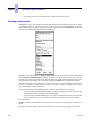

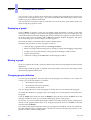
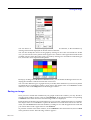
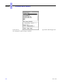

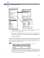
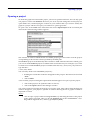
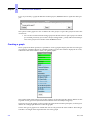

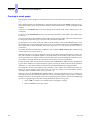
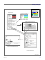

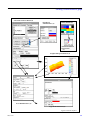


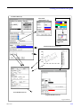

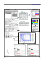


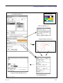


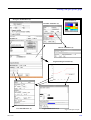
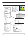


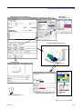

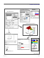
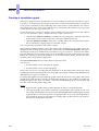

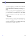


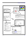

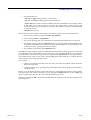

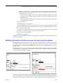
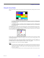
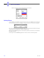


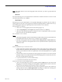
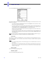
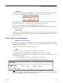

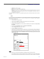
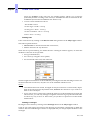
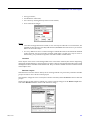

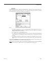

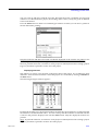
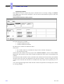
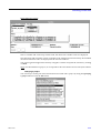
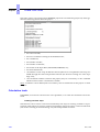
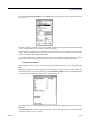
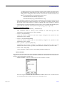
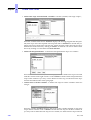
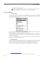


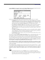
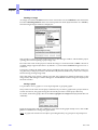


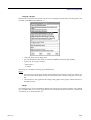
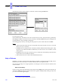


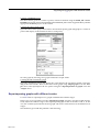
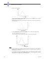
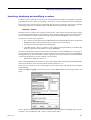
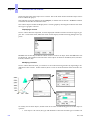
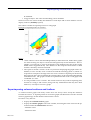

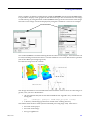
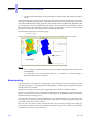

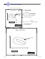
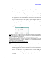
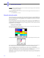
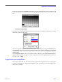

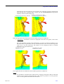

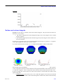

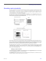
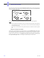

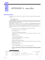

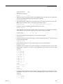
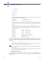


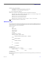


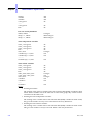
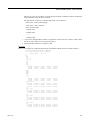
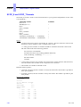
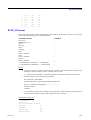
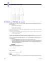


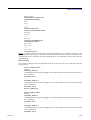
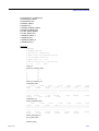
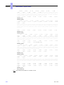


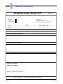


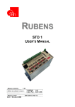





![[U4.33.01] Opérateur IMPR_FONCTION](http://vs1.manualzilla.com/store/data/006364725_1-cf170165efd19facb3106a56189ffb29-150x150.png)