1
Imaging Software
Olympus
User Manual
Family
We at Soft Imaging System GmbH have tried to make the information contained in this manual as accurate
and reliable as possible. Nevertheless, Soft Imaging System GmbH disclaims any warranty of any kind,
whether expressed or implied, as to any matter whatsoever relating to this manual, including without
limitation the merchantability or fitness for any particular purpose. Soft Imaging System GmbH will from time
to time revise the software described in this manual and reserves the right to make such changes without
obligation to notify the purchaser. In no event shall Soft Imaging System GmbH be liable for any indirect,
special, incidental, or consequential damages arising out of purchase or use of this manual or the
information contained herein.
No part of this document may be reproduced or transmitted in any form or by any means,
electronic or mechanical, for any purpose, without the prior written permission of
Soft Imaging System GmbH.
Windows, Word, Excel and Access are trademarks of Microsoft Corporation which can be registered in
various countries.Adobe and Acrobat are trademarks of Adobe Sytems Incorporated which can be
registered in various countries.
© Soft Imaging System GmbH
All rights reserved
Soft Imaging System GmbH, Johann-Krane-Weg 39, D-48149 Münster, Tel. (+49)251/79800-0, Fax.: (+49)251/79800-99
E_CELL_0206
Contents
Before you begin .......................................................................................1
First Steps .................................................................................................2
The (GUI) User Interface ..........................................................................................2
Saving GUI configuration .......................................................................................10
Printing images .......................................................................................................11
E-mailing images ....................................................................................................13
Button Bars .............................................................................................17
The Standard button bar ........................................................................................17
The Acquisition button bar ......................................................................................17
The Stack Navigator button bar ..............................................................................18
The Image Analysis button bar ...............................................................................24
The Image Display button bar ................................................................................24
The Image Stack button bar ...................................................................................24
Report Generator ....................................................................................25
Creating reports ......................................................................................................25
Saving / Exporting report ........................................................................................29
Report objects ........................................................................................................30
Report templates ....................................................................................................54
Planning report templates ......................................................................................61
Archiving Images ....................................................................................63
Define a database ..................................................................................................63
Insert data ..............................................................................................................72
Work in the database window ................................................................................82
Archive data ...........................................................................................................95
Protect with a password .........................................................................................99
Acquiring images ..................................................................................102
Acquire .................................................................................................................102
Snapshot ..............................................................................................................102
Camera Control ....................................................................................................102
Camera Configuration... .......................................................................................102
Set Input... ............................................................................................................111
intelligent Exposure ..............................................................................................113
Multiple Fluorescences .........................................................................................114
Acquire Z-stack... .................................................................................................125
Extended Focal Imaging .......................................................................................128
Define Image Sequence... ....................................................................................134
Multiple Image Alignment .....................................................................................139
The Image menu ....................................................................................152
Image Display .......................................................................................................152
Calibrate Image... .................................................................................................165
Set Magnification... ...............................................................................................167
Scale Bar ..............................................................................................................167
Overlay Bar ..........................................................................................................172
Delete Overlay ......................................................................................................181
Show Markers ......................................................................................................181
Contents
Define ROIs... .......................................................................................................181
Set Frame .............................................................................................................185
Enable Frame .......................................................................................................185
Convert .................................................................................................................185
Separate ...............................................................................................................187
Extract... ...............................................................................................................188
Combining fluorescences... ..................................................................................188
Edit Image... .........................................................................................................190
Copy Image ..........................................................................................................192
Delete Image ........................................................................................................192
Protect Image .......................................................................................................193
Define Image History... .........................................................................................194
Image Information... .............................................................................................194
The Process menu ................................................................................198
Intensity ................................................................................................................198
Adjust Colors ........................................................................................................208
Set Thresholds .....................................................................................................211
Binarize ................................................................................................................219
Define Shading Correction... ................................................................................220
Shading Correction ...............................................................................................222
Background Subtraction... ....................................................................................223
General Information on Filter Operations .............................................................224
Define Filter ..........................................................................................................228
Filter .....................................................................................................................242
Image Calculator... ...............................................................................................247
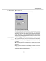
Arithmetic Operations... ........................................................................................250
Define Processing... .............................................................................................251
Execute Processing ..............................................................................................254
Image Geometry ...................................................................................................255
RGB-Studio ..........................................................................................................258
Spectral Unmixing ................................................................................275
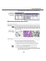
Interactive Image Measurement ..........................................................280
Save, Load and Edit Measurement Results .........................................................282
Create measurement sheets ................................................................................284
Using Statistics Functions ....................................................................................286
Measuring Arbitrary Structures .............................................................................288
The Measure menu ...............................................................................292
Pixel Value ...........................................................................................................292
Histogram .............................................................................................................292
Pixel Map... ...........................................................................................................292
Grid... ....................................................................................................................294
Intensity Profile .....................................................................................................295
ROI .......................................................................................................................297
Kinetic... ................................................................................................................298
Phase Color Coding .............................................................................................300
Phase Analysis .....................................................................................................301
Define Classification... ..........................................................................................302
Define Statistics... .................................................................................................304
Contents
Statistics ...............................................................................................................305
Graph .....................................................................................................307
Markers and Labels ..............................................................................................313
Set Split Gain... ....................................................................................................316
Modify Split Gain... ...............................................................................................316
Protect Graph .......................................................................................................317
Delete Graph ........................................................................................................317
Calibration ............................................................................................................317
Overlay Selection... ..............................................................................................319
Measure ...............................................................................................................319
Calculation ............................................................................................................321
Filter .....................................................................................................................323
Arithmetic .............................................................................................................324
Graph Information... .............................................................................................325
Define Graph History... .........................................................................................326
Convert to .............................................................................................................327
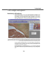
The Stage Navigator .............................................................................328
Summary of Features ...........................................................................................328
Preconditions for using the Stage Navigator ........................................................329
Start Stage Navigator ...........................................................................................330
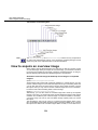
How to acquire an overview image ......................................................................331
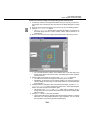
Save overview image ...........................................................................................335
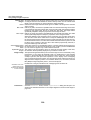
Loading an overview image in the Stage Navigator .............................................336
Deleting images ....................................................................................................336
The Modi of the Stage Navigator ..........................................................................336
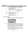
Change Stage Navigator Properties .....................................................................338
Acquire parts of the overview image with a higher magnification .........................340
Zooming in on an image .......................................................................................341
Adding Stage Navigator positions ........................................................................342
Moving to Stage Navigator positions and editing them .......................................342
Trouble Shooting ..................................................................................................343
Before you begin
Before you begin
Before you begin
The software package you have chosen was created by Soft Imaging System. You
have thus entered into the worldwide user community of our image analysis systems.
Welcome. The broad range of functions for digital image acquisition, image
processing, analysis, database archiving and results documentation, are all at your
disposal.
We think you’ll find working with cell a tremendously satisfying experience!
Warning
Your image analysis software is available in a great variety of expansion versions
and configurations. For this reason it is quite possible that in this manual functions
will be described that are not contained in the software package that you use, or that
inversely, certain functions that are available to you are not described here.
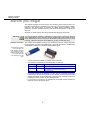
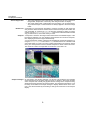
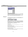
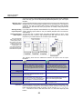
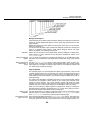
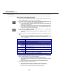
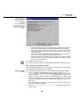
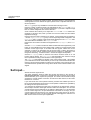
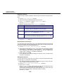
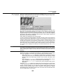
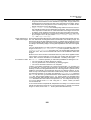
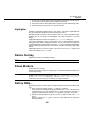
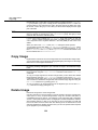
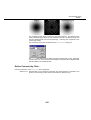
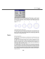
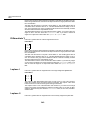
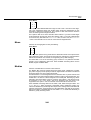
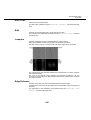
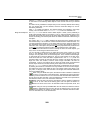
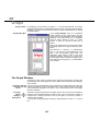
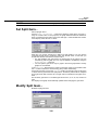
Software Protection The software is protected by a dongle. It is standard that an LPT dongle, that has to
be plugged into your computer's parallel port, comes with the software. USB dongles
are required for laptops or computers without parallel ports.
The software is protected by a dongle. The
USB dongle is delivered
as a standard. It is illustrated on the left and the
LPT dongle used with
the parallel port on the
right.
• cell can neither be installed nor started without a dongle.
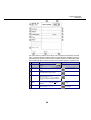
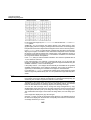
• The dongles are differently colored depending on their type:
USB-Dongle LPT-Dongle
Scope of license
blue
white
unlimited single license
black
blue
limited time dongle which only grants the user access to
the software for a limited period of time.
red
red
network dongle
• A network dongle can be plugged in to any one of a network's computers.
•
Please keep in mind that before cell can be installed, the driver software for the
network dongle has to be installed first. The Setup menu includes an option for
installing the driver software for the network dongle.
If your printer is connected to the parallel port, the dongle must be inserted between the PC and the printer cable.
1
First Steps
First Steps
First Steps
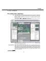
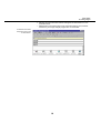
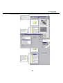
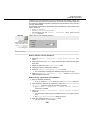
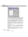
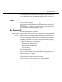
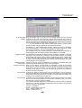
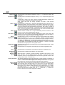
The (GUI) User Interface
GUI The graphical user interface influences the appearance of a program. It determines
which menus there are, how the individual functions can be called up, how and where
files, e.g., images, are displayed, and much more. This chapter describes the basic
elements of a GUI.
Please note: The Graphical User Interface (GUI) in your image analysis program is
fully adaptable to meet your own specific requirements.
Menu bar Many commands are accessible via the relevant menus. You can configure the menu
bar to suit your requirements. Use the Special > Define Menu Bar... command to add,
alter or remove menus as you wish.
Image buffer box Each image is allotted its own image buffer within your image analysis program.
When you start up your image analysis program all available image buffers will be
empty. While you use the program they will become filled - when you load or acquire
images, and when you perform various image operations that alter an image in such
a way that a new image results. During any given work session, this means that many
images are accessible simultaneously. Only one image buffer however, can be
active at any given time.
Related topics
Saving GUI configuration 10
2
First Steps
The (GUI) User Interface
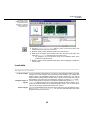
Active image buffer
• The image displayed in the image window, will always be the one in the active
image buffer, irrespective of how many other images are also on display.
• The active image buffer contains either the live image or an acquired image.
Any interactive input or measurements are always applied to the active image
buffer.
Button bars Commands you use frequently are linked to a button providing you with quick and
easy access to these functions. Please note, that there are many functions which are
only accessible via a button bar, e.g., the functions required for editing an image
overlay. Use the Special > Edit Button Bars... command to make button bars look the
way you want them to, and include what you need..
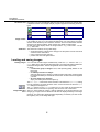
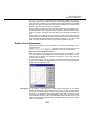
Viewport A viewport is a window in the image window where each of the loaded images, or the
live image is displayed. You can divide the image window into numerous viewports,
thus displaying numerous images simultaneously.
You can set both the number of viewports to be displayed and their arrangement, by
using the Arrange Viewports button in the Image window's button bar. This button will
open a field made up of 4x4 icons, each of which represents its own viewport. Simply
move your mouse pointer over the schematic viewports to select columns and rows.
The maximum number of images that can be shown at one time is 16.
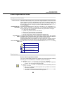
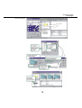
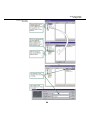
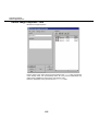
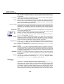
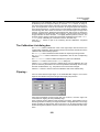
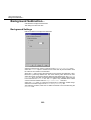
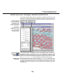
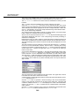
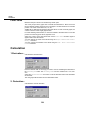
Viewport manager On the image in the viewport manager you will see a red rectangle. The rectangle
shows the segment of the image that is currently on display in the image window's
active viewport. That naturally only applies when the image in the viewport is being
displayed at a larger size than the viewport itself is. The rectangle is interactive: It can
be freely moved within the viewport manager to display different areas in the viewport. It can also be resized by mouse drag to change the zoom factor in the viewport
display.
3
First Steps
The (GUI) User Interface
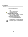
Within the thumbnail in
the viewport manager
you can define which
image segment is to be
displayed within the
image window. To
define the segment,
adjust the size of the
frame and move it to
where you want it within
the Navigator.
You can hide the viewport manager to create more room for other windows, for
example: To do so, use the [Alt+1] key stroke.
Note
Move the mouse pointer on the viewport manager and rightclick to open a context
menu.
Image manager The image manager contains numerous tabs. Click the different tabs to alter the
appearance of the image manager. The first two tabs List and Gallery are reserved
for the administration of images.
Note
Move the mouse pointer on the image manager and rightclick to open a context
menu. You can change the appearance of the image manager. To do so, use the
Image Manager Properties... command.
The operands box is for:
• determining source and destination image buffers used in image processing operations which alter the original image, e.g., inversion.
• linking images for certain image processing operations, e.g., addition of two images.
Use the image buffer box:
• for an overview of the images loaded,
• for rapid access to image information, such as its size and image type,
• to activate image buffers.
You can hide the image manager to create more room for other windows, for
example: To do so, use the [Alt+2] key stroke.
4
First Steps
The (GUI) User Interface
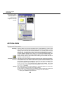
Document Area Documents can only be displayed within this area. Each document is opened within
a separate window. Your image analysis program supports the following document
types.
Image
Database
Text
Diagram
Sheet
Graph
Report
3D-Workspace
Image window The image window is a special window for viewing either loaded and/or live images.
It is possible to view up to 25 images simultaneously. For this purpose the image
window will be divided up into numerous windows. Such a window will be named a
viewport in the text that follows. Each viewport can display a single image.
To alter the image display within the image window - e.g., zoom factor - use the
Image button bar.
Status bar The status bar contains, among other things:
• a brief descriptions of all functions. Simply move the pointer over the command
or button for this information.
• name of the active input channel,
• position and size of the global frame.
Loading and saving images
Loading images You can load several images simultaneously. Click the Open button in the Open
Image dialog box to load all selected image files. The image files will be loaded into
successive image buffers. The first image buffer is the active image buffer.
To select...
• a continuous group of images: Then, while pressing [Shift], leftclick on the
last image.
• an arbitrary selection of images
select the first image by clicking on it with the left mouse button. Keep the [Ctrl]
key depressed while you use the left mouse button to select all of the image files
you want.
• all of the images in a directory:
simply use the keyboard shortcut [Ctrl+ A].
The File > Open... command is context-sensitive. This means the Open Image dialog
box only appears if an image window is active. If a text document is active the Open
Text dialog box will appear, etc.
The Open button is in the Standard button bar. To have a look at the dropdown list
of all the various commands for opening, click the arrow next to this button.
Image-buffer-box After you have loaded an image, it will be displayed in the image manager. The
icons image type, image name and resolution will also be displayed directly in the image
manager. The information displayed differs depending on whether you have set the
list or gallery view, in the image manager.
5
First Steps
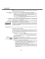
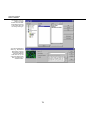
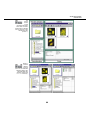
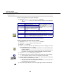
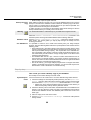
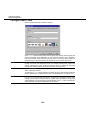
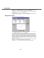
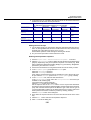
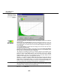
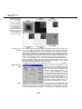
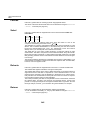
Available image types
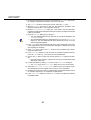
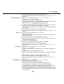
The image shown here
is a multi-channel image
that is made up of three
single frames. Each
frame is 1376 Pixels
wide and 1032 Pixels
high. Each single frame
has a 16-bit depth of
information.
Saving
images
Note
You save individual images with the File > Save As... command. You should save
your images as TIF files. Only when using TIF format are the additional image
attributes (overlay, image calibration, channel data, microscope data, image
comment) saved together with the image.
Please note, that even multidimensional images do not have their own file format
but are saved as TIF files. Do not use other file formats as the TIF format to save
multidimensional images in order to maintain all the information.
Available image types
Your image analysis program supports a large number of image types. These can be
divided into two groups of image types: the multidimensional images and the standard images. In the image manager different image types are represented by
different colored icons.
Note
Many functions of your image analysis program are only available for special image
types.
Multi dimensional Your program has also been designed especially for working with multidimensional
image images. Multi-dimensional images are made up of a number of images that have
been acquired one after the other. During the acquisition, the Z position and/or the
wavelength, and/or the time, will have varied from image to image. In other words,
multi-dimensional images are monochrome or multicolored images that are characterized by having an additional dimension. This additional dimension can be one of
space, (the Z-position has been varied) and/or of time (the position has been varied
on a time scale).
For displaying multidimensional images use the Image Navigator button bar.
A monochrome image consists of only one color channel.
A single color Z-stack image consists of monochromatic images which were
sequentially acquired at various focal planes.
A single color time-lapse image consists of single monochromatic images
which were sequentially acquired at different times.
A single color Z-stack in time-lapse image consists of single color images
which were sequentially acquired at different focal planes and at different
times.
A multi-channel image is made up of several monochrome images. Each
image stands for one color channel.
A multi-channel Z-stack image consists of multiple color images which were
sequentially acquired at different focal planes.
6
First Steps
The (GUI) User Interface
A multi-channel time-lapse image consists of multiple color images which
were sequentially acquired at different times.
A multi-channel Z-stack in time-lapse image consists of multiple color
images which were sequentially acquired at various focal planes and at
different times.
Standard images Your program can, naturally also cope with established standard formats. Standard
images can be depicted as three-dimensional data sets, the three dimensions being
two spatial dimensions (x, y) plus the wavelength (color value).
A gray-value image can be made up of 256 (8-bit), or 65536 (16-bit), gray
values.
A binary image is comprised of 2 gray values - black and white.
A false-color image is a gray-value image whose gray-values are shown in
color.
A true-color image, or RGB image, is made up of 16777216 colors (24-bit).
A Fourier image is a 32-bit image made up of real and imaginary numbers of
16 bits respectively.
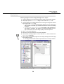
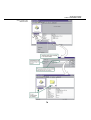
Loading images stored on the hard drive
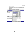
1) In the Image Manager, click on the image buffer you wish to load the image into,
with the left mouse button. Activate - for example - image buffer #5.
" The image buffer selected will be color highlighted and assigned to the
active viewport.
2) Select the File > Open... command to load an image.
" The Open Image dialog box will appear.
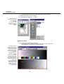
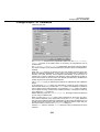
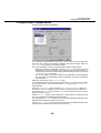
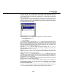
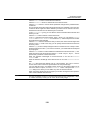
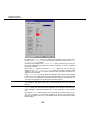
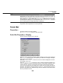
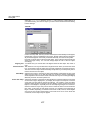
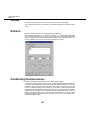
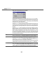
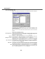
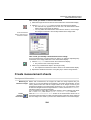
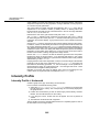
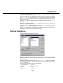
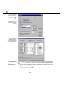
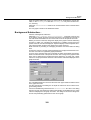
Dialog boxes for loading
files are based on standard MS Windows
dialog boxes. The dialog
box for loading images
also has a preview function.
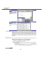
3) Select Tagged Image Format (*.tif), the standard image format, in the Files of
type list.
Warning
Please note that, since multidimensional images do not have their own file format,
they have to be saved as TIF files. You should only use the TIF format to save multidimensional images since only in this format will all of the information be saved with
it.
7
First Steps
Available image types
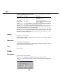
The Files of type list is
present in all dialog
boxes used for loading
documents. It provides
file formats for all document types.
4) Click the Up One Level button to move up a level in your computer's directory
structure.
" In the field below the button bar you will find a list of all sub-folders and
documents of the file types selected.
5) Doubleclick on one of the folders listed to get a listing of its contents - i.e., all
subdirectories and files the folder contains.
• Your program's root directory contains the "Images" subdirectory. In it you
will find a selection of TIF images.
6) Click the Preview button to view thumbnails of image files. Select the image files
one at a time.
7) Select the images you wish to load.
8) Click the Open button to load the images selected.
" The Open Image dialog box will be closed.
" The images will be loaded into successive image buffers. The first image
will be loaded into the active image buffer, e.g., #5. The next images you
load will then be inserted into image buffers 6-9 (if you have loaded a total
of 5 images simultaneously).
Activate image window
Sometimes the image window will be hidden behind another window. This is the case
if a document window has been maximized or if numerous other documents have
been opened. The following step by step instructions show you only one of the ways
of bringing the image window back to the foreground.
1) Select the Window > Document-Manager... command or use the [Alt+3] key
stroke.
" You will find all of the open document windows listed in the document
manager. The document type and the title of the document window are
given for each document.
2) Select the image window.
" There is always just one image window!
3) Click the Activate button located in the document manager.
" The image window will then be in the foreground.
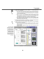
Loading images into specific image buffers
1) Click the Gallery tab in the image manager.
2) Activate the image window by simply leftclicking within the window.
• If the Images window's header is colored, this means it is active.
3) Select the Standard (button bar) > Open... command.
4) Leftclick on the image file you wish to load.
5) Drag the file directly onto any one of the image buffers while keeping your left
mouse button pressed, (drag&drop).
8
First Steps
The (GUI) User Interface
" The image buffer will show a preview of the image you have loaded.
6) Repeat the last step as often as needed.
7) To quit loading, just click the Close button.
Use the mouse to
drag&drop images into
the image buffer
desired.
MS Explorer, a file
manager, can also be
used for drag&drop
loading.
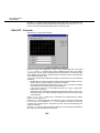
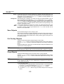
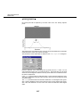
Optimizing display
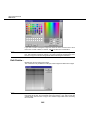
1) Press [Ctrl+Alt+T] to generate a test image.
• The image window contains a button bar with which you can quickly alter
the appearance of the images in the image window.
Press [Ctrl+Alt+T] to
generate a test image. It
will have a color image
overlay which displays
current monitor resolution and other information. Press
[Ctrl+Alt+Shift+T] to
generate a color test
image.
The test image will automatically be the same
size as the active viewport. The test image will
always be displayed at
100% zoom.
The header shows the
number of the image’s
image buffer, (2), the
image name, (Test),
and the current zoom
factor (100%).
9
First Steps
Saving GUI configuration
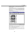
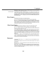
2) Click the Arrange Viewports button to redefine the number and arrangement of
viewports. Select a 1x2 arrangement.
" The image window will be divided up into two viewports. The test image is
in the left viewport. Image buffers will be reassigned. Zoom factors will be
set to Auto. Although somewhat reduced in size, the entire test image will
be shown.
3) Click the Single View button to display just one image in the image window - the
active viewport image.
" The viewport arrangement and what image buffers are shown in which
viewports remain unchanged.
4) Select one of the predefined options in the Zoom Factor dropdown list - or enter
the zoom factor you want, directly in the field; e.g., 30%.
" The test image will be reduced to 30% zoom. The viewport will no longer
be totally taken up by the image. Where the patterned background starts
(in the viewport) is where the image stops.
5) Click the Zoom In button to double the current zoom factor.
" The test image will now be displayed at a zoom factor of 60%.
6) Click the Adjust Zoom button to have the zoom factor adjusted to fit current
viewport size.
• The length/width ratio of the image will not change. Unlike the automatic
zoom factor, this zoom factor is not linked to the size of a window - i.e.,
even when you adjust the size of a window, the zoom factor stays the
same.
7) Alter the size of the image window.
8) Click the Adjust Window button to have window size adjusted to fit current
image size.
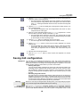
Saving GUI configuration
Workspace You can save your graphical user interface in a file. The current user interface is
called a workspace. A workspace includes the layout of all document windows and
button bars as well as how viewport and image manager are positioned. It can also
include specific images and documents you wish to have loaded.
• Defining GUI layout
You may want to define workspaces for each of the various kinds of tasks, thus
optimizing how the graphical user interface is laid out for each of these. Separate workspaces could be for image acquisition, report generation and image
analysis. Having separate workspaces gets you the onscreen layout you need
and fast.
• Reloading images/documents
The path names of currently loaded images and documents can be saved in a
workspace. Saving the current GUI in a workspace at the end of your workday
makes it totally easy for you to continue where you left off the next morning. Any
and all images, sheets, diagrams, database(s), report(s) that were loaded when
you saved the workspace will be right where you left them.
Warning
Be sure to save all your images before shutting down your image analysis program.
Any unsaved images will be deleted without prior warning.
Configuration The Special > Configuration command enables you to individually determine
versus Workspace elements on your user interface, as well. Please note that the configuration and workspace contain different elements of the user interface. Configuration refers to what
10
First Steps
Printing images
commands have been defined for menus, button bars and keyboard, e.g., userdefined button bars. A configuration saves what functions are available on your GUI.
A workspace, however, actually saves what the GUI looks like, including specific
documents. The information saved in workspaces and configurations is totally
different.
Please not that there is a default workspace for working with reports. Use the [Ctrl+2]
key stroke to load this workspace.
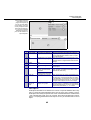
Printing images
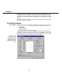
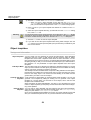
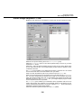
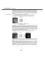
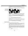
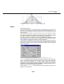
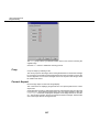
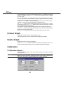
Print Templates You can determine the print template for different document types. To do so, use the
File > Define Page Layout... command. The template contains the page layout of:
• single images
• multiple images
• database images, and
• other documents, e.g., sheets and diagrams.
A page layout consists of header/footer definition and the position and magnification
of images. The report generator gives you many more possibilities as well as very
complex page layouts. The report generator, which is integrated into your image
analysis program enables you to design a page independently.
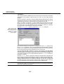
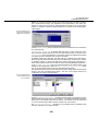
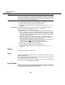
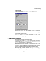
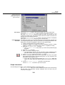
You define your own
standard page layout
for: printing out single/
multiple images, or database images, and for
printing out text, sheets,
diagrams and graphs as
well.
11
First Steps
Printing images
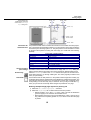
The illustration describes terms which are
used in the Define Page
Layout dialog box.
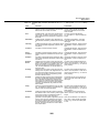
Field codes for Use predefined field codes in headers and footers to have certain document properheaders/footers ties or information automatically included in your documents. Field codes are always
introduced by the following symbol: "$". They are placed in curved brackets. To have
an image’s name printed out along with the image you would enter the following:
${Name}.
${Name}
${Comment}
${Buf}
${Page}
${PrintMag}
${Date}
${Time}
${Now]
Field codes in headers/footers
image or document name
image comment
image buffer number
page number
on-paper image magnification
image creation date
time of image creation
time at printout
Context-sensitive The File > Print... command is context sensitive and thus dependent on what kind of
print settings document is active. If the active document is an image, the Print Image dialog box
will be opened. Different document types open respectively different dialog boxes.
Print Directly
Click the Print Directly button in the Standard button bar to print out the active document without having to go through a dialog box. The active page layout will be used
when you print directly.
Draft mode
Use the draft mode for trial printouts. In the position where images are located, gray
rectangles will be printed. Headers and footers will also be printed as rectangles. The
actual images will not be printed out, as image prints can be time consuming. Draftmode printing is a fast and easy way to check out what your layout looks like, e.g.,
when you just want to see exactly where images are positioned on a page.
Defining multiple-image page layouts for printing out
1) Select the File > Define Page Layout... command.
2) Select the Single Image tab to define header and footer position.
• Define borders in cm in the Border group. Have a look at the illustration
(previous page) to see what the various fields are for.
• Both headers and footers may have multiple lines of text. If the text is too
long it will not be completely printed out, i.e., it will be cut off when the page
is printed.
12
First Steps
E-mailing images
• Select the Fixed image ratio check box to maintain the image’s original
length/width ratio when printed out.
3) Select the first Header/Footer tab (the first one on the left, going left to right) to
define headers and footers for the whole page.
• Enter the text desired in the Header and Footer fields: e.g., "page ${Page},
date ${Today}", to have the page number and current date printed on the
page.
4) Select the second Header/Footer tab to define a different caption for each
image.
• Enter, e.g., "${Name}" in the Footer field to have the image’s name printed
beneath the image automatically.
• Select the Print scale bar check box to have a scale bar printed beneath
each image.
• Select the Print page header/footer check box to have the page headers
and footers defined in step 3 also printed when you print out.
5) Select the Multiple Images tab to define the images’ position on the page.
• Define how images are to be positioned when printed out in the Image tiles
group.
Enter the number of images to be printed out ‘across’ (i.e., horizontally) in
the Horizontal field, and the number of images ‘down’ (i.e., vertically) in the
Vertical field.
• Define the distance between images and the distance to the headers and
footers in the Border group. Page borders will be defined according to the
Single Image tab.
6) Click the Print... button to open the Print Image dialog box. Once your have
defined the page layout one time, you can simply select the File > Print...
command for any future printouts.
7) Select Multiple Images in the Page layout list in the Print Image dialog box.
• This list also includes Single Image to have images printed out one per
page.
8) Select the All images option in the Print images group to print out all images
currently loaded.
• If your have selected the Range of images option, you will need to enter
the corresponding image buffer numbers into the field below this option. If
you enter, e.g., '4-7,3' - the images in image buffers 4, 5, 6, 7, 3 will be
printed out.
9) To start printing, click on OK.
" The number of pages printed will automatically refer to the number of
images selected.
E-mailing images
Background Information
The following is The File > Send email... command is only available if:
required
• documents are loaded (e.g., an image and a report), and
• you have installed a MAPI-supported e-mail program and MAPI.DLL file.
13
First Steps
E-mailing images
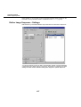
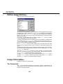
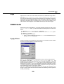
Sending work- Select the Add a workspace for the selected documents check box in the Send email
spaces via e-mail dialog box to include a Workspace.wos file along with the other documents you’re
e-mailing.
The recipient can thus open the workspace along with all images and documents and
display these in their original onscreen arrangement. To do this, the recipient will
have to save all attachments in a separate directory. To open a workspace along with
all other documents, select the File > Workspace > Open... command.
The size of your e- To receive a warning message when the size of your e-mail attachments exceeds a
mails certain limit (which you may set yourself), go to the following tab: File > Send email...
> Preferences > General. The following are possibilities to reduce the size of your
e-mail:
• Leave out some documents.
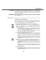
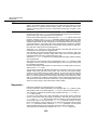
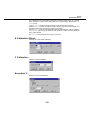
• Compress images. Go to the Image and Report tabs in the Send email Preferences dialog box to do this.
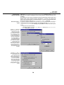
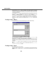
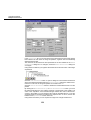
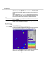
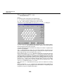
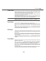
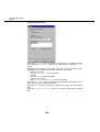
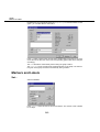
Use the Image tab to set
the file format for all images that you e-mail.
The Save Image Options dialog box enables
you to determine for the
TIF format whether or
not and how the images
are to be compressed.
You define whether or
not 16-bit images are
automatically converted to 8 bits, and whether
image overlays are
burnt into the image before being sent. Please
note that the options for
saving images are not
the same for all image
formats.
Use the Report tab , to
determine the file format
for the reports to be
sent. The RTF format
has two advantages for
the sending of reports:
you can considerably
reduce the report's file
size, and the recipient
can open the RTF file
report in other application programs, e.g., MSWord.
14
First Steps
E-mailing images
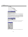
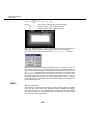
How to e-mail...
1) Open all the documents and images you wish to send in an e-mail.
• If you’re planning on sending database images and documents, open the
database(s) and select the records desired.
2) Use the File > Send email... command.
" The Send email dialog box lists all images and documents currently
loaded/open in your image analysis program.
• All the files in this document list are selected by default.
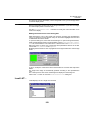
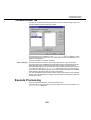
The above figure shows
a list of all types of documents that can be emailed via your image
analysis program as
well as their respective
standard formats.
3) To clear all selections, simply click the Unselect All button. Select the documents you’re interested in by clicking on the corresponding check box in the
document list.
• A warning message will appear if your attachment exceeds a maximum
size!
4) Select the Add attached database documents check box to send a record and
any appended documents (images, sheets, graphs etc.).
• An entire image database cannot be sent via e-mail.
5) Click the Preferences... button to set file formats for all images, sheets,
diagrams and graphs.
" The Send email Preferences dialog box will be opened.
6) Select the Image tab in the Send email Preferences dialog box to define the
image file format. File formats are always defined for all the respective documents of one single type - not for one single document.
• The TIF format is default. Select the Burn overlay into image and Convert
16-bit images to 8-bit check boxes for this file format if the recipient will
open the images with another application program. This will be automatically done for all other image formats.
• If possible, compress the images to keep the size of the e-mail to a minimum. Use the JPEG image format if the recipient wants to open the images with another application program since most application programs cannot load compressed TIF images.
7) To determine the file format for sending reports, select the Report tab located in
the Send email Preferences dialog box. Select the Send report in Rich Text
Format(*.rtf)option if the recipient wants to open the report in another application program, such as MS-Word. For RTF format, you can reduce the resolution
of the images in the report.
8) Close the Send email Preferences dialog box by clicking on OK.
9) Please Note: Select the Custom option in the Send email dialog box to activate
the format settings your have just made.
10) Click the Send... button.
15
First Steps
E-mailing images
" All image and document files selected will appear as attachments in a new
e-mail document.
• Please keep in mind that as long as the e-mail document is open, all other
functions in your image analysis program are not accessible.
All selected documents
will appear in the e-mail
as attachments.
16
Button Bars
Button Bars
Button Bars
Some functions are only available via the standard button bars. This chapter
describes the most important button bars.
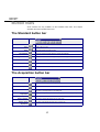
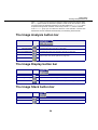
The Standard button bar
New
Creates a new text document.
Open
Loads a file from disk.
Save
Saves the active document to disk.
Print Directly
Image Information
Protect Image
Prints the active document with the current print settings.
Displays an overview of all image data (see also on page 194).
Toggles the read only mode for the active image buffer on/off.
Copy
Copies the active image or selection to the clipboard.
Paste
Pastes the contents of the clipboard.
The Acquisition button bar
Acquire
Starts continuous acquisition using active input device.
Snapshot
Stops continuous acquisition or acquires single image.
Camera Control
Adjusts the camera parameters. For more information on the camera parameters click on the help button in the dialog box.
Define Fluorescence
Acquisition
Defines the acquisition of fluorescence images (see also on page 120).
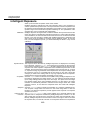
Intelligent Exposure
Starts up the automatic mode of the camera (see also on page 113).
Acquire Z-stack
Acquire Image
Sequences
Acquires an image stack (see also on page 125).
Acquires image sequences (see also on page 134).
17
Button Bars
The Stack Navigator button bar
Microscope Control
Acquire Fast Image Sequence
Opens the microscope control panel. For more information on the microscope
control click on the help button in the dialog box.
Acquires a fast image sequence as image stack.
The Stack Navigator button bar
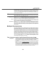
Multi-dimensional images consist of image stacks of different color channels, time
sequences or Z-stacks. With the commands in the Stack Navigator button bar you
can easily select single images out of an acquired image sequence to be displayed
in the viewport.
Select Color Channel
Only displays the selected color channel (see also on page 19).
Navigate Z
Chooses a projection in z-dimension for the direction of an image stack.
Navigate Time
Chooses a projection in t-dimension for the direction of an image stack.
Click one of the buttons Select Color Channel, Navigate Z or Navigate Time to
select the dimension you are interested in.
A multi-dimensional image, for example, consists of several color channels.
Click the Select Color Channel button first and the Next button afterwards to
step through the individual color channels.
First
Previous
Got to
Jumps to the first image.
Jumps one image back.
Jumps to a certain position.
Next
Jumps one image forward.
Last
Jumps to the last image.
Animate
Opens the Animate Image Stack dialog box (see also on page 22).
18
Button Bars
The Stack Navigator button bar
Select Color Channel
Use the Select Color Channel menu to set the display mode. The menu offers the
following commands:
All Color Channels
A multi-channel image is made up of several monochrome images.Each image
stands for one color channel.
For example: A sample is labeled with three different fluorochromes. The resulting
multi-channel image acquired with three different excitation filters is displayed as an
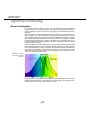
overlay of the three different color bands.
To view the individual color bands, open the Select Channel menu. All color channels
of the active image are listed. Select the desired color from the list. The currently
displayed color channels are marked in the shortlist. The selected color bands will be
displayed exclusively in the viewport; the other channels will be hidden.
You may select only one or more than one channel To select more than one channel,
keep the [Shift] key depressed when you select the channels.
Gray Scale
Uses a gray LUT for the single color channel display.
This does only change the display, not the image itself. Thus, you can simply switch
to another display mode.
Note that the display mode is part of the image information. If you save the image, its
current display mode is saved as well.
LUT: [Name of the LUT]
Uses a color LUT for the single color channel display.
Use the Image > Adjust Color > Load LUT... command to select the LUT to be used
for display.
Fluorescence Color
Uses wavelength LUT for the single color channel display.
Use the Edit Fluorescence Color... command to modify the color information to be
used for the display.
To open this dialog box, load a multi-channel image. To open the image information,
simply doubleclick the image in the image buffer. On the Image Information > Dimensions tab, doubleclick the color field next to a fluorescence.
19
Button Bars
The Stack Navigator button bar
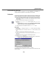
Load LUT
Use the Load LUT... command to set the LUT to be used for display in the FalseColor mode. The normal entry dialog box will open.In it you can select one of the
numerous predefined LUTs.
Click the Load button in this dialog box to load the selected LUT. The application
automatically switches to the False-Color display mode.
Overlay Transmission
Activates and deactivates the overlay mode.
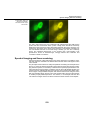
The selective fluorescence labeling of sub-cellular structures often creates an image
in which a particular cell is no longer visible. To enable you to see where the fluorescent structures in the cell are located you can overlay a fluorescence image with a
transmission image in the viewport, (when you do this, these images can be acquired
by contrast enhancing methods). You can only overlay them when both images have
an identical X/Y resolution. A multi-dimensional image can be overlaid either with a
single image (snapshot), or with a multi-dimensional image, whereby the number of
single images in the time-lapse image or Z-stack must be the same for both multidimensional images.
To create an overlay image of fluorescence and transmission images
1) Activate the fluorescence image; it can be monochromatic or multi-channel.
2) Open the menu of the Select Color Channel button and choose Select Transmission. A dialog box opens that lists the images that would fit for an overlay.
3) Choose the desired image and click OK.
" The viewport shows the resulting overlay image.
4) Deselect the Overlay Transmission command to remove the overlay.
Note
The overlay image is not a new data set; it only exists on-screen. To create an
overlay image as new data set use the Edit > Copy and the Edit > Paste command
(<Ctrl+c> and <Ctrl+v>) and store the new image. This image is a 3x8bit RGB
image, not an nx16bit image.
20
Button Bars
The Stack Navigator button bar
Select Transmission
Shows a dialog to select the transmission image.
Select the desired overlay image from the Available overlay images list. This list
contains all of the overlay images that are possible: All of the images in the image
manager that are of exactly the same size as the active image. The active image's
individual color channels also belong to the possible overlay images.
Click the OK button to have the selected image superimposed on the active image.
Navigate Z
In z (3D) experiments stacks of images are acquired at different focal planes. If the
active image buffer contains a Z-stack the Navigate z button is available in the Stack
Navigator button bar.
With the Previous and Next buttons in the stack navigator, you can navigate frame
by frame backward or forward. The First and Last buttons can be used to display the
first and the last image. The number within the field represents the number of the
currently displayed frame. You can directly go to a specific frame by typing the
respective number into the Go to field and pressing the [Enter] key.
The menu offers the following projection functions:
Single Z-Layer
One image of the-Z-stack is shown. Use the buttons of the Stack Navigator button
bar to select a Z-layer.
Maximum Intensity Projection
For each pixel in the XY-plane the intensities of the different Z-layers are compared.
The maximum intensity is used for display.
Mean Intensity Projection
For each pixel in the XY-plane the intensities of the different Z-layers are analyzed.
The mean value of all intensities is used for display.
21
Button Bars
The Stack Navigator button bar
Minimum Intensity Projection
For each pixel in the XY-plane the intensities of the different Z-layers are compared.
The minimum intensity is used for display.
Navigate Time
In time-lapse experiments the images are subsequently acquired, according to the
parameters defined in the time-lapse properties page, and stored as an image stack.
If the active image buffer contains an image stack containing a time sequence the
Navigate Time button is available in the Stack Navigator button bar.
With the Previous and Next buttons in the stack navigator, you can navigate frame
by frame backwards or forwards, respectively, through the time sequence. The First
and Last buttons can be used to display the first and the last image, respectively, of
the acquired time series. The number within the field represents the number of the
currently displayed frame. You can go directly to a specific frame by typing the
respective number in the Go to field and pressing the [Enter] key.
The menu offers the following projection functions:
Single time frame
One selected time frame is shown. Use the navigating buttons in the Stack Navigator,
button bar to select the image you want from the time-lapse image.
Maximum Intensity Projection
For each pixel in the XY-plane the intensities of the different time frames are
compared. The maximum intensity is used for display.
Mean Intensity Projection
For each pixel in the XY-plane the intensities of the different time frames are
analyzed. The mean value of all intensities is used for display.
Minimum Intensity Projection
For each pixel in the XY-plane the intensities of the different time frames are
compared. The minimum intensity is used for display.
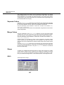
Animate Image Stack
Clicking the button opens the Animate Image Stack button bar:
22
Button Bars
The Stack Navigator button bar
Here you find the buttons to start (Play) the animation, to stop it and to play it in the
reverse mode.
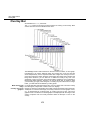
The slider displayed at the bottom of the Animate Image Stack button bar indicates
the position of the currently displayed frame within the sequence. Additionally, you
can define a sub-stack within the time-lapse image. Then, only the images belonging
to this sub-stack will be animated. To do so, move the slider to the desired starting
frame position and click the Mark In button. Then move the slider to a subsequent
frame, click on the Mark Out button to set the end frame for the slide show. The
selected frame scan will be highlighted in blue in the slider bar.
If you now press the Play button only the range of frames within the blue bar is
animated.
Click the Options button to define the parameters for the animated slide show.
In the Frame rate field you can adjust the number of frames displayed per second.
23
Button Bars
The Image Analysis button bar
In the Loops group you can choose how often the image stack is to be played. Select
the Play option to have the animation repeated n times. Enter the number of times
you want to have the animation repeated, in the field. Select the Auto Repeat option
to repeat the image stack animation continuously until the Stop button is clicked.
In the Direction group you can select the direction of the animation. Choose here
whether the stack is animated unidirectionally or meandering back and forth.
The Image Analysis button bar
Define ROIs
Intensity Profile
Background Subtraction
Calibration (Unmixing)
Defines the regions of interest (see also on page 181).
Calculates the kinetics (see also on page 298).
Calculates the background subtraction (see also on page 223).
Separates and resorts the contribution of different fluorochromes to the total
signal in each color channel (see also on page 275).
Unmixing
The Image Display button bar
Adjust Display
Auto Adjust Display
Load LUT
Adjusts the display of the image (see also on page 152).
Adjusts automatically the display of the image (see also on page 158).
Load display LUT for a single color channel (see also on page 160).
The Image Stack button bar
Combine
Extract
Combines different images in one (see also on page 188).
Extracts the selection (see also on page 187).
24
Report Generator
Report Generator
Report Generator
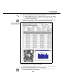
What exactly does Automatic report generation
report generator Use report generator to have multipage reports produced practically automatically,
do? including images of a database or of the image manager. Select a number of, (or lots
of) images from an image database and have them all added to a report using a
single command.
Full database-integrated access
Along with the images themselves that you get out of a database, you can have all
additional information on the images (contained in database fields of image databases) automatically included in a report. Sheets with important measurement
results can also be automatically filled in.
Working with images
A particular focus of report generator is being able to work with images in an optimal
way: norm enlargements are followed; detail zooms can be inserted; appropriate
image segments can be selected; and more.
Texts, Sheets, Diagrams, Graphs
Most types of documents that you generate within your image analysis program can
be inserted into a report. Via report generator, you can, e.g., print out images along
with related measurement sheets and diagrams on the same page.
Flexible Page Layouting
Report generator provides you with the most flexible page layouting imaginable: you
set up your own template pages exactly the way you want them to be. You generate
your template pages only once. These templates are the basis for your reports and
ensure that the appearance of your documents is uniform.
MS Word compatible
Via the RTF Export function, you can have reports exported to MS Word 1:1. This
enables you to communicate with fellow colleagues who may not have access to your
image analysis program.
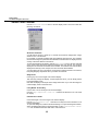
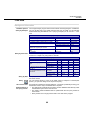
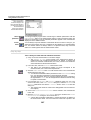
Creating reports
Background information
Reports and report Reports are used to document results in standardized form. They usually consist of
templates many pages which are similarly structured. In order to make report creation easier, a
report is based on a report template. The report template defines all page layouts and
object templates that can be used in this kind of report.
Report window You can never load and edit more than one report (or report template) at a time. The
report will be loaded into its own separate window. Only one report page can be
shown and edited in the report window at a time. The report window has its own
separate button bar and a status bar. There are ruled borders and a grid for use as
positioning aids.
Related topics
Exporting reports 29
Report templates 54
Ruler 32
25
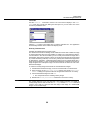
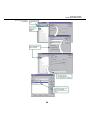
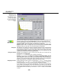
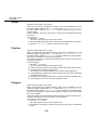
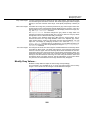
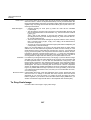
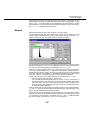
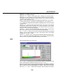
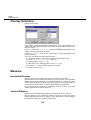
Report Generator
Creating reports
Reports are opened
within a separate window. The functionality of
the report generator is in
the button bars. The Report and Report Objects
button bars are the two
most important button
bars.
Report button bar The report button bar is a part of the report window. Please keep in mind that these
buttons’ functions are not available as menu functions. This is why this button bar
should remain visible. If you like, you can use the Special > Edit Button Bars...
command to show or hide the button bar or to add other frequently-used buttons.
Turning button bars
• Use the Special > Edit Button Bars... command.
‘on’ and ‘off’
• Rightclick in a report window. All button bars linked to report generator are listed
beneath the Button Bars command.
26
Report Generator
Creating reports
Paging through a You can only display one page in the report window. Use the first buttons of the
report Report button bar to leaf back and forth through a report. When paging, the current
report page will automatically be saved.
Go to
If you want to get to a particular page fast, enter the page number into this field and
confirm via [Enter].
Add Page
Click the Add Page button to add a page to the active report (at any place). After
clicking the button, select where the new page should be inserted. You can add a
new page either in front of the active report page or at the end of the report.
You have to indicate a page template for each page. This determines the pages’
appearance(s).
The newly-added page will become the active page, no matter what page was being
shown before the new page was inserted.
Delete Page
Click the Delete Page button, to delete the report's page which is currently displayed
in the report window. You have to confirm the deletion of a page. Any and all image
files and thumbnails in connection with the page will also be deleted. Images inserted
into a report as links will, of course, not be deleted.
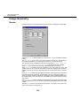
Report properties Define the page format for the current report in the Report Properties dialog box
(Border and Format groups). In addition, determine some of the properties of the
Graphical User Interface (GUI) (Grid and Ruler groups):
You can open this dialog box by rightclicking on any part of a report on which no
object has been placed and selecting the Properties... command from the context
menu.
File Format The file formats SRD and SRC are available for saving reports. Both formats are
exclusive file formats of your image analysis program and cannot be opened with
other application programs.
Select the SRC file type to place all files which belong to the report in a single
container file. If you insert a report in an image database, the report is automatically
inserted in SRC format.
When using the SRD file type, the report is not saved in a single file. Similarly to the
saving of a database, there are several files and directories involved. Any files that
are part of a report will be automatically placed in a subdirectory named after the
report. When making backup copies, the easiest thing to do is to copy the whole
report directory.
27
Report Generator
Creating reports
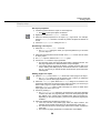
Step-by-step
Set report properties
1) Leftclick anywhere within the report on the background.
" Now none of the report objects is selected.
2) Rightclick and select the Properties... command.
3) Select the desired properties for the report, e.g., page format. For example,
clear the Snap to grid check box to be able to position all objects as desired via
mouse.
4) Close the Report Properties dialog box via OK.
Generating a new report
1) Select the File > Report > New... command.
" The New Report dialog box offers you report templates that you can base
your new report on.
2) Select the report template named "Normal" in the General tab in order to create
an empty report.
3) The Report option is default in the Create new group.
4) Confirm via OK to have the report generated.
" The first page of the new report will appear within a separate window. The
first page’s appearance is determined in the report template.
" Your image analysis program will display a number of button bars to be
used in making and editing reports. These button bars are context-sensitive, i.e., as soon as you activate another document the report button bars
will disappear.
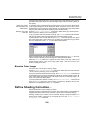
Adding pages to a report
5) Click the Add Page button in the Report button bar to add a page to the report.
" The Add Page dialog box will be opened. This is where you determine
where you want to add a page within the report.
6) Select the Insert page option within the Add Page dialog box to insert the new
page directly before the current report page. This is the option you choose if you
have to add a page to a report that is finished otherwise.
Select the Append page option to add a last page to a report no matter which
report page is the active one or not.
7) Confirm by clicking OK.
" The Add Page Template dialog box is opened if the used report template
contains more than one page template. You’ll find all template pages that
are defined in the current report template listed within the dialog box.
Depending on the report template, you’ll have very different page layouts
available.
8) Select the desired page template and confirm via OK.
" You’ll now see the newly-added page within the report window. The
selected report template page influences the appearance of the page.
" The status bar shows the current page and the total number of pages the
report has.
" The buttons for paging backwards or forwards are now available.
28
Report Generator
Saving / Exporting report
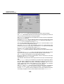
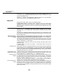
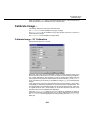
Saving a report
1) Press [F8] to open the Preferences dialog box and select the Report tab.
" You’ll find the standard path for saving reports and templates in the Directories group.
" Your image analysis program will propose a standard directory for saving
reports: the "Report" directory is a subdirectory of the root directory.
2) Enter the path name where you want to save your future reports into the Reports
field, e.g. "C:\Reports\ProjectXYZ".
• If the report directory does not yet exist, click the ... button next to the Reports field. Click the Create New Folder button in the Select Directory dialog box to set up the directory.
3) Confirm the new report path via OK.
4) Click the Save button in the Standard or Report button bars.
" If you are saving the report for the first time, the Save Report Document
dialog box will be opened.
" Your image analysis program will propose the report directory called
"C:\Reports\ProjectXYZ" in the Save in list.
5) Enter a content-relevant name for your report into the File name field.
6) Select the "report container (*.src)" from the Save as type list to save the report
in a single file.
7) Click Save to save the report.
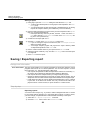
Saving / Exporting report
Background Information
Rich Text Format The RTF format enables you to transfer formatted text documents between various
programs that can be run on various platforms. You can save reports in an RTF
format and then, e.g., load and edit them in MS Word.
• RTF reports are optimized for MS Word (MS Word versions 97 and later), i.e.,
the report’s layout remains unchanged when loaded into MS Word.
• RTF reports cannot be reimported into your image analysis program.
• Images are always inserted into an RTF file as copies and not as links. This is
always the case no matter how the images were inserted into the original report.
• In MS-Word, RTF files can only be displayed and edited in the Layout, or Online
Layout view. In the Normal or Outline view, only continuous text will be displayed in Word. In terms of Word, a report contains no continuous text.
Step-by-step
Exporting reports
You want to send a report, e.g., by e-mail, to fellow colleagues that have no access
to your image analysis program (or to the image files involved). In order to do this,
you need a single, complete file that contains all data necessary to the report.
1) Select the File > Report > Export RTF... command.
2) Click the Browse... button next to the Destination file field.
29
Report Generator
Report objects
3) Select the directory for the RTF file in the Save RTF dialog box. Enter the name
of the RTF file into the File name field. Click the Save button to return to the
Export RTF dialog box.
" The complete path and file name of the RTF file is now located in the Destination file field. Note that the RTF file has not yet been saved.
4) Determine the resolution of the images in the RTF file and thus the file size of
the RTF file in the Reduce image data group. If you are planning on sending
someone the report by e-mail, then it makes sense to keep file size as small as
possible.
Select the Use JPEG compression check box.
5) Enter 60 into the quality [%] field. This quality value determines the degree to
which images are compressed (low percentages mean a correspondingly high
degree of compression).
" The JPEG compression reduces the file size of an image but also generates typical image artifacts. The more you compress an image, the greater
the loss in image quality. JPEG artifacts are generally not visible in a
printout at 60%.
6) Initiate exporting by clicking on OK.
" The resulting RTF file you can now, e.g., load in MS Word or send to
someone by e-mail. The layout of the report remains completely
unchanged in MS Word.
• The file size of RTF files can be very large. You can reduce the file size by
saving the report in MS-Word as a Word document in DOC format.
Printing the report
1) Select the File > Print... command to print out the finished report.
" The Print dialog box is context-sensitive. This simply means that the functions being offered by the dialog box depend on what document is active.
Before you print a report, you have to activate this dialog box.
2) Select the Full image option from the Images group within the Print dialog box.
3) Select the All option from the Print Range group to have the report printed out
in its entirety. Start printing by clicking on OK.
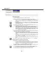
Report objects
Background Information
Report objects A report page usually includes various kinds of objects. These may involve image
and text objects as well as graphic objects. For each object there are individual characteristics which can be defined, which are different for each object type. A certain
object type, the record object, can consist of numerous other objects. You can define
individual object templates for record objects. In doing so, you not only create a
wealth of different record objects, but also guarantee a uniform appearance of the
record objects in different reports.
Placeholder Several objects serve as placeholders. Image objects and record objects are typical
placeholders. These objects are usually defined in a report template. If you then
create a report based on this template, the placeholders are filled with concrete
images or database information. Diagrams, sheets and single sheet cells can be
30
Report Generator
Report objects
Background Objects
autotext
Selecting objects
Selecting several
objects
Object Properties
defined as placeholders.
Use a placeholder’s properties, e.g., size and position to define the properties of
images or texts you wish to later insert into a report.
Background objects are defined on the template page and appear on each page of
the report which is based on this template page. A company logo, address, or frame
are common background objects.
AutoTexts are texts defined on the template page and which are updated for each
new report page automatically. Creation date and page number are typical AutoTexts.
You generally have to select objects first before you are able to edit them. Leftclick
once on the object to select it. Selection markers indicate that an object has been
selected.
If you keep the [Shift] key depressed, you can select several objects. All objects you
select will be indicated by selection markers: the last one you select has gray
markers, and the rest white. Or, keep the left mouse button depressed, move the
mouse to draw up a frame that encompasses all the objects you wish to select.
You have numerous possibilities to alter the properties of an object:
• Doubleclick on the object.
• Select the object and then click the Properties button in the Report Objects button bar.
• Select the object, then rightclick and choose the Properties context-menu command.
The buttons of the Report Objects button bar
are for all report objects
which can be inserted.
This button bar is part of
report generator and
only appears when the
report window is active.
You will find the button
bar on the right edge of
the user interface by default.
Size and position You can alter the size and position of all report objects either in the object properties
by entering absolute numeric values, or alter them directly with the mouse. You can
use the ruled borders of the report window as positioning aids.
Altering object
• Select the object - keeping the left mouse button depressed - and drag one of
size via
the selection markers in the direction desired. When simply altering size, the pomouse
sition of the selection marker opposite the one you have selected will remain unchanged.
31
Report Generator
Report objects
• Press the [Shift] key when you move the corner point of an object via mouse if
you want to keep the length/width ratio of the object frame the same.
• Press the [Ctrl] key to keep the center point constant when altering size of the
object frame.
Altering object
position via
mouse
• Select the object. Move the object with the mouse by keeping the left mouse
button depressed.
• You can also select and move more than one object at the same time. This
means that the objects’ positions relative to one another remain the same.
• To move a copy of the object - and not the object itself - press the [Ctrl] key while
moving the object.
Positioning objects Use the mouse for an initial and approximate positioning of objects. Select one or
approximately more objects. You can pick up the selected object(s) by leftclicking and then, keeping
the left mouse button depressed, you move the mouse to move the object(s) to where
you wish to have it (them). Use the grid alignment to be able to position objects fast.
Fine-tuned posi• Select one or more objects and use the arrow keys (on the keyboard) to move
tioning
the object in the direction desired. Press the [Shift] key to increase the distance
moved (each time you press a key) from 0.1 mm to 0.5 mm.
Use the buttons of the
Position button bar to
fine-tune your positions.
• Select one or more objects and use one of the buttons of the Position button bar
•
to move the object selected in the direction desired. Each click represents 0.1
mm.
Select one or more objects and use the Position and Size tab if you wish to enter
the position of an object as an absolute numeric value.
Positioning aids
Status bar When you select an object, its exact size and position will be shown in the status bar.
Ruler When positioning or altering the size of objects, its dimensions and current position
are shown in relation to the rulers of the report window. You can turn rulers ‘on’ or
‘off’ in the Report Properties dialog box. The unit of the rulers is also determined
along with the report properties. The following units are available: cm, inch, mm and
pt.
Grid Use the grid as a positioning aid while inserting objects. You can display the grid in
the report properties and alter its size. When inserting an object, it is automatically
aligned on the grid.
Align button bar Use the buttons on the Align button bar to arrange numerous objects relatively to one
another. The position of the reference object is crucial for alignment. The reference
object is the object you last selected. It’s easy to recognize with its gray selection
markers (any other objects have white selection markers). Position and size of the
reference object is unaffected by operations conducted.
The buttons of the button bar are only active if
numerous objects have
been selected.
Mirroring You can mirror an object by altering the size of the object. Drag, e.g., the lower righthand corner of a text or image object over the upper left-hand corner in order to invert
the text or image.
Aligning overlap- Objects that overlap each other may partially or completely cover each other up. The
ping objects object that was inserted last is generally in the foreground. You can, however, later
alter the order of the objects. Individual objects can then be partially or completely
placed in the background.
32
Report Generator
Report objects
You will find the Order
and Group button bar in
the Button Bars menu
located in the report
window's context menu.
Step-by-step
Insert report object
1) Load an already existing report or create a new one.
2) Click on any position on the report page to activate the report window.
" The Report Objects button bar is only displayed if the report window is
active. You will find the button bar on the right edge of the user interface
by default.
• The first button Select Objects of the Report Objects button bar is engaged
by default. In this mode, you can select and edit as many objects on the
report page as you like.
3) To draw a new graphic object click the corresponding button in the Report
Object button bar, e.g., the Rectangle button.
" Within the report window, the mouse cursor will now change shape - into a
cross-shaped symbol - indicating that you may now define the object.
Please note that no other action is allowed in the report as long as your
image analysis program is waiting for the definition of an object. You will
notice this mode by the fact that the object button located on the Report
Objects button bar is now engaged.
4) Defined the object on the report page. For example, keep the left mouse button
depressed and drag the rectangle to its desired size.
• Please note: Some objects might require numerous mouse clicks when defining them. End the definition of such an object by clicking the right mouse
button.
" The object is inserted as selected so that you can edit it right away. Once
again, the Select Objects button, which is the first button on the Report
Objects button bar, is engaged.
• However, you can alter the position and the size of the inserted object any
time.
5) In order to format the object, rightclick and select the Properties... command.
Aligning objects in relation to one another
1) Show the Align button bar, should it not be visible.
• To do this, rightclick on any place within the report to open a context-sensitive menu. All button bars having to do with report generator are listed beneath the Button Bars entry. Select the Align button bar.
2) Position an object at the position desired within the report. This object is to be
the reference object for the positioning of the other objects.
3) You now select the first object you wish to move in relation to another object.
" Gray selection markers will appear around the object selected.
4) Keep the [Shift] key depressed and select the reference object.
33
Report Generator
Image Objects
" Both objects now have selection frames around them. The selection
markers of the object you last selected are gray and the other one’s selection markers are white.
5) Use the first buttons of the Align button bar to align all objects that have white
selection markers in relation to the object that has the gray selection markers.
Click, e.g., the Center Horizontal button to move the object selected to the left
or to the right until all center lines are in alignment - i.e., in the same position.
" Objects will only be moved to the edge of the page and no further.
Image Objects
Background Information
Image object You cannot insert images into a report directly. You have to first create an image
object to define the size and position of the image as well as its properties. After
insertion of the image object, the image object remains empty. You can identify an
empty image object by the fact that the area reserved for an image is hatched.
Click the Image button located in the Report Objects button bar to insert an image
Inserting an
object into a report.
image
object
Insert Images Use the mouse to drag an image from the image manager or directly from an image
database onto an existing image object. Keeping the left mouse button depressed,
move the mouse onto the image object within the report window. When you release
the left mouse button, the image will be assigned to the report document.
You can insert a number of images simultaneously into a report. Create a new report
page that has at least one image object. Select the desired images in the image database or in the image manager and drag the selected images onto the first image
object.
If the number of images selected is greater than the number of image objects represented on the current report page, your image analysis program will automatically
add any pages needed. The added pages use the page template of the active page.
Note
Please note that you cannot reload an image already inserted into a report into your
image analysis program.
Sequence when The sequence of the images inserted into the report is determined by the sequence
inserting in which you select them from an image database. Mark the images in the order in
which you want them to be inserted into a report. To do this, depress the [Ctrl] key
and mark the images with the left mouse button. The numbers in the top right corner
of each thumbnail represent the order of the selection.
The images from the image manager are always inserted in the sequence of the
image buffers. The order in which they were selected is of no significance.
Image types You can insert all image types which can be loaded by your image analysis program
into a report.
Generally, the images are inserted into a report in the way they are shown in the
image window. For example, this means that a 16-bit image is inserted into a report
with the current display LUT.
If your image analysis program supports multidimensional image types, you will find
an additional tab in the image properties which enables you to determine which
dimensions are to be acquired in the report for an empty image object.
34
Report Generator
Report objects
Print magnification An image’s print size within a report depends on the image object properties selected
and on image calibration. The following is generally true:
print size = print magnification x image size
Print magnification The print magnification is the absolute magnification at which the image is printed out
on paper. Your image analysis program determines print magnification via the print
size and the absolute image size.
Print size The print size is the size the image is printed on paper. Without any automatic
labeling, the print size of the image will correspond exactly to the size of the image
object. If you have the magnification or the scale shown, the print size of the image
will be less than that of the image object.
Image size The image size is the actual size of the image. It is determined by image calibration.
An image that is 500 pixels in width and calibrated at 0.5 µm/pixel has an absolute
image width of 500x0.5 µm = 250 µm. Your image analysis program determines
absolute image size via image information.
Rotate image The report generator enables images to be rotated 90°°. Rightclick in a report
window. You will find the Rotate button bar under the Button Bars command. Mark
the image object and select one of the two buttons to rotate an image 90°° clockwise
or counter clockwise.
The illustration shows
the inserted image in
three different available
magnifications in the object properties. The image object is the same
size each time. A frame
indicates the size of the
image object. There are
two different predefined
magnifications showing
different image segments.
35
Report Generator
Image Objects
Step-by-step
Inserting images from the image manager into a report
1) Load the images that you want inserted into the report into the image manager.
2) Press [F8] to open the Preferences dialog box and select the Report tab.
3) You’ll be making two fundamental decisions concerning how images are treated
in the report in the Image group.
• Create image copies: you decide whether images are to be saved along
with the report or whether you’d rather insert them as a link to an existing
image file.
• Use thumbnails instead of full images: Select either a high-resolution image display or thumbnail. This selection only affects the display of an image on the monitor and not the image quality in the actual printout.
4) Click OK to close the dialog box.
5) Generate a new report based on the "Normal" template.
6) Insert at least one image object. To do so, click the Image button located in the
Report Objects button bar.
7) Pull an image via drag&drop right out of the image manager onto the image
object within the report.
" The image will be inserted into the report and shown in the report window.
36
Report Generator
Report objects
Changing the print size of an image
1) In order to display an image at a different magnification level, select the image
object by leftclicking on it.
2) Click the Properties button in the Report Objects button bar to alter any of
several image object properties - especially, print size.
3) Click the Image Properties tab. This is where properties, specifically for image
objects are made available. You can alter the image properties (that have been
proposed within the report template) for individual images within a report at any
time.
• The Fit image into the frame option located in the Magnification group is
set by default. Your image analysis program then calculates the most appropriate magnification based on the calibration data for the size of the image object.
4) Change the magnification option and select the Use fixed magnification option.
" The edit field suggests a magnification for each image with which the
image can be completely displayed in the image object.
5) Enter various constant magnifications into the field and confirm by clicking
Apply.
" The size of the image object is what determines the maximum print size of
the image. The lower-left segment of the image is all that will be shown
because the image is larger than the image object.
• To move an image around within the frame click the Move image button in
the Report Objects button bar.
6) Select the X check box located in the Scale group to include a scale bar underneath the image being printed. Select one of three possible scale bar types from
the list. The length of the scale bar is calculated from the pixel calibration data
of an image and automatically adapted for printing.
Note
The automatic scale bars are only accurate for images that are correctly calibrated.
Adding zoomed image segments (Detail Zoom)
1) Insert an empty image object.
2) Drag a large image either from the database or from the image manager onto
the image object.
3) Select the image object and click the Detail Zoom button located in the Report
Objects button bar.
" The pointer will appear within the report window. You are now only able to
move the mouse pointer within the image object.
4) Now define a rectangular segment within the image.
• Keeping the left mouse button depressed move the mouse to form a rectangle within the image. Release the mouse button once the rectangle is
the size desired.
" Your image analysis program will select the image segment selected and
will automatically add another image object showing the image detail
selected.
" Auxiliary lines provide a visual guide from the corners of the detail image
to the corners of the image segment making it easy to see the visual correspondence between the image segment and the detail image.
5) Changing the size and position of the detail image.
37
Report Generator
Record objects
• In order to position the detail image you move the mouse pointer onto the
"
detail image. As soon as an arrowed cross symbol appears at the mouse
pointer, you can press the left mouse button to pick up the detail image and
move it to the spot you want to have it.
In order to alter the size of the detail image you first select the detail image.
Then pull one of the selection markers while keeping the left mouse button
depressed.
The zoom level of the detail image will change according to the size of the
image object. The image segment being shown remains unchanged. The
auxiliary lines are automatically altered to fit the (new) position of the image
segment/detail image.
6) Now it’s time to alter the size and position of the image segment.
• Select the red frame delineating the image segment. You can alter its size
and position within the image any way you like.
" After every alteration to the image segment, the detail image will be
changed accordingly. The position of the detail image is not affected by
this.
A zoomed image detail
(called ‘Detail Zoom’) is
comprised of the image
segment, the image detail and two auxiliary
lines.
7) Now you format the zoomed detail.
• Select the detail image and click the Properties button in the Report Objects button bar. You’ll find all properties for image objects for the detail image in the Properties tab. All zoom levels and automatic labeling are available.
• Select the image segment and click the Properties button. You can set color, line type and width in the Line tab.
• Select one of the auxiliary lines and click the Properties button. You can
set color, line type and width in the Line tab.
Record objects
Background Information
Image database An image database enables a structured storing of all your images. It enables you to
access a great number of images - fast and easy.
Database fields Database fields determine the structure of your database. Database fields define the
criteria relevant to all information you wish to save along with the images. Databasefield entries provide an unambiguous characterization of each image, which allows
you to locate each image in the database.
Related topics
Archiving Images 63
38
Report Generator
Report objects
Predefined fields Predefined fields are fields prescribed by your image analysis program. They contain
image-data information that your image analysis program can automatically read out,
e.g., image calibration. The predefined fields of each image database are the same.
If you only use predefined fields in your reports, you will not have to adapt the record
objects of your report to your database.
User-defined fields Set up your own user-defined fields for each image database: e.g., "user", "project",
"comment" or "instrument". These fields are usually different for each image database. Record objects (that refer to user-defined fields) can thus only match one
particular image database.
Record object You can insert images directly from an image database into a record object. When
inserting the image into the record object, all image entries belonging to an image
can be automatically included in the report. Use record objects to have report
creation based on existing image databases largely automated.
Database images Your image analysis program recognizes whether or not an image in the image
from the image manager has been loaded from an image database. You can insert this image
manager directly from the image manager to a report whereby all of the database fields are
correctly filled in. Use this possibility to edit an image before inserting an image for
better print results. For example, you can correct a tinge or conduct a sharpen filter
on the image.
What make up record Record objects are complex report objects comprised of several separate compoobjects? nent objects. Record objects usually consist of at least one image object and several
field objects. You can, however, make use of all other kinds of report objects within
record objects: text, AutoText, images and graphic elements. Placeholders for text
and more images are not permissible. Sheets and diagrams in contrast serve as
placeholders for documents which are stored below an image within the database.
Related topics
Inserting sheets 50
Inserting diagrams 54
39
Report Generator
Record objects
Record-object structure
(see sheet on facing
page): field objects (5)
can only be used within
record objects. They are
usually comprised of the
field name and field entry. Variously formatted
templates for field objects can be defined in a
report template.
Type
Function
1 image object
placeholder for database
images
2 text
standard text to be printed
along with every image
3 graphic
object
4 autotext
lines
5 field objects
6 sheet cell
7 sheet,
diagram or
graph
sequential image numeration
automatic printing of single-line contents of database fields
automatic printing of Memo
database fields (multi-line)
placeholder for a special
value from a sheet cell
placeholder for a sheet, a
diagram, or a graph
Remarks
All image properties described above apply to
image objects as well, i.e., you insert images at
varying magnifications either as links or copies
into a record object.
Texts are usually used in record objects to supplement the standard autotexts, e.g., the sequential number is supplemented with the word
"image".
This type of autotext is only available within a
record object.
Field objects are composite objects that are generally (at least) comprised of the name of the
field and the field’s entry.
Many special Add-Ins deliver standardized measurement sheets which are always constructed
the same way. Insert the sheet below an image
in the database. Use this field function to acquire
individual measurement results, i.e., the G-value
of a grain size analysis, into the record object.
Sheets, diagrams, or graphs which are stored
below an image in a database can automatically
be inserted into a report. To do so, create record
objects with placeholders, i.e., for a sheet.
Field objects
Field objects are fields of text linked to the content of a specific database field. They
refer to a particular image database (which must be open when creating a report).
Field objects are usually comprised of the name of the database field - the field name
- and of the field entry itself. They can, however, also include all other kinds of report
objects - excepting placeholders. Field objects can only be inserted within a record
object.
40
Report Generator
Report objects
Edit field objects You can only begin to edit field objects once you have clicked on the Edit Object
Template button (in the edit-object mode), moving you down a level within the editobject mode.
What make up field Field objects can, in essence, include all kinds of report objects. Normally, field
objects? objects contain at least the name and content of the database field.
Your image analysis program does not automatically adjust the length of the text
object to fit the field entries or database fields. When a field entry is longer than the
text object, the field entry will be cut off on the right-hand side. You should thus keep
an eye on how long your text objects are. Decide their length depending on how long
the longest field entry or database field can be.
Three differently-formatted field objects illustrate the variety with
which field objects can
appear in a report.
Available field object components
Object
Function
Remarks
1 Text variplaceholder for the
The field name is dictated by the definition of the fields in the dataable
name of the database
base. When you insert a field object, the contents of this object will
field
be automatically replaced with the field name selected.
You can replace the field name by a definite text. To do so, doubleclick the field object in the edit-object mode. The field name can
be edited in the Record Fields tab.
The contents of the database field is different for each image and
2 Text variPlaceholder for the
able
contents of the respec- is automatically filled out anytime a record object is inserted into a
tive database field, i. e., report from an image database. The <Calibration Unit> field entry
will be replaced by, e.g., "mm" if the image has been calibrated in
the field entry.
mm/pixel.
This text variable appears in square brack- You can format this text object just like any other. Of especial note
ets. When the field ob- is that you can permit multiline text, thus allowing space for dataject is inserted, the field base fields such as the "Memo" type.
name appears here.
3 graphic
layout function such as frames and rectangles for use as colored highlighting for text
object
4 image oblayout function, e.g.,
An image object defined in a field object cannot be used later on
ject
pictograms representas a placeholder for images. You cannot insert a new image into
ing the various datathis image object in this report.
base fields
To save space, be sure that you always insert images as links. If
you don’t, images will be re-copied each time you insert a field object into a report.
5 Field object The template for a field object may include a field object (which must, however, refer to a
particular database field: e.g., "Calibration unit"). You can then insert several database
fields: e.g., "Height" and "Width" which will then always include the record object’s unit of
calibration.
6 text
standard text to be printed with every database field
41
Report Generator
Record objects
Adapting record objects
If you are using a database that does not have some of the fields that the record
object does, then when you insert this kind of a record, these field objects will simply
be ignored. You will not get an error message and the entry in the field object will
remain unaffected.
This deals with placeholders for sheets, diagrams or diagrams. The placeholder
remains empty if no sheet, diagram or graph is attached.
If you wish to use record objects, the record objects in the report template will have to be adjusted so
that it fits your own database.
To be able to edit a
record object, you
have to insert an existing record object
first. You can do this on any
page you please.
To alter a record object, select it (leftclick). Then switch
over to the edit-object mode by clicking on the
Edit Object Template button.
You can select the field objects individually in the editobject mode and then delete
them as needed.
42
Report Generator
Report objects
Use the Field button
in the button bar of
the report window to
insert new database
field objects. You can select
any of the database fields
defined in the active image
database.
To save an adjusted
record object in the
report template,
simply close the
edit-object mode by clicking
on the Finish Object Editing
button.
Object templates You can create your own templates for records and field objects. These templates
determine what your record or field objects look like and their make-up. Object
templates are saved under a separate name within the active document. You can
then insert them into a report at any time. You define object templates within a report
template generally so that you can use them with all the reports you create based on
this template. It is not permissible to import object templates from other report
templates.
Step-by-step
Adding several images from one image database
1) Generate a new report based on the "Normal" template.
2) Open an image database of your choice.
3) Arrange your report and database windows such that they’re next to each other,
but not overlapping.
• To do so, use the Window > Document-Manager... command. Keep the
[Ctrl] key depressed and select the Database and Report documents. Click
the Tile Vertical button and close the document manager.
Related topics
Object templates 59
43
Report Generator
Record objects
4) Insert at least one record object. To do so, click the Record button located in the
Report Objects button bar.
" The mouse cursor will change its shape. Click on the approximate spot
where you want to have the record object placed in the report. The position
you click on represents the center of the record object. You can position
the record object after editing.
" The Select Object Template list will be opened. This is where you find all
the record objects currently defined in the current report template. If the
report template only has one, or no format at all for record objects, the
record object will automatically be inserted in a standard format.
" The predefined standard record object only contains predefined fields
which exist in every image database. The content of these fields will be
automatically included in the report.
5) Now select several thumbnails in the database. You do this by keeping the [Ctrl]
key depressed and selecting the various images via leftclick.
6) Drag the thumbnails from the database window directly on the first database
object located on the report page.
" If the number of records selected is greater than the number of record
objects, your image analysis program will automatically add the necessary
number of pages.
" Images are always added in the order in which they were selected in the
database window.
This is how to insert
records from a database
directly into a report: select all database records
you wish to include in
the report. Drag the images selected - keeping
the left mouse button
depressed - onto the
first record object within
the report window. The
records in the illustration
have been selected as
thumbnails.
44
Report Generator
Report objects
Adapting record objects to your own database
Your image database generally contains fields that differ from the sample templates
included. You have defined, e.g., the ’Material’ or ’Order number’ field in the database and in this case you want to have this information included with each image. In
this case, you’ll have to adapt the record objects to your database.
Adapting record objects to your own database is usually carried out by a report
template. Only then are newly-defined record objects which are based on this
template available.
1) Select the File > Report > New... command.
2) Select the "Normal" report template in the General tab. Select the Template
option in the Create new group.
3) Confirm by clicking OK.
" Your image analysis program creates a new report template. The header
of the window displays the name of the new report template - "Template1"
- and the name of the active page template, "3 image page".
4) Open the image database containing the fields you wish to make use of for
future standard reports.
5) Use the Record button in the Report Objects button bar to insert an existing
record object.
" The inserted record object has already been selected.
6) Click the Edit Object Template in the report window button bar to switch over to
the edit-object mode.
" The edit-object mode is where you can select and edit the separate
elements of the record objects selected. Any other objects defined on the
page are displayed with a crosshatching pattern only, for reference
purposes.
7) Select all field objects that you wish to replace with your own field objects (select
and [Del]).
8) Click the Field button in the Report Objects button bar to add a new field object
to the record.
" The Select Field dialog box will be opened. This is where you’ll find all database fields that are defined in the active image database.
9) Select the check box in front of the desired database fields and confirm with OK.
" The mouse cursor will change its shape. Click on the spot approximately
where you wish to have the field objects placed. Once the field objects
have been inserted, you can position them more precisely.
" The Select Object Template dialog box will be opened. This is where you
select a template for a field object. Should your report template contain a
single format for field objects, or not, the field object will be automatically
inserted in a standard format.
" All selected fields are inserted in the record object underneath one
another.
10) Click the Finish Object Editing button in the report window button bar to save the
altered record object.
11) Enter a name for the altered record object into the Finish Object Editing dialog
box and click the Save Object Template button to terminate adaptation of the
record object to your database.
12) Use the File > Report > New... command to save the report templates under
another name.
45
Report Generator
Text objects
13) Use the File > Report > New... command to produce reports based on the
newly-adapted report template. Your own report templates will now be included
in the User Templates tab in the New Report dialog box.
14) Now insert an image from the database into the adapted record object.
" The image and the desired field entries as well, will be included in the
report.
Text objects
Background Information
Text objects You cannot enter text into a report directly. Before you can insert text, you have to
reserve space for it. The area reserved for text is defined by a "text object". Text
formatting is determined by the text object’s properties. If you, e.g., use different font
sizes in your report, you have to define a separate text object for each different text
format.
Text-entry mode When in text-entry mode, the pointer is positioned within a text object allowing you to
insert text. The text-entry mode is active directly after a text object has been inserted.
If you want to edit texts in already existing text objects, doubleclick the text object
using the left mouse key.
Doubleclicking does not put you in the text-entry mode, but instead opens the dialog
box for text properties. The Text tab also allows you to enter or edit text.
Left click on an arbitrary position outside of the text object, in order to end the textentry mode and to switch to layout mode.
Warning
The text may have a somewhat different format in the text-entry mode than in the
actual report!
Layout mode You can only edit the text object in the layout mode - not the text itself. You can alter
the size of the text object by "pulling" at the selection markers. If you alter the size of
a text object, you are thus altering the size of the text object - not of the actual text.
Font type and size are not affected. Multi-line text automatically fits itself to the
altered size of the text object.
Text flow When in the text-entry mode you can enter as many lines of text as you like. The only
lines that remain visible are those that fit within the text object. All the lines that do
not fit within the text object remain hidden from view. This non-visible text remains
however existent - it is simply not shown onscreen. You then need to enlarge the text
object correspondingly. This is why text cannot be any longer than a page.
Insertion of Click this button (in the Report Objects button bar) to insert a text object. A new text
text objects object automatically contains the word "text".
Keeping the left mouse button depressed, draw a rectangle by moving the mouse.
The area of the rectangle represents the space reserved for text within the report.
Release the left mouse button to have the text object inserted into the document.
Text proper- Click the Properties button in the Report Objects button bar to format the text. You
ties can also select several text objects and alter all their properties at the same time.
• Text color is a font property. You can set it in the Font tab.
• Background color is set in the Fill tab. The background is the entire area defined
by the text object.
• Use the Line tab to set the frame’s properties (its width and color).
Warning
You always determine the properties for the whole text within a text object. This is
why individual words cannot be put in bold or italics. If this is what you want, then
you’ll have to compose the expressions using separate text objects.
46
Report Generator
Report objects
Grouping Select and group several text objects so that you can alter font properties (type, size
text objects and color), background color and text frame for all the text objects simultaneously.
Aligning When you wish to align text objects using the functions of the Align button bar, the
texts vertical alignment of all the text objects being aligned should be the same. The
reason for this is that all the functions are for the text objects, not the texts themselves. If you want to align text within the text frame, then go to the Text tab in the
text properties.
a Autotexts
Autotexts are a specific kind of text objects whose contents are independently determined. You can use autotexts for reports and report templates.
Insert Auto- Click this button in the Report Objects button bar to insert an AutoText. The Select
texts AutoText dialog box offers you all of the available AutoTexts. For example, Insert the
autotext called "Page Number" to have report pages numbered. Your image analysis
program will automatically fill in the correct page number when you, e. g., delete a
page located before the current page.
AutoText properties can be altered - just like the properties of any other report object
- in the Report Object Properties dialog box. In addition to the properties to which you
can assign text objects, you will find the AutoText tab where you can decide the type
(of AutoText), and the way AutoTexts are updated.
Text variables
Different page
templates
Formatting text
variables
In order to change a text object to a text variable, you have to alter its name in the
General tab. This tab is located in the text-object properties. The name of a text variable has to start with the symbol ‘@’.
Anytime you alter the contents of a text variable, your image analysis program will
automatically update all other text variables in the report of the same name. You can
change the contents of a text variable as often as you like; in order to, e.g., correct
spelling errors.
Text variables are usually defined in a report template so you can structure headers
and footers. This means you only have to enter a heading - that is to appear on every
report page - once. You can define as many text variables as you like in your report
templates; e.g., for headings, author, project title, department.
You can, however, also define text variables on a report page within a report.
When you change the contents of a text variable within a report, this changes the
contents of all the report pages containing this text variable. It does not matter
whether the report pages are based on the same or different page templates. A text
variable can also appear on the same page more than once.
Text variables are only linked as far as content is concerned and not with regard to
the formatting. This means that just because you alter the formatting of a text variable
does not automatically mean that the other text variables of the same type will be
updated in the report.
47
Report Generator
Text objects
The report (above) contains various kinds of text. These are described in the sheet
below. Texts that are text variables appear in square brackets. Editable text objects
have dotted lines within them as they are to be filled out (with text). Field objects that
are automatically filled out when you insert a record object are put in square bracket.
Type of text
1 Background
text
2 Text variable
3 autotext
4 Editable text
object
5 Field object
Particular properties
Insertion
Report Object Properties diaReport Objects button bar
log box
The Background Object check box
(Select and Move tab) has been selected.
The text object’s name (in the General
tab) starts with an "@" symbol.
On the General tab, the text object receives the type AutoText.
The Report Object Properties dialog
box now includes an additional tab: AutoText.
The Background Object check box
(Select and Move tab) has not been
selected.
On the General tab, the text object receives the type AutoText.
48
in report template only
NOT in a record or field
object
only available in edit-object mode
Report Generator
Report objects
Step-by-step
Inserting text objects
1) Enlarge the display of a report page so that the text is legible.
Select an appropriate zoom factor from the Set Zoom list in the
button bar of the report window, e.g., 100%, or enter the desired
zoom factor directly.
2) Click the Text button in the Report Objects button bar to insert
a new text object into the report.
" The mouse cursor will change shape and appear as a
cross-shaped symbol.
3) Now define a rectangular area where you plan on inserting the
text. The text has to appear within the area you have defined to
be displayed and printed out.
" The new text object has now been selected and the word
"Text" will appear within it.
4) Click the Properties button in the Report Objects button bar to format the text
within the text object.
5) Select the font and font size in the Font tab. Select the "Italic" format for the text.
You can also decide on what color you want the text to be.
6) Click the Apply button to try out the text formats selected in the report.
7) Decide on what kind of text to use in the Text tab:
• Select the Multiple Lines check box if the image comment is to have more
than one line. The Word Break check box will now become available.
• Select the Word Break check box so that your image analysis program calculates wordwrap automatically. This is the only way you can be sure the
text will automatically adjust to any changes you make to the size and position of the text object.
• Clear the Word Break check box if you, e.g., want to list single words one
beneath the other. Now, if you need wordwrap, you’ll have to explicitly set
the wordwrap within the text object via the [Enter] key. Text format is now
unrelated to the size of the text object.
8) Define a frame surrounding your text object in the Line tab.
" Clear the Transparent check box and determine line width and color. A
number of line types are only available for the thinnest line width.
9) If you wish to have image comment highlighted in color, go to the Fill tab to
define a highlighting color.
" Clear the Transparent Fill check box and determine the highlighting color
via the Foreground Color button.
10) Click OK to close the dialog box.
49
Report Generator
Inserting sheets
Inserting sheets
Background Information
Sheets Click this button in the Report Objects button bar to insert a sheet into a report.
If there are any sheets open during insertion, you will be informed via picklist about
the open sheets. Select the sheet which you would like to insert from the list. If there
are no open sheets, insert a placeholder for the sheets.
The sheet object you insert when working in a report template, in order to reserve
space for a sheet, is always empty.
Properties of sheet
• Selecting sheet cells: your image analysis program will insert precisely those
objects
sheet cells (of the measurement sheet) that are visible within the sheet window.
This means you can alter the size of the window to clip lines and/or columns.
Empty sheet cells are ignored at insertion. You can make use of the autofilter
functions located in the Edit menu in order to have specific kinds of data not
shown. Any filter you have set will be considered upon insertion into the report.
When moving a sheet from a database to a sheet object, only the sheet cells
are inserted which were displayed during the insertion of the sheet! If you explicitly want to determine exactly the sheet cells which are to be inserted into a
sheet, define a sheet object within the record object.
• Formatting sheets: a template cannot be defined for a sheet. Each sheet you
insert has to be formatted individually.
• Sheet object structure: your image analysis program converts measurement
sheets (before insertion into a report) into a complex object made up of numerous separate text objects. Every single sheet cell is, in fact, a separate text object. You can completely disassemble a sheet into its component parts in a report for editing purposes.
• Editing sheets: to be able to edit each sheet cell separately you have to break
up the grouping (‘ungroup’). Regroup each sheet after you have finished editing.
You can work with the sheet more easily when it is grouped. A sheet that has
been grouped together can be, e.g., positioned as a single object.
Sheets in record Use sheets in record objects, if you want to insert additional information from an
objects image database together with a sheet. A sheet which has been defined in a record
object, has an additional tab located in the sheet properties. The Document Link tab
enables you to exactly define the sheet cells which are to be inserted into the report.
Unlike the sheet objects which are directly inserted into the report, the acquired sheet
cells are independent of the window size of the sheet.
Use this possibility if your measurement results are always written to a sheet in the
same form, in order to determine the sheet cells which are relevant for you.
Sheet cells as field Many special Add-Ins deliver standardized measurement sheets which are always
objects constructed the same way. Use a special field function to acquire individual measurement results, i.e., the G-value of a grain size analysis, into the record object. The
[Sheet Cell] field is automatically included in the list of database fields. This field has
additional object properties. You can exactly specify the desired sheet cell in the
Record Fields tab.
50
Report Generator
Report objects
A sheet is a group of individual text objects.
Therefore, you can
change the appearance
of a sheet from sheet
cell to sheet cell.
Step-by-step
Insert and edit open sheets directly into a report
1) Load the sheet you want to insert into a report. For example, use the Measure
> Histogram... command to create a sheet.
2) Now maximize the sheet window. To do so, click the middle button in the upperright corner of the sheet - in the document header. This will enable you to have
the greatest number of sheet cells inserted into the report.
3) Activate the report window. Select, e.g., the report name located at the bottom
of the Window menu in the list of files.
4) Select the image object and click the Sheet button located in the Report Objects
button bar and pull open the sheet object.
" Should you have loaded numerous sheets, the Available Sheets dialog
box opens. Select the desired sheet and confirm via OK.
" Your image analysis program will insert all lines and columns of the
measurement sheet into the report that are visible within the sheet window.
Cells that are without content will be left out.
5) Click the Ungroup button in the Order and Group button bar to be able to edit
the sheet within the report.
" What to do if the button bar is not available:
Use the Special > Edit Button Bars... command. To have a button bar
displayed select the check box next to the name of that button bar.
" A sheet that is inserted into a report is comprised of a group of text objects.
The grouping that had kept the individual cells together will now be taken
apart. You will thus now see the marking symbols around each separate
text object.
" You can now, e.g., rename the sheet or the columns, add a comment on
individual measurement values, or have certain cells of the sheet highlighted in color.
6) As needed, you can edit the sheet. Doubleclick, e.g., on the sheet header to
rename the sheet.
7) Once editing is completed, you select all the sheet elements by drawing a frame
around the whole sheet - keeping the left mouse button depressed.
8) Click the Group button in the Order and Group button bar to have the separate
sheet cells reassembled into a single object.
9) Position the sheet keeping the left mouse button depressed and, if necessary,
adjust sheet size. Adjust sheet size by moving one of the sheet edges with the
mouse, keeping the left mouse button depressed.
51
Report Generator
Inserting sheets
10) You now change the size of the sheet. To do this, you keep the [Ctrl] key
depressed so that the sheet remains in the same position.
" When adjusting the size of a sheet the font and font size remain
unchanged. The separate values will thus be pushed closer together, and
in extreme cases overlapping.
11) Click the Properties button in the Report Objects button bar to have the sheet
formatted. At the same time, you alter the properties for all sheet cells.
You can automatically
fill an entire report with
database information.
Inserting sheets into an empty sheet object
1) Close all loaded sheets. Simply use the Window > Close All command to do so.
2) Generate a new report based on the "Normal" template.
3) Select the image object and click the Sheet button located in the Report Objects
button bar and pull open the sheet object.
52
Report Generator
Report objects
4) Load the sheet you want to insert into a report.
5) Select the sheet object on the report page and click the right mouse button.
6) Select the Select Sheet... command from the context menu to open a list of all
the sheets loaded and to insert the desired sheet.
Using sheets in a record object
1) Open an image database and insert a sheet.
2) Generate a new report based on the "Normal" template.
3) Use the Record button in the Report Objects button bar to insert an existing
record object.
4) Click the Edit Object Template in the report window button bar to switch over to
the edit-object mode.
5) Select the image object and click the Sheet button located in the Report Objects
button bar and pull open the sheet object.
6) Click the Properties button in the Report Objects button bar.
7) On the Document Link tab enter *.* in the File name field. " to have the first
attached sheet inserted together with the record.
Determine the number of rows and columns which are to be inserted into the
report. The heading of a measurement sheet usually has the sheet cell number
0.
Please note: If you use 0 as the amount of rows or columns, your image analysis
program inserts exactly that part of the sheet which was active during the insertion of the sheets into the database.
8) Click OK to close the dialog box.
9) Click the Finish Object Editing button in the report window button bar to exit the
edit-object mode.
10) Now insert the sheet from the database into the adapted record object. To do
so, you can either move the sheet or also the record under which the sheet has
been inserted, onto the record object.
" The sheet and the desired field entries as well, will be included in the
report.
Using sheet cells in a record object
1) Use the Record button in the Report Objects button bar to insert an existing
record object.
2) Click the Edit Object Template in the report window button bar to switch over to
the edit-object mode.
3) Click the Field button in the Report Objects button bar to add a new field object
to the record.
4) In the Select Field dialog box, select the [Sheet Cell] entry and confirm with OK.
5) Click the Properties button in the Report Objects button bar.
6) In the Record Fields tab, enter a description of the measurement value in the
Fieldname field, i.e., G-Value.
7) In the Sheet group enter “ *.* in the File name field." to have the first attached
sheet inserted together with the record.
53
Report Generator
Inserting diagrams
8) Determine the desired sheet cell in the Sheet and Column field. Should the
inserted sheet not contain the specified sheet cell, the field remains empty.
9) Click OK to close the dialog box.
10) Click the Finish Object Editing button bar located in the report window.
11) In the Finish Object Editing dialog box click the Exit without Save button.
12) Pull a record with a sheet from the database onto the altered record object.
Inserting diagrams
Background Information
Diagrams Click this button (in the Report Objects button bar) to insert a diagram into a report.
"Diagrams" can only be internal graphics. Some commands, e.g., Histogram... automatically generate diagrams. Otherwise, you use the Edit > Diagram > New...
command for a graphical display of values from a measurement sheet.
Diagram properties
• Diagrams, like sheets, can also be used as placeholders.
• When enlarging diagrams the font size is correspondingly enlarged as well. This
is not the case with text objects or sheets. Keep the [Shift] key depressed while
adjusting diagram size. This ensures that the length/width ratio of the page remains the same and the lettering will not be distorted.
• Diagrams cannot be rotated. The buttons in the Rotate button bar are not available.
• To alter the background color of the diagram, go to the Fill tab. Text labels have
nothing to do with this. They remain black lettering on white.
• Determine the color and the width of the frame outline in the Line tab. The line
width of the axes is preset and cannot be altered.
Metafile format WMF stands for "Windows Metafile Format"; a format used for data exchange
between Windows applications.
(Diagrams are inserted as Windows Metafiles). After the RTF Export has been
completed, you can edit them in MS Word. You can also, e.g., alter font and font size
within diagrams in Word. Please note that font and font size may be altered simply
by your opening the metafile in the graphic editing mode of Word.
Report templates
Creating / saving new templates
Background Information
Report templates Report templates are a kind of report file in which you determine what your future
reports are to look like. Each report you create using report generator is based on a
report template.
Component parts of A report template consists of page templates and object templates. These are genera report template ated within a particular report template and are not available for use in other report
templates. You cannot import page or object templates from other report templates.
54
Report Generator
Report templates
What are report
templates for?
Altering existing
report templates
Altering templates
within reports
You can, of course, modify existing report templates and save them under a different
name. This way you can use all previously-defined templates for your ‘new’ report
template.
Report templates determine what the reports based on them look like. Defining report
templates is thus of quintessential importance as far as creating your own reports is
concerned. The work you invest initially creating a well-thought-out report template
will pay off. You will save time when you get down to actually creating reports with
that template.
If you alter a report template, these alterations only affect reports you create subsequently. Existing reports based on the (now altered) template cannot be automatically updated.
You can also alter or redefine page and object templates within a report. These
templates are then, however, only available within that report and not for other
reports that you create based on the unaltered report template.
The report template
(left) contains three different page layouts in
the example. The report
(right) consists of four
successive pages. The
"1ImagePage" is the
only page template that
was used of those available within the template.
The following sheet lists the differences between the reports and the report
templates:
Reports
Structure A report consists of multiple successive
pages. All report pages can be - but don’t
have to be - based on a single page layout.
The "1ImagePage" page template defines
what all report pages look like in the example shown.
Document window's white
background
Status bar The first field of the status bar indicates the
current page number/total number of existent report pages.
Header The header of the report window shows the
name of the report. If the report has not
been saved yet, it will have a standard name
(which is "Report" + consecutive number).
File format Report container (*.src)
Report (*.srd)
Report templates
A report template consists of multiple pages
with different appearances and functions:
e.g., a cover page and a page for 1, 2 or 4
images. Besides these page layouts, report
templates can also have object templates for
record and field objects.
gray
The first field of the status bar is blank.
The header of the template window shows the
name of the report template along with the
name of the active page template.
Template container (*.stc)
Report template (*.srt)
Report template The Report Template button bar is a part of the report window. It differentiates itself
button bar in some functions from the button bar used for creating reports. Please keep in mind
that these buttons’ functions are not available as menu functions. This is why this
button bar should remain visible. If you like, you can use the Special > Edit Button
Bars... command to show or hide the button bar or to add other frequently-used
buttons.
55
Report Generator
Creating / saving new templates
Background objects
Definition
Background image
objects
Altering background
objects within a
report
Page templates can include background objects. Background objects that have been
defined for a page template will appear on each report page created based on that
page template.
Background objects cannot be edited on a report page. This is why you cannot select
them on a report page.
Text objects and all graphic objects will be automatically inserted as a background
object in a template. Image objects, sheet objects, diagram objects and graph
objects, by default, are not background objects.
Select one or more objects on a template page. Open the dialog box on object properties. Objects you have selected can be changed to background objects in the
Select and Move tab.
If you do use an image object as a background object then you should always insert
the image as a link. Otherwise the image will be resaved with every newly created
report.
Use the Edit Page Template button to alter page templates within a report. Any
changes made to background objects will immediately affect all currently existing
report pages. Any changes you make to objects that are not background objects will
only affect newly-created report pages.
Page templates
Altering page
templates
Determining the first
page of a report
The separate pages of a report template are called "page templates". They’re used
to define page layouts that you can use later on in a report. Each page layout is saved
under a separate name in the report template. When you subsequently create a
report based on that report template, you can select a page template from the list for
each report page.
The "empty" page template is a standard component of every report template. Please
note that it is not possible to define objects on this "empty" page template. After
saving the report template, your image analysis program will delete this page
template. You can, however, make good use of this page for editing record objects
because there are no other report objects that could interfere with your editing.
When you are creating an object template or a page layout, begin by inserting the
elements that are to appear in the background, e.g., a frame. Every object you subsequently insert will thus automatically be in the foreground.
Any and all alterations you make to a page layout have to be re-conducted on each
individual page of a report template. Make use of the Select Page Template button
in the Report Template button bar to edit individual template pages.
Open the report template and click the Select Page Template button. Then select one
of the page templates listed for use as a cover page, or first page of your report. Now
save your report and close the report window once the cover page has been acti-
56
Report Generator
Report templates
Inserting new page
templates
Deleting page
templates
Editing page
templates within a
report
vated.
When you then create a new report based on this report template, the first page of
the report to be opened will be this one.
There are two ways to insert new page templates within a report template.
• Click the New Page Template button to insert a blank page template into the report template. A blank page template will be automatically created and given a
standard name: "page template + consecutive number". Click the Save Page
Template button to alter the standard name.
• Base your new page template on an existing one. To do this, you first click the
Select Page Template button and save the page template - via the Save Page
Template button - under a different name.
In order to delete a page template from a report template, open the report template
and have the list of current page templates displayed. The Delete button is located
in the Select Page Template dialog box.
Page templates are defined within report templates. You can, however, also create
new page templates within a report, or, alter existing ones. To do this, simply click
the buttons of the Report button bar shown on the left.
Please note that any changes you make to a page template within a report only apply
to that report. The report template that the report is based on remains unaffected.
The next time you create a report using this report template you’ll have the same,
unchanged page templates.
Step-by-step
Creating a new report template
You can only create a new report template based on an existing report template. If
you haven’t created any of your own report templates yet then go to the General tab
where you’ll find predefined report templates that are included in the installation and
which you can modify for your own purposes.
1) Select the File > Report > New... command.
" The New Report dialog box offers you all report templates that are located
in the current report, user template and workgroup template directories.
2) Select the report template in the New Report dialog box you wish to base your
new report template on.
Warning
3) Select the Template option in the Create new group.
Only via this step, can you decide that you want to create a report template and
not a report.
4) Confirm via OK to create the new report template.
" You can always edit only one report or report template at a time. This
means that if you still have a report or report template that is open, you’ll
be asked whether you’d like to save any changes made or not.
" The report currently open will be closed and the first page of the report
template will be loaded into the report window.
" The Graphical User Interface (GUI) for editing report templates is somewhat different than the one used for creating and editing reports. You’ll
know that you are editing a report template and not a report because the
background is gray.
57
Report Generator
Creating / saving new templates
Adding a new page template for several images
You wish to add a new template page that is to contain 6 images.
1) Click the Select Page Template button in the report window button bar to open
a list of all template pages defined in the current report template.
2) Select a page template you can base your new page on and confirm via OK.
Try to use a template page as the basis for a new page layout, which already
contains all of the important standard elements of a report page.
" The report window will now display the template page selected.
3) Click the Image button in the Report Objects button bar to define a new image
object within the template page.
4) Now you define a rectangular segment for the image object. Define its exact
size and position via mouse or in the Position and Size tab.
5) Drag a representative image from the image manager or from an image database and drop it on one of the image objects to better be able to assess how the
images will look in later reports.
6) Select the image object and click the Properties button in the Report Objects
button bar to determine the properties of the image object.
7) Check the settings in the Select and Move tab.
• Clear the Background object check box to define the image object as an
image placeholder. Objects that you define as background objects cannot
be edited later on in the report.
• Select the Fixed Position check box to establish a fixed size and position
of an image object for all reports. These cannot be altered later on in a report.
8) Click the Clear Object button in the Report Objects button bar to remove the test
image from the report object.
" The lettering of the scale (of length) and the values of the automatic zoom
will be replaced by number symbols (#).
9) Copy the image object by pressing the [Ctrl] key each time you move the "new"
image object to its intended position.
10) Click the Save Page Template button and enter a new name, e.g., "ImageGallery" in the field.
11) Confirm via OK to have the new template page added to the report template.
" The new template page, called "ImageGallery" will now also be available
to you when you create a new report based on the current report template.
Saving report templates
1) Press [F8] to open the Preferences dialog box and select the Report tab.
" You’ll find the standard path name for saving reports and report templates
in the Directories group.
" Your image analysis program will propose the "Report" directory for saving
report templates.
2) Enter the path name you want to be using for saving your templates into the
User templates field.
• If the report directory is not yet existent, click the ... button next to the User
templates field. Click the Create New Folder button in the Select Directory
dialog box to set up the directory.
3) Confirm the new template path via OK.
58
Report Generator
Report templates
4) Click the Save button in the Standard or Report button bars.
" When you save a report template for the first time, the Save Report
Template dialog box will be opened automatically. The preset path is the
path you entered into the preferences in the Report tab for saving reports.
5) Enter a name for your report template that reflects its contents into the File
name field.
6) Select the report template directory you determined in the Preferences dialog
box, in the Save in list.
Warning
Your image analysis program will propose the current directory in the Save in list. Be
sure that you save your report template in the correct directory. If the report template
is saved in another directory it will not be offered in the New Report dialog box.
7) Click the Save button to save the report template.
8) If you wish to save the report template after having made changes, click the
Save button to have the report template (in its previous form) overwritten by the
most current version.
Object templates
Background Information
Object templates You can create your own templates for records and field objects. These templates
determine what your record or field objects look like and their make-up. Object
templates are saved under a separate name within the active document. You can
then insert them into a report at any time. You define object templates within a report
template generally so that you can use them with all the reports you create based on
this template. It is not permissible to import object templates from other report
templates.
Edit-object Mode The edit-object mode is for selecting and editing the separate elements of a record
object you have selected. All other report page elements are not available for editing
and are only shown onscreen for reference purposes.
The edit-object mode is available within a report for editing individual record objects.
Field entries are not filled out in the edit mode when you drag an image from a database into the image object. This ensures that the labeling of the fields remains
general when you insert a new record object.
Creating new object A rule of thumb for all templates you generate within report generator: you can only
templates generate a new template by editing an existing one. To generate a new object
template for a record object you first insert a record object, edit it and save the
template under a different name.
Object templates are listed alphabetically. Use this to your advantage and pick a
name for object templates you frequently use that starts with a letter near the beginning of the alphabet.
Deleting object You now edit an object template and then terminate the edit mode immediately.
templates Select the object template from the object-template list (in the Finish Object Editing
dialog box) and click the Delete Object Template button.
Once you have deleted all the templates on the list, your image analysis program will
offer you a standard template as soon as you have inserted a new record object.
59
Report Generator
Object templates
Standard object If a report template does not contain any defined record objects, your image analysis
templates program will add a standard record when you click the Record button. As soon as
you have defined your own object template for record objects, the standard record
will no longer be available. Therefore, if you wish to be able to use the standard
record later on, then save it.
Text objects in Object templates cannot include editable text objects. If you wish to subsequently
object templates insert a record object into a report, you can only alter the texts within the text objects
in the edit-object mode.
Step-by-step
Creating new field object templates
The object template is to include two field objects of varying format. One format is to
indicate the magnification of each image. The other (differently-formatted) field
objects are to contain information on the image database image.
1) Load the image database which contains the images for your report.
2) Select a record object and click the Edit Object Template button in the report
window button bar to switch over to the edit mode for object templates.
3) Click the Field button in the Report Objects button bar to insert a standard field
object into the record. You will be creating a new object template for field objects
based on this field object.
• You cannot insert field objects without an existing database. This is because without a database, no field information will be available! You will receive an error message if a database is not open.
" The Select Field dialog box will be opened. This is where you’ll find all database fields that are defined in the active image database.
4) Select any of the database fields and confirm via OK.
• When defining an object template, you don’t need to worry about selecting
any particular database field. What you are doing now is simply defining
the layout. You can then later on apply this layout to any database field you
like.
" No object templates have been defined for the "Normal" template, which
means that the standard field object will be automatically inserted. If you
have already defined object templates for fields, the Select Field dialog box
will be opened.
5) Click the Edit Object Template button in the report window button bar to switch
over to the object-template editing mode (in this case, for the field object).
• Please note that you are already in the object-template editing mode. You
can edit object templates in several multi-level steps: Now define a field object template.
" You can now select the separate elements of the field object and then edit
them.
" All other objects, even those of the active record object will only be shown
for reference purposes and thus appear crosshatched. These can no
longer be selected.
6) Now you edit the field object.
• The field name is an essential part of the field object. You can omit the field
name when defining an object template for a field object, but you cannot
replace it with a fixed text.
60
Report Generator
Planning report templates
7) Click the Finish Object Editing button to save the object template for the field
object.
8) Enter a relevant name for this field object into the Finish Object Editing dialog
box and click the Save Object Template button.
" This will return you to the record-object editing mode.
9) Click the Field button in the Report Objects button bar to insert field objects
based on the object template you have just defined.
10) Click the Finish Object Editing button to save the now completed record object.
11) Use the Record button (in the Report Objects button bar) to insert the newlydefined record object onto a template page.
Planning report templates
Before creating a report template
12) Using existing templates: If it’s possible to make use of an existing report
template then do it! Empty pages mean lots of work, as well as the fact that
creating so many report elements is redundant.
13) Defining your basic layout: If possible, define all background objects of the
report in advance.
Draft a basic layout including frame(s), company logo, an address space, and
space for general information such as the department name and/or order
number. If you have to make changes later on, you’ll have to adjust each
template page separately. Existing reports cannot be automatically altered to fit
a new layout. This is why any ‘avoidable’ changes that you have to make later
on (i.e., after creating the template), take up quite a bit of time.
Creating a report template involves...
1) Finding a relevant name: Give each of your page templates names relevant to
their contents. This ensures that each user will have no trouble recognizing
which page template is which when inserting a new report page(s).
2) Labeling text placeholders: A user should be able to immediately recognize
(and without having to try out each blank space) which report-template text
fields are to be filled out and which ones are background objects. You should
thus label each text objects of a report (that is meant to be filled out by the user)
right from the start in the report template. You can, e.g., place text variables
within square brackets and write a request in text placeholders.
Do not define any text fields within your templates that contain no text. The user
will have difficulty relocating these text fields within the templates.
You can’t tell whether a text object is autotext, background text, a text variable
or editable text by simply looking at it. This is why it’s a good idea to decide on
some kind of indicator to help you more quickly distinguish between different
types of text. If you have several users making use of the same templates, all of
them should be able to tell which text objects have to be filled out, and which do
not. You could use, e.g., square brackets to indicate text variables in your report
templates. Editable text could be indicated by three dots or you can actually
write a clear request within the text object: "Enter image comment here".
3) Configuring the Graphical User Interface (GUI): Take the time to configure
the Graphical User Interface optimally to your needs when working with report
generator: define window width of the report window and of the database
window such that both windows may appear at the same time. Position both
61
Report Generator
Planning report templates
windows so they do not overlap.
Place the button bars, which belong to the report generator, to the right or the
left within the user interface - not below the standard button bar at the top. If the
button bars are positioned below the standard button bar, the display of the
whole Graphical User Interface will move up each time you switch documents.
If you are inserting images from only one database, then you can increase the
amount of space for report generator significantly by minimizing both the image
manager and the Viewport manager while you edit a report. To show or hide the
windows use the following keyboard shortcuts: [Alt + 1] and [Alt + 2].
4) Reference Page: Create reference pages for all elements that you use
frequently in your report template. This could, e.g., be a group comprised of an
image object, text object and lines. Text objects which can be edited cannot be
defined within a record object. This is why you define a record object along with
a text object on the reference page.
Define all the elements that can be copied faster than they can be created from
scratch: e.g., graphic elements you have yourself created.
62
Archiving Images
Archiving Images
Archiving Images
Define a database
Set up a new database
Term definition
STAR = STructured The STAR database is integrated into the image analysis program. It allows the
ARchive structured storage of all of your images, graphs and documents, such as sheets,
diagrams and text. At all times you have fast and easy access to even very large
amounts of data. The database has full network capability and can be accessed by
several users simultaneously.
Step-by-step
How to define the directories for data storage
1) Select the Special > Preferences... command.
2) Click on the Database tab.
3) In the Locations group select a directory for the storage of all Database files. If
several users are to access the database, select a network drive which can be
accessed by all users.
4) In the Locations group select a Temporary storage directory. This directory is
used as temporary storage for files during data saving and archive work in the
database.
5) Check the preset backup volume capacity for the backing-up of your database.
You can change this setting later when making the backup copy.
• If you store your database on CDs, enter the volume of the data carrier into
the Backup volume capacity field in MB, e.g., 600.
• If your network database is backed up by the system administrator, enter
the value ’’0’’ into the Backup volume capacity field.
6) Close the Preferences dialog box by clicking OK.
Term definition
Organizational ID All data is entered into a database folder within the STAR database. The name of the
folder is defined by the central field of the database, the organizational ID. You define
the organizational ID when creating the database and cannot change it for databases
that already exist. When the database contains data on individual experiments, the
organizational ID is, for example, "Experiment Number".
In an express database the "Folder Name" is the preset organizational ID.
Record A record is set up for every document that you enter into a database. Images or other
documents, such as for example sheets, texts, diagrams, graphs and reports can
thus be stored in the database. The records can be arranged hierarchically in the
database.
63
Archiving Images
Set up a new database
Database folder The term "database folder" describes a folder within the tree structure of a STAR
database. The "database folder" is not a file folder at operating system level. You will
find a database folder only in the database window, but not in MS Windows Explorer.
Database fields Database fields contain all the information that you want to store together with a
document. The entries in database fields are linked to the relevant document and
enable you to easily find any document in the database.
Database types Your image analysis program suggests three ways to create a database:
Express To store your documents, use the predefined "Folder 1" database folder. You
can set up further database folders for document storage at any time.
Template You adopt the structure from a template model or an existing database.
User- You define the organizational ID and the required database fields in the datadefined base. The organizational ID is the central field of your database and may not
be altered later for existing databases. In an experiment database, for example, the organizational ID is the experiment number. All documents that are
entered into the database must be allocated to the relevant database folder
with the experiment number.
Step-by-step
How to set up a new database
A wizard guides you step-by-step through the setting-up of the database.
1) Select the Database > Administration > New Database... command.
2) Enter the name of your database into the Database name field.
" The database wizard suggests an identically-named subfolder in the database directory for the storage of the database files. Even if you change the
suggested directory, you should still set up a separate directory for each
database.
3) Click on the Next > button.
4) Confirm the question as to whether the database directory should be set up.
5) Select the User-defined option.
Click on the Next > button.
6) Enter, for example, ’’Project,’’ as the descriptive term for the organization of your
documents. All data that you enter into the database must then be allocated to
a project folder.
" Your image analysis program suggests the selected descriptive term with
an additional "-No" as the folder name. The folder name defined here reappears later as identifying term in the insertion mask.
7) Click on the Next > button.
8) Click on the Next > button, without defining your own database fields.
9) Click on the Finish button.
64
Archiving Images
Define a database
How to set up an
express database
65
Archiving Images
Define organizational fields
Define organizational fields
Background Information
Predefined fields Predefined fields are provided by your image analysis program and are saved with
each record automatically. They contain the image attributes and data which the
system assigns on input into the database. They cannot be edited or deleted. The
only exception is the "Record Name" field, which you can edit when inserting an
image or editing a record - as long as you have not defined otherwise in the Database
Settings dialog box.
User-defined data- User-defined database fields can be set up according to your requirements, e.g.,
base fields "User", "Project", "Comment" or "Instrument". You can define the data type of the
entry for each field. You can also define whether, during the insertion of images,:
• an entry in the field is required,
• a picklist with possible entries is to be offered,
• the entry may only be an entry from the picklist,
• a new entry may be made in the picklist and/or
• the most frequent entry should be suggested as default value.
Organizational An organizational field belongs to the higher ranking database folder. The organizafields tional field contains information which can be related to all the documents within the
database folder. This may be, for example, customer and profit center.
All other database fields can be different for every single record. However, the organizational fields have the same value for each record stored in a database folder.
Icons for database The table shows icons used to identify database fields in the Define Fields dialog
fields box:.
Predefined organizational field
Predefined database field
User-defined organizational field
User-defined database field
Step-by-step
How to define organizational fields
You can only define database fields if the database is opened exclusively. Following
the setting-up of a new database, the database is opened exclusively.
1) Select the Database > Administration > Define Fields... command.
" The Available Fields list contains the organizational ID, e.g.,"Experiment
number", and the predefined database fields.
2) Click the Add New Field button. You will find this button immediately above the
Available Fields list.
" The Add Field dialog box will be opened. Here you define the new database field's properties.
" The name of the new database field will be entered in the Field Name field.
"User field + consecutive number" will be proposed.
66
Archiving Images
Define a database
3) Change the standard name of the new user field in the Field Name field. Enter,
for example, "Experiment Description" as the new user field.
4) The Data type list offers various types of data. Select the Text entry.
5) Mark the Required check box. In this way the experiment description must
always be entered when a new experiment is set up.
6) Mark the Organizational field check box. This means that the information
regarding the experiment description belongs to all of the records that are stored
under an experiment.
7) Close the Add Field dialog box by clicking OK.
" The new database field has then been set up and will be displayed in the
Available Fields list.
" All of the database fields are characterized by an icon in the Define Fields
dialog box. The new database field will be prefixed by the icon for a user
defined organizational field.
8) In the Default group select the option next to the empty editing field. Thus when
a new experiment is set up the experiment description is always left free and
must explicitly be reentered.
9) In the Picklist group, click on the Edit... button to set up a picklist for the "Experiment Description" field.
10) In the Edit Picklist dialog box enter the name of a possible experiment description in the Value field, e.g., "Fluorescence in situ hybridization".
11) Click on the Add button to take over the entry from the Value field into the picklist.
• Check the entries carefully. Typing errors can only be corrected with great
difficulty at a later date.
12) Confirm the picklist by clicking OK to return to the Define Fields dialog box.
" The Picklist group in the Define Fields dialog box can now be accessed.
13) Select the Restrict input to picklist entries option so that only the given experiment description can be accepted when you set up a new experiment.
14) Repeat the procedure from step 2, to define further organizational fields such as
for example "approved by" or "estimated completion time".
15) In the Define Fields dialog box, click the Close button to complete the definition
of database fields.
67
Archiving Images
Define organizational fields
How to define organizational fields
68
Archiving Images
Define a database
Define database fields
Background Information
Open the database You can open the database using the Database > Open... menu command or
through the file list at the end of the database menu.
Open the database To open a database exclusively, use the menu command to open the database and
exclusively mark the Exclusive check box in the Open Database dialog box.
If you mark the uppermost entry in the tree structure, you will see whether a database
is opened exclusively.
You must open the database exclusively if you want to carry out operations which
could alter the structure of a database, e.g.:
• defining or editing fields
• deleting the database
• defining a database password
• changing image and document paths
• changing the standard image format
Data types You can select different data formats for database fields:
• Text: letters and numbers up to a maximum of 255 characters.
• Long: whole numbers, e.g., -10, 0 or 500.
• Decimal number: whole numbers and fractions, e.g., 1.2 (whether a comma or
a period is used for decimal fractions depends on the local settings of your operating system).
• Date/Time: The permitted date and time formats depend on the local settings of
your operating system.
• Memo: any length texts
• Yes/No: For fields of this data type there is either the status "Yes" or "No". A
check box appears during insertion and editing of the record.
Step-by-step
How to define the database fields for the characterization of individual
records
A database should contain the field "Comment". For every record that is added to an
experiment in the database, the comment should be included. For images, existing
organizational fields are also to be shown in the insertion mask for information
purposes.
Define Fields
1) Open the database exclusively.
• Select the Database > Open... command. In the Open Database dialog
box select the database file and mark the Exclusive check box. You can
recognize the database file because of the *.APL file name extension.
2) Select the Database > Administration > Define Fields... command.
3) Click the Add New Field button.
4) Change the standard name of the new user field in the Field Name field. Enter
for example "Comment" as the new user field.
5) The Data type list offers various types of data. Select the Memo, option when
you want to enter a lot of text in the comment field.
69
Archiving Images
Define database fields
6) The Organizational field check box should not be selected. In this way you can
allocate a different comment to every record that is added to a database folder.
7) Close the Add Field dialog box by clicking OK.
" The new database field has then been set up and will be displayed in the
Available Fields list.
" All of the database fields are characterized by an icon in the Define Fields
dialog box. The new database field will be prefixed by the icon for a user
defined organizational field.
8) In the Define Fields dialog box, click the Close button to complete the definition
of database fields.
Click the button with a
yellow star on it to set up
a new database field.
In the Available Fields
list select a database
field to view its properties in the Define Fields
dialog box.
Arrange Fields
9) Use the Database > View > Arrange Fields... command.
10) In the View/Type list, doubleclick on the Insert entry to display all data types for
the insertion mask.
11) Mark the Image entry.
" The Available and Current lists now show all user-defined database fields.
• The Current list already contains the predefined Record Name field and the
newly set up "Comment" field. The Record Name field must be filled in for
every record which is added to a folder in the database. It cannot therefore
be removed from the list.
• The Available list contains available organizational fields. The information
in the organizational fields relate to all the records in a database folder.
12) Mark one of the organizational fields in the Available list, for example, "experiment description" from the step by step instructions, and click on the "How to
define organizational fields" auf Seite 66Add>> button.
" If you now file an image to an experiment, the comment can be entered in
the insertion form. The experiment description will be provided by way of
information.
13) Use the arrow buttons to change the sequence of the database fields shown in
the form view.
14) Close the Arrange Fields dialog box by clicking OK.
70
Archiving Images
Define a database
The insertion mask for
adding an image
contains all,of the database fields that belong
to the "Add" view, and
the "image" data type.
All of the organizational
fields, e.g., "Experiment
Description" will have
been already defined
when the database
folder was set up, and
cannot be altered when
data is inserted into a
database folder.
71
Archiving Images
Insert data
Insert data
Create a new database folder
Background Information
Insert database There are several options for creating a new database folder.
folder 1. Menu command: open the Database > Insert submenu. To set up a new database folder, select the first command in the submenu. This command is different for
each database and reflects the organizational ID of your database.
2. Button in the database window: In the database window's button bar, click the
<Organizational ID> insert.
3. Context menu: activate the database window and click the right mouse button to
open a context menu. Open the Insert submenu. Select the first command in this
submenu.
4. Drag&Drop: drag the image that you want to insert into the database from the
image manager onto the database name in the tree structure of the database
window. You will be asked to set up a new database folder. Confirm the message by
clicking Yes.
The name of a data- The standard name for a new database folder is defined in the database settings.
base folder Use the Database > Administration > Settings... command to view the settings for the
active database . The database must be opened exclusively if you want to alter the
settings.
You can use any fixed text and two wildcards.
• The <organizational ID> is predefined as a fixed text. You can replace the <organizational ID> with a text of your own preference.
• <Date> is a wildcard for insertion date. The date format depends on the current
settings of the operating system. Your image analysis program uses the short
date format selected from the local settings of MS Windows.
• <Cons.No> is a whole number which is increased by 1. Every number is issued
exactly once. If you delete the last record with the consecutive number 10, then
the next record will be given the number 11.
72
Archiving Images
Insert data
Step-by-step
How to create a new database folder
You have created a project database with the organizational ID "Project". If you have
defined a different organizational ID for your database, for example "Order No." or
"Customer No.", then replace the term "Project" with your organizational ID using the
following step-by-step guide.
1) Select the Database > Insert > [organizational ID]... command. The exact command is created dynamically and depends on the organizational ID of the active
database. If your organizational ID is called "Project", the command name is
then Database > Insert > Project... .
" The insertion mask shows all database fields which you have defined in the
Arrange Fields dialog box for the Insert view and the Project data type.
2) Enter the required information in the Insert Project dialog box or select an entry
from the picklist. Fields which require an entry are marked by an exclamation
mark.
3) The automatically created entry "Project <ConsecutiveNo>" will be offered as
the project name. You can replace this entry with any other project name. The
database will, however, not accept a database folder name that has already
been used in the database.
4) Click on the Insert button
" In the database window you will find a tree structure on lower left. The
uppermost entry in the tree structure is the name of the database. A new
project will be created as a database folder below the database name. You
can now insert the project data, such as images, graphs, sheets and other
documents, into this database folder.
" In the database window you will find a gallery view on the upper right. The
new project will be represented in the gallery by a schematic folder icon.
5) Click on the newly set up project in the tree structure.
" In the database window you will find a form view on lower right. You will
now find information regarding the new project here.
The form shows all database fields which you have defined in the Arrange
Fields dialog box for Form View and the Project data type.
73
Archiving Images
Create a new database folder
How to create a new
database folder
74
Archiving Images
Insert data
How to change the standard name for a new database folder
1) Open the database exclusively.
• Select the Database > Open... command. In the Open Database dialog
box select the apl file and mark the Exclusive check box.
2) Select the Database > Administration > Settings... command.
3) Replace the organizational ID, e.g., "Project", in the upper Format field with any
other text. You can use the wildcards <Date> and <Cons.No>.
4) Click OK to close the dialog box.
5) Set up a new database folder
" The new standard name will now be offered in the insertion mask.
Insert Images
Background Information
Insert Images There are several options for inserting images into a database folder.
• Menu commands: mark the database folder in the tree structure of the database window. Select the Database > Insert > Images... command.
• Context menu: mark a folder in the tree structure of the database window and
click on the right mouse button to open a context menu. Select the Insert > Images... command.
• Drag&Drop in the image manager: drag the images from the image buffer
down onto the database symbol in the image manager. The images will then be
inserted into the active database folder.
• Drag&Drop into the database: drag one or more images from the image manager into a database folder. When you do this you can see the images in an entry in the tree structure. The images will then be inserted below this entry. You
can also see the images in a preview window or as thumbnails in the gallery
view.
The mouse pointer will show you by way of its form, whether or not the
Drag&Drop operation you want to perform is allowed. The table below shows
the mouse pointers you may encounter when you carry out a Drag&Drop operation from the image manager onto the gallery view in the database window.
The images will be inserted at the same level as the thumbnails that are on display.
No records can be inserted immediately below the first level. In this case you will receive a message and you can set up a new database folder.
The images will be inserted one level below the thumbnails that are on display.
You cannot insert any data here. That is, for example, the case when six levels already exist below the database folder. Neither can any further data be inserted under a document.
Insert snapshot An image can be inserted into the database directly after the image acquisition. To
do this, select the Special > Preferences... command. On the Image tab select the
Database entry from the Image acquisition > Sequence list.
Before you switch into live mode, mark the database folder to which the image
belongs, in the database. During the image acquisition the image will be automatically inserted into the database.
75
Archiving Images
Insert Images
Multi dimensional You can insert multi-dimensional images into a databank in exactly the same way as
image you insert any other images. You can recognize a multi-dimensional image by the
"Multi Dimension" entry in the predefined "Image Type" database field.
Step-by-step
How to insert images from the image buffer box
The step by step instructions apply subject to the following prerequisites: You have
set up an experiment database. The database already contains a database folder.
You have acquired images during this experiment, which are to be filed in the database below the database folder.
1) Mark the experiment for which the images are intended, in the database window's tree structure.
" In the database window you will find a preview window. The preview
window shows the record which is marked in the tree structure. If a database folder is marked, then a folder icon is displayed.
2) Mark all the images in the image buffer box that you want to insert.
• You mark a linked image buffer area by depressing the [shift] key and clicking on the first and last image.
• You can mark a random selection of images by depressing the [Ctrl] key
and clicking on the images you require.
3) You can use drag & drop to move the images from the image buffer box to, for
example, the preview window of the project.
4) In the case of several images the Insert Images dialog box will open.
" The check boxes in front of the selected images are marked. You can still
change your selection at this point.
• If you only insert one single image into the database, the insertion mask
will open directly.
5) In the Prompt for data input group, select the Always option.
6) Confirm the image selection by clicking OK.
7) The Insert Image dialog box will open for each image which is to be inserted.
" The name of the image buffer is given as a suggestion in the "Record
Name" field - unless you have defined another in the Database > Administration > Database Settings dialog box, e.g., automatic record names.
" The insertion mask contains all user-defined database fields which you
have selected using the Arrange Fields... command for the Insert view and
the Image data type.
8) Fill out the database fields and click on the Insert button to open the insertion
mask for the next image.
" The inserted images are now displayed in the gallery view of the database
window.
9) Click on the plus character in front of the selected database folder in the tree
structure.
" In the tree structure, the images are arranged as an image folder underneath the selected order. You can now insert new images or other documents one organizational level below the images.
10) Click on an image folder in the tree structure.
76
Archiving Images
Insert data
" The preview window on the upper left now contains the thumbnail of the
image folder. The information regarding the image which you have
selected using the Arrange Fields... command for the Form View and the
Image data type is displayed on the lower right.
77
Archiving Images
Insert Images
How to insert images
78
Archiving Images
Insert data
Insert documents
Background Information
Documents Documents include all those texts, diagrams, sheets and reports which are loaded in
your image analysis program. You can insert documents directly into a database
folder or also into another image or data type record.
Differences Differences between documents and records of the image, graph and data type:
• No further data can be inserted under a document.
• You cannot define database fields for documents which provide further information when inserting the documents.
• There is only a limited number of database fields which you can use to search
for documents. These include record names, file names, or insertion date and
insertion time. Generally, you will find the documents by looking for the higher
ranking record.
Document files Document files are data that has already been saved in a file. These may also be files
that cannot loaded in your image analysis program, but which belong to other application programs, e.g., CorelDraw, Excel, Origin, PDF, AVI or Word files.
Inserting document You can insert document files into the database as follows:
files
• Mark the record in the tree structure to which you want to attach the document.
• Click the right mouse button and select the Insert > Document File... command.
• Select the correct directory and mark the required files.
• Click on the Insert button
Step-by-step
How to insert documents
You have created a database. An image is already in the database folder. Now you
want to file further result documents in the database folder.
1) Load the documents that you want to insert into the database folder.
" Documents are diagrams, texts, sheets and reports.
2) In the tree structure of the database window, mark the database folder into
which you want to insert the documents.
3) Click on the right mouse button to open a context menu. Select the Insert >
Documents... command.
" The Insert Documents dialog box lists all loaded documents. The check
boxes in front of the documents are marked.
4) Clear the check box of a document if you do not want to insert the relevant document.
5) Mark the Prompt for file names check box.
6) Confirm the document selection by clicking OK.
" The insertion mask for documents opens. In contrast to the insertion of
images, you cannot define database fields for documents. The insertion
mask therefore contains only limited information about the document and
an input field for the file name.
7) Check the file names in the File name field. If necessary, change the document
names.
79
Archiving Images
Insert documents
" Documents are saved in the file format in which they are normally stored
"
in your image analysis program. This ensures that all documents can be
reloaded into the image analysis software. If you want to save a document
in another format, enter the required file name extension in the File name
field, e.g., "Image.bmp", to save an image as a bitmap, or "Tab.xls" to save
a sheet as an Excel file.
The current document title will be suggested as the file name, together with
the standard file format, which would mean for example "Tab2" for a sheet.
8) Click on the Insert button
" The document will be saved and the insertion mask opened for the next
document - repeatedly, until all documents have been filed.
9) If necessary, expand the database folder in the tree structure in which you have
inserted the documents.
To do this, doubleclick for example on the name of the database folder or click
on the plus character in the tree structure nodes.
" All inserted documents are listed under the record in the tree structure.
" Each type of document is identified by its own icon.
" The gallery view shows all records which are below the marked tree entry.
Your image analysis program creates a thumbnail preview for diagrams.
The other types of documents are represented by icons.
" The record name is used to label the thumbnails in the gallery view. To
change the record name for documents, select the Database > Edit
Record... command.
80
Archiving Images
Insert data
How to insert documents
81
Archiving Images
Work in the database window
Work in the database window
Arrange Fields
Background Information
Image data type All images which have been loaded into the image manager represent a data type of
their own. This means that you can define special database fields for images, e.g.,
the "Microscope type" database field. These database fields contain information
about the images and can also be used for search purposes. For example, you could
find all the light microscopic images in the database.
Graph data type For some program versions the image manager provides a third tab which contains
storage for graphs. Graphs are measurement curves which are displayed in their
own separate document window. In the same way as for images you can create database field specially for graphs. You insert graphs into the database from the image
manager using drag & drop. Remember that you can insert graphs as records (by
drag & drop from the image manager) and also as documents (Database > Insert >
Documents...). You should always try to insert graphs as records, because only then
can you define database fields and thumbnail is available in the gallery view.
Data data type You can insert a data record into a database folder which is not linked to a document.
You can use this possibility, for example to structure the data within a database folder
better: e.g., several investigation methods have been used for an order, but they
must all be described by their own record. Under each investigation method you can
now insert the investigation results, images or sheets.
Step-by-step
How to arrange database fields
Arrange the organizational field "Customer" so that the customer is displayed in the
form view for all types of data.
When an image is inserted, the customer should be displayed as information in the
insertion mask.
1) Select the Database > View > Arrange Fields... command.
" You will find in the View/Type list in the Arrange Fields dialog box all the
contexts in which database fields can be displayed.
• Remember that user-defined database fields are not automatically visible
in every view, but must be explicitly arranged. One exception is the insertion mask. User defined database fields are adopted automatically into the
insertion mask.
Remember that organizational fields only appear automatically in the insertion mask when a new database folder is created. If the information
from the organizational fields is also to be displayed when inserting images, graphs and documents into a database folder, then you must arrange
the organizational fields explicitly for the insertion mask.
2) Extend the display of Form View.
To do this, doubleclick for example on the Form View entry or click on the plus
character in front of it.
82
Archiving Images
Work in the database window
• You can adopt different database fields into the form view for the <Folder
names>, Image, Graph, Document and Data data types.
The <Folder name> is different for each database and reflects the organizational ID of your database.
3) Mark the database folder. In a project database, the database folder is called for
example, "Project".
" The Available and Current list display all organizational fields which relate
to all the information within the database folder. The required fields are
formatted in bold type.
4) Mark the "Customer" entry in the Available list and click on the Add>> button.
5) Doubleclick on the Form View entry in the View/Type list to display the data
types for the form view.
6) Mark the Form View > Image data type.
" The Available and Current lists now contain all existing database fields.
7) Mark the "Customer" entry in the Available list and click on the Add>> button.
8) Repeat the last two steps for all types of data.
" The customer will now always be displayed in the form view.
9) Now mark the Insert view and the Image data type.
10) Transfer, if required, the Customer organizational field from the Available list
into the Current list.
" The customer will now be displayed in the insertion mask when an image
is inserted.
11) Close the Arrange Fields dialog box by clicking OK.
83
Archiving Images
Arrange Fields
How to arrange database fields
84
Archiving Images
Work in the database window
Choose View
Background Information
Database window Several databases can be open simultaneously. Each STAR database is represented in its own window. You can choose between different window views when
working with the database:
Standard full view Normally the database window is divided into four sections. You can arrange the size
of the individual sections as required: to do so, move the mouse pointer to the section
edge and move it with the left mouse button depressed.
Tree strucOn the lower left you will find the tree structure in which the data is arranged. The
ture
upper level is the name of the database. Below this are the main entries which are
characterized by the organizational ID of the database. A maximum of three sublevels are allowed under a main entry. Each type of document is identified by its own
icon. Doubleclicking on an entry extends or reduces the active level.
Preview
The record which is marked in the tree structure is displayed on the upper left.
window
Doubleclicking on the icon in the preview window jumps up to the next higher level in
the tree structure.
Form View
On the lower right you will find a sheet with the columns "Field name" and "Field
value". All the field information which you have selected with the Arrange Fields...
command for Form View is displayed here.
Gallery
You will find the gallery view on the upper right of the database window. It shows all
View
records which are below the marked record. A thumbnail preview is displayed for
images, diagrams and graphs. The other document types are represented by icons.
Doubleclick on a record to load the record. Doubleclick on a folder symbol to open
the database folder.
Records which are linked to other data are represented in the gallery by a document
icon and a plus character. Click on the plus character to display the linked data in the
gallery view.
Table View
If you have selected the table view, the gallery in the upper right of the database
window is replaced by a sheet. All the field information that you have selected using
the Arrange Fields... command for the Table View is displayed.
To switch to the table view, select the Database > View > Choose View... command.
Button bar The button bar in the database window provides fast access to frequently-used database commands.
Status bar The status bar in the database window contains the names of the current record and
the number of marked records.
Context menu The context menu contains frequently-used commands. You can open the menu by
clicking in the database window with the right mouse button.
85
Archiving Images
Choose View
The
button
shown
on the
left change the database view. The database window is divided
into four sections in the
standard full view
(button 1).
Button 1
remains
depress
ed in full
view. You can alternate
between gallery view
(left) and table view
(right) by clicking the
Next View button (3).
86
Archiving Images
Work in the database window
Step-by-step
How to work in the database window
1) Open either the example database which you can install together with your image analysis program, or one of your own databases.
2) If you need space for images or reports: click in the database window button bar
on the Narrow view button to reduce the database window.
" Your image analysis program removes the form view and reduces the
gallery to a narrow stripe.
" Your image analysis program changes the size of the database window so
that it takes up half of the document area. The database window is positioned on the right of the image manager.
3) If you are mainly working inside the database: click on the Full view button in the
button bar of the database document.
" Your image analysis program divides the database window into four
sections.
4) In the tree structure, mark the uppermost entry with the *.apl. file name extension.
" The form contains the following information about your database. The
fields shown here are predefined and cannot be edited using the Arrange
Fields... command:
File Name
Path
Created
Last access
Modified
Opened
exclusively
Read-only
Database
identifier
Converted from
3.2
Database version
Name of the database
Complete directory name of the apl database file
Date and time of creation
Last access to the apl database file
Last modification of the apl database file
Information about the status of the database. You can only carry out
operations which modify the structure of the database if the database
is opened exclusively.
Information about the status of the database. A database can for example be opened on a read-only basis if you have created it on a medium such as a CD-ROM.
Clear identification of the database: this identifier is only used internally.
contain the information on whether or not the STAR database was
converted from an Archive (*.mdb) database.
Version number with which the STAR database was created.
5) Mark the different database folders in the tree structure, e.g., the database
folder "TEM Acquisition" in the example database.
" The preview window displays the schematic database folder.
" The gallery displays all records which are located one level below the database folder.
" The form contains information about the selected database folder.
6) Mark different images in the tree structure.
" The preview window shows the thumbnail of the selected image.
" The gallery shows all the records which are behind the image.
" The form contains information about the selected image.
87
Archiving Images
Choose View
How to sort your records
88
Archiving Images
Work in the database window
Step-by-step
How to change the view of your database
1) Select the Database > View > Choose View... command.
" The Choose View dialog box offers 6 different displays of the database
window.
Full View >
Table View
Full View >
Gallery View
Full view >
Horizontal
Gallery View
A table is displayed in the full view The database view selected under
instead of the gallery.
the Full View option is automatically
chosen by clicking the Full View
Default full view including gallery
button located in the Database butand form view
ton bar. Click the Next View button
The gallery is displayed as a single to alternate between gallery and tarow. In this way the size of the gal- ble views.
lery section is reduced in favor of
the form.
Narrow View The form view disappears and the gallery is reduced to a small strip.
Equates to the view which is selected by clicking on the Narrow view button.
Structure Strip Reduces the database window to the preview window and tree structure.
Gallery View Reduces the database window to the gallery view. Use the Superordinate record button in this view to move within the database. You will find
the buttons in the database window button bar.
2) Select one of the views offered and confirm by clicking OK.
How to configure and open the info window
1) Select the Database > View > Arrange Fields... command.
2) Unfold the Info Window branch in the tree structure.
3) Mark the Image data type.
4) In the Available list, mark the user fields that you want to display in the info
window and click on the Add>> button.
• Remember that you can only display a maximum of seven database fields
in the info window.
• Remember that only one line will be displayed per field. Database fields of
the "Memo" type are therefore of limited suitability for the info window.
5) Close the Arrange Fields dialog box by clicking OK.
6) In the gallery view, click on the info symbol on the lower right in the thumbnail.
" The info window opens. It shows your selection of seven fields.
7) In the info window, click on the Keep visible button (with a free notice board pin)
to fix the window on the database document.
" The button now shows a sunken notice board pin.
• Now you can click on any thumbnails in succession in order to look at the
selected fields in the info window.
8) Click on the symbol with the cross on the upper right to close the info window.
89
Archiving Images
Find data
Find data
Background Information
Database queries Your image analysis program offers three methods of finding images in a database:
Query by Example You can use this query for a simple search for the entry of a field. You can also link
several fields using the AND link. For a query by example you can use the " * " wildcard.
Query by Example
Search targets are ...
Field
... all records by Christian
User
... all records beginning with letters "Gold"
Record Name
... Database folders created after 16.4.2005
Date
... all records inserted on 31.5.05 before 18.30 Document Insertion Date
Document Insertion Time
... all images which were not acquired using the Channel
"SlowScan" logical input channel
... all images with a magnification of 200 or
Magnification
more
... all sheets
File Name
Entry
Christian
Gold*
>16.04.2003
31.5.2005
<18:30
<> SlowScan
>=200
*.sfs
Query by Free Filter You can use this query for a search using several search criteria which you want to
connect in a complex way using AND or OR links.
Search targets are ...
... all folders from 2008
... all RGB and gray-value images
... all image names which begin with A
... all images were inserted on
the 20.5.2003 between 15.00
and 20.00
Query by Free Filter
Field
C.
>=
Date
Image Type
=
OR
Image Type
=
Image Name
>=
Document Insertion Date
AND
Document Insertion Time
with
1.1.2008
RGB
Mono
A
=
20.5.2003
>=
15:00
<
C.
with
1.1.2009
<
B
<=
20:00
Query by SQL This query uses the standard SQL database administration language to formulate
the search criteria.
Query
You can use this button to carry out an initial query by example. For subsequent
queries, you open the dialog box of the pervious query.
Save search filter For queries by free filter and queries with SQL, you have the possibility of saving your
search filter so that it may be reloaded later if required.
• The data found is indicated in the "Query results" database folder directly under
Representation of
the database symbol in the tree structure.
the query results:
• The "Query results" database folder is updated with the new query results for
each search.
• Query results are no longer present after a new start of the program.
90
Archiving Images
Work in the database window
Step-by-step
How to select the database fields which you need in the query mask
In your database there is the user-defined "User" field. You want to be able to find all
the images the user "Mr. Smith" inserted into the database in 2003.
1) Select the Database > View > Arrange Fields... command.
2) Mark Query by Example in the View/Type list.
3) Select the fields in which you want to search for images, e.g., the user-defined
"User" field and the predefined "Document Insertion Date" field.
4) Click OK to close the dialog box.
How to search for images in your database
1) Select the Database > Query by Example... command.
" The Query by Example dialog box contains the selected database fields.
2) Enter the required entries into one or more fields. For example, enter "Mr.
Smith" into the "User" field and "31.12.2002" into the "Document Insertion Date"
field.
• During the query by example, fields are linked with "AND". You will only
find the images which fulfill all the search criteria simultaneously.
• The query mask offers you a selection assistant for all date fields. Click on
the ... button next to the date field. A dialog box with a predefined date
opens. Click on the arrow to open a calendar in which you can select the
date that you need.
3) Click on the Advanced >> button in the query mask. Click on the Unselect All
button. Mark the check box in front of the Image data type to limit the search to
images. Other documents will not be found.
4) Click on the Search button to carry out the search.
" The images found will be displayed in a separate database folder with the
name "Query results". The query results are displayed directly under the
database icon in the tree structure.
" Some information about the current query is displayed in the form, for
example, the number of records that have been found.
" The current marking jumps into the query results automatically.
91
Archiving Images
Load data
The "Query results"
database folder shows
all the data that has
been found. The form
contains information
about the query.
5) Use the Previous record in history button to return to the record which was
marked before the query was carried out.
6) Mark the "Query results" database folder in the tree structure.
7) Mark one of the images that has been found. Click the right mouse button and
select the Goto Record command from the context menu.
" The marking in the tree structure jumps to the database folder which
contains the selected record.
8) Mark the "Query results" database folder again. Use the [Del] key to delete the
search result.
Load data
Background Information
Load stored data If you have already archived part of your data on removable data media, the system
searches for a data medium with a fixed name when loading. This explicit data
medium name is automatically assigned by the system during filing. You will be
asked to label the data medium with the name. To load the data, insert the required
data medium. Then select the "DocumentFiles"- directory or click the Query button.
Integrate images in Use the report generator to produce professional multiple page reports (File > Report
reports > New...). It offers layout options for the highest standard of reports. Images, documents and database fields can be easily integrated directly. You can also import
values from previously-specified table boxes into a report.
Export images You can copy database images and documents as files onto any network drive at any
time (Database > Export record files...). You can then edit these files using other
programs and also print them out.
92
Archiving Images
Work in the database window
Step-by-step
How to load an image
1) Mark an empty image buffer in the image buffer box.
2) Doubleclick in the gallery view of the database document on the image that you
want to load.
" The image is loaded into the image buffer and represented in the image
window.
• Alternatively, you can drag and drop the image, either from the gallery view
or from the tree structure, onto the image buffer.
• Please note: using these two methods will load the image, but not the documents which may be attached to them.
How to load several images in a defined order
1) If the images that you want to load are in different database folders: carry out a
query to find all the required images. Search for example, for all the images
which have been inserted for the projects A and B.
" All images found will be displayed in the gallery view.
2) Mark the images in the order in which you want to load them. To do this, depress
the [Ctrl] key and mark the images with the left mouse button.
" All the marked images have a colored background. The numbers in the top
right corner of the images represent the order of the marking.
3) Mark an empty image buffer in the image buffer box.
4) Select the Database > Load Document command.
" The marked images will be loaded into the successive image buffers of the
image buffer box in the selected order. If one of the image buffers is write
protected, your image analysis program stops loading at this point.
• Please note: images in image buffers that are not write protected will be
overwritten without warning.
93
Archiving Images
Load data
If you mark several
records, the records in
the gallery are
numbered on the top
right in the order of
selection. Select the
Load Document
command to load all the
selected images into the
image manager in the
order selected.
How to load all the data within a database folder
1) Mark a database folder in the tree structure.
2) Select the Database > Load Document with Subdocuments command if you
want to load all the records within the database folder.
" Images will be loaded one after another into the successive image buffers
of the image buffer box.
" Documents are opened in your image analysis program - these are for
example the sheets with the *.sfs file name extension and the diagrams
with the *.sfd file name extension.
" Other document files are loaded in the appropriate user programs - these
are for example the text files with the *doc file name extension in Word and
the sheets with the *.xls file name extension in Excel.
94
Archiving Images
Archive data
There are four images in
the marked database
folder. Select the Load
with Documents
command to load all the
images into the image
manager.
Archive data
Background Information
Archiving Archiving allows you to archive older files from the current database on a CD or other
data carriers. The original data are subsequently deleted from the database. You can
naturally continue to work with the entire database, i.e., formulate queries or insert
and load data. The thumbnails of the stored records are still available. If you load a
stored record, you will simply be asked to insert the appropriate storage medium.
Complete database folders only are stored. You can lock the database folder when
storing. Insertion of data into a locked database folder is then no longer possible.
Always use the wizard to secure data when archiving. Never transfer data from a
database in Windows Explorer.
Temporary storage This directory is used for temporary storage of the files when archiving the database.
directory Set up the directory for the database files and the temporary storage directory in the
same partition on the main drive. In this case the system checks the available space
when inserting the data into the database. As soon as less space is available in the
temporary storage directory than defined in the Special > Preferences > Database >
Backup volume capacity, no more data can be added to the database. In this case
you will be asked to archive data. To do so, select the Database > Administration >
File Storage... command.
Storage Both single images and the entire database can be deleted without too much effort.
And no storage medium provides 100% data protection.
For this reason you should protect your database against unauthorized access and
data loss as a result of accidental deletion or damage of the data medium:
• Protect your database with a password.
95
Archiving Images
Archive data
• Make backup copies at regular intervals.
Backup / Security When making a backup or security copy you copy the database data so as to use the
copy backup to reconstruct the database in case of data loss. A backup copy must therefore be made on a regular basis so that the data is as up-to-date as possible. The
original data remains unchanged in the database.
To make a backup you can either use the software wizard for file storage or also the
backup software which you normally use to secure data.
Warning
You should DEFINITELY make backups of your database at regular intervals.
Select the Database > Administration > Restore Database Backup command to use
the backup when restoring individual database folders following data loss.
Database wizard Use the Database > Administration > File Storage... command to activate the database wizard. The wizard guides you step-by-step through the backup and the
archiving procedures.
CD / DVD-Burner It is possible to access a CD or DVD burner directly from your image analysis
program. The "Nero Burning ROM" software is a prerequisite for this. Please note the
following points:
• Due to data security, data will be written to the temporary backup directory when
saving or archiving data. Even when directly accessing CD or DVD burners, you
still require available storage capacity. The required size of the available storage is equivalent to the capacity of the CD or DVD. During file storage, the system automatically checks if there is enough storage space on the drive for the
temporary backup directory.
• The database files with the *.apl, *.mtb and *.tnb file name extensions are always burned on a separate medium, even if there would be enough space on
the CD. The reason for this is these database files must once again be modified
after executing a successful burning procedure.
• Due to file security, your image analysis program does not support the "Multisession" functionality from the burner software. You cannot write anymore additional files to a CD or DVD after a successful burning.
Step-by-step
This is how you create a backup copy of your database
The backup is to be written directly to the CD / DVD.
System Require- You have access to a CD / DVD burner. You have "Nero Burning ROM" software.
ments
1) Check the settings for the temporary backup directory: Use the Special > Preferences... command. Select the path to which the data is going to be temporarily
stored to from the Temporary storage directory field located in the Database tab.
• Please note: There must be sufficient space for burning in the directory to
which the temporary backup directory has been stored.
2) Check the directory name under which the database files of the database are
stored. To do this, select the upper most entry in the database's tree structure
located in the database window. The database path is shown in the form in the
lower right.
3) Place an empty CD or DVD in the burner.
4) Use the Database > Administration > File Storage... command to call up the file
storage wizard.
96
Archiving Images
Archive data
5) Select Backup.
Click on the Next > button.
6) Select the database you want to backup. To do this, enter the path name of the
database in the field or click the ... button to select the directory.
Click on the Next > button.
7) Select the destination drive for the backup. Your CD / DVD drive is explicitly
shown in the list.
• Please note: Select the burner from the list! If you click the ... button and
select the burner via Select Directory you will get an error message.
You can directly access
CD / DVD burners
directly from your image
analysis software. In
this case, the burner is
going to be shown as an
individual entry in the list
of destination drives.
8) Click the Auto-detect button to automatically detect the size of the destination
drive.
" The available burning speeds will be selected together with the size of the
destination drive.
9) For security reasons, do not select the maximum burning speed, but stay one
level below it. This reduces the possibility of errors.
10) Click the Next > button.
11) Select the scope the backup is to have. Select the incremental backup option,
for example.
• Please note: You can save all the database files, or only those which have
been altered since the last backup.
If you save all the database files, the files with the *.apl, *.mtb and *.tnb file
name extensions are always written to an individual CD / DVD.
If you only save altered database files, clear the include database files
check box to abstain from saving the database files. Then, you should save
the database files in another manner.
12) Click on the Next > button.
" The system now calculates the number of data media required.
13) Before starting the backup, carefully check the data in the File Storage dialog
box.
97
Archiving Images
Archive data
Before starting the
backup, you will get
important information
about the backup
process.
Please note that you
require at least two data
mediums if you want to
save all of the database
files.
14) Click the Finish button to begin the backup.
" Your image analysis program copies all of the records for the first CD or
DVD first to the backup directory and then starts the burning software.
" Your image analysis program checks to see if the files were properly
burned. The test can take some time based on the drive, because it is
checked bit by bit.
After the test has successfully been completed, you will be asked to
remove the CD and to label it with the provided identifier.
" After the test has successfully been completed, your image analysis
program deletes the files from the temporary backup directory to create
space for the next CD's files.
15) Label the CD accordingly!
16) Insert the next empty data medium and follow the database wizard's directions.
This is how you archive files on CD
You have created the database on your local PC. You need space on your hard disk
and want to export older files from your database.
System Require- You have access to a CD / DVD burner. You have "Nero Burning ROM" software.
ments
1) Check the settings for the temporary backup directory: Use the Special > Pref-
erences... command. Select the path to which the data is going to be temporarily
stored to from the Temporary storage directory field located in the Database tab.
2) Check the directory name under which the database files of the database are
stored. To do this, select the upper most entry in the database's tree structure
located in the database window. The database path is shown in the form in the
lower right.
3) Close the database from which you want to archive files. Make sure that no
other user is using the database.
4) Use the Database > Administration > File Storage... command to call up the file
storage wizard.
98
Archiving Images
Protect with a password
5) Select the Archiving of Documents option.
Select the Lock archived records check box. In this case, you can no longer
store any more files in closed database folders after archiving.
Click on the Next > button.
6) Select the database you want to backup. To do this, enter the path name of the
database in the field or click the ... button to select the directory.
Click the Next > button.
7) Select your CD / DVD drive from the list. Then, click the Auto-detect button to
automatically select the size of the destination drive.
8) Click on the Next > button.
9) You will get a list of all of the database folders of the database which have not
yet been archived or which have been altered after the last archiving. Select all
the database folders which you would like to archive. These should be finished
procedures. To do so, use the operating systems default key stroke:
[Ctrl] + left mouse key marks single records,
[Shift] + left mouse button selects a row of records,
[Ctrl+a] selects all the records.
Click on the Next > button.
10) Before starting archiving, carefully check the data in the File Storage dialog box.
11) Click the Finish button to begin archiving.
12) Follow the instructions of the database wizard.
" After successful archiving, all of the archived records are marked by a lock
in the database window.
The table shows icons used to identify records within the database window’s tree
structure.
read-only record
No data can be inserted into this folder.
archived record
Additional data can still be inserted underneath this record.
archived and read-only record
No additional data can be inserted into this folder. The folder was
locked during archiving.
Protect with a password
Background Information
Database password You can assign different passwords for every database. The database password
protects the entire database against unauthorized access. The database cannot be
opened by a user who does not know the password. Remember however, that a
database password does not protect against access or manipulations through
Windows Explorer.
Make a note of the password and store it. If you forget the password you will no
longer be able to access the password-protected database. Even the vendor of the
database has no possibility of accessing the database without knowing the password.
Session password A session password is not related to a single database, but to a workstation. Assign
a password to prevent unintended and unauthorized manipulation of the structure of
your databases. All commands which affect the structure of the database are only
99
Archiving Images
Protect with a password
available to the user who knows the session password for the software version. The
commands are deactivated for all other users. The insertion and loading of data and
all queries for a database with session password is also permitted for every user who
can open the database.
The following commands are deactivated when the database is opened without the
session password:
• Export record files...
• Database > View > Arrange Fields...
• All commands from the Database > Administration menu, apart from the
Logon... command.
Warning
Make a note of your database password.
You can limit the
number of records
which may be deleted in
any one process in the
Database > Administration > Database
Settings dialog box.
Step-by-step
How to define a session password
1) Select the Database > Administration > Change Session Password... command.
2) Enter a password in the Password field. Remember which characters are upper/
lower case.
3) Retype the password in the Confirm Password field.
4) Confirm the session password by clicking OK.
5) Select the Database > Administration > Logoff command.
" The commands for changing the database structure are now gray.
6) Select the Database > Administration > Logon... command if you want to
release disabled commands.
How to assign a password to the database
1) Open the database exclusively.
• To do so, mark the Exclusive check box in the Open Database dialog box.
2) If the database is protected by a password, select the Database > Administration > Logon... command and enter the session password.
" The Database > Administration > Change Database Password...
command is available.
3) Select the Database > Administration > Change Database Password...
command.
" You will receive a warning that the database is lost if you forget the password.
" The Change Database Password dialog box opens.
4) Enter your password in the New Password field.
• You can enter up to 14 characters.
100
Archiving Images
Protect with a password
• The system is upper and lower case sensitive.
5) Retype your password in the Retype password field.
" The OK button is activated.
6) Confirm the password by clicking OK.
• In future you can only open the database by using the correct password.
Use the Database >
Administration >
Change Database
Password... command
to protect your database
with a password. It can
have up to 14 characters. For security
reasons you have to
enter the password
twice consecutively - a
special character
appears for each character.
The command is only
available when the database is opened exclusively.
101
Acquiring images
Acquiring images
Acquiring images
Your image analysis program offers you a great number of acquisition commands
with which you can not only acquire single images but also a compIex time-lapse
experiment. You will find the commands for acquiring images in the Acquire menu.
The Acquire button bar offers you a separate button for every acquisition process.
Acquire
Starts continuous acquisition using active input device.
The live image is displayed in the active viewport. The camera icon in the status bar
will blink and the name of the camera will appear in red lettering. As long as the live
image is being shown in the active viewport, the program will only make commands
available to you that you can use in this mode.
Snapshot
Stops continuous acquisition or acquires single image.
Camera Control
Adjusts the camera parameters.
Use the Camera Control dialog box to set and modify camera parameters. Camera
Control allows you to control the camera during live acquisition.
Elements, functions and layout of the dialog box depend on the camera in use. Click
on the help button (question mark) in the dialog box to call up camera-specific information.
Camera Configuration...
Configures the active signal source.
The command opens the Configure Input dialog box. This dialog box provides you
with several tabs for determining all input settings.
Note
All settings are linked to the active input. To access settings of another input, you
will have to activate that input first. Then, you’ll be able to adjust its settings as
desired.
102
Acquiring images
Camera Configuration...
Configure Input - Info
Defines general information about the channel.
In the Channel field enter the name of the channel. This name is used to identify the
channel, especially when addressing the input channel using the macro language.
Use short channel names because you may want to use them within Imaging C
programming. For the same reason you should not use a channel name twice.
Note
Usually you should not change the name of an already existing input channel. All
macros selecting this input need the channel name as parameter. Therefore
changing the channel name can cause errors when running macros.
Use the Description field to enter information about the camera or about special properties of the input channel.
To change the Symbol simply select the one which fits your needs. Please remember
that the symbol does not determine the type of hardware device you want to use.
Note
It is up to you to ensure that channel info corresponds to the device and the other
settings. The change of channel name or symbol does not influence the physical
channel settings. On the other hand, the information on the Info tab is not automatically updated by changing the adjustment of the device.
103
Acquiring images
Configure Input - XY Calibration
Configure Input - XY Calibration
Calibrates pixel size.
The Magnification field shows the magnification taken from the Image > Set Magnification... command as the default value. If necessary, the magnification can be
modified here.
The X calibration, Y calibration, X/Y ratio fields display the values of the last calibration. When changing one of these parameters the two other values are adapted automatically.
When the Fixed check box is selected, the X/Y ratio remains the same when calibrating at different magnifications. In this case it is only necessary to calibrate one
direction. The other direction will be adapted automatically. If the check box is
switched off you have to calibrate in both directions. When calibrating the system for
the first time, switch off this check box and calibrate both directions. Otherwise the
results may be incorrect for later measurements.
In the Calibration group you determine the direction of calibration and the calibration
length.
If you select the Horizontal option, the calibration is carried out using a distance in
the horizontal direction. If you select the Vertical option, the calibration is carried out
using a distance in the vertical direction. If you select the Arbitrary option, the calibration is carried out using a distance in the arbitrary direction. This option is valid only
if you select the Fixed check box.
Before calibrating, enter the Calibration length - i.e., the length of the known distance
you are using to calibrate with.
When you click on the Calibrate button a line is displayed on the screen. The direction of the line depends on the option that is set in the Calibration group. Define the
first point of the calibration distance by leftclicking. A second line will appear and you
should position this one at the end point of the calibration distance. Click with your
left mouse button to return to the Configure Input dialog box.
Click the Unit... button to open the Set Unit dialog box. Here you define the unit of the
scale bar.
104
Acquiring images
Camera Configuration...
Click the Save... button to open the Magnification Table dialog box. Here you can
generate a table of different calibrations for the different magnifications.
Click on the Acquire button to have an image shown live onscreen. This function
corresponds to the Acquire > Acquire command.
If you click the Snapshot button, an image is acquired, or the live image freezes. This
command corresponds to the Acquire > Snapshot command.
Magnification Table
Shows magnification and calibration data.
For each calibration, the dialog box contains a row with the Magnification, the Pixel
width (X calibration) and the Pixel height (Y calibration).
The calibration data are also displayed graphically. If the X/Y ratio is not fixed, you
will see two different calibration functions for the pixel width and the pixel height.
Click the Add button to copy the current calibration values into the list on the left-hand
side within the sheet. If the list already contains a magnification value the same as
the current magnification, a message will appear notifying you that the list only
permits one value for each magnification. You may now directly replace the existing
magnification if you wish.
Clicking the Delete button deletes any existing calibration data for the selected calibration set. To enable this button first select a row from the list.
Clicking the Delete All button deletes all existing calibration data in the list.
105
Acquiring images
Configure Input - Magnification
Configure Input - Magnification
Organizes the available magnifications.
The currently-set magnification can be read out via remote for some microscope
types and thus used for automatically calibrating the acquired image. Select the
Magnification tab to define the necessary settings.
The new magnification is valid for all images taken with this input channel.
• Be sure to change the magnification on the Magnification tab, if you change the
magnification of your microscope. If your program version allows macros, you
can program the system to automatically open this dialog box when you use the
Acquire or Snapshot command.
• For correct calibration you have to define the X/Y calibration. If these definitions
are not correct, the magnification will be meaningless, because the image will
be uncalibrated.
Select the current value in the Magnification field.
If your program version came with remote support, the Device list contains the model
of your microscope. If any other device than None is selected, the Set COM port...
button appears.
Click the Set COM port... button to open the Select Remote COM Port dialog box.
If a remote control is available you may enable or disable this feature with the On
check box in the Remote group. Use the Read button to transfer the current magnification via remote control.
Click the Set Unit... button to open a dialog box. In this dialog box you define a pixel's
unit. The unit selected is displayed above the button.
If you activate the Automatic check box, the values of the resulting calibration will be
displayed automatically using the correct scale.
In the Resulting Calibration group you see the values for pixel width and height corresponding to the magnification, and the current X/Y ratio.
106
Acquiring images
Camera Configuration...
Translation
This group will only be available when your microscope is provided with a motorized
stage that can be steered in all three axes X,Y and Z, by your image analysis
program.
When you change an objective, it is quite possible that the image segment on display
will have been moved. The reason for this is that the objective's optical axes are not
positioned exactly the same. This fault will be corrected by the XY-shift.
When you change an objective, it is quite possible that the image will be a little
blurred. The reason for this is that objectives are set at different heights in the objective turret. Even very small differences make themselves noticed as a different
focusing position. This fault will be corrected by the Z-shift.
Click the XYZ Correction... button, to open the Shift Correction dialog box.
With a fully automatic
microscope the objects
will be adopted from the
Control Panel. In this
case the Add... button
will be inactive.
First, enter the objective you want to use. To do this, click on the Add... button to open
the Edit Objective dialog box. Here you should specify the objective with its name, its
position in the objective turret, and its magnification. When you use a fully automatic
microscope the objectives will be adopted from the Control Panel.
You can switch the Shift Correction on and off. You should in any case always
employ the Shift Correction when you are using either the Multiple Image Alignment
or the Extended Focal Imaging acquisition process to acquire a series of images that
are to be put together to form a composite image. Select the Correction check box to
employ the correction.
Click the Calibrate... button to define the necessary XYZ shift after an objective has
been changed. A software wizard will then conduct you through the individual steps.
When a calibration has been successfully carried out, the focus position will be automatically adjusted whenever you change an objective. That is to say, the stage will
be raised or lowered by a fixed Z value, and moved by a fixed XY value. In this way
the image will always remain sharply focused and in the same position.
Note
You will have to carry out a new calibration whenever you exchange objectives or
insert a new objective in your turret.
107
Acquiring images
Configure Input - Image Intensity
Configure Input - Image Intensity
Calibrates the gray values of the input channel.
This is where you can assign a more realistic scale or description to the gray values
of an image (e.g., 0-255 gray values of an 8-bit image). This might correspond, e.g.,
to the actual height information of the texture of the image, if the maximum and
minimum values are known.
The calibration of the gray values is given by a function I = f(G). The gray value G is
assigned a new intensity value I, defined by the function f (linear, exponential, etc.).
You define the functional relationship (described above) via 6 different functions and
two or three parameters respectively in the Function group. To do so, first you select
a function and then define those parameters that are definable in the A, B and Offset
fields. Start with the offset and then enter the A and B parameters.
Another way to define parameters is by defining so-called control points. After you
have selected a function, you define two pairs which are respectively comprised of a
Gray value and a related Intensity. The corresponding A, B and Offset parameters
will be adjusted automatically. Define gray values either by clicking on the arrowhead
buttons of the list, entering them directly, or by clicking on specific pixels within the
active image.
If you click on the Interactive button the cursor will move to the image selected in the
Image buffer field. The cursor will change into a circle with a radius defined by Spot
(1 - 32 pixel). Clicking the left mouse button will enter the arithmetical average of all
of the pixels within the circle into the Gray value field.
In the Quantity field you enter the name of the geometric or physical quantity used
for the intensity calibration, e.g., the ‘Height’. This quantity name appears in the
measuring sheets and replaces the term Gray Value as header of a column when
measuring the gray values of an image with a calibrated image intensity. The
following commands from the Measure menu are affected: Pixel Value, Pixel Map...,
and Intensity Profile.
108
Acquiring images
Camera Configuration...
If you click the Diagram... button, a graphic of the actual function I(G) will be
displayed. You may vary the parameters without closing the diagram. The diagram
is continually updated which means that you can see how the I(G) function is influenced by the parameters.
If you click the Snapshot button, the live image is taken and stored in the active frame
buffer. This command corresponds to the Acquire > Snapshot command.
Click the Unit... button to open the Set Unit dialog box. Here you determine the unit
for the intensity. The selected unit is displayed above the button in the dialog box.
Click the File... button to open the standard dialog box for saving and loading files.
Here you can write a comment on the settings on the Image Intensity tab and save
or load it.
Configure Input - Macro
Here you enter macros to be executed during pre- and/or postprocessing.
The macros defined in the fields Preprocessing steps and Postprocessing steps will
be executed before or after each image acquisition, respectively.
Select the Enabled check box to have the macro commands entered here executed
at image acquisition. Disable this check box to skip over macro commands at image
acquisition.
Click the Execute button to test the functionality of the macros entered into these
tabs.
Click the Delete button to delete any text contained within either the Preprocessing
steps or Postprocessing steps fields.
Configure Input - Input
Sets various options for the channel.
Elements, options, and layout of the Input tab depends on the actual input device.
Please use the Help button on the Input tab to access the help page for your input
device.
109
Acquiring images
Configure Input - Display
Configure Input - Display
Set various options for display during acquisition.
The functions offered, options, and layout of the Display tab depend on the input
device that is being employed. Please use the Help button on the Display tab to
access the help page for your input device.
Configure Input - Format
Determines the XY resolution of the image and clips your image around the borders
at acquisition.
The Image format list contains a series of predefined standard image formats. The
first time you use this tab, the entry shown will be the resolution of your logical input.
This value is the standard value - images are not clipped using this value. This list
contains all user-defined image formats as well. The Clipping border (Pixel) group is
for defining your own image formats. You can tell an image format is a user-defined
one because "free" will appear next to that entry - e.g., "free, 1000x1000 pixels".
Select either a predefined or user-defined image format from this list. The format you
select will be at the top of the list the next time you access this tab.
Select the Multi-Channel check box to automatically acquire images in a multi dimensional image format. You will recognize the file format by the image icon in the image
manager. For multi dimensional image formats an additional Dimensions tab will
appear in the Image Information dialog box.
A graphic of the clipped borders is displayed within the Active area field - and the
dimensions of these clipped borders are displayed in the Clipping border (Pixel)
group fields.
Binning: The CCD chip is composed of many light sensitive units (pixels). These
pixels can be read out individually (binning = 1x1) or the signal of neighboring pixels
can be combined electronically on the CCD-chip (binning > 1x1). Binning reduces the
spatial resolution but increases the sensitivity and thus reduces the exposure time
required for a good signal-to-noise ratio. It further reduces the amount of data and
110
Acquiring images
Set Input...
consequently increases the readout speed. Therefore binning is recommended if
weak signals have to be detected at high acquisition rates or if spatial resolution is of
minor importance.
The Binning group is only available for cameras with a binning function.
Enter the number of adjacent pixels to be integrated into the Horizontal and Vertical
fields. Enter a value of 1 to not use the binning option. If you want 2 adjacent image
lines or columns integrated, then enter a value of 2.
Some cameras will not allow you to adjust the Horizontal and Vertical values independently. If this is the case, when you alter one of the two values, the other will be
adjusted accordingly.
Enter the line and column numbers to be clipped - and the pages they’re located on
- into the Clipping border (Pixel) group. The corresponding format will appear in the
Image format field. A graphic of this format will be displayed in the Active area field.
The result will then be added to the Image format list.
Enter the line and column numbers to be clipped into the Left, Right, Top and Bottom
fields.
Click the Interactive button to be able to define borders within the image directly. This
button is only available if the active image buffer contains an image with the same
resolution as the logical input. A red frame will then appear. Frame size can be
enlarged or reduced by depressing the left mouse button. Position the frame by
moving the mouse around. Confirm frame size and position by rightclicking. The
image area remaining - outside the frame - will then be clipped at acquisition.
Click the No Clipping button to have line and column numbers reset at "0". No
borders will be clipped. The Image format field will display the maximum image
format possible according to the resolution of the logical input.
The Active area field displays a preview of the current image format - this enables
you to estimate how much of the borders you want to clip. A blue frame indicates the
maximum image format possible according to the resolution of the logical input. The
crosshatched area represents the image area. White areas indicate borders to be
clipped.
Set Input...
Selects the active signal source.
The image acquisition functions within the program are based on the concept of
logical input channels. Logical input channels are built around the physical input
devices that allow you to acquire an input signal. As a rule the device used for image
acquisition is a CCD camera. However it can also be a video camera, a Slow Scan
Interfaces or a scanner.
If you need more than one acquisition method, just select the suitable input from a
list of several predefined input channels. The acquisition conditions are specified by
the settings of the input channel used.
You configure the hardware that has been connected in the logical input channel.
Give the input channel a meaningful name and add a short description. You can here
choose between several methods for the editing of digital data. You can determine
how the camera signal is to be pre-edited before it is saved as an image, and you
can also trigger other devices here. For example a noisy image source can be averaged to reduce the noise. The same logical channel could trigger the selection of a
filter wheel or select a microscope magnification.
111
Acquiring images
Set Input...
An input channel may contain macro commands. These commands can, for
example, define different procedures before and after the acquisition. For example,
it is possible to select a microscope magnification or a special filter automatically
before an exposure.
Your program supports up to 256 logical input channels. Input channels belonging to
cameras that are currently not available are not visible. However, they are not
deleted. Therefore that you may not be able to add a new input channel although the
list contains less than 256 entries.
Each entry in the Set Input dialog box contains three information elements:
• The camera icon
• The logical channel name
• The description
To change the order of channels in the Set Input dialog box, first select the channel
entry you wish to reposition within the list. Then position the mouse cursor (do not
leftclick yet) precisely between the two entries where you wish to have the selected
entry moved to. When the mouse cursor changes shape then you can leftclick. The
selected channel entry will be inserted there.
Click the New Channel button to define a new input channel. The Select Device
dialog box will be opened. This is where you select your acquisition device or signal
type from the list of Available devices.
Click the Duplicate Channel button to copy a selected channel along with all its
settings and thus to create a new channel with these settings. The name of the
copied channel will have a "1" appended to it.
Click the Configure Input button to open the Configure Input dialog box. There you
can define the parameter for the new input channel. This button is not available if the
active channel is write protected. You may also open this dialog box simply by
doubleclicking on the input channel.
Click the Delete Channel button to delete a selected channel. This button is not available if the active channel is write protected.
Click the Device Properties button to define general settings for the GrabBit PCI.
These settings are global - i.e., they apply to all input channels which use the GrabBit
PCI. This button - it opens the GrabBit Device Properties dialog box - is not available
for all frame grabber boards.
Click the Close button to exit the dialog box. The selected input will become active i.e., the next image acquisition will be via the settings defined for this input.
112
Acquiring images
intelligent Exposure
intelligent Exposure
Starts up the automatic acquisition mode of the camera.
intelligent Exposure analyzes the real time histogram during a live acquisition in
order to optimize the exposure times. The exposure times for the live acquisition and
the snapshot are automatically set independent of one another in such a way that the
dynamic range of the camera are fully taken advantage of. The optimization of the
exposure time occurs continually and automatically.
Calibration intelligent Exposure arranges linear correlation between the exposure time and the
mean gray value for calculating the optimal exposure time. In order to take advantage
of this correlation, the camera's dark current must be known as an offset of the linear
function. Thus, the first step to working with intelligent Exposure is measuring this
dark current via the acquisition of an image using a darkened camera. So, the first
time you start intelligent Exposure, you will automatically be asked to carry out this
calibration.
Exposure times The exposure times calculated by intelligent Exposure are displayed in the dialog
box's status bar. The term Live Exp. (Live Exposure Time) stands for the exposure
time of the live acquisition, while Snap Exp. (Snapshot Exposure Time) stands for the
exposure time of the snapshot. Independent of the calculated exposure time for the
snapshot, the exposure time for the live acquisition cannot exceed 125 ms. In doing
so, a quick live image is guaranteed which simplifies the microscope's settings when
the camera is running. It is possible that the live image is very dark, should the
changes you made to the setting result in very long exposure times for snapshots.
Please alter the microscope settings accordingly in such cases.
Acquisition Click the Acquire button to start the live acquisition using intelligent Exposure. The
live image is displayed in the image window. You can make the necessary settings
(focus, stage settings) with the help of this live image. The speed of the live image
has absolute priority when using intelligent Exposure. For this reason, the image
resolution is automatically reduced to increase the live image's frame rate. These
changes, however, do not affect the snapshots which were made with intelligent
Exposure.
Snapshot Click the Snapshot button to initiate the acquisition of a snapshot. intelligent Exposure acquires a single frame and saves it in the active image buffer. A hint box
informing you about the acquisition process appears if the exposure of a snapshot
exceeds one second.
Exposure time The Exposure time correction slide control enables you to manually influence the
correction exposure time for snapshots calculated by intelligent Exposure. Position ’0’ on the
slide control does not influence the exposure time which was automatically calculated by intelligent Exposure. Move the slide control to the right in order to increase
the exposure time, or to the left to shorten it. The exposure times for live acquisitions
113
Acquiring images
Multiple Fluorescences
and snapshots are equally altered during correction, as long as the exposure time for
snapshots is lower than 125 ms. The exposure time for the live acquisition remains
unchanged for exposure times exceeding 125 ms. Doubleclick on ’0’ below the Exposure time correction slide control in order to use the automatically calculated exposure time values once again.
Note
Note: Moving the control to the left only leads to a hardly visible change in brightness in the live image. This is due to the automatic gain display function which is
always enabled when using intelligent Exposure.
Exposure Lock Click the Exposure Lock button to lock the current exposure time for intelligent Exposure. As of now, no more alterations will be made to the exposure time. Click the
button anew to return to the dynamic adjustment of the exposure time.
Preview Click the Preview button to use the setting for snapshots with live images as well.
Now the resolution and exposure time for snapshots will be used. Click the button
anew to once again use the settings for the live acquisition.
White Balance Click the White Balance button to carry out a special white balance when using intelligent Exposure. In the image document, move the ROI's red rectangle to a white or
uniformly gray position on the specimen. Change the size of the ROI by keeping the
right mouse key depressed and moving the mouse. Rightclick to confirm position and
size of the ROI.
Multiple Fluorescences
The mFIP acquisition process is a basic function of your image analysis program. It
supports the acquisition of a multi-channel fluorescence image. You can carry out
this acquisition process either with a manual, or with an automated microscope.
When you use an automated microscope, you can acquire this multi-channel fluorescence image with a single command, as soon as you have defined the fluorescence
acquisition one time. With a manual microscope your image analysis program will
support you with messages that will conduct you through the acquisition process.
The result of a mFIP acquisition is in every case a multi-channel image, in which the
individual fluorescence acquisitions have been combined. You can view the individual fluorescence acquisitions and, naturally, also superimpose them. Use the
Adjust Display button on the Image Display toolbar to have the appearance of the
multi-channel image matched to your monitor.
This is how you acquire a multi-channel fluorescence image
Prerequisite
• You are using a fluorescence microscope to examine a sample with multiple flu•
•
orescence markings. Example: Your cellular tissue sample has been marked
with the following fluorochromes: MitoTracker Red, Bodipy FL and DAPI.
You have set up and calibrated an input channel for the light microscope and
the camera.
When you work with a motorized microscope you should watch the following:
Before you can acquire a multi-channel fluorescence image, the correct observation methods for the fluorescence microscopy will need to have been defined.
You will find more detailed information about this in your microscope's user
manual. With the observation method, you choose the correct filter cube for the
fluorescence acquisition you want to make, at the press of a button.
114
Acquiring images
Multiple Fluorescences
Defining a channel
It makes sense to define a separate channel only for fluorescence image acquisitions.
1) Use the Acquire > Set input... command.
2) Select the camera's (calibrated) default input channel.
3) In the Set input dialog box, click the Duplicate Channel button.
Click the Configure input... button.
4) Make the following settings in the Configure Input dialog box:
Tab
Recommended settings on the tab
Macro
Delete all macros.
Input
Minimum or middle exposure (not available for all camera types);
no sharpen filter (not available for all camera types)
Display
Clear the Automatic Gain Display check box.
Clear all of the other check boxes on the tab.
In the Image scaling list select the Adjust to viewport option.
Format
Select the Multi-Channel check box.
(Only with the motorized microscopes of the BX51/61 or IX71/81
type, do you set the remote connection on the Magnification tab.)
5) Exit the dialog box with OK.
6) Close the Set Input dialog box.
Selecting the fluorochrome
You only need to carry out this step once. You should select those fluorochromes that
you use, from the list of all of the fluorochromes. In this way the steps that follow will
be much more clear to you and will take less time.
1) Use the Acquire > mFIP > Define Fluorochromes… command .
2) Select several check boxes in the Dye list: all of your microscope's contrast
procedures (e.g., "<Brightfield>", "<Phase Contrast>", "<DIC>”) and the fluorescence markers that you use with your samples (e.g., for your cellular tissue
sample: "DAPI", "Bodipy FL" and "MitroTracker Red").
3) Exit the dialog box with OK.
(It can take some time before the dialog box will close, since a number of files
will need to be updated!)
Setting fluorescence
You only need to carry out this step once. When you acquire multi-channel images
at a later date you can fall back on this setting.
1) Only with the motorized microscopes of the BX51/61 type or the IX71/81 type:
do you register yourself with the microscope.
2) Use the Acquire > mFIP > Define Fluorescences… command.
3) Click on the New button.
In the Fluorescence group, select the fluorochrome, the corresponding target
structure and all of the necessary microscope settings.
(Only with the motorized microscopes of the BX51/61 type or the IX71/81 type
do you select the microscope's observation method, instead.)
Click the Apply button.
115
Acquiring images
Multiple Fluorescences
4) In the same way you can define other fluorescences for all of the fluorescence
markers and for all of the contrast procedures.
Example settings:
You will need to adjust these settings to fit your samples.
Target structure
Basic
MitoTracker
Red
Bodipy FL
Overview1
Overview2
Fluorochrome
DAPI
Mitochondria
Cytosceleton
<Brightfield>
<DIC>
C
D
A
E
Filter block (optional) U-MNU
U-MWG
U-MWB
BF Transmitted DIC
mitted
Objective
(optional)
5
5
5
5
60
60
60
60
Filter
(optional)
position B
position 5
Objective (optional)
60
Trans-
5) Exit the dialog box with OK.
Setting the microscope
1) Lay the object under your microscope. Bring the appropriate objective into position. In the brightfield mode and/or in the fluorescence mode, choose an appropriate part of the object and focus on it if you can.
Use the beam splitter to check that light is reaching the camera.
2) On your microscope switch to the fluorescence mode.
Defining the acquisition sequence
1) Use the Acquire > mFIP > Define Fluorescence Acquisition… command .
2) Click the Add Fluorescence button. Select all of the fluorescences (keeping the
[Ctrl] key depressed), that your acquisition sequence is to contain (e.g., DAPI
(Kern), MitoTracker Red (mitochondria), Bodipy FL (cytosceleton), <Brightfield>
(Overview1), and click the OK button.
3) Use the two arrow buttons to bring the fluorescences into the order you want.
4) In the Acquisition options group select the Manual option.
Select the with preview check box.
Select the no message check box.
(Only with the motorized microscopes of the BX51/61 type or the IX71/81 type,
do you select the Automatic option in the Acquisition options group, instead.)
5) In the Fluorescence list, select the first fluorescence.
In the Camera settings group, select the Link exposure times check box (not
available for all camera types).
Leave the binning of single frames at 1.
Click the Preview button in the dialog box.
Set the exposure time in the Preview field in such a way that the fluorescent
structures in the live-image are optimally visible, and the image noise is minimal.
(Only with motorized microscopes of the BX51/61 type or the IX71/81 type do
you set the absolute Z position for the first fluorescence by focusing and for the
subsequent fluorescence the relative Z position by reading, instead.)
Click the Snapshot button in the dialog box.
6) Then define the exposure times for all of the other fluorescences in the same
way.
7) Click the File… button and save the acquisition sequence.
8) Click OK to close the dialog box.
116
Acquiring images
Multiple Fluorescences
Acquiring a multi-channel image
1) Delete all of the images in the image buffer box.
2) Use the Image > Set magnification… command and enter the objective's magnification. Then click on OK.
3) Click the Acquire > Acquire Fluorescence Images button in the Acquisition
button bar.
The messages will conduct you through the acquisition. In the preview mode
you have the possibility to focus the images for each fluorescence individually
by using your microscope's Z-drive.
(Only with the motorized microscopes of the BX51/61 type or the IX71/81 type
will the complete acquisition run automatically.)
4) Use the File > Save, command to save the fluorescence image. You should
save the fluorescence image in the TIF image format.
Define Fluorochromes...
Defines fluorochromes for the acquisition and editing of fluorescence images and to
set their subsequent color representation.
The term fluorochrome describes a certain colorant used for fluorescence microscopy. A fluorochrome must be defined or selected in the first step, so as to be available for future work.
In the Dye list are the names of all predefined and user-defined fluorochromes with
the appropriate excitation (Ex.) and emission wavelengths (Em.). Select the check
box in front of a fluorochrome so as to make it available for the other mFIP
commands. If the check box is not activated, although the settings are saved they are
not available in other mFIP commands.
Fluorochromes which you have defined yourself are flagged in the list with a special
symbol.
117
Acquiring images
Define Fluorochromes...
Click the Select all button to select all fluorochromes.
Click the Deselect all button to deselect all of the fluorochromes.
Click the Default button to reverse all the parameter changes in the predefined fluorochromes.
This command causes the original fluorochrome list to be reloaded. In this way fluorochromes which might have been deleted by accident can be restored. The userdefined fluorochromes are not affected by this command.
In the Fluorochromes group you can alter the data for individual fluorochromes and
define your own.
Click the New button to define a new fluorochrome.
In the Dye field there are preset entries: "Dye1", "Dye2", etc. The values Excitation
maximum and Emission maximum as well as the Dye will be adopted from the last
fluorochrome that was selected.
Click the Search button to find the first entry in the list, the name of which begins with
the entry in the Dye field. In this way you can quickly find fluorochromes which are
known by name.
Click the Apply button to adopt changes made to a fluorochrome or to adopt a redefined fluorochrome into the Dye list. If this is not done, your entries will not be adopted
by the program.
Click the Delete button in order to delete the selected fluorochrome from the Dye list.
Enter the names of the fluorochromes into the Dye field. A ’Dye 1’, ’Dye 2’, ... term is
preset when you define a new fluorochrome.
Enter the excitation wavelength of the fluorochrome in nm into the Excitation
maximum field.
Enter the emission wavelength of the fluorochrome in nm in the Emission maximum
field.
The Color field shows the defined color of a fluorochrome. The color of a fluorochrome is the color in which it is represented in the composed image.
You can alter this color in two different ways: Click on a color field to select one of
the seven colors on option, or on the More Colors... button. This opens the Choose
Color dialog box in which you can define any color for the fluorochrome.
When composing the fluorescence images you can also change the color representation of the individual fluorochromes.
Note
You may not allocate a color to a contrast image (fluorochrome <Brightfield>, <DIC>
or <Phase Contrast>) so that you can use it as an overlay image.
118
Acquiring images
Multiple Fluorescences
Define Fluorescences...
Defines the acquisition parameters (objective and filter) together with the target for a
fluorochrome.
In the Target/Fluorochrome list you can see an overview of the fluorescences defined
by mFIP at the last accessing, together with information regarding filter block and
objective.
If the fluorescence defined here is to be adopted, the check box on the left in front of
the name of the target must be marked.
When the dialog box is opened for the first time, or if all fluorescences have been
previously deleted, the picklist is empty. In this case, click the New button in the Fluorescence group in order to define a new fluorescence.
In the Fluorescence group you create and edit existing fluorescences.
In the Target input field you name the structure which is made visible with the
selected fluorochrome.
You can select any name. The name is saved with the image information on the mFIP
tab. Furthermore, it is used to name the image which is created if you have selected
the Target, Fluorochromes (Target) or Target (Fluorochromes) entry under Description.
Select the fluorochrome from the Fluorochromes list which you want to acquire in the
following.
The list contains only those fluorochromes which you have marked in the Define
Fluorochromes dialog box. If you cannot find the fluorochrome, access the Define
Fluorochromes dialog box once again and mark the check box to the left of the
required fluorochrome.
119
Acquiring images
Define Fluorescence Acquisition...
In the Cube position list you define the position of the filter wheel for the filter allocated to the fluorochrome. An automatic microscope moves the filter wheel into the
correct position for the acquisition.
In the Mirror cube list you select the name of the filter used for this image acquisition.
The list contains a wide selection of filters made by the Olympus Optical Co., e.g.,
’U-MWU’.
In the Objective position list you select the position of the objective used. An automatic microscope adjusts the selected objective automatically.
In both Objective type lists you define the objective used. Select first from the lefthand list the magnification of the objective. The right-hand list then contains the
names of different objectives with this enlargement.
Magnification and the name of the objective are saved with the image information
both for the individual image and the composed image.
In the Description list you define how the images are named by mFIP. As a rule you
should choose the Fluorochrome (Target)entry. Then you will still be able to unambiguously recognize the target structure at a later date, even when you have set one
fluorochrome for several target structures.
• Select Fluorochrome to name the images based on the fluorochromes, e.g.,
’Cy3’, ’FITC’, ’DAPI’.
• Select Target to name the images based on the given targets, e.g.,’Centrin’,
’Nucleus’, ’Tubulin’.
• Select Fluorochrome (Target) to combine the names in the form <Fluorochrome
(target) >, e. g., ’Cy3 (Centrin)’, ’FITC (Tubulin)’, ’DAPI (Nucleus)’.
• Select Target (Fluorochrome), to combine the names in the form <Target (Fluorochrome) >, e.g.,. "Centrin (Cy3)", "Tubulin (V)", "Nucleus (DAPI)".
Define Fluorescence Acquisition...
Acquires the fluorescence images.
Select an empty image buffer. After accessing the command the Acquire Fluorescence Images dialog box will appear. Here you define:
• with which fluorescences you want to acquire images.
• with which exposure time and which binning this is to take place each time.
• whether the image acquisition over several frames should be integrated.
• How long the pauses between acquisitions should be (e. g., to enable you to
carry out manual filter changes on your microscope),
• whether the acquisition is to be steered manually or automatically,
• whether a Z-correction should be carried out,
• The information regarding binning and the integration over frames are cameraspecific and are therefore not available in every case.
120
Acquiring images
Multiple Fluorescences
In the Fluorescence list you can see the list of the fluorescences which have already
been selected for this series of image acquisitions, together with the individually
defined exposure time.
The names of the fluorescences are represented in the form defined in the Define
fluorescences dialog box. To change it, access the Define fluorescences dialog box
once again.
Using these four buttons you organize the fluorescences and the order of the image
acquisitions:
Click the Add fluorescence button to open a dialog box with all the fluorescences
which were defined and selected in the Define fluorescence dialog box. Select a fluorescence to use it for the image acquisition and confirm with OK.
Click the Remove fluorescence button to delete the marked fluorescence from the
picklist.
By clicking the Move fluorescence up or Move fluorescence down button you move
the selected fluorescence one position upwards or downwards in the picklist. The
order of the acquisition of the individual images reflects the order of the fluorescences in the picklist. You can influence this order as described above, or sort the
acquired images for example according to the exposure time. To do so, click on the
header of the Exposure time column in the list.
Using these two buttons you can acquire an image from a single fluorescence:
121
Acquiring images
Define Fluorescence Acquisition...
Preview By clicking the Preview button you will begin the preview of the fluorescence that has
been selected in the Fluorescence list. Use this opportunity to adjust the acquisition
position and to define the focus level.
Your image analysis program asks you to carry out the settings which have been
defined for this fluorescence. Confirm each time with OK or click on Cancel so as to
stop the image acquisition. The live acquisition subsequently appears in the image
window. Now you can set the exposure time in the Camera settings group in the
Exposure time > Preview field.
Note
When you have marked the Link exposure times check box in the Camera settings
group the exposure time for the individual image acquisitions changes accordingly.
Click the Snapshot button to end the preview.
Snapshot Click the Snapshot button to acquire single images of the current fluorescence.
Your image analysis program acquires a single image of this fluorescence with the
currently set parameters. Any preview which may be running will be ended with this
command.
Note
Please note that images which may be in the buffer at the time of acquisition will be
overwritten.
After you have acquired a single image the image will be allocated the name which
is in the Fluorescence picklist.
For fluorescence acquisitions, you will find the additional mFIP tab, which contains
all of the relevant information, in the Image Information dialog box.
122
Acquiring images
Multiple Fluorescences
By clicking the Acquire... button you will start the acquisition of all of the fluorescences in the Fluorescences list. This functions exactly the same as the Acquire
Fluorescence Image command.
According to the settings in the Acquisition options group, mFIP asks you to carry out
the various settings step by step and to confirm by clicking, or starts a completely
automatic acquisition.
Click on the File... button to open the File In/Output dialog box. You can save the
settings of the Acquire Fluorescence Images dialog box or load previously saved
settings. In this way you can define separate image acquisition sequences for
different sorts of samples.
In the Camera settings group you define the acquisition parameters for the individual
fluorescences. The actual options which are available depend on the type of camera
in use. Thus you can define the exposure time and binning for CCD cameras, but
only define the integration for the Sony DXC 950 video camera.
Note
The settings in this group refer only to the fluorescence which has just been
marked.
You enter the required exposure time for the fluorescence acquisition into the Exposure time fields. You can set the times separately for the preview and the fluorescence acquisition. The shortest exposure time is 1 ms, the longest is 160 s (160,000
ms).
By using the Binning selection fields, you can activate your camera's binning function. You can switch on the binning separately for preview and single image.
However all images which are to be overlaid should be acquired with the same
binning setting.
123
Acquiring images
Define Fluorescence Acquisition...
When binning the camera integrates the content of neighboring image dots. Whilst
the selection speed increases as a result, the spatial resolution of the images falls.
For this reason, you will, as a rule, choose a high binning value for the preview in
order to obtain a live-image that reacts quickly. Where the single image acquisition
is concerned, you should, as a rule, choose binning = 1, in order to acquire images
with a high resolution.
Select the Link exposure times check box to have the exposure time for the acquisition optimally matched to the exposure time for the live-image.
If the Binning setting is identical for single image and preview, the exposure time for
the single image will be set to the value which has been defined for the exposure time
for the preview. Every further alteration of the exposure time for single image or
preview is adopted automatically for the other mode.
If the Binning for a mode is now altered, the exposure time is adjusted for the other
mode. A doubling of the binning value results in an exposure time that is 4x as long
in the other mode. This adjustment of the exposure time following an alteration of the
binning takes place so as to harmonize exposure conditions for preview and single
image.
When you clear the Link exposure times check box, you can enter any exposure time
you want for the single image, and a completely independent exposure time for the
preview.
In the Integration field you enter how many images are to be integrated into the single
resulting image. The maximum value is 256.
In the Frames field you enter the number of frames if you are working with a Sony
DXC 950 video camera. The maximum value is 255 frames.
In the Acquisition options group you define the waiting times, the acquisition procedure and the Z correction.
In the Delay field you enter how many seconds will elapse before the image acquisition for a specific fluorescence takes place. This may be useful for example if manual
adjustments to the microscope (e.g., shutter or filter) need to be carried out for this
particular acquisition.
Activate the Manual check box if you want to acquire the fluorescence image manually. The application then asks you step by step to carry out the relevant adjustments.
In the case of an automatic microscope, you will be asked to confirm the next step
each time.
Select the with preview check box in order to have a live acquisition displayed before
you acquire the single image. You should use this possibility because it will enable
you to set the exposure time for the individual fluorescences optimally.
Select the no messages check box in order to deactivate all input messages. You
should only clear this check box for your first fluorescence acquisition. Your image
analysis program will then describe every single step that you need to take to make
the acquisition. This will no longer be necessary when you make acquisitions at a
later date, and will only tend to impede the acquisition.
Select the Automatic check box to enable your image analysis program to takes over
complete control of the acquisition. In the case of a manual microscope your program
asks you to carry out each adjustment, whilst in the case of an automatic microscope
all the working steps are carried out automatically.
In the Z-Correction field you define the required Z correction for the marked fluorescence. For the acquisition of this fluorescence the stage corrects the Z position
accordingly.
The Z-Position field contains the current Z value for the stage.
Click the Focus button to adopt the current Z position as focus plane.
Click the Read button to calculate the offset for the current fluorescence.
124
Acquiring images
Acquire Z-stack...
Click the Reset button to delete the set correction values once again.
Note
The Reset command causes the correction values of all fluorescences to be
deleted!
Acquire Fluorescence Image
Acquires a fluorescence image. The acquisition parameter is that of the current
setting in the Define Fluorescence Acquisition dialog box.
Before you begin with the acquisition, select a free image buffer. You can also
configure your software in such a way that your image analysis program will automatically select the next image buffer for every acquisition you make. To do this, select
the Special > Preferences... command. In the Images tab, select the Image buffers
(All) entry in the Image acquisition > Sequence list.
When you work with an automated microscope, the whole image acquisition will run
automatically.
When your microscope cannot be steered by the image analysis program, a wizard
will guide you through the acquisition process step by step.
Acquire Z-stack...
Acquires an image stack which shows the same specimen area at different focal
planes.
125
Acquiring images
Acquire Z-stack...
This is how you acquire a Z-stack:
There are two possible ways of setting the parameter in the Z-Range (µm) group: by
defining the start and the stop position (as described below, step by step, in the first
set of directions) or by defining a reference position and the distances to travel in
each direction, (as described in the second set.)
1st How to The Z-range will be determined by the Start and Stop Positions.
1) If necessary, open the Acquire Z-Stack dialog box. The live mode will be activated.
2) Select the Use absolute range check box.
3) Focus the specimen manually (at the microscope). Then, turn the focus wheel
in one direction until you reach the position at which you would like the first
image to be acquired (or do this with the help of the BX-/IX steerage console),
and click the + button.
4) In the Acquire Z-Stack dialog box, click the Start button. The current Z-position
will be saved as the maximum position the stage will travel in this direction. The
value will be shown in the right field next to the Start button.
5) Now turn the focus wheel in the opposite direction and click Stop to define the
maximum position the stage will move in this direction. Again, the current Zposition will be saved and its value shown.
Note
For the acquisition of the Z-stack it does not make any difference in which order you
define the two positions that limit the Z-range. The stage will always start the acquisition at the Start-position, then travel through the whole Z-range and stop at the
Stop-position.
6) In the Z-Resolution group, define the number of images to be acquired in the
Frames field. The system will calculate the correct Z-spacing between the
frames and show the value in the Z-Spacing field. For example, if the focus
range is 50 µm and you would like to acquire 10 images, the Z-spacing will be
5.5 µm (50 µm divided by 9 steps).
" After every change, the Z-Distance field will show the complete range that
the stage will move through.
7) Click the Acquire button to start the acquisition.
Acquiring an image stack with the optimal Z-Spacing
To acquire an image stack with the optimal Z-Spacing, before you begin the acquisition, click the Z-Spacing button to have the optimal Z-Spacing calculated. The value
of the stop position may then be slightly reduced. This assures the acquisition of a Zstack without any redundant data concerning the Z-position. Please note that you
can only use image stacks with an optimal Z-Spacing if you want to make a 3D reconstruction, (e.g., with the VoxelViewer add-in), or if you want to employ deconvolution.
2nd How to The Z-range will be determined by a Reference Position.
1) If necessary, open the Acquire Z-Stack dialog box. The live mode will be activated.
2) Clear the Use absolute range check box.
3) To define the start position, focus the specimen and click the Reference button
to adopt the current stage position.
4) Enter the distance to be traveled in each direction from the reference position
(in µm).
126
Acquiring images
Acquire Z-stack...
Alternatively change the focus position on the microscope by turning the wheel
in one direction until you reach the position at which you want to make the first
acquisition, then click the + button. When you have done that, change the focus
position in the opposite direction and click the - button.
" After every change, the Z-Distance field will show the complete range that
the stage will move through.
5) In the Z-Resolution group, define the number of images to be acquired in the
Frames field.
6) Click the Acquire button to start the acquisition.
This is how you acquire a multi-channel Z-stack
The procedure described above is slightly different when acquiring a Z-stack of multichannel fluorescent images. To acquire a Z-stack of multi-channel fluorescent
images, please proceed as follows:
1) The Acquire > Acquire Z-stack... command presupposes that you have already
defined a fluorescence acquisition. Use the Acquire > mFIP > Define Fluorescence Acquisition... command, to do so. This fluorescence acquisition should
contain all of the fluorescences that you want to use for the acquisition.
2) Open the Acquire Z-Stack dialog box.
3) Define the settings in the Z-Range (µm) group.
4) Click the Options>> button for additional settings.
5) In the Multi-Channel Stack group, select the Acquire check box.
6) Click the Color Channel Properties... button.
" In the Color Channel list you will then find all of the fluorescences that you
have defined with the Acquire > Define Fluorescences... command.
7) Enter the numerical aperture of the objective you are using (if you use the IX or
BX-software steering, this value will be automatically written in). Select the
immersion medium in the Refractive Index picklist. The wavelength for fluorescences will be automatically adopted from the Define Fluorochrome dialog box.
For brightfield acquisitions a standard wavelength of 540 nm will be entered.
Related topics
Multiple Fluorescences 114
127
Acquiring images
Extended Focal Imaging
8) Close the Color Channel Properties dialog box with OK, to return to the Acquire
Z-stack dialog box.
9) Click the Z-Distance button to have an optimal number of acquisitions calculated for the Z-stack, taking the Z-range that has been set and the objective in
use into consideration.
Note
Please note that you can only use image stacks with an optimal Z-Spacing if you
want to make a 3D reconstruction, (e.g., with the VoxelViewer add-in), or if you want
to employ deconvolution.
10) Click the Acquire button to start the acquisition.
Options for Z-stacks of multi-channel fluorescent images
In the Multi-Channel Stack group, select the Acquire check box. Only then will the
defined fluorescences be offered in the Color Channel picklist in the Color Channel
Properties dialog box.
Select the Z first option to bring a mirror cube into the light path and take all the
images of this fluorescence (at the different Z-positions). Then, the next mirror cube
will be brought into the light path and the corresponding fluorescence images will
again be acquired at the different Z-positions.
With this option, every mirror cube will be loaded once only. This option is preset. The
acquisition of a multi-channel Z-stack takes place much more quickly when you use
the Z first option, than when you use the Channel first option.
Select the Channel first option to go to a defined Z-position, bring the first mirror cube
into the light path and acquire an image of this fluorescence (e.g. DAPI). Subsequently the second mirror cube will be activated and the corresponding fluorescence
image (e. g., FITC), acquired.
Only after images of all fluorescences have been acquired at a defined Z-position,
will the stage move to the next Z-position. Here, the first mirror cube will be brought
into the light path again and an image of the fluorescence will be taken.
Every mirror cube will be brought into the light path several times with this option. For
this reason the complete acquisition will take longer than when you use the Z first
option. You should use this option when your sample bleaches quickly.
Extended Focal Imaging
What is EFI?
With the commands in the Acquire > Extended Focal Imaging (EFI) group, you can
acquire images with your microscope that have a virtually unlimited depth of focus.
To make this possible, EFI calculates a composite image out of differently focused
single frames ("Focus series") that is sharply focused all over.
Too little depth of focus in microscope acquisitions is a well-known problem. Especially light microscope users often work with samples that cannot be reproduced as
images that are sharply focused all over, because their surfaces are too uneven. The
microscope's depth of focus is not sufficient to make it possible to sharply focus on
more than a small height range. The rest of the image is blurred. The following is
generally true: The better the lateral resolution is, the smaller your depth of focus will
be. That means we are confronted with a physical problem that cannot be overcome
by making any adjustment to the optical system.
128
Acquiring images
Extended Focal Imaging
What is the, "Depth of
focus?":
Points on a specimen
located precisely at the
microscope's object
plane will appear
sharply focused.
Points on a specimen
located between two
planes, one slightly
above, the other slightly
below the object plane,
will appear "fairly
sharply" focused.
The distance between
these two planes is the
depth of focus.
Digital image processing offers us a way out of this problem. The basic idea is quite
simple: One acquires a whole series of images one after the other, of the same
sample, respectively sample segment. While doing this, one turns the microscope's
focusing wheel a little further for each acquisition, so that in every image another
level of the sample is sharply focused. Subsequently, one only then needs to "cut
out" the sharply focused parts of each single frame and then put these together, just
like a puzzle, to form a composite image which is sharply focused all over. In this way
one can simulate an unlimited depth of focus.
An example with four
differently focused
single frames.
The four object planes
are each represented by
a continuous line.
All parts of the specimen are sharply
focused in at least one
of the single frames.
The 3 methods for calculating an EFI image
Depending on the software version you use, there are three possible ways of calculating an EFI image.
1) Calculation from an image series (EFI Calculate... command):
use the standard method when you already have a focus series of images.
These images must have been saved in successive image buffers, so that EFI
can recognize them as a successional image series.
2) The accumulative method ( EFI Acquisition... command):
use the accumulative method when you want to have the EFI image calculated
from a sequence of live-images. The EFI image will be continually newly
129
Acquiring images
Extended Focal Imaging
acquired while you change your microscope's focus setting by hand. With this
method, EFI will have the current live-image appear simultaneously with the
preliminary EFI image, on your monitor. If the live image contains areas that are
in better focus than in the preliminary EFI image, these will be adopted by the
latter.
3) The fully automated method ( EFI Focus control... command):
use the fully automated method when EFI is to acquire the focus series
according to your specifications, placing them in successive image buffers, then
using them to calculate the EFI image. You can only use this method when your
microscope has an automated motorized stage steering, and the appropriate
software has been installed.
The way EFI works
How is the EFI image Standard and fully automated methods: To be able to create an EFI image from a
calculated? focus series, EFI goes from pixel to pixel (more precisely: pixel neighborhood to pixel
neighborhood), through the whole series of single frames. For every pixel EFI determines which image is the best focused at this point. This image is assigned a certain
numerical value that is entered in the corresponding pixel position in a gray-value
image. When this algorithm has been completed, a gray-value image has been
created in which EFI can read out from which image, which image segment in the
sharply focused EFI composite image, has been adopted.
Accumulative method: Here there are precisely two images which are compared with
respect to their focus - the live-image and the preliminary EFI image. The preliminary
image that is then newly calculated overwrites the previous one, just as the next liveimage overwrites the one that went before it.
Pre-Alignment Both with the standard method and with the fully automated method, an integrated
Pre-Alignment matches the single frames before the actual calculation of the EFI
image is made, if that is what you want. In this way any sideways shift will be compensated that, for instance, can occur when you make image acquisitions with a stereo
microscope, or when the sample slips appreciably away during the image acquisition. With the accumulative method, such a pre-alignment is not possible.
Height map
Qualitative height You can also understand each single frame as an imaginary horizontal slice cut
map through the sample's "mountain landscape." Because the sharply focused area of a
single frame shows you where the sample's surface lies within a certain height range.
For this reason, the gray-value image mentioned above, that the EFI algorithm sets
up internally, is at the same time a qualitative height map of the sample's surface.
This height map will though, only show the height ratios correctly when the single
frames have been saved in the correct order in the image buffers used. The correct
order means: Images acquired at consecutive focus settings must be saved in correspondingly consecutive image buffers. For the calculation of the EFI image itself, this
order is of no importance.
When you use the standard method you will yourself, have to take care that this order
is maintained. When you use the fully automated method, the images will be automatically written into the image buffers in the correct order. It is not possible to create
a height map when you use the accumulative method, since the images used for this
method will not be saved. Apart from that, EFI does not have the height information
at its disposal, due to the uncontrolled manual focus changes that are made.
130
Acquiring images
Extended Focal Imaging
3D presentation You can have the height map presented perspectively. You can create an especially
realistic topographic impression of the sample if you use the EFI image that has been
calculated as texture for the 3D model. A three-dimensional reconstruction that you
have created in this manner can be rotated and viewed from every side. To do this,
use the Process > 3D-Surface > Create command.
EFI Options
Defines settings relevant to computations you will be making with EFI later.
The Stack group is only relevant to EFI computation methods used on focus series
(of images) that have been saved as a ‘stack’. This is true for both the standard and
the fully-automated methods.
Before EFI image computation, select the Align check box if you wish to have individual images of a focus series brought into alignment (with one another). This is
needed, for example when acquiring images via stereo microscope and lateral
displacement has to be compensated for. Another situation requiring compensation
is when a specimen begins to drift noticeably during image acquisition.
If you’ve selected the Align check box, the Accelerated check box will become available. Select this latter check box if you want EFI to only take up 25% of the image
area, and not all of it. As long as your images are of fairly clear structure, you’ll be
getting the same top-quality EFI results in a fraction of the (computation) time.
In the General group, enter a value greater than 1 (up to maximum 5), in the Neighborhood field. Then each time before the most sharply focused single frame is calculated, the image noise will be suppressed. This kind of averaging is convenient if you
have an image containing extreme - and random - gray-value variation, giving the
application the impression the image is in excellent focus, when it really is not. The
greater the value you enter in this field, the larger the ‘neighborhood’ of surrounding
pixels used in the EFI computation will be.
Select the Create height map check box when you wish to also have the height map
issued at the same time as the EFI acquisition is made.
EFI Calculate...
When you’ve already got a focus series prepared, use this command to start up the
standard method of EFI image computation.
First - individual images of a focus series must be stored in successive image buffers.
The first of these image buffers must be activated.
131
Acquiring images
EFI Acquisition
After initiating the command, the Compute image dialog box will appear:
Enter the number of images in your focus series in the Number of images field. EFI
will then suggest a value. This value is determined from the number of successive
image buffers (starting with the active image buffer) containing the same sort of
image. The ‘same sort’ of image meaning - same image type, same image size and
the same bit depth.
Enter the number of the image buffer where you want to have the EFI image inserted
in the EFI-result in buffer field. EFI will make a suggestion here as well.
Select the Create height map check box to be able to view the gray-value image put
together by the EFI computation. Feel free to use it as a height map.
Enter the number of the image buffer into which you want to have the EFI height map
inserted, in the Height map in buffer field. EFI will make a suggestion here as well.
Click on OK to begin the EFI image computation. How long it takes will depend on
your computer, and on the settings you’ve made in the EFI Options dialog box. If your
focus series is made up of many images of high pixel count, and they all need
aligning before the actual EFI computation can begin, then the whole process may
take 2 - 3 minutes. As long as the hourglass icon is being shown, and the blue bar
(within the status bar) keeps expanding, you know the computation is still ongoing.
EFI Acquisition
Use this command to start up the accumulative EFI method - the EFI image is then
computed from a series of live images.
During the acquisition and computation phases, the image window will be divided up
into 2 viewports. The left viewport will display the current live image and the right
viewport the preliminary EFI image, as much as has been computed. Adjust your
microscope’s focus setting manually, little by little, at the same time keeping an eye
on the onscreen live image. At regular intervals, EFI will freeze the live image and
compare it with the preliminary EFI image. If the still (or "frozen") live image contains
image areas that are in better focus than in the preliminary EFI image, the less sharp
EFI image areas will be replaced. The same image buffer is in continuous use for the
live image - meaning that stills of the live image are continually being overwritten.
Due to this fact, this EFI accumulative method requires a mere 2 image buffers - one
for the live image and one for the preliminary EFI image, continually being newlycomputed.
After initiating this command, the EFI acquisition dialog box will be opened. It will
remain open during acquisition and EFI image computation.
The Frames field informs you how many images have been recorded at present.
Enter a value greater than "0" into the Delay field if you wish EFI to wait a certain
length of time longer before acquiring the next image. This will give you more time to
adjust your microscope’s focus setting.
132
Acquiring images
Extended Focal Imaging
Select the Append check box to avoid overwriting any existent EFI accumulative
image when you start image acquisition. You can use this option for situations where
your EFI image still has areas that are not in focus. By acquiring additional images
later, and then having them computed into the EFI image, you can further improve
your results.
Click on the Start button to begin image acquisition. The button will then be changed
to the Stop button. As soon as you’re satisfied with the accumulatively-computed EFI
image, click this button.
EFI Focus Control
Use this command to start up the fully-automated method of EFI image computation.
The fully-automated method means that EFI will acquire a focus series according to
your settings without your having to do a thing - the images will then be placed in
successive image buffers, a height map and the EFI image will then be computed,
based on these images. The computation done here is just like the standard
method’s.
Note
When using remote-controlled stage and lens, be careful not to damage the lens by
colliding into the specimen with it.
After initiating this command, the EFI-Focus control dialog box will be opened.
Enter the total number of (individual) images you intend to acquire in the Z-Positions
> Count field.
Click the Top button to set the maximum lift your microscope stage is to have. A
message will appear instructing you to move the stage - via joystick - to the topmost
position desired, and then to click on OK. You’ll know you’ve reached the relevant
topmost position when the lowest regions of a specimen appear in focus.
Click the Bottom button to set the minimum lift your microscope stage is to have. A
message will appear instructing you to use the joystick to move the stage to the
lowest position desired, and then to confirm this.You’ll know you’ve reached the relevant lowest position when the highest points of a specimen appear in focus.
These stage positioning limits (called "end positions") could also be set the other way
around. EFI makes no distinction between where "top" and/or "bottom" are.
The Z-Distance field displays the distance between the two end positions (in
micrometers). Your microscope stage must be height calibrated.
Click on the Execute button to begin automatic image acquisition of your focus series
- according to your settings.
The Auto Archive button is available if you’ve opened one or more databases. Click
this button to have the focus series you’ve just acquired directly inserted into the
active database. The focus series will then be stored in the database - including the
133
Acquiring images
Define Image Sequence...
height map and the EFI image - as a single data record plus appended images. The
active database’s name can be seen beneath the database icon located in the lower
part of the Image Manager.
Define Image Sequence...
Monitors an image sequence
The Image Sequence Processing command enables you to acquire a series of single
images, stacks or mFIP images in predefined intervals. If you are appropriately
equipped, it is possible to automatically operate the entire procedure.
When selecting this command, the Define Image Sequence dialog box will be
opened with a previously defined image sequence processing loaded.
Define Image Sequence - General Buttons
The buttons described here are common to all tabs.
Click on the OK button to close the dialog box. If you have entered a name into the
Process field located on the Info tab, the current parameters will be saved and automatically reloaded the next time the Define Image Sequence... command is used.
Click the Start button to begin the process with all the current settings.
Click the File... button to save a set of parameters. The ISP save input/output dialog
box is opened. A saved file receives the file name extension STD and is stored in the
ISP subdirectory within your image analysis application's root directory. It contains all
of the settings of a process.
Click on the Details button to show/hide the Sequence group. The Sequence group
for the definition and organization of the individual sequences of a process is defined
here.
134
Acquiring images
Define Image Sequence...
Define Image Sequence - Info
Monitors an image sequence
Enter a name of your choice for the current process in the Process field. If a process
name already exists, ISP automatically saves all of the process parameters and
makes them available the next time this command is used.
Enter any description of the process into the Description field.
135
Acquiring images
Define Image Sequence - Flow
Define Image Sequence - Flow
Makes the main settings for controlling the process and controls acquisition as well.
Determine the process starting time in the Start acquisition group.
Select the Immediately option to have the acquisition begin as soon as you have
clicked the Start button.
Select the At option to begin acquisition at a point in time of your choice. Enter a time
of your choice into the box. Your image analysis program uses the Windows Timer
to determine the time.
The Cycles group enables you to determine how often a sequence is to be carried
out and how much time is to be left between two cycle starts.
Enter how often the defined cycle is to be carried out into the Number box.
Enter how much time there is to be between two cycle starts into the Repeat every
box. The value will generally be limited by the length of the acquisition processes
which are carried out within the cycle. If your defined cycle requires more time than
allotted by the entry in the Repeat every box, your image analysis program carries
out the acquisitions as fast as possible.
The Acquisition group enables you to determine which acquisition method is to be
used in the process. The methods at your disposal depend on the add-ins of your
system and hardware attached to your system. Click the Define... button after having
selected the desired mode from the picklist.
Select the desired acquisition method from the Mode picklist.
136
Acquiring images
Define Image Sequence...
Enter whether or not you want to save the images acquired directly as files on the
hard disk or if they should be saved to a database in the Save image group.
Define Image Sequence - Settings
Defines how any connected hardware components are to be used for the sequences.
Your image analysis program is able to automatically operate connected hardware
components (motor stage, camera, microscope). This tab is for organizing how these
settings are used and how individual settings are assigned to specific sequences.
137
Acquiring images
Define Image Sequence - Macro
Define Image Sequence - Macro
Defines preprocessing and postprocessing steps which are to be executed before or
after each sequence, cycle or process.
Alongside the actual image acquisition, you may also define other automation steps
for your image analysis program to conduct while it carries out a process.
Select the Apply preprocessing check box in the Process, Cycle and/or Sequence
groups to activate preprocessing for the respective unit.
Select the Apply postprocessing check box in the Process, Cycle and/or Sequence
groups to activate preprocessing for the respective unit.
Click the Define... button to define the respective processing steps. The Define Pre/
Postprocessing dialog box will open.
Enter the macro commands that you wish to have executed at this point in the
process into the Preprocessing steps or Postprocessing steps fields.
Click the Execute button to have a test run of the steps shown.
Click the Delete button to delete all steps defined until now.
138
Acquiring images
Multiple Image Alignment
Multiple Image Alignment
What is MIA?
Definition With the help of the Multiple Image Alignment (MIA) command group, you can have
a maximum of 100 single frames combined into a composite image. You have the
choice between combining the single frames either manually or automatically,
whereby the intensities of the single frames will be matched with one another. In this
way you will obtain a high resolution overview image, that you could not create as a
single acquisition.
Automatic image When certain types of microscope are connected, the acquisition of composite
acquisition images can be automated.
Manual image acqui- When you are working without a remote controlled stage you will have to use the
sition. manual method. Thereby, the edges of images that have already been made will be
superimposed over the live-image to help with the positioning.
Procedure
Arranging images A central function is the automatic adjustment of single frames that belong together.
For this purpose the images will be arranged in an image matrix. You set the position
of the single frames in the Arrange Multiple Images dialog box. The images will be
adjusted to match one another from left to right and from the top to the bottom. That
is to say that each image in the first row will first be aligned with the image to its right.
Subsequently the first image in the first row will be aligned with the first image in the
second row and so on.
Recognizing patterns Image one is to be aligned with image 2. Image 1 will be called the reference image,
image 2, the search image. For the alignment, on the border of the reference image
a reference pattern will be defined that is then to be found in the search image. To
define the reference pattern, the image border's histogram is evaluated and the area
with the greatest contrast used. To save time, for this search the size of the reference
pattern is limited to 128x128 pixels. The reference pattern will be searched for along
the whole of the search image's border.
Correlation A human viewer would have no problem comparing two images to find a similar, or
the same, pattern. An automated search procedure, however, requires a mathematical criterion for the similarity of two image patterns. For judging the similarity, a
reference image will be calculated from the reference and the search images. A
correlation is the mathematical magnitude used to judge the similarity of two image
patterns. It is a positive real value in the range 0 to 1. The nearer the correlation is to
1 the better the congruence between both patterns. From the results of the correlation calculation the approximate position of the reference pattern in the search
image, can be found. In the immediate neighborhood of the pattern that has been
found, a pattern recognition routine will be employed to pinpoint the exact position for
the image alignment.
Should the reference pattern not be found in the search image with the required
correlation, the reference pattern will first be increased in size to 256x256 pixels, then
to 512x512 pixels. The search area in the search image's border will also be correspondingly enlarged. Should the required correlation not be reached, you will have
to mount the images manually.
139
Acquiring images
Acquire...
Acquire...
Defines the parameter for image acquisition.
Note
The acquisition functions require additional software that is not included in the standard packages.
Use this command to acquire an image series for an automatic image alignment.
After completing the acquisition you can compose an overview image by aligning the
individual images automatically.
First of all, your stage must be initialized (Special > Preferences > Stage tab).
Calibrate the position of the camera with regard to the axes of the microscope stage
using the Multiple Image Alignment > Calibrate... command.
If your stage is not initialized correctly, you will have the opportunity to define the
stage areas after selecting the Calibrate command.
If the stage is not calibrated, the Multiple Image Alignment > Calibrate dialog box will
be opened.
After calling the command the Acquire Multiple Images dialog box will be opened.
Here you specify the number and the size of the individual images and the complete
image area recorded at acquisition.
In the Image Tiles group you specify the number of images you want to acquire for
the overview image.
The images are arranged in an image matrix shown in the Preview group. The
preview is automatically updated when the image matrix is changed. Changing the
number of images increases the final image size but does not effect the size of an
individual image and the width of the overlapping region. The values shown in the
Final Image Size group are automatically updated according to the chosen image
number. The size of the single frames will be determined by the XY-calibration of the
active input channel.
In the Horizontal field you enter the number of images that are to be arranged horizontally. The maximum number of image columns is 10.
140
Acquiring images
Multiple Image Alignment
In the Vertical field you enter the number of images that are to be arranged vertically.
The maximum number of image rows is 10.
In the Pixel Overlap group you specify the width of the overlap region between two
adjacent images.
In the Horizontal field you enter the width of the region two horizontally arranged
image should have in common. The width is specified in pixels. The maximum
number of pixels for the overlap region is 512; the minimum is 0 pixels.
In the Vertical field you enter the width of the region two vertically arranged images
should have in common. The width is specified in pixels. The maximum number of
pixels for the overlap region is 512; the minimum is 0 pixels.
Note
The image structures of the overlap region decide whether the automatic image
alignment will be successful or not. If you select an overlap region that is too large,
the correlation images may deliver more than one similar image region. This ambiguity may result in an incorrect alignment. An overlap region of 100 pixels is usually
advisable.
In the Final Image Size group you specify the size of the overview image This is
determined by the size of the image matrix, i.e., the number of images arranged horizontally next to one another and vertically below one another. The size of the single
frames will be determined by the XY-calibration of the active input channel.
The values of the Image Tiles and Pixel Overlap groups and the preview are automatically updated when the final image size is changed.
In the Width field you enter the desired width of the overview image. The width is
restricted by the fixed width of the individual images and the maximum possible
overlap region. MIA computes the possible width that comes closest to the desired
value. Use the arrow buttons to add or remove an image without changing the pixel
overlap.
Assuming a 3x4 image matrix, the final image width is obtained via:
Width = 3 * width of the individual images - 2 * width of the overlap region
In the Height field you enter the height you want for the overview image. The width
is restricted by the fixed width of the individual images and the maximum possible
overlap region. MIA computes the possible width that comes closest to the desired
value. Use the arrow buttons to add or remove an image without changing the pixel
overlap.
Assuming a 3x4 image matrix, the final image height is obtained via:
Width = 3 * width of the individual images - 2 * width of the overlap region
In the Preview group you can check the position of the individual images and the size
of the overlap region with regard to the size of the individual image. On changing the
parameter the sketch is automatically updated.
The final image size is displayed below the sketch. Note that the actual size of the
overview image can deviate from the value displayed here, because the alignment
of the individual images can shift images against one another.
During acquisition a red number indicates the currently recorded image. After the
snapshot is finished a thumbnail is displayed in the preview window.
In the Driving group you specify the acquisition sequence of the individual images.
Select the Meander option to take a winding course when acquiring the individual
images. Using this method minimizes the traversing of the microscope stage.
Select the Comb option to acquire the individual images column by column.
In the Shift type group you specify the shift device used for acquiring different object
regions.
141
Acquiring images
Acquire (Manual)...
If you select the Specimen shift option, the object will be moved while the camera
stays fixed. This shift type requires a microscope stage with a remote control.
The Image option is not relevant for your image analysis program.
The logical input channel is used to set all input parameters for image acquisition.
For example, you can define a series of macro steps which must be performed before
or after image acquisition. In the Logical Camera group you specify how these preand postprocessing steps have to be treated when acquiring the image series.
Using the Preprocessing list you determine whether the preprocessing steps should
be performed for every image of the series (Always), only for the first image (Only
first image) or for no image of the series (Never).
Using the Postprocessing list you determine whether the postprocessing steps
should be performed for every image of the series (Always), only for the last image
(Only last image) or for no image of the series (Never).
Click the Close button to close the dialog box without acquiring an image series.
Click the Acquire button to start the acquisition of the image series. A rotation of the
camera with reference to the direction of the stage drive causes a displacement of
the individual images. This displacement is automatically corrected provided the
configuration has been calibrated.
If there is no valid calibration for the active logical input channel, magnification and
the shift type, you can calibrate the system right now. A corresponding message is
displayed before the acquisition starts.
Click on the Align... button to be able to access the Multiple Image Alignment >
Arrange... command directly via the current dialog box. Use this command to
compose a whole image from the acquired individual images.
Acquire (Manual)...
Records an image series with a non motorized stage.
Image scaling For the manual acquisition Full size must be set as image scaling in the input channel. Use the Acquire > Configure Input... command and activate the Display tab. In
the Image scaling list, select the Full size (100%) option.
The Manual Acquisition dialog box will be opened. The live-acquisition will be started.
The Manual Acquisition
dialog box.
In the area on the left,
the live-image can be
seen, on the left border
of which a transparent
strip of the image that
has already been
acquired can be seen.
142
Acquiring images
Multiple Image Alignment
Live-image
Overlap
Overview Image
Parameters
With the manual acquisition method you move the stage position between acquisitions by hand. It is therefore possible to use this method with microscopes that are
not motorized.
In the area on the left side of the dialog box, the current live-image will be displayed.
The live-image can always be seen in its entirety.
When at least one acquisition has already been made, the overlap area that has
been set for the relevant neighboring image, or images, will be displayed transparently in the live-image.You can adjust the live-image in this area, to acquire single
frames that are as well aligned as possible.
In the lower right hand area of the dialog box an overview of the acquisition process
will be shown. The grid that is shown there corresponds to what you have set in the
parameter group. Acquisitions that have already been made will be displayed,
reduced in size, in this grid. The position of the next acquisition is indicated by a red
cross.
In the Parameter group you set the size of the composite image, how the process is
to run and the settings for tools.
In these two fields you enter the number of frames in the horizontal and in the vertical
direction, you want to have combined into the composite image.
From this list, you select whether you want to have the acquisitions made in rows,
(Horizontal) or in columns, (Vertical).
Overlap In the Overlap field you set which percentage of an image shall overlap onto its
neighboring images. The greater the overlap is, the easier it is for you to align the
images. However, you should also take into consideration that the larger the overlap
is, the more images you will need to acquire to portray a given area.
Transparency In the Transparency field you set to which degree the orientation strip shall cover up
the new image. The higher the value of the transparency, the less clearly will the orientation strip be displayed.
Close Click the Close button to stop the acquisition and to close the Manual Acquisition dialog box.
Acquire Click the Acquire button to start the acquisition process or to resume it. The liveimage will be adopted as a single frame and inserted in the grid display in the position
of the red cross. The red cross will move to the position in which the next image will
be inserted. In the live-image the overlapping areas of the neighboring image that is
now applicable will be shown.
Restarting Click the Restart button to resume the acquisition process. The live-image will be
inserted in the first position on the grid. Images that have already been acquired will
be overwritten.
Arrange Click the Align... button to have the single frames combined into a composite image.
The last single frame will be acquired. The Manual Acquisition dialog box will be
closed and the Align Multiple Images dialog box will be opened.
Arrange...
Combines two or more single frames to make a composite image.
The Arrange... command assumes that the first image of an image series is in the
active image buffer. For the creation of a composite image at least two images must
be present. For this reason, when you use the Arrange... command the system will
also check the contents of the image buffer following that of the active image. Only if
both the active image buffer and the following buffer contain images will the combination procedure start, otherwise it will be terminated with an error message. Another
143
Acquiring images
Arrange...
prerequisite for the creation of a composite image is that the images making it up,
must all be of the same type - i.e., you cannot make a montage consisting of grayvalue and color images.
To begin with, load all of the individual images that are to be arranged, into consecutive image buffers. Before calling the Arrange... command activate the image buffer
containing the first image of the series. For an image series acquired using the
Multiple Image Alignment > Acquire... command, the same parameters will automatically be set in the Arrange Images dialog box as for image acquisition. Otherwise,
this dialog box will be opened with the same parameters used during the last image
montage completed.
After calling the command the Arrange Multiple Images dialog box is opened. Here
you determine the position of the individual images.
In the Image Tiles group you specify the number of images you want to acquire for
the overview image.
In the Horizontal field you enter the number of images that are to be arranged horizontally. The maximum number of image columns is 10.
In the Vertical field you enter the number of images that are to be arranged vertically.
The maximum number of image rows is 10.
In the Arrangement group you define the way of arranging the images. The first
image is assumed to be in the active image buffer. The available arrangement
methods are illustrated below:
144
Acquiring images
Multiple Image Alignment
For arranging the images by the Comb Horizontal method select the Comb and Horizontal options.
Additionally, you can exchange two images directly in the image area by dragging&dropping. Select an image by clicking the left mouse button on the image area,
keep the left mouse button depressed and drag the mouse cursor to the new position.
In the Correlation group you prescribe the correlation that should be reached when
aligning the images. A correlation is the mathematical magnitude used to describe
the degree of coincidence between the overlap region of two neighboring images. It
is a positive real value in the range 0 to 1. The nearer the correlation is to 1 the better
the congruence between both patterns.
In the Quality field you enter the needed correlation. The maximum possible value is
1.0, the minimum value 0.25.
If the value entered is not achieved, a message will inform you of this when the
images are assembled. You may then either have the images assembled using the
available correlation, or return to this dialog box.
If the quality value is 1, the images will automatically be assembled at the greatest
available correspondence - there will be no messages. In this case you will have no
opportunity for determining the correlation the images are assembled with.
If you select the No Correlation check box the overlap region of the images is ignored
and the images are justified side by side. You can position the images manually afterwards.
Note
0.85 has proved to be reasonable for light microscopic images.
If the images could not be aligned automatically for a certain prescribed quality, you
should vary the correlation to greater as well as to lower values.
Thumbnails of the image series are shown in the image area in the arrangement
selected. Use this preview to check the chosen arrangement method. The numbers
below the thumbnails refer to the image sequence in the image-manager.
You can also use the image area to change the image arrangement by dragging&dropping. Move the mouse onto an image. When the mouse cursor becomes
a hand symbol, leftclick to pick up the image and drag it to the new image position.
The number below the image is connected to the image buffer, not to the image position.
Color images are displayed as gray value images.
Click the OK button to start the automatic image alignment. The individual steps of
the search are displayed in the status line. If the quality value entered is not achieved,
a message will inform you of this.
145
Acquiring images
Arrange...
The Align Multiple After the automatic image alignment has been completed, the Align Multiple Images
Images dialog box dialog box will be opened, in it you can check the resulting composite image and, if
necessary, reposition any images manually.
The image area shows the result of the automatic image alignment. The size of the
dialog box is automatically adjusted to the size of your monitor so that you can
observe the mounted image at optimum resolution. You can shift the individual
images manually in order to correct possible errors that have occurred when aligning
the images. This feature is especially important when some images could not be
aligned with the prescribed correlation.
Color images are displayed as gray value images.
In order to change the image position manually move the mouse cursor within the
image. When the image is selected the mouse cursor changes into a hand and a red
rectangle indicates the image border. Leftclick to shift the selected image with the
mouse button depressed. The maximum possible shift of an image is half of one
image side because the arrangement of the images cannot be changed. Release the
left mouse button and the selected image will be inserted into the overview image.
The overlap area is displayed according to the method selected from the Overlap
Area list.
Note
An overlap of 100 pixels is sufficient for the automatic image alignment. The overlap
region of the images should be not too large. Otherwise you may run into problems
when positioning the images manually because the maximum possible shift is not
sufficient.
From the Overlap Area list you select how you want to display the overlap region
between two images. In the overlap area the gray or intensity values of two images
have to be adjusted to each other. There are three different methods offered:
• When using the Side by side method the overlap region is composed using the
original gray values of the two individual images. For the first half of the overlap
area the values of the first image are taken, for the second, the values of the
second.
• When using the Linear weighted method the value is weighted linearly according to the distance of the value from the border of the own image.
• When using the Gauss weighted method every value is weighted using a gauss
distribution.
Select the Original Size check box to display the overview image with a zoom factor
1. After selecting the check box the top left corner of the image is shown on the
monitor. Using this feature you can observe the whole image with the same high
resolution as the individual images. Use the scroll bars of the image area to display
the interesting part of the image on the monitor. One click on the scroll bar will center
the next single image on the monitor.
146
Acquiring images
Multiple Image Alignment
Select the Cut Margins check box to cut the composite image to a rectangle shape.
All of the borders of individual images that stick out after the image alignment, will be
cut off.
Click the Background button to adjust the gray value of the image background to
match the image. The 'background' is the area of the image that contains no image
information. This background is usually displayed in white. After you have clicked the
button, a red rectangle will be attached to the mouse cursor. Move the rectangle to
the area of the image with the gray value you want to use for coloring the background. Rightclick to have the background colored in the rectangle's mean gray
value.
Click on the Equalize button to adjust the gray values of the individual images to
match one another. This feature is especially useful, if the images were acquired with
different illuminations and as a consequence with a different mean gray value. For
equalizing the gray values the histogram of the different images is calculated for the
overlap region. The histogram of the second image is adjusted to the histogram of
the first image, i.e., the first image of the series determines the mean gray value of
the composite image. Any further change of a parameter in this dialog box, e.g., the
image positions or the color of the background, is related to the original gray values,
so that the matching has to be performed once again.
The Equalize button is not available for true color images.
Note
You should match the gray values after positioning the individual images because
the matching takes a relatively long time, if a lot of images are concerned.
Click on the OK button to confirm the current composite image. The composite image
will be named MIA and will be written into the image buffer following the last image
of the series.
Click on the Cancel button to return to the Align Multiple Images dialog box.
Repeat
Repeats the last acquisition and alignment.
Note
The acquisition functions require additional software that is not included in the standard packages.
Use this command to acquire a new image series using the old parameters and to
align the individual images automatically.
For applying this command an automatic stage control unit is needed.
The command is only available if you have already acquired and aligned an image
series using the Acquire... command.
After calling the command the image series will be acquired without the Acquire
Multiple Images dialog box having been opened. The acquired images series is
immediately aligned. Using this command you will get an overview image without
further settings.
Calibrate...
Calibrates the shift system.
Note
The acquisition functions require additional software that is not included in the standard packages.
147
Acquiring images
Calibrate...
Use this command to calibrate the position of the camera with respect to the microscope stage axis.
Usually the camera is not aligned parallel to the traverse directions of the stage. As
a consequence the X and Y direction of the stage do not coincide with the sides of
an acquired image. An image recorded at a position X1 and a second image
recorded after moving the stage to the position X2 will not be horizontally aligned, but
rather diagonally displaced. When acquiring an image series for an automatic image
alignment, the stage has to be moved in both directions (X and Y directions) to guarantee that the images are positioned side by side.
• Calibration has to be performed only once, but, for each magnification and
each logical input channel. It is necessary to calibrate every magnification because changing the magnification may cause a different orientation of the image.
• You have to recalibrate the system every time you change the position of the
camera with respect to the microscope stage.
• There are some electron microscopes where you can realize a magnification using different imaging modes. e.g., a low magnification can also be reached by
switching to an overview mode. Note that one calibration cannot be valid for the
two magnifications because the image rotation will differ according to the imaging mode.
For calibration the application acquires an image at the current stage position X0,
then moves the stage in the X direction and acquires a new image at the new stage
position X1. The images at the positions X1 and X0 are compared in order to get the
displacement of the images. The same measurement is performed for moving the
stage in the Y-direction. The result of the calibration is saved for the present magnification and the active logical input channel. When acquiring the image series for the
automatic image alignment the stage movement that is actually necessary for a horizontal image shift is computed on the basis of the calibration data.
First of all, your stage must be initialized (Special > Preferences > Stage tab).
Before starting the automatic calibration routine, set the magnification you wish to
use for the image acquisition. Move the stage to a specimen position showing clearly
visible structures to ensure that the program recognizes the structures in the two
images and assigns the positions properly.
If your stage is not initialized correctly, you will have the opportunity to define the
stage areas after selecting the Calibrate command.
Then the Calibrate dialog box will be opened. The image window will be divided up
into two viewports.
148
Acquiring images
Multiple Image Alignment
In the Camera settings group you are informed of the active camera settings.
The Channel field displays the name of the active input. The logical input channel is
used to set all input parameters for image acquisition.
The Magnification field indicates the magnification currently set. Each magnification
requires its own calibration.
Using the Preprocessing list you determine whether the preprocessing steps should
be performed for every image of the series (Always), only for the first image (Only
first image) or for no image of the series (Never).
The pre- and postprocessing steps refer to the macro commands defined on the
Macro tab for the current logical input channel.
Using the Postprocessing list you determine whether the postprocessing steps
should be performed for every image of the series (Always), only for the last image
(Only last image) or for no image of the series (Never).
The fields X and Y display the present stage position in nanometers.
In the Shift type group you specify the shift device used for acquiring different object
regions.
If you select the Specimen shift option, the object will be moved while the camera
stays fixed. This shift type requires a microscope stage with a remote control.
The Image option is not relevant for your image analysis program.
During the calibration routine the transformation matrix is entered into the sheet
displayed in the Calibration data group.
The calibration data deliver the actual stage movement to acquire a horizontal image
shift.
In the Movements column you can follow the movements of the stage during calibration. After starting calibration the stage is shifted step by step in the X, then in the Y
direction. When calibration has been successfully completed, the Movements
column displays the whole traverse distance in X and Y directions. The absolute
stage position in the Shift position group is continuously updated.
The Pixel in x and Pixel in y columns give the number of pixels image 1 was displaced
in relation to image 2. Image 1 was recorded at position 1, image 2 at position 2.
Click the Calibration button to start the calibration routine. After calibration has been
successfully completed, an entry will be added to the list called Calibration List.
149
Acquiring images
Clipping...
Keep an eye on the calibration: after you select the command, the image window will
be divided up into two viewports. When you click the Calibrate button, an image of
the current stage position will be acquired. The image will be displayed in both viewports. The stage will be moved in the X direction, an image acquired and displayed
in the right-hand viewport. A certain structure (of the sample) located in the middle of
the first image then has a frame set around it. In the second image in the right-hand
viewport, a frame will be displayed which defines the search area for finding the
structure selected in the first image. After locating it, a second frame (in the second
image) indicates the same structure - at a slightly different position, however. The
program reads in stage movement and pixel shifts and displays them in the Calibration data group. Calibrating the Y direction is done in the same way.
Click the List... button to open a list containing the last calibrations completed
successfully.
The Calibration List dialog box
The Channel column indicates the name of the logical input channel used for the
corresponding calibration. When renaming the input channel the channel name in the
calibration list is automatically updated.
The Shift-Type column indicates the shift-method for acquiring the image series.
The Magnification column indicates the magnification used for the corresponding
calibration.
The Last Calibration column indicates the date the system was calibrated.
Click the Close button to return to the Calibrate dialog box.
Click the Delete button to remove the marked entry from the calibration list. This
option is necessary because the list cannot be updated automatically when an entry
becomes invalid because, e.g., the position of the camera was changed.
Click the Edit button to have a look at the calibration data of the selected entry.
Clipping...
Cuts off same-colored image edges of the assembled MIA image or cuts off the
edges of the individual component images with single-pixel precision.
After being assembled, the MIA image often has a narrow, one-color edge. This
command is for clipping off that (undesired) edge.
Some cameras produce artifacts when acquiring the image. These artifacts can be
dark image borders containing no image information or image distortion in the image
border. Normally the logical input channel is used to cut off these irrelevant image
borders during the acquisition. Use this command to correct the artifacts after acquisition.
150
Acquiring images
Multiple Image Alignment
For an automatic alignment it is necessary to clip off artifacts. This is because image
artifacts caused by the camera are fixed at a certain image position. Pattern recognition cannot distinguish between artifacts and real image structures and will possibly
assemble the images in such a way that the artifacts overlap instead of equivalent
image patterns.
In case the imaging system in use causes systematic image artifacts, you should use
the Acquire > Camera Configuration / Configure Input > Format tab to correct the artifacts during image acquisition.
A clipping frame will appear within the image in the active image buffer. It will be automatically computed in such a way that all of the (undesired) single-color edges
remain outside of the frame. The only lines or columns along the borders of the image
which will be located, are those in which the entire line or column has the same gray
or color value. The dialog box will show the excluded lines and columns accordingly.
In the Clipping-Border (Pixel) group you enter the number of rows (Top, Bottom) and
columns (Left, Right) that are to be cut. The clipping frame within the image will be
altered accordingly.
Click the Test button to reset the clipping frame back to its original, automaticallycalculated position. Click OK to confirm the proposed clipping region.
Click the Interactive button to define the clipping border interactively via the clipping
frame above the mouse cursor. Rightclick to save the current settings in the ClippingBorder (Pixel) group and to return to the Clipping dialog box.
Click on the OK button to clip the image in the active image buffer.
Note
Note that the resulting image is not transferred to the destination image buffer, but
will replace the original image in the active image buffer.
151
The Image menu
The Image menu
The Image menu
Image Display
The commands in the Image Display menu are image-processing functions that do
not alter the image data. Only the appearance of an image on the screen, i.e. the
image's display, will be changed.
Adjust Display...
A multi-dimensional image or a 16-bit standard image contains, as a rule, far more
information than can be shown on your monitor. Use the Adjust Display... command
to change the way an image is displayed on your monitor, in such a way that you can
see the interesting structures in it optimally.
Note
The Adjust Display… command only changes the way the image is displayed, not
the contents of the image.
The appearance and functionality of the dialog box depend on what type the image
is. Multi-dimensional images have dialog boxes that are different to those of 16-bit
images.
Multi dimensional images
A 16-bit gray-value image can contain intensity values ranging from 0 to 65535. A
multi-dimensional image contains the same number of intensity values in every
single image. Most monitors can only display 256 gray values (8 bit), which is already
far beyond the number of gray levels the human eye can differentiate. To be able to
display a 16-bit image on your monitor, a mapping function, that sets how the intensity values are to be displayed on the monitor, has to be defined for every frame.
When the multi-dimensional image contains two or more color channels, each color
channel will be displayed in its own color, whereby in each case 256 different color
values are available per channel for the displaying of the image. The color channels
can each be individually displayed or all simultaneously. When they are displayed
simultaneously, the colors of the individual color channels will be mixed for the
display.
Use the Adjust Display dialog box to set the intensity range that is to be displayed on
your monitor in 256 color values.
Note
The intensity range that is to be displayed on your monitor will be set individually for
each color channel, is then, though, valid for all of this color channel's images that
differ in their time or Z dimensions.
Therefore, before you access this command, you should look through a Z-stack or a
time-lapse image, to find a typical image for which you would like to adjust the
display. To do this, use the buttons on the Image Navigator button bar.
152
The Image menu
Image Display
In the Adjust Display
dialog box you can
change the way the
image appears on your
monitor. Any change
you make in this dialog
box, will be immediately
shown you in the liveimage.
At the top of the dialog box you will find a colored button for each of the image's color
channels. Click on one of the colored buttons to select the appropriate channel.
Click the white button to display all color channels at once. In this mode you cannot
change the display. Thus, all controls in the dialog box are disabled.
Should the white button be pressed, you can click on one of the narrow gray
buttons below a color, to change the way the corresponding channel is to be
displayed, while all of the other color channels will also be displayed.
Histogram The diagram in the dialog box shows the intensity histogram of the currently active
color channel. The histogram or intensity distribution plots the number of pixels in the
image against the intensity. It shows of how many pixels of which intensity the image
consists. The histogram's scaling is by default set so that it encompasses only the
range between the dimmest and the brightest pixels.
Histogram display Rightclick on the diagram to open a context menu with which you can alter the way
the histogram is to be displayed.
Use the Show Grid command to hide or display the grid lines.
Use the Y Axis Logarithmic, to switch from a linear to a logarithmic display. Use the
logarithmic display when, for example, your images contain bright structures on a
dark underground. In this case, a great many pixels will be dark, so that the histogram
will have a very high peak with small values. Possible structures in the histogram's
bright range will be lost. A logarithmic display will make them visible.
Mapping functions A linear mapping function is preset. The parameters Min and Max, situated beneath
the diagram, and Intensity and Contrast are interconnected. When you change one
of these parameters, the two in the other group are adjusted accordingly.
In the diagram area, two vertical lines are displayed. These lines show the borders
of the section to be displayed. There are several ways in which you can alter the
intensity range that has been set: You can use your mouse to move the line directly
in the diagram; enter the values you want in the Min and Max fields; or use the slide
controls.
153
The Image menu
Adjust Display...
Underflow Define the part of the image's histogram to be used for display in the Clip group.
Enter the percentage of channels to be clipped from the histogram in the Min and
Max fields. These percentages of the lowest and highest intensity pixels will not be
displayed.
Click the Auto button to have the image shown on your monitor in such a way that all
of the intensities in the image are on display. The values that are excluded by the
overflow, will naturally not be shown.
Please note that when you use the automatic display function, the contrast and intensity settings will also be altered. The Gamma value will be set at 1.
Note
Please also note that only the histogram of the single image on display will be evaluated for the calculation of the Min and Max limits. The limits calculated here will be
adopted for all of the single frames in a time-lapse image or a Z stack. Frames that
are either much brighter or much darker than the image for which you have defined
the display function, may possibly then be displayed overexposed or underexposed.
At the same time, the relative contrast within a multi-dimensional image will be
retained.
Use the Image > Image Display > Auto Adjust Display command to have every
single frame within a time-lapse image or a Z-stack, displayed optimally.
You should also click the Auto button to have changes in the Clip group adopted and
the display function correspondingly adjusted. The borders of the section to be
displayed are set in a way to disregard pixels as defined in the Clip group.
Use the Min and Max fields beneath the diagram area to define the mapping range.
The smallest possible value is 0, the greatest 65535. Thus, it is possible to define a
maximum value beyond the maximum intensity value of the image. Use this possibility to compare the intensities of two images on the monitor.
Intensity Use the Intensity slider to change the brightness of the display. Increasing the Intensity will shift the mapping range to lower intensities, thus increasing the brightness of
the pixels shown.
Contrast Use the Contrast control to change the contrast of the display. Increasing the
Contrast will shrink the mapped range, thus increasing the contrast in the mapped
range.
Gamma Use the gamma slider to change the mapping function from the default linear one.
Using a gamma value greater than 1 the image as a whole appears brighter. The
contrast of dark image regions is increased. Use a gamma value of less than 1 and
the image as a whole appears darker. The contrast of bright image regions is
increased.
154
The Image menu
Image Display
Use the Detail Mapping
tab to define a display
function of your choice
for the way the image is
displayed.
The buttons displayed in the dialog box above the histogram, stand for the different
color channels.
Click on one of the colored buttons to switch the appropriate channel on or off. You
can recognize which color channels are currently on display by the gray bar below
the colored buttons. The name of the color channel will be displayed in the dialog box
on the top right.
Click the white button on the left side of the dialog box to have all of the color channels displayed simultaneously.
Should the white button be clicked, you can click on one of the narrow gray buttons
below a color, to change the way the corresponding channel is to be displayed, while
all of the other color channels will also be displayed.
The diagram in the dialog box shows the intensity diagram of the selected color
channel and the current mapping function for this channel. Click on the mapping
function to have a small circle drawn on the curve. Move this circle to edit the
mapping function. As soon as you release the circle, the image display will be
updated correspondingly to the changed display function.
Click the Close button to close the dialog box and change the way the image is
displayed accordingly. The display function defined here will be adopted for all of the
single frames in a time-lapse image or a Z stack. Frames that are either much
brighter or much darker than the image for which you have defined the display function, may possibly then be displayed overexposed or underexposed.
Note
After the dialog box has been closed, the display function will remain active. To save
the display function, simply save the changed image.
Click the Reset button to load the display function that was active when you opened
the Adjust Display dialog box.
155
The Image menu
Adjust Display...
Click the Linear button to delete the active mapping function. Then, a linear mapping
function will be applied instead of a mapping function that you have defined.
16-bit gray-value images
A 16-bit gray-value image can include up to 65535 gray values. On the monitor, only
256 gray values can be displayed. By using the functions of this dialog box you can
determine which range of 256 gray values is to be reproduced on your monitor. In
this way, you define an LUT (lookup table) between the 16-bit image and the monitor.
This LUT extends linearly between the minimum value, that is the smallest gray value
that is to be displayed, and the maximum gray value.
Automatic In the Adjustment group, select the Automatic option to have the image's complete
gray value range displayed on your monitor. The program calculates the minimum
and maximum gray values in the image and displays the gray value range [Min Max], on your monitor.
For the automatic display the Overflow group is at your disposal. The overflow's Left
and Right values are taken into consideration when the minimum and maximum
values are calculated. For example, a value of 3% means that the darkest (in the
case of the left overflow) respectively the brightest pixels (right overflow) will not be
linearly displayed. They will be set to black (0) respectively white (255). The values
for Left and Right can be set between 0% and 50%.
Manual If you want to stipulate the gray value range that is to be displayed, yourself, select
the Manual option in the Adjustment group. When you have selected the Manual
option in the Adjustment group you can use the Min and Max slide controls to set the
maximum and minimum values. The smallest possible value is 0, the greatest, 216 =
65535. Thus, it is possible to define a maximum value beyond the maximum intensity
value of the image.
Use this option to compare the intensities of two images on the monitor.
The group below the Overflow group, will only contain additional information when
the image intensity has been calibrated. By using the Image > Calibrate Image...
command, you can assign an image's gray values a magnitude. The gray values then
are equivalent to, e.g., the object's height. The group's name corresponds to the
magnitude, e.g., Height. The numbers shown are equivalent to the gray values in the
Min and Max fields converted to the magnitude. A minimum gray value of 22000 is
equivalent to e.g.,a height of 2,5 µm. When you change the minimum and maximum
values, the measurement value will also be automatically updated.
156
The Image menu
Image Display
Auto Adjust Display
Adjusts automatically the channel intensities of multi-dimensional image sets.
Note
The Adjust Display… command only changes the way the image is displayed, not
the contents of the image.
Its optimal appearance will be calculated for every color channel on the basis of the
intensity histogram. For the calculation of this histogram all of the images that belong
to a color channel will be taken into account, that is to say, the complete time-lapse
image or the complete Z-stack. The intensity range displayed will then have been
accordingly changed to enable all of the intensity values that occur in the color
channel to be shown. This will ensure that no single frames will be overexposed.
However, the calculation needed for a multi-dimensional image that contains a large
number of frames, can take some time.
The current values for the overflow will be taken from the Image > Image Display >
Adjust Display dialog box. The other setting, such as brightness and contrast will not
be taken into account.
Using the Auto Adjust Display command will produce results that are different to
those you achieve by clicking the Auto button in the Image > Image Display > Adjust
Display dialog box. There, the intensity range for the automatic display function will
be calculated from values in the active image. When you close this dialog box, all of
a color channel's images will be displayed with these limits.
When you save a multi-dimensional image in the TIF format, the current appearance
of the image will be saved with it.
Note
Note that the Auto Adjust Display command works on the currently shown display
only, not on the whole image.
Gray Scale
Uses a gray LUT for the single color channel display.
This does only change the display, not the image itself. Thus, you can simply switch
to another display mode.
Note
Note that the display mode is part of the image information. If you save the image,
its current display mode is saved as well.
LUT [Name of the LUT]
Uses a color LUT for the single color channel display.
This does only change the display, not the image itself. Thus, you can simply switch
to another display mode.
Use the Image > Adjust Color > Load LUT... command to select the LUT to be used
for display.
Note
Note that the display mode including the LUT to be used is part of the image information. If you save the image, its current display mode is saved as well.
Fluorescence Color
Uses wavelength LUT for the single color channel display.
157
The Image menu
Load LUT...
This does only change the display, not the image itself. Thus, you can simply switch
to another display mode.
Note
Note that the display mode is part of the image information. If you save the image,
its current display mode is saved as well.
Use the Edit Fluorescence Color... command to modify the color information to be
used for the display.
Editing the fluorescence color dialog box
Edits fluorescence color of the single color channel. Changing the representation
color (e.g. change for a more obvious color) can be useful to highlight structures and
to differentiate structures' details.
To open this dialog box, load a multi-channel image. To open the image information,
simply doubleclick the image in the image buffer. On the Image Information > Dimensions tab, doubleclick the color field next to a fluorescence. The Edit Fluorescence
dialog box opens. It allows you to select the three parameters relevant to the HSI
color model: Hue, Saturation and Brightness.
Modifying the fluorescence color only applies to the image located in the active image
buffer.
To do so, modify the values in the three numeric fields or move the three respective
sliders.
The single-color image is automatically updated according to the representation
color.
The currently active color and its wavelength are displayed in the dialog box.
Click on the OK button to close the Edit Fluorescence Color dialog box.
Load LUT...
Loads display LUT for a single color channel.
158
The Image menu
Image Display
Use the Load LUT... command to set the LUT to be used for display in the FalseColor mode. The normal entry dialog box will open. In it you can select one of the
numerous predefined LUTs.
Click the Load button in this dialog box to load the selected LUT. The application
automatically switches to the False-Color display mode.
Edit LUT
Changes the Lookup-Table (LUT) for the displayed image.
Lookup-Tables (LUTs) (or palettes) make it possible to have gray-value images
displayed in color. This is done in that the LUT assigns each gray value of an image
three color values. These three colors are mixed and result in a particular color in the
monitor display.
Note
Use the Edit LUT... command to alter how an image is displayed on your monitor.
The image itself, and its original gray values (which are ‘beneath’ the LUT) remain
untouched.
(Monitor) Display of
Gray-Value Images
in Color
Possible colors
Displaying the original gray-value image
16-bit gray-value
images
LUTs for image operations
An image’s LUT qualifies as additional image information. It is considered part of the
image and will automatically be saved along with the image itself - as long as you use
the TIF image format.
The gray values of an image’s pixels comprise the LUT’s input - e.g., 0-255 for 8-bit
images. These gray values are listed according to their respective line (number). The
values of the three colors are found under their three columns - Red, Green and Blue.
The numeric value listed here corresponds to the intensity of that color. The three
color intensities put together ‘add up to’ the precise color that all pixels of that gray
value are displayed in - on the monitor.
If all three color components have the same intensity (R=G=B), pixels will be
displayed in gray.
If a pixel’s values in the table are unequal - a colored pixel will be the result for
onscreen display.
If all intensity values and combinations thereof are used, each pixel can be displayed
on the monitor in one of (256*256*256 =) 16,777,216 colors. Pixels of false color
images (in contrast to true-color images) are restricted to one of (28 =) 256 different
colors - as only 256 colors can be displayed simultaneously. These 256 can however
be selected from all 16,777,216 colors.
A false-color image can be changed back into the original gray-value image - thus
altering its monitor display. Actual gray values will thus become visible - from ‘under’
the LUT. Click the Linear button in the Edit LUT dialog box to do so.
Lookup tables can also be used in conjunction with 16-bit gray-value images. A LUT
for 16-bit images only contains 256 entries as well. There’s a reason - the program
generally reduces 16-bit images to 256 gray values for monitor display. To influence
this kind of display method, use the Image > Image Display > Adjust Display...
command. The LUT generated for display of a 16-bit image will thus actually be
applied to the ‘virtual’ 8-bit image (generated from the 16-bit image).
An image’s LUT only alters how an image’s gray values are displayed onscreen. The
original gray values (‘under’ the LUT) remain unchanged. There are two possibilities
for using the LUT as a mapping function to be applied directly to an image’s gray
values. These two possibilities are image operations that do in fact alter the original
image’s gray values:
159
The Image menu
Edit LUT
• Process > Intensity > To Gray-Scale Image: The resulting image is a gray-value
image that will be written into the destination image buffer. Its gray values are
determined from an average of its three color components: (R+G+B)/3. The linear standard LUT is then placed over the resulting image - it will thus be displayed onscreen as a gray-value image.
• Image > Convert > To RGB: The resulting image will be a 24-bit true-color image and will be written into the destination image buffer. The true-color image’s
color components contain the LUT values of the false-color image. The true-color image’s colors will thus be the same as the colors of the false-color image.
• The following commands are not well suited to situations where you wish to apply an image’s LUT to its gray values: Process > Intensity > Modify Gray Values... and Image > Edit Image....
Image operations on These image operations alter the gray values of the original image ‘beneath’ the LUT.
false-color images The LUT will remain unchanged and then transferred to the resulting image. The
altered gray values are then displayed onscreen - in altered colors. Depending on the
LUT, even minimally altered gray values can be displayed in radically different colors.
This will give the resulting image a coloring distinctly different from that of the original
image.
You can decide whether you wish to permit this function to be applied to false-color
images or not in the Special > Preferences > Image tab. To permit it, select the Allow
operations on false color images check box here. The original setting will leave this
check box clear - thus, some commands will at first not be available for false-color
images.
Moreover, there are a number of commands that in any case can be applied to falsecolor images. In these instances you are also only working with the image’s gray
values. The LUT will not be taken into consideration - remaining unchanged.
An Overview of Tabs The Edit LUT... command provides you with three possibilities for altering the LUT:
• You can input all LUT values directly into a sheet.
• You can generate the LUT interactively by defining polygons.
• You can use formulae to have the LUT computed.
In effect, you’re editing a separate LUT in each of the three tabs - i.e., each time you
go to another tab, you’ll not only be switching to another tab (and different editing
method), but also to an altogether different LUT of the image itself. In general it is not
feasible to automatically convert between the three LUT display methods. In fact,
there are only a few exceptions where this would make any sense. There is however
one important exception: if you switch from either the Polygon or Formula method to
the Sheet tab, the LUTs you had defined there will be inserted into the sheet in the
Sheet tab. This exception enables you to - e.g., have a whole LUT generated using
a formula, and then edit individual values in the sheet. Please note: this switch to the
Sheet tab deletes the sheet values of the previous LUT. You really should save any
LUT you’ve defined via the Sheet tab - using the File... button - before you switch
over to another tab.
A LUT can be saved as a separate file, independent of its image. You can then reload
this file at a later time and use the LUT on the same image, or transfer it to another
image. To do this, click on the File... button (which all three tabs have).
160
The Image menu
Image Display
Edit LUT - Sheet
Defines LUTs via sheet.
You can edit sheet values manually. Inputting can be terminated by the [Tab] key,
moving you on to the next horizontal field - or - by the [Enter] key, which will move
you to the next row. Click directly on the row numbers if you wish to select one or
more rows. You can copy the contents of the rows using [Ctrl+Insert] and
[Ctrl+Paste]. Use the clipboard to copy these contents into other applications.
The Red, Green and Blue scrollbars will be available, if one or more rows have been
selected. Use these scrollbars to define specific value(s) for all selected rows. Please
note that only the fields corresponding to the relevant color are changed. All changes
will be displayed on the monitor immediately.
Click the File... button to open the standard dialog box for the opening and loading of
files. Files will be saved using the LUT format. The LUT format is the only format
Imaging C functions can use for altering an image’s lookup table. As becomes necessary, you really should save LUT’s originally saved in the polygon or formula format
as LUT files as well.
When you click the Linear button, the values of the linear standard LUT will be
inserted into the sheet.
If you click the Interval... button, the Set Thresholds dialog box will be opened. Here
is where you can define a gray value interval for the definition of LUT values. When
you exit the Set Threshold dialog box via OK, the corresponding interval in the sheet
will be selected.
When you click the Fill down button, all values of the first selected row will be transferred to the other selected rows. Using this command, you can enter new values into
one row and then have them copied to successive rows.
Click the Sheet button to export the active LUT to a sheet document. The columns of
the sheet are: Index, Red, Green and Blue.
Edit LUT - Polygon
Defines the LUT polygonally.
161
The Image menu
Edit LUT
Within the diagram, lines or polygons (in the respective color) represent the LUT’s
three primary colors. The horizontal axis represents gray values from 0 - 255. The
vertical axis represents LUT entries, i.e., color intensities from 0 - 255.
A LUT polygon is defined by its points - represented by small white squares. These
points are joined by lines. There will always be at least two points at the left or right
edge of the diagram that cannot be shifted horizontally.
To add a new point to the polygon, simply click on any arbitrary point within the
diagram. If you move the mouse cursor over any point of a polygon, the cursor will
turn into a hand. Then, pixel value and corresponding intensity of this point will be
displayed at the right edge of the diagram.
If you keep the left mouse key depressed, you can alter the position of this polygon
point. All changes made in the diagram will be displayed on the monitor immediately.
A polygon point can be shifted between the two neighboring points (to the right and
left of the point in question). This makes it easy to define a rectangular or saw-toothshaped polygon.
To delete any point of a polygon, rightclick on it.
How to define a point of a polygon with greater precision: keep the [Shift] key
depressed while positioning the mouse - you will only be able to move the mouse
vertically; to be able to move only horizontally keep the [Ctrl] key depressed while
positioning the mouse.
Select the color you want to change in the Color group. The polygon representing this
color will be placed in the foreground - not covered up by the other polygons.
In the Polygon points > Count field you define the number of points the currently
displayed polygon is to have. Then click the Define button. Your image analysis
program recalculates the number and position of the polygon points for the current
curve. All polygon points will be plotted equidistantly. Up to 32 points can be defined
for a single polygon.
If you select the Monochrome check box, all changes will be applied to all three
colors simultaneously. This function enables you to define a monochrome gray value
LUT. In this mode the polygon will become yellow.
Click the File... button to open the standard dialog box for the opening and loading of
files. Files will be saved using the LUP format.
162
The Image menu
Image Display
Click the Linear button to delete all the points of the active color. The edge points will
be set to the coordinates (0,0) and (255,255) and joined by a line. If the Monochrome
check box has been selected this will be done for all three colors.
Edit LUT - Formula
Defines the LUT using three formulas.
Enter the formula which defines the function of the corresponding LUT in the fields
Red, Green and Blue. The pixel value n is the variable for the X-axis. If you change
a formula, the function will be computed with all values between 0 and 255 and the
result displayed in the diagram. Simultaneously, the image is continuously displayed
on the monitor using this LUT.
You can use all expressions allowed in Imaging C. Please take note of the following
guidelines:
• Multiplication and division operations will be performed before addition and subtraction. Be sure to place brackets around the calculation.
• All constants should be provided with a point (e.g., 100.) to be able to calculate
with the precision of floating decimal point operations.
• n may have a value of "0". You should thus avoid, e.g., using n to divide with.
Divide by (n+1) instead.
• Take note of error messages that appear in the status bar after you have completed inputting your formula. Messages appearing while you enter the formula
can be ignored.
If the Red, Green, or Blue check box is not selected, the corresponding LUT will be
given a constant value of "0".
Select the Limit check box to have your result set to "255" in case of an overflow and
to "0" in case of an underflow. If Limit is not selected, the values over 255 will
continue at "0". Values below "0" will continue at "255". We recommend having this
check box selected.
Click the File... button to open the standard dialog box for the opening and loading of
files. Files will be saved using the LUF format.
163
The Image menu
Calibrate Image...
When you click the Linear button, all formulas will be reset to n. This corresponds to
the linear standard LUT coordinates of (0,0) and (255,255).
Calibrate Image...
Interactively defines the ratio pixel / real world units.
The XY Calibration tab is available for any type of image.
The Image Intensity tab is available for gray value images, which are not part of a
multi-dimensional image.
The Z Calibration tab is available for image stacks.
Calibrate Image - XY Calibration
Defines the absolute size of a pixel.
Both input and image must be calibrated in order for scale within the image to be
shown correctly via the scale bar. To have the scale bar shown simply press [Shift +
F4]. Correct calibration is also necessary in order to obtain proper results using the
many interactive and automatic measurement functions located, e.g., in the Measure
menu. Sometimes it is necessary to recalibrate an image, e.g., if you load third-party
images.
If the system does not have a communication link to the microscope, it is the user's
responsibility to adjust the magnification to correspond to the true magnification. The
term magnification can be defined as the ratio of original specimen size / hard copy
or original specimen size / screen display or some other standard. This has to be
decided by the user and will reflect the application.
Using the Calibrate Image dialog box you can calibrate or recalibrate the image of
the active image buffer. Please proceed as if you were calibrating an input channel.
The XY Calibration tab is designed like the corresponding tab of the Configure Input
dialog box.
164
The Image menu
Set Magnification...
If you click the Channel button the calibration of the active input channel is transferred to the image. This command is useful, if the image has been taken with the
same values of the active input channel on another microscope where this program
has not been installed.
Calibrate Image - Image Intensity
Calibrates the gray or intensity values of the active image.
This tab differs only slightly from the Image Intensity tab in the Configure Input dialog
box. Instead of the Acquire button, you have the Channel button.
Click the Channel button to apply the calibration values of the active input channel to
the image in the active image buffer.
Calibrate Image - Z calibration
Defines the Z-calibration.
Enter the offset in Z-direction in the Z-Offset field. The offset determines the position
of the first image of the Z-stack relative to frame Z=0. In most cases, a Z-Offset is not
needed.
Enter the distance between two frames in the Z-Spacing field.
Click the Unit... button to select the unit for the Z-calibration. The Set Unit dialog box
will be opened.
Set Magnification...
Sets the magnification of the current input channel or the currently active image.
This command opens the Magnification tab of the Configure Input dialog box (see
also on page 106). The new magnification will remain valid for all subsequently
acquired images of the selected input channel.
165
The Image menu
Scale Bar
Note
Be sure to change the magnification on the Magnification tab, if you change the
magnification of your microscope. You might want to reconfigure the system to
always prompt this dialog box when issuing the command Acquire or Snapshot. To
do so, use the Macro tab located in the Configure Input dialog box. For correct calibration make sure that you have calibrated the active input previously. If you have
not established a calibration of your input device, the Set Magnification... command
has no meaning since the image will remain uncalibrated.
You may also use this command to set the magnification of the image in the active
image buffer if the image buffer is not write-protected.
Scale Bar
Properties...
Configures scale bar style and visibility.
The Scale Bar Properties dialog box offers three tabs:
Scale Bar Properties - Display
Sets the method of display for the scale bar.
Determine which scale bar (Horizontal, Vertical, Palette) you wish to have displayed
in the Scale bar selection group. The selection you make here will apply to all application areas of the scale bar:
Select the Horizontal scale bar check box to have a scale bar displayed in the viewport parallel to the X axis.
Select the Vertical scale bar check box to have a scale bar displayed parallel to the
Y axis - in addition to the above horizontal scale bar. There will be no lettering on the
vertical scale bar. Its length corresponds to the length of the horizontal scale bar.
As soon as a viewport becomes smaller than a certain size the vertical scale bar will
disappear. This applies to printing situations as well - i.e., if several images are being
printed out, the space for an individual image may be insufficient for the vertical scale
bar to be printed out as well.
166
The Image menu
Scale Bar
Select the Palette bar check box to have the current lookup table (LUT) of the image
displayed - in addition to the vertical scale bar. This function can be used for 8-bit and
16-bit gray-value images and false-color images. The palette shows a gray-value
wedge (from 0-255) for a gray-value image and all colors displayed onscreen for a
false-color image.
As soon as the viewport becomes smaller than a certain size, the palette will disappear. The height of the palette will be adjusted to fit viewport size. There are 2
different heights. This applies to printing situations as well - i.e., if several images are
being printed out, the space for an individual image may be insufficient for the palette
to be printed out as well.
Select the false color palettes only check box to have palettes displayed for falsecolor images only. This check box is only available if the Palette check box has been
selected.
Select the application area for the scale bar in the Show scale bar for group. You can
have the scale bar shown in the viewport, have it printed out with the image, or copy
it into the clipboard. All three application areas can be selected independently of one
another.
Select the Viewport check box to have those scale bars shown in the viewports that
you’ve selected in the Scale bar selection group. This setting is a property of the
viewport and not of the image - i.e., you can only have the scale bars shown either
in all viewports or in none. You cannot have a scale bar shown for one particular
image.
Display of the scale bar is not a part of overlay display - i.e., you cannot alter this
scale bar using the Overlay button bar commands. Overlays belong to their respective images and, e.g., when the zoom factor of that image is changed, they also
increase and/or decrease in size.
Select the Clipboard check box to have the scale bar burned automatically before
you copy an image (or image segment) into the clipboard.
Use this option when you wish to export images along with the scale bar into another
application program - e.g., MS Word.
Note
Please note that when working with false-color images, the color of the scale bar
can change when you copy the image into the clipboard.
Select the Printer check box to have the scale bar(s) printed out along with the image.
If you print out the scale bar, you should clear the Print scalebar check box located
in the Header/Footer tab (in the File > Define Page Layout dialog box). Otherwise two
scale bars will be printed out. The length of both types of scale bar need not be the
same. The scale bar (within the image) could be, e.g., 20 µm and the conventional
scale bar (below the image) 50 µm.
167
The Image menu
Properties...
Scale Bar Properties - Format
Defines the appearance of scale bars.
Determine the appearance of the horizontal and vertical scale bars in the Scale bar
styles group. The scale bar appearance selected applies to all three application
areas: i.e., viewport, clipboard and printer.
Select one of three scale bar types from the Type list (for the horizontal and vertical
scale bars).
Select a small, medium or large scale bar width from the Width list. This width value
is not an absolute length value, rather it indicates the maximum permissible scale bar
width: a small scale bar (select small) cannot be wider than 1/4 of the image width; a
medium scale bar (select medium) not greater than 1/3; and a large (select large)
cannot be longer than 1/2 x image width.
The calibration length of the scale bar is computed based on the current image calibration - possible values are 10 µm, 20 µm, 50 µm, 100 µm, 200 µm, 500 µm, 1 µm
etc. . The height of the scale bar frame and lettering size are not affected by the Width
selected here. The size of the scale bar with regard to viewport display will be in relation to the size of the viewport.
Select a white, yellow, or a clear frame (transparent), from the Frame list. Select the
Transparent entry to ensure that the image information covered up by the scale bar
is kept to a minimum. The legibility of the scale bar may however suffer.
Set the color in which scale bar label is shown in the Text list. This option is only available when you have no frame showing (i.e., Transparent frame).
Select the Shadow check box to have a shadow displayed behind either the white or
yellow frame. This check box is only available if a frame is being shown (i.e., you
have not selected Transparent).
Determine how the unit selected is to be treated in the Unit conversion group: you
can have the scale bar unit automatically adjusted or use a constant unit. The unit
selected here will be used in all application areas - for monitor display, printing and
for the clipboard. The unit selected will also be used for the scale bar you can have
appear below the image when you print out an image. To have this scale bar printed
out select the Print scalebar check box located in the File > Define Page Layout >
Header/Footer tab.
168
The Image menu
Scale Bar
Please note that although the unit in use will correspond (e.g., µm), the length of the
scale bar on a printout and in the clipboard may be different than the length of the
scale bar on the monitor.
Select the Auto entry from the Unit list to have the scale bar unit automatically
adjusted to onscreen display, or to image size. The unit will be adjusted such that the
numerical values of the unit are always between 1 and 500. 1000 µm would thus
automatically become 1 mm. The largest and smallest units available via this automatic unit adjustment are km and pm respectively. The automatic unit adjustment
does not convert into the following units: cm and Ångström.
Scale Bar Properties - Size
Defines the font size of the scale bar label for the different purposes.
Select the size of scale bar lettering in the Clipboard / Burn image group for the
following application areas: 'clipboard copying', and 'burning'.
Select the Adjust to printer frame check box to select a constant lettering size for both
clipboard copying, for printing and for burning into the overlay. Lettering size is
computed such that it corresponds to the set image size.
Use this function when you wish to export images (along with their scale bars) into
another application program (via clipboard) such as MS Word. Scale bar sizes will
then be adjusted to actual print size. This assumes, of course, that the print size is
entered correctly.
Enter print size of the image into the Width or the Height field. These fields are only
available when the Adjust to printer frame check box has been selected.
Enter the desired size of scale bar lettering (i.e., font size) into the Font size field this applies to the lettering of all scale bars. Your image analysis program uses the
font size selected when printing images and when images are copied into the clipboard. The font size selected is irrelevant to monitor display.
The font selected will only be considered if the Adjust to printer frame check box has
been selected. Otherwise the scale bar will be burnt into the overlay the same size
as it would have when shown within a viewport at 100% zoom.
Font size is an absolute value - i.e., scale bar lettering will always be the same absolute size independent of the actual print size of the image. This ensures that scale
bar lettering always remains legible even when printing out several images at one
169
The Image menu
Show in Viewport
time, or one extraordinarily large image. To have the scale bar printed out along with
an image the Printer check box (in the Scale Bar Properties > Display tab) must be
selected.
Show in Viewport
Shows or hides the selected scale bars in the viewports.
A short cut for doing this is by pressing the [Shift + F4] keys - this allows you to switch
back and forth - with/without scale bar.
Select the Display tab in the Scale Bar Properties dialog box. Select the Show scale
bar for Viewport check box and confirm with OK.
Draw into Overlay
Draws the currently selected scale bars into overlay.
This command is not available for multi-channel data sets.
If you transfer the scale bar to the overlay it will be linked to the image and saved
along with the image when you use the TIF file format. In contrast to when you burn
the scale bar, the image information where the scale bar is will not be lost.
Note
Please keep in mind that other application programs cannot read nor display an
image overlay. This means you will need to burn the image overlay (including the
overlay scale bar) via the Burn button (in the Overlay button bar) before exporting it.
Burn into Image
Merges scale bar permanently into image.
Use this command to have the current scale bar selection irreversibly drawn into an
image. All image information where the scale bar is burnt will be lost.
Note
Please keep in mind that this command cannot be reversed because it in fact results
in a new image being generated. The original image will be overwritten when you
apply the burn command. A scale bar that has been burned into an image can of
course no longer automatically be adjusted to fit image size because it has become
a part of that image.
One of the main reasons for burning a scale bar into an image is when you are
preparing to export an image into another application program - e.g., MS Word which cannot read the image’s calibration data. Even though you have burnt the
scale bar into the image, the image calibration remains accessible. In this case, you
should be sure to burn the scale bar when copying the image into the clipboard. To
do this, select the Clipboard check box in the Show scale bar for group in the Scale
Bar Properties > Display tab. This allows you to retain the unchanged image for use
within your image analysis program and you are still able to insert the image and its
calibration data into MS Word.
You should, however avoid burning scale bars if possible simply because you thus
reduce your chances of scale bars overlapping one another - and - you also avoid
having image information overwritten.
170
The Image menu
Overlay Bar
Overlay Bar
Shows/hides the Overlay button bar.
The Overlay button bar is used to access functions for working on the overlay. Most
of these functions are not available via the menu.
Multi dimensional
image
Overlays are vector
graphics
The Overlay is used to add information in the form of texts, markers, or other graphical elements to an image. Although image and overlay form a unit, the data are
stored independently on the computer’s hard disk. Imagine the overlay as a transparent foil covering the image. Drawing and changing the overlay does not affect the
image data. Moreover, you can fade out or delete the overlay at any time. One
advantage of using the overlay is that image editing operations are not affected by
labeling and adding markers. Therefore, you can be certain that, for instance, while
you are setting up a gray value histogram, or reading out pixel values from an image
buffer, your data will not be falsified by overlay pixels.
For multi-dimensional images there is also only one overlay level. The same overlay
level will appear, irrespective of which frame is on display.
Images are stored in a bitmap-like format that contains information about each individual pixel. In contrast to the image, the overlay is stored as a vector graphic. A line,
e.g., is characterized by a starting point, an ending point and a color. This vector
graphic is then converted to a scanned graphic to be displayed with the image on the
screen. Exceptions are the overlay elements added as bitmaps or icons to the
overlay.
171
The Image menu
Edit Overlay
Burning Overlays Burning an overlay writes the overlay information into the image, thus overwriting
image information. The burning of an overlay is not necessary for any application
within your image analysis program.
Burning an overlay is necessary, e.g., when you wish to export an image along with
its overlay into another application program such as MS Word. This is the only way
for the other application program to be able to process the overlay information.
Please Note:
Edit-Object mode
An overlay object must be selected for most overlay operations. You can only do this
if the mouse pointer is within the image window. Click on the white arrow button on
the Overlay button bar to switch to the edit-object mode.
Select None
A selection will usually only be removed if you explicitly cancel it. To cancel all selections, you can click on the button with the red ‘X’, for example.
Font size
You can choose one of two options for dealing with font size in the overlay. This
setting is also taken into consideration when printing:
• You can have your text zoomed along with the image, thus ensuring that text
size matches image display size. If you display the image in the viewport at a
lesser zoom level, text size will be reduced accordingly. The Object Properties
> Text > Zoom with image check box is selected in this case.
• For zoom levels less than 100%, you can have the text displayed at a constant
size. The Object Properties > Text > Zoom with image check box is not selected
in this case.
Locked Data Layer
The default setting has data layers locked. This means that objects in a data layer
can not be selected or edited.
Copy Overlay
To copy an overlay, use the buttons of the Overlay button bar; you cannot use the
Windows clipboard. Instead of pressing [Ctrl+c], and then [Ctrl+v], you use the
buttons in the Overlay button bar.
Edit Overlay
Selects, moves and edits objects in the overlay.
In order to manipulate existing overlay-objects, you first have to select them. Use the
Edit Overlay button to do this.
Click on an existing object to select it. Use [Shift]-Click to select multiple objects. You
terminate, or exit the edit-object mode by rightclicking.
Select All/Select None
Selects or unselects all objects in the overlay.
Click the Select All button to select all objects of the overlay. The button changes to
Select None.
Click the Select None button to release all objects from selection. The button
changes to Select All.
172
The Image menu
Overlay Bar
Object Properties
Displays the properties of a single selected object. The exact look of the dialog box
depends on the kind of object selected.
Note
Some overlay objects cannot be edited. These kinds of objects have a red selection
marker.
Colors and Lines tab
The Colors and Lines tab is for the most overlay objects. Use this tab to define colors
and lines of overlay objects.
Fill Fill effects really change how an object looks. Filling an object means that you assign
colors and a particular pattern to the object’s surface. If you do not assign any fill
effects to an object, or cancel fill effects, the object will remain transparent. You can
choose single-color fills and fill patterns as well.
Use the Color palette to choose what color you wish to fill the object selected with.
Closed figures such as rectangles, ellipses and polygons are filled with the color
selected. If you do not want an object to be filled then select No Fill. If you wish to
have a bicolor fill pattern for the object selected then use the Fill Effects... command
from the Color drop-down list.
Line The Color list is where you choose the color desired for the object selected. Select
No Line if you do not want the object selected to have an outline. You are provided
with five different kinds of lines: solid, dashed, dotted, dash-dot and dash-dot-dot.
When using Windows ’95 and ’98, any lines that have a weight (i.e., width) that is
greater than 1 pixel will be displayed as solid lines. There are no such restrictions on
line display when using Windows NT. Define the width (in pixels) of the line type
selected in the Weight field.
Arrows You can have large dots, various kinds of arrowheads or other graphics placed at the
tips of lines. Enclosed objects (e.g., rectangles and polygons) do not have tips. That’s
why you cannot assign any arrows to them. Polygons cannot have arrows either.
Select the kind of arrowhead desired for the initial and/or terminal points of the line
selected (6 different kinds available). Your image analysis program determines the
size of the arrowheads based on the value in the Weight field.
173
The Image menu
Layer
Layer
Allows to select which overlay layers will be visible.
Click the Layer button to open a menu for the selection of the layers.
In the first group of commands, select whether you want to show the Image Only, the
Overlay Only, or Image And Overlay. This selection will effect all images loaded.
In the second group of commands, select which layers of the overlay will be shown.
Select Annotation Layer to show the annotation layer only. The annotation layer
contains all elements added using the functions of the Overlay button bar.
Select Data Layer to show the contents of the data layer. The data layer is used by
your image analysis program to store data resulting from functions performed on the
image.
Select All Layers to show both annotation and data layer.
Unmark the Lock Data Layer entry of this menu to make the data layer editable.
Burn Overlay
Click the Burn Overlay button to transfer the information from the overlay into the
image directly. Note that image information beneath overlay contents is lost!
This command is not available for multi-channel data sets.
Delete Layers
Deletes all objects in the visible overlay layers.
Load Objects
Loads overlay objects from an existing file into the overlay of the active image.
When you click on this button the standard dialog box for loading files will be opened.
This is where you select the file desired to have it shown in the overlay. There are
four different kinds of files provided in the Files of type list: the special format for
overlay objects (*.OVL) along with image file formats as well. The image formats
available are "Windows Bitmap (*.BMP)", "Windows Icon (*.ICO)" and "Enhanced
Metafile (*.EMF)".
Object Properties for BMP objects
Bits per Pixel Which properties of an inserted bitmap can be edited, depends on the bit depth. This
is why the dialog box tells you what the bit depth is.
Color keying You can take a specific color within the bitmap and assign it a new color. This color
reassignment within a bitmap is called color keying. You can also assign a bitmap
color the color value which makes it transparent. All pixels that have the selected
color value will no longer be shown in the overlay. The original image will then be
visible at these pixels’ positions. You can make use of this ‘transparency option’ to
keep the amount of image information covered up by an inserted bitmap - e.g., a
company logo - to a minimum.
Foreground The Foreground palette is only available for monochrome bitmaps (are black and
white). White is considered a foreground color and black a background color. Choose
any color you like from the Foreground palette. All black pixels will be shown in the
color you selected.
174
The Image menu
Overlay Bar
Keying For bitmaps with a color intensity greater than 1 bit/pixel: select the bitmap color you
wish to have replaced. You select the color being replaced in the Keying palette. The
replacement color is selected in the Background palette. The Keying palette is not
available for monochrome bitmaps.
Background The background of a bitmap in an overlay can also be made transparent. If this is
what you would like, then select the Transparent option in the Background palette.
When dealing with monochrome bitmaps you may choose any color desired, or the
Transparent option in the Background palette. All black pixels will be replaced by the
color you have chosen, or simply replaced with the pixels of the original image - this
being the ‘transparent’ option.
Line You can frame bitmaps you insert into an overlay. You select the frame color in the
Width Line palette. Frames can be colored in one of the 16 ‘classic’ Windows colors. Define
the width (in pixels) of the line type selected in the Weight field. The line can be
between 1 and 7 pixels wide.
Save Objects
Saves all selected objects of the overlay in a file.
This function is excellent for creating templates of frequently-used overlay objects. It
can be used for both pre-formatted single objects or also for groupings of objects.
The SIS.OVL sample file is installed in the overlay directory (part of setup) and can
be loaded from there.
Cut Overlay-Objects
Copies and afterwards deletes selected objects in the overlay.
Click the Cut Objects button to transfer the selected objects to the overlay clipboard.
Use the Paste Objects button to transfer the objects into the overlay of the active
image.
If you press [Shift] at the same time, the selected objects will just be deleted and not
copied into the overlay clipboard.
Note
The Cut Objects function do not make use of the usual Windows clipboard. It has
its own memory for data you copy. You can not use the [Crtl + X] keys to cut objects.
Copy Objects
Copies the selected objects from the overlay into the overlay clipboard.
Click the Copy Objects button to transfer a copy of the selected objects to the overlay
clipboard. Use the Paste Objects button to transfer the objects into the overlay of the
active image.
Note
The Copy Objects function do not make use of the usual Windows clipboard. It has
its own memory for data you copy. Please keep in mind that you cannot copy
overlay objects via [Ctrl+C].
To copy an entire overlay
1) If the data layer is currently protected, cancel its protection. You do this by clicking on the Layer button and selecting the Protect Data Layer command.
2) You select all the objects of an image by clicking the Select All button.
3) You click the Copy Objects button to copy the entire overlay into the overlay clipboard.
175
The Image menu
Paste Objects
4) Activate the destination image in the image manager.
5) Click the Paste Objects button to insert the overlay. If the overlay is larger than
the destination image, only as much of it as fits within the image (starting at the
upper-left corner) will be shown.
Paste Objects
Pastes the objects from the overlay clipboard in the overlay of the active image.
Click the Paste Objects button to transfer the objects from the clipboard into the
active image. Inserted objects can be repositioned right away, however, because
when they are inserted, they appear selected.
Note
The Paste Object function do not make use of the usual Windows clipboard. It has
its own memory for data you copy. Please keep in mind that you cannot copy
overlay objects via [Ctrl + V].
Bring to Front
Brings the selected objects to the front.
Click the Bring to Front button to move the selected objects to the topmost position.
When several objects overlap, only the topmost one is shown in the overlapping
region.
Send to Back
Sends the selected objects to the back.
Click the Send to Back button to move the selected objects to the bottom position.
When several objects overlap, only the topmost one is shown in the overlapping
region.
Bring Forward
Brings the selected objects forward.
Click the Bring Forward button to move the selected overlay objects one level in the
top direction.
Send Backward
Sends the selected objects backward.
Click the Send Backward button to move the selected objects one level in the bottom
direction.
Text
Creates a text object in the overlay.
Move the mouse to position the text object on the image. Move the mouse with the
left key depressed to change the size of the text box. Rightclick to fix size and position of the box. The Object Properties dialog box with the tabs Text, and Font will be
opened.
Press [Shift] and click the Text button at the same time to insert a single line text
object. Single-line text objects can be rotated at any angle. Use Object Properties >
Font tab to define the angle.
176
The Image menu
Overlay Bar
Select the Use as default check box on the Font tab to save the current settings as
your default setting. The next text object you wish to insert will be inserted according
to these settings.
Text tab
Aligning text
Autosize bound
Word Wrap
Zoom with image
Use the text-entry field. The text you enter will always be automatically wordwrapped,
independent of how it is displayed in the overlay. Please note that the text will generally be wordwrapped in the overlay somewhat differently as in the text-entry field.
If the text you enter does not fit into the text object, some of the text will not be shown
within the image overlay. You can then simply adjust the size of the text object
accordingly.
You decide how you want the text to be aligned within the text object: left, center or
right.
This check box can only be selected for single-line texts. When you select the check
box, an automatic frame the exact size of the text will appear around the text object.
The size of the text object will automatically be adjusted if you subsequently add or
remove text from the text object.
Select the check box to have the text lines automatically wordwrapped so they fit the
width of the text object. If you alter the width of a text object, the text wordwrapping
will be adjusted to the new width. Please note that texts may be wordwrapped slightly
differently onscreen and when printed out.
Select this check box to have the text size adjusted to correspond with the zoom level
at which the image is displayed. If you display the image in the viewport at a lesser
zoom level, text size will be reduced accordingly. The position of the text object
within the image remains unchanged. This may result in overlay text becoming poorly
legible, or even illegible - especially as far as unusually large images are concerned.
Clear the check box if you wish your text size to remain the same at zoom levels less
than 100%. In this case, the text object will cover up a segment of the image that is
larger or smaller, depending on what the zoom level is. It will, however, remain legible
even at low zoom levels. Please keep in mind that as far as low zoom levels are
concerned, the text object may be clipped.
177
The Image menu
Rectangle
Rectangle
Creates a rectangle object in the overlay.
When you insert rectangles they appear selected. Their object properties are
predefined: red outline and no filling. The preset line weight is defined in the Pen size
field, in the Special > Preferences > View tab. After insertion, click the Object Properties button to define what colors are to be used for filling and for the frame.
If you wish for the corners of the rectangle you insert to be rounded, then press [Shift]
and click the Rectangle button at the same time.
Size and position of rectangles can be altered subsequently as you like.
To insert a rectangle
1) Click the Rectangle button.
A rectangle is shown in the image window.
2) Pull the rectangle to the desired size by depressing the left mouse button. Position the rectangle by moving the mouse.
3) Click the right mouse button to confirm the size and position of the rectangle.
Ellipse
Creates an ellipse object in the overlay.
When you insert ellipses they appear selected. Their object properties are
predefined: red outline and no filling. The preset line weight is defined in the Pen size
field, in the Special > Preferences > View tab. After insertion, click the Object Properties button to define what colors are to be used for filling and for the frame.
If you want the ellipse you insert to be a circle, then press [Shift] and click the Ellipse
button at the same time. You can also decide to make your ellipse into a circle while
you are still actually drawing it, positioning it within the overlay.
Size, shape and position of ellipses can be altered subsequently as you like.
To insert an ellipse
1) Click the Ellipse button.
An ellipse is shown in the image window.
2) Pull the ellipse to a desired shape and size by keeping the left mouse button
depressed. Position the rectangle by moving the mouse.
3) Click the right mouse button to confirm the size and position of the ellipse.
Line
Creates a line object in the overlay.
When you insert lines, they appear selected. Lines’ color is predefined: red. The
preset line weight is defined in the Pen size field, in the Special > Preferences > View
tab. After insertion, click the Object Properties button to define color and line weight.
Length, orientation and position of lines can be altered subsequently as you like.
To insert a line
1) Click the Line button.
The mouse pointer jumps into the image window.
2) Define the starting and ending point of the line by clicking the left mouse button.
178
The Image menu
Overlay Bar
Arrow
Creates an arrow object in the overlay.
When you insert arrows, they appear selected. Lines’ color is predefined: red. The
preset line weight is defined in the Pen size field, in the Special > Preferences > View
tab. After insertion, click the Object Properties button to define color, type of arrow,
and line weight.
Length, orientation, arrow type and position of arrows can be altered subsequently
as you like.
To insert a line
1) Click the Arrow button.
The mouse pointer jumps into the image window.
2) Define the starting and ending point of the line by clicking the left mouse button.
3) Click the Object Properties button to select the arrow style.
Polyline
Creates a polyline object in the overlay.
When you insert lines, they appear selected. Lines’ color is predefined: red. The
preset line weight is defined in the Pen size field, in the Special > Preferences > View
tab. After insertion, click the Object Properties button to define color and line weight.
Arrows are not available in conjunction with polylines.
The positions of polylines can be altered subsequently as you like. The course of a
line cannot be altered.
To draw a polyline
1) Click the Polyline button.
The mouse pointer jumps into the image window.
2) Position the mouse pointer to the starting point and click the left mouse button.
3) Set additional mouse clicks along the line.
In this way you can compose the line from numerous straight segments.
4) Keep the [Shift] key depressed and with the left mouse button click to delete the
last segment step by step.
5) Keep the left mouse button depressed to change to a free hand drawing mode.
6) Click the right mouse button to end the definition of a line.
Polygon
Inserts a polygon object in the overlay.
When you insert lines, they appear selected. A lines’ color is predefined: red. The
preset line weight is defined in the Pen size field, in the Special > Preferences > View
tab. After insertion, click the Object Properties button to define color and line weight.
Arrows are not available in conjunction with polygons. Polygons can be enclosed, but
they cannot be filled.
A polygon's position can be subsequently altered however you like. The object’s size,
or as the case may be, the course of a line cannot be altered.
This is how you draw a polygon
1) Click the Polygon button.
The mouse pointer jumps into the image window.
2) Click the left mouse button to define the polygon's starting point. Set additional
points.
179
The Image menu
Highlighter
3) This is how you delete points: Keep the [Shift] key depressed and with the left
mouse button click to delete the last segment step by step.
4) Keep the left mouse button depressed to change to a free hand drawing mode.
5) Click with the right mouse button to close the contour.
Highlighter
Creates a rectangular highlight object in the overlay. The segment highlighted will
look as if someone has placed a colored transparency over it.
Bit depth should be raised to 24 bits before burning an overlay (containing highlighting) onto an 8-bit image. The highlighted area would look patchy in an 8-bit
image.
Highlighted objects have their own separate Object Properties dialog box.
You have 6 highlighting colors to choose from in the Fill palette. Besides using the
transparent-color effect to highlight something, you can also have the image area
selected displayed inversely. Simply select the Invert entry in the palette. Highlighting
objects can be superimposed upon one another, resulting in interesting and useful
effects.
Highlighted objects can also be framed. Choose any color in the Line palette and
select frame width in the Weight field.
Delete Overlay
Deletes the overlay of the displayed image.
Note
Note that the overlay will be deleted without further prompting.
Show Markers
Shows markers in overlay.
Use this command to display the markers (e.g. an annotation text) that have been set
in the image overlay.
Note
Markers of the active image are listed in the Markers group on the Dimensions tab
of the Image Information dialog box. Use the Image > Image Information...
command to open the dialog box containing the image information.
Define ROIs...
Defines the regions of interest (ROI) for image analysis and automatic particle analysis.
1) Enter a name for the ROI into the Label field (e.g. ‘Nucleus’).
Any new ROI name will automatically be added to the Label list. Use the names
of this list later on for other similar ROIs e.g., other cell nuclei. You do this by
selecting the desired name from the Label list before you define a new ROI.
2) Select the drawing method by which you wish to define the ROI in the Tools
group.
See more about the Tools group and how to draw ROIs with the respective
drawing methods.
180
The Image menu
Define ROIs...
3) After having drawn the ROI, rightclick to return to the dialog box.
The new ROI will be numbered and added to the Active ROIs list. Another color
is automatically matched with each new ROI. The color makes it easier to identify the ROIs on the image.
4) Exit the Define ROIs dialog box via the Close button.
You can measure the area of any defined ROI. To do so, use the Measure > ROI >
Area command.
You can measure the perimeter of any defined ROI. To do so, use the Measure >
ROI > Perimeter command.
You can measure the pixel heights within a defined ROI. To do so, use the Measure
> ROI > Average Intensity command.
You can measure the average intensity within a defined ROI. To do so, use the
Measure > ROI > Average Gray Value command.
Define ROIs dialog box
The label you enter in this field will be assigned to the next ROI to be drawn. The label
is displayed on the image in the overlay and appears in the Active ROIs list. If a name
has already been given to a ROI, the program adds a number to it when it is assigned
to a new ROI.
Use the button with the arrow pointing to the right besides the Label field to open a
menu containing three commands:
• The Delete Selected Label command clears the entry in the Label field.
• Change Selected ROI Label allows you to edit the entry displayed in the Label
field.
• The Change Selected ROI Color command assigns the currently active color to
the selected ROI.
The Color field shows the active color. It defines the color of the next ROI-frame to
be drawn. Cyclically-varied colors are used by the program. However you can select
a color from the Color list. Click the button with the arrow besides the field to display
a list with all available colors.
The Active ROIs list shows all of the ROIs that have currently been defined in the
active image. Number, label (if applicable) and frame color are displayed for each
ROI. Use this list to select the ROI you want to work with. Select the check box next
to a ROI, to have that ROI displayed in the image overlay.
181
The Image menu
Define ROIs dialog box
Click the Draw Particles button to have all of the selected particles drawn into the
image overlay.
Click the Delete All button to have all of the ROI that are currently defined, deleted.
Click the Load... button to load ROIs that have been saved, out of a file.
Click the Save... button to save your defined ROIs for later use with similar images.
Tools
These buttons provide you with tools for drawing and managing (move, combine and
specifically delete) ROIs. The following drawing methods are available: Polygon,
Interpolating polygon, Freehand polygon, Ellipse, Rectangle and Rotated rectangle.
Polygon The outline of a ROI defined by the Polygon drawing method is a polyline made of
successive segments.
This is how you define a ROI with the Polygon method:
1) Click the Polygon button located in the Tools group.
The mouse pointer switches to the image.
2) Click the left mouse button to set the starting point of the first segment.
3) Move the mouse to draw the segment and click its endpoint.
This endpoint will be interpreted as the starting point of the next segment.
4) Repeat this for any further segment of your polygon line.
5) Click the right mouse button when the definition of the polygon line has been
finished.
If the polyline is made of more than two segments, your image analysis program
will close it automatically. A closed region has been defined on the image. You
return to the dialog box. The new ROI is immediately added to the Active ROIs
list.
Interpolating Polygon A ROI defined by the Interpolating Polygon drawing method is an interpolating
"Spline" curve.
This is how you define a ROI with the Interpolating Polygon method:
1) Click the Interpolating Polygon button located in the Tools group.
The mouse pointer switches to the image.
2) Click the left mouse button to set points. You need at least four points to define
an interpolating polyline.
3) Click the right mouse button when the definition of the polygon line has been
finished.
Your image analysis program calculates and draws the best-fit line through the
points you have set. A closed region has been defined on the image. You return
to the dialog box. The new ROI is immediately added to the Active ROIs list.
Freehand polygon A ROI defined by the Freehand Polygon drawing method is defined by a freely drawn
line.
This is how you define a ROI with the Freehand Polygon method:
1) Click the Freehand polygon button located in the Tools group.
The mouse pointer switches to the image.
2) Click the left mouse button to set the starting point of the line. Move the mouse
by keeping the left mouse button depressed to draw the line.
The Freehand Polygon line follows the course of the mouse.
3) Click the right mouse button to finish the definition of the line.
If the line you have drawn is not closed, your image analysis program will automatically join the starting point and the endpoint together. A closed region has
been defined on the image. You return to the dialog box. The new ROI is immediately added to the Active ROIs list.
182
The Image menu
Define ROIs...
Ellipse The outline of a ROI defined by this drawing method is an ellipse or a circle.
This is how you define a ROI with the Ellipse method:
1) Click the Ellipse button located in the Tools group.
The mouse pointer switches to the image. A circle (or an ellipse) is displayed in
the image overlay.
2) Move the mouse to move the circle at the desired position.
3) Move the mouse while pressing the left mouse button to distort the circle to an
ellipse and/or to change its size.
4) Click the right mouse button to end the definition of the ellipse.
A closed region has been defined on the image. You return to the dialog box.
The new ROI is immediately added to the Active ROIs list.
Rectangle The outline of a ROI defined by this drawing method is a rectangle.
This is how you define a ROI with the Rectangle method:
1) Click the Rectangle button located in the Tools group.
The mouse pointer switches to the image. A rectangle is displayed in the overlay.
2) Move the mouse to move the rectangle at the desired position.
3) Move the mouse while pressing the left mouse button to change the rectangle's
size.
4) Click the right mouse button to end the definition of the rectangle.
A closed region has been defined on the image. You return to the dialog box.
The new ROI is immediately added to the Active ROIs list.
Rotated rectangle A ROI defined by this drawing method is a rectangle of arbitrary orientation.
This is how you define a ROI with the Rotated rectangle method:
1) Click the Rotated rectangle button located in the Tools group.
The mouse pointer switches to the image. A rectangle is displayed in the overlay.
2) Click the Rotated rectangle button.
3) Pull the rectangle to the desired size by depressing the left mouse button. Then,
position it by moving the mouse.
4) Click once using the left mouse button to switch to the rotation mode. Rotate the
rectangle by moving the mouse. If necessary, switch to the translation mode to
move the object.
5) Click the right mouse button to end the definition of the rectangle.
A closed region has been defined on the image. You return to the dialog box.
The new ROI is immediately added to the Active ROIs list.
Virtual Combines two ROIs into a virtual ROI.
multi-dimensional Virtual ROIs are not available for multi-dimensional images.
images
From particle The outline of a ROI defined by this drawing method is based on a detected particle.
Perform Shift Allows to move the selected ROI. If no ROI is highlighted in the list the first ROI
displayed in the Active ROIs list is moved.
The mouse pointer turns into a four-pronged arrowhead and switches to the image.
Move the mouse to place the ROI at the desired position. Click the right mouse button
to return to the dialog box.
Delete Deletes the selected ROI. Select the ROI via mouseclick in the Active ROIs list.
183
The Image menu
Set Frame
Set Frame
Resizes and positions the current frame.
Multidimensional For image editing functions that effect multi-dimensional images, a frame is of no
images relevance.
The frame defines a rectangular area within the image. It is a type of ROI (Region Of
Interest), which limits the region available for image processing functions.
The frame has a global character.
Size and position of the current frame are displayed in the status bar. These values
do not depend on having the frame activated or not. Even if the frame is not active,
size and position of the last set frame are displayed. If the frame is not enabled the
frame icon in the status bar is grayed.
Note
Be sure to deactivate the frame if you do not need it anymore. Otherwise you may
get some rather surprising operation results, particularly if you often work with
various image sizes.
This is how you set a frame
1) Select the Image > Set Frame command.
A red rectangle will denote the current frame in the image overlay.
The mouse cursor is attached to the lower right-hand corner of the frame.
2) Press the left mouse button and pull the lower right-hand corner of the frame
until you reach the desired frame size.
3) Move the frame to the desired position in the image.
4) Click the right mouse button to set the frame.
You may change the color the frame is displayed during frame definition. Use the
Special > Preferences > View tab. The frame color is determined in the Mouse cursor
> Primary color palette Red is the default. An activated frame will always be
displayed with a red and white outline.
Enable Frame
Enables or disables the frame for image processing functions.
Note
For image editing functions that effect multi-dimensional images, a frame is of no
relevance.
The frame has to be defined using the Image > Set Frame command.
Convert
To 8-Bit
Converts 16-bit image to an 8-bit image.
The conversion of a 16-bit gray-value image into an 8-bit gray-value image is done
in the same way as it’s displayed on the monitor.
184
The Image menu
Convert
To 16-Bit
8-bit gray-value
images
8-bit false-color
images
Binary images
Converts 8-bit image to a 16-bit image and multiplies the gray values with 256.
An 8-bit gray-value image is converted into a 16-bit gray-value image. Gray values
remain unchanged. They will not be spread to the 16-bit value range.
An 8-bit false-color image is converted into a 16-bit gray-value image. To begin with,
the false-color image will be converted into an 8-bit gray-value image via applying a
linear standard lookup table (LUT). The current LUT of this false-color image will be
ignored, and the image’s actual gray values will be displayed. This operation corresponds to the Image > Image Display > Set Gray-LUT command. From here, the
image will be converted into a 16-bit image - its gray values remain untouched.
A binary image is converted into a 16-bit gray-value image. Gray values remain
unchanged - i.e., black image areas retain a gray value of "0" in the 16-bit image, and
white ones the gray value "255".
To 24-Bit
8-bit gray-value
images
8-bit false-color
images
Binary images
Converts an 8-bit gray value or false-color image or a binary image into a 24-bit truecolor image.
An 8-bit gray-value image is converted into a 24-bit true-color image. The three color
components R, G and B will be assigned to corresponding gray values - i.e., color
components are equal to one another (R = G = B) and also equal to gray values.
An 8-bit false-color image is converted into a 24-bit true-color image. The three color
components are given the values in the LUT (lookup table) of the image being
converted. The resulting true color image is displayed on the monitor exactly the
same way like the false-color image.
A binary image is converted into a 24-bit true-color image. Black image areas are
given the color value R = G = B = 0. White image areas the color value R = G = B =
255.
To Multi-Channel
Converts the image to the multi-dimensional image format.
Use the Image > Convert > To Multi-Channel command to change the type of the
selected image. After conversion, commands which work on multi-channel images
only can be used.
Gray-value images are not modified during the conversion. However, the Dimensions tab is added to the Image Information.
Color images are split into three different bands. Each of which corresponds to one
color channel red, green, and blue.
To Standard
Converts the current image to a classic image.
Note that only the current view is converted. If you have selected an image stack, for
example, only the selected frame will be used.
Split into Standard
Extracts the different color bands of an image and make them available as single
gray-value images.
185
The Image menu
Separate
Note
Please note that only the currently displayed image will be converted. If you, for
example, convert a Z-stack only the frame that is on display will be used.
Separate
Color Channels:
Extracts the color channels.
This command decomposes a data set (a multi-channel image) into its color channels. The resulting Z-layers will be written into the destination image buffer and the
subsequent image buffers.
Z-Layer
Extracts the stacks.
This command decomposes a data set into its Z-layers. The resulting Z-layers will be
written into the destination image buffer and the subsequent image buffers.
Time
Extracts the time series.
This command decomposes a data set into its time points. The individual images of
the time stack will be written into the destination image buffer and the subsequent
image buffers.
Red
Converts the red part of a true-color image to a gray value image.
Green
Converts the green part of a true-color image to a gray value image.
Blue
Converts the blue part of a true-color image to a gray value image.
Hue
Converts the hue values of a true-color image to a gray value image
The values of the color component (H) 0.0-359.5 will be projected onto the gray
values 0-255. These H values will be linearly compressed and also rounded to whole
numbers. This is why this color ‘extract’ will not contain all information of the H
component. The result of the compression of the value range is that varied shades
of gray values will be more readily visible than in the other color ‘extracts’.
Saturation
Converts the saturation values of a true-color image to a gray value image.
The values of the saturation component (S) 0-255 will be assigned to the gray values
0-255.
186
The Image menu
Extract...
Intensity
Converts the intensity values of a true-color image to a gray value image.
The values of the intensity component (I) 0-255 will be assigned to the gray values
0-255.
Extract...
Extracts a subset of data out of a multi-dimensional data set.
This command opens the Extract dialog box. Use the Extract dialog box to define the
color channels and the range (from / to) of Z-Layers and / or time points (t-Frames).
Only the images defined here are extracted. By setting a step size higher than 1 you
can opt to extract only every 2nd, 3rd and so forth layer or frame.
Combining fluorescences...
Creates a multi-dimensional data set from several single images.
Your image analysis software allows you to combine individual data sets within the
color, time and Z dimensions to generate larger data sets. Prerequisite for such an
operation is that the data sets have the same size in the two other dimensions and
in x and y (width and height). For example, it is possible to combine two full frame
time sequences of 50 images each into one sequence of 100 images as long as both
contain the same number of color channels. Another example would be two monochrome time lapse images, that are each made up of 50 frames. Every time lapse
image was acquired with another color channel. In this case you can create a multichannel time-lapse image.
187
The Image menu
Combining fluorescences...
Before you use this command, activate one of the images that you wish to combine
into a multi-channel image. The appearance and functionality of the dialog box
depend on what type the image is. Multi-dimensional images, such as time-lapse
images, or Z-stacks, will open a different dialog box to 8-bit or 16-bit standard grayvalue images.
You can combine two or
more multi-dimensional
images into one image.
Use the Combine Mode group to determine here in which dimension the combination
is to be performed.
Feasible image objects field: All loaded data sets with the same frame size as the
active data set and the same size in the two dimension that are not chosen in the
Combine Mode group, are listed here. For example, sequences with different number
of images cannot be combined into a series of Z-stacks.
By default no data set is selected. The data sets to be combined into a multi-dimensional image with the active data set have to be selected by mouse click. To select
an arbitrary number of options simultaneously, keep the [Ctrl] key depressed. To
select options that are lined up one after the other, keep the [Shift] key depressed.
In the Feasible image objects list, the images are listed in the order that they were
loaded into the image buffer. Select the Sort according to real time / z-position check
box, to sort the single images in the new multi-dimensional image.
Should this check box not have been selected, the active image will be the first single
image in the new multi-dimensional image. The rest of the images will then be
combined in the order of their data slots.
You can combine two or
more standard images
into one image.
Use the Combine Fluorescences.... command to have images converted into a multidimensional image format. During the conversion, each single standard image will be
treated as a one channel image. For this reason, you should not use this command
to convert colored images that contain more than one color channel.
The Combine Fluorescences.... command is only available when a standard image
has been selected in the image manager.
188
The Image menu
Edit Image...
The Feasible image objects list in the Combine Fluorescences dialog box contains
all of the loaded standard images with the same resolution in X and Y direction, and
that are of the same image type. The Available Fluorescences list contains all of the
available fluorescences, together with the color that belong to each of these fluorescences.
Select an image from the Feasible image objects list and click the name of a fluorescence, to have this fluorescence allocated to that image. The name of the fluorescence, and its color will be written next to the image name. Select the check box next
to this image to have this allocation used for the new multi-dimensional image.
Note
In the Available Fluorescences list you will find only fluorescences that you have
previously defined by using the Acquire > Multiple Fluorescences > Define Fluorochromes... command.
Click the OK button to have a new multi-dimensional image created from the
selected, and newly defined fluorescence images.
Edit Image...
Edits an image pixel by pixel.
Multidimensional This command is not available for multi-channel data sets.
images After using the command, a part (ROI) of the image is zoomed (8x) in the left part of
the dialog box. A paintbrush is displayed within this image. Move the mouse cursor
onto a single pixel or onto several pixels to modify their gray or color values.
The Pixel information group displays the X and Y positions of the mouse cursor as
well as the gray value (or RGB and HSI values in case of a color image).
189
The Image menu
Edit Image...
The ROI group displays the position of the zoomed image area according to the
upper right pixel position (Origin) and the ROI’s size in units of pixels (Size).
The position of the ROI in the image can be changed by clicking on the Set ROI
button. A red rectangle will appear within the image. It can be positioned using the
mouse. Press the left mouse button to confirm this position.
Note
To be able to see and edit the largest possible image area at one time, click on the
‘window’ icon (i.e., the maximize button) located in the upper right corner of the
Image Edit dialog box.
Define the size of the paint brush in the Brush field. Maximum brush size will depend
on the number of pixels comprising the ROI.
Select the Grid check box to have a black grid placed over the relevant image area.
Each unit of the grid represents a single pixel. This provides a convenient visual
separation of the pixels. It also means that you can distinguish pixels from one
another that are the same color - as long as they aren’t totally black (the same color
as the grid).
The grid will also be placed over the ‘paint brush’ sector. The color of the grid over
this ‘paint brush’ sector will depend on the color setting of the sector itself. When
working with a gray-value image, the gray value of the grid lines will be the inverse
of this sector’s gray value, meaning if this sector is black (P = 0), the lines will be
white (P = 255 for an 8-bit image). When working with a true-color image, the color
of the grid will be the complementary color of the ‘paint brush’ sector.
This check box is only active at zoom levels that are greater than or equal to 4. At
lesser zoom levels, pixels are simply too small for you to be able to distinguish
between them and the grid lines.
Select the Line check box to draw a line. This ‘line’ will be as wide as the whole pixel
sector - i.e., the ROI, or ‘brush’. Rightclick to end this paint mode.
Clear the Line check box if you simply want to work in the regular ‘brush’ mode. to
assign pixels the color you have selected, leftclick. To ‘paint over’ more pixels using
the ‘brush’, keep the left mouse button depressed while you move the mouse. To
select the color you are painting with, place the mouse cursor on a pixel of that color
and rightclick.
The Connectivity group is only active if the ‘brush’ is the size of one pixel. The Brush
field will contain a value of "1".
Select 4 to be able to draw lines of one pixel in width, and whose pixels are touching
at one of their four sides. This is important for when you’re drawing outlines around
particles (to distinguish them from one another), in preparation for particle analysis.
This outline will reliably separate particles from one another - also if you select the
Include diagonals (8) option in the Connectivity group (in the Define Detection dialog
box);
Select 8 to be able to draw lines of one pixel in width, whose pixels have to touch at
least diagonally. These lines are the thinnest ones possible. They serve to outline
particles for particle analysis - however - only if you’ve selected the Adjacent borders
(4) option in the Connectivity group (in the Define Detection dialog box). Otherwise,
particles will not be separated, since some pixels will already belong to another
particle - even if they only touch diagonally.
In the Zoom field, define the zoom factor of the image area displayed. Select the
zoom factor or enter it via keyboard. Maximum brush size will depend on the number
of pixels comprising the ROI.
190
The Image menu
Copy Image
Decide what gray or color value you want to alter your image with in the Color selection group. Select a gray value, or simply enter it via keyboard into the Pixel field. You
can also select a gray value from the grid in the lower-right of the dialog box using
the mouse. A bar in the gray or color value you select will be displayed in the upper
part of the field.
Note
By rightclicking on the zoomed image area, you select the gray or color value of the
pixel you clicked on and adopt it in the Color Selection group. This gray or color
value can then be used to edit other pixels.
If a true color image is edited, the Color Selection group will provide you with the
Colors... button. Instead of defining pixel value, you define the red, green and blue
color components from anywhere between 0 and 255 (RGB) for the colors to be
added.
When you click on the Colors... button, the Color dialog box will be opened.
You can select a color from either User defined Colors or from Basic Colors. Colors
are defined via the Red, Green and Blue components they are comprised of - or - by
their Hue, Saturation and Intensity values. Append Colors transfers the defined color
into the selected box of User defined Colors.
Copy Image
Duplicates the contents of the source image buffer into the destination image buffer.
You can most easily copy an image by dragging&dropping the image from the Image
Buffer Box into the image buffer desired.
Note
No warning message will appear if you overwrite an image in the destination image
buffer.
To copy an image segment into another image buffer you first select the desired
image segment using the Image > Set Frame command. Then use the Edit > Copy
command.
To copy an image segment into another image buffer you first select the desired
image segment using the Image > Set Frame command. Then use the Edit > Copy
command or simply press [Ctrl + C] to copy the image segment into the clipboard.
Then activate the destination image buffer and insert the image segment using the
Edit > Paste command or by pressing [Ctrl + V].
To copy an image or an image segment into the clipboard you can use the Edit >
Copy command or simply press [Ctrl + C].
Delete Image
Deletes the image in the active image buffer.
Use this command to remove images no longer required. Since the program allocates space for every occupied image buffer, using this command will relieve a
considerable amount of memory. For example: a true-color image with a resolution
of 2576 x 1932 pixels requires about 15 megabytes of RAM. MS Windows will then
start swapping memory to disk. If you are using up too much storage your disk will
have to be active more and more often thus slowing down the reaction time of this
and other applications. Deleting images is how you can free up RAM and thus speed
up the programs you’re working with.
191
The Image menu
Protect Image
Note
You will not receive a warning message. If the image has not been saved as a file in
a database or on the hard disk it will be gone for good.
To delete multiple images all at once, select them in the image buffer box. Press
[Shift] or [Ctrl] while selecting the images with the mouse. Now the command in the
Image menu will be called Delete Images.
If the [Shift] key is pressed during opening of the Image menu, the Delete all Images
command will appear instead of Delete Image. The contents of all buffers - as long
as they are not write protected - will be erased and the allocated memory will become
available once again. Write-protected images will not be deleted by this command.
Protect Image
Toggles the read only mode for the active image buffer on/off.
Use this command to lock up the image to prevent overwriting or accidental deletion/
removal.
The contents of the image buffer cannot be changed as long as the image is
protected and can be used only as a source buffer, but never as a destination buffer.
All commands affecting the image buffer's contents will be disabled if the active
image buffer is a write-protected image buffer. This is also the case for all commands
that write into the overlay of a protected image buffer.
It does not affect files stored on hard disks.
Protected image buffers are indicated by the lock icon in the image buffer box. If the
active document is protected the lock button in the Standard button bar will appear
to have been pressed down.
Drag&drop commands acknowledge the locked status by showing the "prohibited"
cursor symbol.
This command works as a toggle switch. Applying this command to an unprotected
image buffer (or clicking on the corresponding button in the button bar) will result in
locking the image buffer and applying it to a previously locked image will release
write-protection.
If you wish to protect multiple images simultaneously, select the images in the image
buffer box. Press [Shift] or [Ctrl] while selecting the images with the mouse. Then
select the Protect Image command or click on the button for this command.
Inversely, you can select several images that are write protected;
the command will in this case delete the write protected status for all f the selected
images.
You should only select either images that are all write protected, or images that are
all not protected. Otherwise, the Protect Image command will not be available.
If the [Shift] key is pressed when you open the Image menu via mouse, this command
will change to Clear Image Protection (instead of Protect Image). The protection of
all buffers will be removed with this command.
If the active document is a text document the lock button in the Standard button bar
acts as Protect Text command. This command will write-protect the text.
192
The Image menu
Define Image History...
Define Image History...
Defines the function groups of the history.
If you activate the image history, a lot of commands can be scripted during the image
processing. The script is added to the Image Information dialog box of the images in
the image buffer. The Image Information dialog box will be extended by an additional
tab, the History tab. If you use the TIF format to save the image, the history is saved
along with the image.
If you load a saved image with an already existing History tab, the scripted
commands are appended to the image history.
To avoid an inestimable amount of single records you can restrict the commands that
are recorded. The Define Image History dialog box offers functional groups, i.e.,
Acquisition. Every group comprises a set of commands. Select only the important
groups to get an expressive processing history.
In the Command group list the internal function groups are listed. Select the check
boxes next to an internal function group to record the commands belonging to this
group.
All commands and functions can be classified into specific groups. These command
groups are located in all dialog boxes for definition of user configurations - e.g., in the
Edit Button Bars dialog box.
Select the Record commands check box to start recording the processing steps.
Only the commands belonging to the selected groups will be scripted. Clear the
Record commands check box to stop the recording mode.
Click the Select all button to check all check boxes included in the Command group.
Click the Remove all button to clear all check boxes included in the Command group.
Click the Default button to get a preset standard selection.
Image Information...
Displays an overview of all image data.
The General tab
The General tab contains general image information. This tab is accessible for any
image loaded. The kind of information you get will depend on where you got the
image from, and its file format.
193
The Image menu
The General tab
Enter a name for the image in the Image name field. This name is the one shown in
the image manager and the top bar of the image window. The image name can be
changed; it can be up to 31 signs long.
When you load an image, the File name field will contain that image file's complete
path. An image you have processed in your image analysis software will retain the
file name of the original image - as long as the processed image has not been saved
under its own name. When acquiring an image using your image analysis software,
this field will be blank - until you have saved the image.
File names can be copied into the clipboard. Select the complete file name and use
the [Shift + Delete] keys. Use the [Shift + Insert] keys to get the file name from the
clipboard - and put it, e.g., into a text document. This can be quite useful if you wish
to refer to an image within a document.
When saving an image, your image analysis software will automatically suggest the
image name for use as the name of the file.
Note
Image name and file name are not the same. For example - say you name an image
"yeast 02.25.2003 image 23" (its image name); you can save this same image
under a file name such as "02250323.tif". Then, when you later reload this image,
the original image name will appear within the image buffer.
The Image buffer field displays the number of the image buffer currently containing
the image. This number will of course change when you, for example, put the image
into another image buffer.
The Frame: 6/10 fielddisplays the number of the current image and the total number
of images in a data set.
The Created field displays the time and date at which the image was created. The
date and time an image file was last altered will be displayed for images not acquired
via your image analysis software.
194
The Image menu
Image Information...
The Channel field displays the camera used to acquire an image. This field will be
blank for images not acquired via your image analysis software.
The Magnification field displays the magnification used when the image was
acquired via your image analysis software. For some microscopes, your image analysis software can directly read out the magnification from the microscopes' remote
control. Magnifications of images acquired in other application programs will always
be defined as "1". Use the Image > Calibrate Image... command to adjust the magnification of an image acquired in another application program.
The Resolution field displays image size (in pixels) and information depth (bits/pixel).
For example, an entry of 2080 x 1544 x 16 would mean that the image width is 2080
pixels. The image height is 1544 pixels. The image can have up to 65536 different
color values per channel.
The Width and Height fields display absolute dimensions of images. These values
are determined using the current image calibration. For images not acquired via your
image analysis software, these fields will simply display image width and height (in
pixels).
Enter an arbitrary comment regarding the image in the Comment field.
Click the Audio button to open the Audio button bar. Using the Audio button bar you
may record and play an audio comment, which will be attached to the image.
195
The Image menu
The Dimensions tab
The Dimensions tab
In the Dimensions group, you will find for every available dimension (color channel,
Z-level, time) the number of single images that the multi-dimensional image contains
in the corresponding dimension:number color channels, number of layers and
number of points in time.
The Color Channels table lists the individual channels by name and offers you additional information about each channel. Use the slide controls to gain access to all of
the information.
Doubleclick the color field to access the Edit Fluorescence Color dialog box. Use this
dialog box to edit the color information to be used for the display.
196
The Process menu
The Process menu
The Process menu
Intensity
Maximize Contrast
Modifies gray values to maximize gray value dynamics.
The full range of values available for adjusting pixel intensity often remains unused.
This means that images will appear weak in contrast - or - an image will seem too
bright, or too dark. The Maximize Contrast command will effect a linear spreading of
the available value range up to the maximum value range possible. However, an
image lacking in contrast will scarcely be improved if it contains single pixels that are
either very bright or dark.
Gray-value images 8-bit gray-value images have a maximum value range of 0-255. An image’s value
range is spread by having the darkest pixels set at a gray value of "0", the brightest
at "255". 16-bit gray-value images are spread in the same way, but with a value range
of 0-65535.
False-color images 8-bit false-color image are processed just like 8-bit gray-value images. False-color
images are in fact gray-value images that are displayed on the monitor in color via a
look-up table (LUT). To look up the LUT used for the display of the active image, use,
e.g., the Image > Edit Image... command.
The Maximize Contrast command alters the gray values ’behind’ the image’s active
look-up table (LUT). The LUT has no effect on how gray values are adjusted. The
LUT itself remains totally unchanged.
The coloring of the resulting image may differ from the original image. This is
because the active LUT may assign different colors to the adjusted gray values,
which means that the coloring of the image onscreen will look different.
True-color images 24-bit true-color images are comprised of 3 color components - red, green and blue.
Each color component has its own value range of 0-255. The 3 color component are
spread interdependently. This means that the image’s coloring will not be radically
changed, rather that each of the colors will become either lighter or darker. Say that
- e.g. - (for all pixels) the lowest value of all three color components is "10". This
pixel’s color component at "10" will then be set at "0". This pixel’s other two color
components will be have 10 subtracted from their values. Color components of the
other pixels will be adapted linearly. True-color images often have single pixels that
have one color component that is very bright or very dark. Because of this fact, this
command will have a minimal effect. If you want to enhance contrast, you would do
better to use the Equalize Contrast command.
Equalize Contrast
Modifies gray values to create optimally distributed gray value dynamics.
The Equalize Contrast command non-linearly optimizes an image’s contrast. What
happens is that intervals of gray or color values occurring frequently will be spread intervals of gray or color values that are less frequent will be compressed. This
means that some image structures will be emphasized while others will be repressed,
thus changing the general visual impression of the image.
198
The Process menu
Intensity
Gray-value images In gray-value images, gray value distribution is measured and along with integration
used to compute a cumulative histogram. On the Y axis of the histogram, the number
of pixels whose gray values are less than or equal to the current gray value will be
plotted against the gray value (represented on the X axis). The value range of this
number of pixels will be normed to the image’s maximum possible value range. 8-bit
gray-value images have a value range of 0-255, 16-bit gray-value images of 065535. The normed histogram function is used as a mapping function in order to
assign the gray values of the original image to the gray values of the resulting image.
Intervals having gray values of frequent occurrence will be spread, in comparison to
the gray value distribution of the original image. Intervals with gray values of rarer
occurrence will be compressed. This means that the resulting image will have a gray
value distribution where all gray values occur at the same frequency. An image that
is quite dark and is weak in contrast will become brighter as a whole, contrast will be
enhanced. An image with too much contrast will have its contrast reduced.
False-color images 8-bit false-color image are processed just like 8-bit gray-value images. False-color
images are in fact gray-value images that are displayed on the monitor in color via a
look-up table (LUT). To look up the LUT used for the display of the active image, use,
e.g., the Image > Edit Image... command.
The Equalize Contrast command changes the gray values ’behind’ the image’s
active look-up table (LUT). The LUT has no effect on how gray values are adjusted.
The LUT itself remains totally unchanged.
The coloring of the resulting image may differ from the original image. This is
because the active LUT may assign different colors to the adjusted gray values,
which means that the coloring of the image onscreen will look different.
True-color images The Equalize Contrast command may alter the image’s coloring. A color that occurs
frequently in the image will be ‘spread’ - meaning that the color will be displayed
using a more varied array of shades of that color in the resulting image. This means
that coloring differences within the same color range will become much more evident
- so that specimen structures will stand out much better. All in all, dark images will
become brighter, and vice versa. If you are however working with an image with
strong contrasts, and significant variance in brightness levels, after using this
command the resulting image will seem weaker in contrast because any strong fluctuation in intensity has been balanced out - equalized.
Optimize Contrast
Performs an automatic optimization of contrast.
This command is only available for 8-bit or 16-bit gray-value images and for 24-bit
true-color images; however, it is not available for binary and multi-dimensional
images. This command is only available for false-color images if the Special > Preferences > Images > Allow operations on false color images check box has been
selected.
This command ignores 3% of the brightest and 3% of the darkest pixels and spreads
the intensity range of the remaining pixels linearly to cover the maximum available
value range. Very bright and very dark image areas remain unchanged. The contrast
within evenly illuminated image areas is increased, however. This command is effective, e.g., if an image contains white or black pixels due to image defects which
occurred during acquisition. In this case, the actual image information will be more
clearly contrasted. Using linear mapping the image structures are evenly emphasized. The total appearance of the image structures is closer to the original than
when you use the Equalize Contrast command.
199
The Process menu
Modify Gray Values...
Gray-value images
The gray-value histogram is measured for gray-value images. The lower and upper
3% of the histogram area will be removed. The remaining histogram will be mapped
linearly to cover the maximum value range: 0-255 (8 Bit) respectively 0-65535 (16
Bit)
False-color images 8-bit false-color image are processed just like 8-bit gray-value images. False-color
images are in fact gray-value images that are displayed on the monitor in color via a
look-up table (LUT). To look up the LUT used for the display of the active image, use,
e.g., the Image > Edit Image... command.
The Optimize Contrast command changes the gray values of image which are
‘beneath’ the image’s active lookup table. The LUT has no effect on how gray values
are adjusted. The LUT itself remains totally unchanged.
The coloring of the resulting image may differ from the original image. This is
because the active LUT may assign different colors to the adjusted gray values,
which means that the coloring of the image onscreen will look different. You can
adjust the color display by modifying the active LUT. Select the Image > Image
Display > Edit LUT... command to do so. Furthermore, you can delete the active LUT
and have the actual gray-value image displayed using the Image > Image Display >
Set Gray-LUT command.
True-color images The histogram for 24-bit true-color images is calculated based on the intensity values
(R+G+B)/3 of all the pixels. The lower and upper 3% of the histogram area will be
removed. The new upper and lower intensity values will be transferred to the histograms of the three color components as the new minimum and maximum values. The
remaining histograms of the three color components will be respectively mapped
linearly to cover the maximum value range of 0-255. Doing this results in more vivid
and cleaner colors. If an image, however, has very little white in it, some color values
may become over saturated and some image structures may disappear.
Modify Gray Values...
Modifies a lookup table and maps the active image correspondingly.
This command is only available for 8- or 16-bit gray-value images, and for binary
images - not for 24-bit true-color images or multi-dimensional images.
200
The Process menu
Intensity
Keeping track of gray
value changes in the
image document
Active Frame
The Modify Gray Values... command allows you to define a mapping function for
adjusting each gray value of your original image, assigning new gray values for the
resulting image. This is a way for you to define the intensity and contrast of the image
as you see fit, such that image structures of similar gray values can either be accentuated or suppressed. This command is global and affects all gray values and pixels
of an image. To edit the gray values of individual pixels use the Image > Edit Image...
command.
The XY diagram of this dialog box displays the two curves: gray value distribution
(histogram) of the original image (in red), and the mapping function (in blue). You can
define a new mapping function by either drawing a new curve directly within the
diagram, or by using the two scroll bars beneath the XY diagram. If you wish, you can
save the new mapping function for later use and application on any other image(s).
Any gray value changes effected by the current mapping function will immediately
appear in the image. Keep changing the mapping function until it does what you want
it to do - such that the new gray-value image has the intensity and contrast you’re
looking for.
Gray value changes will always be shown throughout the whole image, even if you
have set a frame. A frame will, however, be recognized as such in the resulting
image. The resulting image will then be the same size as the original image, yet the
image area outside the frame will be assigned a gray value of "0", making it appear
black.
The Function list contains all mapping functions (predefined and user-defined).
Select the desired mapping function from this list. The previous mapping function will
be deleted from the XY diagram and the new one will be ‘drawn’ in as a blue curve.
At the same time, both scroll bars - Intensity and Contrast - will be set at 50%.
If you wish, define a new mapping function right in the diagram, and then insert it into
the Function list. To do so, enter the name of the new function into the list field and
then click the Save button.
The following are the available predefined mapping functions:
Function
Meaning
Linear
linear function y = x. Original image is not altered.
Max. stretch
linear ‘spreading’ or stretching of the existent gray value range to the maximum gray value range possible - contrast will be enhanced. This function
corresponds to the Process > Intensity > Maximize Contrast command.
Equalization
nonlinear contrast optimization of an image. Intervals containing frequentlyoccurring gray values will be ‘spread’, and intervals of more seldom gray
values compressed. This function corresponds to the Process > Intensity >
Equalize Contrast command.
Logarithm
logarithm function y = log x
Square
quadratic function y = x**2
Square Root
root function y = squareroot (x)
Null
null line y = 0. The whole image will turn black.
Hyperbola
hyperbolic function y = 1/x
Exponential
exponential function y = e**x
Gray8
a step function, reducing the whole gray value range to 8 gray values. For
8-bit gray-value images, 32 gray values are respectively reduced to, and
mapped as 1 gray value - e.g., gray values 0-31 become the gray value 0,
gray values 32-63 become 32, etc. .
Gray16
a step function, reducing the whole gray value range to 16 gray values. For
8-bit gray-value images, 16 gray values are respectively reduced to, and
mapped as 1 gray value - e.g., gray values 0-15 become the gray value 0,
gray values 16-31 become 16, etc.
201
The Process menu
Modify Gray Values...
Inverse
inverts the current mapping function. The inverse function does NOT generally invert the original image. Only if the linear mapping function is currently selected will the inverse function invert image contrasts.
XY Diagram The XY diagram in the dialog box shows the image’s gray value distribution (in red).
The current mapping function: G(resulting image) = f(G(original image)) appears in
blue. When working with gray-value images the linear mapping function will automatically be preset, and displayed in the diagram. For this function y = x or G(r) = G(o),
i.e., original and resulting image do not differ when using the linear display.
Only the gray value distribution of an image area within a frame will be shown if you
have set a frame.
Gray values are plotted on the X axis. 256 values are displayed for 8-bit gray-value
images and for binary image. When working with 16-bit gray-value images, only
those gray values actually included in the image will be displayed. A 16-bit image can
include up to 65535 gray values. Say a given 16-bit image has - for example - 2783
gray values, then only those 2783 values will be shown.
The Y axis has different scales for each of the two function curves. The red histogram
curve plots the number of pixels per gray value. For the blue mapping function the X
and Y axis are the same. The axes show the gray values of the image. The mapping
function plots the gray values of the X axis against the gray values of the Y axis.
Defining a mapping The blue mapping curve can be defined interactively right in the diagram. This lets
function right in the you adjust an image’s intensity and contrast. You can retain some of the curve - as
diagram desired - and just change parts of it, e.g. if you want to continue using parts of the
predefined linear curve. Or, you can define a totally new mapping function.
First of all, the mouse cursor will turn into a cross within the diagram. Position the
cross at an X/Y coordinate you want the new mapping function to run through. If you
want to draw a totally new function, then start at the beginning - positioning the cross
to the left of the diagram where you want the function to begin - where x = G = 0. To
define the beginning point of a curve, leftclick on it. A curve is made up of line
segments at whose end points you leftclick on. You can draw the curve freehand if
you like by simply keeping the left mouse button depressed while you use the mouse
to draw the curve. To end the drawing mode, just rightclick.
The previous curve will be deleted at all X values where you draw a new curve. As
you draw the new curve, any remaining sections of the previous curve will remain
visible. A mapping function always comprises the complete value range of the X axis,
and will be made up of both new segments you have drawn, as well as previous
curve segments - if you haven’t redrawn the whole curve. You can adjust and correct
the new curve as much as you need or like to.
The line representing a mapping function may be reduced to the individual points it’s
comprised of. This happens when steep curves are being drawn. The reason for this
is that the X and Y axes are made up of whole-number gray values, and when a curve
is ‘too’ steep, a continuous line of that steep of a curve cannot be reproduced.
Another way to adjust an image’s intensity and contrast is via the Intensity and
Contrast scroll bars. Use them to shift the current mapping curve within the diagram
around in different directions. You’ll be able to keep an eye on how your adjustments
to intensity and contrast affect the image in the image document.
Current intensity and contrast percentages are indicated beside the scroll bars. The
two scroll bars always each start out with a value of 50.0%. Both scroll bars can be
adjusted to anywhere between 0.0 and 100.0%.
Leftclick on either the intensity or the contrast scroll bar - depending on which one
you need. The scroll bar you’ve selected - the active one - will blink slowly in two gray
tones. This makes the active scroll bar easy to see. And, you’ll always know which
value you’ve just adjusted.
202
The Process menu
Intensity
To move a scroll bar, keep the left mouse button depressed and move the mouse to
the left or right. Percentages can be finely adjusted in this way - the finest adjustment
possible being 1.0% up or down. When you’re finished moving the scroll bar(s),
simply let go of the left mouse button.
You can also click on the directional arrows located to the right and left of the scroll
bars. This enables you to even more finely tune - in increments of circa 0.2%. Click
right in the scroll bars themselves to make adjustments much greater than just 1.0%
per click.
What does moving Here’s how the current mapping function G(r) is changed by moving the scroll bars:
the scroll bars Reducing Brightness means moving the display curve down on the Y axis. You are
accomplish? thus subtracting a constant from the current mapping function that you set using the
intensity scroll bar. The lowest intensity setting you can have is 0.0%. At this setting
all mapping functions will be the same - the horizontal line G(r) = 0. The resulting
image will be totally black.
Increasing Brightness means moving the display curve up on the Y axis. You are
thus adding a constant to the current mapping function which you set using the intensity scroll bar. The highest intensity setting you can have is 100%. At this setting all
mapping functions will be the same - the horizontal line G(r) = 255 (for binary and 8bit gray-value images). The resulting image will be totally white.
Reducing Contrast means rotating the mapping function clockwise from the center
of the diagram. Horizontal segments of the mapping function assign the corresponding gray value ranges of the X axis to a single gray value of the Y axis. Use the
contrast scroll bar to rotate segments of the mapping function into the horizontal - and
beyond. The affected gray value areas in the image will first become solid in tone
(i.e., a single shade of gray), and then as you rotate further, contrast will be reversed.
At the lowest contrast setting possible - 0.0% - every mapping function will look the
same. This setting corresponds essentially to the step function - G(r) = 255 for all
darker to black gray values in the original image, G(r) = 0 for all lighter to white gray
values in the original image (for binary and 8-bit gray-value images). The resulting
image will resemble a binary image where one half has been set at white, and the
other half at black.
Enhancing Contrast means rotating the display curve counterclockwise from the
center of the diagram. Use the contrast scroll bar to rotate segments of the mapping
function into the horizontal - and beyond. At the highest possible contrast setting 100% - every mapping function will look the same. This setting corresponds essentially to the step function - G(r) = 0 for all darker to black gray values in the original
image, G(r) = 255 for all lighter to white gray values in the original image (for binary
and 8-bit gray-value images). The resulting image will resemble a binary image
where one half has been set at white, and the other half at black.
Click the Change button to change the original image’s gray values. The resulting
image will be written into the destination image buffer. Binary images will be mapped
to 8-bit gray-value images. 8-bit gray-value images will be mapped to 8-bit gray-value
images, and 16-bit gray-value images as 16-bit gray-value images.
The Cancel button will become the Close button as soon as you save a mapping
function. Click the Cancel (or the Close) button to exit the dialog box. A resulting
image will not be written into the destination image buffer.
Click the Save button to save the current (blue) mapping curve in the diagram. This
mapping function will be saved under the name shown within the Function field. The
file name extension LUT - as in "Display1.lut" - will be suffixed to the actual file name.
This mapping function is now available in the Function list.
203
The Process menu
Invert
If you wish to generate a new LUT file, enter a new name into the Function field. Or
you can have the current user-defined function overwritten by using the same name.
In this case, you will receive a message asking you whether you wish to overwrite
the old LUT file. Please note that predefined mapping functions cannot be overwritten.
Invert
Creates a negative of the image.
If the greatest number for gray value display is Gmax - and Go stands for a pixel’s gray
value in the resulting image, then, this pixel’s gray value will be in the resulting image:
G = Gmax – Go
For 8-bit images, Gmax equals 255. For 16-bit images, Gmax equals 65535. In binary
images, the white areas will become black and vice versa.
Set Gamma LUT...
Defines and applies a gamma compensation.
Gamma is the non-linearity function of either the camera or the monitor.
What are Gamma Many cameras reproduce structures of high or low brightness non-linearly, such that
LUT’s for? these very bright, or very dark image areas are acquired with too little contrast. Monitors can have the same nonlinear problems. This problem can be corrected subsequently via the inverse of the nonlinear function, thus generating a linear effect as a
result. This method will provide you with more realistic images, or provide you with a
more realistic monitor display. This correction method is called a gamma correction.
The Gamma Correction increases or reduces image contrast selectively, depending
on the intensity values (of gray or color images):
• A gamma value of < 1 will result in the whole image becoming darker. Contrast
will be enhanced in bright image areas.
• A gamma value of > 1 will result in the whole image becoming lighter. Contrast
will be enhanced in dark image areas.
• A gamma correction allows you to emphasize either the background or the foreground of an image.
where G(r) is: the gray or color values of the resulting image. G(o) is: the gray or color
values of the original image.
When working with true-color images, you can set gamma correction for each of the
3 color components separately. Varying gamma values result in a shifting of colors meaning that an image’s coloring will change. This transforming property can be
used to compensate for color tinge(s).
First try using the Process > Intensity > White-Balance command to correct a color
tinge because these results are more easily reproducible.
This dialog box is context sensitive. You’ll get one dialog box for gray value, binary
and false-color images - and a different dialog box for true-color images.
204
The Process menu
Intensity
Gray value, binary and false-color images
Enter the gamma value into the Gamma field. Values from 0.01 to 10 are available.
Select the Map image option to generate a new image with different gray values. The
new gray values will be calculated using the gamma correction. The resulting image
will be written into the destination image buffer. The image type of the resulting image
will be the same as of the original image.
This option is for correcting camera non-linearities.
Select the Map image option to generate a new image with different gray values. The
new gray values will be calculated using the gamma correction. The resulting image
will be written into the destination image buffer. The image type of the resulting image
will be the same as of the original image. This option is for correcting camera nonlinearities.
Select the Change LUT option to generate a new image using a different LUT (maintaining the same gray values, however). The new LUT will be calculated using the
gamma correction. The 3 color components are the same, meaning that your
resulting image will be displayed on the monitor using gray pixels only - no color
pixels. The image’s (original) gray values ‘behind’ the LUT remain the same. This
means that the original image (‘behind’ the LUT) is not lost. The resulting image will
be written into the destination image buffer. No matter what image type the original
image was, the resulting image’s type will always be false-color image. This option is
for correcting monitor non-linearity.
Note
The Sheet tab in the Edit LUT dialog box contains the LUT of the resulting image
such that you can reconstruct the imaging properties of the gamma correction.
Binary and gray-value images become false-color images because the resulting
images have a LUT that is different than the linear standard LUT. Use the Image >
Image-Display > Set Gray-LUT command to assign the linear standard LUT to a
resulting image. In this way, you regenerate the original image.
False-color images remain false-color images; they will however lose some coloring
(on the monitor) as the 3 color components of the new LUT are now the same. The
original image’s LUT will be lost if you haven’t saved it in the Edit LUT dialog box.
Note
When working with gray-value images and you apply either the Map image or the
Change LUT options, you’ll be getting resulting images that seem to be the same
onscreen. In fact, these resulting images are quite different: they have differing gray
values, a different LUT, and sometimes they even have different image types.
205
The Process menu
White-Balance
True color images
Set the gamma values for the 3 color components (red, green, blue) in the Gamma
group. The new color values for each pixel will be calculated using the 3 gamma
corrections. The resulting image will also be a true-color image, and will be written
into the destination image buffer.
Enter the gamma values into the Red, Green and Blue fields for the respective color
components. Values from 0.01 to 10 are available.
Note
To correct image contrast, first select the same gamma value for each of the 3 color
components. This way you can emphasize - e.g., the contrast of a dark background
without changing the whole image’s coloring. If you use varying gamma values, you
will be shifting the image’s coloring in the resulting image. This can, of course be
used to correct color tinge(s).
Click the File... button to open the standard dialog box for the opening and loading of
files. Files are saved using the GA3 format.
Select the Preview check box to be able to view any changes to the original image
resulting from alterations in the gamma values. A red preview window will appear
within the image window showing you any results from gamma corrections.
Click the Window button to define the preview window. The window can be moved
around, enlarged or decreased using the left mouse button, just like a frame.
White-Balance
Balances the true-color image's colors to white.
Many cameras tend to adulterate (falsify) image colors at acquisition. This kind of
color displacement can be corrected retroactively. To do so, you will need to have an
image that has an image area where you know there shouldn’t be any color - rather,
this particular image area is supposed to be black, white or gray. Here’s an example:
you acquire an image of a gray and white cup. In the image acquired, the cup looks
yellowish. This yellowish tinge - the color tinge - can be corrected throughout the
whole image.
What do I do? The mouse cursor will appear within the original image. Define a circle interactively
within the image area where you know the pixels should be white, black or gray - but
at present are tinged. Now, three correction factors will be calculated based on the
pixels within the circle - one each for the three color components. These correction
factors are defined such that the pixels within the circle will be gray on average - the
circular area will have no color at all. Using these correction factors, the whole image
will be corrected.
206
The Process menu
Intensity
Active Frame If you’ve set a frame, the mouse cursor can only be moved around within the image
area of this frame - and the circle (described above) can only be defined within the
image area delineated by the frame. The resulting image will be the same size as the
original image. Any image area outside the frame will be given a pixel value of "0",
meaning it will be black.
What will happen...
• Average intensity for each pixel (n) within the circle will be calculated
In=(R+G+B)/3.
• The color factor (F) for each color component, of each pixel within the circle, will
then be determined based on this calculation: e.g., the red color factor would be
Fn(R)=(In/R).
Take a look at this example: a pixel has the following color components
(R,G,B)=(100,245,255), thus an average intensity of In=200, and a red color factor of Fn(R)=(200/100)=2.0.
• The three color factors will be averaged for all pixels within the circle, meaning
that a correction factor (<F(R)>, <F(G)>, and <F(B)>) will be determined for
each color component.
• And now, the color components of all the image’s pixels will be multiplied by the
corresponding correction factor(s).
When you use white-balance, the colors of all the pixels within an image will be
shifted. This color shift will be less significant the lower the color intensity is of the
pixels within the circle. If pixels within the circle are not in color (i.e., are some shade
of gray), then these pixels’ color components will have values as follows: R=G=B.
Furthermore, the three correction factors will be <F> = 1, and in fact, white-balance
will have no effect on the image. The opposite of the above is also true: color shift is
more significant the higher the color intensity is of the pixels within the circle.
Saturation Let’s assume your image doesn’t have any color tinging. If you then select an image
area that is in color using the (user-defined) circle, the three color components will
be distinctly different than 1. You can then use white-balance to bring many of the
image’s pixels to saturation. This means that many pixels’ color components will be
given a value of either "0" or "255" such that any shadings of colors within the image
will disappear. This result is something that can be used as a kind of comparative
criterion for determining whether white-balance has in fact corrected an actual color
tinge. If any details within the image in question are no longer visible, you know that
you’ve altered the actual existent colors, and, that you’ve corrected either too much,
or in the wrong way.
Mouse Functions Leftclick within the image. A red circle will appear in the overlay. Position this circle
with the mouse. To enlarge or decrease the circle, keep the left mouse button
depressed as you move the mouse. To confirm the circle and apply the whitebalance, rightclick. If you decide to cancel the white balance simply middleclick - you
will thus not alter the image and will return to the Graphical User Interface (GUI).
To Gray-Scale Image
Converts a false-color image to a gray value image.
207
The Process menu
Adjust Colors
Adjust Colors
Define Intensity Adjustment...
Sets the gamma, brightness, and contrast value.
Use the Execute Intensity Adjustment command to apply the current settings in the
Define Intensity Adjustment dialog box to the image in the source image buffer.
Gamma
Structures with either high or low brightness are often non-linearly imaged by many
cameras. This means that very bright or very dark image areas are acquired with too
little contrast. Monitors may also display this kind of nonlinear behavior. Using the
gamma parameter you are able to correct these non-linearities and thus generate
more realistic images or image displays.
Move the slider to the left: The image will become darker as a whole. Contrast will be
enhanced in bright image areas. Move the slider to the right: The image will become
brighter as a whole. Contrast will be enhanced in dark image areas.
Brightness
The parameter adjusts the intensity (of the HSI color space), i.e., the mean value of
the three color components (Red, Green, Blue). A constant offset is added to the
intensity values of the pixels. Values vary between -1000 and +1000. Hue remains
unchanged.
Contrast
Use the parameter to improve the image quality of images which have too little
contrast. In addition, high image contrast makes it easier to determine thresholds, to
separate different phases, e.g., for phase analysis or particle detection.
The parameter alters the intensity histogram. The intensity values are multiplied by
a constant factor and thus spread or compressed. What mainly happens is that the
saturation (of the HSI color space) is altered. Values vary between -1000 and +1000.
Hue remains unchanged.
208
The Process menu
Adjust Colors
Define HSI Adjustment
Sets hue, saturation, and intensity.
Use the Execute HSI Adjustment... command to apply the current settings in the
Define HSI Adjustment dialog box to the image in the source image buffer.
Intensity Values vary between -1000 and +1000. Hue remains unchanged.
Move the slider to the left: The pixel values will be shifted downwards along the intensity axis of the HSI color space. The image will become darker. At the minimum of 1000, the image will be black. The absolute value of all pixel intensities is 0.
Move the slider to the right: The pixel values will be shifted upwards along the intensity axis. The image will become brighter. At the maximum of 1000, the image will be
white. The absolute value of all pixel intensities is 255.
Hue The values vary from -360 to 360. Intensity and saturation remain unchanged.
Move the slider to the left/right: The circle of colors will be traversed in a clockwise/
counterclockwise direction. The original image will reappear at ±360°.
Saturation Values vary between -1000 and +1000. Intensity and hue remain unchanged.
Move the slider to the left: Pixel values will be shifted towards less and less saturation
towards the interior of the circle of colors. At the minimum of -1000, a colorless grayvalue image is the result. The absolute saturation value of all pixels is 0.
Move the slider to the right: The pixel values will be shifted outwards within the circle
of colors towards greater saturation.
Define RGB Adjustment...
Performs an adjustment of Red, Green, and Blue.
Use the Execute RGB Adjustment... command to apply the current settings in the
Define RGB Adjustment dialog box to the image in the source image buffer.
209
The Process menu
Define Curve Adjustment...
The Red, Green and Blue parameters vary respectively between -255 and 255.
These are absolute values which are added to, or subtracted from the corresponding
color components. Adjusting red, for example, will change the proportion of red within
the image. The other color components will remain unchanged. Hue, saturation and
intensity of the HSI color will, however, be adjusted.
Move the slider to the left: The pixel values will be shifted to the left along the corresponding axis of the RGB color space. The proportion of that color will decrease. 255 means that this color component is at 0 for all pixels and that this color no longer
occurs in the image. The image will become black if you set all three parameters to
-255.
Move the slider to the right: The pixel values will be shifted to the right along the
corresponding axis of the RGB color space. The proportion of that color will increase.
+255 means that this color component is at 255 for all pixels, i.e., the color is saturated. The image will become white if you set all three parameters to +255.
Define Curve Adjustment...
Adjusts image contrast on true color images. You do this by modifying the colorimage histograms.
Use the Execute Curve Adjustment... command to apply the current settings in the
Define Curve Adjustment dialog box to the image in the source image buffer.
What are true-color-image histograms?
Each color component of the RGB color space can have up to 256 values, i.e., each
color component has 256 possible values. The distribution of the values of a color
component can be shown in a histogram: the frequency of the pixels versus the
channel number is plotted.
The HSI color space's intensity parameter is the mean value of the three color
components R, G and B. Intensity distribution is shown via the frequency of the pixels
plotted versus the intensity values.
XY Diagram The XY diagram of the dialog box contains both the histogram of the channel
selected as well as the current mapping function. When you open the dialog box for
the first time, the linear mapping function is preset, meaning that the image will not
be altered. You can define a new mapping function within the XY diagram by using
your mouse. All alterations will be immediately visible within the preview area.
Continue altering the curve until you have obtained the effect desired. Then you can
save the new mapping function and when you need it again later, reload it for application to another image.
210
The Process menu
Set Thresholds
Channel Select whether you wish to alter the color components (Red, Green, Blue), or the
intensity within the image, in the Channel list. The histogram of the channel selected
will appear in the XY diagram. The mapping function shown will be the curve which
was last used for this channel.
You can define your own mapping functions for each channel. The mapping functions of all four channels are always active. The image will be altered in all channels
at the same time. If, e.g., you have altered the linear mapping of one channel and
then switch over to another channel, the mapping function of the previous channel is
maintained and remains active.
Reset Click the Reset button to replace the mapping functions with the linear mapping in all
channels. The preview area will show the original image once again. Reset is only
relevant for current alterations. Any alterations which have already been executed
cannot be reversed.
To define a new mapping function
1) Leftclick on the spot where you wish to edit the curve.
A little red circle will appear representing the nodal point selected.
2) Position the mouse cursor at this little circle and press the left mouse button.
The circle will turn green.
3) Keep pressing the mouse button and then move the nodal point in either an X
or Y direction.
4) There are two predefined nodal points (blue) at the left and right borders of the
diagram. You can shift these with the mouse as well if you like.
To delete nodal points
1) You can smooth the curve by deleting unnecessary nodal points. This is done
by positioning the mouse cursor at the nodal point and while pressing [Shift] key,
you leftclick.
Count Colors...
Counts how many different colors or gray values an image is comprised of.
Set Thresholds
Sets thresholds of one or more phases for the images.
A number of image-processing functions are only available for use on binary images.
If your image isn’t binary already, you will need to convert it - i.e., ‘binarize’ it. A binary
image has only 2 gray values - ‘0’ and ‘255’.
The way this binarization takes place, is dependent on the type of image, i.e. whether
dealing with gray-scale, color or multidimensional images. Due to this, the command
and the dialog boxes differ accordingly.
Note
Currently, there is no mechanism for setting thresholds for multidimensional images.
If you need to binarize multidimensional images, you have to convert the image into
a set of standard images first. This is achieved with the Image > Convert > Split into
Standard command. The resulting gray-scale images can be analyzed in the same
way as any other gray-scale images.
Gray-scale Images
To convert a gray-value image into a binary image, you must define which pixels - of
your original image - are to be assigned to which gray value (i.e., between ‘0’ or ‘255’)
in the binary image. This information appears in the form of a gray value range. Any
211
The Process menu
Gray-scale Images
pixels whose gray values are within this gray value range, are considered ‘set’ and
will appear as the ‘foreground’ within the binary image. All remaining pixels - considered ‘not set’ - and will appear as the ‘background’ (the background is usually
displayed black). You do have the option of defining more than one gray value range.
The Set Threshold dialog box sports two tabs.
Manual
Defines interactively the gray value ranges for your active image.
You can define several gray value ranges for an image. Each of these gray value
ranges is called a phase. Phases, or gray value ranges, must be continuous - i.e.,
there cannot be any gray value ‘gaps’ within the ranges you define.
The thresholds you define represent the upper and lower ‘limits’ of a phase. A phase
having its thresholds at ‘0’ and ‘100’ is comprised of all gray values (G) between ‘0’
and ‘100’: this can be expressed in the following way: 0 <= G <= 100.
Click the New button to define another gray value range. After clicking on the button,
a new entry will be added to the Phase list. This new phase entry comprises the standard phase name plus its number. This new gray value range will now be comprised
of all gray values not yet assigned to a specific phase. Because gray value ranges
have to be continuous, the lower gray values will be assigned phases first.
All gray value ranges you have defined already can be found in the Phase list.
• Select a phase from this list that you wish to edit.
• You can alter the standard phase name as you like. To do so, simply click on
the phase’s present name, and then you can enter a new, suitable name for this
gray value range. The name you give the phase will be used in the phase analysis result sheet. This phase name can also be used as a particle parameter in
an automatic particle detection.
Enter the upper and lower thresholds for the active phase in their respective fields High and Low. The lower threshold represents the lowest gray value belonging to this
phase - the upper threshold the highest gray value.
Thresholds can also be set directly by using a histogram. Using the mouse, simply
move the red and blue lines (representing the higher and lower thresholds) to where
you want them on the histogram. The values in the High and Low fields will reflect
the current position of these lines - even as you move the lines.
212
The Process menu
Set Thresholds
Click the Include Pixel button to expand the active phase’s gray value range. Once
you have clicked on this button, you will be able to use the mouse cursor to adjust
the phase thresholds onscreen. When you then move the mouse cursor to a position
where the gray value is beyond one of the active phase’s thresholds (High or Low),
the relevant threshold will be adjusted to that at the mouse cursor’s position. The
preview will continually be updated to display your adjustments.
The zoom function (i.e. the buttons showing a lens with a + and a - sign, respectively)
is for spreading a histogram on the x axis - or reversing this spreading. Zooming is
essential when working with 16-bit images because any gray value range of interest
is often quite small in comparison to the total number of possible gray values.
Possible spread factors for 8-bit images are 2x and 4x. 16-bit images can in addition
be spread to 8x, 16x, 32x, 64x, 128x and 256x. The current spread factor is displayed
on the left of the dialog box - next to the scroll bar. Use the X scroll bar to spread a
histogram on the x axis.
The Diagram list has 4 different options you can choose from: Histogram, Smoothing,
1st Derivation and 2nd Derivation.
The 1st Derivation displays the local maximums and minimums through the zero
crossing.
Use the Smooth list to define to what degree the function displayed in your diagram
is to be smoothed. The higher the value you enter here, the smoother the curve will
be displayed. Smoothing is useful with regard to derivatives because a derivative
(curve) often has irregularities that make it difficult to make out the main path of the
curve.
Smoothing will affect the display of the following functions: Smoothing, 1st Derivation
and 2nd Derivation. A Histogram is always displayed without smoothing.
Select a color for your active phase from the Color list. This color will be displayed in
the diagram’s color bar - indicating where this phase is. The gray values belonging
to this phase can then be displayed in this color in your image. The color you select
here will also be used for phase color coding (Measure > Phase Color Coding
command).
Use the options located in the Preview group to ‘keep an eye on’ the effect the thresholds you select have on the image. In preview - whether you have set a frame or not
- your selections will be applied to the whole image.
Select the None option to turn off the preview. None of the phases defined will be
displayed in color within the image.
Select Current to have the phase’s currently-active gray values displayed (in color)
in your image. The preview display will be continuously updated - this enables you to
judge whether the image structures you’re looking for are being covered by the
thresholds you set.
There are 2 color displays available to choose from:
• Normally, all pixels within the gray value range of the active phase will be displayed in the color you’ve selected - in the Color list.
• Select the Transparent check box to get a false-color display of the phase’s gray
value range.
Select All to have the colors of all phases displayed simultaneously in your image.
Select Background to have those gray value ranges displayed in color that haven’t
been assigned to a phase. There are 2 color displays available to choose from:
• Normally, the background will be displayed red.
• Select the Transparent check box to get a false-color display of the phase’s gray
value range.
213
The Process menu
Gray-scale Images
Select the Transparent check box to have the active phase displayed using a special
LUT. Dark image areas will be appear green to light yellow. This type of coloring has
the advantage of enabling you to look at both gray value range and image structure
at the same time - allowing you to define thresholds with even greater precision.
This check box is only available in conjunction with the Current and Background
check boxes.
Click the File... button to open the standard dialog box for the opening and loading of
files. This is where you can save threshold settings - or - load threshold settings you
have already defined (and saved).
Click the Auto button to use automatically-calculated thresholds. Parameters used
for the automatic calculation of thresholds are taken from the settings in the Auto
Settings tab.
To set automatic thresholds you have to click the Auto button before you exit the
dialog box by clicking on OK.
Select a gray value range - i.e., a phase - from the Phase list and then click the Delete
button if you wish to delete this phase. This button is available as long as there is still
at least one phase existent.
Auto Setting
Sets the parameters used to automatically calculate thresholds.
The diagram in this dialog box displays a histogram of the image. Histogram calculation is based on the portion of the image you have defined via the Set ROI button.
When you first call up this tab, histogram calculation will be based on the whole
image.
Enter the number of gray value ranges - i.e., phases - you wish to have into the No.
of phases field. When working with 16-bit images you will be limited to 2 phases plus
background or 3 phases without background.
Decide whether image structures are to be light or dark in the Background group.
Select the Low option if image structures are light, and the background dark. The
automatic threshold setting will then divide the image’s whole gray value range - for
8-bit images 0-255 - into n+1 ranges (n= the number of phases desired). The lower
gray value range will not be assigned a phase - it will be considered part of the background.
Select the High option if image structures are dark and the background light.
214
The Process menu
Set Thresholds
Select the None option if you wish the whole gray value range to be divided up into
n phases (n= the number of phases desired).
Select the Preview check box to have the phases displayed in color. The phases will
be displayed in the standard colors as shown in the color bar beneath the diagram.
Defining the portion of the image to be used in histogram calculation, is done in the
Histogram limits group. You can exclude gray values from either the upper or lower
end of the histogram.
Select the Dynamic option to have the relevant gray value range calculated for each
image individually. The values in Underflow and Overflow are for you to define what
percentage of an image’s pixels - at the upper and lower end of the image’s histogram - are to be excluded from the threshold-setting procedure.
Select the Fixed option to have your thresholds set within a fixed gray value range.
The values you enter into Lower limit and Upper limit define this fixed gray value
range.
For the calculation of your thresholds, enter the lower gray value into the Lower limit
field. Any gray values lesser than this value will be ignored for threshold calculation.
This value is an absolute value and is independent of the image histogram.
Enter the highest gray value - for the calculation of your thresholds - into the Upper
limit field.
Enter the percentage of dark gray values that are to be ignored during threshold
calculation into the Underflow field. If you enter "1%" here, the program will ignore
1% of the darkest pixels when calculating your thresholds. The lowest gray values
(to be ignored during threshold calculation) vary from image to image and are thus
calculated anew for each image - based on its histogram.
Enter the percentage of light gray values that are to be ignored during threshold
calculation into the Overflow field.
Click the Set ROI button to define the portion of the image to be used for automatic
threshold calculation. Define the rectangular area interactively using the mouse. This
frame is only used for automatic threshold calculation.
Click the File... button to open the standard dialog box for the opening and loading of
files. This is where you can save parameters for automatic threshold calculation - or
- load previously-saved parameters.
OK is not available when the Auto Settings tab is active.
Note
To set automatic thresholds, you have to switch over to the Manual tab first and click
on the Auto button there. Then you can exit the dialog box by clicking on OK.
Set Color Thresholds...
Sets color thresholds using the RGB or HSI color space.
Thresholds cannot be set for a single image or image buffer. They apply to all images
you currently have loaded.
To convert a color image into a binary one, you must define a range for each of the
channels of the image; either Red, Green, and Blue, or Hue, Saturation, and Intensity. During binarization, a pixel will be assigned the gray value '255' if all of its
components fall into the valid range.
The Set Color Threshold dialog box offers two tabs.
215
The Process menu
Set Color Thresholds...
RGB
Sets thresholds based on the RGB model.
The Phase list contains all color ranges that have already been defined.
• Select a phase from this list that you wish to edit.
• You can alter the standard phase name as you like. To do so, simply click on
that phase’s field and then enter the name of your choice.
Note
Be sure to give each phase a specific name. If you do not - then when you delete a
phase, the standard phase name will be automatically modified. That is to say, the
system changes the name of the individual color phases.
Color ranges are defined separately for each color channel. The Red, Green and
Blue fields indicate where the lower and upper limits of each channel are. Each color
channel can be located anywhere between the values 0 and 255. The easiest way to
define color ranges is to go right into the image and select a portion of the picture
containing the color desired. To do this, first click on the New button (located in the
Include pixel group).
Select a color for your active phase from the Color list. This color will be displayed in
the diagram’s color bar - indicating where this phase is. Use the Preview to have
portions of the image belonging to a phase displayed in the phase’s color.
Click the New button to define a new color range - i.e., phase. After clicking on the
button, a new entry will be added to the Phase list. This new phase entry comprises
the standard phase name plus its number. This new color range always includes the
values 0 - 127 (for all three colors).
Select a color range - i.e., phase - from the Phase list. Then click on the Delete button
to delete the phase selected. This button is available as long as there is still at least
one phase existent.
216
The Process menu
Set Thresholds
Note
If you are using the standard phase names, the correspondence between an actual
phase and its standard name may get changed around. When you, for example,
delete 'Phase 2', 'Phase 3' will then become 'Phase 2', 'Phase 4' will then be
'Phase3', and so on. A Phase that has been deleted will not be entirely forgotten
until you close the dialog box. Until you do that, you can retrieve any ‘deleted’
phases by simply clicking on the New button.
The diagram in this dialog box displays the histogram of each of the color channels.
The red curve, for example, represents the distribution of red color values in the
image. The whole image is used for histogram calculation - no matter whether you’ve
set a global frame or not.
Use the Y scroll bar to spread a histogram on the Y axis. This enables you to evaluate
the progression of the curve even when the number of pixels at a particular point on
the curve is quite low.
The color bars below the histogram represents each of the color channels. Color
bars display phases that have already been defined. Each bar displays its corresponding color range - in the same color as in the Preview. Activate any of these
color channels for a particular phase by simply leftclicking on the color bar of that
channel.
The Red, Green and Blue fields display the current thresholds for the active phase.
Two lines demarcate the active color channel within the histogram. The blue line
represents the lower threshold, the red line, the upper threshold.
Thresholds can be adjusted within the histogram. To do so, simply move your mouse
cursor over one of the two lines. Once the mouse cursor changes shape - into a
‘double-arrow’ - simply pull the line (keeping the left mouse button depressed) to the
position desired. You have to activate one of the color channels before you can
adjust any thresholds.
Leftclick on one of the phases in the color bar. Keeping the left mouse button
depressed, you can move both thresholds simultaneously.
Use the buttons located in the Include pixel group to define color ranges within the
image interactively. Select a color range within the image in the color of your choice.
Your program will then take the pixels belonging to that part of the image and determine minimum and maximum color values. Use the options located in the Preview
group to see whether all the image structures you’re interested in have been
included. If need be, simply correct the thresholds by adjusting them directly in the
histogram.
When you click the New button, the color thresholds that had been set for the active
phase will become obsolete. New color thresholds will be defined within the image.
Use the mouse to define circular image area(s) containing the colors within the active
phase. All pixels located within the circular areas so defined will be the basis for color
threshold calculation.
• Leftclick to have a circle appear around the mouse cursor.
• Keeping the left mouse button depressed, you can alter the radius of this circle.
• Confirm the size and position of this circle by rightclicking.
• You can select several image areas in this way. To return to the dialog box, simply doubleclick using the right mouse button.
Click the Include button to add color values to the current color values comprising the
active phase. This will enlarge the color range the phase covers.
Click the Exclude button to reduce the color range of the active phase.
Use the options in the Preview group to check the thresholds you have selected. To
speed up your checking, the thresholds will only be shown in a special window (that
must be defined for this purpose).
217
The Process menu
Set Color Thresholds...
Select the None option to turn off the preview. None of the phases defined will be
displayed in color within the image.
Select the Current option to have image areas - belonging to the active phase displayed in the color selected. The preview display will be continuously updated this enables you to judge whether the image structures you’re looking for are being
covered by the thresholds you set.
Select All to have the colors of all phases displayed simultaneously in your image.
To have image areas not yet assigned a phase displayed in color, select the Background option. The image background will then be displayed in the color of the phase
currently active.
Click the Window button to define the preview window. The mouse cursor will then
automatically appear within the image and a frame will appear in the overlay.
Keeping the left mouse button depressed, you can adjust the frame’s size and position as you wish. To set the frame, rightclick.
Click the File... button to open the standard dialog box for the opening and loading of
files. Here’s where you can save and/or load color threshold settings.
The Undo and Redo buttons can be used to reproduce all previously set threshold
settings - as long as this dialog box is open. These buttons refer to the settings
located in the RGB and HSI tabs.
Click the Undo button to ‘undo’ a previously-set threshold setting one step at a time.
The Redo button will only become available once you’ve ‘undone’ a threshold setting.
Click this button to reproduce a threshold setting you had undone.
HSI
Sets thresholds based on the HSI model.
The RGB and HSI tabs both have the same structure. Below is a description of only
those controls that have a different function than in the RGB tab.
Every color is made up of the color value itself, saturation, and intensity. To define a
phase, you have to enter a range between 0 and 255 for both saturation and intensity. For Hue, you can enter values between 0° and 360°° - steps of 0.5° are acceptable. The Hue, Sat. and Int. fields indicate the upper and lower limits for the respec-
218
The Process menu
Binarize
tive hue, saturation and intensity channels. The easiest way to define color ranges is
to go right into the image and select a portion of the picture containing the color
desired. To do this, first click on the New button (located in the Include pixel group).
The diagram in this dialog box displays only one curve at a time - this is less
confusing. The diagram plots the number of pixels versus color, saturation or intensity. The saturation curve corresponds, e.g., to the histogram of the image after you
have saturation has been separated. The whole image area is used to calculate
these curves - no matter whether a global frame has been set or not.
Curve
Color used in diagram
Hue
magenta
Saturation
light blue
Intensity
black
Use the Y scroll bar to have the curve displayed spread on the Y axis. This enables
you to evaluate the progression of the curve even when the number of pixels at a
particular point on the curve is quite low.
The color bars below the histogram represents each of the color channels. Color bars
display phases that have already been defined. Each bar displays its corresponding
color range - in the same color as in the Preview. Activate any of these color channels
for a particular phase by simply leftclicking on the color bar of that channel. If you
switch back and forth between channels the curve’s progression displayed in the
diagram will, of course change accordingly.
The Hue, Sat.and Int.fields display the current thresholds for the active phase.
Two lines demarcate the active color channel within the histogram. The blue line
represents the lower threshold, the red line, the upper threshold.
Thresholds can be adjusted within the histogram. To do so, simply move your mouse
cursor over one of the two lines. Once the mouse cursor changes shape - into a
‘double-arrow’ - simply pull the line (keeping the left mouse button depressed) to the
position desired. You have to activate one of the color channels before you can
adjust any thresholds.
Leftclick on one of the phases in the color bar. Keeping the left mouse button
depressed, you can move both thresholds simultaneously.
Binarize
Binarizes the active image.
The Binarize... command is context-sensitive. It changes to Binarize Color Image...,
if the active image buffer contains a 24-bit color image.
Multidimensional At present you cannot binarize multi-dimensional images. If you need to binarize
images multidimensional images, you have to convert the image into a set of standard
images first. This is achieved with the Image > Convert > Split into Standard
command. The resulting gray-scale images can be handled in the same way as any
other gray-scale images.
Binarize
Binarizes an image according to the specified phases.
Why binarize Some image analytical functions can only operate with binary images. A binary
images? image is composed of two different gray values only, i.e., each pixel has one of two
possible values: set (white) or not set (black). In order to improve the processing
219
The Process menu
Binarize Color Image
Which gray values
become white, and
which black?
Defining gray value
intervals
speed of image analysis functions, a binary image has a data depth of 8 bits. The two
possible binary status values are coded through the gray values of either 0 (black) or
255 (white).
To transform a gray-value image into a binary image, it has to be known which pixels
(of the original image) are to be displayed in black, and which ones in white. This is
determined via one or more gray value intervals. Any pixels having gray values within
the gray value interval(s) will be displayed white, all others black.
Use the Process > Set Thresholds... command to define these gray value intervals which is done by defining one or more phases.
If only one phase has been defined currently, the Binarize command will automatically use the phase’s left and right threshold to generate a binary image.
If several phases are currently defined, the Binarize command will open the dialog
box of the same name. This is where you can select one phase whose gray values
are to be displayed in white - or - you can select all the phases.
Select a phase whose gray values are to be binarized white from the Phase list. Gray
values of all other phases, and the background, will be binarized black.
Select the Select all check box to assign the color 'white' to the gray values of all
defined phases. This is a way to have gray value areas - that are not next to one
another - displayed in white.
Binarize Color Image
Converts a true-color image to a binary image.
Use the Process > Set Color Thresholds command to define the color-value intervals
- which is done by defining one or more phases.
If only one phase has been defined currently, the Binarize Color Image command will
automatically use the 6 color thresholds of this phase to generate a binary image. All
color values within the phase’s limits will appear white in the resulting image - all
other color values will appear black.
If several phases are defined currently, the Binarize Color Image... command will
open the Binarize dialog box. Here’s where you select the phase(s) whose color
values are to be displayed in white - or - all phases.
Define Shading Correction...
Defines parameters for the shading correction.
Shading correction is a background correction in an image meant to compensate for
irregular illumination effects. This correction is also known as unsharp masking.
Shading caused by the camera can be corrected directly at image acquisition. To
define online shading correction for the logical input use the Acquire > Camera
Configuration > Input command.
220
The Process menu
Define Shading Correction...
In the Assumed Deterioration group you can define the appropriate correction
method for the assumed cause of shading.
With the Multiplicative option, shading correction will divide the current image by a
correction image. A new group will appear (in the lower center of the dialog box).
Select the Automatic scaling check box to have an image resulting from shading
correction automatically scaled. Use the Overflow field to determine what percentage
of all gray values are to be ignored in histogram calculation.
If the Automatic scaling check box is clear, minimum and maximum gray values of
the resulting image can be entered manually into the Lower and Upper limit fields.
If the option Additive has been selected, shading correction will subtract the correction image from the current image. A new group will appear (in the lower center of
the dialog box). Select the Invert check box to have the resulting image inverted after
filtering. The value in the Offset field determines the gray value to be added to the
resulting image.
In the Use for Correction group you determine which image is to be used for correction of the original image. This can be either the actual image itself that is being
corrected (Source 1); or it can be a reference image from the source 2 image buffer
(Source 2).
Define how the correction image is to be prepared in the Preparation group.
If the contents of the source 2 image buffer are to be used for the correction image it
will not be necessary to preprocess the correction image. In this case choose the
None option. This setting is quite useful when you are able to acquire a correction
image from the imaging equipment itself (a blank image - not of a specimen).
If the option NxN average filter has been selected, the NxN average filter group will
appear in the lower-left corner of this dialog box. This group parameterizes the
number of iterations (in the Iterations field) and the size of the NxN filter matrix (in the
Size field), which will be used to filter the original image. The larger the matrix, the
greater intensity fluctuation can be equalized.
If the option Interactive zero-level has been selected, the Define interactive zerolevel group will appear in the lower-left corner of the dialog box. You define the
Hotspot radius (from 1 - 64) here. To define the zero-level you have to select three
areas within the original image. These areas are circles containing the hotspot radius
you have defined. The average gray value of each of these three circles will then be
used to determine a correction plane for the image.
221
The Process menu
Shading Correction
Select the Polynomial fit option to have the correction image calculated based on a
two-dimensional fit of the original image ("least-square fit"). If this option has been
selected, the Polynomial fit group will appear in the lower left corner of the dialog box.
This is where you determine whether the two-dimensional fit is Linear, Square or
Cubic.
Select the Save shading image check box to save the image used for shading correction. The program then saves the shading image internally. When you apply a
shading correction to an image using the Process > Shading Correction command,
this is the shading image which will be used. This means that the shading image will
not be recalculated. This speeds up shading correction. This approach only makes
sense if, e.g., you are applying shading correction to series of images which all have
the same shading. Do not select this check box when working with images with
varying shadings.
Click the Execute button to apply shading correction to the image in the source image
buffer. The resulting image will be written into the destination image buffer. You may
also use the Process > Shading-correction command.
When you select the Preview check box, a window within the original image will
display the results of shading correction immediately after alteration of any parameter. You can decide how large you would like this window to be by clicking the
Window button - and using the mouse.
The Execute and Window buttons, as well as the Preview check box are only available as long as the source image buffer contains an image. As far as false-color
images are concerned, the shading correction is only available if you have selected
the Special > Preferences > Image > False Color Images.
Click the File... button to open the standard dialog box for the opening and loading of
files.
Files will be saved using the SHC format.
Shading Correction
Corrects inhomogeneous lighting conditions.
Note
When working with multiple images with varying shading, you must disable the
Define Shading Correction... > Save shading image check box. This means that a
separate shading image will be calculated for each image. If, however, you are
working with image series with images that have the same shading, you may select
this check box. The same shading image will then be used for all the images. This
makes shading correction much quicker.
When the Shading Correction command is used on a multi-channel data set, the
Shading Correction > Dimensions dialog box will be opened. Use this dialog box to
select on which parts of the data set the shading correction shall be performed.
222
The Process menu
Background Subtraction...
Background Subtraction...
Calculates the background subtraction.
This dialog box offers two tabs:
Background Settings
Defines a method for background subtraction.
Select the method to be used for correction in the Background Subtraction group.
Select the Constant option to subtract a fixed value from all pixel intensities. Enter
the value for the constant in the edit field.
Select the ROI option to have the value that is to be used for the subtraction, calculated from a previously defined ROI. The mean intensity value will then be used.
Select the image on which the relevant ROI has been defined from the Select ROI
from Image list. If more than one ROI has been defined in this image, select the ROI
to be used from the Select ROI list. The ROI option is only available when at least
one ROI has been defined with the Image > Define ROIs... command.
Select the Image option to correct the background by subtracting another image.
Select the correction image from the Select Background Image list.
After setting the method, make sure to define the subset to be corrected using the
Dimensions tab.
223
The Process menu
Dimensions
Dimensions
Selects the subset of the data set for the correction.
This tab shows three groups: Color Channels, Z-Layers, and Time-Frames.
Depending on the structure of the multi-channel data set, one or more of these
groups will be active.
Select the check box prior to the name of a color channel in the Color Channels group
to select this channel for background subtraction. Clear the check box to have the
color channel exempted from the correction.
In the Z-Layers and/or Time-Frames group, use the fields From, to, and Step to
define the frames to be considered. Click on the All button to undo any constraint and
select all frames of the appropriate group.
General Information on Filter Operations
A Filter modifies the intensity of each pixel according to the intensity of neighboring
pixels.
Why filter images? Filters can be used to prepare for the actual image analysis, for example for the
correction of image errors resulting from an acquisition. Filter operations have the
following possible applications:
• correction of image interference due to statistical noise,
• reduction of acquisition errors, e.g., CCD cameras sometimes provide erroneous gray values for individual pixels,
• restoration of poorly-focussed images,
• suppression or accentuation of minute image detail,
• accentuation of basic structures such as gray-value edges.
Many filters are convolution filters. A convolution filter is defined using a filter matrix.
A matrix can be described as a geometrical array of positive or negative whole
numbers that serve as a mask placed over individual pixels. Any pixel that is to be
224
The Process menu
General Information on Filter Operations
recalculated is situated at the center of the filter matrix. Most filters employ a 3x3
matrix. In this case the intensity of a pixel will be influenced by 8 of its neighboring
pixels. Every pixel within a 3x3 matrix will be multiplied by the matrix element above
it - by the so-called weight factor. For the filtering of the whole image the filter matrix
will be shifted across the original image and the gray value of each pixel will be recalculated.
What will happen... W1, ... ,W9 are the weight factors of a 3x3 filter matrix.
I1, ... , I9 are the original intensities of an image area comprising 3x3 pixels.
The intensity of the central pixel, I5, after filtering, is calculated as follows
:
W1 ⋅ I1 + W2 ⋅ I2 + … + W9 ⋅ I9
Filtering ( I 5 ) = ----------------------------------------------------------------------------- + offset
Normalization factor
Normalization: In order to prevent the filter operation from altering the mean image
brightness the result can be divided by a normalization factor. Normalization usually
consists of the division of the sum of all weight factors, |W1|+|W2|+ ... + |W9|. If the
result is negative it will be set to a gray value of "0" (i.e., black). Negative weight
factors in the filter matrix will yield negative intermediate results. When an offset is
added, negative values will be displayed in the resulting image. If the result turns out
to be greater than 255, it will be set to 255 (white).
The application of a filter for a numerical example is calculated as follows:
Filter classes: The various types of filters can be divided into various classes. This
division has more to do with the application of the filters than their mathematical realization.
Negative weight factors are admitted in the filter matrix of derivative filters. If the sum
of the weight factors equals zero, the derivative filter will yield a value of "0" for homogeneous gray-value areas. These filters provide a scale for the intensity of transitional gray values. Derivative filters accentuate gray-value edges - i.e., the edges of
objects within an image. These filters can aid you as far as edge extraction is
concerned. The occurrence of differential terms will however increase image noise.
225
The Process menu
General Information on Filter Operations
Application of various derivative filters
The illustration shows a comparison of the effect of various derivative filters. The original image is comprised of clearly-defined light [as opposed to "dark"] structures
which have relatively clear edges. To the right are the intensity profiles before and
after filtering via two conductors.
After application of the Differentiate Y, Laplace I and Sobel filters, the only image
structures still visible are the edges of the image structures. Identical gray-value
ranges in the background and within the light structures have been set to a gray value
of "0" [black].
In contrast to the Laplace filters, after application of the Differentiate Y filter only
edges parallel to the X axis will be visible. Any edges that are perpendicular to the
differentiation filter are no longer visible.
The Sharpen filter increases the higher edge gray value - and decreases lower gray
values. The intensity within the conductors and of the background will remain
unchanged. This sort of edge accentuation corresponds precisely to the way the
human eye views transitions from light to dark.
The Smoothing filters class comprises filters for averaging gray values surrounding
a pixel. This eliminates minor gray value peaking as well as statistical noise. At the
same time, any gray-value differences that contain image information will be flattened out. The resulting image will thus seem somewhat blurry due to this type of
filtering.
226
The Process menu
General Information on Filter Operations
The Rank Filters comprise a filter class of their own. An environment of the central
pixel is defined here - with the filter matrix - specifying the adjacent pixels to be
included in the rank operation. All gray values of the area surrounding the central
pixel will be sorted according to magnitude - in descending order. The various rank
filters differ as to which element of the ordered sequence is to replace the central
pixel. The pixel environment in the following example consists of 5 pixels arranged in
the shape of a cross. The rank filter then generates an ordered sequence and
assigns the mean value of that sequence to each central pixel.
Application of various smoothing filters
227
The Process menu
Define Filter
The illustration shows a comparison of the effects of various filters used for
smoothing purposes. The original image consists of a simple rectangle of light
shading upon a dark background. The image has strong noise amplitude interference. In addition, the image contains so-called ‘shot-noise’ - i.e., individual pixels
have an intensity deviating strongly above and below the image’s average gray
value. Each image has its intensity profile displayed superimposed on the rectangle
within the image.
The Mean filter and the NxN filter broaden the structure of the rectangle. The more
powerful the smoothing effect, the more noticeably will the morphology of the object
within the image be altered. Shot-Noise will not be removed, rather these noise pixels
will simply be broadened and their intensity will be adapted to the image’s average
intensity. The extent to which the NxN filter broadens edges will depend largely on
the parameters set.
The Median, Rank and Sigma filters reduce noise without broadening the rectangle.
The effect of both the Rank and Sigma filters is, however, highly dependent on the
parameters set. The Median and Rank filters eliminate Shot-Noise completely. .
Filter parameters
There is a distinction between predefined and (user-)definable filters. Parameters of
definable filters can be set, thus allowing you to adjust the filter’s effect. Definable
filters are located in the Define Filter submenu as well as in the Filter submenu. The
command in Define Filter will open a dialog box for the setting of filter parameters.
When you select a filter from the Filter submenu, the filter will be applied using the
parameters as they were last set.
How to filter an image
1) Load the image desired into the source image buffer.
2) Select the destination image buffer.
3) Open the Process > Define Filter menu.
4) Select the filter type desired.
A dialog box for setting filter parameters will be opened.
5) Set the requisite parameters.
6) Click the Execute button.
The dialog box will be closed.
The filtered image will be written into the destination image buffer.
How to apply the filter to other images using the same parameters
1) Open the Filter submenu.
2) Select the filter desired.
Define Filter
User Filter...
Enables the definition of a filter matrix.
A user-defined filter provides you with the opportunity to select all filter parameters
yourself.
A user-defined filter can be used, e.g., for combining different filters - this is done by
adding the weight factors of the individual factors.
Another application is modification of existing filters - this is done by increasing mean
image brightness by adding an offset.
If you apply the user filter the following operation will be applied to each image pixel:
228
The Process menu
Define Filter
W 1 ⋅ I I + ... + W z ⋅ I z + ... + W n ⋅ I n
------------------------------------------------------------------------------------- + offset
Normalization Factor
where:
Iz = intensity of the central pixel in the original image
I1 - In = intensity of neighboring pixels in the original image
W1 - Wn = matrix elements or weight factors of the user filter
Parameters for user-defined filters are set in the Define User Filter dialog box.
To determine the size of the editable matrix field select one of the following options:
3x3, 5x5, 7x7 or 9x9. This determines the number of fields in the middle matrix line
where hexagonal matrices are concerned.
You enter the weight factors in the fields of the dialog box. Positive or negative whole
numbers are permissible.
The Sum field indicates the current sum of all matrix elements. Use this sum as a
scale for the brightness of the resulting image: "0" will mean your image is quite dark.
Mean brightness will not have changed if your sum is "1".
Enter a value into the Normalization field which determines to what extent the gray
values of the resulting image are spread - i.e., how large the intensity range of the
resulting image’s gray values are. The greater the normalization factor, the more the
gray values will be ‘compressed’. Positive whole numbers greater than zero are
permissible. A useful value in this case is the sum of all weight factors. This value is
shown in the Sum field. For all predefined derivative filters: if the sum of the weight
factors is a value greater than "0", this sum is used as the normalization factor. If the
sum is "0", a normalization factor of "1" is used.
The value in the Offset field determines the gray value to be added to the resulting
image.
When you select the Hex. lattice check box, the square matrix can be replaced by a
hexagonal matrix. The following diagram shows determination of neighboring pixels
using either a square or hexagonal filter matrix.
229
The Process menu
NxN...
NxN...
Defines the iterations and size of the NxN filter.
Use this command to set parameters for a mean value filter using a square matrix of
arbitrary size.
The NxN filter enables you to reduce statistical noise within your image.
The NxN filter averages the gray values of all pixels surrounding a central pixel and
assigns them to that central pixel. The name of the filter refers to the size of the image
area whose pixels’ gray values are averaged - the size of this image area comprises
precisely NxN pixels.
When determining filter size "N" you should keep the following in mind generally: the
smaller the matrix, the finer the details you can edit. These details can include artifacts or interference. Larger matrices suppress these effects but yield blurrier
resulting images - mean value filters smooth out gray-value peaks. The higher the
number of iterations, the greater this smoothing effect will be. You may end up blurring edges.
Comparison to other The NxN filter is a member of the smoothing filters group. The NxN filter is most
filters closely related to the Mean filter. The NxN filter permits you to determine the size of
the averaging area, and thus the extent averaging is to take - this is not possible with
the Mean filter.
Define the NxN filter parameters in the Define NxN dialog box.
Enter how often the filter is to be applied to the image in the Iterations field. Select an
entry between 1 and 25. The preset value is 3. The greater the number of iterations,
the greater the extent of the averaging.
The number of iterations and matrix size also determine the time required to
complete the filter operation.
Enter filter matrix size into the Size field. The preset matrix size is 51. If you choose
to make your matrix very large, the filter will affect large image structures.
230
The Process menu
Define Filter
Pseudo...
Defines the accentuation for the topographical effects of the Pseudo filter.
This filter is for making objects look three dimensional. After the filtering process has
been completed, the object will look as if it is being illuminated by a virtual light
source. Dark objects will appear as hollows, and light objects as ridges. The resulting
image will seem to have a topographical appearance. This 'pseudo' three-dimensional display of image structure is why the filter is called what it is.
Filter Matrix:
0 –1 0
– 1 2 0 + 128
0 0 0
The Pseudo filter registers transitions from light to dark pixels. Transitions going from
light to dark are considered positive and transitions going from dark to light negative.
The image will be normalized such that the zero level is assigned a value of 128. This
means that gray values between -127 and +128 are available.
The Pseudo filter is a member of the derivative class of filters. Other filters belonging
to this class are the Sharpen I and II, Differentiate X and Y, as well as the Laplace I
and II filters.
Define pseudo filter parameters in the Define Pseudo dialog box.
Define a contrast factor (0.01 - 100) in the Contrast field - this will be multiplied by the
weight factors of the filter matrix. The preset value is 2. The greater the contrast
factor, the greater the 3-D effect.
Reimer...
Defines the equidistant intervals for the Reimer filter.
The Reimer filter can compute an equidensitometric image of the second order
based on the original image. Gray values occurring within a particular gray-value
interval in the original image will be displayed in a single gray value for that interval
in the resulting equidensitometric image. If, in an equidensitometric image, only the
borders between the various gray value intervals are shown, this is known as an
equidensitometric image of the second order.
Why the Reimer The Reimer filter is able to visibly subdivide continuous gray value ranges within an
Filter? image which the naked eye alone would never be able to distinguish from one
another.
231
The Process menu
Reimer...
The unfiltered image shows continuous gray-value behavior. The filtered image
visibly subdivides gray values up into respective intervals. The filtered image can
then be superimposed over the original image - indicating the magnitude of the
various gray values.
The parameters of the filter are defined in the Define Reimer dialog box.
The Interval field determines the width of the gray-value interval (1-254). The preset
interval value is 32. The lower the interval selected, the greater the image detail that
will stay visible in the resulting image.
Define Connectivity Filter...
Use this command to set a Connectivity filter's parameter.
What’s it for? With this filter you can analyze in which way gray value areas are connected to one
another. Connected gray value areas can be shown in different ways.
232
The Process menu
Define Filter
The illustration demonstrates the Connectivity
filter's effect.
For the Delete mode the
Number of neighbors
varies. At the top right,
an enlarged segment is
shown, in which the appropriate number of
neighboring pixels have
been selected. All of the
pixels that were selected have been set in
black, the rest in white.
p
Description of the The original image shows several nested rectangles with different gray values. In the
illustration Color coding mode a pixel's gray value is proportional to the number of brighter or
equally bright neighboring pixels. In this way the areas of the image with a constant
gray value will be displayed as one single gray value. The transitions between the
different gray value areas will be differently colored. The color supplies information
about its neighborhood's gray values. This can be especially well recognized on the
corners of the individual squares. The benchmark has the most bright neighbors.
In the Delete respectively Extract modes, the constant gray value areas are coded
darkly, respectively brightly. Only the transitions between different areas will be
reproduced brightly, respectively darkly. If you choose 7 neighbors, only the corner
pixel in this example has precisely 7 bright neighbors.
You define the Connectivity filter's parameters in the Define Connectivity dialog box.
Number of neighThe filter determines the number N, of the
bors
gray values in a 3x3 environment, that are
greater or equal to the central pixel's gray
value. The result will be compared to the
value that you have selected in the Number
of neighbors group. Depending on whether
or not the number found is the same as one
of the values you have selected, the central
pixel will then be differently handled. You
can select several check boxes. If, for
example, you want to delete all pixels that
have more than 5 bright neighbors, then you
should select the check boxes 6, 7 and 8.
Delete Select the Delete option if you want to set all of the pixels at 0 (black) that have
exactly the selected number of neighbors with higher or the same intensity. All of the
remaining pixels will be set at 255 (white). The pixels that already had a gray value
of 0 in the original image, will under no circumstances be changed.The resulting
233
The Process menu
Edge Enhance...
image will therefore be a binary image. With this filter thin branches in a binary image
can, for example, be removed, if only a 1 has been selected in the Number of neighbors group.
In the Number of neighbors group, the None, 1 and 2 have been selected. Every pixel
that has fewer than 3 neighboring pixels with greater or the same intensity, will be
deleted, i.e., set at black.
In this unfiltered image
you see globes. On the
edges of these globes
you see artifacts that the
connectivity filter will remove.
Select the Extract option to have all of the pixels with the selected number of neighbors filtered out of the image, i.e., set to the gray value of 255. The filter behaves similarly to the Delete option, except that the gray values 0 and 255 are exchanged.
Select the Color coding option to have a pixel colored proportionally to the number
of brighter or same-colored neighboring pixels. The central pixel in a 3x3 environment will be set at the gray value that results from the following calculation:
I Z = ( N + 1 ) ⋅ 16
When N = Number of neighbors with the same or a greater intensity
IZ = Intensity of the central pixel in the resulting image.
The resulting image will, then, contain only the gray values 16, 32, 48, 64, 80, 96, 128
and 144.
In this mode, the Number of neighbors group, and the Iterations field, will not be available. In this mode the filter supplies information about the distribution of local minima.
Gray value differences of neighboring pixels will be highlighted.
In the Iterations field you set the number (1 - 300) of filter passes.
Edge Enhance...
Defines the parameters for the Edge Enhance filter.
The Edge Enhance filter is for enhancing edges occurring in the original image. The
term "edge" refers here to an image area in which gray values either rise or fall
sharply. This filter can be used in preparation for particle detection.
When using this filter keep in mind that besides edges, noise may also be enhanced
as well.
In the original image, the filter examines the gray values of all pixels of an image area
comprising NxN pixels. During filtering, the central pixel of the matrix will be assigned
either the minimum or maximum value of its neighboring pixels, depending on which
gray-value interval the central pixel is located in. The gray-value interval is a
percentage of the difference between maximum and minimum values of the neighboring pixels.
Percent
I Z > I max – ---------------------- ⋅ ( I max – I min ) → I Z = I max
100
234
The Process menu
Define Filter
Percent
I Z < I max – ---------------------- ⋅ ( I max – I min ) → I = I min
100
Z
where IZ
Imax
Imin
=
=
=
intensity of the central pixel in the original image
maximum intensity within neighboring pixels
minimum intensity within neighboring pixels
Left: In the unfiltered image you can see four intensity levels. Their edges are blurry.
Right: After being filtered with the Edge Enhance filter, the edges are sharp.
The parameters for this filter are defined in the Define Edge Enhance dialog box.
Enter the dimensions of the neighboring pixels area ‘N’ (3 - 9) into the Size field. The
gray value of the central pixel is compared with those of the neighboring pixels. The
larger this area is, the less detail the resulting image will contain. The preset size is 5.
The Percent (1 - 99) field defines the threshold for assigning the central pixel either
the minimum or maximum value of surrounding pixels. When you select a lower
percentage, darker gray values of the original image will predominate - a higher
percentage will result in the lighter gray values predominating. When you select a
percentage of 50%, the mean gray value of the original image will not be altered. The
preset percentage is 50%.
Rank...
Defines the Rank filter.
The rank filter is used for image smoothing, whereby it primarily filters out isolated
pixels with gray values which differ greatly from their immediate surroundings.
Constant gray value areas in the adjacent area of this pixel and edges are retained
after using a rank filter. In contrast to filtering with a Median filter, the filtered image
thus loses none of its original clarity.
235
The Process menu
Sigma...
Enter the diameter of the surrounding area (in pixels) into the Size field. You can
select diameters ranging from 2 to 50 at intervals of 1. The preset value is 3. The illustration shows the exact shape of the surrounding area for diameters ranging from 2
to 6. The larger the diameter you select, the larger the areas of identical gray values
in the resulting image.
Pixel neighborhoods for different radii
Enter the gray value the central pixel of the adjacent area is to be replaced by in the
Rank field. When rank is 0%, central pixels will always be replaced with the lowest
gray value of the surrounding pixel area; when rank is 100%, by the highest gray
value. At a rank of 50%, the central pixel will be set to the median gray value of the
rank sequence. The preset rank is 50%.
Sigma...
Defines the Sigma filter.
The Sigma filter is for the filtering out of statistical noise. Individual pixels of gray
values deviating greatly from their surrounding area will, however, not be affected by
the Sigma filter.
The Sigma filter assumes that statistical noise in an image is distributed in a Gaussian shape. This means that for a single-color image with a great deal of noise, the
frequency of the gray values to the left and right of the mean value drop in accordance with a Gaussian curve. This can be corroborated using the histogram of a
noise image. Under this condition, 95.5% of all pixel values are located within the
double Sigma width around the mean value.
The algorithm replaces the central pixel of a pixel environment with a new gray value.
For a specified Sigma σ a gray value area [Gm-2σ, Gm+2σ] around the central gray
value Gm is calculated. Then, the amount of all pixels of the surrounding area (which
are within this gray value area) is determined. All gray values outside this gray value
area very likely belong to another set of object information and are therefore ignored.
The central pixel is replaced with the mean gray value of all pixels comprising the 2σ
area. If the number of pixels comprising the defined surrounding area is less than or
equal to the value
236
The Process menu
Define Filter
Number of neighbors
------------------------------------------------------------2
the central pixel will be replaced by the mean value of the four directly adjacent
pixels.
The image shows only statistical noise. The gray values are distributed in a Gaussian
shape around the mean gray value of the image.
The parameters of the Sigma filter are defined in the Define Sigma Filter dialog box.
Enter the diameter of the surrounding area (in pixels) into the Size field. You can
select diameters ranging from 1 to 50 at intervals of 1. The preset value is 3. All pixels
within the surrounding area defined in this way will be taken into consideration when
the mean is determined.
In the Sigma field you enter the half-width value s of the Gaussian distribution used.
The Sigma value defines the gray value interval in which the surrounding area pixels
are to be located.
The Sigma parameter influences Gaussian distribution. A small Sigma value generates a narrow distribution with a large maximum value. A large Sigma value generates a flat, wide distribution. 95.5% of all curve values are within the double Sigma
width.
237
The Process menu
DCE...
DCE...
Defines the DCE Filter.
The DCE filter enables you to selectively enhance weak differences in contrast. The
DCE filter renders image structures visible that are barely distinguishable from one
another in the original image. Resulting images are thus more detailed and appear
more focussed.
Most images are comprised of greater and lesser gray-value modulations. Greater
gray-value modulations are significant, clearly-visible gray-value differences. Lesser
gray-value modulations are minimal, barely-visible gray-value differences.
The lesser gray-value modulations are what define differential contrast. The DCE
filter (Differential Contrast Enhancement) separates the two image components in
order to selectively enhance the lesser gray-value modulations.
The situation is comparable for color values. When true-color images are involved,
the intensity component of color values is what defines differential contrast. Minimal
fluctuations in intensity will be enhanced such that the image’s original coloring will
remain unchanged.
The DCE filter is defined by the parameters Bandwidth and Enhancement.
Bandwidth defines the range of gray values belonging to the lesser gray-value modulations. The bandwidth accepts values between 0 and 100. When the bandwidth is
narrow, gray-value modulations of a minimal dynamic range will be stronglyenhanced. This means that low bandwidth values result in greater image detail via a
suppression of high-amplitude contrast modulations. Broad bandwidths result in
greater contrast but also contain less image detail.
The parameter Enhancement indicates the factor by which lesser gray-value modulations are to be enhanced.
238
The Process menu
Define Filter
Note
The result of the DCE filter depends on the size of the image area in which you
apply it. This means that the image area in the smaller preview window may look
different than the completely filtered resulting image. This difference will be even
greater if the image areas not shown in the preview window have very light or very
dark pixels.
Enter a whole number between 0 and 100 into the Bandwidth field or do the same
using the scroll bar. The bandwidth parameter defines the range of gray values/intensity the lesser gray-value modulations are comprised of.
Enter a whole number between 0 and 100 into the Enhancement field or do the same
using the scroll bar. The Enhancement parameter determines the factor by which
lesser gray-value/intensity modulations are to be enhanced. Which value is the most
suitable for differential contrast will depend on the bandwidth selected. Employing a
narrow bandwidth in conjunction with strong enhancement will yield the greatest
differential contrast. Image detail will be accentuated whereas larger image structures will ‘take a step back’ into the background.
Select the Quality check box to have image artifacts of the DCE filter reduced. This
will lengthen the time required to apply the filter.
The DCE filter can produce image artifacts that appear to be ‘scratches’. These are
only found within larger solid-color image areas. They are most noticeable when
broad bandwidths and strong enhancement are in use.
Select the Ramp optimize check box to completely eliminate image artifacts resulting
from the DCE filter.
This check box can be used as a kind of supplement to the Quality check box. What
will happen, however, is that all contrast either large in area or strong in intensity will
be completely suppressed.
Enter the percentage of dark pixels to be set to black, and of light pixels to be set to
white into the Overflow field.
The last step involved with DCE filter calculation is a spreading of gray-/color-values
applied to the whole gray-/color-value range. This is why you can enhance image
contrast in the resulting image by simply clipping off gray-/color-values located at
either the higher or lower extremities (of the gray-/color-value range) and setting
them to 0 or 255 respectively (for 8-bit images). These gray-/color-values are available for spreading the remaining gray/intensity values. Percentages between 0.05
and 50.00 can be entered. When you select 50%, a gray-value image will look very
similar to a binary image: colors will be either white or black.
Separator...
Defines the separator for separating parts of an image.
Use this command to define parameters for a separator filter - e.g., a filter for separating objects such as connected particles - or - such as various intensity regions.
The separator is adjusted to special image properties with the Smooth and Fine /
Coarse slide controls.
To ensure correct setting of the filter parameters, the preview function should be
used to continuously check the quality of separation. Start with low values for the
Smooth and Fine / Coarse slide controls. With this setting too many separation lines
are generally drawn in. Now increase the Fine / Coarse parameter until you are close
to the correct setting. If some outlines can no longer be recognized, then increase
the Smooth parameter and then reduce the Fine / Coarse parameter. You will quickly
achieve the best results with a few iterative changes to these parameters.
The parameters for this filter are defined in the Define Separator dialog box.
239
The Process menu
Separator...
Classify the objects to be separated in the Boundary shape group. The separator
affects light or dark lines dividing objects of the same color - or - affects objects distinguishable from the background due to their intensity value.
Select the Dark option if light objects have a dark outline.
Select the Bright option if dark objects have a light outline.
Select the Step option if the individual objects are distinguishable by their varying
intensity values. Select this option when you wish to separate particles distinguishable from the background due to their gray value.
The image can be pre-processed using a mean filter before separation. A sigma
value of "0" means the mean filter is a binominal filter; the mean filter is a sigma filter
for sigma values greater than "0". Use the Smooth scroll bar to define the extent of
smoothing for the binominal filter. Set a value of "0" to use an untouched original
image as the basis for separation. The greater the value you set, the more the image
will be averaged. The influence of any local brightness fluctuation will be greatly
reduced by smoothing, thus increasing the probability of finding ’true’ separation
lines.
You may also use the sigma filter as a mean filter. In the Sigma field you enter the
half-width value s of the Gaussian distribution used. The greater the half-width value,
the greater the averaging effect - i.e., fewer separation lines will be found. A sigma
value of "0" means that the sigma filter is turned off - i.e., is not applied.
If the sigma filter is in effect - i.e., the sigma value is "1" or greater, you can change
the diameter of the pixel neighborhood in which averaging takes place via the
Smooth value. The greater the smoothing value, the greater the area in which the
sigma filter averages.
A smoothing value of "0" means that no averaging takes place at all. The Sigma field
will not be available.
Adjust the Fine / Coarse scroll bar such that the filter suits your needs. The lower the
value, the more separation lines will be found. Higher values result in minimal grayvalue fluctuations being ignored.
The result provided by the separator is an image containing the outlines of the
objects to be separated. The width of the separation lines is one pixel. You can
decide whether these lines are white (255 intensity) or black (0 intensity). You can
decide whether the image background is either black or white accordingly, meaning
the resulting image will be a binary image. Or you may take the image background
from the original image. In this case, the image type of the resulting image remains
the same. When using white separation lines, any pixels that were originally white
will be reassigned an intensity value of 254 so that only the separation lines have an
240
The Process menu
Define Filter
intensity value of 255. When using black separation lines, any pixels originally black
will be given an intensity value of 1. This makes it possible to differentiate between
separation lines and the actual image objects when setting thresholds.
Note
After separating objects, the resulting image is the ideal basis for automatic particle
detection. As the separation lines are only one pixel wide, you must set fourfold
connectivity in the Define Detection dialog box so that the separation lines will actually separate the particles. For eight-fold connectivity, the particles will be interconnected via the pixels positioned diagonally to each other and as such will be
detected as a single particle.
Select the Black option to have object outlines shown in black on a white background.
Select the White option to have object outlines shown in white on a black background.
Select the Burn black option to have black object outlines superimposed over the
original image. Black pixels within the original image are reassigned 1 as intensity
value.
Select the Burn white option to have white object outlines superimposed on the original image. White pixels within the original image are reassigned 254 as intensity
value.
Click the Edit button to be able to edit the resulting image interactively after separation. This opens the Edit Lines dialog box.
Edit Lines
Edits the result of the separator.
As soon as you click the Edit button of the Define Separator dialog box, the separator
will be applied to the image according to its current parameters. The Define Separator dialog box will be closed and the Edit dialog box will be opened. You will see
the result in the overlay of the original image.
If you have set a global frame you will only see the image area selected. A global
frame is set using the Image > Set Frame command. Do not confuse the global frame
with the preview window you set in the Define Separator dialog box. The area defined
by the preview window has absolutely nothing to do with editing.
Note
When editing, be sure to use a zoom factor of 100%.
Click on OK to confirm the current overlay and to execute separation using the
settings in the Define Separator > Result group.
Click the Cancel button to return to the Define Separator dialog box. Any alterations
you’ve made in the edit mode to the computed lines of separation will be lost when
you click on Cancel.
Click the Erase All button to have all lines of separation erased from the overlay.
Click on the Set All button to reconstruct all lines of separation that you’d erased
since opening the Edit Lines dialog box. All lines either computed by the separator
and/or drawn in by yourself interactively will reappear in the overlay.
Click the Erase button to erase individual lines of separation from the overlay. You
can define a circular image area interactively. All lines of separation within this circle
will then be deleted as well as all lines that intersect with the circle. A line segment is
defined as a line between two points of intersection.
Until you confirm deletion by rightclicking, all deletion of outlines can be reversed one step at a time. To do so, press [Shift] and rightclick simultaneously.
241
The Process menu
Filter
Click the Trace button to select specific outlines. Before using this function, we would
recommend you click the Erase All button.
Click on the Polygon button to be able to add missing outlines ‘freehand’ [or ‘freemouse’]. Draw the arbitrary polygonal figures desired within the image. Rightclick to
return to the Edit Lines dialog box.
Filter
Sharpen I
Performs a gradient filter for edge enhancement.
Filter Matrix
0 –1 0
–1 5 –1
0 –1 0
The Sharpen I filter emphasizes image detail. The image will thus seem more in
focus. The Sharpen I filter does however enhance noise just as it does genuine
image information.
The Sharpen I filter differentiates the image - with a particular emphasis on the
central pixel - on the X and Y axes.
The Sharpen I filter is one of the derivative class of filters. The central pixel emphasis
is limited. If you need stronger emphasis, and thus stronger focussing, then select
the Sharpen II filter.
Sharpen II
Performs a gradient filter for pronounced edge enhancement.
Filter Matrix
–1 –1 –1
–1 9 –1
–1 –1 –1
The Sharpen II filter emphasizes image detail. The image will thus seem more in
focus. The Sharpen II filter does however enhance noise just as it does genuine
image information.
The Sharpen II filter differentiates the image - with a particular emphasis on the
central pixel - on the X and Y axes and in the diagonals.
The Sharpen II filter is one of the derivative class of filters. It emphasizes the central
pixel very strongly, resulting in a sharp focussing effect. If you need merely a limited
emphasis of the central pixel, you’d do better selecting the Sharpen I filter.
Differentiate X
Performs a gradient filter for horizontal edge enhancement.
Filter Matrix
0 0 0
2 –2 0
0 0 0
242
The Process menu
Filter
Image noise should be rather limited for application of this filter as this filter is susceptible to image interference. Results can be improved when a larger pixel area is taken
into consideration.
This filter uses the matrix to compute a value called "a". The resulting pixel value is
calculated via the absolute value of "a". This filter differentiates the image on the X
axis. This means that gray-value modulations will be enhanced horizontally. Smaller
structures will however be emphasized as well.
The Differentiate X filter is one of the derivative class of filters. If you wish to filter out
edges on the Y axis then select the Differentiate Y filter. If you wish to extract all
edges of an object then select either the Laplace I or Laplace II filter.
Differentiate Y
Performs a gradient filter for vertical edge enhancement.
Filter Matrix
0 2 0
0 –2 0
0 0 0
Image noise should be rather limited for application of this filter as this filter is susceptible to image interference. Results can be improved when a larger pixel area is taken
into consideration.
This filter uses the matrix to compute a value called "a". The resulting pixel value is
calculated via the absolute value of "a". This filter differentiates the image on the Y
axis. This means that gray-value modulations will be enhanced vertically. Smaller
structures will however be emphasized as well.
The Differentiate Y filter is one of the derivative class of filters. If you wish only edges
on the X axis to be filtered out of the image then select the Differentiate X filter. If you
wish to extract all edges of an object then select either the Laplace I or Laplace II
filter.
Laplace I
Performs a gradient filter for edge detection with a light weighted Laplace filter.
Filter Matrix
0 –1 0
–1 4 –1
0 –1 0
The Laplace I filter differentiates the image on both X and Y axes. This results in
edges and smaller image structures being accentuated. The Laplace I filter does
however enhance noise as well as genuine image information.
The Laplace I filter is one of the derivative class of filters. If you wish to have image
edges more greatly accentuated then select the Laplace II filter. If you wish to differentiate on the X axis only then select the Differentiate X filter; for the Y axis, the Differentiate Y filter.
Laplace II
Performs a gradient filter for edge detection with a heavily weighted Laplace filter.
243
The Process menu
Mean
Filter Matrix
–1 –1 –1
–1 8 –1
–1 –1 –1
The Laplace II filter differentiates the image on both X and Y axes and in the diagonals. This emphasizes edges and smaller image structures (independent of axis
orientation) against the background. The Laplace II filter does however enhance
noise as well as genuine image information.
The Laplace II filter is one of the derivative class of filters. If you wish to have edges
accentuated less strongly then select the Laplace I filter. If you wish to differentiate
on the X axis only then select the Differentiate X filter; for the Y axis, the Differentiate
Y filter. The Sobel filter can be used for noise-reduced edge detection.
Mean
Performs an averaging filter for low pass filtering.
Filter Matrix
1 11
1 11
1 11
The Mean filter replaces every pixels with the arithmetical mean of that pixel and its
eight neighboring pixels. This results in noise reduction. Abrupt gray-value transitions
will also be smoothed over however, thus appearing blurry after averaging.
The Mean filter is one of the smoothing group of filters. It is a particular NxN filter
including a 3x3 neighboring pixel area. Other available smoothing filters are the
Median, Sigma and Rank filters.
Median
Performs a median filter for random noise reduction.
The Median filter removes isolated erroneous [‘bad’] pixels. Neighboring constant
gray-value ranges (to these pixels) as well as edges remain untouched. The filtered
image thus loses none of its original sharpness.
The Median filter is a smoothing filter from the rank filter class. A pixel’s value as well
as the values of its eight neighbors will be sorted according to their magnitudes. The
middle value - the 5th one - will be assigned to the central pixel. Extreme gray values
will always be located either at the top or bottom of this listing - and will thus never
be assigned to any of the pixels. They thus disappear from the image. This
suppresses noise points - and non-extreme unevenness will be smoothed out.
Other available smoothing filters are the Mean, NxN, Rank and Sigma filters. The
Median and Mean filters are directly comparable. When neighboring pixels’ gray
values are distributed symmetrically with respect to the average value, both filters will
yield the same results; asymmetrical gray-value distribution will yield varying results
with the two filters. The Median filter is more stable - i.e., it reacts less sensitively to
individual, greatly-deviating values.
244
The Process menu
Filter
Pseudo
Performs a gradient filter for creating synthetic topographical effects.
The extent of the three-dimensional effect can be determined using the Define Filter
> Pseudo... command (see page 231).
Sobel
Performs a gradient filter for edge detection with a noise insensitive Sobel filter.
Filter Matrix
1 2 1
–1 0 1
→
,
a
–2 0 2
0 0 0 →b
–1 –2 1
–1 0 1
This filter employs two matrices based upon which the values "a" and "b" are
computed. The resulting pixel value is thus:
2
2
a +b
The Sobel filter is a genuine edge-detector and does not react so sensitively to noise
effects. This is because differentiation is conducted using the lines and columns
beyond the next-immediate ones. Thus - any interference in lines and columns
directly next to your central pixel cannot influence the results.
The Sobel filter is of the class of filters employing a nonlinear method for edge
enhancement. This filter is comprised of a set of derivative filters. Gray-value modulations that are either horizontal or vertical will be especially enhanced. The Sobel
filter generally yields the amount of the difference and the direction of the most significant change.
The results provided by this filter are comparable to those of the Laplace filters. If you
need a clearer accentuation of edges, then select the Laplace II filter - this latter filter,
however, does not suppress noise.
Roberts
Performs a gradient filter for edge detection with a fast 2 x 2 matrix Roberts filter.
The Roberts filter registers transitions from light to dark pixels.
The Roberts filter belongs to the class of filters that employ a nonlinear method for
edge enhancement. This filter is comprised of a set of derivative filters. Two 3x3
matrices will be computed. Only the difference in brightness of two values respectively are taken into consideration for each pixel. Due to the low number of computations, this filter functions well as a rapid edge filter.
The results provided by this filter are comparable to those of the Roberts, Sobel and
the Laplace filters. The latter ones however are somewhat slower, though more
precise. For a rapid pre-analysis of an image the Roberts filter is a good bet - for more
thorough analysis, however, you’d do better using the Sobel filter, for example.
Reimer
Performs a gradient filter for phase detection utilizing equidensities.
You can set the filter’s sensitivity, i.e., the gray-value distances using the Define Filter
> Reimer... command (see page 231).
245
The Process menu
User Filter
User Filter
Performs the user defined filter.
The filter matrix is defined using the Define Filter > User Filter... command (see page
228).
NxN
Performs an averaging filter with a huge sized N x N-matrix.
The properties of the NxN filter are defined using the Define Filter > NxN... command
(see page 230).
Lowpass
Performs a lowpass frequency analyzing filter for noise reduction.
Noise will be filtered out and strong image contrast will be smoothed.
The filter matrix is 15x15. A frequency filter with sharp edges will be generated.
The original image has periodical interference superimposed on it which vanishes
after lowpass filtering.
The FFT of the original image indicates the periodical interference via two
pronounced maxima (arrows). After lowpass filtering these maxima have vanished
from the FFT image.
Edge Enhance
Performs a log. filter that uses local neighborhood to enhance edges.
Use this filter for enhancing image edges and as a preparatory step toward particle
detection.
The parameters of this parameter can be defined using the Define Filter > Edge
Enhance... command (see page 234).
246
The Process menu
Image Calculator...
Rank
Performs a rank filter to suppress noise.
Use this filter to remove spot noise from the original image. The rank filter adjusts the
pixel values in the center of the filter matrix to the gray values of the immediate
surrounding area. To filter statistical noise out of the image, use the Sigma filter.
Parameters of this filter can be defined using the Define Filter > Rank... command
(see page 235).
Sigma
Performs a sigma filter to suppress noise.
Parameters of this filter can be defined using the Define Filter > Sigma... command
(see page 236).
DCE
Performs DCE Filter.
The DCE filter (Differential Contrast Enhancement) enhances weak contrast differences only. This means that image structures that are barely distinguishable from
one another in the original image will become visible in the resulting image. Resulting
images become more detailed and appear more focussed.
The parameters of this filter can be defined using the Define Filter > DCE... command
(see page 238).
Separator
Separates parts of an image.
Use this filter to compute the outlines of connected gray-value areas, and to separate
particles in contact with one another.
Parameters of this filter can be defined using the Define Filter > Separator...
command (see page 239).
Image Calculator...
Calculating images means applying a formula to the pixel values of one or more
images. The result of a calculation is once again an image.
However, you cannot use the image calculator for multi-dimensional images. You will
receive an error message if you attempt to carry out a calculation for a multi-dimensional image. Use the Process > Arithmetic Operations... command instead.
247
The Process menu
Image Calculator...
8, 16 and 24 Bit Gray value images with 8 or 16 bits, true color images with 24 bits, and numerical
Images constants can be used in the operands. Using 8 and 16 bits with gray images is
allowed and results in an image with the bit-depth of the first operand image. You can
use this to invade the very restrained accuracy of an 8 bit result image by converting
the first operand image to 16 bits before calculation (e.g. Image > Convert Image >
To 16-Bit). The calculation is then carried out with higher accuracy, and the results
are shown within a range of values 256 times higher than before.
The Display-LUT, defined in the image manager, is taken into account in the display
of a 16 bit result image. A defined intensity scaling can possibly be taken into consideration during calculation, whereas an allocated LUT is meaningless.
The calculation of the red, green and blue color channels take place separately. A
mixed usage of true color images and gray value images is not possible.
Negative Results The pixel values of an image are always positive. Should the results of a calculation
fall negative, they will either be replaced by 0 (not Maximize Contrast), or a number
will be added to all the pixel values so that the smallest pixel value is 0. When using
an active intensity scaling, the pixels are converted and allocated to another range
of values. Thus, formerly negative figures as well as values beyond the 8 or 16 Bit
savable integers can be displayed.
Dealing with unde- Should the result for a pixel not be defined (e.g. logarithm of a negative figure), the
fined Results resulting pixel will be assigned the value of the original pixel.
Varying Image Sizes When you use images of varying sizes for a calculation, the size of the resulting
image conforms with the first operand. Since the images are calculated against each
other pixel by pixel, the calculation only takes place on the respective overlapping
rectangle of two operands. In doing so, the upper left corners of the images are
located on the top of each other.
Formula Field Formulas can either be written directly into the formula field or can be created by
using the calculator keys. The calculator is able to memorize up to 20 formulas in the
formula field. These formulas remain even after the program has been exited, thus
enabling you to use them again at a later time.
Function Field In addition to the basic calculating operations, the calculator also offers some scientific functions which are located in the function field. In addition to that, you will also
find the buttons required for placing brackets.
The functions min and max have a special position since they use two operands
instead of one. The two operands are separated by the coma which can be found in
the lower right of the function field.
Function -> Description
exp(A) -> exponential function of A
ln(A) -> natural logarithm of A
sqrt(A) -> square root of A
248
The Process menu
Image Calculator...
log10(A) -> logarithm to the base 10 of A
min(A,B) -> minimum of A and B
max(A,B) -> maximum of A and B
abs(A) -> absolute value of A
Operand Box You use the calculator's operand box to define the image buffer which you want to
apply to the formula. The buttons Source 1 and Source 2 designate the image
manager's image buffers Source and Source 2. Operands which you attach like this
to a formula, do not yet mark any certain image buffer, but are defined in relation to
the image manager. Only during the calculation are these operands replaced by the
images defined in the image manager.
Click the Fix button if you want to make a calculation using a certain image buffer.
The list enables you to choose which image buffers are to be respectively acquired
into the formula.
Image buffers are always described by a fixed character string:
Operand -> Meaning in the Image Manager
Src1 -> Source
Src2 -> Source 2
Img1, Img2 -> Image 1, Image 2...
The resulting image is always written to the Dest image buffer, which can be defined
with the help of the operands box located in the image manager.
The use of the relative operands Source and Source 2 (Src1 and Src2) is very helpful
if you want to use the formula on various image buffers more than once.
Scaling Select the Intensity Scaling check box if you want to activate the consideration of the
Z-scaling. When deactivated, only the plain pixel values for the calculation are used.
When using an active Z-scaling, the contrast of the result image is additionally maximized, which means that the pixel values are adjusted so that they optimally utilize
the result image's range of value. You have the possibility of avoiding the maximized
contrast by keeping the Z-scaling turned off. To do this, clear the Maximized Contrast
check box.
249
The Process menu
Arithmetic Operations...
Arithmetic Operations...
Performs arithmetic operations on multi-dimensional images.
What happens if there’s a pixel value overflow?
Commands execute the arithmetical operations one pixel at a time, thus processing
all gray values. 8-bit channels have values between 0 and 255; 16-bit channels have
values between 0 and 65535. When applying addition, subtraction, multiplication or
division, the gray value range of the result(s) may be greater than that of the original
image(s). When the 8-bit or 16-bit value range is exceeded that gray value will be
displayed as 255 or 65535, respectively. Negative values will be set to 0. To avoid
this effect, we recommend you reduce the gray value range of the sources first, for
example by dividing by suitable factor.
Boolean Operators: The operators AND, OR and XOR work on images bit by bit. For each bit of gray
value, the corresponding logical operation will be carried out. For gray-value images,
the binary representation of 8 or 16-bit numbers must be taken into consideration.
Arithmetic Addition: A Constant or the Source 2 image (set) will be added to the active image
(Source 1). Overflow clipping will be performed at 65535 for 16-bit data and at 255
for 8-bit data.
AND: Pixel values in binary form are compared bit by bit. If the bit is 1 for both images
the result will be 1, otherwise it will be 0.
Example (8-bit): Source 1 = 170 = 10101010, Source 2 = 15 = 00001111, Result =
00001010 = 10.
Division: The active image (Source 1) will be divided by a Constant or by the Source
2 image (set). Digits after the decimal sign will be clipped.
Maximum: The images in the Source and Source 2 image buffers will be compared
with each other. The resulting image contains the greater of the two gray values. The
resulting image will thus have maximum intensity.
250
The Process menu
Define Processing...
Minimum: The images in the Source and Source 2 image buffers will be compared
with each other. The resulting image contains the smaller of the two gray values. The
resulting image will thus have minimum intensity.
Multiplication: The active image (Source 1) will be multiplied with a Constant or with
the Source 2 image (set). Overflow clipping will be performed at 65535 for 16-bit data
and at 255 for 8-bit data.
OR: Pixel values in binary form are compared bit by bit. If a bit is 1 for either of the
sources the result will be 1.
Example (8-bit): Source 1 = 170 = 10101010, Source 2 = 15 = 00001111, Result =
10101111 = 175.
Subtraction: A Constant or the Source 2 image (set) will be subtracted from the
active image (Source 1). Negative values will be set to 0.
XOR ("exclusive OR"): Pixel values in binary form are compared bit by bit. If the bits
differ the result is 1. If the bits are identical, the result is 0.
Example (8-bit): Source 1 = 170 = 10101010, Source 2 = 15 = 00001111, Result =
10100101 = 165.
Define Processing...
Use this command to create a completely automatic application for your own requirements.
About the Process The heart of the automator is the Define Processing dialog box in which you
Automator completely define the automatic process. This dialog box is opened with the Process
> Define Processing... command. With this one dialog box you completely automate
your measuring processes - from acquiring the images to measuring the results of
the analysis. The functional scope includes routines for image processing that can
be handled completely automatically. Save the automation profiles for different
analytical tasks to measure similar sample classes at the push of a button.
In conjunction with motorized stages, the automation environment supports the automatic analysis of several single samples. Each work step can be checked with a test
sequence for a selected sample position or for an example image.
An automatic process is divided up by the automator into the following partial tasks:
• Image input (Image Input tab)
• Image processing (Processing tab)
• Measurement operations (Measurement tab)
Each of these partial tasks is specified on a separate tab in the Define Processing
dialog box and processed consecutively after starting the application. When
processing several images, image acquisition, processing and measurement are
executed in a cyclic course. The results are entered in measuring tables and saved.
In contrast to the processing of individual images, there is no difference between the
source and the destination image buffer for an automatic analysis. The processed
images are overwritten again during the analysis and are lost. The results of the fully
automated analysis are measuring tables containing the data from many images.
The Image Input Tab
Use this tab to define the source which supplies the images to be analyzed. During
the application you can acquire the images, evaluate an existing series of images or
read the images out of the image buffer block.
251
The Process menu
Define Processing...
In the Image Source group you select the image source for the automatic process.
The image sources Snapshot, Live acquisition, Stage, Image file series, Image
manager, DB Query, and DB Selection are available. The appearance of this tab
depends on the image source selected.
Select the Image manager image source to read in the images from the image buffer
block. After each image the system advances one image buffer. If the next image
buffer is empty, the application is aborted, even if the maximum number of images
entered has still not been reached.
In the Max. No. of iterations field you enter the maximum number of images to be
acquired, processed and evaluated during the application. The system will continue
reading out new images from the selected image source until the maximum number
of images has been reached.
In the Test image field you enter the number of the image for a test image. Click the
Test button to acquire a single image from the selected image source.
Select the Stage image source to use the previously defined cluster for the image
acquisition. The stage moves consecutively to all stage positions within the cluster
and takes an image. The camera settings and the image calibration are determined
by the active logical input channel.
252
The Process menu
Define Processing...
The Processing Tab
Use this tab to specify processing steps for each individual image within the application.
All processing steps contained in the Current functions list are applied to each
processed image. The order of the processing steps in the list corresponds to the
order for the application.
The Available functions list contains all functions that can be used for the automatic
process.
Some of the available functions
Save Image Series: Use this command to specify an image series in which the images of the current
process are to be stored. You can also specify or change the basic settings for an
image series with this command.
With the Edit... button you open the Define Image Series dialog box.
Binarize Use this command to define the threshold for a binarization and then to binarize the
image. With the Edit... button you open the Set Threshold dialog box.
Shading Correction Use this command to subtract the background from the current image. Here the
background is either a saved reference image or is calculated from the current
image. With the Edit... button you open the Define Background Correction dialog box.
Auto. Thresholds Use this command to binarize the current image. The thresholds for the binarization
are calculated from the image histogram. With the Edit button you open the Set
Thresholds > Auto Settings dialog box.
Rank Filter: Use this filter to remove spot noise from the original image. The rank filter adjusts the
pixel values in the center of the filter matrix to the gray values of the immediate
surrounding area. With the Edit... button you open the Define Rank Filter dialog box.
NxN Use this command to apply an averaging filter to the image. You can freely define the
size of the neighboring environment which is considered in the median filtering. With
the Edit... button you open the Define Filter NxN dialog box.
253
The Process menu
Execute Processing
The Measurement Tab
Use this tab to define measuring operations for each individual image which are
executed while running an automatic process.
All processing steps contained in the Current functions list are applied to each
processed image. The order of the processing steps in the list corresponds to the
order for the application.
This is an example for a function available:
Phase Analysis: Use this command to measure a percentage of the area of a gray value phase.
This command is only available for 8-bit grayscale images. The phase analysis classifies different phases of the material as belonging to clear gray value regions.
With the phase analysis you can analyze up to six phases simultaneously. With the
Edit button you open the Phase Color Coding dialog box. Here you define the grayvalue ranges of the individual phases. The result of a phase analysis is a measuring
table which lists the percentage of the area of all phases.
For each evaluated image the table contains the area percentage of the individual
phases. The total of all area percentages may be less than 1 if not all gray values are
assigned to a phase.
Execute Processing
Use this command to start the current automatic process.
All parameters for the automatic process are copied from the current settings in the
Define Processing dialog box.
254
The Process menu
Image Geometry
Image Geometry
Resize...
Resizes image in source image buffer and stores result into destination image buffer.
Select the Image size desired either as a zoom Factor - or - as an absolute value (in
Pixels).
The Interpolation group is where you select whether an image is to be bilinearly or
bicubically interpolated, or not interpolated at all when you zoom the image.
This command is only available for false-color images if the Special > Preferences >
Images > Allow operations on false color images check box has been selected.
Select None if you do not want the image interpolated when you zoom it.
Select Bilinear to smooth gray/color transitions. The new gray/color values will
remain within the value range of the transitions within the original image. This interpolation is thus a good one for measuring gray/color values interactively or automatically.
Select Bicubic to obtain an image that has the best visual appearance because its
transitional areas are smoothest. ’Overshooting’ may occur along sharp edges - i.e.,
gray/color values which are outside the value ranges of the transitional areas (as in
the original image). This method is thus not suitable for exact measurements of gray/
color values.
The Keep X/Y ratio check box determines whether the X/Y ratio of the source image
is to be maintained or not. If you select it, a link will be established between the X and
Y fields.
Click the Resize button to execute the transformation. This button is only active if one
of the zoom factors is not equal to 1.0.
255
The Process menu
Rotate...
Rotate...
Rotates image from source image buffer into destination image buffer.
Enter the Angle and select the Direction of rotation (Left or Right).
The Interpolation check box determines whether the neighboring pixels of a particular image point are to be used for averaging or not.
Interpolating really only makes sense - and is in fact only possible for gray value and
true-color images; it is not available for binary or false-color images.
The Keep X/Y ratio check box determines whether the X/Y ratio of the source image
is to be maintained or not.
Click the Rotate button to execute the transformation.
If you wish to define the rotation angle interactively, click the Set Angle button. You
can then define the angle by using the mouse to define the two lines comprising the
angle.
Mirror...
Mirrors the image along different axes from source to destination image buffer.
256
The Process menu
Image Geometry
The Mirror group is where you determine which axis is to be used for mirroring the
original image.
Click the Mirror button to initiate the mirroring process.
Crop
Crops an image by selecting a ROI.
The cursor jumps into the image, with a rectangle attached to it. Resize the rectangle
by moving the mouse with the button depressed. Move the rectangle by moving the
mouse. Rightclick once to fix the rectangle and cut out the parts of the image, which
lie outside of the frame.
Correct Aspect
Fits the image aspect to that of the image display.
This command is for displaying images that have non-square pixels via the correct
aspect ratio.
Some detectors provide you with images that have a pixel aspect ratio (X/Y ratio) that
is not equal to 1. When loading these images, they may appear distorted. Using the
Correct Aspect command, the program computes a new image that has an X/Y ratio
of 1. The number of pixels in the X and Y directions will have changed. Therefore the
size of the image will have changed as well.
257
The Process menu
Align
Align
Aligns source 1 with source 2 and writes the results in the destination image buffer.
When the Special > Preferences > Image > Apply interpolation after 'Align' function
check box has been selected, during the transformation an interpolation of the destination point from the neighboring pixels in the environment of the source point will
take place. Interpolating really only makes sense - and is in fact only possible for gray
value and true-color images; it is not available for binary or false-color images.
RGB-Studio
Should the current configuration of your image analysis program not offer you the
Process > RGB-Studio menu, you will need to take the following steps to activate this
add-in.
1)
2)
3)
4)
Select the Special > Add-In Manager... command.
In the Available add-ins list, select the check box next to the RGB-Studio option.
Click the Close button.
Exit the program then restart it.
" After you have installed this add-in, the Process menu will additionally contain the RGB-Studio sub-menu.
Apply Filters
Use this command for processing true-color images. You can define a series of filters
and then have them applied to the respective image.
The Filter List contains a series of various filter functions. Select the filter desired.
The following three filters - Histo-Equalize, Stretch Intensity and Invert - are
predefined. For all other filters there are one or two filter parameters - which will
appear beneath the list in the Parameter group after you have selected a filter. These
parameters are variable - which means that filtering strength is adjustable. Anytime
you adjust a parameter, the filter will immediately be applied to the original image and
the resulting image shown in the preview window.
After you’ve obtained the optimal filter setting you can apply the next filter to the
image. To do this, select the next function from the list and then proceed to optimize
its filter parameter(s).
258
The Process menu
RGB-Studio
The Parameter group is context sensitive and is thus dependent upon which filter you
select from the filter list. The Value field will appear for most filters. This is where you
adjust the specific parameters of the selected filter - using the arrow buttons next to
the field. You can also enter the desired parameter value directly in the field and then
confirm with the [Enter] key, or by clicking the Execute button. The value range of the
parameter will be indicated below the field.
You determine filtering strength by adjusting filter parameter(s). Any change you
make to a filter’s parameters will be immediately shown in the preview window. Every
new parameter value will be applied to the original image - in its state before the
currently-selected filter was applied - not to the image as currently shown. The
parameter value of the current filter of the filter sequence will be overwritten by any
new value. Using the arrow keys, you can thus increase a parameter incrementally
and simultaneously observe within the preview window how different parameters
either strengthen or lessen the filtering effect.
For example: for the Gamma filter - you can enter the g constant within a value range
of 0.1 -1 00.0 in the Value field.
Two fields will appear for the Emboss and Noisify filters respectively. As soon as you
adjust a parameter, you will be able to see its effects in the preview window.
The Histo-Equalize, Stretch Intensity and Invert filters are predefined. For this reason
no parameters will be displayed for them.
Click the Execute button to apply the filter selected with the current parameters to the
image. The resulting filtered image will be shown in the preview window.
Click the Back button to reverse the most recent filter operation if you’re not satisfied
with the effects on the image resulting from the last filter operation. The image shown
in the preview window will revert to the appearance of the image before the most
recent filter was applied.
Click the Reinitialize button to have all filter operations reversed - e.g., if the entire
filter sequence has not produced the desired effect. The original image will be
displayed in the preview window once again. Now you can recommence filtering and
try out another filter sequence.
Click OK to have the image currently being shown in the preview window written into
the destination image buffer. The dialog box will be closed. The preview window will
also be closed. The image document window will be re-maximized and will show the
resulting image.
Click the File... button to open the standard dialog box for the opening and loading of
files. Save the filter sequence you are currently applying to an image by clicking the
Save button. To reload filter sequences you’ve saved, click on the Load button. Files
will be saved in the FLT format.
Loading filter When you click the Load button in the Save/Load Filter Sequence dialog box, the
sequences filter sequence you have selected will be applied directly to the original image. That
is to say, the filter sequence is applied to the unfiltered image (before executing the
Apply Filter command) - not to the image as it may currently be displayed.
A filter sequence you have loaded can be incrementally reversed by clicking the Back
button in the Apply Filter dialog box. As you reverse the filter sequence, the dialog
box will show the respective filter function and its parameters - as you reverse them.
This is how you can have a look at what the component filters of a sequence are any time. You can also replace one filter with another, or set a different parameter
value. You then execute the subsequent filters and then save the altered sequence.
One fairly typical application for filter sequences is saving various standard filter
sequences and then applying them to an image, and trying out which one obtains the
best results.
259
The Process menu
Apply Filters
Filter List Available filter functions are listed in the Filter List field (of the Apply Filters dialog
box):
Filter
Function
Parameters
Gamma
modifies intensity value of the pixels via the
gamma function. Non-linearities of the camera
and monitor can be thus corrected.
The gamma value lies between 0.1 100.0. 1 does not alter the image.
Gamma is between 2.2 and 2.5 for
most monitors.
Hue
modifies pixels’ color value H by rotation of the The color value H lies between
color circle. A rotation of 180° results in colors 0.0° and 360.0°. 0° does not alter the
being displayed in their respective complemen- image.
tary color.
Saturation
modifies pixels’ saturation value. Negative val- Saturation lies between -1000 and
ues decrease saturation; positive ones increase 1000 thousandths. 0 does not alter
it.
the image.
Intensity
modifies the intensity value I of the pixels. Nega- Intensity lies between -1000 and 1000
tive values decrease brightness; positive ones thousandths. 0 does not alter the imincrease it.
age.
Contrast
increases or reduces image contrast.
HistoContrast
increases or reduces image contrast. To do so, Contrast lies between -1000 and 1000
average brightness is determined via the histo- thousandths. 0 does not alter the imgram.
age.
Sharpen
increases or decreases image sharpness. Neg- Values vary between -1000 and 1000
ative values decrease sharpness; positive ones thousandths. 0 does not alter the imincrease it.
age.
Remove
Noise
replaces the color value of each pixel with the
median color of pixels in its neighborhood (Rank
filter). This enables you to diminish noise - the
larger the grouping of neighboring pixels you
use, the more effectively you will be able to reduce the noise.
The size of the neighborhood lies between 1 and 128 pixels. 1 does not alter the image. enter 8, e.g., for an 8x8
pixel grouping.
Average
replaces the color value of each pixel with the
average color of pixels in its neighborhood. You
can cause the image to become out of focus the larger the grouping of neighboring pixels,
the less it will be in focus.
The size of the neighborhood lies between 1 and 128 pixels. 1 does not alter the image. enter 8, e.g., for an 8x8
pixel grouping.
Solarize
imitates the effect resulting from photographic
Thresholds can be set anywhere befilm being accidentally and briefly exposed to
tween 0 and 256. 256 does not alter
light. This effect is achieved by inverting the
the image.
color values of all pixels whose intensity values
are greater than or equal to the set threshold.
The lower the threshold, the greater the solarization effect.
Oilify
gives the image the appearance of an oil paint- The size of the neighborhood lies being - the larger the grouping of neighboring pix- tween 1 and 128 pixels. 1 does not alels, the more convincing the effect.
ter the image. enter 8, e.g., for an 8x8
pixel grouping.
Posterize
makes the image look like a poster containing
The number of color levels lies befew different colors. This is done by reducing the tween 1 and 64. 1 does not alter the
image color values to a specified number of
image.
color levels for each color component.
Mosaic
generates a mosaic pattern appearance for the
image. This is done by dividing up the image
into tiles of a defined size. Each pixel within a
tile is assigned the mean color of all pixels of
that tile. The larger the tiles, the more evident
the mosaic effect.
260
Contrast lies between -1000 and 1000
thousandths. 0 does not alter the image.
Tiles can be between 1 and 1000 pixels in size. 1 does not alter the image.
enter 8, e.g., for tiles to be 8x8 pixel²
in size.
The Process menu
RGB-Studio
Emboss
gives the image a three-dimensional effect. Objects that are dark (low in intensity) will appear
as ridges, and lighter objects as hollows. The
higher you set the Depth parameter, the greater
the 3-D effect. The image will appear as if it is
being illuminated by a light source. The Direction parameter indicates from which direction
this virtual source of light comes.
The Depth parameter is between 0
and 1000. 0 does not alter the image.
The Depth parameter is between 0
and 360°. At 0° the fictive light source
is situated beyond the upper image
edge.
Noisify
adds random pixels to the image in such a way
that the image becomes noisy. You can have
noise values added to all color channels or to
only one.
Depth parameter: number of added
pixels is between 0 and 1000 per
thousandth. 0 does not alter the image.
Channel parameter: All, Red, Green
or Blue. Select, e.g., All for all three
color channels.
Histo-Equalize
linearizes the number of pixels per intensity
no parameters
value. This renders obscure details in darker image areas more readily visible.
Stretch Inten- increases image contrast. This is done by cen- no parameters
sity
tering the image’s intensity values and then redistributing them proportionally along the entire
value range.
Invert
inverts pixels’ color values. This transforms the
original image into what looks like a photographic negative of the image.
no parameters
Change Color Depth...
Use this command to convert a true-color image into a false-color image. To do this,
you can select a palette and a dither option. Use this command also for altering the
palette of a false-color image, or for converting a false-color image into a true-color
image.
What will happen? A preview window designated for display of the image you’re working with will appear
in the foreground. The image document window will be minimized if you do not have
a dual-screen system and the Dual monitor is active. The preview window will display
the image in the active image buffer at a zoom level of 100% - independent of the
zoom level currently set in the image document. The preview window will be
displayed at a maximum size fitting into the document area if the document area is
not large enough for display of the whole image (at 100%) - the zoom factor of the
image will be adjusted accordingly.
The preview window will immediately display the current resulting image. You are
thus able to immediately see the effect different palettes or a different dither algorithm
values have on the image - and thus are able to obtain optimal conversion conditions.
Set the bit depth for the resulting image in the Method list.
The Colors field will only be active if you have selected the Optimized Palette method.
You will thus be generating a false-color image.
261
The Process menu
Transform Image...
This is where you set the number of colors to be used by the palette of the resulting
image - for optimal adaptation to either a true-color image or false-color image having
a different palette. The higher the number of colors set, the better your results. Available values are from 1 - 256.
The Dithering field will only be active if you have selected one of the following
methods: Optimized Palette, Netscape Palette or Windows System Palette. You will
thus be generating a false-color image.
You can select one of a number of dither algorithms from the list: Floyd-Steinberg,
Stucki, Burkes, Sierra, Stevenson Arce, Jarvis.
<No dithering> is preset. If you select this option, those colors from the defined colors
of the respective palette are used that come closest to the colors of the original
image.
Dithering involves taking the pixels of the defined palette colors and placing them
alongside one another so that to the eye of the observer a mixed-color or color blend
is the result. This means that in many cases a more realistic representation of color
transitions becomes viable.
The Colors in input image field indicates the number of colors contained in the original image. When working with a true-color image this involves all occurring colors of
all pixels. When dealing with a false-color image these are all colors being used by
the current LUT.
Click OK to have the image currently being shown in the preview window written into
the destination image buffer. The dialog box will be closed. The preview window will
also be closed. The image document window will be re-maximized and will show the
resulting image.
Transform Image...
Applies various affine transformations on the image.
From the Mode list choose the transformation desired. The parameters in the group
will change their function correspondingly. The following transformations are available: Shear, Rotation, Decompression, Size and Translation
You can apply several transformations successively without having to close the
dialog box. Adjust the relevant parameter(s) and the transformation will then be
executed.
When transforming, pixels can be interpolated. Interpolation ensures that transitions
between varying colors appear smoother. This will give the image a more uniform
appearance.
Select None if you do not want the image interpolated.
Select Bilinear to smooth gray/color transitions. The new gray/color values will
remain within the value range of the transitions within the original image. This interpolation is thus a good one for measuring gray/color values interactively or automatically.
Select Bicubic to obtain an image that has the best visual appearance because its
transitional areas are smoothest. ’Overshooting’ may occur along sharp edges - i.e.,
gray/color values which are outside the value ranges of the transitional areas (as in
the original image). This method is thus not suitable for exact measurements of gray/
color values.
Select the Adjust check box to have image size adjusted to fit the new height and
width of the resulting image following rotation. Image area will be enlarged in such a
way that the entire original image remains visible.
262
The Process menu
RGB-Studio
Clear this check box to retain height and width of the original image as they were.
Depending on the rotational angle, image areas at the corners of the image of varying
size will be cut off the original image.
Use the Margin fields to add a margin of the given pixel width.
Any additional image areas that occur due to shear shifting will be filled in with a
background color you can determine via the Fill Color... button.
Click the Reset button to set all of the parameters for the transformations to 0. Please
note that the background will also be reset.
Click the File... button to save a parameter set for an image transformation.
What will happen? A preview window designated for display of the image you’re working with will appear
in the foreground. The image document window will be minimized if you do not have
a dual-screen system and the Dual monitor is active. The preview window will display
the image in the active image buffer at a zoom level of 100% - independent of the
zoom level currently set in the image document. The preview window will be
displayed at a maximum size fitting into the document area if the document area is
not large enough for display of the whole image (at 100%) - the zoom factor of the
image will be adjusted accordingly.
Note
The preview window will immediately display the current resulting image.
Shear
Use this function to shear an image.
Enter the shear angle for the image into the Shear X and / or Shear Y field.
Note
Image calibration will be lost.
Rotation
Use this transformation to rotate an image.
Enter the rotational angle you want in the Rotation field. The image will be rotated
around its center. The possible rotational values are between 0°and 360°. By default
the image will be rotated clockwise (to the right). Select the Left check box to rotate
the image counterclockwise (to the left).
Click the Interactive... button to define the rotation angle interactively on the image.
The illustration shows the order in which you make the necessary clicks:
263
The Process menu
Fill Image...
Note
Image calibration remains unchanged following rotation.
Decompression
Use this transformation to blow up or shrink an image in a user-defined direction. The
decompression is a combination of a shearing and resize function. The image is first
sheared in the given Direction and then resized by the given Factor.
The illustration shows three sample decompressions. The left image is the original
image, the right image shows the resulting image. The direction is indicated in red,
the used, in blue.
Size
Use this transformation to resize an image. Enter a factor greater than 1 in the Size
field and the image will become larger, a factor of less than 1 makes the image
smaller.
If you enlarge an image to a zoom factor of 2, this means that for every pixel in the
original image, 4 pixels of the same color will be used in the resulting image. When
you use odd zoom factors such as 1.5, not all pixels will be doubled. This may result
in, e.g., beam or bar structures that were symmetrical in the original image being
uneven in width in the resulting image. Much of this can be balanced out if you use
interpolation as you zoom.
When you reduce an image, image information will be lost - since the resulting image
will have fewer pixels than the original. For example, at a zoom factor of 0.5, every
second pixel will be left out.
Translation
Use this transformation to shift an image by a user-defined number of pixels.
Fill Image...
Fills an entire image or parts of the image with a certain color.
The Select Fill Color dialog box will be opened. This is where you select the color or
gray value you wish to color the image with. This dialog box varies depending on the
image type. Image overlays are not affected by color filling.
264
The Process menu
RGB-Studio
If you wish to fill the rectangular image area within the frame, then be sure to set a
frame first. A mask or ROIs, in contrast, will not be taken into consideration.
Note
Please note: This command will overwrite the original image - i.e., the image will be
lost. This command cannot be undone. If you wish to keep the original image, then
be sure to copy it into another image buffer before executing the command.
Edit Palette...
Modifies the colors in false-color images.
The command is only available for 8-bit gray-value images and false color images.
Note
This command overwrites the LUT (lookup table) of the original image, i.e., the original image will be lost. This command cannot be undone. If you wish to keep the
original image, then be sure to copy it into another image buffer before executing
the command.
265
The Process menu
Blend Images...
The Image > Image Display > Edit LUT... command provides various other options
for editing the colors in false-color images.
What will happen? After calling the command a dialog box with a color palette will be opened. The
palette offers all the image’s colors. Doubleclick on the field which contains the color
you wish to replace. The Windows standard dialog box for selecting color will be
opened and you can select a new color. The new color will replace the previous color
in the field (of the Edit Palette dialog box). The new color will immediately replace the
old one in the image.
Blend Images...
Superimposes two images by using alpha-blending.
The two images are taken from the source and the source 2 image buffer.
The Value (%) field sets the percentage each of the two images is to take up in the
blended image. The lower the percentage, the greater the weighting of the source 2
image. A higher percentage increases the weighting of the source image. 0% means
that the second image is visible only; 100% means that only the first one is. The
image window will show the current blended image directly.
Blend Image Series...
Creates an image series by blending two images at increasing alpha values.
The two images are taken from the source and the source 2 image buffer.
The Range group is where you set what increments and within what limits the
weighting of the two images are to vary.
A Start value of 0% and an End value of 100% means that both the source and the
source 2 images will appear unchanged in the series of blended images. The Incr.
(increment) value determines the percentage that the relative proportions are altered
in each of the following images. For example: at an increment of 20%, blended
images of the following weightings will be generated: 0:100, 20:80, 40:60, 60:40,
80:20, 100:0.
Click the Preview button to view the blended images. The blended images with the
various weightings will be shown one after the other. Press [Esc] to stop the preview.
Click OK to generate the blended images. These will be written into the destination
image buffer and subsequent image buffers.
Watermark
Use the commands of the Watermark submenu to have a texture applied to a truecolor image.
Write the original image into the source and the texture image into the source 2
image buffer.
The Watermark > Adapted command zooms the texture image to the size of the
designated true-color imaged.
The Watermark Tiled command does not change the size of the texture image. A
texture image smaller in size than the designated image will be repeated and put
beneath the designated image making it look like a watermark - due to its repeated
occurrence throughout the image.
266
The Process menu
RGB-Studio
The resulting image will be written into the destination image buffer. The original
image will appear to be on top. All of its colors remain as they were. The texture
image will appear to be beneath the designated image. The texture image will be
converted into a gray-value image before it is combined with the original image. The
texture/watermarks are thus gray.
Separate Colors
Using the Separate Colors command you can have the color components comprising
a true-color image separated into color levels. A gray-value image will be generated
for each color channel. You have various color models to choose from.
Use the commands of this submenu to select one of these color models: RGB,
CMYK, CMY, HSV or HLS.
The resulting images will be written into the destination image buffer and the subsequent image buffers.
Merge Colors
Use the commands of the Merge Colors submenu to have gray-value images
combined into a true-color image. Each gray-value image will be assigned a particular color level of a color channel. You have various color models to choose from.
Use the commands of this submenu to select one of these color models: RGB,
CMYK, CMY, HSV or HLS.
Load the three or four images you want to have combined in successive image
buffers. Please note, that the images have to be arranged in the order of the color
channels of the color model desired. Activate the image buffer which contains the first
image.
Using the Separate Colors command you can have the color components comprising
a true-color image separated into color levels. The individual gray-value images can
be edited and processed and then - using the Merge Colors command - recombined
into a true-color image.
Shape
A shape is an arbitrarily-shaped area within an image. Each image may contain
several shapes. Shapes can be copied from the image and inserted into another
image. Or, you can clip out shapes and use them to generate a new image. In addition, you can fill these image areas, or the remaining areas of the image with color.
Add...
Adds shapes to the image.
267
The Process menu
Shape
Click the Undo button - to delete the shape that was defined last. Continue clicking
on the button to successively delete shapes in the reverse order that you defined
them.
This button is only available for shapes that you have currently defined via the dialog
box. Any shapes that you have defined, and then closed the dialog box, are not
affected by the button.
Click OK to confirm the settings. The defined shapes are indicated in the image
overlay. The commands of the RGB-Studio > Shape menu are available now.
Magic Wand Options The Magic Wand is a method used to define objects. It offers you the possibility to
locally set threshold values on the image. To do so, select the starting point on the
image with the typical pixel values of the object being searched for. All pixels in the
area of the starting point whose pixel values are within the threshold value belong to
the object.
The value in the Tolerance field is added to the pixel value of the starting point and
then subtracted by it. The tolerance value thus determines the threshold value. You
can directly define the tolerance on the image with the mouse: Keep the left mouse
key depressed and pull the mouse to the left to reduce the tolerance value or to
reduce the size of the object. Keep the left mouse key depressed and pull the mouse
to the right to increase the tolerance value or to increase the size of the object.
Due to the fact that the tolerance value is normally the same for similar objects, you
only have to set an image's tolerance level once.
You can smooth an image before you utilize the magic wand. In doing so, image
errors in the definition will be suppressed and the object appears rounder, for
example. The rang filter serves as a smoothing filter. Thus, noise and individual light
or dark pixels (shot noise) are filtered out. 50% is a fixed setting for the rank parameter. Enter the size of the rank filter's neighborhood in the Smoothing field. The
smoothing filter is turned off when the value 0 is entered. The larger the value, the
larger the area with outliers; however actual image information will also be
suppressed. Look for a smoothing value in which the faulty pixels are suppressed
and the object becomes rounded; whereby other objects are not influenced.
The four Color Space button are options with which you determine the color space,
by defining the tolerance. The buttons are only relevant for 24 bit true-color images.
The RGB color space is the default for true-color images. When using binary, 8 bit
gray value, 16 bit gray value, and 8 bit false-color images, the tolerance determines
the gray threshold values.
When using the RGB color space, the tolerance value is added or subtracted
to the R, G, and B value of the starting point. The RGB color space is effective
if you have to detect one or more color tones with small saturation differences.
This is due to the fact that other colors are detected in the RGB color space before
the saturation levels of one color have been exhausted.
When using the HSI color space, the tolerance value is added or subtracted
to the H, S, and I value of the starting point. HSI color space is effective to
detect one entire color tone in all saturation levels except black, white, and
gray.
When using the color space Hue within the HSI model, the tolerance value is
added or subtracted from the color value of the starting point. The Hue color
space is effective to capture an entire color tone and all its saturation levels.
Even low saturations of a color are detected.
268
The Process menu
RGB-Studio
On a color wheel, the saturation of a color increases when moving from the middle
to the edge of the wheel. The intensity is the same for all pixels. The color values are
arranged along a wheel from H=0 (Red) to H=360. The color wheel shows the differences in use of the different color spaces.
When using the color space "Intensity" within the HSI model, the tolerance
value is added or subtracted from the Intensity value of the starting point. Use
this color space if the image is a true-color image, but contains a limited
amount of color information.
The Tools
These buttons provide you with tools for drawing shapes:
Polygon This is how you define a shape with the Polygon method:
1) Click the Polygon button.
The mouse pointer moves to the image window.
2) Click the left mouse button to set the starting point of the first segment.
3) To remove the last point depress the [shift] key and click the left mouse button.
4) Move the mouse to draw the segment and click its endpoint.
This endpoint will be interpreted as the starting point of the next segment.
5) Repeat this for any further segment of your polygon line. A polygon shape
needs at least three points.
6) Click the right mouse button when the definition of the polygon line has been
finished.
Your image analysis program will close it automatically.
7) Continue defining shapes by the active drawing method.
8) Depress the middle mouse button or the [Esc] key to return to the Add Shape
dialog box.
Interpolating A shape defined by the Interpolating Polygon drawing method is defined by a line
Polygon fitted to the points you set.
1) Click the Interpolating Polygon button.
The mouse pointer moves to the image window.
2) Click the left mouse button to set points. You need at least four points to define
an interpolating polyline.
3) Click the right mouse button when the definition of the polygon line has been
finished.
Your image analysis program calculates and draws the best-fit line through the
points you have set.
269
The Process menu
Shape
Freehand polygon
Ellipse
Rectangle
Rotated Ellipse
4) Continue defining shapes by the active drawing method.
5) Depress the middle mouse button or the [Esc] key to return to the Add Shape
dialog box.
This is how you define a shape with the Freehand Polygon method:
1) Click the Interpolating Polygon button.
The mouse pointer moves to the image window.
2) Click the left mouse button to set the starting point of the line. Move the mouse
by keeping the left mouse button depressed to draw the line.
The Freehand Polygon line follows the course of the mouse.
3) To remove the last point depress the [shift] key and click the left mouse button.
4) Click the right mouse button to finish the definition of the line.
Your image analysis program will automatically connect the starting point and
the endpoint.
5) Continue defining shapes by the active drawing method.
6) Depress the middle mouse button or the [Esc] key to return to the Add Shape
dialog box.
This is how you define a shape with the Ellipse method:
1) Click the Ellipse button.
The mouse pointer moves to the image window. A circle (or an ellipse) is displayed in the overlay.
2) Move the mouse to move the circle at the desired position.
3) Move the mouse while pressing the left mouse button to distort the circle to an
ellipse and/or to change its size.
4) To draw a circle use the [shift] key.
5) Click the right mouse button to end the definition of the ellipse.
6) Continue defining shapes by the active drawing method.
7) Depress the middle mouse button or the [Esc] key to return to the Add Shape
dialog box.
This is how you define a shape with the Rectangle method:
1) Click the Rectangle button.
The mouse pointer moves to the image window. A rectangle is displayed in the
overlay.
2) Move the mouse to move the rectangle's position.
3) Move the mouse while pressing the left mouse button to change the rectangle's
size.
4) Click the right mouse button to end the definition of the rectangle.
5) Continue defining shapes by the active drawing method.
6) Depress the middle mouse button or the [Esc] key to return to the Add Shape
dialog box.
This is how you define a shape with the Rotated Ellipse method:
1) Click the Rotated Ellipse button.
The mouse pointer moves to the image window.
2) Keep the left mouse button depressed while moving the mouse.
A rectangle is shown in the image. The ellipse is within the rectangle.
3) Pull the rectangle to a desired size by depressing the left mouse button. Then,
position it by moving the mouse. To draw a circle use the [shift] key.
4) Click once using the left mouse button to switch to the rotation mode. Rotate the
rectangle by moving the mouse. If necessary, switch to the translation mode to
move the object.
270
The Process menu
RGB-Studio
Note
There are two possible modes with this drawing method: the translation mode
enables you to change the size and position of the object; the rotation mode enables
you to rotate the object. A click with the left mouse button switches you back and
forth between the translation and rotation mode. You will recognize which mode you
are currently in by the form of the mouse pointer.
5)
6)
7)
8)
To draw a circle use the [shift] key.
Click the right mouse button to end the definition of the ellipse.
Continue defining shapes by the active drawing method.
Depress the middle mouse button or the [Esc] key to return to the Add Shape
dialog box.
Magic Wand Use this drawing method if you want to transform an image object into a shape.
This is how you define a shape with the Magic Wand method:
Background information about the magic wand
1) Click on the Magic Wand button, the pointer will move into the image window.
2) Click on a typical color value in the object you would like to make into a shape.
The point selected in the object will be marked by a blue point in the overlay.
The image analysis program immediately looks for the object and highlights it
with a red outline in the overlay.
3) Should the desired object not have been found correctly, do the following:
Click once again on another point on the object. Sometimes, the object can be
found more easily with a new gray value or color value.
Change the size of the object found. Keep the left mouse button depressed and
pull the mouse to the right to increase the size of the object.
You can view the result as soon as you release the mouse button.
4) Click the right mouse button to end the definition.
5) Continue defining shapes by the active drawing method.
6) Depress the middle mouse button or the [Esc] key to return to the Add Shape
dialog box.
Delete
Deletes all shapes from the active image.
Copy
Transfers all shapes of the image in the source image buffer into the image in the
destination image buffer.
This command is only available if the destination image buffer contains an image that
has the same bit depth as the original image.
The copied shapes will be displayed in the image overlay. The commands of the
RGB-Studio > Shape menu will then be available..
Invert Shape
Creates a new image in the destination image buffer. The shapes in the resulting
image comprise all areas of the original image that were not covered by a shape. The
inverted shapes will be displayed in the image overlay.
271
The Process menu
Shape
Copy Pixels
Copies all image sections within a shape into the image in the destination image
buffer. Press [Shift] at the same time you select the command to be able to position
the pixels within the destination image before inserting them.
This command is only available if the destination image buffer contains an image that
has the same bit depth as the original image.
After calling the command the Define Border dialog box will be opened. Here you
define the width of a shape's border in pixels. This border will be blurred to create a
smoother transition from the shape content to the image background.
Note
Please note: The border defined here will also be taken into consideration by the
following commands: Crop Pixels, Fill Shape..., Crop Shape..., Fill Border... .
Crop Pixels
Crops the pixels in the shape and creates a new image from them.
The Select Fill Color dialog box will be opened. This is where you select the color or
gray value for the image background. This dialog box varies depending on the image
type.
Select the color or gray value desired and click on OK. The resulting image will have
the same bit depth as the original image. The image is assigned the same size that
all the pixels of the shapes are displayed at.
Fill Shape...
Generates a new image in which the shapes are filled with a color of your choice. If
you wish to move the pixels before they are filled, then press [Shift] when selecting
this command.
The Select Fill Color dialog box will be opened. This is where you select the color or
gray value for filling the shapes in the new image. This dialog box varies depending
on the image type.
Select the desired color or gray value. Click on OK. A new image will be created in
the destination image buffer. All the pixels inside the shapes will appear in the color
selected.
Crop Shape...
Generates a new image that only contains the shapes. Background and shapes are
assigned a constant color.
The Select Background Color dialog box will be opened. This is where you select the
color or gray value for the image background. This dialog box varies depending on
the image type. Select the desired color for the image background and click OK.
The Select Fill Color dialog box will be opened. This is where you select the color or
gray value with which the new image's shapes are to be filled. Select the color
desired and click OK.
The resulting image will have the same bit depth as the original image. The image is
assigned the same size that all the pixels of the shapes are displayed at.
272
The Process menu
RGB-Studio
Fill Border...
Generates a new image by filling the image areas which surround the shapes with a
particular color. If you wish to reposition the particles before you fill the surrounding
area, then press [Shift] when you select this command.
The Select Fill Color dialog box will be opened. This is where you select the color or
gray value for the image background. This dialog box varies depending on the image
type.
Select the desired color or gray value. Click on OK. A new image will be created in
the destination image buffer. All pixels that are not part of the shapes will be assigned
the color selected. The shapes will reappear in the overlay.
Create Mask
Creates a binary image from the shape or its background (SHIFT-key). The binary
image will be created in the destination image buffer.
Display Shape
Draws the active shapes into the overlay.
273
Spectral Unmixing
Spectral Unmixing
Spectral Unmixing
General Information
Now that the genetic make-up of more and more species has been deciphered,
modern biology is now confronted by the next challenge: the exploration of the functional significance of protein and its role in physiology and what influence it has on
diseases.
The development of computerized microscopes capable of acquiring spectral information, together with the development of new life cell fluorescence dyes and new
color variants of fluorescent proteins opens new possibilities for the modern cell biologist. Multi-dimensional fluorescence microscopy offers the possibility to visualize
the spatio-temporal behavior of cellular, sub-cellular, and molecular structures. In
order to simultaneously visualize different structures, labels with different spectral
properties have to be used.
A major problem in live cell imaging arises from the use of different fluorochromes
with overlapping spectra in one multi-labeled sample, impairing a number of applications. The considerable overlap of excitation and emission spectra of different fluorochromes is exemplified by the spectra of enhanced green fluorescence protein
(eGFP) and enhanced yellow fluorescent protein (eYFP), two commonly used variants of the green fluorescent protein.
Absorption and emission spectra of eGFP
and eYFP
Even with the use of high quality optical filters it is not satisfactorily possible to separate the spectral information. The consequence is the excitation and imaging of YFPlabeled structures with a GFP filter set and vice versa.
275
Spectral Unmixing
Spectral Imaging and linear unmixing
Images taken with YFP
dichroic and emitter.
Left: GFP exciter, right:
YFP exciter.
The HeLa cells shown here are transfected with eGFP fused with H2B histone
protein and with eYFP-tubulin fusion protein. Ideally eGFP should be exclusively
distributed in the nucleus and eYFP should be localized in the cytosol. However, it is
evident from the images in the above figure that there is a significant contribution of
the YFP-labeled structures to the GFP image. Similarly you can see a relatively
strong, but undesired fluorescence of the nucleus upon YFP-excitation. This
phenomenon, known as 'bleed-through', strongly reduces color resolution and
constrains scientific conclusions.
Spectral Imaging and linear unmixing
Using the technique of Spectral Imaging and Linear Unmixing it is possible to separate and resort the contribution of different fluorochromes to the total signal in each
color channel.
The principles of the method can easily be explained considering the example shown
above. To 'unmix' the spectral information of the fluorochromes with strongly overlapping emission spectra, it is necessary to determine the spectral properties of the individual Sunder the same imaging conditions used for the multi-labeled samples: the
system has to be calibrated for each fluorochrome. This is performed by taking reference images of single labeled samples with these fluorochromes using the same
filter set (excitation filters, dichroic mirror and emission filter) as for the later images
of double (or triple) labeled specimen. This means, in our example, that GFP and
YFP reference images have to be taken for both the eGFP and the eYFP samples.
276
Spectral Unmixing
Spectral Unmixing
Spectral match between
eGFP fluorescence and
optical filters (HQ480/
40x, HQ500/20x,
Q515LP and HQ535m)
Reference images of an
eGFP sample
Reference images of an
eYFP sample
Measured is the relationship (Ratio) of the mean intensities of the selected structures
(ROIs). The intensities will be determined after a background correction of the two
excitation wavelengths. The relationship results in a constant that is characteristic for
every fluorochrome under the given experimental conditions. These two ratios are
the prerequisite for the "Spectral Unmixing" of the images of double-labeled samples.
Note
The reference images have to be taken only once for each fluorochrome in a given
experimental set-up (e.g., filter set, labeling method, cell type).
277
Spectral Unmixing
Using Spectral Unmixing
Using Spectral Unmixing
Spectral unmixing is composed of two steps, Calibration and Unmixing. It is
currently possible to separate two or three different color channels.
Calibration
The first step is to calibrate the contribution of the fluorochromes to the different color
channels. Depending on the number of different fluorochromes to be analyzed,
different reference samples stained with only one fluorochrome have to be prepared.
1) Acquire multi-channel reference images of the reference samples under the
same imaging conditions as used later for the experiments with your multi-labeled samples.
2) Load the acquired reference images into the image buffer.
3) Click the Calibrate Spectral Unmixing button located in the Image Analysis
button bar.
" This opens the Measure Ratio (Unmixing) dialog box to define two ROIs.
The first one has to be within an area where the fluorochrome is visible
while the second ROI is used for background correction.
4) To define the ROIs for the calibration click the Define ROIs... button.
Define ROIs
5) In the Define ROIs dialog box click the Delete All button, if ROIs have already
been defined.
6) Select a drawing tool. For example, click the Ellipse button to define a round
ROI.
7) Choose an image area with significant fluorescence signal.
8) Click the right mouse button to confirm the ROI and return to the Define ROIs
dialog box.
9) Define another ROI that is situated on a dark background area.
10) Close the Define ROIs dialog box.
" The ratio of the average intensities within the first ROIs is computed automatically and its value displayed in the dialog box.
11) Label the ratio (e.g. GFP) and then click the Save button.
This procedure has to be repeated for each of the fluorochromes used, that is, for all
reference images.
278
Spectral Unmixing
Spectral Unmixing
Unmixing
Based on the calibration for the different fluorochromes the 'unmixing' of a multilabeled sample can be performed.
1) Load the multi-channel image of a multi-labeled sample into the active image
buffer. In our example it would be a two-channel image of a GFP-YFP labeled
specimen The image is a two channel image by which the color channels were
acquired with the GFP and the YFP excitation filters respectively.
2) Click the Spectral Unmixing button located in the Image Analysis button bar.
" Your image analysis software automatically recognizes the number of
color channels and the dialog will have two or three fluorochromes to be
selected.
3) Select the ratio data for the different fluorochromes from the respective pop-up
lists.
Before performing the linear unmixing, it is additionally necessary to define a ROI for
background correction.
4) To define a ROI for background correction click the Define... button to open the
Define ROIs dialog box.
5) Draw a ROI as usual to determine the background intensity.
6) To start the unmixing algorithms click the OK button.
" The processed image is automatically loaded into the current destination
image buffer.
Acknowledgment The images shown were acquired with a cell^R illustration system, and were made
available by kind permission of Dr. Paulo Magalhaes and Prof. Dr. Tullio Pozzan from
the University of Padua, Italy.
279
Interactive Image Measurement
Interactive Image Measurement
Interactive Image Measurement
Your image analysis program offers a wide range of measurement functions. They
enable you to quickly count objects and measure segments, areas and angles. All
the results are saved together with the images and can also be exported to a sheet.
All the measurement
functions can be found
on the measurement
button bar. Simply
begin a measurement
by clicking on the appropriate button.
The measurement
display which contains
all of the measured
values, is activated in
the image manager.
Exporting
measurement
results
The measured values are displayed in color in the image's overlay. In addition, all
measurement functions create an entry in the measurement display. These
measurement results remain linked to the image even after the image has been
saved. You can export the measurement results to a sheet any time. To do so, click
the Create Measurement Sheet button located in the measurement button bar.
Measurement All the measurement functions can be found on the Measurements button bar. There
button bar is one button for each function. Begin a measurement by clicking on the button with
the desired measurement function. You can measure as many values on the image
as you like. You end the measurement by either depressing the middle mouse button
or the [Esc] key.
280
Interactive Image Measurement
Interactive Image Measurement
Step-by-step
This is how you measure distances and areas
You want to make various distance and area measurements on an image.
1) Load the image to be measured or acquire an image.
Warning
A correct image calibration is a requirement for a correct measurement.
2) You can use the [Alt + 4] key stroke or the Measure > Measurements Bar menu
command to switch to the measurements environment.
" A button bar with all the measurement functions is shown next to the image
manager.
• The image manager alters its appearance. The Measurements tab serves
as the measurement display and is activated. The measurement display is
still empty.
3) Select the measurement function you would like to use from the measurement
button bar. Click the Arbitrary line button to measure any distance.
" The pointer moves to the image window.
4) Position the pointer to the starting-point of the distance to be measured and
depress the left mouse button.
" Two edges appear in the image's overlay which are always vertical to the
distance to be measured. Use the edges as positioning helpers for the
distance to be measured.
5) Position the pointer to the end-point of the distance to be measured and depress
the left mouse button.
" The measured distance is shown in the image overlay.
" The measured length is written to the measurement display.
6) Repeat the last two steps for all distances to be measured.
7) You end the distance measurement by either depressing the middle mouse
button or the [Esc] key.
281
Interactive Image Measurement
Save, Load and Edit Measurement Results
" The pointer is released.
8) Select another measurement from the Measurements button bar. Select the
Closed Polygon button, for example, to measure any area with the help of the
polyline.
9) Set the individual points by depressing the left mouse button. Close the area by
depressing the right mouse button.
" In the measurement display, you will now find, in addition to the measured
area, the perimeter of the measured object.
10) End the area measurement by either depressing the middle mouse button or the
[Esc] key.
• You can insert additional measurement values onto an image or respectively delete single measurement values and measure them anew.
Save, Load and Edit Measurement Results
Background Information
Measurement The measurement display is a tab in the image manager and contains all of the
Display measured values. The measurement display is empty as long as no measurement
has been undertaken. As soon as the first measurement has been started, the
measurement display will be filled. The values are organized in a tree view. The
uppermost entry contains the number of the image buffer and the name of the image.
The current position of the image origin is automatically displayed for each image. In
the tree view, the object and the values beneath the object are expanded after
measurement. A single entry is added to the tree view for each image which contains
measurement values.
The measurement display has its own button bar. Use the buttons for example to
delete measurement values or to alter the presettings for the interactive measurement.
These images which
have been loaded
contain measurement
values.
Select the name of an
image in the tree view to
switch to that image.
You can add new
measurement values to
an already existing
measurement, or delete
single or entire
measurements.
282
Interactive Image Measurement
Save, Load and Edit Measurement Results
Save measurement All measurement files are linked to the image. This link remains if you save the image
results in TIFF format. Either use the File > Save As... command or insert the image into a
database. If an interactive measurement is linked to the image, the measurement
results are automatically listed in the measurement display when the image is
reloaded.
Warning
The measurement files are only then saved with the image if you use the TIFF image
format. The measurement results are lost if you save the image in another format
e.g., BMP or JPG.
Editing measure- A one-time measured object can no longer be edited. You can, however, delete
ments objects with faulty measurements and remeasure them. To do so, select the name
of an image in the tree view to switch to that image. Select a measurement function
from the button bar and measure the desired structure. The new measurement will
be attached to the already existing measurements.
Measurement Each interactive measurement also creates an image overlay which shows the
results and image measured object. The measurement overlay is linked to the measurement values
overlay and is automatically recreated from the measurement data when loading an image
or when continuing an interactive measurement.. Should you have edited or deleted
the measurement overlay, the respective alterations will be reversed. This makes
sure that the measurement overlay and the measurement files remain consistent. Be
sure that you cannot alter the measurement data by editing one of the measurement
objects in the overlay.
Step-by-step
This is how you delete single measurement values
1) Load the image whose measurement values you would like to delete.
2) Use the [Alt + 4] key stroke to switch to the measurements environment.
3) Select the value you want deleted in the Measurements tab.
• When measuring certain objects, such as a circles, numerous values are
measured simultaneously. Please note that it is impossible to delete individual values with the delete function. You do, however, delete the entire
measuring object that was measured.
4) Click the Delete Measurement button located in the measurement display.
" The selected measurement value disappears from the tree view. The
respective measurement object is simultaneously deleted from the
overlay.
• Please note: You cannot delete the measurement values by deleting the
image overlay. The image overlay is recreated from the measurement files,
as soon as the image has been reactivated or new measurements have
been added.
5) It is sometimes easier to delete a value from a measurement by simply identifying it on the image. In this case,click the Delete Measurement from Image
button on the measurement button bar.
" The pointer moves to the image window.
6) On the image, click on all the measurement objects that are to be deleted.
" All deleted values disappear from the overlay and from the tree view.
7) Depress the middle mouse button or the [Esc] button once you have deleted all
the values you wanted to delete.
283
Interactive Image Measurement
Create measurement sheets
This is how you delete an entire measurement
1) Select the image names from the tree view located in the measurement display.
2) Click the Delete Measurement button located in the measurement display.
" The selected entry appears from the tree view. All measurement values
which belong to this image are deleted.
• You only delete the measurement value with this function, not the image.
The image is continued to be normally loaded into the image buffer.
In the measurement
display, select what you
would like to delete.
This is how you identify a measurement on the image
If you have measured a very large amount of values, you will find it especially easy
to find them on the image rather than in the measurement display.
1) Click the Image Link button located in the measurement display.
" The pointer moves to the image window.
2) Click on any measurement object in the image overlay.
" The respective measurement value is shown in the measurement display.
3) Depress the middle mouse button or the [Esc] key to exit the image window.
Create measurement sheets
Background Information
Measuring on Before each measurement, the images can either be newly acquired with your
numerous images camera or you can load already saved images in successive image buffers. In both
cases, please make sure that the image buffers list is always covered by the
measurement display in the measurement environment. You can change the views
at all times and again show the image buffer list. To do this, click on the List or Gallery
tabs at the bottom of the image manager.
If you are offered too many tabs in the image manager, do the following: hide either
the List or the Gallery tabs. Use the Special > Preferences > Image command.
Create
Click the Create Measurement Sheet located in the measurement button bar to
measureexport the measured values to a table. All measurement values are always exported
ment sheet
from one image to one sheet. If you have done measurements on numerous images,
284
Interactive Image Measurement
Create measurement sheets
decide whether or not the measurement values for each image are to be exported to
individual sheets or if all the measurement values are to be exported to the same
sheet.
Data in the The measurement object's type and the measurement values are listed in the
measurement sheet measurement sheet. All areas are, for example, written to one column even if they
were defined with different methods. If you export the measurement values from
numerous images into one sheet, the measurements of the same type will be written
to one column, e.g., all measured areas.
The unit of the measurement values in the measurement sheet corresponds to the
unit in which the image has been calibrated. To change this unit, use the Image >
Calibrate Image... command. If you are exporting the measurement values from
various images to one sheet, the unit for all the images from the image calibration of
the active image buffer is adopted.
Editing sheets The possibilities of editing measurement sheets which have already been created is
rather limited. You can alter the headers of the individual columns and hide values
with the auto filter. You will find all commands which have to do with sheets in a separate context menu. You can open the menu by clicking on a sheet with the right
mouse button.
It is not possible to delete values or edit single values. In this case, you delete the
measurement values either in the image or in the measurement display and create a
new measurement sheet.
Step-by-step
This is how you measure numerous images
Distances are to be measured on numerous images and then later exported together
to a sheet.
1) Load the images to be measured.
2) Use the [Alt + 4] key stroke to switch to the measurements environment.
3) Maximize the size of the image window so that you have the largest amount of
space possible for displaying the image.
4) Click on the List or Gallery tabs located in the image manager, to show the
image buffer with the loaded images.
5) Load the image to be measured from the image manager.
6) Measure the desired segments.
7) Repeat the last two steps for all the images on which you would like to make
measurements.
8) Click on the Create Measurement Sheet button located in the measurement
button bar.
" The Create Measurement Sheet dialog box opens.
Related topics
This is how you delete single measurement values 283
285
Interactive Image Measurement
Using Statistics Functions
The Create Measurement Sheet dialog box
lists all the images on
which measurements
have been made. The
active image is marked.
Here you decide how
the measurement
results of several
images are to be
imparted. All in one
table, or in separate
tables.
9) In the Create Measurement Sheet dialog box,click the Select All button to export
the measurement results for all images.
Select the Show image name in the first column check box to additionally
acquire the names of the images in addition to the values into the sheet. You
can thus match the individual measurement values in the export sheet clearly to
an image when using numerous images.
Clear the One sheet per image check box to write all the measured values to
one sheet.
Confirm by clicking OK.
" The measurement sheet is created and displayed. In order to make the
measurement sheet visible and to avoid having it covered by the image,
your image analysis program automatically returns the image window to its
original size.
10) Use the [Alt + 4] key stroke again to hide the Measurements button bar.
Using Statistics Functions
Background Information
Statistic
display
Your image analysis program automatically creates statistics for each interactive
measurement which are shown in the Statistics group located in the measurement
display. You can have these statistical values hidden or displayed. To do this, click
the Show/Hide Statistics button below in the measurement display.
The name for the Statistics for ’...’ group is dynamic and it shows the measurement
value to which the statistics are displayed. Should numerous values, e.g. area,
perimeter and mean radius be measured in a measurement method, click on one of
the measurement values in the measurement display to show the statistics data of
the selected measurement value instead.
The Statistics on all images check box is marked and is a default setting. For this
reason, the measurement values of the measured images contribute to the statistics.
Clear the check box to view only the statistics of one image. Please note that this
check box only deals with export to the measurement display and not with the export
to a sheet.
Related topics
Create sheet 287
286
Interactive Image Measurement
Using Statistics Functions
A total of 60 segments
were measured on
numerous images. The
mean segment length is
provided. The spread of
the measurement
results is provided by
the standard deviation.
Select
parameter
Create
sheet
Your image analysis program offers a wide range of statistic parameters. Click the
Define Statistics button in the measurement display to select parameters which are
relevant for measuring. Only the selected parameters appear in the measurement
display and in the statistics sheet.
You can always export the statistics of measured values to a sheet. In doing so, you
determine which images are to be considered for the statistics in a separate dialog
box. The statistic values are always written to a separate sheet; they cannot be
written to a sheet together with the measurement values.
Step-by-step
This is how you work with the statistics functions
1) Carry out an area measurement on numerous images.
" The Statistics for ’Area’ group located in the measurement display is
updated after each executed measurement. By default, it contains the
amount of executed measurements, the mean, minimum and maximum
area measured and the standard deviation.
2) In the tree view, select the Perimeter measurement value.
" The data in the measurement display no longer correspond to the
measured areas, but to the measured perimeter.
3) Click the Define Statistics button. You will find the button in the measurement
display above the tree view.
" You will find all available statistic parameters in the Define Statistics dialog
box. You will find an explanation to each parameter selected.
All of the parameters which are currently selected are shown in the list on
the right entitled Current. You can always alter this selection without having
to repeat a measurement.
4) Let's assume the Minimum and Maximum statistical values are not to be
shown:In this case, in the Define Statistics dialog box, select the Minimum and
Maximum parameters and click the <<Remove button. Click OK to close the
dialog box.
" The minimal and maximum values have disappeared from the measurement display.
5) Click on the Create Measurement Sheet button located in the measurement
button bar.
6) Mark the Generate statistics of the sheet(s) check box located in the Create
Measurement Sheet dialog box and confirm with OK.
" A sheet with the statistic parameters is created and shown in addition to
the measurement sheet. All of the measured values are acquired to the
287
Interactive Image Measurement
Measuring Arbitrary Structures
sheet. A separate column is created for each value. The statistic parameters shown correspond to the parameters which you selected in the Define
Statistics dialog box.
In addition to the
measurement sheets,
you can also export a
sheet with measurement statistics.
Measuring Arbitrary Structures
Background Information
Magic wand
Use the magic wand located in the measurement button bar to quickly and comfortably select an object of any shape. To do this, you mark a typical point within the
object. Your image analysis program then automatically searches for points in the
area which have similar gray or color values. An object which can be collected with
a magic wand must be able to differentiate itself from the background based on its
color or its gray value.
Examples of objects
which can be easily
located with the magic
wand.
Step-by-step
This is how you define an object with the magic wand
1) Load the image you want to measure into the active image buffer.
2) Select a zoom factor of 100%. This is the best setting for the magic wand.
3) Use the [Alt + 4] key stroke to switch to the measurements environment.
4) Click the Magic Wand button located in the measurement button bar.
" The pointer moves to the image window.
5) Click on a typical color value in the object you would like to measure.
" The point selected in the object is marked by a blue point in the overlay.
Your image analysis program immediately looks for the object and highlights it with a red lining in the overlay.
288
Interactive Image Measurement
Measuring Arbitrary Structures
6) Should the desired object not have been found correctly, do the following: Keep
the left mouse button depressed and pull the mouse to the left to decrease the
size of the object. Keep the left mouse button depressed and pull the mouse to
the right to increase the size of the object.
You can view the result as soon as you release the mouse button.
7) Click the right mouse button to end the definition of the first objects.
" A new measurement is created in the measurement display. The area and
perimeter is given as default measurement values.
" The pointer remains in the image. You can immediately measure additional
objects.
The pointer in the left
image is located on the
object's selected point.
Only a part of the object
is found.
Keep the left mouse
button depressed and
pull the mouse to the
right to select the entire
object.
8) Click the middle mouse button to end the measurement.
Background Information
Selecting
measurement
parameters
Especially for two dimensional objects, you can measure a lot more than area and
perimeter. Your image analysis program offers you an entire row of measurement
parameters from which you can choose the appropriate one. Even after the definition
of the measurement object, you can always alter the measurement parameters
which are to be exported.
Various measurement parameters are only available for various classes of measurement objects. The measurement of the area of a line is senseless and therefore is
not even offered as a function when measuring line objects.
The selected measurement parameters are shown in the tree view in the Measurement tab as well as in the measurement sheet.
You will find a description of all the measurement parameters in the Select Measurements dialog box. In the measurement parameter list click on the name of a parameter to show the description and a schematic drawing in the dialog box. You can print
a list of all the measurement parameters from the online help.
The Radius Mean parameter is explained here as an example.
The radius mean of an object with any form, e.g. rectangle is calculated in the
following way: the program calculates the center of the object and lays many straight
lines through this point. Two intersections of one line with the actual perimeter deliver
the values for a radius. The mean radius is the mean value of all radii determined this
way. The mean radius is the circle's radius when dealing with a circle.
289
Interactive Image Measurement
Measuring Arbitrary Structures
The Select Measurements dialog box is
divided into several
sections: 1: You will find
various types of
measurement objects in
the tree view.
2: The list contains all
of the measurement
parameters which are at
your disposal. The
measurement parameters are shown for the
types which are marked
in the tree view.
3: The Selected
Measurement list shows
which measurement
parameters are to be
shown in the measurement display and in the
results sheet.
Types of Measure- All measurements are divided into five different types: points, point-groups, lines,
ment Objects angles and 2D objects. Each type has defaults for various measurement parameters
which are offered as defaults for a measurement. A circle, for example, is a 2D
object. By default, the area and perimeter are exported as a measurement result.
Please note that the measurement parameters for all types of measurement objects
are shown in the Selected Measurements list. Only the measurement parameters
which are relevant to the measured object, however, are shown in the tree view of
the measurement display. An angle value will not be exported for a 2D object.
You can change the sequence of the active measurement parameters. The
Sequence of
sequence defined here is adopted by the measurement display and the export sheet.
active
If the Show labels > Measurement result option is selected in the measurement
parameters
settings, measuring results are also written into the overlay. Here it is, where you
determine which parameter is displayed, if you are measuring more than one parameter. If you want to display measurement results in the overlay, the program always
shows the first measurement parameter.
Step-by-step
This is how you select measurement parameters
You measure 2D Objects. You are interested in the area and the color of the object.
1) Measure a 2D object for example with the Magic Wand measurement function.
2) Click the Select Measurements button. You will find the button in the measurement display above the tree view.
" The parameters are classified based on measurement types in the tree
view located in the upper left hand part of the dialog box.
3) In the tree view, select the 2D-Object entry to limit the measurement parameter
list to the parameter for 2D objects.
290
Interactive Image Measurement
Measuring Arbitrary Structures
4) Mark the check box of a measurement parameter in the Measurements list to
activate it for the measurement.
5) For example, mark the Mean Hue check box to measure the hue of a 2D object.
An object's hue corresponds to the mean hue of all pixels which belong to this
object.
" The selected parameter has now been activated for the measurement and
will be shown in the Selected Measurements list below.
6) In the Selected Measurements list, select one of the default parameters for 2D
objects, e.g. Radius Mean. Click the Delete button.
" The deleted parameter has now been deactivated for the measurement. It
is of course available for later measurements.
7) Close the Select Measurements dialog box by clicking OK.
" The measurement display is updated and shows all of the active parameters which can be used on a 2D object. The sequence of the measurement
parameters is adopted from the Select Measurements dialog box.
8) Create a measurement sheet.
" The measurement sheet contains all the active parameters. The sequence
of the measurement parameters is adopted from the Select Measurements
dialog box.
There are more
measurement parameters available for interactive measurements
than those shown by
default.
291
The Measure menu
The Measure menu
The Measure menu
Pixel Value
Shows the intensities and coordinates for interactively defined pixels.
Each pixel marked will be denoted by a cross in the overlay. For gray-value and falsecolor images, the pixel’s X/Y coordinates and gray value will be listed in the sheet.
For true-color images, the pixel’s X/Y coordinates, and RGB and HSI values will be
listed.
The status bar displays current mouse cursor position and the respective gray value.
False-color images will have the RGB values of the active LUT displayed as well.
True-color images’ RGB and HSI values will be displayed. Pixel values will be
displayed on the left, and mouse cursor position on the right within the status bar.
Select the Show labels > Numbering option in the Special > Preferences > Measure
tab to numerate each pixel measured. This way the pixels in the overlay will clearly
correspond to the values in the sheet.
If an image’s gray values contain height data - e.g. in images acquired by an atomic
force microscope - these height values can be measured directly and inserted in the
sheet. You will need to calibrate the intensity values accordingly. This can be done
in the Image > Calibrate Image > Image Intensity tab. The height Z function - dependent on the intensity value I - is defined here.
Histogram
Calculates the histograms of the selected color channels.
Use this command to have an image’s gray-value distribution calculated and plotted
on a graph.
Note
The histogram is an x/y diagram in which an image’s gray-value distribution is
displayed in a graph – i.e., number of pixels per gray value versus the gray value
itself.
The graph will be written by default into the first graph buffer in the image manager.
To avoid overwriting an existing graph, just click into an empty graph buffer before
calculating the histogram.
Pixel Map...
Shows the pixel map of the selected image.
This command opens a dialog box displaying an X/Y matrix containing the gray
values of a particular image area. Position and size of the image area can be
adjusted. The intensity structure of the current image area can be analyzed in this
way.
292
The Measure menu
Pixel Map...
The X/Y matrix in the dialog box lists gray/color values of the image area selected.
The image’s area’s position is shown in the upper and left border.
Click on the Move button to change the image area shown in the matrix. The mouse
cursor will appear. Move it through the image and with it the image area - the
changing data in the matrix correspond to these movements. The white crosshairs in
the matrix show you the mouse cursor coordinates. Use the directional keys on the
keyboard to position the mouse cursor with pixel precision. Leftclick to end movement and to return to the dialog box.
Determine the format and color of the gray-value numbers of the matrix in the
Options group. For true-color images, determine which color components are to be
shown.
Select the Hexadecimal check box to have the gray values in the matrix displayed in
hexadecimal format. Clear it to have them shown in decimals.
Select the Color check box to have gray value numbers in the matrix displayed in
colors shaded according to the gray value they represent. With an 8-bit gray value or
pseudo color image the color for all 16 gray values will change from black via green,
blue and red, back to black and so on. With a 16-bit gray-value image the color of all
256 gray values will change in the same order of colors. Binary image gray values at
0 (which is black) will be displayed in black; those values at 255 (white) in red. Image
area structure is thus easier to follow in the matrix.
The Color check box is only available for 24-bit true-color images if you have selected
one of the three color values. If two or all three are selected, the color value numbers
will be displayed in one color.
The three lower check boxes in the Options group are only available for true-color
images. They are called Red, Green and Blue if the RGB color model has been
selected in the Color space group; Hue, Saturation and Intensity if the HSI model has
been selected.
Select the check box needed to have the corresponding color displayed in the matrix.
Up to three color values can be displayed per pixel.
The Color space group is for determining the color model components to be
displayed in the matrix - only available for true-color images.
293
The Measure menu
Grid...
Select the HSI option to have the following color components - color value, saturation
and intensity - displayed in the matrix. Select the RGB option for the color components red, green and blue.
Grid...
Draws a measurement grid into the overlay.
A dialog box is opened by this command for determining the size of the grid frames
and the color of the grid lines. Grid lines are drawn into the overlay. Any change of
settings can be seen directly in the image. Size and position of grid frames can be
determined interactively. The image is thus divided up into equal segments - useful
for, e.g. counting the particles in the individual segments.
The Imagesize field contains the size of the active image in the calibration unit.
Determine the size of grid frames in the Gridsize group.
Enter the width and height of the grid frames in the Horizontal and Vertical fields - in
the unit of image calibration. Values between a minimum of 10 pixels and a maximum
of the image size can be selected. The minimum value of 10 pixels will be calculated
into the unit of image calibration.
Gridsize is displayed in the upper left corner of the overlay, as long as the Label fields
check box has not been selected.
Select the Use starting point check box to - along with the Interactive button - determine grid frame position in the image.
If you do not select the check box, the grid will always start in the upper-left hand
corner of the image, at the coordinates (0,0, ).
Select the Label fields check box to have grid frames numbered in the overlay: rows
are designated by the letters A, B, C, ... AA, AB, AC,... WW; Columns are designated
by the numbers 1,2,3,..., 99. Every cell can be unambiguously identified, e.g., CF12.
Grid frames are not numbered, if the text does not fit into the frames. To have grid
frames labeled, the grid frames will have to be enlarged.
If you select the Label fields check box the grid size will not be displayed.
Select the Automatic gridsize check box to have height and width of grid frames automatically adjusted to fit the minimum number of grid frames. Enter this value in
minimum of fields. This number is based on the width of the whole image. The lowest
294
The Measure menu
Intensity Profile
value possible is 2 frames, the highest 50. With the automatic gridsize, grid frames’
shape will correspond to the X/Y proportions of image calibration. An X/Y proportion
of 1 results in square grid frames.
The current values for height and width are displayed in the Gridsize group. Not all
adjustments to the minimum number (of fields) result in a differing frame size
because height and width are set at standard sizes in the unit of image calibration
such as 1, 2, 5, 10, 20 and so on.
Determine the color of the grid and the overlay text in the Colors group.
The Grid and Text palettes contain a selection of eight colors each. The Grid field is
for determining the color of the grid. The Text field is for determining the color of cell
numeration and cell size display. A gray frame around a color indicates it has been
selected.
Click on the Draw button to have the grid at its current settings drawn into the overlay.
In addition, cell size or alternatively numeration of the grid frames will be written into
the overlay, depending whether the Label fields check box has been selected or not.
The dialog box will remain open so that various settings can be tried and immediately
checked on screen. Each new setting will delete the previous grid and its settings.
Depending on the position of the dialog box, it may have to be moved per mouse to
be able to view results of setting changes in the image window.
Click on the Interactive button to be able to determine grid frame size and position
interactively within the image window. A red rectangle will appear in the overlay
displaying the dialog box settings. If a grid has been written into the overlay it will be
deleted when you click Interactive.
Keeping the left mouse button depressed, move the mouse to enlarge or diminish the
rectangle to set the size of the grid frames. If the Use starting point check box has
been selected, the starting grid frame, - i.e., the red rectangle - can be positioned as
desired within the image. The grid will then start - not in the upper left corner - rather
where the red rectangle has been positioned.
Rightclick to have the grid drawn as defined and to return to the dialog box. The
current values for height and width are displayed in the Gridsize group.
Intensity Profile
Intensity Profile > Horizontal
Creates a graph of the gray values along a horizontal line.
How to measure a horizontal intensity profile
1) Select the Measure > Intensity Profile > Horizontal command. A horizontal red
line will appear in the overlay. The corresponding curve is instantly displayed in
the graph window.
2) Position the red line where you wish to measure gray-value intensity, and then
leftclick. The line will be drawn into the overlay.
3) If you drag the mouse, another red line will appear and can be placed as
wanted.
4) Terminate the measurement with a rightclick.
The line profiles of all color channels will be drawn into a separate graph for each of
the lines drawn into the image overlay.
295
The Measure menu
Intensity Profile > Vertical
Intensity Profile > Vertical
Creates a graph of the gray values along a vertical line.
How to measure a vertical intensity profile:
1) Select the Measure > Intensity Profile > Vertical command. A vertical red line
will appear in the overlay. The corresponding curve will be instantly displayed in
the graph window.
2) Position the red line where you wish to measure gray-value intensity, and then
leftclick. The line will be drawn into the overlay.
3) If you drag the mouse, another red line will appear and can be placed as
wanted.
4) Terminate the measurement with a rightclick.
The line profiles of all color channels will be drawn into a separate graph for each of
the lines drawn into the image overlay.
Intensity Profile > Arbitrary
Creates a graph of the gray values along an arbitrary line.
How to measure an arbitrary intensity profile:
1) Select the Measure > Intensity Profile > Arbitrary command.
2) Leftclick on the starting position of the line to be drawn. The corresponding
curve is instantly displayed in the graph window.
3) Move the mouse toward the end position. A blue line marks the current length
and orientation of the line being drawn. At each end an orthogonal red line is
displayed.
4) Leftclick on the end position.
5) Continue with drawing another line or terminate the measurement with a rightclick.
Intensity Profile > Average
Creates a graph of the gray values along a horizontal line.
How to measure an arbitrary intensity profile:
1) Select the Measure > Intensity Profile > Average command.
2) Leftclick on the starting position of the line to be drawn. A rectangle with a
central horizontal arrow is displayed.
3) Move the mouse to position the rectangle. Move the mouse with the left key
depressed to change the size of the rectangle.
4) Rightclick to confirm the measurement.
5) Continue with drawing another rectangle or terminate the command by pressing
[Esc].
296
The Measure menu
ROI
ROI
Area
Measures the selected ROI areas.
1) If you have not defined any ROI on the active image, the Define ROIs dialog box
will open.
2) Close the Define ROIs dialog box when the definition of the ROIs has been
finished.
If you have already plotted ROIs with the Image > Define ROIs... command: The
image with the defined ROI is brought to the foreground. A small white square
is attached to the mouse pointer.
3) Successively leftclick the ROIs you want to measure.
4) Click the right mouse button when you have finished selecting ROIs. (The last
two steps are only necessary, if the ROIs were defined prior to the use of the
Measure > ROI > Area command, by using the Image > Define ROIs
command.)
The program calculates the area of the selected ROIs. A measurement sheet
displaying the results opens. ROI number and area are displayed for each
selected ROI. The area unit depends on the image calibration. The outline of a
ROI is counted as part of its area.
5) Click the x-button in the title bar to close the measurement sheet.
You can save the measurement sheet as a SFS-file on your hard disk.
Perimeter
Measures the selected ROI perimeters.
1) If you have not defined any ROI on the active image, the Define ROIs dialog box
opens.
2) Close the Define ROIs dialog box when the definition of the ROIs has been
finished.
If you have already plotted ROIs with the Image > Define ROIs... command: The
image with the defined ROI is brought to the foreground. A small white square
is attached to the mouse pointer.
3) Successively leftclick the ROIs you want to measure.
4) Click the right mouse button when finishing selecting ROIs. (The last two steps
are only necessary, if the ROIs were defined prior to the use of the Measure >
ROI > Perimeter command, by using the Image > Define ROIs command.)
The program calculates the perimeter of the selected ROIs. A measurement
sheet displaying the results opens. ROI number and perimeter are displayed for
each selected ROI. The perimeter unit depends on the image calibration.
5) Click the x-button in the title bar to close the measurement sheet.
You can save the measurement sheet as a SFS-file on your hard disk.
Average Intensity
Measures the average intensity of all pixels within the selected ROI.
1) If you have not defined any ROI on the active image, the Define ROIs dialog box
opens.
2) Close the Define ROIs dialog box when the definition of the ROIs has been
finished.
The program calculates the average intensity of the defined ROIs. The pixels of
297
The Measure menu
Average Gray Value
the ROI outline are taken into account thereby. A measurement sheet
displaying the results opens. ROI number and average intensity are displayed
for each selected ROI.
3) Click the x-button in the title bar to close the measurement sheet.
You can save the measurement sheet as a SFS-file on your hard disk.
Average Gray Value
Measures the average gray value of all pixels within the selected ROI.
1) If you have not defined any ROI on the active image, the Define ROIs dialog box
opens.
2) Close the Define ROIs dialog box when the definition of the ROIs has been
finished.
The image with the defined ROI is brought to the foreground. A small white
square is attached to the mouse pointer.
The program calculates the average intensity of the defined ROIs. The pixels of
the ROI outline are taken into account thereby. A measurement sheet
displaying the results opens. ROI number and average gray value are displayed
for each selected ROI.
3) Click the x-button in the title bar to close the measurement sheet.
You can save the measurement sheet as a SFS-file on your hard disk.
Kinetic...
Calculates the kinetics.
Use this command to quantify the changes of fluorescence intensity within ROIs over
time or within a Z-stack and to display the results graphically.
This command is available for the following types of multi-dimensional images: Zstacks, multi-channel Z-stacks, single color time-lapse images, multi-channel timelapse images, single color Z-stack in time-lapse images and multi-channel Z-stack in
time-lapse images.
The command opens the Kinetics dialog box.
298
The Measure menu
Kinetic...
The Intensity Profiles tab
Select in the Direction group if the intensity changes are to be calculated over time
(if so, select the Time (Kinetics) option) or as a Z-Profile (if so, select the Z-Profile
option).
Depending on the image type, one option or the other one or both of them can be
selected since the program recognizes the dimensions automatically.
• Simple "time" series:
Only the Time (Kinetics) option is available.
• Z-stacks:
Only the Z-Profile option is available.
• Z-stacks in time-lapse:
Both Time (Kinetics) and Z-Profile options are available.
Select in the Parameters group from which data set the ROIs shall be taken and for
which ones the analysis shall be performed.
Select the Sheet check box to generate, in addition to the graph, the corresponding
table.
Select the Highlight selected ROIs check box to display the ROI-outline with bold
lines.
299
The Measure menu
Phase Color Coding
The Dimensions tab
This tab shows three groups: Color Channels, Z-Layers, and Time-Frames.
Depending on the structure of the multi-channel data set, one or more of these
groups will be active.
Select the check box prior to the name of a color channel in the Color Channels group
to select this channel in the Kinetic process. Clear the check box to have the color
channel exempted from the calculation.
In the Z-Layers and/or Time-Frames group, use the fields From, to, and Step to
define the frames to be considered. Click the All button to undo any constraint and
select all frames of the appropriate group.
Phase Color Coding
Colors image regions according to the threshold settings.
This command is only available for 8- or 16-bit gray-value images, and for binary
images, as well - not for 24-bit true-color images. It is available for 8-bit false-color
images only then if the Special > Preferences > Image > Allow operations on false
color images check box within the Image tab is selected.
Phase Color Coding is a false-color display of homogeneous gray-value or color
areas.
Image areas you wish to have displayed in color must first be defined. You define the
image areas by setting threshold values in the image's histogram. The gray-value,
respectively the intensity range between the threshold values defines a phase.
Objects in gray-value images are defined with the Process > Set Thresholds...
command. Up to eight phases can be selected. For each phase, a color for display
is selected. Gray-value areas not assigned to a phase will remain uncolored.
300
The Measure menu
Phase Analysis
Objects in true-color images to be displayed in false color are defined with the
Process > Set Color Thresholds... command. Low and up thresholds for the three
color parameters are set here, and depending on whether you are working with the
RGB or HSI system, the six thresholds will be assigned a phase. Thresholds can also
be set interactively within the image. To do this, one or several circular image areas
are selected. Their RGB or HSI color values define a phase. For each phase, a color
for display is selected. Image areas not assigned a phase will be displayed in black.
Phase color coding will only be applied to the image area within a frame - if a frame
has been set.
Phase color coding will only be applied to the image areas which lie under the white
areas of a mask - if a mask has been set.
This command generates an 8-bit false-color image in the destination image buffer.
All gray-value areas assigned a phase will be colored according to that phase. A
color display of various gray-value areas enables you to, e.g. more easily visually
distinguish between different materials or to have selected image structures accentuated. For true-color images, you can have objects located in selected color ranges
displayed in any false color.
Phase Analysis
Evaluates area fractions according to the threshold settings.
This command is only available for 8- or 16-bit gray-value images, and for binary
images, as well - not for 24-bit true-color images. It is available for 8-bit false-color
images only then if the Special > Preferences > Image > Allow operations on false
color images check box within the Image tab is selected.
Phase Analysis is the quantitative analysis of the area(s) of various gray-value
ranges.
To define an object for measuring its area, determine the phases that make up the
gray- or color-value range(s) of the object.
Objects in gray-value images are defined with the Process > Set Thresholds...
command. Up to eight phases can be selected. Areas of gray-value ranges not
assigned a phase will not be calculated. Select the All option in the Manual tab to
check and see - via phase color coding - whether gray-value phases have been optimally defined.
Objects in binary images are defined with the Process > Set Thresholds... command.
Select one phase for the white and one for the black objects in the Manual tab.
Objects in true-color images are defined with the Set Color Thresholds... command
(in the Process menu). Lower and upper thresholds for the three color parameters
are set here, and depending on whether you are working with the RGB or HSI
system, the six thresholds will be assigned a phase. Thresholds can also be set interactively within the image. To do this, select a set of pixels whose RGB or HSI values
define a phase. Areas of gray-value ranges not assigned a phase will not be calculated.
Phase analysis will only be displayed on the image area within a frame - if a frame
has been set.
Phase analysis will only be applied to the image areas which lie under the white
areas of a mask - if a mask has been set.
A measurement sheet will be generated by this command which contains the absolute areas of the gray-value phases, as well as the area of each phase relative distributed by percentage to either the total image area or the area within the active frame.
Sheet column headers contain phase name and lower and upper thresholds. The
column header’s color corresponds to its respective phase. Phase analysis of
301
The Measure menu
Define Classification...
various gray-value ranges will enable you to, e.g. determine the surface area distributed by percentage of a particular material on a background. Surface area can be
calculated in true-color images using selected color ranges.
Phase analysis can be applied to other images and/or other areas within the same
image, using the same thresholds. Measurements taken will be appended to the
measurement sheet. This insertion will take place automatically as long as you do
not open the Set Thresholds dialog box between measurements. As soon as you
adjust the thresholds, your image analysis program will generate a new sheet.
Conduct the measurement as done with the Phase Color Coding command.
Define Classification...
Defines the classification scheme.
A Classification scheme is made up of a name, a unit and a class division or classification. Measurement values can be divided up into certain classes using classification schemes.
A Class is a range of values within a classification scheme defined by a lower and
upper value limit. Each class is identified with its class ID - this being one of a series
of running numbers (1, 2, 3...). Each class can be named and labeled with a color.
A classification scheme can be used to classify measurements in one sheet column.
Select the classification scheme needed in the Histogram dialog box (in the Measure
menu). To open the dialog box, click with the right mouse button on a sheet. Select
the Histogram... command from that context menu. The number of measurements
per class can be displayed either in a sheet or in a diagram.
The Classification list displays the current classification scheme. The list contains
predefined classification schemes such as "Sample Area" or "Sample Form Factor".
It also contains your user-defined schemes. All classification schemes can be edited
as needed, or simply consulted as sample schemes.
The Unit field displays the unit of the current classification scheme. The unit is set in
the Set Unit dialog box.
The Classification parameters group contains information on the current classification scheme. The Minimum and Maximum fields display the upper and lower limits of
the class distribution. The Bins field indicates the number of classes. The Mode field
indicates which function has been used for determining the range of values for the
different classes. The two possible entries are either Linear or Logarithmic.
302
The Measure menu
Define Classification...
This group is only available when you have had the classification scheme computed,
and the sheets in the dialog box have not been edited by you at a later point.
The New classification field is for the name of the new classification scheme you wish
to define.
The New button will not be available until you have entered a new name.
Select the Show sample objects check box to have standard lengths and circular
areas of varying sizes displayed in the overlay of the image in the active image buffer.
These standard sizes will be displayed in the unit of image calibration. Class divisions, i.e. classifications can be more easily estimated using these standard sizes and, you can check image calibration.
Any overlay present will be faded out while you define classes. If the active image
buffer is empty, the standard sizes will not be displayed.
Select a color for the active class from the Set Color list. All particles belonging to this
class will be displayed in this color - in the overlay during successive processing, in
sheets and in histograms.
Determine the color you wish to assign to a particular class by clicking the sheet row
of that class. Doubleclick on the class number and class ID in the first sheet column.
The values belonging to that class in the sheet row will also be displayed in the color
selected.
The sheet located in the lower dialog box contains the class divisions, i.e. classifications of the current classification scheme. The left column - indicating the running
numbers of the classes - indicates class ID. The From column contains the lower limit
of each class; the To columns the upper limit. The Name column is for entering a
name for each class.
You can have classifications computed, i.e. the upper and lower limits of each class,
in the Compute Classification dialog box. If necessary, from/to values in the sheet
can be corrected. To do so doubleclick on the field where you wish to alter a value.
The value in the To field must always be greater than the corresponding value in the
From field. Values here are calculated to two digits after the decimal point. The value
of the integer can be edited as you please. Decimal places can only be edited one
digit at a time.
The lower class limit is still considered a part of that class. The upper limit, however
is excluded from that class. Classes can overlap.
A measurement is mathematically sorted into a particular class if the following is true:
From <= Measurement < To.
Click the Sheet button to generate a sheet according to the current classification
scheme. This sheet will correspond to the sheet in the dialog box. This sheet will
contain the additional column ID Class which displays the name of the classification
scheme. The columns From and To indicate the unit of measurement of the classification scheme.
Click the New button to have the name of the new classification scheme taken from
the New Classification field and inserted into the Classification list.
303
The Measure menu
Define Statistics...
This button is only then active if the New Classification field contains an entry and
this entry is not already on the Classification list.
If you wish to define a new classification scheme, its name must first be entered into
the New Classification field. Then click the New button. This name will now appear
in the Classification field. This is now the current classification scheme which can be
edited as you please.
Click the Delete button to delete the current classification scheme from the Classification list.
Click the Unit... button to open the Set Unit dialog box and set the unit of measure for
the current classification scheme.
Click the Compute... button to open the Compute Classification dialog box to set the
number of classes and their respective value ranges.
Clicking OK will save the new classification scheme and any other alterations you
have made. The CLASSES.CIF file will contain these.
Define Statistics...
Selects the statistics to perform for a sheet.
Statistic functions calculate statistical parameters such as Count, Minimum,
Maximum, Mean, Standard Deviation and others from the values of any particular
sheet column.
First select statistical parameters with the Define Statistics... command. Then select
the relevant sheet column and have the statistical functions calculated with the
Statistics command.
The following statistical functions may be selected:
• Average Deviation
• Kurtosis
• Count
• Standard Deviation
• Maximum
• Sum
• Mean
• Variance
304
The Measure menu
Statistics
• Median
• Variance (a priori)
• Minimum
It is possible to have user-defined statistic functions displayed. For this purpose you
can use the Imaging C macro language to write an appropriate module.
The Available and Current lists contain all predefined statistical functions or parameters. Any user-defined functions from Imaging C module(s) that you have loaded
with the Install... button, will be listed here as well.
The Available list contains the functions available for use, but that are not being
currently used. The Current list contains the functions being calculated.
Select an entry from the list of available parameters. Click on the Add>> button to
add this function to the list of current parameters. The button is only active if you have
selected an entry from the list of available parameters.
Select an entry from the list of current parameters. Click the <<Remove button to
delete this function from the list of current parameters. This button is only active if you
have selected an entry from the list of current parameters.
Select an entry from the list of current parameters. Click the Up button to have this
function moved up one position in this list.
Click the Down button to have this function moved down one position in this list.
These buttons are only active if you select an entry from the list of current parameters
- and if this entry is not at the top (no Up) or bottom (no Down) of the list.
Select the Mean is known a priori (N-Variance) check box to calculate N variance.
The Variance parameter will then be calculated for a previously-known (a priori)
mean - not calculated from the values measured. In this case, the divisor "N - 1" in
the formula is substituted by "N".
Select the Color rows of result sheet check box to have statistical functions displayed
in color in the result sheet. A statistic sheet is generated by the Statistics command.
The Description field contains a brief description of the statistical parameter selected.
The Edit button is only available if you have selected one of the user-defined statistical functions of an Imaging C module from one of the two lists (Available/Current).
Click the Edit button to load the SFM source file of the relevant Imaging C module
into the text editor. Click OK to close the Define Statistics dialog box. Now you can
edit the source file. Then select the Special > C-Module > Module Manager...
command. Select the module desired from either the Loaded or the Other lists. Click
on the Build button to compile the newly-edited source file and, to generate the
newly-executable SXU file.
Click on the Install... button to open the Install Modules with Statistic Parameters
dialog box and to register a module containing a user-defined statistical parameter.
Statistics
Creates a sheet with statistics about the currently selected sheet.
Use this command to have statistical parameters computed from measurements in
one sheet column.
Select the statistical parameters you wish to have computed with the Define Statistics... command.
Select the sheet needed by clicking onto the sheet document. If you wish to have the
statistical parameters computed from only one sheet column - and not all columns select that sheet column. Click on the sheet column header to select the column.
305
The Measure menu
Statistics
The Statistics command generates a sheet which is called Statistics of '*' which refers
to the original measurement sheet. The sheet contains a column called Statistical
Function which contains the Base Unit and the names of the statistical parameters.
The second column contains the column selected from the original measurement
sheet and values calculated. This provides a clear correspondence between values
in the measurement sheet and the statistical sheet.
If you have statistics calculated for all columns of the measurement sheet, each
column as named will appear in the statistical sheet as well.
306
Graph
Graph
Graph
Graph window For displaying and processing of graphs, i. e., one-dimensional data, your image
analysis program offers an additional document window. The graph windows always
available. It is located in the document area and contains special buttons for setting
the graph display.
Graph Buffer Box
In the Image Manager there is an additional
toolbar referring only to graphs. Which type the
active document is determines which tab will be
displayed. The image buffer box is displayed
when an image window is active. If a graph
window is active the spectrum buffer box is
shown.
Click on the graph window to change from image
processing operations to graph processing operations.
The elements Src (Source), Dest (Destination)
and Src2 (Source 2) of the operands box now
refer to the corresponding graph buffer. The
destination graph buffer is used for all graph
operating functions creating a new graph. The
Source2 graph buffer is needed for graph operations with two source graphs, e. g. for the addition
of two graphs.
The Graph Window
To measure
individual
points
To change
the XYscaling in
the diagram
To display a graph, activate a graph window. Select the graph buffer containing the
desired graph. The whole graph in the active graph buffer is displayed as a diagram
in the window.
Use the mouse to determine the exact coordinates of a plotted data point. Bring the
cursor to the diagram’s area. A black line cursor, which can be moved by moving the
mouse sideways, will appear. The exact X and Y-values will be shown in the graph
window's status bar.
Click with your left mouse button in the graph window. The mouse cursor changes its
shape to a vertical double-headed arrow. Move the cursor up and down to stretch or
compress the Y-scaling. Move the cursor to the right or to the left to stretch or
compress the X-scaling.
You may also change the graph's scaling by using the buttons on the Graphs button
bar.
307
Graph
The Graph Window
Scroll bars You may use the scroll bars located at the right side and at the bottom of the diagram
to shift the graph along the axes without a change in the axis scale.
Graphs Button Bar The button bar at the top of the window is used to change the displayed X and Y
range and to edit graph overlays.
X Scale The different buttons are combined into functional groups. The first sets the scale for
the X axis of the graph.
Zoom In
Click this button to decrease the displayed X range, i. e., to stretch the graph in the
X direction.
Zoom Out
Click this button to increase the displayed X range, i. e., to compress the graph in the
X direction.
To scale the Y range up or down, keep the corresponding button pressed. The
command will be repeated automatically at short intervals. While working with these
two scaling operations, the initial X value remains unchanged.
Scale X
Click this button to enlarge any X segment of the displayed graph to full axis size. In
the desired graph, click on the borders of the desired X value segment (X-range).
The first clicking produces a blue line cursor, the second a green one. Both diagram
cursors can be moved with the depressed mouse button. The current X position is
continuously shown on the status bar. Rightclick to accept the new scale. As long as
the button remains depressed, the line cursors will remain visible and can be moved
again by using the mouse cursor.
Y Scale The second group sets the scale of the Y axis of the graph.
308
Graph
Graph
Zoom Up
Click this button to decrease the displayed Y range, i. e., to stretch the graph in the
Y direction.
Zoom Down
Click this button to increase the displayed Y range, i. e., to compress the graph in the
Y direction.
To scale the Y range up or down, keep the corresponding button pressed. The
command will be repeated automatically at short intervals.
While working with these two scaling operations, the initial Y value remains
unchanged.
Click this button to enlarge any Y segment of the displayed graph to full axis size. In
the displayed graph, click on the borders of the desired Y value segment (Y-range).
The first clicking produces a blue line cursor, the second a green one. Both diagram
cursors can be moved with the depressed mouse button. The current Y position is
continuously shown in the status bar. To accept the new scale, press the right mouse
button. As long as the button remains depressed, the line cursors will remain visible
and can be moved again by using the mouse cursor.
Click this button to stretch the Y range automatically from the minimum to the
maximum Y value of the displayed graph segment.
Scale Y
Max Y
Auto. Max Y
Define
Display Area
Default size
Click this button to automatically rescale the displayed Y-range of the graph to the
maximum Y value. The scaling is automatically updated when moving the graph in
the X-direction by using the scroll bars of the graph window.
Click this button to zoom up a rectangular area of the current graph window. Clicking
the button opens the Define Display Area dialog box. Click the Set button to draw a
rectangle into the graph. Use the mouse to resize and move the rectangle to the interesting part of the graph. Click the right mouse button to return to the Define Display
Area dialog box. Alternatively, you may enter the absolute X and Y-limits of the graph
area in question into the fields of the dialog box. Click the OK button to zoom the
selected area of the graph to the whole graph window.
Click this button to rescale the graph and show the whole graph that the current
graph buffer contains.
Log. X
Click this button to change the X-axis scale type from linear to logarithmic scale.
Log. Y
Click this button to change the Y axis scale from a linear to a logarithmic one.
Delete All
Labels
Click this button to delete all text labels in the current graph.
Window
Mode
When this button is clicked, all graph-processing operations that produce a new
graph will affect only the displayed part of the graph. In this case, the result
comprises only the X range selected before and the new graph will consist of the
corresponding number of channels only.
Overlay Functions The remaining elements of the button bar refer to overlay functions. The display of
additional graphs in the graph window is termed overlay. Use the Graph > Overlay
Selection... command to define a graph as an overlay. If one or more overlays have
been loaded, they are all shown with the actual graph at the same time.
Overlay
If this switch is set, the scroll bars and all buttons of the button bar concerning the
Mode
axis scale apply to the selected overlay only. This function is for the optical adjustment of the overlay to the original graph for purposes of comparison. For example,
this function may be useful in cases where one of the graphs has an X or Y offset.
After clicking on the Overlay Mode button, the scale markings of the diagram remain
those that are valid for the original graph. The Log. X button and Log. Y buttons are,
however, relevant to the whole of the graph on display.
309
Graph
Printing graphs
Fit
In case there are several overlays, use this list to select the active overlay. The active
overlay is affected by the overlay operations explained below. The color of the graph
- in brackets - will be allocated to the corresponding overlay.
Click this button to adjust the Y scale of the overlay to the scale of the actual graph.
This function is a quick and convenient method for the direct comparison of two
graphs whose Y ranges are very different. The highest Y value of the overlay is
adjusted to the maximum Y value of the graph in the displayed X range. You should
keep in mind that after clicking this button the labels of the Y axis refer only to the
actual graph and no longer refer to the overlay.
Printing graphs
Use the File > Print... command to print currently-loaded graphs.
1) Activate the image window.
2) Use the File > Print... command.
" The Print Image dialog box provides you with several general page layouts.
3) To print images and graphs simultaneously, choose the Multiple Images/
Graphs entry from the Page layout list.
4) To assign images and graphs to the relevant frames, click the Layout... button.
" The Define Page Layout dialog box is opened.
5) Activate the Multiple Images tab.
" The Preview group displays the predefined page layout.
" There is an additional list at the right side of the dialog box. The Documents
list displays all available image and graph buffers.
6) Click on the plus sign to display the image buffers in the Documents list.
" When an image buffer contains an image, the image name will be given.
7) Use the left mouse button to drag the desired image onto one of the frames.
" The image buffer number is now connected with the selected frame, i. e.,
when printing, the selected image will be printed at the selected position.
8) Repeat the last two steps to assign up to six images or graphs to the frames.
9) Click the Print... button.
" The system returns to the Print Image dialog box.
10) Click OK to start the printing task.
What will happen...
• The selected images and graphs are fit into the frames.
• Note that only the graph range currently displayed in the graph window is printed.
• In this mode the graphs are always printed without the additional graph information.
310
Graph
Graph
To print images and
graphs simultaneously,
choose the Multiple
Images/Graphs entry
from the Page layout
list.
You may, of course, use
this feature to print out
multiple graphs onto
one page.
Assign images and
graphs by a simple
drag&drop operation
from the Documents list
to the page preview.
Printing graphs To print the graph of the active graph buffer, activate the graph document and use
the File > Print... command. You may print the graph information together with the
graph.
What will happen...
• Note that only the graph range currently displayed in the graph window is printed.
• The page layout of printed spectra is preset and cannot be influenced by the File
> Define Page Layout... command.
311
Graph
Printing graphs
Use the Print Graph
dialog box to print out
single graphs along with
graph information.
Print output Choose the Graph only option to print only the graph in the active graph buffer.
Choose the With general info data option to print the information from the General
tab of the Graph Information dialog box below the graph. The general info data
comprises the graph range, the initial and final values, the number of channels, the
data type and a user-defined comment.
Choose the With all available info data option to print the information of additional
tabs (of the Graph Information dialog box) onto a second page.
Using the Report For printing out graphs, you may just as well use the report generator integrated into
Generator your image analysis program. The report generator is for creating professional, multipage reports. The layout possibilities it offers are of the highest quality.
1) Load the desired graphs into the graph buffer box.
2) Change the display of the graph so that the interesting structure is clearly
visible. For example, you may switch from a linear to a logarithmic scaling.
3) Select the File > Report > New... command.
" The New Report > General tab provides you with several predefined page
templates.
4) Select the Normal template.
5) Click OK to create a new blank report.
" The report will be opened in its own document window. Additional button
bars will be added on the right-hand side of the graphical user interface.
6) In the Report Objects button bar, click the Graph button.
7) Define a rectangular graph object on the report page. The size of the graph
object determines the sizes of the displayed graph. You may change the size
and position of the graph any time.
" If more than one graph has been loaded, the Available Graphs dialog box
will list all of them. Select the desired graph from the list and confirm with
OK.
8) Use the File > Report > Save As... command to save the report.
Use the File > Print... command to print out the report.
Graph Information
Use this dialog box to obtain or enter detailed information on the active graph.
The Graph Information dialog box contains additional information that is saved along
with the graph. The information includes calibration data, the name and your
comments on the graph.
312
Graph
Markers and Labels
Doubleclick on any graph buffer within the Graph Manager to view information on that
graph - you can also alter this information.
In the Title field, a name for the currently-active graph buffer is proposed. If you enter
a new title into the field, the name of the corresponding graph buffer will be changed
accordingly.
The Date field will be automatically read in during the graph creation.
The Graph data group provides some useful information on the graph. The information given in this group are read in automatically during creation.
Markers and Labels
Set...
Sets the identifiers
In the Label text field enter the text for the annotations. The amount of text is limited
to 116 signs.
313
Graph
Modify...
Click the Set button to position the text frame in the graph document. Note that the
text frame can only positioned in the visible part of the graph. You cannot scroll or
zoom the graph while you set the labels.
Select the Anchor text check box to position the text frame at a fixed position of the
graph document. The position of the text frame does not depend on the currently
displayed part or zoom factor of the graph. Use this option for general descriptive text
referring to the whole graph.
Clear the Anchor text check box to position the text frame at a special position of the
graph. When you shift the graph or change the zoom factor the position of the text
frame will change accordingly.
Use the Centered text check box to format the text in the text frame. When the dialog
box is opened the text frame is indicated in the graph document by a dashed rectangle.
Clear the Centered text check box to left-align the text in the text frame. Select the
check box to center the text.
Use the features in the Relative position group to add a label to a special X-position
of the graph.
In the Position field enter the X-position that belongs to the label. The dimension of
the field depends on the current graph dimension. Click the Set button to find the Xposition interactively. A dashed line connects text frame and the current X-position.
Leftclick to confirm the setting and transfer the value into the Position field.
To move the text label itself click the Set button next to the Label text field or click the
Align button.
Click the Align button to update the position of the text frame. The text will be shifted
horizontally directly above the current X-value in the Position field. To move the text
frame in the vertical direction click the Set button next to the Label text field.
Select the Draw line check box to connect text frame and the X-position by a line.
Select the Draw arrow check box to connect text frame and the X-position by a line.
Modify...
Modifies the identifiers
Select the label to be modified from the Labels picklist.
314
Graph
Markers and Labels
Click on the Delete button to delete the selected label. Click on the Delete all button
to delete all labels defined in the active graph.
In the Label text field enter the text for the annotations. The amount of text is limited
to 116 signs.
Click the Set button to position the text frame in the graph document. Note that the
text frame can only positioned in the visible part of the graph. You cannot scroll or
zoom the graph while you set the labels.
Select the Anchor text check box to position the text frame at a fixed position of the
graph document. The position of the text frame does not depend on the currently
displayed part or zoom factor of the graph. Use this option for general descriptive text
referring to the whole graph.
Clear the Anchor text check box to position the text frame at a special position of the
graph. When you shift the graph or change the zoom factor the position of the text
frame will change accordingly.
Use the Centered text check box to format the text in the text frame. When the dialog
box is opened the text frame is indicated in the graph document by a dashed rectangle.
Clear the Centered text check box to left-align the text in the text frame. Select the
check box to center the text.
Use the features in the Relative position group to add a label to a special X-position
of the graph.
In the Position field enter the X-position that belongs to the label. The dimension of
the field depends on the current graph dimension. Click the Set button to find the Xposition interactively. A dashed line connects text frame and the current X-position.
Leftclick to confirm the setting and transfer the value into the Position field.
To move the text label itself click the Set button next to the Label text field or click the
Align button.
Click the Align button to update the position of the text frame. The text will be shifted
horizontally directly above the current X-value in the Position field. To move the text
frame in the vertical direction click the Set button next to the Label text field.
Select the Draw line check box to connect text frame and the X-position by a line.
Select the Draw arrow check box to connect text frame and the X-position by a line.
Delete All
Deletes all labels of the current graph.
This function, as well as the deletion of single labels, may also be invoked via the
Modify... command.
Copy
Copies all labels from source to destination.
Use Graph > Markers and Labels > Copy command to copy all labels of the active
graph document into the graph document selected as destination (Dest.) in the
Image Manager.
This tool is very useful to set labels in a series of graphs derived from one experiment
at the same position.
Hinweis
The labels can only be copied if the graph in the dest buffer has the same X-axis
scaling as the graph of the src buffer.
315
Graph
Set Split Gain...
Hinweis
This command is deactivated for graphs resulting from a Kinetics calculation.
Set Split Gain...
Sets a split gain factor.
Use the Graph > Set Split Gain... command to display a graph with a very large yrange in a linear scale. For this purpose, the graph will be divided into different X
areas. Increasing the gain factor of the area with high Y values enables the simultaneous display of the all of the Y values.
Each time you use the command you define one split position. You may call the
command several times to divide the graph into several areas. In this case you
should start with the area with the lowest Y value.
• The split positions and gain factors are integral part of the graph. They are
saved along with the graph and can only be deleted or modified by using the
Modify Split Gain... command.
• You can split the gain factor only for graph in the active graph buffer. Overlay
graphs are not affected.
In the Split position field enter the X value by which the graph is to be divided. Click
the Set button to define the desired energy loss position interactively.
Use the arrow buttons next to the Gain factor field to set the gain factor for all of the
Y values that are greater than the split position. All intensity values will be multiplied
by the gain factor that has been set. The gain factor is indicated in the graph document.
The minimum gain factor is 2. Possible gain factors are 2, 5, 10, 20, 50, 100 and so
forth.
The display of the graph is automatically updated when changing the gain factor.
Modify Split Gain...
Modifies a split gain factor.
316
Graph
Protect Graph
Change the display of the graph so that all split positions you would like to modify are
visible. For example, click the Default size button in the graph document to display
the whole graph.
The Splits list offers all of the split positions that have been defined for this graph.
Choose the split position you would like to modify. All split positions that are currently
not displayed in the graph document are grayed.
In the Split position field the currently selected split position's X value will be shown.
Click the Set button to move the split position to another X value.
The Gain factor field shows the selected split position's current gain factor. Use the
arrow buttons next to the Gain factor field to set the gain factor for all of the X values
that are greater than the split position.
The display of the graph is automatically updated when changing the gain factor.
Click the Delete button to delete the selected split position. Be sure to adapt the gain
factors of the following split position.
Click the Delete All button to remove all of the split positions from the graph.
Protect Graph
Toggles the read only mode for the active graph on/off.
A protected graph is save from unintentional modification and deletion.
Delete Graph
Deletes the graph in the active graph buffer.
Use the Delete Graph command to delete the currently active graph document. Alternatively, an active graph document can be deleted by pressing the [Del] key.
Calibration
X Calibration Stretch...
Modifies the calibration of the x axis. The command creates a new graph in the next
free graph buffer.
Hinweis
Before you use the command: Change the display of the graph so that the interesting part of the graph is completely displayed in the graph document.
317
Graph
X Calibration Offset...
The calibration of the x axis will be changed by a linear transformation. The original
lower and upper x values will be assigned to the corresponding x values in the New
values group.
In the Reference group the current x-values of the active graph are shown.
Click the Set Lower button to define the lower value by a line cursor in the graph. Use
this option when there are reference points in the graph.
Click the Select All button to ascertain the minimum and maximum x values. Click the
Select Display button to get the minimum and maximum x values currently displayed
in the graph window.
The Channel value indicates the current x-increment.
X Calibration Offset...
Performs an X axis offset calibration
Y Calibration...
Performs a Y axis calibration
Normalize Y...
Performs a Y axis normalization
318
Graph
Overlay Selection...
Overlay Selection...
Defines overlay graph.
It is possible to display several graphs simultaneously in the graph document. The
graph in the active graph buffer is the main graph, the other graphs loaded can be
used as overlays.
In the Graphs list of the Overlay Selection dialog box all loaded graphs despite of the
graph in the active graph buffer are listed.
Click the Overlay Mode button in the graph window to adjust the display of the
overlay graph only.
This is how you display two graphs simultaneously
1)
2)
3)
4)
5)
6)
Load the two graphs 1 and 2. Display graph 1 in the graph document.
Use the Graph > Overlay Selection... command.
Selected graph 2 in the Graphs list.
Select the color for displaying graph 2 in the Overlay list.
Click the Add>> button to define graph 2 as on overlay.
Confirm the choice by OK.
Measure
Horizontal Distance
Measures the horizontal distance between two interactively chosen lines
Mark the distance to be measured by clicking on both of its ends. The ends will be
labeled with the letters A and B and a consecutive number. The values of the ends
and the horizontal distance between them will be written into a new data sheet. For
each measurement that follows, a new line will be added to the data sheet.
End the measurement sequence by rightclicking. Select one column of the data
sheet to append further measurements to it.
Vertical Distance
Measures the vertical distance between an interactively chosen line and zero
Mark the distance to be measured by clicking on both of its ends. The vertical
distance between these points is written to a new data sheet. For each following
measurement, a new line is added to the data sheet.
319
Graph
Arbitrary Distance
End the measurement sequence by rightclicking. Select one column of the data
sheet to append further measurements to it.
Arbitrary Distance
Measures the distance between two interactively chosen points
Mark the points the distance between which you want to measure by clicking in the
graph. The points are labeled A and B, each with a running number attached to it.
The values of the two points and the distance between them are written to a new data
sheet. For each following measurement, a new line is added to the data sheet.
End the measurement sequence by rightclicking. Select one column of the data
sheet to append further measurements to it.
Horizontal and Vertical Distance
Measures the horizontal and vertical distance between two interactively chosen
points.
Integration
Calculates the integral
Use the Graph > Measure > Integration command to calculate the integral of a
specific graph range. The graph range can be defined interactively.
Change the display of the graph so that the interesting part of the graph is completely
displayed in the graph document.
If you want to calculate the integral intensity below a specific structure in the graph,
to begin with, use the Graph > Calculation > Background Subtraction... command.
Use the background corrected graph as an input for the Integration command.
Define the lower and upper limits of the integration range by clicking them with the
left mouse button. The limits of the integration range will be indicated as labels in the
graph document. Use the Modify... command to modify or delete the measuring
labels.
A measuring sheet is created that contains the integration limits and the resulting
integral intensity.
Click the right mouse button to finish the measurement (or repeat the last step to
measure another integral intensity).
It is possible to accumulate measurements in one output sheet. To do so click on the
header of the first column and use the Graph > Measure > Integration command
afterwards. The results are then appended to the active measurement sheet.
Enclosed Angle
Measures the angle between two interactively chosen points.
Gradient
Measures the gradient and offset between two interactively chosen points
320
Graph
Calculation
Point Value
Measures the point value of an interactively chosen point
The cursor jumps into the graph with a vertical line attached to it. Move the cursor
into the desired position and click once to evaluate it. A label will be set to mark the
position. The name of the label is X1, X2, X3, ... .
Additionally, a data sheet is opened for the point values. In case of a multi-graph, one
column is used for each single graph therein.
For each following measurement, a new line is added to the data sheet. To end the
process of measuring point values, rightclick once.
Select one column of the data sheet and use the Point Value command again to
append data to the same sheet.
You may change the name of the labels using the Graph > Markers and Labels >
Modify... command.
You may change the headers of the sheet using the Edit > Sheet > Edit Column
Header command.
Calculation
1.Derivation...
Calculates the first derivation.
Enter the desired width of the range you want to use for calculating the derivation in
the Smoothing width field. The Smoothing width can be a number from 1 to 5, inclusive.
Select the Absolute derivation check box to use the absolute value of the derivation
as the result.
The new graph will be written into the destination buffer.
2. Derivation...
Calculates the second derivation.
321
Graph
Background Subtraction...
Enter the desired width of the range you want to use for calculating the second derivation, in the Smoothing width field. The Smoothing width may be a number from 1
to 5, including.
Select the Absolute derivation check box to use the absolute value of the derivative
as result.
The new graph is written to the Destination buffer.
Background Subtraction...
Performs a background subtraction
Select the Graph > Calculation >Background Subtraction... command, to remove one
of the graph's specific structures from the background. The background intensity in
this case will be calculated from the course of the curve for this specific structure.
Before you use this command, change the display of the graph so that the interesting
structure is visible. For calculation the background a suitable X-range before the
specific structure must also be displayed. Adjust the display so that the specific structure is approximately located in the middle of the graph document.
Make sure that no preceding or overlapping structures are located within the fitting
area.
Furthermore, switch to a linear graph presentation; the background subtraction function does not work for a logarithmic graph presentation.
As soon as the command has been confirmed the graph will be fitted and extrapolated to the left hand side of the specific structure. The X range of the graph that has
been used to determine the background will be defined by an upper and a lower
reference. The proposed lower reference is the lowest X value that is displayed in the
graph document.
The calculated background curve and the lower and upper references will be shown
in the graph document.
Use the commands in the dialog box to adjust the references and to set the background fitting method.
Choose a suitable fitting method from the Assumed function list. After a new fitting
has been chosen, the background will be automatically recalculated from the graph
values and displayed in the graph document. The dialog box shows the fitting form
and the computed fitting parameters for the current graph.
322
Graph
Filter
The following table supplies you with an overview of the available fitting methods. IB
stands for the background intensity here.
Fitting Method
Formula
Description
Linear
IB = A * X + r
The background is approximated by a
straight line
Power
IB = A * Xr
A power law is used
Exponential
IB = A . er * x
An exponential law is used
2 point (linear)
IB = A * X + r
The line is defined by the intensity values
at two X-positions
Use the Reference group to define the X range that is to be used for the background
fit. The X range will be defined by a lower and an upper limit.
Click the Set Lower button to change the position of the first limit. Move the line
cursor to the X value you want, and click the left mouse button to have the background recalculated and to return to the dialog box.
Click on the Set Upper button to change the position of the second limit. The upper
limit should be set directly before the interesting structure. Move the line cursor to the
X value you want, and click the left mouse button to have the background recalculated and to return to the dialog box.
Invert
Calculates the inverse graph
Each channel of the graph is replaced by its inverted value. The new graph is written
to the Destination buffer.
Absolute
Calculates the absolute graph
Each channel with a negative entry is replaced by the absolute of this entry. The new
graph is written to the Destination buffer.
FFT...
Performs a FFT
Filter
Envelope...
Performs an envelope smoothing
Use the Envelope filter to remove high frequency noise from the graph.
The Envelope filter searches for the local maximum and minimum and calculates the
average.
323
Graph
Mean Value...
Enter the desired Smoothing width in the corresponding field. The filter operation is
repeated a number of times corresponding to the Smoothing cycles field.
Mean Value...
Performs a mean value smoothing
Enter the desired Smoothing width in the corresponding field. The Smoothing width
may be a number from 2 to 99 including.
Savitzky-Golay...
Performs a Savitzky-Golay smoothing
The Savitzky-Golay filter performs a local polynomial regression to determine the
smoothed value for each data point.
Enter the desired Smoothing width in the corresponding field. The smoothing width
may be a number from 1 to 5 including.
Arithmetic
Addition
Adds the graphs in source and source 2
The contents of each channel of the graphs are added. The resulting new graph is
written to the destination graph buffer.
Subtraction
Subtracts the graph in source 2 from source
The contents of each channel is subtracted. The resulting new graph is written to the
destination graph buffer.
Multiplication
Multiplies the graph in source with source 2
The contents of each channel of the graphs are multiplied. The resulting new graph
is written to the destination graph buffer.
324
Graph
Graph Information...
Division
Divides the graph in source with source 2
The contents of each channel of the graph in the source graph buffer is divided by
the contents of the corresponding channel in the source 2 graph. The resulting new
graph is written to the destination graph buffer.
Minimum
Compares the graph in source with source 2 and takes the minimum as result
The resulting new graph is written to the destination graph buffer.
Maximum
Compares the graph in source with source 2 and takes the maximum as result
The resulting new graph is written to the destination graph buffer.
Align
Aligns two graphs
Use the Align command to merge two graphs with differing, but overlapping xranges.
The graphs have to have the same channel width for the alignment to be carried out.
Set the graphs to be aligned as source 1 and source 2, respectively. The resulting
new graph will be written into the destination graph buffer.
The channels in the overlapping areas will be averaged. The Y-scaling of the graph
covering the lower X-range will be adapted accordingly.
Graph Information...
Defines and shows graph parameter
Use this dialog box to change the name of the active graph buffer, to enter a graph
comment, and/or to have graph information displayed.
325
Graph
Define Graph History...
How to open the Graph Information dialog box:
• Doubleclick on any graph buffer within the Image Manager to view information
on that graph.
• [Alt+Return] keys: use these keys to view information on the active graph.
• Image Manager context menu: rightclick on any graph buffer to open the corresponding context menu, then use the Graph Information… command to see this
graph's information without making it the active one (displaying it).
• Graph Document context menu: rightclick on the graph window to open the corresponding context menu, then use the Graph Information… command.
Define Graph History...
Defines the function groups of the history.
Record Graph History... provides you with a tool which will record the changes done
to the original graph. These changes may be due to the execution of certain analyses
functions or modifications of the appearance.
the Record Graph History... commands opens the Define Graph History dialog box,
where you can select the command groups to be recorded if applied to the active
graph.
326
Graph
Convert to
Activating the recording adds an additional tab, called History, to the Graph Information dialog box. In this tab the modifications made to the active graph are recorded,
according to the previously defined command groups.
Convert to
Sheet
Creates a spread sheet from current graph
Use the Graph > Convert to > Sheet command to convert the coordinates of the
displayed graph into a new data sheet.
When you convert a multi-graph, one sheet column will be generated for each graph
contained in it.
Series of Graphs
Converts a multi-graph to a series of single graphs.
Some of the graph analysis commands are only available when only one curve is on
display in the graph document. Select the Graph > Convert to > Series of Graphs
command to create a series of single curve graphs from a graph document
containing several data sets. All newly created graph documents will have the same
X range, but different Y ranges.
327
The Stage Navigator
The Stage Navigator
The Stage Navigator
Summary of Features
With the Stage Navigator you can acquire overview images of a sample and use
them for a precise navigation. This assures that you always know your exact location
on the sample. You can recognize interesting areas in the sample, move to them in
the live-image, and acquire images with a higher magnification. In the overview
image, a "grid within a grid," enables you to recognize the areas you have acquired
with a higher magnification. You can deactivate this display if you want to.
Here is an onscreen layout that is typical for what you will see when working with the Stage Navigator:
An overview image has been acquired and is now displayed in the Stage Navigator. The user employs it as an orientation
guide that shows him which area of the sample is currently being displayed in the live-image. The overview image also
enables him to move quickly to another area in the sample. The sample analysis takes place in the live-image. The viewport and image manager have been hidden to provide a larger image window.
You can "memorize" interesting areas on the overview image by saving their positions and giving them an individual name. You can then return to these positions later
to analyze the areas in more detail. This provides you with a good possibility to make
a comparison of two areas in a sample.
The Stage Navigator is a modeless dialog box, i.e., you can leave the dialog box
open, and still be able to use a lot of important functions.You can e.g., select another
image buffer, or activate the image window, without having to close the Stage Navigator.
328
The Stage Navigator
Preconditions for using the Stage Navigator
Preconditions for using the Stage Navigator
Sequence when To enable the image analysis program to correctly access your stage, please
switching on the observe the following sequence when switching on the devices:
devices
1) PC (without starting the image analysis program)
2) Control box of the microscope
3) Stage controller
4) Image analysis program
5) Initialize the stage (please observe the following note)
Note
Step 5 is necessary for all systems that have a separate stage control box. In this
case the stage must be initialized again, every time the image analysis program is
started. As long as the stage has not been initialized, the (Driver not initialized) message will appear behind the name of the stage. You will find the procedure for initializing the stage on page 343.
If, on the other hand, your system does not have a separate stage control box, but is
equipped with an "Oasis-4i" PC board from the "Objective Imaging" company, the
stage does not need to be individually initialized.
Calibrated input The input channel must be correctly calibrated. If an input channel has been calichannel brated with incorrect values, the stage will go to wrong positions.
Soft Imaging System GmbH Fire Wire Cameras will have been calibrated during their
installation, unless this option was declined at that time. You can recognize an input
channel that has already been calibrated by the X/Y Calibrated entry behind the
channel name.
Alignment of Cam- The camera must be aligned parallel to stage movement direction. Otherwise, the
era and Stage individual images in the overview image will appear twisted in relation to each other.
Small rotation angles, less than 3°, can be compensated by the software. Should the
camera position be changed, (e. g. because you have meanwhile attached another
camera), you will have to repeat the alignment procedure.
How to
How to adjust the automatic rotation correction:
1) In the live-image, go to a distinctive area of the sample and adjust the settings,
(focus, exposure time, etc.) to provide an optimal image.
2) Start the Stage Navigator, and click the Properties button.
3) Click the Preferences... button.
! The Stage Preferences dialog box will open:
4) Select the Fine adjust check box, to enlarge the stage movement during the
acquisition of the two images that are to be used for the calculation of the rotation angle. In this way the search for the same image structure will be carried
out in a far smaller image section.
! To use a larger image section for the pattern recognition, you can clear the
Fine adjust check box. When there are larger rotation angles, this can lead
to better results.
5) Click the Adjust button, to let the rotation angle be automatically determined.
329
The Stage Navigator
Start Stage Navigator
! The system creates an image at the current stage position X0, then moves
!
the stage one short segment in the direction X, to the position X1 and creates an image there too. The images created at the positions X1 and X0 are
then compared, and the amount the images are twisted to each other determined. The same measurement is subsequently made for the twist of the
stage in the direction Y.
When the adjustment has been made, the Rotation field displays the rotation
angle that the system will take into account with each stage movement.
Start Stage Navigator
In the Stage Navigator button bar you will find the button that is shown on the left,
click it.Should this button not be displayed, please read the appropriate note in the
chapter Trouble Shooting on page 343.
The Table Navigator:<Unnamed> dialog box will open:
The display on your
screen when you start
the Stage Navigator
The image section will remain blank until an overview image has been acquired or
loaded. The current camera area will be identified by a yellow frame. The size of the
frame will be determined by the magnification you have set.
If you click the mouse in this frame and move it to another location, you will change
the X/Y position of the stage.
If your stage has a motorized Z-drive: To move the stage along the Z axis, you can
either use the slide control on the right border of the dialog box, or the buttons shown
here on the left.When you use the buttons, the thicker arrows will move the stage
upwards or downwards in steps of 100 µm, and the thinner arrows in steps of 10 µm.
The current Z position will be displayed on the bottom left in the Stage Navigator window.
330
The Stage Navigator
How to acquire an overview image
The buttons in the dialog box
Note
The Send Overview Image and Add Overview Image buttons are only of importance
for users of the "telePresence" add-In, or the "Intrascope" software package. For this
reason they will not be explained further in this documentation.
How to acquire an overview image
When working with the Stage Navigator, the first step you take is to acquire or load
an overview image. When you acquire an overview image, you first have to decide if
it is going to be compiled as one image or made up of separate images. In doing so,
take the following advantages and disadvantages into consideration:
Should the overview image be made up of one image or of separate
images?
Option Create one image from thumbnails:
All the images will be saved (with a reduced resolution), in a single TIF file. You can
use the overview image to move within the sample and to go to interesting areas that
you can then look at and acquire in the live-image, with a higher resolution. Choose
this option when you only want to use the overview image as an aid to orientation,
but wish to look at the interesting areas in the live-image.
Option Get separate images of high quality:
Alternatively, you can also create an overview image that is made up of separate
images. In this case, you will save all of the acquired separate images in their original
resolution and additionally the overview image in a reduced resolution. Obviously,
you will be using a lot more of your hard disk's storage capacity when you choose
this option.
The advantage is, that you can "zoom in" on these overview images. When you do
this, the separate images will be reloaded, making new data available to you. Choose
this option to be able to use overview images "offline" as well, i.e. even when a live-
331
The Stage Navigator
How to acquire an overview image
image is no longer available, (e.g. when a sample can only be preserved for a limited
time, or when it has to be returned). Furthermore, this option is the more suitable one
when you want to pass the images on to other users of the image analysis program.
How to define the size of the overview image
The size of an overview image can be defined in several ways:
• Based on the current camera position, specify how many images are to be
acquired around this position (Define grid).
• The whole stage area will be acquired.
• You specify an interest area, and the software calculates the number of images
that will be necessary.
The sequence in which the images are acquired is always in the form of a horizontal
meander:
Create an overview image by defining a grid
s
1) If necessary, switch to the Stage Area Mode, since you can only acquire overview images in this mode (see also The Modi of the Stage Navigator on page
336).
2) Go to the area in the live-image that you want to use as your starting position.
3) Click the Scan (m x n) images button in the Stage Navigator.
! The Create Overview dialog box will open.
4) Here you specify the number of images you want to acquire.
! The images that are to be created will be acquired symmetrically around this
position (i.e. if the preference is for 5 images, two will be acquired to the left
and two to the right, of the current camera position).
! In the Stage Navigator window, the arrangement of the images will be
graphically displayed:
332
The Stage Navigator
How to acquire an overview image
5) Select one of two options Create one image from thumbnails or Get separate
images of high quality (see page 331).
6) If necessary, check the magnification you have specified. As a rule, an objective
with a small magnification will be used for the overview image.
7) Click the Scan button.
! The program will switch to the live-image and start the acquisition. A window
will inform you of the probable duration of the acquisition. You can cancel
the acquisition at any time by pressing the [ESC] key.
! After the last acquisition, in your display, the live-image will be stopped and
the overview image will be shown.
! The Stage Navigator will switch to the Online Mode, and only the area of the
overview image will be displayed.
Create an overview image of the whole stage area
If you have defined stage limits that are approximately the size of the sample, this is
the easiest way for you to create an overview image. If, however, the stage limits
have not been correctly defined, you will acquire too many "empty" images outside
the sample, if you use this possibility.
1) If necessary, switch to the Stage Area Mode, since you can only acquire overview images in this mode (see also The Modi of the Stage Navigator on page
336).
2) Click the Scan (m x n) images button.
! The Create Overview dialog box will open.
3) Click the Whole Stage button, to create an overview image of the whole stage
area. In this case, the current camera position is of no importance, all stage
positions that can be reached will in turn be included.
! In the Count X and Count Y fields, you will see the number of images that
are going to be acquired. You can still reduce this number, then only part of
the stage area will be included.
333
The Stage Navigator
How to acquire an overview image
Create an overview image corresponding to the Interest Area
1) If necessary, switch to the Stage Area Mode, since you can only acquire overview images in this mode (see also The Modi of the Stage Navigator on page
336).
2) Go to the area in the live-image that you want to use as your starting position.
3) Click the Scan Interest Area button
! The Stage Navigator window will be activated. By default, an area that is
somewhat larger than the current camera position will be defined as an
Interest Area.
4) Now you can use the mouse to adjust the Interest Area to the size you want:
! You can still correct the position of the Interest Area: To do this, click in the
Interest Area with the left mouse button, then keeping the button pressed,
move the mouse.
5) Click the right mouse button to move into the Create Overview dialog box.
! You will see the number of images that are going to be acquired.
! Additionally, at this point you can specify whether you want to acquire the
overview image as one image or as an image made up of separate images
(see page 331).
6) Should you want to change the size of the Interest Area again, click the Edit AOI
(=Edit Area of Interest) button. Change the frame size in the Stage Navigator
window and click the right mouse button again.
! The entries in the Count Y and Count X fields will be updated, since a
change in the size of the Interest Area influences the number of images that
will be acquired.
7) Click the Scan button, to start the acquisition.
! The program will switch to the live-image and start the acquisition. A window
will inform you of the probable duration of the acquisition. You can cancel
the acquisition at any time by pressing the [ESC] key.
334
The Stage Navigator
Save overview image
! After the last acquisition, in your display, the live-image will be switched off
and the overview image will be shown.
! The Stage Navigator will switch to the Online Mode, and only the area of the
overview image will be displayed.
Save overview image
When you have acquired an overview image by means of one of the methods
described above, it will be subsequently displayed in the Stage Navigator:
The overview image will, to begin with, be located in a temporary folder with the path
<Installation Folder>\StageNavigator. To save it permanently, proceed as follows::
1) Click the Save Folder button.
2) In the Create an image series folder dialog box, go to the location where you
want to save it.
3) If the folder you want already exists, you can click it. If it does not yet exist, enter
the folder name in the Folder name field. The folder name will also be used as
the image name.
! The following files will be saved:
If you have created the overview image from separate images, these will be
saved in the <Folder name+sequential No>.tif format. Additionally, a
<Folder name>_Overview.tif file, and a dat-file, will be saved.
If you have created the overview image from one image only, it will be saved
in the <Folder name+sequential No>.tif format. Additionally, a <Folder
name>_Overview.tif file, and a dat-file, will be saved.
335
The Stage Navigator
Loading an overview image in the Stage Navigator
Loading an overview image in the Stage Navigator
Once overview images have been acquired, they can be reloaded at any time, also
from other workplaces within your image analysis program.
1) Click the Open Folder button and navigate to the folder you want. Click the OK
button, to load the overview image. You do not need to select a file, supplying
the folder is sufficient.
2) If you have created the overview image from separate images, you can select
the Rebuild the global overview check box. The <Image Name>_Overview.tif
file will then be recreated. For this reason it takes considerably longer for the
overview image to appear. Therefore, select this check box only if you have
made changes in the separate images in the meantime.
! The overview image will be displayed.
Deleting images
Deleting a newly created overview image
You can delete a newly created, (i.e. not yet saved), overview image, by clicking the
New Folder button. Then, a corresponding warning message will appear. Answer it
with Yes, and the temporary file in the <Installation folder>\StageNavigator folder will
be deleted, and you will see the Stage Navigator's start screen display again.
Deleting complete folders
Use the Windows Explorer to delete saved folders.
Deleting individual images from an overview image
If you chose the Get separate images of high quality option when making the acquisition, you can delete individual images from an overview image.In this way you can
reduce the amount of saved data.
1) Make sure that you are in the Single Image Mode (The Modi of the Stage Navigator on page 336).
2) Click the image you want to delete, then click the right mouse button.
3) In the context menu, select the Remove image option.
! In this way, the selected image will be deleted, and you will see a gray area
in the overview image.
! The image is then irrecoverably lost. The tif file will also be deleted from the
hard disk.
The Modi of the Stage Navigator
The Stage Navigator comes with four different modi, that are tailored to support the
basic operations. Two modi are designed for image acquisition. Therefore, in these
modi, the yellow camera area is always visible.
The other two modi are designed for you to use when you are loading images into an
image buffer. You can then use all of the functions of your image analysis program
on these images (e.g., filter operations or particle detection). Furthermore, you can
insert the images in a database. For these two modi, it is irrelevant whether you have
a microscope and a camera connected or not. One could, therefore, also call them,
"Offline-Modi." This enables you, for instance, to make all the images you need at a
336
The Stage Navigator
The Modi of the Stage Navigator
workplace equipped with a microscope, then later start the Stage Navigator at
another workplace without a microscope and edit and analyze these images there in
these modi.
Modi for image acquisition
Stage Area Mode This mode is activated when you start the Stage Navigator. You can see the complete stage area (defined by the X/Y boundaries) as a gray area. You acquire the
overview image in this mode.
Online Mode When you have acquired the overview image, the change into this mode will occur
automatically. As opposed to the Stage Area Mode, in the Online Mode only the area
of the overview image will be displayed, all other stage positions will be faded out.
This makes it possible to display the overview image in a much larger size. (Should
you wish to acquire further overview images of other areas of the sample, you will
have to revert to the Stage Area Mode.)
When you change from another mode into the Online Mode, you will automatically
switch to the live-image. Then, when you find interesting areas in the overview
image, you can zoom in on them in the sample, and look at these areas in the liveimage.
"Offline" Modi
Single Image Mode This mode is only available when you have already created or loaded an overview
image. In the Single Image Mode you can load images into an image buffer by doubleclicking the image. If you have created the overview image from one single image,
you will then have loaded the overview image into the image buffer. If you have created the overview image from separate images, you will then have loaded only the
one image you clicked. Furthermore, it is only in this mode that you can delete
images (see page 336).
The suggested default image name for this area is Tv<consec.no.>. You can change
the preference at Special > Preferences > Image, in the field Prefix for images.
Interest Area Mode Change into this mode if you want to load a freely defined area of the overview image
into an image buffer. You determine the size of this area by keeping the left mouse
button pressed while you drag the frame to the size you want. Doubleclick the left
mouse button to load the image. Click the left mouse button once, to move the frame
to another position.
The image name suggested for this area is Interest area. In the Stage Navigator
Properties (see page 338) you can also determine another default name.
337
The Stage Navigator
Change Stage Navigator Properties
Change Stage Navigator Properties
Here you can change the Stage Navigator's default settings, for instance the color of
the image frames.
Background color In this group, you can determine in which gray value the background will be displayed
(for gray value images). You will see this background when you start the Stage Navigator, and the "vacant" area of the stage will also be shown in this color. When you
use colored images, you can determine in which color the background will be shown.
This enables you to make sure that the color of the background always contrasts with
the color of the overview image.
To make changes in the background color effective, you have to restart the Stage
Navigator and reload the overview image.
Area Determines the color in which an Interest area will be shown. Depending on the color
of the sample, it may be advantageous to change this color to make the frame more
easily recognizable.
Camera area Determines the color in which the Camera area will be shown. The Camera area can
only be seen in the Stage Area Mode and in the Online Mode.
Image frames Determines the color in which the Image frames will be shown. You can choose
whether you want the image frames to be shown or not: If you clear the Show check
box, the frames will no longer be shown.
338
The Stage Navigator
Change Stage Navigator Properties
Interest area All of the preferences in this group have an affect only on Interest area images (i.e.
images on images that have been defined as Interest areas). Switch into the Interest Area
Mode to see the changes you have made in the Stage Navigator.
Name Determines the image name that will be given as default. The image name "Interest
Area" is preset.
Max. width Defines, in pixels, the maximum possible width of an Interest area image. Even when
you interactively draw the Interest area out beyond this width, the image that will be
loaded into the image buffer will not be wider than this value. The height will be
dynamically adapted to keep the proportions of the image the same.
Max. height Defines, in pixels, the maximum possible height of an Interest area image. The width
will be dynamically adapted to keep the proportions of the image the same.
Where the definition of the maximum size is concerned, only one value will be decisive, the other value will be scaled down to keep the width/height ratio the same. If
the Interest area has been interactively set in height and width at more than the maximum allowed dimensions, the value that exceeds these dimensions by the most, will
be taken as the maximum value.The other value will be proportionally reduced, to
keep the width/height ratio the same.
Automatically update Select this check box to immediately load the currently selected image segment in
active image the Interest area, into the active image buffer, (and not after you have doubleclicked
buffer it). This check box applies only to the Interest Area Mode .
Optimization of the This option is only of importance when you have set an image overlap. In this case,
images the transition will be optimally displayed if you select this check box.
Image overlap The separate images that make up the overview image are set out seamlessly. Every
inexactness of your stage will inevitably lead to a misalignment of the separate
images, i.e. the images look as if they have been "tiled". In this case, enter an image
overlap in percent, and repeat the acquisition. For the display of the overlapping
area, proportional image information from both images will be used and merged. An
alignment of the images by means of a correlation function, as, for instance, with the
MIA (Multiple Image Alignment) add-In, will not be employed.
Double lines in the grid, indicate that an overlapping area has been set:
Illustration of an overlapping area (a very
large one was selected
for this example)
Preferences... Click the Preferences... button, and the Stage Preferences dialog box will open. You
will find more detailed information in the chapter Alignment of Camera and Stage on
page 329.
339
The Stage Navigator
Acquire parts of the overview image with a higher magnification
Acquire parts of the overview image with a higher
magnification
How to
You can not only look at interesting parts of the overview image in the live-image, you
can also acquire them with a higher magnification. These more detailed images will
be reloaded when you click the Zoom In button while you are in the overview image.
The procedure is the same as when you acquire an overview image. Here too, you
can choose whether you define a number of images that are to be acquired, or interactively specify an Interest area.
How to acquire a part of the overview image with a higher magnification:
1) In the live-image, go to the part of the sample you are interested in, and adjust
the settings, (focus, exposure time, etc.) to provide an optimal image.
2) Click either the Scan (m x n) images button, or the Scan Interest Area button.
! If you have chosen the Scan (m x n) images option, the Create Overview
dialog box will appear. In it, you will be shown the number of images that are
going to be acquired, and the higher magnification.
! Click the Scan button.
! The area you have defined will be acquired.The images will be saved in the
same folder as the overview image. The consecutive numbering of the
images will be continued. Example: The overview image is made up of the
images, <Image name>1.tif to <Image name>12.tif. The first image with the
higher magnification will be named <Image name>13.tif
! In the overview image, you will be shown which areas you have acquired
with a higher magnification. The image frames will also show these areas,
unless you have deactivated this display in the Properties > Image frames
field:
340
The Stage Navigator
Zooming in on an image
An area of this overview
image has been
acquired a second time
with a higher magnification. You can recognize
it by the "Grid in the grid"
Zooming in on an image
1) Click the Zoom in button, to see an area in the overview image at a higher magnification.
! If you have acquired this area once again with a higher magnification, these
images will be reloaded.
! If not, you will only see the data contained in the overview image zoomed in,
without any additional content.
341
The Stage Navigator
Adding Stage Navigator positions
This is the overview
image shown at a high
zoom level. The areas
that have been acquired
once more with a higher
magnification, contain
significantly more data.
Adding Stage Navigator positions
If you want to "memorize" a particular area in the overview image, you can save its
position and subsequently return to it at any time. To do so, you must be in the Stage
Area Mode, or in the Online Mode. Click the right mouse button. Click the Add Position option in the context menu.
Moving to Stage Navigator positions and editing
them
To do so, click the right mouse button. Click the Positions... command in the context
menu.
342
The Stage Navigator
Trouble Shooting
You will see all the positions that have been saved. In the Position Information group
you will find more precise details. In the Name field, you can change the names. Furthermore, you will see the X, Y and Z values of the saved position, as well as the
magnification with which this position was saved.
Going to a position To go to a position, choose a position and click the Preview button. If the Auto preview check box has been selected, the Stage Navigator will indicate the area in the
overview image, as soon as you have chosen a position.
Removing a position Choose a position and click the Remove button, to delete a position.
Please note: the positions are only saved as long as the overview image is loaded.
When you close the Stage Navigator or load another overview image, the saved positions will be lost.
Trouble Shooting
Problem The Stage Navigator button bar is not shown.
Cause 1 The button bar has been faded out.
Correction 1
1) Make it visible by moving the mouse pointer over any button bar and clicking the
right mouse button.
2) Select the Stage Navigator option in the context menu.
Cause 2 The Stage Navigator add-In has not yet been activated.
Correction 2
1) Activate the Stage Navigator add-In.
2) In the menu access first Special, then Add-In Manager, and select the check
box for the Stage Navigator option.
3) Restart the image analysis program to make these changes effective.
----------------------------------------------------------------------------------------------Problem The stage cannot be moved. In the Special > Preferences > Stage menu, the entry
Driver not loaded appears behind the stage name.
Cause The stage controller was not switched on when the image analysis program was
started.
Correction
1) Select the stage you want to use in the Special > Preferences > Stage menu,
and click the Connect button.
2) In the Preferences > Stage dialog box, select the Virtual stage option in the
Selection list again, and close the dialog box.
-----------------------------------------------------------------------------------------------
343
The Stage Navigator
Trouble Shooting
Problem The stage cannot be moved. In the Special > Preferences > Stage menu, the entry
Stage not initialized appears behind the stage name.
Cause Since the last time that the image analysis software was started, the stage has not
been initialized.
Correction
1) Select the stage you want to use in the Special > Preferences > Stage menu,
and click the Limits....button.
2) Set the stage limits then close the Define Stage Limits dialog box.
3) In the Preferences > Stage dialog box, select the Virtual stage option in the
Selection list again, and close the dialog box.
----------------------------------------------------------------------------------------------Problem The overview image looks as if it has been "tiled".
Cause The images are not evenly illuminated across the view field.
Correction
1) Set the Shading correction.
! This is only possible with Soft Imaging System GmbH 's FView II,
ColorView II and ColorView III cameras.
2) Access the Image> Configure Input menu and switch to the Input tab.
3) In the Shading correction group, select both the Offset and the Gain control
boxes.
! If you have further questions concerning the shading correction, you will find
the answers in your camera documentation.
4) Exit the dialog box with OK.
----------------------------------------------------------------------------------------------Problem The images are misaligned in respect to each other.
Cause 1 The overlapping area selected was too large.
Correction 1 Reduce the image overlap (see page 338).
Cause 2 The camera has not been positioned parallel to the stage movement directions.
Correction 2 Readjust the stage. To do this, follow the step by step instructions for setting the
automatic rotations correction (see page 329) then acquire a new image. Should the
result still not be satisfactory, you will have to reset your stage once more from
scratch (see the following instructions).
How to...
This is how you adjust the camera parallel to the directions in which the stage operates.
1) Mount the camera onto your microscope as parallel as possible to the stage
movement direction.
2) Switch on the live overlay for the active input channel: to do so, mark the Image
> Configure Input > Display > Live overlay check box.
3) Position a specimen that shows vertical and horizontal lines or structures under
the microscope. The edges of the microscope slide glass will serve this purpose.
4) Switch into live-image.
5) Paste a rectangle into the image. To do so, click the Overlay Button Bar in the
Standard button bar and then click the Rectangle button.
6) Use the joystick to move the object along the horizontal object line. The object
must move exactly parallel to the displayed frame.
7) Correct the camera position as necessary, by loosening the camera screws and
turning the camera a little.
344
The Stage Navigator
Trouble Shooting
8) Repeat the last two steps until the camera and the stage are correctly adjusted.
----------------------------------------------------------------------------------------------Problem The overview image has not been correctly compiled from the separate images.
Cause 1 The camera has been mounted back to front on the microscope.
Correction 1
1) Turn the camera through 180° and readjust it (see page 329)
Alternatively, you can invert the axes:
1) To do so, go to the Stage Navigator Properties dialog box, and while keeping
the shift key pressed, click the Preferences... button .
! Then the Stage Preferences dialog box will open, with the additional invert
axis group.
2) Select the Horizontal and Vertical options there, to exchange the X/Y axes.
Cause 2 The input has been incorrectly calibrated.
Correction 2
1) Calibrate the entrance anew.
! You will find additional information in your image analysis program documentation.
Cause 3 The leading pitch value entered in your image analysis program for your stage, does
not correspond to the real leading pitch.
Correction 3
1) Access the Special> Preferences menu and switch to the Stage tab.
2) Select your current stage there, in the Selection list.
3) Click the Properties... button.
4) Check if the leading pitch value entered there tallies with the real leading pitch
value.
5) Close the Properties for <stage name> dialog box with OK.
6) In the Selection list, select the virtual stage.
! If you select any other stage than the virtual stage at this point, you will not
be able to start the Stage Navigator.
7) Exit the Stage preferences dialog box with OK.
345
The Stage Navigator
Trouble Shooting
346
Index
Symbols
Binarize image 219
Binary image 7
Blend images or image series. 267
Brightness 203, 208
Burkes 263
Burn into Image 171
Button Bar
Acquisition 17
Image Analysis 24
Image Display 24
Image Stack 24
Overlay 172
Stack Navigator 18
Standard 17
Button bar Stage Navigator 330
Buttons 331
(m x n) images 332
Numerics
1. Derivation, 2. Derivative 321
3D presentation of an EFI height map 131
A
A multi-channel time-lapse image 7
accumulative method, EFI 129
Acquire 102
EFI 132
Multiple Image Alignment (MIA) 140
Acquire (Manual) 142
Acquire a multi-channel fluorescence image 114
Acquire whole stage area 332, 333
Acquisition, button bar 17
Activate Stage Navigator add-In 343
Add
Graphs 324
Shape 268
Adjust
Colors 208
Display 152
Align
Graphs 325
Multiple Images 146
Sources 258
Alignment of Camera and Stage 329
Animate Image Stack 22
Apply Filters 259
Archive, Database files 98
Area (ROI) 297
Arithmetic 324
Arithmetic Operations 250
Arrange Fields 82
Auto preview 343
Automatic Rotation Correction 329
Automatically update active image buffer 339
Average Gray Value (ROI) 298
Average Intensity (ROI) 297
C
Calculator 247
Calibrated input channel 329
Calibration 104, 113, 147, 165, 317
Camera 113
Camera Area 330
Camera area 338
Camera Control 102
Cancel the acquisition 333, 334
Change
Color Depth 262
Zoom factor 3
Change Z position 330
Channel
Delete 112
Duplicate 112
New 112
Choose View 89
Clipping 150
Clipping border 110
Color of frames 338
Configuration, Software 10
Configure Input
Display 110
Format 110
Image intensity 108
Info 103
Input 109
Macro 109
Magnification 106
XY Calibration 104
Connectivity 232
Context menu 336
B
Background color 338
Background Subtraction 223, 322
Backup 96
Backup, Database 96
1
Index
Contrast 198, 199, 208
Control box 329
Convert 327
Convert Image 185
Copy
Image 192
Labels 315
Objects (Overlay) 176
Pixels 273
Shape 272
Correct Aspect 257
Count Colors 211
Create Mask 274
Create measurement sheets 284
Create one image from thumbnails 333
Crop
Image 257
Pixels 273
Shape 273
Curve Adjustment 210
Cut
Objects (Overlay) 176
ROIs 181
Statistics 304
Define Fluorescence Acquisition 117
Define grid 332
Defining fluorescence 115
Defining the fluorescence acquisition 116
Defining the fluorochrome 115
Definition of stage limits 333
Delete
Delete Measurement from Image 283
Graph 317
Image 192
Labels 315
Measurement 283
Overlay 181
Shape 272
Depth of focus
Illustrations 129
Derivative 321
derivative filters 225
Dialog box, Create Overview 332
Differentiate X, Differentiate Y 242
display graphs 308
Display Shape 274
Dithering 263
Divide graphs 325
Dongle 1
Draw
Into Overlay 171
Shape 268
Driver not initialized 329
Driver not loaded 343
D
Database 63
Database fields 66
Arrange 82
Data types 69
Default value 67
Define 66
Picklist 67
Database folder 64
Create 73
Database password 100
Database window 85
DCE 238, 247
Define
Classification 302
Curve Adjustment 210
Filter 224, 228
Connectivity 232
Fluorescence Acquisition 116, 120
Fluorescences 115, 119
Fluorochromes 115, 117
Graph History, Graph history 326
HSI Adjustment 209
Image History 194
Image Series 253
Processing 251
RGB Adjustment 209
E
Edge Enhance 234, 242, 246
Edit
Image 190
LUT 160
Overlay 173
Palette 266
Edit AOI 334
Edit record 80
EFI
3 Methods 129
Acquisition 129
Focus control 130
How it works 130
Emboss (Filter) 259
Enclosed Angle 320
Enhanced Focal Imaging, see EFI
2
Index
H
Envelope 323
Equalize Contrast 198
Export images 92
Exposure time 113
Express database 64
Extended Focal Imaging (EFI) 128
Height map, EFI 130
Histo-Equalize (Filter) 262
Histogram 292
Horizontal edge enhancement 242
how to
print images and graphs simultaneously 310
HSI Adjustment 209
F
False-color image 7
Fast Image Sequence (FIS) 134
file name 195
Fill
Border 274
Image 265
Shape 273
Filter 224, 228, 242, 259, 323
Connectivity 232
General 224
Matrix 224
Fine adjust, stage alignment 329
Fire Wire Cameras 329
Floyd-Steinberg 263
Fluorescence 119, 159
Fluorochromes 117
Focus 124
Focus Control, EFI 133
Form View 82
Fourier image 7
Frame 185
frame 330
fully automated method, EFI 130
I
Image
Acquisition 102
Calculator 247
Display 152
Geometry 255
Intensity 108
Scale Bar, Scale bar 167
Image Analysis, button bar 24
Image buffer box 2
Image Display, button bar 24
Image frames
Color 338
Image frames, color 338
Image Information 194
Image Manager
Measurements Tab 282
Image menu 152
image name 195
Image overlap 339
Image Sequence Processing (ISP) 134
Image Stack, button bar 24
Image window 5
Activate image window 8
Adjust Window 10
Images
Load 7
Print 11
Send 13
Info window, Database 89
Initializing the stage 329
Input 109
Input channel calibration 329
Insert
Database folder 73
Document files 79
Documents 79
Images 76
Integration 320
intelligent Exposure 113
Intensity 198
G
Gallery View 85
Gamma Correction 204
Get separate images of high quality 333
Goto record 92
Gradient 320
Graph
Information 325
Graph information 312
Graphs
print 310
Gray-value image 7
Modify 200
Grid 294
Grid in the grid 341
GUI 2
3
Index
Maximize Contrast 198
Mean (Filter) 244
Meander 141
Measure distances 319
Measure menu 292
Measurement button bar 280
Measurement Display 282
Defining statistics 287
Delete Measurement 283
Link to image 284
Selecting measurement parameters 289
Statistic display 286
Median (Filter) 244
Menu bar 2
Merge Colors 268
Methods, EFI
accumulative 129
fully automated 130
mFIP 114, 122
Acquiring a multi-channel fluorescence image
114
Mirror image 256
Modi of the Stage Navigator 336
Modify
Gray Values 200
Labels 314
Split Gain 316
Monochrome image 6
Mosaic (Filter) 261
Multi-Channel 110
Multi-channel image 6
Multi-channel Z-stack image 6
Multi-channel Z-stack in time-lapse image 7
Multi-dimensional images 187
Multiple Image Alignment (MIA) 139
Multiply graphs 324
Intensity Profile 295
Interactive measuring
Measuring distances and areas 281
This is how you delete single measurement
values 283
This is how you measure numerous images
285
To define an object with the magic wand 288
To delete an entire measurement 284
To identify a measurement on the image 284
To select measurement parameters 290
To work with the statistics functions 287
Interest area 337
Interest area images 339
Interest Area Mode 337
Invert
Graph 323
Image 204, 262
Shape 272
Invert axis 345
J
Jarvis 263
K
Kinetic 298
L
Labels 313
Laplace I, Laplace II (Filter) 243
Layer 175
Link to image, interactive measurement 284
Live-image 331
Load
Document with Subdocuments, Database 95
Documents, Database 93
Images 7
Lowpass 246
LUT 158, 200, 204
N
Next view 86
Noise 323
Noisify (Filter) 259
NxN (Filter) 230
M
O
Macro 109, 138
Magic Wand 269
Magic wand, Interactive measurement 288
Magnification 167
Magnification table 105
Markers 313
Matrix, Filter 224
Offline Modi 336
Oilify (Filter) 261
Online Mode 337
Onscreen layout (typical example) 328
Open database 69
Open database exclusively 69
4
Index
Optimization of the images 339
Optimize Contrast 199
Organizational fields 66
Organizational ID 63
Overflow 165
Overlap Area 146
Overlapping area 339, 344
Overlay 171, 319
Burning 173
Overlay transmission 20
Overview Image
Acquire 331
Acquire parts with a higher magnification 340
As one image 331
Define the size 332
Deleting individual images 336
From separate images 331
Incorrectly compiled 345
Loading 336
Save 335
Show 335
print spectra 310
Problem 343
Process menu 198, 228
Processing 251
Protect
Graph 317
Image 193
Pseudo (Filter) 231, 245
Q
qualitative EFI height map 130
Query 91
Query results 90
R
Ramp optimize 239
Rank (Filter) 235, 247
rank filters 227
Readjust the stage, how to 344
Rebuild the global overview 336
Record 63
Reimer 245
Repeat acquisition 147
Report Generator 25
Export Reports 29
File Format 27
New Reports 25
Report Templates 54
RTF Export 29
To export a report 29
To Generate a new report 28
To insert images from image database 43
To insert images from the image manager 36
To save a report 29
Report Objects 30
Adapt Record Objects 42
Align 32
Autotexts 47
Background Objects 56
Detail Zoom 37
Diagrams 54
field objects 40
Image Objects 34
Detail Zoom 37
Fit image into the frame 37
Move Image 37
Print magnification 35
Insert 33
Object Templates 59
Position 31
P
Paste
Objects (Overlay) 177
Perimeter (ROI) 297
perspective presentation of an EFI height map 131
Phase Analysis 254, 301
Phase Color Coding 300
Pixel
Map 292
Value 292
Point Value 321
Polygon (LUT) 163
Polygon method (Add Shape) 270
Positions
Accessing 343
Adding 342
Editing 342
Storing 343
Posterize (Filter) 261
Preferences 63
Preset volume capacity 95
Preview 122
Preview window 85
Previous record 92
Print
Field codes for headers/footers 12
Images 11
To define multiple image page layouts 12
5
Index
Record Objects 38
Resize 31
Select 31
Sheets 50
Text Objects 46
Text Variables 47
To adapt record objects to your database 45
To change the print size of an image 37
To create a new report template 57
To insert a sheet 51
To insert images from image database 43
To insert images from the image manager 36
To insert text objects 49
To use sheet cells in a record object 53
To use sheets in a record object 53
Report Templates 54
Object Templates 59
Page Template 56
To create new filed object templates 60
To plan report templates 61
To save report templates 58
Resize image 255
RGB Adjustment 209
RGB-Studio 258
Rich Text Format 29
Roberts (Filter) 245
ROI 181, 215, 257, 297
Area 297
Average Gray Value 298
Kinetic 297
Perimeter 297
Rotate image 256
RTF 29
Set
Frame 185
Input 111
Magnification 167
Split Gain 316
Threshold 211
Shape 268
Copy 272
Crop 273
Delete 272
Display 274
Fill 273
Invert 272
Sharpen I 242
Sharpen II 242
Show in Viewport 171
Show Markers 181
Sierra 263
Sigma (Filter) 236, 247
Single color time-lapse image 6
Single Image Mode 337
Single Z-stack image 6
Smoothing 323
smoothing filters 226
Snapshot 102, 122
Sobel (Filter) 244, 245
Software Protection 1
Solarize (Filter) 261
Specimen shift 142
Split Gain 316
SRC files 27
SRD files 27
Stack 131
Stack Navigator 18
Stage alignment 329, 339
Stage Area Mode 337
Stage initializing 329
Stage Navigator
Activate add-In 343
Adding positions 342
Button bar 330
Button bar is not shown 343
Buttons 331
Dialog box 328
Modi 336
Preconditions 329
Properties 338
Start screen display 330
Stage not initialized 344
Standard, button bar 17
Statistic display, interactive measuring 286
S
Save
Objects (Overlay) 176
Savitzky-Golay 324
Scan button 333
Scan Interest Area 334
Select Color Channel 19
Selecting Measurements 289
Send email 13
Separate
Color channels, Z-layer, time 187
Colors 268
Image 239
Separator (Filter) 239, 247
Sequence when switching on the devices 329
Session password 100
6
Index
Statistics 304
Status bar 5
Stevenson Arce 263
Stretch Intensity (Filter) 262
Stucki 263
Subtract graphs 324
Summary of Features 328
T
Table View 85
Temporary storage directory
95
Test image 9
Threshold 211, 215, 253
Transform Image 263
Tree structure, Database 85
True-color image 7
U
Underflow 215, 221, 239, 250
Unmixing 275
User Filter 246
User Interface 2
V
Viewport 3
Viewport manager 3
Views, Database 87
W
Watermark 267
White-Balance 206
Workspace 10
Z
Z-Calibration 165
Z-Correction 124
Z-Layer 187
Zoom factor
Change 3
Z-Position 124
7