Download Snap-Master User's Manual

User's Guide
Snap-Master for FactorySuite
Data Acquisition Module
Waveform Analyzer Module
Frequency Analyzer Module
May 1998
 Copyright 1991-1998 by HEM Data Corporation
17336 West Twelve Mile Road Southfield, Michigan 48076-2123 U.S.A.
Voice (248) 559-5607 Fax (248) 559-8008
http://www.hemdata.com
Table of Contents
Page i
Table of Contents
Overview
Chapter 1. Getting Started
1.1. Welcome!..............................................................................................................................................1-1
Sample Instruments ...............................................................................................................................1-1
1.2. Technical Support................................................................................................................................1-3
Registration ...........................................................................................................................................1-3
Customer Support..................................................................................................................................1-3
Where To Go For Help ..........................................................................................................................1-3
When You Call For Support ..................................................................................................................1-4
What Is Technical Support?...................................................................................................................1-4
Extended Support Programs...................................................................................................................1-5
1.3. System Requirements...........................................................................................................................1-5
1.4. Installing Snap-Master ........................................................................................................................1-6
1.5. Computer Configuration......................................................................................................................1-6
Windows 3.1..........................................................................................................................................1-6
386 Enhanced Mode ..............................................................................................................................1-7
Standard Mode ......................................................................................................................................1-8
Windows 95...........................................................................................................................................1-8
Windows NT .........................................................................................................................................1-8
Using Disk Compression or Caching Software.......................................................................................1-8
1.6. Start Using Snap-Master .....................................................................................................................1-8
Chapter 2. Snap-Master Basics
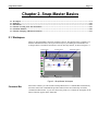
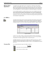
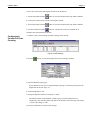
2.1. Workspace ...........................................................................................................................................2-1
Command Bar .......................................................................................................................................2-1
Status Bar..............................................................................................................................................2-2
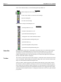
Toolbox .................................................................................................................................................2-2
Instrument Window ...............................................................................................................................2-3
Comment Field......................................................................................................................................2-3
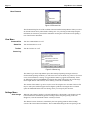
File Menu ..............................................................................................................................................2-4
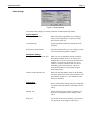
Element Menu .......................................................................................................................................2-4
View Menu............................................................................................................................................2-6
Settings Menu........................................................................................................................................2-6
Start! Menu ...........................................................................................................................................2-9
Window Menu.......................................................................................................................................2-9
Help Menu.............................................................................................................................................2-9
Page ii
Snap-Master User's Manual
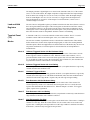
2.2. Elements............................................................................................................................................. 2-10
Overview of Elements..........................................................................................................................2-10
Input Elements .................................................................................................................................... 2-11
Analysis Elements ...............................................................................................................................2-11
Output Elements.................................................................................................................................. 2-12
Menus And Command Bar .................................................................................................................. 2-12
File Menu ............................................................................................................................................ 2-13
Edit Menu ........................................................................................................................................... 2-14
View Menu.......................................................................................................................................... 2-14
2.3. Instruments ........................................................................................................................................ 2-15
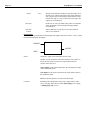
Instrument Construction Guidelines..................................................................................................... 2-15
Frame Characteristics .......................................................................................................................... 2-16
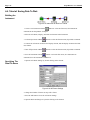
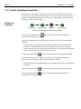
2.4. Tutorial: Creating Your First Instrument ........................................................................................2-16
Creating a New Instrument.................................................................................................................. 2-17
Placing and Connecting the Elements .................................................................................................. 2-18
Running the Instrument ....................................................................................................................... 2-19
2.5. A/D Demo Element ............................................................................................................................ 2-20
A/D Demo Settings.............................................................................................................................. 2-20
2.6. Tutorial: Changing A/D Demo Parameters.......................................................................................2-21
Changing the Sample Rate................................................................................................................... 2-21
Changing the Frame Length ................................................................................................................ 2-22
Stopping the Instrument Automatically................................................................................................ 2-22
Running the Instrument ....................................................................................................................... 2-22
Chapter 3. Display
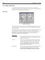
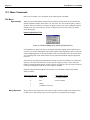
3.1. Display Window...................................................................................................................................3-1
Command Bar .......................................................................................................................................3-2
Scroll Bar ..............................................................................................................................................3-2
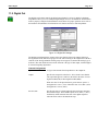
3.2. Plot Types.............................................................................................................................................3-3
Default Plot Templates ..........................................................................................................................3-3
Y vs. T Plots..........................................................................................................................................3-3
Strip Charts ...........................................................................................................................................3-9
Frequency Plots (Mag vs. F, Phase vs. F) ...............................................................................................3-9
Y vs. X, Scatter Plots .............................................................................................................................3-9
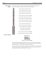
Digital Meters...................................................................................................................................... 3-10
Indicators ............................................................................................................................................ 3-12
Bar Meters........................................................................................................................................... 3-12
Dial Meters.......................................................................................................................................... 3-14
Histogram Plots ................................................................................................................................... 3-15
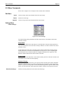
3.3. Menu Commands ...............................................................................................................................3-16
File Menu ............................................................................................................................................ 3-16
Edit Menu ........................................................................................................................................... 3-17
View Menu.......................................................................................................................................... 3-17
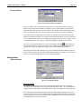
Settings Menu...................................................................................................................................... 3-20
Start Menu........................................................................................................................................... 3-22
Layout Menu ....................................................................................................................................... 3-23
Cursor Menu ....................................................................................................................................... 3-25
Table of Contents
Page iii
3.4. Tutorial: Changing the Display Settings ...........................................................................................3-28
Changing Line Colors and Styles......................................................................................................... 3-28
Deleting and Inserting Plots................................................................................................................. 3-30
Overplotting Multiple Channels........................................................................................................... 3-31
Strip-Charts and Y-X Plots.................................................................................................................. 3-32
Changing Other Plot Components ....................................................................................................... 3-34
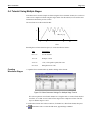
3.5. Tutorial: Using Display Pages ...........................................................................................................3-36
Moving a Plot To A New Display Page ................................................................................................3-36
Changing The Display Page Title ........................................................................................................ 3-36
Changing The Display Page Rows and Columns.................................................................................. 3-37
Running the Instrument ....................................................................................................................... 3-37
3.6. Tutorial: Using Cursors And Markers..............................................................................................3-38
Placing A Cursor ................................................................................................................................. 3-38
Moving The Cursor ............................................................................................................................. 3-39
Finding The Slope Between Two Points...............................................................................................3-39
Using Linked Cursors ..........................................................................................................................3-40
Chapter 4. Disk I/O
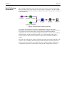
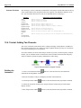
4.1. Data File Overview ..............................................................................................................................4-1
Native Data Files ...................................................................................................................................4-2
Generic Data Files .................................................................................................................................4-2
Data File Naming Conventions..............................................................................................................4-3
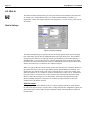
4.2. Disk In..................................................................................................................................................4-4
Disk In Settings .....................................................................................................................................4-4
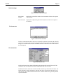
4.3. Disk Out ...............................................................................................................................................4-8
Disk Out Settings...................................................................................................................................4-8
Overwriting Data Files ........................................................................................................................ 4-11
4.4. Tutorial: Saving Data To Disk...........................................................................................................4-12
Building the Instrument....................................................................................................................... 4-12
Specifying The Data File Name ...........................................................................................................4-12
Running The Instrument...................................................................................................................... 4-13
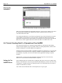
4.5. Tutorial: Reading Data From Disk ...................................................................................................4-14
Building the Instrument....................................................................................................................... 4-14
Specifying The Data File Name ...........................................................................................................4-14
Running The Instrument...................................................................................................................... 4-15
4.6. Data File Formats .............................................................................................................................. 4-15
Data File Structure............................................................................................................................... 4-15
Header Information.............................................................................................................................. 4-15
Exponential Data File Format.............................................................................................................. 4-17
Standard Binary Data File Format ....................................................................................................... 4-19
Fast Binary Data File Format............................................................................................................... 4-20
Comma Separated Variable Data File Format ...................................................................................... 4-21
ASCII Plotter Data File Format ........................................................................................................... 4-21
Binary Plotter Data File Format ........................................................................................................... 4-22
Page iv
Snap-Master User's Manual
Chapter 5. Wave Generator
Command Bar .......................................................................................................................................5-1
Table Columns ......................................................................................................................................5-2
5.1. Waveforms ...........................................................................................................................................5-2
Amplitude Modulation...........................................................................................................................5-3
Bessel ....................................................................................................................................................5-3
Constant ................................................................................................................................................5-4
Cosine And Sine....................................................................................................................................5-4
Frequency Modulation ...........................................................................................................................5-5
Ramp.....................................................................................................................................................5-5
Sawtooth................................................................................................................................................5-6
Sinc .....................................................................................................................................................5-6
Square ...................................................................................................................................................5-7
Trapezoid ..............................................................................................................................................5-7
Triangle.................................................................................................................................................5-8
White Noise...........................................................................................................................................5-8
5.2. Menu Commands .................................................................................................................................5-9
Edit Menu .............................................................................................................................................5-9
Settings Menu........................................................................................................................................5-9
5.3. Tutorial: Creating A Sine Wave........................................................................................................5-10
Building the Instrument....................................................................................................................... 5-10
Setting Up A Waveform.......................................................................................................................5-11
Running the Instrument ....................................................................................................................... 5-12
5.4. Tutorial: Using Multiple Stages ........................................................................................................5-13
Creating Waveform Stages ..................................................................................................................5-13
Configuring Each Waveform Stage......................................................................................................5-14
Running the Instrument ....................................................................................................................... 5-16
Chapter 6. Dynamic Data Exchange
Clipboard...............................................................................................................................................6-1
Dynamic Data Exchange (DDE) ............................................................................................................6-1
DDE And Snap-Master..........................................................................................................................6-3
DDE And Other Applications ................................................................................................................6-5
6.1. DDE In .................................................................................................................................................6-5
Command Bar .......................................................................................................................................6-5
Table Columns ......................................................................................................................................6-6
Menu Commands ..................................................................................................................................6-6
Settings Menu........................................................................................................................................6-7
6.2. DDE Out...............................................................................................................................................6-8
6.3. Tutorial: Receiving Data In From A Local Spreadsheet .................................................................. 6-11
Building the Instrument....................................................................................................................... 6-11
Configuring the DDE Conversation ..................................................................................................... 6-12
Setting The DDE In Frame Settings..................................................................................................... 6-12
Setting Up The DDE In Channel ......................................................................................................... 6-13
Running the Instrument ....................................................................................................................... 6-14
6.4. Tutorial: Sending Data Out To A Local Spreadsheet.......................................................................6-14
Building the Instrument....................................................................................................................... 6-14
Configuring the A/D Demo.................................................................................................................. 6-15
Copying the DDE Link ........................................................................................................................6-15
Running the Instrument ....................................................................................................................... 6-16
Table of Contents
Page v
6.5. Tutorial: Using Block Mode ..............................................................................................................6-17
Modifying the Instrument .................................................................................................................... 6-17
Copying a DDE Data Block .................................................................................................................6-17
Running the Instrument ....................................................................................................................... 6-18
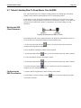
6.6. Tutorial: Sending Data To A Spreadsheet Over NetDDE ................................................................ 6-18
Setting Up The NetDDE Server ...........................................................................................................6-18
Setting Up The NetDDE Client............................................................................................................ 6-20
Running the Instrument ....................................................................................................................... 6-20
6.7. Tutorial: Sending Data To Snap-Master Over NetDDE................................................................... 6-21
Building the DDE Client Instrument.................................................................................................... 6-21
Configuring the DDE Conversation ..................................................................................................... 6-21
Setting Up The DDE In Channels........................................................................................................ 6-22
Running the Instrument ....................................................................................................................... 6-22
Data Acquisition
Chapter 7. Sensors & Signal Conditioning
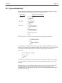
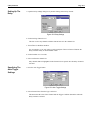
7.1. Sensor Database...................................................................................................................................7-1
Sensor Database Files ............................................................................................................................7-2
Input And Output Values And Units......................................................................................................7-2
Sensor Assignments...............................................................................................................................7-3
Table Columns ......................................................................................................................................7-3
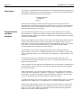
7.2. Sensor Menu Commands .....................................................................................................................7-4
View Menu............................................................................................................................................7-4
Settings Menu........................................................................................................................................7-4
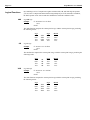
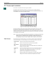
7.3. Signal Conditioning .............................................................................................................................7-7
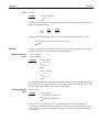
7.4. Tutorial: Adding A Sensor To The Sensor Database..........................................................................7-8
Building the Instrument.........................................................................................................................7-8
Inserting A New Sensor .........................................................................................................................7-8
7.5. Tutorial: Using The Sensor Element .................................................................................................7-10
Building The Instrument...................................................................................................................... 7-10
Assigning a Sensor To An Input Channel ............................................................................................ 7-11
Running The Instrument...................................................................................................................... 7-11
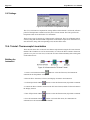
7.6. Tutorial: Updating a Sensor's Calibration History ..........................................................................7-12
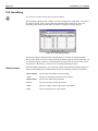
7.7. Tutorial: Additional Sensor Database Hints .....................................................................................7-13
Copying An Existing Sensor................................................................................................................ 7-13
Using The Sensor To Assign Channel Labels....................................................................................... 7-13
Chapter 8. Data Acquisition
8.1. Analog Input (A/D) ..............................................................................................................................8-1
Command Bar .......................................................................................................................................8-2
Table Columns ......................................................................................................................................8-2
Dialog Interface.....................................................................................................................................8-3
8.2. Menu Commands .................................................................................................................................8-4
Edit Menu .............................................................................................................................................8-4
Settings Menu........................................................................................................................................8-4
Device Menu ....................................................................................................................................... 8-11
8.3. Digital In ............................................................................................................................................ 8-13
Digital In Settings ............................................................................................................................... 8-13
Page vi
Snap-Master User's Manual
8.4. Tutorial: Acquiring Analog Data ......................................................................................................8-13
Building the Instrument....................................................................................................................... 8-13
Configuring the A/D Element.............................................................................................................. 8-14
Running the Instrument ....................................................................................................................... 8-15
8.5. Tutorial: Using Triggers to Start Acquisition...................................................................................8-15
Setting Up A Trigger ........................................................................................................................... 8-15
Running the Instrument ....................................................................................................................... 8-16
8.6. Tutorial: Acquiring From Multiple Devices .....................................................................................8-17
Building the Instrument....................................................................................................................... 8-17
Configuring the Input Elements........................................................................................................... 8-18
Saving Data From Only One Channel.................................................................................................. 8-20
Running The Instrument...................................................................................................................... 8-20
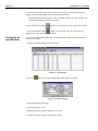
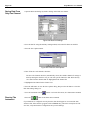
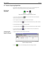
8.7. Tutorial: Acquiring Digital Data.......................................................................................................8-21
Building the Instrument....................................................................................................................... 8-21
Configuring the Digital In Element ..................................................................................................... 8-21
Running the Instrument ....................................................................................................................... 8-22
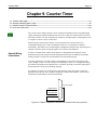
Chapter 9. Counter Timer
Special Wiring Instructions ...................................................................................................................9-1
9.1. Counter Timer Input ...........................................................................................................................9-2
9513 Setup.............................................................................................................................................9-2
9.2. Tutorial: Measuring Pulse Counts.......................................................................................................9-6
Building the Instrument.........................................................................................................................9-6
Configuring A Counter For Pulse Counting ...........................................................................................9-7
Configuring A Counter As An Internal Pacer ........................................................................................9-9
Signal Connections................................................................................................................................9-9
Running The Instrument...................................................................................................................... 9-10
9.3. Tutorial: Frequency Measurements ..................................................................................................9-10
Configuring A Counter To Measure Frequency....................................................................................9-10
Signal Connections.............................................................................................................................. 9-11
Running The Instrument...................................................................................................................... 9-12
Alternate Frequency Measurement Method ..........................................................................................9-12
9.4. Overview Of The 9513....................................................................................................................... 9-14
Source, Gate, and Output..................................................................................................................... 9-14
Load and Hold Registers......................................................................................................................9-15
Terminal Count (T/C).......................................................................................................................... 9-15
Modes.................................................................................................................................................. 9-15
Chapter 10. RS-232
Answers To Commonly Asked Questions.............................................................................................10-1
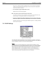
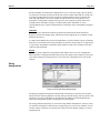
10.1. RS-232 Settings ................................................................................................................................ 10-2
String Assignments ............................................................................................................................. 10-3
Configuration ...................................................................................................................................... 10-7
10.2. Tutorial: Writing Example RS-232 Strings ....................................................................................10-8
Table of Contents
Page vii
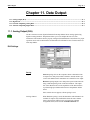
Chapter 11. Data Output
11.1. Analog Output (D/A)........................................................................................................................11-1
D/A Settings........................................................................................................................................ 11-1
11.2. Digital Out........................................................................................................................................ 11-3
11.3. Tutorial: Outputting Analog Data...................................................................................................11-4
Building the Instrument....................................................................................................................... 11-4
Configuring the A/D Demo.................................................................................................................. 11-5
Configuring the A/D Hardware............................................................................................................ 11-5
Configuring the D/A............................................................................................................................ 11-6
Running the Instrument ....................................................................................................................... 11-7
11.4. Tutorial: Outputting Digital Data ...................................................................................................11-7
Building the Instrument....................................................................................................................... 11-7
Configuring the Digital Out Element ................................................................................................... 11-8
Running the Instrument ....................................................................................................................... 11-8
Data Analysis
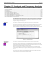
Chapter 12. Analysis and Frequency Analysis
Analysis............................................................................................................................................... 12-1
Frequency Analysis.............................................................................................................................. 12-1
Command Bar ..................................................................................................................................... 12-2
Table Columns .................................................................................................................................... 12-2
Quick Function Reference....................................................................................................................12-3
12.1. Menu Commands ............................................................................................................................. 12-4
File Menu ............................................................................................................................................ 12-4
Builder Menu ...................................................................................................................................... 12-5
Settings Menu...................................................................................................................................... 12-7
12.2. Functions ........................................................................................................................................ 12-11
Arithmetic Functions ......................................................................................................................... 12-12
Trigonometric Functions.................................................................................................................... 12-13
Calculus Functions ............................................................................................................................ 12-15
Statistical Functions........................................................................................................................... 12-16
Logical Functions .............................................................................................................................. 12-18
Filters ................................................................................................................................................ 12-20
Time Functions.................................................................................................................................. 12-22
Data Ranges ...................................................................................................................................... 12-22
Miscellaneous Functions.................................................................................................................... 12-25
12.3. Equation Syntax ............................................................................................................................. 12-26
Equation Format................................................................................................................................ 12-27
User Defined Functions ..................................................................................................................... 12-27
12.4. Tutorial: Adding Two Channels.................................................................................................... 12-28
Building the Instrument..................................................................................................................... 12-28
Building The Equation ...................................................................................................................... 12-29
Running the Instrument ..................................................................................................................... 12-31
12.5. Tutorial: Performing A Block Average......................................................................................... 12-32
Building The Equation ...................................................................................................................... 12-32
Running The Instrument.................................................................................................................... 12-34
12.6. Tutorial: Finding When An Event Occurs.................................................................................... 12-34
Building The Equation ...................................................................................................................... 12-34
Running The Instrument.................................................................................................................... 12-36
Page viii
Snap-Master User's Manual
12.7. Tutorial: Integrating Over A Specific Range Of Data ................................................................. 12-37
Building The Equation ...................................................................................................................... 12-37
Running The Instrument.................................................................................................................... 12-39
12.8. Tutorial: Defining Your Own Functions ....................................................................................... 12-40
Defining A New Function.................................................................................................................. 12-40
Calling The Function In An Equation................................................................................................ 12-41
Running the Instrument ..................................................................................................................... 12-42
Chapter 13. Command
Command Bar ..................................................................................................................................... 13-1
Equation Table Columns ..................................................................................................................... 13-1
13.1. Menu Commands ............................................................................................................................. 13-2
View ................................................................................................................................................... 13-2
Settings ............................................................................................................................................... 13-2
13.2. Command Equations........................................................................................................................13-3
Subroutines.......................................................................................................................................... 13-4
Result Channels and State Variables.................................................................................................... 13-4
Comparisons........................................................................................................................................ 13-5
Logical Functions ................................................................................................................................ 13-6
Actions ................................................................................................................................................ 13-7
Case Statements................................................................................................................................... 13-9
13.3. Tutorial: Creating A Trigger To Stop.............................................................................................13-9
Building the Instrument....................................................................................................................... 13-9
Writing A Command Routine ............................................................................................................ 13-10
Turning Off Status Messages For The Instrument .............................................................................. 13-11
Running The Instrument.................................................................................................................... 13-11
13.4. Tutorial: Subroutines and State Variables.................................................................................... 13-12
Defining The Equation Table............................................................................................................. 13-12
Running The Instrument.................................................................................................................... 13-14
13.5. Tutorial: Automatically Starting Another Instrument ................................................................. 13-15
Building the Second Instrument......................................................................................................... 13-15
Updating The Command Routine....................................................................................................... 13-16
Running The Instrument.................................................................................................................... 13-16
Chapter 14. FFT
Command Bar ..................................................................................................................................... 14-1
Table Columns .................................................................................................................................... 14-1
14.1. Menu Commands ............................................................................................................................. 14-3
Builder ................................................................................................................................................ 14-3
Settings ............................................................................................................................................... 14-5
14.2. Functions .......................................................................................................................................... 14-6
Summary ............................................................................................................................................. 14-6
Forward FFT ....................................................................................................................................... 14-7
Inverse FFT ......................................................................................................................................... 14-7
Auto Power Spectrum ..........................................................................................................................14-7
Auto Power Spectral Density ...............................................................................................................14-7
Cross Power Spectrum .........................................................................................................................14-8
Cross Power Spectral Density ..............................................................................................................14-8
Coherence Function............................................................................................................................. 14-8
Coherent Output Power........................................................................................................................14-9
Transfer Function ................................................................................................................................ 14-9
Table of Contents
Page ix
Compliance ....................................................................................................................................... 14-10
Impedance ......................................................................................................................................... 14-10
Dynamic Compressibility................................................................................................................... 14-10
Bulk Modulus .................................................................................................................................... 14-10
Admittance........................................................................................................................................ 14-10
Dynamic Flexibility ........................................................................................................................... 14-10
Mobility............................................................................................................................................. 14-11
Dynamic Accelerance ........................................................................................................................ 14-11
Dynamic Stiffness.............................................................................................................................. 14-11
Transmissibility ................................................................................................................................. 14-11
Dynamic Inertia................................................................................................................................. 14-11
14.3. Window Types................................................................................................................................ 14-11
Selecting A Window Type ................................................................................................................. 14-12
Window Width Response................................................................................................................... 14-13
Window Effects Illustrated................................................................................................................. 14-14
Blackman .......................................................................................................................................... 14-16
Blackman-Harris ............................................................................................................................... 14-17
Bohman............................................................................................................................................. 14-17
Cauchy .............................................................................................................................................. 14-17
Cosine 4th Power............................................................................................................................... 14-18
Cosine Tapered.................................................................................................................................. 14-18
Exact Blackman................................................................................................................................. 14-18
Exponential ....................................................................................................................................... 14-19
Extended Cosine Bell......................................................................................................................... 14-19
Flat Top............................................................................................................................................. 14-20
Gaussian............................................................................................................................................ 14-20
Half Cycle Sine.................................................................................................................................. 14-20
Hamming .......................................................................................................................................... 14-21
Hann ................................................................................................................................................. 14-21
Hanning-Poisson ............................................................................................................................... 14-21
Kaiser-Bessel..................................................................................................................................... 14-22
Parabolic ........................................................................................................................................... 14-22
Parzen ............................................................................................................................................... 14-22
Poisson .............................................................................................................................................. 14-23
Rectangular ....................................................................................................................................... 14-23
Riemann ............................................................................................................................................ 14-23
Sine 3rd Power .................................................................................................................................. 14-24
Triangular ......................................................................................................................................... 14-24
14.4. Window Width............................................................................................................................... 14-24
Available Widths ............................................................................................................................... 14-25
Frequency Resolution and Spectral Lines ........................................................................................... 14-25
Forcing Periodicity ............................................................................................................................ 14-25
14.5. Tutorial: Performing a Forward FFT ........................................................................................... 14-26
Building the Instrument..................................................................................................................... 14-26
Configuring the A/D Demo Element.................................................................................................. 14-27
Calculating The Forward FFT............................................................................................................ 14-27
Running The Instrument.................................................................................................................... 14-29
14.6. Tutorial: Performing an Inverse FFT ........................................................................................... 14-29
Calculating An Inverse FFT............................................................................................................... 14-29
Running the Instrument ..................................................................................................................... 14-31
14.7. Tutorial: Cross Power Spectrum ................................................................................................... 14-31
Adding The Second A/D Demo ......................................................................................................... 14-31
Calculating the Cross Power Spectrum .............................................................................................. 14-32
Running the Instrument ..................................................................................................................... 14-33
Page x
Snap-Master User's Manual
14.8. Tutorial: Transfer and Coherence Functions ............................................................................... 14-34
Calculating The Transfer Function .................................................................................................... 14-34
Calculating The Coherence Function ................................................................................................. 14-35
Running the Instrument ..................................................................................................................... 14-36
Chapter 15. Utility Elements
15.1. Relay................................................................................................................................................. 15-1
Auto Toggle Settings ...........................................................................................................................15-2
15.2. Tutorial: Relay................................................................................................................................. 15-4
Building the Instrument....................................................................................................................... 15-4
Configuring The Wave Generator........................................................................................................ 15-4
Setting Up The Relay...........................................................................................................................15-5
Specifying The Auto Toggle Settings...................................................................................................15-5
Running the Instrument ....................................................................................................................... 15-6
15.3. Thermocouple Linearization ...........................................................................................................15-7
Table Columns .................................................................................................................................... 15-7
CJC Settings........................................................................................................................................ 15-8
15.4. Tutorial: Thermocouple Linearization............................................................................................15-8
Building the Instrument....................................................................................................................... 15-8
Configuring The Wave Generator........................................................................................................ 15-9
Linearizing Thermocouple Channels ................................................................................................. 15-10
Specifying The CJC Settings.............................................................................................................. 15-11
Running the Instrument ..................................................................................................................... 15-11
15.5. Smoothing....................................................................................................................................... 15-12
Table Columns .................................................................................................................................. 15-12
Smoothing Options............................................................................................................................ 15-13
15.6. Tutorial: Smoothing....................................................................................................................... 15-13
Building the Instrument..................................................................................................................... 15-13
Configuring The Wave Generator...................................................................................................... 15-14
Configuring The Smoothing Element ................................................................................................ 15-15
Specifying The Rise Time.................................................................................................................. 15-16
Running the Instrument ..................................................................................................................... 15-16
15.7. Histogram....................................................................................................................................... 15-17
Histogram.......................................................................................................................................... 15-18
Band Analysis ................................................................................................................................... 15-18
Octave Band Analysis........................................................................................................................ 15-18
15.8. Tutorial: Histogram ....................................................................................................................... 15-19
Building the Instrument..................................................................................................................... 15-19
Performing A Histogram Calculation................................................................................................. 15-19
Running the Instrument ..................................................................................................................... 15-21
15.9. MultiFrame .................................................................................................................................... 15-22
15.10. Tutorial: MultiFrame .................................................................................................................. 15-22
Building the Instrument..................................................................................................................... 15-22
Summing Five Frames Into One Frame.............................................................................................. 15-23
Running the Instrument ..................................................................................................................... 15-25
Outputting All Five Frames ............................................................................................................... 15-25
Table of Contents
Page xi
FactorySuite
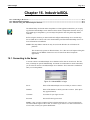
Chapter 16. IndustrialSQL
16.1. Connecting to the Server .................................................................................................................16-1
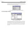
16.2. IndustrialSQL In Settings................................................................................................................16-2
Time Controls and Resolution..............................................................................................................16-3
Tree View............................................................................................................................................ 16-3
Active Tags ......................................................................................................................................... 16-3
16.3. Tutorial: Using The IndustrialSQL In Element..............................................................................16-4
Building the Instrument....................................................................................................................... 16-4
Connecting to the IndustrialSQL Server Database................................................................................ 16-4
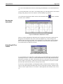
Activating Tags ................................................................................................................................... 16-5
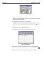
Selecting the Start and End Dates ........................................................................................................ 16-5
Setting the Resolution..........................................................................................................................16-6
Running the Instrument ....................................................................................................................... 16-6
Appendices
Appendix A. Glossary
A-1
Appendix B. Bibliography
B-1
Appendix C. Aliasing
C-1
Appendix D. DDE Commands and Parameters
D-1
Appendix E. PC Computer Information
E-1
Appendix X. Index
X-1
Getting Started
Page 1-1
Chapter 1. Getting Started
1.1. Welcome! .................................................................................................................................................................... 1-1
1.2. Technical Support....................................................................................................................................................... 1-3
1.3. System Requirements ................................................................................................................................................. 1-5
1.4. Installing Snap-Master ............................................................................................................................................... 1-6
1.5. Computer Configuration ............................................................................................................................................ 1-6
1.6. Start Using Snap-Master ............................................................................................................................................ 1-8
1.1. Welcome!
Congratulations on purchasing Snap-Master for Windows - the new generation of PC-based data
acquisition, analysis, control, and display software from HEM Data Corporation. Snap-Master
combines advanced data acquisition and storage capabilities with time and frequency domain
analysis and near real-time plotting, all without programming! From high speed data acquisition,
display and storage to monitoring and control, Snap-Master has the power to meet the needs of a
wide variety of applications.
Snap-Master is divided into three modules: Data Acquisition (SM-DA), Waveform Analyzer
(SM-WA, formerly known as General Analysis), and Frequency Analyzer (SM-FA). Each is a
fully functional stand-alone package that includes data display, storage, retrieval, and Dynamic
Data Exchange (DDE) capabilities. By integrating the different Snap-Master modules you can
create a complete software solution to meet your total needs.
NOTE: Some chapters and tutorials may contain additional features not included in your SnapMaster software. For more information on how to obtain these additional features, please
contact the vendor from whom you purchased Snap-Master.
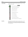
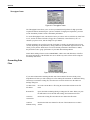
Sample
Instruments
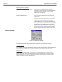
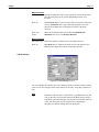
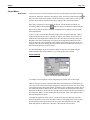
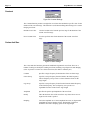
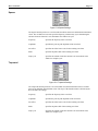
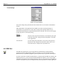
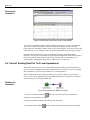
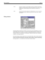
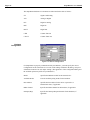
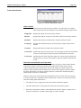
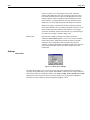
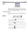
Included with Snap-Master are sample instruments that demonstrate different features of the
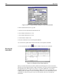
program. To open these files, run Snap-Master then select the File menu, Open Instrument
command. The Open dialog box will appear with a list of the Instrument files that you can use.
Try using the Viewer button in the Open dialog to see the contents of each instrument.
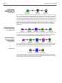
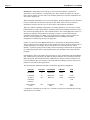
In addition to the instruments included on disk, the following instruments represent the SnapMaster equivalents for many pieces of conventional equipment. It is highly recommended that
you complete the Basic Tutorials before you attempt to employ these examples. Once you have
become comfortable with Snap-Master, this section can be used as a reference guide to
conventional test systems and their equivalent in Snap-Master.
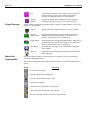
Data Acquisition
System
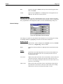
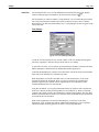
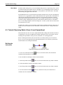
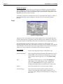
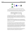
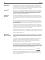
This instrument is representative of a system that will acquire real world data and store it to a
disk. An analog input signal is sampled by an A/D (with all sampling parameters specified and
maintained by Snap-Master), and the data is stored to a file on a disk. By using Snap-Master's
Fast Binary Data Format, you can stream the data to disk at high sampling rates.
Page 1-2
Snap-Master User's Manual
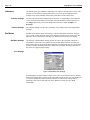
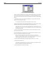
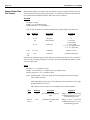
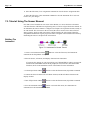
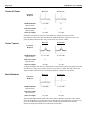
Digital Storage
Oscilloscope, Strip
Chart Recorder, Y-X
Plotter, Meter
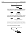
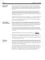
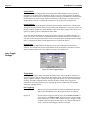
This instrument is similar to the Data Acquisition System but in addition to sending the data to a
disk, it is also displayed on the computer monitor. The difference between each of the instrument
samples is how the Display element graphs the data. The Digital Storage Oscilloscope emulates
an oscilloscope by plotting from right to left against a stationary set of axes and using time as the
X-axis. The Strip Chart Recorder is similar, but both the axes and the data scroll continuously
from right to left. The Y-X Plotter uses the same configuration as the Oscilloscope but the X-axis
is now referenced against one of the input channels, not as a function of time. To emulate a
portable volt meter, the Display element plots the numeric data values using the Digital Meter
display type.
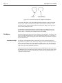
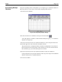
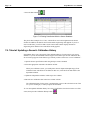
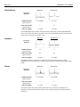
Waveform Generator,
Controller, Monitoring
and Diagnostics
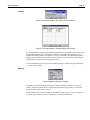
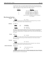
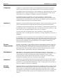
The important feature about this instrument is its ability to output both analog and digital signals
according to the system's input signal. The input data is analyzed and monitored, resulting in
automatic decision making that will initialize subsequent actions for the test system.
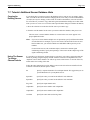
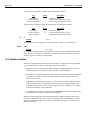
Waveform Analyzer,
Spectrum Analyzer,
Signal Analyzer,
Digital Filter
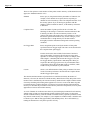
This Instrument configuration allows for analysis and manipulation of data in the digital domain.
The Analysis element uses digital filtering to remove unwanted noise from the signal, and the
FFT element performs a Fourier analysis on both the original and the filtered signals.
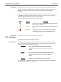
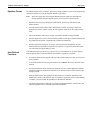
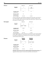
PID Control
This instrument configuration allows for PID (proportional, integral, differential) Control. The
A/D is used to acquire the incoming data, the Analysis element calculates the Error and the PID
output equations, then outputs a value using the D/A element.
Getting Started
Page 1-3
1.2. Technical Support
Registration
Please take the time to fill out and return the Registration Card as directed. Along with
information on your software use and needs, the data you provide helps us to serve you more
efficiently if you require technical support.
Please be sure to read the Software License Agreement for any warranty and disclaimer
information regarding the use of this product.
Customer Support
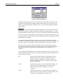
Unless otherwise warranted by your vendor, registering your software entitles you to basic
customer support coverage of :
•
Free telephone support for four (4) months from date of purchase (duration of support period
may vary according to whom you purchased this product from)
•
Free product upgrades for thirty (30) days from date of purchase
An Extended Support Program (ESP) for continued technical support and software upgrades can
be purchased after the standard support policy expires. Please contact an HEM Data sales
representative for more information.
If you purchased the software from a third-party reseller, your Customer Support terms
(including extended support) may differ. Please contact the company you purchased the software
from for further information.
HEM Data reserves the right to withhold customer support service at any time from unregistered
users or from anyone who abuses the service. We also reserve the right to change the support fee
structure, support policies, and procedures without notice.
Where To Go For
Help
To save time, please refer to the applicable software and hardware documentation before calling
technical support. Our manuals are designed to provide answers to the questions most commonly
asked about the program.
If you have access to the World Wide Web, check out http://www.hemdata.com which contains a
section with Application Notes with advanced uses of Snap-Master as well special hints and
tricks.
If you purchased the software directly from HEM Data, you may call our Technical Support Staff
at (248) 559-5607. Technical Support hours are between 8:00 AM and 5:00 PM (Eastern Time
Zone). Or, you can fax us your questions 24 hours a day at (248) 559-8008. Faxing technical
support questions is preferred since it is an efficient way to define and illustrate situations or
problems. This also allows the support staff time to research the problem before contacting you
with solutions.
If you purchased the software through a third party, contact them directly for technical support.
Page 1-4
When You Call For
Support
Snap-Master User's Manual
Please register your software before calling for technical support. You may be asked to fax in
your registration card if you have not already registered.
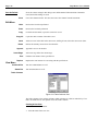
The amount of information needed depends upon the complexity of your question. Minimal
information generally required for efficient technical support includes:
•
Version and build numbers from the Help menu, About Snap-Master dialog box or the SnapMaster installation disks
•
System information from the Help menu, About Snap-Master dialog box
•
Serial numbers from the Snap-Master installation disks
If at all possible, you should have immediate access to your computer and Snap-Master while you
are calling. This helps the technical support representative quickly determine if a proposed
solution is valid, as well as gather additional information as needed.
You may be asked to send additional information to help us assist you such as copies of the SnapMaster instrument files, data files, or photocopies of the original Snap-Master diskettes.
What Is Technical
Support?
As indicated previously, technical support for Snap-Master is a service provided by the party
from whom you purchased the software. In combination with the user's manuals for the software
and hardware, technical support is intended to assist you to attain useful operation of SnapMaster.
While not a complete list, the following paragraphs should give you an idea of the services to
expect from HEM Data's Technical Support staff:
•
Answers to General Usability Questions - HEM Data's Technical Support staff will answer
general usability questions, which are defined as non-programming issues including: product
features, menu commands, formatting, and aspects of the user interface (use of the windows,
dialog boxes, etc.). We will also answer general installation questions for both the software
and any I/O hardware sold directly by HEM Data.
•
Resolution of Repeatable Problems - While Snap-Master has endured thousands of hours
of testing and millions of hours of use, there are times when you may encounter a repeatable
problem with the software. When you call technical support with a description of the
problem, please have a complete description of the problem and related circumstances
(which means that more information than "Snap-Master crashes when I run it" is required).
You may be asked for copies of the instrument, data, or configuration files for Snap-Master,
and for the sequence of events leading up to the problem (including anything that has
changed since the instrument last ran successfully). Whenever practical, HEM Data will
assist in the timely resolution of such problems. However, the only way we can fix such a
problem is if we can duplicate it. Your assistance in this area is greatly appreciated.
•
Application and Instrument Design Is NOT Included - HEM Data's technical support
service does not include the detailed applying of Snap-Master to the design of a customer's
specific application, support customer written code in any language to access the features or
files created by Snap-Master, or provide support for hardware not sold directly by HEM
Data. For assistance in these areas, contact HEM Data for information on our
consulting/engineering services.
Getting Started
Page 1-5
Because your contact point for technical support is the company you purchased the software from,
these technical support services may differ from HEM Data's. Please contact your software
vendor for more information on the technical support services they provide.
Extended Support
Programs
HEM Data offers a valuable extended support program (ESP) which increases the period of
technical support and product maintenance for yearly periods beyond the initial four months.
Like our software, our extended support program is designed to focus on our customers' changing
requirements. For the duration selected, the Extended Support Program includes:
• General support by telephone and fax
• Assistance in problem diagnosis and resolution
• Free minor software upgrades ("builds"), when available, to correct a customer's
problem
or provides needed functional enhancement. Upgrades distributed via either our World
Wide Web page (http://www.hemdata.com) or by snail mail
• Automatic free upgrades to major software upgrades (i.e. from 3.2 to 3.3 or 4.0) released
during the support period
• A subscription to our technical newsletter
• Discounts on training, seminars, and engineering consultation
The price of an Extended Support Programs depends on the software module(s) and period
covered. You must be a registered user and own the current version of the software to enroll in a
support program. You may have to pay an upgrade fee to bring your product up to the current
version level. Please contact HEM Data for current pricing or if you need more information.
1.3. System Requirements
In order to use this product, you will need the following hardware and software:
•
Windows 3.1 or higher
•
A computer which runs Windows in 386 Enhanced mode (386 or greater)
•
5-7 MB free hard disk space (plus space for data files)
•
4 MB RAM (8 MB recommended)
•
Mouse or other pointing device
•
For high speed plotting a local bus graphics accelerator is recommended
•
For high speed data analysis, a math coprocessor is recommended
Page 1-6
Snap-Master User's Manual
1.4. Installing Snap-Master
Snap-Master's installation program is used for both new installations and upgrades to existing
installations. To install or upgrade Snap-Master, follow these instructions:
•
Insert Disk 1 of the most recent Snap-Master module you received (for example, Disk 1 of
the Data Acquisition module)
•
In Program Manager, select the File menu, Run command (for Windows 95 users, select the
Start button, Run command)
•
Type a:setup in the command line (use the floppy disk drive letter you are installing from),
then press the OK button
•
When you reach the screen that specifies the destination path for Snap-Master, type the hard
disk directory where you want to install the program (the default is C:\SM). If you are
performing an upgrade, type the directory where Snap-Master is already installed
•
When you reach the screen that lists the installation or upgrade options, select the check
boxes of the Snap-Master modules you are going to install or upgrade.
•
Follow the instructions on screen and insert the correct diskettes as the installation program
asks for them. The installation program will add an icon for the latest installation of SnapMaster. When installation is completed, double click on the new icon to start the program.
1.5. Computer Configuration
Snap-Master operates under Microsoft Windows 3.1. If you are using Windows 3.0, you must
upgrade to Windows 3.1 before you can run Snap-Master.
The About Snap-Master dialog box contains information about Snap-Master and the support
libraries, as well as information about your computer. This information can be recalled at any
time from the Snap-Master workspace with the Help menu, About Snap-Master command.
Windows 3.1
After Snap-Master is installed, you may need to check the CONFIG.SYS and AUTOEXEC.BAT
files (located in the root directory of your startup drive). If any of these files are found, please
read the following information for further details.
HIMEM.SYS
This is the extended manager program distributed with MS-DOS and
Windows. All Windows programs use extended memory to access the
memory above 640 KB. Therefore, Snap-Master is designed to work with
HIMEM.SYS. Make sure that the following line is contained in the
CONFIG.SYS file (substitute the directory where your copy of HIMEM.SYS
is stored): DEVICE=C:\WINDOWS\HIMEM.SYS.
EMM386.EXE
QEMM.SYS
386MAX.SYS
This program emulates expanded memory using the installed extended
memory. Some non-Windows applications use expanded memory, but all
Windows programs use extended memory. If you encounter problems with
data acquisition, try removing all expanded memory emulation programs
from the CONFIG.SYS file. For more information about extended and
expanded memory, refer to your DOS or Windows manuals.
Getting Started
Page 1-7
SHARE.EXE
If you have installed the Data Acquisition Module, you may need to install
SHARE (which comes with DOS) in order for the Sensor database to operate
correctly. If you receive the error message "Is SHARE loaded?" when adding
a Sensor element to the instrument, add the following command to your
CONFIG.SYS (substitute the directory where your copy of SHARE.EXE is
stored): INSTALL=C:\DOS\SHARE.EXE
The following CONFIG.SYS and AUTOEXEC.BAT files are the "bare minimum" requirements
for Snap-Master to operate correctly. If you are using other software programs, your routines may
differ slightly. When calling for technical support, you may be asked to either fax a copy of your
CONFIG.SYS and AUTOEXEC.BAT files, or you may be asked to try the following files. For
more information on these commands, refer to your DOS and Windows manuals.
386 Enhanced
Mode
CONFIG.SYS
AUTOEXEC.BAT
DOS=HIGH,UMB
DEVICE=C:\HIMEM.SYS
FILES=30
BUFFERS=30
STACKS=9,256
@ECHO OFF
PROMPT $p$g
PATH=C:\DOS;C:\WINDOWS
Windows 3.1 has two operating modes: Standard Mode and 386 Enhanced Mode. For Windows
3.11 and higher (including Windows for Workgroups), only 386 Enhanced Mode is available. If
you attempt to start Windows in Standard Mode, you will receive an error message.
The major differences between the two modes are how DOS sessions are handled and virtual
memory. In 386 Enhanced Mode you can have multiple DOS sessions running concurrently,
while Standard Mode only allows one DOS session at a time. Also, 386 Enhanced Mode allows
you to use part of the hard drive to emulate RAM using virtual memory.
Because 386 Enhanced Mode allows for multiple “Virtual DOS Machines,” certain tasks operate
more slowly than in Standard Mode. In Snap-Master, this will usually be most evident while
performing high speed data acquisition. If you encounter frequent overruns while acquiring data,
try switching to Standard Mode using the /s command line switch when starting Windows.
When you are using the Data Acquisition Module to acquire data, you must allocate memory for
any I/O hardware which uses DMA (Direct Memory Access) to transfer data from the hardware
to the computer. For hardware that does not use DMA, you do not need to allocate any special
buffers.
In general, any I/O hardware that uses DMA requires a 64 KB (kilobyte) block of memory to
write into. Therefore for each I/O hardware function that uses DMA, you need 64 KB of memory
in the buffer. If you encounter messages in the Status Log telling you that no buffer could be
allocated, you must either increase the size of the buffer or close other instruments in the
workspace that contain DMA hardware elements.
When Windows is running in 386 Enhanced Mode, Snap-Master uses a VxD (Virtual Device
Driver, which is installed automatically with Snap-Master) to allocate a block of memory for
DMA. To set the amount of memory allocated for DMA data transfer, select the Options menu,
then the Global Settings command. Change the setting for # of DMA Boards to the maximum
number of DMA-based I/O hardware devices you will be using simultaneously. You must restart
Windows to have your changes take effect.
Page 1-8
Standard Mode
Snap-Master User's Manual
If you are running Windows 3.10 in Standard Mode, you must run the SMSTART program to
allocate memory for DMA-based data acquisition hardware before running Windows. The
instructions for using the SMSTART program are as follows:
•
If you are currently running Windows, exit Windows. DO NOT use the DOS shell within
Windows to run the SMSTART program.
•
Change to the SM directory where the Snap-Master program resides.
•
Type smstart /x"win /s". Press ENTER.
This command runs the Snap-Master support program and runs Windows in Standard mode.
If Windows does not start, try typing the complete path name of your Windows files before
the win command (for example smstart /x "c:\windows\win /s").
If you include this command in your AUTOEXEC.BAT file, the SMSTART program is
executed and Windows runs in Standard mode each time you start your machine. This
command MUST be in the last line your AUTOEXEC.BAT file.
Another option is to create a batch file that will run SMSTART, Windows in Standard Mode,
and Snap-Master. The batch file might look like this:
cd\sm
smstart /x"c:\windows\win /s sm.exe"
cd\
To allocate more memory for SMSTART, you can include a number (expressed in Kilobytes)
after the SMSTART command (for example, SMSTART 256 allocates 256 KB of memory). By
default, SMSTART allocates 128 KB of memory. For additional information about the
SMSTART program, type smstart /?.
Windows 95
All of Snap-Master's features and capabilities are available when running under Windows 95. All
comments about allocating buffers for data acquisition in the 386 Enhanced Mode section apply
to Windows 95 as well.
Windows NT
Snap-Master operates as a data display and analysis program when running under Windows NT.
The data acquisition features are not available.
Using Disk
Compression or
Caching Software
When using any type of disk compression software (such as DoubleSpace or Stacker), the actual
throughput rate for writing high speed data to disk in the Fast Binary format will decrease. The
actual performance for all data file formats will vary between computers. As a rule of thumb,
avoid writing high speed data to compressed disks.
You should disable any disk caching software (such as SMARTDRV) if you are acquiring data
using the Fast Binary format. SMARTDRV is automatically installed with Windows 3.1, so you
will have to remark this out of AUTOEXEC.BAT before using the FBDF format.
1.6. Start Using Snap-Master
This manual is designed to give you an overview of Snap-Master's components and how they
work together. Many basic examples are provided along the way to help get you started. These
tools will help you construct your more complicated tests in less time using Snap-Master. Enjoy!
Snap-Master Basics
Page 2-1
Chapter 2. Snap-Master Basics
2.1. Workspace .................................................................................................................................................................. 2-1
2.2. Elements.....................................................................................................................................................................2-10
2.3. Instruments ................................................................................................................................................................2-15
2.4. Tutorial: Creating Your First Instrument ................................................................................................................2-16
2.5. A/D Demo Element ....................................................................................................................................................2-20
2.6. Tutorial: Changing A/D Demo Parameters ..............................................................................................................2-21
2.1. Workspace
When you start Snap-Master, the main workspace appears. The function of the workspace is to
hold the instrument windows, and to provide an easy way of building new instruments. The
workspace has its own title bar and menu as well as other key features, as shown in Figure 2-1.
Command Bar
Toolbox
Comment Field
Instrument Window
Status Bar
Figure 2-1 Snap-Master Workspace
Command Bar
Most of the windows you will encounter in Snap-Master have a Command Bar located directly
below the menu. Each Command Bar provides buttons for the most commonly used menu
commands in that window. As you move the mouse pointer over a button, the description of the
button’s function appears in the Status Bar.
Page 2-2
Snap-Master User's Manual
Some of the common buttons you will find throughout Snap-Master are:
Description
Button
Starts and stops the active instrument
Creates a new window or clears the current settings
Opens an existing file
Saves the current settings
Buttons that are unique to the Workspace are:
Button
Description
Turns Pipe Mode on or off.
Turns Re-Letter Mode on or off.
Opens the Element list dialog box..
Arranges the icons in the instrument window.
Opens the Instrument Settings dialog box.
Opens the Status Log.
Opens the Snap-Master Help Contents.
Opens the About Snap-Master dialog box.
Status Bar
Most Snap-Master windows have a Status Bar at the bottom of the screen which shows both the
description of a Command Bar button as you move the mouse pointer over it, as well as any
Snap-Master messages from the Status Log. These messages include which instrument is
running, triggering messages, and errors that may occur. In the lower right corner of the Status
Bar, the current date and time is displayed.
Toolbox
The Toolbox, located on the left side of the workspace, contains the various element icons used to
create an instrument. When building an instrument, simply click on an icon in the Toolbox, then
drag it over the instrument window and drop the icon.
Some icons in the Toolbox represent several elements of the same type, such as when you have
more than one A/D driver installed. Clicking once on the icon in the Toolbox displays a pop-up
menu which shows the different elements using the icon. The item that has a check mark next to
it is the element that will be placed in the instrument when the icon is dragged from the Toolbox
and dropped in the instrument window. To change the checked item, select a new option from the
pop-up menu.
Snap-Master Basics
Page 2-3
Instrument
Window
Element Icons
Data Pipes
Figure 2-2 Instrument Window
The instrument window is where the actual construction of an instrument occurs. Element icons
are dragged from the Toolbox and dropped in the instrument window, then they are connected
together with data pipes. With the arrangement of the elements under your control, it is easy to
see where the flexibility and power of Snap-Master comes together.
An instrument is a flow chart diagram, where each element represents a specific function and the
data pipes show how the data moves between elements. Each piece of the test setup is represented
by a unique element icon, such as the monitor of the computer which is represented by the
Display element. The flow chart represents an overview of the instrument’s functionality. To look
at the details behind each element, simply double click on the icon to open up the settings.
When you include a new element in the instrument, notice that each element is assigned a unique
element letter which appears in brackets before the element name. These letters are used to
distinguish between elements of the same type (for example, if two A/D Boards are used in the
same instrument), and to designate data channels to and from each element. Channels are always
referenced by their element letter and channel number in Snap-Master (for example, channel A0
is channel number 0 from element letter A).
The workspace can have multiple instruments open, but only one instrument is running at one
time. When you press the Start button or select the Start menu command, the active instrument
window is the one that is started. You can view the contents of the other instruments loaded in
the workspace while another instrument is running, but you cannot start another instrument until
the first instrument is stopped.
Comment Field
The Comment Field in the instrument window is a text box where you can enter any additional
information about your instrument. Helpful text might include a title for the instrument or a
specific use of that particular configuration.
Page 2-4
Snap-Master User's Manual
File Menu
New Instrument
Open Instrument...
Create a new instrument window.
Open a saved instrument.
Instrument Viewer
Figure 2-3 Instrument Viewer
In the Open Instrument dialog, there is a Viewer button which opens the Instrument Viewer. The
Instrument Viewer lists all of the instruments in the current directory (set in the File Open
dialog). When you click on an instrument in the File List, an overview appears in the Contents
picture box including the icons and comments in the instrument. Pressing the Close button
automatically enters the name of the instrument in the File Open dialog.
Save Instrument
Save Instrument As...
Close Instrument
Exit Program
Save the instrument.
Save the instrument as a new file.
Closes the active instrument.
Exits Snap-Master.
Element Menu
Pipe Mode
When creating an instrument, the flow of data between elements is defined by the connection of
data pipes. These pipes are directional and include an arrow indicating the direction of "flow".
To activate or deactivate Pipe Mode select the Elements menu, Pipe Mode command or press the
button in the Command Bar.
Connecting Elements
To connect two elements together, use the following procedure:
•
When the Pipe Mode cursor is
(the arrow points to the upper left) click once on the
source element, or the element where the data is coming from.
•
When the Pipe Mode cursor is
(the arrow points to the lower right), click once on the
destination element, or the element where the data is going to. The elements are now
connected so that data flows between them in the direction shown.
•
Repeat for as many connections as your instrument needs.
Snap-Master Basics
Page 2-5
Disconnecting Elements
To disconnect the pipe between two elements, use the same procedure used for connecting the
elements.
•
When the Pipe Mode cursor is
(the arrow points to the upper left) click once on the
source element.
•
When the Pipe Mode cursor is
(the arrow points to the lower right), click once on the
destination element. The pipe between the elements is cleared.
Re-Letter Mode
Each element in a Snap-Master instrument has an associated element letter which is used to
distinguish the different elements. Using Re-Letter Mode, you can change the element letter for
any element icon in the instrument.
To activate or deactivate Re-Letter Mode select the Elements menu, Re-Letter Mode command or
press the
changes to
button in the Command Bar. When Re-Letter mode is active, the mouse pointer
.
To change the element letter of an element, use the following procedure:
•
Click on the element you wish to change. This opens the Re-Letter dialog box. The current
element letter is selected in the dialog, and all element letters that are already in use are
inactive.
Figure 2-4 Re-Letter Dialog Box
•
Select an available element letter, then select the OK button.
NOTE: If you change an element letter, then you may need to tell the other Snap-Master
elements. Most elements retain the reference to the original channel in the case that the channel
is re-used in the instrument. If you do not want to use the old element letter, you will need to
make the reassignments.
Page 2-6
Snap-Master User's Manual
More Elements
Figure 2-5 Element List
The Elements dialog lists all of the available elements installed in Snap-Master. When you select
an element from the list by either double-clicking on it or by selecting an item and pressing the
OK button, the element is placed in the instrument. Pressing the Cancel button averts putting a
new element in the instrument.
View Menu
Command Bar
Status Bar
Toolbox
Turn the Command Bar on or off.
Turn the Status Bar on or off.
Turn the Toolbox on or off.
Status Log
Figure 2-6 Status Log
The Status Log is where Snap-Master queues time-stamped operating messages and errors.
Under normal operating conditions, you will not need to view the Status Log. However if an error
occurs in an instrument, a message is logged and the Status Log appears automatically. Errors
are indicated by the keyword ERROR preceding the time stamp, followed by the error message.
Errors might include A/D Overruns, out of memory, sensor out of calibration, etc.
The contents of the Status Log can be saved to a text file using the Save As button. This text file
may be used by the technical support staff to diagnose problems. Pressing the Save As button
opens the standard Windows File Save dialog, where you can specify the file name.
Settings Menu
Auto Arrange
When the Auto Arrange function is selected (indicated by a check mark), each element you add
to the instrument is automatically placed according to the Icon Spacing setting. If the icon
disappears, resize the instrument window vertically to find it.
The distance between elements is controlled by the Icon Spacing parameter in the Desktop
section of the Control Panel in Windows. The recommended setting for the Icon Spacing is 100.
Snap-Master Basics
Page 2-7
Global Settings
Figure 2-7 Global Settings
The Global Settings dialog box controls parameters used throughout Snap-Master.
Startup Options
Show Opening Animation
When selected, the Snap-Master logo is animated
when you start Snap-Master. To speed up loading
time, turn this option off.
Clean Workspace
Opens Snap-Master without any instruments in the
workspace.
Reopen Previous Instruments
Opens the instrument files you were working on when
you last exited the Snap-Master workspace.
Workspace Settings
Prompt To Save Instrument On Close
Detect Task Bar (Windows 95)
Appearance
Show 3D Dialogs
When you close an instrument from the workspace,
Snap-Master normally checks to see if the file has
changed since it was last saved. If the instrument has
changed, you are asked if you want to save your
changes. To skip the comparison and close the file
immediately, turn off the check box. This is the
recommended setting for any programs using the
Front Panel Library.
When selected, Snap-Master checks for the Windows
95 task bar on the screen when opening windows from
the workspace. Windows 3.1 users should leave this
check box unchecked.
Shows all Snap-Master dialogs with gray backgrounds
(you must restart Snap-Master for the changes to take
effect).
Edit Bar Text
Sets the font for the upper edit bar in all tables (you
must close any open tables for the changes to take
effect).
Body Text
Sets the font for the cells in all tables (you must close
any open tables for the changes to take effect).
Page 2-8
Snap-Master User's Manual
Data Acquisition Settings
Table Interface for Hardware Elements
Number of DMA Boards
When selected, all HDI-compatible hardware
elements use a table interface to set up the channels.
When turned off, the element uses the original
dialog based user interface.
Only used while acquiring data using Hardware
(DMA) mode.
Determines how much upper memory is allocated
for high speed data transfer between the DMA
(Direct Memory Access) acquisition hardware and
the computer. If you do not use the Data Acquisition
Module OR your acquisition hardware does not
require DMA, set the number to “0.” If you change
the number of boards, you MUST restart Windows
(not just Snap-Master) for the change to take effect.
Instrument Settings
Figure 2-8 Instrument Settings
The Instrument Settings dialog customizes the appearance of the instrument window.
Comment Field
The Comment Field group determines the number of lines displayed in the Comment Field. Any
text stored in the Comment Field is retained regardless of the number of lines showing.
Background
The Background settings allow you to specify a new background color or picture for the
instrument window. Finally, the Status Messages check box determines if the Start and Stop
instrument messages are sent to the Status Log. Turning Status Messages off decreases the
number of messages posted in the Status Log.
Snap-Master Basics
Page 2-9
Status Bar Settings
Figure 2-9 Status Bar Settings
Visible
Check boxes specify if the current Date and Time or any Status Messages from the Status Log
appear in the bar. When you are debugging an instrument's operation, you may want to turn on
the Status Messages check box to display all messages (such as Waiting for Trigger, etc.).
The Font Selection button select the font and point size for that window's Status Bar.
Begins operation of the active instrument. When the instrument is running, the menu changes to
include only the Stop! command.
Start! Menu
Window Menu
Cascade
Tile
Arrange Icons
Show all instrument title bars.
Show all instruments.
Immediately arranges the icons in both the instrument window and the workspace according to
the Icon Spacing setting.
Help Menu
Contents
How To Use Help
Snap-Master Tutorial
Open the Snap-Master Help contents.
How to use the Windows Help program.
Open the Snap-Master Help tutorials.
Page 2-10
Snap-Master User's Manual
About Snap-Master
Figure 2-10 About Snap-Master Dialog Box
The About Snap-Master dialog box provides important information about the libraries loaded by
Snap-Master and the configuration of your computer. This information is important to know
when calling for technical support, so please be prepared to provide this information.
HINT: To make a screen copy of this dialog box or any window, hold down the ALT key and
press PRINT SCREEN. You can then paste the image as a picture in other applications such
as a word processor or graphics program.
If you want to copy the complete list of libraries and version numbers to the Clipboard as
text, double click in the version list box.
2.2. Elements
Overview of
Elements
The building blocks of a Snap-Master instrument are the elements, which represent a specific
piece of hardware or a software process. When you combine elements into an instrument, you
have a customized setup that gives you maximum control over each facet of a test setup.
Each element can be classified as either an Input Element, an Analysis Element, or an Output
Element. An Input Element brings newly acquired or previously stored data into the instrument.
An Analysis Element processes the data to extract specific information as defined by the user.
Output Elements allow you to store and view the data, or send data to external equipment.
Input Element
Output Element
Analysis Element
Figure 2-11 General Data Flow In Instrument
Snap-Master Basics
Input Elements
Analysis Elements
Page 2-11
Input elements bring data into the instrument.
Sensor
Integrated database of sensors and transducers which scales
voltages to engineering units. The Sensor Database also a
calibration history.
Signal
Conditioner
Controls supported software programmable signal conditioning
hardware.
Wave
Generator
Generates fixed function and arbitrary waveforms.
Analog-toDigital Input
Receives analog data from A/D hardware. When placed in an
instrument, the element name changes to the model of the
hardware. Some hardware may use another icon.
Digital Input
Receives digital data from Digital Input hardware. When placed
in an instrument, the element name changes to the model of the
hardware. Some hardware may use another icon.
Counter Timer
Input
Receives digital data from Counter Timer hardware. When placed
in an instrument , the element name changes to the model of the
hardware. Some hardware may use another icon.
External Box In
Receives data from generic external hardware devices, such as
RS-232 hardware.
Disk In
Reads data stored in a file on a floppy, hard, or RAM disk. Reads
files written in binary and ASCII formats, as well as Snap-Series
for DOS files.
DDE In
Receives data in real-time from other programs via Dynamic Data
Exchange, or DDE. If you are on a Microsoft Network computer
(such as Windows for Workgroups), you can also receive data
from other computers running Snap-Master.
Analysis elements process data from Input elements and output the results to other Analysis
elements or Output elements.
Relay
Acts as a data controlled switch to turn data pipes on and off
while the instrument is running.
Thermocouple
Linearizer
Converts the voltage input from a thermocouple into
temperature units.
Smoothing
Performs a low-pass smoothing filter on the selected channels.
Analysis
Performs time domain calculations and outputs the results as
new data channels.
MultiFrame
Performs summing or averaging in either the time or
frequency domain over multiple frames of data.
Histogram
Performs summation, averaging, or counting on data to
produce data grouped into bins.
Command
Performs commands based on logical decisions using
IF..THEN..ELSE statements.
Page 2-12
Output Elements
Menus And
Command Bar
Snap-Master User's Manual
FFT
Converts time domain data to the frequency domain using Fast
Fourier Transform, power spectra, transfer and coherence
functions and outputs the results as new data channels.
Frequency
Analysis
Performs calculations on the magnitude portion of frequency
domain data using the same tools as the Analysis function.
Output elements send data from Input and Analysis elements to another medium, such as a plot,
data file, or external signal.
Display
Displays data on the computer monitor in a variety of formats.
Digital-toAnalog Output
Outputs analog data using D/A hardware. When placed in an
instrument, the element name changes to the model of the
hardware. Some hardware may use another icon.
Digital Output
Outputs digital data using Digital Output hardware. When placed
in an instrument, the element name changes to the model of the
hardware. Some hardware may use another icon.
Disk Output
Writes data files to a floppy, hard, or RAM disk in binary and
ASCII formats.
DDE Out
Outputs data from the Snap-Master instrument to another DDEaware application.
Each of the window and table based elements share a common set of menu commands and
associated Command Bar buttons.
The common Command Bar buttons, their function, and the equivalent menu commands are as
follows:
Button
Description
Clears all element settings
Opens an existing element settings file
Saves the current element settings to a file
Undo the last command.
Cut the selected cells and send to the Clipboard.
Copy the selected cells and send to the Clipboard
Pastes the Clipboard contents to the selected cell in the table.
Snap-Master Basics
Page 2-13
Insert a new row in the table at the current row
Appends a new row after the current row
Deletes the current row
Prints the current table contents
File Menu
New Settings
Clears all settings for the element and restores the default settings.
Open Settings
Imports a saved element settings file into the current instrument.
Save Settings
Exports the current element settings to a previously specified file name.
Save Settings As
Print Table
Exports the current element settings to a new file.
Prints the contents of the table to the default printer.
Print Setup
Figure 2-12 Print Table Setup
Opens a dialog to configure the printing of this table.
Print Method
Actual Size
Uses the table font sizes to print the table at full size.
Fit To Page Width
Reduces the table so the entire width of the table prints on one page.
Grid Lines
When selected, the grid lines from the table are printed.
Window Title
When selected, the title of the window is printed at the top of the
page.
Date & Time
When selected, the current date and time are printed in the bottom
left corner of the page.
Print Margins
Specifies the margins for the printout on each side of the page.
Page 2-14
Snap-Master User's Manual
Save As Default
Saves the current settings in this dialog as the default method. When the Print command is
issued, the default settings are used.
Close
Closes the element window. This does not remove the element from the instrument.
Undo
Reverses the last action performed.
Redo
Reverses the last Undo performed.
Copy
For table based elements, copies the current row as text.
Edit Menu
Copy All
Copies the entire contents of the table as text.
Insert
Adds a new row in the table at the current row, shifting all rows below the current row down.
Delete
Deletes the currently selected rows from the table.
Append
Insert Stage
Find
Replace
Appends a new row in the table.
Add a new stage before the current stage.
Finds the next instance of the specified text.
Replaces the next instance of a text string with the specified text.
View Menu
Command Bar
Status Bar
Turn the Command Bar on or off.
Turn the Status Bar on or off.
Table Columns
Figure 2-13 Table Columns View
The Table Columns View settings configures which columns are visible in each table by View
name. Each table has its own separate views and visible columns.
Creating A New View
• Select the New View button.
•
Enter the name of the new view.
Snap-Master Basics
Page 2-15
Changing An Existing View
• Move the columns you do not want to see by selecting the items in the Visible Columns list
and pressing the
•
button to move them to the Hidden Columns.
Change the order of the Visible Columns by selecting the items in the list and using the
and
buttons.
Deleting A View
• Select the view from the View Name combo.
•
Press the Delete View button to remove the view.
2.3. Instruments
Instrument
Construction
Guidelines
Now that you have been introduced to the basic concepts used in Snap-Master, it is time to
present the guidelines and strategies for proper setup and use of your instruments. These
instructions will optimize the results of your instrument and your use of Snap-Master.
When connecting elements together into an instrument, it is important to follow the conventions
given by Figure 2-11. This figure can be summarized as follows:
•
Input Elements send data to Analysis and Output Elements
•
Analysis Elements send data to Output Elements
An important item to remember is that data pipes send information through elements, so that
information can be received "downstream" using a minimum number of data pipes. For example,
the instrument shown below shows data being sent from the A/D Board to the Analysis element,
and through Analysis to the Display element. As a result, the Display element can show data
from both the A/D Board and the Analysis elements.
Figure 2-14 Directionally Correct Instrument
The organization of the Toolbox also acts as a guide to the valid connections between elements.
In general, elements that are positioned higher in the Toolbox can be connected to an element
that is positioned lower in the Toolbox.
Here are some general rules to follow when building an instrument:
•
Use the same element topology in Figure 2-11 when positioning the elements.
The Input → Analysis → Output topology allows data to flow in a left to right
direction, using the element and data pipe arrows as indicators of "data in" to "data out".
It will also help to identify the different types and general functions of the elements.
Page 2-16
Snap-Master User's Manual
•
Minimize the number of elements you send data through.
Using the minimum number of data pipes allows for the fastest transfer of data between
elements. In addition, it simplifies the flow-chart view of the instrument.
•
Keep all data pipes in view and not hidden behind elements.
By keeping all data pipes in view, you will reduce the risk of error and will aid in
troubleshooting the instrument. When you move an element, all of its connected data
pipes move with it.
Frame
Characteristics
Every channel in Snap-Master has specific frame characteristics, which consist of:
•
Sample Rate
•
Number Of Points Per Frame
•
Duration Of Frame (calculated by dividing the number of points per frame by the sample
rate)
These characteristics are determined on a per element basis. In other words, all channels that
share an element letter have the same frame characteristics. Also, all elements that create any
data (such as A/D, Wave Generator, Analysis, etc.) must have frame characteristics associated
with the element.
At the end of each frame, every element reinitializes itself. As a result, there is an indeterminate
amount of time between data frames. Frames are designed for unattended captures of the same
type of data, such as using a trigger to capture 5 seconds after a particular event occurs. If you are
trying to acquire continuous data, you can set up a long frame (up to 2,147,483,647 points) so
there are no gaps in the data.
The usage of these frame characteristics becomes important when using the Analysis element to
perform calculations using multiple element letters. Please refer to the Analysis chapter for more
information on how frame characteristics are determined for different equation sets.
2.4. Tutorial: Creating Your First Instrument
This tutorial illustrates the basic tasks for creating an instrument in Snap-Master. We will create
a simple instrument consisting of the A/D Demo and a Display (these elements are used in most
of the tutorials).
The descriptions given in this section are extremely detailed, which is provided for newcomers to
the Windows environment. Later tutorials contain less detail in regard to the general user
interface.
Figure 2-15 Your First Instrument
Snap-Master Basics
Creating a New
Instrument
Page 2-17
1. If any instruments are open in the workspace, close them using the File menu, Close
Instrument command.
2. If the Toolbox containing the element icons is not visible, select the View menu, Toolbox
command.
This places the Toolbox containing the available element icons on the left side of the SnapMaster workspace. When the Toolbox is open, a check mark appears next to the Toolbox
menu item.
3. Create a new instrument with the
button or select the File menu, New Instrument
command in the Snap-Master workspace.
This opens a clean, untitled instrument window in the workspace.
4. Type Sample Instrument in the Comment Field.
The Comment Field is a place where you can type information about the instrument. To type
comments, use the mouse to position the arrow cursor over this field, then click the left
mouse button. A flashing vertical bar will appear in the comment field. When this vertical
bar is present, you can type the information in to the comment field.
If the Comment Field is not visible, double click in the instrument window or select the
button in the Command Bar to open the Instrument Settings dialog. Select the Two Line
Option in the Title group, then press the OK button.
5. Save the instrument as EXAMPLE1 with the
button or select the File menu, Save
Instrument As command.
Because this is the first time the instrument is being saved, the File Save As dialog box
appears. The File Name field is highlighted, so all we have to do is type EXAMPLE1.
Page 2-18
Snap-Master User's Manual
It is not necessary to type the .INS extension in the file name because Snap-Master will
automatically add it for you. It is not recommended that you specify an extension other than
.INS. The default directory for your instruments is the DEFUSER subdirectory, which is
what we will use for this example.
NOTE: It is important to save your files frequently so that no information is lost. The
tutorials are designed to remind you to save the data at the end of each section.
Placing and
Connecting the
Elements
1. Place the A/D Demo element
in the instrument window.
Position the mouse pointer over the A/D Board icon in the Toolbox. Click on the left mouse
button. If you own the Data Acquisition module, a pop-up menu might appear with a list of
installed A/D Board drivers. If it does, select the A/D Demo option from the list. A check
mark indicates which driver is currently selected.
Position the mouse pointer on the A/D board, then click and hold the left mouse button.
When you move the mouse, the cursor will change to the outline of the A/D Board. Drag the
A/D Board cursor from the Toolbox until it is over the instrument window (underneath the
comment field), then release the mouse button. The A/D Demo element icon should appear
in the instrument window.
Notice that when you place the A/D Demo element in the instrument, it is assigned the
element letter “A”. This letter is used by Snap-Master to distinguish the channels from each
element because no two elements can have the same element letter. For example, channel 0
will be referred to as channel A0 by the other elements in the instrument.
Check to make sure that the text underneath the icon says "[A] A/D Demo". If it does not,
press the DEL key to delete the element from the instrument. Return to the beginning of this
step, remembering to select the A/D Demo element from the pop-up menu on the A/D
element icon in the Toolbox.
2. Place the Display element
in the instrument window.
Position the Display element to the right of the A/D Demo element. Follow the same
instructions given for the A/D Demo element. Because there is only one Display element, no
pop-up menu will appear.
3. Activate Pipe Mode with the
button or select the Element menu, Pipe Mode command.
4. Connect the A/D Demo element to the Display element.
For this data pipe, the A/D Demo is the source element, and the Display is the destination
element. Therefore, we will connect from the A/D Demo to the Display.
Snap-Master Basics
Page 2-19
Position the
mouse pointer over the A/D Demo element icon, then click the left mouse
button. The mouse pointer changes to
, with the arrow pointing down and to the left.
As you move the cursor towards the Display element, a data pipe connected to the A/D Demo
element follows the cursor movement. Position the mouse pointer over the Display element
icon, then click the left mouse button. A data pipe appears between the elements, with the
data pipe arrow pointing from the A/D Demo to the Display, indicating the flow of data.
5. Turn off Pipe Mode with the
button or select the Element menu, Pipe Mode command.
6. Save the instrument with the
button or select the File menu, Save Instrument command.
When you save the file this time, Snap-Master remembers the file name you specified
previously and updates the file.
Running the
Instrument
Before we run the instrument, let’s make sure the Auto Layout function is set up to create a new
plot for each channel.
1. Double click on the Display element to open the Display window.
If there are four plots (one for each channel from the A/D Demo) in the window, you can
skip step 2.
2. Select the Options menu, Default Settings command to open the Default Settings dialog.
Make sure the On check box is on, the One Channel Per Plot setting is selected, and the Delete
All Plots Before Auto Layout check box is turned on. When you are done, press the OK button. If
four plots do not appear select the Options menu Auto Layout command.
3. Press the
button or the Start! menu command.
Page 2-20
Snap-Master User's Manual
Figure 2-16 Display Window
That's all there is to it! Using a few simple steps, you can display data from any element that
outputs data. Of course, it is possible to configure the elements to perform more specific tasks,
but even that is not difficult. Throughout the manual, we will illustrate features with specific
tutorials.
When you are done looking at the data, press the
button or the Stop menu command.
2.5. A/D Demo Element
The A/D Demo element mimics the operation of A/D I/O hardware in Snap-Master by generating
arbitrary waveforms according to the parameters given in the A/D Settings dialog. The A/D
Demo element is used for most of the tutorials in this manual, regardless of which modules you
have installed.
A/D Demo Settings
Figure 2-17 A/D Demo Settings
Pacing
The Pacing parameters define the "sampling rate" of the A/D Demo element. The units are
normally defined in seconds (as indicated by the Units field), with the X-Axis Label defined as
Time. The number in the Sample Rate field defines how many times per second the A/D Demo
element generates a value for each channel. The maximum sample rate for the A/D Demo
element is 1000 samples per second.
Snap-Master Basics
Frame Length
Page 2-21
You can define the size of each data frame by specifying either the amount of time or number of
data points per frame. The frame length is equal to the number of points multiplied by the sample
rate. A frame is analogous to the sweep time of traditional oscilloscopes.
At the end of each frame, the element reinitializes itself. As a result, there is a break between
data frames. This is not as important with the A/D Demo element as with other elements.
Number of Frames
Channel List
The Number of Frames group allows you to specify how Snap-Master will run the instrument.
When the Continuous option is selected, the instrument will continuously acquire data frames
until the user presses the Stop button. To have the instrument acquire a specific number of data
frames, select the Stop After option and type the number of frames in the Stop After text field.
For example, if Stop After is selected with a value of 5, Snap-Master will acquire five frames of
data and automatically stop the instrument
The A/D Demo element always outputs four channels of data, numbered 0 through 3. Any
selection made in the Channel List field is ignored.
Device
The A/D Demo element can output one of two types of waveform: sine waves or sawtooth waves.
Use the Device list to select the wave type.
Status Messages
Selecting the Status Messages check box tells the A/D Demo element to send operating messages
to the Status Log. Under normal operation, this option should be turned off. If an error is
encountered during operation of the instrument, the message will be sent to the Status Log
regardless of the Status Messages setting.
2.6. Tutorial: Changing A/D Demo Parameters
Let’s change the operation of the instrument we built in the previous tutorial by altering the A/D
Demo parameters. This example illustrates the concept of frames in Snap-Master and how all of
the A/D Demo element's parameters interact with each other to form a frame.
Changing the
Sample Rate
Figure 2-18 A/D Demo Settings
1. If the instrument EXAMPLE1.INS (or the file name you gave the instrument) is not open in
the workspace, open it using the File menu, Open Instrument command.
2. Open the A/D Demo Settings dialog box by double clicking on the A/D Demo element icon in
the instrument.
Page 2-22
Snap-Master User's Manual
3. Double click in the Sample Rate field to highlight the current value, then type 50.
The Sample Rate of the A/D Demo element defines how many times per second a sample is
taken. In other words, the sampling rate represents the number of data points per second for your
instrument.
Changing the
Frame Length
In addition to the Sample Rate, we can specify the length of each data frame in either seconds or
as the number of points. For normal sampling with Time as the X-axis, the number of points per
frame equals the sample rate multiplied with the frame length in seconds. For this example, we
will specify the length using the time field.
1. Select the Duration radio button in the Frame Length group.
2. Double click in the Duration field to highlight the current value, and enter 5.
This setting makes each frame five seconds long. If you select another item in the dialog either by
clicking on it or by pressing TAB, notice that the # of Points entry is automatically recalculated.
Stopping the
Instrument
Automatically
In the previous example, you had to manually stop the instrument using the Stop button or menu
command. This section will automatically stop the instrument after three frames of data have
been processed.
1. Select the Stop After radio button in the Number of Frames group.
2. Double click in the Stop After field to highlight the current value, and enter 3.
This setting automatically stops the instrument after collecting three frames of data.
4. Press the OK button to accept the changes.
5. Save the instrument with the
Running the
Instrument
1. Press the
button or select the File menu, Save Instrument command.
button or the Start! menu command.
If you allow the instrument to run its complete course, it should stop after the third frame of
data. Notice that the X-Axis labels in the Display window constantly reset themselves to
represent the frame time and not the elapsed test time. In addition, the frame number
appears in the upper right corner of the plots to indicate the current frame for the data being
displayed.
Display
Page 3-1
Chapter 3. Display
3.1. Display Window.......................................................................................................................................................... 3-1
3.2. Plot Types ................................................................................................................................................................... 3-3
3.3. Menu Commands.......................................................................................................................................................3-16
3.4. Tutorial: Changing the Display Settings...................................................................................................................3-28
3.5. Tutorial: Using Display Pages ...................................................................................................................................3-36
3.6. Tutorial: Using Cursors And Markers .....................................................................................................................3-38
The Display element allows data from other elements to be viewed on the computer monitor.
Data from multiple channels and sources can be displayed simultaneously, using overplotting
or using multiple on-screen axes. In addition, you can print the contents of the current
display page or the entire desktop directly from this window. The Display window appears
on screen when you double-click on the Display element icon or when you start the
instrument.
3.1. Display Window
Command Bar
Status Bar
Scroll Bar (Used for Panning)
Figure 3-1 Display Window
Page 3-2
Command Bar
Snap-Master User's Manual
The Display window's Command Bar contains the following special buttons for commonly
used Display menu commands:
Button
Description
Starts or Stops the instrument.
Changes to the specified Display page.
Redraws the data in the plots.
Zoom in both X and Y axes.
Zoom out to previous level.
Automatically rescale the Y-axis.
Place a new data cursor.
Place a new data marker.
Place a new text annotation.
Show or hide the Cursor Data table.
Print the current Display Page to the default printer.
Scroll Bar
The Scroll Bar is used to pan through selected plots. For example, if you have a 10 second
frame and the plot shows from 0 to 1 seconds, you can use the scroll bar to view 1 to 2
seconds, 3 to 4 seconds, etc. To select the plots controlled with the Scroll Bar, highlight
them by holding the CTRL key and clicking the mouse on the plots, then use the Scroll Bar to
move around in the frame.
Display
Page 3-3
3.2. Plot Types
Snap-Master’s plot types can be broken down into related categories, with subtle differences
between each different plot type. Use these categories to decide what type of plot to use.
Category
Plot Type
Special Features
Time Domain
Y vs. T
Log Plots, Sweep Graphs
Strip Chart
Simulates moving paper
Mag vs. F
Plot Magnitude vs Frequency
Phase vs. F
Plot Phase vs Frequency
Y vs. X
Use channel data as X-axis
Scatter
Points not connected by line
Digital Meter
Visual alarms, display value
Indicator
Visual alarms
Bar Meter
Include custom pictures
Dial Meter
Simulate analog gauges
Histogram
Plot event counting data
Frequency Domain
Channel vs. Channel
Single Value
Histogram
To customize the appearance of any plot, click on the plot with the right mouse button. A
popup menu lets you select the area of the plot you want to change. You can also double
click in the center of the plot to open the Plot Settings dialog box. (If you have any cursors or
markers on the plot, you must hold down the Shift key and double click the mouse). To
change the appearance of this and other plots in the Display Layout dialog box, select the
plot (or plots) you want to alter and press the Plot Settings button. To gain quick access to
only the X-axis Settings or the Y-axis Settings, you can also double click on the appropriate
axis.
Default Plot
Templates
Each plot type has a default template that consists of all settings for the plot, except for the
channels assigned to the plot. These settings include the channel colors, line styles, X and Y
axis settings, plotting techniques, fonts, etc.
To make the settings for an existing plot the default, click on the plot with the right mouse
button and select the Save As Default command from the pop-up menu. To apply the current
default settings for the plot type to a plot, right click on the plot and select the Apply Default
menu command. To automatically apply the defaults each time you create a plot in the
Layout, turn on the Apply Defaults For New Plots check box in the Default Settings dialog.
Note that there is only one default template for each plot type, and the template settings from
one plot type can not be applied to another plot type.
Y vs. T Plots
Displays the data from left to right with a stationary X-axis based on time. For time channels
with more than one point per frame, Y vs. T is the default plot type for the Auto Layout
function. This is the best general purpose display type, and is best suited for display during
both data acquisition and replay.
Page 3-4
Snap-Master User's Manual
Plot Settings
Figure 3-2 Plot Settings (Y-T)
Title
Each plot can have up to 2 rows of text for a Title. The main title of the plot is located in the
Title field, and is the same as the title in the Display Layout table. For time domain plots, the
Default title consists of the Channel Number (or Label) vs. Time. The Sub Title field lets you
enter additional text that appears on a line between the title and the plot grid.
Plotting Techniques
Snap-Master includes several Plotting Techniques which can improve the performance of the
Display window by changing the number of points actually plotted on screen. If you are not
acquiring data at high speeds or plotting large numbers of data points, you may not need to
use the plotting enhancements.
The most important item to remember when using the plotting techniques is that they only
affect the output on the screen; all data is available to any elements that are after the Display
element. Cursors and markers also follow the original data. This means that all of the
original data remains intact, regardless of the plotting technique used.
Plotting data on the computer monitor requires many calculations, which is one of the
reasons a math coprocessor is highly recommended, and a Windows video accelerator card
should be considered for demanding plotting applications.
Because the plotting techniques "subsample" the incoming data, it is possible to create a
"visual aliasing" effect. Make sure that you plot enough data points to show an accurate
representation of the signal. For more information on aliasing, refer to Appendix C.
The different plotting techniques are:
Mode
Description
All Points
The most complete plotting technique which plots every data point.
While this approach is excellent for slow moving data with relatively
few data points or for replaying data from disk, it can tend to impede
performance during acquisition when more points need to be plotted.
Skip
Plots every nth point, where the number of points skipped is specified in
the Points field. You can specify whether to draw just the data points
using the Draw Points option, or to connect the data points using Draw
Lines.
Display
Page 3-5
Average
Averages every n points and plots the average value, where the number
of points skipped is specified in the Points field. You can specify
whether to draw just the data points using the Draw Points option, or to
connect the data points using Draw Lines.
Automatic
Finds the minimum and maximum values in successive blocks of n
points and draws a vertical line between the two points. The number of
points in each block is calculated based on the current resolution of your
video (i.e. 800x600, which is measured in pixels).
Min/Max
Finds the minimum and maximum values in successive blocks of n
points and draws a vertical line between the two points. The number of
points in each block is specified in the Points field.
Show
Each plot may contain its own Legend, located either inside the plot grid or in the right
margin outside the grid. If the Legend is located inside the grid, it can be moved freely
within the grid. If it is located in the margin, the Legend cannot be moved.
When Frame Number is selected, it appears in the upper right corner of the individual plot
window.
Fonts And Colors
Different elements of each plot can have unique Font and Color settings. To change from the
current setting, select the item from the provided list and press the appropriate button. The
standard Windows dialogs for each item appear on screen.
X-Axis Settings
Figure 3-3 X-Axis Settings (Y vs. T)
Label
You can define the label shown along the X-axis using either the default, or by turning off
the Use Default check box and entering a custom label in the field. If you do not want to
show a label at all, turn off the Show Label check box.
Page 3-6
Snap-Master User's Manual
Axis
Type
Determines if the axis scale is either Linear or a Logarithmic (base 10).
Action
Determines how the axis behaves when using the Linear axis and the
Default Scale check box is turned off. Moving mode waits until the
Minimum value is reached, plots the time between the Minimum and
Maximum, then clears the graph and displays each increment thereafter.
Stationary mode displays only the time between the Minimum and
Maximum values. Sweep mode uses the same time increment, except
that it does not clear the graph before plotting the new data.
Auto Clear
When selected, the Display clears the plot window each time a new
frame begins. If you want to overplot the contents of multiple frames,
turn off the Auto Clear check box. When Auto Clear is turned off the
plot mode is Stationary, so only the data in the range set by the
Minimum and Maximum is shown.
Location
Defines where the X-axis is drawn relative to the Y-axis. By default, the
X-axis is drawn so it crosses the Y-axis at Y = 0. Y Min draws the Xaxis at the bottom of the plot with the values and ticks below the axis. Y
Max draws the X-axis at the top of the plot with the values and ticks
above the axis. None means the X-axis is not drawn at all.
If your Y-axis range does not include 0, you may see tick marks
extending beyond the plot boundaries (especially if the Axis Location is
set to Y = 0). To correct this, select a different Axis Location.
Range
Sets the times displayed in the plot and the format of the axis labels.
Default Scale
When selected, the Minimum and Maximum settings are configured to
show the entire data frame for the first channel defined in the Display
Layout.
Minimum
Sets the start and end time for the X-axis. Remember that for Moving
mode, the difference between the Maximum and Minimum is used to set
the increment amount.
Maximum
Format
Specifies how the time labels are displayed. The Default, Scientific
(1.00e+03), Engineering (1K), and Fixed (1000.000) formats display
the relative frame time along the axis. Significant Digits set the number
of digits on either side of the decimal point.
The Time Of Day (12 hr) and Time Of Day (24 hr) formats show the
“wall clock” time of the frame. Times are entered as hr:mm:ss, with and
AM or PM radio button for the 12 hour format. When the Time Fraction
checkbox is selected, the fractional portion of the seconds is shown.
When you plot data that was acquired using Pre-Triggering, the actual
trigger point is located at time “0” on the display. Any pre-trigger data
appears before time 0. This works either with data coming directly from
the acquisition element or from a data file read by the Disk In element.
Display
Page 3-7
Major Divisions
Major Divisions Defines the appearance of the values, grid lines, and tick marks on the
plot. The major divisions are spaced equidistantly from the Axis
Location.
Show As
Vertical Grid displays a line across the entire plot region at each major
division. Tick Mark shows only a small line along the axis at each
major division. None does not display the locations of the major
divisions.
Show Axis
Values
When selected, displays the value at either the Minimum and
Maximum of the axis, or at All Major Divisions.
Minor Divisions
Minor Divisions Defines the number of subdivisions for each major division.
Show As
Tick Mark shows a small line along the axis at each minor division.
None does not display the locations of the minor divisions.
Y-Axis Settings
Figure 3-4 Y-Axis Settings (Y vs. T)
The Y-axis Settings are similar to the X-axis Settings, and are accessed by double clicking
on the Y-axis area of the plot. Most of the controls are the same, except they control the Yaxis.
Axis
Type
Determines if the axis scale is either Linear, Logarithmic (base 10), dB
(10x) or dB (20x). These Decibel options create Bode plots by taking a
Logarithmic plot and multiplying it by the scale factor shown (either 10
or 20). The reason there are two options given is that different
disciplines use different scaling factors for Bode plots.
Page 3-8
Snap-Master User's Manual
Multiple YAxies
When selected, you can overplot data from different channels with
different Y-axis scales. The number of axes in the list is the same as the
maximum number of channels you can assign to a plot. As you select an
axis in the Current Axis, the Y-axis settings change to the ones used for
that axis. The final step is to assign a channel to a specific axis using the
Channel Settings dialog box.
Major Divisions
Rotate Axis
Allows you to turn the values on the Y-axis sideways so they read
Values
vertically up the screen, as opposed to horizontally across the screen.
Usually works best with True Type fonts.
Channel Settings
Figure 3-5 Channel Settings (Y vs. T)
The Channel Settings dialog sets the colors and line style of the channels within a plot. If the
plot type supports multiple Y-axes, this dialog also assigns each channel to an axis.
Channels
The channels highlighted in the list are being edited in the Options
group.
Line Color
Specifies the color of line used for the selected channels.
Line Style
Specifies the type of line used for the selected channels. If you select a
dotted style, the dots may appear to be connected together due to the high
resolution of plotting in Snap-Master. To make the different styles appear
more distinct, try changing the X-axis Minimum and Maximum values.
Thickness
Specifies the width of the line used for the selected channels. Higher
thickness values tend to slow the performance of the Display.
Y-Axis #:
If Multiple Y-Axes is selected in the Y-Axis Settings dialog, specifies
which Y-axis the selected channels are assigned to.
Show As
Specifies if the channels are shown by Label (if assigned using the
Sensor or Analysis element) or the channel Number (consisting of the
element letter and channel number). This setting is also reflected in the
Channel list.
Display
Page 3-9
Strip Charts
A Strip Chart plot simulates the action of a paper roll strip chart recorder. The "paper"
scrolls from right to left, with new data plotted at the right edge. Strip chart mode is most
useful for lower speed data acquisition. When you are acquiring data at speeds where the
strip chart appears to flicker too much, use the various Plotting Techniques to increase the
plot's throughput and improve the "smoothness" of the strip chart.
Other than the on screen appearance of the data, Strip Chart plots have the same features as
Y-T plots and use the same Plot Settings, X-Axis Settings, Y-Axis Settings, and Channel
Settings dialogs. There are certain features not available for the Strip-Charts which are
disabled in the dialogs. To use these features, change the plot type to a Y-T plot.
Frequency Plots (Mag
vs. F, Phase vs. F)
Frequency domain plots operate the same as Time domain plots, except the X-axis is now
expressed in the frequency units Hertz (Hz). Mag vs. F plots the magnitude of the frequency
component relative to the frequency, and Phase vs. F plots the phase at each frequency
between plus and minus pi.
The Plot Settings, X-Axis Settings, Y-Axis Settings, and Channel Settings dialogs for
frequency domain plots function the same as the dialogs used for Y-T plots. Because the Xaxis basis is different, you cannot overplot time domain with frequency domain data.
Y vs. X, Scatter Plots
The Y vs. X and Scatter plot types are similar to the time domain plots, except that they use
an input channel as the basis for the X-axis. These plot types are considered to be a time
domain plots because all channels have the time variable in common.
Y-X plots use the same Plot Settings, Y-Axis Settings, and Channel Settings dialogs as Y-T
plots.
X-Axis Settings
Figure 3-6 X-Axis Settings (Y vs. X)
Axis
X-Axis Channel
Defines the channel used for the basis of the X-axis. Each channel
specified in the Display Layout table is plotted against the X-Axis
Channel using the same time reference (the value of the channel at time
t versus the value of the X-Axis Channel at time t).
Page 3-10
Digital Meters
Snap-Master User's Manual
The Digital Meter plot type is also a time domain plot, but only one data point is displayed at
a time. This plot type is useful for data that does not change rapidly (such as temperatures)
or statistical values from the Analysis element. For time channels with only one point per
frame, Digital Meter is the default plot type for the Auto Layout function.
Digital Meter Settings
Figure 3-7 Digital Meter Settings
Plotting Technique
Mode
Auto mode displays the most recent data value when an update occurs.
Interval displays the data at every time interval specified by the Rate
setting (similar to the Skip mode for a Y-T plot). Average displays the
average data value for all points in the previous interval.
Rate
Appearance
Location
Specifies the update rate for the digital meter in seconds. Similar to the
Points setting for a Y-T plot.
The Default Location check box automatically places the Channel to
the left of the value, and the Units to the right of the value. When the
Default Location check box is turned off, you can move and size each
object by clicking and dragging the object within its plot region.
Once you have positioned the objects where you want them, you can
disable further movement by turning on the Locked check box.
NOTE: If the Default Location check box is turned off and you add more
channels to the Digital Meter plot from the Display Layout table, the
new channels may not appear until you turn the Default Location check
box back on.
Rows
Specifies the number of rows used in the digital meter for multiple
channels. When Manual is selected, enter the number of rows desired.
Columns
Specifies the number of columns used in the digital meter for multiple
channels. When Manual is selected, enter the number of columns
desired.
Channel
Specifies if the channels are shown by Label (if assigned using the
Sensor or Analysis element) or the channel Number (consisting of the
element letter and channel number).
Display
Page 3-11
Data
Specifies if the data is Scaled (with any Factor and Offset applied to the
data) or Unscaled
Visible
Specifies if the Channel and / or Units portions of the digital meter are
displayed. The data value is always shown.
Fonts And Colors
Fonts and Colors operate the same for Digital Meters as for Y-T plots, with one exception.
The Background color applies only to the visible title lines in the plot, because each channel
has a programmable color background (which is set in the Channel Settings dialog box).
Channel Settings
Figure 3-8 Digital Meter Channel Settings
The settings are separate for each channel in the Channel list. You can change the settings
for multiple channels by highlighting more than one item in the Channel list.
Number Format
Format
Specifies if the values are displayed as a Decimal (1234.123), Scientific
(1.234e+03), or Engineering (1.234 K) number
Digits
Colors
One Color
Specifies how many numbers are displayed before and after the decimal
place.
Specifies the value and background colors for the selected channels for
the range specified. When One Color is selected, the same colors are
used for all data values.
Two Colors
When selected, the cutoff value for the visual alarm is entered at the end
of the One Color line. All data values up to the cutoff value are set by
the One Color settings, and all data values above the cutoff value are set
by the Two Color Settings.
Three Colors
When selected, the cutoff values for the visual alarm are entered at the
end of the One Color and Two Color lines. These Three Color settings
determine the colors used for the specified range of values.
Page 3-12
Snap-Master User's Manual
The Indicator plot type simulates a status lamp or an LED to represent relative values. This
plot type is well suited for visual alarms because you can set up each indicator to have
multiple colors for the indicator and the background based on the current value.
Indicators
Indicator Settings
The majority of the Indicator Settings operate the same as a Digital Meter. Each indicator
can be moved and sized within its own region when the Default Location is turned off. A
new Shape control lets you select the shape of the Indicator as either an Ellipse or a
Rectangle.
Channel Settings
The Channel Settings uses the same visual alarm color settings used by the Digital Meter
plot type.
Bar Meter plots display single values using a vertical or horizontal colored bar. This plot
type is useful for data where the value is best displayed in relation to its overall value. The
bar meter can be customized by including user defined pictures directly in the display.
Bar Meters
Bar Meter Settings
The majority of the Bar Meter Settings operate the same as the equivalent settings for a
Digital Meter. Fonts and Colors operate the same for Bar Meters with one exception: the
Background color sets the color for the background of all default bar plots. If a user defined
picture is included, the Background color setting does not change the background color of
the picture as it appears in the Display.
Axis Settings
Figure 3-9 Bar Meter Axis Settings
Even though the bar meter displays a single value, it does so in relation to an axis. The Bar
Meter Axis Settings dialog operates in the same fashion as the X-Axis or Y-Axis Settings for
a Y-T plot. The direction of the bar meter (which is set in the Picture Settings dialog)
determines if the scale is measured from Top to Bottom (Vertical) or Left to Right
(Horizontal).
Display
Page 3-13
Channel Settings
Figure 3-10 Bar Meter Channel Settings
The Channel Settings for a bar meter defines the fill color for the bar. There are no alarm
conditions for the bar meter, so only one color needs to be defined (if you want to include
special alarm displays in a bar meter, try including them in a user defined picture). Any
channels highlighted in the Channel list are set to the selected Color, and you can set
multiple colors simultaneously by selecting more than one channel from the list.
Picture Settings
Figure 3-11 Bar Meter Picture Settings
One unique feature of bar meters is the ability to use a picture to define how the bar meter
appears on screen. The Bar Meter Picture Settings dialog box lets you change the appearance
of the bar meters by including either a default or a custom picture. The Picture Style lists the
default pictures available in Snap-Master, as well as the “(None)” (which uses just a normal
rectangular bar) and “User Defined...” options.
When including a User Defined picture in the bar meter, you must define the Fill Regions for
the picture. This is where Snap-Master actually draws the bar graph in. The region can be
any shape, as long as there is a complete outline of black to define the boundaries. For
example, the pictures shown in 3-12 illustrate the correct way to create a proper fill
boundary. The picture on the left contains a solid boundary, while the picture on the left has
an “open” space where the boundary of black is broken.
Page 3-14
Snap-Master User's Manual
Correct Fill
Boundary
Incorrect Fill Boundary
(No Full Black Border)
Figure 3-12. Correct and Incorrect Fill Regions for Bar Meters
To define the fill regions, click on the Define Fill Regions button. Move the mouse pointer
into the region where you want the bar meter drawn, and click the mouse button. To fill
more than one area, continue clicking in the desired fill regions. When you are done, press
the Exit Define Fill Regions button.
The Fill Direction setting determines how the bar meter moves in relation to the screen.
When Vertical is selected, the boundaries in the Axis Settings dialog define the Top and
Bottom values. For Horizontal, the boundaries define Left and Right.
Dial Meters
Dial Meter Settings
Dial Meter plots display single values using a familiar “needle and gauge” type display. This
plot type is useful for data where the value is best displayed in relation to its overall range, or
when users want the familiar analog gauge look. Alarm conditions are indicated by the color
bands on the dial itself.
The majority of the Dial Meter Settings operate the same as the equivalent settings for a
Digital Meter. The Channel, Value, and Units are displayed in the bezel underneath the dial
meter to show not only the relative value but the actual data value as well. The resolution of
the Value is fixed to show two numbers after the decimal (for more control over the display
of the values, try using a Digital Meter plot type).
Fonts and Colors operate the same for Dial Meters as for Digital Meters, with one exception.
The Background color sets both the back color for the plot as well as the colors of the virtual
meter’s bezel. The bezel colors are automatically set to contrast with the Background color
so the bezel is always visible.
Display
Page 3-15
Channel Settings
Figure 3-13 Dial Meter Channel Settings
Appearance
Angle
Defines the Start and End angles for the dial meter,
which range from 0 degrees to 360 degrees.
90°
180°
0°
270°
Divisions
Specifies how many ticks appear in the meter, and also defines where
the meter values are displayed.
Range
Specifies the corresponding data values for the Start and End angles.
Needle Width
Specifies the width of the needle.
Colors
Uses the same visual alarm methodology as the Digital Meter color settings by allowing up
to three different color sets for the Needle and Bar on the dial meter.
Histogram Plots
Histogram plots are used in conjunction with the Histogram element to display data in terms
of "event bins" instead of simply events. Like the other plot types in Snap-Master, the
histogram plot is updated as the data comes into the instrument. When the Histogram
element is included in the instrument, the Plot Type is automatically configured as a
Histogram plot.
Plot Settings
Figure 3-14 Histogram Plot Settings
The Plot Settings for the Histogram plot are similar to a Y-T plot, with the addition of the XAxis Settings and Y-Axis Settings to set the labels and ranges of data displayed.
Page 3-16
Snap-Master User's Manual
Channel Settings
Figure 3-15 Histogram Channel Settings
Main
Specifies the Histogram channel being plotted
Color
Specifies the color used for the data
Appearance
The Lines option plots thin vertical lines for each bin. The Bars option
uses the Relative Bar Width value to determine the width of the bars
(100% fills the entire bin space, less than 100% leaves space between
each bin)
Filled
When selected, the bars are filled with the Color. When not selected,
only the outlines of the bars are drawn or the lines are connected.
3.3. Menu Commands
Please refer to Chapter 2 for a description of the common menu commands.
File Menu
Print Display
Immediately prints the current Display page using the default settings. Using the keyboard,
press CTRL+P to perform this command.
Print Setup
Figure 3-16 Print Display Settings
Print Method
Screen Copy
High Resoultion
Prints a bitmap image of either the current Display Page, or the entire
Desktop (useful for including the Cursor Data window or the
workspace). The resolution of this printout is the same resolution as
your display (which is approximately 72 dots per inch).
Prints the current Display Page using the actual resolution of the printer,
as either Black & White (all data printed in black against a white
background) or Color (using the colors as they appear on screen). In
addition, the printout can contain Separator Lines between plots, the
Window Title for the Display Page, and the current Date & Time.
Display
Page 3-17
Print Margin
Sets the respective margins (in inches) for the printout.
Save As Default
The Save As Default button allows you to store the current Print Display settings as defaults.
These defaults are used each time a new Display element is included in an instrument and
when the user presses the
button from the Display window’s command bar.
Edit Menu
Copy
Once the Display looks the way you want, you can make a bitmap copy of the Display
window image and paste it into other Windows programs. In fact, this User's Manual was
created by copying various parts of the Snap-Master program and pasting it directly into a
word processor.
These instructions give a quick example of how to use copy the Display window picture to
the Clipboard, then paste the contents of the Clipboard in the Paintbrush program supplied
with Windows.
•
Select the Display window's Edit menu, Copy command.
•
Run the Paintbrush program.
•
Select the View menu, Zoom Out command. This allows the full picture to appear in the
window.
•
Select the Edit menu, Paste command.
A cross-hatch pattern appears that represents the size of the image on the Clipboard. To
reposition the picture, drag it around the page.
•
Select the Edit menu, Paste command. This second Paste command places the contents
of the Clipboard into the cross-hatch area. (This is a special command for Paintbrush
only).
View Menu
Command Bar
Turn the Display Command Bar on or off.
Status Bar
Turn the Status Bar on or off.
Scroll Bar
Turn the Display Scroll Bar on or off.
The Scroll Bar is used to pan through selected plots which are showing only a portion of the
frame. To select the plots controlled with the Scroll Bar, highlight them by holding the CTRL
key and clicking the mouse on the plots, then use the Scroll Bar to scroll through the frame.
Display Page
Each Display window has up to eight display pages, which are accessed using the Pages
menu. The pages are configured using the Layout dialog, which defines the plot types for
each page. For keyboard users, pressing the ALT key along with a number changes to that
page.
Page 3-18
Snap-Master User's Manual
You can change the display page while the instrument is running, but only the only data
processed after the page change is plotted. All plots on the current page are refreshed at the
next frame boundary.
Zoom In
Lets you specify the exact area you want to zoom in on. After you select a Zoom In mode, the
mouse pointer changes to
.
To specify the area you want to zoom in on, draw a rectangular box around the area by
holding down the right mouse button and dragging the cursor with the mouse. When you
release the mouse button, the minimum and maximum values for the axes you specified
change to match the coordinates of the zoom region, and the updated Display appears. (If the
data does not redraw in the new axis ranges, make sure you have Auto Retrace selected or
press the Retrace button
in the command bar.
If the plot you zoom in on belongs to a linked zoom group (which is set in the Layout), all
plots in that group will zoom in to the same X- and Y-axis range.
X- And Y- Axis
Changes the ranges on both the X-axis and the Y-axis. Pressing the
button in the
command bar zooms in both the X and Y axes.
X-Axis
Changes the range on the X-axis only. The Y-axis range remains constant.
Y-Axis
Changes the range on the Y-axis only. The X-axis range remains constant.
Zoom Out
Lets you restore the axis ranges to a previous setting. After you select a Zoom Out mode, the
mouse pointer changes to
.
Select the plot you want to zoom out by positioning the mouse pointer over the Display
region and pressing the right mouse button. Snap-Master remembers the last five zoom
levels, so you can move between resolutions to see your data more clearly.
If the plot you zoom out on belongs to a linked zoom group (which is set in the Layout), all
plots in that group will zoom out to the same X- and Y-axis range.
Previous
Restore the X-axis and Y-axis ranges to the values used before the previous Zoom In
command. Pressing the
button in the command bar zooms out to the Previous range.
Original
Restore the X-axis and Y-axis ranges to the values used when the instrument was last
started.
Display
Page 3-19
Zoom Auto Scale
The Auto Rescale function is a special type of Zoom In command that resets the Y-axis
range so that all data in memory can be shown in the plot. The Auto Rescale function scans
through the available data in the plot (depending on the Retrace Mode) and resets the Y-axis
so the minimum and maximum values are shown.
After you select the Auto Rescale mode, the mouse pointer changes to
. Select the plot
you want to rescale by positioning the mouse pointer over the Display region and pressing
the left mouse button. (Remember that the Retrace Mode affects the ranges displayed because
each mode addresses a different amount of data.)
Retrace Now!
Refresh the data on the current Display page using the current retrace mode, which is
selected in the Settings menu.
Cursor Data
Figure 3-17 Cursor Data Window
The Cursor Data table opens when you place a new cursor or marker in the Display window.
It can also be opened and closed using the
button in the Display window command bar.
There are two places where the Cursor Data table appears: in the Display window or in its
own window. To change the window where the table appears, right click over the table and
select Toggle Location from the pop up menu. When the table is in the Display window, it
appears below the Command Bar and above any plots (which are resized to fit the additional
window). When the table is in its own window, that window will always appear on top of the
Display window, and it can be repositioned anywhere on the screen.
The following list describes each of the columns in the Cursor Data window.
Column
Description
Marker Label
The name of the marker. For cursors, this field is blank.
Ch
The channel associated with the cursor or marker.
Linked
Specifies the linked cursor or marker group for this item. Up to 8 link
groups can be defined.
When any cursor or marker included in this group is moved, all cursors
and markers in this group moved according to the Cursor Link
Movement setting, which is set in the Cursor Data Window Settings
dialog.
Pt #
The location of the current data point in relation to the frame. You can
poke these values to the Cursor Data table using DDE.
Page 3-20
Snap-Master User's Manual
X Value
The X-axis value of the current data point. You can poke these values
to the Cursor Data table using DDE.
Units
The X-axis units of the channel.
Y Value
The Y-axis value of the current data point.
Units
The Y-axis units of the channel.
Channel Label
The label of the channel which the cursor or marker is tracking.
Type
For a cursor, lists either "Abs" (for Absolute) or "Rel" (for Relative).
For a marker, lists "Mrk".
Slope
For relative cursors, the slope between the two cursors. For markers
and absolute cursors, the value is 0.
Pg
The Display Page of the plot associated with the cursor or marker.
Plot Title
The title of the plot associated with the cursor or marker.
Show
Specifies if the cursor or marker is visible in the plot. The available
options are "Yes" and "No". You can poke these values to the Cursor
Data table using DDE.
Marker #
The number of the cursor or marker. This number is referenced in the
DDE Link. Refer to Appendix D for more information.
Settings Menu
Auto Retrace
Auto Layout
Turn the Auto Retrace function on or off. Each time the Display window is refreshed, the
current Retrace Mode (Buffer Retrace or Full Retrace) is used to redraw the data.
Automatically arrange the Display plots according to the Auto Layout settings in the Display
Defaults dialog box.
Display Settings
Figure 3-18 Display Defaults
The Display Defaults are used each time you include a new Display element in an
instrument. These settings do not prohibit you from changing these settings in each plot,
they only provide you with a customized starting point.
Display
Page 3-21
Auto Layout
On
Auto Layout function is enabled.
One Channel Per Plot
Create a separate plot for each channel.
Overplot Same Element Letter
Overplot channels from the same element letter
Overplot Same Channel Number
Overplots channels from different element letters
with the same channel number
Overplot Channels With Same Units
Overplots channels with the same units
Use Multiple Y-Axes
When overplotting, create a separate Y-axis for
each channel.
Warn If Different Units
When using the Overplot Same Element Letter
and Overplot Same Channel Number modes, you
are informed that channels with different units are
being plotted on a single set of axes.
Max # Channels
Sets the maximum number of channels assigned
to a single plot.
Delete All Plots Before Auto Layout
Clears the contents of the Display Settings table
before performing the Auto Layout.
Confirm Delete Before Auto Layout
Asks you if you want to delete all existing plots
before performing the Auto Layout.
Cursors
Select All Secondary Channels
Options
Command Bar
Status Bar
Scroll Bar
When selected, each new cursor displays all
channels in the Cursor Data window. When
turned off, only the primary channel is displayed.
When selected, the item is visible by default.
Auto Retrace
When selected, Auto Retrace is enabled by
default.
Apply Defaults For New Plots
When selected, the default plot template settings
are applied to all new plots created in the Layout.
Retrace Mode
The selected mode is used when a new Display element is included in an instrument.
Plot Technique
The selected mode is used when a new Display element is included in an instrument.
Status Bar Settings
Open the Status Bar Settings dialog box. Operates the same as the Status Bar settings dialog
in the Snap-Master workspace.
Page 3-22
Snap-Master User's Manual
Cursor Data Table
When you right click over the Cursor Data table, the pop up menu contains a Settings
command. Selecting this menu command opens the Cursor Data Window Settings dialog.
Figure 3-19 Cursor Data Window Settings
Retrace Mode
In Display
Window
Shows the Cursor Data table in the Display window below the
Command Bar and above any plots.
Separate
Window
Shows the Cursor Data table in its own window, which always appears
on top of the Display window.
Hide Window
On Start
When selected, the Cursor Data table is hidden when the instrument is
run. When turned off, the table remains visible.
Table Height
Sets the amount of space allocated for the table. When the table is
shown in its own window, that window is sizable.
Cursor Link
Movement
Determines if linked cursors and markers move Time Aligned (using
the same X-Axis value for all linked cursors and markers) or Relative
Difference (where the delta between X-Axis values is maintained as
the cursors or markers are moved).
In the Display element, there are two Retrace Modes: Buffer Retrace and Full Retrace. A
Buffer Retrace uses the data stored in the temporary data buffers used by Snap-Master. The
size of this buffer depends on the element producing the data. For most acquisition elements
(such as an A/D element), the buffer size is 16,384 aggregate points (divide by the number of
channels). For the Disk In element, the buffer size is 4096 points. If the Analysis element is
calculating values, the Block Size (located in the Element Parameters table) determines the
buffer size.
For large data sets, especially from the Disk In element, the Full Retrace option is useful.
Full Retrace goes out to the data file in Disk Out and essentially "replays" the data file to
display the complete viewing area. Also, if the data is from an acquisition element, a
different buffer is read that provides more data than the Buffer Retrace. The Analysis
element only has the Block Size data stored in memory, so a Full Retrace for Analysis
produces the same results as a Buffer Retrace.
The main drawback of the Full Retrace is that it is slower than a Buffer Retrace. Also,
Analysis equations are not recalculated during a retrace, so the information in the Block Size
is the only data available. In addition, you must start the instrument before you can perform
a retrace.
Start Menu
Begin operation of the instrument. When the instrument is running, only a Stop! command
appears in the menu. When the Display is the active window, pressing the SPACEBAR on the
keyboard acts as a Start and Stop command.
Display
Page 3-23
Layout Menu
Figure 3-20 Display Layout
The Display Layout table defines the different plots used in the different pages, and which
channels are assigned to the plots.
To use the Display Layout table, position the selection box on the field (or fields) you wish to
change. Pull down the selection list located in the upper left corner of the table to view the
available options. To select one of the available options, double click on it. The Title column
does not have a selection list, so simply type the title for the plot.
The table allows you to make multiple selections by highlighting more than one cell at a
time. When you make multiple selections, you are allowed to change parameters for more
than one plot at one time. The table only allows you to select columns that make sense. For
example, you can select multiple Channel selections, but you cannot select the Plot Type and
Channel column. Use the mouse to click and drag the selections you want, or use with the
CTRL key to make discontinuous selections.
Column
Description
#
Indicates the plot number used for DDE communication with the Display
element. Refer to Appendix D for more information.
Page
Specifies the Display Page on which this plot appears. The N option means
the plot is not shown.
Linked
Specifies the linked zoom group for the plot. When the plot is included in a
link group and you zoom in on one of the plots included in the group, all
plots zoom in to the same settings. Up to 8 zoom groups can be defined.
Title
Allows you to type your own title for a plot. Press the F2 key to edit the title.
On
Specifies the title used in the plot. "D" means the Default Title is used, "U"
shows the User Defined Title, and "N" means that no title is shown.
Plot Type
Specifies the type of plot being used. If you assign a new plot type to
channels with a different y-axis basis, (for example, changing the plot type to
a Mag vs. F with time-domain channels specified), a message appears asking
if you want to cancel the change or clear the channel list.
Ch 1
Ch 2...
Ch 16
Specifies the channels to be overplotted on the same axes.
Page 3-24
Snap-Master User's Manual
Insert
Inserts a new table entry above the selected plot (or plots).
Delete
Removes the selected plot (or plots) from the layout.
Plot Settings
Channel Settings
To alter the appearance of a specific plot, position the selection box on the plot you wish to
change and press the Plot Settings button. The Plot Settings dialog that appears depends on
the plot type of the row you selected.
To change the appearance of the channel colors and line styles, press the Channel Settings
button.
Page Settings
Figure 3-21 Display Page Settings
The Display Page Settings dialog defines the window titles for each Display page, and the
number of rows and columns used for each page.
Column
Description
Page
Specifies the Display Page for these settings.
Default
Title
Defines if the title for each Display page uses the Snap-Master defined name
or the user defined name. When Default Title is Yes, the window is named
“Display: Page #”, where the # is the page number. When Default Title is
No, the contents of the Title cell defines the window name.
Title
User defined title for the page.
Auto
Rows
When set to Yes, Snap-Master arranges each plot automatically to provide
the maximum size for each set of axes. When set to No, the number of Rows
specified is used.
Rows
User defined number of rows for the page. Entering a value here
automatically changes Auto Rows to No. To have each graph appear in a
single row, set the number of Rows to 1.
Auto Cols
When set to Yes, Snap-Master arranges each plot automatically to provide
the maximum size for each set of axes. When set to No, the number of Cols
specified is used.
Cols
User defined number of columns for the page. Entering a value here
automatically changes Auto Cols to No. To have each graph appear in a
single column, set the number of Cols to 1.
Display
Page 3-25
Cursor Menu
New Cursor
Cursors are used to view the actual data values for a specific point or the relative difference
between two data points. When you are placing a cursor, the mouse pointer changes to
.
Move the center of the mouse pointer over the waveform you wish to place a cursor on, and
press the mouse button. The data for the cursor appears in the Cursor Data window.
If the data you clicked on is not available in memory or from the Disk In element, try
performing a Retrace Now with the
button or change to Full Retrace Mode using the
Options menu, Retrace Options command. Each plot can have multiple cursors, markers,
and text annotations.
To move a cursor, click and hold the mouse button on the hot spot (indicated by a dotted
outline around the selected cursor or marker) to drag the cursor across the waveform. In
addition, the left and right mouse buttons move the cursor in the increments given by the
Skip Rate value in the Setup dialog box. Clicking on the right mouse button moves the
cursor in the positive X-axis direction, while the left mouse button moves the cursor in a
negative X-axis direction. Holding the mouse button down will continue the movement of
the cursor in the direction you have chosen.
You can link multiple cursors and markers together so they move in tandem using the
Linked column in the Cursor Data table. Up to 8 link groups can be defined.
Cursor Settings
Figure 3-22 Cursor Setup Dialog Box
To configure a cursor using the Cursor Setup dialog box, double click on its hot spot.
There are two types of cursor: Absolute and Relative. An Absolute cursor (indicated by an
(Abs) Type in the Cursor Data window) displays the current X-axis and Y-axis values at the
cursor position in the Cursor Data window. A Relative cursor (indicated by an (Rel) Type in
the Cursor Data window) displays the X- and Y-axis differences and the slope between two
data points. In Relative cursor mode, the original cursor has anchors at the top and bottom of
the vertical bar. When you click and drag the cursor hot spot, a new cursor appears with a
line connecting the two cursors.
To change the appearance of the Cursor, you can specify the Cross Hair type. The Full
Vertical option draws a line across the entire vertical (Y-axis) plane at the cursor location,
and the Full Horizontal option draws a line across the entire horizontal (X-axis) plane.
When both options are turned off, a short line is drawn at the cursor location.
Page 3-26
Snap-Master User's Manual
The Skip Rate setting determines how many points are skipped when using the left and right
mouse buttons to scroll through the data. The Cursor Color dialog box opens the Windows
standard Color dialog, and allows you to set the color of the cursor. To delete a specific
cursor, use the Delete Cursor button on the Cursor Setup dialog box.
The Channels group defines the Main channel, which is the channel where the cursor
resides. Selecting additional channels from the Secondary list lets you see the corresponding
Y-axis values for overplotted waveforms at the same X-axis value. The Secondary list shows
either the Plotted Channels (those that are on the same plot) or All Channels (all channels
coming in to the Display element). When Select All Secondary Channels is turned on in the
Default Settings dialog for the Display, all channels are selected when you drop the cursor.
New Marker
Placing and using a marker uses similar procedures to a cursor. When placing a marker, the
mouse pointer changes to
.
Markers are similar to cursors, except that instead of being able to view the relative
difference between points a marker can have a text description of the point. The data for the
marker appears in the Cursor Data window.
Marker Settings
Figure 3-23 Marker Settings Dialog Box
The Marker Settings dialog box configures the appearance of both the marker symbol and
the attached label. The Skip Rate and Delete Marker controls are the same as in the Cursor
Setup dialog box, but each cursor and marker has its own settings.
The symbol's general appearance is controlled by the Symbol Settings group. The
Appearance setting specifies how the marker looks: either as an Outline (where the symbol is
only outlined), Solid (where the symbol is filled in), or None (the symbol does not appear).
The Shape is either a Rectangle or an Ellipse, and uses the Height and Width (which are
measured in screen pixels) to determine the size of the symbol. The Symbol Color button
opens the Windows standard Color dialog, and allows you to set the color of the symbol.
The label for the marker is specified in the Label field. This can also be changed from the
Cursor Data table. The Appearance settings for the label are Opaque (the grid lines and
waveforms underneath the label are covered), Transparent (the grid lines and waveforms
underneath the label are shown), and None (the label is not shown). The Position buttons
specify where the label appears in relation to the symbol. The Label Font button opens the
Windows standard Font dialog box, which sets the font and size of the label text. The label
text color is set to the Window Text color specified in the Windows Control Panel
Display
Page 3-27
New Text
Text annotations allow you to include additional text information directly in the Display
window. When placing a text annotation, the mouse pointer changes to
.
Text annotations are similar to markers, except that there is no associated data point and the
text can be placed anywhere within a plot window which will accept a cursor or marker.
Because there is no data associated with the text, a corresponding item does not appear in the
Cursor Data table.
Text Settings
Figure 3-24 Text Settings Dialog Box
To edit the Text item, double click on it in the window so the Text Settings dialog appears.
The Label, Appearance, and Label Font work the same as for a marker.
As part of the text item, you can include specific information about the elements in the SnapMaster instrument or information from another DDE enabled application.
To disable the DDE Request, select the None radio button. The Show check boxes determine
if the name of the information is included in the label.
When Snap-Master is selected as the DDE source, use the Element list to see all of the
elements included in the instrument. When you select an element, the available DDE
parameters appear for the element (refer to Appendix D for more information on the
available DDE Parameters for each element).
Using this mechanism, you can request information from any element, such as the data file
name from a Disk In element, the Sample Rate for an A/D Board, etc. When you print the
contents of the Display window, this information is included in the printout. Also, the Show
Element and Show Parameter check boxes determine if the actual DDE Request information
is included in the text annotation.
When another application is used for the DDE Request, you will need to fill in the
Application, Topic, and Item edit controls with the DDE information you are requesting.
Consult the manual for that application for details on requesting DDE data.
Page 3-28
Snap-Master User's Manual
Clear All Cursors
Clear all cursors in the Display.
Clear All Markers
Clear all markers in the Display.
Clear All Text
Exit Cursors
Clear all text annotations in the Display.
Clear all cursors, markers, and text.
3.4. Tutorial: Changing the Display Settings
Because there are so many different options and combinations for the Display element, the
best way to learn how to customize the Display is by using it. These tutorials cover the basics
of using and customizing the Display window to help get you started.
While you are exploring, remember that you can always try to double click on an object (a
plot, cursor, marker, etc.) to change its settings. Changing the arrangement of the Display
window or the plot types is always done using the Layout menu.
These tutorials build on the instrument you created in the previous chapter. Using the four
input channels of the A/D Demo element, we will configure the plots currently in the
Display window, along with creating new ones. The majority of activity in this section will
take place in the Display Layout dialog, which is opened with the Display window's Layout
menu command.
Figure 3-25. Display Layout Dialog Box
Changing Line Colors
and Styles
The first thing you may want to change is the color of the waveforms in the Display window.
This will help differentiate the channels from each other, as well as contrast both the color of
the grid and the background. The default colors for the Display window are configured by
the Control Panel Color settings, but we can alter the color of different portions of the plot
from the Plot Settings dialog box. To change the colors of the channels, we use the Channel
Settings dialog box, shown in Figure 3-26.
Display
Page 3-29
Figure 3-26 Channel Settings Dialog Box
There are a number of different ways to open the Channel Settings dialog box. This tutorial
shows you the quickest way there. (For keyboard users, you must open the Display Layout
table, move the selection box in the table to the desired plot, then open the Channel Settings
dialog).
1. If the Display window for the instrument EXAMPLE1 is not open, double click on the
Display icon in the instrument window.
Let’s change the color of the channel in the upper left corner Y-T plot.
2. Move the mouse pointer over the upper left plot labeled “A0 vs. Time” and click with the
right mouse button. Select the Channel Settings item from the popup menu.
Another quick way to access the Channel Settings dialog is to hold down the CTRL key
and double click on the plot. If you do not hold this key down when you double click, the
Plot Settings dialog opens.
3. Select a new color for the waveform from the Line Color list. Notice that you can only
have one color per waveform.
4. Press the OK button to accept the new color. If you do not want to accept the new color,
press the Cancel button to retain the previous selection.
Before we start the instrument to see the effect of our changes, let's change the
appearance of another channel. For those of you using a monochrome screen, the color
selection might not make much difference, but the thickness will.
5. Open the Channel Settings dialog for the upper right plot labeled “A1 vs. Time.”
6. Change the line Thickness to 2.
The Thickness setting determines how wide the line is drawn. If you make the line too
thick, the performance of the Display window decreases.
7. Press the OK button to accept the new settings.
Page 3-30
Snap-Master User's Manual
8. Press the
button.
Figure 3-27. Multiple Color and Line Thickness
Deleting and Inserting
Plots
By now, you may have noticed that not much happens in the plots of channels A2 and A3.
One way to enlarge the plots for channels A0 and A1, we can delete the bottom two plots
from the Display Layout table.
1. Select the Layout command in the Display window.
2. Highlight the third and fourth rows in the table by clicking and dragging from line 3 to
line 4.
3. Press the Delete button
.
The Confirm message box appears asking if you want to delete the selected plots. This is
a safety measure to ensure that you did not press the Delete button inadvertently.
4. Press the Yes button in the Confirm message box.
5. Press the Close button to close the Layout dialog.
Notice that the plots of A0 and A1 have been enlarged to the maximum size within the
Display window.
Only channels A0 and A1 are now displayed. This brings up an important concept: not
all channels of data need to be displayed when the instrument is running. There is,
however, a tradeoff. The more channels Snap-Master must handle, the more horsepower
needed to handle all of them. As a rule, you should use the fewest number of channels
needed to complete your task.
Simply being able to delete a plot is not of much use if you can not insert a new one
when you are interested in viewing more data. In fact, you can even view the same data
in two different plots!
Display
Overplotting Multiple
Channels
Page 3-31
Using the overplotting feature of Snap-Master, you can display up to 16 different channels of
data on the same set of axes. This is useful when comparing similar data sets.
1 Select the Layout command.
Figure 3-28 Overplotting Display Settings
2 Move the selection box to the third row, then press the Insert button
.
A new plot appears as (Untitled 3). Notice that the default plot type is y vs. t and that no
channels are assigned yet.
3. Move the selection box to the Ch1 column in the third row. Click on the pull-down arrow
located in the upper left corner of the table, and double click A0.
This pull-down list is an important feature of all tables in Snap-Master. The contents of
this list depend on the current position of the selection box. We will use the list often in
these tutorials to give you an idea what options are available.
4. Move the selection box to the Ch2 column in the third row and select channel A1.
Use the pull down list to specify the channels as done in previous steps. These additional
channel columns are the overplotted channels.
5. Press the Close button.
Page 3-32
Snap-Master User's Manual
6. Press the
button.
Figure 3-29 Overplotting Channels
The new set of axes contains the same information from the top two graphs plotted
simultaneously. However, notice that the colors and line thickness are different from what
you specified for the original two plots of A0 and A1. This is because the colors and line type
settings apply only to a specific plot and not globally for all plots. Use the Channel Settings
dialog box for the channels in the third plot to change the colors and line style.
Strip-Charts and Y-X
Plots
Now that we have looked at some ways to change the Y-T plots, we can now look at the
other plotting types in the Display element: Strip-Charts and Y-X plots.
1 Select the Layout command.
2. Position the selection box in the second row, Plot Type column.
3. Select the Strip Chart item from the pull-down list.
Here is another use for the pull-down list in the upper left corner of the Settings table.
When you view the list this time, it contains the different plot types instead of the
available channels. This is because the selection box is located in the Plot Type column
and the list is context sensitive. We will review how to use this list box again.
4. Position the selection box in the third row, Plot Type column.
5. Change the plot type to Y vs. X.
For the third plot, we will try something a little different. The Y vs. X plot type plots the
channels listed in the Display Settings table (the dependent variables) against the
channel used as the basis for the X-axis, which is specified in the X-Axis Settings (the
independent variable). Since we only need to look at one channel here, let's delete the
first channel.
6. Position the selection box in the third row, Ch1 column. From the pull down list of
channels, select "(None)".
When you delete a channel from the plot, the channels shift to the left to keep the row
complete. In this case, channel A1 is now Ch1.
Display
Page 3-33
Figure 3-30 Multiple Display Types
7. Press the Close button.
Even though there is a plot of A0 vs. A1 for the Y-X plot, let's look at how the basis
channel for the X-axis is set. To do this, we will use another mouse shortcut to open the
X-Axis Settings.
8. Right click on the Y-X plot and select the X-Axis Settings menu command.
Figure 3-31 X-Axis Settings for Y vs. X Plot
9. Select channel A0 from the X-Axis Channel list.
The Channel specifies the basis for the X-axis, or the independent variable. In this
example, we want channel A0 to be the basis for the X-Axis.
10. Close the X-Axis settings by pressing the OK button.
11. Press the
button.
Page 3-34
Snap-Master User's Manual
Figure 3-32 Displaying Multiple Plot Types
The Display window should now include all three plot types. Notice that the titles reflect the
different plot types by indicating the dependent and independent variables for each set of
axes.
Changing Other Plot
Components
To further customize the appearance of the Display window, you may want to alter the title
of the plot, manually set the range of displayed values, display a legend, change the grid
lines and tick marks, and change the colors of the different plots. These settings are
controlled with the Plot Settings, X-Axis Settings, and Y-Axis Settings dialog boxes.
Remember that you can right click on the plot to select these dialog boxes, or double-click on
the item you wish to change. We will change some of these settings to show you how to use
the dialog boxes.
(
For keyboard users, you must access these dialogs through the Display Layout dialog.)
Figure 3-33 Y vs. T Plot Settings
1. Double click in the center of the Y-T plot located in the upper left corner of the Display
window.
This opens the Plot Settings dialog for the Y-T plot. Notice that we can access the XAxis Settings, the Y-Axis Settings, and the Channel Settings from this dialog. This is
the same dialog that appears when you select the Plot Settings button in the Display
Layout dialog.
Let's change the title of the plot using this dialog. Notice that we can also turn on the
Legend and Frame Number in this dialog, as well as change the colors and fonts for the
different plot components.
Display
Page 3-35
2. Turn off the Use Default check box to the right of the Title text box.
This allows us to enter out own text for the plot.
3. In the Title field, type Channel A0 From A/D Demo.
4. Press the OK button.
The title for the Y-T plot should now be changed to our new title. Now let's turn on all
of the values on the X-Axis of the Y-X plot.
Figure 3-34 X-Axis Settings With All Values Shown
5. Double click on the X-Axis region of the Y-X plot located in the lower left corner of the
Display window.
6. Select the All Major Divisions radio button under the Show Axis Values check box.
The axis values are now shown at each major division.
7. Press the OK button.
You should now see a value underneath each grid line on the X-Axis. As you can see,
there are a number of options available for customizing the Display window.
Experiment with each setting to determine the best way to present your data.
Figure 3-35 User Defined Title and Axis Values
Page 3-36
Snap-Master User's Manual
3.5. Tutorial: Using Display Pages
Now that we have customized the individual plots, how do we customize the Display layout
even further? For example, how do we make the Y-X plot full screen? Also, how do we
rearrange the Y-T and Strip Chart plots to appear in two rows instead of one?.
Moving a Plot To A
New Display Page
Figure 3-36 Display Layout Using Multiple Pages
1 Select the Layout menu command.
2. Position the selection box in the third row, Page column.
3. Change the page to 2.
Again, we use the drop down list to select a Display page. There are 8 possible pages to
choose from, and an “N” option. The “N” page is a null page where a plot is moved if you do
not want to delete it (in case you have customized many of the settings) and you do not want
to plot it.
Changing The
Display Page Title
Each Display Page can have its own title, which is shown in the title bar of the window.
Let’s change the title for Page 2.
1. Press the Page Settings button
.
Figure 3-37 Display Page Settings
2. Position the selection box in the second row, Title column.
Display
Page 3-37
3. Type Custom Y vs. X Plot, then press ENTER.
Notice that when you press ENTER with your new title, the Default Title column changes
to No. This means that you are using your custom title. (To change back to the default
title for the page, move to the Default Title column and select Yes from the list.)
Changing The
Display Page Rows
and Columns
Another item in the Display Page Settings dialog is the number of rows and columns for the
page. This is where we can change how the plots are arranged in the Display window.
1. Position the selection box in the first row, Rows column.
Right now, Page 1 has two plots in it. By default, Snap-Master arranges these side by
side in one row (or two columns). If we want each plot to take up the full width of the
Display window, we can override the default by entering a new number of rows.
NOTE: If you change these settings and add plots to the page at a later time, the plots
may not appear where you expect them to. Make sure the Page Settings match the
number of plots configured for the page.
2. Enter 2 for the number of Rows.
With this setting, Page 1 will always have two rows when laying out the plots. Because
we only have two plots, each will be placed in its own row.
3. Press the Close button to close the Display Page Settings.
4. Press the Close button to close the Display Layout dialog box.
Running the
Instrument
1. Press the
button.
When you run the instrument , notice that Page 1 uses the full width for both plots. If you
switch between pages while the instrument is running using the
and
buttons,
only the new data is plotted - the full displays do not appear until a new frame begins.
Figure 3-38 Display Page 1 With
Two Rows
Figure 3-39 Display Page 2 With Custom
Title
Page 3-38
Snap-Master User's Manual
3.6. Tutorial: Using Cursors And Markers
Cursors and markers are a quick way to get quantitative data from the Display window, as
well as mark specific points of interest. In this section, we will place a cursor to read the data
values from the plot, and we will also find the slope between two points. Placing a markers
uses the same method as placing a cursor.
Placing A Cursor
1. Change the Display Page back to Page 1
.
For simplicity, we will place the cursor on the Y-T plot of channel A0. Assuming you
have followed the tutorials to this point, this is the upper plot on Display Page 1.
2. Press the
button, or select the Cursor menu, New Cursor command.
After you press the button, the Cursor Data table appears. By default, the table appears
in the Display window itself. If you want it in its own window, right click over the table
and select the Toggle Location menu command.
3. Move the mouse pointer over the upper plot, and press the right mouse button.
When you move the mouse pointer over a plot, the mouse pointer changes to
.
When you click on the mouse button, a cursor is placed at the corresponding X-axis
location on the channel, and the mouse pointer returns to the standard pointer. You do
not have to be directly on top of the waveform to place a cursor. A new entry appears in
the Cursor Data table for the cursor you placed.
If you are having trouble placing the cursor try retracing the data with the
then place the cursor.
Figure 3-40 Display With Cursor In Upper Plot
button,
Display
Moving The Cursor
Page 3-39
Once the cursor is placed, you will usually want to move it to the location where you want to
read the data value. There are two ways to move the cursor.
1. With the mouse pointer located over the upper plot, press the right and left mouse buttons
to move the cursor forward (right mouse button) and backward (left mouse button) in time.
When you press the mouse buttons, the Skip Rate value is used to determine how many
points to move. By default, the Skip Rate is 1.
2. Move the mouse pointer over the cursor’s hot spot (the dotted rectangular box where the
cursor and data meet). Press and hold the right mouse button, then move the mouse to the
right and left to drag it.
Here is another method of moving the cursor that works better for large distance moves.
Notice that with each move the Cursor Data window updates to the value at the current
position.
Finding The Slope
Between Two Points
Instead of using two cursors and calculations to find the differences between two points, let’s
use a Relative Cursor.
1. Double click on the cursor’s hot spot to open the Cursor Setup dialog.
Figure 3-41 Relative Cursor Setup
2. Change the cursor type to Relative.
The default mode for a new cursor is Absolute which displays one point at a time. The
Relative mode displays the differences and slope between two points in the Cursor Data
table.
3. Press OK to close the Cursor Setup.
When you return to the Display window, the cursor now has two solid circles at the top
and bottom of the plot which are called “anchors”. The anchor defines the starting point
for all difference calculations.
4. Click on the cursor’s hot spot and drag the cursor to the right.
When you drag the cursor, a new cursor appears, the anchored cursor remains in place,
and a line is drawn connecting the two cursors to represent the slope between the points.
Notice that the values in the Cursor Data table are showing the difference between the
points and the Slope column is calculated automatically. You can also click on the
anchored cursor and move it independently of the relative cursor.
Page 3-40
Snap-Master User's Manual
Figure 3-42 Display With Relative Cursor
Using Linked Cursors
Now that we have a cursor on the upper plot, let's add a cursor to the lower plot and link
them together so they move in tandem.
1. Press the
button, or select the Cursor menu, New Cursor command.
2. Move the mouse pointer over the lower plot, and press the right mouse button.
A cursor now appears on the strip chart of channel A1. You should see two entries in
the Cursor Data table now - one for A0 and one for A1.
3. In the Cursor Data table, highlight the first two rows in the Linked column and select 1
from the pull down menu.
This assigns these cursors to link group 1. Any number of cursors and markers can
belong to a link group.
4. Move the cursor in the upper plot. Notice that the cursor in the lower plot immediately
moves to the same X-axis location and tracks along with the movement of the cursor you are
moving.
5. Move the cursor in the lower plot. Notice that the cursor in the upper plot also tracks with
any changes in the linked cursor.
Disk I/O
Page 4-1
Chapter 4. Disk I/O
4.1. Data File Overview ..................................................................................................................................................... 4-1
4.2. Disk In......................................................................................................................................................................... 4-4
4.3. Disk Out...................................................................................................................................................................... 4-8
4.4. Tutorial: Saving Data To Disk ..................................................................................................................................4-12
4.5. Tutorial: Reading Data From Disk ...........................................................................................................................4-14
4.6. Data File Formats ......................................................................................................................................................4-15
4.1. Data File Overview
Snap-Master reads both binary and exponential (also called ASCII or text) data files in a number
of formats. There are three native file formats: Standard Binary, Fast Binary (also called FBDF
for short), and Exponential. In addition, Snap-Master can import and export data in a number of
generic formats, including Plotter and Comma Separated Variable (or CSV) files. Each format
has its own advantages, and there are some general rules to follow when selecting the proper
format for your instrument.
The difference between the native Snap-Master data file formats and the generic file formats is
how the file is organized. Snap-Master native files use a format which contains a header and
separate data frames. The header provides information on the data file that is used by the Disk In
element to accurately recreate the data for post-processing. Generic data files do not contain this
header, and the data is presented as one large series without any frame divisions.
Text-based data files (including the Exponential, ASCII Plotter, and CSV formats) files store the
data as a standard ASCII text file that can be read by most programs. Also, the file can be read by
humans using the DOS TYPE command. The main advantage of this universal data type is that
the file can be read by most programs, including word processors, spreadsheets and databases.
There are two disadvantages when using an ASCII file format: the files require a large amount of
disk space (up to eight times more than a binary file), and the files take proportionally longer to
write to disk (up to ten times longer). Therefore, ASCII files should be used when the data is
acquired at low speeds, or when the data must be exported to an external program.
The most efficient method of storing data is by writing the file in one of Snap-Master's binary
formats. The binary files have a faster read and write time, but they may not be able to be read by
external programs. In general, binary files are used for large data files or for higher acquisition
rates.
Page 4-2
Snap-Master User’s Manual
Native Data Files
Format
Data
Type
Frame
Based?
Display While
Storing?
Speed
Frequency
Data?
Standard Binary
.DAT
Binary
Yes
Yes
Med
Yes
Fast Binary
(FBDF)
.DAT
Binary
Yes
No
High
No
Exponential
.DAT
ASCII
Yes
Yes
Low
Yes
In Snap-Master, there are two native binary data file formats: Standard Binary and Fast Binary.
Standard Binary files are sufficient for applications where the aggregate sampling rate is less
than 10 KHz, or when performing post-process analysis on previously acquired data. (To find the
aggregate sampling rate, multiply the number of channels by the sampling rate per channel for
each input element. If you have more than one source of data, then add these values together.)
The main advantage of this format is the data is converted to floating point numbers (using
engineering units, if defined by the Sensor) for use by all of the Snap-Master elements, including
the Display which allows you to view the data while saving it to disk.
The Fast Binary data format is optimized for high speed data acquisition. The main difference
between it and the Standard Binary files is the Fast Binary does not convert the acquired data
into the floating point number before it is written to disk. This saves time during the write cycle
and allows for a higher throughput rate. In addition, all of the input channels are written to the
disk file in order to maximize the performance.
While the instrument is writing data using the Fast Binary format, data can not be viewed using
the Display element. This is because displaying data on the screen requires numerous
calculations, which in turn reduces the speed of writing the data directly to disk. Therefore, if you
attempt to start an instrument with an element that does not support the Fast Binary data format,
a message will appear on screen informing you that the instrument can not run in its current
configuration.
NOTE: If you are using the Fast Binary data format, DO NOT use any disk caching software
(such as SMARTDRV, which comes with Windows). Disk caching software will degrade the
performance of the Fast Binary format and your actual throughput rates will be lower than
without the cache.
Generic Data Files
In addition to the native file formats, Snap-Master can also read and write data in generic
formats that can be used by other programs. These formats include:
Format
Data
Type
Frame
Based?
Display While
Storing?
Speed
Frequency
Data?
Binary Plotter
.PLT
Binary
No
Yes
Med
Yes
ASCII Plotter
.PLT
ASCII
No
Yes
Low
Yes
Comma Separated
Variable
.CSV
ASCII
No
Yes
Low
Yes
Disk I/O
Data File Naming
Conventions
Page 4-3
When creating a Snap-Master native data file using a .DAT extension, you are actually writing
data to more than one file. Each .DAT file acts as a reference to a number of .SM? files with the
same file prefix. The .SM? files contain the actual data from the elements, where the ? is replaced
by the element letter.
Figure 4-1 Sample Data File Naming Instrument
For example, this instrument is writing data in Standard Binary format to a file named
TESTDATA. The first file that is created is TESTDATA.DAT. In addition, for each element you
are saving data from (such as the B and C elements), the files TESTDATA.SMB and
TESTDATA.SMC are created. TESTDATA.SMB will contain the raw data from the A/D Board
marked element B, and the raw data from element C is saved in TESTDATA.SMC. If the
Analysis element is creating new data channels such as R0, then a TESTDATA.SMR file is
created.
The generic file formats use the extension assigned by the format when writing the data file (such
as .PLT or .CSV). In addition, data from only one element letter can be stored in a generic file.
This is because it is possible for each element letter to have a different number of points to save,
so Snap-Master imposes this restriction when creating data files with the Disk Out element.
Page 4-4
Snap-Master User’s Manual
4.2. Disk In
The Disk In element read data from a previously stored file into the instrument. These data files
are usually in one of Snap-Master’s native file formats (Standard Binary, Fast Binary, or
Exponential). Disk In also imports data files from Snap-Series, as well as various generic ASCII
file formats.
Disk In Settings
Figure 4-2 Disk In Settings
The Disk In Settings dialog box specifies the data file being replayed and its format. The upper
half of this dialog operates like the standard Windows File Open dialog boxes. The File Name
field specifies the data file to be replayed from the specified Directory (the default directory is
SM\DEFUSER). To specify the type of file, select the appropriate choice from the File Formats
list. When you select a File Format, the extension is automatically placed in the File Name field
and the current directory is scanned for files with that extension.
When you replay a data file with the Disk In element, the element letters it produces depends on
the format of the file. For the native Snap-Master formats (Standard Binary, Fast Binary, and
Exponential), the element letters are the same as when the file was created. For example, if the
data from channels A0, A1, and R0 was written to disk, then they remain A0, A1, and R0 when
replayed. If there is an element letter conflict with any other element in the instrument, SnapMaster re-letters the elements to use an unused letter. For files that are imported into SnapMaster (including Snap-Series and generic file formats), the output channels use the same
element letter as the Disk In element.
ASCII File Import
When you specify an ASCII data file (such as a Comma Separated Variable or ASCII Plotter),
the ASCII File Import Group is activated. These settings determine how Snap-Master imports the
data from the file in order to make the data compatible with the other Snap-Master elements in
the instrument.
Disk I/O
Page 4-5
Skip Lines
Specifies the number of lines at the beginning of the file to ignore. Useful if
the ASCII file contains a header.
ASCII File
Viewer
Displays the first 4096 bytes of the ASCII file.
Include
Channel Labels
Line
If the file contains the names of the channels in the line immediately before
the data, turning on this check box to automatically assign the channel
names in the instrument.
Auto Detect
Total # of
Points
When selected, the Disk In element counts the number of CRLF (Carriage
Return Line Feeds) to estimate the number of data points in the file. Use this
value to set up the points per frame by dividing the total number of points in
the data file by the number of frames you wish to subdivide the data into.
Sample Rate
Defines the sample rate for the data. Required to set the frame
characteristics.
Duration
Defines the time duration for each frame of data. Required to set the frame
characteristics.
# of Points
Defines the number of points per frame of data. Defines the duration for each
frame of data. Required to set the frame characteristics.
Y-Axis
Minimum
Specifes the default minimum value used by the Display element when
configuring a plot.
Y-Axis
Maximum
Specifes the default maximum value used by the Display element when
configuring a plot.
Replay Options
Figure 4-3 Disk In Replay Options
The Replay Options button is only available when replaying native Snap-Master data files. Using
the different selections, you can control how the file is replayed in the instrument.
Page 4-6
Snap-Master User’s Manual
Frames
All Frames
Replays all of the frames in the data file.
Frame Range
Replays only the frames between the Start At and Stop At frames
(inclusive).
Replay Mode
Specifies how the selected frames are replayed. Continuous replays the
entire selection without stopping between frames, while Pause After
specifies how many frames are replayed before stopping the instrument.
Restarting the instrument continues from the next frame until the Frame
Range is exhausted, in which case Disk In starts over from the starting
frame.
For example, the settings in Figure 4-3 are set to replay from frame 3 to
frame 5 and pause after each frame. The first time you run the instrument
frame 3 replays, then the instrument stops. When you start the instrument
again frame 4 replays, then the instrument stops. Another start replays frame
5, then the instrument stops. If you restart the instrument after it has
replayed all of the frames defined in the Replay Options dialog box, then the
Disk In element returns to the beginning of the frames defined, in this case
frame 3.
Paced Replay
When selected, the data file replays at the original acquisition speed of the
file. This means that a five second frame in the data file takes five seconds to
replay. The Speed scroll bar adjusts the replay rate to faster or slower using
the scroll bar. Paced Replay works best with Standard Binary files acquired
at slower rates (under 1000 Hz aggregate). If you attempt to replay a file too
quickly you could receive an “overrun” error from the Disk In element, so
slow down the replay rate. The actual performance is dependent on your
computer system and the complexity of the Snap-Master instrument.
Letter Re-mapping
The Letter Re-mapping feature allows you to "change" the element letters of the incoming data
files. This is accomplished by assigning an Original element letter to a Mapped letter. This can
be useful when trying to replay multiple data files that have the same source element letters, such
as two data sets containing .SMA files.
For example, the dialog box shown in Figure 4-3 changes data with the element letter A to use
element letter M. For example, assume the data saved in this file came from the element letter A.
Using the Letter Re-mapping feature of Disk In, channel A0 appears as channel M0 in this
instrument. This is useful when trying to replay multiple data files that have the same source
element letters such as when the A/D element is consistently element letter B in all of the
instruments used to acquire and store the data.
Disk I/O
Page 4-7
Default Settings
Figure 4-4 Disk In Default Settings
Show Frame
Number
Displays the current frame number in the instrument window in the caption
of the element.
Show File Path
Displays the complete file path in the instrument window in the caption of
the element.
File Comments
Figure 4-5 Read File Comments
The File Comments button allows the user to read the file comments stored in the data. The File
Comments can only be read from native Snap-Master file formats, and are not editable from this
dialog box. The Print button sends the information from the Comments section of the header to
the default printer.
File Information
Figure 4-6 Data File Info
The File Info button shows detailed information about the data file from the file header. This
command is only be available when a native Snap-Master data file is selected.
The Data File lists the .SM? files associated with the .DAT file specified in the File Name. The
Header Information, Frame Information, and Data Info shows the parameters that apply to the
entire data file. The Channel Information shows the available channels along with any channel
specific information.
Page 4-8
Snap-Master User’s Manual
4.3. Disk Out
The Disk Out element writes data from the instrument to a disk file. You can use any disk drive
supported by Windows to store your data, including hard disks and RAM disks. Disk Out writes
files in Snap-Master native formats, as well as exports data to ASCII files
Disk Out Settings
Figure 4-7 Disk Out Settings
The Disk Out Settings dialog box specifies the name of the data file and the format it is written
to. A number of file naming methods are available, as well as the native and generic Snap-Master
data file formats.
The middle of this dialog operates like the standard Windows File Open dialog boxes. The File
Name field specifies the data file to be replayed from the specified Directory (the default directory
is SM\DEFUSER). To specify the type of file, select the appropriate choice from the File Formats
list. When you select a File Format, the extension is automatically placed in the File Name field
and the current directory is scanned for files with that extension.
File Naming Method
Date and Time
Creates a data file based on the date and time when the instrument is started.
using the current month, day, hour, minute, and fraction of minute to name
the file.
The month is indicated by a single number for the months January (1)
through September (9), with October (O), November (N), and December (D)
using the first letter in the month name. The day, year, and minute use two
digits each (including any necessary leading zeroes). For the fraction, the
minute is divided into 10 equal sections of six seconds each.
For example, if you start the instrument at 11:32:30 AM on October 27, the
data file will be named O2711305.DAT.
Disk I/O
Page 4-9
Numbered
Sequence
Creates a data file series by appending the File Seed with a sequence of
numbers to create an eight character file name.
For example, assume the File Seed is TEST. The first time the instrument is
run, the first file created is called TEST0000.DAT. The next time the
instrument is run, the new data file is called TEST0001.DAT. The next time,
the file is called TEST0002.DAT, after that TEST0003.DAT, and so on.
This allows the user to run the same test multiple times without creating a
new file name for each run.
Ordinary
Creates a data file using the File Name. If the instrument is run and the file
name specified in the File Name field already exists, then Snap-Master asks
you if you want to overwrite the file or change the file name using the File
Exists dialog box. To inhibit the File Exists dialog, turn on the Auto
Overwrite check box to always overwrite an existing data file.
ASCII File Export
When you select an ASCII File Format (such as a Comma Separated Variable or ASCII Plotter),
the ASCII File Export Group is activated. These settings determine how Snap-Master writes the
data from the file.
Number Format
Specifies the text format of the data in the file. The Decimal format specifies
an absolute number of digits for the numbers before and after the decimal,
and results in consistent columns for each data point. Using the Scientific
format produces numbers that always show the value in terms of an exponent
of 10. Engineering units allows the user to set the precision of the data file
by specifying the number of places after the decimal.
Save Time
(Freq) Channel
When selected, the first channel of the data file contains the elapsed time
from the instrument start of each data point. If the check box is not turned
on, then there is no time or frequency channel included.
Save Options
Figure 4-8 Disk Out Save Options
The Disk Out Save Options dialog specifies which channels and which frames to save to disk
while the instrument is running. These options are useful for reducing the amount of data
actually written to disk.
Channel List
Specifies which channels to write to the data file. If you are using the Fast Binary data file
format, you must save all channels from any element letter you are saving. For the ASCII file
formats, you can only save data from one element letter.
Page 4-10
Snap-Master User’s Manual
To save all of the channels, turn on the All Channels check box. If you want to select channels
that are not continuously listed, turn off the All Channels check box, then press the CTRL key
while selecting the channels with the mouse button.
Frame List
Specifies which data frames to save. To save all frames in the instrument, turn on the Save All
Frames check box. If you want to specify a list of frames to save, turn off the Save All Frames
check box, enter a number in the Frame # edit control, then press the Add To List button. You
can add as many frame numbers to the list as you would like. To delete a frame, select one from
the list box and press the Delete From List button.
Write File Comments
Figure 4-9 File Comments Dialog Box
By pressing the File Comments button in the Disk Out Settings dialog box, you can enter notes
about the data files. Useful information that might be included in this field are special conditions
in which the test was conducted, who conducted the test, etc. To create a new line of text in the
field, press CTRL + ENTER. The Print button sends the information from the Comments section of
the header to the default printer.
Disk Out Defaults
Figure 4-10 Disk Out Defaults
Show Frame
Number
Displays the current frame number in the instrument window in the caption
of the element.
Show File Path
Displays the complete file path in the instrument window in the caption of
the element.
Disk I/O
Page 4-11
Throughput Tester
Figure 4-11 Throughput Tester
The Throughput Tester allows you to see how your hard disk will perform for high speed data
acquisition and how much disk space you have available. For high speed acquisition, you must
use the Fast Binary format to achieve maximum performance.
To use the Throughput Tester, enter the drive letter you want to write to (which is any letter from
A to Z, and can be either a hard drive, floppy drive, RAM disk, or network drive), the # of
channels you plan to write, and the sample rate per channel.
After the parameters are specified, press the Test button. Typically, the test takes between 5-20
seconds (depending on the parameters), during which time your hard disk light will turn on. The
values given by the test should not be viewed as absolute performance characteristics. Rather,
they should be used to gauge performance of your hard disk with Snap-Master.
NOTE: Disk caching software (such as SMARTDRV, which comes with Windows) will affect
the actual performance of the hard disk. Be sure to disable any cache software before using the
Fast Binary data format.
Overwriting Data
Files
Figure 4-12 File Exists Dialog Box
If you start an instrument containing the Disk Out element and the file name already exists,
Snap-Master will alert you with a dialog box before starting the instrument. To inhibit this dialog
and always overwrite the existing file, select the Auto Overwrite check box in the Disk Out
Settings dialog box.
Use Date Time
File Name
Saves the current data to a file using the current date and time as the file
name
Rename File
Opens the Disk Out Settings dialog to change the file name. When you press
the OK button to close the Disk Out Settings, the instrument will start.
Overwrite
Current File
Deletes the existing file and writes the new data to that file name.
Continue
Without Saving
Disables the Disk Out element for this run of the instrument so no data is
written.
Page 4-12
Snap-Master User’s Manual
4.4. Tutorial: Saving Data To Disk
Building the
Instrument
Figure 4-13 Instrument for Disk Out Tutorial
1. Create a new instrument with the
button or select the File menu, New Instrument
command in the Snap-Master workspace.
2. Place the A/D Demo, Display, and Disk Out elements in the instrument.
3. Activate Pipe Mode with the
button or select the Element menu, Pipe Mode command.
4. Connect the A/D Demo element to the Display element, and the Display element to the Disk
Out element.
5. Turn off Pipe Mode with the
button or select the Element menu, Pipe Mode command.
6. Save the instrument with the
button or select the File menu, Save Instrument As
command. Save the instrument as DISKOUT.
Specifying The
Data File Name
1. Open the A/D Demo Settings by double clicking on the element.
Figure 4-14 A/D Demo Settings
2. Change the Number of Frames to Stop After 1 frame.
3. Press the OK button to close the A/D Demo Settings.
4. Open the Disk Out dialog box by double clicking on the element.
Disk I/O
Page 4-13
Figure 4-15 Disk Out Settings Dialog Box
5. Select the Ordinary File Naming Method.
Notice that when you select the Ordinary method, the File Name edit control is activated.
6. Enter the file name TEST in the File Name edit control.
You only need to do type the file name in the File Name field because Snap-Master
automatically adds the .DAT extension. The default directory for data files is the DEFUSER
subdirectory of the SM directory.
7. Click the OK button in the Disk Out dialog box.
8. Save the instrument with the
Running The
Instrument
button or with the File menu, Save command.
When you run the instrument, you will see the data in the Display window while it is being
saved. Because the primary task of Snap-Master is to accurately write the data to disk, the
Display may not plot continuously. If you are interested in speeding up the performance of the
plotting, try using the different Plotting Techniques.
If you run the instrument a second time, the File Exists dialog box appears. This is because the
file C:\SM\DEFUSER\TEST.DAT already exists, so Snap-Master is making sure you do not want
to overwrite the file. To inhibit the File Exists dialog, select the Auto Overwrite check box in the
Disk Out Settings dialog box.
Page 4-14
Snap-Master User’s Manual
4.5. Tutorial: Reading Data From Disk
Building the
Instrument
Figure 4-16 Instrument for Disk In Tutorial
1. Create a new instrument with the
button or select the File menu, New Instrument
command in the Snap-Master workspace.
2. Place the Disk In and Display elements in the instrument.
3. Activate Pipe Mode with the
button or select the Element menu, Pipe Mode command.
4. Connect the Disk In element to the Display element.
5. Turn off Pipe Mode with the
button or select the Element menu, Pipe Mode command.
6. Save the instrument with the
button or select the File menu, Save Instrument As
command. Save the instrument as DISKIN.
Specifying The
Data File Name
1. Open the Disk In Settings by double clicking on the element.
Figure 4-17 Disk In Settings
2. Select the data file TEST.DAT by clicking on it in the File list.
3. Press the OK button in the Disk In dialog box.
4. Save the instrument with the
button or with the File menu, Save command.
Disk I/O
Running The
Instrument
Page 4-15
When you start the instrument, the Display window opens and displays the data stored in
TEST.DAT. The data should look the same as it did in the previous tutorial where you saved the
data to disk. Notice that you can zoom in and out or use cursors and markers as if the data were
just acquired.
4.6. Data File Formats
This section of the manual documents the actual file formats used by Snap-Master’s native file
formats, as well as some of the generic file formats. This information will only be useful to users
who plan on creating their own programs to write or read Snap-Master data files (such as custom
file format converters or custom analysis programs).
Data File Structure
Whenever data is saved in one of Snap-Master's standard file format, at least two files are
created: a .DAT file and one .SM* file for every element saving data. The actual data (including
headers) is stored in the .SM* files, and the .DAT file acts as a pointer to all .SM* files with the
same file prefix. The last letter in the file extension must correspond with the element letter in
the CHAN$ array for proper operation.
All .SM* files consist of two major sections: the file header, and the data frames. The file header
defines the parameters used in the data file, and the values for these parameters.
Each frame of data consists of two parts: the frame header and the raw data. The beginning of a
new frame header is specified by a "TR", followed by the frame number. The next line contains a
date and time stamp for the start of the frame.
Section
Contains
File Header
Introduction
Parameter Name and Value List
Data Frame
Frame Header
Data
Data Frame
Frame Header
Data
Data Frame
Frame Header
Data
etc. for the remaining frames.
Some important items to note when writing a Snap-Master data file:
• Spaces are ignored when reading the data file, except after an equal sign (=) that defines
a numerical value where there must be no spaces.
• Snap-Master only understands its own internally declared parameters.
Header
Information
The file header contains information used by Snap-Master to determine the parameters applicable
to all data frames contained in the file. If the data file does not correspond to the settings in the
header, then the file will not be replayed correctly.
The file header for a Snap-Master data file consists of two parts: the introduction, and the
parameter list. The introduction contains an initialization line and the user-defined comments for
the data file. The parameter list gives the parameter variables used in the data file, and the values
for each parameter.
Page 4-16
Snap-Master User’s Manual
Initialization Line
The first line in the file header starts with "Snap-Master Data File",
a comma, and a number specifying the number of parameters
appearing in the data file, including the Comments line.
Comments
The next line(s) contains the user defined comments which are
entered in the File Comments field of the Disk Out dialog box.
Comments are preceded by "COMMENT$", a comma, the number
of characters in the string, a comma and an equal sign, and the text
string enclosed in quotation marks.
The format for the available parameters for Snap-Master data files are listed in the following
table. All values of x specify the character length of the value or string to the right of the equal
sign.
"DATE$", 12, =
String that specifies the date that the file was created. The
value is enclosed in quotes and follows the "mm-dd-yyyy"
format.
"TIME$", 10, =
String that specifies the time that the data file was created.
The value is enclosed in quotes and follows the "hh:mm:ss"
format.
"ACT.FREQ", x, =
Numeric value of the sampling frequency per channel.
"ACT.SWEEP", x, =
Numeric value of the actual Frame Length used by SnapMaster.
"NCHAN%", x, =
Numeric value of the number of channels of data in the
data file.
"CHAN$[]", x, =
List of strings specifying the element letter and channels in
the data file. Entries are separated by a comma. All element
letters must be the same and must correspond to the last
letter in the .SM* file extension.
"NUM.POINTS", x, =
Numeric value of the number of points sampled per
channel for each frame of data.
"CLOCK.UNITS$", x, =
String specifying the units used for the x-axis variable. For
time-domain data, the value is the units used (such as Sec).
For frequency data, the value is given as Hz.
"FILE.TYPE$", x, =
String specifying the file type. The settings for the different
formats are as follows:
Exponential
x=30, Interleaved Analog Exponential
Standard Binary
x=25, Interleaved Analog Binary
Fast Binary
x=29, Interleaved Analog Binary Raw
"INTERLEAVE.FACTOR%", x, =
Numeric value representing the interleave factor of the data
points, which is equal to the number of acquired channels.
"CONVERSION.POLY$[]", x, =
List of strings specifying the conversion polynomial for
each channel in the CHAN[] array. In the Exponential file
format, the data has already been converted using these
equations. Each value is separated by a comma.
Disk I/O
Exponential Data
File Format
Page 4-17
"UNITS$[]", x, =
List of strings specifying the engineering units for each
channel in the CHAN[] array as specified by the Sensor
element. Each value is separated by a comma.
"DEFAULT.LABEL%[]", x, =
List of integers which specifies the channel label. A 1
means the label from CHAN$ is used, and a 0 means the
user defined label in CHANNEL.LABEL$ is used. Each
value is separated by a comma.
"CHANNEL.LABEL$[]", x, =
List of strings of the user defined labels for each channel in
the CHAN[] array. Each value is separated by a comma.
"CHANNEL.TYPES$[]", x, =
List of strings specifying the type of channel for each
channel in the CHAN[] array. Each value is separated by a
comma. For time data, the channel type is yt. For frequency
data, the channel type is yfp (p is for polar frequency
format data).
"CHANNEL.RANGES[]", x, =
Numerical range of values specifying the upper and lower
limits of the data for each channel in the CHAN[] array.
The values are usually determined by either the Sensor
element or the Input Range of an input element. The range
is enclosed in parentheses and separated by a comma (for
example (-10,10)). Each channel is also separated by a
comma.
"FFT.BLOCKSIZE%", x, =
Integer specifying the interleave size for amplitude and
phase data. If no frequency data is in the file, this value is
2048. If frequency data is in the file and the value is 1, then
the magnitude value is followed immediately by the phase
value.
"CLUSTER.SIZE%", x, =
Used only with FBDF files. Integer specifying the cluster
size of the disk that the file was written to.
"PRE.TRIGGER.PTS%", x, =
Specifies the number of points in each frame before the
actual trigger event. Used for plots to place time “0” of the
frame at the trigger event.
"DATAINFO$[]", x, =
List of strings that provides the user information about how
the data was acquired.
Exponential data files are saved as text files, which can be read by other programs and by people
using the TYPE command or a word processor. While these files are the easiest to write, they
also require the most disk space of the file formats and require more time to replay into SnapMaster.
If frequency data is contained in the file, the FFT.BLOCKSIZE% parameter is always 1 for
Exponential data files. This means that the magnitude part is always followed by the phase part
for each data point. The data is written as interleaved floating-point numbers.
After the header, the Frame Header is written with a "TR" (which indicates a new frame), the
frame number, a carriage return, the date the frame was started (in mm-dd-yyyy format, enclosed
in quotation marks), the time the frame was started (in 24-hour format of hh:mm:ss, enclosed in
quotation marks), and a carriage return. The data is written using ASCII text, and each data
value is separated by a comma.
Page 4-18
Sample Exponential
Data File
Snap-Master User’s Manual
Introduction
"Snap-Master Data File",17
Comment Line
"COMMENT$",9,=A comment
Parameter Variables and Values
"DATE$",12,="04-21-1992"
"TIME$", 10, ="15:38:45"
"ACT.FREQ", 2, =10
"ACT.SWEEP", 1, =2
"NCHAN%", 1, =4
"CHAN$[]", 14, =A0, A1, A2, A3
"NUM.POINTS", 3, =20,
"CLOCK.UNITS$", 3, =Sec
"FILE.TYPE$", 30, =Interleaved Analog Exponential
"INTERLEAVE.FACTOR%", 2, =4,
"CONVERSION.POLY$[]", 30, =0 + 1x, 0 + 1x, 0 + 1x, 0 + 1x
"UNITS$[]", 26, =Volts, Volts, Volts, Volts
"DEFAULT.LABEL%[]", 10, =1, 1, 1, 1
"CHANNEL.LABEL$[]", 34, =Voltage, Voltage, Voltage, Voltage
"CHANNEL.TYPE$[]", 14, =yt, yt, yt, yt
"CHANNEL.RANGES[]", 38, =(-10,10), (-10,10), (-10,10), (-10,10)
"DATAINFO$[]",126,=Board Type: DAS-16
Clock Type: Internal
Trigger Type: Free-Running
Resolution: 12-Bit
Frame Header
"TR", 1
"04-21-1992","15:38:45",
Data
0, -2.5, -1.25, -5
0.0195312, -2.48047, -1.23047, -4.98047
0.0390625, -2.460938, -1.210938, -4.960938
0.0585938, -2.441406, -1.191406, -4.941406
0.078125, -2.421875, -1.171875, -4.921875
0.0976562, -2.402344, -1.152344, -4.902344
0.117188, -2.382812, -1.132812, -4.882812
0.13672, -2.363281, -1.113281, -4.863281
0.15625, -2.34375, -1.09375, -4.84375
0.175781, -2.32422, -1.07422, -4.82422
0.195312, -2.304688, -1.054688, -4.804688
0.214844, -2.285156, -1.035156, -4.785156
0.234375, -2.265625, -1.015625, -4.765625
0.253906, -2.246094, -0.9960938, -4.746094
0.273438, -2.226562, -0.9765625, -4.726562
0.29297, -2.207031, -0.9570312, -4.707031
0.3125, -2.1875, -0.9375, -4.6875
0.332031, -2.16797, -0.9179688, -4.66797
0.351562, -2.148438, -0.8984375, -4.648438
0.371094, -2.128906, -0.8789062, -4.628906
Frame Header
"TR", 2
"04-21-1992","15:38:46",
Data
0, -2.5, -1.25, -5
0.0195312, -2.48047, -1.23047, -4.98047
0.0390625, -2.460938, -1.210938, -4.960938
0.0585938, -2.441406, -1.191406, -4.941406
0.078125, -2.421875, -1.171875, -4.921875
0.0976562, -2.402344, -1.152344, -4.902344
0.117188, -2.382812, -1.132812, -4.882812
0.13672, -2.363281, -1.113281, -4.863281
0.15625, -2.34375, -1.09375, -4.84375
0.175781, -2.32422, -1.07422, -4.82422
0.195312, -2.304688, -1.054688, -4.804688
0.214844, -2.285156, -1.035156, -4.785156
0.234375, -2.265625, -1.015625, -4.765625
0.253906, -2.246094, -0.9960938, -4.746094
0.273438, -2.226562, -0.9765625, -4.726562
0.29297, -2.207031, -0.9570312, -4.707031
0.3125, -2.1875, -0.9375, -4.6875
0.332031, -2.16797, -0.9179688, -4.66797
0.351562, -2.148438, -0.8984375, -4.648438
0.371094, -2.128906, -0.8789062, -4.628906
Disk I/O
Standard Binary
Data File Format
Page 4-19
Standard Binary data files use the same header as the Exponential format, but the data is stored
as interleaved, floating point binary numbers. Generally, this type of data file will replay about
four times faster than the Exponential file.
After the header, the Frame Header is written with a "TR" (which indicates a new frame), the
frame number, a carriage return, the date the frame was started (in mm-dd-yyyy format, enclosed
in quotation marks), the time the frame was started (in 24-hour format of hh:mm:ss, enclosed in
quotation marks), and a carriage return. Immediately before the first data point in each frame, a
Sync Byte (Hex value: AA) is written. Each data point is then written as a four-byte singleprecision floating point value (Intel 80x87 format, IEEE 754-1985). Each Sample Group
contains one data point per each channel, and the channels are written in ascending order.
Length = (4*(# Channels) * (# Sample Points per Channel)) bytes
Sample Group (SG) = (4 * (# Channels)) bytes0
Byte
Bit Range
Description
Assignment
0 to 4
(all)
first channel's value
Range: -1.7e38 to +1.7e38 with
minimum precision of 1.7e-38
24-bit floating precision
5 to 8
(all)
second channel's value
(same)
(etc)
(all)
subsequent channels up to last
channel minus one
(same)
(SG-5) to
(SG-1)
(all)
last channel's value
(same)
If the data file contains frequency domain data, then the data file contains both the magnitude
and phase values for each data point. For an FFT.BLOCKSIZE% of 1, the magnitude part is
always followed by the phase part for each data point. When Snap-Master writes the data file, the
FFT.BLOCKSIZE is equal to the number of data points in the frame. The data in the file is
written according to the following format:
Section
Contains
File Header
Introduction
Parameter Name and Value List
Data Frame
Frame Header
Magnitude Part
Phase Part
Data Frame
Frame Header
Magnitude Part
Phase Part
Data Frame
Frame Header
Magnitude Part
Phase Part
Page 4-20
Sample Standard
Binary Data File
Fast Binary Data
File Format
Snap-Master User’s Manual
Introduction
"Snap-Master Data File",17
Comment Line
"COMMENT$",9,=A comment
Parameter Variables and Values
"DATE$",12,="04-21-1992"
"TIME$", 10, ="15:38:45"
"ACT.FREQ", 2, =10
"ACT.SWEEP", 1, =2
"NCHAN%", 1, =4
"CHAN$[]", 14, =A0, A1, A2, A3
"NUM.POINTS", 3, =20,
"CLOCK.UNITS$", 3, =Sec
"FILE.TYPE$", 25, =Interleaved Analog Binary
"INTERLEAVE.FACTOR%", 2, =4,
"CONVERSION.POLY$[]", 30, =0 + 1x, 0 + 1x, 0 + 1x, 0 + 1x
"UNITS$[]", 26, =Volts, Volts, Volts, Volts
"DEFAULT.LABEL%[]", 10, =1, 1, 1, 1
"CHANNEL.LABEL$[]", 34, =Voltage, Voltage, Voltage, Voltage
"CHANNEL.TYPE$[]", 14, =yt, yt, yt, yt
"CHANNEL.RANGES[]", 38, =(-10,10), (-10,10), (-10,10), (-10,10)
"DATAINFO$[]",126,=Board Type: DAS-16
Clock Type: Internal
Trigger Type: Free-Running
Resolution: 12-Bit
Frame Header
"TR", 1
"04-21-1992","15:38:45",
Binary Data
. . . . . . . . . . .
. . . . . . . . . . .
Frame Header
"TR", 2
"04-21-1992","15:38:46",
Binary Data
. . . . . . . . . . .
. . . . . . . . . . .
Fast Binary Data Format (FBDF) files have two main differences from the Standard Binary data
files: the data is not scaled and the data in each frame starts at a cluster boundary (which is a
property of the disk's format, and is specified by the CLUSTER.SIZE% variable). FBDF files also
have an additional CAL.BLOCK parameter in the File Header. This is a binary block of data
dependent on the source of the data stored in the file, and is required for rescaling the raw data
on playback in Snap-Master.
FBDF files have the same structure as the Standard Binary data files, except that the data in each
frame begins at a cluster boundary. The remaining cluster space between the file header and the
actual data is filled with zero values. Also, if a data frame does not fill an complete cluster, then
the remaining space is also filled with zeros. These zero values do not affect the actual data
stored in the file.
The organization of an FBDF file is as follows:
File Header
Frame Header for Frame 1
...zeroes until the cluster boundary
Raw Data
Frame Header for Frame 2
...zeroes until the cluster boundary
Raw Data
(etc)
Disk I/O
Comma Separated
Variable Data File
Format
Page 4-21
Comma Separated Variable, or CSV, files are very popular for importing and exporting data
between programs. Each of the variables, or channels, is separated by a comma. Each collection
of data points is separated by a CRLF (Carriage Return Line Feed).
In most cases, the first line in the file is the header, which consists of the channel names for each
of the channels stored in the file. Each channel name is contained in quotation marks. The
remaining rows contain floating point data from the instrument, separated by a space.
If the Time (or Frequency) channel is saved, then it will be the first column in the data file.
Whether or not the Time Channel is included in the data file is specified by the Save Time
Channel checkbox in the Disk Out dialog box.
For frequency domain data, each data point is a set of two floating point numbers separated by a
space: the magnitude part and the phase part. If the Time channel is saved, then the frequencies
(in Hertz) are written to the file.
Sample CSV Data File
ASCII Plotter Data
File Format
TIME (Sec),CH0,CH1,CH2,CH3
0.0000,5.0000,0.0000,0.0000,0.0000
0.0200,4.9900,0.0197,0.0000,0.0000
0.0400,4.9610,0.0785,0.0000,0.0000
0.0600,4.9120,0.1754,0.0000,0.0000
0.0800,4.8430,0.3089,0.0000,0.0000
0.1000,4.7560,0.4770,0.0000,0.0000
0.1200,4.6490,0.6769,0.0000,0.0000
0.1400,4.5250,0.9056,0.0000,0.0000
etc.
ASCII Plotter files are similar to CSV files, except that the data is separated by spaces. In
addition, the number of spaces usually tries to make the data look columnar when printed out.
Also, if the Plotter file contains a header line to provide names for the channels, the names must
be enclosed in quotation marks.
If the Time (or Frequency) channel is saved, then it will be the first column in the data file.
Whether or not the Time Channel is included in the data file is specified by the Save Time
Channel checkbox in the Disk Out dialog box.
For frequency domain data, each data point is a set of two floating point numbers separated by a
space: the magnitude part and the phase part. If the Time channel is saved, then the frequencies
(in Hertz) are written to the file.
Sample ASCII Plotter
Data File
"TIME (Sec)" "CH0" "CH1" "CH2" "CH3"
0.000000 5.000 0.0000 0.0000 0.0000
0.02000 4.990 0.0197 0.0000 0.0000
0.04000 4.961 0.0785 0.0000 0.0000
0.06000 4.912 0.1754 0.0000 0.0000
0.08000 4.843 0.3089 0.0000 0.0000
0.10000 4.756 0.4770 0.0000 0.0000
0.12000 4.649 0.6769 0.0000 0.0000
0.14000 4.525 0.9056 0.0000 0.0000
etc.
Page 4-22
Binary Plotter Data
File Format
Snap-Master User’s Manual
Binary Plotter data files are similar to the ASCII Plotter format, except that the data values are
stored as interleaved binary floating-point numbers. As with the ASCII Plotter format, the first
line contains header information and raw data begins on the second line.
HEADER
File Offset = 0 bytes
Length = (4 * (# Channels)) bytes
Header End (HE) = 4 * (# Channels) - 1
Note: If only one channel is contained in the data file, then the header ends after byte 3.
Byte
Bit Range
Description
Assignment
0
b7 - b0
File Type
0xCC
1
b7 - b5
b4
Reserved
Time Channel
b3 - b0
Data Type
X
0 = Present
1 = Not Present
0 = Y vs. T data
1 = Y vs. F rectangular data
2 = Y vs. F polar data
2&3
b15 - b0
# Channels
Integer 0 - 65535
4 to
HE
(all)
Not used
contains 0-value bytes
If the data file contains frequency domain data, then each data point consists of two consecutive
four byte values, resulting in eight bytes. The first value is the magnitude data, and the second
value is the phase data.
DATA
File Offset = (4 * (# Channels)) bytes
Length = (4*(# Channels) * (# Sample Points per Channel)) bytes
Sample Group (SG) = (4 * (# Channels)) bytes
Notes: Each data point is a four-byte single-precision floating point value (Intel 80x87
format, IEEE 754-1985).
Each sample group repeats once for each data point of every channel of every frame.
No frame markers are inserted.
Time channel values (if written) are accumulated across frame boundaries.
Byte
Bit Range
Description
Assignment
0 to 4
(all)
first channel's floating point
value
Range: -1.7e38 to +1.7e38 with
minimum precision of 1.7e-38
24-bit floating precision
(SG-5) to
(SG-1)
(all)
last channel's floating point
value
Range: -1.7e38 to +1.7e38 with
minimum precision of 1.7e-38
24-bit floating precision
Wave Generator
Page 5-1
Chapter 5. Wave Generator
5.1. Waveforms .................................................................................................................................................................. 5-2
5.2. Menu Commands........................................................................................................................................................ 5-9
5.3. Tutorial: Creating A Sine Wave ...............................................................................................................................5-10
5.4. Tutorial: Using Multiple Stages ................................................................................................................................5-13
The Wave Generator element provides an easy method of creating both fixed function and
arbitrary waveforms. By combining the fixed functions using the multiple stage feature, a wide
variety of arbitrary waveforms are available. Data from the Wave Generator can be used for data
analysis as well as data output.
Figure 5-1 Wave Generator
Command Bar
The Command Bar buttons unique to the Wave Generator element are:
Description
Button
Insert a new stage to the current channel.
Appends a new stage to the current channel.
Deletes the current stage.
Sets the sample rate and frame length.
Sets the waveform parameters.
Sets the stage length for the current waveform.
Page 5-2
Table Columns
Snap-Master User’s Manual
In the Wave Generator table, all columns except the Output Channel column are editable. If you
attempt to edit the Output Channel column, you will be informed that editing is not available.
The following columns are listed in the Wave Generator table:
Output Channel
The element letter and channel number of the waveform stages.
Active
Specifies if the data for the Output Channel is sent out of the Wave
Generator element.
Waveform
Sets the waveform type. Double click on this cell to open the Waveform
Settings dialog.
Stage Length
Sets the length of the waveform stage, expressed in Stage Units. Double click
on this cell to open the Stage Length dialog.
Stage Units
Specifies the units used to set the Stage Length.
Channel Label
Specifies a long name for the channel. This label accompanies the Output
Channel number for use in the Display element and in data files. Editable
only in the first line of the channel.
Channel Units
Specifies the units of the Output Channel. The default units are “Volts.”
Editable only in the first line of the channel.
5.1. Waveforms
The following waveforms are available in the Wave Generator element:
Amplitude Modulation
Bessel
Constant
Cosine
Frequency Modulation
Ramp
Sawtooth
Sine
Sinc
Square
Trapezoid
Triangle
White Noise
Wave Generator
Page 5-3
Amplitude
Modulation
Figure 5-2 Amplitude Modulation Settings
The Amplitude Modulation function varies the amplitude of a single frequency sinusoidal wave
(the Carrier) as a function of the magnitude of another single frequency sinusoidal wave (the
Modulator). In mathematical terms, the waveform is the result of multiplying the Carrier by the
Modulator. To ensure that all of the information in the Modulator signal is retained in the
modulated result, the frequency of the Carrier signal should be much higher than the frequency
of the Modulator signal.
Frequency
Specifies the frequency of the Carrier sine wave and Modulator sine
wave.
Amplitude
Specifies the peak-to-peak amplitude of the Carrier and Modulator
sine waves. The overall amplitude of the resulting waveform is the
equal to the multiplication of these values.
DC Offset
Specifies the offset from 0 volts for the resulting waveform.
Phase
Specifies the phase shift of the resulting waveform.
Bessel
Figure 5-3 Bessel Settings
The Bessel function is often used in frequency modulation to control either the amplitude or
frequency of a signal.
Page 5-4
Snap-Master User’s Manual
Constant
Figure 5-4 Constant Settings
The Constant function produces a straight line “waveform” that maintains a specific value for the
duration of the waveform stage. This function is useful when defining the hold stages of a custom
ramping waveform.
Hold Previous Value
Uses the last data value from the previous stage for the duration of the
current waveform stage.
New Constant Value
Uses the specified value for the duration of the current waveform
stage.
Cosine And Sine
Figure 5-5 Sine Settings
The Cosine and Sine functions generate the traditional trigonometric waveform. There are a
number of settings to modify the resulting waveform, including swept frequencies and damping.
(Note: To produce a Cosine wave from a Sine Wave, the Phase is shifted by 90°).
Constant
Specifies a single frequency for the duration of the waveform stage.
Linear Sweep
Specifies a swept frequency from the Initial to the Final frequency.
The net frequency sweep occurs as a linear function of time for the
stage length.
Log Sweep
Specifies a swept frequency for the function from the Initial frequency
to the Final frequency. The net frequency sweep occurs as a
logarithmic function of time for the stage length.
Amplitude
Specifies the peak-to-peak amplitude of the waveform.
Rectify
Takes the absolute value of the waveform. Any values below zero are
negated so the result is positive.
Damping
Varies the amplitude as a Linear (amplitude increases) or Exponential
(amplitude decreases) function of time. The damping Coefficient
determines the relative damping speed for the stage length.
Wave Generator
Page 5-5
DC Offset
Specifies the offset from 0 volts for the resulting waveform.
Phase
Specifies the phase shift of the resulting waveform. A Phase change of
90° produces a cosine wave.
Frequency
Modulation
Figure 5-6 Frequency Modulation Settings
The Frequency Modulation function varies the frequency of a single frequency sinusoidal wave
(the Carrier) as a function of the magnitude of another single frequency sinusoidal wave (the
Modulator). To ensure that all of the information in the Modulator signal is retained in the
modulated result, the frequency of the Carrier signal should be much higher than the frequency
of the Modulator signal.
Frequency
Specifies the frequency of the Carrier sine wave and Modulator sine
wave.
Amplitude
Specifies the peak-to-peak amplitude of the Carrier and Modulator
sine waves.
DC Offset
Specifies the offset from 0 volts for the resulting waveform.
Phase
Specifies the phase shift of the resulting waveform.
Ramp
Figure 5-7 Ramp Settings
The Ramp function produces a straight line “waveform” that changes at a constant rate from the
Start At value to the End At value for the duration of the waveform stage. The slope of the
waveform is determined by the difference between the Start At and End At values and the
duration of the waveform stage.
Hold Previous Value
Uses the last data value from the previous stage for the Start At Value
of the function.
New Constant Value
Uses the specified value for the Start At value of the function.
End At
Specifies the value of the last data point in the waveform stage.
Page 5-6
Snap-Master User’s Manual
Sawtooth
Figure 5-8 Sawtooth Settings
The Sawtooth function produces a waveform which increases at a constant rate from its
minimum value to its maximum value, then resets to the minimum value.
Frequency
Specifies the frequency of the sawtooth waveform.
Amplitude
Specifies the peak-to-peak amplitude of the waveform.
DC Offset
Specifies the offset from 0 volts for the resulting waveform.
Phase
Specifies the phase shift of the resulting waveform.
Sinc
Figure 5-9 Sinc Settings
The Sinc function produces a waveform which is defined as one at time equals zero (scaled by
the amplitude), and is equal to sinx/x for the remainder. the beginning of each cycle increases at
a constant rate from its minimum value to its maximum value, then resets to the minimum value.
Frequency
Specifies the frequency of the sine wave portion of the waveform.
Amplitude
Specifies the peak-to-peak amplitude of the sine wave portion of the
waveform.
DC Offset
Specifies the offset from 0 volts for the resulting waveform.
Phase
Specifies the phase shift of the resulting waveform.
Peak At
Specifies if the sinc function is at its maximum (relative time equals
zero) at the Start or the End of the cycle.
Wave Generator
Page 5-7
Square
Figure 5-10 Square Settings
The Square function produces a waveform which oscillates between its minimum and maximum
values. The oscillation occurs at the specified frequency, with the Duty Cycle determining the
amount of time the function is at its maximum value within one cycle.
Frequency
Specifies the frequency of the waveform.
Amplitude
Specifies the peak-to-peak amplitude of the waveform.
DC Offset
Specifies the offset from 0 volts for the resulting waveform.
Phase
Specifies the phase shift of the resulting waveform.
Duty Cycle
Specifies the amount of time the function is at its maximum value
within one complete cycle.
Trapezoid
Figure 5-11 Trapezoid Settings
The Trapezoid function produces a waveform which uses defined transition times to oscillate
between its minimum and maximum values. The slope of the transition times is defined by the
Rise and Fall Time settings.
Frequency
Specifies the frequency of the waveform.
Amplitude
Specifies the peak-to-peak amplitude of the waveform.
DC Offset
Specifies the offset from 0 volts for the resulting waveform.
Phase
Specifies the phase shift of the resulting waveform.
Duty Cycle
Specifies the amount of time the function is at its maximum value
within one complete cycle.
Page 5-8
Snap-Master User’s Manual
Rise Time
Specifies the amount of time when transitioning from the minimum to
the maximum value.
Fall Time
Specifies the amount of time when transitioning from the maximum to
the minimum value.
Triangle
Figure 5-12 Triangle Settings
The Triangle function produces a waveform which oscillates between its minimum and
maximum values, with no hold time at the minimum or maximum. The oscillation occurs at the
specified frequency, with the Symmetry the relative slopes of the rise and fall times.
Frequency
Specifies the frequency of the waveform.
Amplitude
Specifies the peak-to-peak amplitude of the waveform.
DC Offset
Specifies the offset from 0 volts for the resulting waveform.
Phase
Specifies the phase shift of the resulting waveform.
Symmetry
Specifies the relative slope of the rise and fall times. A value less than
50% means the rise time of the waveform is greater than the fall time.
A value equal to 50% means the rise and fall times are equal. A value
greater than 50% means the fall time is greater than the rise time.
White Noise
Figure 5-13 White Noise Settings
The White Noise function produces a random noise waveform that moves between the Minimum
and Maximum values.
Minimum
Specifies the lowest value for the waveform.
Maximum
Specifies the highest value for the waveform.
Wave Generator
Page 5-9
5.2. Menu Commands
Please refer to Chapter 2 for a description of the common menu commands.
Edit Menu
Insert
Add a new stage in the current channel before the current stage.
Delete
Delete the current stage.
Append
Add a new stage in the current channel after the current stage.
Settings Menu
Frame Settings...
Figure 5-14 Frame Settings
The Frame Settings dialog determines the frame characteristics of all channels in this Wave
Generator element.
Sample Rate
The Sample Rate defines how many times per second the Wave Generator element generates a
value for each channel. The X-axis units are always defined in “Seconds” and the X-Axis Label
defined as “Time”.
A high sample rate for the Wave Generator produces high resolution data internally in SnapMaster, but this does not make the output hardware run any faster. If you are outputting data
generated by the Wave Generator using D/A or Digital Out hardware, the output rate of the
hardware element determines the final resolution of the data.
Frame Length
Defines the size of each data frame. At each frame boundary, the Wave Generator element resets
and restarts the waveforms from the beginning.
Number of Frames
The Number of Frames group allows you to specify how the element operates in the instrument.
When the Continuous option is selected, the instrument will continuously generate data frames
until the user presses the Stop button. To have the instrument generate a specific number of data
frames, select the Stop After option and type the number of frames in the Stop After text field.
Waveform Settings...
Define the current parameters for the selected waveform stage.
Page 5-10
Snap-Master User’s Manual
Stage Length...
Figure 5-15 Stage Length Settings
Each channel in the Wave Generator element can be composed of multiple waveform “stages” to
create a customized waveform. Each stage is set up using the waveform parameters and duration,
with the composite waveform for the channel controlled by the order of the stages in the table. By
default, each channel has one waveform stage which lasts the duration of the frame.
5.3. Tutorial: Creating A Sine Wave
Building the
Instrument
Figure 5-16 Instrument for Wave Generator Tutorial
1. Create a new instrument with the
button or select the File menu, New Instrument
command in the Snap-Master workspace.
2. Place the Wave Generator and Display elements in the instrument.
3. Activate Pipe Mode with the
button or select the Element menu, Pipe Mode command.
4. Connect the Wave Generator element to the Display element.
5. Turn off Pipe Mode with the
button or select the Element menu, Pipe Mode command.
6. Save the instrument with the
button or select the File menu, Save Instrument As
command. Save the instrument as WAVEGEN.
Wave Generator
Setting Up A
Waveform
Page 5-11
1. Open the Wave Generator table by double clicking on the element.
Figure 5-17 Wave Generator Settings
Before we set up the sine wave, let’s change the sample rate and frame duration for the
element.
2. Press the
button, or select the Settings menu, Frame Settings command.
Figure 5-18 Wave Generator Frame Settings
3. Change the Sample Rate to 100.
4. Change the Duration to 10 seconds.
5. Press the OK button to close the Frame Settings.
If you look in the first row (for Channel A0), the Waveform is already set to Sine. Let’s see
what the parameters are for the sine wave.
6. Position the selection box in the first row then press the
button, select the Settings menu,
Waveform Settings command, or double click on the Waveform table entry for channel A0.
Page 5-12
Snap-Master User’s Manual
Figure 5-19 Sine Settings
7. Set the Frequency to 5 Hz.
8. Press the OK button to close the Sine Settings.
Now that out sine wave is configured, we need to assign a channel name and activate the
channel.
9. Position the selection box in the first row (for Channel A0), Channel Label column and enter
Sine Wave.
10. Position the selection box in the first row (for Channel A0), Active column. From the pull
down list, select “Yes” to activate the channel.
11. Close the Wave Generator table using the File menu, Close Wave Generator command.
Running the
Instrument
Figure 5-20 Results of Wave Generator Tutorial
When you run the instrument, the sine wave appears as data comes in from the Wave Generator
in real time. If a plot for A0 does not appear, insert a new plot using the Display Layout table. If
the plot does appear but the data looks fragmented, make sure you are plotting All points in the
Plotting Techniques section of the Plot Settings.
Wave Generator
Page 5-13
5.4. Tutorial: Using Multiple Stages
Now that we have created a simple waveform using the Wave Generator element, let’s see how to
create a more complex waveform using the stages feature. For this tutorial, we will use the same
instrument created in the previous section.
The waveform we are after looks like this:
5
1 Hz, 2V p-p
0
1
3
8
10
Time
Breaking the waveform down into pieces, it can be described as follows:
Creating
Waveform Stages
Time
Description
0 to 1 sec
0 Volt constant
1 to 3 sec
Ramp to 5 Volts
3 to 8 sec
1 Hz, 2 Volt (peak to peak) Sine wave
8 to 10 sec
Ramp down to 0 Volts
1. Open the Wave Generator table by double clicking on the element.
Figure 5-21 Wave Generator Settings For Multiple Stage Tutorial
We will set up the new waveform in channel A1. Using the table we created for the desired
waveform, we see that we need a total of four stages for the complete waveform. The first
step is to add the stages we need.
2. Position the selection box in the second row (for channel A1) Waveform column, then press
the
button three times or select the Edit menu, Append Stage command.
Page 5-14
Configuring Each
Waveform Stage
Snap-Master User’s Manual
Now that we have added new stages to the channel, we can set up the waveform and duration for
the different stages.
1. Position the selection box in the second row, Waveform column. From the pull down list,
select Constant.
2. Press the
button, select the Settings menu, Waveform Settings command, or double click
on the Waveform table entry for the first stage of channel A1.
Figure 5-22 Stage 1 (Constant) Settings
3. Change the New Constant Value to 0.
4. Press the OK button to close the Constant Settings.
According to the table, we want the value to remain at 0 for one second, so let’s set the
duration.
5. Position the selection box in the second row, Stage Length column and enter 1.
Now let’s set up the ramp from 0 to 5 volts, which happens between 1 and 3 seconds. This
makes our stage length 2 seconds.
6. Position the selection box in the third row, Waveform column. From the pull down list, select
Ramp.
8. Press the
button, select the Settings menu, Waveform Settings command, or double click
on the Waveform table entry for the first stage of channel A1.
Figure 5-23 Stage 2 (Ramp) Settings
9. Set the Start At to Hold Previous Value.
10. Set the End At value to 5 volts.
11. Press the OK button to close the Ramp Settings.
12. Position the selection box in the third row, Stage Length column and enter 2.
Now let’s set up the remaining stages.
Wave Generator
Page 5-15
13. Position the selection box in the fourth row, Waveform column. If the Waveform is not
already set to Sine, select it from the pull down list.
14. Press the
button, select the Settings menu, Waveform Settings command, or double
click on the Waveform table entry for the first stage of channel A1.
Figure 5-24 Stage 3 (Sine) Settings
The default frequency for a Sine wave is 1 Hz, so we only need to change the amplitude and
DC Offset. By setting the DC Offset, we “change” the zero line of the waveform to coincide
with where our Ramp function left off.
15. Set the Amplitude value to 2.
16. Set the DC Offset to 5.
17. Press the OK button to close the Sine Settings.
18. Position the selection box in the fourth row, Stage Length column and enter 5.
The sine wave is active between 3 and 8 seconds, so the duration is 5 seconds. Finally we
need to ramp the function back down to 0, so we will use the ramp function again.
19. Position the selection box in the fifth row, Waveform column. From the pull down list, select
Ramp.
20. Press the
button, select the Settings menu, Waveform Settings command, or double
click on the Waveform table entry for the first stage of channel A1.
Figure 5-25 Stage 4 (Ramp) Settings
21. Set the Start At to Hold Previous Value.
22. Set the End At value to 0 volts.
Page 5-16
Snap-Master User’s Manual
23. Press the OK button to close the Ramp Settings.
24. Position the selection box in the fifth row, Stage Length column and enter 1.
Now let’s assign a channel name and activate the channel.
25. Position the selection box in the second row (for Channel A1), Channel Label column and
enter Stages.
26. Position the selection box in the second row (for Channel A1), Active column. From the pull
down list, select “Yes” to activate the channel.
27. Close the Wave Generator table using the File menu, Close Wave Generator command.
28. Save the instrument with the
button or select the File menu, Save Instrument command.
Running the
Instrument
Figure 5-26 Results of Multiple Stages Tutorial
When you run the instrument, the waveform appears as data comes in from the Wave Generator
in real time. If the waveform contains large jumps and the data does not appear as shown above,
make sure your Hold Previous Value and/or DC Offset settings are correct.
Dynamic Data Exchange
Page 6-1
Chapter 6. Dynamic Data Exchange
6.1. DDE In ........................................................................................................................................................................ 6-5
6.2. DDE Out ..................................................................................................................................................................... 6-8
6.3. Tutorial: Receiving Data In From A Local Spreadsheet ..........................................................................................6-11
6.4. Tutorial: Sending Data Out To A Local Spreadsheet...............................................................................................6-14
6.5. Tutorial: Using Block Mode ......................................................................................................................................6-17
6.6. Tutorial: Sending Data To A Spreadsheet Over NetDDE ........................................................................................6-18
6.7. Tutorial: Sending Data To Snap-Master Over NetDDE ..........................................................................................6-21
One of the major advantages of Windows is a number of integrated methods for different
applications to communicate and share information. The most common methods are the
Clipboard and Dynamic Data Exchange (DDE). Both of these methods are supported by SnapMaster.
Clipboard
The Clipboard is the focal point for all data exchange between applications. When you select the
Copy, Cut, and Paste commands, the Clipboard becomes the holding place for the information.
For the Copy and Cut commands, the currently selected information is sent to the Clipboard,
while the Paste command places the contents of the Clipboard in the current application.
The Clipboard supports the basic types of Windows information: text and pictures (also called
bitmaps). For example, you can select the Edit menu, Copy command in the Display window to
copy the contents of the Display, which is stored in the Clipboard as a picture. When you Paste
the picture in another program (such as a word processor, spreadsheet, paint program, etc.), the
Clipboard sends the stored picture to the application requesting it. This makes it easy to include
information from a number of programs into a central document.
In Windows 3.1, the Clipboard contains only one item at a time. However, in Windows for
Workgroups, the Clipboard metaphor is extended to the Clipbook. The Clipbook stores multiple
Clipboards as separate pages, similar to a scrapbook.
While the Clipboard is useful for fairly static information, it is still a manual operation for the
user to move information from one application to another. Another Windows mechanism for
sharing information is Dynamic Data Exchange (DDE), which communicates using links.
Dynamic Data
Exchange (DDE)
Dynamic Data Exchange, or DDE, is a step beyond the Clipboard because it automates the
transfer of information between applications. This communication is based on a "link" between
two applications, which acts as a "personal clipboard" between the applications. DDE is built into
the Windows operating environment, so any program that has built-in DDE capabilities can
share information with another DDE capable program. DDE is a communication standard for
software programs just as RS-232 and GPIB allows different hardware to communicate.
Thus far, the generic term "information" has been used to describe what is being passed between
programs. With Snap-Master and DDE, we can now split this out into three distinct categories:
commands, parameters, and data. Using DDE, one program can send commands (such as load
the instrument, start the instrument, etc.) to control how another application is used. Parameters
(such as sample rate, data file name, equation number, etc.) can be changed via DDE to
customize the application. Finally, actual data (from an input element, analyzed channels, cursor
information, etc.) can be sent between applications.
Page 6-2
DDE Clients And
Servers
Snap-Master User’s Manual
Communication via DDE is accomplished through a link (also called a conversation). The link is
initiated by the program requesting the information, and is called the client. The application
which provides the information is called the server. Once the link is established, each program
can send commands, parameters, and data to the other program.
As an example of a DDE conversation, assume that a word processing document needs the result
from a spreadsheet cell. The word processor requests a DDE link (making the word processor the
client) with the spreadsheet cell (so the spreadsheet is the server). Once the link is established,
the data is transferred from the spreadsheet cell to the word processing document.
While the communication occurs between two programs, there is nothing preventing a third
application from listening in. A server can deliver data to multiple clients, and a client can
receive data from multiple servers. If you want a single Windows program to act as both a client
and a server to another program, there must be at least two separate DDE conversations.
Because DDE is only a mechanism to transfer information between programs, it is up to the
destination program to interpret the incoming data. Generally a DDE server application will
document how the data is retrieved from it, and the client application documents what types of
information it will accept.
DDE Service Names,
Topics, And Items
A DDE conversation uses three descriptors to identify the exact information to be transferred
from the server. These are the Service Name (referred to as the Application in Windows 3.0), the
Topic, and the Item. Once a DDE conversation has been initiated, neither application can
change the service name or topic, but the conversation can consist of many different Items.
The Service Name is the name of the application that the client application is talking to. Each
server must have a unique application name, and the server application must be running in order
to complete the communication. Example Service Names are "Snap-Master", "WinWord" for
Word for Windows, and "Excel" for Excel.
The Topic is the subject within the conversation that is addressed by the client. While each
application only has one service name, there can be more than one topic within the application.
Usually, a topic is a file name, document name (.DOC for Word), worksheet name (XLS for
Excel), or some other application specific string. In Snap-Master, the topic is usually defined by
the instrument name (.INS).
The last specification of the DDE conversation is the Item. Just like a Service Name may have
multiple Topics, each Topic can have multiple Items. An example of an Item is a cell reference
within an Excel spreadsheet.
In Snap-Master, Items are subdivided by element, and the Item includes the element letter, a
colon, and the Item within the element. For example, the Item for sample rate of the element
letter A would be "A:SampleRate". For a complete list of DDE Items for all Snap-Master
elements, please refer to Appendix D.
To illustrate the relationship of the components of a DDE conversation, let's draw an analogy
between DDE and a telephone number. The Service Name is equivalent to the area code (which
determines the region of the country), the Topic is the phone number (which specifies the actual
phone location), and the Item is the information discussed with the person on the other end of the
line.
Dynamic Data Exchange
Page 6-3
As an example, assume that you want to change the Sample Rate of element A to 100 Hz. For the
telephone equivalent, say you are calling HEM Data with the instruction "Change the Sample
Rate of element A in the instrument TEST.INS to 100 Hz." The conversations would look like
this:
Service
DDE: Snap-Master
Phone: (810)
Topic
DDE: TEST.INS
Phone: 559-5607
Item
DDE: A:SampleRate,100
Phone: "Change the Sample Rate..."
Conversation DDE: "Snap-Master"|"TEST.INS"!"A:SampleRate,100"
Phone: (810) 559-5607 "Change the Sample Rate..."
DDE is similar to a phone system, because there is a standard method to contact someone (the
area code and phone number), but the actual information discussed depends on the parties
involved. The items discussed in the conversation can change, but if you want to change the
phone number you are talking to, a new connection must be made.
DDE Link Types
There are three types of DDE links: a Cold (or Manual) link, a Warm link, and a Hot link. The
different links define how and when the DDE transfer of data occurs. The conversation contents
for all types are the same, but the Client (requesting) application controls the link type.
When the link is a Cold link, the client requests the data from the server only. In other words, the
client application polls the DDE server for the data. If the data changes in the server application
between requests, the client does not receive the new data until an update command is made by
the client.
A Warm link is similar to a Cold link because the Client application must manually request the
new data. The difference is in a Warm link, the server notifies the client that the data has
changed, but does not actually send the data until the client requests it.
The most automated DDE link type is the Hot link. When the data changes in the server
application, the server automatically sends the new information to the client. This way, the data
is consistent between the two applications. This is the most automatic of the DDE types, but it
also requires the most processing time by the operating system to complete.
DDE And SnapMaster
Now that we have seen how DDE works in general, let's look at how it works with Snap-Master.
At the highest level, Snap-Master acts as both a client (requesting information from other
applications) and a server (sending data to other applications). The three different types of DDE
information supported by Snap-Master include commands, parameters, and data. For a complete
list of DDE information supported by Snap-Master, refer to Appendix D.
Commands are used to control the operation of another program. Typical commands in SnapMaster include load the instrument, start the instrument, stop the instrument, and others. Using
these DDE commands into Snap-Master, the user can control how and when Snap-Master
operates.
Page 6-4
Snap-Master User’s Manual
Parameters in Snap-Master are divided up by each element. Essentially, a parameter is
equivalent to a value defined in a settings dialog box. These include the sample rate, data file
name, data file format, as well as others. The available parameters accepted by Snap-Master are
also listed in Appendix D.
When commands and parameters are sent to Snap-Master, the other application acts as the client
because it initiates the conversation. Note that we often think of the server as the sender of
information, but in this case the server is the recipient of the parameter information.
When you combine commands and parameters in another application, you can create a custom
human interface to replace Snap-Master's standard element icon and dialog box interface. This is
most useful for presenting the user with a familiar interface. The external application could even
automate the operation of Snap-Master by defining a sequence of events and sending the
commands and parameters over DDE. If you are interested in creating your own custom user
interface, refer to Appendix D or contact HEM Data for the availability of the DDE
Programmer's Toolkit to help develop your application.
Finally, we come to the actual data acquired from or calculated by the Snap-Master elements.
There are many reasons to transfer data out of Snap-Master because of the many features offered
in other applications. For example, the user may need to store a special value in a central
database, or perform report generation. Many of these and other specialized needs are better met
by a dedicated program, which is why Snap-Master has the capability to share data with other
programs.
In Snap-Master, data can be further categorized into two types: channel data and Cursor/Marker
data. Channel data is generated by the input and analysis elements, and is transferred using the
DDE out element. This includes data from A/D Boards, the Analysis element, and others. The
Cursor and Marker data come from the Cursor Data table in the Display element, which can be
transferred over DDE to other applications.
The following table summarizes the DDE conversations supported by Snap-Master.
Info Type
Direction
S-M Method
S-M Role
Link
Parameters
In
Main S-M
Server
Cold
Commands
In
Main S-M
Server
Cold*
Acquired,
Calculated
Channels
Out
DDE Out
Server
Hot, Warm,
Cold
Cursor, Marker
Values
Out
Cursor Data
Table
Server
Hot,
Warm
* Technically, commands are not sent over a cold link, but to the user commands have the same
characteristics of a cold link.
Dynamic Data Exchange
DDE And Other
Applications
Page 6-5
An application must support DDE in order to send and receive information. Most Windows
applications support DDE to some extent. For example, Excel acts as either a client (requests
data) or a server (sends data). Word for Windows, on the other hand, acts as only a client, which
means another application cannot request data from a Word document. If you are creating your
own custom application, it is up to the programmer to include DDE capabilities in the program.
For most standard applications, a simple mechanism is used to create a DDE link. This usually
comes in the form of a Copy and Paste Link command. To create a link, you would select the
data you want to transfer from the server application and issue a Copy Link command (usually
located in the Edit menu. This is similar to a standard Copy command, except that the DDE Link
information is copied to the Clipboard). Then switch to the client application and perform a Paste
Link command to complete the link.
6.1. DDE In
The DDE In element imports data in real time using Dynamic Data Exchange. Data from other
applications such as spreadsheets or custom programs can then be used by other Snap-Master
elements such as Analysis, Display, and D/A. If you are running Snap-Master on a Windows For
Workgroups network, you can receive data from Snap-Master running on a different computer.
Figure 6-1 DDE In
In order to receive data over DDE, you must include the DDE In element in the instrument.
However, you do not need to include the DDE In element if you are only receiving commands
and parameters from another application, such as a custom front panel.
The DDE In element acts as a data “client” which receives data from a data “server,” such as a
Snap-Master DDE Out element running on another machine or a different application. An
instrument can contain multiple DDE In elements (or “clients”) to consolidate data from multiple
data servers.
Command Bar
The Command Bar buttons unique to the DDE In element are:
Button
Description
Sets the DDE Conversation parameters.
Sets the sample rate and frame length.
Page 6-6
Table Columns
Snap-Master User’s Manual
In the DDE In Assignments table, the Data Source (set in the DDE Conversation dialog)
determines when the table columns are editable (the Channel column is never editable). Columns
that are not editable appear with a red column title.
When the data source is Snap-Master, only the Active and Link Item columns are editable. This
is because the information in the remaining columns is automatically filled in by Snap-Master.
When another application is used as the data source, all parameter columns are editable. The
following columns are listed in the DDE In table:
Menu Commands
Channel
Specifies the output channel number for the link.
Active
Specifies if the data for the Channel is sent out of the DDE In element. If the
channel is active and the specified Link Item is not available, this column
contains “N/A” in red text.
Topic
Specifies the data topic for the channel. If Snap-Master is the data server
application, then the topic is the file name of the Snap-Master instrument
specified in the DDE Conversation dialog. If another application is being used,
then this cell is editable by either selecting the topic from the pull down list box
(when the Use List To Specify Topics check box in the DDE Conversation dialog
is turned on) or by typing the topic name.
Link Item
Specifies the data link for the channel. If Snap-Master is the data server
application, then the drop down list contains all available channels from the
instrument specified in the DDE Conversation dialog. If another application is
being used, then this cell is editable by typing in the appropriate link or by
performing a Paste Link command to this cell. (Data is usually presented as a
“Hot Link” where the data is updated automatically by the client, or DDE In
element.)
Label
Specifies a long name for the channel. This label accompanies the Output
Channel number for use in the Display element and in data files. If Snap-Master
is the data server application, the label from the source instrument is used and
this column is not editable.
Units
Specifies the units of the Channel. The default units are “Volts.” If Snap-Master
is the data server application, the label from the source instrument is used and
this column is not editable.
Please refer to Chapter 2 for a description of the common menu commands.
Dynamic Data Exchange
Page 6-7
Settings Menu
DDE Conversation
Figure 6-2 DDE Conversation Settings
The DDE Conversation defines the source of the data for the DDE In element. Each DDE In
converses with multiple topics and items within an application. If Windows for Workgroups is
installed and networking is enabled, then Network DDE (or NetDDE) capabilities are directly
supported.
Data Source
The Data Source group only appears when Microsoft Networking is installed and enabled. If this
group does not appear, the setting is assumed to be Local Machine.
Local Machine
The data server application is running on the same computer as the
Snap-Master.
Network DDE
The data server application is running on the specified Computer
Name. You may enter the network computer name of the data
server machine, or use the Browse button to view the available
machines on the Microsoft network.
Server Application
Snap-Master Instrument
When selected, links are automatically created to the specified
instrument. When the Start Server Instrument on Client Start
checkbox is active, the client instrument automatically starts the
Snap-Master data server instrument. The Stop Server Instrument
on Client Stop stops data collection at the server when the client is
finished receiving data over DDE.
Note: Only one Snap-Master session can run on a single machine so
the Snap-Master radio button will be used mostly for instances
where the data server is on a separate computer. Multiple DDE In
data clients can connect to a single DDE Out data server.
Other Application
When selected, the specified application (such as a spreadsheet or
custom program) is used as the data server.
When the Use List To Specify Topics check box is selected, SnapMaster makes a special DDE request to the “System” topic and
Topics item of the application to fill the Topics column drop down
list in the table.
Page 6-8
Snap-Master User’s Manual
Frame Settings
Figure 6-3 Frame Settings
The Frame Settings dialog determines the frame characteristics of all channels in this DDE In
element.
When Snap-Master is the Application for the DDE Conversation, the Frame Settings are
automatically set by the data server. This makes creating a link with Snap-Master easy by
automatically transferring all required information for the data links. The values are not editable
but they may still be viewed in this dialog.
Pacing
Data Driven
Auto Generate
Waits for each new point from the Item to increment the point count
in the frame (this is the setting used when Snap-Master is the DDE
Server application).
Uses the Sample Rate and produces a new point at each specified
time interval. This setting is best used when a static value is used
for the data link, for example from a spreadsheet cell.
6.2. DDE Out
The DDE Out element allows you to transfer data from Snap-Master to another Windows
program via Dynamic Data Exchange (DDE). For example, you could send data from SnapMaster directly to a spreadsheet program to perform special analysis or generate custom reports.
In order to send data over DDE from Snap-Master, you must include the DDE Out element in the
instrument. However, you do not need to include the DDE Out element if you are only sending
commands and parameters from another application, such as a custom front panel. The DDE Out
element is only required if you are sending information from Snap-Master to another application.
Dynamic Data Exchange
Page 6-9
Figure 6-4. DDE Out Settings
The DDE Out Settings dialog provides an easy method of creating DDE Links between SnapMaster and other applications. In addition, the Block Mode allows you to send data in larger
chunks, to send data into multiple spreadsheet cells, or to increase the throughput of Dynamic
Data Exchange.
DDE Items
To transfer data between Snap-Master and another application, we must create a DDE link. For
Snap-Master, this means creating a DDE link from the DDE Out Settings dialog box. A DDE
link with the DDE Out element consists of two pieces of information: the Channel and the Item.
To create a link, select both a Channel from the Channel list and an Item from the Item list, then
press the Copy Link to Clipboard button. The proper DDE information is automatically copied by
Snap-Master to the Clipboard.
To complete the DDE link, switch to the program you want to share information with and
perform a Paste Link command. The procedure for this operation varies between programs, but it
is usually a variation on the Edit menu, Paste command found in most Windows programs.
(Note: Only Time or Frequency domain channels may be copied; result channels from the
Histogram and Conditional element are not currently supported. Also, the maximum length of
the DDE Topic string (which includes the full path and name of the instrument) is 100
characters.)
For each channel in Snap-Master, there are a number of items that can be sent over DDE. The
available information for each channel is listed in the Items list in the DDE Out dialog box. The
following items are available:
data
Transfers the data from the channel. Time domain data is sent
separately as a text string. Frequency domain data is sent as
magnitude and phase, separated by a comma. The number of
frequency domain data points sent over DDE is equal to half the
Window Width setting.
xLabel
Transfers the label of the X-axis associated with the channel. For
example, time-based signals usually have an xLabel value of
"Time", and frequency-based signals have an xLabel of
"Frequency".
xUnits
Transfers the units of the X-axis associated with the channel. For
example, time-based signals usually have an xLabel value of "Secs",
and frequency-based signals have an xLabel of "Hz".
Page 6-10
Snap-Master User’s Manual
points
Transfers the number of points per data frame for the channel. All
channels with the same element letter have the same number of
points per data frame.
rate
Transfers the acquisition or calculation rate of the channel. Each
channel in Snap-Master has an associated rate used for processing
purposes. For example, the rate for channels originating from an
A/D Board is equal to the sample rate of the board. For the Analysis
element, the rate value is equal to the number of points divided by
the duration.
frameNumber
Transfers the current frame number of the channel.
yLabel
Transfers the label of the Y-axis associated with the channel.
Custom labels are assigned to a channel with either the Sensor
element or the Analysis element. Otherwise, the element letter and
channel number are used as the yLabel.
yUnits
Transfers the units of the Y-axis associated with the channel.
Custom units are assigned to a channel with either the Sensor
element or the Analysis element. Otherwise, the default units of
"Volts" are used for the yUnits.
factor
Transfers the factor value of the channel if the Sensor element has
assigned a sensor to an incoming channel. If the Disk In element is
replaying a file that was scaled with the Sensor element, the factor
is still available from the data file.
offset
Transfers the offset value of the channel if the Sensor element has
assigned a sensor to an incoming channel. If the Disk In element is
replaying a file that was scaled with the Sensor element, the offset is
still available from the data file.
yMin
Transfers the default minimum value for the channel. This is not
the statistical minimum for all data in the channel, but is the value
passed to the Display element which determines the minimum Yaxis value when Auto Scale is used. For A/D Boards without the
Sensor element, the yMin value is the lower value of the channel's
input range. If a Sensor is applied, the value is the InMin value
from the Sensor Specifications table.
yMax
Transfers the default maximum value for the channel. This is not
the statistical maximum for all data in the channel, but is the value
passed to the Display element which determines the maximum Yaxis value when Auto Scale is used. For A/D Boards without the
Sensor element, the yMax value is the upper value of the channel's
input range. If a Sensor is applied, the value is the InMax value
from the Sensor Specifications table.
Dynamic Data Exchange
Block Mode
Page 6-11
The Block Mode setting allows you to send multiple data points in a single string. This is useful
for transferring data into multiple cells in a spreadsheet, or for sending larger blocks of data over
DDE at once. Each data point is separated by a Carriage Return, Line Feed (CRLF). The Block
Mode Settings only applies to the data item.
The default Block Size is one point which means that each data point is sent out as the DDE Out
element receives it, appended by a CRLF. When the Block Size is greater than one the DDE Out
element queues the data points until the nth point is received, then it sends out the complete
string with each data point separated by a CRLF. For example if the Block Size is 20, the DDE
Out sends a string containing the 20 previous points when the 20th point arrives. If the Block
Size is not an integral multiple of the frame length, the “overflow” points at the end of the frame
are filled with a zero value.
The Block Size setting is used for all DDE communications within the DDE Out element. If you
include more than one DDE Out in the instrument, each element can have a unique Block Size
setting.
6.3. Tutorial: Receiving Data In From A Local Spreadsheet
This tutorial discusses how to create a simple DDE data link sending data from Microsoft Excel
to Snap-Master. Of course any DDE-aware Windows application can be used in place of Excel,
including other spreadsheets, word processors, databases, or a custom application.
Before continuing the tutorial, make sure that Excel is currently running. If you do not have
Excel, you can use any application that sends DDE information. For consistency, this tutorial
assumes that Excel is sending the DDE data.
Building the
Instrument
Figure 6-5 Instrument for DDE Out Tutorial
1. Create a new instrument with the
button or select the File menu, New Instrument
command in the Snap-Master workspace.
2. Place the DDE In and Display elements in the instrument.
3. Activate Pipe Mode with the
button or select the Element menu, Pipe Mode command.
4. Connect the DDE In element to the Display element.
5. Turn off Pipe Mode with the
button or select the Element menu, Pipe Mode command.
6. Save the instrument with the
button or select the File menu, Save Instrument As
command. Save the instrument as DDEIN.
Page 6-12
Configuring the
DDE Conversation
Snap-Master User’s Manual
1. Open the DDE In Assignments by double clicking on the element.
button or select the Settings menu, DDE
2. Set the DDE Conversation settings with the
Conversation command.
Figure 6-6 DDE In Conversation Settings
3. If the Data Source group appears in the dialog, select Local Machine.
4. Select Other Application for the Server Application, then enter EXCEL in the adjacent text
box.
5. Make sure the Use List To Specify Topics check box is selected.
6. Press the OK button to close the DDE Conversation settings.
Setting The DDE In
Frame Settings
1. Set the DDE Frame Settings with the
button or select the Settings menu, Frame Settings
command.
Figure 6-7 DDE In Frame Settings
3. Specify the Pacing Type as Auto Generate.
4. Set the Sample Rate to 10. According to this setting, the Auto Generate function generates a
new point using the current value in the DDE Link 10 times per second.
5. Set the Frame Length Duration to 20 seconds.
6. Press the OK button to close the Frame Settings dialog.
Dynamic Data Exchange
Setting Up The
DDE In Channel
Page 6-13
Now that the link to Excel has been established, we must set up the client to receive the data.
Because we are using the list box for the topic, we simply need to select the correct topic from the
list and enter the item for the data channel. (In Excel, the topics are defined as the names of the
open workbooks and/or sheets).
Figure 6-8 DDE In Assignments
1. Position the selection box in the first row, Active column. Using the drop down list in the
upper corner of the table, select “Yes” from the list.
2. Position the selection box in the first row, Topic column. Using the drop down list, select
channel “[Book1]Sheet1” (or the name of your spreadsheet document) from the list. If no items
appear in the list, make sure that Excel is running. (If you are using a different spreadsheet and
the topic names do not appear in the list, turn off the Use List To Specify Topics checkbox in the
DDE Conversation dialog and enter the topic name manually.)
3. Position the selection box in the first row, Link Item column and type R1C1 (or the cell where
the data is located).
4. Position the selection box in the first row, Label column and type Excel Link.
5. Close the DDE In Assignments using the File menu, Close DDE In command.
6. Save the instrument with the
button or select the File menu, Save Instrument command.
Page 6-14
Snap-Master User’s Manual
Running the
Instrument
Figure 6-9 DDE Data Transfer from Excel to Snap-Master
Try to size the Snap-Master Display window and the Excel window so you can view both at the
same time. To start the instrument, switch to the Snap-Master Display and press the Start!
button. While the instrument is running switch to Excel and change the value in the cell specified
for the link item. As you change the values, the plot in Snap-Master keeps up with your changes.
Remember that in Auto Generate mode (set in the Frame Settings), the DDE In element
generates a new data value at each interval specified for the Sample Rate. In Data Driven mode, a
new point is generated by the DDE In element only when the data in the link changes. Try
experimenting by changing the Pacing mode to Data Driven to see this effect.
6.4. Tutorial: Sending Data Out To A Local Spreadsheet
This tutorial discusses how to create a simple DDE data link sending data from Snap-Master to
Excel. Of course, any DDE-aware Windows application can be used in place of Excel, including
other spreadsheets, word processors, databases, or a custom application.
Before continuing the tutorial, make sure that Excel is currently running. If you do not have
Excel, you can use any application that accepts DDE information. For consistency, this tutorial
assumes that Excel is receiving the DDE data.
Building the
Instrument
Figure 6-10 Instrument for DDE Out Tutorial
1. Create a new instrument with the
button or select the File menu, New Instrument
command in the Snap-Master workspace.
2. Place the A/D Demo and DDE Out elements in the instrument.
3. Activate Pipe Mode with the
button or select the Element menu, Pipe Mode command.
Dynamic Data Exchange
Page 6-15
4. Connect the A/D Demo element to the DDE Out element.
5. Turn off Pipe Mode with the
button or select the Element menu, Pipe Mode command.
6. Save the instrument with the
button or select the File menu, Save Instrument As
command. Save the instrument as DDEOUT.
Configuring the
A/D Demo
1. Open the A/D Demo Settings by double clicking on the element.
Figure 6-11 A/D Demo Settings
2. Change the Sample Rate to 1.
3. Change the Number of Frames to Stop After 1 frame.
4. Press the OK button to close the A/D Demo Settings.
Copying the DDE
Link
1. Open the DDE Out Settings by double clicking on the element.
Figure 6-12 DDE Out Settings
2. Select channel A0 from the Channel list.
3. Select data from the Item list. The data Item contains the value for each data point in the
channel.
4. Press the "Copy Link To Clipboard" button. This copies the information necessary for a DDE
Link to the Clipboard.
Page 6-16
Snap-Master User’s Manual
5. Press the OK button to close the dialog box.
6. Switch to Excel.
7. Position the selection box in the cell you want the data to appear in.
8. Select the Edit menu, Paste Special command. Set the Source To Paste Link the Text, then
select OK. The value of the cell should change to "?", "#N/A", "#REF", or a number to show that
the DDE Link is initialized.
If you are using any other DDE-compatible program, an equivalent Paste Link should be
available (for example, in Microsoft Word it is Paste Special, then Paste Link). Consult your
program's documentation for instructions on defining a DDE Link.
9. Repeat steps 2 through 7 for the data of channel A1, then the rate of channel A1. Paste link
the information into separate cells in Excel.
Running the
Instrument
Figure 6-13 DDE Data Transfer from Snap-Master to Excel
Try to size the Snap-Master window and the Excel window so you can view both at the same
time. To start the instrument, switch back to Snap-Master and press the Start! menu command.
About once every second, a new value appears in the Excel cells you linked to. This information
is passed from the A/D Demo element, through the DDE Out element, and finally to Excel.
Dynamic Data Exchange
Page 6-17
6.5. Tutorial: Using Block Mode
Now that we have seen how one data point is transferred into a cell, how do we paste data into a
column? One way in Excel is to write a macro using the ON.DATA function. This function
performs a set of commands when a new data point is sent over a DDE Link. But that requires
learning how to write Macro code.
Luckily, there is an easier way to move data into a column. Using the Block Mode capability of
the DDE Out element and the same Copy / Paste Link function from the previous section, we can
send entire blocks of data to Excel.
Modifying the
Instrument
Figure 6-14 Instrument for Block Mode Tutorial
We will use the same instrument from the previous section, changing only one parameter in the
instrument. Before we continue, let’s save the instrument as a new file.
1. Save the instrument with the File menu, Save Instrument As command. Save the instrument as
DDEBLOCK.
Copying a DDE
Data Block
1. Open the DDE Out Settings by double clicking on the element.
Figure 6-15 DDE Out Settings
2. Select channel A0 from the Channel list.
3. Select data from the Item list.
4. Set the Data Points Per Block to 10 points .
5. Press the "Copy Link To Clipboard" button.
6. Press the OK button to close the dialog box.
7. Switch to Excel.
8. Highlight 10 rows in a column, then select the Edit menu, Paste Special command. Set the
Source To Paste Link the Text, then select OK. The DDE Links shown in each cell will look
identical.
Page 6-18
Snap-Master User’s Manual
Running the
Instrument
Figure 6-16 Block Data Transfer from Snap-Master to Excel
When you run the instrument from Snap-Master this time, you will see the contents of all cells in
the column update simultaneously. When the next block is transferred, the old values are
overwritten with the new data.
If you change the Block Size, you will have to perform the Copy / Paste Link again to set up the
correct number of cells in Excel. If you specify fewer cells than your Block Size, then Excel
truncates the last points because it has nowhere to put the data. If you specify more cells than the
Block Size, an “#N/A” appears in the extra cells because there is no data for those cells.
6.6. Tutorial: Sending Data To A Spreadsheet Over NetDDE
Note: This tutorial requires two computers running Windows For Workgroups with sharing
enabled on both computers. Only one machine needs to be running Snap-Master, with the other
machine running Excel (or another DDE-aware application).
With the inclusion of Network DDE (or NetDDE) in Windows for Workgroups, it is now possible
to send data in real time between two computers. NetDDE is essentially the same as DDE on a
local machine, except that you can now send data between applications running on separate
machines.
In this tutorial, we will use the same instrument created in the previous section. The only
difference is in our interaction with the Windows Clipbook.
Setting Up The
NetDDE Server
In the NetDDE scheme, the machine that is sending the data (in this case the one running SnapMaster) is called the Server. The Server provides the data which many “Clients” can access. This
is analogous to a regular network server which provides a core of files that can be accessed by a
number of workstations (or clients).
Just to make sure the DDE Out link is on the clipboard, let’s copy it again.
Dynamic Data Exchange
Page 6-19
1. Open the DDE Out Settings by double clicking on the element.
Figure 6-17 DDE Out Settings
2. Select channel A0 from the Channel list.
3. Select data from the Item list.
4. Set the Data Points Per Block to 10 points.
5. Press the "Copy Link To Clipboard" button.
6. Press the OK button to close the dialog box.
7. Switch back to the Window’s Program Manager, open the Main group, and open the Clipbook
Viewer application (the icon looks like this:
).
The Clipbook has two parts: the Clipboard and the Local Clipbook. On the Clipboard, you
should see the text “Snap-Master|C:\SM\DEFUSER\DDEBLOCK.ins!B:A0.data” which is
the information used for the DDE link. In order to share this information with another
computer, we need to copy it to the Local Clipbook.
8. Select the Local Clipbook option from the Window Menu of the Clipbook viewer.
To add an item to the Local Clipbook, we simply need to perform a Paste command. When
you paste to the Local Clipbook, you must specify a Page name for the information and
whether or not to share the item.
9. Select the Edit menu, Paste command. Specify a Page name of dde_test, and make sure the
Share Item Now check box is turned on. When you are done, press the OK button. When the
Share Clipbook Page dialog box appears, use the default options and select OK.
There should now be a new item in the Local Clipbook window which looks like this:
. The hand underneath the page means the item is shared.
Page 6-20
Setting Up The
NetDDE Client
Snap-Master User’s Manual
Now that the Snap-Master data is available on the NetDDE server, let’s set up the client to
receive the data.
1. If you have not done so, start Excel on the client machine.
2. Open the Clipbook Viewer application on the client machine.
In order to access the Clipbook on another machine, we must first connect to it.
3. Select the File menu, Connect command.
4. Enter the Computer Name of the server machine (the one running Snap-Master), or select it
from the Browse list. When you are done, press the OK button.
You should now see a window that contains the Clipbook contents on the server with the
item. This means that a valid connection exists. We now need to copy this item
to the Clipboard on the client so we can Paste Link it into Excel.
5. Highlight the
item, then select the Edit menu, Paste command.
6. Switch to Excel and highlight 10 cells. Then select the Edit menu, Paste Link command.
You will see that the item you see in the cell contents does not reference Snap-Master at all.
In fact, it shows the computer name and the name of the NetDDE link.
If all has gone well, you should see either a “?” or an actual data value. If “#N/A” appears,
the link may not be correct. In that case, restart the tutorial.
Running the
Instrument
When you return to the server and start the Snap-Master instrument, check back on the client
machine. You should see the data appear in the Excel cells in real time.
One way to test the throughput of your NetDDE connection is to include a Display element in the
Snap-Master instrument. When you run the instrument, there should be no delay between the
time the Snap-Master instrument stops plotting data and the Display window menu returns to its
normal state. If there is a delay, try lowering the Sample Rate of the A/D Demo or increasing the
Block Size of the DDE Out. This decreases the amount of DDE transfers occurring over the
network.
Dynamic Data Exchange
Page 6-21
6.7. Tutorial: Sending Data To Snap-Master Over NetDDE
Note: This tutorial requires two computers running Windows For Workgroups with sharing
enabled on both computers. Both machines need to be running Snap-Master.
In this tutorial, we will use the same instrument created in the previous sections for our data
server. Instead of using the Windows Clipbook as we did in the last example, we will utilize the
special network communication features of Snap-Master version when bulding our client
instrument.
Building the DDE
Client Instrument
Figure 6-18 Instrument for DDE In Tutorial
This instrument is built on the computer intended as the DDE data client. Multiple clients can
access the data from a Snap-Master DDE Out element simultaneously.
button or select the File menu, New Instrument
1. Create a new instrument with the
command in the Snap-Master workspace.
2. Place the DDE In and Display elements in the instrument.
3. Activate Pipe Mode with the
button or select the Element menu, Pipe Mode command.
4. Connect the DDE In element to the Display element.
5. Turn off Pipe Mode with the
button or select the Element menu, Pipe Mode command.
6. Save the instrument with the
button or select the File menu, Save Instrument As
command. Save the instrument as DDEIN.
Configuring the
DDE Conversation
1. Open the DDE In Assignments by double clicking on the element.
2. Set the DDE Conversation settings with the
Conversation command.
button or select the Settings menu, DDE
Page 6-22
Snap-Master User’s Manual
Figure 6-19 DDE In Conversation Settings
3. Select Network DDE as the Data Source.
4. Enter the name of the computer where the DDE data server (the instrument with DDE Out) is
running. If you do not remember the computer name, press the Browse button to find it.
5. Select Snap-Master as the Application.
6. Select the instrument DDEBLOCK from the Instrument drop down list.
7. Press the OK button to close the DDE Conversation settings.
Setting Up The
DDE In Channels
Now that the link to Snap-Master has been established, we can set up the client to receive the
data. Instead of using the Clipbook as we did for Excel in the previous example, Snap-Master has
already defined what is available to the DDE In element so we can select items directly from the
Assignments table.
1. Position the selection box in the first row, Link Item column.
2. Using the drop down list in the upper left corner of the table, select channel A0 from the list.
Snap-Master automatically selects the data portion of channel A0 and defines the remaining
items in the table. Notice that the Label and Units columns are not editable - this is because
these settings are transferred directly from the data server. In addition, if you open the Frame
Settings using the
button, the settings are all grayed out because these are also set from
the data server.
3. Close the DDE In Assignments using the File menu, Close DDE In command.
Running the
Instrument
When you start the data client instrument (the one with the DDE In), the client checks to see if
the data server is running. If the server is not running, the client asks if you want to start the
server. When you answer “Yes,” the server instrument is started and the data is sent to the
Display on the client machine. If you answer “No” then no data will be transferred.
If the server is already running, the Display on the client begins plotting data from the actual
frame position of the server. For example if the server is 5 seconds in to a 20 second frame then
the client begins plotting data at 5 seconds.
Sensor Database
Page 7-1
Chapter 7. Sensors & Signal Conditioning
7.1. Sensor Database.......................................................................................................................................................... 7-1
7.2. Sensor Menu Commands ............................................................................................................................................ 7-4
7.3. Signal Conditioning .................................................................................................................................................... 7-7
7.4. Tutorial: Adding A Sensor To The Sensor Database................................................................................................. 7-8
7.5. Tutorial: Using The Sensor Element.........................................................................................................................7-10
7.6. Tutorial: Updating a Sensor's Calibration History ..................................................................................................7-12
7.7. Tutorial: Additional Sensor Database Hints.............................................................................................................7-13
7.1. Sensor Database
The Sensor element performs linear data scaling, conversion to engineering units, and assigning
of channel names for incoming data. The integrated Sensor Database provides a central location
where you keep track of all of your in-house sensors and transducers, their properties, and a
calibration history. The Sensor element is also useful for scaling the output of linear, nonprogrammable signal conditioning.
NOTES:
You only need one Sensor element per instrument.
DO NOT delete all of the Sensors from the database. If you do not want to use
the default sensors that come with Snap-Master, add at least one of your own
sensors before deleting the default sensors from the database.
Figure 7-1 Relationship between Sensor Specifications and Assignment Tables
The Sensor element consists of a relational database containing all of the sensors that you own.
This database is separated into three tables: the Sensor Assignments table, the Sensor
Specifications table, and the Calibration History table. The Sensor Assignments table assigns the
sensors from the database to input channels in the instrument, applying the scaling terms and
engineering units to the data. The Sensor Specifications table is where you insert, modify, and
delete sensors from the database. Finally, the Calibration History contains a separate database for
each set of scaling terms and the date when the calibration took place.
The key to the Sensor database is the Sensor ID. Because this is a relational database, the Sensor
ID acts as the primary sort index. Each sensor MUST have a unique Sensor ID, which is created
when you insert a new sensor from the Sensor Specifications table.
Page 7-2
Snap-Master User’s Manual
Figure 7-1 displays the relationship between the two key tables in the Sensor element. The Sensor
Assignments table takes specific sensors from the Sensor Specifications table and utilizes them in
the instrument. Therefore, the Sensor Assignments table acts as an instrument-specific subset of
the Sensor Specifications table.
Sensor Database
Files
Snap-Master contains only one Sensor database. The files containing the database information
are located in the SYSDATA directory and are: HISTORY.DB, HISTORY.PX, SPECS.DB, and
SPECS.PX. DO NOT delete these files or move them from this directory.
While there is only one master database, you can have multiple assignment files referencing the
same database. The assignments are instrument specific, and always reference the master
database. Therefore, your master database can be large, but you will usually assign only a subset
of the database in an instrument.
When you want to move instruments or Sensor Assignment files between computers, you must
make sure the same Sensor IDs exist on both computers. One way to do this is to copy these four
files from SYSDATA and transfer them along with the instrument files.
Input And Output
Values And Units
Input = Y
(Engineering Units:
PSI, GPM, °C, etc.)
Sensor
Output = X
(Volts, Amps)
Figure 7-2 Applying Input and Output Ranges to a Sensor
The Sensor element performs linear scaling to incoming channels assigned to a sensor from the
database. Expressed mathematically, linear scaling is:
Y = mX + b
where Y is the result of applying the Factor m to the value X and adding the Offset b. Given two
of the three sets of numbers (m and b count as one set), you can calculate the unknown values
using simple algebra.
In linear scaling there are three sets of numbers to keep track of: the Factor (m) and Offset (b),
the Input Range (Ymax and Ymin), and the Output Range (Xmax and Xmin). These values are
all listed in the Sensor Assignments and Sensor Specifications tables. But how do these apply to
the physical sensor?
The key is to look at the values from the perspective of the sensor. The purpose of the sensor or
transducer is to convert some physical event (measured in terms of engineering units) to an
electrical value to be read by an A/D converter (usually a voltage). So the input corresponds to
the physical events and engineering units, and the output corresponds to the value coming out of
the sensor.
Applying this further to the Sensor Database, the Input Minimum is the value going in to the
sensor (in engineering units) that produces the Output Minimum value. Conversely, the Input
Maximum is the value going in to the sensor that produces the Output Maximum value. From
these values, the Factor and Offset values can be calculated by setting up a simple matrix algebra
calculation using the Y = mX + b equation. Snap-Master automatically performs this calculation
for you in the Sensor Specifications table.
Sensor Database
Page 7-3
Sensor
Assignments
Figure 7-3 Sensor Assignments Window
The Sensor Assignments window is where you specify which sensor is connected to an input
channel and the label for the channel. You can only enter information in the Ch (Channel) and
Label columns; the remainder of the information is read from the Sensor Specifications Table
(columns with a red title can not be edited).
To assign as sensor from the database, find the ID of the sensor you want to assign, then move
the selection box to the Ch column. Pull down the list in the upper left corner of the table, and
select a channel from the list. If the channel you want to assign is not listed, it is probably already
assigned to a sensor. Channels may only be assigned to one sensor at a time, and each sensor can
only be assigned to one channel at a time.
If you assign a sensor that is past the date listed in the Next Cal Date column, an error message
appears in the Status Log informing you that a “Sensor ID is out of calibration,” along with the
sensor ID. The instrument will operate correctly, but your data may not be accurate due to the
possibility that the sensor is out of calibration. Recalibrate the sensor and enter its new values in
the Sensor Specifications table, along with a new Cal Date.
Table Columns
In the Assignment table, only the Ch and Label columns are editable. If you attempt to edit any
other column, you will be informed that editing is not available for the cell you have selected. To
change the value of the other columns, use the Sensor Specifications table. The following
columns are listed in the Assignment table:
Ch
Specifies the channel which the sensor is connected to. The channel is expressed
with the element letter and channel number. Select the channel from the drop
down list in the upper left corner of the table. Only one channel may be assigned
to each sensor, and a channel may only be assigned once in the table.
Label
Specifies a long name for the channel. This label accompanies the default
channel designation (such as A0, B4, etc.). This label is used for the default title
in the Display element and is saved in data files.
ID
The Sensor ID from the database.
Factor
The multiplier for the channel to convert from Output units to engineering
units. Also known as the “m” term for the linear scaling equation “mX+b.”
Offset
The adder for the channel to convert from Output units to engineering units.
Also known as the “b” term for the linear scaling equation “mX+b.”
Input Min
The minimum value that the sensor can have as an input signal, expressed in
Eng Units. Used to define the default Y-axis minimum for the Display element.
Input Max
The maximum value that the sensor can have as an input signal, expressed in
Eng Units. Used to define the default Y-axis maximum for the Display element.
Page 7-4
Snap-Master User’s Manual
Eng Units
The engineering units for the sensor, such as °C, PSI, M/S, etc.
Output Min
The output of the sensor when the Input Min value is applied, expressed in
Output Units.
Output Max
The output of the sensor when the Input Max value is applied, expressed in
Output Units.
Output Units
The units for sensor output, such as Volts or Amps.
Kind
The class of sensor, such as pressure, thermocouple, etc.
Type
The type of sensor, such as Type K, flow, etc.
Next Cal Date
The next date when the sensor is scheduled to be calibrated. If the sensor is used
in an instrument past this date, an error is sent in the Status Log.
7.2. Sensor Menu Commands
Please refer to Chapter 2 for a description of the common menu commands.
View Menu
Assigned
All
Shows only those sensors that have been assigned to a channel.
Shows all available sensors.
Settings Menu
Sensor Specifications
Figure 7-4 Sensor Specifications Dialog Box
The Sensor Specifications is the master table containing the complete Sensor database. From this
table, you can insert new sensors into the database, modify the parameters for existing sensors,
and delete sensors from the database. If you change the parameters and update the calibration
date, the data is stored in into the database and update the calibration history for each. The table
is sorted alphabetically by ID.
When inserting or editing a sensor, the Automatically Calculate group determines which values
Snap-Master calculates for the Y=mX+b calculation. The item selected can not be edited by the
user because Snap-Master is calculating the value for you. When you have a sensor or transducer,
you usually know two sets of numbers: either the Factor and Offset, the Input Minimum and
Maximum, or the Output Minimum and Maximum. Select the set you do not have in the
Automatically Calculate group.
Sensor Database
Page 7-5
The additional table columns available in the Specifications table are:
Model #
The manufacturer's model number for the sensor.
Kind
The class of sensor, such as pressure, temperature, etc.
Type
The type of sensor, such as thermocouple, flow, etc.
Manufacturer
The name of the sensor manufacturer.
Serial #
Specifies the manufacturer's serial number of the sensor.
Freq Max
The maximum input frequency for the sensor.
Last Cal Date
The last date the sensor was calibrated. The Next Cal Date is equal to the
number of days specified in the Interval plus the Last Cal Date.
Cal Interval
The number of days between calibrations for the sensor. The default interval is
one day.
Inserting A Sensor
Figure 7-5 Insert Sensor Dialog Box
To add a new sensor to the database, press the Insert New Sensor button
. The key piece of
information for any sensor is the Sensor ID, so you MUST enter a unique ID from all of the other
IDs in your Sensor Database.
The Serial #, Model #, Kind, Type, Manufacturer, and Max Input Frequency is provided solely
for informational purposes and does not affect the scaling function. This information is useful for
keeping track of the identity of specific sensors when you need to order additional items.
Depending on the selection in the Automatically Calculate group in the Sensor Specifications
dialog box, one of the Scaling, Input, and Output groups is disabled. This is to prevent you from
inadvertently editing a value that Snap-Master will calculate for you.
An alternative way to add a sensor to the database is to enter a new ID number for an existing
sensor in the ID column. The information from the original sensor is copied as a new entry in the
database with the new sensor ID. The Specifications table is resorted, and the new entry appears
in its proper alphabetical order according to Sensor ID.
Page 7-6
Snap-Master User’s Manual
Editing A Sensor
Figure 7-6 Edit Sensor Dialog Box
To edit one or more sensors, select the sensors in the table and press the Edit Sensor button
.
This dialog works in the same fashion as the Insert Sensor dialog, except that if you change the
Sensor ID, a new sensor is created in the database.
Alternatively, you can edit the entries directly in the Sensor Specifications table (except for the
columns specified for Automatic Calculation). The changes are written to the database when you
move the selection box out of the row of the sensor you are editing, or when you close the Sensor
Specifications dialog box.
Calibration History
Figure 7.2-7. Calibration History Table
The Sensor Calibration History table contains the list of dates when a sensor was calibrated. To
open the table, select the Calibration History button
.
When you change the Last Calibration Date, a new entry is added to the Calibration History for
that sensor using the current scaling values (remember that the changes are saved in the database
when you move the selection box off the row of the sensor). Only one calibration per day is
recorded. The Calibration History table is sorted according to the Last Date column, with the
most recent calibration dates listed at the top of the table.
Signal Conditioning
Page 7-7
Database
Configuration
7-8 Database Configuration
The Database Configuration dialog box changes the network and resource settings for the Sensor
database. These settings are stored in your WIN.INI file.
NOTE: For most installations, you will not need to change these settings. If you are using any
other programs which use the Paradox Database Engine, these settings may already be
defined. In most instances, use the default values provided.
The Network Settings group controls how you are identified on the network when sharing
database files. The User Name is used to distinguish different computers that are accessing the
same database file. PARADOX.NET controls your access to the different databases (only one
PARADOX.NET file should be available on your path). Finally, the Network Type defines what
type of network you are running on and the Share Local Tables defines if your database files are
accessible through the network.
The Resource Limits group defines other settings for database access. In most cases, you can use
the defaults with the Sensor Database. For more information on these settings, contact technical
support.
7.3. Signal Conditioning
The Signal Conditioning element controls special hardware that amplifies, filters, and performs
other signal conditioning functions. In the instrument, the Signal Conditioning element is placed
before an input element, such an A/D element. In addition you may also want to use the Sensor
database to assign names and additional scaling, so the Signal Conditioning icon is placed
between the Sensor and the input element. Like the Sensor, a physical connection must exist
between the signal conditioning hardware and the input hardware; the data pipe sends only the
scaling information through the instrument.
For information on your specific hardware, please consult the documentation that accompanied
your hardware.
Page 7-8
Snap-Master User’s Manual
7.4. Tutorial: Adding A Sensor To The Sensor Database
Before we use the Sensor element to scale the data of an incoming channel and assign a label,
let’s add a sensor to the database. All editing of the actual Sensor Database occurs from the
Sensor Specifications table. Once the sensor is included in the database, you can assign it any
time without having to reenter it.
When you are done entering your sensors in the master list, press the OK button. This will save
the changes to the last row you have edited. Also, moving the selection box off of a row writes the
last row edited to the database file. The Cancel button cancels only the changes made on the last
row you have edited.
Building the
Instrument
1. Create a new instrument with the
button or select the File menu, New Instrument
command in the Snap-Master workspace.
2. Place the Sensor element in the instrument.
If a message box appears on your screen asking you if SHARE.EXE is loaded, you must exit
Windows and run SHARE from the DOS prompt (do not run it from a DOS shell within
Windows). Refer to the Installation section of the manual for more information.
To add a new sensor to the database, we need to have the Sensor element in an instrument.
We do not need to connect the Sensor to anything right now, so we can simply include the
element in a clean instrument window.
Inserting A New
Sensor
1. Open the Sensor Assignments window by double-clicking on the Sensor element icon.
2. Select the Settings menu, Sensor Specifications command.
Figure 7-9 Sensor Specifications Dialog Box
3. Select Factor / Offset for the Automatic Calculation.
When you add a sensor to the database, you need two sets of numbers. The Automatically
Calculate group tells the Sensor element which numbers you do not have. If you try to edit
the cells that Snap-Master is calculating, a message box tells you that the cells can not be
edited.
Signal Conditioning
Page 7-9
4. Press the Insert button
.
Figure 7-10 Insert Sensor Dialog Box
5. Enter HEM-001 in the Sensor ID field.
Remember that the Sensor ID is required because it is the primary sort key for the Sensor
Database. This ID must be unique from all other sensors in the database.
6. Set the Kind to T.C. (Thermocouple) and the Type to J.
For this example, we are going to set up a type J thermocouple that converts a voltage to a
temperature. These items are included in the drop down list, or you can enter your own
information. The Kind and Type information has no effect on the actual scaling of the data,
but it does help us keep track of the different entries in the database.
7. Set the Calibration Interval to 100 days.
This interval, along with the Last Cal Date, sets the Next Cal Date for the sensor, which is
listed in the Sensor Assignments window. If this sensor is used past the Next Cal Date
without being recalibrated, the Status Log will appear and tell you that “Sensor HEM-001 is
out of calibration.”
8. Set the Input Minimum to 0, the Input Maximum to 50, and the Engineering Units to C.
With these settings, sensor HEM-001 converts voltage to temperature measured in degrees
C. With the values we have entered, the factor is 2.5 and the offset is 25.
9. When you are done, press the OK button.
When you return to the Sensor Specifications table, the database is resorted with the new
sensor and it appears in the table in its proper alphabetical order.
If you want to edit the sensor, you can use the Edit Sensor button
, which uses the same
dialog as the Insert Sensor dialog. Alternatively, you can edit the settings directly in the table
(the F2 key lets you modify the value without retyping it entirely).
10. Press the OK button to close the Sensor Specifications dialog.
Page 7-10
Snap-Master User’s Manual
11. Select the File menu, Close Assignments command to close the Sensor Assignments table.
12. Select the File menu, Close Instrument command to close the instrument file. You do not
need to save your changes.
7.5. Tutorial: Using The Sensor Element
Now that we have included our new sensor in the database, we can use the Sensor element to
scale data from the A/D Demo into engineering units, as well as assign a label to the channel. In
an instrument, the Sensor element is configured as an input to an acquisition element, usually as
an A/D element. This is because in the real world, the sensor converts real world events into
analog voltages, which are then converted to a digital signal by the A/D element. Therefore,
Snap-Master maintains the logical progression of the test signals in the instrument flow chart by
illustrating the Sensor as an input to the A/D element.
Building The
Instrument
Figure 7-11 Instrument for Sensor Tutorial
1. Create a new instrument with the
button or select the File menu, New Instrument
command in the Snap-Master workspace.
2. Place the Sensor, A/D Demo, and Display elements in the instrument.
If a message box appears on your screen asking you if SHARE.EXE is loaded, you must exit
Windows and run SHARE from the DOS prompt (do not run it from a DOS shell within
Windows). Refer to the Installation section of the manual for more information.
3. Activate Pipe Mode with the
button or select the Element menu, Pipe Mode command.
4. Connect the Sensor element to the A/D Demo element, and the A/D Demo element to the
Display element.
5. Turn off Pipe Mode with the
button or select the Element menu, Pipe Mode command.
6. Save the instrument with the
button or select the File menu, Save Instrument As
command. Save the instrument as SENSOR.
Signal Conditioning
Assigning a
Sensor To An
Input Channel
Page 7-11
1. Open the Sensor Assignments window.
Figure 7-12 Sensor Assignments Window
2. Position the selection box in the Ch column of the row where the ID is HEM-001. Pull down
the list in the upper left of the table and select B0 from the list by double clicking on it.
The Ch column is where you assign the sensor (specified by ID) to an input channel on the
A/D Demo. Remember that the A/D Demo is the B element in this instrument and we are
acquiring channel 0, hence the B0 assignment.
When you have multiple channels in an instrument, it is not necessary to assign all of the
input channels to a Sensor. For example, if you are using six channels of input data with
sensors connected only to channels B0 and B3, you only need to assign those channels to the
correct sensor in the database. The remaining four channels are assumed to be directly input
to the A/D element.
3. Move the selection box to the Label column in the same row and type Sample Ch.
By assigning a Label to the channel, we can now have a more descriptive name for the
channel than simply B0. This label will be passed to the Display element, and will replace
the reference to B0 in the Title of the plot.
4. Close the Sensor Assignment window using the File menu, Close Assignments command.
5. Save the instrument with the
Running The
Instrument
button or select the File menu, Save Instrument command.
Before we start the instrument, let’s remove the other plots from the Display window.
1. Double click on the Display element icon to open the Display window.
2. Select the Layout command.
3. Highlight the plots of B1, B2, and B3, then press the Delete button
4. Press the Close button.
.
Page 7-12
Snap-Master User’s Manual
5. Press the Start button
.
Figure 7-13 Plotting Data Scaled With the Sensor Database
The plot is titled “Sample Ch vs. Time,” which reflects our Label assignment in the Sensor
element. In addition, the data has been scaled and the engineering units applied. If you use a
cursor on this data, you will see that even the Cursor Data window displays the data in
engineering units with the Factor and Offset already applied.
7.6. Tutorial: Updating a Sensor's Calibration History
Snap-Master allows you to keep track of the calibration history of each sensor in your sensor
database. If you run an instrument with an assigned sensor that is past its next calibration date,
an error message appears in the Status Log to inform you that “Sensor ### is out of calibration.”
1. Open the Sensor Specifications table using the Specs menu command.
2. Select the appropriate Automatic Calculation variable.
When you recalibrate a sensor, you usually know the new Input and Output ranges, from
which the Factor and Offset are calculated. In this case, select the Factor and Offset as the
dependent variables.
3. Update the independent variables in their respective columns.
4. Enter the new calibration date in the Last Cal Date column.
The calibration history for the sensor is updated when you move the selection box out of the
row you are working on, or when you press the OK button.
To view the updated calibration history for a sensor, position the selection box in the row of the
sensor, then press the Calibration History button
.
Signal Conditioning
Page 7-13
7.7. Tutorial: Additional Sensor Database Hints
Copying An
Existing Sensor
If you already have a prototype sensor in the database and you want to copy its settings, simply
enter a new ID for the sensor. Instead of changing the ID, a new entry is created in the database.
(To make sure any new settings you have made are written to the database, move the selection
box off of the row you want to copy, then back again. Remember that changes are written either
when you move to a new row or close the Sensor Specifications dialog box with the OK button.)
1. Move the selection box to the ID cell of the sensor you want to copy.
2. Enter the new ID number for the sensor you want to add to the database, then press ENTER.
The new sensor is entered and the database is resorted so the new sensor appears in its
proper alphabetical order.
Hints: If you own a sensor that has multiple uses or input units, specify a different ID number
for each function. For example, if you use one sensor to measure PSI for one test and
kPa for another test, you could use HEM-101A and HEM-101B respectively as ID
numbers.
For non-linear sensors (such as thermocouples) connected to external signal
conditioning modules, specify the input range of the sensor and the output range of the
signal conditioning module.
Using The Sensor
To Assign
Channel Labels
It is possible to use the Sensor element simply to scale the Y-Axis values, and assign units and
names for plotting using the Display element. All that is needed to accomplish this are a few
"mythical" sensors in the database. We will set up sensors with a Factor of 1 and an offset of 0,
which results in no scaling of the data.
Follow the same instructions given for adding a sensor to the. Select Factor and Offset for the
Automatic Calculation, then set up these values:
ID
Specify a separate ID number for each input channel. We suggest that you use
special ID numbers for your mythical sensors.
Input Min
Specify the value you want for the default Y-axis minimum.
Input Max
Specify the value you want for the default Y-axis maximum.
Eng Units
Specify the input channel units.
Output Min
Specify the same number used in Input Min.
Output Max
Specify the same number used in Input Max.
Out Units
Specify the same units used in Eng Units.
Data Acquisition
Page 8-1
Chapter 8. Data Acquisition
8.1. Analog Input (A/D) ..................................................................................................................................................... 8-1
8.2. Menu Commands........................................................................................................................................................ 8-4
8.3. Digital In ....................................................................................................................................................................8-13
8.4. Tutorial: Acquiring Analog Data ..............................................................................................................................8-13
8.5. Tutorial: Using Triggers to Start Acquisition...........................................................................................................8-15
8.6. Tutorial: Acquiring From Multiple Devices .............................................................................................................8-17
8.7. Tutorial: Acquiring Digital Data...............................................................................................................................8-21
The next few chapters describe hardware I/O elements that are the core of Snap-Master's Data
Acquisition module. All of the hardware elements (A/D, Digital In, D/A, Digital Out, and
Counter Timer) share similarities in their user interface.
There are two possible user interfaces for hardware elements: a table interface and a dialog
interface (used in older versions of Snap-Master). You can select which interface you want to use
from the Global Settings dialog in the Snap-Master workspace. The table interface is preferred,
but there are some older hardware drivers which do not support the table interface.
8.1. Analog Input (A/D)
The A/D element converts analog voltage signals from the real world into digital numbers that
can be processed by the computer. Snap-Master allows you to use multiple A/D devices in an
instrument. This hardware and all input devices must be properly configured in both hardware
and software for proper data acquisition. Please refer to the hardware documentation for
information on its features and its use with Snap-Master.
Figure 8-1 A/D Settings
Page 8-2
Command Bar
Snap-Master User’s Manual
The Command Bar buttons unique to the A/D element are:
Button
Description
Sets the sample rate, frame length, and number of frames.
Configures the trigger for the element.
Configures the input range for the element.
Sets the amount of data retained in the element's buffer using the Memory Settings
dialog.
Configures the base address, interrupt, and DMA settings of the hardware along
with other physical jumper settings on the device.
Associates the installed hardware with Snap-Master device numbers, and shows an
overview of the functionality of each installed device.
Table Columns
The following columns are listed in the A/D Settings table:
Channel
The element letter and channel number of the acquired channel. This
column is not editable.
Some hardware has special rules about which channels you can acquire
simultaneously. For example, some hardware requires that you sample all
channels between the first and last channels selected (no discontinuous
channel numbers). If the channels you specify are invalid for your
hardware, Snap-Master automatically resets the selections to an appropriate
choice. For more information, please refer to your hardware documentation.
Active
Specifies if the data for the channel is sent out of the element.
Factor
Specifies the multiplier for the channel to convert from volts to engineering
units. Also known as the "m" term for the linear scaling equation "mX+b".
If you have a sensor assigned to this channel using the Sensor element, this
column is not editable.
Offset
Specifies the adder for the channel to convert from volts to engineering
units. Also known as the "b" term for the linear scaling equation "mX+b".
If you have a sensor assigned to this channel using the Sensor element, this
column is not editable.
Min
Shows the minimum value that can be acquired for this channel based on
the input range setting and the Factor and Offset values. This column is not
editable.
Max
Shows the maximum value that can be acquired for this channel based on
the input range setting and the Factor and Offset values. This column is not
editable.
Data Acquisition
Page 8-3
Label
Specifies a long name for the channel. This label accompanies the channel
number for use in the Display element and in data files. If you have a sensor
assigned to this channel using the Sensor element, this column is not
editable.
Units
Specifies the units of the channel. The default units are “Volts.” If you have
a sensor assigned to this channel using the Sensor element, this column is
not editable.
Dialog Interface
Figure 8-2 Dialog Interface for A/D Settings
The dialog interface for hardware elements is used in older versions of Snap-Master, as well as
older hardware drivers. Most drivers are developed using HEM Data's HDI, or Hardware Driver
Interface. HDI provides a common user interface so setting up a hardware device is the same
regardless of the type or manufacturer of the hardware. Older drivers that do not use HDI will
continue to use the dialog interface.
Most of the settings in the table interface have an equivalent dialog control or button. In general,
menu commands in the table interface correspond to either a button or a check box in the dialog
interface. You can not set the Factor, Offset, Label, and Units directly in the A/D element using
the dialog interface - you would need to use the Sensor element to do that.
Page 8-4
Snap-Master User’s Manual
8.2. Menu Commands
Please refer to Chapter 2 for a description of the common menu commands.
Edit Menu
Reset To Default
Resets the Factor, Offset, Label, and Units to the default values for the selected channels.
Settings Menu
Frame Settings
Figure 8-3 Frame Settings
The Frame Settings dialog is used to set up the pacing clock source, sample rate, frame duration,
and number of frames for the device.
Pacing
Type
Software pacing relies on the computer's timer to determine when
to acquire a new data point, which is limited to a resolution of
around 18mS (or approximately 55 Hz). Snap-Master then
duplicates measured samples to produce data at the specified
Sample Rate.
Hardware pacing uses the clock specified by the Location, which
precisely controls the timing of each A/D conversion. With
Hardware pacing, the timing between samples is guaranteed. The
different types of Hardware pacing include IRQ (interrupt based),
DMA (direct memory access), FIFO (on-board memory), and REP
INS (repeat input string). These are listed in ascending order of
throughput (DMA is faster than IRQ, etc.) If the Type control does
not appear, hardware pacing is used.
Location
Specifies if the pacing clock for the A/D hardware. Internal uses
the timing device on the A/D hardware. When you specify an
External clock, you must supply the hardware with a TTL pulsetrain signal to determine when a sample is acquired. Using an
External signal for Pacing is also how asynchronous (non-linear
time, or without a time basis) sampling is accomplished.
For information on how your hardware uses External Pacing, refer
to the documentation accompanying your hardware.
Data Acquisition
Page 8-5
Sample Rate
Specifies how often the A/D hardware reads data. With an Internal
pacing clock, Snap-Master selects the closest sampling rate
supported by the hardware.
One of the most perplexing issues for newcomers to analog to
digital conversion is the selection of a sampling rate. Nyquist's
Sampling Theorem (see Appendix C) states that for an accurate
representation of the original signal, the sampling rate must be at
least twice that of the highest frequency being sampled. For
example, if you were trying to sample signals in the range of human
hearing (20 - 20,000 Hertz), you would have to specify a sampling
rate of at least 40,000 Hertz in order to accurately represent the
entire range. In practice, sampling rates up to 10 times the desired
frequency range are used to acquire data with good resolution.
In the real world, there is a limitation to how fast each channel of
data can be sampled. This is related to the maximum sampling rate
of the A/D board and the number of channels being scanned
(referred to as the aggregate sampling rate):
Max Sample Rate per Ch =
Pacing Units
Max Hardware Sample Rate
Number Chs Sampled
Specifies the X-axis units for the element. When the Pacing Units
are seconds, the Sample Rate is measured in Hertz.
When an External pacing clock is used, the pacer pulses may have a
constant physical unit (such as degrees) associated with each pulse.
Use the Units list to select alternate values for the sampling rate, or
enter your own in the list. If you cannot associate physical units to
the pacer, use a sample rate of 1, and units of "Scan".
X-Axis Label
Specifies the name for the independent axis.
Frame Length
You can define the size of each data frame by specifying either Duration (based on the Sample
Rate and the Pacing Units) or as an absolute Number of Points. The frame length is equal to the
number of points divided by the sample rate. A frame is analogous to the sweep time of
traditional oscilloscopes.
At the end of each frame, the A/D element reinitializes itself. As a result, there is a break
between data frames, the length of which is affected by a number of factors including the speed of
the computer, the complexity of the instrument, etc. Therefore, a frame is a contiguous set of
gapless data acquired at the specified Sample Rate, with an indeterminate gap between frames.
At lower sample rates, the time lapse between frames may be unnoticeable.
Frames are used to separate the data into logical blocks. For example, if you only want to acquire
500 points after an error condition occurs, set up a Trigger to start a frame on the error and set
the frame length to 500 points. Otherwise, you would have to wade through a large amount of
data to only look at the points of interest. A frame can range in length from 1 point up to
2,147,483,647 points.
Page 8-6
Snap-Master User’s Manual
Number of Frames
The Number of Frames group allows you to specify how Snap-Master will run the instrument.
When Continuous is selected, the instrument continuously acquires data frames until the user
presses the Stop button. To have the instrument acquire a specific number of data frames, select
Stop After and enter the number of frames.
For example, if Stop After is selected with a value of 5, Snap-Master will acquire five frames of
data and automatically stop the instrument. At any time, the user can stop the instrument
manually.
Trigger
Figure 8-4 Trigger Settings
Triggers are used to start a frame based on a specific characteristic of the incoming data. There
are many different options for triggering, which may differ between A/D hardware. Please refer
to the documentation accompanying your hardware for information on its triggering capabilities.
The standard software-based is best used at lower acquisition rates. The response of the
triggering function depends on the A/D hardware used, the speed of the computer, the complexity
of the instrument, as well as other factors. If the trigger condition is not sensed, try lowering the
sample rate or using A/D hardware with hardware based triggering capabilities.
Trigger Mode
Standard
Software-based triggering available for all hardware types.
Hardware Dependent
Special triggering capabilities included by the manufacturer specific
to this hardware, such as hardware based triggering. To access the
special settings for these trigger types, press the Custom Settings
button.
Type
Snap-Master Standard trigger types include Free Running (the
frame begins as soon as Snap-Master is ready - essentially no
trigger) and Analog Software (uses a trigger condition on an
incoming analog input channel to determine when a frame starts).
Channel
Specifies the channel used to look for the trigger condition.
Exclusive Trigger
When selected, this element suspends operation of all other
elements in the instrument until the trigger condition is met. To
bypass any trigger conditions while the instrument is running, press
the ESC key.
Data Acquisition
Page 8-7
Trigger Condition
Condition
Specifies the signal characteristic which generates a positive
trigger. The standard conditions are as follows:
Condition
# Levels
Description
Above
1
Trigger occurs when the channel data is
above Level One
Below
1
Trigger occurs when the channel data is
below Level One
Inside
2
Trigger occurs when the channel data is
between Level One and Level Two
Outside
2
Trigger occurs when the channel data is
outside both Level One and Level Two
Positive Slope
1
When Level One is selected, the Trigger
occurs when the previous channel data
point is below Level One and the current
channel data point is above Level One
2
When Level Two is selected, the Trigger
occurs when the previous channel data
point is below Level One and the current
data point is above Level Two
Negative Slope 1
When Level One is selected, the Trigger
occurs when the previous channel data
point is above Level One and the current
channel data point is below Level One
2
When Level Two is selected, the Trigger
occurs when the previous channel data
point is above Level One and the current
data point is below Level Two
Level 1
Level 2
Specifies the levels for the various trigger conditions.
Specify As
Selects if the Level 1 and Level 2 values are specified in A/D Units
(usually volts) or Sensor Units if a sensor is assigned to the
channel.
Page 8-8
Snap-Master User’s Manual
Pre-Triggering
Trigger Event
Pre-Trigger Data
Post-Trigger Data
(time)
Data Frame
Figure 8-5 Pre / Post Triggering
Pre-Triggering
When selected, specifies the amount of data included in the data
frame that occurred immediately before the trigger condition was
satisfied.
Specify As
Selects if the Pre-Triggering amount is specified as Points, Seconds
(or X-axis units), or % Frame Length. The remaining points in the
frame that appear after the trigger event is called “Post-Trigger
Data.”
By specifying a Pre-Trigger length of the entire frame (or 100%), it
is possible to set up a “Trigger To Stop” condition. With this
setting, the data will not be available until after the frame is
acquired and the trigger condition is satisfied.
The amount of memory specified in the Memory dialog may affect
how much Pre-Trigger data is available. If you ask for more pretrigger data than is available in memory, Snap-Master will use the
maximum amount of data available.
Complex Triggers
The Complex Triggers group configures more detailed trigger conditions by cascading multiple
stages using the standard types. When the Multiple Stage Triggers check box is turned on, each
stage trigger must be satisfied before the acquisition frame begins. Pressing the Insert button adds
a new stage to the list with the current settings. The Up and Down buttons rearranges the selected
stage in the list, and the Delete button removes the selected stage.
Data Acquisition
Page 8-9
Ranges
Figure 8-6 A/D Input Ranges - One Range For All Channels
Figure 8-7 A/D Input Ranges - Separate Range Per Channel
If your A/D hardware supports programmable input ranges, the Input Ranges button opens one of
the Input Ranges dialog boxes. For hardware that has one programmable input range for all
channels, the dialog box shown in Figure 8-6 is used to set the range. For hardware that allows a
separate range per channel, the dialog box shown in Figure 8-7 is used, with the range selected
from the table’s drop down list in the upper left corner.
If your A/D hardware’s input range is set by hardware jumpers, a dialog box appears informing
you of the current settings.
Memory
Figure 8-8 Memory Allocation Settings
The Memory Allocation settings determines how many data points per channel are stored in
memory. This setting affects the Pre-Triggering function in the Triggers dialog, as well as the
Retrace function in the Display element.
NOTE: The Memory Allocation settings are included for advanced users. If you are unsure how
to use the different options, the safest selection is to use the Standard setting.
Page 8-10
Snap-Master User’s Manual
There are four options to set the number of data points stored in memory. (If this button does not
appear, the Standard method is used.)
Standard
Stores up to 32,768 points divided by the number of channels. (For
example, if four channels are acquired, then 8,192 points per
channel are stored in memory.) This is the simplest and safest of all
the memory options. If you are having any problems with the
number of points available for Retrace, set the Memory Allocation
to Standard.
Complete Frame
Stores the number of points specified in the # of Points. The
advantage of this setting is it retains the maximum amount of data
in memory, but this is also the most memory intensive of all
options. This setting will produce more “Out Of Memory” errors in
the Status Log than other methods. Only use this setting if you are
certain that there is enough memory for the data and have
thoroughly tested the instrument running under normal operating
conditions.
Pre-Trigger Data
Stores enough data points to satisfy the number of data points
specified for the Pre-Trigger length. The same caveats described for
the Complete Frame option apply.
For this selection, the data available for the Retrace function is
equal to the number of points specified for the pre-trigger data,
regardless of where the trigger point is located. For example, if the
frame length is 1,000,000 points and the Pre-Trigger is 60%, the
Pre-Trigger Memory option allocates 600,000 points. When you
acquire the data, the trigger point occurs at point 600,000. When
you perform a retrace the last 600,000 points are available, which
would be from point 400,001 to point 1,000,000.
Custom
Stores a user defined number of data points per channel. The same
caveats for memory and retrace described for the Complete Frame
and Pre-Trigger options apply.
The absolute maximum number of points allowed is 8 million (divided by the number of
channels). Of course, the amount of available memory determines how many data points can be
retained. This is determined by the amount of memory installed in the computer and the amount
of memory remaining after loading other applications. If an error occurs in the Status Log that
not enough memory could be allocated, you will need to lower the amount of data retained in
memory. To maximize the performance of the Memory function in Snap-Master, close any other
applications to increase the available memory.
As a rule of thumb, do not allocate more than 1/4 your installed physical RAM for A/D memory
without testing to make sure the instrument operates without A/D Overruns. Use the actual
amount of installed memory, NOT the amount of available memory reported by Windows which
may include virtual memory. For example, if your computer has 4 MB of RAM, is should be safe
to allocate up to 1 MB for data (approximately 500,000 data points). Above this number, try
running the instrument to verify that it operates correctly.
Data Acquisition
Page 8-11
If you are running Windows in 386 Enhanced Mode, try not to allocate so much memory that
Virtual Memory is used. This is because virtual memory uses the hard disk which has a slower
access time than RAM, which may cause A/D Overrun problems at higher acquisition rates. If an
A/D Overrun occurs, try lowering the number of points stored in memory, lowering the sample
rate, or optimizing (even removing) other elements in the instrument such as Display (try using
the Automatic Plot Technique) or Disk Out (try using a binary file format).
Status Messages
When the menu option is checked, run-time information about the element is sent to the Status
Log. Under normal operation, this option should be turned off. If an error is encountered during
operation of the instrument, the message will be sent to the Status Log regardless of the Status
Messages setting.
Stop On Error
When the menu option is checked, any errors (underruns or overruns) encountered during
operation of the instrument causes the instrument to stop immediately. When the menu option is
not checked, the element continues operating in spite of the error.
Custom Commands
Some drivers add special menu commands to configure a unique hardware feature. Please refer to
the documentation accompanying your hardware or any help files supplied by the hardware
manufacturer.
Device Menu
1-8
Specifies the device used for this element. All installed hardware is listed by device number in
this menu, with the active device indicated by a check mark next to the menu option.
Because Snap-Master supports multiple hardware devices running simultaneously, each piece of
hardware is assigned a unique number. Hardware that has multiple functions, such as A/D, D/A,
and Digital I/O, uses the same device number.
A menu caption of all dashes means there is no hardware specified for that device number.
Device Overview
Figure 8-9 Device Overview
The Device Overview dialog specifies the I/O hardware for each device and shows which SnapMaster elements can be used for each device. Use the pull down list in the upper left corner of the
dialog to change the I/O hardware for each device number. To disable a particular device, select
the horizontal bar item from the end of the list.
Page 8-12
Snap-Master User’s Manual
The Snap-Master hardware I/O elements are abbreviated in the table as follows:
S/C
Signal Conditioning
A/D
Analog-to-Digital
D/A
Digital-to-Analog
DIN
Digital In
DOUT
Digital Out
CTIN
Counter-Timer In
CTOUT
Counter-Timer Out
Hardware
Configuration
Figure 8-10 Device Configuration
For Snap-Master to properly communicate with your hardware, you must specify the correct
Configuration for the selected device. For each of the settings available in the dialog, each piece
of hardware must have its own unique settings. (The appearance of the Configuration dialog and
the available options may differ for your hardware.)
Model
Specifies the hardware model for the current device.
Available Modes
Lists the available pacing modes for the hardware.
Base Address
Specifies the base address for the device (expressed as a
hexadecimal value), if applicable.
DMA Channel
Specifies the DMA Channel for the hardware, if applicable.
Interrupt (IRQ)
Specifies the Interrupt Request channels for the hardware, if
applicable.
Data Acquisition
Page 8-13
8.3. Digital In
The Digital In element reads data from the digital input ports on your acquisition hardware.
Because you can use multiple acquisition elements in an instrument, you can acquire both analog
and digital data simultaneously. This hardware and all input devices must be properly configured
in both hardware and software for proper data acquisition. Please refer to the hardware
documentation for information on its features and its use with Snap-Master.
Digital In Settings
The Digital In Settings table (or dialog) operates in the same fashion as the A/D element. Pacing,
Frame Length, Number of Frames, and the Channel List have the same meaning for the Digital
In as the A/D element. The main difference between the elements is the type of data acquired,
with the Digital In element acquiring digital data. For more information on the digital input
capabilities of your hardware, please refer to the hardware's documentation.
8.4. Tutorial: Acquiring Analog Data
Before beginning this tutorial, please make sure that your hardware and software are correctly
configured.
The pictures shown in this example used a 5 V, 1 Hz sine wave connected to Channel 0 of the
A/D configured as Device 1. If you use a different input signal, you may see different results than
those shown here. For simplicity, it is best to use a known signal as the input for this tutorial.
Building the
Instrument
Figure 8-11 Instrument for Analog Acquisition Tutorial
1. Create a new instrument with the
button or select the File menu, New Instrument
command in the Snap-Master workspace.
2. Place an A/D element and a Display element in the instrument.
Because you own the Data Acquisition Module, you must select which A/D element you wish
to use. When you click once on the A/D element in the Toolbox, a pop up menu appears that
lists which A/D drivers are currently installed. (The A/D Demo element is listed in this pop
up menu because it uses the same icon.) The menu selection that has a check mark by it
indicates which A/D board will be placed in the instrument when the icon is dragged to the
instrument window. To change the selection, click on the desired driver.
3. Activate Pipe Mode with the
button or select the Element menu, Pipe Mode command.
4. Connect the A/D element to the Display element.
5. Turn off Pipe Mode with the
button or select the Element menu, Pipe Mode command.
6. Save the instrument with the
button or select the File menu, Save Instrument As
command. Save the instrument as ANALOG.
Page 8-14
Configuring the
A/D Element
Snap-Master User’s Manual
1. Open the A/D Settings by double clicking on the element.
Figure 8-12 A/D Settings
2. Press the
button, or select the Settings menu, Frame Settings command.
Figure 8-13 Frame Settings
3. Select the Hardware pacing type.
If your hardware device does not support Hardware pacing, use Software pacing and set the
Sample Rate in the next step to 10.
4. Set the Sample Rate to 100.
5. Change the Frame Length to a Duration of 5 seconds.
The default selection for the Frame Length is the Number of Points option, so we need to
specify the Duration as the measuring option. At this setting, each frame of data will contain
five seconds, or 500 data points, of information.
6. Change the Number of Frames to Stop After 1 frame.
The default selection for the Number of Frames group is for the instrument to run
Continuously. Select the Stop After radio button. The default value for the Stop After field is
1, which is the setting we want.
7. Press the OK button to close the Frame Settings.
8. Make sure the first channel (or the channel you have your input wired to) has a "Yes" in the
Active column.
Data Acquisition
Page 8-15
9. Close the A/D Settings window with the File menu, Close command.
10. Save the instrument with the
Running the
Instrument
1. Press the
button or select the File menu, Save Instrument command.
button or the Start! menu command.
If all is well, the Display window opens and begins plotting your input signal. If a signal appears
but it is not what you expected, make sure you have the proper signal connection to the hardware.
If the Status Log appears with an ERROR entry, follow the remedy listed. If all else fails, verify
the hardware Configuration and your A/D Settings.
Figure 8-14 Acquiring a 1Hz, 5 V Sine Wave
8.5. Tutorial: Using Triggers to Start Acquisition
Using triggers, Snap-Master can define when to begin acquiring a frame of data. An example of
this is using an input analog channel to define the starting point for data acquisition.
If your Trigger dialog does not look like the one shown in Figure 8-15, try to follow along - we
will not set up a complicated trigger in this tutorial.
Setting Up A
Trigger
1. Open the A/D Settings by double clicking on the A/D Board element icon.
2. Press the
button or select the Settings menu, Trigger command.
If the Trigger command is grayed out, then your A/D Board does not support any triggering
in Snap-Master. In this case, you can skip ahead to the next tutorial.
Page 8-16
Snap-Master User’s Manual
Figure 8-15 A/D Triggers Dialog Box
3. Select the Standard Mode, Analog Software Type.
The default setting for the Trigger Type is Free Running, which means that the instrument
will run without requiring any triggers. When you select Analog Software from the list, the
other groups in the dialog are activated.
4. Select the Above Condition, and specify a Level One value of 2 Volts.
This setting means that after the instrument is started, the A/D element waits for channel 0
to go above 2 volts. No data will appear in the Display until after the trigger condition is
satisfied. Once channel 0 goes above 2 volts, the full 5 second acquisition frame is acquired
and displayed.
5. Press the OK button to accept the changes to the Triggers dialog box.
6. Close the A/D Settings window with the File menu, Close command.
7. Save the instrument with the
Running the
Instrument
1. Press the
button or select the File menu, Save Instrument command.
button or the Start! menu command.
When you run the instrument this time, you will see the Display window wait until the A/D has
received the correct trigger condition before it begins to plot data. (You may want to decrease the
amplitude of your signal to below 2 volts to see the Display waiting, then increase the amplitude
to satisfy the trigger condition.) If the Display does not receive the trigger condition, pressing the
ESC key will manually trigger the instrument.
Data Acquisition
Page 8-17
8.6. Tutorial: Acquiring From Multiple Devices
Up to this point, our instruments have operated with only one input element. Because SnapMaster has the capability to accommodate multiple input sources operating at different sampling
rates, we can now look at acquiring data from multiple input elements in an instrument.
Depending on the configuration of your hardware, you can operate multiple input devices within
a single instrument. The inputs can operate at different sampling rates and have different frame
sizes. This is particularly useful when you want to acquire different types of data at both low and
high speeds simultaneously.
This tutorial is written for two A/D devices, but will work with any two input elements such as an
A/D and a Digital In, an A/D and an RS-232 In, two RS-232 In elements, etc. If you do not have
multiple devices installed in your computer, you can use the A/D Demo as your second input
element.
Building the
Instrument
Figure 8-16 Instrument with Multiple A/D Devices
Figure 8-16 shows an instrument that contains two A/D devices, a Display element, and a Disk
Out element. For this example, we will use different sampling rates and frame times for the A/D
elements, overplot certain channels, and only save data from one A/D element.
1. Create a new instrument with the
button or select the File menu, New Instrument
command in the Snap-Master workspace.
2. Place two A/D elements (or the two input elements you want to use for this tutorial), a Display
element, and a Disk Out element in the instrument.
If you do not have a second A/D Board installed, you can select the A/D Demo element from
the pop up menu.
When the second board is placed in the instrument, it will address the same board as the first
one. What we need to do is change the slot assignment for the board.
3. Open the second A/D Board Settings dialog box, select device 2 from the Device menu, then
press the OK button.
This changes the device number for the B element. Notice that the text underneath the
element changes to reflect device number 2..
4. Activate Pipe Mode with the
button or select the Element menu, Pipe Mode command.
Page 8-18
Snap-Master User’s Manual
5. Connect the first A/D element to the second A/D element, the second A/D element to the
Display element, and the Display element to the Disk Out element.
Remember that data flows through elements, so the data from the first A/D element is still
available to the Display and Disk Out elements.
6. Turn off Pipe Mode with the
button or select the Element menu, Pipe Mode command.
7. Save the instrument with the
button or select the File menu, Save Instrument As
command. Save the instrument as MULTBDS.
Configuring the
Input Elements
If you are using input elements other than two A/D Boards, then apply the setup procedures to
your specific elements.
1. Open the A/D Settings dialog box for element A.
Figure 8-17 A/D Settings
2. Press the
button, or select the Settings menu, Frame Settings command.
Figure 8-18 Frame Settings
3. Select the Hardware pacing type.
4. Set the Sample Rate to 100.
5. Change the Frame Length to a Duration of 5 seconds.
6. Change the Number of Frames to Stop After 1 frame.
Data Acquisition
Page 8-19
7. Press the OK button to close the Frame Settings.
8. Make sure the first channel (or the channel you have your input wired to) has a "Yes" in the
Active column.
9. Close the A/D Settings window with the File menu, Close command.
For the second A/D board, we will use different settings for the sample rate, frame length,
and channels acquired.
10. Open the A/D Settings for element B.
11. Select a different Device than element A from the Device menu.
If you need to configure the second device, select the Device menu, Device Overview
command.
12. Press the
button, or select the Settings menu, Frame Settings command.
Figure 8-19 Frame Settings for Element B
13. Select the Hardware pacing type.
14. Set the Sample Rate to 50.
15. Change the Frame Length to a Duration of 15 seconds.
16. Change the Number of Frames to Stop After 1 frame.
17. Press the OK button to close the Frame Settings.
18. Make sure the first channel (or the channel you have your input wired to) has a "Yes" in the
Active column.
19. Close the A/D Settings window with the File menu, Close command.
20. Save the instrument with the
button or select the File menu, Save Instrument command.
Page 8-20
Saving Data From
Only One Channel
Snap-Master User’s Manual
1. Open the Disk Out Settings by double clicking on the Disk Out element.
Figure 8-20 Disk Out Settings
2. Save the data file using the Ordinary naming method, and set the File Name to ONECH.
3. Press the Save Options button.
Figure 8-21 Disk Out Save Options
4. Turn off the Save All Channels check box.
The Save All Channels check box automatically selects all available channels for storage to
disk. By turning the check box off, you can write specific channels to disk. Disk Out only
saves data from the channels that are highlighted in the channel list.
5. Highlight the B0 channel in the Channel List.
6. Press the OK button to close the Save Options dialog, then press the OK button to close the
Disk Out Settings dialog box.
7. Save the instrument with the
Running The
Instrument
1. Press the
button or select the File menu, Save Instrument command.
button or the Start! menu command.
If your hardware is configured correctly, then the data should appear on screen and the data
written to disk. If the Status Log appears with an ERROR entry, follow the remedy listed. If all
else fails, verify the hardware Configuration and your A/D Settings.
Data Acquisition
Page 8-21
8.7. Tutorial: Acquiring Digital Data
Acquiring data with the Digital In element uses the same steps as acquiring using an A/D
element. Let’s review the steps again, this time using a Digital In element.
Building the
Instrument
Figure 8-22 Instrument for Digital Acquisition Tutorial
1. Create a new instrument with the
button or select the File menu, New Instrument
command in the Snap-Master workspace.
2. Place a Digital In element and a Display element in the instrument.
3. Activate Pipe Mode with the
button or select the Element menu, Pipe Mode command.
4. Connect the Digital In element to the Display element.
5. Turn off Pipe Mode with the
button or select the Element menu, Pipe Mode command.
6. Save the instrument with the
button or select the File menu, Save Instrument As
command. Save the instrument as DIGIN.
Configuring the
Digital In Element
1. Open the Digital In by double clicking on the element.
Figure 8-23 Digital In Settings
2. Press the
button, or select the Settings menu, Frame Settings command.
Page 8-22
Snap-Master User’s Manual
Figure 8-24 Frame Settings
4. Set the Sample Rate to 10.
5. Change the Frame Length to a Duration of 5 seconds.
6. Press the OK button to close the Frame Settings.
7. Make sure the first channel (or the channel you have your input wired to) has a "Yes" in the
Active column.
8. Close the Digital Settings window with the File menu, Close command.
9. Save the instrument with the
Running the
Instrument
1. Press the
button or select the File menu, Save Instrument command.
button or the Start! menu command.
If all is well, the Display window opens and begins plotting your input signal. If the Status Log
appears with an ERROR entry, follow the remedy listed. If all else fails, verify the hardware
Configuration and your A/D Settings.
(The plot shown below has the Major Divisions in both the X-axis and Y-axis set to “None” for
clarity.)
Figure 8-25 Acquiring Digital Data
Counter Timer
Page 9-1
Chapter 9. Counter Timer
9.1. Counter Timer Input .................................................................................................................................................. 9-2
9.2. Tutorial: Measuring Pulse Counts ............................................................................................................................. 9-6
9.3. Tutorial: Frequency Measurements..........................................................................................................................9-10
9.4. Overview Of The 9513...............................................................................................................................................9-14
The Counter Timer element performs various counting and timing functions using digital input
signals. Snap-Master addresses hardware that uses a 9513 chip. The Counter Timer is useful for
measuring a number of events, measuring the frequency of an input signal, measuring the period
of a signal, as well as a variety of other uses.
When using the Counter Timer element, you will spend most of your time in the 9513
Configuration dialog. This is where each channel of the 9513 is configured for different
functionality. This dialog is accessed through the Configuration dialog because most changes in a
channel’s function require rewiring the inputs to the Counter Timer hardware.
Special Wiring
Instructions
In order to read data from Counter Timer hardware in Snap-Master, the hardware needs a
dedicated pacing clock going in to the Interrupt Input (INT IN) pin. In addition, the Interrupt
Enable pin must be connected to Ground (GND) to activate the INT IN pin.
For many applications, one of the counters on the hardware can be used as the master pacing
clock. Usually, Counter 5 is used as the pacer in Snap-Master. In the 9513 Configuration dialog,
this channel is designated as an Internal Pacer. You MUST physically connect the Output pin of
the Internal Pacer counter to the Interrupt Input pin.
For example, if Counter 5 is used as the pacer, the following connections must be made (the
diagram assumes the pin outs of CTM-05 compatible Counter Timer hardware - please refer to
the hardware documentation for pin out information):
Digital Common
Interrupt Enable
Interrupt Input
31
Counter 5 Output
11
2
1
Figure 9-1 CTM-05 Compatible Connections for Internal Pacer Using Counter 5
Page 9-2
Snap-Master User’s Manual
9.1. Counter Timer Input
The Counter Timer Input element has the same user interface as the A/D and Digital In
elements. The main dialog used for the Counter Timer element is the 9513 Setup dialog, which is
opened from the Device menu, Hardware Settings dialog.
9513 Setup
Figure 9-2 9513 Setup
The 9513 Setup dialog is used to set up exactly how each channel of the available 9513 chips is
configured. To open this dialog, select the Device menu, Hardware Settings command and press
the 9513 Setup button.
Because a change in these settings usually requires a change in the hard wiring configuration, the
9513 settings are NOT stored in each instrument file - they are stored in the hardware
configuration file. If you want to keep multiple 9513 configurations without setting them up by
hand each time, you will need to save backup copies of the *.CNF files (the hardware
configuration files) located in the DEFUSER directory.
Configuration
9513 Chip
Selects which 9513 chip is being set up in the dialog. Some Counter
Timer hardware has more than one 9513 chip, which increases the
number of available counters.
Prescaler
The Prescaler is a four-stage frequency divider (called F1 through
F5) fed by a master clock located on the Counter Timer hardware
(for CTM-05 compatibles, the clock frequency is 1 MHz). The
divider is either in Binary (divides each stage of the frequency
divider by a factor of sixteen) or BCD (divides each stage of the
frequency divider by a factor of ten).
FOUT Enabled
FOUT is a special pin output of the Counter Timer hardware. When
the FOUT Enabled check box is turned on, select an available
Source along with a Source Divider. When the FOUT Enabled
check box is turned off, the output at the FOUT pins is TTL low.
Counter Timer
Page 9-3
Source
The available Source signals are the frequency dividers F1 through
F5, and the Source and Gate inputs of the available counters. Note
that the current frequency of F1 through F5 depends on both the
Prescaler selection as well as the Source Divider. Each frequency
divider’s current frequency (based on the Source Divider setting) is
displayed directly in the Source list so no further math is required.
Source Divider
A 4-bit number between 1 and 16 which subdivides the Source.
Counter Settings
Counter
Selects the counter number being edited in the dialog.
Function
Internal Pacer designates the channel as the counter used to
generate the inputs based on the Sample rate. Only one counter
needs to be defined as an Internal Pacer. Remember to connect the
output of this counter to the INT IN pin, and connect the Interrupt
Enable to ground.
Several common uses are listed with the Usage radio button. When
a Usage type is selected, predefined settings are filled in the
Connections and Register groups. Certain controls are also disabled,
to prevent you from drastically changing the function of the counter.
For users who are familiar with the 9513, the Mode radio button
lets you select one of the modes as defined by the manufacturer.
Custom enables all settings in the Connections and Registers
groups for complete control over how the 9513. When Custom is
selected, the counter output has units of "Ticks."
The common Usages are as follows:
Usage
Output Units
Pacer
Frequency
Divides F1-F5 by initial count, pulses out each time count
decrements to 0. Not intended for input channel. (9513
Mode D)
(Hz)
One-Shot
Pulse Count
Description
Counts the channel's source pulses. Holds count and
restarts at initial count each time Gate pulses. Use same
pulse connected to INT input for Gate input. If the input
frequency is too large to measure, the output of the counter
is 0. (9513 Mode O)
Generates a single pulse after channel is started, delayed by
initial count. Not intended for input channel. (9513 Mode
A)
(Ticks)
Counts channel's source continuously without reloading
initial count. (9513 Mode F)
Page 9-4
Snap-Master User’s Manual
Period
(Sec)
Measures time duration of channel's gate input edges. If no
internal pacer, connect Gate input to INT input. Otherwise,
only one pulse will be measured per sample interval. If the
period is too long (so a T/C occurs before a Gate edge), the
output is 0. (9513 Mode O)
Rate Gen
Divides F1-F5 source by initial count, pulses out each time
count decrements to 0. Not intended for input channel.
(9513 Mode D)
Rate Gen
(Gated)
Same as Rate Gen, except uses a level Gate to hold off
source. (9513 Mode E)
Connections
The Connections group defines the actual inputs and outputs of the 9513 counter. A 9513 counter
has the following inputs and outputs:
SOURCE
OUTPUT
GATE
Source
Defines the signal used to determine when to count.
T/C n-1 uses the Terminal Count event on the previous counter, as
listed. The first counter on the 9513 wraps around to the last
counter on the same 9513.
Source Inputs use the signal connected to the selected Source input
on the termination panel.
Gate Inputs use the signal connected to the selected Gate input on
the termination panel.
F1-F5 are fixed-frequencies set by the Prescaler format.
Count On
Determines the edge direction of the Source signal when a count
occurs. The edge is specified as either a Rising Edge (low to high)
or Falling Edge (high to low).
Counter Timer
Page 9-5
Gate
Sets the gating condition which determines how the counting
function occurs. When a Gate condition is defined, counting occurs
only when the condition is satisfied.
None means there is no gating.
High T/C n-1 means the gate condition is satisfied when the
Terminal Count event on the previous counter is High. The first
counter wraps around to the last counter on the same 9513.
Hi Level Gate means the gate condition is satisfied when the signal
connected to the selected Gate input is High. Available for either
the previous counter, the current counter, or the next counter.
Lo Level Gate n means the gate condition is satisfied when the
signal connected to the current Gate input is Low.
Hi Edge Gate n means the gate condition is satisfied when the
signal connected to the current Gate input changes from Low to
High.
Lo Edge Gate n means the gate condition is satisfied when the
signal connected to the current Gate input changes from High to
Low.
Also, the Special Gate setting in the Registers group determines if
the Gate is used to retrigger the count by resetting the counter with
the value from the appropriate register.
Output
Defines the signal sent to the output of the counter.
Always Hi means the output is a constant TTL high.
Always Lo means the output is a constant TTL low.
Hi T/C Pulse means the output is normally low, and changes to
high when the Terminal Count event occurs.
Lo T/C Pulse means the output is normally high, and changes to
low when the Terminal Count event occurs.
T/C Toggle means the output inverts (high to low, or low to high)
when each Terminal Count event occurs.
Page 9-6
Snap-Master User’s Manual
Registers
Load Register
Register for a 16-bit value (0 to 65535) used to set the initial count
for the counter on a Terminal Count.
Hold Register
Register used by Snap-Master to read the current value of the
counter. Also used for certain modes to load the counter with a
value other than the Load Register. Also a 16-bit value.
Count
Determines if the counter counts Up or Down on a Source edge). A
Terminal Count (T/C) occurs when the Counter reaches 0. In the
Up case, 0 is the next value after 65535.
T/C Reload
Determines which register is used to reset the counter. Load Only
uses the value of the Load Register, and is the most commonly used
option. Load / Hold toggles between the Load and Hold registers,
and is used mostly for frequency shift keying and variable duty cycle
rate generation.
Cycle
Determines what happens when the counter is reset. Once lets the
counter reach Terminal Count (T/C) once, then disables itself until
the next data frame. Repeat resets the counter to the appropriate
register after each T/C and restarts the counting function.
Format
Determines the counting method for the counter as either Binary
(each 4-bit group counts from 0 to 15, where the groups are either
the lower or upper half of the 8-bit word) or BCD (each 4-bit group
counts from 0 to 9). Binary is the option used in most cases.
Special Gate
When Enabled, the Gate input interacts with the Reload and Cycle
settings depending on the mode (9513 Modes N, O, Q, R, S, V, and
X). This sets up a hardware latch that provides extremely accurate
readings (<1µS error). When Disabled, a software latch is used to
respond to an interrupt pulse. There is an indeterminate time delay
between the time an interrupt occurs and the time when the count
value is read, which is on the order of a few mS. If this delay is
negligible, then Software latching is recommended.
9.2. Tutorial: Measuring Pulse Counts
This tutorial counts the number of incoming pulses using Counter Timer hardware based on the
9513 chip. In this example, the Counter Timer input element is used to sample the incoming
pulses as a function of some external digital pulse event, which is sometimes associated with
some external physical unit, such as degrees or revolutions.
Building the
Instrument
Figure 9-3 Instrument for Counter Timer Pulse Counts Tutorial
1. Create a new instrument with the
command in the Snap-Master workspace.
button or select the File menu, New Instrument
Counter Timer
Page 9-7
2. Place the Counter Timer and Display elements in the instrument.
button or select the Element menu, Pipe Mode command.
3. Activate Pipe Mode with the
4. Connect the Counter Timer element to the Display element.
5. Turn off Pipe Mode with the
button or select the Element menu, Pipe Mode command.
6. Save the instrument with the
button or select the File menu, Save Instrument As
command. Save the instrument as PULSE.
Configuring A
Counter For Pulse
Counting
1. Open the Counter Timer Settings by double clicking on the element.
Figure 9-4 A/D Settings
2. Press the
button, or select the Settings menu, Frame Settings command.
Figure 9-5 Frame Settings
3. Select the Hardware pacing type.
If your hardware device does not support Hardware pacing, use Software pacing and set the
Sample Rate in the next step to 10.
4. Set the Sample Rate to 100.
5. Change the Number of Frames to Stop After 1 frame.
The default selection for the Number of Frames group is for the instrument to run
Continuously. Select the Stop After radio button. The default value for the Stop After field is
1, which is the setting we want.
6. Press the OK button to close the Frame Settings.
Page 9-8
Snap-Master User’s Manual
7. Make sure the first channel has a "Yes" in the Active column.
8. Press the
button, or select the Device menu, Hardware Configuration command.
9. Press the 9513 Setup button.
Figure 9-6 9513 Settings for Pulse Count
10. Select Counter 1 from the Counter list.
11. Select the Usage radio button, then select Pulse Count from the Usage list.
For Pulse Counting, the counter measures the rising edge of TTL pulses on the Source 1
input (which is the input pin to counter 1 on the termination panel) each time the INT IN pin
receives a rising TTL edge. The counter counts up from 0 to 65535, then it Repeats the
counting until the end of the frame.
12. Set the Gate to None.
We do not need a Gate signal, so set that to None. The Mode changes from F to D because
we are not using a Gate signal. Notice that there are few settings we can change when the
Usage is defined as Pulse Count. This is to prevent you from drastically changing the
functionality of the Usage. Of course, you can set the Usage to Custom if you want to control
all of the settings.
For this example, we are assuming that you do not need the most recent value of the pulse
count on each interrupt. In applications where you want highly accurate readings, set the
Special Gate to Enabled and connect the Pacing channel (which we cover next) to the Gate
of the counter. This way, each Gate edge transfers the contents of the counter to the Hold
Register and Snap-Master reads the value.
Counter Timer
Page 9-9
Configuring A
Counter As An
Internal Pacer
Figure 9-7 9513 Settings for Internal Pacer
In order to read the values from Counter 1, we need a pacer to define when a hardware interrupt
occurs. For this tutorial, we will use Counter 5 as an Internal Pacer.
1. Select Counter 5 from the Counter list.
2. Select the Internal Pacer radio button.
Once a counter is specified as an Internal Pacer, no other settings need to be changed. The
value of the Load Register is calculated automatically from the Sample Rate defined in the
Counter Timer Settings dialog.
3. Close the 9513 Settings dialog by pressing the OK button.
4. Press the OK button to close the Configuration dialog.
5. Close the Counter Timer Settings window with the File menu, Close command.
6. Save the instrument with the
button or select the File menu, Save Instrument command.
Signal
Connections
36
Digital Common
Interrupt Enable
Interrupt Input
31
Counter 1 Input
Counter 5 Output
11
2
1
For our connections, the Output pin of Counter 5 must be connected to the Interrupt Input pin,
and the Interrupt Enable signal must be tied to ground so the pacer pulses generate a hardware
interrupt and cause Snap-Master to sample the data. Our input signal for Counter 1 is connected
to the Source 1 pin. (Pin numbers shown for CTM-05 compatible hardware.)
Page 9-10
Snap-Master User’s Manual
Running The
Instrument
Figure 9-8 Results of the Pulse Count Tutorial
When you run the instrument, a waveform of Ticks vs. Time appears in the display (this input
signal is a TTL square wave which was varied from 900 to 4500 Hz). Note that the count wraps
around from 65535 to 0 (because the count range is 65536 and the Cycle is set to Repeat). If you
do not see any data, make sure you have an Internal Pacer defined and the correct physical
connections are made to generate a hardware interrupt.
9.3. Tutorial: Frequency Measurements
This example builds off our setup in the last tutorial. In addition to the Pulse Count
measurement, we will measure the frequency of the same incoming signal.
Configuring A
Counter To
Measure
Frequency
Figure 9-9 9513 Settings for Frequency Measurement
1. Open the Counter Timer Settings by double clicking on the element.
2. Set the Active column to "Yes" for channel A2.
3. Press the
button, or select the Device menu, Hardware Configuration command.
4. Press the 9513 Setup button.
5. Select Counter 2 from the Counter list.
6. Select the Usage radio button, then select Frequency from the Usage list.
To measure the frequency of an input channel, the counter counts the number of pulses
which occur between successive rising edges on the Gate input. This configuration assumes
that the Gate input is connected to the same pulse source as the INT IN lead, which is our
Pacing clock from counter 5.
Counter Timer
Page 9-11
Each time the INT IN pulse source has a rising edge, the counter value is transferred to the
Hold Register, which Snap-Master reads. This value is then scaled by the Sample Rate in the
Counter Timer Settings dialog to produce a frequency value. In this example we are
sampling at 100 samples per second, so the counter value is multiplied by 100.
Note that the best frequency resolution that you can measure is the same as the Sample Rate.
In this example, we can measure no finer an increment in frequency than 100 Hz.
7. Select Source 1 from the Source list.
Since we already have the input signal coming in on Source 1, select it as the input for
Counter 2. This means we do not have to make another physical connection for the input
channel (we still do for the Gate of Counter 2).
8. Close the 9513 Settings dialog by pressing the OK button.
9. Press the OK button to close the Configuration dialog.
10. Close the Counter Timer Settings window with the File menu, Close command.
11. Switch to the Snap-Master window and save the instrument with the
button or with the
File menu, Save command.
Signal
Connections
Counter 2 Gate
Digital Common
Interrupt Enable
Interrupt Input
36
18
31
Counter 1 Input
Counter 5 Output
11
2
1
The same connections from the previous section are used, with one addition. The Counter 2 Gate
must be connected to the Counter 5 Output for the frequency measurement. (Pin numbers shown
for CTM-05 compatible hardware.)
Page 9-12
Snap-Master User’s Manual
Running The
Instrument
Figure 9-10 Results of the Pulse Count Tutorial
When you run the instrument, you should see the number of counts increase as the frequency
increases, and vice versa. As in the previous tutorial, this signal is a TTL square wave which was
varied from 900 to 4500 Hz.
Alternate
Frequency
Measurement
Method
There are at least two different ways to measure frequency with Counter Timer hardware in
Snap-Master. This tutorial illustrates the simplest method, which essentially measures the
number of interrupts (generated by the Internal Pacer) between input signal edges. The count is
then scaled by the Sample Rate to define the frequency of the signal.
The drawback to this method is the relatively low resolution of the output. Frequency resolution
is a direct function of the sample rate because the counter is gated by the same signal that
determines when to retrieve the value of the counter. Low sample rates will have higher
resolution than high sample rates, because the counter is allowed to read more Source edges
before the Gate resets the counter. At 1000 samples per second, the resolution is ±1000 Hz,
which means you can only resolve in multiples of 1000 Hz: 1000 Hz, 2000 Hz, etc. At a sample
rate of 10 Hz, the resolution is 10 Hz, so you can resolve all multiples of 10: 10, 20, ..., 1000,
1010, etc.
An alternate method of measuring frequency requires using the output of an additional counter to
gate the frequency channel instead of the "Internal Pacer" channel. The advantage to this method
is the resolution of the frequency measurement is independent of the sampling rate. As with the
first method, an Internal Pacer counter is required and its output is tied to the Interrupt Input. In
this case, the output of the Pacer counter is not tied to the gate of the frequency measurement
counter.
Counter Timer
Page 9-13
Figure 9-11 Configuring a Pacer Channel
The additional counter (assume counter 2) should be configured as a Pacer by setting the Usage
to "Pacer". Set the Load Register for counter 2 to 10000.
Figure 9-12 Configuring a Custom Frequency Measurement
The counter used to measure frequency (assume counter 3) should have its Usage set to
Frequency, then to Custom. By selecting Frequency before Custom, the 9513 Setup dialog
automatically sets the parameters for making a frequency measurement, and the Custom usage
allows you to edit all parameters. By changing the Gate input to Hi Level T/C 2, the Gate now is
active when a Terminal Count occurs on counter 2.
In the Counter Timer Settings dialog, select the Custom channel (channel 3) from the Channel
List. The data collected from that channel is in units of Hertz, but the value is off by a factor of
100. This is a result of the input clock to the Pacer channel and the Load Register value (in this
case F1 divided by the Load Register gives us the factor). You can compensate for the factor by
multiplying the value by 100 using either the Analysis or Sensor elements.
Page 9-14
Snap-Master User’s Manual
9.4. Overview Of The 9513
SOURCE
COUNTER VALUE
OUTPUT
GATE
LOAD REGISTER
HOLD REGISTER
9-13 Counter Inputs, Outputs, and Registers
The Am9513A chip from Advanced Micro Devices, Inc. provides a variety of counting,
sequencing, and timing functions. Most dedicated Counter Timer hardware uses this chip to
perform such tasks as frequency synthesis, pulse generation, event counting, duty cycle
measurements, and many others.
Because the Counter Timer hardware is heavily influenced by the operation of the 9513, this
section presents a brief overview of the 9513 and its nomenclature. For a more comprehensive
discussion of the chip’s capabilities, we encourage the user to refer to the Am9513A System
Timing Controller description, available from Advanced Micro Devices, Inc. (800-538-8450) or
an AMD dealer.
Source, Gate, and
Output
Each counter has a Source, Gate, and an Output signal as indicated by the thick lines in Figure 913. These signals are available for each counter at the termination panel for the Counter Timer
hardware.
The Source input is the signal used to determine when to perform a counting action. The count
occurs on either a rising or falling edge. There are sixteen different signals that can be used as
the Source: the five SOURCE inputs from the termination panel, the five GATE inputs from the
termination panel, the five internal frequencies F1 through F5, and the Terminal Count (T/C)
from the previous counter (counter 5 reads the T/C from counter 4, counter 4 reads the T/C from
counter 3, and so on with counter 1 wrapping around to read the T/C from counter 5). For the
T/C from the previous counter and the fixed frequency inputs F1 through F5, you do not need to
make a physical connection at the termination panel.
The Gate input controls when counting of the Source input occurs. When the Gate condition is
satisfied, the counter proceeds as defined by the Source input. Gating options include no gate
(counting proceeds unconditionally), a High or Low state of the counter’s Gate input, a High-toLow or Low-To-High transition of the counter’s Gate input, a High state of the previous or next
counter’s Gate input (for example, the Gate for counter 4 looks for a High state on the Gate input
of counter 3 or counter 5), or a Terminal Count (T/C) event on the previous counter. For the T/C
from the previous counter or the Gate inputs of other counters, you do not need to make a
physical connection at the termination panel.
Counter Timer
Page 9-15
The Output generates a digital High or Low based on the Terminal Count (T/C) of the counter.
On a T/C event of the counter, the Output can produce a High Pulse where the Output changes
from its normal Low to High on a T/C for one count, a Low Pulse where the Output changes
from its normal High to Low on a T/C for one count, or a Toggle where the Output inverts
between High and Low at each T/C. If the Output is not used elsewhere, it can be set to a
continuous High or Low state.
Load and Hold
Registers
The 9513 has two configurable registers per channel to hold 16-bit data values (from 0 to 65535):
the Load register and the Hold register. This Load register sets the initial count of the counter,
and a Terminal Count (T/C) can be used to reset the value of the counter to either the Load or
Hold register value. For most applications, the Hold register is only used to transfer the current
data value from the counter to Snap-Master while the counter is accumulating.
Terminal Count
(T/C)
A Terminal Count (T/C) event occurs when the counter value reaches 0. The T/C is used to
reload the counter with Load or Hold register value, or to control other counters.
Modes
The 9513 has a number of predefined “modes” to describe the counter function. These modes
define common uses for the various input and output signals, as well as the counting methods
and other options. While most applications are satisfied with one of the modes, they do not cover
all possible combinations. A brief description of each mode and its use in Snap-Master is
included below.
Mode A
Software-Triggered Strobe with No Hardware Gating
At the beginning of each frame, the Load register sets the initial value of the counter. On each
Source edge, the counter accumulates its value. When the counter value reaches 0, a T/C is
generated and the counter value is reset to the Load register value. If a new frame starts before a
T/C is reached, the counter is reset to the Load register value. After the T/C, the count does not
begin until the counter is rearmed when a new frame begins.
Mode B
Software-Triggered Strobe with Level Gating
This mode performs the same counting operation as Mode A, except that the Source edge is only
counted when the Gate condition is met.
Mode C
Hardware-Triggered Strobe
This mode performs the same counting operation as Mode A, except that the Source edge is only
counted when a Gate edge occurs. This differs from Mode B, where the Gate condition must be
satisfied for each Source edge. Mode C requires only one Gate edge to begin counting.
Mode D
Rate Generator with No Hardware Gating
At the beginning of each frame, the Load register sets the initial value of the counter. The
counter repetitively counts to T/C and reloads the Load register value. As a result, the Load
register value determines the time between T/Cs. When the Output is set to the T/C Toggled
signal, a square wave is generated.
Mode E
Rate Generator with Level Gating
This mode performs the same function as Mode D, except that the counter only counts the Source
edges which occur while the Gate condition is satisfied.
Mode F
Non-Retriggerable One Shot
At the beginning of each frame, the Load register sets the initial value of the counter. Counting is
enabled on a Gate edge. When the counter reaches T/C, the counter value is reset to the Load
register value. Counting does not begin until a new Gate edge condition is satisfied. This differs
from Mode C, which can only be triggered once per frame.
Page 9-16
Snap-Master User’s Manual
Mode G
Software-Triggered Delayed Pulse One Shot (Output Only)
At the beginning of each frame, the Load register sets the initial value of the counter, then begins
counting. When the counter reaches T/C, the counter value is reset to the Hold register value, and
the count restarts from the new value. When the counter reaches the second T/C, the counter
reloads the Load register value and disarms itself until it is rearmed with a new frame.
A software-triggered delayed pulse one shot is obtained by setting the Output to the T/C Toggled
signal. The Load register value determines the delay between when the counter is armed and the
output pulse starts. The Hold register value determines the duration of the pulse.
Mode H
Software-Triggered Delayed Pulse One Shot with Hardware Gating (Output Only)
This mode performs the same function as Mode G, except that the count only occurs when the
Gate condition is satisfied. This allows the Gate input to extend both the initial output delay and
the pulse width.
Mode I
Hardware-Triggered Delayed Pulse Strobe (Output Only)
This mode performs the same function as Mode G, except that the count begins after the Gate
condition is satisfied. After the second T/C, the counter waits to be rearmed and a Gate edge
occurs to begin counting. This differs from Mode H where the Gate is used to stop and start the
counter.
Mode J
Variable Duty Cycle Rate Generator with No Hardware Gating (Output Only)
At the beginning of each frame, the Load register sets the initial value of the counter, then begins
counting. The counter accumulates until it reaches the first T/C, when it reloads the counter with
the Hold register value, Counting then proceeds to the second T/C, when the Load register value
is used to reset the counter value. The counting repeats in this fashion until a new frame, when
the counter value is reset by the Load register. By setting the Output to the T/C Toggled signal,
the Load and Hold values determine the output duty cycle. A high frequency clock on the Source
gives high resolution.
Mode K
Variable Duty Cycle Rate Generator with Level Gating (Output Only)
This mode performs the same function as Mode J, except that counting only occurs on each
Source edge where the Gate condition is satisfied. This allows the Gate input to modulate the
duty cycle, because it affects both the High and Low portions of the output waveform.
Mode L
Variable Duty Cycle Rate Generator with Level Gating (Output Only)
This mode performs the same function as Mode J, except that counting begins after the Gate
condition is satisfied. The count proceeds until the second T/C, when the counter reloads the
Load register value and waits for the next Gate condition before restarting. This differs from
Mode K where the Gate is used to affect the duration of the High and Low times.
Mode N
Software-Triggered Strobe with Level Gating and Hardware Retriggering
At the beginning of each frame, the Load register sets the initial value of the counter. The count
accumulates on a Source edge only when the Gate condition is satisfied. Upon reaching T/C, the
counter reloads the Load register value and disarms itself until the next frame begins. If a Gate
edge occurs (so the condition is not satisfied) before T/C is reached, the next Gate edge (where
the condition is satisfied) causes the counter to be reloaded from the Load register on the next
Source edge. Counting resumes on the second Source edge while the Gate condition is still
satisfied. Each Gate edge causes the counter value to be transferred to the Hold register.
Counter Timer
Page 9-17
Mode O
Software-Triggered Strobe with Edge Gating and Hardware Retriggering
This mode performs the same function as Mode N, except that counting only occurs after the
Gate condition is satisfied and the Gate level does not modulate the counting function. All Source
edges that occur after the Gate condition is satisfied are counted until the T/C is reached. After
T/C, the counter reloads the Load value and waits for the next Gate edge. If a Gate edge occurs
before T/C is reached, the next Source edge when the Gate condition is satisfied causes the
counter to reload the Load register value and counting resumes on the second Source edge.
Unlike Modes C, F, I, and L, the Gate input causes the counter to restart the count.
Mode Q
Rate Generator with Synchronization (Event Counter with Auto-Read/Reset)
At the beginning of each frame, the Load register sets the initial value of the counter. The count
accumulates on a Source edge only when the Gate condition is satisfied. Upon reaching T/C, the
counter reloads the counter with the Load register value. If a Gate edge that satisfies the Gate
condition occurs before reaching T/C, the contents of the counter are transferred to the Hold
register and the next Source edge while the Gate condition is still satisfied transfers the Load
register value to the counter. Counting resumes on the second Source edge after the retriggering
Gate edge.
Mode R
Retriggerable One-Shot
This mode performs the same function as Mode Q, except that the Gate edge only determines
when to start counting. Upon reaching the T/C, the counter is reloaded with the Load register
value. All Gate edges retrigger the process by moving the counter value to the Hold register,
resetting the counter with the Load register value on the next Source edge, and accumulating on
the second Source edge after retriggering. This differs from Mode Q, which uses the level rather
than the edge of the Gate to determine when to count and reset the counter.
Mode S
Reload Source
At the beginning of each frame, the value of the Gate determines if the initial value of the
counter is set to the Load register or the Hold register. If the Gate is Low then the counter is set
to the Load register value, and if the Gate is High then the counter is set to the Hold register
value. The counter then accumulates to the first T/C and reloads the value as determined by the
gate. Counting continues until the second T/C, after which the counter is disarmed until the next
frame occurs.
Mode V
Frequency-Shift Keying
This mode performs the same function as Mode S, except that the counter is reloaded after every
T/C. Again, the Gate determines which register is loaded (Low = Load, High = Hold). Frequency
shift keying is accomplished by setting the Output to the T/C Toggled signal. The frequency
switching occurs by modulating the Gate.
At the beginning of each frame, the value of the Gate determines if the initial value of the
counter is set to the Load register or the Hold register. If the Gate is Low then the counter is set
to the Load register
Mode X
Hardware Save
This mode is available only with Counter Timer hardware based on the Am9513A.
At the beginning of each frame, the value of the Load register is transferred to the counter.
Counting begins on the first Gate edge where the Gate condition is satisfied. Each subsequent
Gate edge causes the counter value to be transferred to the Hold register until T/C is reached.
These Gate edges do not alter the counting function. After reaching T/C, the counter is reloaded
with the Load register value, and counting begins on the next Source edge after the next Gate
edge that satisfies the Gate condition.
RS-232
Page 10-1
Chapter 10. RS-232
10.1. RS-232 Settings ........................................................................................................................................................10-2
10.2. Tutorial: Writing Example RS-232 Strings ............................................................................................................10-8
The RS-232 element provides an interface between Snap-Master and external equipment that
communicates ASCII data over the serial ports of your computer. The communication can be
either one-way where Snap-Master only reads incoming information from the equipment, or twoway so Snap-Master can send ASCII commands to set up the equipment.
Like the other acquisition element dialogs (such as the A/D element), the RS-232 element
contains information about the equipment being controlled by Snap-Master. The Strings dialog
contains information about how Snap-Master interprets the ASCII strings sent by the equipment,
along with any strings used by the equipment for configuration. These dialogs do not determine
how the equipment actually operates, they only specify how Snap-Master communicates with the
equipment.
Answers To
Commonly Asked
Questions
•
How fast does the RS-232 element sample data?
The rate at which the RS-232 element can read data is dependent upon many factors
including the type of PC, the baud rate, the instrument and other factors. Many times an
experiment must be performed to determine the performance with specific hardware. Rates
of three samples per second per channel (while acquiring 32 channels) have been achieved
with the IOtech Tempscan 1000.
•
Can I control more than one RS-232 instrument at the same time?
The RS-232 element supports up to four pieces of serial equipment operating simultaneously.
•
Does the RS-232 element support RS-485?
The RS-232 element can support RS-485 the same way RS-232 specific equipment is
supported. However, Multi-Drop is not currently supported.
•
If my RS-232 instrument doesn't support handshaking, do I have to use it?
The RS-232 element does not require software or hardware handshaking.
•
My instrument supports termination, but not delimiters. How does the RS-232 element
support this hardware?
Even if your instrument does not explicitly support delimiters, Snap-Master may be able to
support it if there is some constant character in the data string that can be specified as a
delimiter. For example, the following data string has the format of "time/date data" without
specific delimiters:
8/15/21/1/1/93 1.3 Volts
Page 10-2
Snap-Master User’s Manual
The year "93" could be specified as a delimiter because it does not change from reading to
reading. The string will be broken into two parts, "8/15/21/1/1/93" and "1.3 Volts" the 1.3
will be read out of the second token.
•
Does Snap-Master support multiport RS-232 cards?
Multiport cards are not currently supported.
•
Can the RS-232 element read Hexadecimal or binary data?
No, the RS-232 element can only read numbers, letters and some control characters. Only
numbers (integers or floating point numbers) can be interpreted as data.
•
In order to read data from my RS-232 equipment, I first need to send one string, then,
based on the response, I need to send a second string to retrieve the data. Can I do this?
The RS-232 element does not currently support conditional responses, or sending commands
based on previous responses.
10.1. RS-232 Settings
Figure 10-1 RS-232 Settings
The Settings dialog informs Snap-Master how the external RS-232 equipment is sending data
over the serial port, and operates the same way the A/D Settings dialog works. These settings are
used by Snap-Master only and are not sent to the external equipment.
Pacing
The main pacer for the external equipment may come from within the equipment or from a
special Snap-Master pacer. If the equipment automatically produces a new reading, the Multiple
Query checkbox in the Strings dialog (which specifies the ASCII strings used to communicate
with the equipment) should be turned off and the Sample Interval value should be the rate at
which the equipment updates. To use Snap-Master as the pacer, then the Multiple Query
checkbox should be turned on and the Sample Interval value specifies how often Snap-Master
sends out a Query string. Refer to the Strings section for more information.
RS-232
Page 10-3
Because many RS-232 instruments communicate at very low rates, the pacing value for the RS232 element is sometimes specified as the interval between samples rather than as a sample rate.
Any interval greater than zero will be accepted as a Sample Interval. However, this does not
mean that Snap-Master will always read data from the instrument at exactly this rate. The
performance of Snap-Master depends on the speed of your computer, the speed of the serial
communications, the number and types of other elements in the instrument, etc. Some
experimentation may be required to determine the performance range of Snap-Master using this
element.
Channels
The Channels list contains the channels specified in the Format line from the Instrument
Response Format of the Strings dialog. The RS-232 element supports up to 32 channels of data,
numbered from 0 to 31.
To define which channels are processed in Snap-Master, select the channel or group of channels
from the list. Note that this does not turn channels on and off on the actual piece of equipment, it
is only used by Snap-Master to determine which channels of data will be available to the other
elements in the instrument.
Device
The Device group contains the Configuration button and the Device List. The Configuration
button opens the Configuration dialog which specifies the settings for the computer's serial ports
(also called COM ports). Finally, the Device List selects the Configuration to be used for this
element.
String
Assignments
Figure 10-2 RS-232 String Assignments
The String Assignments dialog defines the different ASCII strings sent and received by SnapMaster from the external equipment. The string table specifies the strings used for specific events
and if they are used by Snap-Master in the instrument. In addition, the Instrument Response
defines how Snap-Master requests and interprets the incoming data.
The strings defined in this dialog are stored in the Snap-Master instrument file. This way, when
you open this instrument at a later date, the original string set is preserved. In addition, you can
save the contents of the table in a separate file, similar to saving a Display settings or a Sensor
assignments file.
Page 10-4
Snap-Master User’s Manual
String Table Parameter Files
The New, Open, and Save buttons above the string table enable the user to store and recall the
contents of the String Assignments dialog. These string files are saved using a "232" extension
(for example, TEST.232). (The actual files are saved in a binary format, so you cannot edit them
with a text editor).
String Table
The string table specifies the actual command strings sent by Snap-Master over the serial port to
the external equipment. Up to twelve separate strings can be saved in the table. For each
command, you specify the command Type, if it is used in this instrument, and the ASCII String
sequence accepted by the external equipment.
Type
The Initialization command sends the string once at the start of a
frame, which is often used to configure the external equipment
before data collection begins. This command requires a response to
come back from the RS-232 device. Minimally, this response string
must contain a terminator.
The Initialization - No Response command is sent once at the start
of a frame, but it does not wait for a response from the device. Use
this type for devices which do not respond after commands.
A Start command informs the equipment to begin collecting data.
This command also requires a response from the RS-232 device
which must contain a terminator.
The Start - No Response command is sent at the start of a frame,
but it does not wait for a response from the device.
The Stop command informs the equipment to stop data collection.
The Query command is used by Snap-Master to receive the next set
of data. The format of the incoming data and frequency of the
Query command are specified by the settings in the Instrument
Response group. Only one Query command string is allowed per
string table.
At the beginning of a frame, the string types are sent in the
following order:
Initialization - No Response
Initialization
Start - No Response
Start
Query
If the string table contains more than one string definition for a
specific command, then Snap-Master sends each active string in the
order found in the table, moving from top to bottom.
Use?
Specifies whether or not the command string is sent out by SnapMaster (YES), or if the string is not used (NO).
RS-232
Page 10-5
String
Contains the ASCII character sequence sent by Snap-Master over
the serial port to the external equipment for each corresponding
command Type. Please refer to the manual for your specific
equipment for the correct string sequences. The String contents may
contain any ASCII character, along with special "C" like escape
sequences for specific characters, as listed below:
Escape Sequence
Meaning
\b
Backspace
\f
Formfeed
\n
Newline
\r
Carriage return
\t
Horizontal Tab
\"
Double Quote
\'
Single Quote
\0
Null
\\
Backslash
\v
Vertical Tab
\a
Bell
\x
Hexadecimal constant
Table 10-1 RS-232 Escape Sequences
Instrument Response
The Instrument Response group defines how Snap-Master requests and interprets the incoming
data from the external equipment. These settings are used by the Query command in the string
table.
Snap-Master assumes that the ASCII string, or "data packet", returned over the serial port
contains up to 32 pieces of information, called "tokens", each separated by a delimiter. A special
termination character is used to indicate the completion of the string. In general, the string would
look like this for one channel:
token termination
Or it would look like this for multiple channels:
token1 delimiter token2 delimiter ... token25 termination
The overall format of this string returned over the serial port is described in the Format text box.
Each token is separated by a space in the Format description, without including the Delimiter or
the Termination characters. The Format description should look like this:
token1 token2 token3 ... token24 token25
There are three types of information contained in a token: a Literal Match, a Place Holder, and
Channel Data. Both the Literal Match and Place Holder tokens may contain any ASCII character
or character sequence, but Channel Data tokens may contain only contain floating point numbers.
Each token type, along with the syntax used to specify the token type, is described in detail.
Page 10-6
Snap-Master User’s Manual
Token Type
Syntax
Description
Literal Match
"ABCDEFG"
A Literal Match character or character sequence is enclosed
in double quotes. If the characters in the incoming string do
not match the Literal Match characters, an error is logged
in the Status Log and the RS-232 element is stopped. This
can be used for error condition checking for some
instruments.
Place Holder
'123ABC'
A Place Holder character or character sequence is enclosed
in single quotes. Any information in the incoming string
interpreted as a Place Holder is ignored by Snap-Master.
The length of the text in the Place Holder is ignored.
Channel Data
CH#
A Channel Data token is indicated using a CH#, where the
# is replaced by the channel number to be used by SnapMaster. Valid channel numbers range from 0 to 31. The
incoming string is interpreted as a floating point number.
Table 10-2 RS-232 Tokens
Format
Describes the tokens in each ASCII string.
Multiple Query
When selected, the Query string is sent out by Snap-Master multiple
times at every pacing interval. When turned off, the Query string is
sent only once.
If the external equipment is being used as the pacer, then the
Multiple Query checkbox should be turned off. This means that the
Query string is sent only at the beginning of each frame. If you want
to use Snap-Master as the pacer to request a new data point at the
rate specified by the Sample Interval, turn the Multiple Query check
box on.
Delimiter
Defines the character sequence separating each data token. May
include the Escape Sequences described above. Only one Delimiter
definition is allowed and cannot change between data packets. In
addition, the Delimiter must be different than the Terminator and
the Terminator cannot be a subset of the Delimiter. For example, if
the Terminator is \r\n, then the Delimiter cannot contain this
sequence.
Termination
Defines the character sequence separating each data packet. May
include the Escape Sequences described above. Only one
Termination definition is allowed and cannot change between data
packets. In addition, the Delimiter must be different than the
Terminator and the Terminator cannot be a subset of the Delimiter.
RS-232
Page 10-7
Configuration
Figure 10-3 RS-232 Configuration
The Configuration dialog defines the serial communication parameters for up to eight separate
devices. Each device can be assigned a unique name using the Name text box. The Name is also
included in the element's icon title. To open this dialog, select the Configuration button from the
Settings dialog.
COM Port Settings
Port
Select the serial port the instrument is connected to. There can be
only one instrument per serial port.
Baud Rate
Specifies the baud rate of the incoming data. This setting must
match the rate at which the external equipment sends and receives
ASCII data and commands.
Data Bits
Specifies the number of data bits the equipment uses for
communication.
Parity
Specifies the parity the instrument uses for communication.
Stop Bits
Specifies the number of stop bits the instrument uses for
communication.
Timeout
Specifies the maximum amount of time in seconds that Snap-Master
attempts to communicate with the external equipment. If this time
period elapses and no communication takes place, an error occurs
and is recorded in the Status Log. This time out should be greater
than the Sample Interval.
Handshaking
The RS-232 element provides three methods of serial communication handshaking, which can be
used alone or in combinations. Xon/Xoff is a software handshaking technique supported by many
instruments, and the Xon and Xoff characters supported are Control-Q and Control-S
respectively. RTS/CTS and DSR/DTR are hardware handshaking techniques which require
proper cables. Consult your equipment's manual for handshaking support.
Page 10-8
Snap-Master User’s Manual
Modem Support
The Modem Support group provides modem support for remote instruments connected to a Hayes
compatible modem. When the Dial button is pressed, Snap-Master sends a modem initialization
string ("ATZE0V1 S0=0\r\n") and dial command string ("ATDTphonenumber\r\n"). Once a
connection has been established the element works as usual. When acquisition has been
completed the modem connection should be closed by pressing the Hang-up button which sends
the hand up command string ("ATH\r\n") to the modem. If the Hang-up command is not issued,
the serial port will remain open and unavailable for use to other applications even after closing
Snap-Master.
Phone Number
Specifies the phone number to be dialed with the Dial button.
Modem Timeout
Specifies the amount of time in seconds Snap-Master waits for a
connection (carrier detect) before failing the Dial command. Note
that this check is done in hardware by checking the status of the
Carrier Detect pin (pin eight on a 25 pin connector, pin 1 on a 9 pin
connector).
If you are not using a modem to make a dial-up connection, set this
value to 0 or you will receive timeout error messages.
10.2. Tutorial: Writing Example RS-232 Strings
The Hydra Data Logger by John Fluke Manufacturing is an external piece of equipment which
communicates over RS-232. This equipment can be configured to return a single channel of data
in response to a query string.
To accomplish the task of returning the data from channel 0 on the Hydra, the string table would
look like the following (note that these string sequences are specific to the Hydra; consult the
manual for your specific equipment for the proper string sequences):
Type
Initialization
Query
Use?
String
*RST; FUNC 0, VDC, AUTO \n
SCAN 1; NEXT?;SCAN 0\n
If you were to send out this set of commands using a terminal emulator (such as the Terminal
program included with Windows), then the data logger's response to this would look like this:
8,0,0,1,1,93,7.939E+0,15,255,00.000E+3\r\n=>\r\n
As we can see from the response, the Delimiter is a comma. The Terminator for this string is
either "\r\n=>\r\n" or "=>\r\n". If the Terminator was set to "\r\n", then the "=>\r\n" would be
interpreted as the next response, and an error condition would occur.
Because it is not obvious from the response what each of the tokens represent, we must consult
the Hydra Data Logger's manual. It says that the first six tokens are the hour, minute, seconds,
month, day, and year respectively (which would be 8 AM on January 1, 1993 in the above string).
The seventh token is the floating point value for Channel 0. The last three tokens are the alarm
output, digital I/O, and counter values.
RS-232
Page 10-9
Because our example is only interested in the data in channel 0, the settings in the Instrument
Response group would look like this:
Format:
Delimiter:
'HOUR' 'MINUTE' 'SECOND' 'MONTH' 'DAY' 'YEAR' CH0 'ALARM'
'DIGITAL' 'COUNTER'
,
=>\r\n
Terminator:
The first six tokens ('HOUR' through 'YEAR') and the last three tokens ('ALARM' through
'COUNTER') are Place Holders and are ignored by Snap-Master, which is indicated by the single
quotes used to describe them. The characters between the single quotes are not important and
could have been called anything, such as 'A' 'B' 'C', etc. However, we have opted to include a
meaningful description of the token.
The seventh token, CH0, indicates that this is a value to be assigned to channel 0 of this element.
By including this CH0 token, the channel list in the Settings dialog will contain A0 (or whatever
the element letter of this element is). Each time a Query is sent, the response is read and this
token will be converted to a new data point for channel 0 of the element. If the channel is
selected in the Channel list, then other elements in the Snap-Master instrument have access to
this data..
Because the Hydra Data Logger only returns one point of data per query in this configuration, the
Multiple Query check box is turned on. This means that the Query string is sent at the interval
specified in the Sample Interval text box in the Pacing group of the Settings dialog.
Data Output
Page 11-1
Chapter 11. Data Output
11.1. Analog Output (D/A) ...............................................................................................................................................11-1
11.2. Digital Out ...............................................................................................................................................................11-3
11.3. Tutorial: Outputting Analog Data...........................................................................................................................11-4
11.4. Tutorial: Outputting Digital Data ...........................................................................................................................11-7
11.1. Analog Output (D/A)
The D/A element converts digital information from Snap-Master into an analog signal using
digital-to-analog hardware. Snap-Master allows you to use multiple D/A devices in an
instrument. This hardware must be properly configured in both hardware and software for proper
operation. Please refer to the hardware documentation for information on its features and its use
with Snap-Master.
D/A Settings
Figure 11-1 D/A Settings
Pacing
Type
Software pacing relies on the computer's timer to determine when
to output a new data point, which is limited to around 20 times per
second. All channels in the instrument are available for D/A output.
Hardware pacing outputs a new data point at precise time intervals
using a dedicated pacing clock on the D/A hardware. The output
rate of the data then relies on the capabilities of the D/A hardware
to perform high speed data transfer between Snap-Master and the
board.
If this control does not appear, software pacing is used.
Driving Channel
When Hardware pacing is used, this determines which channels are
available for output. Only channels that share the same element
letter as the Driving Channel can be selected in the Channel
Assignments table, as listed in the Available Channels list.
Page 11-2
Snap-Master User’s Manual
Output Rate
When a Driving Channel is selected, the Sample Rate portion of the
frame characteristics are used to set the Default rate. You can
specify a different update rate using Manual and entering the new
rate.
Buffer Prefill
For Hardware Pacing, this specifies the amount of data sent to the D/A output buffers before
actual signal generation begins. The size of the buffer may be specified as a Duration or as a
Number Of Points.
This prefill buffer is used to keep a certain amount of data available for the D/A while more data
is made ready for it. If the D/A empties the buffer before the driving element can fill it, a "D/A
Underrun" error is sent to the Status Log.
Channel Assignments
Input
Assigns a data channel from Snap-Master to the Output channel.
Output
Specifies the output channel on the D/A device. This column is not
editable.
The value of the analog output channel is equal to the Input
channel, as long as it is within the output range of the D/A
converter. If the value is outside the range of the D/A converter,
then the analog output channel will go either to its minimum or
maximum value, depending on whether the input is greater than or
less than the output range.
Inactive State
Specifies the voltage output by the D/A channel between frames and
when the instrument stops. Enter a value within the output range of
the channel, or type "HOLD" to maintain the last value of the
frame.
Device
The Device section lists the currently installed devices and their device numbers. Because SnapMaster supports multiple hardware devices running simultaneously, each piece of hardware is
assigned a unique number. (Hardware that has multiple functions, such as A/D, D/A, and Digital
I/O, uses the same device number). By default, each time you include a new element in an
instrument, device 1 is selected. To use a different device, select the proper device number from
the list.
When the Status Messages check box is selected, run-time information about the element is sent
to the Status Log. Under normal operation, this option should be turned off. If an error is
encountered during operation of the instrument, the message will be sent to the Status Log
regardless of the Status Messages setting.
When the Stop On Error check box is selected, any errors (underruns or overruns) encountered
during operation of the instrument causes the instrument to stop immediately. When the check
box is turned off, the element continues operating in spite of the error.
Data Output
Page 11-3
11.2. Digital Out
The Digital Out element controls the digital output channels (or bits) of digital I/O hardware.
Snap-Master allows you to use multiple Digital Output devices in an instrument. This hardware
must be properly configured in both hardware and software for proper operation. Please refer to
the hardware documentation for information on its features and its use with Snap-Master.
Figure 11-2 Digital Out Settings
The Digital Out Settings dialog operates in the same fashion as the D/A Settings dialog box.
Pacing, Buffer Prefill, and Device groups have the same meaning for the Digital Out as the D/A
element. (If the Pacing and Buffer Prefill groups do not appear, assume that the Pacing Type is
Software.) The main difference between the elements is the type of data output, with the Digital
In element outputting digital data.
Channel Assignments
Input
Assigns a data channel from Snap-Master to the Output bit.
Output
Specifies the output bit on the device. This column is not editable.
The output bits appears as entries in the table in the order of Least
Significant Bit (LSB) to Most Significant Bit (MSB).
When the value of the input channel is greater than or equal to 1,
the digital bit is set to 1 (True). When the value is less than 1, then
the digital bit is set to 0 (False).
Inactive State
Specifies the state of a digital output bit between frames and when
the instrument stops. The available options are 0 (False), 1 (True),
and HOLD, which retains the last state of the digital output bit
when the frame ends or the instrument stops.
Page 11-4
Snap-Master User’s Manual
11.3. Tutorial: Outputting Analog Data
In this tutorial, we will output the simple 0.5 Hz sine wave from the A/D Demo element over a
D/A channel. To verify the signal output through the D/A, we will acquire the output of the D/A
using the A/D function of the hardware. (If you do not have A/D hardware, you could hook up an
oscilloscope or meter to the D/A output).
Building the
Instrument
Figure 11-3 Instrument for Analog Output Tutorial
1. Create a new instrument with the
button or select the File menu, New Instrument
command in the Snap-Master workspace.
2. Place the A/D Demo element, an A/D element, a Display element, and a D/A element in the
instrument.
You will need to use the pop up menu in the Toolbox to place both the A/D Demo and an
A/D device in the instrument. The menu selection that has a check mark by it indicates
which A/D board will be placed in the instrument when the icon is dragged to the instrument
window. To change the selection, click on the desired driver.
3. Activate Pipe Mode with the
button or select the Element menu, Pipe Mode command.
4. Connect the A/D Demo to the A/D hardware element, the A/D hardware element to the
Display element, and the Display element to the D/A hardware element.
Remember that data flows through elements, so we will still be able to plot the A/D hardware
information.
5. Turn off Pipe Mode with the
button or select the Element menu, Pipe Mode command.
6. Save the instrument with the
button or select the File menu, Save Instrument As
command. Save the instrument as D2A.
Data Output
Configuring the
A/D Demo
Page 11-5
1. Open the A/D Demo Settings by double clicking on the [A] element.
Figure 11-4 A/D Demo Settings
2. Change the Number of Frames to Stop After 1 frame.
3. Press the OK button to close the A/D Demo Settings.
Configuring the
A/D Hardware
Make sure you have a physical connection on the hardware’s termination panel for the output of
D/A channel 0 (or channel 1) to A/D channel 0 (or channel 1).
1. Open the A/D Settings by double clicking on the [B] A/D element.
Figure 11-5 A/D Hardware Settings
2. Press the
button, or select the Settings menu, Frame Settings command.
Page 11-6
Snap-Master User’s Manual
Figure 11-6 A/D Frame Settings
3. Set the Type to Hardware.
4. Change the Sample Rate to 100.
5. Change the Frame Length to a Duration of 5 seconds.
6. Change the Number of Frames to Stop After 1 frame.
7. Press the Frame Settings.
6. Save the instrument with the
Configuring the
D/A
button or select the File menu, Save Instrument command.
We need to assign a channel to one of the D/A channels. The data values of this channel are used
to set the value of the analog output. Again, make sure you have a physical connection on the
hardware’s termination panel for the output of D/A channel 0 (or channel 1) to A/D channel 0
(or channel 1).
1. Open the D/A Settings by double clicking on the D/A element.
Figure 11-7 D/A Settings
2. Set the Input channel for Output 0 to A0.
This assigns the data from channel A0 (the 0.5 Hz sine wave from the A/D Demo) to output
channel 0. If your D/A hardware does not have a channel 0, use channel 1 instead.
3. Press the OK button to close the D/A Settings.
4. Save the instrument with the
button or select the File menu, Save Instrument command.
Data Output
Running the
Instrument
Page 11-7
Before starting the instrument, make sure you have a physical connection on the hardware’s
termination panel for the output of D/A channel 0 (or 1) to A/D channel 0 (or 1).
1. Press the
button or the Start! menu command.
If all is well, the Display window opens and begins plotting both the output of the A/D Demo, as
well as the same signal from the A/D hardware. Notice that after two seconds, the signal on the
A/D hardware channel goes to 0. This is because the A/D Demo has finished its frame and
produces no more data and the Inactive State of the D/A channel is 0.
If the test does not go as expected, make sure you have the proper signal connections and
software settings. If the Status Log appears with an ERROR entry, follow the remedy listed. If all
else fails, verify the hardware Configuration.
11.4. Tutorial: Outputting Digital Data
Outputting data with the Digital Out element uses the same steps as sending data out using an
D/A element. Let’s use a similar approach as before, this time without reacquiring the data. For a
digital signal, try connecting the Digital Output to an LED (or meter) to indicate digital high
(on) and low (off).
Building the
Instrument
Figure 11-8 Instrument for Digital Output Tutorial
1. Create a new instrument with the
button or select the File menu, New Instrument
command in the Snap-Master workspace.
2. Place an A/D Demo element and a Digital Out element in the instrument.
3. Activate Pipe Mode with the
button or select the Element menu, Pipe Mode command.
4. Connect the A/D Demo element to the Digital Out element.
5. Turn off Pipe Mode with the
button or select the Element menu, Pipe Mode command.
6. Save the instrument with the
button or select the File menu, Save Instrument As
command. Save the instrument as DIGOUT.
Page 11-8
Configuring the
Digital Out
Element
Snap-Master User’s Manual
1. Open the Digital Out Settings by double clicking on the element.
Figure 11-9 Digital Out Settings
2. Set the Input channel for Out Bit 0 to A0.
This assigns the data from channel A0 (the 0.5 Hz sine wave from the A/D Demo) to output
channel 0. If your hardware does not have a bit 0, use bit 1 instead.
3. Press the OK button to close the Digital Out Settings.
4. Save the instrument with the
Running the
Instrument
1. Press the
button or select the File menu, Save Instrument command.
button or the Start! menu command.
When the instrument runs, you should see the LED turn on and off (or the meter reads high and
low values) about 2 times every second. If the test does not go as expected, make sure you have
the proper signal connections and software settings. If the Status Log appears with an ERROR
entry, follow the remedy listed. If all else fails, verify the hardware Configuration.
Analysis and Frequency Analysis
Page 12-1
Chapter 12. Analysis and Frequency Analysis
12.1. Menu Commands .....................................................................................................................................................12-4
12.2. Functions................................................................................................................................................................12-11
12.3. Equation Syntax.....................................................................................................................................................12-26
12.4. Tutorial: Adding Two Channels............................................................................................................................12-28
12.5. Tutorial: Performing A Block Average.................................................................................................................12-32
12.6. Tutorial: Finding When An Event Occurs............................................................................................................12-34
12.7. Tutorial: Integrating Over A Specific Range Of Data .........................................................................................12-37
12.8. Tutorial: Defining Your Own Functions ...............................................................................................................12-40
This chapter describes the functionality of two elements: the Analysis element (which processes
time-domain data channels) and the Frequency Analysis element (which processes the magnitude
portion of frequency domain data channels). Functionally the elements are the same, with the
exception of the type of data they process.
Analysis
This element is included with the Snap-Master Waveform Analyzer (SM-WA) module.
The Analysis element performs calculations on time domain data channels from other elements.
The built-in functions include arithmetic, trigonometric, statistical, calculus, logical, and
filtering. In addition, user-defined functions can be defined which combine the built-in functions.
Figure 12-1 Analysis Element
Frequency
Analysis
This element is included with the Snap-Master Frequency Analyzer (SM-FA) module.
The Frequency Analysis element operates on the magnitude portion of frequency domain data
channels using the same processing functions available in the Analysis element. To convert time
domain data to the frequency domain, use the FFT element.
Phase, real, and imaginary representations of the data channels are not available from this
element. Only the enhanced syntax is supported, and the phase portion of all result channels is
set to 0.
All references to the Analysis element throughout this chapter refer to both the time domain
Analysis element as well as the Frequency Analysis element.
Page 12-2
Command Bar
Snap-Master User’s Manual
The Command Bar buttons unique to the Analysis elements are:
Opens the Equation Builder.
Checks the equations for errors. The button says
when the table check is
successful..
Table Columns
In the Analysis equation table, all columns except the # (Line Number) column are editable. If
you attempt to edit the # column, you will be informed that editing is not available. The following
columns are listed in the Analysis equation table:
#
Specifies the line number of the equation. This line number is used to
reference the contents of the equation in another equation, which is often
used to define constants (for example, #9 references the constant in row 9 of
the table).
Run
Using the Enhanced Syntax, this column specifies if the equation in the row
is active (the Run cell is blank) or inactive (indicated by a X in the cell, so
the equation is ignored). Using the Original Syntax, the active equation is
indicated by a * in the Run cell.
Comments
Cell where each equation is described. Each comment can be up to
approximately 250 characters long.
Equation
Cell where the actual equation or equation macro (using the Original
Syntax) is defined. Each equation can be up to approximately 250 characters
long.
Label
Allows the user to define a channel label for all result channels defined in
the Equation Definition. If the equation line contains an equation macro
(using the Original Syntax), then the label is assigned to all result channels
defined in this line.
Units
Allows the user to define the units for all result channels defined in the
Equation Definition. If the equation line contains an equation macro (using
the Original Syntax), then the units are assigned to all result channels
defined in this line.
Analysis and Frequency Analysis
Page 12-3
Quick Function Reference
Please refer to section 12.2 for more information on the individual functions.
Function
Syntax
Addition
Subtraction
Multiplication
Division
Power
arg1 + arg2
arg1 - arg2
arg1 * arg2
arg1 / arg2
arg1 ^ arg2
Absolute
Square Root
Exponential
Log (Base 10)
Natural Log
abs(arg1)
sqrt(arg1)
exp(arg1)
log(arg1)
ln(arg1)
Cosine
Sine
Tangent
ArcCosine
ArcSine
ArcTangent
Notes
[o]
[u]
Oversampling
Undersampling
cos(arg1)
sin(arg1)
tan(arg1)
acos(arg1)
asin(arg1)
atan(arg1)
[d}
[r]
[g]
Degrees
Radians
Grads
Differentiation
diff(arg1)
[2]
[3]
[5]
[t:1]
[t:2]
[t:4]
2 Point
3 Point
5 Point
1st Order Taylor
2nd Order Taylor
4th Order Taylor
Integration
intg(arg1)
[r]
[s]
[t]
[a:order]
[g:order]
Rectangular
Simpson's Rule
Trapezoidal
Adams-Bashforth (1-6)
Gear's (1-6)
Function
Syntax
Notes
FIR Filter
fir[order,type,f1,
f2,window](arg1)
order
type
IIR Filter
iir[order,type,f1,
f2,family,p1,p2]
(arg1)
order
type
1 to 400
l - Low Pass (f1)
h - High Pass (f1)
p - Band Pass (f1, f2)
r - Band Reject (f1, f2)
f1
cutoff frequency 1
f2
cutoff frequency 2
window M - Hamming
N - Hann
B - Blackman-Harris
K - Kaiser-Bessel
R - Rectangular
p1
p2
1 to 400
l - Low Pass (f1)
h - High Pass (f1)
p - Band Pass (f1, f2)
r - Band Reject (f1, f2)
cutoff frequency 1
cutoff frequency 2
b - Butterworth
t - Chebyshev (p1)
e - Elliptic (p1, p2)
i - Inverse Chebyshev (p2)
Pass Band Ripple (in dB)
Stop Band Ripple (in dB)
time
time[#pts,dur]
time(arg1)
#pts
dur
points per frame
frame length in seconds
f1
f2
family
Frame Time
produces current time of frame
Y-X Integration
intgyx(arg1,arg2)
area under the curve of arg1 with
respect to arg2
Time Shift
z[#pts](arg1)
#pts :
Correlation
arg1 corr arg2
[o]
[u]
Range
range[format,start,
stop](arg1)
format : (optional)
Oversampling
Undersampling
Average
Maximum
Minimum
Root Mean Sqr
Std Deviation
Variance
avg(arg1)
max(arg1)
min(arg1)
rms(arg1)
std(arg1)
var(arg1)
produces single point result
Running Avg
Runing Max
Running Min
Running RMS
ravg(arg1)
rmax(arg1)
rmin(arg1)
rrms(arg1)
produces array result
AND
OR
XOR
Comparison
arg1 and arg2
arg1 or arg2
arg1 xor arg2
arg1 compare arg2
[o]
[u]
start :
stop :
points to shift
(positive or negative)
p - Points
t - Time
start point
stop point
array values 0 outside of range
Block
Oversampling
Undersampling
compare <. <=. =, >=, >, <>
true = 1, false = 0
values >= 1 are true
NOT
not(arg1)
If..Then..Else
if(arg1, true_res,
false_res)
arg1 >= 1 produces true_res
arg1 <1 produces false_res
Find Time Of
Event
find(arg1)
[p]
[t]
Smoothing Filter
filter(arg1)
block[format,#pts,
overlap](arg1)
format: (optional)
p - Points
t - Time
#pts:
size of block
overlap: (optional) amt of overlap
Fraction
Round
Truncate
frac(arg1)
round(arg1)
trunc(arg1)
fractional portion only
rounded integer
integer portion only
Modulus
arg1 mod arg2
[o] :
[u] :
Channel
Information
info[type](arg1)
Oversampling
Undersampling
remainder portion of division
Time Domain
[s] :
Sample Rate
[p] :
Frame Duration in Points
[t] :
Frame Duration in Seconds
Frequency Domain
[s] :
Resolution
[p] :
Window Width
[t] :
Maximum Frequency
Frame Point Number
Frame Time
Pi
pi
single value 3.14159...
Pulse
pulse
array of 1 at center, 0 elsewhere
Page 12-4
Snap-Master User’s Manual
12.1. Menu Commands
Please refer to Chapter 2 for a description of the common menu commands.
File Menu
Open Settings
When you open a Snap-Master equation file, the Analysis element checks the current function
defaults against the defaults stored in the .CLC file (or the .FCL file for the Frequency Analysis
element).. If they are different, a message box appears asking if you want to change the function
defaults to the ones stored in the file. In order to duplicate a previous test exactly, you should
accept the changes.
Importing Snap-Calc Files
Figure 12-2 Channel Mappings for Importing Snap-Calc Files
For SnapShot users, Snap-Calc files can be imported using the Original Syntax option (refer to
section 12.1.0 for more information on the syntax options). When importing a Snap-Calc file, the
Channel Mappings dialog box defines the input, result (‘R), and single value (‘S) element letters.
You can change these to the element letters in your particular instrument using the appropriate
text boxes.
Semicolons are not supported in Snap-Master. Instead, you must use parentheses to compose the
equation. Also, if the Time function is used to generate a signal, you may need to specify the
number of points and frame duration for the 't function. In Snap-Calc, this was always referenced
to the current Sample Rate and Sweep Time settings in Snapshot.
Equations using the following Snap-Calc functions are not available using the Snap-Master
Analysis element:
Snap-Calc Operator
Merge Equations
Description
Snap-Master Usage
g
Graph
Use Display element
h
FFT
Use FFT element
o
Output
z
Coordinate conversion
Merge a file into the current table. This could overwrite equations already in the Analysis table,
so make sure to create backup copies of your equations by saving them before merging.
Analysis and Frequency Analysis
Page 12-5
Builder Menu
Figure 12-3 Equation Builder
The Equation Builder provides a simple method of creating and editing the contents of the
Analysis equation table.
The Equation edit control is where the actual building of the equation is performed. You can type
the equation in this text box just as if you were using the standard equation table. However, what
makes the Equation Builder useful is that you can build the equation by clicking on the Quick
Function buttons and double clicking on the Function list items.
When you click on the
button located at the right side of the Equation edit control, a pop up
list appears which contains the defined channels in the instrument. If a channel has been
assigned a label, then the label also appears in the pop up list. To insert a channel in the
Equation Line at the current cursor position, select the channel from the pop up list.
The Quick Function buttons are used to insert the most commonly used functions into the
Equation edit control or to open the Function Builder where applicable. All of the available
Quick Function buttons appear in the main Equation Builder. In the Function Builders, Quick
Function buttons that best apply to the function are shown.
The Category and Function lists organize the functions alphabetically into different groups. The
All Functions category lists all available functions in the Function list. Alternatively, you can
select a specific category to narrow down the items shown in the Function list.
When you click once on a function in the Function list, the proper Syntax (along with any
options) for the function is shown along with a description about the function. To open the
Function Builder for the item, double click on the list item.
When you are finished using the Equation Builder, press the OK button to write the contents of
the Equation edit control to the line number indicated in the title of the dialog. To abort the
changes for this line, press the Cancel button. You may also use the Previous Line and Next Line
buttons to navigate through the equation table without leaving the Equation Builder.
Page 12-6
Quick Function
Buttons
Snap-Master User’s Manual
Quick Function buttons are available in both the main Equation Builder and the Function
builders. The available Quick Function buttons are described as follows:
Insert or replace the selected text with +
Insert or replace the selected text with Insert or replace the selected text with *
Insert or replace the selected text with /
Insert or replace the selected text with and
Insert or replace the selected text with or
Insert or replace the selected text with xor
Insert or replace the selected text with not
Insert or replace the selected text with pi
Insert or enclose the selected text in ( )
Insert or replace the selected text with =
Open the Comparison Function Builder
Open the Block Function Builder
Open the Range Function Builder
Insert or replace the selected text with define
Open the Find Time of Event Function Builder
On-Screen Keypad
Figure 12-4 On-Screen Keypad
The Equation Builder and the Function Builders have access to the On-Screen Keypad which
allows you to enter new channel numbers or constant values using your mouse. To open the OnScreen Keypad, click on an edit control using the right mouse button.
To define a channel, select the Channel radio button, the element letter of the new channel, then
use the on-screen keypad to enter the channel number. To enter a value only, select the Value
radio button and use the On-Screen Keypad to enter the value.
Analysis and Frequency Analysis
Page 12-7
Function Builders
Figure 12-5 Function Builder for Integration
When you double click on a function in the Function list, a special dialog called a Function
Builder opens. Each Function Builder is designed to guide you through the required function
arguments and optional parameters for the function. The complete syntax for the function along
with a description for the active control is displayed at the bottom of each Function Builder.
The required number of arguments for the function is indicated at the top of the dialog by the
number of available edit controls. Any applicable Quick Function buttons are shown, along with
a list of Options for the function. For example, the Integration function shown in Figure 12-5 has
a single argument and a list of options (the different integration methods) to choose from.
Once you are in a Function Builder, you can nest calculations using the
button. When you
press the function button, a pop up list appears which contains the built-in Analysis functions
organized by category (using the same Category list from the main Equation Builder).
Selecting a function from the function pop up opens an additional Function Builder for the new
function. When you press the OK button in the Function Builder, the contents are passed back to
the previous Function Builder until you reach the Equation Builder.
Settings Menu
Analysis Settings
Figure 12-6 Analysis Settings
Equation Syntax
The Equation Format has two main choices: either the Enhanced Syntax (for example, R0 =
cos(A0)) or the Original Syntax (the equivalent equation would be ‘R0 = ‘A0c). In addition, the
Original Syntax can specify the result channel either on the Left or Right side of the equal sign.
We recommend using the Enhanced Syntax for all new Snap-Master instruments because you
will then be able to access all of the built in functions using the Enhanced Syntax. The Original
Syntax and its options are provided for backwards compatibility with files created by Snap-Calc
and Snap-Master (version 2.x and earlier).
Page 12-8
Snap-Master User’s Manual
Analysis Table Format
The Analysis Table Format group specifies how the equation table operates. The Run All
Equations option uses all active equations in the equation table for its results processing. Active
equations are indicated by a blank cell in the Run column, so rows with an X in the Run column
are not processed. When the One Active Equation option is selected only one equation line can be
active at a time, so equation macros are used to process multiple equations (used with previous
versions of Snap-Master).
The Show Comments Column check box determines if the Comments column is visible in the
Equation Table. When using the Run All Equations option, you may want to hide the Comments
column to increase your screen real estate by writing comments in-line with the equations and
turning on the X in Run column.
Memory Optimization
The Result Data scroll bar lets you set the number of points per channel that are stored in
memory by the Analysis element. This setting affects all functions, but has a more dramatic
impact on the Time Shift, Range (especially when using the Find Time Of Event function to
define the Start and Stop parameters), and similar functions. The Analysis element stores
between 100 and 16,000 points per channel based on this setting.
There is a tradeoff between the number of points stored in memory and the speed of the
calculations. In general the less the number of points stored in memory the slower the
calculations will occur, and the greater the number of points the faster the calculation. We
recommend setting the number of points to around 1000 for optimal performance.
Function Defaults
For built-in functions that have multiple processing options, you may specify the default option
used when the function is specified by itself. The current default option is indicated by an
outlined check mark. To change the default, select the function from the Function list and double
click on the desired option.
All instruments and Analysis elements share a common set of Default Options. This means that
is you have two Analysis elements in an instrument or two instruments open each with an
Analysis element, then they all must have the same default options for each function. (The
Frequency Analysis element has its own default settings which are separate from the Analysis
element).
When you save the instrument or equation file, the current default options are also saved. When
you open an instrument or equation file, Snap-Master checks the current function defaults in the
Analysis element against the defaults stored in the .CLC file (or the .FCL file for the Frequency
Analysis element). If they are different, a message box will appear asking you if you want to
change the function defaults to the ones stored in the file. In order to duplicate a previous test
exactly, you should accept the changes by answering yes.
Analysis and Frequency Analysis
Page 12-9
Frame Characteristics
Figure 12-7 Frame Characteristics Table
Table Columns
Element letters assigned by Analysis element. You cannot enter new element
Elmt
letters in this table; you must assign new result elements using the equation table.
Sample Rate
Displays the sample rate for the Analysis element.
Duration
Displays the length (in seconds) for each frame of data for the Analysis element.
Resolution
Displays the frequency resolution for the Frequency Analysis element.
Freq Range
Displays the maximum frequency for the Frequency Analysis element result
channel.
# of Points
Displays the number of points in the each frame of data.
X-Axis Label
Specifies the Label used by the X-Axis. For the Analysis element, the default label
is Time. For the Frequency Analysis element, the default label is Frequency.
X-Axis Units
Specifies the units used to define the sample rate. For the Analysis element, the
default units are seconds. For the Frequency Analysis element, the default units
are Hz.
How Frame Characteristics Are Determined
Each element letter contains information about the number of points per frame and the duration
of the frame, which are collectively called the frame characteristics of the element. For the
Analysis element, the frame characteristics consist of the sample rate, which is equal to the
points per frame divided by the frame duration in seconds. For the Frequency Analysis element,
the frame characteristics are made up from the frequency resolution, the maximum frequency,
and the number of points (or spectral lines).
When you create a new result element letter, Snap-Master uses the contents of the first equation
to use the element letter to determine its frame characteristics. There are two main factors which
affect the resulting frame characteristics:
•
The output size (array, single point) of the first function called in the equation
•
The frame characteristics of the input to the first function called in the equation
•
If the frame characteristics cannot be determined for the Analysis element, a sample rate (or
frequency resolution) of 1 Hz and a frame length of 1 point is assigned.
Page 12-10
Snap-Master User’s Manual
Figure 12-8 Example Instrument for Determining Frame Characteristics
To illustrate how frame characteristics are determined for the Analysis element, assume that
element A has 100 points per frame and a frame length of 1 second (a sample rate of 100 Hz).
Also, assume that element D has 400 points per frame and a frame length of 2 seconds (a sample
rate is 200 Hz). The equation table in the Analysis element has the following equations:
The simplest equation is shown in line #1 (R0 = A0). The output of the “equal function” is an
array with the same number of points per frame as element A0. The result element letter R
inherits the frame characteristics of element A, so all subsequent uses of element letter R will
have a sample rate of 100 Hz and a frame length of 100 points per frame. Element letter R would
have the same frame characteristics for other array functions using only element letter A, such as
R0 = A0 + A1, R0 = cos(A0), etc.
Channel S0 is defined as the average of channel A0. In this case, the Average function produces
a single point so element letter S has a frame length of one point. Any other equations using
element letter S also have a frame length of one point. As a result, if you define an equation later
in the table as S1 = A0 + A1, you will only see the result of the first data point because the frame
length of element letter S is one point.
Line #3 shows the equation T0 = A0 + D0. The addition function produces an array, but the
frame characteristics of the channels are different. In this case, Snap-Master checks the default
option for the function being used. When the Oversampling option is selected (which is the
recommended option), Snap-Master “oversamples” channel A0 to match the sampling rates of
the two elements. In addition, the shorter frame length is assigned to the result element letter. As
a result, the result element letter T has a sample rate of 200 Hz (from channel D0) and a frame
length of 100 points (from channel A0). If Undersampling option was selected, then Snap-Master
would undersample channel D0 and element letter T would have a sample rate of 100 Hz and a
frame length of 100 points. The shortest frame length is always selected.
Finally, the Block function also affects the output length of the frame. In this case, the frame
length for element letter Q is the frame length of element letter A divided by the block size (100
points per frame / 10 points per block = 10 points per frame for element letter Q). The
Correlation function also affects the frame length for the result element letter.
Analysis and Frequency Analysis
Check Now
Page 12-11
Whenever you enter or change an equation in the equation table, Snap-Master must check the
equation for errors before running the instrument. If you attempt to start the instrument without
checking the equations, a message box tells you that you must do so before starting the
instrument.
If any errors are encountered while checking an equation, one of the following symbols appears
in the Run column of the equation table. When you double click on the symbol, a dialog box
appears which explains the error and lets you edit the equation.
The error symbols and the severity of the error are as follows:
Symbol
Severity
Warning
Does not prevent starting the instrument, but the results may
not be what you intended.
Error
Does not allow you to start the instrument without fixing the
error.
Fatal Error
Auto Check
Description
Does not allow you to start the instrument and indicates a
critical error. Occurs very rarely, so you should contact
technical support if you receive a Fatal Error message.
Automatically check the equation table each time it changes.
12.2. Functions
Each function is presented in the following format:
Function Name
Syntax used to write the equation with the function shown in bold (functions that are italicized
are replaced as described for the function), any required delimiters enclosed in brackets and
written in bold italics, and the equation arguments.
Any required function delimiters are explained. Delimiters
Delimiters
always appear in brackets following the function. If no
delimiters are available, this entry is not shown in the user’s
manual.
Options
The syntax and description for any optional methods. Options
are always enclosed in brackets following the function. If no
options are available, this entry is not shown in the user’s
manual.
Examples
Example equations using the function are illustrated.
A brief description of the function follows the general information. Any further information on
the delimiters and options are also described.
Page 12-12
Snap-Master User’s Manual
Arithmetic Functions
Addition
arg1 + arg2
Options
[o]
[u]
Oversampling
Undersampling
R0 = A0 + A1
R0 = A0 +[o] A1
Examples
The Addition function adds the current point in arg1 to the current point in arg2. The frame
characteristics for the function result are determined by the Options. We recommend that the
Oversampling option is always used for the Default Option for this function.
Subtraction
arg1 - arg2
Options
[o]
[u]
Oversampling
Undersampling
R0 = A0 - A1
R0 = A0 -[o] A1
Examples
The Subtraction function subtracts the current point in arg2 from the current point in arg1. The
frame characteristics for the function result are determined by the Options. We recommend that
the Oversampling option is always used for the Default Option for this function.
Multiplication
arg1 * arg2
Options
[o]
[u]
Oversampling
Undersampling
R0 = A0 * A1
R0 = A0 *[o] A1
Examples
The Multiplication function multiplies the current point in arg1 by the current point in arg2. The
frame characteristics for the function result are determined by the Options. We recommend that
the Oversampling option is always used for the Default Option for this function.
Division
arg1 / arg2
Options
[o]
[u]
Oversampling
Undersampling
R0 = A0 / A1
R0 = A0 /[o] A1
Examples
The Division function divides the current point in arg1 by the current point in arg2. The frame
characteristics for the function result are determined by the Options. We recommend that the
Oversampling option is always used for the Default Option for this function.
Power
arg1 ^ arg2
Options
Examples
[o]
[u]
Oversampling
Undersampling
R0 = A0 ^ A1
R0 = A0 ^[o] A1
The Power function raises the current point in arg1 to the current point in arg2. The frame
characteristics for the function result are determined by the Options. We recommend that the
Oversampling option is always used for the Default Option for this function.
Analysis and Frequency Analysis
Absolute
Page 12-13
abs(arg1)
R0 = abs(A0)
Example
If the current point in arg1 is a negative value, the Absolute function converts it to a positive
value. Positive values remain unchanged.
Square Root
sqrt(arg1)
R0 = sqrt(A0)
Example
The Square Root function takes the square root of the current point in arg1.
Exponential (Natural
Antilog, Base e)
exp(arg1)
R0 = exp(A0)
Example
The Exponential function raises the current point in arg1 to the value e.
Logarithm (Base 10)
log(arg1)
R0 = log(A0)
Example
The Logarithm function takes the base 10 logarithm of the current point in arg1.
Natural Log (Base e)
ln(arg1)
R0 = ln(A0)
Example
The Exponential function takes the natural (base e) logarithm of the current point in arg1.
Trigonometric Functions
Cosine
cos(arg1)
Options
[d]
[r]
[g]
Degrees
Radians
Grads
R0 = cos(A0)
R0 = cos[r](A0)
Examples
The Cosine function takes the cosine of the current point in arg1.
Sine
sin(arg1)
Options
Examples
[d]
[r]
[g]
Degrees
Radians
Grads
R0 = sin(A0)
R0 = sin[r](A0)
The Sine function takes the sine of the current point in arg1.
Page 12-14
Snap-Master User’s Manual
Tangent
tan(arg1)
Options
[d]
[r]
[g]
Degrees
Radians
Grads
R0 = tan(A0)
R0 = tan[r](A0)
Examples
The Tangent function takes the tangent of the current point in arg1.
ArcCosine
acos(arg1)
Options
[d]
[r]
[g]
Degrees
Radians
Grads
R0 = acos(A0)
R0 = acos[r](A0)
Examples
The ArcCosine function takes the inverse cosine of the current point in arg1.
ArcSine
asin(arg1)
Options
[d]
[r]
[g]
Degrees
Radians
Grads
R0 = asin(A0)
R0 = asin[r](A0)
Examples
The ArcSine function takes the inverse sine of the current point in arg1.
ArcTangent
atan(arg1)
Options
Examples
[d]
[r]
[g]
Degrees
Radians
Grads
R0 = atan(A0)
R0 = atan[r](A0)
The ArcTangent function takes the inverse tangent of the current point in arg1.
Analysis and Frequency Analysis
Page 12-15
Calculus Functions
Differentiation
diff(arg1)
Options
[2]
[3]
[5]
[t:1]
[t:2]
[t:4]
2 Point Method
3 Point Method
5 Point Method
1st Order Taylor
2nd Order Taylor
4th Order Taylor
R0 = diff(A0)
R0 = diff[t:2](A0)
Examples
The Differentiation function calculates the change between points in arg1 as a function of the x-
d
).For the
dt
d
Frequency Analysis element, the change is calculated with respect to frequency (
). This
df
axis. For the Analysis element, the change is calculated with respect to time (
function requires that arg1 not be a single value.
The available options specify the number of points used to perform the differentiation: the twopoint difference [2], the three-point central difference [3], or the five-point polynomial fit [5], or
a Taylor differential. The two-point method uses the current and previous data points, and is the
closest approximation to an ideal differentiator. The three-point method uses the previous,
current, and next data points and the five-point method uses the previous two, current, and next
two data points.
The Taylor differential methods are similar to the other methods, with the advantage of
additional logic to help reduce end effects (at the beginning and end of the calculation). The
order of Taylor differential is expressed as one value less than the number of data points used for
the calculation. We recommend using one of the Taylor differential methods in most cases.
Integration
intg(arg1)
Options
Examples
[r]
[s]
[t]
[a:order]
[g:order]
Rectangular
Simpson’s Rule
Trapezoidal
Adams-Bashforth (order from 1 to 6)
Gear’s (order from 1 to 6)
R0 = intg(A0)
R0 = intg[a:4](A0)
The Integration function calculates the area under the curve of arg1 with respect to the x-axis.
For the Analysis element, the area change is calculated with respect to time ( (arg 1) dt ).For the
∫
Frequency Analysis element, the area change is calculated with respect to frequency ( ∫ (arg 1) df ).
This function requires that arg1 not be a single value.
The available options specify the method used to perform the integration: the Rectangular (or
Boxcar), Simpson's, Trapezoidal, Adams-Bashforth, or Gear's method. For the Adams-Bashforth
and Gear’s method, the order of the method (between 1 and 6) is specified as well. For example,
a fourth order Gear’s integration would look like this: R0 = intg[g:4](A0).
Page 12-16
Snap-Master User’s Manual
Y-X Integration
intgyx(arg1, arg2)
R0 = intgyx(A0, A1)
R0 = intgyx(A0, R0)
Examples
The Y- X Integration function is similar to the standard Integration function, except that instead
of an integration with respect to time the integration is performed with respect to another
channel. This effectively calculates the area under the curve of arg1 with respect to arg2
( (arg 1)d (arg 2) ) if the channels were plotted on a Y-X plot. This function requires that both
∫
arg1 and arg2 are not single values.
Correlation
corr(arg1, arg2)
Options
Examples
[o]
[u]
Oversampling
Undersampling
R0 = corr(A0, A1)
R0 = corr[o] (A0, A1)
The Correlation function indicates whether arg1 and arg2 are closely related. This function
requires that arg1 not be a single value. The function result has a frame length that is twice as
long as the frame length set by the Options. We recommend that the Oversampling option is
always used for the Default Option for this function.
When arg1 and arg2 are different channels, the result is called a cross correlation. Note that cross
correlation is not commutative; that is corr(arg1, arg2) ≠ corr(arg2, arg1). When arg1 and arg2
are the same channel, the result is an auto correlation.
Correlation values are at their maximum when the second set of data is lagged to most closely
match the first set of data, which makes correlation useful in determining the arrival times of
signals in noise. If the shape of the signal is known, it can be entered as the second set of data.
The lag of the maximum correlation value is most likely the location of the signal in noise.
Correlation is often used as an alternative to spectral analysis.
Statistical Functions
Average
avg(arg1)
Example
S0 = avg(A0)
The Average function calculates the arithmetic mean of all points in arg1. The output of the
function is a single point, which is produced after all points in arg1 are processed. When used
with the Block function, one point is produced for each block of data. When used with the Range
function, the average is calculated over the specified range only.
Running Average
ravg(arg1)
Example
R0 = ravg(A0)
The Running Average function calculates the current arithmetic mean based on the current and
all previous points in arg1. The output of the function has the same number of points per frame
as arg1.
Analysis and Frequency Analysis
Maximum
Page 12-17
max(arg1)
Example
S0 = max(A0)
The Maximum function finds the value in arg1 that is closest to +∞. The output of the function is
a single point, which is produced after all points in arg1 are processed. When used with the
Block function, one point is produced for each block of data.
Running Maximum
rmax(arg1)
Example
R0 = rmax(A0)
The Running Maximum function outputs the last point in arg1 that was closest to +∞. If the
current point is the new maximum, then the output of the function is equal to the current point,
otherwise the output of the function is the previous maximum. The output of the function has the
same number of points per frame as arg1.
Minimum
min(arg1)
Example
S0 = min(A0)
The Minimum function finds the value in arg1 that is closest to -∞. The output of the function is
a single point, which is produced after all points in arg1 are processed. When used with the
Block function, one point is produced for each block of data.
Running Minimum
rmin(arg1)
Example
R0 = rmin(A0)
The Running Minimum function outputs the last point in arg1 that was closest to -∞. If the
current point is the new minimum, then the output of the function is equal to the current point,
otherwise the output of the function is the previous minimum. The output of the function has the
same number of points per frame as arg1.
Root Mean Square
(RMS)
rms(arg1)
Example
S0 = rms(A0)
The RMS function finds the root mean square of arg1. The output of the function is a single
point, which is produced after all points in arg1 are processed. When used with the Block
function, one point is produced for each block of data. When used with the Range function, the
root mean square is calculated over the specified range only.
RMS values are often used to measure the effectiveness of a signal in a system, such as the
effectiveness in the transfer of power and energy.
Running Root Mean
Square
rrms(arg1)
Example
R0 = rrms(A0)
The Running RMS function calculates the current root mean square value based on the current
and all previous points in arg1. The output of the function has the same number of points per
frame as arg1.
Page 12-18
Snap-Master User’s Manual
Standard Deviation
std(arg1)
S0 = std(A0)
Example
The Standard Deviation function finds the deviation from the mean of arg1. The output of the
function is a single point, which is produced after all points in arg1 are processed. When used
with the Block function, one point is produced for each block of data. When used with the Range
function, the standard deviation is calculated over the specified range only.
Standard Deviation is a measure of the variability, or "spread", of the data in a channel. For a
normal Gaussian (Bell shape) distribution, the likelihood that any data point will be between the
average value plus or minus the value of the Standard Deviation is 68%. Approximately 95% of
the values fall within plus or minus two standard deviations. The result is always equal to or
greater than zero.
Variance
var(arg1)
S0 = var(A0)
Example
The Variance function outputs the square of the standard deviation of arg1. The output of the
function is a single point, which is produced after all points in arg1 are processed. When used
with the Block function, one point is produced for each block of data. When used with the Range
function, the variance is calculated over the specified range only.
Variance is the measure of the dispersion or scattering of a set of values around the mean. While
standard deviation is normally used, variance is a more basic mathematical function and is used
in the statistical F function.
Logical Functions
All of the logical functions treat data as if it were digital in nature, which means the value can
only be 1 (True) or 0 (False). For data that is not digital, the function treats all data values greater
than or equal to 1 as a True and all values less than 1 as False.
AND
arg1 and arg2
Options
[o]
[u]
Oversampling
Undersampling
R0 = A0 and A1
R0 = A0 and[o] A1
Examples
The AND function performs a Boolean AND for the current point in arg1 with the current point
in arg2. The frame characteristics for the function result are determined by the Options. We
recommend that the Oversampling option is always used for the Default Option for this function.
OR
arg1 or arg2
Options
Examples
[o]
[u]
Oversampling
Undersampling
R0 = A0 or A1
R0 = A0 or[o] A1
The OR function performs a Boolean OR for the current point in arg1 with the current point in
arg2. The frame characteristics for the function result are determined by the Options. We
recommend that the Oversampling option is always used for the Default Option for this function.
Analysis and Frequency Analysis
XOR
Page 12-19
arg1 xor arg2
[o]
[u]
Options
Oversampling
Undersampling
R0 = A0 xor A1
R0 = A0 xor[o] A1
Examples
The XOR function performs a Boolean XOR for the current point in arg1 with the current point
in arg2. The frame characteristics for the function result are determined by the Options. We
recommend that the Oversampling option is always used for the Default Option for this function.
NOT
not(arg1)
R0 = not(A0)
Example
The NOT function performs a Boolean NOT for each point in arg1.
Comparison
arg1 comparison arg2
[o]
[u]
Options
Oversampling
Undersampling
R0 = A0 < A1
R0 = A0 <[o] A1
Examples
The Comparison function compares the current point in arg1 with the current point in arg2 and
produces a value of 1 if the comparison is true or a value of 0 is the comparison is false. The
frame characteristics for the function result are determined by the Options. We recommend that
the Oversampling option is always used for the Default Option for this function.
The valid comparisons are as follows:
If..Then..Else
Comparison
Syntax
Description
<
<=
=
>=
>
<>
arg1 < arg2
arg1 <= arg2
arg1 = arg2
arg1 >= arg2
arg1 > arg2
arg1 <> arg2
Less than
Less than or equal to
Equal to
Greater than or equal to
Greater than
Not equal to
if(arg1,true_result,false_result)
Example
R0 = if(A0>5,A0,0)
R0 = if((A0>5) and (A1<2),A0,0)
The If function performs the contents of arg1 and treats it as a Boolean result. If arg1 is equal to
1, the result of the function is the contents of true_result. If arg1 is equal to 0, the result of the
function is the contents of false_result.
Page 12-20
Snap-Master User’s Manual
Find Event
find(arg1)
Options
[p]
[t]
Frame Point Number
Frame Time (Analysis) or Frequency (Frequency
Analysis)
S0 = find(A0>5)
S0 = find[t](A0>5)
Examples
The Find function locates the first data point where the contents of arg1 are satisfied and
produces either the point number in the frame or the X-axis location (time or frequency) of the
event. The output of the function is a single point. The contents of arg1 will usually be a
Comparison or some other function that produces a Boolean result.
Filters
Smoothing Filter
filter(arg1)
R0 = filter(A0)
Example
The Smoothing Filter (also called a Hanning filter) function is a simple low-pass (or averaging)
2πf
1 + cos(
)
f sr , where
smoothing filter. The frequency response of this filter at a frequency f equals
2
f sr is the sample rate of arg1.
FIR Filter
fir[order, type, f1, f2, window](arg1)
Delimiters
order
type
f1, f2
window
Value between 1 and 400
Frequency response shape
Corner frequencies
Scaling Window
R0 = fir[10,L,20,R](A0)
Example
The FIR Filter model is a purely digital filter, so it has no analog filter counterpart. FIR filters
simulate the impulse response of the filter, which is equal to the inverse Fourier Transform of the
filter’s frequency response. An FIR filter produces a waveform with a linear phase response,
which means that overall shape of the waveform is preserved. There are either four or five
parameters (depending on the type) which must be specified for the FIR filter.
The order specifies defines the number of filter coefficients used, which affects the slope in the
filter’s transition bands. The higher the order, the steeper the slope of the filter in the transition
band (the range of frequencies between the pass band and stop band frequencies). However,
higher filter orders require longer processing time.
The type specifies the response type of the filter. This setting also affects if the f2 parameter is
used (only Band Pass and Band Reject use the f2 parameter). The available types are as follows:
Type
Syntax
Description
Low Pass
High Pass
Band Pass
Band Reject
l
h
p
r
Pass frequencies below f1
Pass frequencies above f1
Pass frequencies between f1 and f2
Pass frequencies below f1 and above f2
Analysis and Frequency Analysis
Page 12-21
Finally, the window specifies the scaling function applied to the incoming data to improve the
response of the filter. The window parameter may be omitted, in which case the default window
type is used. The available scaling windows are as follows:
IIR Filter
Type
Syntax
Description
Hamming
Hann
Blackman-Harris
Kaiser-Bessel
Rectangular
M
N
B
K
R
For a complete description on
scaling windows and the response
of each window type, refer to
Section 14.3.
iir[order, type, f1, f2, family, p1, p2](arg1)
Delimiters
Value between 1 and 20
Frequency response shape
Corner frequencies
IIR filter performance
Maximum Pass Band Ripple (in Decibels)
Minimum Stop Band Loss (in Decibels)
order
type
f1, f2
family
p1
p2
R0 = iir[3,L,20,E,1,1] (A0)
Example
The IIR Filter model is designed to closely match classic analog filters. As a result, IIR Filters
have sharper cutoffs but introduce phase distortion (which means the overall shape of the
waveform is altered). FIR filters do not have phase distortion, so the waveform is preserved.
There are between five and seven parameters (depending on the type and family) which must be
specified for an IIR filter.
The order specifies defines the number of filter coefficients used, which affects the slope in the
filter’s transition bands. For IIR filters, this order value is analogous to the order of an analog
filter. The higher the order, the steeper the slope of the filter in the transition band (the range of
frequencies between the pass band and stop band frequencies). However, higher filter orders
require longer processing time.
The type specifies the response type of the filter. This setting also affects if the f2 parameter is
used (only Band Pass and Band Reject use the f2 parameter). The available types are as follows:
Type
Syntax
Low Pass
High Pass
Band Pass
Band Reject
l
h
p
r
Description
Pass frequencies below f1
Pass frequencies above f1
Pass frequencies between f1 and f2
Pass frequencies below f1 and above f2
The family parameter specifies the characteristic of the IIR filter in the pass band and the stop
band. When there is ripple in either the pass band or the stop band, the transition band is much
smaller (in other words, the filter has a steeper rolloff). This setting also affects if the p1 and p2
parameters are used to specify the amount of ripple. The available families are as follows:
Family
Syntax
Butterworth
Chebyshev
Elliptic
Inverse Chebyshev
b
t
e
i
Description
Flat pass band, rolloff not as steep
Pass band ripple (p1)
Pass band ripple (p1) and stop band loss (p2)
Stop band loss (p1)
Page 12-22
Snap-Master User’s Manual
Time Functions
Frame Time
time
time[#points,duration]
time(pacing_channel)
Delimiters
#points
duration
Points per frame
Frame duration in seconds
R0 = time
R0 = time[500,5]
R0 = time(A0)
Examples
This function should only be used with the Analysis element.
The Time function produces an array of points which are the relative frame time of the result
element letter. The result channel must always have frame characteristics (sample rate, points per
frame, and duration) already assigned to use the time function without any parameters.
To generate a new point in the result function based on another channel, use the pacing_channel
parameter. This also assigns the frame characteristics of the pacing channel to the result channel.
For example to monitor the frame time of channel A0, the function would be written as time(A0).
If the frame characteristics for the channel have not been set anywhere else, you may use the #
points and duration to assign them. Note that this does not produce a paced result (where the data
appears in real time) but rather fills the result array as quickly as possible.
Z-Transform
(Time or Frequency
Shift)
z[#points](arg1)
Delimiters
#points
Number of points shifted within the frame (positive or
negative shift)
R0 = z[-1](A0)
Example
The Z-Transform, or Shift function, produces an array of points which is identical to the contents
of arg1, with the data shifted in the array by the number of points specified by #points. A positive
value for #points shifts the data forward in time (or frequency for the Frequency Analysis
element), and a negative value for #points shifts the data backward in time (or frequency). For
example, use a time shift of -1 to use the previous value of arg1. Any missing data points at the
beginning or end of the frame are zero-filled.
Data Ranges
Range
range[start_at,stop_at](arg1)
Delimiters
start_at
stop_at
Starting position of the range function
Ending position of the range function
Options
[p]
[t]
Frame Point Number
Frame Time (Analysis) or Frequency (Frequency
Anaysis)
Examples
R0 = range[1,100](A0)
R0 = range[t,1,10](A0)
The Range function performs the contents of arg1 only between the points specified by start_at
and stop_at. This makes it possible to perform a calculation over a subset of the channel data. To
accomplish this, the Range function sets all data points outside of the range to 0. Make sure that
the stop_at point is after the start_at point. In addition, the start_at point must be greater than 0,
and the stop_at point must be less than the total number of points in the frame.
Analysis and Frequency Analysis
Page 12-23
If you want to integrate channel A0 from point 100 to point 200, the range function belongs with
channel A0. In this case, the equation reads R0=intg(range[100,200](A0)). This equation zeroes
out channel A0 outside of the range, then performs the integration on the intermediate result.
When using the Range function, you can receive different results based on where you place the
range. Remember that the function zeroes out all data outside of the range. For example, the
equation R0=range[100,200](intg(A0)) first integrates channel A0, then zeroes out the data
before point 100 and after 200. At point 100, the integration starts at the value of the integration
which may not be 0. This is because of precedence order of the equation.
A powerful option is to use the Find Event function to automatically determine the start_at and
stop_at parameters based on user-defined conditions. The Find function can be nested directly in
the Range arguments or a result channel which uses the Find function to locate an event may be
referenced. If data appears to be missing from the Range function after the Find function detects
the event, increase the number of points stored in memory using the Options menu, Analysis
Settings command, Memory Optimization control.
When a DDE link is used to define the start_at and stop_at parameters, the DDE link should not
change while the instrument is running. After the instrument has stopped, the current value in
the link is used when a the Display element receives a Retrace command. This makes it easy to
use Display cursors to define the range over which a calculation occurs and recalculate the results
by hitting the Retrace button.
Hint:
If you have a specific function that uses a range frequently, write a user defined function
to avoid any confusion about the precedence order of the equation. To create a “range
integration function” from the previous examples, try the following function:
Define range_intg(ch, start, stop) = intg (range [start, stop] (ch))
Then you can call the function from the main body of the equation table (for example,
R0 = range_intg(A0, 100, 200)).
When using the Original syntax, the range is specified directly after a function. The format for
using subranges is 'Channel function [option, first point, last point]. If the function has no
options, then the option does not need to be included. For example, the equation
'S0='A0a[100,500] calculates the average of channel A0 between points 100 and 500. To
integrate using Gear's 5th order method, the equation would be 'R0='A0i[g:5,100,500].
Block
block[# points,overlap](arg1)
Options
Examples
[p]
[t]
Frame Point Number
Frame Time
R0 = block[5](A0)
R0 = block[10,2](A0)
R0 = block[t,1](A0)
The Block function decimates the contents of arg1 by producing the last point in each block of
length # points. If arg1 contains a function (such as avg or intg), the argument of that function is
decimated. At the beginning of each new block, any equations within arg1 are reset. The optional
overlap parameter allows you to perform “Moving” functions by using the same data in
subsequent calculations.
Page 12-24
Snap-Master User’s Manual
n
0 to (p-1)
p to (2p-1)
2p to (3p-1)
3p to (4p-1)
The best way to illustrate the Block function is to provide some examples. In the above figure, the
total frame length for arg1 is n points and the block size for the calculation is p. Assume that our
equation is R0=block[10](A0) and the frame length is 40 points (numbered from point 0 to point
39). The data from channel A0 is decimated into result channel R0 which contains 4 points (the
block size divided into the frame length), and the values of R0 are as follows:
At point #
R0 equals...
1
2
3
4
point 9 of channel A0
point 19 of channel A0
point 29 of channel A0
point 39 of channel A0
For another example, assume that our equation is R1=block[10](avg(A0)) and the frame length is
40 points, which effectively decimates and smoothes the data in channel A0. Remember that at
the beginning of each block the contents are the argument are reset so the values of R0 are as
follows:
At point #
R0 equals...
1
2
3
4
the average of points 0-9 of channel A0
the average of points 10-19 of channel A0
the average of points 20-29 of channel A0
the average of points 30-39 of channel A0
Now let’s add an overlap of q points to the block function. The function is still output at each
interval of p points, but each calculation after the first looks at the previous q points. The start of
the interval occurs at each k(p-q) points (where k is the point number of the block result), and the
block ends at each k(p-q)+(p-1). This means that the number of points advanced for each block is
p-q points.
If there is any data remaining at the end of the frame that does not complete a full interval, the
final interval is dropped. Graphically the calculation looks like this:
n
0 to (p-1)
(p-q) to (2p-q-1)
q
(2p-2q) to (3p-2q-1)
q
(3p-3q) to (4p-3q-1)
q
(4p-4q) to (5p-4q-1)
q
Analysis and Frequency Analysis
Page 12-25
To illustrate the overlap, let’s look at the equation R0=block[10,3](avg(A0)) where the frame
length is 40 points. The result channel R0 contains 4 points (the block size divided by the frame
length of the argument of average), and the values of R0 are as follows:
At point #
R0 equals...
0
1
2
3
4
the average of points 0-9 of channel A0
the average of points 7-16 of channel A0
the average of points 14-23 of channel A0
the average of points 21-30 of channel A0
the average of points 28-37 of channel A0
(points 38 and 39 are dropped because the final interval
is not complete)
Miscellaneous Functions
Fraction
frac(arg1)
R0 = frac(A0)
Example
The Fraction function returns the fractional portion for the current point of arg1. The frame
characteristics for the function result are determined by arg1.
Modulus
arg1 mod arg2
Options
[o]
[u]
Oversampling
Undersampling
R0 = A0 mod A1
R0 = A0 mod[o] A1
Examples
The Modulus function returns the remainder portion for the current point of arg1 divided by the
current point of arg2. The frame characteristics for the function result are determined by the
Options. We recommend that the Oversampling option is always used for the Default Option for
this function.
Round
round(arg1)
R0 = round(A0)
Example
The Round function returns a whole number where the fractional portion of the current point of
arg1 is rounded to the nearest integer. The frame characteristics for the function result are
determined by arg1.
Truncate
trunc(arg1)
R0 = trunc(A0)
Example
The Truncate function returns the integer portion for the current point of arg1. The frame
characteristics for the function result are determined by arg1.
Channel Information
info[type](arg1)
Delimiters
Example
type
A frame characteristic of arg1
R0 = info[t](A0)
The Channel Information function returns a constant containing the value of the specified frame
characteristic for arg1. DO NOT use the output of the Channel Information function to define the
frame characteristics of a result element letter.
Page 12-26
Snap-Master User’s Manual
For the Analysis element, the available types of information available:
Type
Syntax
Sample Rate
# Points Per Frame
Total Time Per Frame
s
p
t
Description
Sample rate of arg1
Frame duration (in points) of arg1
Frame duration (in seconds) of arg1
For the Frequency Analysis element, the available types of information available:
Pi
Type
Syntax
Description
Resolution
# Points Per Frame
Frequency Range
s
p
t
Resolution of arg1
Frame duration (in points) of arg1
Maximum frequency (in Hz) of arg1
pi
Example
S0 = pi
The Pi function returns a single value of the trigonometric constant π (3.14159265359...).
Pulse
pulse
Example
R0 = pulse
The Pulse function returns an array of points with a value of 1 at the middle point in the frame
and 0 elsewhere. This function is often used in conjunction with the FFT element to find the
frequency response of a filter or scaling window.
12.3. Equation Syntax
Entries in the equation table fall under one of four categories: equations, references, DDE links,
or user defined functions. These are characterized by the following keys:
•
Equations start with a result channel (defined using the standard element letter, channel
number convention), followed by an equal sign and the equation definition.
•
References do not contain an equal sign and are used for frequently used equation fragments
or constants. To include a reference in another equation, use the # symbol and the line
number of the reference.
•
DDE links are contained in curly brackets { }, and represent a cold link. DDE links can be
used for constant values or to define the start and end points for the Range function. The
DDE data can come from a variety of source programs, such as a spreadsheet, user written
program, or the Display Cursor Data table.
•
User defined functions always start with the keyword Define followed by the function name
and arguments, an equal sign, and the function definition.
Although it is not required, the text in this manual always capitalizes element letters and uses
lower case letters for functions. This is also how the Equation and Function Builders construct
equations. We recommend that you use this same form when entering your own equations for
improved readability.
Analysis and Frequency Analysis
Equation Format
Page 12-27
The Enhanced Syntax uses an intuitive approach to writing equations. If you are having problems
creating an equation, try using the Equation Builder to get started.
Note:
User Defined
Functions
These rules apply only when using the Enhanced Syntax option. For information on
writing equations using the Original Syntax, please refer to the online help file.
•
Equations always begin by defining the result channel, specified as element letter and
channel number.
•
All result element letters inherit frame characteristics (number of points per frame and
duration) based on the function used by the first equation which creates the result element
letter.
•
The result channel is followed by an equal sign and the calculation being performed.
•
Function arguments are always enclosed inside parentheses and appear after the function and
any parameters and options. Arguments may contain nested functions.
•
Function parameters and options are always enclosed in brackets immediately after the
function and before the function arguments. If an options is not specified, the default option
(set in the Analysis Options dialog) is used.
User defined functions provide an easy way to create your own function for use in the Analysis
element equation table. Function definitions look similar to equations, except that:
•
User defined functions must appear at the top of the equation table before they are referenced
in any equation.
•
A user defined function always begins with the keyword Define, followed by the name of the
function.
•
User defined function names and function arguments can only contain alphabetic characters
(no numbers allowed) and must not match any of the intrinsic function names built in to the
Analysis element.
•
After the function name, the arguments for the function are enclosed in parentheses and
separated by commas. If the function does not contain any arguments (such as when defining
a constant), you must include the parentheses in the function definition.
•
The function arguments are followed by an equal sign and the definition of the function. All
function arguments must be included in the function definition.
Page 12-28
Common Functions
Snap-Master User’s Manual
The following is a list of commonly used functions in the Analysis element. Enter these at the top
of the equation table before using the function in an equation. (All definitions should be on one
line - any line breaks shown here are only to accommodate the size of the page.)
Function
Snap-Master Function Definition
Secant
Cosecant
Cotangent
Define sec(x)=1/cos(x)
Define cosec(x)=1/sin(x)
Define cotan(x)=1/tan(x)
Hyperbolic Sine
Hyperbolic Cosine
Hyperbolic Tangent
Define hsin(x)=(exp(x)-exp(-x))/2
Define hcos(x)=(exp(x)+exp(-x))/2
Define htan(x)=(exp(x)-(exp(-x))/exp(x)+ exp(-x))
Hyperbolic Secant
Hyperbolic Cosecant
Hyperbolic
Cotangent
Define hsec(x)=2/(exp(x)-exp(-x))
Define hcosec(x)=2/(exp(x)+exp(-x))
Define hcotan(x)=(exp(x)-(exp(-x))/(exp(x)+exp(-x))
PID
(in=input channel,
out=output channel)
Define pid(in,out,P,I,D)=P*(in-out)+I*intg(in-out)+D*diff(in-out)
12.4. Tutorial: Adding Two Channels
This series of tutorials assume that the has a working knowledge of Snap-Master. In addition to
these tutorial sections, there are a number of sample equation files that you may use for reference
or to begin customizing your own equations.
All of these tutorials are based on the Analysis element. If you only own the Frequency Analyzer
module, you can substitute an FFT element between the A/D Demo element and the Frequency
Analysis element to generate frequency domain data to follow along.
Figure 12-9 Instrument for Analysis Tutorials
Building the
Instrument
1. Create a new instrument with the
button or select the File menu, New Instrument
command in the Snap-Master workspace.
2. Place the A/D Demo, Analysis, and Display elements in the instrument.
3. Activate Pipe Mode with the
button or select the Element menu, Pipe Mode command.
4. Connect the A/D Demo element to the Analysis element, and the Analysis element to the
Display element.
5. Turn off Pipe Mode with the
button or select the Element menu, Pipe Mode command.
Analysis and Frequency Analysis
Page 12-29
6. Save the instrument with the
button or select the File menu, Save Instrument As
command. Save the instrument as GAEX1.
The remainder of this tutorial deals with the Analysis element only. If you want to change
any of the parameters for the other elements, please refer to the tutorials in the related
chapter. The figures shown in this text will be formatted to best illustrate the results of the
tutorial.
Building The
Equation
1. Open the Analysis element by double clicking on the icon in the instrument window.
Figure 12-10 Analysis Window with Addition Equation
These tutorials concentrate on using the Equation Builder, which is best used with a
mouse or other pointing device. If you are only using the keyboard, you can enter the
equation directly in the equation table. Position the selection box in the first row,
Equation Definition column, type R0 = A0 + A1, then press ENTER. To continue the
tutorial, skip ahead to Step 14.
2. Press the
button or select the Builder menu to open the Equation Builder.
Figure 12-11 Equation Builder with Addition Equation
The first item needed in the equation is the result channel. We have two options for entering
the channel: either typing it in manually or using the On-Screen Keypad. To illustrate its
functionality, these instructions show how to open the On-Screen Keypad and use it to define
a channel.
Page 12-30
Snap-Master User’s Manual
3. Position the mouse pointer over the Equation edit control and press the right mouse button to
open the On-Screen Keypad.
Figure 12-12 On-Screen Keypad
4. Select the Channel radio button.
5. Select the letter R from the list box.
6. Press the number 0 on the On-Screen Keypad.
7. Press the OK button to close the On-Screen Keypad.
8. Click on the
button. The equal sign appears after R0 in the equation line.
The next step is to select the Addition function and use the Function Builder to define or
calculation.
9. Double click on the Addition item in the Function list to open the Addition Function Builder.
Figure 12-13 Function Builder for Addition
10. For the first argument (on the left side), press the
11. For the second argument (on the right side), press the
button and click on channel A0.
button and click on channel A1.
This defines the two arguments required for the function. If you forget to fill in both
arguments, you will not be allowed to exit the Function Builder using the OK button.
12. Press the OK button to close the Function Builder. When you return to the main Equation
Builder, notice that the text “A0 + A1” has been inserted automatically.
13. Press the OK button to close the Equation Builder. When you return to the equation table, the
equation is entered in the first row, Equation Definition column.
Analysis and Frequency Analysis
Page 12-31
14. Position the selection box in the first row, Comments column. Using the keyboard, type
Addition Sample, then press ENTER.
The Comments column is a place where you can assign enter information about the equation
line. These comments are included for your convenience. If this column is not visible, you
can turn it on in the Analysis Settings dialog.
15. Position the selection box in the first row, Label column. Using the keyboard, type Added
Result, then press ENTER.
The Label column assigns a channel label to each result channel defined in the equation line.
When this channel is referenced in this and other elements, the channel label will appear
along with the element letter and channel. You can only label result channels with this
column.
16. Position the selection box in the first row, Units column. Using the keyboard, type Volts, then
press ENTER.
The Units column assigns the units for each result channel defined in the equation line.
These units are used by the Display element to define the y-axis units, and are also stored by
the Disk Out element when saving the result channel. You can only assign units to result
channels with this column.
17. Switch to the main Snap-Master window and save the instrument using the
button or
the File menu, Save Instrument command.
Running the
Instrument
Figure 12-14 Display of Addition Equation Inputs and Result
When you Start the instrument, you should see the results. This Display window shows three Y-T
plots, one each for A0, A1, and R0. Notice that the channel label and units are included
automatically in the plot of R0.
If you receive a message that says the Analysis equations must be checked before the instrument
will run, open the Analysis window and press the
equations are correct.
button. The button says
when the
Page 12-32
Snap-Master User’s Manual
12.5. Tutorial: Performing A Block Average
This tutorial uses two functions: the Block and Average functions to obtain a new result. By
itself, the Average function produces only a single point. By including the Block function, we can
obtain an average for each block of points.
Building The
Equation
Figure 12-15 Analysis Window with Block Average Equation
1. Position the selection box in the second row of the equation table.
2. Press the
button or select the Builder menu to open the Equation Builder.
Figure 12-16 Equation Builder with Block Average Equation
3. Position the mouse pointer over the Equation edit control and press the right mouse button to
open the On-Screen Keypad.
4. Select the Channel radio button.
5. Select the letter P from the list box.
Because the Block function produces different frame characteristics that our first equation,
we will use a different element letter for this result channel.
6. Press the number 0 on the On-Screen Keypad.
7. Press the OK button to close the On-Screen Keypad.
8. Click on the
button.
Analysis and Frequency Analysis
Page 12-33
9. Click on the Data Ranges item in the Category list. This shows the related functions in the
Function list.
10. Double click on the Block item in the Function list to open the Block Function Builder.
You may be wondering why the Block function is selected first and not the Average function.
The reason is that Snap-Master’s equation syntax is designed to work in the same fashion as
you think. In general you build the equation exactly as you would speak it - “perform a block
average.”
Figure 12-17 Function Builder for Block
Now that we have the Block Function builder open, we need access to the Average Function
button.
Builder. It is easy to nest functions in the Equation and Function Builders using the
11. Press the
button, select the Statistical item, Single Value item, and Average item to open
the Average Function Builder.
Figure 12-18 Function Builder for Average
12. Press the
button and click on channel A0.
This is all we need for the Average function, so we can close it and return to the Block
Function Builder and set the number of points per block.
13. Press the OK button to close the Average Function Builder.
14. Change the Points to 20.
15. Press the OK button to close the Block Function Builder and return to the Equation Builder.
16. Press the OK button to close the Equation Builder.
17. Position the selection box in the second row, Comments column. Using the keyboard, type
Block Average, then press ENTER.
Page 12-34
Snap-Master User’s Manual
18. Position the selection box in the second row, Label column. Using the keyboard, type Block
Avg, then press ENTER.
19. Position the selection box in the second row, Units column. Using the keyboard, type Volts,
then press ENTER.
20. Switch to the main Snap-Master window and save the instrument using the
button or
the File menu, Save Instrument command.
Running The
Instrument
Figure 12-19 Display Window with Input and Block Average Result
When you run the instrument, you should see the results shown in Figure 12-19. This Display
window shows two Y-T plots, one for A0, and one for P0.
12.6. Tutorial: Finding When An Event Occurs
There are many instances when it is important to find out not only what the value of an event is,
but also when the event occurred. The Find function produces either the point number or the
frame time of an event.
Building The
Equation
Figure 12-20 Analysis Window with Find Equation
1. Position the selection box in the third row of the equation table.
2. Press the
button or select the Builder menu to open the Equation Builder.
Analysis and Frequency Analysis
Page 12-35
Figure 12-21 Equation Builder with Find Equation
3. Position the mouse pointer over the Equation edit control and press the right mouse button to
open the On-Screen Keypad.
4. Select the Channel radio button.
5. Select the letter S from the list box.
The Find function returns a single point, so the frame length of our result is one point. For
this reason, we will use a different element letter for this result channel.
6. Press the number 0 on the On-Screen Keypad.
7. Press the OK button to close the On-Screen Keypad.
8. Click on the
button.
9. Select the Logical item in the Category list, then double click on the Find Time of Event item
in the Function list to open the Function Builder.
Figure 12-22 Function Builder for Find Time of Event
Now that we have the Find Function Builder open, we need to define the condition to look
for using the Comparison Function Builder.
10. Press the
button to open the Comparison Function Builder.
Page 12-36
Snap-Master User’s Manual
Figure 12-23 Function Builder for Comparison
11. Press the
button in the first argument and click on channel A0.
12. Select the “<“ item from the combo box.
13. Enter 0 in the second argument edit control.
14. Press the OK button to close the Comparison Function Builder.
15. Press the OK button to close the Find Function Builder and return to the Equation Builder.
16. Press the OK button to close the Equation Builder.
17. Position the selection box in the third row, Comments column. Using the keyboard, type Find
Event, then press ENTER.
18. Position the selection box in the third row, Label column. Using the keyboard, type A0 < 0,
then press ENTER.
19. Position the selection box in the third row, Units column. Using the keyboard, type Points,
then press ENTER.
20. Switch to the main Snap-Master window and save the instrument using the
button or
the File menu, Save Instrument command.
Running The
Instrument
Figure 12-24 Display Window with Find Results
When you Start the instrument, you should see the results shown. This Display window shows a
Y-T plot for A0 and a digital meter for S0. You can verify the point number where channel A0
drops below zero using a cursor or marker.
Analysis and Frequency Analysis
Page 12-37
12.7. Tutorial: Integrating Over A Specific Range Of Data
Performing an integration in Snap-Master is a fairly straight forward task. When you combine a
function with the Range and Find functions, you can use Snap-Master to intelligently process
your data. In this tutorial, we will see how to integrate over a specific range of points, where the
range is determined by looking at the incoming data values.
Building The
Equation
Figure 12-25 Analysis Window with Integration Over A Range
1. Position the selection box in the fourth row of the equation table.
2. Press the
button or select the Builder menu to open the Equation Builder.
Figure 12-26 Equation Builder with Integration Over A Range
3. Position the mouse pointer over the Equation edit control and press the right mouse button to
open the On-Screen Keypad.
4. Select the Channel radio button.
5. Select the letter R from the list box.
The Integration function returns an array that has the same frame characteristics of the input
function. Because we already have a result channel R0 with these frame characteristics, let’s
assign a new channel to this element letter.
6. Press the number 1 on the On-Screen Keypad.
7. Press the OK button to close the On-Screen Keypad.
8. Click on the
button.
Page 12-38
Snap-Master User’s Manual
9. Select the Calculus item in the Category list, then double click on the Integration item in the
Function list to open the Function Builder.
Figure 12-27 Function Builder for Integration
In the Block Average example we first opened the Block function, then the Average. But for
this example we are using the Integration function first and then the Range function.
Remember that the syntax follows how you would speak the function (“block average,”
“integrate over a range,” etc.).
10. Press the
button to open the Range Function Builder.
Figure 12-28 Function Builder for Range
11. Press the
button in the argument and click on channel A0.
The argument for the Range function is the channel we want to examine. Remember that the
Range function sets all data before the Start Point and all data after the End Point to zero.
For the Integration function in this example, this means that the integration does not appear
to begin until the start point (the integration of zero is zero). If the Range function were put
before the Integration, there would be an offset at the start point because the function is
looking at a “range of the integration.”
12. Press the
button in the Start At point and click on channel S0.
In the previous example, we defined channel S0 as the data point where A0 goes below 0.
We can use this result for the Range function parameter as if it were a constant. If you
already know the point number where you want to begin the range, you could enter that
number directly.
Analysis and Frequency Analysis
Page 12-39
13. Press the
button in the Stop At point and double click on channel S0, then add + 100
after the channel.
This says that the Range function ends 100 points after A0 is less than 0 (the contents of
channel S0). It is possible to enter the Find function directly into the Range parameters using
the
Quick Function button.
14. Press the OK button to close the Range Function Builder.
15. Press the OK button to close the Integration Function Builder and return to the Equation
Builder.
16. Press the OK button to close the Equation Builder.
17. Position the selection box in the fourth row, Comments column. Using the keyboard, type
Integrate Over A Range, then press ENTER.
18. Position the selection box in the fourth row, Label column. Using the keyboard, type Area,
then press ENTER.
19. Position the selection box in the fourth row, Units column. Using the keyboard, type Volts,
then press ENTER.
20. Switch to the main Snap-Master window and save the instrument using the
button or
the File menu, Save Instrument command.
Running The
Instrument
Figure 12-29 Display Window with Integration Over A Range
When you Start the instrument, you should see the results shown. This Display window shows a
Y-T plot for A0 and R1. Notice that the integration does not begin until the value of A0 goes
below 0 volts and stops 1 second after that (the sample rate for A0 is 100 Hz, so 100 points is
equal to 1 second). If you want to see the signal being integrated, use the equation range[S0,
S0+100](A0).
Page 12-40
Snap-Master User’s Manual
12.8. Tutorial: Defining Your Own Functions
When you have an equation that you want to use for multiple channels, you can create a
convenient name for the calculation and create a new function for the Analysis element using the
Define keyword. We will take the Block Average calculation from a couple of sections back and
create a simple function call.
Defining A New
Function
Figure 12-30 Analysis Window with User-Defined Function
1. Position the selection box in the first row of the equation table.
2. Insert a new line in the equation table by pressing the
button or using the Edit menu,
Insert command.
All user defined functions must be located at the top of the equation table.
button or select the Builder menu to open the Equation Builder.
3. Press the
Figure 12-31 Equation Builder with Block Average Function Definition
4. Press the
button to insert the keyword in the Equation edit control.
5. Type blockavg(input) in the Equation edit control.
6. Click on the
button.
7. Click on the Data Ranges item in the Category list, then double click on the Block item in the
Function list.
Analysis and Frequency Analysis
Page 12-41
Figure 12-32 Function Builder for Block
button, select the Statistical item, Single Value item, and Average item to open
8. Press the
the Average Function Builder.
Figure 12-33 Function Builder for Average
9. Type input as the argument for the Average function.
The function argument in this case is input, which we will supply when we call the function.
10. Press the OK button to close the Average Function Builder.
11. Type 20 in the Points edit control.
12. Press the OK button to close the Block Function Builder and return to the Equation Builder.
13. Press the OK button to close the Equation Builder.
14. Position the selection box in the first row, Comments column. Type Block Average Function,
then press ENTER.
15. Switch to the main Snap-Master window and save the instrument using the
button or
the File menu, Save Instrument command.
Calling The
Function In An
Equation
Now that our function has been defined, we can call it in any other calculation (even other
function definitions) just like one of the built-in functions.
1. Position the selection box in the sixth row, Equation Definition column.
2. Using the keyboard, type P1 = blockavg(A0), then press ENTER.
Our function blockavg has one argument, which is the input channel. The syntax looks
identical to other functions in Snap-Master which have a single argument. (Note: the
Equation Builder is only used for the built-in functions of the Analysis element, so you must
type any user-defined functions directly in the equation table.)
Page 12-42
Snap-Master User’s Manual
3. Position the selection box in the sixth row, Comments column. Type My Block Average, then
press ENTER.
4. Position the selection box in the second row, Label column. Using the keyboard, type Block
Avg Fcn, then press ENTER.
5. Position the selection box in the second row, Units column. Using the keyboard, type Volts,
then press ENTER.
6. Switch to the main Snap-Master window and save the instrument using the
button or the
File menu, Save Instrument command.
Running the
Instrument
Figure 12-34 Display of Cascaded Equation Results
When you Start the instrument, you should see the results shown. This Display window shows YT plots for R0, P0, and P1. The plots for P0 and P1 are identical because they are performing the
same calculation.
Command
Page 13-1
Chapter 13. Command
13.1. Menu Commands .....................................................................................................................................................13-2
13.2. Command Equations................................................................................................................................................13-3
13.3. Tutorial: Creating A Trigger To Stop.....................................................................................................................13-9
13.4. Tutorial: Subroutines and State Variables............................................................................................................13-12
13.5. Tutorial: Automatically Starting Another Instrument .........................................................................................13-15
The Command element allows the user to make decisions and perform actions based on data
from other Snap-Master elements, such as an A/D Board or the Analysis element. Actions
include setting the value of a Digital Out or D/A element channel, starting and stopping
instruments, and displaying messages.
Figure 13-1 Command Element Window
Command Bar
The Command Bar buttons unique to the Command element menu are:
Opens the Command Settings.
Checks the equations for errors. The button says
when the table check is
successful.
Equation Table
Columns
Like the Analysis element, the Command element uses an equation table where all active
equations are run. Equations are turned on or off in the Run column. A description for each
column is listed below.
Symbol
#
Run
Equation
Definition
Description
Indicates the line number of the equation. Up to 100 lines of comments or
equations can be written.
Indicates if the Equation Definition contains a comment. When the field contains
an "X", then the contents of the Equation Definition are not processed.
Place where the equation statement is defined. Each equation can be
approximately 250 characters long.
Page 13-2
Snap-Master User’s Manual
13.1. Menu Commands
Please refer to Chapter 2 for a description of the common menu commands.
View
Auto Indent
Auto Case
When selected, the Command element indents the equation lines based on their position within a
nested If loop. This setting does not affect the results.
When selected, the Command element automatically capitalizes the equation lines. This setting
does not affect the results.
Settings
Command Settings
Figure 13-2 Command Settings
Decision Rate
Determines how often the Command element executes the equations
in the equation table. Because there is no accompanying Frame
Length setting, the Command element is not frame based and treats
all data as one continuous frame. The maximum Decision Rate is
determined by the overall speed of your computer and the complexity
of the equations being processed. Typically, the maximum Decision
Rate for the Command element is 100 Hz. In addition, the Decision
Rate must be greater than 0.
Initial State Variable
Values
Sets the starting value of any state variable in the equation table. State
variables are used to keep track of additional data not available from
data channels. The default starting value for each state variable is 0,
unless set to something else in this table.
Command
Page 13-3
13.2. Command Equations
When arranging the contents of the Command equation table, Subroutines always come before
the main body of equations. The equation table is arranged as follows:
Description
Equation Table Definitions
Subroutine
Sub SubRoutine1
(statements)
End Sub
Subroutine
Sub SubRoutine2
(statements)
End Sub
Main Text
If (Condition 1) Then
(True Action List 1)
End If
If (Condition 2) Then
(True Action List 2)
Else
(False Action List 2)
End If
The basic format for a Command element statement uses the following convention:
IF (Comparison) THEN
(True Action List)
ELSE
(False Action List)
END IF
At a minimum, each statement must contain at least the IF, THEN, and END IF key words; the
ELSE keyword is optional. The complete statement can be written either as one line or spread out
over multiple lines in the equation table. For example, the following two statements are
equivalent:
If 'A0 > 6 Then 'B0 = 1 End If
If 'A0 > 6 Then
'B0 = 1
End If
If the logical value of Comparison is True, then the True Action List is processed. If the logical
value of Comparison is False and the ELSE key word is included, then the False Action List is
processed.
When the time comes for the Command element to make a "decision" (which is determined by
the Decision Rate set in the Command Settings dialog box), the equation table is read
sequentially from top to bottom. Therefore, the order that you list the conditions directly affects
the results of the decisions.
Page 13-4
Subroutines
Snap-Master User’s Manual
You can group Command statements and actions into a named subroutine at the beginning of the
equation table. Subroutines are executed only when they are called by name from the main text or
from another subroutine. The format for a subroutine is:
Sub SubRoutineName
(statements)
End Sub
Subroutines start with the key word Sub and the single word name of the subroutine. The
subroutine name is immediately followed by the condition and / or action list , and ends with the
words End Sub. If you are using multiple subroutines, you must end the previous one with an
End Sub before declaring a new subroutine.
Result Channels
and State
Variables
The Command element produces two types of variables: result channels and state variables.
Result channels are variables that are used by the Digital Out and D/A element to set the values
of digital and analog outputs. State variables are internal to the Command element and cannot be
referenced by other elements.
Neither result channels nor state variables can be stored to disk with the Disk Out element. This
is because the Command element treats all incoming data as a continuous frame (there is no
Frame Duration setting with the Decision Rate in the Command Settings dialog). One exception
to this rule is, you can use the Digital Meter plot type of the Display element to display
Command element result channels (but not state variables).
A result channel is written with a leading apostrophe, just like the Original Syntax in the
Analysis element. The value of a Command result channel can be set to either a constant or the
value of another data channel. You can not perform any arithmetic on Command element result
channels.
The element letter used for a Command element result channel must be the same as the
Command element letter in the instrument. If you try to use a different element letter, an error
appears in the equation table.
A state variable is used only within the Command element to store data that is not available from
other data channels. State variables do not include the leading apostrophe, which distinguishes
them from data channels.
Unlike result channels, you can perform some arithmetic on a state variable in the Command
element. The allowed operations are addition (+), subtraction (-), multiplication (*), division (/),
and modulus (%) (returns the remainder of the number divided by the divisor). State variables
can only be assigned integer values from constants or other state variables.
To initialize the starting value of a state variable, use the Command Settings dialog. If you do not
initialize the state variable value, it is automatically set to 0 when the instrument is started.
The following example illustrates the power of using a state variable. Suppose you want to stop
the current instrument the fifth time the value of channel A0 exceeds 3 volts. To perform this
count, you can use a state variable. The statements would look like the following (assume the
initial value of our state variable PeakCount is 0):
Command
Page 13-5
If PeakCount < 5 AND 'A0 > 3 Then
PeakCount = PeakCount + 1
Else
Stop
End If
Comparisons
Before executing a series of actions, the IF portion of the statement must be true. The value of the
IF statement (which can only be either true or false) is determined using comparative operators.
The available operators and their Command element symbol are as follows:
Symbol
=
Comparison
Equals
>
Greater Than
<
Less Than
>=
Greater Than Or Equals
<=
Less Than Or Equals
<>
Not Equal To
Description
The left variable has the
same value as the right
variable.
The left variable has a larger
value than the right variable.
The left variable has a lesser
value than the right variable.
The left variable has a value
that is either larger than or
the same as the right
variable.
The left variable has a value
that is either lesser than or
the same as the right
variable.
The left variable has a
different value than the right
variable.
The following table describes the valid comparison types allowed by the Command element.
(Note that the comparison of a Constant to a Constant is a method used to define an IF statement
result as always True or always False.)
Variable 1
Channel
Channel
Constant
State Variable
State Variable
Variable 2
Channel
Constant
Constant
Constant
State Variable
Example
'C1 > 'C3
'A0 <= 5
3=3
Valve1 <> 5
Valve1 < Valve2
Page 13-6
Snap-Master User’s Manual
Logical Functions
AND
By combining a series of comparisons together with the AND, OR, and XOR logical operators
you can create a complex statement without using multiple layers of IF statements. In addition,
the NOT operator can be used to make the statement true when the condition is false.
arg1 and arg2
Example
If ‘A0>40 and ‘A1>50 Then
‘D3=1
End If
The AND function compares the current point in arg1 with the current point in arg2, producing
the following results:
arg1
False
False
True
True
OR
AND
AND
AND
AND
arg2
False
True
False
True
Result
False
False
False
True
arg1 or arg2
Example
If ‘A0>40 or ‘A1>50 Then
‘D3=1
End If
The OR function compares the current point in arg1 with the current point in arg2, producing the
following results:
arg1
False
False
True
True
XOR
OR
OR
OR
OR
arg2
False
True
False
True
Result
False
True
True
True
arg1 xor arg2
Example
If ‘A0>40 xor ‘A1>50 Then
‘D3=1
End If
The XOR function compares the current point in arg1 with the current point in arg2, producing
the following results:
arg1
False
False
True
True
XOR
XOR
XOR
XOR
arg2
False
True
False
True
Result
False
True
True
False
Command
Page 13-7
NOT
not (arg1)
Example
If not (‘A0>40) Then
‘D3=1
End If
The NOT function produces the logical opposite for the comparison of the current point in arg1,
producing the following results:
NOT
NOT
arg1
False
True
Result
True
False
The AND, OR, XOR, and NOT operators can be combined in the same IF statement, such as:
If ('C1>40 and 'C2>60) or not('C3>20 xor 'C4<3) Then
'D3=1
End If
Actions
Set Result Channel
Value
Once the Command element has made a decision, an action is performed based on the decision.
The following actions can be executed by the Command element:
‘result = ‘channel
‘result = constant
Examples
If ‘A0>40 Then
‘D3 = ‘A0
Else
‘D3 = ‘A1
End If
If ‘A0 > 40 Then
‘D3 = 5
Else
‘D3 = -5
End If
A Command element result channel may be assigned to a digital or analog output channel (with
the Digital Out or D/A elements respectively). The element letter for the result channel must be
the same as the element letter for the Command element itself.
Set State Variable
Value
statevar = value
Example
If ‘A0>40 Then
PeakCount = PeakCount + 1
Else
PeakCount = PeakCount
End If
State variables are used internally to the Command element to keep track of additional
information not contained in other data channels. As an action, you can assign a state variable a
new constant value, the value of another state variable, or perform a simple math function on a
state variable.
Page 13-8
Stop Instrument
Snap-Master User’s Manual
Stop
Example
If ‘A0>40 Then
Stop
End If
The Stop command stops all elements except the Command element in the instrument. The
Command element continues processing all remaining statements in the equation table. This lets
you perform any final actions before the entire instrument stops.
Start Instrument
Start(“instrument”)
Example
If ‘A0>40 Then
Start(“c:\sm\defuser\stage2.ins”)
End If
The Start command starts an instrument that is already open in the Snap-Master workspace. The
"Instrument" reference uses the instrument's file name, and it must be enclosed by parentheses
and quotation marks. You must stop the current instrument using the Stop command before you
start another instrument.
Post Error Message
Error(“message text”)
Example
If ‘A0>40 Then
Error(“Machine 1 Too Hot”)
End If
The Error command allows you to alert the user of a certain condition or keep track of a test’s
status. The Error command writes the message text to the Status Log, which adds a time and date
stamp to the message. In addition, an Error causes the Status Log to open automatically to alert
the user. If the Display element is included in the instrument, turn on the Status Bar to displays
all Status Log messages.
Log Status Message
Message(“message text”)
Example
If ‘A0<=40 Then
Message(“Machine 1 OK”)
End If
The Message command is similar to the Error command, except that it is not interpreted as an
error so the Status Log does not automatically open. Messages are still displayed in the Display
element’s Status Bar.
DDE Poke Command
DDEPoke(“DDECommandString”)
Example
If ‘A0>40 Then
DDEPoke(“Snap-Master|test.ins!C:Page,3”)
End If
The DDE Poke command allows you to send a static DDE string from the Command element to
other Snap-Master elements or other programs. Most values sent to a Snap-Master element (such
as SampleRate) do not take effect until the instrument is restarted. You can only use a static value
for the Value parameter - you may not send out the value of a state variable or Command result
channel.
When sending a DDE command string, the format of the string is AppName, followed by a
vertical bar (
SHIFT + \), the Topic, followed by an exclamation point, and the Item. For
more information on sending DDE strings to Snap-Master, refer to Appendix D.
Command
Page 13-9
DDE Execute
Command
DDEExec(“DDECommandString”)
Example
If ‘A0>40 Then
DDEExec(“Snap-Master|test.ins!B:MaximizeDisplay”)
End If
The DDE Execute command allows you to send a command to other Snap-Master elements or
other programs. Most commands sent to a Snap-Master element (such as FileOpen) do not take
effect until the instrument is restarted.
Case Statements
Instead of writing a large number of nested IF..THEN..ELSE statements, you may want to use
case statements. Using the SELECT CASE syntax with a state variable as the argument (data
channels are not supported as the argument), you can write much simpler Command equations.
The format for a case statement is:
Select Case statevar
Case value1:
(statements)
Case value2:
(statements)
End Select
Case statements start with the key words Select Case and the single word name of the state
variable. Each case to be tested for starts with the key word Case, along with the value associated
with the case, followed by a colon. Any statements for the case are written after the line with the
Case key word. The statements for a case are finished when either another Case keyword is
encountered, or the complete case statement is completed with the End Select key words. All case
statements must be completed by an End Select.
13.3. Tutorial: Creating A Trigger To Stop
The next series of tutorials illustrates how to use the Command element. These tutorials use the
A/D Demo element, the Command element, and the Display element. The instrument we will use
for these tutorials is shown in Figure 13.3-3.
Figure 13-3 Instrument for Command Element Tutorials
Building the
Instrument
1. Create a new instrument with the
button or select the File menu, New Instrument
command in the Snap-Master workspace.
2. Place the A/D Demo, Command, and Display elements in the instrument.
3. Activate Pipe Mode with the
button or select the Element menu, Pipe Mode command.
4. Connect the A/D Demo element to the Command element, and the Command element to the
Display element.
Page 13-10
Snap-Master User’s Manual
5. Turn off Pipe Mode with the
button or select the Element menu, Pipe Mode command.
6. Save the instrument with the
button or select the File menu, Save Instrument As
command. Save the instrument as CONDEX1.
Writing A
Command Routine
This tutorial displays a message and stops the instrument when the data from channel A0 goes
below 0. This will illustrate how to put together a series of actions based on a given condition.
Figure 13-4 Command Element Table Equations
1. Position the selection box in the Equation Definition column of the first row. With the
keyboard, type If 'A0 < 0 Then, then press ENTER.
If an arrow appears in the text, do not worry. This means the Auto Check option is turned on
and Snap-Master is telling us that we have entered an incomplete statement, which is true.
We will finish the statement on the next lines.
2. Position the selection box in the Equation Definition column of the second row. With the
keyboard, type Message("Channel A0 below 0. Stop test."), then press ENTER.
3. Position the selection box in the Equation Definition column of the second row. With the
keyboard, type Stop, then press ENTER.
4. Position the selection box in the Equation Definition column of the second row. With the
keyboard, type End If, then press ENTER.
Now that our statement is complete, there should be no errors in the table. If there are,
double check the equations.
5. Close the Command equation table using the File menu, Close command.
6. Save the instrument with the
button or with the File menu, Save command.
Command
Turning Off Status
Messages For The
Instrument
Page 13-11
In order to get our error message text to appear in the Display window’s Status Bar, we need to
turn off the Status Messages for the instrument window. This is so the instrument’s default
messages do not overwrite our own.
1. Open the Instrument Settings dialog with the
Instrument Settings command.
button or with the Settings menu,
Figure 13-5 Command Element Table Equations
2. Turn off the Status Messages check box.
3. Press the OK button.
4. Save the instrument with the
Running The
Instrument
button or with the File menu, Save command.
Before we run the instrument, let's clear the Status Log so it will be easier to find our message
from the Command element.
1. From the Snap-Master main window, open the Status Log by pressing the
select the View menu, Show Status Log command.
2. Press the Clear button, then the Exit button.
4. Press the
button or the Start menu command.
Figure 13-6 Results of Command Element Tutorial
button or
Page 13-12
Snap-Master User’s Manual
When the instrument is started, the Display (which has been formatted here to show only channel
A0) shows that the value of channel A0 starts at 5 volts. When the data value goes below 0 volts,
the instrument stops automatically. Note the message in the Display window’s Status Bar. If you
open the Status Log, you will find the "Channel A0 below 0. Stop test" message we specified.
Figure 13-7 Status Log With Message From Command Element
13.4. Tutorial: Subroutines and State Variables
This tutorial illustrates how to use subroutines and state variables. This time, we will process a
more complex set of instructions. Our goal is to stop the instrument the third time channel A0
goes above 4.5 volts.
Defining The
Equation Table
Figure 13-8 Command Equations with Subroutines and
State Variables
Before we start the new equations, let's clear the equations from the previous tutorial.
1. In the Command element window, select the File menu, New Equations command.
2. Position the selection box in the Equation Definition column of the first row. With the
keyboard, type Sub IncrementCount, then press ENTER.
IncrementCount is the name of the subroutine used to add one to the number of peaks
encountered in the test. We will call this subroutine later from the main code.
Command
Page 13-13
3. In the second row, type the equation PeakCount = PeakCount + 1, then press ENTER.
PeakCount is the state variable used to keep track of the number of times we cross our peak
threshold. Because this count value is not contained in any data channel, this is a good use
for a state variable.
4. In the third row, type the equation CurrentPeak = 1, then press ENTER.
The CurrentPeak state variable is used to indicate when we are above the peak threshold. If
we did not include this variable, then each data point above the threshold would cause the
PeakCount to increment. We are using the value of 1 to indicate the waveform is currently
above the threshold, and the value of 0 to indicate the waveform is below the threshold.
5. In the fourth row, type End Sub, then press ENTER.
This completes our subroutine. If we wanted to include more subroutines, we would write
them next. However, we will continue with the main equations for the Command element.
6. In the sixth row, type the equation If 'A0 > 4.5 Then, then press ENTER.
This statement defines our peak threshold. When channel A0 goes above 4.5 volts, the next
set of statements are processed.
7. In the seventh row, type the equation If CurrentPeak = 0 Then, then press ENTER.
Because we only want to increment the count when we are in a new peak, we need to check
the value of CurrentPeak. If it is equal to 0 (which means the previous point was below the
threshold), we can continue.
8. In the eighth row, type IncrementCount, then press ENTER.
Because the statements have determined that the latest data point has just gone above the
peak threshold, we can now increment the value of PeakCount using the IncrementCount
subroutine.
9. In the ninth row, type End If, then press ENTER.
This ends the If CurrentPeak = 0 statement.
10. In the tenth row, type Else, then press ENTER.
With this Else statement, we can process a set of statements when the value of channel A0 is
less than 4.5 volts.
11. In the eleventh row, type the equation CurrentPeak = 0, then press ENTER.
When the value of channel A0 is less than 4.5 volts, we must set the value of CurrentPeak to
0, which corresponds to our definition of the CurrentPeak state variable.
12. In the twelfth row, type End If, then press ENTER.
We have no more statements for the value of channel A0 and the peak threshold, so the End
If terminates that condition statement.
Page 13-14
Snap-Master User’s Manual
13. In the fourteenth row, type If PeakCount = 3 Then, then press ENTER.
Now we have finally come to the point where we look at the value of the PeakCount state
variable to determine if we have reached the maximum number of peaks.
14. In the fifteenth row, type Stop, then press ENTER.
If the value of PeakCount has reached its maximum, then we want to stop the instrument
with the Stop action.
15. In the sixteenth row, type End If, then press ENTER.
This closes the If PeakCount = 3 condition statement.
16. Close the Command equation table using the File menu, Close command.
17. Save the instrument with the
button or select the File menu, Save Instrument As
command. Save the instrument as STATE.
Running The
Instrument
Figure 13-9 Results of Subroutine and State Variable Tutorial
When we Start this instrument, it runs for almost two frames before it stops (note the Frame
number in the upper right corner). Our first peak occurs with the first data point because channel
A0 starts at 5 volts (which meets our peak condition of 4.5 volts). The second peak occurs at the
end of the first frame and spills over into the second frame. The reason the next frame does not
cause a new peak condition is because the value of CurrentPeak is still 1. Finally, when the data
goes above 4.5 volts towards the end of the second frame, all of our conditions are met and the
instrument stops.
Command
Page 13-15
13.5. Tutorial: Automatically Starting Another Instrument
This tutorial illustrates how to use the Command element to start another instrument based on
certain criteria. This method may be very useful in instances where you want to use one
instrument for monitoring purposes and in the event of an error, use another instrument to log
data to disk. We will add on to the previous exercise where in addition to stopping the
instrument, we will start another instrument.
Building the
Second
Instrument
Figure 13-10 Instrument for Storing Data Based On A Condition
1. Create a new instrument with the
button or select the File menu, New Instrument
command in the Snap-Master workspace.
2. Place the A/D Demo, Display, and Disk Out elements in the instrument.
3. Activate Pipe Mode with the
button or select the Element menu, Pipe Mode command.
4. Connect the A/D Demo element to the Display element, and the Display element to the Disk
Out element.
5. Turn off Pipe Mode with the
button or select the Element menu, Pipe Mode command.
6. Save the instrument with the
button or select the File menu, Save Instrument As
command. Save the instrument as CONSTORE.INS.
Page 13-16
Snap-Master User’s Manual
Updating The
Command Routine
Figure 13-11 Command Equations To Start Another Instrument
1. Move the selection box to row 16, and press the
button.
2. In row 16, type Start(“CONSTORE.INS”), then press ENTER.
When you want to start another instrument using the Command element, that instrument
must already be loaded in the workspace.
3. Switch back to the main Snap-Master window, and save the instrument as CONSTART using
the File menu, Save Instrument As command.
Running The
Instrument
When you start the CONSTART instrument, you see the same results from our last tutorial.
However, when the third peak is found, a new Display window opens, showing us data from the
CONSTORE instrument. Remember that by default, the Disk Out element uses the Date & Time
file name, so you have a new Standard Binary data file in the DEFUSER subdirectory with the
current date and time as the file name.
FFT
Page 14-1
Chapter 14. FFT
14.1. Menu Commands .....................................................................................................................................................14-3
14.2. Functions..................................................................................................................................................................14-6
14.3. Window Types .......................................................................................................................................................14-11
14.4. Window Width.......................................................................................................................................................14-24
14.5. Tutorial: Performing a Forward FFT ...................................................................................................................14-26
14.6. Tutorial: Performing an Inverse FFT ...................................................................................................................14-29
14.7. Tutorial: Cross Power Spectrum...........................................................................................................................14-31
14.8. Tutorial: Transfer and Coherence Functions .......................................................................................................14-34
The FFT element converts time domain data to the frequency domain for further analysis,
display, and storage. This is accomplished using the Fast Fourier Transform. Besides using the
FFT to view the frequency components of a signal, which is used as an alternative to
conventional frequency spectrum analysis, the FFT element also includes other complex
mathematic functions such as power spectral densities, coherence, transfer, and transmissibility.
Figure 14-1 FFT Equation Table
Command Bar
The Command Bar buttons unique to the FFT element are:
Opens the FFT equation builder.
Table Columns
An FFT equation is created by filling in the columns in the FFT equation table, or using the
Equation Builder. As in Snap-Master’s other tables, the settings for each column are contained in
the drop-down list in the upper left corner of the table.
The first step for creating a new FFT equation using the equation table is to create a new result
channel by entering a channel number (using the element letter and channel number convention)
in the Result Ch column. (Note that the result element letter must not be used by any other SnapMaster elements). Default values are entered in the table for all other settings except the Ch1 and
Ch2 columns, which you must fill in using the drop down list.
Page 14-2
Snap-Master User's Manual
The following columns are listed in the equation table:
#
Line number for the equation.
Result Ch
The result channel for the frequency domain equation. Each result
channel contains an element letter and channel number (such as T0).
The element letter must contain only frequency domain data, and each
element letter can use only one frequency domain function. When
creating a new equation in the table, specify the Result Ch first.
Function
Specifies the frequency domain function to be performed.
Ch 1
Specifies the main channel for the function.
Ch 2
For functions operating on two channels, specifies the second channel. If
only one channel is used, this column is not needed.
Window Type
Specifies the window type used in the calculation of the frequency
domain function.
Window Width
Specifies the number of points in each window used for the frequency
domain calculation. At the end of each window, the FFT element
outputs a new frame of data.
Window Overlap
Specifies the number of data points from the previous window used for
the beginning of the current window.
Starting Point
Specifies the starting point within a data frame where the function will
begin processing. The default starting point is point 0, or the beginning
of the frame. This feature is useful for comparing functions on two
channels where the event does not begin on the same point.
DC
Specifies if the DC Component (the value of the spectral line at 0 Hz) is
kept (“Yes”) or not (“No”).
Avg
Specifies if successive result frames are averaged. The number of frames
is set in the Frames / Avg column. Averaging helps lower the amount of
noise in the result.
Frames/Avg
If the Avg is set to “Yes,” specifies the number of result frames
averaged.
Partial Frame
Specifies if the final result frame uses Zero Extended data or is Dropped.
This setting is only used if the number of data points available for the
final result frame does not exactly match the window width.
FFT
Page 14-3
14.1. Menu Commands
Please refer to Chapter 2 for a description of the common menu commands.
Builder
Figure 14-2 FFT Equation Builder
The FFT Equation Builder provides a convenient way to create and edit the contents of the FFT
equation table. All of the available functions, channels, and window types are listed right in the
builder. All rules that apply to the corresponding table entry also apply to the Equation Builder.
Frequency Domain Calculation
Result Channel
Specifies the channel number of the result. This field is required.
Category
Select a specific category for the Function list from a variety of
engineering disciplines.
Function
Select a frequency domain function for the result channel. The
individual functions are discussed later in this chapter.
Ch1
Ch2
Depending on the selected Function, determines the numerator and
denominator for the calculation.
Scaling Window
Window Width
Specifies the number of points used for the calculation. When you
leave the text field, the Equation Builder checks to make sure the
width is valid. If it is not, a dialog appears asking you to select a valid
window width. Alternatively, use the spin buttons to the right of the
text field to scroll through the valid window widths.
Spectral Resolution
Indicates the frequency separation of each spectral line in the result
calculation. The resolution is determined by the window width and the
sample rate of Ch1 and Ch2.
Type
Select a scaling window for the calculation. The individual windows
are discussed later in this chapter.
Page 14-4
Snap-Master User's Manual
Result Frame Settings
Start At Point
Determines the first time domain point evaluated by the FFT function.
This feature is helpful when analyzing an event that does not start at
the beginning of a frame or when aligning two separate events.
Changing the starting point may affect both the magnitude response
and phase response of the data. This is because in the frequency
domain, shifting a waveform in time changes the real and imaginary
parts of the frequency domain result in such a manner that the
magnitude remains constant, but the ratio of the imaginary part to the
real part varies. It is this change in ratio that affects the phase of the
result.
Overlap
Determines the number of data points from the previous window used
in the current window. For example, if a value of 100 is specified,
then the last 100 points used for the previous FFT result frame are
used as the first 100 points of the current FFT result frame. The
default value for the Window Overlap is zero points.
Remove DC
Component
Determines if the spectral line at 0 Hz is included in the result. The
DC Component is often removed when it is large in comparison to the
remainder of the frequency spectrum. Removing the 0th spectral line
is equivalent to subtracting the average of all data in the window
while in the time domain.
If you perform a Forward FFT and later plan to perform an Inverse
FFT on the data, removing the DC Component will cause the Inverse
FFT to present the data centered around 0. The DC option is not
available for the Inverse FFT function.
Average Spectra
Across Frames
Determines if successive FFT result frames are averaged and the
number of frames averaged. Averaging is used to lower the noise
margin by minimizing random noise between result frames. If the
number of frames averaged is larger than the number of FFT result
frames produced by a time domain data frame, the window averaging
function averages frequency data across different time-based data
frames. To average all frequency result frames within a time domain
data frame, enter 0 or A in the Frames/Avg column so the entry is
“Auto.”
For example, assume you are performing a Forward FFT on one time
frame with 1000 points, using a window width of 250 points, Window
Averaging is turned on, and Frames/Avg is set to 4. The FFT element
result will output four frames of data, or one for each window width
within the frame (number of windows = window width / number of
points per frame). The first frequency frame has the FFT of the first
250 points, the second frequency frame is the average of the FFT of
the second 250 points with the first frequency frame, the third
frequency frame is the average of the third 250 points with the second
frequency frame, etc.
FFT
Page 14-5
If the waveforms you are analyzing are not periodic within the
window, phase differences can cause averaging to decrease. This is
because the Forward FFT has both a real and imaginary part (from
complex algebra), and the magnitude of the data depends on both
parts. Therefore, Averaging should be set to No when the window
width does not exactly equal the period of the analyzed waveform.
Window averaging is available only for the Forward FFT function.
For all other functions, the Avg column is disabled, but the Yes or No
in the column reflects the operation of the function. If averaging is
used in the calculation of the function then the Avg column setting is
Yes, and if no averaging is used the setting is No.
Partial Frame
Specifies how to handle incomplete data frames for the FFT
calculation. Zero Extend appends a value of zero for the remaining
points in the window width, then performs the frequency domain
calculation. Zero extending the data could adversely affect the
outcome, by adding artificial data. The Ignore option ignore the extra
points when the last FFT window does not a complete set of time
domain data.
Settings
Noise Floor
Figure 14-3 Noise Floor Settings
The Noise Floor settings gives you an easy way to clean up the output of the FFT element by
specifying the dynamic range of your signals. When None is selected, the raw output of the FFT
results are presented to elements downstream. The 12-bit (-72 dB), 16-bit (-96 dB), and Custom
settings have an associated noise floor specified in decibels. Any signal whose magnitude is
below the noise floor setting has both its magnitude and phase set to 0.
Page 14-6
Snap-Master User's Manual
14.2. Functions
Summary
The following reference list shows the functions available in the FFT element, grouped by
engineering discipline. The Function column determines the frequency domain operation
performed on the channels listed in the Ch1 and Ch2 columns. For functions that operate on two
channels, the two channels being analyzed must have the same frame characteristics (sample
rate, number of points per frame, and frame duration). Snap-Master will not allow you to select
channels for these functions that do not have the same characteristics.
General
Function
Forward FFT
Inverse FFT
Auto Power Spectrum
Auto Power Spectral Density
Cross Power Spectrum
Cross Power Spectral Density
Coherence
Coherent Output Power
Transfer Function
Numerator
Ch 1
Channel
Channel
Channel
Channel
Channel 1
Channel 1
Output
Output
Output
Denominator
Ch 2
Numerator
Ch 1
Flow
Pressure
Volume
Pressure
Denominator
Ch 2
Pressure
Flow
Pressure
Volume
Example
Units
gpm / psi
psi / gpm
gallon / psi
psi / gallon
Numerator
Ch 1
Current
Voltage
Denominator
Ch 2
Voltage
Current
Example
Units
amp /volt
volt / amp
Numerator
Ch 1
Displacement
Displacement
Velocity
Acceleration
Force
Force
Force
Force
Denominator
Ch 2
Force
Force
Force
Force
Displacement
Velocity
Velocity
Acceleration
Example
Units
in / lb
in / lb
(in/sec) / lb
(in/sec)² / lb
lb / in
lb / (in/sec)
lb / (in/sec)
lb / (in/sec)²
Channel 2
Channel 2
Input
Input
Input
Hydraulic
Function
Compliance
Impedance
Dynamic Compressibility
Bulk Modulus
Electrical
Function
Admittance
Impedance
Mechanical
Function
Compliance
Dynamic Flexibility
Mobility
Dynamic Accelerance
Dynamic Stiffness
Impedance
Transmissibility
Dynamic Inertia
FFT
Page 14-7
Forward FFT
A Forward FFT converts time domain data to the frequency domain to determine the Fourier
(sinusoidal) components of the signal. Conceptually, the FFT passes the signal through many
band-pass filters (one for each frequency), and examines the magnitude and phase of the output
signal. The results are then presented with respect to frequency.
Inverse FFT
The Inverse FFT converts frequency domain data to the time domain. The inverse of the FFT is
the equivalent of an all-pass filter. Due to the nature of the FFT and the windowing technique,
the inverse FFT may not be the exact time-domain function that generated the FFT in the first
place. If a window type other than Rectangular is used, the result of the Inverse FFT is the
original waveform modulated by the scaling window.
Auto Power
Spectrum
The Auto Power Spectrum function calculates the average power in each frequency band of a
single channel (Ch1) from the instantaneous amplitude spectrum output by the FFT algorithm.
Ch2 is not used for this function. The result units are the square of the input units, such as volts2
or psi2.
The Auto Power Spectrum differs from the Auto Power Spectral Density, which is normalized
based on the bandwidth of the window type. The Auto Power Spectrum function should be used
with signals that have little or no noise and are coherent signals to avoid any effects from the
normalization procedure.
Note that the Auto Power Spectrum in the frequency domain is equivalent to a Circular Auto
Correlation. However, the correlation function in the Analysis element is a zero-padded, linear
correlation. Therefore, the inverse FFT of the power spectrum of a signal will not equal the auto
correlation of that signal as calculated by the Analysis element.
The mathematical description for the Auto Power Spectrum is S aa = avg ( S a S a ) , where a is the
*
*
channel listed in the Ch1 column, S a is the instantaneous amplitude spectrum of a, and the S a
term is the complex conjugate of S a .
Auto Power
Spectral Density
The Auto Power Spectral Density function calculates the normalized power of a single channel
(Ch1) from the instantaneous amplitude spectrum output by the FFT algorithm. Ch2 is not used
for this function. The result units are the square of the input units over Hertz, such as volts2/Hz
or psi2/Hz.
This function is similar to the Auto Power Spectrum, except that the Auto Power Spectrum is
"normalized" to make the measurement independent of the sampling rate and window
bandwidth. The difference between the Auto Power Spectral Density and the Auto Power
Spectrum is that the spectral density is calculated per Hertz.
The normalization of the Auto Power Spectrum takes into account the effective bandwidth of
window function used to compute the FFT. By multiplying the spectral values by the inverse of
the window period, then the power spectrum is normalized to a per unit bandwidth. This makes
the measurements independent of the sample rate and window bandwidth. Normalization is most
useful for signals with strong sinusoidal components and random noise.
The mathematical description for the Auto Power Spectral Density is Gaa
avg ( S a S a* )
=
,
df
where G is the instantaneous amplitude spectral density, a is the channel listed in the Ch1
*
column, S a is the instantaneous amplitude spectrum of a, S a is the complex conjugate of S a ,
and df is the frequency resolution.
Page 14-8
Cross Power
Spectrum
Snap-Master User's Manual
The Cross Power Spectrum determines the average power common to two signals (which are
listed in the Ch1 and Ch2 columns). This function is identical to the Auto Power Spectrum. In
order to perform the Cross Power Spectrum function, the two channels being analyzed must have
the same frame characteristics. The result units are the products of the units, such as volts2 or
(volts * psi).
This function is identical to the Auto Power Spectrum, except that two different channels are
used to calculate the amount of power common to both channels. If the same channels are
specified in Ch1 and Ch2, then the Cross Power Spectrum is equal to the Auto Power Spectrum
of the channel. The Cross Power Spectrum is the frequency domain equivalent of Circular Cross
Correlation in the time domain.
The mathematical description for the Cross Power Spectrum is S ba = avg ( Sb S a ) , where b (the
output) is the channel listed in the Ch1 column, a (the input) is the channel listed in the Ch2
*
*
column, Sb is the instantaneous amplitude spectrum of b, and S a is the complex conjugate of
the instantaneous amplitude spectrum of a.
Cross Power
Spectral Density
The Cross Power Spectral Density function calculates the normalized power contained in two
channels (specified in the Ch1 and Ch2 columns) from the instantaneous amplitude spectrum
output by the FFT algorithm. In order to perform the Cross Power Spectral Density function, the
two channels being analyzed must have the same frame characteristics. The result units are the
products of the units divided by Hertz, such as volts2/Hz or (volts * psi)/Hz.
This function is similar to the Auto Power Spectral Density, except that two different channels
are used to calculate the power common to both channels. If the same channels are specified in
Ch1 and Ch2, then the Cross Power Spectral Density is equal to the Auto Power Spectral Density
of the channel.
avg ( S b S a* )
The mathematical description for the Cross Power Spectral Density is Gab =
,
df
where b (the output) is the channel listed in the Ch1 column, a (the input) is the channel listed in
the Ch2 column, G is the instantaneous amplitude spectral density, Sb is the instantaneous
*
amplitude spectrum of b, S a is the complex conjugate of the instantaneous amplitude spectrum
of a, and df is the frequency resolution.
Coherence
Function
The Coherence function measures the ratio of how much power in the output signal (listed in the
Ch1 column) is caused by (or related to) the input signal (listed in the Ch2 column). In order to
perform the Coherence function, the two channels must have the same frame characteristics. This
function helps to determine whether or not a system is linear at a given frequency. Because the
function produces a ratio, the result has no units.
The Coherence function is used to characterize a system or device under test by comparing two
channels such as input and output, or maybe two related parameters like voltage and current, or
pressure and flow. This helps to determine the efficiency of a system, whether a system is linear,
and whether there are extraneous inputs to the system. The coherence function is important
because it is a way of validating the quality of the transfer function at each frequency.
FFT
Page 14-9
The Coherence results are usually averaged over multiple FFT result frames to obtain an accurate
representation of the signal. A Coherence value of 1 means that all of the output signal's power
comes from the input, while a value less than 1 means that there are other sources for the output
power (such as noise). If the Coherence value is 0, then the input signal contributes none of the
power to the output signal. In addition, if both the output and input equal 0, then the result is
defined as 1. If only the input equals 0 and the output is non-zero, then the Coherence is defined
as 0.
*
Gab Gab
The mathematical description for the Coherence function is COH =
, where b (the
Gaa Gbb
output) is the channel listed in the Ch1 column, a (the input) is the channel listed in the Ch2
*
column, Gab is the Cross Power Spectral Density of a and b, Gab is the complex conjugate of
Gab , Gaa is the Auto Power Spectral Density of a, and Gbb is the Auto Power Spectral Density
of b.
Coherent Output
Power
The Coherent Output Power function produces a specialized power spectrum that reports how
much of the power in the output signal (listed in the Ch1 column) is caused by the input signal
(listed in the Ch2 column). The two channels being analyzed must have the same frame
characteristics. The result units are the output units squared over the input units, such as
volts2/volt or psi2/lb.
By definition, if the output and input both equal 0, then the result is also 0. If the input is 0 and
the output is non-zero, then the result is infinite, which is defined as 1020 by Snap-Master. This
Coherent Output Power is different from the Auto Power Spectrum, which produces the power
spectrum of the output without regard to the input source.
The mathematical description for the Coherent Output Power function is COP =
*
Gab Gab
,
Gaa
where b (the output) is the channel listed in the Ch1 column, a (the input) is the channel listed in
*
the Ch2 column, Gab is the Cross Power Spectral Density of a and b, Gab is the complex
conjugate of Gab , and Gaa is the Auto Power Spectral Density of a.
Transfer Function
The Transfer function represents the frequency response of a system with an output (Ch1) and an
input (Ch2). The magnitude and phase response ratios comprise a complete frequency domain
representation of the system. In order to perform a Transfer Function, the two channels being
analyzed must have the same frame characteristics. The result units are the output units over the
input units, such as volts/volt or psi/lb.
The Transfer function H is different from the Coherence function because it represents the
response of the system instead of the ratio of inputs to outputs. By definition, when the output
and input both equal 0, then the result is also 0. If the input is 0 and the output is non-zero, then
the result is infinite, which is defined as 1020 by Snap-Master.
Gab
, where b (the output) is
Gaa
the channel listed in the Ch1 column, a (the input) is the channel listed in the Ch2 column, Gab
is the Cross Power Spectral Density of a and b, and Gaa is the Auto Power Spectral Density of a.
The mathematical description of the Transfer function is H ab =
Page 14-10
Compliance
Snap-Master User's Manual
Compliance is a special transfer function used in both hydraulic and mechanical systems. In
order to use this function, the two input channels must have the same frame characteristics.
For hydraulic systems, the numerator (Ch1) of the calculation is a signal measuring flow and the
denominator (Ch2) is a signal measuring pressure. The result units are units for flow over the
units for pressure, such as gpm/psi. Compliance is the inverse of Impedance.
For mechanical systems, the numerator (Ch1) of the calculation is a signal measuring
displacement and the denominator (Ch2) is a signal measuring force. The result units are units
for displacement over the units for force, such as in/lb. The Compliance function is equivalent to
Dynamic Flexibility, and is the inverse of Dynamic Stiffness.
Impedance
Impedance is a special transfer function used in hydraulic, electrical, and mechanical systems. In
order to use this function, the two input channels must have the same frame characteristics.
For hydraulic systems, the numerator (Ch1) of the calculation is a signal measuring pressure and
the denominator (Ch2) is a signal measuring flow. The result units are units for pressure over the
units for flow, such as psi/gpm. Impedance is the inverse of Compliance.
For electrical systems, the numerator (Ch1) of the calculation is a voltage signal and the
denominator (Ch2) is a current signal. The result units are volt/amps. Impedance is the inverse of
Admittance.
For mechanical systems, the numerator (Ch1) of the calculation is a signal measuring force and
the denominator (Ch2) is a signal measuring velocity. The result units are units for force over the
units for velocity, such as lb/(in/sec). The Impedance function is equivalent to Transmissibility,
and is the inverse of Mobility. Generally, Impedance is used for parallel combinations of
interconnected mechanical elements.
Dynamic
Compressibility
Dynamic Compressibility is a special transfer function used in hydraulic systems. In order to use
this function, the two input channels must have the same frame characteristics. The numerator
(Ch1) of the calculation is a signal measuring volume and the denominator (Ch2) is a signal
measuring pressure. The result units are units for volume over the units for pressure, such as
gallons/psi. Dynamic Compressibility is the inverse of Bulk Modulus.
Bulk Modulus
Bulk Modulus is a special transfer function used in hydraulic systems. In order to use this
function, the two input channels must have the same frame characteristics. The numerator (Ch1)
of the calculation is a signal measuring pressure and the denominator (Ch2) is a signal
measuring volume. The result units are units for pressure over the units for volume, such as
psi/gallons. Bulk Modulus is the inverse of Dynamic Compressibility.
Admittance
Admittance is a special transfer function used in electrical systems. In order to use this function,
the two input channels must have the same frame characteristics. The numerator (Ch1) of the
calculation is a current signal and the denominator (Ch2) is a voltage signal. The result units are
amps/volt. Admittance is the inverse of Impedance.
Dynamic
Flexibility
Dynamic Flexibility is a special transfer function used in mechanical systems. In order to use this
function, the two input channels must have the same frame characteristics. The numerator (Ch1)
of the calculation is a signal measuring displacement and the denominator (Ch2) is a signal
measuring force. The result units are units for displacement over the units for force, such as in/lb.
The Dynamic Flexibility function is equivalent to Compliance, and is the inverse of Dynamic
Stiffness.
FFT
Page 14-11
Mobility
Mobility is a special transfer function used in mechanical systems. In order to use this function,
the two input channels must have the same frame characteristics. The numerator (Ch1) of the
calculation is a signal measuring velocity and the denominator (Ch2) is a signal measuring force.
The result units are units for velocity over the units for force, such as (in/sec)/lb. The Mobility
function is the inverse of Impedance. Generally, Mobility is used for series combinations of
interconnected mechanical elements.
Dynamic
Accelerance
Dynamic Accelerance is a special transfer function used in mechanical systems. In order to use
this function, the two input channels must have the same frame characteristics. The numerator
(Ch1) of the calculation is a signal measuring acceleration and the denominator (Ch2) is a signal
measuring force. The result units are units for acceleration over the units for force, such as
(in/sec)²/lb. Dynamic Accelerance is the inverse of Dynamic Inertia.
Dynamic Stiffness
Dynamic Stiffness is a special transfer function used in mechanical systems. In order to use this
function, the two input channels must have the same frame characteristics. The numerator (Ch1)
of the calculation is a signal measuring force and the denominator (Ch2) is a signal measuring
displacement. The result units are units for acceleration over the units for force, such as lb/in.
Dynamic Stiffness is the inverse of Dynamic Flexibility.
Transmissibility
Transmissibility is a special transfer function used in mechanical systems. In order to use this
function, the two input channels must have the same frame characteristics. The numerator (Ch1)
of the calculation is a signal measuring force and the denominator (Ch2) is a signal measuring
velocity. The result units are units for force over the units for velocity, such as lb/(in/sec). The
Transmissibility function is equivalent to Impedance, and is the inverse of Mobility.
Transmissibility is often used in vibration isolation and other dynamic systems. There are two
types of transmissibility functions: force and motion. For a linear system, these two functions are
identical.
Dynamic Inertia
Dynamic Inertia is a special transfer function used in mechanical systems. In order to use this
function, the two input channels must have the same frame characteristics. The numerator (Ch1)
of the calculation is a signal measuring force and the denominator (Ch2) is a signal measuring
acceleration. The result units are units for force over the units for velocity, such as lb/(in/sec)².
Dynamic Inertia is the inverse of Dynamic Accelerance.
14.3. Window Types
Before proceeding into the inner workings of the FFT element, it is important to keep in mind the
differences between the analog Fourier Transform and the discrete Fourier Transform (properly
called a DFT, commonly called an FFT). The analog Fourier Transform produces a continuous
waveform where all possible frequencies are represented with zero side lobe interference. In the
discrete world of the computer, the DFT is inherently less accurate than its analog counterpart.
The DFT only allows a finite number of frequencies to be calculated for, which introduces some
error. The purpose of the windowing functions is to approximate the result of an analog Fourier
Transform using discrete data, and the selection of a window type depends on a wide variety of
factors. This discussion is intended to give you an understanding of the practical results of using
a DFT to help you select the best window type and width for your data.
When performing a calculation in the frequency domain, the choice of window type affects the
magnitude and accuracy of the result. To maximize the accuracy, a scaling window is applied to
the original signal to obtain a new, but related time function.
Page 14-12
Snap-Master User's Manual
In addition to the input signal, the window width also has an effect on the selection of the
window type. The window width affects the number of spectral lines (the frequency resolution of
the calculation, which is equal to the sample rate of the input channel divided by the window
width) as well as the start and end points of the data in the window (they should be equal for the
best results). More information about the window width is provided in a later section.
Waveforms can be classified as either continuous or transient, and continuous waveforms can be
further broken down as either periodic or non-periodic. Periodic waveforms have an integral
number of complete cycles and the start and end points are equal. A waveform is non-periodic if
it does not contain an integral number of cycles or does not have the same start and end points. A
transient waveform consists of a single event followed by (in some cases also preceded by) a
steady state value.
The DFT algorithm assumes that the waveform being analyzed is periodic and is infinitely long.
One of the fall outs of this assumption is that the value of the first point in the window is equal to
the value of the last point in the window. However, in most cases the waveform is non-periodic
and even transient, so the start and end points do not match.
To "trick" the DFT algorithm into believing that this window of data is periodic, we can match
the end points using a window type other than Rectangular (which actually performs no scaling
at all). Many window scaling functions multiply the start and end points by zero to make the
waveform appear periodic. This is especially useful for waveforms which consist of a large
number of frequencies, in which case it is difficult to acquire an integer number of cycles. (To see
the effect of a specific window type on the end points, perform a Forward FFT with the window,
then perform an Inverse FFT on the result and compare it to your original waveform.)
Selecting A
Window Type
Finally, we are to the point where we can select a window type. When making the selection, you
must answer these questions:
•
“Is the source signal periodic, non-periodic, or transient?”
For non-periodic and transient signals, selecting a window type which zeros out the first and
last points may provide more accurate results. If the signal is periodic, this question is not as
important as the others.
•
“Do the frequencies of interest fall on a spectral line, or are they in between spectral lines?”
If the frequencies fall directly on the spectral lines (the frequencies being calculated by the
FFT), then the “Best Case” values for each window can be used to decide which window to
use. When the frequencies fall between spectral lines or you are not sure where they will fall,
the “Worst Case” values provide a better response.
•
"Are my frequencies of interest close together or spread out?"
If the frequencies of interest are concentrated, select a window with a smaller main lobe
width and greater side lobe attenuation to reduce interference. If the frequencies of interest
are spread out, the effect of the main lobe is less pronounced than the effect of the spectral
lines.
FFT
Window Width
Response
Page 14-13
Figure 14-4 lists the different windows available in Snap-Master, along with information
concerning their response. Use this figure as a guideline in comparing the different window types
for use in your particular application. Each window type is described in more detail in the
following sections, and includes pictures of the frequency response for each window.
The Main Lobe Width is expressed in terms of Spectral Lines, where the resolution of the
frequency domain result is a function of the sample rate of the source data and the window width.
In general, the larger the number of spectral lines in the main lobe (at the frequency being
measured), the larger the bandwidth of the window. If “skirted” is listed in the table (which
means there are no appreciable side lobes), then the window has a “wide” bandwidth.
The Side Lobe Height lists the peak amount of attenuation at the first side lobe from the main
lobe. Attenuation of the side lobes affects the amount of energy shown at frequencies adjacent to
high strength signals, which becomes important for signals with signal components that are close
together. For windows that are skirted, the lowest amplitude response is listed.
If any window type other than the Rectangular window is used, some of the energy from the time
domain is eliminated. As a result, the apparent magnitude in the FFT would appear to be less
than the magnitude in the time domain. Therefore, if a 1.0 volt sine wave is the input, the results
should be corrected so that the amplitude at the frequency of the sine wave is 1.0 volt. The
Amplitude Correction factor is automatically applied by Snap-Master to the FFT data.
In addition, the standard FFT algorithm produces a result where half of the energy is in the
positive frequency range and half in the negative frequency range. Because most users expect that
1 volt in the time domain should correspond to 1 volt in the frequency domain, the FFT element
automatically adjusts the output so the results are more easily understandable to the general user.
The maximum amplitude resolution of the FFT depends on the source of your data. For data
acquired with the Data Acquisition Module, the resolution is determined by the number of bits
used in the Analog-to-Digital conversion. If you are using the Wave Generator element or the
General Analysis Time function, then the resolution is fixed by the 24 bit floating point number.
The FFT element calculates its values based on a 24 bit floating point number. As a result, the
computer's processing accuracy for the FFT will only minimally affect the dynamic range.
The following table lists the resolution and corresponding dynamic range in decibels (which is
equal to 20*log(number of values)).
Bits
8
12
14
16
24
Note:
Number of Values
Dynamic Range
Resolution
(2Bits)
(20 log # Values)
(1/# Values)
256
48.2 dB
0.391%
4,096
72.2 dB
0.024%
16,384
84.2 dB
0.006%
65,536
96.3 dB
0.0015%
16,777,216
144.5 dB
0.0000060%
All data and plots for the FFT windows were obtained directly from Snap-Master, so
some results may vary from the theoretical responses. The results were obtained by
generating the data with the Analysis element, performing a Forward FFT with the FFT
element, and measuring the response using the Display element with a dB(20x) scale on
a Mag vs. F plot.
Page 14-14
Snap-Master User's Manual
Window Type
Blackman
Blackman-Harris
Bohman
Cauchy
Cosine 4th Power
Cosine Tapered
Exact Blackman
Exponential
Ext. Cosine Bell
Flat-Top
Gaussian
Half Cycle Sine
Hamming
Hann
Hanning-Poisson
Kaiser-Bessel
Parabolic
Parzen
Poisson
Rectangular
Riemann
Sine 3rd Power
Triangular
Main Lobe Width
(Spectral Lines)
47
10
48
19
29
13
7
skirted
19
skirted
115
115
5
56
131
16
116
8
40
skirted
116
40
124
Side Lobe Height (dB)
< -100
-92.9
-47.0
-36.0
< -100
-31.2
-68.2
-73.3
-34.5
-84.7
-28.4
-82.7
-42.7
-96.4
-35.6
-85.6
-80.6
-53.6
-30.5
-13.5
-85
< -100
-26.9
Amplitude
Correction Factor
2.38
2.79
2.47
3.02
2.67
1.18
2.34
1.58
1.11
1.00
1.51
1.57
1.85
1.00
2.31
2.48
1.50
2.67
3.16
1.00
1.70
2.36
4.00
Figure 14-4 FFT Window Types
Window Effects
Illustrated
To illustrate the effects of selecting a window type, three examples are presented with the
Forward FFT calculated using three different windows: Rectangular, Triangular, and BlackmanHarris. The spectral lines are set to be at every 1 Hz (the sample rate is 1000 and the window
width is 1000).
Rectangular
Blackman-Harris
Triangular
Figure 14-5 Response of FFT Windows on a Single Frequency
Figure 14-5 shows the effects of the different window types on an input signal with a single 100
Hz sine wave. Each window type shows a strong frequency component at 100 Hz, but on either
side of the main frequency the windows differ. Remember that the ideal response would be a
single straight line at 100Hz and zero elsewhere.
FFT
Page 14-15
The Rectangular window produces the closest result to the ideal, due largely to the fact that the
main signal falls on a spectral line. In this “best” case scenario, the Rectangular window has a
single spectral line at the frequency of interest, with an amplitude of -82 dB at 99 and 101 Hz
(the adjacent spectral lines).
The Blackman-Harris window produces a similar result, but the width of the main lobe is greater
than the Rectangular window. As a result, it appears that energy is “measured” at 3 Hz on either
side of the main frequency. The Main Lobe Width for the best case is 7 spectral lines for the
Blackman-Harris window regardless of the frequency resolution, so +3 Hz is the net result with
our resolution. Because the remainder of the spectrum is below -100 dB, the overall response is
adequate.
Finally, the Triangular window shows the same frequency component at 100 Hz (with spill over
energy at +1 Hz) , but it also shows energy at +3 Hz, +5 Hz, etc. In the best case the Triangular
window has a small main lobe width of 3 spectral lines, but the Side Lobe Height is only 27 dB
down from the peak, which is much less than the other window types. For the case where there is
a strong frequency component on a spectral line, the Triangular window does not provide the
most accurate results.
Now let’s look at a case where the frequencies are far apart, but one of the frequencies does not
fall on a spectral line. We will still look at our 100 Hz signal, but we will add a 200.5 Hz signal
as well. The 200.5 Hz signal falls directly between the spectral lines at 200 Hz and 201 Hz so we
will not see a perfect representation of the signal, but we should know that something is
happening in that frequency range.
Blackman-Harris
Rectangular
Triangular
Figure 14-6 Response of FFT Windows on Spread Out Frequencies
Around 100 Hz, we see the same type of response for the Blackman-Harris and Triangular
windows as when there was a single frequency. However, the Rectangular window does not have
as much attenuation as before (only about -50 dB compared to the -100 dB for the single
frequency signal). At around 200.5 Hz the width of the main lobe is much wider, which affects
all other frequencies in the spectrum. As a result, when the frequency being measured does not
fall directly on a spectral line, the Rectangular window loses its accuracy.
With the 200.5 Hz signal falling between spectral lines, the benefit of the Blackman-Harris
window becomes evident. Even in this “worst” case scenario, the width of the main lobe is only
10 spectral lines and the closest side lobe is 92.9 dB down from the amplitude of the main
frequency. The larger width of the main lobe that seemed large for a single frequency becomes an
excellent trade-off when the frequency being measured does not coincide with the spectral
resolution of the result.
Page 14-16
Snap-Master User's Manual
For the Triangular window, we still see the large number of side lobes around 100 Hz, but they
diminish until almost gone around the 200.5 Hz signal. This tells us that the Triangular window
is actually better with frequencies that do not fall on spectral lines. The width of the main lobe
for the 200.5 Hz frequency is larger than the Blackman-Harris (especially at -60 dB), but the
response is better for the Triangular than for the Rectangular window.
Now we need to look at the case where the frequencies of interest are both on spectral lines but
are relatively close together. In Figure 14-7, a signal with a 100 Hz and a 103 Hz frequency
component of equal magnitudes are measured.
Blackman-Harris
Triangular
Rectangular
Figure 14-7 Response of FFT Windows on Concentrated Frequencies
Once again, because the frequencies fall directly on the spectral lines, the Rectangular window
provides the closest response to the ideal. Neither the Blackman-Harris nor the Triangular
window displays a sufficient signal drop in between the frequencies being measured. For the
Blackman-Harris window, this is because the main lobe width is always 7 spectral lines and there
are not enough spectral lines between the frequencies for a sufficient drop. The Triangular
window suffers from its large side lobe height which interferes on either side of the main
frequencies to produce inaccurate readings at the off frequencies.
There are other combinations of frequency cases, but these three provide a good illustration of the
interdependence between the window type, the width of the main lobe, and the number of
spectral lines. The following sections discuss each window type and its response in both the
“best” (where a single frequency falls on a spectral line) and “worst” (where a single frequency is
between spectral lines) cases.
Best Case
Worst Case
60 dB Bandwidth
(Spectral Lines)
5 (-20.4 dB)
10
Main Lobe Width
(Spectral Lines)
5
47
Side Lobe Height
-129.1 dB
-100.0 dB
Blackman
Frequency
Response
The Blackman window works well in both the best and worst cases. In the best case, the main
lobe is narrow, with an extreme drop off after the main lobe. In the worst case the main lobe
width is wider, but most of the energy is below -60 dB.
FFT
Page 14-17
Best Case
Worst Case
60 dB Bandwidth
(Spectral Lines)
7 (-35.7 dB)
8 (-54.8 dB)
Main Lobe Width
(Spectral Lines)
7
10
Side Lobe Height
-122.3 dB
-92.9 dB
Blackman-Harris
Frequency
Response
The Blackman-Harris window (profiled in more detail in the examples from the previous section)
is an excellent window in both the best and worst cases. The main lobe width is narrow with a
good drop off and low side lobes.
Best Case
Worst Case
60 dB Bandwidth
(Spectral Lines)
5 (-19.1 dB)
10 (-57.4 dB)
Main Lobe Width
(Spectral Lines)
5
48
Side Lobe Height
-47.0 dB
-115.0 dB
Bohman
Frequency
Response
The Bohman window is more useful when the frequencies do not fall directly on the spectral
lines. In the best case the main lobe is narrow and there is a drop from -20 dB to below -60 dB,
but the side lobe is only attenuated 47 dB. The worst case has a wide main lobe width, but the
majority of the lobe is below -60 dB.
Best Case
Worst Case
60 dB Bandwidth
(Spectral Lines)
19 (-56.9 dB)
113
Main Lobe Width
(Spectral Lines)
19
10
Side Lobe Height
-66.2 dB
-36.0 dB
Cauchy
Frequency
Response
The Cauchy window has respectable performance in the best case, assuming the width of the
main lobe does not interfere with measurements for frequencies that are within nine spectral
lines. For the worst case, the side lobe height is higher than with other windows, but the overall
response is approximately skirted around -75 dB.
Page 14-18
Snap-Master User's Manual
Best Case
Worst Case
60 dB Bandwidth
(Spectral Lines)
5 (-15.6 dB)
10
Main Lobe Width
(Spectral Lines)
8
29
Side Lobe Height
-123.0 dB
-115.6 dB
Cosine 4th Power
Frequency
Response
In both the best and worst cases, the Cosine 4th Power window provides an accurate
representation of the source data. The main lobe width and drop off in the best case are very
good, and much of the main lobe energy in the worst case is below -60 dB.
Best Case
Worst Case
60 dB Bandwidth
(Spectral Lines)
19 (-51.4 dB)
18 (-49.4 dB)
Main Lobe Width
(Spectral Lines)
13
6
Side Lobe Height
-46.6 dB
-31.2 dB
Cosine Tapered
Frequency
Response
A ringing around the main lobe is a characteristic of cosine-based windows. The main lobe width
for both cases is fairly narrow, but the side lobes are well above -60 dB. This makes the Cosine
Tapered window sufficient for cases when the frequencies of interest are well known.
Best Case
Worst Case
60 dB Bandwidth
(Spectral Lines)
5 (-20.9 dB)
6 (-36.7 dB)
Main Lobe Width
(Spectral Lines)
7
7
Side Lobe Height
-123.7 dB
-68.2 dB
Exact Blackman
Frequency
Response
The Exact Blackman window behaves like other windows sharing its namesake, with a narrow
main lobe width and a severe drop off below -60 dB. The side lobe height in the worst case is not
as low as the Blackman-Harris window, but this is another good window choice when the
frequencies being measured fall on or between the spectral lines.
FFT
Page 14-19
Best Case
Worst Case
60 dB Bandwidth
(Spectral Lines)
319
695
Main Lobe Width
(Spectral Lines)
skirted
skirted
Side Lobe Height
-80.0 dB
-73.3 dB
Exponential
Frequency
Response
The Exponential window has a skirted response for both the best and worst cases. This window is
a classic “wide bandwidth” window, as evidenced by the large number of spectral lines in the 60
dB Bandwidth. This window zeroes out the latter part of the time domain data (which would
otherwise be composed of noise), and is often used for stimulus-response testing of mechanical
structures.
Extended Cosine
Bell
Best Case
Worst Case
60 dB Bandwidth
(Spectral Lines)
19 (-45.8 dB)
26 (-51.4 dB)
Main Lobe Width
(Spectral Lines)
19
10
Side Lobe Height
-50.6 dB
-34.5 dB
Frequency
Response
Another cosine based window type with ringing around the main lobe. Like the Cosine Tapered
window, the Extended Cosine Bell window has high side lobes with a relatively narrow main
lobe width.
Page 14-20
Snap-Master User's Manual
Best Case
Worst Case
60 dB Bandwidth
(Spectral Lines)
9 (-15.9 dB)
187
Main Lobe Width
(Spectral Lines)
26
skirted
Side Lobe Height
-109.2 dB
-84.7 dB
Flat Top
Frequency
Response
In the best case the Flat Top window (often used for calibration purposes) has a wider main lobe,
but most of the energy is below -60 dB. In the worst case, the response is skirted. As a result
where the frequencies of interest fall in respect to the spectral lines determines if this window is
classified as a wide or narrow band window.
Best Case
Worst Case
60 dB Bandwidth
(Spectral Lines)
21
415
Main Lobe Width
(Spectral Lines)
115
2
Side Lobe Height
-88.8 dB
-28.4 dB
Gaussian
Frequency
Response
The Gaussian window behaves better in the best case, but not much. In the best case the main
lobe width is wide, with most of the energy is below -60 dB. In the worst case, the main lobe
width is very narrow, but the side lobe is not attenuated very much and the result is virtually
skirted.
Best Case
Worst Case
60 dB Bandwidth
(Spectral Lines)
31
2 (-2.1 dB)
Main Lobe Width
(Spectral Lines)
115
13
Side Lobe Height
-82.7 dB
-111.3 dB
Half Cycle Sine
Frequency
Response
The Half Cycle Sine window responds impressively in the worst case, with a severe drop off in
the main lobe below 60 dB. The best case shows most of the main lobe energy below -60 dB, with
a virtually skirted response.
FFT
Page 14-21
Best Case
Worst Case
60 dB Bandwidth
(Spectral Lines)
3 (-7.4 dB)
95
Main Lobe Width
(Spectral Lines)
5
4
Side Lobe Height
-109.7 dB
-42.7 dB
Hamming
Frequency
Response
The Hamming window is another case where there is a large difference in response depending on
where the frequencies of interest lie. The best case scenario has excellent response with a narrow
main lobe and good attenuation below -60 dB. In the worst case the response is almost skirted
with a relatively high side lobe. Note that the side lobe rises about 20 dB from the bottom of the
main lobe before the skirting begins.
Best Case
Worst Case
60 dB Bandwidth
(Spectral Lines)
3 (-6.0 dB)
14 (-58.5 dB)
Main Lobe Width
(Spectral Lines)
9
56
Side Lobe Height
-117.7 dB
-96.4 dB
Hann
Frequency
Response
The Hann window exhibits excellent best case response with a narrow main lobe and 60 dB
bandwidth. The worst case has a wider main lobe, though most of the energy is below 60 dB.
Side lobe height in both cases is negligible.
Best Case
Worst Case
60 dB Bandwidth
(Spectral Lines)
21
19
Main Lobe Width
(Spectral Lines)
131
4
Side Lobe Height
-93.9 dB
-35.6 dB
Hanning-Poisson
Frequency
Response
The Hanning-Poisson window has a consistent 60 dB bandwidth between the best and worst
cases, but the side lobe height in the worst case is much higher than the best case. In addition the
width of the main lobe is wider in the best case, even though much of the energy is below -60 dB.
Page 14-22
Snap-Master User's Manual
Best Case
Worst Case
60 dB Bandwidth
(Spectral Lines)
7 (-56.4 dB)
6 (-31.4)
Main Lobe Width
(Spectral Lines)
7
16
Side Lobe Height
-121.9 dB
-85.6 dB
Kaiser-Bessel
Frequency
Response
Like the Hanning-Poisson window, the Kaiser-Bessel window has a similar 60 dB bandwidth
between cases. The main lobe is wider in the worst case, but the difference between the best and
worst case is not as great as with other cases.
Best Case
Worst Case
60 dB Bandwidth
(Spectral Lines)
35
9
Main Lobe Width
(Spectral Lines)
116
44
Side Lobe Height
-80.6 dB
-101.8 dB
Parabolic
Frequency
Response
The Parabolic window operates better in the worst case with a relatively narrow 60 dB
bandwidth. The best case response is virtually skirted with much of the main lobe energy below
60 dB.
Best Case
Worst Case
60 dB Bandwidth
(Spectral Lines)
7 (-41.8 dB)
6 (-26.2 dB)
Main Lobe Width
(Spectral Lines)
7
8
Side Lobe Height
-53.9 dB
-53.6 dB
Parzen
Frequency
Response
The Parzen window has a narrow main lobe in both cases, but the side lobe height is not
negligible. One benefit of the Parzen window is the consistent response between the best and
worst cases.
FFT
Page 14-23
Best Case
Worst Case
60 dB Bandwidth
(Spectral Lines)
62
30
Main Lobe Width
(Spectral Lines)
40
10
Side Lobe Height
-52.8 dB
-30.5 dB
Poisson
Frequency
Response
The Poisson window has a wide bandwidth, as indicated by the large number of spectral lines in
the 60 dB bandwidth. In addition, the side lobe attenuation is smaller than with other window
types. As a result this window is best used on signals with a single frequency component or when
the frequencies are relatively far apart.
Best Case
Worst Case
60 dB Bandwidth
(Spectral Lines)
1 (0 dB)
642
Main Lobe Width
(Spectral Lines)
42
skirted
Side Lobe Height
-104.0 dB
-13.5 dB
Rectangular
Frequency
Response
The Rectangular window is actually equivalent to no windowing at all, since all points within the
window width are multiplied by 1. The response in the best case is excellent, as documented in
the examples at the beginning of this section. The worst case response is not as good with an
absolute attenuation of about -74 dB.
Best Case
Worst Case
60 dB Bandwidth
(Spectral Lines)
26
10
Main Lobe Width
(Spectral Lines)
116
46
Side Lobe Height
-85.0 dB
-101.7 dB
Riemann
Frequency
Response
With much of the main lobe energy below -60 dB, the Riemann window exhibits consistent “wide
bandwidth” response to both cases. The side lobes are negligible, making this window more
appropriate when the frequencies of interest do not fall directly on the spectral lines.
Page 14-24
Snap-Master User's Manual
Best Case
Worst Case
60 dB Bandwidth
(Spectral Lines)
10
4 (-10.6 dB)
Main Lobe Width
(Spectral Lines)
40
9
Side Lobe Height
-108.1 dB
-111.4 dB
Sine 3rd Power
Frequency
Response
Like the Half Cycle Sine window, the Sine 3rd Power window has excellent response in the worst
case with an impressive drop off below -60 dB. In the best case, the wide bandwidth response is
adequate because the height of the side lobe is negligible.
Best Case
Worst Case
60 dB Bandwidth
(Spectral Lines)
3 (-7.8)
28
Main Lobe Width
(Spectral Lines)
3
124
Side Lobe Height
-26.9 dB
-85.3 dB
Triangular
Frequency
Response
As seen in the examples at the beginning of this section, the Triangular window has very
different responses depending on the location of the frequencies with respect to the spectral lines.
This window is better suited towards the worst case where the frequencies of interest and the
spectral lines do not coincide.
14.4. Window Width
The other window parameter we can adjust is the window width. The window width affects the
resolution of the frequency calculation (the spectral lines) and also affects accuracy of the
windowing function by enclosing a complete period of the source waveform.
The FFT element produces a result frame after the specified number of data points are input from
the data channel. For example, if you have one time domain frame with 10,000 points of data and
are performing an FFT function on 4096 points, you will output either two or three frames of data
(depending on the Partial Frames setting). If Partial Frames is set to Zero Extend, the FFT
element produces one frame for the first 4096 point, one for the second 4096 points, and one for
the remaining 1808 points. If Partial Frames is set to Drop, only the first two result frames are
produced.
FFT
Page 14-25
The time delay for the first FFT result frame is equal to the sample rate of the input channel
multiplied by the window width (with a small amount of additional time required to process the
data). In this sense, the FFT element does not produce real-time results (which would update the
frequency domain calculation as each new data point is acquired), but the results are presented
after all points in the window are processed so they appear during acquisition.
Available Widths
The FFT element allows window widths between 2 and 16,384 points. The width must be an
even multiple of 2, 3, 5 and/or 7. This means that it is as simple to specify a 1000 point FFT as a
1024 point FFT. Odd valued window widths are not allowed, so the width must always be
divisible by 2.
Window widths that are not an integral power of 2 take longer to process than widths that are
multiples of 2 only. The effect is more pronounced at higher window widths, which is why a
16,000 point FFT takes longer to calculate than a 16,384 point FFT.
Frequency
Resolution and
Spectral Lines
As illustrated when describing the “best” and “worst” case scenarios for the various window
widths, the number and location of the spectral lines has a tremendous impact on the accuracy of
the frequency domain calculation. This conversion of the continuous frequency spectrum into
equally spaced spectral lines is the frequency domain counterpart of time domain sampling,
where time is separated into discrete slices which are processed by the computer.
The resolution of the frequency domain (or the spectral line interval) is calculated as follows:
SpectralLines =
SampleRate
WindowWidth
The highest spectral line computed by the FFT element is set to one-half the sampling frequency
of the time domain data to prevent aliasing of the data. This is also because the FFT algorithm
produces an equal number of real and imaginary values (using complex math).
Forcing
Periodicity
Selecting a window width to create the most spectral lines is not always the best solution to
providing the most accurate results. While some window types force the data to zero on the ends
to simulate periodicity (which inherently loses some of the original data), some do not and the
choice of window length has an impact on the results.
Remember from the discussion about the FFT in the Window Types section that the FFT
algorithm assumes that the incoming signal is periodic, even if it is not. When selecting a width,
it is important to match the first and last points in the window as closely as possible to increase
the accuracy at the end points of the window. If the first and last points are not equal, then
smearing (similar to the effect shown in Figure 14-7) in the frequency domain will occur.
50 Hz
60 Hz
Figure 14-8 Effect Of Window Width On FFT Result
Page 14-26
Snap-Master User's Manual
To illustrate the importance of the window width, Figure 14-8 shows the results of a Forward
FFT of a 50 Hz and a 60 Hz sine wave using the Rectangular window type. The sample rate of
the source data was 1000 Hz and the window width was 1000 points, producing a spectral line at
every 1 Hz. This corresponds to the “best” case for the Rectangular window, which should
produce good results for each waveform.
For the 50 Hz waveform, we see the results we expected. There is a sharp peak at 50 Hz with
little side lobe intervention. However, the 60 Hz signal looks more like the “worst” case. If we
drag a cursor over the 60 Hz response, we see the peak appears at 62 and 63 Hz!
Looking at the data on the right side of Figure 14.4-8 shows us why the discrepancy exists. For
the 50 Hz waveform, the start and end points are equal. This maintains the periodicity
assumption of the FFT algorithm. For the 60 Hz waveform the start and end points are not equal,
so there is some frequency smearing present. As a result, our so-called “worst” case also applies
to instances where the window does not force the start and end points to zero.
14.5. Tutorial: Performing a Forward FFT
In addition to these tutorial sections, there are a number of sample equation files included with
the Frequency Analysis module that you may use for reference.
These tutorials use the A/D Demo element, the FFT element, and the Display element. The
instrument we will use for these tutorials is shown in Figure 14-9.
Figure 14-9 Instrument for Frequency Analysis Tutorials
Building the
Instrument
1. Create a new instrument with the
button or select the File menu, New Instrument
command in the Snap-Master workspace.
2. Place the A/D Demo, FFT, and Display elements in the instrument.
3. Activate Pipe Mode with the
button or select the Element menu, Pipe Mode command.
4. Connect the A/D Demo element to the FFT element, and the FFT element to the Display
element.
5. Turn off Pipe Mode with the
button or select the Element menu, Pipe Mode command.
6. Save the instrument with the
button or select the File menu, Save Instrument As
command. Save the instrument as FAEX1.
FFT
Page 14-27
Configuring the
A/D Demo Element
Figure 14-10 A/D Demo Settings
1. Open the A/D Demo element by double clicking on the icon in the instrument window.
2. Change the Sample Rate to 50.
3. Change the Number of Frames to Stop After 1 frame.
4. Press the OK button to close the A/D Demo Settings.
5. Save the instrument with the
button or with the File menu, Save command.
Calculating The
Forward FFT
Figure 14-11 FFT Settings for Forward FFT Tutorial
1. Open the FFT element by double clicking on the icon in the instrument window.
2. Open the Equation Builder by pressing the
button, or select the Builder menu command.
Page 14-28
Snap-Master User's Manual
Figure 14-12 FFT Equation Builder Settings for Forward FFT
3. In the Result Channel text box, type F0.
4. Select channel A0 from the Ch 1 list.
5. In the Window Width text box, type 200.
If you enter an invalid Window Width, a message box appears asking you to select a valid
width. The closest values to the one you entered are listed.
According to our rules for window width, we must try to match the start and end points of
the data within the window width. Channel 0 of the A/D Demo contains a 0.5 Hz cosine
wave. At 100 Hz the waveform will repeat every 2 seconds, so four seconds contains two
periods. Therefore, because the start and end points are the same and we are capturing 2
complete periods of the waveform, our results will be good. (Our frequency resolution is also
good, which is equal to 50 Hz / 200 points = a spectral line every 0.25 Hz).
6. Press the OK button to close the FFT Equation Builder.
When you return to the FFT equation table, the settings from the Equation Builder are
entered in the first row of the table, which is where the selection box is.
7. Close the FFT equation table using the File menu, Close Equations command.
8. Save the instrument with the
button or with the File menu, Save command.
FFT
Page 14-29
Running The
Instrument
Figure 14-13 Results of Forward FFT Tutorial
When you Start the instrument, the plot of A0 appears in real time, but the frequency plot waits
until the entire window length is acquired before displaying the information. (If the plots do not
appear, you have Auto Layout turned off. Configure a y vs. t plot for A0 and a mag vs. f plot for
F0.) Figure 14-13 has been formatted to show the plot of F0 from 0 to 5Hz on the X-axis with
tick marks instead of gridlines.
To verify the frequency of the input channel, place a cursor on the frequency plot using the
button. At 0.5 Hz, an amplitude of 4.998727 volts is displayed, and at all other frequencies the
magnitude is approximately 0.
If you are interested in investigating the effects of window width on the accuracy of the FFT, try
changing the window width to 180 points or the A/D Demo sample rate to 51. This changes
many of the window parameters such as the spectral lines, making the start and end points
unequal, and analyzing less than two complete cycles of the source waveform. Less accurate
results should be displayed in the plot of F0.
14.6. Tutorial: Performing an Inverse FFT
Now that we have a signal in the frequency domain, we can convert it back to the time domain
and compare it with the original signal. The conversion from frequency to time is accomplished
using the Inverse FFT function. (If you changed the A/D Demo sample rate or the FFT window
width, be sure to change the values back to 50 Hz and 200 points before continuing.)
Calculating An
Inverse FFT
Figure 14-14 FFT Settings for Inverse FFT Tutorial
1. Open the FFT element by double clicking on the icon in the instrument window.
2. Position the selection box in the second row.
Page 14-30
Snap-Master User's Manual
3. Open the Equation Builder by pressing the
button, or select the Builder menu command.
Figure 14-15 FFT Equation Builder Settings for Inverse FFT
4. In the Result Channel text box, type G0.
5. Select Inverse FFT from the Function list.
Notice that when you select the Inverse FFT function, the Input Signal list shows only the
frequency domain channel. Also notice that the items in the Window and Result Frame
Settings are disabled. This is because these selections are invalid for the Inverse FFT
function.
6. Select channel F0 from the Ch 1 list.
7. Press the OK button to close the FFT Equation Builder.
8. Close the FFT equation table using the File menu, Close Equations command.
9. Save the instrument with the
button or with the File menu, Save command.
FFT
Page 14-31
Running the
Instrument
Figure 14-16 Results of Inverse FFT
When you start the instrument, the data for channel A0 appears on screen in real time. When the
end of the 200 point window width is reached, the FFT is calculated and output in the F0 vs.
Frequency plot in the upper right of the Display window. After the FFT is calculated, then the
Inverse FFT can be calculated, which is output in the plot of G0. The reconstruction of the
waveform in channel G0 is identical to the original channel A0.
14.7. Tutorial: Cross Power Spectrum
The next tutorials use functions that operate on two channels. For this, we can either use a
different channel from the same source or we can add a second input source. The next section
will add a second A/D Demo to the instrument, which we will configure to output a sawtooth
waveform.
Adding The
Second A/D Demo
Figure 14-17 Instrument with Two A/D Demos
1. Place the second A/D Demo element in the instrument.
2. Activate Pipe Mode with the
button or select the Element menu, Pipe Mode command.
3. Connect the second A/D Demo element to the FFT element.
4. Turn off Pipe Mode with the
button or select the Element menu, Pipe Mode command.
5. Open the second A/D Demo element by double clicking on the icon in the instrument window.
Page 14-32
Snap-Master User's Manual
Figure 14-18 A/D Settings for Second A/D Demo
6. Change the Sample Rate to 50.
7. Change the Number of Frames to Stop After 1 frame.
8. From the Device list, selecting SawTooth.
The SawTooth function calculates its period from the Sample Rate and Number of Points,
and these settings only use a fraction of the cycle. As a result, the output for this example is
an increasing ramp function.
9. Press the OK button.
10. Save the instrument with the
button or select the File menu, Save Instrument command.
Calculating the
Cross Power
Spectrum
Figure 14-19 FFT Settings for Cross Power Spectrum
1. Open the FFT element by double clicking on the icon in the instrument window.
2. Position the selection box in the third row.
3. Open the Equation Builder by pressing the
button, or select the Builder menu command.
FFT
Page 14-33
Figure 14-20 FFT Equation Builder Settings for Cross Power Spectrum
4. In the Result Channel text box, type M0.
5. Select Cross Power Spectrum from the Function list.
6. Select channel A0 from the Ch 1 list.
7. Select channel D0 from the Ch 2 list.
8. Set the Window Width to 200.
9. Press the OK button to close the FFT Equation Builder.
10. Close the FFT equation table using the File menu, Close Equations command.
11. Save the instrument with the
button or with the File menu, Save command.
Running the
Instrument
Figure 14-21 Results of Cross Power Spectrum
When you start the instrument, the data for channels A0 and D0 appear on screen in real time.
When the end of the 200 point window width is reached, the cross power spectrum is displayed in
the appropriate plot as M0. (Figure 14-21 shows a Y-T plot for channel A0, a Y-T plot for
channel D0, and a Mag vs. F plot for channel M0. In addition, the X-Axis for channel M0 is set
to display from 0 to 5, and the Y-Axis is set to display from 0 to 5). The results indicate a power
component at 0.5 Hz and zero power in the rest of the spectrum. How do we interpret this
information?
Page 14-34
Snap-Master User's Manual
The result of the Cross Power Spectrum function determines the average amount of power
common to both signals. If perform a Forward FFT of channel D0, you would see frequency
components from just past 0 Hz (the DC Component) all the way to 32 Hz (the maximum
frequency computed by the FFT in this case). This means that the input (D0) has power at 0.5
Hz, where the output (A0) also has power. Because the output (A0) has no power elsewhere in
the frequency spectrum, the remainder of the Cross Power Spectrum is zero.
14.8. Tutorial: Transfer and Coherence Functions
The Transfer and Coherence functions are often calculated together, using the Coherence
function to indicate the validity of the Transfer function.
Figure 14-22 FFT Settings for Transfer Function and Coherence
Calculating The
Transfer Function
1. Open the FFT element by double clicking on the icon in the instrument window.
2. Position the selection box in the fourth row.
3. Open the Equation Builder by pressing the
button, or select the Builder menu command.
Figure 14-23 FFT Equation Builder Settings for Transfer Function
4. In the Result Channel text box, type N0.
5. Select Transfer Function from the Function list.
6. Select channel D0 from the Ch 1 list.
FFT
Page 14-35
7. Select channel A0 from the Ch 2 list.
8. Set the Window Width to 200.
9. Press the Next Line button to create a new equation.
Calculating The
Coherence
Function
Figure 14-24 FFT Equation Builder Settings for Coherence Function
1. In the Result Channel text box, type P0.
2. Select Coherence Function from the Function list.
3. Select channel D0 from the Ch 1 list.
4. Select channel A0 from the Ch 2 list.
5. Set the Window Width to 200.
6. Press the OK button to close the FFT Equation Builder.
7. Close the FFT equation table using the File menu, Close Equations command.
8. Save the instrument with the
button or with the File menu, Save command.
Page 14-36
Snap-Master User's Manual
Running the
Instrument
Figure 14-25 Results of Transfer Function and Coherence
When you start the instrument, the plots of channels A0 and D0 appear in real time. The
remaining plots are displayed after the window length of 200 points is reached and the functions
are calculated. Figure 14-25 shows a Y-T plot for channel A0, a Y-T plot for channel D0, a Mag
vs. F plot for channel N0, and a Mag vs. F plot for channel P0. The plot of channel N0 has the XAxis set to display from 0 to 5, and the Y-Axis to display from 0 to 2000. The plot of channel N0
has the Y-Axis set to display from 0.9 to 1.1.
In the lower right corner, the plot of the Transfer function shows a signal component at 0.5 Hz,
which we expect to see from the sine wave in channel A0. From the Coherence function plot in
the lower left, we see that the coherence ratio is one for the entire measured range of the
frequency spectrum. This means that there are no other inputs to the system except D0, and A0 is
the output.
Utility Elements
Page 15-1
Chapter 15. Utility Elements
15.1. Relay ........................................................................................................................................................................15-1
15.2. Tutorial: Relay.........................................................................................................................................................15-4
15.3. Thermocouple Linearization ...................................................................................................................................15-7
15.4. Tutorial: Thermocouple Linearization ...................................................................................................................15-8
15.5. Smoothing ..............................................................................................................................................................15-12
15.6. Tutorial: Smoothing...............................................................................................................................................15-13
15.7. Histogram ..............................................................................................................................................................15-17
15.8. Tutorial: Histogram...............................................................................................................................................15-19
15.9. MultiFrame ............................................................................................................................................................15-22
15.10. Tutorial: MultiFrame ..........................................................................................................................................15-22
The elements described in this chapter are designed for specialized functions (usually a special
data analysis). While these elements may not have the wide range of applications as the main
elements, they often add very useful functionality to your instrument. Most of these elements are
a direct result of customer feedback so if you have an idea for a utility element, let us know!
15.1. Relay
This element is included with all Snap-Master modules.
The Relay element uses the value of an incoming signal to effectively connect and disconnect
data pipes at run time. Think of the Relay element as a data driven switch to determine what data
is passed to downstream elements. When the "switch" is activated, then all data from the selected
channels are sent down the pipe to the rest of the instrument (with a new element letter, but the
same channel number).
Figure 15-1 Relay Settings
NOTE: When using the Relay element, you must pay special attention to how your instrument is
configured. As a general rule, you should only put Output elements (Display, Disk Out, etc.) after
the Relay element. The only times you can put Analysis elements after the Relay is if the Relay
element will be triggered at least once for every frame on the Driving Channel. If the Relay
element does not trigger before the end of the Driving Channel's frame, some Analysis elements
piped after the Relay might not process their data, new result frames will not be produced, and
the instrument can only be stopped manually. In these cases, you will need to restructure your
instrument so all Analysis processing occurs before the Relay element and the Relay passes only
the results.
Page 15-2
Snap-Master User’s Manual
Configuration
The Driving Channel setting for this element determines which channels with a given letter
description are available for the Channel list. When you select a driving channel, all channels
using the same element letter can activated using this element. To automatically switch channels
from more than one element letter (such as more than one A/D element), you will need to use
multiple Relay elements or combine the elements into one element letter using Analysis.
Frame Settings
The output channels from the Relay element has their own frame characteristics, but the Frame
Settings are based upon those of the Driving Channel. The Sample Rate is always the same as the
Driving Channel's sample rate, but the Duration of the frame can be changed. This allows you to
operate on smaller sections of data than the entire frame.
To use the same frame duration as the Driving Channel, select the Use Defaults checkbox. To
create "sub-frames," turn off the Use Defaults check box and enter either the new Duration or #
of Points. (If the Driving Channel reaches the end of its frame before the Relay element's output
frame is completed, the Relay element appends zeros to complete the frame.)
Channel List
Channels which are highlighted in the Channel List are passed through when the Relay is
activated. The element letter for the output channels is the element letter of the Relay element
and the channel number is the same number as shown in the Channel List.
Auto Toggle
Settings
Figure 15-2 Auto Toggle Settings
Toggle When
The Toggle When Type setting determines the criteria used to activate the Relay element so it
activates and passes data to other elements. The Channel Value selection uses the Channel and
Trigger Condition settings to emulate an analog trigger (like the one used by the Analog Input
element). The DDE Command selection activates the Relay element when a ToggleNow
command is sent to the Element. Refer to Appendix D for more information on using DDE
commands with Snap-Master.
Pre-Triggering
Pre-Triggering
Specify As
When selected, specifies the amount of data included in the data frame
that occurred immediately before the trigger condition was satisfied.
Selects if the Pre-Triggering amount is specified as Points, Seconds (or
X-axis units), or % Frame Length. By specifying a Pre-Trigger length
of the entire frame (or 100%), it is possible to set up a “Trigger To Stop”
condition. With this setting, the data will not be available until after the
frame is acquired and the trigger condition is satisfied.
Utility Elements
Page 15-3
Trigger Condition
Condition
Specifies the signal characteristic which generates a positive trigger.
Condition
# Levels
Above
1
Trigger occurs when the channel data is
above Level One
Below
1
Trigger occurs when the channel data is
below Level One
Inside
2
Trigger occurs when the channel data is
between Level One and Level Two
Outside
2
Trigger occurs when the channel data is
outside both Level One and Level Two
Positive Slope
1
When Level One is selected, the Trigger
occurs when the previous channel data point
is below Level One and the current channel
data point is above Level One
2
When Level Two is selected, the Trigger
occurs when the previous channel data point
is below Level One and the current data point
is above Level Two
Negative Slope 1
2
Level 1
Level 2
Description
When Level One is selected, the Trigger
occurs when the previous channel data point
is above Level One and the current channel
data point is below Level One
When Level Two is selected, the Trigger
occurs when the previous channel data point
is above Level One and the current data point
is below Level Two
Specifies the levels for the various trigger conditions.
Page 15-4
Snap-Master User’s Manual
15.2. Tutorial: Relay
This tutorial shows how to control data flow while the instrument is running using the Relay
element. Instead of the A/D Demo we use for most tutorials, we will use the Wave Generator to
generate a ramp wave so it is easy to see when the Relay element is triggered.
Building the
Instrument
Figure 15-3 Instrument for Relay Tutorial
1. Create a new instrument with the
button or select the File menu, New Instrument
command in the Snap-Master workspace.
2. Place the Wave Generator, Relay, and Display elements in the instrument.
3. Activate Pipe Mode with the
button or select the Element menu, Pipe Mode command.
4. Connect the Wave Generator element to the Relay element, and the Relay element to the
Display element.
5. Turn off Pipe Mode with the
button or select the Element menu, Pipe Mode command.
6. Save the instrument with the
button or select the File menu, Save Instrument As
command. Save the instrument as RELAY.
Configuring The
Wave Generator
Figure 15-4 Wave Generator Settings
1. Open the Wave Generator Settings table.
2. Position the selection box in the first row, Waveform column and select "Ramp" from the drop
down list. By default, this creates a ramp which rises from 0 to 5 volts.
3. Activate the channel by selecting the first row, Active column and selecting Yes from the drop
down list.
4. Close the Wave Generator element by selecting the File menu, Close Wave Generator
command.
Utility Elements
Setting Up The
Relay
Page 15-5
1. Open the Relay Settings dialog box by double clicking on the Relay element.
Figure 15-5 Relay Settings
2. Set the Driving Channel to A0.
This lets us select any channels with the element letter A in the Channel list.
3. Turn off the Use Defaults checkbox.
For our example, we are only going to grab a small part of the waveform to illustrate the
Relay element's ability to extract chunks of data.
4. Set the Duration to 0.5 seconds.
5. Select A0 from the channel list.
Only channels that are highlighted in the Channel List are passed once the Relay element is
activated.
Specifying The
Auto Toggle
Settings
1. Press the Auto Toggle button.
Figure 15-6 Auto Toggle Settings
2. Select Channel Value from the Type combo box.
This means that the value of the Channel and the Trigger Condition determines when the
Relay element is activated.
Page 15-6
Snap-Master User’s Manual
3. For the Trigger Condition, select Above.
4. Set the Level One value to 3 volts.
5. Press the OK button to close the Auto Toggle Settings dialog box.
6. Press the OK button to close the Relay Settings dialog box.
Running the
Instrument
Figure 15-7 Results of Relay Tutorial
When you run the instrument, the original ramp wave (channel A0) is displayed in the left Y-T
plot and the Relay output (channel B0) in the right Y-T plot. (If no plots appear, then you have
Auto Layout turned off. Either change the Auto Layout method with the Options menu, Default
Settings command or add plots in the Display Layout table.)
Utility Elements
Page 15-7
15.3. Thermocouple Linearization
This element is included with the Data Acquisition Module.
The Thermocouple Linearization element (or TCLinear) provides a simple method for
linearizing B, E, J, K, N, R, S, and T type thermocouples without using dedicated hardware. Up
to 256 channels can be linearized using this element.
Figure 15-8 Thermocouple Linearization Settings
The Driving Channel setting for this element determines which channels with a given letter
description are available for the Input Channel table selection. When you select a driving
channel, all channels using the same element letter can be scaled using this element. To linearize
channels from more than one element letter (such as more than one A/D element), you will need
to use multiple TCLinear elements.
NOTE: The TCLinear element performs fifth-order polynomials on each data point for the input
channels. Due to the complexity of these calculations, keep the sample rate of the
Driving Channel low when linearizing a large number of channels. Performance will
vary depending on the speed of your computer and the complexity of the instrument.
Table Columns
In the Thermocouple Linearization table, you can edit any column except the Result Channel
column (which displays its column heading in red). The following columns are in the table:
Result Channel
Specifies the result channel for the linearization.
Active
Specifies if the linearization is performed for the channel.
Input Channel
Specifies the channel being linearized.
Type
Specifies the thermocouple type of the input channel. The available types
are B, E, J, K, N, R, S, and T.
Temperature
Units
Specifies the default temperature units for the result channel. When you
select an item in this column, the Units column to the right changes
automatically to the shorthand form for the units.
Label
Specifies a unique channel name for the result channel.
Units
Specifies the units for the result channel. The contents of this cell will
change when a selection is made in the Temperature Units column.
Page 15-8
Snap-Master User’s Manual
CJC Settings
Figure 15-9 Cold Junction Compensation Settings
The CJC (Cold Junction Compensation) settings defines which channel is used as the reference
point for all temperature calculations used by the TCLinear element. The Units specifies the
temperature units used to define the CJC calculations.
There are two types of support CJC: Thermocouple or Electronic. The Type of thermocouple is
selected, along with the current Bath Temperature of the thermocouple. For an Electronic CJC,
enter the Factor (along with corresponding scale) and the Offset values.
15.4. Tutorial: Thermocouple Linearization
These tutorials shows how to linearize one thermocouple channel using the TCLinear element.
Instead of the A/D Demo we use for most tutorials, we will use the Wave Generator element to
generate a very low level sine wave, because the TCLinear element normally deals with signals
on the millivolt level.
Building the
Instrument
Figure 15-10 Instrument for TCLinear Tutorial
1. Create a new instrument with the
button or select the File menu, New Instrument
command in the Snap-Master workspace.
2. Place the Wave Generator, TCLinear, and Display elements in the instrument.
3. Activate Pipe Mode with the
button or select the Element menu, Pipe Mode command.
4. Connect the Wave Generator element to the TCLinear element, and the TCLinear element to
the Display element.
5. Turn off Pipe Mode with the
button or select the Element menu, Pipe Mode command.
6. Save the instrument with the
button or select the File menu, Save Instrument As
command. Save the instrument as MULTFRME.
Utility Elements
Page 15-9
Configuring The
Wave Generator
Figure 15-11 Wave Generator Settings
1. Open the Wave Generator Settings table.
2. Activate the first channel by selecting the first row, Active column and selecting Yes from the
drop down list.
3. Open the Frame Settings dialog by pressing the
button in the Command Bar or selecting
the Settings menu, Frame Settings command.
Figure 15-12 Wave Generator Frame Settings
4. Set the Sample Rate to 100 Hz.
5. Set the Duration to 10 seconds.
6. Select the OK button to close the Frame Settings.
7. Open the Waveform Settings dialog by pressing the
selecting the Settings menu, Waveform Settings command.
button in the Command Bar or
Page 15-10
Snap-Master User’s Manual
Figure 15-13 Waveform Settings for Sine Wave
8. Set the Amplitude to 0.05 Volts.
9. Set the DC Offset to 0.02 Volts.
10. Select the OK button to close the Sine Settings.
11. Close the Wave Generator element by selecting the File menu, Close Wave Generator
command.
Linearizing
Thermocouple
Channels
1. Open the TCLinear dialog box by double clicking on the element.
Figure 15-14 Thermocouple Linearization Settings
2. Set the Driving Channel to A0.
This lets us scale all channels with the element letter A in the Input Channel column.
3. Position the selection box in the Input Channel column of the first row. Select channel A0
from the list.
4. Position the selection box in the Active column of the first row, then select channel Yes from
the list.
5. Position the selection box in the Label column of the first row, then enter Area 1 for the label.
We are not actually measuring any thermocouples in this exercise, so you can select any
Type you want (the tutorial will use type J).
Utility Elements
Specifying The
CJC Settings
Page 15-11
1. Press the CJC Settings button.
Figure 15-15 Cold Junction Compensation Settings
2. Select Electronic in the CJC Type group.
Because we do not have an actual CJC channel, we will use an electronic CJC. With a Factor
of 1 and an Offset of 0, our “source” data will not be altered.
3. Press the OK button to close the CJC Settings.
4. Press the OK button to close the TCLinear dialog box.
Running the
Instrument
Figure 15-16 Results of TCLinear Tutorial
When you run the instrument, the original data is channel A0, shown on the left (the Y-axis
scaling shown was achieved using the
, or Auto Scale button). On the right, the equivalent
thermocouple data is shown in degrees C. The scaling shown is the default range for the
thermocouple type used. When you are measuring actual thermocouples, repeat the exercise
replacing the A/D Demo with an actual A/D device.
Page 15-12
Snap-Master User’s Manual
15.5. Smoothing
This element is included with the Data Acquisition Module.
The Smoothing element provides a simple Low Pass averaging filter, similar to the one found in
the Analysis element. For low level signals such as thermocouples which may be noisy, the
Smoothing element makes the data more presentable for display and storage purposes.
Figure 15-17 Smoothing Settings
The Driving Channel setting determines which channels are available for the Input Channel
table selection. When you select a driving channel, all channels using the same element letter can
be smoothed using this element. To smooth channels from more than one element letter (such as
more than one A/D element), you will need to use multiple Smoothing elements.
Table Columns
In the Smoothing Settings table, you can edit any column except the Result Channel and Process
columns (which display their column headings in red). The following columns are in the table:
Result Channel
Specifies the result channel for the smoothing.
Active
Specifies if smoothing is performed on the channel.
Input Channel
Specifies the channel being smoothed.
Process
Specifies the process used by the element.
Label
Specifies a unique channel name for the result channel.
Units
Specifies the units for the result channel.
Utility Elements
Page 15-13
Smoothing
Options
Figure 15-18 Smoothing Options
The Smoothing Options dialog defines the filter rise time for each channel. This setting also
affects the fall time for the filter. (Because the filter uses the equivalent of a block averaging
filter, the Rise Time setting actually controls the amount of data used for the block - a larger rise
time uses more data points for the block size). Each channel can be configured with a different
rise time by selecting each channel in the Result Channel list.
15.6. Tutorial: Smoothing
This tutorial shows how to smooth two channels using the Smoothing element. Instead of the
A/D Demo we use for most tutorials, we will use the Wave Generator element to generate a
square wave.
Building the
Instrument
Figure 15-19 Instrument for Smoothing Tutorial
1. Create a new instrument with the
button or select the File menu, New Instrument
command in the Snap-Master workspace.
2. Place the Wave Generator, Smoothing, and Display elements in the instrument.
3. Activate Pipe Mode with the
button or select the Element menu, Pipe Mode command.
4. Connect the Wave Generator element to the Smoothing element, and the Smoothing element
to the Display element.
5. Turn off Pipe Mode with the
button or select the Element menu, Pipe Mode command.
6. Save the instrument with the
button or select the File menu, Save Instrument As
command. Save the instrument as SMOOTH.
Page 15-14
Snap-Master User’s Manual
Configuring The
Wave Generator
Figure 15-20 Wave Generator Settings
1. Open the Wave Generator Settings table.
2. Activate the first channel by selecting the first row, Active column and selecting Yes from the
drop down list.
3. Open the Frame Settings dialog by pressing the
button in the Command Bar or selecting
the Settings menu, Frame Settings command.
Figure 15-21 Wave Generator Frame Settings
4. Set the Sample Rate to 100 Hz.
5. Set the Duration to 10 seconds.
6. Select the OK button to close the Frame Settings.
7. Open the Waveform Settings dialog by pressing the
selecting the Settings menu, Waveform Settings command.
button in the Command Bar or
Utility Elements
Page 15-15
Figure 15-22. Waveform Settings for Swept Sine Wave
8. Select the Linear Sweep mode.
9. Select the OK button to close the Sine Settings.
10. Close the Wave Generator element by selecting the File menu, Close Wave Generator
command.
Configuring The
Smoothing
Element
1. Open the Smoothing dialog box by double clicking on the element.
Figure 15-23 Thermocouple Linearization Settings
2. Set the Driving Channel to A0.
This lets us scale all channels with the element letter A in the Input Channel column.
3. Position the selection box in the Input Channel column of the first row. Select channel A0
from the list.
4. Position the selection box in the Active column of the first row, then select channel Yes from
the list.
Page 15-16
Specifying The
Rise Time
Snap-Master User’s Manual
1. Press the Smoothing Options button.
Figure 15-24 Smoothing Options
2. Select channel B0 from the Result Channel list.
We are going to set the rise time for the filter used by result channel B0. For our 1 Hz square
wave (the default used by Wave Generator), let’s pick a rise time that is sufficiently long so
we can view the effects of the filter.
3. Set the Rise Time to 0.2.
4. Set the Specify As to Seconds.
5. Press the OK button to close the Smoothing Options dialog box.
6. Press the OK button to close the Smoothing dialog box.
7. Save the instrument with the
button or select the File menu, Save Instrument command.
Running the
Instrument
Figure 15-25 Results of Smoothing Tutorial
When you run the instrument, the original swept sine is channel A0 and the filtered result is B0.
As you can see, the filtered result tapers off in amplitude as the frequency of the original signal
increases. is more trapezoidal due to the rise time setting of the smoothing filter. If you set a
shorter rise time, you will see less effect at higher frequencies because the amount of transition
within the moving average window (or the Rise Time setting) is less, so the averaging does not
cancel out as much information.
Utility Elements
Page 15-17
15.7. Histogram
This element is included with both the Waveform Analyzer and Frequency Analyzer Modules.
The Histogram element counts the number of instances a specified event occurs. The element can
count events occurring in either the X- or Y- axis. In addition, the element also sorts data into
bands, bins, intervals, or ranges (this text uses the term bins to represent all of these terms). The
main uses for the element include histograms and band analysis.
Figure 15-26 Histogram Settings Dialog Box
When you calculate a new channel with this element, the output is channel 0 using the element
letter of the Histogram element. When the channel is plotted with the Display element, the
“Histogram” plot type is automatically selected. In addition, Histogram results cannot be stored to
disk with the Disk Out element.
Input Channel
Specifies either the Time or Frequency domain channel being analyzed. Note that the contents
of the Channel list only contains channels of the specified type.
Calculation
Sum Values
Adds the value of each data point within a bin
Average Values
Sums all data values in each bin and divides each by the number of
events to produce an average value per bin
Count Bin Events
Counts the number of data points above the specified Threshold.
Page 15-18
Snap-Master User’s Manual
Output Type
Band Analysis
Divides the X-axis into the specified Bin Width or Number of Bins
(except for Octave Band Analysis) and performs the calculation on
each bin.
The standard Spacing setting is Linear, which divides the bin width
equally among all bins. When a Frequency channel is specified in the
Input Channel group you can perform Octave Band Analysis, which
divides each bin into a octaves (which is a doubling in frequency), or
octave divisions. The available octave divisions are 1 Octave, 1/3
Octave, 1/5 Octave, 1/8 Octave, and 1/12 Octave.
Histogram
Histogram
Divides the Y-axis into the specified Bin Width or Number of Bins
and performs the calculation on each bin.
Output Bins
Bin Width
When selected, specifies the incremental range for each bin.
# of Bins
When selected, specifies an absolute number of bins.
Minimum
Maximum
Specifies the range for the calculation.
Settings
Input Channel:
Time
Calculation:
Counting
Output Bin:
Histogram
The traditional histogram counts the number of times data occurs within a certain Y-axis range
(such as voltage). Each Y-axis range of input data is represented by a bin on the X-axis of the
output plot. The Counting calculation counts the number of values exceeding the Threshold, and
plots the count on the Y-axis as the output for each bin.
Band Analysis
Settings
Input Channel:
Frequency
Calculation:
Averaging
Output Bin:
Band Analysis
Spacing:
Linear
Band Analysis plots the average amplitude, power, or energy of a particular frequency range on
the Y-axis. The amplitude, power and energy values of the input data are calculated using the
FFT. Each frequency range is represented by a bin on the X-axis in the output plot.
Octave Band
Analysis
Settings
Input Channel:
Frequency
Calculation:
Averaging
Output Bin:
Band Analysis
Spacing:
1 Octave, 1/3 Octave, etc.
Octave Band Analysis is like Band Analysis, except the bins are divided into octaves instead of
linearly.
Utility Elements
Page 15-19
15.8. Tutorial: Histogram
Building the
Instrument
Figure 15-27 Instrument for Histogram Tutorial
1. Create a new instrument with the
button or select the File menu, New Instrument
command in the Snap-Master workspace.
2. Place the A/D Demo, Histogram, and Display elements in the instrument.
3. Activate Pipe Mode with the
button or select the Element menu, Pipe Mode command.
4. Connect the A/D Demo element to the Histogram element, and the Histogram element to the
Display element.
5. Turn off Pipe Mode with the
button or select the Element menu, Pipe Mode command.
6. Save the instrument with the
button or select the File menu, Save Instrument As
command. Save the instrument as HISTO.
Performing A
Histogram
Calculation
1. Open the A/D Demo Settings by double clicking on the element.
Figure 15-28 A/D Demo Settings
2. Change the Number of Frames to Stop After 1 frame.
3. Press the OK button to close the A/D Demo Settings.
4. Open the Histogram Settings dialog.
Page 15-20
Snap-Master User’s Manual
Figure 15-29 Histogram Settings
5. Set the Input Channel to A0.
The A/D Demo outputs time-based data, so make sure the Time radio button is selected, then
select channel A0 from the Channel list.
6. Set the Calculation to Count Bin Events with a Threshold of -5.
Traditional histograms count the number of data points within a certain range, so we must
specify the Count calculation. Because the A/D Demo element has an output of +5 Volts, set
the Threshold to -5 Volts and the minimum and maximum In and Output bins to - and + 5
volts.
7. Press the OK button to close the Histogram Settings dialog.
8. Open the Display window, then open the Display Layout with the Layout menu.
Figure 15-30 Display Layout
Depending on how you have Auto Layout configured, you may need to delete the plots for
channels A1, A2, and A3. Highlight the plots you do not need, then press the Delete button
Notice that the Plot Type for channel B0 (the output of Histogram element) defaults to
“Histogram”. If you try to change the Plot Type, a warning dialog box will appear.
.
Utility Elements
Page 15-21
Before we close the Display Layout, we need to configure the Y-Axis for the plot of B0 for a
maximum of 50 data points.
9. Position the selection box in the second row, then press the Plot Settings button
.
10. Turn off the Default Scale check box in the Y-Axis Settings group, then change the
Maximum to 50.
Figure 15-31 Histogram Plot Settings
11. Press the OK button to close the Plot Settings dialog, then press the Close button to close the
Display Layout dialog.
12. Switch to the Snap-Master window and save the instrument with the
button or with the
File menu, Save command.
Running the
Instrument
Figure 15-32 Results of Histogram Tutorial
When you run the instrument, the data in the plot of B0 appears as data comes in from the A/D
Demo. The Y-axis shows the number of data points contained within each voltage range. In this
case, each bin represents a 2 volt range from -10 to +10 Volts. This is due to our settings in the
Event Counting and Sorting element (Total Range = Maximum - Minimum, and the Range per
Bin = Total Range / # of Bins). If you were to count the total number of data points, there would
be 200 (because the Sampling Rate of the A/D Demo is 100 per second and the frame size is 2
seconds).
Page 15-22
Snap-Master User’s Manual
15.9. MultiFrame
This element is included with both the Waveform Analyzer and Frequency Analyzer Modules.
The Multiple Frame element performs a running sum or average across a specified number of
data frames. The input data can be either time-based or frequency-based. The output is a single
channel (channel 0, using the element letter of the MultiFrame element) with the same sample
rate and number of points per frame as the input channel.
Figure 15-33 Multiple Frame Calculation Dialog Box
Input Channel
Specifies either the Time or Frequency domain channel being analyzed. Note that the contents
of the Channel list only contains channels of the specified type.
Frame Calculation Type
Sum
Continuously sums each point in the frame until the number of frames
specified have been processed, at which time the calculation restarts.
Average
Continuously averages each point in the frame until the number of
frames specified have been processed, at which time the calculation
restarts.
Output Every
Specifies the rate at which a frame is output from the Multiple Frame element. A value of 1
means that a result is produced every frame. For large calculations, you can reduce the number
of output frames by raising this number. The Output Every n frames value must be less than the
number of frames that are operated on, as specified in the Frame Calculation Type group.
15.10. Tutorial: MultiFrame
This tutorial shows how to add five frames of data and output the result as either a single frame
of data or as five separate frames.
Building the
Instrument
Figure 15-34 Instrument for MultiFrame Tutorial
1. Create a new instrument with the
button or select the File menu, New Instrument
command in the Snap-Master workspace.
2. Place the A/D Demo, MultiFrame, and Display elements in the instrument.
Utility Elements
Page 15-23
3. Activate Pipe Mode with the
button or select the Element menu, Pipe Mode command.
4. Connect the A/D Demo element to the MultiFrame element, and the MultiFrame element to
the Display element.
5. Turn off Pipe Mode with the
button or select the Element menu, Pipe Mode command.
6. Save the instrument with the
button or select the File menu, Save Instrument As
command. Save the instrument as MULTFRME.
Summing Five
Frames Into One
Frame
1. Open the A/D Demo Settings dialog box.
Figure 15-35 A/D Demo Settings
2. Set the Number of Frames to Stop After 5 frames.
3. Select the OK button to close the A/D Demo Settings.
4. Open the MultiFrame Calculation dialog box.
Figure 15-36 MultiFrame Calculation Settings
5. Set the Channel to A0.
Because the A/D Demo outputs time-based data, make sure the Time radio button is
activated, then select channel A0 from the Channel list.
6. Set the Calculation Type to Sum 5 frames.
Page 15-24
Snap-Master User’s Manual
7. Set the Output Rate to Output Every 5 frames.
When you run the instrument with these settings, you will see data for channel A0 every
frame, but data will be displayed for channel B0 (the output of the MultiFrame element) only
on the fifth frame.
8. Press the OK button to close the MultiFrame dialog box.
9. Open the Display window, then open the Display Layout dialog box with the Layout menu.
Figure 15-37 Display Layout
Depending on how you have Auto Layout configured, you may need to delete the plots for
channels A1, A2, and A3. Highlight the plots you do not need, then press the Delete button
Figure 15-38 Y-Axis Settings for MultiFrame Output
Before we close the Display Layout, we need to configure the Y-Axis for the plot of B0 with a
minimum of -30 and a maximum of 30.
10. Position the selection box in the second row, then press the Plot Settings button
11. Press the Y-Axis Settings button.
.
.
Utility Elements
Page 15-25
12. Turn off the Default Scale check box, then change the Minimum to -30 and the Maximum to
30.
13. Press the OK button to close the Y-Axis Settings dialog, press the OK button to close the Plot
Settings dialog, then press the Close button to close the Display Layout dialog.
14. Switch to the Snap-Master window and save the instrument with the
button or with the
File menu, Save command.
Running the
Instrument
Figure 15-39 Results of MultiFrame Tutorial
When you run the instrument, the data in the plot of A0 appears in all frames, and the data for
B0 appears in the fifth frame only. This is due to the Output Every 5 frames setting in the
Multiple Frame element. If you set the value to Output Every 1 frame, then you will see data in
B0 every frame. By outputting the data every fifth frame, the total amount of data plotted has
been reduced from five frames to one frame.
Outputting All Five
Frames
Figure 15-40 Output Data Every Frame
To see the difference the Output Every setting makes, reopen the MultiFrame Calculation dialog
and change the value to 1. When you run the instrument this time, the output channel B0 looks
different for each frame. For frame 1 B0 looks the same as A0. For frame 2 B0 is the sum of the
first two frames of A0. Frame 3 of B0 is the sum of the first three frames of A0, and so on until
the final frame which looks the same as in the previous section.
If you wish to experiment further, try changing the number of frames in the A/D Demo to Stop
After 10. The output of B0 will look the same as above for the first five frames. On frame 6, B0
starts over and is equal to frame 6 of A0. Frame 7 of B0 equals the sum of frames 6 and 7 of A0,
etc.
IndustrialSQL
Page 16-1
Chapter 16. IndustrialSQL
16.1. Connecting to the Server......................................................................................................................................... 16-1
16.2. IndustrialSQL In Settings ....................................................................................................................................... 16-2
16.3. Tutorial: Using The IndustrialSQL In Element ..................................................................................................... 16-4
The IndustrialSQL In element makes Snap-Master a client application that allows you to query
tags from the IndustrialSQL Server database and use them as Snap-Master channels. Once you
have added tags to Snap-Master, you can analyze and plot the data using other Snap-Master
elements.
Before using this element, you must install and configure IndustrialSQL Server and the SQL
Server ODBC driver. Please refer to the documentation provided with IndustrialSQL Server for
more information on installation.
NOTE: This Snap-Master element can only be used on the Windows 95 or Windows NT
platforms.
This element only operates on Historical data; “live” data can not be imported using this
element. Use the DDE In element to access live data from other FactorySuite
applications.
16.1. Connecting to the Server
You must connect to an IndustrialSQL Server database before data can be retrieved. The first
time you attempt to open the IndustrialSQL In element in an instrument or run the instrument,
you are asked to connect to an IndustrialSQL Server database. This connection is maintained
until you exit Snap-Master.
Figure 16-1 IndustrialSQL In Login
Server
Name of the IndustrialSQL Server to which you want to connect.
Database
Name of the database to which you want to connect. (This option
may appear dimmed.)
Username
User name for your logon account.
Password
Password for the logon account.
NOTE: A user account is comprised of the Login ID and password. A user account must be
associated with the right to retrieve data, or else the log on will fail. For more information on
user accounts, contact your system administrator.
Page 16-2
Snap-Master User’s Manual
The first time you make a connection to an IndustrialSQL database, you are asked to verify the
ODBC settings. You should only enter or modify the Network Address - all other settings for the
ODBC DSN (Data Source Name) are created automatically.
Figure 16-2 ODBC Settings for Snap-Master to IndustrialSQL DSN
16.2. IndustrialSQL In Settings
Figure 16-3 IndustrialSQL In Settings
The IndustrialSQL In Settings dialog specifies which tags are activated for use by Snap-Master.
The format and usage of this dialog is similar to the IndustrialSQL Trend program, except that
instead of dragging tags to a trend plot you double click to send them to the Active Tags table.
Before using this element, you must install the IndustrialSQL Server and configure the ODBC
drivers on the client. For more information, please refer to the documentation accompanying
IndustrialSQL.
IndustrialSQL
Start Time and
End Time
Page 16-3
The Start Time and End Time controls allow you to set start and end dates for the data requested.
To set a start date or end date:
1.
Click the
button at the right of the control.
Figure 16-4 Start and Stop Date Selection
2. Select a date from the calendar by clicking on it. Use the
or backward in the calendar.
and
buttons to move forward
arrows. You must insert your cursor in the section of the time
3. Select a time using the
stamp that you want to control with the arrows.
Resolution
The Resolution setting sets the time spacing (in milliseconds) for the data in the tags. The
Sample Rate is calculated for this element based on this setting. The maximum resolution that
can be selected is 1 millisecond.
As you request higher resolutions, the data transfer takes longer to retrieve the data from the
IndustrialSQL database. Once the data has been sent to Snap-Master, new requests are not made
until you restart the instrument.
Tree View
The tree view is a graphical representation of the namespaces in the database. Each object in the
database is listed as an item in the tree view. The tree view consists of two panes. The left-most
pane shows the overall tree view (groups). When you select an object in the left pane of the tree
view, all objects lower in the namespace hierarchy will appear in the right pane (leaves).
To search for a tag in the right pane of the tree view, type the tagname in the Filter Mask box.
As you type the desired tagname, tags starting with the letters you have typed will immediately
appear in the tree view.
The tree view displays all objects that are visible to all clients. This grouping is also called the
public namespace.
You can navigate in the tree view as you would any typical Windows based browsing application.
Page 16-4
Active Tags
Snap-Master User’s Manual
The tag list displays information about all tags included from the database and their status in
Snap-Master. To include a tag in the instrument, double click on an item in the tree view. The
tag is then added to the end of the list and a new channel is created.
If you remove a tag from the Active Tag list using the Remove Current Tag button, the channel
numbers are renumbered to always be contiguous. If you are using a specific tag as a channel in
downstream elements (such as Analysis or Display), you will need to manually change those
elements to reflect the change in the tag to channel numbering.
The table columns in the Active Tags table are:
Channel
Specifies the Snap-Master channel designation for the tag.
Name
Specifies the tag name of the channel. This is also used to set the Label in SnapMaster for the channel.
Type
Specifies the type of data stored in the tag. In Snap-Master, you can only read
numeric type data.
16.3. Tutorial: Using The IndustrialSQL In Element
This tutorial discusses how to access data from and IndustrialSQL Server database. Before
continuing the tutorial, make sure that the IndustrialSQL Server is running and that you have the
proper access rights to the database.
Building the
Instrument
Figure 16-5 Instrument for IndustrialSQL In Tutorial
1. Create a new instrument with the
button or select the File menu, New Instrument
command in the Snap-Master workspace.
2. Place the IndustrialSQL In and Display elements in the instrument.
3. Activate Pipe Mode with the
button or select the Element menu, Pipe Mode command.
4. Connect the IndustrialSQL In element to the Display element.
5. Turn off Pipe Mode with the
button or select the Element menu, Pipe Mode command.
6. Save the instrument with the
button or select the File menu, Save Instrument As
command. Save the instrument as ISQLIN.
IndustrialSQL
Connecting to the
IndustrialSQL
Server Database
Page 16-5
1. Open the IndustrialSQL In Settings by double clicking on the element.
2. Login to the database using the appropriate Server, Database, Username, and Password entries.
If the connection is successful, you will return to the IndustrialSQL In Settings dialog and
the Database Connect button will appear pressed in. You must be connected to the database
before continuing the tutorial.
Activating A Tag
Figure 16-6 IndustrialSQL In Settings
1. In the tree view, select the All Analog Tags group and locate the SysMinutesRun tag.
2. Double click on the SysMinutesRun tag to add it to the Active Tags table.
3. Press OK to close the IndustrialSQL In Settings dialog.
4. Save the instrument with the
button.
Running the
Instrument
Figure 16-7 IndustrialSQL Data in Snap-Master
When you press the
button, all of the data is requested from the database server. There
may be a delay before the data is presented on screen depending on the amount of data requested
and the amount of traffic on the network.
To scale the data as shown above, press the Auto Y-Scale
button.
Glossary
Page A-1
Appendix A. Glossary
A/D
Abbreviation for Analog to Digital Conversion. Reverse of D/A.
A/D Board
Receives data from a plug-in A/D (analog-to-digital) converter card. Specifies the sampling rates,
acquisition times, and other card options. When this element is placed in an instrument, its name
changes to the model of the A/D card.
A/D Demo
The A/D Demo element mimics the operation of a plug-in A/D board in Snap-Master.
Acquisition
The process by which data is gathered by the computer for analysis or storage.
Active Filter
An electronic filter that combines active circuit devices, usually amplifiers with passive circuit
elements, such as resistors and capacitors. Active filters typically have characteristics that more
closely match ideal filters than do strictly passive filters.
Algorithm
Alias Frequency
Aliasing
Amplitude
Analog
Analog to Digital
Conversion
Analysis
ASCII
Asynchronous
A set of rules or detailed plan with a finite number of steps, for solving a problem. An algorithm
can be used as a model for a computer program.
A false or lower frequency component that appears in analog data reconstructed from original
data required at an insufficient sampling rate.
Occurs when the sampling rate is too low and therefore, higher frequencies appear as lower
frequencies. See Nyquist Theorem.
Peak measurement of a varying signal.
A continuous signal or process.
The process of changing a continuously varying signal into discrete data. Analog voltages are
received by the system, converted to digital numbers, then stored or analyzed by the computer.
Performs near real-time analysis on incoming data using algebra, trigonometry, integration,
differentiation, statistics, and curve fitting. The results are output from this element as separate
sets of data.
American National Standard Code for Information Exchange. An ASCII file is a text file where
the characters are represented in ASCII codes. ASCII character codes are given in Appendix G of
the IBM BASIC manual.
A communications protocol where information can be transmitted at an arbitrary,
unsynchronized point in time, without synchronization to a reference timer or "clock."
Background
A secondary task performed by the computer in conjunction with the primary or foreground task.
Bandpass Filter
A type of filter that allows a band of signal frequencies between two set frequencies to pass while
attenuating all signal frequencies outside the bandpass range.
Base Address
Defines the location of the input and output ports of the computer used to control computer
hardware.
Page A-2
Snap-Master User's Manual
Binary
Bipolar
Bit
Data file format for Snap-Master that stores raw data using binary numbers.
A signal range that includes both positive and negative values.
A unit of computer information equivalent to the result of a choice between two alternatives (as
yes or no, on or off, 0 or 1). It is the smallest piece of information in the computer system. I/O
boards are typically between 8 to 16 bits. Raise 2 to the power of the number of bits of the board
to define resolution, which is the smallest significant number to which a measurement can be
determined.
Board
A data acquisition board is required to work with Snapshot Storage Scope and Snap-Master Data
Acquisition software. The board may include both A/D and D/A capabilities.
Buffer
A storage location used for holding information that is to be used at a later time.
Burst Mode
Byte
Channel
Click
A high speed data transfer in which the address of the data is sent followed by back-to-back data
words while a physical signal is asserted.
This term refers to eight related bits of information. Eight bits equals one byte.
Specifies the location of a signal going to or coming from the A/D board. A channel is always
associated with an element letter.
To click with the mouse, press the left mouse button and release.
Close Box
Located in the upper left corner of the window. Double clicking on the close box exits the
application.
Command
Snap-Master element that performs actions based on decisions phrased using IF THEN syntax.
Comment Field
Common-Mode
Rejection Ratio (CMR)
Concurrent
Area at the top of a Snap-Master instrument window where the user can enter text about the
instrument.
A measure of an instrument's ability to ignore or reject interference from a voltage common to its
input terminals relative to ground. CMR is usually expressed in dB (decibels).
Software that can perform more than one task simultaneously.
Configuration
This terms refers to the hardware and software set up. They must correspond. The hardware
should be changed first and then the software configuration file should be changed to match the
hardware changes.
Counter/Timer
Hardware that counts digital events or measures the time difference between digital events.
Cursor
A cursor allows the user to determine time and amplitude (in engineering units) data while
viewing the waveforms.
D/A
D/A Board
Abbreviation for Digital to Analog Conversion. Reverse of A/D.
Converts digital data into an analog signal, which is output through a plug-in D/A card. This
feature is included on some types of A/D cards.
Glossary
Page A-3
Data Acquisition
The collection and recording of information. Snap-Master collects the information using a variety
of input sources and records the data to disk when the Disk Out element is included in the
instrument.
Data Acquisition
Module
Snap-Master module which performs data acquisition functions. Data can be acquired using a
plug-in A/D board or external hardware. Contact HEM Data for a list of currently supported
hardware.
Data Pipes
DDE
Dialog Boxes
Data pipes transfer information between elements. The elements are said to be "connected" with
data pipes. To connect elements together, change to Pipe Mode, which is located in the Element
menu.
see Dynamic Data Exchange
Used to set up element parameters and to display messages. In order to continue, you must
respond by pressing a pushbutton.
Differential
Positive and negative inputs each go into separate amplifiers, which improves the noise
reduction. Opposite of a single ended input. Requires twice as many amplifiers as single ended
inputs.
Digital
A signal which has distinct states. Digital computers process data as binary information having
either 1 or 0 states.
Digital In
Receives digital data from an external source. This feature is sometimes included on a plug-in
A/D card.
Digital to Analog
Conversion
The process of changing discrete data into a continuously varying signal. Common uses are to
present the output of a digital computer as a graphic display or as a test stimulus.
Digital Oscilloscope
Digital Out
Direct Memory Access
(DMA)
Disk Drive
Disk In
Disk Out
Display
Equipment used to sample the input signal at discrete time intervals and visually analyze data.
Differs from the analog oscilloscope which continuously follows an analog voltage. The
advantage of the digital oscilloscope is that the data points collected can be used for further
analysis as input to other computer programs. The accuracy of the digital oscilloscope is based on
the frequency of sampling data.
Outputs digital data from the computer to an external destination. This feature is sometimes
included on a plug-in A/D card.
A method of writing data from an A/D board into a predefined memory block. Information is
transferred from the computer memory to a device on the bus while the processor does something
else. Also one of three methods of transferring data acquisition system measurements to computer
memory (the other methods being polling and interrupt).
Refers to either a floppy disk drive, a hard disk drive, or a RAM disk drive.
Reads data stored in a file on a floppy, hard, or RAM disk. Can input files written in binary or
exponential (ASCII) formats, and Snap-Series files.
Writes data to a file on a floppy disk, hard disk, or RAM disk. Can write files in binary or
exponential (ASCII) formats, or as a Snap-Series binary file.
Displays data on the computer monitor. The display options include y-t and y-x plotting, and
strip-chart emulation. Up to 10 plots per channel can be displayed on each set of axes.
Page A-4
Snap-Master User's Manual
DMA Channel
The DMA channel used by the data acquisition board must not conflict with DOS operations or
any other devices in your system.
DOS
Disk Operating System. Also refers to the command line based interface of PC compatible
machines.
Drag
To drag an item, click on it and hold down the mouse button. While holding the mouse button
down, move the mouse until the item is at the desired location on the screen. Release the mouse
button.
Driver
A software routine that translates data to the format required by a particular device.
Dynamic Data
Exchange (DDE)
An internal Windows method to exchange information between different applications running
simultaneously.
Dynamic Range
The ratio of the full-scale range (FSR) of a data converter to the smallest difference it can
resolve. Dynamic Range (DR) = 2n. "n" is the resolution in bits.
Element
Refers to a specific function or piece of hardware. Elements have an associated icon and are
located in the Toolbox. For example, the Display element represents the computer monitor where
data can be viewed by the user.
Element Letter
Identifying letter given to each element when it is placed in the instrument. Used with channels.
Error Message
Messages that indicate violations of proper operating procedures.
Expanded Memory
Memory outside of the normal PC computer memory area. May be referred to as bank switched
memory. This memory type conforms to the Lotus- Intel-Microsoft Expanded Memory
Specification (EMS), versions 3.0 and higher. Snap-Master uses Extended Memory, not
Expanded Memory.
Expansion Board
A plug in circuit board that adds features or capabilities beyond those basic to a computer, such
as a data acquisition system expansion board.
Exponential
Extended Memory
Extension
Data file format for Snap-Master that stores raw data using ASCII text.
Memory above 640K that is addressable by the PC as part of the normal memory area of the
computer, but is not used by DOS for user programs. Snap-Master and Windows use Extended
Memory.
Suffix of the file name. Last three characters following the period in a file name, such as ".xyz".
Can be any one, two or three character name.
External Box In
The External Box In element is a general element used to represent information that is read from
an external hardware device. It is most often used for devices that communicate using the RS-232
or GPIB communication protocols.
External Box Out
The External Box Out element is a general element used to represent information that is sent to
an external hardware device. It is most often used for devices that communicate using the RS-232
or GPIB communication protocols.
Fast Fourier
Transform
Calculates the Fast Fourier Transform, power spectra, transfer and coherence functions. The
results are output from this element as separate sets of data.
Glossary
Page A-5
FIFO
File names
Filter
Floating-Point
Numbers
Frame
Frequency
Frequency Analysis
Module
Gain
General Analysis
Module
General Purpose
Interface Bus (GPIB)
Graphical User
Interface (GUI)
Hardware
Hexadecimal
Icons
IEEE-488
Impedance
Instrument Window
A First-In-First-Out memory buffer; the first data stored is the first data sent to the acceptor.
Windows uses the MS-DOS file system and has the same file naming rules. Filenames can be up
to eight characters in length, and include a three character extension.
The Filter function removes unwanted frequency components from incoming data. Data can be
input from disk files, acquired using the Data Acquisition Module, or generated using the
Waveform Analyzer module. The results are output as a separate set of data.
Numbers that contain decimal parts or are presented in scientific notation (digits multiplied by a
power of 10). Also known as "real" numbers. Integers are a subset of reals containing whole
numbers only.
A contiguous set of data.
Number of times an alternating waveform goes through a complete cycle in one second;
measured in Hertz (cycles per second).
Snap-Master module which performs Fast Fourier Transforms, calculations using complex
numbers, and digital filtering. Data can be input from disk files, acquired using the Data
Acquisition Module, or generated using the Waveform Analyzer module.
The amplification of a signal, often used on AD boards. Different A/D boards allow for different
gains on each channel. Always remember to reference the data to the specific gain of the input
channel.
see Waveform Analyzer Module
The standard bus used for controlling electronic instruments with a computer. Also called IEEE488 bus.
An intuitive, easy-to-use way of communicating information to and from a computer program by
means of graphical screen displays. GUIs can resemble the front panels of instruments or other
objects associated with a computer program.
The physical components of a computer system, such as the circuit boards, plug-in boards,
chassis, enclosures, peripherals, cables, etc.
A numbering system to the base 16.
An icon is a symbolic representation of active applications that are not in their full-window form.
For example, to open the Snap-Master program, double click on its icon. Also, each Snap-Master
element has an associated icon which acts as an indicator of the element's functions.
See GPIB.
Resistance to flow of alternating current; measured in ohms (reactive).
The Instrument window is where elements are connected together with data pipes. Each of the
elements settings are accessible by double clicking on their icon in the Instrument Window.
Page A-6
Snap-Master User's Manual
Interrupt
Input/Output (I/O)
Linearity
A computer signal indicating that the CPU should suspend its current task to service a designated
activity. One of three methods for transferring data acquisition measurements to the computer's
memory (the other methods being DMA and polling).
The process of transferring data from or to a computer system including communications
channels, operator interface, or data acquisition and control channels.
The adherence of a device's response to a straight line relationship.
Lists
Presents all available options or components. Some lists allow for the selection of multiple items.
Lists are represented by a field and a pull down arrow.
Literal Match
Token used in the RS-232 element to define a special string of characters that must match the
incoming string from the RS-232 equipment. If the string tokens do not match, an error is logged
and the RS-232 element stops.
Math Coprocessor
Companion processor to the microprocessor. Contains hard coded programs to carry out fast and
highly precise floating point operations along with mathematical functions. A coprocessor is
recommended for Snap-Master to speed processing time.
Maximize Box
Button located in the upper right corner of the window. When the button is an up arrow, clicking
on it expands the window to the full screen size. When the button is a double arrow, the window
is already maximized and clicking on it will return the window to its previous size and location.
Memory
Electronic devices that enable a computer to store and recall information. In its broadest sense,
memory refers to any hardware capable of serving that end, e.g., disk, tape, or semi-conductor
storage.
Menu Command
Buttons
Items followed by an exclamation point in the title bar. When selected, these command buttons
immediately initiate an action. In contrast, menus must be pulled down and an option selected
before an action is initiated.
Menus
Menus allow access to Snap-Master functions, commands, and options. Once you select a menu,
you can then select the command you want from the menu. If a menu item is grayed, its action is
not appropriate at that time. Some menu items are used to indicate a system state, such as on or
off, in which case a check mark is used to indicate the current state.
Microsoft Windows
Microsoft Windows is a graphically based user interface for PC compatible computers. Windows
allows you to run more than one application at a time and transfer information between
applications. Snap-Master is a true Windows application, and operates in the Windows
environment.
Minimize Box
Button located in the upper right corner of the window, to the left of the Maximize Box. If the
button exists, it will contain a down arrow. Clicking on the Minimize Box shrinks the window to
its associated icon and sends the icon to the bottom of the screen. By double clicking on the icon,
the window will be restored to its previous size and location.
Multiplexer (Mux)
A set of semiconductors or electromechanical switches with a common output that can select one
of a number of input signals.
Multitasking
The characteristic of an operating system that allows a processor to perform several operations at
once. Windows is a "cooperative" multitasking system.
Glossary
Page A-7
Nyquist Sampling
Theorem
Passive Filter
PID
Place Holder
Polling
States that the sampling rate must be at least twice as a large as the highest frequency of the input
signal otherwise aliasing will occur. Aliasing is when frequencies appear that are not in the
actual signal.
A filter circuit using only resistors, capacitors, and inductors. (No active devices such as
integrated- circuit amplifiers).
Proportional, Integral, Derivative. A three mode control algorithm.
Token used in the RS-232 element to define a special string of characters that is ignored when
Snap-Master interprets the incoming string from an external piece of RS-232 equipment. The
length of the Place Holder token is ignored.
A round-robin canvassing of data acquisition inputs synchronized in software to a clock or
external trigger. One of three methods of transferring data acquisition measurements to the
computer's memory (the others being DMA and interrupt).
Pretriggering
The technique used on a data acquisition board to keep a continuous buffer filled with data, so
that when the trigger conditions are met, the sample includes the data leading up to the trigger
condition.
Pushbuttons
Pushbuttons cause an immediate action to be taken. If the pushbutton is active (indicated by a
dotted outline around its text), press ENTER to select it. Press TAB to move between
pushbuttons.
Radiobuttons
Radiobuttons are small circular buttons in dialog boxes and displays that allow you to select an
option from a group of mutually exclusive items. Therefore, you can make only one selection at a
time in a group of related radiobuttons. Radiobuttons always appear in groups. Use the ARROW
keys to move between radiobuttons, then press SPACEBAR to toggle the radiobutton.
Random Access
Memory (RAM)
Volatile storage (its contents are erased when the computer loses power) in which you can read
and write to any desired location. Usually installed as computer chips on the computer's
motherboard.
Range
The maximum allowable full-scale signal (input or output) that yields a specified performance
level.
Read Only Memory
(ROM)
Real-Time
Resistance
Temperature Detector
(RTD)
Resolution
Sample
Computer memory in which data can be routinely read, but written to only using special means
when the ROM is manufactured. ROM is used for storing data or programs on a permanent basis.
A property of an event or system in which data is processed as it is acquired instead of being
accumulated and processed at a later time.
A metallic probe that measures temperature based upon its coefficient of resistivity.
The smallest significant number to which a measurement can be determined. For example, a
converter with 12- bit resolution can solve 1 part in 4096.
A data point converted by the A/D board from an analog signal to a digital signal. The accuracy
of the collection of samples is based on the sampling frequency. The Nyquist Sampling Theorem
states that the input signal must be sampled at least twice the frequency of the highest component
of interest.
Page A-8
Snap-Master User's Manual
Sample/Hold (S/H)
A circuit which acquires and stores an analog voltage on a capacitor for a short period of time.
Scroll Bars
Scroll bars become active when there is too much information for one window. The scroll bars
enable you to view this information by scrolling the displayed information within the window
either up and down (vertical scroll bar), or left and right (horizontal scroll bar).
Sensor
The Sensor element integrates a database of the components that measures physical events and
converts them to analog electrical signals. Contains specifications, calibration data, and specifies
units for the instrument. When an instrument contains the Sensor element and one of the
assigned sensors is past its calibration interval, an error message appears in the Status Log.
Shielded Cable
A cable with foil or other sheathing around it to stop radio frequency interference and magnetic
fields from generating extraneous signals on cable conductors.
Simultaneous
Sample/Hold
A data acquisition system in which several sample/hold circuits are used to sample a number of
analog channels at the same instant. One sample/hold per analog channel is required.
Signal Conditioner
The Signal Conditioner element integrates a database of external signal conditioners such as an
amplifiers, anti-aliasing filters, etc. Allows control of software programmable units.
Single Ended
Size Box
State Variable
Status Log
Streaming
Subroutine
Terminal Count (T/C)
Thermocouple
Throughput Rate
Token
Setup where all input signals share a common ground connection. This requires only one
amplifier per input. Differential inputs are more desirable because they have better noise
reduction due to common mode rejection.
Size Boxes allow you to minimize and maximize the window's size. You can also use the mouse
to click on a window's size border to make it larger or smaller.
Variable used in the Command element to keep track of data not available in data channels.
Place where Snap-Master sends operating and error messages along with a time stamp. Most
operating messages are sent to the queue only when the "Status Messages" checkbox is activated.
In general, you should keep this option turned off. Error messages will always be sent to the
Status Log, and are indicated by a ">" before the log time. To find out what error was recorded,
highlight the log time and read the message on the right.
A/D conversions from a data acquisition board are continuously stored ("streaming to disk") at
maximum transfer rates of computer.
A named list of conditions and actions in the Command element equation table.
Counter Timer event which occurs when the counter value reaches 0. The T/C is used to reload
the initial counter value or to control other counters.
A temperature sensor created by joining two dissimilar metals. The junction produces a small
voltage as a function of the temperature.
The maximum repetitive rate at which a data conversion system can operate with a specified
accuracy. It is determined by summing the various times required for each part of the system and
then by taking the inverse of this time.
Used by the RS-232 instrument to represent information in a string sent by a piece of RS-232
equipment. Available token types include Literal Match, Place Holder, and Channel Data.
Glossary
Page A-9
Toolbox
Transducer
Transfer Rate
Trigger
Unipolar
The Toolbox is located on the left side of the workspace. All available element icons are placed in
the instrument by dragging the icon from the Toolbox and dropping it in the Instrument window.
Converts an input (electrical or non-electrical) to an electrical output; examples are a strain
gauge or thermocouple.
The rate, measured in bytes/sec, at which data is moved from source to destination after software
initialization and set up operations; the maximum rate at which the hardware can operate.
Pulse or signal that is used to start or stop a particular action. Triggers are frequently used to
control data acquisition processes.
A signal range that is always positive (for example, 0 to +10 V).
Waveform Analyzer
Module
Snap-Master module which performs time domain calculations. Data can be input from disk files,
acquired using the Data Acquisition Module, or generated using the TIME function.
Window
A window is a framed, rectangular area on a computer screen where you view data. Each window
contains space to display the window title, controls for resizing the window, menus, and space for
a program to run and display data. The selected, front-most window is referred to as the active
window.
Workspace
The Workspace is also known as the main Snap-Master window. This is where instrument
windows are placed and where the Toolbox resides. When you exit Snap-Master, the current
contents of the workspace are saved in a separate file.
Bibliography
Page B-1
Appendix B. Bibliography
Bendat, Julius S. and Piersol, Allan G.; Random Data Analysis and Measurement Procedures; John Wiley & Sons; New York.
Brigham, E. Oran; The Fast Fourier Transform, Prentice-Hall, Inc.; Englewood Cliffs, New Jersey; 1974.
Enochson, Sound & Vibration, March 1987.
Ewins, D.J., Modal Testing: Theory and Practice, Research Studies Press, 1986.
Hamming, R. W.; Digital Filters, Second Edition; Prentice-Hall, Inc.; Englewood Cliffs, New Jersey; 1983.
Hewlett-Packard Application Note 140-0 "How the Fourier Works, a Guided Tour of Some Basic Operations".
Hewlett-Packard Application Note 140-1 "Detecting Sources of Vibration and Noise Using HP Fourier Analyzers".
Hewlett-Packard Application Note 140-4 "Digital Auto-Power Spectrum Measurements".
Hewlett-Packard Application Note 243, "The Fundamentals of Signal Analysis"; February 1985.
Microsoft Visual Basic Programmer's Guide; Microsoft Corporation; Redmond, Washington; 1991.
Microsoft Windows Resource Kit For Operating System Version 3.1; Microsoft Corporation; Redmond, Washington; 1992.
Mitchell, John S.; An Introduction to Machinery Analysis and Monitoring; Penwell Books; 1981.
MOS Microprocessors and Peripherals (1987-1988 Data Book); Advanced Micro Devices; 1987.
Oppenheim, Alan V.,ed.; Applications of Digital Signal Processing; Prentice-Hall, Inc.; Englewood Cliffs, New Jersey; 1978.
Potter, R.W.; Compilation of Time Windows and Shapes for Fourier Analysis; Hewlett-Packard; Palo Alto, Calif.; 1970.
Ramirez, Robert W.; The FFT: Fundamentals and Concepts; Prentice-Hall, Inc.; Englewood Cliffs, New Jersey; 1985.
Roberts, Richard A. and Mullis, Clifford T.; Digital Signal Processing; Addison-Wesley Publishing Company; Reading,
Massachusetts; 1987.
Talor, James L.; Computer-Based Data Acquisition Systems; Instrument Society of America; Research Triangle Park, North
Carolina; 1986.
Tompkins, W.J. and Webster, J.G.; Design of Microcomputer-Based Medical Instrumentation; Prentice-Hall, Inc.; Englewood
Cliffs, New Jersey; 1981.
Aliasing
Page C-1
Appendix C. Aliasing
Aliasing is a phenomenon that occurs where high frequency components are shifted to a lower frequency, which produces an
inaccurate representation of the data. This can occur in many different processes, including converting analog (continuous) data
to digital (discrete) data, using Plot Techniques in to "subsample" the Display, etc. However, there are two techniques used to
controlling the effects of aliasing: Nyquist's Sampling Theorem and anti-aliasing filters.
The phenomenon of aliasing can be seen in Western movies (as described by Enochson, Sound & Vibration, March 1987). A
slowing stagecoach wheel will appear to rotate backward, stop, and then rotate forward at a decreasing speed as the stagecoach
comes to a stop. According to Nyquist's Theorem, the maximum rotational rate we can observe is one-half of the 30 frames (or
samples) per second frame rate, or 15 spokes per second. If the rate of the spokes exceeds this, then the film cannot properly
reproduce the "continuous" image of the rotating spokes.
The result of this "aliasing" is the apparent backward rotation of the image. This occurs because the frame speed of the film is
slower than the time taken for a spoke to rotate into the position occupied by the adjacent spoke when the previous frame was
exposed. When the speed of the spoke's rotation matches the frame speed, the wheel appears to stand still. Then, as the wheel
continues to slow, the frame speed becomes high enough to picture the spokes accurately, and the wheel appears to turn in the
right direction at the right speed.
For example, when the wheel rotates at 16 spokes per second, the apparent rotation will be reversed at a rate of 14 spokes per
second (from one cycle above 15 to one cycle below 15). This reversal phenomena is called "folding" in digital signal
processing. If the spoke rate is 20 spokes per second, the observed phenomena would be backwards at 10 spokes per second
(from five above 15 to five below 15).
Nyquist's
Sampling
Theorem
The most basic principle of sampling data to produce discrete data points is Nyquist's Sampling
Theorem. Simply stated, the sampling frequency (or the number of times per second a data point
is taken) must be at least two times the highest frequency present in the data. If there are less
than two samples per cycle, then there is not sufficient data to accurately define the signal.
For example, if the data contains data up to a maximum frequency of 500 Hz, then you would
need to sample the data at least 1000 times per second, or 1000 Hz. Note that the sampling rate is
defined by the highest frequency present and not the highest frequency of interest. There is some
probability that the data stream contains frequencies above the frequency of interest, and aliasing
can occur from the effects of these higher frequencies. In practice, sampling rates as much as ten
times the maximum frequency of interest are used. In many situations, the presence and
magnitude of high frequency “noise” is not known. Conservative practice assumes that the signal
contains data or noise to infinite frequency, but in some cases you may know the upper limit.
When the sampling rate exceeds the minimum defined by Nyquist's Theorem, the data is said to
be "oversampled". Conversely, if the sampling rate is less than two times the frequency of
interest, the data is "undersampled". Aliasing is most noticeable when undersampling occurs. In
an ideal world, you would conservatively assume that a certain amount of high frequency noise is
present, so you would use an infinite sampling rate. In the real world an infinite sampling rate is
not possible so you must always undersample and risk a controlled amount of aliasing.
When you are acquiring data with the Data Acquisition Module, then the sampling rate of your
input device defines the maximum frequency you can measure. Adjust the sampling rate to either
maximize the frequency response of your data (higher sampling rate) or to minimize the number
of data points read and possibly stored to disk (lower sampling rate). When generating signals
with the Wave Generator element, make sure that the frame characteristics of the result element
have a sufficient resultant sampling rate for the frequency of the signals you are generating.
Page C-2
Anti-Aliasing
Filters
Snap-Master User's Manual
One way of minimizing aliasing with practical sampling rates is to use an anti-aliasing filter.
Anti-aliasing filters are low-pass analog filters whose cutoff frequencies are set at or below onehalf the sampling frequency. These are used for converting analog (continuous) data to digital
(discrete) data using an A/D converter. The inputs to the filters are the signals from the physical
sources, and the output of the filter is then sent to the data acquisition board.
However, the anti-aliasing filter may not be able to completely eliminate aliasing because analog
filters cannot have a completely ideal vertical roll-off. There is a characteristic transition range,
and data above their cut-off frequency is attenuated but not eliminated. The cutoff frequency of a
filter is the frequency where the signal is attenuated by 3 dB (about 30%).
A good procedure for specifying the characteristics of an anti-aliasing filter is to consider (1) the
desired highest frequency of unattenuated data, (2) the maximum tolerable contamination by
aliased frequencies and (3) the phase distortion in the frequency range of interest, caused by the
analog anti-aliasing filter.
•
Depending on the shape of the filter characteristic curve in the transition region (where the
filter is changing from a flat characteristic to its terminal slope), the cutoff frequency may
have to be set much higher than the highest data frequency of interest. A very “sharp cutoff”
filter will not require as much difference as a “soft transition” filter.
•
Aliasing is effectively a “folding back” of data above half the sampling rate, and mixing it
with data below that frequency (often called the Nyquist frequency). To have a maximum of
1% contamination of data by aliasing, the -40dB frequency of the filter must be less than half
the sampling frequency. For a maximum of 0.1% contamination, the -60dB frequency of the
filter must be less than half the sampling frequency.
•
Analog filters always cause some phase (or time) shift between input and output. If different
frequencies are shifted different amounts of time (“non-linear phase shift”), the time history
of the signal is distorted. Some filter designs provide linear phase shift, or “constant group
delay”. This means that all frequency components are shifted by an equal time, thus not
distorting the data even though the whole signal is shifted in time. If the signals in different
channels of a multi-channel system are phase shifted differently, you cannot compare event
times accurately.
The specification for an anti-aliasing filter might be: “flat within +/-5% up to the maximum data
frequency of interest, and at least 40dB attenuation at half the sampling frequency, and linear
phase shift or constant group delay in the data frequency range”. This may require a higher
sampling rate, or a sharp-cutoff anti-aliasing filter. Selection of sampling rate and anti-aliasing
filter must be coordinated, and often require an economic tradeoff between a more-expensive
high speed A/D converter and a more expensive sharper-cutoff filter. Also, in multi-channel
systems, you may want to specify a maximum variation in phase shift (or time delay) between
channels.
It is important to note that digital filtering does not help alias because the data as already been
converted from the analog to the digital domain, aliasing and all. The digital filter cannot
separate a legitimate component from an aliased one, because it has no idea what the original
signal was. As a result, anti-aliasing filters must be analog filters.
DDE Commands and Parameters
Page D-1
Appendix D. DDE Commands and Parameters
D.1. System ............................................................................................................................................................................2
D.2. Workspace .....................................................................................................................................................................3
D.3. Instrument......................................................................................................................................................................3
D.4. A/D Demo.......................................................................................................................................................................4
D.5. Display............................................................................................................................................................................4
D.6. Disk In..........................................................................................................................................................................10
D.7. Disk Out .......................................................................................................................................................................12
D.8. DDE Out.......................................................................................................................................................................12
D.9. Sensor...........................................................................................................................................................................13
D.10. A/D Device, Digital In, Counter Timer In.................................................................................................................14
D.11. D/A Device..................................................................................................................................................................16
D.12. Digital Out..................................................................................................................................................................16
D.13. Analysis ......................................................................................................................................................................17
D.14. Command ...................................................................................................................................................................17
D.15. FFT.............................................................................................................................................................................18
D.16. Relay...........................................................................................................................................................................18
D.17. Histogram...................................................................................................................................................................19
D.18. MultiFrame ................................................................................................................................................................19
DDE Support
This appendix lists the DDE commands and parameters available in Snap-Master. This
information is intended for users who are knowledgeable about DDE and who want to use these
capabilities in their own macros and programs. The service name for these commands is "SnapMaster", with the items listed by topic.
The standard technical support for Snap-Master DOES NOT include applications programming
of Snap-Master via DDE. The Snap-Master Front Panel Library provides example source code
for developing custom programs, and it carries a separate support policy. Please contact HEM
Data for more information on this and other programming tool kits for Snap-Master.
Execute
DDE Commands are sent by the client application to the server using the DDE Execute method.
The Service Name and Topic strings are separated by a vertical bar (ANSI character 124, or
SHIFT+\ on an extended keyboard), and the Topic and Item strings are separated by an
exclamation point. The format of a DDE Command is as follows:
Service Name:
Topic Name:
Item Name:
Snap-Master
Instrument Name
ElementLetter:ExecuteCommand,Data
If any data accompanies the command, a comma and the data are appended to the Item. In the
tables listing the available commands, the data column specifies the data that must be sent with
the command. If there is no data specified, then the comma and data are not sent.
The following examples illustrate a DDE Execute without data and a DDE Execute with data.
Assume that the instrument name is TEST.INS and the Sensor is element letter A.
Without: "Snap-Master"|"TEST.INS"!"A:FileNew"
With:
"Snap-Master"|"TEST.INS"!"A:FileOpen,C:\SM\NEXT.ASN"
Page D-2
Snap-Master User's Manual
For a DDE Request, the client application asks the server what the current value of the DDE Item
is. This text is always returned as a string, and the following tables list what type of information
is returned by Snap-Master. The Service Name and Topic strings are separated by a vertical bar
(ANSI character 124, or SHIFT+\ on an extended keyboard), and the Topic and Item strings are
separated by an exclamation point. The format of a DDE Request is as follows:
Request
Service Name:
Topic Name:
Item Name:
Snap-Master
Instrument Name
ElementLetter:RequestItem
The following examples illustrate three DDE Requests to the A/D Demo element: one that
returns a number, one that returns a string, and one that returns a predefined answer. Assume
that the instrument name is TEST.INS and the A/D Demo is element letter A.
Number: "Snap-Master"|"TEST.INS"!"A:SampleRate"
Returns: "100"
String:
Returns:
"Snap-Master"|"TEST.INS"!"A:Units"
"Secs"
Answer:
Returns:
"Snap-Master"|"TEST.INS"!"A:Continuous"
"YES"
For a DDE Poke, the client application tells the server the new value of the DDE Item. This text
is always sent as a string, and the following tables list what type of information Snap-Master is
expecting. The Service Name and Topic strings are separated by a vertical bar (ANSI character
124, or SHIFT+\ on an extended keyboard), and the Topic and Item strings are separated by an
exclamation point. The format of a DDE Poke is as follows:
Poke
Service Name:
Topic Name:
Item Name:
Snap-Master
Instrument Name
ElementLetter:PokeItem,NewValue
The following examples illustrates three DDE Pokes to the A/D Demo element. Assume that the
instrument name is TEST.INS and the A/D Demo is element letter A.
Number: "Snap-Master"|"TEST.INS"!"A:SampleRate,100"
String:
"Snap-Master"|"TEST.INS"!"A:Units,Secs"
Answer:
"Snap-Master"|"TEST.INS"!"A:Continuous,YES"
D.1. System
Topic
System
System
System
System
Item
Topics
SysItems
Status
Formats
Exec
Req
9
9
9
9
Poke
Format
string
string
string
string
Comments
Main, open instrument list
DDE items for System topic
"Ready"
supported DDE data formats
Notes: For commands to the Snap-Master system, the Topic is "System" and the Item is the request. For example, "SnapMaster"|"System"|"Topics".
DDE Commands and Parameters
Page D-3
D.2. Workspace
Topic
Main
Main
Main
Main
Main
Item
FileNew
FileOpen,filename
FileSave
FileSaveAs,filename
FileClose,filename
Main
Main
Main
Main
Main
Main
Main
Main
Main
Main
Main
Main
Main
Main
Main
FileExit
OptionsShowLog
OptionsHideLog
StatusLogVisible
OptionsAutoArrange,status
OptionsToolbox,status
WindowCascade
WindowTile
WindowArrange
HelpTutorial
HelpAbout
Hide
Show
DisplayConfirmDelete
ConfirmSaveOnClose
Main
Main
Main
Main
Path
DefuserPath
SysdataPath
Version,dllname
Exec
9
9
9
9
9
9
9
9
9
9
9
9
9
9
9
Req
Poke
Format
Comments
full path and file name
full path and file name
closes filename instrument
if filename omitted, closes active
instrument window
9
9
9
9
9
9
9
9
9
9
9
9
9
string
string
string
string
string
string
string
string
string
displays the Status Log
hides the Status Log
"Yes", "No"
"On", "Off"
"On", "Off"
hides workspace window
shows workspace window
"Yes", "No"
"Yes", "No"; determines if user is
asked to save instrument before
closing the window
file path of SM.EXE
directory path of \DEFUSER
directory path of \SYSDATA
version string from About box of
specified Snap-Master DLL file.
Notes: Replace filename with the full path and file name for the instrument.
Replace status with either On or Off.
D.3. Instrument
Topic
instrument
instrument
instrument
instrument
Item
@:Start
@:Stop
@:ElementLetters
@:ElementNames
instrument
instrument
@:ElementName,ElementLetter
@:Running
Exec
9
9
Req
Poke
Format
Comments
9
9
string
string
9
9
string
string
element letters used in instrument
element names used in
instrument
element name for element letter
"Yes", "No"
Notes: Replace ElementLetter with the element letter you want the name for. For example to retrieve the element name for
element letter A, use "Snap-Master|TEST.INS!@:ElementName,A".
Page D-4
Snap-Master User's Manual
D.4. A/D Demo
Topic
instrument
instrument
instrument
instrument
instrument
instrument
instrument
instrument
instrument
instrument
instrument
instrument
instrument
instrument
instrument
Item
SampleRate
Units
Label
Duration
NumberOfPoints
Continuous
StopAfter
FirstChannel
LastChannel
SelectedChannels
NumSelectedChannels
ClockType
MinChannel
MaxChannel
num.On
Exec
Req
9
9
9
9
9
9
9
9
9
9
9
9
9
9
9
Poke
Req
Poke
9
9
9
9
9
9
9
Format
single
string
string
single
long int
string
long int
integer
integer
string
integer
string
integer
integer
string
Comments
"Yes", "No"
lowest available channel number
highest available channel number
list of active channels
"Internal", "External"
lowest active channel number
highest active channel number
"Yes" if channel num is active,
use just number portion
D.5. Display
Menu And Window Commands
Topic
instrument
instrument
instrument
instrument
instrument
instrument
instrument
instrument
instrument
instrument
instrument
instrument
instrument
instrument
instrument
instrument
instrument
instrument
instrument
instrument
instrument
instrument
instrument
Item
CommandBar
ScrollBar
StatusBar
AutoRetrace
RetraceMode
FileNew
FileOpen,filename
FileSave
FileSaveAs,filename
FileClose
PrintDisplay
PrintDesktop
RetraceNow
ShowDisplay
MaximizeDisplay
MinimizeDisplay
ShowCursorData
CloseCursorData
MaximizeCursorData
MinimizeCursorData
Plot#.AutoRescale
Page
AutoLayout
Exec
9
9
9
9
9
9
9
9
9
9
9
9
9
9
9
9
9
9
9
9
9
9
9
9
9
9
Format
string
string
string
string
string
Comments
“Yes”, “No”
“Yes”, “No”
“Yes”, “No”
“Yes”, “No”
“Buffer”, “Full”
full path and file name
full path and file name
Screen Copy mode only
9
9
integer
activates selected page
DDE Commands and Parameters
Page D-5
Default Settings
Topic
Main
instrument
Item
DisplayConfirmDelete
DefaultAutoLayoutMode
instrument
instrument
instrument
instrument
instrument
instrument
instrument
instrument
instrument
instrument
instrument
AutoLayoutOverplotMultipleYAxes
AutoLayoutOverplotWarnUnits
AutoLayoutOverplotNumChs
AutoLayoutOverplotWarnDelete
DefaultCursorsSelectAllChs
DefaultCommandBar
DefaultScrollBar
DefaultStatusBar
DefaultAutoRetrace
DefaultRetraceMode
DefaultPlotTechnique
Exec
Req
9
9
Poke
9
9
Format
string
integer
9
9
9
9
9
9
9
9
9
9
9
9
9
9
9
9
9
9
9
9
9
9
string
string
integer
string
string
string
string
string
string
string
string
Comments
"Yes", "No" ; note Topic is Main
0: Off
1: One Channel Per Plot
2: Overplot Same Element Letter
3: Overplot Same Channel Number
4: Overplot With Same Units
“Yes”, “No”
“Yes”, “No”
“Yes”, “No”
“Yes”, “No”
“Yes”, “No”
“Yes”, “No”
“Yes”, “No”
“Yes”, “No”
“Buffer”, “Full”
“All”, “Automatic”
Printing
Topic
instrument
Req
9
Poke
PrintMethod
Item
Exec
instrument
instrument
instrument
instrument
instrument
instrument
instrument
PrintHiResSepLines
PrintHiResWindowTitle
PrintHiResDateTime
PrintLeftMargin
PrintRightMargin
PrintTopMargin
PrintBottomMargin
9
9
9
9
9
9
9
9
9
9
9
9
9
9
Req
9
Poke
9
9
9
9
9
9
9
9
9
9
9
9
9
9
9
Format
Comments
integer 1: ScreenCopy - Display Page
2: ScreenCopy - Desktop
3: High Res - Black & White
4: High Res - Color
string “Yes”, “No”
string “Yes”, “No”
string “Yes”, “No”
single
single
single
single
Default Print Settings
Topic
instrument
Item
DefaultPrintMethod
instrument
instrument
instrument
instrument
instrument
instrument
instrument
DefaultPrintHiResSepLines
DefaultPrintHiResWindowTitle
DefaultPrintHiResDateTime
DefaultPrintLeftMargin
DefaultPrintRightMargin
DefaultPrintTopMargin
DefaultPrintBottomMargin
Exec
9
Format
Comments
integer 1: ScreenCopy - Display Page
2: ScreenCopy - Desktop
3: High Res - Black & White
4: High Res - Color
string “Yes”, “No”
string “Yes”, “No”
string “Yes”, “No”
single
single
single
single
Page D-6
Snap-Master User's Manual
Layout - Page Settings
Topic
instrument
Item
Page#.PageDefaultTitle
instrument
instrument
instrument
instrument
instrument
Page#.Title
Page#.AutoRows
Page#.Rows
Page#.AutoCols
Page#.Cols
Exec
Req
9
Poke
9
Format
string
9
9
9
9
9
9
9
9
9
9
string
string
integer
string
integer
Req
Poke
Comments
“Yes”, “No”; replace Page# with
Page and number in # column (i.e.
Page1)
“Yes”, “No”
“Yes”, “No”
Layout - Display Layout
Topic
instrument
Item
Exec
Format
integer
NumPlots
9
instrument
Plot#.Page
9
integer
instrument
instrument
Plot#.PlotType
Plot#.ChList
9
9
string
string
Comments
number of plots defines in the
layout table
replace Plot# with Plot and number
in # column (i.e. Plot5); “None” or
1-8
CSV list of channels in plot
Plot Settings
Topic
instrument
instrument
Item
Exec
Req
Plot#.Title
Plot#.TitleState
9
9
Poke
9
9
Format
string
integer
instrument
instrument
instrument
Plot#.SubTitle
Plot#.ShowSubTitle
Plot#.TechniqueMode
9
9
9
9
9
9
string
string
integer
instrument
instrument
Plot#.TechniquePoints
Plot#.TechniqueDraw
9
9
9
9
integer
string
instrument
instrument
Plot#.TechniqueRate
Plot#.ShowLegend
9
9
9
9
single
string
instrument
instrument
Plot#.ShowFrameNumber
Plot#.IndicatorShape
9
9
9
9
string
string
instrument
Plot#.DefaultLocation
9
9
string
instrument
Plot#.LockLocation
9
9
string
instrument
Plot#.AutoRows
9
9
string
instrument
instrument
Plot#.Rows
Plot#.AutoCols
9
9
9
9
integer
string
instrument
Plot#.Cols
9
9
integer
Comments
0: Show No Title
1: Show Default Title
2: Show User Supplied Title
“Yes”, “No”
contents of Plotting Technique
Mode combo
Waveform plots only
contents of Plotting Technique
Draw combo; Waveform plots only
Single Value plots only
“None”, “Inside Grid”, “Right
Margin”
“Yes”, “No”
contents of Shape combo; Indicator
plots only
“Yes”, “No”; Single Value plots
only
“Yes”, “No”; Single Value plots
only
“Yes”, “No”; Single Value plots
only
Single Value plots only
“Yes”, “No”; Single Value plots
only
Single Value plots only
DDE Commands and Parameters
Topic
instrument
Item
Plot#.ShowChannel
instrument
Page D-7
Exec
Req
9
Poke
9
Format
string
Plot#.Scaled
9
9
string
instrument
Plot#.ChannelVisible
9
9
string
instrument
Plot#.UnitsVisible
9
9
string
instrument
Plot#.Item.FontName
9
9
string
instrument
Plot#.Item.FontStyle
9
9
string
instrument
instrument
Plot#.Item.FontSize
Plot#.Item.Color
9
9
9
9
single
string
Req
Poke
Comments
“Label”, “Number”; Single Value
plots only
“Scaled”, “Unscaled”; Single Value
plots only
“Yes”, “No”; Single Value plots
only
“Yes”, “No”; Single Value plots
only
replace Item with entry from Fonts
Item list; pass valid font name
“Regular”, “Italic”, “Bold”, “Bold
Italic”
valid font metric
RGB values separated by commas
X-Axis Settings (Waveform Plots)
Topic
instrument
instrument
instrument
instrument
instrument
instrument
instrument
Item
Plot#.XAxisLabel
Plot#.XAxisDefaultLabel
Plot#.XAxisShowLabel
Plot#.XAxisType
Plot#.XAxisAction
Plot#.XAxisAutoClear
Plot#.XAxisChannel
Exec
9
9
9
9
9
9
9
9
9
9
9
9
9
9
Format
string
string
string
string
string
string
string
(Y-X,
Scatter)
instrument
instrument
instrument
instrument
instrument
instrument
Plot#.XAxisLocation
Plot#.XAxisDefaultScale
Plot#.XAxisMin
Plot#.XAxisMax
Plot#.XAxisFormat
Plot#.XAxisSignificantDigits
9
9
9
9
9
9
9
9
9
9
9
9
string
string
string
string
string
string
instrument
instrument
Plot#.XAxisMajorDivisions
Plot#.XAxisShowMajorDivisions
9
9
9
9
integer
string
instrument
Plot#.XAxisShowAxisValues
9
9
string
instrument
instrument
Plot#.XAxisMinorDivisions
Plot#.XAxisShowMinorDivisions
9
9
9
9
integer
string
Comments
“Yes”, “No”
“Yes”, “No”
Y-T: “Linear”, “Logarithmic”
“Stationary”, ”Moving”, ”Sweep”
“Yes”, “No”
Y-X, Scatter: channel number
Y-T, Strip-Chart: “Time” (Request
only)
Mag-F, Phase-F: “Frequency”
(Request only)
contents of Location combo
“Yes”, “No”
use string for time of day support
use string for time of day support
contents of Format combo
fill out edit controls as passed for
time of day support
“None”, “Vertical Grid”, “Tick
Mark”
“None”, “Minimum and
Maximum”, “All Major Divisions”
“None”, “Tick Mark”
Page D-8
Snap-Master User's Manual
Y-Axis Settings (Waveform Plots)
Topic
instrument
instrument
Item
Plot#.YAxisDefaultLabel
Plot#.YAxisType
instrument
instrument
instrument
instrument
instrument
Exec
Req
9
9
Poke
9
9
Format
string
string
Plot#.YAxisMultipleYAxes
Plot#.YAxisLocation
Plot#.YAxisDefaultScale
Plot#.YAxisFormat
Plot#.YAxisShowMajorDivisions
9
9
9
9
9
9
9
9
9
9
string
string
string
string
string
instrument
Plot#.YAxisAxis#.ShowAxisValues
9
9
string
instrument
instrument
instrument
Plot#.YAxisAxis#.RotateValues
Plot#.YAxisShowMinorDivisions
Plot#.YAxisAxis#.Label
9
9
9
9
9
9
string
string
string
instrument
instrument
instrument
instrument
instrument
instrument
Plot#.YAxisAxis#.ShowLabel
Plot#.YAxisAxis#.Min
Plot#.YAxisAxis#.Max
Plot#.YAxisAxis#.SignificantDigits
Plot#.YAxisAxis#.MajorDivisions
Plot#.YAxisAxis#.MinorDivisions
9
9
9
9
9
9
9
9
9
9
9
9
string
single
single
string
integer
string
Req
9
Poke
9
Format
string
9
9
9
9
9
9
9
9
9
9
string
integer
integer
integer
string
Req
9
Poke
9
Format
integer
Comments
“Yes”, “No”
Y-T: “Linear”, “Logarithmic”, “db
(10x)”, “db (20x)”
“Yes”, “No”
contents of Location combo
“Yes”, “No”
contents of Format combo
“None”, “Vertical Grid”, “Tick
Mark”
“None”, “Minimum and
Maximum”, “All Major Divisions”
“Yes”, “No”
“None”, “Tick Mark”
replace Axis# with the axis number
being edited (1-10)
“Yes”, “No”
fill out edit controls as passed
Channel Settings (Waveform Plots)
Topic
instrument
Item
Plot#.Ch#.Channel
instrument
instrument
instrument
instrument
instrument
Plot#.Ch#.ChannelColor
Plot#.Ch#.LineStyle
Plot#.Ch#.Thickness
Plot#.Ch#.YAxisNumber
Plot#.Ch#.ShowAs
Exec
Comments
replace Ch# with Ch1, Ch2, etc.;
valid channel
RGB values separated by commas
item selected in combo list
“Label:, “Number”
Channel Settings (Single Value Plots)
Topic
instrument
Item
Plot#.Ch#.NumColors
Exec
instrument
instrument
instrument
Plot#.Ch#.ColorOneMin
Plot#.Ch#.ColorOneMax
Plot#.Ch#.ColorOneValueColor
9
9
9
9
9
9
single
single
string
instrument
Plot#.Ch#.ColorOneBkgndColor
9
9
string
instrument
instrument
instrument
Plot#.Ch#.ColorTwoMin
Plot#.Ch#.ColorTwoMax
Plot#.Ch#.ColorTwoValueColor
9
9
9
9
9
9
single
single
string
instrument
Plot#.Ch#.ColorTwoBkgndColor
9
9
string
Comments
1, 2, or 3; valid for DigitalMeter,
Indicator, DialMeter plots
RGB values separated by commas;
Dial Meter set Needle color
RGB values separated by commas;
Dial Meter set Dial color
RGB values separated by commas;
Dial Meter set Needle color
RGB values separated by commas;
Dial Meter set Dial color
DDE Commands and Parameters
Topic
instrument
instrument
instrument
Item
Plot#.Ch#.ColorThreeMin
Plot#.Ch#.ColorThreeMax
Plot#.Ch#.ColorThreeValueColor
instrument
Page D-9
Exec
Req
9
9
9
Poke
9
9
9
Format
single
single
string
Comments
Plot#.Ch#.ColorThreeBkgndColor
9
9
string
instrument
Plot#.Ch#.DigitalMeterFormat
9
9
string
instrument
instrument
instrument
Plot#.Ch#.DigitalMeterDigits
Plot#.Ch#.BarMeterDirection
Plot#.Ch#.BarMeterPictureStyle
9
9
9
9
9
9
string
string
string
instrument
instrument
instrument
instrument
instrument
instrument
Plot#.Ch#.DialMeterStartAngle
Plot#.Ch#.DialMeterEndAngle
Plot#.Ch#.DialMeterStartValue
Plot#.Ch#.DialMeterEnd Value
Plot#.Ch#.DialMeterDivisions
Plot#.Ch#.DialMeterNeedleWidth
9
9
9
9
9
9
9
9
9
9
9
9
single
single
single
single
integer
integer
Exec
Req
9
9
9
Poke
Format
string
string
single
Comments
“Lines”, “Bars”
“Yes”, “No”
percentage
Exec
Req
Poke
Format
Comments
9
9
9
9
9
9
9
9
9
9
9
9
string
string
integer
string
string
string
instrument Marker#.FontStyle
9
9
string
instrument
instrument
instrument
instrument
instrument
instrument
instrument
instrument
9
9
9
9
9
9
9
9
9
9
9
9
9
9
9
9
string
string
string
string
string
string
integer
integer
RGB values separated by commas;
Dial Meter set Needle color
RGB values separated by commas;
Dial Meter set Dial color
“Decimal”, “Scientific”,
“Engineering”
fill out edit controls as passed
“Vertical”, “Horizontal”
any pre-defined style from the Style
combo except “User Defined”
value between 0 and 360
value between 0 and 360
set the min value
set the max value
Plot Settings (Histogram Plots)
Topic
Item
instrument Plot#.Ch#.HistogramAppearance
instrument Plot#.Ch#.HistogramFilled
instrument Plot#.Ch#.HistogramBarWidth
9
9
9
Cursors And Markers
Topic
instrument
instrument
instrument
instrument
instrument
instrument
instrument
instrument
Item
Plot#.NewCursor
Plot#.NewMarker
Cursor#.VeriticalCrossHair
Cursor#.HorizontalCrossHair
Cursor#.SkipRate
Marker#.Label
Marker#.Background
Marker#.FontName
Marker#.FontSize
Marker#.HorizontalPosition
Marker#.VerticalPosition
Marker#.Fill
Marker#.Color
Marker#.Shape
Marker#.Height
Marker#.Width
9
9
“Yes”, “No”
“Yes”, “No”
also for markers
contents of Background combo
replace Item with entry from Fonts
Item list; pass valid font name
“Regular”, “Italic”, “Bold”, “Bold
Italic”
valid font metric
“Left”, “Center”, “Right”
“Top”, “Center”, “Bottom”
contents of Fill combo
RGB values separated by commas
“Rectangle”. “Ellipse”
Page D-10
Snap-Master User's Manual
Cursor Table
Topic
instrument
instrument
instrument
instrument
instrument
instrument
instrument
instrument
instrument
instrument
instrument
Item
Exec
Cursor#.Ch
Cursor#.Pt#
Cursor#.XValue
Cursor#.XUnits
Cursor#.YValue
Cursor#.YUnits
Cursor#.Type
Cursor#.Slope
Cursor#.Pg
Cursor#.Title
Cursor#.Show
Req
9
9
9
9
9
9
9
9
9
9
9
Poke
Req
9
9
9
9
9
9
9
9
9
Poke
Req
Poke
9
9
9
Format
string
long int
single
string
single
string
string
single
integer
string
string
Comments
"Abs", "Rel", "Marker"
valid only for Rel cursor
"Yes", "No"
D.6. Disk In
Topic
instrument
instrument
instrument
instrument
instrument
instrument
instrument
instrument
instrument
Item
Exec
FileName
FileComments
AllFrames
StartAtFrame
StopAtFrame
Continuous
PauseAfter
Paced
PlaybackSpeed
9
9
9
9
9
9
9
9
Format
string
string
string
long int
long int
string
long int
string
integer
Comments
full path and file name
"Yes", "No"
"Yes", "No"
"Yes", "No"
speed multiple between -10
(slowest) and 10 (fastest), with 0
equaling normal speed
ASCII Import
Topic
instrument
instrument
instrument
instrument
instrument
instrument
instrument
instrument
instrument
Item
Rate
Duration
Points
MinY
MaxY
FrameLengthType
LinesToSkip
UseLabels
AutoDetectPts
Exec
9
9
9
9
9
9
9
9
9
9
9
9
9
9
9
9
9
9
Format
single
single
long int
single
single
string
integer
string
string
Comments
“Duration”, “Points”
"Yes", "No"
"Yes", "No"
DDE Commands and Parameters
Page D-11
File Info
Topic
instrument
BufferLetters
Item
Exec
Req
9
Poke
Format
string
instrument
instrument
instrument
instrument
instrument
instrument
Letter.Date
Letter.Time
Letter.ActFreq
Letter.ActSweep
Letter.NumChans
Letter.Channels
9
9
9
9
9
9
string
string
single
single
integer
string
instrument
Letter.NumPoints
9
long int
instrument
instrument
Letter.ClockUnits
Letter.FileType
9
9
string
sting
instrument
Letter.Interleave
9
integer
instrument
instrument
Letter.FFTBlockSize
Letter.PreTriggerPts
9
9
integer
long int
instrument
instrument
instrument
instrument
instrument
instrument
instrument
instrument
Letter.DataInfo
Letter.ChOffset.ConversionPoly
Letter.ChOffset.ChanUnits
Letter.ChOffset.DefaultLabel
Letter.ChOffset.ChanLabel
Letter.ChOffset.ChanType
Letter.ChOffset.ChanMinY
Letter.ChOffset.ChanMaxY
9
9
9
9
9
9
9
9
string
string
string
integer
string
string
single
single
Comments
CSV list of element letters used
by DAT file
date file was created
time file was created
sample rate of element letter
frame duration in Clock Units
number of channels in file
CSV list of channels (element
letter and channel number)
frame duration in Number of
Points
X-axis units
"Exponential", "Standard
Binary", or "Fast Binary"
same as number of channels in
file
interleave of FFT data
number of pre-trigger points used
when acquiring data
factor and offset in mX+b format
1 or 0
channel label
"yt" (time), "yfp" (frequency)
default channel minimum
default channel maximum
For all file info items except BufferLetters, Letter must be replaced by the element letter of the buffer (.SM?) you are requesting.
For channel specific information, ChOffset must be replaced by the 0-based sequential location of the channel from the
Channels string. For example, if the Channels item returns "A0,A5,A10,A15" and you are interested in the ConversionPoly for
channel A10, the Item would be A.2.ConversionPoly (channel A10 is the third channel in the list, which is item 2 in a 0-based
sequence).
If ChOffset is replaced by the value -1, the complete header string is returned for all channels.
Page D-12
Snap-Master User's Manual
D.7. Disk Out
Topic
instrument
Req
9
Poke
NamingStyle
Item
Exec
9
Format
string
instrument
instrument
instrument
FileName
FileSaveAllChannels
FileSaveChannel
9
9
9
9
9
9
string
string
string
instrument
instrument
FileComments
FileFormat
9
9
9
9
string
string
instrument
instrument
instrument
instrument
instrument
instrument
StartAtFrame
StopAtFrame
Continuous
PauseAfter
Paced
PlaybackSpeed
9
9
9
9
9
9
9
9
9
9
9
9
long int
long int
string
long int
string
integer
Comments
"DateTime", "SeedName",
"Ordinary"
full path and file name
"Yes", "No"
space delimited list of valid
channels (for example, "A0 A1
A2 R0 S0").
"Exponential", "Binary",
"FBDF", "ASCII Plotter",
"Binary Plotter", "CSV"
"Yes", "No"
"Yes", "No"
speed multiple between -10
(slowest) and 10 (fastest), with 0
equaling normal speed
D.8. DDE Out
Topic
Item
Exec
Req
Poke
Format
Comments
9
instrument
DDEOut:ChNum.data
string
pointwise data values
9
instrument
DDEOut:ChNum.xLabel
string
X-axis label
9
instrument
DDEOut:ChNum.xUnits
string
X-axis units
9
instrument
DDEOut:ChNum.points
string
Frame duration (in points)
9
instrument
DDEOut:ChNum.rate
string
Sample rate
9
instrument
DDEOut:ChNum.frameNumber
string
Current frame number
9
instrument
DDEOut:ChNum.yLabel
string
Y-axis label
9
instrument
DDEOut:ChNum.yUnits
string
Y-axis units
9
instrument
DDEOut:ChNum.factor
string
Factor
9
instrument
DDEOut:ChNum.offset
string
Offset
9
instrument
DDEOut:ChNum.yMin
string
Default Y-axis minimum
9
instrument
DDEOut:ChNum.yMax
string
Default Y-axis maximum
Notes: Replace DDEOut with the element letter of the DDE Out element, and replace ChNum with the element letter and
channel number of the channel whose information you want. For example, to get the frame number of channel A0
through the DDE Out element designated as element Z, the item is "Z:A0.frameNumber".
A hot or warm link can be designated to these DDE Out items.
When the Block Mode setting is greater than 1, all values sent by the data item are separated by a Carriage Return,
Line Feed.
For more information on the DDE Out element, refer to Chapter 6.
DDE Commands and Parameters
Page D-13
D.9. Sensor
Topic
instrument
instrument
instrument
instrument
instrument
instrument
instrument
instrument
instrument
instrument
instrument
instrument
instrument
instrument
instrument
instrument
instrument
instrument
instrument
instrument
instrument
instrument
instrument
instrument
instrument
instrument
instrument
instrument
instrument
instrument
Item
FileNew
FileOpen,filename
FileSave
FileSaveAs,filename
FileClose
Insert,SensorID
Delete,SensorID
View
NumIDs
RowNum.SensorID
SensorID.Channel
SensorID.Label
SensorID.ModelNumber
SensorID.Kind
SensorID.Type
SensorID.Manufacturer
SensorID.SerialNumber
SensorID.Factor
SensorID.Offset
SensorID.InMin
SensorID.InMax
SensorID.InUnits
SensorID.OutMin
SensorID.OutMax
SensorID.OutUnits
SensorID.FreqMax
SensorID.CalDate
SensorID.Interval
SensorID.NextCalDate
SensorID.NumHistory
Exec
instrument
SensorID.CalHistory.RowNum
9
string
instrument
SensorID.ScalingInfo.RowNum
9
string
instrument
DependentRange
9
9
9
9
9
9
9
9
Req
Poke
Format
Comments
full path and file name
full path and file name
9
9
9
9
9
9
9
9
9
9
9
9
9
9
9
9
9
9
9
9
9
9
9
9
9
9
9
9
9
9
9
9
9
9
9
9
9
9
9
9
9
9
9
string
integer
string
string
string
string
string
string
string
string
single
single
single
single
string
single
single
string
single
string
long int
string
integer
string
unique sensor ID
existing sensor ID
"Assigned", "All"
total number of IDs in database
returns specific ID when view All
date (MM/DD/YY)
date (MM/DD/YY)
number of history entries for the
sensor ID
date (MM/DD/YY) of specified
history
comma separated string with
Factor, Offset, InMin, InMax,
InUnits, OutMin, OutMax,
OutUnits
"Factor/Offset", "Input", "Output"
Notes: Replace SensorID with a valid sensor ID from the database. For example, to get the input units of sensor F-59 to psi,
the Request item is "F-59.InUnits ".
To get a list of all IDs in the Sensor database, use NumIDs to read the number of IDs then RowNum.SensorID to read
each ID.
To get a complete calibration history of a particular sensor, use SensorID.NumHistory to read the number of history
entries then SensorID.CalHistory.RowNum to read the date and SensorID.ScalingInfo.RowNum to read the scaling data
for each calibration entry.
Page D-14
Snap-Master User's Manual
D.10. A/D Device, Digital In, Counter Timer In
Topic
instrument
instrument
instrument
instrument
instrument
instrument
instrument
instrument
instrument
instrument
Item
SampleRate
Units
Label
Duration
NumberOfPoints
Continuous
StopAfter
FirstChannel
LastChannel
SelectedChannels
Exec
Req
instrument
instrument
instrument
instrument
instrument
instrument
instrument
instrument
instrument
instrument
NumSelectedChannels
ClockType
MinChannel
MaxChannel
HardwareType
OpenConfig
DeviceNum
ProgRangeType
JumperRangeType
ChNum.ListProgRanges
9
9
9
9
9
9
9
9
9
9
instrument
ChNum.ListJumperRanges
9
instrument
instrument
ChNum.ProgRange
ChNum.On
9
9
9
instrument
instrument
instrument
instrument
ChNum.Factor
ChNum.Offset
ChNum.YLabel
ChNum.YUnits
9
9
9
9
9
9
9
9
9
9
9
9
9
9
9
9
9
9
Poke
9
9
9
9
9
9
9
9
Format
single
string
string
single
long int
string
long int
integer
integer
string
integer
string
integer
integer
string
none
integer
string
string
string
string
string
string
single
single
string
string
Comments
"Yes", "No"
lowest available channel number
highest available channel number
space delimited list of active
channels (for example, "0 1 2 4")
"Internal", "External"
lowest active channel number
highest active channel number
opens Configuration dialog
1 to 8
"One", "Per Channel", or "None"
"One", "Per Channel", or "None"
Comma separated list of all
available programmable ranges
for the channel. Use for software
programmable gain hardware.
Comma separated list of all
available programmable ranges
for the channel. Use for jumper
programmed gain hardware.
valid range string
"Yes" if channel is active, use
just number portion
DDE Commands and Parameters
Page D-15
Counter Timer Settings
Topic
instrument
instrument
instrument
Item
ChipNum.Prescaler
ChipNum.FoutEnabled
ChipNum.FoutSource
instrument
instrument
Exec
Req
9
9
9
Poke
9
9
9
Format
string
string
string
ChipNum.FoutDivider
ChipNum.CounterNum.Function
9
9
9
9
integer
string
instrument
ChipNum.CounterNum.Source
9
9
string
instrument
instrument
ChipNum.CounterNum.CountOn
ChipNum.CounterNum.Gate
9
9
9
9
string
string
instrument
ChipNum.CounterNum.Output
9
9
string
instrument
instrument
instrument
instrument
instrument
instrument
instrument
ChipNum.CounterNum.LoadRegister
ChipNum.CounterNum.HoldRegister
ChipNum.CounterNum.Count
ChipNum.CounterNum.TCReload
ChipNum.CounterNum.Cycle
ChipNum.CounterNum.Format
ChipNum.CounterNum.SpecialGate
9
9
9
9
9
9
9
9
9
9
9
9
9
9
long int
long int
string
string
string
string
string
Comments
"Binary", "BCD"
"Yes", "No"
"T/C n-1", "Src1", "Src2",
"Src3", "Src4", "Src5", "Gate1",
"Gate2", "Gate3", "Gate4",
"Gate5", "F1", "F2", "F3", "F4",
"F5"
1 to 16
"Internal Pacer", "Mode",
"Custom", "Pacer", "Frequency",
"One Shot", "Pulse Count",
"Pulse Width", "Rate Gen", "Rate
Gen Gated"
"T/C n-1", "Src1", "Src2",
"Src3", "Src4", "Src5", "Gate1",
"Gate2", "Gate3", "Gate4",
"Gate5", "F1", "F2", "F3", "F4",
"F5"
"Rising Edge", "Falling Edge"
"None", "Hi T/C n-1", "Hi Level
n+1", "Hi Level n-1", "Hi Level
n", "Lo Level n", "Hi Edge n",
"Lo Edge n"
"Always Hi", "Always Lo", "Hi
T/C Pulse", "Lo T/C Pulse", "T/C
Toggle"
0 to 65535
0 to 65535
"Up", "Down"
"Load Only", "Load Hold"
"Once", "Repeat"
"Binary", "BCD"
"Enabled", "Disabled"
Page D-16
Snap-Master User's Manual
Triggers
The following Trigger DDE commands are currently implemented only with HDI supported hardware.
Topic
instrument
Req
9
Poke
TriggerMode
Item
Exec
9
Format
string
instrument
TriggerType
9
9
string
instrument
TriggerChannel
9
9
string
instrument
TriggerCondition
9
9
string
instrument
instrument
instrument
TriggerUnits
TriggerLevels
TriggerLevel1
9
9
9
9
9
9
instrument
TriggerLevel2
9
9
instrument
instrument
instrument
TriggerExclusive
TriggerPreTrigger
TriggerPreTriggerAs
9
9
9
9
9
9
string
string
string
string
string
Comments
"Standard", "Hardware
Dependent"
“Free Running”, “Analog”,
“Digital”
Analog: element letter and
channel number
Digital: “Bit ” and bit number
Analog: “Above”, “Below”,
“Inside”, “Outside”, “Positive
Slope”, “Negative Slope”
Digital: “Equal”, “Not Equal”,
“Rising Edge”, “Falling Edge”
“Sensor”, “A/D”
“1”, “2”
Analog: single
Digital: string of binary bit mask
Analog: single
Digital: string of binary bit mask
"Yes", "No"
"Yes", "No"
“Points”, “Seconds”, “% Frame
Length”
9
9
instrument
TriggerPreTriggerValue
single
Notes: Hardware Dependent trigger settings are identical to the list items in the Trigger dialog.
D.11. D/A Device
Topic
instrument
instrument
instrument
Item
NumberOfChannels
Ch#.channel
Ch#.InactiveState
Exec
Req
9
9
9
Poke
Req
Poke
9
9
Format
integer
string
string
Comments
ChannelNumber, "(None)"
value, "HOLD"
D.12. Digital Out
Topic
instrument
instrument
instrument
Item
NumberOfBits
Ch#.channel
Ch#.InactiveState
Exec
9
9
9
9
9
Format
integer
string
string
Comments
ChannelNumber, "(None)"
"0", "1", "HOLD"
DDE Commands and Parameters
Page D-17
D.13. Analysis
Topic
instrument
instrument
instrument
instrument
instrument
instrument
instrument
instrument
instrument
instrument
instrument
instrument
instrument
instrument
instrument
Item
FileNew
FileOpen,filename
FileSave
FileSaveAs,filename
FileClose
OptionsCheckNow
ActiveEquation
Line#.Comments
Line#.Definition
Line#.Label
Line#.Units
OptionsResultOn
OptionsAutoCheck
ResultLetter.Label
ResultLetter.Units
Exec
9
9
9
9
9
9
Req
Poke
Format
Comments
full path and file name
full path and file name
9
9
9
9
9
9
9
9
9
9
9
9
9
9
9
9
9
9
integer
string
string
string
string
string
string
string
string
Req
Poke
Format
"Left", "Right"
"On", "Off"
D.14. Command
Topic
instrument
instrument
instrument
instrument
instrument
instrument
instrument
instrument
instrument
instrument
instrument
instrument
instrument
instrument
Item
FileNew
FileOpen,filename
FileSave
FileSaveAs,filename
FileClose
OptionsCheckNow
ActiveEquation
Line#.Definition
Line#.Active
OptionsAutoIndent
OptionsAutoCase
OptionsAutoCheck
DecisionRate
Line#.VariableName
instrument
Line#.InitialValue
Exec
9
9
9
9
9
9
Comments
full path and file name
full path and file name
9
9
9
9
9
9
9
9
9
9
9
9
9
9
9
9
integer
string
string
string
string
string
single
string
9
9
single
"Yes", "No"
"On", "Off"
"On", "Off"
"On", "Off"
Replace Line# with Command
Settings table row number
Page D-18
Snap-Master User's Manual
D.15. FFT
Topic
instrument
instrument
instrument
instrument
instrument
instrument
instrument
instrument
instrument
instrument
instrument
instrument
instrument
instrument
instrument
instrument
Item
FileNew
FileOpen,filename
FileSave
FileSaveAs,filename
FileClose
Line#.Ch
Line#.Function
Line#.Op1
Line#.Op2
Line#.WindowType
Line#.Width
Line#.StartingPt
Line#.DC
Line#.Avg
Line#.Overlap
Line#.FramesToAvg
Exec
9
9
9
9
9
Req
Poke
Format
Comments
full path and file name
full path and file name
9
9
9
9
9
9
9
9
9
9
9
9
9
9
9
9
9
9
9
9
9
9
Req
Poke
string
string
string
string
string
integer
long int
string
string
long int
long int
valid channel number, "(None)"
Format
string
string
single
long
string
single
integer
Comments
"On", "Off"
channel number
number of seconds per frame
number of points per frame
"Yes", "No"
"Yes", "No"
comma separated list of channel
numbers
activates Relay element
"Yes" if Relay element is
activated, "No" if it is not
Point number where Relay
element was last activated
"TriggerOnChannelValue",
"DDECommand"
channel number
"Yes", "No"
"Points", "Seconds",
"PercentageFrameLength"
Numerator
Denominator
"Yes", "No"
"Yes", "No"
D.16. Relay
Topic
instrument
instrument
instrument
instrument
instrument
instrument
instrument
Item
InitialState
DrivingChannel
Duration
Points
UseDefault
StatusMessages
ChannelList
Exec
instrument
instrument
ToggleNow
Triggered
9
instrument
TriggerPoint
9
instrument
TriggerType
9
9
string
instrument
instrument
instrument
TriggerChannel
PreTriggering
SpecifyAs
9
9
9
9
9
9
string
string
string
instrument
instrument
PreTriggerValue
Condition
9
9
9
9
single
string
instrument
instrument
instrument
Level
LevelOne
LevelTwo
9
9
9
9
9
9
string
single
single
9
9
9
9
9
9
9
9
9
9
9
9
9
9
9
string
long
"Above", "Below", "Inside",
"Outside", "PositiveSlope",
"NegativeSlope"
"One", "Two"
DDE Commands and Parameters
Page D-19
D.17. Histogram
Topic
instrument
instrument
instrument
Item
InputChannelType
InputChannel
CalculationType
instrument
instrument
instrument
instrument
instrument
instrument
Threshold
OutputBin
BinWidth
NumberOfBins
MaxLimit
MinLimit
Exec
Req
9
9
9
Poke
9
9
9
Format
string
string
string
9
9
9
9
9
9
9
9
9
9
9
9
single
string
single
integer
single
single
Req
Poke
Comments
"Time", "Frequency"
valid channel number, "(None)"
"Summing", "Averaging",
"Counting"
"BandAnalysis", "Histogram"
D.18. MultiFrame
Topic
instrument
instrument
instrument
instrument
instrument
Item
InputChannelType
InputChannel
FrameCalculationType
NumberOfFrames
OutputRate
Exec
9
9
9
9
9
9
9
9
9
9
Format
string
string
string
long int
integer
Comments
"Time", "Frequency"
valid channel number, "(None)"
"Sum", "Average"
PC Computer Information
Page E-1
Appendix E. PC Computer Information
Interrupts (IRQ)
The following table describes the standard PC interrupts, listed in order of priority. Check the
documentation for your computer system and all add-in hardware to determine the available
interrupts for your computer.
Priority
Interrupt
Typical Usage
1
2
3
DMA Channels
Parity Error Detected
IRQ0
Interval Timer Output 0
IRQ1
Keyboard
IRQ2
Interrupt for IRQ9 - IRQ15
4
IRQ8
Real-Time Clock
5
IRQ9
6
IRQ10
7
IRQ11
8
IRQ12
9
IRQ13
Math Coprocessor
10
IRQ14
Fixed Disk Drive Controller
11
IRQ15
12
IRQ3
Serial ports COM2 and COM4
13
IRQ4
Serial ports COM1 and COM3
14
IRQ5
Parallel port LPT2
15
IRQ6
Floppy Disk Drive Controller
16
IRQ7
Parallel port LPT1
The following table describes the standard usage for DMA channels in the PC. Check the
documentation for your computer system and all add-in hardware to determine the available
DMA channels for your computer.
Channel
0
1
2
3
4
5
6
7
Typical Usage
Unavailable on some PCs
Floppy Disk Controller
XT only: Hard Disk Controller
Cascade for DMA channels 5 to 7
PS/2 only: Hard Disk Controller
Page E-2
Base Address
Snap-Master User's Manual
The following table describes the standard PC-AT base address usage (expressed as hexadecimal
values). Check the documentation for your computer system and all add-in hardware to
determine the available addresses for your computer.
Address Range
200 to 20F
210 to 21F
220 to 22F
230 to 23F
240 to 24F
250 to 25F
260 to 26F
270 to 27F
280 to 28F
290 to 29F
2A0 to 2AF
2B0 to 2BF
2C0 to 2CF
2D0 to 2DF
2E0 to 2EF
2F0 to 2FF
300 to 31F
310 to 31F
320 to 32F
330 to 33F
340 to 34F
350 to 35F
360 to 36F
370 to 37F
380 to 38F
390 to 39F
3A0 to 3AF
3B0 to 3BF
3C0 to 3CF
3D0 to 3DF
3E0 to 3EF
3F0 to 3FF
Typical Usage
Game I/O (208 to 20F not used)
Expansion Unit (218 to 21F not used)
Reserved
Reserved
Reserved
Parallel port LPT2 (270 to 277 not used)
Alternate EGA/VGA adapter
Alternate EGA/VGA adapter
Alternate EGA/VGA adapter
Serial port COM4 (2E0 to 2E7 not used)
Serial port COM2 (2F0 to 2F7 Reserved)
Prototype or network board
Prototype or network board
PC network
Parallel port LPT1 (370 to 377 not used)
SDLC, Bisynchronous communications (secondary)
Cluster (394 to 39F not used)
Bisynchronous communications (primary)
Monochrome display and printer adapter
EGA/VGA adapter
CGA/MCGA adapter
Serial port COM3 (3E0 to 3E7 not used)
Floppy disk (3F0 to 3F7), Serial port COM1 (3F8 to 3FF)
Index
Page X-1
Appendix X. Index
3
386MAX, 1-6
9
9513 Chip, 9-14
A
A/D, 2-11
A/D Demo, 2-20
A/D Device, 8-1; 8-13; 8-17; 11-4
A/D Overrun, 8-11
About Snap-Master, 1-6; 2-2; 2-10
Absolute, 12-13
Addition, 12-12
Admittance, 14-10
Aggregate Sampling Rate, 8-5
Aliasing, 3-4
Analog Input, 8-1
Analog Output, 11-1
Analog-to-Digital, 8-1
Analysis, 3-8; 3-10; 3-22
Enhanced Syntax, 12-2; 12-7; 12-26
Original Syntax, 12-2; 12-7; 12-23
User Defined Functions, 12-27
ArcCosine, 12-14
ArcSine, 12-14
ArcTangent, 12-14
ASCII File Import, 4-4
ASCII Plotter Data Files, 4-1; 4-2; 4-4; 4-9; 421
Auto Layout, 3-3; 3-10; 3-20
Auto Power Spectral Density, 14-7
Auto Power Spectrum, 14-7
Auto Rescale, 3-2; 3-19
AUTOEXEC.BAT, 1-6; 1-8
Average, 12-16
Running, 12-16
B
Bar Meter, 3-12
Pictures, 3-13
Binary Plotter Data Files, 4-2; 4-22
Blackman
Exact Blackman Window, 14-18
Blackman Window, 14-16
Blackman-Harris Window, 14-15; 14-16; 1417
Block, 12-16; 12-17; 12-18; 12-23
Overlap, 12-24
Block Mode, 6-11; 6-17
Block Size, 3-22
Bode Plots, 3-7
Bohman Window, 14-17
Boolean Operators
And, 12-18
Not, 12-19
Or, 12-18
Xor, 12-19; 13-6; 13-7
Buffer Retrace, 3-22
Buffers, 1-7; 2-8; 3-22
Bulk Modulus, 14-10
C
Cache, 1-8
Cauchy Window, 14-17
Channel Settings, 3-8; 3-24; 3-28
CJC, 15-8
Clipboard, 3-17; 6-1; 6-9
Clipbook, 6-1; 6-19
Coherence, 14-8; 14-36
Coherent Output Power, 14-9
Cold Junction Compensation, 15-8
Colors, 3-5; 3-26; 3-28
Channel, 3-8
Comma Separated Variable. see CSV Data
Files
Command, 2-11
Command Bar, 2-1
Elements, 2-14
Workspace, 2-4; 2-6; 14-1
Comment Field, 2-8
Comparison, 12-19
Complex Triggers, 8-8
Compliance, 14-10
Compression, 1-8
Conditional, 13-9
CONFIG.SYS, 1-6
Configuration, 8-12
Connecting Elements, 2-15
Control Panel, 2-6
Correlation, 12-16
Cosine, 12-13
Inverse, 12-14
Cosine 4th Power Window, 14-18
Cosine Tapered Window, 14-18
Page X-2
Snap-Master User’s Manual
Counter Timer, 2-11; 9-1
Gate, 9-14
Hold Register, 9-15
Internal Pacer, 9-12
Internal Pacing, 9-9
Load Register, 9-9; 9-15
Output, 9-15
Source, 9-3; 9-14
Cross Power Spectral Density, 14-8
Cross Power Spectrum, 14-8; 14-34
CSV Data Files, 4-1; 4-4; 4-9; 4-21
Cursor Anchors, 3-25
Cursor Cross Hair, 3-25
Cursor Data, 3-19; 3-25; 3-26
Location, 3-19
Cursor Data Hide, 3-22
Cursor Data Location, 3-22
Cursor Data Settings, 3-22
Cursors, 3-2; 3-3; 3-25; 3-38; 6-4
Cursors - Linked, 3-22; 3-25
Cursors - Secondary, 3-26
Cursors - Unplotted Channels, 3-26
Cursosr - Linked, 3-19
D
D/A Device, 11-1; 11-4
Data Pipes, 2-4
DDE, 6-1; 6-11; 6-14
Client, 6-2; 6-3; 6-5
Item, 6-2; 6-6
Link, 12-23
Links, 6-3; 12-26
Server, 6-2; 6-3; 6-5
Service Name, 6-2
Text Annotations, 3-27
Topic, 6-2; 6-6
DDE In, 2-11; 6-5
DDE Out, 2-12; 6-4; 6-8
Decision Rate, 13-3
Default Location, 3-10
Default Settings
Display, 2-19
DEFUSER (subdirectory), 4-13
Device, 2-21; 8-17; 11-2
Dial Meter, 3-14
Differentiation, 12-15
Digital In, 2-11; 8-13; 8-17; 8-21
Digital Meter, 3-10
Digital Out, 11-3; 11-7
Digital-to-Analog, 11-1
Disk In, 3-22; 4-4
Disk Out, 4-8
Save Options, 4-9
Display, 3-1; 6-4
Display Colors, 3-32
Display Defaults, 3-20
Display Layout, 3-23
Display Pages, 3-2; 3-24; 3-36
Division, 12-12
DMA, 1-7; 2-8
Dynamic Accelerance, 14-11
Dynamic Compressibility, 14-10
Dynamic Data Exchange. see DDE
Dynamic Flexibility, 14-10
Dynamic Inertia, 14-11
Dynamic Stiffness, 14-11
E
Element Letters, 2-3
Data Files, 4-3; 4-15; 4-16
Data Files, 4-4
Element List, 2-6
Elements, 2-10
EMM386, 1-6
Engineering Units, 7-1; 7-4
Enhanced Mode, 1-7; 8-11
Equation Builder, 12-5; 12-7; 12-29; 12-32;
12-34; 12-37; 12-40
Error Messages, 2-6
Event Counting, 2-11
Exact Blackman Window, 14-18
Excel, 6-11; 6-14
Exponential, 12-13
Exponential Data Files, 4-1; 4-2; 4-17
Exponential Window, 14-19
Extended Cosine Bell Window, 14-19
F
Fast Binary Data Files, 4-2; 4-11; 4-20
Fast Binary Format, 1-8
FBDF. see Fast Binary Data Files
FFT, 14-27; 14-29; 14-32; 14-34
Forward, 14-7
Inverse, 14-7
FFT - Noise Floor, 14-5
File Comments, 4-7; 4-10
File Names
Ordinary, 4-13
Fill Regions (Bar Meter), 3-13
Filter
FIR, 12-20
IIR, 12-21
IIR Family, 12-21
Smoothing, 15-12
Smoothing, 12-20
Windows, 12-21
Filters, 2-11
Find Time Of Event, 12-20; 12-23
Flat Top Window, 14-20
Fonts, 3-5
Fraction, 12-25
Frame Characteristics, 2-16; 12-9
Frame Length, 2-21; 2-22; 8-5; 12-26; 13-2
Frame Time, 12-22
Index
Page X-3
Frames, 2-16; 2-21; 4-15
Number Of, 2-21; 5-9
Frequency Analysis Module, 15-17; 15-22
Full Retrace, 3-22
Function Builder, 12-7
Function Defaults, 12-8
G
Gaussian Window, 14-20
General Analysis Module, 15-17; 15-22
Global Settings
Workspace, 2-7
Grid Lines, 3-7
Maximum, 12-17
Running, 12-17
Memory, 8-9; 12-8; 12-23
Military Time, 3-6
Minimum, 12-17
Running, 12-17
Mobility, 14-11
Modulus, 12-25
MultiFrame, 2-11
Multiple Frame Calculations, 2-11; 15-15; 1522; 15-23
Multiple Select Tables, 3-23
Multiplication, 12-12
N
H
Half Cycle Sine Window, 14-20
Hamming Window, 14-21
Hann Window, 14-21
Hanning-Poisson Window, 14-21
Header, 4-1; 4-15
HIMEM.SYS, 1-6
Histogram, 2-11; 3-15; 15-17; 15-19
Natural Antilog, 12-13
NetDDE, 6-7; 6-18
Network, 6-5; 6-7
Noise Floor, 14-5
Number Format
Data Files, 4-9
Number Of Frames, 2-22; 8-6; 8-14; 9-7
O
I
Icon Spacing, 2-6
If..Then..Else, 12-19
Impedance, 14-10
Indicators, 3-12
Input Ranges, 8-9
Installing Software, 1-6
Instrument Settings, 2-2
Instruments, 2-1; 2-3
Integration, 12-15
Over A Range, 12-23
X-Y, 12-16
K
Kaiser-Bessel Window, 14-22
L
Letter Remapping, 4-6
Linked Cursors, 3-19; 3-22; 3-25
Linked Zoom, 3-18; 3-23
Locked, 3-10
Log Plots, 3-3
Logarithm, 12-13
M
Macro, 12-41
Magnitude vs Freq, 3-9
Marker Settings, 3-26
Markers, 3-2; 3-3; 3-25; 3-38; 6-4
Octave Band Analysis, 15-18
Online Help, 2-9
On-Screen Keypad, 12-6
Overplot, 3-21; 3-31
Overrun, 2-6
Oversampling, 12-10
Overwriting Data Files, 4-11
P
Pacing, 2-20
Panning, 3-2; 3-17
Parabolic Window, 14-22
PARADOX.NET, 7-7
Parzen Window, 14-22
Paste Link, 6-5; 6-9; 6-16; 6-17
Phase vs Freq, 3-9
Pi, 12-26
PID, 1-2
PID Control, 12-28
Pipe Mode, 2-2; 2-18
Plot Defaults, 3-3
Plot Settings, 3-24
Plot Templates, 3-3
Plot Title, 3-23
Plot Types, 3-3; 3-23
Plotting Techniques, 4-13
Poisson Window, 14-23
Power, 12-12
Pre-Triggering, 3-6; 4-17; 8-9
Printing, 3-2; 3-16; 3-17
Pulse, 12-26
Page X-4
Snap-Master User’s Manual
Q
QEMM, 1-6
Quick Function Buttons, 12-5; 12-6
R
Range, 12-16; 12-17; 12-18; 12-22
Read Data Files. see Disk In
Rectangular Window, 14-15; 14-16; 14-23;
14-26
Registration, 1-3
Re-Letter Mode, 2-2; 2-5
Replay Options, 4-5
Retrace, 3-2; 3-20; 8-9
Retrace Mode, 3-22
Riemann Window, 14-23
RMS, 12-17
Running, 12-17
Root Mean Square, 12-17
Round, 12-25
RS-232, 2-11; 8-17; 10-1
Configuration, 10-7
Delimiter, 10-5; 10-8
Hydra Example, 10-8
Initialization, 10-4
Multiple Query, 10-2; 10-9
Query, 10-4; 10-5; 10-9
Response, 10-5
Response, 10-9
String Assignments, 10-3
String Table, 10-4; 10-8
Termination, 10-5
Terminator, 10-8
S
Sample Instruments, 1-1
Sample Interval, 10-6; 10-9
Sample Rate, 2-16; 2-20; 2-22; 5-9; 8-5; 12-26
Asynchronous, 8-4
Scatter Plots, 3-9
Scroll Bar, 3-2; 3-17
Secondary Cursors, 3-26
Sensor, 1-7; 2-11; 3-8; 3-10; 7-1; 7-7
Automatic Calculation, 7-4; 7-8
Database Configuration, 7-7
Out Of Calibration, 7-3; 7-12
Sensor Assignments, 7-3; 7-11
Sensor Calibration History, 7-6
Sensor Specifications, 7-4; 7-8
SHARE.EXE, 1-7; 7-8; 7-10
Signal Conditioner, 2-11
Signal Conditioning, 7-1; 7-7
Sine, 12-13
Inverse, 12-14
Sine 3rd Power Window, 14-24
Skip Rate, 3-26
Slope, 3-39; 12-15
SMARTDRV, 4-2; 4-11
Smooth, 2-11
SMSTART, 1-8
Snap-Calc, 12-4; 12-7
Spectral Analysis, 12-16
Spectral Lines, 14-25
Square Root, 12-13
Standard Binary Data Files, 4-2; 4-19
Standard Deviation, 12-18
Standard Mode, 1-7; 1-8
Start, 2-9
State Variables, 13-2; 13-4; 13-13
Stationary Plot, 3-6
Status Bar, 2-2; 13-8
Elements, 2-14
Workspace, 2-6
Status Log, 1-7; 2-2; 2-6; 2-8; 2-9; 2-21; 7-3;
8-11; 8-15; 8-20; 8-22; 10-6; 11-2; 11-7;
11-8; 13-11
Status Messages, 2-8; 2-21; 8-11; 11-2
Strip-Charts, 3-9; 3-32
Subroutines, 13-4; 13-12
Subtraction, 12-12
Support, 1-3
Sweep Graphs, 3-3; 3-6
Sweep Time, 2-21; 8-5
System Requirements, 1-5
T
Table
Columns, 2-14
Printing, 2-13
Tangent, 12-14
Inverse, 12-14
TCLinear, 2-11
Temperature, 15-7
Templates, 3-3
Terminal Count, 9-4; 9-6; 9-14; 9-15
Text Annotations, 3-2; 3-27
Thermocouple, 2-11
Thermocouples, 15-7
Thickness, 3-29
Throughput Tester, 4-11
Tick Marks, 3-7
Time Function, 12-4
Time Of Day, 3-6
Time Shift, 12-22
Toolbox, 2-3; 2-6
Transfer Function, 14-9; 14-36
Transmissibility, 14-11
Triangular Window, 14-15; 14-16; 14-24
Trigger To Stop, 8-8; 15-2
Triggers, 8-15
Bypass, 8-8
Complex, 8-8
Truncate, 12-25
Index
Page X-5
U
Undersampling, 12-10
V
Variance, 12-18
W
Wall Clock Time, 3-6
Wave Generator, 2-11
When, 12-20
Window Width, 14-24
Windows (FFT), 14-11; 14-24; 14-29
Windows 95, 1-8
Windows NT, 1-8
Workspace, 2-1; 13-8
Write Data Files. see Disk Out
X
X-Axis Label, 2-20; 5-9
Y
Y vs. X Plots, 3-9; 3-32
Y-Axis Settings, 3-7
Z
Z Transform, 12-22
Zoom, 3-2
Zoom - Linked, 3-18; 3-23
Zoom Out, 3-18