Download PSpice® Advanced Analysis User's Guide

PSpice® Advanced Analysis User’s Guide
Product Version 10.5
July 2005
 1995-2005 Cadence Design Systems, Inc. All rights reserved.
Printed in the United States of America.
Cadence Design Systems, Inc., 555 River Oaks Parkway, San Jose, CA 95134, USA
Trademarks: Trademarks and service marks of Cadence Design Systems, Inc. (Cadence) contained in
this document are attributed to Cadence with the appropriate symbol. For queries regarding Cadence’s
trademarks, contact the corporate legal department at the address shown above or call 800.862.4522.
All other trademarks are the property of their respective holders.
Restricted Print Permission: This publication is protected by copyright and any unauthorized use of this
publication may violate copyright, trademark, and other laws. Except as specified in this permission
statement, this publication may not be copied, reproduced, modified, published, uploaded, posted,
transmitted, or distributed in any way, without prior written permission from Cadence. This statement grants
you permission to print one (1) hard copy of this publication subject to the following conditions:
1. The publication may be used solely for personal, informational, and noncommercial purposes;
2. The publication may not be modified in any way;
3. Any copy of the publication or portion thereof must include all original copyright, trademark, and other
proprietary notices and this permission statement; and
4. Cadence reserves the right to revoke this authorization at any time, and any such use shall be
discontinued immediately upon written notice from Cadence.
Disclaimer: Information in this publication is subject to change without notice and does not represent a
commitment on the part of Cadence. The information contained herein is the proprietary and confidential
information of Cadence or its licensors, and is supplied subject to, and may be used only by Cadence’s
customer in accordance with, a written agreement between Cadence and its customer. Except as may be
explicitly set forth in such agreement, Cadence does not make, and expressly disclaims, any
representations or warranties as to the completeness, accuracy or usefulness of the information contained
in this document. Cadence does not warrant that use of such information will not infringe any third party
rights, nor does Cadence assume any liability for damages or costs of any kind that may result from use of
such information.
Restricted Rights: Use, duplication, or disclosure by the Government is subject to restrictions as set forth
in FAR52.227-14 and DFAR252.227-7013 et seq. or its successor.
PSpice Advanced Analysis Users Guide
Contents
Before you begin . . . . . . . . . . . . . . . . . . . . . . . . . . . . . . . . . . . . . . . . . . . . . . . . . . . 9
Welcome . . . . . . . . . . . . . . . . . . . . . . . . . . . . . . . . . . . . . . . . . . . . . . . . . . . . . . . . . . . . . . 9
How to use this guide . . . . . . . . . . . . . . . . . . . . . . . . . . . . . . . . . . . . . . . . . . . . . . . . . . . 10
Symbols and conventions . . . . . . . . . . . . . . . . . . . . . . . . . . . . . . . . . . . . . . . . . . . . . . 10
Related documentation . . . . . . . . . . . . . . . . . . . . . . . . . . . . . . . . . . . . . . . . . . . . . . . . . . 11
Accessing online documentation . . . . . . . . . . . . . . . . . . . . . . . . . . . . . . . . . . . . . . . . 13
1
Introduction . . . . . . . . . . . . . . . . . . . . . . . . . . . . . . . . . . . . . . . . . . . . . . . . . . . . . . . . 15
In this chapter . . . . . . . . . . . . . . . . . . . . . . . . . . . . . . . . . . . . . . . . . . . . . . . . . . . . . . . . .
Advanced Analysis overview . . . . . . . . . . . . . . . . . . . . . . . . . . . . . . . . . . . . . . . . . . . . . .
Project setup . . . . . . . . . . . . . . . . . . . . . . . . . . . . . . . . . . . . . . . . . . . . . . . . . . . . . . . . . .
Validating the initial project . . . . . . . . . . . . . . . . . . . . . . . . . . . . . . . . . . . . . . . . . . . . .
Advanced Analysis files . . . . . . . . . . . . . . . . . . . . . . . . . . . . . . . . . . . . . . . . . . . . . . . . . .
Workflow . . . . . . . . . . . . . . . . . . . . . . . . . . . . . . . . . . . . . . . . . . . . . . . . . . . . . . . . . . . . .
Numerical conventions . . . . . . . . . . . . . . . . . . . . . . . . . . . . . . . . . . . . . . . . . . . . . . . . . . .
15
15
16
17
18
18
20
2
Libraries . . . . . . . . . . . . . . . . . . . . . . . . . . . . . . . . . . . . . . . . . . . . . . . . . . . . . . . . . . . . 23
In this chapter . . . . . . . . . . . . . . . . . . . . . . . . . . . . . . . . . . . . . . . . . . . . . . . . . . . . . . . . .
Overview . . . . . . . . . . . . . . . . . . . . . . . . . . . . . . . . . . . . . . . . . . . . . . . . . . . . . . . . . . . . .
Parameterized components . . . . . . . . . . . . . . . . . . . . . . . . . . . . . . . . . . . . . . . . . . . .
Location of Advanced Analysis libraries . . . . . . . . . . . . . . . . . . . . . . . . . . . . . . . . . . .
Using Advanced Analysis libraries . . . . . . . . . . . . . . . . . . . . . . . . . . . . . . . . . . . . . . . . . .
Using the online Advanced Analysis library list . . . . . . . . . . . . . . . . . . . . . . . . . . . . .
Using the library tool tip . . . . . . . . . . . . . . . . . . . . . . . . . . . . . . . . . . . . . . . . . . . . . . .
Using Parameterized Part icon . . . . . . . . . . . . . . . . . . . . . . . . . . . . . . . . . . . . . . . . . .
Preparing your design for Advanced Analysis . . . . . . . . . . . . . . . . . . . . . . . . . . . . . . . . .
Creating new Advanced Analysis-ready designs . . . . . . . . . . . . . . . . . . . . . . . . . . . .
Using the design variables table . . . . . . . . . . . . . . . . . . . . . . . . . . . . . . . . . . . . . . . . .
July 2005
3
23
23
24
27
27
28
29
30
30
31
33
Product Version 10.5
PSpice Advanced Analysis Users Guide
Modifying existing designs for Advanced Analysis . . . . . . . . . . . . . . . . . . . . . . . . . . . . . .
Example . . . . . . . . . . . . . . . . . . . . . . . . . . . . . . . . . . . . . . . . . . . . . . . . . . . . . . . . . . . . . .
Selecting a parameterized component . . . . . . . . . . . . . . . . . . . . . . . . . . . . . . . . . . . .
Setting a parameter value . . . . . . . . . . . . . . . . . . . . . . . . . . . . . . . . . . . . . . . . . . . . .
Using the design variables table . . . . . . . . . . . . . . . . . . . . . . . . . . . . . . . . . . . . . . . . . . .
For power users . . . . . . . . . . . . . . . . . . . . . . . . . . . . . . . . . . . . . . . . . . . . . . . . . . . . . . . .
Legacy PSpice optimizations . . . . . . . . . . . . . . . . . . . . . . . . . . . . . . . . . . . . . . . . . . .
35
36
36
37
38
39
39
3
Sensitivity . . . . . . . . . . . . . . . . . . . . . . . . . . . . . . . . . . . . . . . . . . . . . . . . . . . . . . . . . . 41
In this chapter . . . . . . . . . . . . . . . . . . . . . . . . . . . . . . . . . . . . . . . . . . . . . . . . . . . . . . . . .
Sensitivity overview . . . . . . . . . . . . . . . . . . . . . . . . . . . . . . . . . . . . . . . . . . . . . . . . . . . . .
Sensitivity strategy . . . . . . . . . . . . . . . . . . . . . . . . . . . . . . . . . . . . . . . . . . . . . . . . . . . . . .
Plan ahead . . . . . . . . . . . . . . . . . . . . . . . . . . . . . . . . . . . . . . . . . . . . . . . . . . . . . . . . .
Workflow . . . . . . . . . . . . . . . . . . . . . . . . . . . . . . . . . . . . . . . . . . . . . . . . . . . . . . . . . . .
Sensitivity procedure . . . . . . . . . . . . . . . . . . . . . . . . . . . . . . . . . . . . . . . . . . . . . . . . . . . .
Setting up the circuit in the schematic editor . . . . . . . . . . . . . . . . . . . . . . . . . . . . . . .
Setting up Sensitivity in Advanced Analysis . . . . . . . . . . . . . . . . . . . . . . . . . . . . . . . .
Running Sensitivity . . . . . . . . . . . . . . . . . . . . . . . . . . . . . . . . . . . . . . . . . . . . . . . . . . .
Controlling Sensitivity . . . . . . . . . . . . . . . . . . . . . . . . . . . . . . . . . . . . . . . . . . . . . . . . .
Sending parameters to Optimizer . . . . . . . . . . . . . . . . . . . . . . . . . . . . . . . . . . . . . . . .
Sensitivity calculations . . . . . . . . . . . . . . . . . . . . . . . . . . . . . . . . . . . . . . . . . . . . . . . .
41
41
43
43
44
44
44
45
47
50
52
66
4
Optimizer. . . . . . . . . . . . . . . . . . . . . . . . . . . . . . . . . . . . . . . . . . . . . . . . . . . . . . . . . . . 71
In this chapter . . . . . . . . . . . . . . . . . . . . . . . . . . . . . . . . . . . . . . . . . . . . . . . . . . . . . . . . . 71
Optimizer overview . . . . . . . . . . . . . . . . . . . . . . . . . . . . . . . . . . . . . . . . . . . . . . . . . . . . . 71
Terms you need to understand . . . . . . . . . . . . . . . . . . . . . . . . . . . . . . . . . . . . . . . . . . . . 73
Optimizer procedure overview . . . . . . . . . . . . . . . . . . . . . . . . . . . . . . . . . . . . . . . . . . . . . 80
Setting up in the circuit in the schematic editor . . . . . . . . . . . . . . . . . . . . . . . . . . . . . 82
Setting up Optimizer in Advanced Analysis . . . . . . . . . . . . . . . . . . . . . . . . . . . . . . . . 83
Running Optimizer . . . . . . . . . . . . . . . . . . . . . . . . . . . . . . . . . . . . . . . . . . . . . . . . . . . 99
Assigning available values with the Discrete engine . . . . . . . . . . . . . . . . . . . . . . . . 105
Finding components in your schematic editor . . . . . . . . . . . . . . . . . . . . . . . . . . . . . 106
Examining a Run in PSpice . . . . . . . . . . . . . . . . . . . . . . . . . . . . . . . . . . . . . . . . . . . 106
July 2005
4
Product Version 10.5
PSpice Advanced Analysis Users Guide
Example . . . . . . . . . . . . . . . . . . . . . . . . . . . . . . . . . . . . . . . . . . . . . . . . . . . . . . . . . . . . .
Optimizing a design using measurement specifications . . . . . . . . . . . . . . . . . . . . . .
Optimizing a design using curve-fit specifications . . . . . . . . . . . . . . . . . . . . . . . . . .
For Power Users . . . . . . . . . . . . . . . . . . . . . . . . . . . . . . . . . . . . . . . . . . . . . . . . . . . . . .
What are Discrete Tables? . . . . . . . . . . . . . . . . . . . . . . . . . . . . . . . . . . . . . . . . . . . .
Adding User-Defined Discrete Table . . . . . . . . . . . . . . . . . . . . . . . . . . . . . . . . . . . .
Device-Level Parameters . . . . . . . . . . . . . . . . . . . . . . . . . . . . . . . . . . . . . . . . . . . . .
Optimizer log files . . . . . . . . . . . . . . . . . . . . . . . . . . . . . . . . . . . . . . . . . . . . . . . . . . .
Engine Overview . . . . . . . . . . . . . . . . . . . . . . . . . . . . . . . . . . . . . . . . . . . . . . . . . . . . . .
107
107
125
131
131
132
133
135
135
5
Smoke . . . . . . . . . . . . . . . . . . . . . . . . . . . . . . . . . . . . . . . . . . . . . . . . . . . . . . . . . . . . . 137
In this chapter . . . . . . . . . . . . . . . . . . . . . . . . . . . . . . . . . . . . . . . . . . . . . . . . . . . . . . . .
Smoke overview . . . . . . . . . . . . . . . . . . . . . . . . . . . . . . . . . . . . . . . . . . . . . . . . . . . . . . .
Smoke strategy . . . . . . . . . . . . . . . . . . . . . . . . . . . . . . . . . . . . . . . . . . . . . . . . . . . . . . .
Plan ahead . . . . . . . . . . . . . . . . . . . . . . . . . . . . . . . . . . . . . . . . . . . . . . . . . . . . . . . .
Workflow . . . . . . . . . . . . . . . . . . . . . . . . . . . . . . . . . . . . . . . . . . . . . . . . . . . . . . . . . .
Smoke procedure . . . . . . . . . . . . . . . . . . . . . . . . . . . . . . . . . . . . . . . . . . . . . . . . . . . . .
Setting up the circuit in the schematic editor . . . . . . . . . . . . . . . . . . . . . . . . . . . . . .
Running Smoke . . . . . . . . . . . . . . . . . . . . . . . . . . . . . . . . . . . . . . . . . . . . . . . . . . . .
Configuring Smoke . . . . . . . . . . . . . . . . . . . . . . . . . . . . . . . . . . . . . . . . . . . . . . . . . .
Example . . . . . . . . . . . . . . . . . . . . . . . . . . . . . . . . . . . . . . . . . . . . . . . . . . . . . . . . . . . . .
Overview . . . . . . . . . . . . . . . . . . . . . . . . . . . . . . . . . . . . . . . . . . . . . . . . . . . . . . . . .
Setting up the circuit in the schematic editor . . . . . . . . . . . . . . . . . . . . . . . . . . . . . .
Running Smoke . . . . . . . . . . . . . . . . . . . . . . . . . . . . . . . . . . . . . . . . . . . . . . . . . . . .
Configuring Smoke . . . . . . . . . . . . . . . . . . . . . . . . . . . . . . . . . . . . . . . . . . . . . . . . . .
For power users . . . . . . . . . . . . . . . . . . . . . . . . . . . . . . . . . . . . . . . . . . . . . . . . . . . . . . .
Smoke parameters . . . . . . . . . . . . . . . . . . . . . . . . . . . . . . . . . . . . . . . . . . . . . . . . . .
Adding Custom Derate file . . . . . . . . . . . . . . . . . . . . . . . . . . . . . . . . . . . . . . . . . . . .
Supported Device Categories . . . . . . . . . . . . . . . . . . . . . . . . . . . . . . . . . . . . . . . . .
6
Monte Carlo
137
137
138
138
139
139
139
140
142
144
144
144
146
151
154
154
160
171
. . . . . . . . . . . . . . . . . . . . . . . . . . . . . . . . . . . . . . . . . . . . . . . . . . . . . . 173
In this chapter . . . . . . . . . . . . . . . . . . . . . . . . . . . . . . . . . . . . . . . . . . . . . . . . . . . . . . . . 173
Monte Carlo overview . . . . . . . . . . . . . . . . . . . . . . . . . . . . . . . . . . . . . . . . . . . . . . . . . . 173
July 2005
5
Product Version 10.5
PSpice Advanced Analysis Users Guide
Monte Carlo strategy . . . . . . . . . . . . . . . . . . . . . . . . . . . . . . . . . . . . . . . . . . . . . . . . . . .
Plan Ahead . . . . . . . . . . . . . . . . . . . . . . . . . . . . . . . . . . . . . . . . . . . . . . . . . . . . . . . .
Workflow . . . . . . . . . . . . . . . . . . . . . . . . . . . . . . . . . . . . . . . . . . . . . . . . . . . . . . . . . .
Monte Carlo procedure . . . . . . . . . . . . . . . . . . . . . . . . . . . . . . . . . . . . . . . . . . . . . . . . .
Setting up the circuit in the schematic editor . . . . . . . . . . . . . . . . . . . . . . . . . . . . . .
Setting up Monte Carlo in Advanced Analysis . . . . . . . . . . . . . . . . . . . . . . . . . . . . .
Running Monte Carlo . . . . . . . . . . . . . . . . . . . . . . . . . . . . . . . . . . . . . . . . . . . . . . . .
Reviewing Monte Carlo data . . . . . . . . . . . . . . . . . . . . . . . . . . . . . . . . . . . . . . . . . .
Controlling Monte Carlo . . . . . . . . . . . . . . . . . . . . . . . . . . . . . . . . . . . . . . . . . . . . . .
Printing results . . . . . . . . . . . . . . . . . . . . . . . . . . . . . . . . . . . . . . . . . . . . . . . . . . . . .
Saving results . . . . . . . . . . . . . . . . . . . . . . . . . . . . . . . . . . . . . . . . . . . . . . . . . . . . . .
Example . . . . . . . . . . . . . . . . . . . . . . . . . . . . . . . . . . . . . . . . . . . . . . . . . . . . . . . . . . . . .
Setting up the circuit in the schematic editor . . . . . . . . . . . . . . . . . . . . . . . . . . . . . .
Setting up Monte Carlo in Advanced Analysis . . . . . . . . . . . . . . . . . . . . . . . . . . . . .
Running Monte Carlo . . . . . . . . . . . . . . . . . . . . . . . . . . . . . . . . . . . . . . . . . . . . . . . .
Reviewing Monte Carlo data . . . . . . . . . . . . . . . . . . . . . . . . . . . . . . . . . . . . . . . . . .
Controlling Monte Carlo . . . . . . . . . . . . . . . . . . . . . . . . . . . . . . . . . . . . . . . . . . . . . .
Printing results . . . . . . . . . . . . . . . . . . . . . . . . . . . . . . . . . . . . . . . . . . . . . . . . . . . . .
Saving results . . . . . . . . . . . . . . . . . . . . . . . . . . . . . . . . . . . . . . . . . . . . . . . . . . . . . .
174
174
176
177
177
178
179
180
184
186
187
188
188
191
196
197
205
209
209
7
Parametric Plotter. . . . . . . . . . . . . . . . . . . . . . . . . . . . . . . . . . . . . . . . . . . . . . . . 211
In this chapter . . . . . . . . . . . . . . . . . . . . . . . . . . . . . . . . . . . . . . . . . . . . . . . . . . . . . . . .
Overview . . . . . . . . . . . . . . . . . . . . . . . . . . . . . . . . . . . . . . . . . . . . . . . . . . . . . . . . . . . .
Launching Parametric Plotter . . . . . . . . . . . . . . . . . . . . . . . . . . . . . . . . . . . . . . . . . . . . .
Sweep Types . . . . . . . . . . . . . . . . . . . . . . . . . . . . . . . . . . . . . . . . . . . . . . . . . . . . . . . . .
Adding sweep parameters . . . . . . . . . . . . . . . . . . . . . . . . . . . . . . . . . . . . . . . . . . . .
Specifying measurements . . . . . . . . . . . . . . . . . . . . . . . . . . . . . . . . . . . . . . . . . . . . . . .
Adding measurement expressions . . . . . . . . . . . . . . . . . . . . . . . . . . . . . . . . . . . . . .
Adding a trace . . . . . . . . . . . . . . . . . . . . . . . . . . . . . . . . . . . . . . . . . . . . . . . . . . . . .
Running Parametric Plotter . . . . . . . . . . . . . . . . . . . . . . . . . . . . . . . . . . . . . . . . . . . . . .
Viewing results . . . . . . . . . . . . . . . . . . . . . . . . . . . . . . . . . . . . . . . . . . . . . . . . . . . . . . . .
Results tab . . . . . . . . . . . . . . . . . . . . . . . . . . . . . . . . . . . . . . . . . . . . . . . . . . . . . . . .
Analyzing Results . . . . . . . . . . . . . . . . . . . . . . . . . . . . . . . . . . . . . . . . . . . . . . . . . . .
Plot Information tab . . . . . . . . . . . . . . . . . . . . . . . . . . . . . . . . . . . . . . . . . . . . . . . . .
July 2005
6
211
211
212
213
216
218
219
220
220
221
221
222
223
Product Version 10.5
PSpice Advanced Analysis Users Guide
Adding plot . . . . . . . . . . . . . . . . . . . . . . . . . . . . . . . . . . . . . . . . . . . . . . . . . . . . . . . .
Viewing the plot . . . . . . . . . . . . . . . . . . . . . . . . . . . . . . . . . . . . . . . . . . . . . . . . . . . .
Measurements Tab . . . . . . . . . . . . . . . . . . . . . . . . . . . . . . . . . . . . . . . . . . . . . . . . . .
Example . . . . . . . . . . . . . . . . . . . . . . . . . . . . . . . . . . . . . . . . . . . . . . . . . . . . . . . . . . . . .
223
225
225
225
8
Measurement Expressions . . . . . . . . . . . . . . . . . . . . . . . . . . . . . . . . . . . . . 239
In this chapter . . . . . . . . . . . . . . . . . . . . . . . . . . . . . . . . . . . . . . . . . . . . . . . . . . . . . . . .
Measurements overview . . . . . . . . . . . . . . . . . . . . . . . . . . . . . . . . . . . . . . . . . . . . . . . .
Measurement strategy . . . . . . . . . . . . . . . . . . . . . . . . . . . . . . . . . . . . . . . . . . . . . . . . . .
Procedure for creating measurement expressions . . . . . . . . . . . . . . . . . . . . . . . . . . . .
Setup . . . . . . . . . . . . . . . . . . . . . . . . . . . . . . . . . . . . . . . . . . . . . . . . . . . . . . . . . . . .
Composing a measurement expression . . . . . . . . . . . . . . . . . . . . . . . . . . . . . . . . . .
Viewing the results of measurement evaluations . . . . . . . . . . . . . . . . . . . . . . . . . . .
Example . . . . . . . . . . . . . . . . . . . . . . . . . . . . . . . . . . . . . . . . . . . . . . . . . . . . . . . . . . . . .
Viewing the results of measurement evaluations. . . . . . . . . . . . . . . . . . . . . . . . . . .
Measurement definitions included in PSpice . . . . . . . . . . . . . . . . . . . . . . . . . . . . . .
For power users . . . . . . . . . . . . . . . . . . . . . . . . . . . . . . . . . . . . . . . . . . . . . . . . . . . . . . .
Creating custom measurement definitions . . . . . . . . . . . . . . . . . . . . . . . . . . . . . . . .
Definition example . . . . . . . . . . . . . . . . . . . . . . . . . . . . . . . . . . . . . . . . . . . . . . . . . .
Measurement definition syntax . . . . . . . . . . . . . . . . . . . . . . . . . . . . . . . . . . . . . . . . .
Syntax example . . . . . . . . . . . . . . . . . . . . . . . . . . . . . . . . . . . . . . . . . . . . . . . . . . . .
239
239
240
240
240
241
242
242
246
247
253
253
255
257
266
9
Optimization Engines. . . . . . . . . . . . . . . . . . . . . . . . . . . . . . . . . . . . . . . . . . . . 269
In this chapter . . . . . . . . . . . . . . . . . . . . . . . . . . . . . . . . . . . . . . . . . . . . . . . . . . . . . . . .
LSQ engine . . . . . . . . . . . . . . . . . . . . . . . . . . . . . . . . . . . . . . . . . . . . . . . . . . . . . . . . . .
Principles of operation . . . . . . . . . . . . . . . . . . . . . . . . . . . . . . . . . . . . . . . . . . . . . . .
Configuring the LSQ engine . . . . . . . . . . . . . . . . . . . . . . . . . . . . . . . . . . . . . . . . . . .
Modified LSQ engine . . . . . . . . . . . . . . . . . . . . . . . . . . . . . . . . . . . . . . . . . . . . . . . . . . .
Configuring the Modified LSQ engine . . . . . . . . . . . . . . . . . . . . . . . . . . . . . . . . . . .
Random engine . . . . . . . . . . . . . . . . . . . . . . . . . . . . . . . . . . . . . . . . . . . . . . . . . . . . . . .
Configuring the Random Engine . . . . . . . . . . . . . . . . . . . . . . . . . . . . . . . . . . . . . . .
Discrete engine . . . . . . . . . . . . . . . . . . . . . . . . . . . . . . . . . . . . . . . . . . . . . . . . . . . . . . .
Commercially available values . . . . . . . . . . . . . . . . . . . . . . . . . . . . . . . . . . . . . . . . .
July 2005
7
269
269
270
277
282
282
287
288
290
292
Product Version 10.5
PSpice Advanced Analysis Users Guide
10
Troubleshooting . . . . . . . . . . . . . . . . . . . . . . . . . . . . . . . . . . . . . . . . . . . . . . . . . . 293
In this chapter . . . . . . . . . . . . . . . . . . . . . . . . . . . . . . . . . . . . . . . . . . . . . . . . . . . . . . . .
Troubleshooting feature overview . . . . . . . . . . . . . . . . . . . . . . . . . . . . . . . . . . . . . . . . .
Strategy . . . . . . . . . . . . . . . . . . . . . . . . . . . . . . . . . . . . . . . . . . . . . . . . . . . . . . . . . . . . .
Workflow . . . . . . . . . . . . . . . . . . . . . . . . . . . . . . . . . . . . . . . . . . . . . . . . . . . . . . . . . .
Procedure . . . . . . . . . . . . . . . . . . . . . . . . . . . . . . . . . . . . . . . . . . . . . . . . . . . . . . . . . . .
Example . . . . . . . . . . . . . . . . . . . . . . . . . . . . . . . . . . . . . . . . . . . . . . . . . . . . . . . . . . . . .
Strategy . . . . . . . . . . . . . . . . . . . . . . . . . . . . . . . . . . . . . . . . . . . . . . . . . . . . . . . . . .
Setting up the example . . . . . . . . . . . . . . . . . . . . . . . . . . . . . . . . . . . . . . . . . . . . . . .
Using the troubleshooting function . . . . . . . . . . . . . . . . . . . . . . . . . . . . . . . . . . . . . .
Analyzing the trace data . . . . . . . . . . . . . . . . . . . . . . . . . . . . . . . . . . . . . . . . . . . . . .
Resolving the optimization . . . . . . . . . . . . . . . . . . . . . . . . . . . . . . . . . . . . . . . . . . . .
Common problems and solutions . . . . . . . . . . . . . . . . . . . . . . . . . . . . . . . . . . . . . . . . .
A
Property Files
293
293
293
294
295
296
296
296
300
303
305
308
. . . . . . . . . . . . . . . . . . . . . . . . . . . . . . . . . . . . . . . . . . . . . . . . . . . . 321
Template property file . . . . . . . . . . . . . . . . . . . . . . . . . . . . . . . . . . . . . . . . . . . . . . . . . .
The model_info section . . . . . . . . . . . . . . . . . . . . . . . . . . . . . . . . . . . . . . . . . . . . . .
The model_params section . . . . . . . . . . . . . . . . . . . . . . . . . . . . . . . . . . . . . . . . . . .
The smoke section . . . . . . . . . . . . . . . . . . . . . . . . . . . . . . . . . . . . . . . . . . . . . . . . . .
The device property file . . . . . . . . . . . . . . . . . . . . . . . . . . . . . . . . . . . . . . . . . . . . . . . . .
The device_info section . . . . . . . . . . . . . . . . . . . . . . . . . . . . . . . . . . . . . . . . . . . . . .
Optional sections in a device property file . . . . . . . . . . . . . . . . . . . . . . . . . . . . . . . . . . .
Glossary . . . . . . . . . . . . . . . . . . . . . . . . . . . . . . . . . . . . . . . . . . . . . . . . . . . . . . . . . .
323
325
326
328
333
334
337
339
Index. . . . . . . . . . . . . . . . . . . . . . . . . . . . . . . . . . . . . . . . . . . . . . . . . . . . . . . . . . . . . . . 349
July 2005
8
Product Version 10.5
Before you begin
Welcome
Advanced Analysis allows PSpice and PSpice A/D users to
optimize performance and improve quality of designs before
committing them to hardware. Advanced Analysis’ four
important capabilities: sensitivity analysis, optimization, yield
analysis (Monte Carlo), and stress analysis (Smoke) address
design complexity as well as price, performance, and quality
requirements of circuit design.
Advanced Analysis is integrated with OrCAD Capture and is
available on Windows 98, Windows NT, and Windows 2000
platforms.
PSpice Advanced Analysis Users Guide
9
Chapter
Before you begin
Product Version 10.5
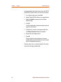
How to use this guide
This guide is designed to make the most of the advantages of
onscreen books. The table of contents, index, and cross
references provide instant links to the information you need.
Just click on the text and jump.
Each chapter about an Advanced Analysis tool is
self-contained. The chapters are organized into these
sections:
■
Overview: introduces you to the tool
■
Strategy: gives you tips on planning your project
■
Procedure: lists each step you need to successfully apply
the tool
■
Example: lists the same steps with an illustrating example
■
For power users: provides background information
If you find printed paper helpful, print only the section you
need at the time. When you want an in-depth tutorial, print the
example. When you want a quick reminder of a procedure,
print the procedure.
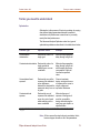
Symbols and conventions
Our documentation uses a few special symbols and
conventions.
Notation
Examples
Description
Bold text
Import Measurements,
Modified LSQ,
PDF Graph
Indicates that text is a menu
or button command, dialog
box option, column or graph
label, or drop-down list option
Icon graphic
10
,
,
Shows the toolbar icon that
should be clicked with your
mouse button to accomplish a
task
PSpice Advanced Analysis Users Guide
Product Version 10.5
Lowercase file
extensions
Related documentation
.aap, .sim, .drt
Indicates a file name
extension
Related documentation
In addition to this guide, you can find technical product
information in the embedded AutoHelp, in related online
documentation, and on our technical website. The table below
describes the type of technical documentation provided with
Advanced Analysis.
This documentation component . . .
Provides this . . .
This guide—
PSpice Advanced Analysis User’s
Guide
A comprehensive guide for understanding and
using the features available in Advanced Analysis.
PSpice Advanced Analysis Users Guide
11
Chapter
Before you begin
Product Version 10.5
This documentation component . . .
Provides this . . .
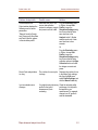
Help system (automatic and manual)
Provides comprehensive information for
understanding the features in Advanced Analysis
and using them to perform specific analyses.
Advanced Analysis provides help in two ways:
automatically (AutoHelp) and manually.
AutoHelp is embedded in its own window and
automatically displays help topics that are
associated with your current activity as you move
about and work within the Advanced Analysis
workspace and interface. It provides immediate
access to information that is relative to your
current task, but lacks the complete set of
navigational tools for accessing other topics.
The manual method lets you open the help system
in a separate browser window and gives you full
navigational access to all topics and resources
outside of the help system.
Using either method, help topics include:
✍
Explanations and instructions for common tasks
✍
Descriptions of menu commands, dialog boxes,
tools on the toolbar and tool palettes, and the
status bar
✍
Glossary terms
✍
Reference information
✍
Product support information
PSpice User’s Guide
An online, searchable user’s guide
PSpice Library List
An online, searchable library list for PSpice model
libraries
PSpice Reference Guide
An online, searchable reference manual for the
PSpice simulation software products
PSpice Quick Reference
Concise descriptions of the commands, shortcuts,
and tools available in PSpice
OrCAD Capture User’s Guide
An online, searchable user’s guide
12
PSpice Advanced Analysis Users Guide
Product Version 10.5
Related documentation
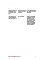
This documentation component . . .
Provides this . . .
OrCAD Capture Quick Reference Card Concise descriptions of the commands, shortcuts,
and tools available in Capture
Accessing online documentation
To access online documentation, you must open the Cadence
Documentation window.
1
Do one of the following:
a.From the Windows Start menu, choose OrCAD 10.0
programs folder and then the Online Documentation
shortcut.
b.From the Help menu in PSpice, choose Manuals.
2
Do one of the following:
a. From the Windows Start menu, choose Cadence
Allegro 15.2 programs folder and then the Online
Documentation shortcut.
b.From the Help menu in AMS Simulator, choose Manuals.
The Cadence Documentation window appears.
3
Click the PSpice category to show the documents in the
category.
4
Double-click a document title to load that document into
your web browser.
PSpice Advanced Analysis Users Guide
13
Chapter
14
Before you begin
Product Version 10.5
PSpice Advanced Analysis Users Guide
Introduction
1
In this chapter
■
Advanced Analysis overview on page 15
■
Project setup on page 16
■
Advanced Analysis files on page 18
■
Workflow on page 18
■
Numerical conventions on page 20
Advanced Analysis overview
Advanced Analysis is an add-on program for PSpice and
PSpice A/D. Use these four Advanced Analysis tools to
improve circuit performance, reliability, and yield:
■
Sensitivity identifies which components have parameters
critical to the measurement goals of your circuit design.
■
The four Optimizer engines optimize the parameters of
key circuit components to meet your performance goals.
■
Smoke warns of component stress due to power
dissipation, increase in junction temperature, secondary
breakdowns, or violations of voltage / current limits.
PSpice Advanced Analysis Users Guide
15
Chapter 1
Introduction
Product Version 10.5
■
Monte Carlo estimates statistical circuit behavior and
yield.
Project setup
Before you begin an Advanced Analysis project, you need:
■
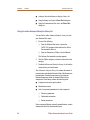
Circuit components that are Advanced Analysis-ready
Only those components that you want tested in Advanced
Analysis have to be Advanced Analysis-ready. See
Chapter 2, “Libraries.”
Note: You can adapt passive RLC components for
Advanced Analysis without choosing them from
parameterized libraries. See Chapter 2, “Libraries.”
■
A circuit drawn in Capture and successfully simulated in
PSpice.
■
PSpice measurements that check circuit behavior critical
to your design.
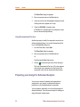
Creating measurement expressions
Sensitivity, Optimizer, and Monte Carlo require measurement
expressions as input. You should create these measurements
expressions in PSpice so you can test the results.
You can also create measurement expressions in Sensitivity,
Optimizer, or Monte Carlo which can be exported to each
other, but these measurements cannot be exported to PSpice
for testing.
16
PSpice Advanced Analysis Users Guide
Product Version 10.5
Project setup
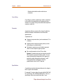
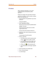
Validating the initial project
Before you use Advanced Analysis:
1
Make your circuit components Advanced-Analysis ready
for the components you want to analyze.
See Chapter 2, “Libraries” for more information.
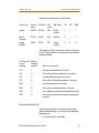
2
Set up a PSpice simulation.
The Advanced Analysis tools use the following
simulations:
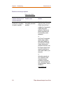
This tool...
Works on these PSpice simulations...
Sensitivity
Time Domain (transient)
DC Sweep
AC Sweep/Noise
Optimizer
Time Domain (transient)
DC Sweep
AC Sweep/Noise
Smoke
Time Domain (transient)
Monte Carlo
Time Domain (transient)
DC Sweep
AC Sweep/Noise
3
Simulate the circuit and make sure the results and
waveforms are what you expect.
4
Define measurements in PSpice to check the circuit
behaviors that are critical for your design. Make sure the
measurement results are what you expect.
Note: For information on setting up circuits, see your
schematic editor user guide, Project setup on page 16,
and Chapter 2, “Libraries.”
For information on setting up simulations, see your
PSpice User’s Guide.
PSpice Advanced Analysis Users Guide
17
Chapter 1
Introduction
Product Version 10.5
For information on setting up measurements, see
“Procedure for creating measurement expressions” on
page 240.
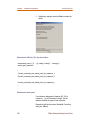
Advanced Analysis files
The principal files used by Advanced Analysis are:
■
PSpice simulation profiles (.sim)
■
Advanced Analysis profiles (.aap)
Advanced users may also use these files:
■
Device property files (.prp)
For more information, see Appendix A, Property Files.
■
Custom derating files for Smoke (.drt)
For more information, see the technical note titled
Creating Custom Derating Files for Advanced
Analysis Smoke on www.orcadpcb.com.
■
Discrete value tables for Optimizer (.table)
For more information, see “What are Discrete Tables?” on
page 131.
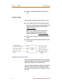
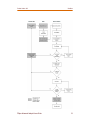
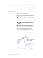
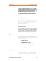
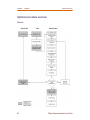
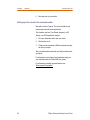
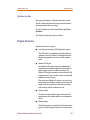
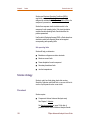
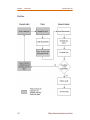
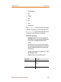
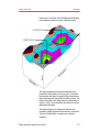
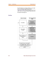
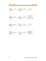
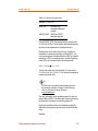
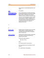
Workflow
There are many ways to use Advanced Analysis. This
workflow shows one way to use all four features.
18
PSpice Advanced Analysis Users Guide
Product Version 10.5
PSpice Advanced Analysis Users Guide
Workflow
19
Chapter 1
Introduction
Product Version 10.5
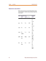
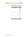
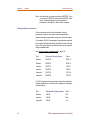
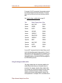
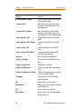
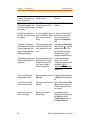
Numerical conventions
PSpice ignores units such as Hz, dB, Farads, Ohms, Henrys,
volts, and amperes. It adds the units automatically, depending
on the context.
Name
Numerical User
value
types in: Or:
Example
Uses
femto-
10-15
2f
F, f
1e-15
2F
2e-15
pico-
10-12
P, p
1e-12
40p
40P
40e-12
nano-
10-9
N, n
1e-9
70n
70N
70e-9
micro-
10-6
U, u
1e-6
.000001
20u
20U
20e-6
milli-
10 -3
M, m
1e-3
.001
30m
30M
30e-3
.03
kilo-
103
1000
K, k
1e+3
2k
2K
2e3
2e+3
2000
20
PSpice Advanced Analysis Users Guide
Product Version 10.5
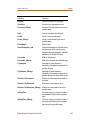
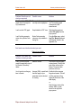
Numerical conventions
Name
Numerical User
value
types in: Or:
mega- 10 6
1,000,000
MEG,
meg
1e+6
Example
Uses
20meg
20MEG
20e6
20e+6
20000000
giga-
109
G, g
1e+9
25g
25G
25e9
25e+9
tera-
1012
T, t
1e+12
30t
30T
30e12
30e+12
PSpice Advanced Analysis Users Guide
21
Chapter 1
22
Introduction
Product Version 10.5
PSpice Advanced Analysis Users Guide
Libraries
2
In this chapter
■
Overview on page 23
■
Using Advanced Analysis libraries on page 27
■
Preparing your design for Advanced Analysis on page 30
■
Example on page 36
■
For power users on page 39
Overview
PSpice ships with over 30 Advanced Analysis libraries
containing over 4,300 components. Separate library lists are
provided for Advanced Analysis libraries and standard PSpice
libraries. The components in the Advanced Analysis libraries
are listed in the Advanced Analysis library list. See Using
the online Advanced Analysis library list on page 28 for
details.
The Advanced Analysis libraries contain parameterized and
standard components. The majority of the components are
parameterized. Standard components in the Advanced
Analysis libraries are similar to components in the standard
PSpice libraries and will not be discussed further in this
document.
PSpice Advanced Analysis Users Guide
23
Chapter 2
Libraries
Product Version 10.5
Parameterized components
A parameter is a physical characteristic of a component that
controls behavior for the component model. In Capture, a
parameter is called a property. A parameter value is either a
number or a variable. When the parameter value is a variable,
you have the option to vary its numerical solution within a
mathematical expression and use it in optimization.
Design EntryWhen the parameter value is a variable, you have
the option to vary its numerical solution within a mathematical
expression and use it in optimization.In the Advanced
Analysis libraries, components may contain one or more of the
following parameters:
■
Tolerance parameters
For example, for a resistor the positive tolerance could be
POSTOL = 10%.
■
Distribution parameters
For example, for a resistor the distribution function used
in Monte Carlo analysis could be DIST = FLAT.
■
Optimizable parameters
For example, for an opamp the gain bandwidth could be
GBW = 10 MHz.
■
Smoke parameters
For example, for a resistor the power maximum operating
condition could be POWER = 0.25 W.
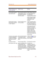
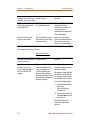
To analyze a circuit component with an Advanced Analysis
tool, make sure the component contains the following
parameters:
24
This Advanced
Analysis tool...
Uses these component
parameters...
Sensitivity
Tolerance parameters
Optimizer
Optimizable parameters
Smoke
Smoke parameters
PSpice Advanced Analysis Users Guide
Product Version 10.5
Overview
This Advanced
Analysis tool...
Uses these component
parameters...
Monte Carlo
Tolerance parameters,
Distribution parameters
(default parameter value is Flat /
Uniform)
Tolerance parameters
Tolerance parameters define the positive and negative
deviation from a component’s nominal value. In order to
include a circuit component in a Sensitivity or Monte Carlo
analysis, the component must have tolerances for the
parameters specified. Use the Advanced Analysis library
list to identify components with parameter tolerances.
In Advanced Analysis, tolerance information includes:
■
Positive tolerance
For example, POSTOL for RLC is the amount a value can
vary in the plus direction.
■
Negative tolerance
For example, NEGTOL for RLC is the amount a value can
vary in the negative direction.
Tolerance values can be entered as percents or absolute
numbers.
Distribution parameters
Distribution parameters define types of distribution functions.
Monte Carlo uses these distribution functions to randomly
select tolerance values within a range.
PSpice Advanced Analysis Users Guide
25
Chapter 2
Libraries
Product Version 10.5
For example, in Capture’s property editor, a resistor could
provide the following information:
Property Value
DIST
FLAT
Optimizable parameters
Optimizable parameters are any characteristics of a model
that you can vary during simulations. In order to include a
circuit component in an Optimizer analysis, the component
must have optimizable parameters. Use the Advanced
Analysis library list to identify components with optimizable
parameters.
For example, in Capture’s property editor, an opamp could
provide the following gain bandwidth:
Property
Value
GBW
1e7
Note that the parameter is available for optimization only if you
add it as a property on the schematic instance and assign it a
value.
During Optimization, the GBW can be varied between any
user-defined limits to achieve the desired specification.
Smoke parameters
Smoke parameters are maximum operating conditions for the
component. To perform a Smoke analysis on a component,
define the smoke parameters for that component. You can still
use non-smoke-defined components in your design, but the
smoke test ignores these components. Use the online
Advanced Analysis library list to identify components with
smoke parameters.
26
PSpice Advanced Analysis Users Guide
Product Version 10.5
Using Advanced Analysis libraries
Most of the analog components in the standard PSpice
libraries also contain smoke parameters. Use the online
PSpice library list to identify components in the standard
PSpice libraries that have smoke parameters.
See also Smoke parameters on page 154.
For example, in Capture’s property editor, a resistor could
provide the following smoke parameter information:
Property
Value
POWER
RMAX
MAX_TEM
P
RTMAX
Use the design variables table to set the values of RMAX and
RTMAX to 0.25 Watts and 200 degrees Centigrade,
respectively.
See Using the design variables table on page 33.
Location of Advanced Analysis libraries
The program installs the Advanced Analysis libraries to the
following locations:
Capture symbol libraries
<Target_directory>\Capture\Library\PSpice\AdvAnls\
PSpice Advanced Analysis model libraries
<Target_directory> \ PSpice \ Library
Using Advanced Analysis libraries
In Capture, there are three ways to quickly identify if a
component is from an Advanced Analysis library:
PSpice Advanced Analysis Users Guide
27
Chapter 2
Libraries
Product Version 10.5
■
Looking in the online Advanced Analysis library list
■
Using the library tool tip in the Place Part dialog box
■
Using the Parameterized Part icon in the Place Part
dialog box
Using the online Advanced Analysis library list
You can find the online Advanced Analysis library list from
your Windows Start menu.
1
Do one of the following:
❑
From the Windows Start menu, choose the
OrCAD 10.0 programs folder and then the Online
Documentation shortcut.
❑
From the Help menu in PSpice, choose Manuals.
The Cadence Documentation window appears.
2
Click the PSpice category to show the documents in the
category.
3
Double-click Advanced Analysis library list to load the
document into your web browser.
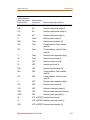
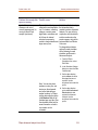
The Advanced Analysis library list contains the names of
parameterized and standard libraries. Most of the libraries are
parameterized. Standard components in the Advanced
Analysis libraries are similar to standard PSpice library
components. Each library contains the following items:
■
Component names and part numbers
■
Manufacturer names
■
Lists of component parameters for each component
❑
Tolerance parameters
❑
Optimizable parameters
❑
Smoke parameters
Some component libraries, primarily opamp libraries, contain
components with all of the parameter types.
28
PSpice Advanced Analysis Users Guide
Product Version 10.5
Using Advanced Analysis libraries
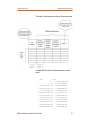
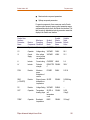
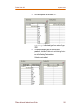
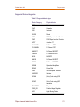
Examples from the library list are shown below:
Device Type
Generic
Name
Part Name
Part
Mfg. Name
Library
TOL
OPT
SMK
Opamp
AD101A
AD101A
OPA
Analog
Devices
Y
Y
Y
Bipolar
Transistor
2N1613
2N1613
BJN
Motorola
N
Y
Y
Analog
Multiplier
AD539
AD539
DRI
Analog
Devices
N
N
N
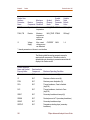
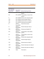
The parameter columns are the three columns on the right in
the list. The abbreviations in the parameter columns have the
following meanings:
This library list With the
column
following
heading...
notation...
Means the component...
TOL
Y
Has tolerance parameters in the model
TOL
N
Does not have tolerance parameters in the model
OPT
Y
Has optimizable parameters in the model
OPT
N
Does not have optimizable parameters in the model
SMK
Y
Has smoke parameters in the model
SMK
N
Does not have smoke parameters in the model
DIST
Y
Has a distribution parameter associated with the model
DIST
N
Does not have a distribution parameter associated with
the model
Using the library tool tip
One easy way to identify if a component comes from an
Advanced Analysis library is to use the tool tip in the Place
Part dialog box.
1
From the Place menu, select Part.
PSpice Advanced Analysis Users Guide
29
Chapter 2
Libraries
Product Version 10.5
The Place Part dialog box appears.
2
Enter a component name in the Part text box.
3
Hover your mouse over the highlighted component name.
A library path name appears in a tool tip.
4
Check for ADVANLS in the path name.
If ADVANLS is in the path name, the component comes
from an Advanced Analysis library.
Using Parameterized Part icon
Another easy way to identify if a component comes from an
Advanced Analysis library is to use the Parameterized Part
icon in the Place Part dialog box.
1
From the Place menu, select Part.
The Place Part dialog box appears.
2
Enter a component name in the Part text box.
Or:
Scroll through the Part List text box
3
Look for
in the lower right corner of the dialog box.
This is the Parameterized Part icon. If this icon appears
when the part name appears in the Part text box, the
component comes from an Advanced Analysis library.
Preparing your design for Advanced Analysis
You may use a mixture of standard and parameterized
components in your design, but Advanced Analysis is
performed on only the parameterized components.
You may create a new design or use an existing design for
Advanced Analysis. There are several steps for making your
design Advanced Analysis-ready.
30
PSpice Advanced Analysis Users Guide
Product Version 10.5
Preparing your design for Advanced Analysis
See “Modifying existing designs for Advanced Analysis” on
page 35.
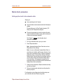
Creating new Advanced Analysis-ready designs
Select parameterized components from Advanced Analysis
libraries.
1
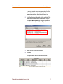
Open the online Advanced Analysis library list found
in Cadence Online Documentation.
2
Find a component marked with a Y in the TOL, OPT, or
SMK columns of the Advanced Analysis library list.
Components marked in this manner are parameterized
components.
3
For that component, write down the Part Library and
Part Name from the Advanced Analysis library list.
4
Add the library to your design in your schematic editor.
5
Place the parameterized component on your schematic.
For example, select the resistor component from the
pspice_elem Advanced Analysis library.
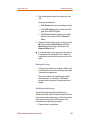
Setting a parameter value
For each parameterized component in your design, set the
parameter value individually on the component using your
schematic editor.
A convenient way to add parameter values on a global basis
is to use the design variable table.
See Using the design variables table on page 33.
Note: If you set a value for POSTOL and leave the value for
NEGTOL blank, Advanced Analysis will automatically
set the value of NEGTOL equal to the value of POSTOL
and perform the analysis.
PSpice Advanced Analysis Users Guide
31
Chapter 2
Libraries
Product Version 10.5
Note: As a minimum, you must set a value for POSTOL. If you
set a value for NEGTOL and leave the POSTOL value
blank, Advanced Analysis will not include the
parameter in Sensitivity or Monte Carlo analyses.
Adding additional parameters
If the component does not have Advanced Analysis
parameters visible on the symbol, add the appropriate
Advanced Analysis parameters using your schematic editor.
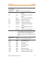
For example: For RLC components, the parameters required
for Advanced Analysis Sensitivity and Monte Carlo are listed
below. The values shown are those that can be set using the
design variables table.
See Using the design variables table on page 33.
Part
Tolerance Property Name
Value
Resistor
POSTOL
RTOL%
Resistor
NEGTOL
RTOL%
Inductor
POSTOL
LTOL%
Inductor
NEGTOL
LTOL%
Capacitor
POSTOL
CTOL%
Capacitor
NEGTOL
CTOL%
For RLC components, the parameter required for Advanced
Analysis Optimizer is the value for the component. Examples
are listed below:
32
Part
Optimizable Property Name
Value
Resistor
VALUE
10K
Inductor
VALUE
33m
Capacitor
VALUE
0.1u
PSpice Advanced Analysis Users Guide
Product Version 10.5
Preparing your design for Advanced Analysis
For example: For RLC components, the parameters required
for Advanced Analysis Smoke are listed below. The values
shown are those that can be set using the design variables
table.
See Using the design variables table on page 33.
Part
Smoke Property Name Value
Resistor
MAX_TEMP
RTMAX
Resistor
POWER
RMAX
Resistor
SLOPE
RSMAX
Resistor
VOLTAGE
RVMAX
Inductor
CURRENT
DIMAX
Inductor
DIELECTRIC
DSMAX
Capacitor
CURRENT
CIMAX
Capacitor
KNEE
CBMAX
Capacitor
MAX_TEMP
CTMAX
Capacitor
SLOPE
CSMAX
Capacitor
VOLTAGE
CMAX
If you use RLC components from the “analog” library, you will
need to add parameters and set values; however, instead of
setting values for the POSTOL and NEGTOL parameters, you
set the values for the TOLERANCE parameter. The positive
and negative tolerance values will use the value assigned to
the TOLERANCE parameter.
Using the design variables table
The design variables table is a component available in the
installed libraries that allows you to set global values for
parameters. For example, using the design variables table,
you can easily set a 5% positive tolerance on all your circuit
resistors. The default information available in the design
variables table includes variable names for tolerance and
smoke parameters. For example, RTOL is a variable name in
PSpice Advanced Analysis Users Guide
33
Chapter 2
Libraries
Product Version 10.5
the design variables tables, which can be used to set POSTOL
(and NEGTOL) tolerance values on all your circuit resistors.
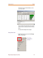
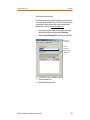
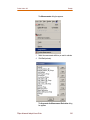
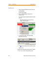
1
From Capture’s Place menu, select Part.
2
Add the PSpice SPECIAL library to your design libraries.
3
Select the Variables component from the PSpice
SPECIAL library.
4
Click OK.
A design variable table of parameter variable names will
appear on the schematic.
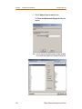
5
Double click on a number in the design variable table.
The Display Properties dialog box will appear.
6
Edit the value in the Value text box.
7
Click OK.
The new numerical value will appear on the design
variables table on the schematic and be used as a global
value for all applicable components.
Parameter values set on a component instance will override
values set in the design variables table.
34
PSpice Advanced Analysis Users Guide
Product Version 10.5
Modifying existing designs for Advanced Analysis
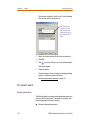
Modifying existing designs for Advanced Analysis
Existing designs that you construct with standard components
will work in Advanced Analysis; however, you can only perform
Advanced Analysis on the parameterized components. To
make sure specific components are Advanced Analysis-ready
(parameterized), do the following steps:
■
Set tolerances for the RLC components
Note: For standard RLC components, the TOLERANCE
property can be used to set tolerance values required for
Sensitivity and Monte Carlo. Standard RLC components
can also be used in the Optimizer.
■
Replace active components with parameterized
components from the Advanced Analysis libraries
■
Add smoke parameters and values to RLC components
PSpice Advanced Analysis Users Guide
35
Chapter 2
Libraries
Product Version 10.5
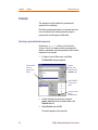
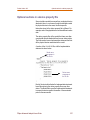
Example
This example is a simple addition of a parameterized
component to a new design.
We’ll add a parameterized resistor to a schematic and show
how to set values for the resistor parameters using the
property editor and the design variables table.
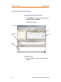
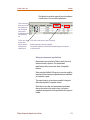
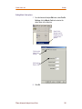
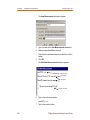
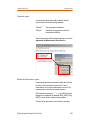
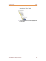
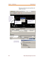
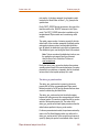
Selecting a parameterized component
We know the pspice_elem library on the Advanced
Analysis library list contains a resistor component with
tolerance, optimizable, and smoke parameters. We’ll use that
component in our example.
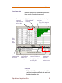
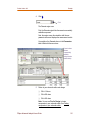
1
In Capture, from the Place menu, select Part.
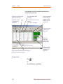
The Place Part dialog box appears.
Add the
pspice_elem
library from the
advanls folder
Select resistor
from the
pspice_elem
library
Note ADVANLS
in library path
name
Icon tells you the
part is
parameterized
2
Use the Add Library browse button to add the
pspice_elem library from the advanls folder to the
Libraries text box.
3
Select Resistor and click OK.
The resistor appears on the schematic.
36
PSpice Advanced Analysis Users Guide
Product Version 10.5
Example
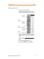
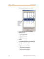
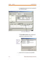
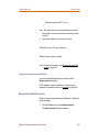
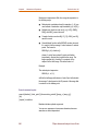
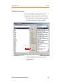
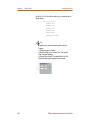
Setting a parameter value
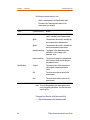
1
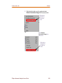
Double click on the Resistor symbol.
The Property Editor appears. Note the Advanced
Analysis parameters already listed for this component.
Distribution
parameter
Smoke
parameter
Tolerance
parameters
Smoke
parameters
Optimizable
parameter
Smoke
parameter
2
Verify that all the parameters required for Sensitivity,
Optimizer, Smoke, and Monte Carlo are visible on the
symbol.
Refer to the tables in Adding additional parameters on
page 32.
3
Set the resistor VALUE parameter to 10k.
4
Set the resistor POSTOL parameter to RTOL%.
PSpice Advanced Analysis Users Guide
37
Chapter 2
Libraries
Product Version 10.5
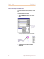
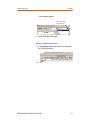
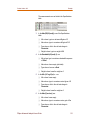
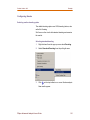
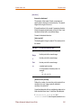
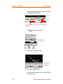
Using the design variables table
Set the resistor parameter values using the design variables
table.
We’ll do one parameter for this resistor.
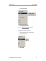
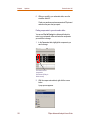
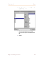
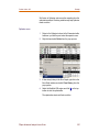
1
Select the Variables part from the PSpice SPECIAL
library.
Note tool tip
with the library
path name
The design variables table appears on the schematic.
Double click on
variable name to edit
value
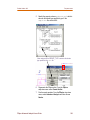
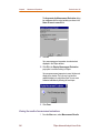
2
38
Double click on the RTOL number 0 in the design
variables table.
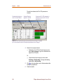
PSpice Advanced Analysis Users Guide
Product Version 10.5
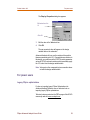
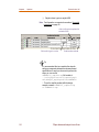
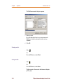
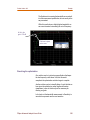
For power users
The Display Properties dialog box appears.
Edit value from 0 to
10
Click OK
3
Edit the value in the Value text box.
4
Click OK.
The new numerical value will appear on the design
variable table on the schematic.
Advanced Analysis will now use the resistor with a positive
tolerance parameter set to 10%. If we added more resistors to
this design, we could then set the POSTOL resistor parameter
values to RTOL% and each resistor would immediately apply
the 10% value from the design variables table.
Note: Values set on the component instance override values
set with the design variables table.
For power users
Legacy PSpice optimizations
For tips on importing legacy PSpice Optimizations into
Advanced Analysis Optimizer, see our technical note on
importing legacy PSpice optimizations.
Technical notes are posted on the PSPice page of the OrCAD
community web site, www.orcadpcb.com.
PSpice Advanced Analysis Users Guide
39
Chapter 2
40
Libraries
Product Version 10.5
PSpice Advanced Analysis Users Guide
Sensitivity
3
In this chapter
■
Sensitivity overview on page 41
■
Sensitivity strategy on page 43
■
Sensitivity procedure on page 44
■
Example on page 53
■
For power users on page 66
Sensitivity overview
Note: Sensitivity analysis is available with the following
products:
❍
PSpice Advanced Optimizer Option
❍
PSpice Advanced Analysis
Sensitivity identifies which components have parameters
critical to the measurement goals of your circuit design.
The Sensitivity Analysis tool examines how much each
component affects circuit behavior by itself and in comparison
to the other components. It also varies all tolerances to create
worst-case (minimum and maximum) measurement values.
PSpice Advanced Analysis Users Guide
41
Chapter 3
Sensitivity
Product Version 10.5
You can use Sensitivity to identify the sensitive components,
then export the components to Optimizer to fine-tune the
circuit behavior.
You can also use Sensitivity to identify which components
affect yield the most, then tighten tolerances of sensitive
components and loosen tolerances of non-sensitive
components. With this information you can evaluate yield
versus cost trade-offs.
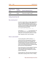
Absolute and relative sensitivity
Sensitivity displays the absolute sensitivity or the relative
sensitivity of a component. Absolute sensitivity is the ratio of
change in a measurement value to a one unit positive change
in the parameter value.
For example: There may be a 0.1V change in voltage for a 1
Ohm change in resistance.
Relative sensitivity is the percentage of change in a
measurement based on a one percent positive change of a
component parameter value.
For example: For each 1 percent change in resistance, there
may be 2 percent change in voltage.
Since capacitor and conductor values are much smaller than
one unit of measurement (Farads or Henries), relative
sensitivity is the more useful calculation.
For more on how this tool calculates sensitivity, see Sensitivity
calculations on page 66.
Absolute sensitivity should be used when the tolerance limits
are not tight or have wide enough bandwidth. Where as
relative sensitivity should be used when the tolerance limits
are tight enough or have less bandwidth. The tolerance
variations are assumed to be linear in this case.
42
PSpice Advanced Analysis Users Guide
Product Version 10.5
Sensitivity strategy
Sensitivity strategy
If Sensitivity analysis shows that the circuit is highly sensitive
to a single parameter, adjust component tolerances on the
schematic and rerun the analysis before continuing on to
Optimizer.
Optimizer works best when all measurements are initially
close to their specification values and require only fine
adjustments.
Plan ahead
Sensitivity requires:
■
Circuit components that are Advanced Analysis-ready
See Chapter 2, Libraries for more information.
■
A circuit design, that is working and can be simulated in
PSpice
■
Measurements set up in PSpice
See Procedure for creating measurement expressions on
page 240
Any circuit components you want to include in the Sensitivity
data need to be Advanced Analysis-ready, with their
tolerances specified.
See Chapter 2, Libraries for more information.
PSpice Advanced Analysis Users Guide
43
Chapter 3
Sensitivity
Product Version 10.5
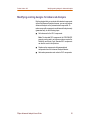
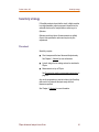
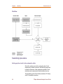
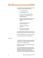
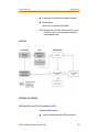
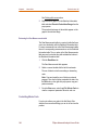
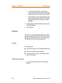
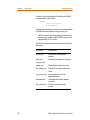
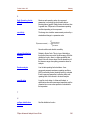
Workflow
Sensitivity procedure
Setting up the circuit in the schematic editor
Start with a working circuit in the schematic editor. Circuit
components you want to include in the Sensitivity data need
to have the tolerances of their parameters specified. Circuit
simulations and measurements should already be set up.
The simulations can be Time Domain (transient), DC Sweep,
and AC Sweep/Noise analyses.
44
PSpice Advanced Analysis Users Guide
Product Version 10.5
Sensitivity procedure
1
Open your circuit from your schematic editor.
2
Run a PSpice simulation.
3
Check your key waveforms in PSpice and make sure they
are what you expect.
4
Check your measurements and make sure they have the
results you expect.
Note: For information on circuit layout and simulation setup,
see your schematic editor and PSpice user guides.
For information on components and the tolerances of their
parameters, see Preparing your design for Advanced Analysis
on page 30.
For information on setting up measurements, see Procedure
for creating measurement expressions on page 240.
For information on testing measurements, see Viewing the
results of measurement evaluations on page 242.
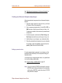
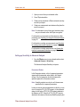
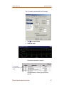
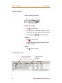
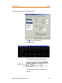
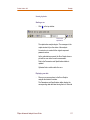
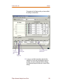
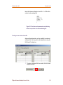
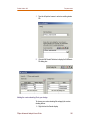
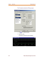
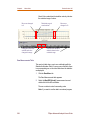
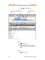
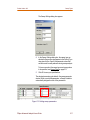
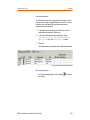
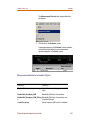
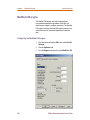
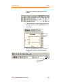
Setting up Sensitivity in Advanced Analysis
1
From the PSpice menu in your schematic editor, select
Advanced Analysis / Sensitivity.
The Advanced Analysis Sensitivity tool opens.
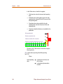
Parameters Window
In the Parameters window, a list of component parameters
appears with the parameter values listed in the Original
column. Only the parameters for which tolerances are
specified appear in the Parameters window.
Note: Sensitivity analysis can only be run if tolerances are
specified for the component parameters.
In case you want to remove a parameter from the list, you can
do so by using the TOL_ON_OFF property. In the schematic
design, set the value of TOL_ON_OFF property attached to
the instance as OFF. If there is no TOL_ON_OFF property
attached to the instance of the device, attach the property and
PSpice Advanced Analysis Users Guide
45
Chapter 3
Sensitivity
Product Version 10.5
set its value to OFF. This is so, because if the tolerance value
is specified for a parameter and TOL_ON_OFF property is not
attached to the component, by default Advanced Analysis
assumes that the value of TOL_ON_OFF property is set to
ON.
In case of hierarchical designs, the value of the TOL_ON_OFF
property attached to the hierarchical block has a higher
priority over the property value attached to the individual
components. For example, if the hierarchical block has the
TOL_ON_OFF property value set to OFF, tolerance values of
all the components within that hierarchical design will be
ignored.
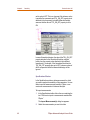
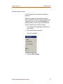
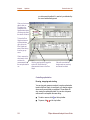
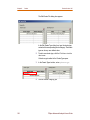
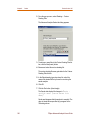
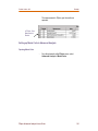
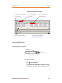
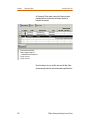
Specifications Window
In the Specifications window, add measurements for which
you want to analyze the sensitivity of the parameters. You can
either import the measurements created in PSpice or can
create new measurements in Advanced Analysis.
To import measurements:
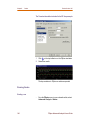
1
In the Specifications table, click on the row containing the
text “Click here to import a measurement created within
PSpice.”
The Import Measurement(s) dialog box appears.
2
46
Select the measurements you want to include.
PSpice Advanced Analysis Users Guide
Product Version 10.5
Sensitivity procedure
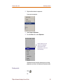
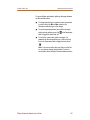
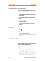
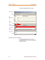
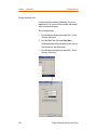
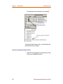
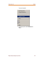
To create new measurements:
1
From the Analysis drop-down menu, choose
Sensitivity / Create New Measurements.
The New Measurement dialog box appears.
2
Create the measurement expression to be evaluated and
click OK.
■
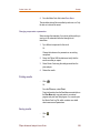
Click
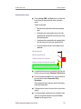
Running Sensitivity
on the top toolbar.
The Sensitivity analysis begins. The messages in the
output window tell you the status of the analysis.
For more information, see Sensitivity calculations on
page 66.
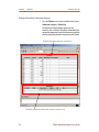
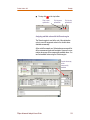
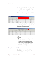
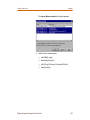
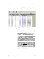
Displaying run data
Sensitivity displays results in two tables for each selected
measurement:
■
■
Parameters table
❑
Parameter values at minimum and maximum
measurement values
❑
Absolute / Relative sensitivities per parameter
❑
Linear / Log bar graphs per parameter
Specifications table
❑
Worst-case min and max measurement values
Sorting data
−
Double click on column headers to sort data in ascending
or descending order.
PSpice Advanced Analysis Users Guide
47
Chapter 3
Sensitivity
Product Version 10.5
Reviewing measurement data
−
Select a measurement on the Specifications table.
A black arrow appears in the left column on the
Specifications table, the row is highlighted, and the Min
and Max columns display the worst-case minimum and
maximum measurement values.
The Parameters table will display the values for
parameters and measurements using the selected
measurement only.
Interpreting @min and @max
Values displayed in the @min and @max columns are the
parameter values at the measurement’s worst-case minimum
and maximum values.
If a measurement value is insensitive to a component, the
sensitivity displayed for that component will be zero. In such
cases, values displayed in the @Min and @Max columns will
be same and will be equal to the Original value of the
component.
Negative and positive sensitivity
If the absolute or the relative sensitivity is negative it implies
that for one unit positive increase in the parameter value, the
measurement value increases in the negative direction.
For example, if for a unit increase in the parameter value, the
measurement value decreases, the component exhibits
negative sensitivity. It can also be that for a unit decrease in
the parameter value, there is an increase in the measurement
value.
On the other hand, positive sensitivity implies that for a unit
increase in the component value, there is an increase in the
measurement value.
48
PSpice Advanced Analysis Users Guide
Product Version 10.5
Sensitivity procedure
Changing from Absolute to Relative sensitivity
1
Right click anywhere in the Parameters table.
2
Select Display / Absolute Sensitivity or Relative
Sensitivity from the pop-up menu.
Note: See Sensitivity calculations on page 66.
Changing bar graph style from linear to log
Most of the sensitivity values can be analyzed using the linear
scale. Logarithmic scale is effective for analyzing the smaller
but non-zero sensitivity values.
To change the bar graph style,
1
Right-click anywhere in the Parameters table.
2
Select Bar Graph Style / Linear or Log from the
pop-up menu.
Important
If 'X' is the bar graph value on a linear scale, then the
bar graph value on the logarithmic scale is not
log (X). The logarithmic values are calculated
separately.
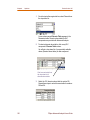
Interpreting <MIN> results
Sensitivity displays <MIN> on the bar graph when sensitivity
values are very small but nonzero.
Interpreting zero results
Sensitivity displays zero in the absolute / relative sensitivity
and bar graph columns if the selected measurement is not
sensitive to the component parameter value.
PSpice Advanced Analysis Users Guide
49
Chapter 3
Sensitivity
Product Version 10.5
Controlling Sensitivity
Data cells with cross-hatched backgrounds are read-only and
cannot be edited. The graphs are also read-only.
Pausing, stopping, and starting
Pausing and resuming
1
Click
on the top toolbar.
The analysis stops, available data is displayed, and the
last completed run number appears in the output window.
2
Click the
or
to resume calculations.
Stopping
−
Click
on the top toolbar.
If a Sensitivity analysis has been stopped, you cannot
resume the analysis.
Sensitivity does not save data from a stopped analysis.
Starting
−
Click
to start or restart.
Controlling measurement specifications
❑
To exclude a measurement specification from
Sensitivity analysis: click
on the applicable
measurement row in the Specifications table.
This removes the check and excludes the
measurement from the next Sensitivity analysis.
❑
To add a new measurement: click on the row
containing the text “Click here to import a
measurement created within PSpice.”
The Import Measurement(s) dialog box appears.
50
PSpice Advanced Analysis Users Guide
Product Version 10.5
Sensitivity procedure
Or:
Right click on the Specifications table and select
Create New Measurement.
The New Measurement dialog box appears.
See Procedure for creating measurement
expressions on page 240.
❑
To export a new measurement to Optimizer or Monte
Carlo, select the measurement and right click on the
row containing the text “Click here to import a
measurement created within PSpice.”
Select Send To from the pop-up menu.
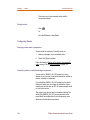
Adjusting component values
Use Find in Design from Advanced Analysis to quickly
return to the schematic editor and change component
information.
For example: You may want to tighten tolerances on
component parameters that are highly sensitive or loosen
tolerances on component parameters that are less sensitive.
1
Right click on the component’s critical parameter in the
Sensitivity Parameters table and select Find in Design
from the pop-up menu.
2
Change the parameter value in the schematic editor.
3
Rerun the simulation and check results.
4
Rerun Sensitivity.
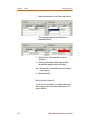
Varying the tolerance range
During Sensitivity analysis, by default Advanced Analysis
varies parameter values by 40% of the tolerance range. You
can modify the default value and specify the percentage by
which the parameter values should be varied within the
tolerance range.
PSpice Advanced Analysis Users Guide
51
Chapter 3
Sensitivity
Product Version 10.5
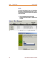
To specify the percentage variation:
1
From the Edit drop-down menu in Advanced Analysis,
choose Profile Settings.
2
In the Profile Settings dialog box, select the Sensitivity
tab.
3
In the Sensitivity Variation text box, specify the
percentage by which you want the parameter values to be
varied.
4
Click OK to save the modifications.
If you now run the Sensitivity analysis, the value specified by
you would be used for calculating the absolute and relative
sensitivity.
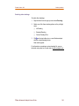
Sending parameters to Optimizer
1
Select the critical parameters in Sensitivity.
2
Right click and select Send to Optimizer from the
pop-up menu.
3
Select Optimizer from the drop-down list on the top
toolbar.
This switches the active window to the Optimizer view
where you can double check that your critical parameters
are listed in the Optimizer Parameters table.
4
Click the Sensitivity tab at the bottom of the Optimizer
Specifications table.
This switches the active window back to the Sensitivity
tool.
Printing results
−
Click
.
Or:
From the File menu, select Print.
52
PSpice Advanced Analysis Users Guide
Product Version 10.5
Sensitivity procedure
Saving results
−
Click
.
Or:
From the File menu, select Save.
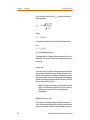
The final results will be saved in the Advanced Analysis
profile (.aap).
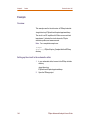
Example
The Advanced Analysis examples folder contains several
demonstration circuits. This example uses the RFAmp circuit.
The circuit contains components with the tolerances of their
parameters specified, so you can use the components without
any modification.
Two PSpice simulation profiles have already been created and
tested. Circuit measurements, entered in PSpice, have been
set up and tested.
Note: See Chapter 2, Libraries for information about setting
tolerances for other circuit examples.
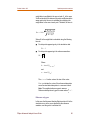
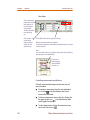
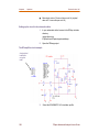
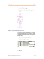
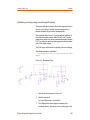
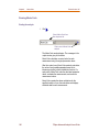
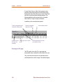
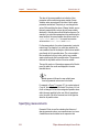
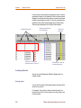
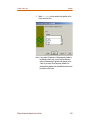
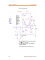
Setting up the circuit in the schematic editor
1
In your schematic editor, browse to the RFAmp tutorials
directory.
<target directory>
\PSpice\tutorial\Capture\pspiceaa\rfamp
PSpice Advanced Analysis Users Guide
53
Chapter 3
Sensitivity
Product Version 10.5
2
Open the RFAmp project.
3
Select the SCHEMATIC1-AC simulation profile.
Assign global
tolerances
using this
table
54
PSpice Advanced Analysis Users Guide
Product Version 10.5
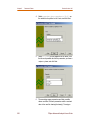
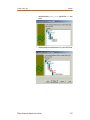
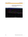
Sensitivity procedure
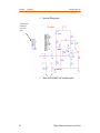
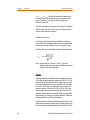
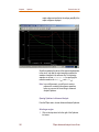
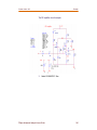
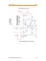
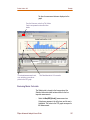
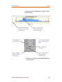
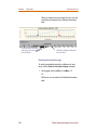
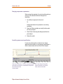
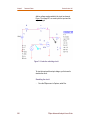
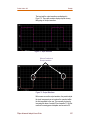
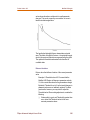
The AC simulation included with the RF example
1
Click
to run the simulation.
2
Review the results.
The waveforms are what we expected.
In the simulator,
view measurement
results
The measurements in PSpice give the results we
expected.
PSpice Advanced Analysis Users Guide
55
Chapter 3
Sensitivity
Product Version 10.5
Setting up Sensitivity in Advanced Analysis
1
From the PSpice menu in your schematic editor, select
Advanced Analysis / Sensitivity.
The Advanced Analysis window opens, and the
Sensitivity tool is activated. Sensitivity automatically lists
component parameters for which tolerances are specified
and the component parameter original (nominal) values.
Sensitivity Parameters table prior to the first run
Sensitivity Specifications table before a project is set up and run
56
PSpice Advanced Analysis Users Guide
Product Version 10.5
Sensitivity procedure
In case you want to remove some parameters from the
Parameters list, you can do so by modifying the
parameter properties in the schematic capture tool.
2
In the Specifications table, right click the row titled, “Click
here to import a measurement created within PSpice.”
The Import Measurement(s) dialog box appears with
measurements configured earlier in PSpice .
3
Select the four ac.sim measurements.
4
Click OK.
The Specifications table lists the measurements.
PSpice Advanced Analysis Users Guide
57
Chapter 3
Sensitivity
Product Version 10.5
Running Sensitivity
−
Click
on the top toolbar.
Click to start
58
PSpice Advanced Analysis Users Guide
Product Version 10.5
Sensitivity procedure
Displaying run data
Results are displayed in the Parameters and Specifications
tables according to the selected measurement.
Parameter values that
correspond to
measurement min
and max values
Right click to change
Display to Absolute
Sensitivity
Double click column headings to cha
the sort order
Right click to change bar
from Linear to Log
Click to
exclude
from
analysis
Click to select the
measurement data
set for review
Hover your mouse
over a red flag to
read the error
messages
Min means that the sensitivity
is very small, but not zero
A zero (0) displays if there is
no sensitivity at all
The
measurement’s
worst-case
minimum and
maximum values
Sorting data
−
Double click on the Linear column header to sort the bar
graph data in ascending order. Double click again to sort
the data in descending order.
PSpice Advanced Analysis Users Guide
59
Chapter 3
Sensitivity
Product Version 10.5
Selecting the measurement to view
−
Select a measurement in the Specifications table.
The data in the Parameters table relates to the
measurement you selected.
Table...
Column heading...
Means...
Parameters
Original
The nominal component parameter values
used to calculate nominal measurement.
@Min
The parameter value used to calculate the
worst-case minimum measurement.
@Max
The parameter value used to calculate the
worst-case maximum measurement.
absolute sensitivity
The change in the measurement value
divided by a unit of change in the
parameter value.
relative sensitivity
The percent of change in a measurement
value based on a one percent change in
the parameter value.
Original
The nominal value of the measurement
using original component parameter
values.
Min
The worst-case minimum value for the
measurement.
Max
The worst-case maximum value for the
measurement.
Specifications
Note: To see all the parameter and measurement values
used in Sensitivity calculations: from the View menu,
select Log File.
Changing from Absolute to Relative sensitivity
1
60
Right click anywhere on the Parameters table.
PSpice Advanced Analysis Users Guide
Product Version 10.5
Sensitivity procedure
A pop-up menu appears
2
Select Relative Sensitivity.
Note: See Sensitivity calculations on page 66.
Changing the bar graph to linear view
1
Right click anywhere on the Parameters table.
A pop-up menu appears.
2
Select Linear.
PSpice Advanced Analysis Users Guide
61
Chapter 3
Sensitivity
Product Version 10.5
Controlling Sensitivity
Pausing, stopping, and starting
Click to stop
Click to start
Click to pause
Pausing and resuming
1
Click
on the top toolbar.
The analysis stops, available data is displayed, and the
last completed run number appears in the output window.
2
Click the depressed
or
to resume calculations.
Stopping
−
Click
on the top toolbar.
If a Sensitivity analysis has been stopped, you cannot
resume the analysis.
Starting
−
Click
to start or resume.
Controlling Measurements
Click to remove this check
mark and exclude this
measurement from analysis
62
Click here to edit the
measurement
expression
PSpice Advanced Analysis Users Guide
Product Version 10.5
Sensitivity procedure
Adjusting component values
In the RF example, we will not change any component
parameters.
With another example you may decide after reviewing
sensitivity results that you want to change component values
or tighten tolerances. You can use Find in Design from
Advanced Analysis to return to your schematic editor and
locate the components you would like to change.
1
In the Parameters table, highlight the components you
want to change.
2
Right click the selected components.
A pop-up menu appears.
3
Left click on Find in Design.
PSpice Advanced Analysis Users Guide
63
Chapter 3
Sensitivity
Product Version 10.5
The schematic editor appears with the components
highlighted.
4
Change the parameter value in the schematic editor.
5
Rerun the PSpice simulation and check results.
6
Rerun Sensitivity.
Sending parameters to Optimizer
Review the results of the Sensitivity calculations. We need to
use engineering judgment to select the sensitive components
to optimize:
■
We won’t change R5 or R9 because they control the input
and output impedances.
■
We won’t change R2 or R3 because they control
transistor biasing.
The linear bar graph at the Relative Sensitivity setting shows
that R4, R6, and R8 are also critical parameters. We’ll import
these parameters and values to Optimizer.
1
64
In the Parameters table, hold down the Ctrl key and select
R4, R6, and R8.
PSpice Advanced Analysis Users Guide
Product Version 10.5
Sensitivity procedure
2
Right click the selected components.
A pop-up menu appears.
3
Select Send to Optimizer.
4
From the View menu, select Optimizer.
Select Optimizer view to
switch to the Optimizer
window and see the
parameters you sent over
from Sensitivity
Optimizer becomes the active window and your critical
parameters are listed in the Optimizer Parameters table.
Printing results
−
Click
.
Or:
PSpice Advanced Analysis Users Guide
65
Chapter 3
Sensitivity
Product Version 10.5
From the File menu, select Print.
Saving results
−
Click
.
Or:
From the File menu, select Save.
The final results will be saved in the Advanced Analysis
profile (.aap).
For power users
Sensitivity calculations
Absolute sensitivity
Absolute sensitivity is the ratio of change in a measurement
value to a one unit positive change in the parameter value.
For example: There may be a 0.1V change in voltage for a 1
Ohm change in resistance.
The formula for absolute sensitivity is:
[(Ms - Mn) / (Pn * Sv * Tol)]
Where:
M s = the measurement from the sensitivity run for that
parameter
M n = the measurement from the nominal run
Tol = relative tolerance of the parameter
P n = Nominal parameter value
Sv = Sensitivity
Variation. (Default = 40%)
By default, the parameter value is varied within 40% of the set
tolerance.
66
PSpice Advanced Analysis Users Guide
Product Version 10.5
Sensitivity procedure
You can change this value to any desired percentage using
the Profile settings dialog box.
1
From the Edit drop-down menu, choose Profile Settings.
2
In the Profile setting dialog box, select the Sensitivity tab.
3
In the Sensitivity Variation dialog box, specify the value by
which you want to vary the parameter value.
4
Click OK to save your settings.
The values entered by you in the Profile Setting dialog box, are
stored for the future use as well. Every time you load the
project, old values are used for advanced analysis
simulations.
Example
For example, if you specify the Sensitivity Variation as 10%,
the parameter values will be varied within 10% of the tolerance
value.
Consider that you want to test a resistor of 100k for sensitivity.
The tolerance value attached to the resistor is 10%.
By default, for sensitivity calculations, the value of resistor will
be varied from 96K to 104K. But if you change thedefault
value of Sensitiviy Variation to 10%, the resistor values will be
varied from 99K to 101K for sensitivity calculations.
Relative sensitivity
Relative sensitivity is the percentage of change in a
measurement based on a one percent positive change of a
component’s parameter value.
For example: For each 1 percent change in resistance, there
may be 2 percent change in voltage.
The formula for relative sensitivity is:
[(Ms - Mn) / (Sv*Tol)]
Where:
PSpice Advanced Analysis Users Guide
67
Chapter 3
Sensitivity
Product Version 10.5
M s = the measurement from the sensitivity run for that
parameter
M n = the measurement from the nominal run
Tol = relative tolerance of the parameter
Sv = Sensitivity
Variation. (Default = 40%)
Relative sensitivity calculations determine the measurement
change between simulations with the component parameter
first set at its original value and then changed by Sv percent
of its positive tolerance. Linearity is assumed. This approach
reduces numerical calculation errors related to small
differences.
For example, assume that an analysis is run on a 100-ohm
resistor which has a tolerance of 10 percent. The maximum
value for the resistor would be 110 ohms. Assuming the
default value of Sv, which is 40%, the analysis is run with the
value of the resistor set to 104 ohms (40 percent of the 10 ohm
tolerance) and a measurement value is obtained. Using that
value as a base, Sensitivity assumes that the resistance
change from 100 to 104 ohms is linear and calculates
(interpolates) the measured value at 1 percent tolerance (101
ohms).
Worst-case minimums and maximums
For each measurement, Sensitivity sets all parameters to their
tolerance limits in the direction that will increase the
measurement value, runs a simulation, and records the
measurement value. Sensitivity then sets the parameters to
the opposite tolerance limits and gets the resulting value.
If worst-case measurement values are within acceptable limits
for the design, the measurements can in most cases be
ignored for the purpose of optimization.
Sensitivity assumes that the measured quantity varies
monotonically throughout the range of tolerances. If not (if
there is an inflection point in the curve of output function
values), the tool does not detect it. Symptoms of this include
68
PSpice Advanced Analysis Users Guide
Product Version 10.5
Sensitivity procedure
a maximum worst-case value that is less than the original
value, or a minimum value greater than the original value.
Sensitivity analysis runs
Sensitivity performs the following runs:
■
A nominal run with all parameters set at original values
■
The next run with one parameter varied within tolerance
Values are obtained for each measurement. View the Log
File for parameter values used in each measurement
calculation.
■
Subsequent runs with one parameter varied within
tolerance
■
A minimum worst-case run for each measurement
■
A maximum worst-case run for each measurement
For our example circuit with 4 measurements and 12
parameters with tolerances, Sensitivity performs 21 runs.
There is one worst-case
minimum and one
worst-case maximum run per
measurement
1 + 12 + (2 x 4) = 21 runs
The nominal
run using the
original
parameter
values
There are four measurements
used in this example
There is one run for each
parameter varied within tolerance.
We use 12 parameters
To see the details of parameter and measurement
calculations: from the View menu select Log File.
PSpice Advanced Analysis Users Guide
69
Chapter 3
70
Sensitivity
Product Version 10.5
PSpice Advanced Analysis Users Guide
Optimizer
4
In this chapter
This chapter introduces you to Optimizer, its function, and the
optimization process.
■
Optimizer overview on page 71
■
Terms you need to understand on page 73
■
Optimizer procedure overview on page 80
■
Example on page 107
■
For Power Users on page 131
Optimizer overview
Note: Advanced Analysis Optimizer is available with the
following products:
❍
PSpice Advanced Optimizer Option
❍
PSpice Advanced Analysis
❍
PSpice Optimizer
Optimizer is a design tool for optimizing analog circuits and
their behavior. It helps you modify and optimize analog
designs to meet your performance goals.
PSpice Advanced Analysis Users Guide
71
Chapter 4
Optimizer
Product Version 10.5
Optimizer fine tunes your designs faster and automatically
than trial and error bench testing can. Use Optimizer to find
the best component or system values for your specifications.
Advanced Analysis Optimizer can be used to optimize the
designs that meet the following criteria:
■
Design should simulate with PSpice.
You can optimize a working circuit design that can be
simulated using PSpice and the simulation results are as
desired.
■
Components in the design must have variable
parameters, each of which relates to an intended
performance goal.
Optimizer cannot be used to:
■
Create a working design
■
Optimize a digital design or a design in which the circuit
has several states and small changes in the variable
parameter values causes a change of state. For example,
a flip-flop is on for some parameter value, and off for a
slightly different value.
You can use the Advanced Analysis Optimizer to import
legacy Optimizer projects. For view the detailed procedure,
see the technical note posted on the OrCAD community site,
www.orcadpcb.com. All PSpice related technical notes posted
on the community site are available under Application Notes
section of the PSpice page.
72
PSpice Advanced Analysis Users Guide
Product Version 10.5
Terms you need to understand
Terms you need to understand
Optimization
Optimization is the process of fine-tuning a design by varying
user-defined design parameters between successive
simulations until performance comes close to (or exactly
meets) the ideal performance.
The Advanced Analysis Optimizer solves four types of
optimization problems as described in the table shown below.
Problem Type
Optimizer Action
Example
Unconstrained
minimization
Reduces the value of a
single goal
Minimize the propagation
delay through a logic cell
Constrained minimization Reduces the value of a
single goal while
satisfying one or more
constraints
Minimize the propagation
delay through a logic cell
while keeping the power
consumption of the cell
less than a specified
value
Unconstrained least
squares1
Reduces the sum of the
squares of the individual
errors (difference
between the ideal and the
measured value) for a set
of goals
Given a terminator
design, minimize the sum
of squares of the errors in
output voltage and
equivalent resistance
Constrained least
squares
Reduces the sum of
squares of the individual
errors for a set of goals
while satisfying one or
more constraints
Minimize the sum of
squares of the figures of
merit for an amplifier
design while keeping the
open loop gain equal to a
specified value
1 Use unconstrained least squares when fitting model parameters to a set of measurements, or when minimizing more than
one goal.
Note: All four cases allow simple bound constraints; that is,
lower and upper bounds on all of the parameters.
PSpice Advanced Analysis Users Guide
73
Chapter 4
Optimizer
Product Version 10.5
Optimizer also handles nonlinear function as
constraints.
Curve fitting
Curve fitting is a method of optimizing a model to a waveform.
In this method, the specifications are represented using a
collection of x-y points. These points describe the response of
a system or a part of it.
Parameter
A parameter defines a property of the design for which the
Optimizer attempts to determine the best value within
specified limits.
A parameter can:
■
Represent component values (such as resistance, R, for
a resistor).
■
Represent other component property values (such as
slider settings in a potentiometer).
■
Participate in expressions used to define component
values or other component property values.
■
Be a model parameter, such as IS for a diode.
Example: A potentiometer part in a schematic uses the
SET property to represent the slider position. You can
assign a parameterized expression to this property to
represent variable slider positions between 1 and 0.
During optimization, the Optimizer varies the
parameterized value of the SET property.
Specification
A specification describes the desired behavior of a design in
terms of goals and constraints.
For example: For a given design, the gain shall be 20 dB 1dB;
for a given design, the 3 dB bandwidth shall be 1 kHz; for a
given design, the rise time must be less than 1 usec.
74
PSpice Advanced Analysis Users Guide
Product Version 10.5
Terms you need to understand
A design must always have at least one goal. You can have
any number of goals and constraints in any combination, but it
is recommended that the number of goals should be less. You
can easily change a goal to a constraint and vice-versa.
The Advanced Analysis Optimizer can have two types of
specifications: internal and external.
Internal specifications
An internal specification is composed of goals and constraints
that are defined in terms of target values and ranges. These
specifications are entered using the Standard tab of the
Advanced Analysis Optimizer.
External specifications
An external specification is composed of measurement data
defined in an external data file, which is read by the Advanced
Analysis Optimizer. The external specifications are entered
using the Curve Fit tab of the Advanced Analysis Optimizer.
Goal
A goal defines the performance level that the design should
attempt to meet (for instance, minimum power consumption).
A goal specification includes:
❑
The name of the goal.
❑
An acceptable range of values.
❑
A circuit file to simulate, a simulation profile.
❑
An expression or a measurement function for
measuring performance.
Constraint
A constraint defines the performance level that the design
must fulfill. For example, an expression indicating that the
PSpice Advanced Analysis Users Guide
75
Chapter 4
Optimizer
Product Version 10.5
output voltage that must be greater than a specific level can be
a constraint. The constraint specification includes:
❑
The name of the constraint.
❑
An acceptable range of values.
❑
A circuit file to simulate or a simulation profile.
❑
An expression or a measurement function for
measuring performance.
❑
An allowed relationship between measured values
and the target value, which can be one of the
following:
<=
measured value must be less than
or equal to the target value
=
measured value must equal the
target value
>=
measured value must be greater
than or equal to the target value
It is recommended that in a design, nonlinear functions of the
parameters should be treated as constraints and not as goals.
For example: Bandwidth can vary as the square root of a bias
current and as the reciprocal of a transistor dimension.
Performance
The performance of a design is a measure of how closely the
calculated values of its specifications approach their target
values for a given set of parameter values.
Each aspect of a design’s performance is found by evaluating
Optimizer expressionsL
In many cases (particularly if there are multiple conflicting
specifications), it is possible that the Optimizer will not meet all
of the goals and constraints. In these cases, optimum
performance is the best compromise solution—that is, the
solution that comes closest to satisfying each of the goals and
76
PSpice Advanced Analysis Users Guide
Product Version 10.5
Terms you need to understand
constraints, even though it may not completely satisfy any
single one.
Evaluation
An evaluation is an algorithm that computes a single
numerical value, which is used as the measure of
performance with respect to a design specification.
The Optimizer accepts evaluations in one of these three
forms:
■
Single-point PSpice A/DAMS trace function
■
PSpice A/DAMS goal function
■
Expression based on a combination of functions. For
example max(X)+max(Y)
Given evaluation results, the Optimizer determines whether or
not the changes in parameter values are improving
performance, and determines how to select the parameters
for the next iteration.
Trace function
A trace function defines how to evaluate a design
characteristic when running a single-point analysis (such as a
DC sweep with a fixed voltage input of 5 V). For example:
V(out) to measure the output voltage; I(d1) to measure the
current through a component.
Note: Refer to the online PSpice A/D Reference Guide
for the variable formats and mathematical functions you
can use to specify a trace function.
Goal function
A goal function defines how to evaluate a design characteristic
when running any kind of analysis other than a single-point
sweep analysis. A goal function computes a single number
from a waveform. This can be done by finding a characteristic
PSpice Advanced Analysis Users Guide
77
Chapter 4
Optimizer
Product Version 10.5
point (e.g., time of a zero-crossing) or by some other
operation.
For example, you can use a goal functions to:
■
Find maxima and minima in a trace.
■
Find distance between two characteristic points (such as
peaks).
■
Measure slope of a line segment.
■
Derive aspects of the circuit’s performance which are
mathematically described (such as 3 dB bandwidth,
power consumption, and gain and phase margin).
To write effective goal functions, determine what you are
attempting to measure, then define what is mathematically
special about that point (or set of points).
Note: Be sure that the goal functions accurately measure
what they are intended to measure. Optimization
results highly depend on how well the goal functions
behave. Discontinuities in goal functions (i.e., sudden
jumps for small parameter changes) can cause the
optimization process to fail.
Optimizer expression
An expression defines a design characteristic. The expression
is composed of optimizer parameter values, constants, and
the operators and functions shown in Table 4-1.
For example: To measure the sum of resistor values for two
resistors with parameterized values named R1val and R2val,
respectively, use the expression R1val + R2val.
Table 4-1 Valid Operators and Functions for Advanced
Analysis Optimizer Expressions.
78
Operator
Meaning
+
addition
-
subtraction
PSpice Advanced Analysis Users Guide
Product Version 10.5
Terms you need to understand
Table 4-1 Valid Operators and Functions for Advanced
Analysis Optimizer Expressions., continued
Operator
Meaning
*
multiplication
/
division
**
exponentiation
exp
ex
log
ln(x)
log10
log 10 (x)
sin
sine
cos
cosine
tan
tangent
atan
arctangent
Note: Unlike trace functions and goal functions, Optimizer
expressions are evaluated without using a simulation.
Derivative
A derivative can be defined as the rate of change of
specification value with the change in parameter value.
Simulation profile
A simulation profile is used in the basic simulation flow. A
simulation profile contains and saves the simulation settings
for an analysis type so that it can be reused.
Advanced Analysis Profile
An advanced analysis profile contains and saves the
advanced analyses (optimizer/sensitivity) settings so it can be
reused.
PSpice Advanced Analysis Users Guide
79
Chapter 4
Optimizer
Product Version 10.5
Optimizer procedure overview
Workflow
80
PSpice Advanced Analysis Users Guide
Product Version 10.5
Optimizer procedure overview
To obtain meaningful optimization results, the Optimizer
requires a problem description that consists of a circuit design,
a list of optimization parameters, number of problem
constraints derived from the design specification, and a set of
performance goals to optimize.
To optimize a circuit,
1
Create or edit a circuit using Capture.
2
Simulate and define circuit measurements.
3
Determine and set up optimization parameters that you
want to vary during optimization.
You can set up parameters from the Optimizer or on the
schematic.
4
Specify the optimization specification.
■
For Internal specifications use the standard tab.
a. Define the goal for the circuit measurements.
You can define goals such as rise time, phase
margin, or entire response curves.
b. Weight goals as needed.
■
For External specifications use the Curve Fit tab.
a. Specify the trace expression and the location of the
reference file.
b. For each of the Trace expression, specify the
reference waveform, tolerance, and weight.
5
Select the Optimizer engine.
You can use either the Least Squares Quadratic, Modified
Least Squares Quadratic, or Random engines for
optimization. The Discrete engine should be used after
optimization to convert optimization parameters into
discrete values only.
6
Start the analysis from the Optimizer.
7
Analyze or review the data in the Optimizer and refine the
circuit design.
PSpice Advanced Analysis Users Guide
81
Chapter 4
Optimizer
Product Version 10.5
8
Save and print out your results.
Setting up in the circuit in the schematic editor
Start with a circuit in Capture. The circuit simulations and
measurements should be already defined.
The simulation can be a Time Domain (transient), a DC
Sweep, or an AC Sweep/Noise analysis.
1
From your schematic editor, open your circuit.
2
Simulate the circuit.
3
Check your key waveforms in PSpice and make sure they
are what you expect.
Test your measurements and make sure they have the results
you expect.
For information on circuit layout, and simulation setup, see
your schematic editor or PSpice AMS user guides.
For information on setting up measurements, see
“Measurement Expressions."
82
PSpice Advanced Analysis Users Guide
Product Version 10.5
Optimizer procedure overview
Setting up Optimizer in Advanced Analysis
Setting up the Optimizer consists of the following tasks:
■
Opening Optimizer in Advanced Analysis
■
Selecting an engine
■
Defining Optimization parameters (Selecting Component
Parameters)
■
Setting up circuit measurements or specifications.
■
Specifying optimization goals
Optimization goals are design specifications that you want to
meet. Therefore, while defining optimization parameters, you
need to determine parameters that affect your goals the most.
Opening Optimizer in Advanced Analysis
−
From the PSpice menu in your schematic editor, select
Advanced Analysis / Optimizer.
The Advanced Analysis Optimizer tool opens.
Selecting an engine
Optimizer in advanced analysis supports multiple engines.
These are Least Square (LSQ), Modified LSQ (MLSQ),
Random, and Discrete engines. In an optimization cycle, a
combination of these engines is used.
Use these Optimizer engines for these reasons:
■
Modified LSQ engine: to rapidly converge on an optimum
solution.
■
LSQ engine: to converge on an optimum solution if the
Modified LSQ engine did not get close enough.
■
Random engine: to pick a starting point that avoids
getting stuck in local minima when there is a problem
converging.
See Local and global minimums on page 270.
PSpice Advanced Analysis Users Guide
83
Chapter 4
Optimizer
Product Version 10.5
■
Discrete engine: to pick commercially available
component values and run the simulation one more time
with the selected commercial values.
The normal flow in which these engines are used is Random
engine, followed by LSQ or MLSQ engine, and finally the
Discrete engine.
To know more about the Optimizer engines see Engine
overview.
−
From the top toolbar engine drop-down list, select one of
the four optimizing engines.
Note: The Discrete engine is used at the end of the
optimization cycle to round off component values to
commercially available values.
Setting up component parameters
In this step, you identify the components or the parts in the
circuit, whose parameter values you need to vary. Though the
Optimizer in Advanced Analysis can support any number of
components, it is recommended that the number of
components with the variable parameter values should be
kept to minimum.
You can specify parameters using:
■
Schematic Editor
■
Optimizer
■
Sensitivity
Schematic Editor
1
In the schematic editor, select the component, whose
parameter values you want to vary.
2
Select PSpice > Advanced Analysis > Export
Parameters to Optimizer.
The component gets added in the Parameters table.
84
PSpice Advanced Analysis Users Guide
Product Version 10.5
Optimizer procedure overview
Note: After you select the component, you can right-click and
select Export Parameters to Optimizer from the
pop-up menu. This command is enabled only if the
selected component is based on PSpice-provided
templates.
Optimizer
1
In the Parameters table in Advanced Analysis, click on the
row containing the text “Click here to import.”
The Parameters Selection dialog box appears.
2
Highlight the components you want to vary and click OK.
The components are now listed in the Parameters table.
Sensitivity
1
After you run the sensitivity analysis, select the most
sensitive components and right-click.
2
From the pop-up menu, select Send to Optimizer.
Selected components are listed in the Parameters table.
When you add a component to the Parameters table, the
parameter name, the original value of the parameter, and the
minimum and maximum values of the parameter are also
listed in the Parameters table. The Min and Max values sets
the range the engine will vary the component’s parameters.
These values are calculated by the Optimizer based on the
original value. By default, Min value is one-tenth of the
Original value and Max value is ten times the Original
value.
You can use your engineering judgment to edit the Parameters
table Min and Max values for the Optimization.
PSpice Advanced Analysis Users Guide
85
Chapter 4
Optimizer
Product Version 10.5
Caution
If you reimport any of the parameter that is
already present in the Parameters table, the
entries in the Original, Min, and Max columns are
overwritten by the new values.
Guidelines for selecting components
Optimization parameters need to carefully selected to ensure
quicker optimizations and the best results.
■
Vary your specification’s most sensitive components. Run
a sensitivity analysis to find them.
■
Use good engineering judgment. Don’t vary components
whose values need to stay the same for successful circuit
operation.
For example: if the input and output resistors need to be
50 ohms for impedance matching, do not choose those
components to optimize.
■
Vary just one component if varying other components can
cause the same effect.
For example: in an RC filter combination, both the resistor
and capacitor affect the bandwidth. Selecting one
parameter simplifies the problem. If your goal cannot be
met with one parameter, you can add the second
parameter.
Guidelines for setting up Parameters
■
Make sure that ranges you specify take into account
power dissipation and component cost.
For example: a resistor with a small value (low ohms)
could require a larger, more expensive power rating.
■
86
Start with a small set of parameters (three or four) and
add to the list during your optimization process, especially
when running the LSQ engine.
PSpice Advanced Analysis Users Guide
Product Version 10.5
Optimizer procedure overview
■
Aim for parameters with initial values near the range
midpoints. Optimizer has more trouble finding solutions if
parameter values are close to the endpoint of the ranges.
■
Keep optimization parameter ranges within 1 or 2 orders
of magnitude.
Setting up specifications
Using the Advanced Analysis Optimizer you can set two types
of specifications:
■
Measurement specifications - should be used in cases
where circuit performance is measurable in terms of
variable parameter values, such as gain margin for the
circuit.
■
Curve-fit specifications - should be used in cases where
circuit output is a waveform, such as in wave shaping
circuits.
Setting up measurement specifications
In the Advanced Analysis Optimizer, you can specify the
measurement specification in the Standard tab.
1
In the Specifications table, click on the row containing the
text “Click here to import...”
The Import Measurements dialog box appears with
measurements configured earlier in PSpice.
2
Highlight the measurements you want to vary and click
OK.
The components are now listed in the Specifications
table.
3
Specify the acceptable minimum and maximum
measurement values in the Specifications table Min and
Max columns.
4
If you are using the Modified LSQ engine, mark the
measurement as a goal or constraint by clicking in the
Type column.
PSpice Advanced Analysis Users Guide
87
Chapter 4
Optimizer
Product Version 10.5
The engine strives to get as close as possible to the goals
while ensuring that the constraints are met.
5
Weigh the importance of the specification using the
Weight column.
Change the number in the weight column if you want to
emphasize the importance of one specification with
respect to another. Use a positive integer greater than or
equal to one.
Note: Trial and error experimenting is usually the best way to
select an appropriate weight. Pick one weight and
check the Optimizer results on the Error Graph. If the
results do not emphasize the weighted trace more than
the rest of the traces on the graph, pick a higher weight
and rerun the Optimization. Repeat until you get the
desired results.
Guidelines for setting up measurement specifications
■
Determine your requirements first, then how to measure
them.
■
Don’t set conflicting goals.
For example: Vout > 5 and Vout < 2 when the input is 3V.
■
Make sure enough data points are generated around the
points of measurements. Good resolution is required for
consistent and accurate measurements.
■
Simulate only what’s needed to measure your goal.
For example: for a high frequency filter, start your
frequency sweep at 100 kHz instead of 1 Hz.
Setting up curve-fit specifications
Use curve fitting for following:
1
88
To optimize a model to one or more sets of data points.
Using curve fitting, you can optimize multiple model
parameters to match the actual device characteristic
represented either waveforms from data sheets or
measured data.
PSpice Advanced Analysis Users Guide
Product Version 10.5
Optimizer procedure overview
2
When the goal functions are specified as values at
particular points, YatX().
3
To optimize circuits that need a precise AC or impulse
response. For example, you can use curve fitting for
optimizing signal shaping circuits, where the circuit
waveform must match the reference waveform.
To use curve fitting for optimizing a design, you need to specify
the following in the Curve Fit tab of the Advanced Analysis
Optimizer:
1
A curve-fit specification
You can either import a specification from an existing
.opt file or can create a new specification.
Creating a new specification includes specifying a trace
expression, a reference file containing measured points
and the corresponding measurement values, and a
reference waveform.
To know the details about the New Trace Expression
dialog box, see Advanced Analysis Online Help.
To see the detailed procedure for creating a new curve-fit
specification, see “Creating a Curve-fit Specification”
on page 89.
To know more about the reference files, see Reference
file on page 90.
2
List of parameters to be changed
All the optimizable parameters in a circuit are listed in the
property map file. This file is created when you netlist the
design, and has information of each of the device used in
the circuit design.
Creating a Curve-fit Specification
1
Specify the Trace Expression.
a. In the Specifications area, click the row stating “Click
here to enter a curve-fit specification”.
PSpice Advanced Analysis Users Guide
89
Chapter 4
Optimizer
Product Version 10.5
b. In the New Trace Expression dialog box, select the
simulation profile from the Profile drop-down list, and
also specify the trace expression or the
measurement for which you want to optimize the
design.
2
Specify the reference file.
3
Specify the reference waveform. The Ref. Waveform
drop-down list box lists all the reference waveforms
present in the reference file that is specified in the
previous step.
4
Specify the Weight for the specification.
5
Specify the relative tolerance.
Reference file
To be able to use curve fitting for optimizing your circuit, you
must have a reference waveform. In Advanced Analysis
Optimizer, the reference waveform is specified in form of
multiple data points stored in a reference file. A reference file
is a text file that contains the reference waveform with respect
to a sweep in the tabular form with the data values separated
by white spaces, blanks, tabs or comma.
An reference file has to have a minimum of two columns, one
for the sweep data and one for the reference waveform. A
reference file can have multiple columns. Each extra column
represents a different reference waveform.
90
PSpice Advanced Analysis Users Guide
Product Version 10.5
Optimizer procedure overview
The format of a multiple column reference file is shown below:
A sample MDP file with one reference waveform is shown
below.
Time
V(D4:2)
0
1.35092732941686e-022
2e-010
0.119616948068142
2.17331331036985e-010
0.129942461848259
2.51993993110955e-010
0.150499030947685
3.21319317258894e-010
0.19108946621418
4.59969965554774e-010
0.270239174365997
7.37271262146533e-010
0.420916199684143
1.14672723207623e-009
0.627191662788391
1.52335408125073e-009
0.802674531936646
2.27660777959973e-009
1.13146245479584
3.77361568603665e-009
1.87895023822784
6.76763149891049e-009
3.6644229888916
PSpice Advanced Analysis Users Guide
91
Chapter 4
Optimizer
Product Version 10.5
1.27556631246582e-008
2.46214577833191e-008
4.1200489727594e-008
6.12008282819763e-008
8.12011668363586e-008
1.01201505390741e-007
1.21201843945123e-007
1.41202182499506e-007
1.61202521053888e-007
1.8120285960827e-007
2.01203198162653e-007
2.21203536717035e-007
2.41203875271417e-007
2.61204213825799e-007
2.81204552380182e-007
3.01204890934564e-007
7.35082197189331
14.6913433074951
24.834680557251
36.7118606567383
48.0069961547852
58.5374412536621
68.1351776123047
76.6477890014648
83.9403915405273
89.8975143432617
94.4249801635742
97.4511413574219
98.9281539916992
98.832633972168
97.1660690307617
93.9547653198242
First column of the reference file contains the sweep data,
which is plotted on the X-axis. The first element in the header
row indicates the type of analysis. For transient analysis the
entry should be Time, for ac analysis it is Freq (frequency).
For the DC-analysis there is no special entry. In case you
leave the column header of the first column blank, the
Advanced Analysis Optimizer assumes the entries in the
sweep column to be time or frequency depending on whether
the simulation profile is ac or transient, respectively.
The remaining entries in the header row indicate the names of
the reference waveform in each column. These entries are
displayed in the Reference Waveform drop-down list of the
Curve Fit tab.
Creating Reference Files
You can create a reference file using one of the following.
■
Manually
Write the x,y points of the reference waveform in a text
file. Save the text file with either .mdp, .csv, or .txt
extension.
■
92
Using the Export command in the PSpice File menu.
PSpice Advanced Analysis Users Guide
Product Version 10.5
Optimizer procedure overview
a. Load a .dat file in PSpice.
b. In the PSpice File menu, choose Export. Select Text
(.txt file).
c. The Export Text Data dialog box appears.
The Output Variable to Export list displays the list of
existing traces. You can add or delete traces from
this list.
d. In the File name field, specify the name of the
reference file and the location where the reference
file is to be saved.
e. Click OK to generate the reference file.
To know the details about the Export Text Data dialog
box, see PSpice AD online help.
The reference file generated using the Export menu
command, has data values separated by tab.
Error Calculation
The error displayed in the Error column of the Curve Fit tab is
influenced by the following factors:
■
Relative Tolerance, specified by the user in the Tolerance
column of the Curve Fit tab.
■
Curve Fit Gear, specified by the user in the Optimizer tab
of the Profile Settings dialog box. Curve fit gears are the
methods used for error calculations.
Note: The Profile Settings dialog box is displayed when
you choose Profile settings from the Advanced Analysis
Edit menu.
The error displayed is the difference between Root Mean
Square Error (Erms) and the tolerance specified by the user.
PSpice Advanced Analysis Users Guide
93
Chapter 4
Optimizer
Product Version 10.5
The Root Mean Square Error (Erms) is calculated using the
following formula:
∑ ( Ri – Si )
100 × ---------------------------------2
∑ ( Ri )
2
E rms =
Where
R i = Y at X (R,X i)
Vi represents the reference value at the same sweep point.
and
S i = Y at X (S,X i)
Yi is the simulated data value.
Xi indicates the set of sweep values considered for the error
calculation. The value of Xi depends on the gear type selected
by the user.
Legacy gear
In this case, each point in the reference waveform is treated
as an individual specification (goal) by the Optimizer. In this
method, every data point is optimized. Therefore, the error at
each data point should be zero. The Optimizer calculates error
at each of the reference point and the final error is the RMS of
the error at all reference points.
Note: The legacy gear works only if the number of data
points to be optimized is less than 250. If the number of
data points is more than 250, next gear selected
automatically.
Weighted reference gear
In this case, the Advanced Analysis Optimizer considers a
union of the reference data points as well as simulation data
points in the common interval of time or frequency values. A
94
PSpice Advanced Analysis Users Guide
Product Version 10.5
Optimizer procedure overview
weight factor is multiplied to the error at each Xi. In this case,
Xi will contain both, the reference file points and the simulation
sweep points, but the error is calculated by multiplying the
weight factor to the error at each point. Therefore, the error is:
∑ Wi × ( Ri – Si )
100 × -----------------------------------------------2
∑ Wi × ( Ri )
2
E rms =
Where Wi is the weight that is calculated using the following
formula.
■
For data points appearing only in the simulation data.
Wi = 1
■
For data points appearing in the reference waveform.
Wi =
b
--a
2
Where
b = sizeof { X ref + sim }
and
a = sizeof { X ref }
The sizeof function returns the size of the vector.
X ref + sim indicate the union of the reference data points
as well as simulation data points in a common interval.
Note: The weighted reference gear is same as
b
Reference data points only gear for cases where --- → ∞ .
a
Reference only gear
In this case, the Advanced Analysis Optimizer tries to fit in the
simulation curve to the curve specified by the reference
waveform, and the goal is to minimize the
PSpice Advanced Analysis Users Guide
95
Chapter 4
Optimizer
Product Version 10.5
(RMSerror/RMSref) below the tolerance level specified by
the user. The error is calculated only at the reference data
points. Therefore, Xi will only contain the points on the
reference waveform.
The error calculation formula is same as used in the Weighted
reference gear, except that Wi is zero for all data points that
are not on the reference waveform.
Simulation also gear
In this case, the Advanced Analysis Optimizer considers a
union of the reference data points as well as simulation data
points in the common interval of Time or frequency values.
Therefore, the error is calculated using the following formula:
∑ ( Ri – Si )
100 × ---------------------------------∑ ( Ri ) 2
2
E rms =
Note: Notice that if Wi is equal to 1 for all Xi, then the
Weighted reference gear is same as the Simulation and
reference data points alike gear.
Example
Consider a situation in which the reference sweep or the value
of X for the reference waveform, ranges from 30u to 110u. The
value of X for the simulation waveform ranges from 0u to 100u.
In this case, sweep value for error calculation (Xi) will range
from 30u to 100u. This is so because the common interval
between ranges 0-100u and 30u-110u is 30u to 100u. Lets
assume that in the above-mentioned range, there are 100
reference data points and a total of 400 data points (simulation
plus reference) on which error is being calculated. The Erms
will be calculated for all the 400 data points.
For each value of Xi, Si, which is the simulated value at Xi, can
either be an exact value specified in the simulation data (.dat)
file, or it can be the interpolated value at Xi. Similarly, Ri, which
96
PSpice Advanced Analysis Users Guide
Product Version 10.5
Optimizer procedure overview
is the reference value at Xi, can either be an exact value
specified in the reference file, or it can be the interpolated
value at Xi.
Thus, for the simulation also curve-fit error gear, Xi contains
both the reference file points and the simulation sweep points
(a total of 400 data points). The error between the Ri and Si is
calculated at each of the 400 points and the RMS of this error
waveform is calculated. The ratio of RMS of the error
waveform and the RMS of the reference waveform R is
calculated and normalized to the equivalent percentage.
For the weighted reference curve-fit error gear, the weighted
RMS error is calculated at each of the 400 points (Xi). In this
case there is one reference point for every four simulation data
points (assuming linear distribution of reference and simulated
data points). So each of the reference points is weighted by a
scale factor of four (400/100).
Note: In all gears except the legacy gear, error is calculated
for all the sweep points that are overlapping between
the output wave form and the reference waveform.
Using curve fitting to optimize a design
1
Open a Capture project (*.opj) and simulate it.
Verify that circuit is complete and is working fine.
2
Invoke Advanced Analysis Optimizer, select the Curve Fit
tab.
3
Create a curve-fit specification.
Specify the following:
a. Trace Expression
Select a simulation profile and add a trace
expression.
b. Name and location of the Reference file
c. Reference waveform as specified in the reference
file.
d. Tolerance
PSpice Advanced Analysis Users Guide
97
Chapter 4
Optimizer
Product Version 10.5
e. Weight
4
Select the optimizable parameters.
For each parameter, the original value, the min value
(original value/10), and the max value (original value*10)
displays automatically. You can change the min-max
range as per the requirement.
5
Specify the method for error calculation.
a. From the Edit menu, choose Profile Settings.
b. From the Curve-Fit Error drop-down list in the
Optimizer tab of the Profile Settings dialog box,
select the method to be used for the error calculation.
To know more about error calaculation methods, see
Error Calculation on page 93.
6
Specify whether or not you want to store simulation data.
a. In the Profile Settings dialog box, select the
Simulation tab.
b. From the Optimizer drop-down list, select Save All
Runs, if you want the simulation data to be stored,
and select Save None if you do not want the
simulation data to be stored.
7
98
Select an engine and start the Advanced Analysis
Optimizer.
PSpice Advanced Analysis Users Guide
Product Version 10.5
Optimizer procedure overview
Running Optimizer
Starting a run
−
Click
on the top toolbar.
The optimization analysis begins. The messages in the
output window tell you the status of the analysis.
A nominal run is made with the original component
parameter values.
As the optimization proceeds, the Error Graph shows a
plot with an error trace for each measurement. Data in the
Parameters and Specifications tables is updated.
Displaying run data
−
Place your cursor anywhere in the Error Graph to
navigate the historical run data.
The Parameters and Specifications tables display the
corresponding data calculated during that run. The
optimization engine used for each run is displayed in the
Optimization Engine drop-down list box. Though the
engine name is displayed, the list box is disabled
indicating that you can only view the engine used for the
optimizer run selected in the Error Graph.
Note: The Advanced Analysis Optimizer saves only the
engine name associated with the simulation run. Engine
settings are not saved.
Clearing the Error Graph history
Selecting the Clear error graph history, retains the value of
parameters at the last run. Simulation information for all
previous simulation runs is deleted.
For example, if the Optimizer has information stored for N
number of simulation runs then select Clear Error graph
history will delete all the simulation information from 0 to N-1
runs. The values in the current column of the Parameters
PSpice Advanced Analysis Users Guide
99
Chapter 4
Optimizer
Product Version 10.5
window are used as the starting point for the next simulation
run.
To get back the original parameter values, you need to delete
all parameters and import again.
−
Right click on the Error Graph and select Clear History
from the pop-up menu.
This removes all historical data and restores the current
parameter values to last parameter value.
Controlling optimization
You can stop an analysis to explore optimization trends in the
Error Graph, reset goals when results are not what you
expected, or change engines.
Pausing, stopping and starting
−
To start or continue, click
−
To pause, click
on the top toolbar.
on the top toolbar.
The analysis pauses at an interruptible point and displays
the current data.
−
To stop, click
on the top toolbar.
Note: Starting after pause or stop resumes the analysis from
where you left off.
Controlling component parameters
The range that Optimizer varies a component’s parameter is
controlled by the Max and Min values.
Default component values are supplied. For resistors,
capacitors, and inductors the default range is one decade in
either direction.
100
PSpice Advanced Analysis Users Guide
Product Version 10.5
Optimizer procedure overview
For more efficient optimization, tighten up the range between
the Min and Max values.
■
To change the minimum or maximum value a parameter
is varied: click in the Min or Max column in the
Parameters table and type in the change.
■
To use the original parameter value (with no change)
during the next optimizing run: click
in the Parameters
table to toggle the check mark off.
■
To lock in the current value (with no change) of a
parameter for the next optimizing run: click on the lock
icon in the Parameters table to toggle the lock closed
.
Note: If you cannot edit a value, and this is not the first
run, you may be viewing historical data. To return to
current data, click to the right of the horizontal arrow in the
PSpice Advanced Analysis Users Guide
101
Chapter 4
Optimizer
Product Version 10.5
Error Graph.
Click to remove the
check mark, which
tells Optimizer to
use the Original
value without
variation during the
next optimizing
run.
Click to lock in the
current value
without variation
during the next
optimizing run.
Click a Min or Max value to type in a change.
Default component values are supplied.
For resistors, capacitors, and inductors the default range is one deca
in either direction.
Note:
If you can’t edit a value, you might be viewing the historical data (if y
have already run an optimization).
Click here to
make changes
which will affect
the next run.
Controlling measurement specifications
Cells with cross-hatched backgrounds are read-only and
cannot be edited.
102
■
To exclude a measurement from the next optimization
run, click the
in the Specifications table, which
removes the check mark.
■
To hide a measurement’s trace on the Error Graph, click
the graph symbol icon ( ) in the Specifications table,
which toggles the symbol off.
■
To edit a measurement, click on the measurement you
want to edit, then click on
.
PSpice Advanced Analysis Users Guide
Product Version 10.5
Optimizer procedure overview
■
To add a new measurement, click on the row that reads
“Click here to import a measurement...”
Note: For instructions on setting up new measurements,
see “Procedure for creating measurement expressions”
on page 240.
■
To export a new measurement to Optimizer or Monte
Carlo, select the measurement and right click on the row
containing the text “Click here to import a measurement
created within PSpice.”
Select Send To from the pop-up menu.
The example for this topic comes with measurements already
set up in PSpice.
Copying History to Next Run
During optimization, you might want to modify an Optimizer
run by copying parameter values from a previous optimization
run into the current run database. You can then modify
optimization specifications or engine settings, and run the
Optimizer again to see the effects of varying certain
parameters.
The Copy History to Next Run command allows you to copy
the parameter values of the selected run to the last run which
is also the starting point for the next simulation run.
Caution
Using Copy History To Next Run, you can only
copy the parameter values of the selected run.
The specifications, engine, and engine settings
are not copied.
Use the following procedure to copy history.
1
In the Error Graph, select a run that you want to copy.
PSpice Advanced Analysis Users Guide
103
Chapter 4
Optimizer
Product Version 10.5
The history marker appears positioned on the selected
run.
2
Right-click on the Error Graph.
3
Select Copy History To Next Run from the pop-up
menu.
The parameters values are copied from the current
marker run, for example, Run 1 to the end run.
Note: The Copy History To Next Run command is
available only when you stop the Optimizer. Selecting
Pause does not enable this menu command.
Consider a case where during optimization, parameter values
do not converge after a particular point. In such cases, you
can stop the Optimizer, copy the parameter values to the last
run, select a different Optimizer engine and run the optimizer
again.
104
PSpice Advanced Analysis Users Guide
Product Version 10.5
Optimizer procedure overview
Assigning available values with the Discrete engine
The Discrete engine is used at the end of the optimization
cycle to round off components to commercially available
values.
1
From the top toolbar engine field, select Discrete from
the drop-down list.
A new column named Discrete Table appears in the
Parameters table.
2
For each row in the Parameters table that contains an
RLC component, click in the Discrete Table column cell.
An arrow appears, indicating a drop-down list of discrete
values tables.
3
Select from the list of discrete values tables.
A discrete values table is a list of components with
commercially available numerical values. These tables
are available from manufacturers, and several tables are
provided with Advanced Analysis.
4
Click
.
The Discrete engine runs.
The Discrete engine first finds the nearest commercially
available component value in the selected discrete values
table.
Next, the engine reruns the simulation with the new
parameter values and displays the measurement results.
At completion, the Current column in the Parameters
table is filled with the new values.
5
Return to your schematic editor and put in the new
values.
See Finding components in your schematic editor.
6
While you are still in your schematic editor, rerun the
simulation.
Check your waveforms and measurements in PSpice and
make sure they are what you expect.
PSpice Advanced Analysis Users Guide
105
Chapter 4
Optimizer
Product Version 10.5
Finding components in your schematic editor
You can use the Find in Design feature to return to your
schematic editor and locate the components you would like to
change.
1
In the Parameters table, highlight the components you
want to change.
2
With the components selected, right click the mouse
button.
A pop-up menu appears.
3
Select Find in Design.
The schematic editor appears with the components
highlighted.
Saving results
−
Click
.
Or:
From the File menu, select Save.
The final results will be saved in the Advanced Analysis
profile (.aap).
Examining a Run in PSpice
During the optimization process, one or more optimizer runs
can fail. To investigate optimization failures,
■
Select Analysis > Optimizer > Troubleshoot in
PSpice.
The simulation profile associated with the selected
measurement opens in PSpice. PSpice then
automatically opens the waveform viewer and shows a
comparison of the last Optimizer simulation to a nominal
PSpice simulation. PSpice lists results for both runs in the
Measurement spreadsheet for easy comparison.
106
PSpice Advanced Analysis Users Guide
Product Version 10.5
Example
Example
This section, covers two design examples. The first example
domesticates optimizing a design using measurement
specifications. The second design example covers optimizing
a design using curve-fit specifications.
Optimizing a design using measurement specifications
This example uses the tutorial version of RFAmp located at:
<target directory>\PSpice\tutorial\capture\pspiceaa\rfamp
The circuit is an RF amplifier with 50-ohm source and load
impedances. It includes the circuit schematic, PSpice
simulation profiles, and measurements.
Note: For a completed example see:
<target
directory>\PSpice\Capture_Samples\AdvAnls\RFAmp
directory.
The example uses the goals and constraints features in the
Modified LSQ engine. The engine strives to get as close as
possible to the goals while ensuring that the constraints are
met.
When designing an RF circuit, there is often a trade-off
between the bandwidth response and the gain of the circuit. In
this example we are willing to trade some gain and input and
output noise to reach our bandwidth goal.
Optimizer goal:
■
Increase bandwidth from 150 MHz to 200 MHz
Note: Enter meg or e6 for MHz when entering these values in
the Specifications table.
Optimizer constraints:
■
Gain of at least 5 dB (original value is 9.4 dB)
■
Max noise figure of 5 (original value is 4.1)
PSpice Advanced Analysis Users Guide
107
Chapter 4
Optimizer
Product Version 10.5
■
Max output noise of 3 nano volts per root Hz (original
value is 4.3 nano volts per root Hz)
Setting up the circuit in the schematic editor
1
In your schematic editor, browse to the RFAmp tutorials
directory.
<target directory>
\PSpice\tutorial\Capture\pspiceaa\rfamp
2
Open the RFAmp project.
The RF amplifier circuit example
Assign global
tolerances
using this
table
3
108
Select the SCHEMATIC1-AC simulation profile.
PSpice Advanced Analysis Users Guide
Product Version 10.5
Example
The AC simulation included in the RFAmp example
4
Click
to run the PSpice simulation.
5
Review the results.
The waveforms in PSpice are what we expected.
In PSpice, view
measurement results
The measurements in PSpice give the results we
expected.
PSpice Advanced Analysis Users Guide
109
Chapter 4
Optimizer
Product Version 10.5
Setting up Optimizer in Advanced Analysis
Opening Optimizer in Advanced Analysis
−
From the PSpice menu in your schematic editor, select
Advanced Analysis / Optimizer.
The Optimizer tool opens.
Error Graph
Insertion
row
Specification
table
Parameters
table
Output
window
Selecting an engine
1
110
Click on the drop-down list to the right of the Optimizer
tool name.
PSpice Advanced Analysis Users Guide
Product Version 10.5
Example
A list of engines appears.
Click to display
drop-down list
2
Select the Modified LSQ engine.
Setting up component parameters
1
In the Parameters table, click on the row containing the
text “Click here to import...”
Click
PSpice Advanced Analysis Users Guide
111
Chapter 4
Optimizer
Product Version 10.5
The Parameters Selection dialog box appears.
Hold down the
CTRL key and
click to add
multiple
components
2
3
Highlight these components in the Parameters
Selection dialog box:
❑
R6, the 470 ohm resistor
❑
R4, the 470 ohm resistor
❑
R8, the 3.3 ohm resistor
Click OK.
The components are now listed in the Parameters table
4
112
In the Parameters table Min and Max columns, make
these edits:
❑
R8: min value 3, max value 3.6
❑
R6: min value 235, max value 705
❑
R6: min value 235, max value 705
PSpice Advanced Analysis Users Guide
Product Version 10.5
Example
This tightens the range the engine will vary the resistance
of each resistor, for more efficient optimization.
Click to remove the
check mark, which
tells Optimizer to
use the Original
value without
variation during the
next optimizing
run.
Click to lock in the
current value
without variation
during the next
optimizing run.
Click a Min or Max value to type in a change.
Default component values are supplied.
For resistors, capacitors, and inductors the default range is one decade
in either direction.
Setting up measurement specifications
Measurements (set up earlier in PSpice) specify the circuit
behavior we want to optimize. The measurement
specifications set the min and max limits of acceptable
behavior.
When using the Modified LSQ engine, you can also weigh the
importance of the measurement specifications and mark them
as constraints or goals.
The engine strives to get as close as possible to the goals
while ensuring that the constraints are met.
When there is more than one measurement specification,
change the number in the weight column if you want to
emphasize the importance of one specification with respect to
another.
PSpice Advanced Analysis Users Guide
113
Chapter 4
Optimizer
Product Version 10.5
1
In the Specifications table, click on the row containing the
text “Click here to import....”
Click to import measurements
The Import Measurements dialog box appears with
measurements configured earlier in PSpice.
Hold down the
CTRL key and
click to add
multiple
measurements
2
114
Select all the AC sim measurements and click OK.
PSpice Advanced Analysis Users Guide
Product Version 10.5
Example
The measurements are now listed in the Specifications
table.
3
4
5
6
In the Max(DB(V(Load))) row of the Specifications
table:
❑
Min column: type in a minimum dB gain of 5.
❑
Max column: type in a maximum dB gain of 5.5.
❑
Type column: click in the cell and change to
Constraint
❑
Weight column: type in a weight of 20
In the Bandwidth(V(Load),3) row:
❑
Min column: type in a minimum bandwidth response
of 200e6
❑
Max column: leave empty (unlimited)
❑
Type column: leave as a Goal
❑
Weight column: leave the weight as 1
In the Min (10*log10(v(in... row:
❑
Min column: leave empty
❑
Max column: type in a maximum noise figure of 5
❑
Type column: click in the cell and change to
Constraint
❑
Weight column: leave the weight as 1
In the Max(V(onoise)) row:
❑
Min column: leave empty
❑
Max column: type in a maximum noise gain of 3n
❑
Type column: click in the cell and change to
Constraint
PSpice Advanced Analysis Users Guide
115
Chapter 4
Optimizer
Product Version 10.5
❑
Weight column: type in a weight of 20
Note: For information on numerical conventions, Numerical
conventions on page 20.
Click a cell to get a drop-down list
and select Goal
Click a cell to type in a value
Select number and edit
Tip
It is recommended that you complete the steps for
setting up component parameters and measurement
specifications. In case you choose not to perform the
steps, you can use the
SCHEMATIC1_complete.aap file located at
..\tools\pspice\tutorial\capture\pspic
eaa\rfamp\rf_amp-PSpiceFiles\SCHEMATIC
1. To use the aap file provided with the design
example, rename SCHEMATIC1_complete.aap
to SCHEMATIC1.aap.
116
PSpice Advanced Analysis Users Guide
Product Version 10.5
Example
Running Optimizer
Starting a run
−
Click
on the top toolbar.
Click to start
optimization
The optimization analysis begins. The messages in the
output window tell you the status of the analysis.
A nominal run is made with the original component
parameter values.
As the optimization proceeds, the Error Graph shows a
plot with an error trace for each measurement.
Data in the Parameters and Specifications tables is
updated.
Optimizer finds a solution after five runs.
Displaying run data
−
Place your cursor anywhere in the Error Graph to
navigate the historical run data.
The Parameters and Specifications tables display the
corresponding data calculated during that run. Historical
PSpice Advanced Analysis Users Guide
117
Chapter 4
Optimizer
Product Version 10.5
run data cannot be edited. It is read-only, as indicated by
the cross-hatched background.
Click a run line to see
data for that run
The data in the
Parameters and
Specifications tables
will change to reflect
the values of that run
To clear the Error
Graph and remove
all historical data:
right click on the
Error Graph and
select Clear History
from the pop-up
menu.
Click to remove the
check mark, which
excludes the
measurement from
the next optimization
run
Click the graph symbol to toggle the
symbol off, which hides the
measurement’s trace on the Error
Graph
Cells with cross-hatched
backgrounds are read-only
and cannot be edited.
Controlling optimization
Pausing, stopping and starting
You can stop and resume an analysis to explore optimization
trends in the Error Graph, to reset goals, or to change engines
when results are not what you expected. The analysis will
stop, saving the optimization data. You can also use pause
and resume to accomplish the same thing.
118
■
To start or resume, click
■
To pause, click
on the top toolbar.
on the top toolbar.
PSpice Advanced Analysis Users Guide
Product Version 10.5
Example
■
To stop, click
on the top toolbar.
Click to start
optimization
Click to pause
optimization
Click to stop
optimization
Assigning available values with the Discrete engine
The Discrete engine is used at the end of the optimization
cycle to round off component values to the closest values
available commercially.
At the end of the example run, Optimization was successful for
all the measurement goals and constraints. However, the new
resistor values may not be commercially available values. You
can find available values using the Discrete engine.
Current values may
not be
commercially
available
PSpice Advanced Analysis Users Guide
119
Chapter 4
Optimizer
Product Version 10.5
1
From the top toolbar engine text box, select Discrete from
the drop-down list.
A new column named Discrete Table appears in the
Parameters table. Discrete values tables for RLC
components are provided with Advanced Analysis.
2
To select a discrete values table, click on any RLC
component’s Discrete Table column.
You will get a drop-down list of commercially available
values (discrete values tables) for that component.
Click here and select from
the drop-down list of
discrete values tables
3
120
Select the 10% discrete values table for resistor R8.
Repeat these steps to select the same table for resistors
R6 and R4.
PSpice Advanced Analysis Users Guide
Product Version 10.5
Example
4
Click
.
Click
The Discrete engine runs.
First, the Discrete engine finds the nearest commercially
available component.
Next, the engine reruns the simulation with the new
parameter values and displays the measurement results.
At completion, the Current column in the Parameters
table is filled with the new values.
Current values
that are
commercially
available
(using discrete
values tables)
5
Return to your schematic editor and change:
❑
R8 to 3.6 ohms
❑
R6 to 680 ohms
❑
R4 to 240 ohms
Note: You can use Find in Design to locate
components in your schematic editor. See Finding
components in your schematic editor.
PSpice Advanced Analysis Users Guide
121
Chapter 4
Optimizer
Product Version 10.5
6
While you are still in your schematic editor, rerun the
simulation titled AC.
Check your waveforms and measurements in PSpice and
make sure they are what you expect.
Finding components in your schematic editor
You can use Find in Design from Advanced Analysis to
return to your schematic editor and locate the components
you would like to change.
1
In the Parameters table, highlight the components you
want to change.
Click here to select
components
(hold down shift key to
select several)
2
With the components selected, right click the mouse
button.
A pop-up menu appears.
122
PSpice Advanced Analysis Users Guide
Product Version 10.5
Example
3
Left click on Find in Design.
The schematic editor appears with the components
highlighted.
Editing a measurement within Advanced Analysis
At some point you may want edit a measurement. You can edit
from the Specifications table, but any changes you make will
not appear in measurements in the other Advanced Analysis
tools or in PSpice.
1
Click on the measurement you want to edit.
A tiny box containing dots appears.
Click to edit
2
Click
PSpice Advanced Analysis Users Guide
.
123
Chapter 4
Optimizer
Product Version 10.5
The Edit Measurement dialog box appears.
3
Make your edits.
It’s a good idea to edit and run your measurement in
PSpice and check its performance before running
Optimizer.
4
Click OK.
−
Click
Printing results
.
Or:
From the File menu, select Print.
Saving results
−
Click
.
Or:
From the File menu, select Save.
The final results will be saved in the Advanced Analysis
profile (.aap).
124
PSpice Advanced Analysis Users Guide
Product Version 10.5
Example
Optimizing a design using curve-fit specifications
The design example covered in this section, explains how you
can use curve fitting to achieve desired response from a
multiple feedback two pole active bandpass filter.
This bandpass filter uses two, 7-pin operational amplifiers. A
plot window template marker, Bode Plot dB - dual Y axes is
added at the output of the second operational amplifier (before
R7). This marker is used to plot the magnitude and the phase
gain of the output voltage.
The LSQ engine will be used for optimizing this circuit design.
The design example is available at
..\tools\pspice\tutorial\capture\pspiceaa\ban
dpass.
Figure 4-1 Bandpass Filter
1
Draw the circuit as shown in Figure 4-1.
2
Simulate the circuit.
From the PSpice menu, choose Run.
3
The PSpice probe widow appears displaying the
simulation results. Two traces, one for phase gain of the
PSpice Advanced Analysis Users Guide
125
Chapter 4
Optimizer
Product Version 10.5
output voltage and another for the voltage gain(dB) of the
output voltage are displayed.
We will now optimize the values of the component parameters
in the circuit, such that the output waveform matches the
waveform described in the reference file. For this design
example, we will use reference.txt for specifying the
reference waveform for DB(V(Vout) and P(V(Vout).
Note: In a real life scenario, you will have to create a
reference file containing the reference waveform,
before you can use the curve fitting in Advanced
Analysis Optimizer.
Opening Optimizer in Advanced Analysis
From the PSpice menu, choose Advanced Analysis Optimizer.
Selecting an engine
1
126
Click on the drop-down list to the right of the Optimizer
tool name.
PSpice Advanced Analysis Users Guide
Product Version 10.5
Example
2
From the drop-down list, select the Modified LSQ engine.
Setting up component parameters
1
In the Parameters window, add the parameters that you
want to optimize to obtain the desired output.
Select the Click here to import a parameter from the
design property file row.
2
In the Parameter Selection dialog box, select
C1,C2,C3,C4,R1,R2,R3, and R4, and click OK.
The selected components, their original values, and the
min and max values that are calculated using the original
values, appear in the Parameters window.
For example, in the circuit, value of R4 is 1.2K. Therefore,
the value displayed in the Original column against R4 is
1200. The min value displayed is 120 (1200/10) and the
max value displayed is 12000 (1200*10).
3
In the Parameters tab, if you do not want the value of a
particular parameter to change, you can do so by locking
the parameter value. Lock the parameter values for R6
and R5.
4
You can also ignore some of the parameter values.
Though we added the parameter R3, we will ignore it for
this optimizer session. To do this, clear the check mark
next to the message flag.
Setting up curve-fit specification
1
Select the Curve Fit tab in the Optimizer window.
2
In the Curve Fit tab, add specifications. Select the Click
here to enter a curve-fit specification row.
3
In the New Trace Expression dialog box, first select P()
from the list of Analog operators and Functions, and then
select V(out) from the list of Simulation Output Variables.
The Measurement text box should read P(V(out)).
4
Click OK to save the new trace expression.
PSpice Advanced Analysis Users Guide
127
Chapter 4
Optimizer
Product Version 10.5
5
In the Reference File text box, specify the location of
reference.txt.
6
Click the Ref.Waveform list box. From the drop-down list
that appears, select PHASE.
Note: The entries in the drop-down list are the column
headings in the reference file. If you open the reference
file, reference.txt, you will see that PHASE is the
heading of the second column and the third column has
no heading. When the column headers are blank in the
reference file, the reference waveform drop-down list
displays entries such as, Column_2 and Column_3,
instead of a name.
7
Specify the tolerance and weight at 5 and 1, respectively.
This completes the process of creating a new curve-fit
specification. In case you want to enable dynamic viewing
of the output waveform, select the third field in the On/Off
column.
128
8
Similarly, add another specification. Specify the trace
expression as DB(V(out)), reference file as
reference.txt, reference waveform as Column_2,
tolerance as 3, and weight as 1.
9
Turn the dynamic viewing on.
PSpice Advanced Analysis Users Guide
Product Version 10.5
Example
The snapshot of the Optimizer, after you have modified
the settings, is shown below:
Column names in the
reference file
Dynamic
Curve-fit
Viewing ON
specifications
ON
Error
Graph ON
10 In case you want that the simulation data should be
available to you even after the optimization session is
complete, you need to modify the Optimizer settings.
From Advanced Analysis the Edit menu, choose Profile
settings.
PSpice Advanced Analysis Users Guide
129
Chapter 4
Optimizer
Product Version 10.5
Tip
It is recommended that you complete the steps for
setting up component parameters and curve-fit
specifications. In case you choose not to perform the
steps, you can use the
SCHEMATIC1_complete.aap file located at
..\tools\pspice\tutorial\capture\pspic
eaa\bandpass\bandpass-PSpiceFiles\SCHE
MATIC1. To use the aap file provided with the design
example, rename SCHEMATIC1_complete.aap
to SCHEMATIC1.aap.
11 Select the Simulation tab in the Profile Settings dialog
box, and ensure that Optimizer data collection is set to
Save All Runs.
12 Run the Optimizer.
The Pspice UI comes up displayed the changes in the
output waveform for each Optimizer run. The Pspice UI
comes up only if you have turned the dynamic viewing on.
After the optimization is complete, you can view any of the
Optimizer runs, provided you had selected the Save All Runs
option in the Profile Settings dialog box.
Viewing an Optimizer run
1
Select run 4 in the Error Graph section.
2
Select the curve-fit specification for which you want to
view the run. Select the first specification.
3
Right-click and select View[Run #4] in PSpice.
The trace for the selected run opens in PSpice.
130
PSpice Advanced Analysis Users Guide
Product Version 10.5
For Power Users
For Power Users
What are Discrete Tables?
After you have run Advanced Analysis optimizer and obtained
the optimum values for your parts, it is possible that those
values may not be commercially available. Optimizer has a
Discrete engine feature that finds the closest available
manufacturer's values for your parts. These values are
discrete values and can be selected from a drop-down list of
discrete values tables in Advanced Analysis Optimizer.
Discrete tables provided by the Advanced Analysis Optimizer
are located at
<your_installation_dir>\tools\pspice\librar
y\discretetables. Under this directory, you find the
following subdirectories, that contain the discrete value tables
corresponding to each part.
■
Capacitance
■
Inductance
■
Resistance
With Advanced Analysis, you get six discrete values tables.
These tables are available on a global level. The range of
values for each of the discrete value table is listed below.
Part
Discrete table alias
Range of values
Resistor
Resistor – 1%
10.0e0 to 20.0e5
Resistor
Resistor – 5%
10.0e-1 to 24.9e5
Resistor
Resistor – 10%
10.0e-1 to 27e5
Resistor
Resistor – RL07
51 to 150000
Capacitor
Capacitor
1.0e-12 to 1.0
Inductor
Inductor
3.9e-6 to 1.8e-2
PSpice Advanced Analysis Users Guide
131
Chapter 4
Optimizer
Product Version 10.5
Adding User-Defined Discrete Table
You can create your own discrete value table for components
and variables that you want the Discrete Engine to read in your
project directory where you run the Advanced Analysis
Optimizer. Tasks to be completed for setting up a discrete
value table for a user-defined variable are:
■
Creating a new discrete value table
■
Associating the table with the discrete engine
■
Using the table
Creating a new discrete value table
1
Create a file called xyz.table.
2
Enter the table as shown.
START
1
1.2
1.4
....{fill in other values}
5.8
6.0
END
Associating the table with the discrete engine
After creating the table, the next step is to add the new
discrete table to Advanced Analysis. You can create custom
derate files at any location and then associate these with the
Advanced Analysis discrete engine using the Advanced
Analysis Optimizer Settings dialog box.
132
1
From the Advanced Analysis Edit menu, select Profile
Settings.
2
Click the Optimizer tab.
3
Select Discrete from the Engine drop-down list.
PSpice Advanced Analysis Users Guide
Product Version 10.5
For Power Users
4
Click the new file button in the Discrete Files text box,
browse to the new table file you have created and select
it.
5
Click in the Discrete Table Alias text box.
Advanced Analysis places the file alias name in the text
box.
6
In the Part Type text box, select the part for which the
new discrete value table is created. In case the discrete
value table is not for Resistor, inductor, or capacitor,
select Other from the drop-down list.
7
Click OK.
You can now use the information stored in the new table
file.
Using the table
1
In the Advanced Analysis Optimizer view, select
Discrete from the toolbar engine drop-down list.
The Discrete Table column gets added in the Parameters
table.
2
In the Discrete Table column, select the required table
from the drop-down list.
Device-Level Parameters
What are device-level parameters?
The devices are constructed as parameterized models, that
allow passing of parameters from the instance of the device.
During optimization, you can also vary the device-level
parameters of a component.
To add device-level parameters of a component to the
parameter table in the Advanced Analyses Optimizer,
complete the following tasks:
■
Add device-level parameters as instance properties.
PSpice Advanced Analysis Users Guide
133
Chapter 4
Optimizer
Product Version 10.5
■
Export these properties to Advanced Analysis optimizer.
Adding Device-level parameters as instance properties
1
Select the component.
2
Select PSpice > Advanced Analyses > Import
Optimizable Parameters.
3
Select AMS Simulator > Advanced Analyses >
Import Optimizable Parameters.
The Import Optimizable Parameters dialog box
appears.
Note: After you select the component, you can right-click
and select Import Optimizable Parameters from the
pop-up menu.
4
Select the parameters you want to vary and click OK.
The parameter name and the default value is now
displayed in the schematic editor.
5
Save the schematic.
Exporting Device-level parameters to Optimizer
1
Select the component.
2
Select PSpice > Advanced Analyses > Export
Parameters to Optimizer.
3
Select AMS Simulator > Advanced Analyses >
Export Parameters to Optimizer.
The component and parameters gets added in the
Parameters table.
Note: This feature of exporting device-level parameters to
Optimizer is available only for components based on
PSpice-provided templates.
134
PSpice Advanced Analysis Users Guide
Product Version 10.5
Engine Overview
Optimizer log files
After every optimization run, Optimizer generates log files.
This file contains information that can be used at instances
where optimization failed to converge.
To view the optimizer log files choose View > Log Files >
Optimizer.
The Optimizer log file opens in the text editor.
Engine Overview
Optimizer includes four engines:
■
Least Squares Quadratic (LSQ) Optimization engine
The LSQ engine uses a gradient-based algorithm that
optimizes a circuit by iteratively calculating sensitivities
and adjusting parameter values to meet the specified
goals.
■
Modified LSQ engine
The Modified LSQ engine uses both constrained and
unconstrained minimization algorithms, which allow it to
optimize goals subject to nonlinear constraints. The
Modified LSQ engine generally runs faster than the LSQ
engine because it runs a reduced number of incremental
adjustments toward the goal.
When using the Modified LSQ engine, you can set your
measurement specifications as goals or constraints.The
engine strives to get as close to the goals as possible
while ensuring that the constraints are met.
■
Random engine
The Random engine randomly picks values within the
specified range and displays misfit error and parameter
history.
■
Discrete engine
The Discrete engine is used at the end of the optimization
cycle to round off component values to the closest values
PSpice Advanced Analysis Users Guide
135
Chapter 4
Optimizer
Product Version 10.5
available commercially. Typically, once you have
optimized your circuit, you will most likely want to convert
your component values into “real-world” parts.
For example, the Optimizer determines that the 3K
resistor in the RF amplifier circuit should be 2.18113K,
but you cannot use this value in your manufactured
design. You can then specify a discrete table and switch
to the Discrete Engine. The Discrete engine determines a
new value for this resistor depending on the table used.
For a one percent table, the new value is 2.21K.
The Optimizer in Advanced Analysis provides discrete
value defaults for resistors, capacitors, and inductors.
136
PSpice Advanced Analysis Users Guide
Smoke
5
In this chapter
■
Smoke overview on page 137
■
Smoke strategy on page 138
■
Smoke procedure on page 139
■
Example on page 144
■
For power users on page 154
Smoke overview
Note: Smoke analysis is available with the following products:
❍
PSpice Smoke Option
❍
PSpice Advanced Analysis
Long-term circuit reliability
Smoke warns of component stress due to power dissipation,
increase in junction temperature, secondary breakdowns, or
violations of voltage / current limits. Over time, these stressed
components could cause circuit failure.
PSpice Advanced Analysis Users Guide
137
Chapter 5
Smoke
Product Version 10.5
Smoke uses Maximum Operating Conditions (MOCs),
supplied by vendors and derating factors supplied by
designers to calculate the Safe Operating Limits (SOLs) of a
component’s parameters.
Smoke then compares circuit simulation results to the
component’s safe operating limits. If the circuit simulation
exceeds the safe operating limits, Smoke identifies the
problem parameters.
Use Smoke for Displaying Average, RMS, or Peak values from
simulation results and comparing these values against
corresponding safe operating limits
Safe operating limits
Smoke will help you determine:
■
Breakdown voltage across device terminals
■
Maximum current limits
■
Power dissipation for each component
■
Secondary breakdown limits
■
Junction temperatures
Smoke strategy
Smoke is useful as a final design check after running
Sensitivity, Optimizer, and Monte Carlo, or you can use it on its
own for a quick power check on a new circuit.
Plan ahead
Smoke requires:
■
Components that are Advanced Analysis-ready
See Chapter 2, Libraries.
See Smoke parameters on page 154 for lists of
parameter names used in Advanced Analysis Smoke.
138
PSpice Advanced Analysis Users Guide
Product Version 10.5
Smoke procedure
■
A working circuit schematic and transient simulation
■
Derating factors
Smoke uses “no derating” as the default.
Note: See the online Advanced Analysis library list and
the PSpice library list for components containing
smoke parameter data.
Workflow
Smoke procedure
Setting up the circuit in the schematic editor
Advanced Analysis requires:
■
A circuit schematic and working PSpice simulation
PSpice Advanced Analysis Users Guide
139
Chapter 5
Smoke
Product Version 10.5
■
Measurements set up in PSpice
■
Performance goals for evaluating measurements
■
Performance goals
Smoke analysis also requires:
■
Any components included in a Smoke analysis must have
smoke parameters specified.
For more information see Chapter 2, Libraries.
■
Time Domain (transient) analysis as a simulation
Smoke does not work on other types of analyses, such as
DC Sweep or AC Sweep/Noise analyses.
1
From your schematic editor, open your circuit.
2
Run a PSpice simulation.
3
Check your key waveforms in PSpice and make sure they
are what you expect.
Note: For information on circuit layout and simulation setup,
see your schematic editor and PSpice user guides.
See Smoke parameters on page 154.
Running Smoke
Starting a run
−
In your schematic editor, from the PSpice menu, select
Advanced Analysis / Smoke.
Smoke automatically runs on the active transient profile.
Smoke calculates safe operating limits using component
parameter maximum operating conditions and derating
factors.
The output window displays status messages.
140
PSpice Advanced Analysis Users Guide
Product Version 10.5
Smoke procedure
Viewing Smoke results
■
To see Average, RMS, and Peak values, right click and
from the pop-up menu select the values you want to
review.
Check the bar graph:
❑
Red bars show values that exceed safe operating
limits.
❑
Yellow bars show values getting close to the safe
operating limits: between 90 and 100 percent of the
safe operating limits.
❑
Green bars show values within safe operating limits:
less than 90 percent of the safe operating limits.
❑
Grey bars indicate the limit is not available for the
parameter.
Safe operating limit
Red bar exceeds the limit
Yellow bar is within 90% of the limit
Green bar is anywhere below 90% of the limit
■
To decipher the acronym for a parameter, right click and
from the pop-up menu select Parameter Descriptions.
■
To view temperature parameters only, right click and from
the pop-up menu select Temperature Only
Parameters.
Only average and peak values are useful when viewing
temperature parameters.
■
To change the sort order of a column, click on the column
header.
■
To locate a problem component in your schematic, right
click on a component parameter and select Find in
Design from the pop-up menu.
PSpice Advanced Analysis Users Guide
141
Chapter 5
Smoke
Product Version 10.5
This returns you to the schematic editor with the
component selected.
Printing results
−
Click
.
Or:
From the File menu, select Print.
Configuring Smoke
Changing components or parameters
Smoke results are read-only. To modify the circuit:
1
Make your changes in your schematic editor.
2
Rerun the PSpice simulation.
Follow the steps for Setting up the circuit in the schematic
editor on page 139 and Running Smoke on page 140.
Controlling smoke on individual design components
You can use the SMOKE_ON_OFF property to control
whether or not you want to run smoke analysis on individual
devices or blocks in a schematic.
If you attach the SMOKE_ON_OFF property to the device
instance for which you do not want to perform the smoke
analysis, and set the value to OFF, the smoke analysis would
not run for this device.
This property can also be used on hierarchical blocks. The
value of the SMOKE_ON_OFF property attached to the
parent block has a higher priority over the property value
attached to the individual components.
142
PSpice Advanced Analysis Users Guide
Product Version 10.5
Smoke procedure
Selecting other deratings
To select other deratings:
1
Right click and from the pop-up menu select Derating.
2
Select one of the three derating options on the pull-right
menu:
3
❑
No Derating
❑
Standard Derating
❑
Custom Derating Files
Click on the top toolbar to run a new Smoke analysis
with the revised derating factors.
New results appear.
For information on creating a custom derating file, see our
technical note posted on our web site at: www.orcadpcb.com.
PSpice Advanced Analysis Users Guide
143
Chapter 5
Smoke
Product Version 10.5
Example
Overview
This example uses the tutorial version of RFAmp located at:
<target directory>\PSpice\tutorial\capture\pspiceaa\rfamp
The circuit is an RF amplifier with 50-ohm source and load
impedances. It includes the circuit schematic, PSpice
simulation profiles, and measurements.
Note: For a completed example see:
<target
directory>\PSpice\Capture_Samples\AdvAnls\RFAmp
directory.
Setting up the circuit in the schematic editor
1
In your schematic editor, browse to the RFAmp tutorials
directory.
<target directory>
\PSpice\tutorial\Capture\pspiceaa\rfamp
2
144
Open the RFAmp project.
PSpice Advanced Analysis Users Guide
Product Version 10.5
Example
The RF amplifier circuit example
3
Select SCHEMATIC1-Tran.
PSpice Advanced Analysis Users Guide
145
Chapter 5
Smoke
Product Version 10.5
The Transient simulation included in the RF Amp example
1
Click
on the top toolbar to run the PSpice simulation.
2
Review the results.
The key waveforms in PSpice are what we expected.
Running Smoke
Starting a run
−
146
From the PSpice menu in your schematic editor, select
Advanced Analysis / Smoke.
PSpice Advanced Analysis Users Guide
Product Version 10.5
Example
The Smoke tool opens and automatically runs on the
active transient profile.
Smoke calculates safe operating limits using component
parameter maximum operating conditions and derating
factors.
The output window displays status messages.
Viewing Smoke results
1
Right click and from the pop-up menu select Average,
RMS, and Peak Values.
Click to choose
average, RMS, and
peak values
PSpice Advanced Analysis Users Guide
147
Chapter 5
Smoke
Product Version 10.5
In the %Max column, check the bar graphs.
❑
Red bars show values that exceed safe operating
limits.
❑
Yellow bars show values getting close to the safe
operating limits: between 90 and 100 percent of the
safe operating limits.
❑
Green bars show values well within the safe
operating limits: less than 90 percent of the safe
operating limits.
❑
Grey bars indicate that limits are not available for the
parameters.
Safe operating limit
Red bar exceeds the limit
Yellow bar is within 90% of the limit
Green bar is anywhere below 90% of the limit
The value in the % Max column is calculated using the
following formula:
(5-1) %Max=Actual operating Value/Safe operating
limit *100
Where:
Actual operating
value
148
■
is displayed in the Measured
Value column.
■
is calculated by the simulation
controller.
PSpice Advanced Analysis Users Guide
Product Version 10.5
Example
Safe operating
limit
■
is displayed in the Max
Derating column.
■
is MOC*derating_factor.
■
MOC or the Maximum
Operating Condition is
specified is the vendor
supplied data sheet
■
derating factor, is specified by
the users in the % Derating
column.
The value calculated using the Equation 5-1 on
page 148 is rounded off to the nearest integer, larger than
the calculated value, and then displayed in the %Max
column.
For example, if the calculated value of %Max is 57.06, the
value displayed in the %Max column will be 58.
2
Right click on the table and select Temperature
Parameters Only from the pop-up menu.
Only maximum resistor or capacitor temperature (TB)
and maximum junction temperature (TJ) parameters are
displayed. When reviewing these results, only average
and peak values are meaningful.
PSpice Advanced Analysis Users Guide
149
Chapter 5
Smoke
Product Version 10.5
In this example, none of the parameters are stressed, as
indicated by the green bars.
Right click to select average,
RMS, and peak values
Shows the derating factor
percentage
Right click to select
temperature-only
parameters
The calculated SOL is the max
derating =
SOL = MOC x % derating
Shows the paramete
measurement (for
example: voltage,
power, current, or
temperature)
% Max is the (actual
operating value /
SOL) x 100
Green bars
show values
within the safe
operating limits
Status messages
Grey bars indicate
that limits are not
available for the
parameters
Right click and select Parameter Descriptions to
decipher the parameter acronyms
Printing results
−
Click
.
Or:
From the File menu, select Print.
150
PSpice Advanced Analysis Users Guide
Product Version 10.5
Example
Configuring Smoke
Selecting another derating option
The default derating option uses 100% derating factors, also
called No Derating.
We’ll now run the circuit with standard derating and examine
the results.
Selecting standard derating
1
Right click and from the pop-up menu select Derating.
2
Select Standard Derating from the pull-right menu.
3
Click
on the top toolbar to run a new Smoke analysis.
New results appear.
PSpice Advanced Analysis Users Guide
151
Chapter 5
Smoke
Product Version 10.5
The red bar indicates that Q1’s VCE parameter is
stressed.
Standard derating factors
used in the calculations
Component Q1’s VCE parameter is
stressed to 136 percent of its safe
operating limit
Standard Derating
appears in the title
Right click on Q1 and from the pop-up menu select Find in Design. This takes
you to the schematic where the component parameter can be changed.
4
Resolve the component stress:
❑
Right click on Q1 VCE and from the pop-up menu
select Find in Design to go to the schematic and
adjust Q1’s VCE value.
Or:
❑
152
Right click and from the pop-up menu select
Deratings \ No Derating to change the derating
option back to No Derating.
5
Click
on the top toolbar to rerun Smoke analysis after
making any adjustments.
6
Check the results.
PSpice Advanced Analysis Users Guide
Product Version 10.5
Example
Selecting custom derating
If you have your own custom derating factors, you can browse
to your own file and select it for use in Smoke. For information
on creating a custom derating file, see our technical note
posted on our web site at www.orcadpcb.com.
1
Once you have your custom derating file in place, right
click and from the pop-up menu select Derating.
2
Select Custom Derating Files from the pull-right menu.
Click the
Smoke tab
Click to
browse to
your custom
derating file
3
Click the browse icon.
4
Browse and select your file.
PSpice Advanced Analysis Users Guide
153
Chapter 5
Smoke
Product Version 10.5
The file name is added to the list in the Custom Derating
Files text box and the drop-down list.
Select the custom
derating file in the
drop-down list after
finding the file using
the browse text box
below.
5
Select the custom derating file from the drop-down list.
6
Click OK.
7
Click
on the top toolbar to run a new Smoke analysis.
New results appear.
8
Check the results.
To make changes, follow the steps for changing derating
options or schematic component values.
See Selecting standard derating on page 151.
For power users
Smoke parameters
The following tables summarize smoke parameter names you
will see in the Smoke results. The tables are sorted by user
interface parameter names and include:
■
154
Passive component parameters
PSpice Advanced Analysis Users Guide
Product Version 10.5
For power users
■
Semiconductor component parameters
■
OpAmp component parameters
For passive components, three names are used in Smoke
analysis: symbol property names, symbol parameter names,
and parameter names used in the Smoke user interface. This
table is sorted in alphabetical order by parameter names that
display in the Smoke user interface.
Smoke User
Interface
Parameter
Name
Maximum
Passive
Operating
Component Condition
CI
Capacitor
CV
Symbol
Smoke
Parameter
Name
Variable
Table
Default
Value
Maximum ripple CURRENT
CIMAX
1A
Capacitor
Voltage rating
VOLTAGE
CMAX
50 V
IV
Current
Supply
Max. voltage
current source
can withstand
VOLTAGE
VMAX
12 V
LI
Inductor
Current rating
CURRENT
LMAX
5A
LV
Inductor
Dielectric
strength
DIELECTRI
C
DSMAX
300 V
PDM
Resistor
Maximum
power
dissipation of
resistor
POWER
RMAX
0.25 W
RBA*
(=1/SLOPE)
Resistor
Slope of power SLOPE
dissipation vs.
temperature
RSMAX
0.005W/deg
C
RV
Resistor
Voltage Rating
VOLTAGE
RVMAX
--
SLP*
Capacitor
Temperature
derating slope
SLOPE of
CSMAX
volt
temperature
curve
0.005
V/degC
TBRK*
Capacitor
Breakpoint
temperature
KNEE
125 degC
PSpice Advanced Analysis Users Guide
Symbol
Property
Name
CBMAX
155
Chapter 5
Smoke
Product Version 10.5
Smoke User
Interface
Parameter
Name
Maximum
Passive
Operating
Component Condition
Symbol
Property
Name
TMAX*
Capacitor
Maximum
temperature
MAX_TEMP CTMAX
125 degC
TMAX, TB
Resistor
Maximum
temperature
resistor can
withstand
MAX_TEMP RTMAX
200 degC
VI
Voltage
Supply
Max. current
voltage source
can withstand
CURRENT
1A
Symbol
Smoke
Parameter
Name
IMAX
Variable
Table
Default
Value
* Internal parameters not shown in user interface
The following table lists smoke parameter names for
semiconductor components. The table is sorted in
alphabetical order according to parameter names that will
display in the Smoke results.
Smoke Parameter
Name and Symbol
Property Name
Semiconductor
Component
Maximum Operating Condition
IB
BJT
Maximum base current (A)
IC
BJT
Maximum collector current (A)
PDM
BJT
Maximum power dissipation (W)
RCA
BJT
Thermal resistance, Case-to-Ambient
(degC/W)
RJC
BJT
Thermal resistance, Junction-to-Case
(degC/W)
SBINT
BJT
Secondary breakdown intercept (A)
SBMIN
BJT
Derated percent at TJ (secondary breakdown)
SBSLP
BJT
Secondary breakdown slope
SBTSLP
BJT
Temperature derating slope (secondary
breakdown)
156
PSpice Advanced Analysis Users Guide
Product Version 10.5
For power users
Smoke Parameter
Name and Symbol
Property Name
Semiconductor
Component
Maximum Operating Condition
TJ
BJT
Maximum junction temperature (degC)
VCB
BJT
Maximum collector-base voltage (V)
VCE
BJT
Maximum collector-emitter voltage (V)
VEB
BJT
Maximum emitter-base voltage (V)
IF
Diode
Maximum forward current (A)
PDM
Diode
Maximum power dissipation (W)
RCA
Diode
Thermal resistance, Case-to-Ambient
(degC/W)
RJC
Diode
Thermal resistance, Junction-to-Case
(degC/W)
TJ
Diode
Maximum junction temperature (degC)
VR
Diode
Maximum reverse voltage (V)
IC
IGBT
Maximum collector current (A)
IG
IGBT
Maximum gate current (A)
PDM
IGBT
Maximum Power dissipation (W)
RCA
IGBT
Thermal resistance, Case-to-Ambient
(degC/W)
RJC
IGBT
Thermal resistance, Junction-to-Case
(degC/W)
TJ
IGBT
Maximum junction temperature (degC)
VCE
IGBT
Maximum collector-emitter (V)
VCG
IGBT
Maximum collector-gate voltage (V)
VGEF
IGBT
Maximum forward gate-emitter voltage (V)
VGER
IGBT
Maximum reverse gate-emitter (V)
ID
JFET or MESFET Maximum drain current (A)
IG
JFET or MESFET Maximum forward gate current (A)
PDM
JFET or MESFET Maximum power dissipation (W)
PSpice Advanced Analysis Users Guide
157
Chapter 5
Smoke
Smoke Parameter
Name and Symbol
Property Name
Product Version 10.5
Semiconductor
Component
Maximum Operating Condition
RCA
JFET or MESFET Thermal resistance, Case-to-Ambient
(degC/W)
RJC
JFET or MESFET Thermal resistance, Junction-to-Case
(degC/W)
TJ
JFET or MESFET Maximum junction temperature (degC)
VDG
JFET or MESFET Maximum drain-gate voltage (V)
VDS
JFET or MESFET Maximum drain-source voltage (V)
VGS
JFET or MESFET Maximum gate-source voltage (V)
ID
MOSFET or
Power MOSFET
Maximum drain current (A)
IG
MOSFET or
Power MOSFET
Maximum forward gate current (A)
PDM
MOSFET or
Power MOSFET
Maximum power dissipation (W)
RCA
MOSFET or
Power MOSFET
Thermal resistance, Case-to-Ambient
(degC/W)
RJC
MOSFET or
Power MOSFET
Thermal resistance, Junction-to-Case
(degC/W)
TJ
MOSFET or
Power MOSFET
Maximum junction temperature (degC)
VDG
MOSFET or
Power MOSFET
Maximum drain-gate voltage (V)
VDS
MOSFET or
Power MOSFET
Maximum drain-source voltage (V)
VGSF
MOSFET or
Power MOSFET
Maximum forward gate-source voltage (V)
VGSR
MOSFET or
Power MOSFET
Maximum reverse gate-source voltage (V)
ITM
Varistor
Peak current (A)
158
PSpice Advanced Analysis Users Guide
Product Version 10.5
For power users
Smoke Parameter
Name and Symbol
Property Name
Semiconductor
Component
RCA
Varistor
Thermal resistance, Case-to-Ambient
(degC/W)
RJC
Varistor
Thermal resistance, Junction-to-Case
(degC/W)
TJ
Varistor
Maximum junction temperature (degC)
IFS
Zener Diode
Maximum forward current (A)
IRMX
Zener Diode
Maximum reverse current (A)
PDM
Zener Diode
Maximum power dissipation (W)
RCA
Zener Diode
Thermal resistance, Case-to-Ambient
(degC/W)
RJC
Zener Diode
Thermal resistance, Junction-to-Case
(degC/W)
TJ
Zener Diode
Maximum junction temperature (degC)
Maximum Operating Condition
The following table lists smoke parameter names for Op Amp
components. The table is sorted in alphabetical order
according to parameter names that will display in the Smoke
results.
Smoke Parameter
Name
Op Amp
Component
Maximum Operating Condition
IPLUS
OpAmp
Non-inverting input current
IMINUS
OpAmp
Inverting input current
IOUT
OpAmp
Output current
VDIFF
OpAmp
Differential input voltage
VSMAX
OpAmp
Supply voltage
VSMIN
OpAmp
Minimum supply voltage
VPMAX
OpAmp
Maximum input voltage (non-inverting)
VPMIN
OpAmp
Minimum input voltage (non-inverting)
PSpice Advanced Analysis Users Guide
159
Chapter 5
Smoke
Product Version 10.5
Smoke Parameter
Name
Op Amp
Component
Maximum Operating Condition
VMMAX
OpAmp
Maximum input voltage (inverting)
VMMIN
OpAmp
Minimum input voltage (inverting)
Adding Custom Derate file
Why use derating factors?
If you want a margin of safety in your design, apply a derating
factor to your maximum operating conditions (MOCs). If a
manufacturer lists 5W as the maximum operating condition for
a resistor, you can insert a margin of safety in your design if
you lower that value to 4.5W and run your simulation with
4.5W as the safe operating limit (SOL).
As an equation: MOC x derating factor = SOL.
In the example 5W x 0.9 = 4.5W, the derating factor is 0.9.
Also, 4.5W is 90% of 5W, so the derating factor is 90%. A
derating factor can be expressed as a percent or a decimal
fraction, depending on how it's used in calculations.
What is a custom derate file?
A custom derating file is an ASCII text file with a .drt
extension that contains smoke parameters and derating
factors specific to your project. If the "no derating" and
"standard derating" factors provided with Advanced Analysis
do not have the values you need for your project, you can
create a custom derating file and type in the specific derating
factors that meet your design specifications.
Figure 2 shows a portion of a custom derating file. The file lists
resistor smoke parameters and derating factors. In your
custom derating file, enter the derating factors as decimal
percents in double quotes.
For the example below, if the resistor had a power dissipation
(PDM) maximum operating condition of 5W, the .9 derating
160
PSpice Advanced Analysis Users Guide
Product Version 10.5
For power users
factor tells Advanced Analysis to use 0.9 x 5 = 4.5W as this
resistor's safe operating limit.
("RES"
("PDM" "1")
("TMAX" "1")
("TB" "1")
)
Figure 5-2 Resistor smoke parameters and derating
factors in a portion of a custom derating file
Creating a new custom derate file
Advanced Analysisprovides you the capability to create and
edit derate files. You can perform this operation by using the
Edit Derate File dialog box.
1
To create a new derate file from scratch, click the Create
Derate File button.
PSpice Advanced Analysis Users Guide
161
Chapter 5
Smoke
Product Version 10.5
The Edit Derate File dialog box appears.
In the Edit Derate Type dialog box, type the derate type
and select the corresponding device category. The derate
type can be any user defined value.
2
To add a new derate type, click the Click here to add a
device row.
A blank row gets added in the Derate Types pane.
162
3
In the Derate Types text box, enter myderatetype
4
Click the Device Category grid.
PSpice Advanced Analysis Users Guide
Product Version 10.5
For power users
5
From the drop-down list box select RES.
myderatetype is the derate type for a resistor of type
‘RES’.
6
To specify the derate values for various resistor
parameters, click the Click here to add derating factor
row in the Derating Factors window.
A blank row gets added.
PSpice Advanced Analysis Users Guide
163
Chapter 5
Smoke
Product Version 10.5
7
Select the derate factor from the Factor drop down list.
The corresponding value for the derate factor is
automatically filled in.
8
Modify the value of the derate factor as per the
requirement.
9
Similarly, specify additional derate types and their
corresponding categories, factors, and values.
Note: Derate factors are populated based on the selected
device category
10 Save the derate file.
Modifying existing derate file
You can also use this dialog box to modify the device type,
device category, and the associated derating factor in an
existing derate file.
164
PSpice Advanced Analysis Users Guide
Product Version 10.5
For power users
1
Type the full path or browse to select an exisiting derate
file.
2
Click the Edit Derate File button to display the Edit Derate
File dialog box.
Adding the custom derating file to your design
To choose your custom derating file and apply the custom
derating factors:
1. Right click on the Smoke display.
PSpice Advanced Analysis Users Guide
165
Chapter 5
Smoke
Product Version 10.5
2. From the pop-up menu, select Derating > Custom
Derating Files.
The Advanced Analysis Smoke tab dialog appears.
3. To add one or more files to the Custom Derating Files list
box, click the New(Insert) button.
4. Browse and select the custom derating file.
The custom derating filename gets added in the Custom
Derating Files list box.
5. In the Select derating type drop-down list, select the
name of the derate file that you want to use during the
smoke analysis.
6. Click OK.
7. Click the Run button (blue triangle).
The Smoke data display title changes to "Smoke <profile name> [custom derate file
name]."
Smoke results appear after the analysis in complete. The
value of derate factors specified by you appear in the
%Derating column.
166
PSpice Advanced Analysis Users Guide
Product Version 10.5
For power users
Note: If the active derate file is different from the derate file
used for the smoke results displayed, an asterix (*)
symbol will be displayed along with the derate file
name.
Consider an example where sample.drt was used to acheive
the displayed smoke results.
In this case, if you change the active derate file to test.drt or if
you edit the existing sample.drt, an asterix (*) symbol will be
displayed along with the derate file name.
Caution
When you select a new derate file to be used for
the smoke analysis, the contents of the
%Derating column are updated with the new
values only when you rerun the smoke analysis.
Till you run the smoke analysis again, the values
displayed in the %Derating column will be from
the derate file used in the previous run.
Reading values from the derate file
To be able to use the custom derate file, add the
DERATE_TYPE property on the design instance. The value
PSpice Advanced Analysis Users Guide
167
Chapter 5
Smoke
Product Version 10.5
assigned to the DERATE_TYPE property should match the
Derate Type specified by you in the derate file.
Consider a sample derate file, sample.drt. This derate file
has two derate types for RES category, and one for capacitor.
To use this derate file during the smoke analysis, load this file
in Advanced Analysis. See Adding the custom derating file to
your design on page 165.
Before you can use the derate file successfully, you need to
complete the following steps in Capture.
168
1
Select the capacitor C1 and right-click.
2
From the pop-up menu, select Edit properties.
3
In the Property Editor window, click the New Row button.
4
In the Add New Row dialog box, specify the name of the
new property as DERATE_TYPE.
PSpice Advanced Analysis Users Guide
Product Version 10.5
For power users
5
Specify the property value as myderatetype3, which is
same as the derate type specified by you in the
sample.drt file, and click OK.
Value assigned to the DERATE_TYPE is same as the derate
type specified in the .drt file.
6
Regenerate the PSpice netlist. From the PSpice
drop-down menu select Create Netlist.
7
Run the smoke analysis. From the PSpice drop-down
menu, select Advanced Analysis and then choose
Smoke.
PSpice Advanced Analysis Users Guide
169
Chapter 5
Smoke
Product Version 10.5
8
In Advanced Analysis, ensure that the sample .drt file
is loaded and active. Then run the smoke analysis.
Note: To know more about loading a customized derate
file to your design, see Adding the custom derating file to
your design on page 165.
170
PSpice Advanced Analysis Users Guide
Product Version 10.5
For power users
Supported Device Categories
Table 5-2 Supported derate type
Device Category
Physical Device
RES
Resistor
CAP
Capacitor
IND
Inductor
DIODE
Diode
NPN
NPN Bipolar Junction Transistor
PNP
PNP Bipolar Junction Transistor
JFET
Junction FET
N-CHANNEL
N-Channel JFET
P-CHANNEL
P-Channel JFET
NMESFET
N-Channel MESFET
PMESFET
P-Channel MESFET
MOS
MOSFET
NMOS
N-Channel MOSFET
PMOS
P-Channel MOSFET
OPAMP
Operational Amplifiers
ZENER
Zener Diode
IGBT
Ins Gate Bipolar Transistor
VARISTOR
Varistor
OCNN
Octo Coupler using PNP
transistor
OCNPN
Octo Coupler using NPN
transistor
THYRISTOR
Thyristor
POS_REG
Positive Voltage Regulator
LED
Light Emitting Diode
PSpice Advanced Analysis Users Guide
171
Chapter 5
172
Smoke
Product Version 10.5
PSpice Advanced Analysis Users Guide
Monte Carlo
6
In this chapter
■
Monte Carlo overview on page 173
■
Monte Carlo strategy on page 174
■
Monte Carlo procedure on page 177
■
Example on page 188
Monte Carlo overview
Note: Monte Carlo analysis is available with the following
products:
❍
PSpice Advanced Optimizer Option
❍
PSpice Advanced Analysis
Monte Carlo predicts the behavior of a circuit statistically when
part values are varied within their tolerance range. Monte
Carlo also calculates yield, which can be used for mass
manufacturing predictions.
Use Monte Carlo for:
■
Calculating yield based on your specs
■
Integrating measurements with graphical displays
PSpice Advanced Analysis Users Guide
173
Chapter 6
Monte Carlo
Product Version 10.5
■
Displaying results in a probability distribution function
(PDF) graph
■
Displaying results in a cumulative distribution function
(CDF) graph
■
Calculating statistical data
■
Displaying measurement values for every Monte Carlo
run
Monte Carlo strategy
Monte Carlo requires:
■
Circuit components that are Advanced Analysis-ready
See Chapter 2, Libraries.
■
A circuit schematic and working PSpice simulation
■
Measurements set up in PSpice
See “Procedure for creating measurement expressions”
on page 240.
Plan Ahead
Setting options
174
■
Start with enough runs to provide statistically meaningful
results.
■
Specify a larger number of runs for a more accurate graph
of performance distribution. This more closely simulates
the effects of mass production.
■
Start with a different random seed value if you want
different results.
■
Set the graph bin number to show the level of detail you
want. Higher bin numbers show more detail, but need
more runs to be useful.
■
If you are planning an analysis of thousands of runs on a
complex circuit, you can turn off the simulation data
storage option to conserve disk space. However, at this
PSpice Advanced Analysis Users Guide
Product Version 10.5
Monte Carlo strategy
setting, the simulation will run slower.
To turn off data storage:
❑
From the Advance Analysis menu select
Edit / Profile Settings/ Simulation
❑
From the Monte Carlo field, select Save None.
The simulation data will be overwritten by each new
run. Only the last run’s data will be saved.
Importing measurements
■
Find the most sensitive measurements in Sensitivity and
perform Monte Carlo analysis on those measurements
only. Limiting Monte Carlo to only important
measurements saves run time.
PSpice Advanced Analysis Users Guide
175
Chapter 6
Monte Carlo
Product Version 10.5
Workflow
176
PSpice Advanced Analysis Users Guide
Product Version 10.5
Monte Carlo procedure
Monte Carlo procedure
Setting up the circuit in the schematic editor
Starting out:
■
Have a working circuit in Capture.
■
Circuit simulations and measurements should already be
defined.
The simulations can be Time Domain (transient), DC
Sweep, and AC Sweep/Noise analyses.
■
The circuit components you want to include in the data
need to be Advanced Analysis-ready, with the tolerances
of the circuit components specified.
See Chapter 2, Libraries, for information about
component tolerances.
1
From your schematic editor, open your circuit.
2
Run a PSpice simulation.
Note: Advanced Analysis Monte Carlo does not use
PSpice Monte Carlo settings.
Note: You can run Advanced Analysis Monte Carlo on
more than one simulation profile at once. However, if you
have a multi-run analysis set up in PSpice (for example, a
parametric sweep or a temperature sweep), Advanced
Analysis Monte Carlo will reduce the simulation profile to
one run before starting the Advanced Analysis Monte
Carlo calculations. For temperature sweeps, the first
temperature value in the list will be used for the Advanced
Analysis Monte Carlo calculations.
3
Check your key waveforms in PSpice and make sure they
are what you expect.
4
Test your measurements and make sure they have the
results you expect.
For information on circuit layout and simulation setup, see
your schematic editor and PSpice user guides.
PSpice Advanced Analysis Users Guide
177
Chapter 6
Monte Carlo
Product Version 10.5
Note: For information on setting up measurements, see
“Procedure for creating measurement expressions” on
page 240.
Setting up Monte Carlo in Advanced Analysis
Opening Monte Carlo
−
From the PSpice menu in your schematic editor, select
Advanced Analysis / Monte Carlo.
The Advanced Analysis Monte Carlo tool opens.
Importing measurements from PSpice
1
In the Statistical Information table, click on the row
containing the text “Click here to import a measurement
created within PSpice.”
The Import Measurement(s) dialog box appears.
2
Select the measurements you want to include.
For more information, see Importing measurements from
PSpice on page 192 in the Example section.
Setting Monte Carlo options
From the Advanced Analysis Edit menu, select Profile
Settings, click the Monte Carlo tab, and enter the following
Monte Carlo options:
■
Number of runs
This is the number of times the selected simulation
profiles will be run. For each run, component parameters
with tolerances will be randomly varied. Run number one
uses nominal component parameter values. The
maximum number of runs is primarily limited by the
amount of available memory.
■
178
Starting run number
PSpice Advanced Analysis Users Guide
Product Version 10.5
Monte Carlo procedure
The default starting run number is one. This is the
nominal run. If the random seed value is kept constant,
then you can change the starting run number in order to
duplicate a partial Monte Carlo simulation. You can use
this to isolate specific random results which are of
particular interest, without having to run an entire Monte
Carlo simulation again.
■
Random seed value
The random number generator uses this value to produce
a sequence of random numbers. Change the seed in
order to produce a unique random sequence for each
Monte Carlo simulation. If the seed and device properties
are not changed, then the same sequence of random
numbers will be generated each time a Monte Carlo
analysis is done. You can use this procedure to reproduce
a random simulation.
■
Number of bins
This value determines the number of divisions in the
histogram. A typical value is one tenth of the number of
runs. The minimum value is one and the maximum value
is determined by the amount of available memory. It is
recommended that this value be less than 10,000.
Running Monte Carlo
Monte Carlo calculates a nominal value for each
measurement using the original parameter values.
After the nominal runs, Monte Carlo randomly calculates
the value of each variable parameter based on its
tolerance and a flat (uniform) distribution function. For
each profile, Monte Carlo uses the calculated parameter
values, evaluates the measurements, and saves the
measurement values.
Monte Carlo repeats the calculations for the specified
number of runs, then calculates and displays statistical
data for each measurement.
PSpice Advanced Analysis Users Guide
179
Chapter 6
Monte Carlo
Product Version 10.5
For more detail on the displayed statistical data, see
Example’s section “Reviewing Monte Carlo data” on
page 180.
Controlling MonteCarlo run
The MonteCarlo analysis can only be run if tolerances are
specified for the component parameters. In case you want to
prevent running these analysis on a component, you can do
so by using the TOL_ON_OFF property.
In the schematic design, attach the TOL_ON_OFF property to
the device instance for which you do not want to perform the
Sensitivity and MonteCarlo analysis. Set the value of the
TOL_ON_OFF property to OFF. When you set the property
value as OFF, the tolerances attached to the component
parameters will be ignored and therefore, the component
parameters will not be available for analysis.
Reviewing Monte Carlo data
You can review Monte Carlo results on two graphs and
two tables:
■
Probability density function (PDF) graph
■
Cumulative distribution function (CDF) graph
■
Statistical Information table, in the Statistics tab
■
Raw Measurements table, in the Raw Meas tab
Reviewing the Statistical Information table
For each run, Monte Carlo randomly varies parameter values
within tolerance and calculates a single measurement value.
After all the runs are done, Monte Carlo uses the run results
to perform statistical analyses.
180
PSpice Advanced Analysis Users Guide
Product Version 10.5
Monte Carlo procedure
1
Click the Statistics tab to bring the table to the
foreground.
2
Select a measurement row in the Statistical Information
table.
A black arrow appears in the left column and the row is
highlighted. The data in the graph corresponds to the
selected measurement only.
You can review results reported for each measurement:
Column heading...
Means...
Cursor Min
Measurement value at the cursor minimum location.
Cursor Max
Measurement value at the cursor maximum location.
Yield (in percent)
The number of runs that meet measurement specifications
(represented by the cursors) versus the total number of runs in
the analysis. Used to estimate mass manufacturing production
efficiency.
Mean
The average measurement value based on all run values. See
Raw Measurement table for run values.
Std Dev
Standard deviation. The statistically accepted meaning for
standard deviation.
3 Sigma (in percent) The number of measurement run values that fall within the
range of plus or minus 3 Sigma from the mean
6 Sigma (in percent) The number of measurement run values that fall within the
range of plus or minus 6 Sigma from the mean
Median
The measurement value that occurs in the middle of the sorted
list of run values. See Raw Measurement table for run values
Reviewing the PDF graph
A PDF graph is a way to display a probability distribution. It
displays the range of measurement values along the x-axis
and the number of runs with those measurement values along
the y-axis.
1
Select a measurement row in the Statistical Information
table.
PSpice Advanced Analysis Users Guide
181
Chapter 6
Monte Carlo
Product Version 10.5
2
If the PDF graph is not already displayed, right click the
graph and select PDF Graph from the pop-up menu.
The corresponding PDF graph will display all
measurement values based on the Monte Carlo runs.
3
Right click the graph to select zoom setting, another
graph type, and y-axis units.
A pop-up menu appears.
4
❑
Select Zoom In to focus on a small range of values.
❑
Select CDF Graph to toggle from the default PDF
graph to the CDF graph.
❑
Select Percent Y-axis to toggle from the default
absolute y-axis Number of Runs to Percent of
Runs.
To change the number of bins on the x-axis:
From the Edit menu, select Profile Settings, click the
Monte Carlo tab, and typing a new number in the
Number of Bins text box.
If you want more bars on the graph, specify more bins—
up to a maximum of the total number of runs. Higher bin
numbers show more detail, but require more runs to be
useful.
Reviewing the CDF graph
The CDF graph is another way to display a probability
distribution. In mathematical terms, the CDF is the integral of
the PDF.
1
Select a measurement row in the Statistical Information
table.
2
If the CDF graph is not already displayed, right click on
the PDF graph and select CDF Graph from the pop-up
menu.
The statistical display for the cumulative distribution
function is shown on the CDF graph.
182
PSpice Advanced Analysis Users Guide
Product Version 10.5
Monte Carlo procedure
3
Right click the graph to select zoom setting and y-axis
units.
A pop-up menu will appear.
❑
Select Zoom In to focus on a small range of values.
❑
Select PDF Graph to toggle from the current CDF
graph to the default PDF graph.
❑
Select Percent Y-axis to toggle from the default
absolute y-axis Number of Runs to Percent of
Runs.
4
Change the number of bins on the x-axis by going to the
Edit menu, selecting Profile Settings, clicking the
Monte Carlo tab, and typing a new number in the
Number of Bins text box.
■
If you want more bars on the graph, specify more bins, up
to a maximum of the total number of runs. Higher bin
numbers show more detail, but require more runs to be
useful.
Working with cursors
−
To change a cursor location on the graph, click the cursor
to select it and click the mouse in a new spot on the graph.
A selected cursor appears red.
The cursor’s location on the graph changes, and the
measurement min or max values in the Statistical
Information table are updated. A new calculated yield
displays.
Restricting calculation range
To restrict the statistical calculations displayed in the
Statistical Information table to the range of samples within the
cursor minimum and maximum range, set the cursors in their
new locations and select the restrict calculation range
command from the right click pop-up menus.
1
Change cursors to new locations.
PSpice Advanced Analysis Users Guide
183
Chapter 6
Monte Carlo
Product Version 10.5
See Working with cursors above.
2
Right click in the graph or in the Statistical Information
table and select Restrict Calculation Range from the
pop-up menu.
The cross-hatched range of values that appears on the
graph is the restricted range.
Reviewing the Raw Measurements table
The Raw Measurements table is a read-only table that has a
one-to-one relationship with the Statistical Information table.
For every measurement row on the Raw Measurements table,
there is a corresponding measurement row on the Statistical
Information table. The run values in the Raw Measurements
table are used to calculate the yield and statistical values in
the Statistical Information table.
1
Click the Raw Meas tab.
The Raw Measurements table appears.
2
Select a row and double click the far left row header.
The row of data is sorted in ascending or descending
order.
Note: Copy and paste the row of data to an external
program if you want to further manipulate the data. Use
the Edit menu or the right click pop-up menu copy and
paste commands.
3
From the View menu, select Log File / Monte Carlo to
view the component parameter values for each run.
Controlling Monte Carlo
If you do not achieve your goals in the first Monte Carlo
analysis, there are several things you can do to fine-tune the
process.
184
PSpice Advanced Analysis Users Guide
Product Version 10.5
Monte Carlo procedure
Pausing, stopping, and starting
Pausing and resuming
To review preliminary results on a large number of runs:
−
Click
on the top toolbar when the output window
indicates approximately Monte Carlo run 50.
The analysis stops at the next interruptible point,
available data is displayed and the last completed run
number appears in the output window.
1
Click the depressed
or
to resume calculations.
Stopping
−
Click
on the top toolbar.
If a Monte Carlo analysis has been stopped, you cannot
resume the analysis.
Starting
−
Click
to start or restart.
Changing circuit components or parameters
If you do not get the results you want, you can return to the
schematic editor and change circuit parameters.
1
Try a different component for the circuit or change the
tolerance parameter on an existing component.
2
Rerun the PSpice simulation and check the results.
3
Rerun Monte Carlo using the settings saved from the
prior analysis.
4
Review the results.
PSpice Advanced Analysis Users Guide
185
Chapter 6
Monte Carlo
Product Version 10.5
Controlling measurement specifications
If you do not get the results you want and your design
specifications are flexible, you can add, edit, delete or disable
a measurement and rerun Monte Carlo analysis.
Cells with cross-hatched backgrounds are read-only and
cannot be edited.
−
To exclude a measurement from the next optimization
run, click the
in the Statistical Information table,
which removes the check mark.
−
To edit a measurement, click on the measurement you
want to edit, then click
.
−
To edit a measurement specification Min or Max, click the
minimum or maximum cursor on the graph (the selected
cursor turns red), then click the mouse in the spot you
want.
The new value will display in the Cursor Min or Cursor
Max column in the Statistical Information table.
−
To add a new measurement, click on the row that reads
“Click here to import a measurement...”
Note: For instructions on setting up new measurements,
see “Procedure for creating measurement expressions”
on page 240.
−
To export a new measurement to Optimizer or Monte
Carlo, select the measurement and right click on the row
containing the text “Click here to import a measurement
created within PSpice.”
Select Send To from the pop-up menu.
Printing results
−
Click
.
Or:
From the File menu, select Print.
186
PSpice Advanced Analysis Users Guide
Product Version 10.5
Monte Carlo procedure
To print information from the Raw Measurements table on the
Raw Meas tab, copy and paste to an external program and
print from that program. You can also print the Monte Carlo
Log File, which contains more detail about measurement
parameters. From the View menu select Log File, Monte
Carlo.
Saving results
−
Click
.
Or:
From the File menu, select Save.
The final results will be saved in the Advanced Analysis
profile (.aap).
PSpice Advanced Analysis Users Guide
187
Chapter 6
Monte Carlo
Product Version 10.5
Example
This example uses the tutorial version of RFAmp located at:
<target directory>\PSpice\tutorial\capture\pspiceaa\rfamp
The circuit is an RF amplifier with 50-ohm source and load
impedances. It includes the circuit schematic, PSpice
simulation profiles, and measurements.
Note: For a completed example see:
<target
directory>\PSpice\Capture_Samples\AdvAnls\RFAmp
directory.
Setting up the circuit in the schematic editor
1
In your schematic editor, browse to the RFAmp tutorials
directory.
<target directory>
\PSpice\tutorial\Capture\pspiceaa\rfamp
2
188
Open the RFAmp project.
PSpice Advanced Analysis Users Guide
Product Version 10.5
Example
The RF amplifier circuit example
3
Select the SCHEMATIC1-AC simulation profile.
PSpice Advanced Analysis Users Guide
189
Chapter 6
Monte Carlo
Product Version 10.5
The AC simulation included in the RF amp example
1
Click
to run a PSpice simulation.
2
Review the results.
The waveforms in PSpice are what we expected.
190
PSpice Advanced Analysis Users Guide
Product Version 10.5
Example
The measurements in PSpice give the results we
expected.
In PSpice, View
Measurement
Results
Setting up Monte Carlo in Advanced Analysis
Opening Monte Carlo
−
From the schematic editor PSpice menu, select
Advanced Analysis / Monte Carlo.
PSpice Advanced Analysis Users Guide
191
Chapter 6
Monte Carlo
Product Version 10.5
The Advanced Analysis Monte Carlo tool opens.
PDF/CDF graph
Raw
Measurements
tab
Statistics
tab
Statistical
Information table
Click to import
more
measurements
Output window
Importing measurements from PSpice
1
192
In the Statistical Information table, click on the row
containing the text “Click here to import a measurement
created within PSpice.”
PSpice Advanced Analysis Users Guide
Product Version 10.5
Example
The Import Measurement(s) dialog box appears.
2
Select the four measurements:
❑
Max(DB(V(Load)))
❑
Bandwidth(V(Load),3)
❑
Min(10*Log10(V(inoise)*V(inoise)/8.28e-19))
❑
Max(V(onoise))
PSpice Advanced Analysis Users Guide
193
Chapter 6
Monte Carlo
Product Version 10.5
3
Click OK.
Hover your mouse over a
red or yellow message flag
to read error message
Click to clear the check mark
and exclude the measurement
from the next analysis
194
Click the cell boundary line
and drag the double-headed
arrow to widen cell and view all
content
Measurements
imported from PSpice
PSpice Advanced Analysis Users Guide
Product Version 10.5
Example
Setting Monte Carlo options
1
From the Advanced Analysis Edit menu, select Profile
Settings, click the Monte Carlo tab, and enter the
values shown in the dialog box.
Select Profile
Settings from the
Edit menu to bring
up Monte Carlo
options
Click to select
Monte Carlo
settings
Set Number of
Runs to 100
2
Click OK.
PSpice Advanced Analysis Users Guide
195
Chapter 6
Monte Carlo
Product Version 10.5
Running Monte Carlo
Starting the analysis
1
Click
.
Select Monte Carlo from
the drop-down list
Click to start a Monte Carlo
analysis
The Monte Carlo analysis begins. The messages in the
output window give you the status.
Monte Carlo calculates a nominal value for each
measurement using the original parameter values.
After the nominal runs, Monte Carlo randomly calculates
the value of each variable parameter based on its
tolerance and a flat (uniform) distribution function. For
each profile, Monte Carlo uses the calculated parameter
values, evaluates the measurements, and saves the
measurement values.
Monte Carlo repeats the above calculations for the
specified number of runs, then calculates and displays
statistical data for each measurement.
196
PSpice Advanced Analysis Users Guide
Product Version 10.5
Example
Ten bins of measurement data are displayed on the
graph.
From the View menu, select Log File / Monte
Carlo to see parameter values and other
details
The selected measurement’s min,
max, and other run results are
plotted on the PDF graph
Click Raw Meas tab for 100 run results
Reviewing Monte Carlo data
The Statistics tab is already in the foreground and the
Statistical Information table contains results for the four
imported measurements.
−
Select the Max(DB(V(load))) measurement row.
A black arrow appears in the left column and the row is
highlighted. The values in the PDF graph correspond to
this measurement.
PSpice Advanced Analysis Users Guide
197
Chapter 6
Monte Carlo
Product Version 10.5
For each Monte Carlo run, Monte Carlo randomly varies
parameter values within tolerance and calculates a single
measurement value. After all the runs are done, Monte Carlo
uses the run results to perform statistical analyses. The
following statistical results are reported for our example:
Mean, Std Dev, 3 Sigma, 6 Sigma, and Median.
In addition a yield is calculated and reported.
Check for acceptable values
compared to design specs
Check for acceptable
yields (near 100%)
Hover mouse over Click in right corner to select
the flag to see
profile
messages
Check statistical results
Select measurement, then click
the dotted box to edit
Reviewing the PDF graph
The PDF graph is a bar chart. The x-axis shows the
measurement values calculated for all the Monte Carlo runs.
The y-axis shows the number of runs with measurement
results between the x-axis bin ranges. The statistical display
198
PSpice Advanced Analysis Users Guide
Product Version 10.5
Example
for this measurement’s probability density function is shown
on the PDF graph.
Right click on the graph and
use pop-up menu to toggle
to Percent Y-axis
Select to adjust your
view of the graph
Hover your mouse above
the bin; details will appear
in a pop-up message
This pop-up menu appears
when you right-click on the
graph
Select to toggle to the
PDF Graph
Select to recalculate
results for a different
min/max range
Select to toggle between
absolute runs and
percentage of runs
1
Right click on the graph and select Percent Y-axis from
the pop-up menu.
PSpice Advanced Analysis Users Guide
199
Chapter 6
Monte Carlo
Product Version 10.5
The Y-axis units changes from Number of Runs to
Percent of Runs.
Y-axis changed to Percent
of Runs
2
From the Edit menu, select Profile Settings, click the
Monte Carlo tab, select the Number of Bins text box
and type the number 20 in place of 10.
Notice the higher level of detail on the PDF graph.
Same statistical results, but 20 bins
are specified: twice as many as first
PDF graph
3
Right click on the graph and from the pop-up menu select
Zoom In to view a specific range.
4
Select Zoom Fit to show the entire graph with cursors.
5
Click the Max cursor to select it (it turns red when
selected), then click the mouse in a new location on the
x-axis.
The cursor’s location changes and the max value and
yield numbers are updated in the Statistical Information
table.
Note: Moving the cursor does not update the rest of the
statistical results for this new min / max range. Use
Restrict Calculation Range to recalculate the rest of
200
PSpice Advanced Analysis Users Guide
Product Version 10.5
Example
the statistical results for this min / max range.
Reviewing the CDF graph
The CDF graph is a cumulative stair-step plot.
1
Select the Max(DB(V(Load))) measurement in the
Statistical Information table.
2
Right click on the PDF graph and select CDF Graph from
the pop-up menu.
CDF graph with max cursor selected; before cursor is
moved for restricted range calculation
3
Right click on the graph and select Zoom In to view a
specific range.
4
Click the Max cursor to select the cursor.
The Max cursor turns red.
5
Click the mouse at 10 on the x-axis.
The cursor moves to the new position on the x-axis.
6
Click the Min cursor and click the mouse at 9 on the
x-axis.
PSpice Advanced Analysis Users Guide
201
Chapter 6
Monte Carlo
Product Version 10.5
When you change the cursor location the min, max, and
yield values are updated on the Statistical Information
table.
Cursor Min and Cursor Max
data change to reflect new
cursor positions
Yield value changes to reflect new
min / max data
Restricting the calculation range
To quickly view statistical results for a different min / max
range, use the Restrict Calculation Range command.
1
Set the graph cursors at Min = 9 and Max = 10.
Or:
Edit the min or max values in the Statistical Information
table.
202
PSpice Advanced Analysis Users Guide
Product Version 10.5
Example
2
Right click in the table or on the graph and select
Restrict Calculation Range from the pop-up menu.
Right click in
the table for
this pop-up
menu
Or
Select Restrict
Calculation Range from
either menu
Right click in
the graph for
this pop-up
menu
PSpice Advanced Analysis Users Guide
203
Chapter 6
Monte Carlo
Product Version 10.5
Monte Carlo recalculates the statistics and only includes
the restricted range of values.
Min cursor changed
to 9
Restricted range is
cross-hatched
Editing the Cursor Min
and Max cells also
changes the range
Max cursor
changed to 10
Note the new results for
statistics based on the
restricted range
Raw Measurements Table
This read-only table has a one-to-one relationship with the
Statistical Information Table. For every row on this table, there
is a corresponding row on the other table where the statistics
are displayed.
1
Click the Raw Meas tab.
The Raw Measurements table appears.
2
Select the Max(DB(V(load))) measurement row and
double click the far left row header.
The row run data is sorted in ascending order.
Note: If you want to use the data in an external program,
204
PSpice Advanced Analysis Users Guide
Product Version 10.5
Example
you can copy and paste a row of data.
Double click on a row header
to sort run data
Click on the Raw Meas
tab to select
Scroll to see all run values
Run 81 has the lowest
measurement value
Data rows can be copied and
pasted to external programs
Controlling Monte Carlo
Pausing, stopping, and starting
Click to start
Click to stop
Click to pause
Pausing and resuming
1
Click
on the top toolbar.
The analysis stops, available data is displayed, and the
last completed run number appears in the output window.
PSpice Advanced Analysis Users Guide
205
Chapter 6
Monte Carlo
Product Version 10.5
2
Click
or
to resume calculations.
The title and the messages in the output
window show how the number of runs made
before pausing
Partial results: compare
these with final 100-run
results
Stopping
−
Click
on the top toolbar.
Note: Mont Carlo does not save data from a stopped
analysis. After stopping, you cannot resume the same
analysis.
Starting
−
206
Click
to start or restart.
PSpice Advanced Analysis Users Guide
Product Version 10.5
Example
Changing components or parameters
When running other examples, if you do not get the results you
want, go to the schematic editor and change circuit
information.
1
Try a different component for the circuit
Or:
Change the tolerance of a parameter on an existing
component.
2
Rerun the PSpice simulation and verify that the results
are what you expect.
3
Rerun Monte Carlo using the settings saved from the
prior analysis.
4
Review the results.
Controlling measurement specifications
If you do not get the results you want and your design
specifications are flexible, you can change a specification or
delete a measurement and rerun Monte Carlo analysis.
Click here to remove the Click on the dotted box and edit
check mark and exclude the measurement expression
the measurement from
further analysis
PSpice Advanced Analysis Users Guide
Edit Cursor Min and Cursor Max
values on the table; rerun Monte
Carlo; observe new results.
207
Chapter 6
Monte Carlo
Product Version 10.5
Storing simulation data
If you are planning an analysis of thousands of runs on a
complex circuit, you can turn off the simulation data storage
option to conserve disk space.
To turn off data storage:
1
From the Advance Analysis menu select Edit / Profile
Settings/ Simulation.
2
From the Monte Carlo field, select Save None.
The simulation data will be overwritten by each new run.
Only the last run’s data will be saved.
3
208
From the Advance Analysis menu select Edit / Profile
Settings/ Simulation.
PSpice Advanced Analysis Users Guide
Product Version 10.5
Example
4
From the Monte Carlo field, select Save None.
The simulation data will be overwritten by each new run. Only
the last run’s data will be saved.
Changing components or parameters
When running other examples, if you do not get the results you
want, go to the schematic editor and change circuit
information.
1
Try a different component for the circuit
Or:
Change the tolerance of a parameter on an existing
component.
2
Rerun the PSpice AMS simulation and verify that the
results are what you expect.
3
Rerun Monte Carlo using the settings saved from the
prior analysis.
4
Review the results.
−
Click
Printing results
.
Or:
From the File menu, select Print.
To print information from the Raw Measurements table on
the Raw Meas tab, copy and paste to an external
program and print from that program. You can also print
the Monte Carlo Log File, which contains more detail
about measurement parameters.
Saving results
−
Click
.
Or:
PSpice Advanced Analysis Users Guide
209
Chapter 6
Monte Carlo
Product Version 10.5
From the File menu, select Save.
The final results will be saved in the Advanced Analysis
profile (.aap).
210
PSpice Advanced Analysis Users Guide
Parametric Plotter
7
In this chapter
■
Overview on page 211
■
Launching Parametric Plotter on page 212
■
Sweep Types on page 213
■
Specifying measurements on page 218
■
Running Parametric Plotter on page 220
■
Viewing results on page 221
■
Example on page 225
Overview
Note: Parametric Plotter is available only if you have PSpice
Advanced Analysis license.
The Parametric Plotter added to Advanced Analysis provides
you with the functionality of sweeping multiple parameters.
Once you have created and simulated a circuit, you can use
the Parametric Plotter to perform this analysis.
The Parametric Plotter gives users the flexibility of sweeping
multiple parameters. It also provides a nice and an efficient
way to analyze sweep results. Using Parametric Plotter, you
PSpice Advanced Analysis Users Guide
211
Chapter 7
Parametric Plotter
Product Version 10.5
can sweep any number of design and model parameters (in
any combinations) and view results in PPlot/Probe in tabular
or plot form.
Using the Parametric Plotter, you can:
■
Sweep multiple parameters.
■
Allow device/model parameters to be swept.
■
Display sweep results in spreadsheet format.
■
Plot measurement results in Probe UI.
■
Post analysis measurement evaluation
Launching Parametric Plotter
From Capture
−
From the PSpice menu in Capture, select
Advanced Analysis > Parametric Plot.
The Parametric Plotter window appears.
Stand Alone
1
From the Start menu, choose Programs > OrCAD 10.X >
Advanced Analysis.
2
Open the .aap file.
3
From the Analysis drop-down list, select Parametric
Plotter.
The Parametric Plotter window appears.
You can now use the Parametric Plotter to analyze your circuit.
Using Parametric Plotter is a two steps process.
1
212
In the first step, you select the parameters to be swept
and also specify the sweep type. See “Sweep Types” on
page 213.
PSpice Advanced Analysis Users Guide
Product Version 10.5
Sweep Types
2
In the second step, you specify the measurements to
evaluated at each sweep. See “Specifying
measurements” on page 218.
After you have identified the sweep parameters and specified
measurements, run the sweep analysis and view the results in
the Results tab or the Plot Information tab of the
Measurements window.
Sweep Types
Advanced Analysis Parametric Plotter is used to perform the
sweep analysis. When you run a sweep analysis, you evaluate
the results of sweeping one or more parameter values, on the
circuit output.
During the sweep analysis, the parameters values are varied
as per the user specifications. There are four possible ways in
which you can vary the parameter values. These are:
■
Discrete Sweep
■
Linear Sweep
■
Logarithmic octave sweep
■
Logarithmic decade sweep
Discrete Sweep
For discrete sweep, you need to specify the actual parameter
values to be used during the simulation runs. The parameter
values are used in the order they are specified.
Example
You can specify the values of variable parameters as 10, 100,
340, and so on.
PSpice Advanced Analysis Users Guide
213
Chapter 7
Parametric Plotter
Product Version 10.5
Linear Sweep
For Linear sweep, specify the Start, End, and Step values. For
each run of the parametric plotter, the parameter value is
increased by the step value. In other words, the parameter
values used during the simulation runs is calculated as
Start Value + Step Value. This cycle continues till the
parameter value is either greater than or equal to the End
Value.
Example
If for a parameter you specify the start value as 1, End value
as 2.5, and the step value as 0.5, the parameter values used
by the Parametric Plotter are 1, 1.5, 2, and 2.5.
Logarithmic octave sweep
In the logarithmic octave sweep, the parameters are varied as
a function of ln(2).
For Logarithmic Octave sweep, you need to specify the Start
Value, End Value, and number of points per Octave.
Number of points per Octave is number of points between the
start value and two times start value. For example, if the start
value is 10, number of points per Octave is 5, this implies that
for sweep analysis, the Parametric Plotter will pick up 5 value
between 10 and 20, with 20 being the fifth value.
During the analysis the parameter value in increased by a
factor that is calculated using the following equation:
factor = exp[(ln(2)/N]
Where
N
214
Number of points per octave
PSpice Advanced Analysis Users Guide
Product Version 10.5
Sweep Types
Example
Consider that the sweep type for a parameter is
LogarithmicOct. The start value, end value and the number of
points per Octave are specified as 10, 30, and 2, respectively.
The values used by the Parametric Plotter for LogarithmicOct
sweep type will be 10, 14.142, 20, 28.284, and 40.
In this example, the difference between start and end values
is more than an octave, therefore, the actual number of values
used by the Parametric Plotter is more than 2.
Logarithmic decade sweep
If the sweep type is LogarithmicDec, the parameter values are
varied as a function of ln(10). For Logarithmic decimal
sweep, you need to specify the Start Value, End Value, and
number of points per decade.
Number of points per decade is number of points between the
start value and 10 times start value. For example, if the start
value is 10, number of points per decade is 5, this implies that
for sweep analysis, the Parametric Plotter will pick up 5 value
between 10 and 100, with 100 being the fifth value.
During the analysis the parameter value in increased by a
factor, which is calculated using the following equation:
factor = exp[(ln(10)/N]
Where
N
Number of points per decade
Example
If you specify the start value as 10, end value as 100, and
number of points per decade as 5, the parameter values used
for sweep analysis will be 10, 15.8489, 25.1189, 39.8107,
63.0957, and 100.
PSpice Advanced Analysis Users Guide
215
Chapter 7
Parametric Plotter
Product Version 10.5
Adding sweep parameters
In the Sweep Parameters window, add the parameters values
that you want to vary during the sweep analysis.
1
In the Sweep Parameters window, click the Click here to
import a parameter from the design property map
row.
The Parameter Selection dialog box appears with a list of
components and the parameters for which you can sweep
the parameter values.
Only the component parameters that have been defined
in the schematic, appear in the Parameter Selection
dialog box.
2
For the parameter that you want to vary, specify the
Sweep Type.
a. In the Parameter Selection dialog box, click the
Sweep Type grid.
b. From the drop-down list, select the sweep type as
Discrete, Linear, LogarithmicDec, or
LogarithmicOct.
Note: Sweep type defines the method used by the
Parametric Plotter to calculate variable parameter
values. To know more about the sweep types, see
“Sweep Types” on page 213.
3
216
To specify the sweep values for the selected parameter,
click the Sweep Values grid.
PSpice Advanced Analysis Users Guide
Product Version 10.5
Sweep Types
The Sweep Settings dialog box appears.
4
In the Sweep Settings dialog box, the sweep type you
selected in the previous step appears in the Sweep Type
drop-down list box. Specify the parameter values that
would be used for each parameter during sweep analysis.
To know more about the sweep types and sweep values
to be specified, see Sweep Types on page 213
5
Click OK to save your specifications.
The selected parameters get added in the sweep parameter
window. When you add the parameters, a Sweep Variable is
automatically assigned to each of the parameters.
Figure 7-3 Setting sweep parameters
PSpice Advanced Analysis Users Guide
217
Chapter 7
Parametric Plotter
Product Version 10.5
The value of the sweep variable is an indication of how
parameters will be varied during sweep analysis. Sweep
Variables values are assigned in the order in which sweep
parameters are defined. If required, you can change these
values. While modifying the values of Sweep Variable, ensure
that each parameter has a unique value of sweep variable
attached to it. Also the values should follow the sequence. For
example, if you select three parameters to be varied during the
sweep analysis, the sweep variables should have values as
outer, inner1, and inner2. You cannot have random
values such as inner1, inner2, and inner4.
For the sweep analysis, the values of parameters is varied in
nested loops. For example, if you select two variables, the
outer variable is fixed for the analysis, while the inner variable
goes through all of its possible values. The outer variable is
then incremented to its next value, and the inner variable
again cycles through all of its possible values. This process is
continued for all possible values of the outer variable.
The result for each run of the analyzer appears in the Results
pane. By default, the results are displayed in the order
described above.
Tip
Similar process is followed in case multiple (more
than two) parameter values need to be varied.
For example, in Figure 7-3 on page 217, for constant values of
r7 and r6, the value of r4 will be varied. The values of r7 and
r6 will not change till r4 has been assigned all possible values
within the range specified by the user. After r4 completes a
cycle, the value of r6 will be increased, and r4 will again be
varied for all possible values.
Specifying measurements
Parametric Plotter is used for evaluating the influence of
changing parameter values on an expression and on a trace.
A measurement can be defined as an expression that
218
PSpice Advanced Analysis Users Guide
Product Version 10.5
Specifying measurements
evaluates to a single value, where a trace is an expression that
evaluates to a curve.
Adding measurement expressions
You can either add a measurement expression that was
created in PSpice A/D or can even create a new measurement
in PSpice Advanced Analysis.
Adding measurements created in PSpice
1
In the Measurements tab, click the Click here to import
a measurement created in PSpice row.
The Import Measurements dialog box appears. This
dialog box lists only the measurements that you created
in PSpice A/D.
2
Select the measurement that you want to be evaluated
and click OK.
Selected measurement gets added in the Measurements
tab.
Tip
Only the measurements that are listed in the
Measurements Results window of PSpice A/D are
available in the Import Measurements dialog box.
Adding new measurements
1
In the Measurements tab, right-click and select Create
New Measurements.
The New Measurement dialog box appears.
2
From the Profile drop-down list, select the simulation
profile for which you want to create the measurement.
3
From the Measurements drop-down list, select the
Measurement that you want to evaluate.
PSpice Advanced Analysis Users Guide
219
Chapter 7
Parametric Plotter
Product Version 10.5
4
From the Simulation Output Variables list specify the
variable on which the measurement is to be performed
and click OK
The new measurement gets added to the Measurements
tab.
Important
Using the New Measurements dialog box, you can
only add the already defined measurements to the
Parametric Plotter window. To define new
measurements in PSpice use the Trace >
Measurements command in PSpice A/D.
Adding a trace
Using the Parametric Plotter, you can evaluate the influence of
changing parameter values on a trace. To be able to do this,
you need to add a trace in the Measurements tab.
1
From the Analysis drop-down menu, select Parametric
Plotter > Create New Trace.
Alternatively, right-click on the Measurements tab and
select Create New Trace.
The New Trace Expression dialog box appears.
2
Create an expression to define the new trace and click
OK.
The trace expression gets added in the Measurement
window, with type as Trace.
Running Parametric Plotter
After you have specified the measurements and the list of
variable parameters, run the Parametric Plotter.
−
From the Run drop-down menu choose Start Parametric
Plotter.
Note: Alternatively, click the Run button on the toolbar or
220
PSpice Advanced Analysis Users Guide
Product Version 10.5
Viewing results
press <CTRL>+<R> keys.
For optimized performance of Parametric Plotter, maximum
number of parametric sweeps supported in one session is
500. If for your selection of parameters and measurements,
the total number of sweeps required is greater than 500, an
error message is displayed in the Output Window, and
analysis stops. As the simulation progresses, the Output
Window also shows the profile selected and the number of
sweep run being executed.
Important
The Number of parametric sweeps required, which is
displayed in the Output window, should be
interpretted as the number of sweeps required per
profile. The total number of sweeps required is
calculated separately for each profile.
Viewing results
The results of the parametric sweep analysis are displayed in
form of a spread sheet in the Results tab of the Measurement
window. For the same results, you can define plot information
using the Plot Information tab. The plot information is
displayed in the PSpice Probe window.
Results tab
The results tab displays the simulation result for each run of
the Parametric Plotter. Each run of the parametric plotter is
indicated by a row in the Results tab. Therefore, if for the
complete analysis Parametric plotter completes 100 runs,
there will be 100 rows in the results tab.
The number of columns in the results tab is equal to the
number of variable parameters and the number of
measurements or the traces to be evaluated. There is one
column each for a variable parameter and measurement
expression to be evaluated.
PSpice Advanced Analysis Users Guide
221
Chapter 7
Parametric Plotter
Product Version 10.5
In case of traces, instead of the measurement value, a trace is
generated for each run of Parametric Plotter. As traces cannot
displayed on the Results tab, therefore, instead of each trace
a yellow colored bitmap is visible. To view the complete trace,
double-click the yellow colored bitmap in the Results pane.
The trace gets displayed in the PSpice Probe window.
Measurement function
to be evaluated
Variable Parameters
Values of r4 varied for a
constant value of r7 and r6.
Trace to be
evaluated
Double-click to view the
corresponding trace
Analyzing Results
You can set up the Parametric Plotter to display data in a
number of ways.
Sorting values
You can sort the results of the sweep analysis according to the
values in any column.
For example, if you want to view the result of keep r4 to a
constant value of 39, sort the values in the third column and
view the results.
222
PSpice Advanced Analysis Users Guide
Product Version 10.5
Viewing results
To sort the values displayed in a column, double-click on the
column name. Once the contents of the column are sorted,
subsequent click on the column name with toggle the order of
sorting.
For example, after the Results pane is populated,
double-clicking the column name arranges the values in
ascending order. Now if you again double-click on the column
name, the column contents willl get arranged in descending
order.
Locking Values
While analyzing the simulation results, you can lock the values
displayed in one column. Once you have locked the values of
a column, the order in which the values are displayed in that
column do not change. You can then sort the values in other
columns.
For example, you can sort the values of r7 and lock the
column. If you now sort the values of r6, the values will be
sorted for fixed value of r7.
To lock the values displayed in a column, click the lock icon at
the top of the column.
Plot Information tab
The Plot Information tab can be used to specify a plot that you
want to view in the Probe window. Using the Plot Information
tab, you can view multiple traces in one window. This is useful
when you want to view the result of varying a parameter on the
output.
At any given point of time, you can add a maximum of four
plots.
Adding plot
1
From the Analysis menu select Parametric Plotter >
Add New Plot.
PSpice Advanced Analysis Users Guide
223
Chapter 7
Parametric Plotter
Product Version 10.5
The Plot Wizard appears.
Note: Alternatively, right-click on the Plot Information tab
and select Add Plot.
2
In the Select Profile page of the Plot Wizard, specify the
simulation profile for which you want the profile to be
created and click Next.
3
In the select X-Axis Variable page of the wizard, specify
the variable parameter that you want to plot on the X-axis
of the plot.
From the variables drop-down list you can select any of
the sweep parameter or the measurements that you
specified in the Measurements tab.
Besides the variable parameter and the measurements,
the drop-down list has an extra entry, which is time or
frequency.
When you select a transient profile, you can select Time
as the X-Axis variable and plot out results against time.
When you select a AC profile, you can select Frequency
as the X-Axis variable.
4
Click Next.
5
In the Select Y-Axis Variable page, select the variable to
be plotted in the Y-axis and click Next.
Depending on your selection in the previous page of the
Plot wizard, either the measurement expressions or
traces appears in the Variables drop-down list.
When you select time or frequency as X-Axis Variable, all
the traces added by you in the Measurements tab appear
in the drop-down list. For all other selections of X-Axis
Variables, the measurements added by you in the
Measurements tab, are listed in the drop-down list.
224
6
In the Select Parameter page of the Plot Wizard, specify
the parameter that will be varied for each trace to be
plotted and click Next.
7
In cases where there are more than two variable
parameters, you need to specify a constant value for the
PSpice Advanced Analysis Users Guide
Product Version 10.5
Example
variable parameters that are not covered in Step 3 or
Step 6.
Right-click on the parameter value and choose Lock.
8
Click Finish.
The complete plot information gets added in the Plot
Information tab.
Viewing the plot
1
Select the plot to be displayed in the PSpice probe
window.
2
From the Analysis drop-down menu, choose Parametric
Plotter > Display Plot.
Alternatively, right-click on the selected row and choose
Display Plot.
The PSpice probe window appears with multiple traces.
Measurements Tab
Example
In this section, you will use Parametric Plotter to evaluate a
simple test circuit for inductive switching. This circuit is created
using a power mosfet from the PWRMFET.OLB.
The design example is available at
..\tools\pspice\tutorial\capture\pspiceaa\snu
bber.
PSpice Advanced Analysis Users Guide
225
Chapter 7
Parametric Plotter
Product Version 10.5
Add two voltage markers added to the circuit as shown in
Figure 7-5 on page 227, are used to plot the input and the
output voltages.
Figure 7-4 Inductive switching circuit
To view the input and the output voltages, you first need to
simulate the circuit.
Simulating the circuit
−
226
From the PSpice menu in Capture, select Run.
PSpice Advanced Analysis Users Guide
Product Version 10.5
Example
The input and the output waveforms are displayed in
Figure 7-5. The output waveform displays a spike at every
falling edge of the input waveform.
Figure 7-5 Input waveform
Spikes or Overshoots in
the output waveform
Figure 7-6 Output Waveform
Before users can use the output waveform, they need to adjust
the circuit components so as to reduce the overshoot within
the limit acceptable to the user. This can easily be done by
increasing the values of resistor R3 and capacitor C1. But this
results in increasing power dissipation across resistor R3.
PSpice Advanced Analysis Users Guide
227
Chapter 7
Parametric Plotter
Product Version 10.5
Therefore, the design challange here is to balance the power
dissipation and the voltage overshooot.
To find an acceptable soultion to the problem, we will vary the
values of resistance R3, capacitor C1, and rise time of the
input pulse and monitor the effect of varying the parameter
values on the overshoot and the power dissipation across
resistor R3.
To achieve this, use Parametric Plotter to run the sweep
analysis. Before you can run the sweep analysis, complete the
following sequence of steps.
1
Launch Parametric Plotter
2
Add sweep parameters
3
Add measurements
4
Run sweep analysis
Launch Parametric Plotter
om the PSpice menu in Capture, select Advanced Analysis >
Parametric Plot.
Add sweep parameters
For the switching circuit design, we will vary trise linearly,
specify discrete values for R3, and vary C1 logarithmically.
228
1
In the Sweep Parameters window, click the Click here to
import a parameter from the design property map
row.
2
In the Sweep Parameters window, select the parameter
named trise and click inside the corresponding Sweep
Type grid.
3
From the drop-down list, select Linear.
4
To specify the range within which the parameter values
should be varied, click corresponding Sweep Values grid.
5
In the Sweep Settings dialog box, specify start value as
5n, stop value as 12n and the step value as 1n.
PSpice Advanced Analysis Users Guide
Product Version 10.5
Example
This implies that the rise time of the pulse will ve varied
from 5 nano seconds to 12 nano seconds.
6
To add resistor R3 as the next sweep parameter, click the
sweep type grid corresponding to the component named
R3.
7
From the drop-down list, select Discrete.
8
To specify the values of resitor R3, click corresponding
Sweep Values grid.
9
To specify a discrete value for resistor R3, click the New
button and enter 5.
10 Similarly, specify other values as 15 and 20.
11 Click OK to close the Sweep Settings dialog box.
12 Finally, to add capacitor C1 as a sweep parameter and
vary the capacitance value, click the sweep type grid
corresponding to capacitor C1 and select Linear from the
drop-down list.
13 Click the Sweep Values grid.
14 In the Sweep Settings dialog box, specify theStart Value
as .1n, End value as 1n, and number of points as 10, and
click OK.
PSpice Advanced Analysis Users Guide
229
Chapter 7
Parametric Plotter
Product Version 10.5
This implies that the sweep analysis will be performed for
10 values of capacitance between .1 nano farads to 1
nano farads.
15 In the Select Sweep Parameters dialog box, click OK to
save your changes.
The changes are reflected in the Sweep Parameters
window.
Besides the values entered by you in the Select Sweep
Parameters dialog box, the Sweep Variable column also gets
populated. Parametric Plotter assigns variables to the
parameters depending on the order in which they are added.
If required you can change this order.
230
PSpice Advanced Analysis Users Guide
Product Version 10.5
Example
Add measurements
To evalute the influence of varying parameter values on the
overshoot and power disspipation across resistor R3, and to
include a trace, add these three as the measurement
expressions to be evaluated.
1
In the Measurements tab, select Click here to add a
measurement created in PSpice row.
2
In the Import Measurement(s) dialog box, select
Overshoot(V(l1:2)), yatlastX(AVG(W(R2))),
and v(q1:d) from the transient.sim profile.
3
Click OK.
The measurements get added to the Measurements tab.
Run sweep analysis
−
To run the sweep analysis, click the Start
the toolbar.
PSpice Advanced Analysis Users Guide
button on
231
Chapter 7
Parametric Plotter
Product Version 10.5
As Parametric Plotter starts running the Output window is
populated with the total number of sweeps required to
complete the analysis.
Once the analysis is over, the Min value and the Max Value
columns are populated for each measurement specified in the
232
PSpice Advanced Analysis Users Guide
Product Version 10.5
Example
Measurements tab. Besides this, results of each run of
Parametric Plotter are displayed in the Results tab.
Figure 7-7 Results tab in Parametric Plotter
In the Results tab, you can sort and lock the results displayed
in various columns. For example, consider that in case of the
inductive switching circuit, your primary goal is to restrict the
power loss, which is measured by yatlastx(avg(w(r2)),
to less than 0.006, and then minimize the overshoot.
To achieve your goal, first sort the values displayed in the sixth
column of Figure 7-7 on page 233. To sort the values,
double-click on the column heading. The values get assorted
in the ascending order. Next you lock the sorted values. To
lock the values, click the lock icon on the top of the column.
After sorting the power loss values, sort the values displayed
in the fifth column of Figure 7-7 on page 233. As a result of
this sorting the values in the last column do not get disturbed.
As a result, for all values of atlastx(avg(w(r2)), to less
than 0.006, the overshoot values get sorted. Thus you can
view the combination(s) of the parameter values for which
both the outputs are in the desired range.
PSpice Advanced Analysis Users Guide
233
Chapter 7
Parametric Plotter
Product Version 10.5
Add Plot
You can plot a trace between the X-axis and Y-axis variables
for all values of a sweep parameter by using the Plot wizard.
This wizard helps you specify the settings to plot a trace in the
PSpice Probe window.
234
1
In the Plot Information tab, right-click in the plot
information row and then click Add Plot. This displays the
Plot wizard.
2
Select the transient.sim profile, and click Next.
PSpice Advanced Analysis Users Guide
Product Version 10.5
Example
3
Select r2::value as the variable to be plotted on the
X-axis, and click Next.
Note: If you select a Parameter or Measurement variable to
be plotted on the X-axis, you will only be allowed to
select a “Measurement” variable to be plotted on the
Y-axis. If you select Time/Frequency variable, the
wizard will only display a list of available traces that can
be plotted on the Y-axis.
PSpice Advanced Analysis Users Guide
235
Chapter 7
236
Parametric Plotter
Product Version 10.5
4
Select transient.sim::overshoot(v[l1:2]) as
the variable to be plotted on the Y-axis, and click Next.
5
Select c1::value as the parameter to be varied, such
that for each possible value of this parameter, you have a
unique x-y trace, and click Next.
6
The remaining sweep parameters and their possible
values are listed. For each parameter, select a constant
value to be used for drawing the trace(s). To assign a
PSpice Advanced Analysis Users Guide
Product Version 10.5
Example
constant valueto param::trise, right-click on 10n and
lock it.
7
Similarly assign a constant value to q1::cgso. Click Finish.
PSpice Advanced Analysis Users Guide
237
Chapter 7
Parametric Plotter
Product Version 10.5
8
In the Plot Information tab, right-click in the plot
information row and then click Display Plot. This displays
the trace that you plotted.
.
238
PSpice Advanced Analysis Users Guide
Measurement Expressions
8
In this chapter
■
Measurements overview on page 239
■
Measurement strategy on page 240
■
Procedure for creating measurement expressions on
page 240
■
Example on page 242
■
For power users on page 253
Measurements overview
Measurement expressions evaluate the characteristics of a
waveform. A measurement expression is made by choosing
the waveform and the waveform calculation you want to
evaluate.
The waveform calculation is defined by a measurement
definition such as rise time, bandpass bandwidth, minimum
value, and maximum value.
For example, if you want to measure the risetime of your circuit
output voltage, use the following expression:
Risetime(v(out))
PSpice Advanced Analysis Users Guide
239
Chapter 8
Measurement Expressions
Product Version 10.5
For a list of the PSpice measurement definitions, see
Measurement definitions included in PSpice on page 247.
You can also create your own custom measurement
definitions. See Creating custom measurement definitions in
the Power user section of this chapter.
Measurement strategy
■
Start with a circuit created in Capture and a working
PSpice simulation.
■
Decide what you want to measure.
■
Select the measurement definition that matches the
waveform characteristics you want to measure.
■
Insert the output variable (whose waveform you want to
measure) into the measurement definition, to form a
measurement expression.
■
Test the measurement expression.
Procedure for creating measurement expressions
Setup
Before you create a measurement expression to use in
Advanced Analysis:
1
Design a circuit in Capture.
2
Set up a PSpice simulation.
The Advanced Analysis tools use these simulations:
3
240
❑
Time Domain (transient)
❑
DC Sweep
❑
AC Sweep/Noise
Run the circuit in PSpice.
PSpice Advanced Analysis Users Guide
Product Version 10.5
Procedure for creating measurement expressions
Make sure the circuit is valid and you have the results you
expect.
Composing a measurement expression
These steps show you how to create a measurement
expression in PSpice. Measurement expressions created in
PSpice can be imported into Sensitivity, Optimizer, and Monte
Carlo.
You can also create measurements while in Sensitivity,
Optimizer, and Monte Carlo, but those measurements cannot
be imported into PSpice for testing.
First select a measurement definition, and then select output
variables to measure. The two combined become a
measurement expression.
Work in the Simulation Results view in PSpice. In the side
toolbar, click on
.
1
From the Trace menu in PSpice, select Measurements.
The Measurements dialog box appears.
2
Select the measurement definition you want to evaluate.
3
Click Eval (evaluate).
The Arguments for Measurement Evaluation dialog
box appears.
4
Click the Name of trace to search button.
The Traces for Measurement Arguments dialog box
appears.
Note: You will only be using the Simulation Output Variables
list on the left side. Ignore the Functions or Macros list.
5
Uncheck the output types you don’t need (if you want to
simplify the list).
6
Click on the output variable you want to evaluate.
The output variable appears in the Trace Expression
field.
PSpice Advanced Analysis Users Guide
241
Chapter 8
Measurement Expressions
7
Product Version 10.5
Click OK.
The Arguments for Measurement Evaluation dialog
box reappears with the output variable you chose in the
Name of trace to search field.
8
Click OK.
Your new measurement expression is evaluated and
displayed in the PSpice window.
9
Click OK in the Display Measurement Evaluation
pop-up box to continue working in PSpice.
Your new measurement expression is saved, but it no
longer displays in the window. The only way to get
another graphical display is to redo these steps.
You can see a numerical evaluation by following the next
steps.
Viewing the results of measurement evaluations
1
From the View menu in PSpice, select Measurement
Results.
The Measurement Results table displays below the
plot window.
2
Click the box in the Evaluate column.
The PSpice calculation for your measurement expression
appears in the Value column.
Example
First you select a measurement definition, and then you select
an output variable to measure. The two combined become a
measurement expression.
Note: For the current design example, work in the Simulation
Results view in PSpice.
242
1
In the side toolbar, click on
.
2
From the Trace menu in PSpice, select Measurements.
PSpice Advanced Analysis Users Guide
Product Version 10.5
Example
The Measurements dialog box appears.
3
Select the measurement definition you want to evaluate.
4
Click Eval (evaluate).
The Arguments for Measurement Evaluation dialog
box appears.
PSpice Advanced Analysis Users Guide
243
Chapter 8
Measurement Expressions
5
Product Version 10.5
Click the Name of trace to search button.
The Traces for Measurement Arguments dialog box
appears.
Note: You will only be using the Simulation Output Variables
list on the left side. Ignore the Functions or Macros list.
244
PSpice Advanced Analysis Users Guide
Product Version 10.5
Example
6
Uncheck the output types you don’t need (if you want to
simplify the list).
7
Click on the output variable you want to evaluate.
The output variable appears in the Trace Expression
field.
8
Click OK.
PSpice Advanced Analysis Users Guide
245
Chapter 8
Measurement Expressions
Product Version 10.5
The Arguments for Measurement Evaluation dialog
box reappears with the output variable you chose in the
Name of trace to search field.
9
Click OK.
Your new measurement expression is evaluated and
displayed in the PSpice window.
10 Click OK in the Display Measurement Evaluation
pop-up box to continue working in PSpice.
Your new measurement expression is saved, but does not
display in the window. The only way to get another
graphical display is to redo these steps. You can see a
numerical evaluation by following the next steps.
11 Click Close.
Viewing the results of measurement evaluations.
1
246
From the View menu, select Measurement Results.
PSpice Advanced Analysis Users Guide
Product Version 10.5
Example
The Measurement Results table displays below the
plot window.
2
Click the box in the Evaluate column.
A checkmark appears in the Evaluate column checkbox
and the PSpice calculation for your measurement
expression appears in the Value column.
Measurement definitions included in PSpice
Definition
Finds the. . .
Bandwidth
Bandwidth of a waveform (you choose dB
level)
Bandwidth_Bandpass_3dB
Bandwidth (3dB level) of a waveform
Bandwidth_Bandpass_3dB_XRang Bandwidth (3dB level) of a waveform over
e
a specified X-range
CenterFrequency
PSpice Advanced Analysis Users Guide
Center frequency (dB level) of a waveform
247
Chapter 8
Measurement Expressions
Product Version 10.5
Definition
Finds the. . .
CenterFrequency_XRange
Center frequency (dB level) of a waveform
over a specified X-range
ConversionGain
Ratio of the maximum value of the first
waveform to the maximum value of the
second waveform
ConversionGain_XRange
Ratio of the maximum value of the first
waveform to the maximum value of the
second waveform over a specified X-range
Cutoff_Highpass_3dB
High pass bandwidth (for the given dB
level)
Cutoff_Highpass_3dB_XRange
High pass bandwidth (for the given dB
level)
Cutoff_Lowpass_3dB
Low pass bandwidth (for the given dB
level)
Cutoff_Lowpass_3dB_XRange
Low pass bandwidth (for the given dB
level) over a specified range
DutyCycle
Duty cycle of the first pulse/period
DutyCycle_XRange
Duty cycle of the first pulse/period over a
range
Falltime_NoOvershoot
Falltime with no overshoot.
Falltime_StepResponse
Falltime of a negative-going step response
curve
Falltime_StepResponse_XRange
Falltime of a negative-going step response
curve over a specified range
GainMargin
Gain (dB level) at the first 180-degree
out-of-phase mark
Max
Maximum value of the waveform
Max_XRange
Maximum value of the waveform within the
specified range of X
Min
Minimum value of the waveform
Min_XRange
Minimum value of the waveform within the
specified range of X
248
PSpice Advanced Analysis Users Guide
Product Version 10.5
Example
Definition
Finds the. . .
NthPeak
Value of a waveform at its nth peak
Overshoot
Overshoot of a step response curve
Overshoot_XRange
Overshoot of a step response curve over a
specified range
Peak
Value of a waveform at its nth peak
Period
Period of a time domain signal
Period_XRange
Period of a time domain signal over a
specified range
PhaseMargin
Phase margin
PowerDissipation_mW
Total power dissipation in milli-watts during
the final period of time (can be used to
calculate total power dissipation, if the first
waveform is the integral of V(load)
Pulsewidth
Width of the first pulse
Pulsewidth_XRange
Width of the first pulse at a specified range
Q_Bandpass
Calculates Q (center frequency /
bandwidth) of a bandpass response at the
specified dB point
Q_Bandpass_XRange
Calculates Q (center frequency /
bandwidth) of a bandpass response at the
specified dB point and the specified range
Risetime_NoOvershoot
Risetime of a step response curve with no
overshoot
Risetime_StepResponse
Risetime of a step response curve
Risetime_StepResponse_XRange
Risetime of a step response curve at a
specified range
SettlingTime
Time from <begin_x> to the time it takes a
step response to settle within a specified
band
SettlingTime_XRange
Time from <begin_x> to the time it takes a
step response to settle within a specified
band and within a specified range
PSpice Advanced Analysis Users Guide
249
Chapter 8
Measurement Expressions
Bandwidth_Bandpass_3dB
Product Version 10.5
Bandwidth (3dB level) of a waveform
Bandwidth_Bandpass_3dB_XRang Bandwidth (3dB level) of a waveform over
e
a specified X-range
CenterFrequency
250
Center frequency (dB level) of a waveform
PSpice Advanced Analysis Users Guide
Product Version 10.5
Example
Max_XRange
Maximum value of the waveform within the
specified range of X
Min
Minimum value of the waveform
Definition
Min_XRange
Finds
the.value
. . of the waveform within the
Minimum
specified range of X
PSpice Advanced Analysis Users Guide
251
Chapter 8
Measurement Expressions
Product Version 10.5
SettlingTime
Time from <begin_x> to the time it takes a
step response to settle within a specified
band
SettlingTime_XRange
Time from <begin_x> to the time it takes a
step response
Finds
the. . . to settle within a specified
band and within a specified range
Definition
252
PSpice Advanced Analysis Users Guide
Product Version 10.5
For power users
Definition
Finds the. . .
YatX
Value of the waveform at the given
X_value
YatX_PercentXRange
Value of the waveform at the given
percentage of the X-axis range
ZeroCross
X-value where the Y-value first crosses
zero
ZeroCross_XRange
X-value where the Y-value first crosses
zero at the specified range
For power users
Creating custom measurement definitions
Measurement definitions establish rules to locate interesting
points and compute values for a waveform. In order to do this,
a measurement definition needs:
■
A measurement definition name
So it will come when it’s called.
■
A marked point expression
These are the calculations that compute the final point on
the waveform.
■
One or more search commands
These commands specify how to search for the
interesting points.
Strategy
1
Decide what you want to measure.
PSpice Advanced Analysis Users Guide
253
Chapter 8
Measurement Expressions
Product Version 10.5
2
Examine the waveforms you have and choose which
points on the waveform are needed to calculate the
measured value.
3
Compose the search commands to find and mark the
desired points.
4
Use the marked points in the Marked Point Expressions
to calculate the final value for the waveform.
5
Test the search commands and measurements.
Note: An easy way to create a new definition:
From the PSpice Trace menu, select Measurements to
open the Measurements dialog box, then:
❑
Select the definition most similar to your needs
❑
Click Copy and follow the prompts to rename and
edit.
Writing a new measurement definition
1
From the PSpice Trace menu, choose Measurements.
The Measurements dialog box appears.
2
Click New.
The New Measurement dialog box appears.
3
Type a name for the new measurement in the New
Measurement name field.
Make sure local file is selected.
This stores the new measurement in a .prb file local to the
design.
4
Click OK.
The Edit New Measurement dialog box appears.
254
5
Type in the marked expression.
6
Type in any comments you want.
7
Type in the search function.
PSpice Advanced Analysis Users Guide
Product Version 10.5
For power users
Note: For syntax information, see Measurement definition
syntax on page 257.
Your new measurement definition is now listed in the
Measurements dialog box.
Using the new measurement definition
Your new measurement definition is now listed in the
Measurements dialog box.
Note: For steps on using a definition in a measurement
expression to evaluate a trace, see Composing a
measurement expression on page 241.
Definition example
1
From the PSpiceTrace menu, choose Measurements.
The Measurements dialog box appears.
2
Click New.
PSpice Advanced Analysis Users Guide
255
Chapter 8
Measurement Expressions
Product Version 10.5
The New Measurement dialog box appears.
3
Type in a name in the New Measurement name field.
4
Make sure use local file is selected.
This stores the new measurement in a .prb file local to the
design.
5
Click OK.
The Edit New Measurement dialog box appears.
marked point
expression
comments
search function
6
Type in the marked expression:
point707(1) = y1
7
256
Type in the search function.
PSpice Advanced Analysis Users Guide
Product Version 10.5
For power users
{
1|Search forward level(70.7%, p) !1;
}
Note: The search function is enclosed within curly braces.
Always place a semi-colon at the end of the last search
function.
8
Type in any explanatory comments you want:
*
*#Desc#* Find the .707 value of the trace.
*
*#Arg1#* Name of trace to search
*
Note: For syntax information, see Measurement definition
syntax on page 257.
Using the new measurement definition
Your new measurement definition is now listed in the
Measurements dialog box.
For an example of using a definition in a measurement
expression to evaluate a trace, see Example on page 242.
Measurement definition syntax
Check out the existing measurement definitions in PSpice for
syntax examples.
1
From the Trace menu, choose Measurements.
The Measurement dialog box appears.
PSpice Advanced Analysis Users Guide
257
Chapter 8
Measurement Expressions
2
Product Version 10.5
Highlight any example, and select View to examine the
syntax.
Measurement definition: fill in the place holders
measurement_name (1, [2, …, n][, subarg1, subarg2, …, subargm]) =
marked_point_expression
{
1| search_commands_and_marked_points_for_expression_1;
2| search_commands_and_marked_points_for_expression_2;
n| search_commands_and_marked_points_for_expression_n;
}
Measurement name syntax
Can contain any alphanumeric character (A-Z, 0-9) or
underscore _ , up to 50 characters in length. The first
character should be an upper or lower case letter.
Examples of valid function names: Bandwidth, CenterFreq,
delay_time, DBlevel1.
258
PSpice Advanced Analysis Users Guide
Product Version 10.5
For power users
Comments syntax
A comment line always starts with an asterisk. Special
comment lines include the following examples:
*#Desc#*
The measurement description
*#Arg1#*
Description of an argument used in the
measurement definition.
These comment lines will be used in dialog boxes, such as the
Arguments for Measurement Evaluation box.
Marked Point Expressions syntax
A marked point expression calculates a single value, which is
the value of the measurement, based on the X and Y
coordinates of one or more marked points on a curve. The
marked points are found by the search command.
All the arithmetic operators (+, -, *, /, ( ) ) and all the functions
that apply to a single point (for example, ABS(), SGN(), SIN(),
SQRT() ) can be used in marked point expressions.
The result of the expression is one number (a real value).
PSpice Advanced Analysis Users Guide
259
Chapter 8
Measurement Expressions
Product Version 10.5
Marked point expressions differ from a regular expression in
the following ways:
■
Marked point coordinate values (for example, x1, y3), are
used instead of simulation output variables (v(4), ic(Q1)).
■
Multiple-point functions such as d(), s(), AVG(), RMS(),
MIN(), and MAX() cannot be used.
■
Complex functions such as M(), P(), R(), IMG(), and G()
cannot be used.
■
One additional function called MPAVG can also be used.
It is used to find the average Y value between 2 marked
points. The format is:
MPAVG(p1, p2,[<.fraction>])
where p1 and p2 are marked X points and fraction
(expressed in decimal form) specifies the range. The
range specified by [<.fraction>] is centered on the
midpoint of the total range. The default value is 1.
Example:
The marked point expression
MPAVG (x1, x5, .2)
will find the halfway point between x1 and x5 and will calculate
the average Y value based on the 20 percent of the range that
is centered on the halfway point.
Search command syntax
search [direction] [/start_point/] [#consecutive_points#] [(range_x [,range_y])]
[for]
[repeat:] <condition>
Brackets indicate optional arguments.
You can use uppercase or lowercase characters, because
searches are case independent.
260
PSpice Advanced Analysis Users Guide
Product Version 10.5
For power users
[direction]
forward or backward
The direction of the search. Search commands can
specify either a forward or reverse direction. The search
begins at the origin of the curve.
[Forward] searches in the normal X expression direction,
which may appear as backwards on the plot if the X axis
has been reversed with a user-defined range.
Forward is the default direction.
[/start_point/]
The starting point to begin a search. The current point is
the default.
Use this… To start the search at this…
^
the first point in the search range
Begin
the first point in the search range
$
the last point in the search range
End
the last point in the search range
xn
a marked point number
or an expression of marked points, for
example,
x1
(x1 - (x2 - x1) / 2)
[#consecutive points#]
Defines the number of consecutive points required for a
condition to be met. Usage varies for individual
conditions; the default is 1.
A peak is a data point with one neighboring data point on
both sides that has a lower Y value than the data point.
If [#consecutive_points#] is 2 and
<condition> is PEak, then the peak searched for is a
PSpice Advanced Analysis Users Guide
261
Chapter 8
Measurement Expressions
Product Version 10.5
data point with two neighboring data points on both sides
with lower Y values than the marked data point.
[(range_x[,range_y])]
Specifies the range of values to confine the search.
The range can be specified as floating-point values, as a
percent of the full range, as marked points, or as an
expression of marked points. The default range is all
points available.
Examples
This range…
Means this…
(1n,200n)
X range limited from 1e-9 to 200e-9,
Y range defaults to full range
(1.5,20e-9,0,1m both X and Y ranges are limited
)
(5m,1,10%,90% both X and Y ranges are limited
)
(0%,100%,1,3)
full X range, limited Y range
(,,1,3)
full X range, limited Y range
(,30n)
X range limited only on upper end
[for] [repeat:]
Specifies which occurrence of <condition> to find.
If repeat is greater than the number of found instances of
<condition>, then the last <condition> found is
used.
Example
The argument 2:LEvel would find the second level
crossing.
<condition>
Must be exactly one of the following:
❑
262
LEvel(value[,posneg])
PSpice Advanced Analysis Users Guide
Product Version 10.5
For power users
❑
SLope[(posneg)]
❑
PEak
❑
TRough
❑
MAx
❑
MIn
❑
POint
❑
XValue(value)
Each <condition> requires just the first 2 characters
of the word. For example, you can shorten LEvel to LE.
If a <condition> is not found, then either the cursor is
not moved or the goal function is not evaluated.
LEvel(vahlue[,posneg])
[,posneg] Finds the next Y value crossing at the
specified level. This can be between real data points,
in which case an interpolated artificial point is
created.
At least [#consecutive_points#]-1 points following
the level crossing point must be on the same side of
the level crossing for the first point to count as the
level crossing.
[,posneg] can be Positive (P), Negative (P), or Both
(B). The default is Both.
(value) can take any of the following forms:
Value form
Example
a floating number
1e5
100n
1
a percentage of full range 50%
PSpice Advanced Analysis Users Guide
263
Chapter 8
Measurement Expressions
Product Version 10.5
Value form
Example
a marked point
x1
y1
or an expression of
marked points
(x1-x2)/2
a value relative to
startvalue
.-3 ⇒ startvalue -3
a db value relative to
startvalue
.-3db ⇒ 3db below startvalue
a value relative to max or
min
max-3 ⇒ maxrng -3
.+3 ⇒ startvalue +3
.+3db ⇒ 3db above startvalue
min+3 ⇒ minrng +3
a db value relative to max max-3db ⇒ 3db below maxrng
or min
min+3db ⇒ 3db above minrng
decimal point ( . )
A decimal point ( . ) represents the Y value of the last
point found using a search on the current trace
expression of the goal function. If this is the first search
command, then it represents the Y value of the startpoint
of the search.
SLope[(posneg)]
Finds the next maximum slope (positive or negative as
specified) in the specified direction.
[(posneg)] refers to the slope going Positive (P), Negative
(N), or Both (B). If more than the next
[#consecutive_points#] points have zero or opposite
slope, the Slope function does not look any further for the
maximum slope.
Positive slope means increasing Y value for increasing
indices of the X expression.
The point found is an artificial point halfway between the
two data points defining the maximum slope.
The default [(posneg)] is Positive.
264
PSpice Advanced Analysis Users Guide
Product Version 10.5
For power users
PEak
Finds the nearest peak. At least [#consecutive_points#]
points on each side of the peak must have Y values less
than the peak Y value.
TRough
Finds nearest negative peak. At least
[#consecutive_points#] points on each side of the trough
must have Y values greater than the trough Y value.
MAx
Finds the greatest Y value for all points in the specified X
range. If more than one maximum exists (same Y values),
then the nearest one is found.
MAx is not affected by [direction], [#consecutive_points#],
or [repeat:].
MIn
Finds the minimum Y value for all points in the specified
X range.
MIn is not affected by [direction], [#consecutive_points#],
or [repeat:].
POint
Finds the next data point in the given direction.
XValue(value)
Finds the first point on the curve that has the specified X
axis value.
The (value) is a floating-point value or percent of full
range.
XValue is not affected by [direction],
[#consecutive_points#], [(range_x [,range_y])], or
[repeat:].
PSpice Advanced Analysis Users Guide
265
Chapter 8
Measurement Expressions
Product Version 10.5
(value) can take any of the following forms:
Value form
Example
a floating number
1e5
100n
1
a percentage of full range 50%
a marked point
x1
y1
or an expression of
marked points
(x1+x2)/2
a value relative to
startvalue
.-3 ⇒ startvalue -3
a db value relative to
startvalue
.-3db ⇒ 3db below startvalue
a value relative to max or
min
max-3 ⇒ maxrng -3
.+3 ⇒ startvalue +3
.+3db ⇒ 3db above startvalue
min+3 ⇒ minrng +3
Syntax example
The measurement definition is made up of:
■
A measurement name
■
A marked point expression
■
One or more search commands enclosed within curly
braces
This example also includes comments about:
266
■
The measurement definition
■
What arguments it expects when used
■
A sample command line for its usage
PSpice Advanced Analysis Users Guide
Product Version 10.5
For power users
Any line beginning with an asterisk is considered a comment
line.
Risetime definition
Risetime(1) = x2-x1
*
*#Desc#* Find the difference between the X values
*#Desc#* where the trace first crosses 10% and then
*#Desc#* 90% of its maximum value with a positive
*#Desc#* slope.
*#Desc#* (i.e. Find the risetime of a step response
*#Desc#* curve with no overshoot. If the signal has
*#Desc#* overshoot, use GenRise().)
*
*#Arg1#* Name of trace to search
*
* Usage:
*Risetime(<trace name>)
*
{
1|Search forward level(10%, p) !1
Search forward level(90%, p) !2;
}
The name of the measurement is Risetime. Risetime will take
1 argument, a trace name (as seen from the comments).
The first search function searches forward (positive x
direction) for the point on the trace where the waveform
crosses the 10% point in a positive direction. That point’s X
and Y coordinates will be marked and saved as point 1.
The second search function searches forward in the positive
direction for the point on the trace where the waveform
crosses the 90% mark. That point’s X and Y coordinates will
be marked and saved as point 2.
The marked point expression is x2-x1. This means the
measurement calculates the X value of point 2 minus the X
value of point 1 and returns that number.
PSpice Advanced Analysis Users Guide
267
Chapter 8
268
Measurement Expressions
Product Version 10.5
PSpice Advanced Analysis Users Guide
Optimization Engines
9
In this chapter
■
LSQ engine on page 269
■
Modified LSQ engine on page 282
■
Random engine on page 287
■
Discrete engine on page 290
LSQ engine
The LSQ engine works with the measurement goals you
define, minimizing the difference between the present circuit
measurements and your goal by adjusting the circuit
parameters you have chosen.
PSpice Advanced Analysis Users Guide
269
Chapter 9
Optimization Engines
Product Version 10.5
Principles of operation
Parameters
The LSQ engine optimizes the design by minimizing the total
error.
n
Totalerror =
∑ ( err g ) 2
g=1
Each parameter that is varied adds a dimension to the
problem. In the simple case of two parameters, you have a
three-dimensional problem. Complexity increases as you add
parameters.
Local and global minimums
Picture the problem in terms of a metaphor such as a
mountain range. Define the direction north/south as
parameter A, direction east/west as parameter B, and the
ground altitude above sea level as the total error. A grid plot of
the total error relative to the parameters then resembles a
topographic map, as the mountain range metaphor figure
270
PSpice Advanced Analysis Users Guide
Product Version 10.5
LSQ engine
below shows. In the figure, the boundaries between shading
colors represent equal error values, or altitude contours.
The map is bounded by the ranges of parameter A and
parameter B, which define your design space. The terrain
has mountains and valleys, or regions of high or low total error.
Some valleys are sinks, completely bounded by contours. The
bottom of any valley in the design space is a local minimum. It
may be in a sink, or at a point where the valley is cut off by a
design space boundary.
The global minimum is the lowest point within the area
boundaries. Ideally, this point will be at sea level, or zero error.
(There is no Death Valley, or negative error, sink in the
metaphor.)
PSpice Advanced Analysis Users Guide
271
Chapter 9
Optimization Engines
Product Version 10.5
Your starting point depends on the initial values of each
parameter. It might be close to a local minimum, or on a hill
overlooking several local minimums. Typically, your starting
point will be somewhere in the middle of the design space, but
this can be changed by modifying component values.
The LSQ engine, and you as the user, do not have an eagle’s
eye view of the terrain such as the topographic map figure
above gives us. Instead, the terrain is completely fogged in.
The engine is set at a starting point without prior knowledge of
the topography. It must search for the bottom of a valley (local
minimum) by feeling its way with trial runs, and only taking
steps that move downhill. The valley it moves into depends on
the starting parameter values and the contour of the design
space.
Your search objective is to find the optimum solution. This may
be the global minimum. However, if factors such as cost and
manufacturability are considered, the optimum solution may
be another local minimum with an acceptable total error.
Finding the optimum result may require extensive searches
with starting points widely distributed over the design space.
This is especially true in complex schematics with numerous
parameters.
Before each step, the LSQ engine does a sensitivity run for
each parameter. These runs are essentially tiny steps in the
Parameter A and Parameter B directions. From the up or down
movement found in each direction, the LSQ engine estimates
the downhill direction, or direction of steepest descent. It then
takes a step in that direction.
E
(0,0,1)
Sensitivity
(0.3,0,0.7)
Sensitivity
(0,0.3,0.5)
(A, B, E)
A
(0,0,0)
B
272
TRIAL STEP
PSpice Advanced Analysis Users Guide
Product Version 10.5
LSQ engine
For the first step, no slope (gradient) is known, so a guess on
the step size is made based on the internal parameters in the
LSQ engine. Often the LSQ engine attempts to take several
steps based on the sensitivity data or the results of each step,
but only one step is accepted for each iteration. As the LSQ
engine completes an iteration, it begins to estimate the slope
of the mountain. This aids it in determining the size of the next
step and whether the bottom of the valley (local minimum) has
been found.
When the engine finds a local minimum, it stops and reports
the position and total error. This may or may not be the
optimum solution or an acceptable solution.
Local minima and searching
Finding the optimum solution may be difficult in complex
designs with many variables in the design space. Changing
starting parameters, constraints, and goals can be used to
search more of the design space in an attempt to find a better
solution.
This extended searching of the design space usually is not
needed because the LSQ engine can easily find a global
minimum that is not the optimum solution yet is acceptable.
Sometimes the local minimum is not acceptable and
modifications to the optimization problem might help find an
acceptable global minimum. This limitation is shared by all
minimizing algorithms like LSQ.
If the LSQ engine gets stuck in an unacceptable local
minimum, several options can help find an acceptable answer.
Three good approaches are:
■
Start from different initial parameter values.
■
Change a goal to a more optimistic or less optimistic
value. This changes the shape of the terrain, or total error
surface.
■
Stop the Optimizer and then restart it. This throws out the
slope (gradient) information, forcing the step size to be a
guess which could get you out of the local minimum.
PSpice Advanced Analysis Users Guide
273
Chapter 9
Optimization Engines
Product Version 10.5
Parameter mapping
For reasons of numerical accuracy and solution stability, the
LSQ optimizing algorithm does not work directly with
schematic parameter values. Instead, a mapping and
normalizing algorithm relates the schematic parameters to the
variables that are adjusted during optimization. The mapping
and normalizing restricts the parameter values to a range that
you specify, and concentrates adjustments on the center of
the range.
The LSQ engine uses a multiplier and an arctan function for
mapping the values adjusted by the optimizer to the schematic
parameter values. The arctan function is shown in the
following figure.
274
PSpice Advanced Analysis Users Guide
Product Version 10.5
LSQ engine
Arctan Mapping Function Curve
In the figure, the value adjusted in the Optimizer is the x-axis.
Potentially, it can have any value from negative infinity to
positive infinity. In practice, its values are limited by the
system, and the absolute magnitudes are usually small when
a solution is near.
The arctan mapping function relates the normalized
parameter range to the Optimizer adjusted value. When the
adjusted value is near zero, the normalized parameter is near
zero, and small value adjustments produce relatively large
changes in the parameter. Farther from zero, the same
adjustments produce smaller parameter changes, as shown in
ranges A and B in the figure above.
PSpice Advanced Analysis Users Guide
275
Chapter 9
Optimization Engines
Product Version 10.5
You define the actual parameter range by choosing minimum
and maximum values. The actual range is scaled and offset to
the normalized range. You should center the minimum and
maximum values on the actual parameter starting value, so
that the starting value corresponds to zero in the normalized
range.
The linear approximations in optimization algorithms work well
over about 90-95 percent of the normalized parameter range.
Difficulties occur when the parameter approaches either of its
limits. When the parameter is within about one or two percent
of the range from a minimum or maximum limit, the slope of
the mapping function approaches zero and the parameter is
essentially locked at its current value.
When the parameter is slightly farther from a minimum or
maximum limit, the slope of the arctan curve changes rapidly.
Linear approximations cause overshoot of the zero point, and
the normalized values tend to bounce back and forth between
near-minimum and near-maximum values. This bouncing can
occur for several iterations, but usually stops as the parameter
values move out of this area.
276
PSpice Advanced Analysis Users Guide
Product Version 10.5
LSQ engine
Configuring the LSQ engine
In most cases, you do not need to change the LSQ default
options. The engine defaults do the best job in almost all
situations. In the event that you do need to change a default
option, use the Optimizer tab’s, Engine, LSQ options to do
so.
To view and change the default options:
1
From the Advanced Analysis Edit menu, select Profile
Settings.
2
Click the Optimizer tab and select LSQ from the
Engine drop-down list.
3
Edit default values in the labeled text boxes.
PSpice Advanced Analysis Users Guide
277
Chapter 9
Optimization Engines
Product Version 10.5
4
Click OK.
LSQ Engine Options
Default
Value
Sensitivity Perturbation Size
.005
Absolute Function Convergence Tolerance
1.0e-20
Relative Function Convergence Tolerance
1.0e-10
X-Convergence Tolerance
1.0e-4
False Convergence Tolerance
1.0e-14
Minimum Factor to Increment Trust Region
2.0
Maximum Factor to Increment Trust Region
4.0
Maximum number of trial runs
0
If the LSQ engine has problems finding a solution or stops too
soon, the convergence options can be modified to affect the
algorithm. Unlike PSpice where only one solution exists, the
LSQ engine potentially has many solutions (minimums)
available in the design space. Some of the available options
are also in the PSpice options list, although their effect in the
LSQ optimization might not be as easy to follow as in PSpice.
The LSQ options affect how quickly a solution is obtained. By
tightening the options, you may cause the LSQ engine to take
extra iterations to find the solution. By loosening the options,
you may find a less accurate solution.
Optimization Run Controls
One of the options available with the LSQ engine lets you limit
the number of optimization trial runs. The Max Number of
Trial Runs option provides a way for you to stop the optimizer
after a specified number of trial runs.
This option can be used in any optimization to limit how long
the optimizer tries to find a solution. This is done by stopping
the optimizer after the maximum number of trial runs have
been completed.
278
PSpice Advanced Analysis Users Guide
Product Version 10.5
LSQ engine
Also, depending on your design, the LSQ engine might find a
very steep valley that it cannot descend into. In this case, the
engine bounces from one side to the other without getting
anywhere. Probe, the PSpice waveform analysis feature, will
help you prevent this situation.
Sensitivity Analysis Options
The following options control the values used in the sensitivity
analysis.
Note: Changes to the default values of these options can lead
to an unpredictable solution (minimum). Use these
options with extreme care.
Sensitivity Perturbation Size
The sensitivity perturbation size. This controls the delta
increase used to determine the parameter value in each
sensitivity run. The default is 0.005, which results in
parameters using their present value times 0.5 percent for
each sensitivity analysis.
Increasing the following options tends to make the algorithm
take larger steps sooner. The trust region is the distance that
the algorithm trusts its predictions.
Minimum Factor to Increment Trust Region
The minimum factor by which to increase the trust region. This
option allows you to set the minimum step size increase
allowed by the LSQ engine for trial runs.
Maximum Factor to Increment Trust Region
The maximum factor by which to increase the trust region.
This option allows you to set the maximum step size increase
allowed by the LSQ engine for trial runs.
PSpice Advanced Analysis Users Guide
279
Chapter 9
Optimization Engines
Product Version 10.5
Convergence Options
The following options control the convergence (stopping)
criteria for the LSQ engine. These options are similar to
convergence options in PSpice.
Note: Changes to the default values of these options can lead
to an unpredictable solution (minimum). Use these
options with extreme care.
Relative Function Convergence Tolerance
A relative function convergence tolerance (RFCTOL) that
checks the error size. Relative convergence occurs if the:
Current Value – Goal Value ≤ RFCTOL × Current Value
X-Convergence Tolerance
The X-Convergence tolerance (XCTOL) that checks the step
size. X-convergence occurs if a Newton step is tried and the
relative step size is less than or equal to XCTOL.
Absolute Function Convergence tolerance
An absolute function convergence tolerance (AFCTOL).
AFCTOL convergence occurs if the LSQ engine finds a point
where the function value (half the sum of the squares) is less
than AFCTOL, and RFCTOL and XCTOL tests have failed.
False Convergence Tolerance
The false-convergence tolerance (XFTOL) that checks if the
solutions are converging to a noncritical point. False
convergence occurs if:
280
PSpice Advanced Analysis Users Guide
Product Version 10.5
LSQ engine
■
There is no convergence of AFCTOL, RFCTOL, or
XCTOL
■
The present step yields less than twice the predicted
decrease
■
The relative step size is less than or equal to XFTOL
PSpice Advanced Analysis Users Guide
281
Chapter 9
Optimization Engines
Product Version 10.5
Modified LSQ engine
The Modified LSQ engine uses both constrained and
unconstrained minimization algorithms, which allow it to
optimize goals subject to nonlinear constraints. The Modified
LSQ engine runs faster than the LSQ engine because it runs
a reduced number of incremental adjustments toward the
goal.
Configuring the Modified LSQ engine
282
1
From the Advanced Analysis Edit menu, select Profile
Settings.
2
Click the Optimizer tab.
3
From the Engine drop-down list, select Modified LSQ.
PSpice Advanced Analysis Users Guide
Product Version 10.5
Modified LSQ engine
4
Edit default values in the text boxes.
See detailed explanations provided on the next few
pages.
5
Select the One Goal option that you prefer: Least
Squares or Minimize.
See Single goal optimization settings on page 286 for
details.
6
Click OK.
Modified
LSQ Engine
Options
Function
Delta
Default
Value
The relative amount (as a percentage of current parameter value) 1%
the engine moves each parameter from the proceeding value
when calculating the derivatives.
Max # of
The most attempts the Modified LSQ Engine should make before
Optimizations giving up on the solution (even if making progress).
20
Cutback
The minimum fraction by which an internal step is reduced while
the Modified LSQ Engine searches for a reduction in the goal’s
target value. If the data is noisy, consider increasing the Cutback
value from its default of 0.25.
0.25
Threshold
The minimum step size the Modified LSQ engine uses to adjust
the optimization parameters.
0
Delta calculations
The optimizer uses gradient-based optimization algorithms
that use a finite difference method to approximate the
gradients (gradients are not known analytically). To implement
finite differencing, the Modified LSQ engine:
1
Moves each parameter from its current value by an
amount Delta.
2
Evaluates the function at the new value.
3
Subtracts the old function value from the new.
4
Divides the result by Delta.
PSpice Advanced Analysis Users Guide
283
Chapter 9
Optimization Engines
Product Version 10.5
Note: There is a trade-off. If Delta is too small, the difference
in function values is unreliable due to numerical
inaccuracies. However if Delta is too large, the result is
a poor approximation to the true gradient.
Editing Delta
Enter a value in the Delta text box that defines a fraction of the
parameter’s total range.
Example: If a parameter has a current value of 10–8, and
Delta is set to 1% (the default), then the Modified LSQ
Engine moves the parameter by 10–10.
The 1% default accuracy works well in most simulations.
If the accuracy of your simulation is very different from typical
(perhaps because of the use of a non-default value for either
RELTOL or the time step ceiling for a Transient analysis), then
change the value of Delta as follows:
❑
If simulation accuracy is better, smaller adjustments
are needed; decrease Delta by an appropriate
amount.
❑
If simulation accuracy is worse, larger adjustments
are needed; increase Delta by an appropriate
amount.
Note: The optimum value of Delta varies as the square root
of the relative accuracy of the simulation. For example,
if your simulation is 100 times more accurate than
typical, you should reduce Delta by a factor of 10.
Threshold calculations
The Threshold option defines the minimum step size the
Modified LSQ Engine uses to adjust the optimization
parameters.
The optimizer assumes that the values measured for the
specifications change continuously as the parameters are
varied. In practice, this assumption is not justified. For some
analyses, especially transient analyses, the goal function
284
PSpice Advanced Analysis Users Guide
Product Version 10.5
Modified LSQ engine
values show discontinuous behavior for small parameter
changes. This can be caused by accumulation of errors in
iterative simulation algorithms.
The hypothetical data glitch figure demonstrates a typical
case. The effect of the glitch is serious—the optimizer can get
stuck in the spurious local minimum represented by the glitch.
The optimizer’s threshold mechanism limits the effect of
unreliable data.
Between iterations
Enter a value that defines a fraction of the current parameter
value.
Example: A Threshold value of 0.01 means that the
Modified LSQ Engine will change a parameter value by
1% of its current value when the engine makes a change.
By default, Threshold is set to 0 so that small changes in
parameter values are not arbitrarily rejected. To obtain
good results, however, you may need to adjust the
Threshold value. When making adjustments, consider the
following:
❑
If data quality is good, and Threshold is greater than
zero, reduce the Threshold value to find more
accurate parameter values.
PSpice Advanced Analysis Users Guide
285
Chapter 9
Optimization Engines
Product Version 10.5
❑
If data quality is suspect (has potential for spurious
peaks or glitches), increase the Threshold value to
ensure that the optimizer will not get stuck during the
run.
Least squares /
minimization
The Modified LSQ Engine implements two general classes of
algorithm to measure design performance: least squares and
minimization. These algorithms are applicable to both
unconstrained and constrained problems.
Least squares
When optimizing for more than one goal, the Modified LSQ
Engine always uses the least-squares algorithm. A reliable
measure of performance for a design with multiple targets is
to take the deviation of each output from its target, square all
deviations (so each term is positive) and sum all of the
squares. The Modified LSQ Engine then tries to reduce this
sum to zero.
This technique is known as least squares. Note that the sum
of the squares of the deviations becomes zero only if all of the
goals are met.
Minimization
Another measure of design performance considers a single
output and reduces it to the smallest value possible.
Example: Power or propagation delay, each of which is a
positive number with ideal performance corresponding to
zero.
Single goal optimization settings
When optimizing for more than one goal, the Modified LSQ
Engine always uses the least-squares algorithm. For a single
goal, however, you must specify the algorithm for the
optimizer.
1
Do one of the following:
❑
Select the Least Squares option button to minimize
the square of the deviation between the measured
and target value.
Or:
286
PSpice Advanced Analysis Users Guide
Product Version 10.5
Random engine
❑
Select the Minimize option button to reduce a value
to the smallest possible value.
If your optimization problem is to maximize a single goal, then
set up the specification to minimize the negative of the value.
For example: To maximize gain, set up the problem to
minimize – gain.
Random engine
When you use the LSQ or Modified LSQ engines, it is
sometimes difficult to determine where your starting points for
optimization should be. The Random engine provides a good
way to find these points.
The Random engine applies a grid to the design space and
randomly runs analysis at the grid points. It keeps track of the
grid points already run so that it never runs a duplicate set of
parameter values. Once it finishes its initial analysis, it reruns
the best points so you can easily use them for LSQ or Modified
LSQ.
PSpice Advanced Analysis Users Guide
287
Chapter 9
Optimization Engines
Product Version 10.5
Configuring the Random Engine
The Random Engine defaults are listed in a dialog box
available from the Optimizer tab’s, Engine, Random
options.
To view and change the default options:
288
1
From the Advanced Analysis Edit menu, select Profile
Settings
2
Click the Optimizer tab and select Random from the
Engine drop-down list.
3
Edit the default value in the text box.
PSpice Advanced Analysis Users Guide
Product Version 10.5
Random engine
4
Click OK.
Random Engine Options
Default Value
Steps per Range
10
Max Number of Runs
10
Replay Best N Runs at End 0
Random Number
Generator Seed
0
Steps per Range
Specifies the number of steps into which each parameter’s
range of values should be divided.
For example, if this option is set to 7 and you have the
following parameters
Parameter
Min
Max
A
1
4
B
10
16
The possible parameter values would be
Parameter A = 1, 1.5, 2, 2.5, 3, 3.5, 4
Parameter B = 10, 11, 12, 13, 14, 15, 16
Max Number of Runs
Specifies the maximum number of random trial runs that the
engine will run. The engine will run either the total number of
all grid points or the number specified in this option, whichever
is less.
Note: With 10 parameters, the number of grid points in the
design exploration (NumSteps#params) would be 810 =
1,073,741,824.
PSpice Advanced Analysis Users Guide
289
Chapter 9
Optimization Engines
Product Version 10.5
For example, if Max Number of Runs is 100, Steps per Range
is 8, and you have one parameter being optimized, there will
be 8 trial runs. However, if you have 10 parameters being
optimized, then there will be 100 runs.
Replay Best N Runs at End
Specifies the number of “best” runs the engine should rerun
and display at the end of the analysis.
Note: The Replay runs are done after the trial runs. If Max
Number of Runs is 100 and Replay is 10, there may be
up to 110 runs total.
Random Number Generator Seed
Specifies the seed for the random number generator. Unlike
the Monte Carlo tool, the seed in this engine does not
automatically change between runs. Therefore, if you rerun
the Random engine without changing any values, you will get
the same results.
Discrete engine
The Discrete engine finds the nearest commercially available
value for a component. The other engines calculate
component values, but those values might not be
commercially available.
The discrete engine is a conceptual engine, rather than a true
engine in that it does not actually perform an optimization, it
finds available values from lists.
An example is a resistor that is assigned an optimal value of
1.37654328K ohms, which is not a standard value. Depending
on the parameter tolerance and the manufacturer’s part
number, the only values available might be 1.2K and 1.5K
ohms. The Discrete engine selects parameter values based
on discrete value tables for these parameters.
Once a value is selected, the engine makes a final run that lets
you review the results in both the Optimizer and the output
290
PSpice Advanced Analysis Users Guide
Product Version 10.5
Discrete engine
tools. If the results of the discrete analysis are not acceptable,
the design can be optimized again to find another global
minimum that might be less sensitive.
PSpice Advanced Analysis Users Guide
291
Chapter 9
Optimization Engines
Product Version 10.5
Commercially available values
Advanced Analysis includes discrete tables of commercially
available values for resistors, capacitors, and inductors. These
tables are text files with a .table file extension.
See “Assigning available values with the Discrete engine” on
page 105 for instructions on selecting the discrete tables
provided with Advanced Analysis Optimizer.
In addition, you can add your own discrete values tables to an
Advanced Analysis project using the dialog box shown below.
To know more about the adding user-defined discrete value
tables, see Adding User-Defined Discrete Table on page 132.
After you have found commercial values for your design, you
should run Monte Carlo and Sensitivity to ensure that the
design is producible. Occasionally, the optimization process
can find extremely good results, but it can be sensitive to even
minor changes in parameter values.
292
PSpice Advanced Analysis Users Guide
Troubleshooting
10
In this chapter
■
■
Troubleshooting feature overview on page 293
❑
Procedure on page 295
❑
Example on page 296
Common problems and solutions on page 308
Troubleshooting feature overview
The Advanced Analysis troubleshooting feature returns you to
PSpice to analyze any measurement specification that is
causing a problem during optimization.
Strategy
When an Optimizer analysis fails, the error message
displayed in the output window or a yellow or red flag in the
Specifications table shows you which measurement and
simulation profile is associated with the failure.
If the failure is a simulation failure (convergence error) or a
measurement evaluation error, the troubleshooting feature
can help track down the problem.
PSpice Advanced Analysis Users Guide
293
Chapter 10
Troubleshooting
Product Version 10.5
From the Optimizer tool in Advanced Analysis, you can right
click on a measurement specification and select
Troubleshoot in PSpice. PSpice will display two curves, one
with the data from the original schematic values and one with
the data of the last analysis run.
Workflow
294
PSpice Advanced Analysis Users Guide
Product Version 10.5
Procedure
Procedure
When an optimization analysis fails, you can use the
troubleshooting feature to troubleshoot a problem
specification.
Read the error message in the output window to locate the
specification to troubleshoot, or look for a yellow or red flag in
the first cell of a specification row.
1
Right click anywhere in the specification row you want to
troubleshoot.
A pop-up menu appears.
2
Select Troubleshoot in PSpice.
PSpice opens and the measurement specification data is
displayed in the window.
The first trace shows the data from the run with the
original schematic values.
The second trace shows the data from the last run.
3
Right click on a trace, and from the pop-up menu select
Information.
A message appears about the trace data.
4
Make any needed edits:
❑
In the PSpice window, check the measurement plot
or click on
to view the simulation output file.
❑
In the PSpice Measurements Results table, check
the measurement syntax and the variables used.
❑
In PSpice, click
❑
In the schematic editor, make changes to parameter
values.
to edit the simulation profile.
5
Rerun the simulation in the schematic editor.
6
Return to Advanced Analysis.
7
If you made changes:
PSpice Advanced Analysis Users Guide
295
Chapter 10
Troubleshooting
Product Version 10.5
❑
To a measurement in PSpice, copy the edited
measurement from PSpice to the Advanced Analysis
Specifications table (Use Windows copy and paste)
❑
To parameter values in your schematic editor, import
the new parameter data by clicking on the Optimizer
Parameters table row titled “Click here to import a
parameter...”
8
Right click in the Error Graph and from the pop-up menu
select Clear History.
9
Rerun Optimizer.
Example
To show how to use the troubleshooting feature, we need an
optimization project that fails to find a solution. We’ll use the
example in the Troubleshoot folder from the Tutorial directory.
This example results in an unresolved optimization.
Strategy
In this example we’ll:
■
Open the RF amp circuit in the Troubleshooting directory
■
Run the AC simulation and open Optimizer
■
Use the troubleshoot function to view waveforms of the
problem measurement
1
In your schematic editor, browse to the TroubleShoot
directory:
Setting up the example
296
PSpice Advanced Analysis Users Guide
Product Version 10.5
Example
<target directory> \ PSpice \ Tutorial \
2
From your schematic editor, open the rfampt project from
the rfampt folder.
PSpice Advanced Analysis Users Guide
297
Chapter 10
Troubleshooting
Product Version 10.5
3
Open the schematic page.
4
With the SCHEMATIC1-AC simulation profile selected,
click
to run the simulation.
5
From PSpice menu in Capture, select Advanced
Analysis / Optimizer.
Advanced Analysis opens to the Optimizer view.
298
PSpice Advanced Analysis Users Guide
Product Version 10.5
Example
There are four measurement goals included in this
example.
6
If there is any history in the Error Graph, right click in the
error graph window and select Clear History from the
pop-up menu.
Error Graph
with history
cleared
7
Make sure the Modified LSQ engine is selected and
click
on the top toolbar to start the optimization.
Click to start
optimization
PSpice Advanced Analysis Users Guide
299
Chapter 10
Troubleshooting
Product Version 10.5
The optimization starts and makes four run attempts.
A red flag marks the
specification with the
problem measurement.
The log file reports a specification
error
The Optimizer failed to find a solution. Let’s troubleshoot the
problem measurement in PSpice.
Using the troubleshooting function
1
300
Right click in the specification row marked by the red flag
(second row, Bandwidth(V(Load),3)).
PSpice Advanced Analysis Users Guide
Product Version 10.5
Example
A pop-up menu appears.
2
From the pop-up menu, select Troubleshoot in
PSpice.
PSpice Advanced Analysis Users Guide
301
Chapter 10
Troubleshooting
Product Version 10.5
PSpice opens and the measurement specification data
displays in the window.
The first trace
shows the data
from the run with
the original
schematic
values.
The second trace
shows the data from
the last run.
To identify a trace, right
click on it and select
Information
A message appears
about the trace data
302
PSpice Advanced Analysis Users Guide
Product Version 10.5
Example
Analyzing the trace data
We know the bandwidth constraint failed. We’ll add a
measurement in PSpice to find the -3dB point of the trace.
1
Click at the bottom of the Measurements Results table.
The Evaluate Measurement dialog box appears.
2
In the Trace Expression field at the bottom, type in:
max(db(v(load)))-3
PSpice Advanced Analysis Users Guide
303
Chapter 10
Troubleshooting
Product Version 10.5
A measurement that calculates the -3dB point appears in
the Measurement Results table.
Trace 2
6.4 dB
The new measurement shows that the -3dB point of trace
2 is at 6.4 dB
3
Click
to enable the Probe cursor.
Click to activate
the probe cursor
4
Activate trace 2 in the probe cursor.
Click to activate
trace 2 in the
probe cursor
5
Click at the left end of trace 2.
The probe cursor shows that trace 2’s -3dB point (6.4dB)
occurs before 1kHz.
304
PSpice Advanced Analysis Users Guide
Product Version 10.5
Example
The Optimizer is increasing the bandwidth as we asked it
to in the measurement specification, but not exactly in the
way we wanted.
While this results show a slightly higher bandwidth, we
are more interested in increasing the cut-off frequency.
At 1kHz, the
gain is 7.58 dB
Click here to place
probe cursor
Resolving the optimization
One solution may be to introduce a specification that keeps
the low frequency cutoff above 1kHz, but this would
complicate the optimization and take longer to complete.
Another solution may be to simplify things. It could be that we
have given the optimizer too many degrees of freedom
(parameters), some of which may not be necessary for
meeting our goals.
Let’s check out the bandwidth measurement in Sensitivity to
see which components are the most sensitive.
PSpice Advanced Analysis Users Guide
305
Chapter 10
Troubleshooting
Product Version 10.5
Sensitivity check
1
Return to Advanced Analysis and from the View menu,
select Sensitivity.
The Sensitivity tool opens.
2
Make sure Rel Sensitivity is displayed in the
Parameters table.
If you need to change the display from absolute to relative
sensitivity:
❑
Right click and from the pop-up menu choose
Display / Relative Sensitivity.
3
In the Specifications table, select the bandwidth
measurement (second row).
4
Click
on the top toolbar to start the sensitivity analysis.
Sensitivity runs.
We can see that in the relative sensitivity analysis, Capacitors
3, 6, and 7 are not critical to the bandwidth response.
306
PSpice Advanced Analysis Users Guide
Product Version 10.5
Example
We’ll return to Optimizer and remove the capacitors from the
optimization analysis. Reducing variables may help Optimizer
reach a solution.
Optimizer rerun
1
Return to the Optimizer tool and in the Parameters table,
hold down your shift key and select the capacitor rows.
2
Right click and select Delete from the pop-up menu.
3
If there is any history in the Error Graph, right click in the
Error Graph window and select Clear History from the
pop-up menu.
4
Select the Modified LSQ engine and click
toolbar to start the optimization.
on the top
The optimization starts and finds a solution.
PSpice Advanced Analysis Users Guide
307
Chapter 10
Troubleshooting
Product Version 10.5
Common problems and solutions
This section suggests solutions to problems you may
encounter in any of the Advanced Analysis tools.
Check the following tables for answers these problems:
■
Analysis fails
■
Results are not what you expected
■
Can’t make user interface do what you want
■
Not enough disk space or memory
Analysis fails
Problem: Analysis fails
Possible cause
Solution
Smoke analysis won’t run.
May not have a transient
profile in the design. If a
transient profile is included in
the design, Smoke
automatically picks the first
transient profile for the
analysis.
Smoke analysis only works if
you have one or more
transient profiles. Smoke
does not work on AC or DC
sweeps.
Smoke analysis won’t run:
message says “cannot find
.dat file.”
Transient analysis simulation Simulate the transient
may not be done.
analysis in PSpice, review
the waveform and
measurement results, then
run Smoke.
308
PSpice Advanced Analysis Users Guide
Product Version 10.5
Common problems and solutions
Problem: Analysis fails
Possible cause
Solution
Smoke analysis fails:
Data save start time is not
zero or data collection
options for voltages, currents
and power is not set to All.
From the Simulation menu
in PSpice, choose Edit
Profile to open the
Simulation Settings dialog
box. Ensure that the data
save start time in the
Analysis tab is 0. Smoke
analysis works only if data
save start time is zero
seconds.
Output window displays the
following error for smoke
parameters:
“Data not found for Smoke
test. Please verify Save Data
and Data Collection options
in the simulation profile”
Or
From the Simulation menu
in PSpice, choose Edit
Profile to open the
Simulation Settings dialog
box. Ensure that the data
collection options in the Data
Collection tab is set to All
for voltages, currents and
power.
Monte Carlo analysis takes
too long.
The number of runs may be
too large.
Decrease the number of runs
in the Monte Carlo settings
tab (from the Edit menu,
select Profile Settings and
click the Monte Carlo tab).
I get an evaluation error
message.
You might be using the wrong
profile for the type of
measurement you’re
evaluating.
Check the selected profile
and change it to the profile
that applies to your
measurement. For example,
change to an AC profile to
evaluate bandwidth.
PSpice Advanced Analysis Users Guide
309
Chapter 10
Troubleshooting
Problem: Analysis fails
Product Version 10.5
Possible cause
Solution
Optimization didn’t converge. The engine may have found a Use the Random engine to
local minimum, which may
search for alternate starting
not be the best solution.
points. Go to the Error Graph
history and copy the best
See “Local and global
Random engine result to the
minimums” on page 270.
Nth run (the end). Then
switch to the Modified LSQ or
LSQ engine to pinpoint the
final answer.
Optimization didn’t converge The parameters have
after running through several changed the circuit’s
iterations.
behavior, so the simulation
results may not provide the
information needed to meet
the measurement goal.
Use the Troubleshoot in
PSpice feature to check the
shapes of the traces and
make sure they are
appropriate for the desired
measurement (right click on a
measurement row and select
the Troubleshoot command
from the pop-up menu).
For example, do the traces
show that the filter still looks
like a bandpass? Try
changing the simulation
settings to increase the range
of frequencies.
Or
Restrict the parameter
ranges in the Optimizer
Parameters table to prevent
the problem.
Optimization didn’t converge, Too few iterations.
but it looked like it was
improving.
310
Increase number of iterations
in the Optimizer engine
settings tab (from the Edit
menu, select Profile
Settings and click the
Optimizer tab.)
PSpice Advanced Analysis Users Guide
Product Version 10.5
Common problems and solutions
Problem: Analysis fails
Possible cause
Solution
Smoke analysis fails:
Data save start time is not
zero or data collection
options for voltages, currents
and power is not set to All.
From the Simulation menu
in PSpice, choose Edit
Profile to open the
Simulation Settings dialog
box. Ensure that the data
save start time in the
Analysis tab is 0. Smoke
analysis works only if data
save start time is zero
seconds.
Output window displays the
following error for smoke
parameters:
“Data not found for Smoke
test. Please verify Save Data
and Data Collection options
in the simulation profile”
Or
From the Simulation menu
in PSpice, choose Edit
Profile to open the
Simulation Settings dialog
box. Ensure that the data
collection options in the Data
Collection tab is set to All
for voltages, currents and
power.
Monte Carlo analysis takes
too long.
The number of runs may be
too large.
Decrease the number of runs
in the Monte Carlo settings
tab (from the Edit menu,
select Profile Settings and
click the Monte Carlo tab).
I get an evaluation error
message.
You might be using the wrong
profile for the type of
measurement you’re
evaluating.
Check the selected profile
and change it to the profile
that applies to your
measurement. For example,
change to an AC profile to
evaluate bandwidth.
PSpice Advanced Analysis Users Guide
311
Chapter 10
Troubleshooting
Problem: Analysis fails
Product Version 10.5
Possible cause
Solution
Optimization didn’t converge. The engine may have found a Use the Random engine to
local minimum, which may
search for alternate starting
not be the best solution.
points. Go to the Error Graph
history and copy the best
See “Local and global
Random engine result to the
minimums” on page 270.
Nth run (the end). Then
switch to the Modified LSQ or
LSQ engine to pinpoint the
final answer.
Optimization didn’t converge The parameters have
after running through several changed the circuit’s
iterations.
behavior, so the simulation
results may not provide the
information needed to meet
the measurement goal.
Use the Troubleshoot in
PSpice feature to check the
shapes of the traces and
make sure they are
appropriate for the desired
measurement (right click on a
measurement row and select
the Troubleshoot command
from the pop-up menu).
For example, do the traces
show that the filter still looks
like a bandpass? Try
changing the simulation
settings to increase the range
of frequencies.
Or
Restrict the parameter
ranges in the Optimizer
Parameters table to prevent
the problem.
Optimization didn’t converge, Too few iterations.
but it looked like it was
improving.
312
Increase number of iterations
in the Optimizer engine
settings tab (from the Edit
menu, select Profile
Settings and click the
Optimizer tab.)
PSpice Advanced Analysis Users Guide
Product Version 10.5
Problem: Analysis fails
Common problems and solutions
Possible cause
Solution
Optimization didn’t converge. Selected parameters may not Choose different parameters
Parameters didn’t change
be sensitive to the chosen
more sensitive to the chosen
much from their original
measurement.
measurement.
values.
Optimization didn’t converge. One or more parameters may
It was improving for a few
have reached its limit.
iterations, then the Error
Graph traces flattened out.
PSpice Advanced Analysis Users Guide
If appropriate, change the
range of any parameter that
is near its limit, to allow the
parameter to exceed the
limit. If the limit cannot be
changed, you may want to
disable that parameter
because it is not useful for
optimization and will make
the analysis take longer.
313
Chapter 10
Troubleshooting
Product Version 10.5
Results are not what you expected
Return to top of table.
Problem: Results are not
what you expected
Possible cause
Solution
I set up my circuit and ran
Smoke, but I’m not getting
the results I expected.
Your components may not
have smoke parameters
specified.
Check the online Advanced
Analysis Library List and
PSpice library list for a
complete list of components
supplied with smoke
parameters. Replace your
existing components with
those containing smoke
parameters.
or
For R,L and C components,
add the design variables
table (default variables) to
your schematic. This table
contains default smoke
parameters and values. See
the Libraries chapter of this
manual for instructions on
how to add this table to your
schematic.
or
Add smoke parameters to
your component models
using the instructions
provided in our technical
note, “Creating Models with
Smoke Parameters,” which is
available on
www.orcadpcb.com.
314
PSpice Advanced Analysis Users Guide
Product Version 10.5
Problem: Results are not
what you expected
Common problems and solutions
Possible cause
Solution
Smoke analysis peak results Transient analysis may not
don’t look right: measured
be long enough to include the
values are too small.
expected peaks or may not
have sufficient resolution to
detect sharp spikes.
Check the transient analysis
results in PSpice. Make sure
the analysis includes any
expected peaks. If
necessary, edit the simulation
profile to change the length
of the simulation or to take
smaller steps for better
resolution.
Smoke analysis average or
RMS measured results are
not what I expected.
Transient analysis may not
be set up correctly.
Check the transient analysis
results in PSpice. Make sure
the average of voltages and
currents over the entire range
is the average value you’re
looking for. If you want the
measurement average to be
based on steady-state
operation, make sure the
analysis runs long enough
and that you only save data
for the period over which you
want to average.
I selected a custom derating
or standard derating file in
Smoke, but my %Derating
and %Max values didn’t
change.
Need to click the Run button In Smoke, click
on the top
to recalculate the Smoke
toolbar and wait for the new
results with the new derating values to appear.
factors.
My Smoke result has a
The limit (average, RMS, or
yellow flag and a cell is grey. peak) is not typically defined
for this parameter. Grey
results show the calculated
simulation values; however,
grey results also indicate that
comparison with the limit may
not be valid.
PSpice Advanced Analysis Users Guide
The information is provided
this way for user
convenience, to show all
calculated simulation values
(average, RMS, and peak),
but comparison to limits
requires user interpretation.
The color coding is intended
to help.
315
Chapter 10
Troubleshooting
Problem: Results are not
what you expected
Product Version 10.5
Possible cause
Solution
The derating factor for the
This is OK. Smoke applies a None needed. This is normal
PDM smoke parameter isn’t thermal correction to the
behavior.
100% even though I’m using calculation.
No Derating.
My Optimizer results don’t
Your cursor might be set on a
look right. The current results prior run in the Error Graph.
are missing.
The results you see are
history.
In the Error Graph, click on
the Nth (end) run’s vertical
line. Current results will
appear in the Parameters
table.
In Optimizer, I finally get a
good parameter value, but as
I continue optimizing other
things, the good parameter
value keeps changing.
The good parameter value
needs to be locked in so it
won’t change for the next
runs.
In the Optimizer Parameters
table, click the
icon for the
applicable parameter. This
will close the lock and the
parameter value will not
change for subsequent runs.
In Optimizer, there aren’t any Discrete values tables are
discrete values listed for my provided for RLCs. If your
component.
component is not an RLC,
you’ll have to create a
discrete values table.
Create a discrete values
table for your non-RLC
component using instructions
provided in “Adding
User-Defined Discrete Table”
on page 132.
Can’t see the Optimizer
discrete tables column.
Optimizer engine is not set to Change the Optimizer engine
Discrete.
to Discrete in the drop-down
list.
I can’t find my individual
Monte Carlo run results.
Raw measurement tab is not Click on the tab labeled Raw
selected.
Meas to bring individual run
results to the foreground on
your screen.
I want more detail on my
Monte Carlo graph.
Bin size is too small for
desired detail.
316
Increase bin size in the
Monte Carlo setting tab (from
the Edit menu, select
Profile Settings and click
the Monte Carlo tab).
PSpice Advanced Analysis Users Guide
Product Version 10.5
Problem: Results are not
what you expected
Common problems and solutions
Possible cause
Solution
The Monte Carlo PDF / CDF The applicable measurement Click on the measurement
graph doesn’t look right for
row may not be highlighted. row. The resulting graph
my measurement.
corresponds to that
measurement.
I can’t see the CDF graph.
Graph defaults to PDF view.
Right click the graph and
select CDF graph from the
pop-up menu.
I can’t find the parameter
values for my Monte Carlo
runs.
Monte Carlo parameter
values are only available in
the log file.
From the View menu, select
Log File / Monte Carlo and
scroll through the file to the
applicable run.
Can’t make user interface do what you want
Return to top of table.
Problem: Can’t make user Possible cause
interface do what you want
Solution
I can’t get all my red bar
Data isn’t sorted.
graphs to appear at the top of
my Smoke or Sensitivity
tables.
Click twice on the bar graph
column header. The first click
puts all the red bars at the
bottom. The second click
puts them at the top.
I don’t want to see the grey
bars in Smoke.
Double click the message
flag column header. This will
sort the grey bars so they
appear at the bottom of the
data display.
Average, RMS, or peak limits
that don’t apply to your
parameter may be selected
for viewing.
or
Right click and uncheck the
average, RMS, or peak
values on the right click
pop-up menu.
PSpice Advanced Analysis Users Guide
317
Chapter 10
Troubleshooting
Product Version 10.5
Problem: Can’t make user Possible cause
interface do what you want
Solution
Why can’t I use my Monte
Carlo settings and results
from PSpice A/D?
The programs are separate
and use different input.
Advanced Analysis Monte
Carlo provides more
information and can be run
on more than one
specification simultaneously.
This is the trade-off.
Monte Carlo cursor won’t
drag to a new location.
The cursor can be moved,
but it doesn’t use the drag
and drop method.
Click once on the cursor.
Click in your desired location.
The cursor moves to the
location of the second click.
Not enough disk space or memory
Return to top of table.
Problem: Not enough disk
space or memory
Possible cause
Solution
I get a disk space error
message or an out of
memory message and I’m
running a Monte Carlo
analysis.
Too much data is being
saved for the Monte Carlo
runs. For example, in a
10,000-run Monte Carlo
analysis where all data is
collected and saved, the data
file and memory usage may
become very large.
Turn off the option to save all
simulation waveform data in
Advanced Analysis.
By doing this, saved data will
be limited to just the current
run. However, at this setting,
the simulation will run slower.
To turn off the data storage:
1. From the Advance Analysis
menu select:
Edit / Profile Settings/
Simulation tab
2. From the Monte Carlo field,
select Save None from the
drop-down list
Advanced Analysis will
overwrite the data file for
each run.
318
PSpice Advanced Analysis Users Guide
Product Version 10.5
Common problems and solutions
Problem: Not enough disk
space or memory
Possible cause
Solution
I get a disk space error
message or an out of
memory message and I’m
running a Monte Carlo
analysis (continued).
Too much data is being
collected for each simulation
run. For instance, collecting
voltages, currents, power,
digital data, noise data, and
all of these for internal
subcircuit components
results in a large data file and
large memory use.
Limit data collection to only
the information that is
needed to perform Advanced
Analysis. You can do this in
conjunction with the data file
solution mentioned on the
previous page or do just this
and save data for all Monte
Carlo runs.
To change data collection
options for each simulation,
do the following for each
simulation profile used in
Advanced Analysis:
1. From the PSpice
Simulation menu, select
Edit Profile.
2. In the Simulation Settings
dialog box, select the Data
Collection tab.
Note: You can also place
markers on nets, pins, and
devices on the schematic
and collect data at these
marker locations. In PSpice,
set the data collection option
to At Markers Only for all
the data types you want. See
the schematic editor help for
more information on how to
use markers on the
schematic.
PSpice Advanced Analysis Users Guide
3. Set the data collection
option to None for all the
data types that are not
required. Use the
drop-down list to select the
option.
4. Set the data collection
option to All but Internal
Subcircuits for data
required for Advanced
Analysis. Use the
drop-down list to select the
option.
319
Chapter 10
320
Troubleshooting
Product Version 10.5
PSpice Advanced Analysis Users Guide
Property Files
A
PSpice A/DAMS has an additional feature called Advanced
Analysis. Using Advanced Analysis, you can run the following
analyses:
■
Sensitivity
■
Monte Carlo
■
Optimizer
■
Smoke
■
Parametric Plotter
For Advanced Analysis runs along with the simulation data,
Advanced Analysis needs other device-specific data as well.
Device-specific data, such as device parameter tolerance and
maximum operating conditions, is available in property files.
These property files are shipped along with PSpice libraries.
Property files are organized as the template property file and
the device property file. The template property file contains
generic information for a particular class of devices. The
device property file contains information specific to a device.
The diagram shown below depicts the Capture-PSpice flow
and the files used in the flow.
PSpice Advanced Analysis Users Guide
321
Chapter A
322
Property Files
Product Version 10.5
PSpice Advanced Analysis Users Guide
Product Version 10.5
Template property file
Template property file
The template property file (TEMPLATES.PRP) contains
information for all device types supported by PSpiceAMS.
Only the information that is common across a set of devices is
available in the template property file. Model information
contained in this file includes simulation information and
smoke information.
The template property file contains definitions of simulation
parameters. It also lists the default values and the units for
each of the simulation parameters.
For smoke, it lists parameter definitions, node to port mapping
information, and the list of the smoke tests to be performed for
a particular device or a family of devices.
A template property file has the following sections:
■
The model_info section
■
The model_params section
■
The smoke section
❑
max_ops_desc
❑
pre_smoke
❑
max_ops
❑
smoke_tests
PSpice Advanced Analysis Users Guide
323
Chapter A
Property Files
Product Version 10.5
The template for the TEMPLATES.PRP file is shown below:
("0"
(Creator "Template property file created by
analog_uprev on Wed Jan 3 09:57:42 IST 2001")
("model_info"
( ... )
)
(SMOKE
( "pre_smoke"
(...)
)
( "max_ops"
(...)
)
( "smoke_tests"
(...)
)
)
)
(...)
("4"
(Creator "....")
("model_info"
(...)
)
("model_params"
("level_0"
( "IS"
( ... )
)
...
)
(SMOKE
...
...
)
324
PSpice Advanced Analysis Users Guide
Product Version 10.5
Template property file
Table A-1 lists the sections of property files and the analysis in
which these sections are used.
Table A-1 Usage of different sections of a property file
Statements/Sections in Used in...
the property file...
model_params
Optimization
Monte Carlo analysis
Sensitivity analysis
POSTOL and
NEGTOL
Monte Carlo analysis
DERATE_TYPE
Smoke analysis
smoke section
max_ops
Sensitivity analysis
Smoke analysis
Smoke analysis
The model_info section
A part of the TEMPLATES.PRP file containing the model_info
section for an OPAMP model is shown below:
("739"
("model_info"
( SYMBOL_TYPE "38" )
( DEFAULT_SYMBOL "5_Pin_Opamp" )
( NAME "FET Input Opamp" )
( "spice_dsg" "X" )
( "model_type" "M" )
)
...
The first line in a template property file specifies the model
template number. The model template number is used as a
reference in the device property file to locate the generic
model definition in the template property file.
The model_info section contains information such as symbol
type, default symbol, symbol name, spice designator, and
PSpice Advanced Analysis Users Guide
325
Chapter A
Property Files
Product Version 10.5
model type. Spice designator indicates the type of PSpice
device. For example, the spice designator for an
template-based diode model is X and the spice designator for
the diode model based on device characteristic curves is D.
Similarly, the model type can be either M for macro models or
P for primitive models.
The model_params section
The model_params section lists all simulation parameters,
along with the parameter types and the default values of the
parameters, tolerances, and distributions.
All the parameters listed in this section are used for Sensitivity,
Monte Carlo, and Optimizer runs. All of these properties can
be made available to the Optimizer, provided they are added
as properties on the part symbol in the schematic editor.
These properties can also be used for Monte Carlo analysis if
they have a POSTOL and NEGTOL place holders.
The model_params section starts with a level entry, which
indicates the level of simulation parameters supported. For
some of the models, there can be more that one level present
in the property file. In case of multiple level models, as the
parameter level goes higher, the number of simulation
parameters included in the model increases. The highest level
has all the simulation parameters of lower levels and some
more simulation parameters.
For most of the models, the level is level_0 indicating that the
model is a single-level model, and therefore, all the simulation
parameters listed under level_0 are used while simulating the
models.
If the level values are level_1, level_2, and level_3, the model
is a multi-level model. For multi-level models, you can specify
the simulation parameters to be used while simulating the
device, using the LEVEL property on the device symbol. For
example, if you specify the value of the LEVEL property as 2,
only the simulation properties listed under level_1 and level_2
are used while simulating the device.
Note: For some of the models, the simulation parameters
326
PSpice Advanced Analysis Users Guide
Product Version 10.5
Template property file
are divided into different levels. The level of parameters
determines the complexity of the model. Higher the level
more complex is the model. Level 1 indicates the lowest
level of complexity. While simulating a device, you can
specify the level of the simulation parameters to be used
by adding the LEVEL property on the symbol in the
schematic editor. Use Level 1 simulation parameters
when you want to fast but not so accurate simulation
results. Using Level 3 parameters increases the accuracy
of simulation results but also increases the simulation
time.
Template-based OPAMP models are an example of multi-level
models supported by PSpiceAMS.
A part of the TEMPLATES.PRP file containing the
model_params section for an OPAMP model is shown below.
...
("model_params"
("level_1"
( "VOS"
( "description" "Offset voltage" )
( "units" "V" )
( "val" "1e-6" )
...
("level_2"
( "CMRR"
( "description" "Common-mode reject." )
( "units" "V/V" )
( "val" "100000" )
...
...
Within the LEVEL section, various simulation parameters are
defined. A parameter definition includes parameter
description, measurement unit, and the default parameter
value.
The information listed under the model_params section is
used by the Model Editor also. The Model Editor reads this
information and displays it in the Parameter Entry form.
PSpice Advanced Analysis Users Guide
327
Chapter A
Property Files
Product Version 10.5
The smoke section
This section of the template property file is used during the
smoke analysis. The main objective of a smoke analysis is to
calculate the safe operating limit of all the parts used in a
circuit, given the Maximum Operating Conditions (MOCs) for
each device in the circuit. These MOCs are defined in the
smoke section of the property file.
The smoke section of the template property file contains
smoke parameter definitions and how to measure them for a
particular device or family of devices. Smoke parameters are
used for defining maximum conditions that can be applied to
a device.
The max_ops_desc section
The max_ops_desc section contains the description of the
smoke parameters along with the unit of measurement for the
parameter. All the entries in this section are displayed in the
smoke parameters window in Model Editor.
For example:
( "IPLUS"
("description"
("unit" "A" )
)
"Max input current(+)" )
where
IPLUS
("description" "Max
input current(+)"
("unit" "A" )
smoke parameter
description of IPLUS;
maximum input current at the
positive terminal.
unit of measurement is Ampere
The pre_smoke section
The pre_smoke section lists default mapping between the
node names and the corresponding port names in the part
symbol. This information is visible to you in the Test Node
Mapping frame in the Model Editor. For template-based
328
PSpice Advanced Analysis Users Guide
Product Version 10.5
Template property file
models, this information is not editable, but for
non-parameterized models, you can edit this information. A
sample of the pre_smoke section is shown below:
( "pre_smoke"
(
(
(
(
(
(
(
(
(
NODE_POS "PIN" )
NODE_NEG "NIN" )
NODE_VCC "PVss" )
NODE_VEE "NVss" )
NODE_GND "0" )
TERM_POS "-1" )
TERM_NEG "-2" )
TERM_OUT "-3" )
DERATE_TYPE "OPAMP" )
The pre_smoke section also lists the derate type. The
DERATE_TYPE line specifies the derate type to be used for
the model. The derate types are defined in the
STANDARD.DRT file.
Note: To find out more about derate types and derating files,
see the chapter on Smoke.
Table A-2 lists the supported DERATE_TYPEs.
Table A-2 Supported derate type
DERATE_TYPE Part
RES
Resistor
CAP
Capacitor
IND
Inductor
DIODE
Diode
NPN
NPN Bipolar Junction
Transistor
PNP
PNP Bipolar Junction
Transistor
JFET
Junction FET
N-CHANNEL
N-Channel JFET
P-CHANNEL
P-Channel JFET
PSpice Advanced Analysis Users Guide
329
Chapter A
Property Files
Product Version 10.5
Table A-2 Supported derate type
DERATE_TYPE Part
NMESFET
N-Channel MESFET
PMESFET
P-Channel MESFET
MOS
MOSFET
NMOS
N-Channel MOSFET
PMOS
P-Channel MOSFET
OPAMP
Operational Amplifiers
ZENER
Zener Diode
IGBT
Ins Gate Bipolar
Transistor
VARISTOR
Varistor
DIODE_BRIDE Half Wave and Full
Wave Rectifier
OCNN
OCNPN
Octo Coupler using NPN
transistor
THYRISTOR
Thyristor
SCR
Silicon Controlled
Rectifier
VSRC
Voltage Source
C_REG_DIODE Current Regulator Diode
330
POS_REG
Positive Voltage
Regulator
LED
Light Emitting Diode
LASER
Laser
DUALNPN
Dual NPN Transistor
DUALPNP
Dual PNP Transistor
DUALNMOS
Dual NMOS
DUALPMOS
Dual PMOS
PSpice Advanced Analysis Users Guide
Product Version 10.5
Template property file
Table A-2 Supported derate type
DERATE_TYPE Part
NPN_PNP
NPN and PNP
transistors fabricated
together
NMOS_PMOS
NMOS and PMOS
fabricated together
Using DERATE_TYPE, the derating factor is read from the
STANDARD.DRT file. This file lists the default derating factor
for all the smoke parameters for a particular device.
Derating factor is the safety factor that you can add to a
manufacturer’s maximum operating condition (MOC). It is
usually a percentage of the manufacturer’s MOC for a specific
component. MOCs, the derating factor, and Safe Operating
Limits (SOL) are connected by the following equation.
MOC × deratingf actor = SOL
You can also create you own derate file. You can use the
CUSTOM_DERATING_TEMPLATE.DRT file as the template for
creating new derate files.
Tip
To find out how to create custom derating files see
the technical note titled Creating Custom Derating
Files for Advanced Analysis Smoke on
www.orcadpcb.com.
The max_ops section in the template property file lists the
default values of MOCs. This information can be overridden by
the information contained in the device property file.
Finally, the smoke test section of a template property file
defines the test performed and the nodes for which the test
holds.
Example:
PSpice Advanced Analysis Users Guide
331
Chapter A
Property Files
Product Version 10.5
A section of the template property file defining the IMINUS
smoke parameter is listed below:
( "IMINUS"
("test" "current_test" )
("term" TERM_NEG)
To test for the maximum input current at the negative terminal
of OPAMP, Advanced Analysis runs the current_test.
Note: The actual value of the terminal is obtained from
the device_pre_smoke or PORT_ORDER section of the
corresponding DEVICE.PRP file.
A list of valid test types and their descriptions are listed in the
table below:
Test Name
Descriptions
current_test
Finds current in the specified
terminal
power_test
Finds power dissipation of the device
temp_null_test
332
voltage_test
Finds voltage between two nodes
abs_voltage_test
Finds absolute voltage between two
nodes
neg_current_test
Finds negative current in the
specified terminal
breakdown test
Finds breakdown voltage between
two nodes
abs_current_test
Finds absolute current at the
terminal
PSpice Advanced Analysis Users Guide
Product Version 10.5
The device property file
The device property file
A device property file lists all the models associated with a
device. A device property file lists the port order and maximum
operating values or smoke parameter values entered by a
user for a model. Information in the DEVICE.PRP file is divided
into the device_info section and the device_max_ops section.
Usually, the name of a device property file indicates the device
type as well. For example, IGBT.PRP is the device property
file for IGBT models based on device characteristic curves,
and AA_IGBT.PRP is the device property file for IGBT models
based on PSpice provided templates.
A sample device property file for a parameterized or a
template-based model is shown below:
("awbad201a"
(Creator "Device property file created by
analog_uprev on Thu Mar 1 18:48:14 IST 2001")
("device_info"
( MODEL_TYPE 739 )
( SYMBOL_NAME "7_Pin_Opamp" )
( PORT_ORDER
("PIN")
("NIN")
("OUT")
("PVSS")
("NVSS")
("CMP1")
("CMP2") )
)
("model_params"
("level_1"
( "VOS"
( "val" "0.7m" )
( "postol" "1.3m" )
...
("level_2"
( "CMRR"
( "val" "6.3E4" )
...
)
PSpice Advanced Analysis Users Guide
333
Chapter A
Property Files
Product Version 10.5
("level_3"
( "CINDM"
( "val" "1p" )
...
...
)
("device_max_ops"
( VDIFF "30" )
( VSMAX "40" )
( VSMIN "0" )
)
)
The first line in a DEVICE.PRP file is the file header or indicates
the name of the model. For example, in the section shown
above, awbad201a is the model name. The prefix awb in the
model name indicates that it is an parameterized model
shipped with PSpiceAMS. Parts created using the Model
Editor do not have the awb prefix.
Within a model definition, you have the following sections:
■
device_info
■
device_max_ops
■
model_params
The device_info section
This section lists the MODEL_TYPE, SYMBOL_NAME, and
PORT_ORDER. The first line in the device_info section
specifies MODEL_TYPE. The syntax is
( MODEL_TYPE Numeric_value )
For example:
( MODEL_TYPE 706)
MODEL_TYPE refers to the model template number in the
template property file.
The line (SYMBOL_NAME "7_Pin_Opamp”) refers to the name of the
schematic symbol. The line is used by the Model Editor during
334
PSpice Advanced Analysis Users Guide
Product Version 10.5
The device property file
part creation. In the above example, the schematic symbol
created by the Model Editor will have 7_Pin_Opamp as the
symbol name.
Finally, PORT_ORDER lists the pin names in the order of the
interface nodes on the .SUBCKT statement in the PSpice
model. The PORT_ORDER information is available only for
template-based PSpice models and is used during netlist
creation.
The model_params section of a device property file lists the
default value of the simulation parameter, the default positive
and negative tolerance values, and the default distribution
type. By default, the distribution type is flat for all parameters.
The distribution type is used during the Monte Carlo analysis.
Note: To know more about the distribution functions, see
the application note named Specifying Advanced
Analysis Monte Carlo Distribution Functions at
www.orcadpcb.com.
Finally, the device_max_ops section displays the maximum
operating values for each of the smoke parameters. If a smoke
parameter for a model does not appear in this list, the default
value as listed in the template property file is used.
The device_pre_smoke section
The device_pre_smoke section is present in the device
property files of all the non-parameterized PSpice model
libraries provided by OrCAD and the libraries that have been
created or edited using the Model Editor.
The device_pre_smoke section lists the default mapping
between the node names and the corresponding port names
in the part symbol. This section is copied from the pre_smoke
section of the template property file. The entries in the
device_pre_smoke section have higher precedence than the
default values specified in the pre_smoke section.
For the non-parameterized models, the port names entered by
users in the Test Node Mapping section, are written in the
device_pre_smoke section. Users can get the port names of
a part by opening the symbol in a schematic editor. A part of
PSpice Advanced Analysis Users Guide
335
Chapter A
Property Files
Product Version 10.5
the BIPOLAR.PRP file with the device_pre_smoke section is
shown below.
("device_pre_smoke"
(TERM_IC "C")
(TERM_IB "B")
(NODE_VC "C")
(NODE_VB "B")
(NODE_VE "E")
(DERATE_TYPE "PNP")
Tip
To get the port names by opening the symbol in
Capture:
1) Select the part in Capture.
2) From the Edit menu, choose Part. The symbol
view of the part displays.
4) Double-click the pin. The Name field in the Pin
Properties dialog box displays the port name.
336
PSpice Advanced Analysis Users Guide
Product Version 10.5
Optional sections in a device property file
Optional sections in a device property file
Some simulation models have more than one physical device
attached to them. In such cases, though the simulation model
for physical devices is the same, the device-specific
information stored in the device property file is different. For
example, each of the physical device can have different smoke
data.
The device property files of the models that have more than
one physical devices attached to them have an index section.
The index section has an Implementation statement that lists
all the physical devices associated with a model.
A section of the OPAMP.PRP file, with the Implementation
statement is shown below:
Model name
as appears in
the .lib file.
Device name
as appears in
the .olb file.
Each of the device listed below the Implementation statement
has all the entries in the device property file as any other
device. The Model Editor uses the Implementation statement
to access the device-specific information of the associated
parts for the same model.
PSpice Advanced Analysis Users Guide
337
Chapter A
338
Property Files
Product Version 10.5
PSpice Advanced Analysis Users Guide
Glossary
A
absolute sensitivity
The change in a measurement caused by a unit change
in parameter value (for example, 0.1V: 1Ohm).
The formula for absolute sensitivity is:
[(Ms - Mn) / (Pn * 0.4 * Tol)]
Where:
Mn = the measurement from the nominal run
Ms = the measurement from the sensitivity run for that
parameter
Tol = relative tolerance of the parameter
B
bimodal distribution
function
Related to Monte Carlo. This is a type of distribution
function that favors the extreme ends of the values range.
With this distribution function, there is a higher probability
that Monte Carlo will choose values from the far ends of
the tolerance range when picking parameter values for
analysis.
PSpice Advanced Analysis Users Guide
339
Glossary
Product Version 10.5
C
component
A circuit device, also referred to as a part.
component parameter
A physical characteristic of a component. For example, a
breakdown temperature is a parameter for a resistor. A
parameter value can be a number or a named value, like
a programming variable that represents a numeric value.
When the parameter value is a name, its numerical
solution can be varied within a mathematical expression
and used in optimization.
constraint
Related to Modified LSQ optimization engine. An
achievable numerical value in circuit optimization. A
constraint is specified by the user according to the user’s
design specifications. The Modified LSQ engine works to
meet the goals, subject to the specified constraints.
cumulative distribution
function (CDF)
A way of displaying Monte Carlo results that shows the
cumulative probability that a measurement will fall within
a specified range of values. The CDF graph is a stair-step
chart that displays the full range of calculated
measurement values on the x-axis. The y-axis displays
the cumulative number of runs that were below those
values.
D
derating factor
A safety factor that you can add to a manufacturer’s
maximum operating condition (MOC). It is usually a
percentage of the manufacturer’s MOC for a specific
component. “No derating” is a case where the derating
factor is 100 percent. “Standard derating” is a case where
derating factors of various percents are applied to
different components in the circuit.
device
See component
distribution function
Related to Monte Carlo. When Monte Carlo randomly
varies parameter values within tolerance, it uses that
parameter’s distribution function to make a decision about
which value to select. See also: Flat (Uniform), Gaussian
(Normal), Bimodal, and Skewed distribution functions.
See also cumulative distribution function.
340
PSpice Advanced Analysis Users Guide
Product Version 10.5
Glossary
Discrete engine
Related to the Optimizer. The Discrete engine is a
calculation method that selects commercially available
values for components and uses these values in a final
optimization run. The engine uses default tables of
information provided with Advanced Analysis or tables of
values specified by the user.
discrete values table
For a single component (such as a resistor), a discrete
values table is a list of commercially available numerical
values for that component. Discrete values tables are
available from manufacturers, and several tables are
provided with Advanced Analysis.
E
error graph
A graph of the error between a measurement’s goal or
constraint and the calculated value for the measurement.
Sometimes expressed in percent.
Error =
(Calculated meas. value - Goal value) / Goal value
Error =
(Calculated meas. value - Constraint) / Constraint
F
flat distribution
function
Also known as Uniform distribution function. Related to
Monte Carlo. This is the default distribution function used
by Advanced Analysis Monte Carlo. For a Flat (Uniform)
distribution function, the program has an equal probability
of picking any value within the allowed range of tolerance
values.
G
Gaussian distribution
function
Also known as Normal distribution function. Related to
Monte Carlo. For a Gaussian (Normal) distribution
function, the program has a higher probability of choosing
from a narrower range within the allowed tolerance values
near the mean.
PSpice Advanced Analysis Users Guide
341
Glossary
Product Version 10.5
global minimum
Related to the Optimizer. The global minimum is the
optimum solution, which ideally has zero error. But factors
such as cost and manufacturability might make the
optimum solution another local minimum with an
acceptable total error.
goal
A desirable numerical value in circuit optimization. A goal
may not be physically achievable, but the optimization
engine tries to find answers that are as close as possible
to the goal. A goal is specified by the user according to
the user’s design specifications.
H
I
J
K
L
Least Squares
Quadratic (LSQ) engine
One of the most common circuit optimization engines for
optimizing to fixed goals. Optimizes the design by
minimizing the total error.
local minimum
Related to the Optimizer. Local minimum is the bottom of
any valley in the error in the design space.
LSQ engine
See least squares quadratic (LSQ) engine and Modified
LSQ engine.
M
Maximum Operating
Conditions (MOCs)
Maximum safe operating values for component
parameters in a working circuit. MOCs are defined by the
component manufacturer.
Modified Least Squares
Quadratic (LSQ) engine
A circuit optimization engine that uses a slightly different
algorithm than the LSQ engine, which results in fewer
342
PSpice Advanced Analysis Users Guide
Product Version 10.5
Glossary
runs to reach results, and allows goal- and
constraint-based optimization.
measurement
expression
An expression that evaluates a characteristic of one or
more waveforms. A measurement expression contains a
measurement definition and an output variable. For
example, Max(DB(V(load))). Users can create their own
measurement expressions.
model
A mathematical characterization that emulates the
behavior of a component. A model may contain
parameters so the component’s behavior can be adjusted
during optimization or other advanced analyses.
Monte Carlo analysis
Calculations that estimate statistical circuit behavior and
yield. Uses parameter tolerance data. Also referred to as
yield analysis.
N
nominal value
For a component parameter, the nominal value is the
original numerical value entered on the schematic.
For a measurement, the nominal value is the value
calculated using original component parameter values.
normal distribution
function
See Gaussian distribution function
O
optimization
An iterative process used to get as close as possible to a
desired goal.
original value
See nominal value
P
parameter
See component parameter
parameterized library
A library that contains components whose behaviors can
be adjusted with parameters. The Advanced Analysis
libraries include components with tolerance parameters,
PSpice Advanced Analysis Users Guide
343
Glossary
Product Version 10.5
smoke parameters, and optimizable parameters in their
models.
part
See component
probability distribution
function (PDF) graph
A way of displaying Monte Carlo results that shows the
probability that a measurement will fall within a specified
range of values. The PDF graph is a bar chart that
displays the full range of calculated measurement values
on the x-axis. The y-axis displays the number of runs that
met those values. For example, a tall bar (bin) on the
graph indicates there is a higher probability that a circuit
or component will meet the x-axis values (within the
range of the bar) if the circuit or component is
manufactured and tested.
Q
R
Random engine
Related to Optimizer. The Random engine uses a random
number generator to try different parameter value
combinations then chooses the best set of parameter
values in a series of runs.
relative sensitivity
Relative sensitivity is the percent change in measurement
value based on a one percent positive change in
parameter value for the part.
The formula for relative sensitivity is:
[(Ms - Mn) / (0.4*Tol)]
Where:
Mn = the measurement from the nominal run
Ms = the measurement from the sensitivity run for that
parameter
Tol = relative tolerance of the parameter
344
PSpice Advanced Analysis Users Guide
Product Version 10.5
Glossary
S
Safe Operating Limits
(SOLs)
Maximum safe operating values for component
parameters in a working circuit with safety factors
(derating factors) applied. Safety factors can be less than
or greater than 100 percent of the maximum operating
condition depending on the component.
sensitivity
The change in a simulation measurement produced by a
standardized change in a parameter value:
∆ measurement
S ( measurement ) = ---------------------------------∆ parameter
See also relative and absolute sensitivity.
skewed distribution
function
Related to Monte Carlo. This is a type of distribution
function that favors one end of the values range. With this
distribution function, there is a higher probability that
Monte Carlo will choose values from the skewed end of
the tolerance range when picking parameter values for
analysis.
Smoke analysis
A set of safe operating limit calculations. Uses
component parameter maximum operating conditions
(MOCs) and safety factors (derating factors) to calculate
if each component parameter is operating within safe
operating limits. Also referred to as stress analysis.
specification
A goal for circuit design. In Advanced Analysis, a
specification refers to a measurement expression and the
numerical min or max value specified or calculated for
that expression.
T
U
uniform distribution
function
See flat distribution function
PSpice Advanced Analysis Users Guide
345
Glossary
Product Version 10.5
V
W
weight
Related to Optimizer. In Optimizer, we are trying to
minimize the error between the calculated measurement
value and our goal. If one of our goals is more important
than another, we can emphasize that importance, by
artificially making that goal’s error more noticeable on our
error plot. If the error is artificially large, we’ll be focusing
on reducing that error and therefore focusing on that goal.
We make the error stand out by applying a weight to the
important goal. The weight is a positive integer (say, 10)
that is multiplied by the goal’s error, which results in a
“magnified” error plot for that goal.
worst-case maximum
Related to Sensitivity. This is a maximum calculated value
for a measurement based on all parameters set to their
tolerance limits in the direction that will increase the
measurement value.
worst-case minimum
Related to Sensitivity. This is a minimum calculated value
for a measurement based on all parameters set to their
tolerance limits in the direction that will decrease the
measurement value.
X
Y
yield
346
Related to Monte Carlo. Yield is used to estimate the
number of usable components or circuits produced
during mass manufacturing. Yield is a percent calculation
based on the number of run results that meet design
specifications versus the total number of runs. For
example, a yield of 99 percent indicates that of all the
Monte Carlo runs, 99 percent of the measurement results
fell within design specifications.
PSpice Advanced Analysis Users Guide
Product Version 10.5
Glossary
Z
PSpice Advanced Analysis Users Guide
347
Glossary
348
Product Version 10.5
PSpice Advanced Analysis Users Guide
PSpice Advanced Analysis Users Guide
Index
Symbols
creating new designs 31
modifying existing designs 35
selecting parameterized
components 31
setting parameter values 31
using the design variables table 33
clear history 100
component 340
component parameter 340
configuring
the Monte Carlo tool 178
the Optimizer tool 83
the Sensitivity tool 45
the Smoke tool 151
constraint 74, 75, 340
See Also specification
convergence, false 280
cross-hatched background 102
cumulative distribution function (CDF) 340
cursors 183
custom derating
selecting the option 153
87, 88
<MIN> 49
@Max 60
@Min 60
A
absolute sensitivity 339
accuracy
and RELTOL 284
and Threshold value 286
accuracy of simulation
adjusting Delta value for 284
optimum Delta value variation 284
add plot 223
adding
measurement expressions in parametric
Plotter 219
plots in parametric Plotter 223
sweep parameters 216
traces in parametric Plotter 220
advanced analysis
files 18
algorithm
least squares 270
least squares quadratic 278
arctan function, mapping parameters
with 274
D
data
sorting 47
viewing 48
Delta option 283
derate type 329
derating factor 331, 340
derivatives 79
calculating 283
finite differencing 283
design variables table 33
device 340
device property files 18
dialog box
Arguments for Measurement
Evaluation 243
Display Measurement Evaluation 246
Measurements 243
Traces for Measurement
Arguments 244
Discrete engine 290, 341
B
bar graph style
linear view 61
log view 61
bimodal distribution function
339
C
CDF graph 182
circuit preparation
adding additional parameters 32
July 2005
349
Product Version 10.5
PSpice Advanced Analysis Users Guide
discrete sweep 213
discrete value tables 18
discrete values table 341
DIST 25
distribution function 340
flat 341
Gaussian 341
normal 341
skewed 345
uniform 341
distribution parameter
DIST 25
goals
defining for optimization 81
graphs
cumulative distribution function 182
cursors 183
monte carlo CDF graph 201
monte carlo PDF graph 181, 198, 344
optimizer Error Graph 99, 102, 118
probability distribution function 181
sensitivity bar graph 49, 59
smoke bar graph 148, 150, 152
I
E
implementation statement 337
iterations, limiting in Enhanced LSQ
optimization 283
engine
Discrete 105, 135, 290
LSQ 135, 269
Modified LSQ 135, 282
Random 287
error graph 341
evaluation 77
See Also goal function, Probe
See Also PSpice Optimizer expression
See Also trace function, Probe
exponential numbers
numerical conventions 20
expression 78
K
keywords
semiconductors 156
L
least squares
constrained 73
unconstrained 73
least squares algorithm 270, 286
Least Squares option 286
Least Squares Quadratic (LSQ)
engine 342
libraries
installation location 27
library list location 28
selecting parameterized
components 31
tool tip 29
using the library list 28
libraries used in examples
ANALOG 33
PSPICE_ELEM 36
SPECIAL 34
linear bar graph style 49
linear sweep 214
local minimum 270, 342
log bar graph style 49
Logarithmic Decade sweep 215
F
file extensions
.aap 18
.drt 18
.prp 18
.sim 18
Find in Design 63, 106
flat distribution function 341
G
Gaussian distribution function 341
global minimum 270, 342
goal 74, 75, 342
See Also specification
goal function, Probe 77
discontinuities 78
goal functions 241
July 2005
350
Product Version 10.5
PSpice Advanced Analysis Users Guide
Logarithmic Octave sweep 214
logarithmic sweep
Decade 215
Octave 214
loosening LSQ engine options 278
LSQ algorithm 270
LSQ engine
iterations 273
options
AFCTOL 280
defaults 277
INCFAC 279
RDFCMX 279
RFCTOL 280
XCTOL 280
XFTOL 280
LSQ engine options 278
LTOL% 32
Simulation Results view 241
measurement expressions included in
PSpice (list) 247
measurement results
PSpice view menu 242
measurements
overview 239
minimization 286
constrained 73
minimization algorithm 286
Minimize option 287
model 343
Modified LSQ engine 342
Modified LSQ engine options 283
monte carlo
adding a measurement 186
allowable PSpice simulations 17
analysis runs 179
CDF graph 182
controlling measurement
specifications 186
cursors 183
distribution parameters 25
editing a measurement 186
editing a measurement spec min or max
value 186
example 189
excluding a measurement from
analysis 186
overview 173
pausing analysis 185
pdf graph 181
printing raw measurement data 187
procedure 177
raw measurements table 184
restricting calculation range 183
resuming analysis 185
statistical information table 180
stopping analysis 185
strategy 174
workflow 176
monte carlo results
3 sigma 181
6 sigma 181
cursor max 181
cursor min 181
mean 181
median 181
standard deviation 181
yield 181
monte carlo setup options
M
Max. Iterations option 283
maximum operating conditions
(MOCs) 342
measurement
disable 102
editing 102, 123
exclude from analysis 102
expressions 239
hiding trace on graph 102
importing from PSpice 103
strategy 240
measurement definition
selecting and evaluating 241
syntax 257
writing a new definition 255
measurement definitions
creating custom definitions 253
measurement expression 343
measurement definition 241
output variable 241
output variables 241
value in PSpice 242
viewing in PSpice 242
measurement expressions
composing 241
creating 241
parametric plotter 219
PSpice Simulation Results view 241
setup 240
July 2005
351
Product Version 10.5
PSpice Advanced Analysis Users Guide
number of bins 179
Number of runs 181
number of runs 178
random seed value 179
starting run number 178
overview 71
pausing a run 100
procedure 82
setting up component parameters 85
setting up in Advanced Analysis 84
setting up measurement
specifications 87, 88
setting up specifications 87
setting up the circuit 82
starting a run 99, 100
stopping a run 100
strategy 83
weighting the goals or constraints 88
workflow 80
Optimizer expression 78
options
Delta 283
Least Squares 286
Max. Iterations 283
Minimize 287
original value 343
output variables
selecting 241
N
negative sensitivity 48
NEGTOL 32
nominal value 343
normal distribution function 341
numerical conventions 20
mega 21
milli 20
O
optimization 73
choosing least squares or
minimization 286
constrained least squares 73
constrained minimization 73
controlling parameter
perturbation 283
for one goal 286
goals 81
limiting iterations 283
procedure overview 81
unconstrained least squares 73
optimizations
Advanced Analysis 71
PSpice 39
Optimizer 78
optimizer
adding a new measurement 103
allowable PSpice simulations 17
analysis runs 99
clearing the Error Graph history 100
constraints 87
controlling component parameters 100
controlling optimization 100
displaying run data 99
editing a measurement 102
excluding a measurement from
analysis 102
goals 87
hiding a measurement trace 102
importing measurements 87
July 2005
P
parameter 24, 74
parameterized components 24
parameterized library 343
Parameterized Part icon 30
parameters
controlling perturbation 283
distribution 25
optimizable 24, 26
overriding global values 39
sending to Optimizer from
Sensitivity 64
setting up 81
setting values 31
smoke 24, 26, 154
tolerance 24, 25
using the schematic editor 32
Parametric Plotter
add plot 223
adding expressions 219
adding traces 220
run 220
view plot 225
viewing results 221
part 344
352
Product Version 10.5
PSpice Advanced Analysis Users Guide
PDF graph 181
performance 76
positive sensitivity 48
POSTOL 32
probability distribution function (PDF)
graph 344
Probe
goal function 77
See Also goal function, Probe
trace function 77
problems, common solutions to 308
project setup
validating the initial project 17
property
TOL_ON_OFF 45
property file
device 321, 333
Template 321, 323
example 53
import measurements 46
interpreting MIN results 49
negative 48
overview 41
procedure 44
relative 67
relative sensitivity 60
results 47
setting up in Advanced Analysis 45
setting up the circuit 44
strategy 43
workflow 44
worst-case maximum
measurements 68
worst-case minimum
measurements 68
zero results 49
setting up
the Monte Carlo tool 178
the Optimizer tool 83
the Sensitivity tool 45
single-point analyses 77
skewed distribution function 345
smoke
allowable PSpice simulations 17
analysis runs 138
changing derating options 151
deratings 143
example 145
looking up parameter names 154
overview 137
procedure 140
starting a run 146
strategy 138
viewing results 147
workflow 139
smoke parameters 154
op amps 159
passive components 155
RLCs 155
semiconductors 156
smoke results display options
temperature parameters only 149
values 147
smoke setup options
custom derating 153
no derating 151
standard derating 151
specification 74
conflicting 76
R
Random engine 287, 344
NumRuns option 290
NumSteps option 289
options 289 to 290
Raw Measurements table 184
read-only data 102, 142, 204
Red 148
references
auto-help 12
related documentation 11
relative sensitivity 60, 344
RELTOL option 284
requirements, see specifications 76
restricting calculation range 183
S
safe operating limits (SOLs) 345
see also property 24
see measurements 241
Send to Optimizer 65
senitivity
positive 48
sensitivity 345
absolute 66
absolute sensitivity 60
allowable PSpice simulations 17
analysis runs 69
July 2005
353
Product Version 10.5
PSpice Advanced Analysis Users Guide
U
See Also constraint
See Also goal
Standard Derating
selecting the option 151
stress analysis
see Smoke
sweep parameters
add 216
sweep type 213
discrete 213
linear 214
logarithmicDec 215
logarithmicOct 214
syntax
measurement definition comments 259
measurement definition example 260,
266
measurement definition marked point
expressions 259
measurement definition names 258
measurement definition search
command 260
measurement definitions 257
uniform distribution function 341
units 20
V
validating the initial project 17
VALUE 32
variables component 33
view plot 225
W
weight 346
workflow
monte carlo 176
optimizer 80
overall 18
sensitivity 44
smoke 139
worst-case maximum 346
worst-case minimum 346
T
Y
technical note
creating a custom derating file 143
Temperature Parameters Only 149
test node mapping 328, 335
tightening LSQ engine options 278
TOL_ON_OFF 45
TOLERANCE 35
tolerance
as percent or absolute values 25
NEGTOL 25
POSTOL 25
relative convergence 280
X-Convergence 280
tolerance parameters
TOLERANCE 35
trace
parametric plotter 220
trace function, Probe 77
troubleshooting
table of common problems 308
using the troubleshooting tool 293
July 2005
yield 346
yield analysis
see Monte Carlo
354
Product Version 10.5