1
A Strain-Life Module for CGAP: Theory, User Guide and Examples Chris Wallbrink and Weiping Hu Air Vehicles Division Defence Science and Technology Organisation DSTO-TR-2392 ABSTRACT Existing airworthiness standards require that all aspects of fatigue be considered in the design, development and maintenance of aircraft structures. To minimise costs and improve combat readiness requires accurate and efficient fatigue life evaluation. This report details the introduction of a strain-life algorithm known as FAMSH into the software tool suite known as CGAP developed and maintained at the DSTO. Along with improvements to the original FAMSH code this most recent development introduces a materials database and dynamic memory allocation. With other additional improvements the latest release of the CGAP environment seeks to improve the ease with which the engineer is able to accurately and reliably conduct fatigue life analysis. Contained within this report is an explanation of the strain-life theory in conjunction with a detailed description of its implementation in the CGAP GUI environment. Examples are provided to guide the user through its operation. RELEASE LIMITATION Approved for public release Published by Air Vehicles Division DSTO Defence Science and Technology Organisation 506 Lorimer St Fishermans Bend, Victoria 3207 Australia Telephone: (03) 9626 7000 Fax: (03) 9626 7999 © Commonwealth of Australia 2010 AR-014-729 March 2010 APPROVED FOR PUBLIC RELEASE A Strain-Life Module for CGAP: Theory, User Guide and Examples Executive Summary The assessment of fatigue damage in structures is an essential and an integral part of the management of air vehicles within the Australian Defence Force (ADF). The ADF Australian Air Publication 7001.053 states “… to assure structural airworthiness, management of Aircraft Structural Integrity (ASI) is essential from the acquisition stage, when the specification is developed, through to fleet retirement.” As such, the aircraft certification process requires that fatigue damage be assessed and critical areas, susceptible to fatigue damage, identified. This highlights the importance of methods to evaluate fatigue damage to the overall safe and economical management of aircraft. Hence the need for robust user friendly software which the engineer can use to assess the fatigue life of critical structural elements. Improvements in these methods and tools can be achieved in several ways, for example, by providing consistent material data, the use of built-in error checking, and the use of a familiar graphical user interface. This document discusses the incorporation of a strain-life methodology into an existing software tool CGAP. A detailed description of the strain-life theory and how it has been implemented into the CGAP environment is provided. The document also provides a thorough explanation of the operation of the software tool. Finally a step by step problem is worked through for the users benefit. Accurate fatigue life assessment and life extension of metallic aircraft structures directly benefits defence. These benefits through improvements in prediction reliability can be realised in terms of reduced operational and maintenance costs, improved performance and combat readiness. Authors Chris Wallbrink Air Vehicles Division ____________________ Chris Wallbrink graduated in 2005 with a PhD from Monash University in the department of Mechanical Engineering. He then held the position of research fellow at Monash University till the end of 2006 where his research interests included, modelling of fatigue crack growth, infrared NDT technologies and fibre optic corrosion detection devices. Chris joined DSTO in 2007 in the Air Vehicles Division and is currently conducting research into methods for fatigue crack growth modelling. ________________________________________________ Weiping Hu Air Vehicles Division ____________________ Weiping Hu joined DSTO in 1998 as a research scientist. He is currently a senior research scientist leading the development of modelling capabilities for the analysis of structural integrity of aircraft structures. After obtaining his PhD degree in 1993 at Dublin City University Ireland, he has held various academic positions at Dublin City University, Monash University and Deakin University. His current research interests include fatigue crack growth in aircraft structures, constitutive models and plasticity, and numerical methods in engineering. ________________________________________________ Contents ABBREVIATIONS 1. INTRODUCTION............................................................................................................... 1 2. CGAP: CRACK GROWTH ANALYSIS PROGRAM................................................... 2 3. FAMSH: STRAIN LIFE ALGORITHM .......................................................................... 3 4. THE STRAIN-LIFE APPROACH..................................................................................... 3 4.1 Notch Stresses and Strains ...................................................................................... 4 4.1.1 Neuber’s Method..................................................................................... 5 4.1.2 FAMSH Representation of Stress-Strain .............................................. 6 4.1.3 Fatigue Notch Factor............................................................................... 7 4.2 Stress and Strain Related to Fatigue Life ............................................................. 8 4.3 FAMSH Representation of the Strain-Life Curve ............................................ 11 4.4 Rainflow Counting ................................................................................................. 12 4.5 Mean Stress Effects and Equivalent Strain Equations..................................... 14 4.6 Fatigue Damage Accumulation ............................................................................ 16 5. USING FAMSH IN CGAP .............................................................................................. 18 5.1 Starting FAMSH...................................................................................................... 18 5.2 Data Inputs and Outputs....................................................................................... 20 5.2.1 Units ........................................................................................................ 21 5.2.2 Importing an Analysis File................................................................... 21 5.3 Material tab .............................................................................................................. 25 5.3.1 Loading an Existing Material............................................................... 26 5.3.2 Creating a New Material Database Entry .......................................... 26 5.3.3 Eq Stn Eq (Equivalent Strain Equation).............................................. 29 5.3.4 Strain-Life Equation .............................................................................. 29 5.3.5 UnitCv (Unit Conversion) .................................................................... 29 5.4 Load tab..................................................................................................................... 29 5.4.1 Spectrum File… ..................................................................................... 30 5.4.2 Spectrum ................................................................................................. 30 5.4.3 MAXRNG (Maximum Delta Stress).................................................... 31 5.4.4 Scale ......................................................................................................... 31 5.4.5 Resd (Residual Stress)........................................................................... 31 5.4.6 Dmg (Damage cut off) .......................................................................... 31 5.4.7 Hours per sequence............................................................................... 31 5.5 5.6 5.7 5.8 Case Control tab ...................................................................................................... 32 5.5.1 Problem Title .......................................................................................... 32 5.5.2 No sref_vs_passes/sref_vs_passes ..................................................... 32 5.5.3 Analysis Output Options ..................................................................... 32 5.5.4 Material Data Output............................................................................ 33 5.5.5 Passes ...................................................................................................... 33 Spectrum file formats............................................................................................. 33 5.6.1 Block format with Damage Source Assignment (DSA) ................... 34 5.6.2 Block format without Damage Source Assignment (DSA) ............. 35 5.6.3 Cycle format with Damage Source Assignment (DSA) ................... 36 5.6.4 Cycle format without Damage Source Assignment (DSA) ............. 37 5.6.5 DBI/SST input format .......................................................................... 38 Analysis Using FAMSH......................................................................................... 39 FAMSH output ........................................................................................................ 39 6. MATERIAL DATABASE................................................................................................. 40 6.1 Materials Data Structure........................................................................................ 40 6.2 FAMSH interaction with the Material Database .............................................. 43 7. EXAMPLE ........................................................................................................................... 44 7.1 Problem..................................................................................................................... 44 7.2 Inputs ........................................................................................................................ 45 7.3 Execution .................................................................................................................. 49 7.4 Results....................................................................................................................... 50 8. DISCUSSION .................................................................................................................... 51 8.1 Cyclic Stress-Strain Behaviour ............................................................................. 51 8.2 Notch Root Stress.................................................................................................... 53 8.3 Definition and Validity of Material Data .......................................................... 53 8.4 Damage Summation ............................................................................................... 54 9. FUTURE IMPROVEMENTS........................................................................................... 55 10. CONCLUSION .................................................................................................................. 55 11. ACKNOWLEDGEMENTS .............................................................................................. 56 12. REFERENCES .................................................................................................................... 56 APPENDIX A: THE BASIS OF THE FAMSH STRESS-STRAIN RELATIONSHIP....................................................................................... 59 APPENDIX B: DERIVING MATERIAL PARAMETERS FOR THE FAMSH STRAIN LIFE EQUATION..................................................................... 61 APPENDIX C: FAMSH OUTPUT FILES......................................................................... 67 APPENDIX D: SAMPLE FAMSH MATERIALS FILES ............................................... 71 APPENDIX E: FAMSH TEST CASES ............................................................................. 73 Abbreviations AAP ADF ASI CGAP CI DBI SST DGTA DSA DSN DSTO FAMS FAMSH GUI NDT OEM SLAP SMP SPO TP TPP Australian Air Publication Australian Defence Force Aircraft Structural Integrity Crack Growth Analysis Program Crack Initiation DataBase Interface Spectra Sequencing Director General of the Technical Airworthiness Damage Source Assignment Defence Support Network Defence Science and Technology Organisation Fatigue Analysis of Metallic Structures Fatigue Analysis of Metallic Structures Hu Graphical User Interface Non Destructive Testing Original Equipment Manufacturer Structural Life Assessment Program Structural Management Plan System Program Office Turning Point Turning Point Pair DSTO-TR-2392 1. Introduction The assessment and assurance of fatigue damage predictions in structures is an essential part of the management of air vehicles within the Australian Defence Force. The AAP 7001.053 [1] states that “to assure structural airworthiness, management of Aircraft Structural Integrity (ASI) is essential from the acquisition stage, when the specification is developed, through to fleet retirement.” The through-life support of aircraft necessitates the assessment of fatigue damage caused by service loads and its effects on structural airworthiness. As such methods of fatigue evaluation are important in the overall safe and economical management of aircraft. In practice the analytical assessment of fatigue damage, substantiated by coupon, component and full-scale tests, form the basis of technical data for the design of airworthiness structural integrity management plans. Given that accurate fatigue life assessment is critical to the safe and economical through-life support of aircraft, it is important that we develop algorithms and tools that are intuitive and user-friendly to support the structural engineer in the process of quality assurance. The total fatigue life of a structure may be assessed by using one of four approaches: (1) by assuming the total fatigue life of a structure is governed entirely by crack initiation; (2) by assuming that the total fatigue life is governed entirely by crack growth; (3) by treating the total fatigue life of a structure as a serial combination of crack initiation and crack growth; and finally (4) by a parallel application 1 of both crack initiation and crack growth analyses. The first approach was typically used in the early years of fatigue assessment and is still the design practice of some industries where no regular inspections of the structures are carried out. The second approach, which is an emerging method, relies on the accurate prediction of the growth of very small cracks that takes place in the early stages of fatigue damage. With the gradual improvement in short crack growth theory, this approach may gain more prominence. The serial combination approach, which has been adopted for the P-3C fleet assessment [2], treats the early stages of fatigue damage as a process of crack initiation and then treats the subsequent fatigue damage in terms of crack growth 2. The fourth approach is being used on some later generation combat aircraft, particularly where low structural maintenance must be assured. Different fatigue crack initiation models are routinely used in the safe-life design and the development of aircraft structural integrity management plans. One of the most commonly used fatigue crack initiation models is the so-called strain-life method. The theory that underpins the strain-life method forms the basis of the fatigue-life tool FAMS [3, 4] and FAMSH. FAMSH is a modified version of FAMS with additional expanded functionality with fewer limitations imposed. However, both FAMS and FAMSH lack an intuitive user interface and a method by which to manage material properties. Recently the FAMSH source code has been incorporated as a module into the Windows GUI known as CGAP. CGAP provides a common user friendly utility that can be used to control the material property definitions The particulars of the combination account for the limitations of each model assessed against part inspectability; damage susceptibility; NDI capability; criticality of the structure; new aircraft materials; and cost to repair/replace 1 The crack initiation and growth stages are delineated by a crack size relating to the capability of nondestructive inspection technique and the limitations of the crack growth models. 2 1 DSTO-TR-2392 which are important in achieving consistency in input data that underpins the advice provided to the ADF. The introduction of error checking, consistent material database and intuitive interface will ultimately minimise mistakes and improve the accuracy and assuredness of advice. The aims of this document are to summarise the salient points of the strain-life theory; explain how the strain-life approach has been implemented in CGAP; provide guidance for the new module; provide examples demonstrating the use of the new module. Accurate fatigue life assessment and life extension of metallic aircraft structures directly benefits defence. These benefits can be realised in terms of reduced operational and maintenance costs, improved performance and combat readiness. Improvements in these methods and tools can be achieved in several ways, for example, by providing consistent material data, built-in error checking, and a familiar graphical user interface (GUI). All these and others will lead to improved robustness in predictions which ultimately contributes to the more efficient and reliable management of ASI fatigue advice. The advice, guidance and developments contained in this report contribute directly and/or indirectly to the following important high level issues: 1. Quality assurance is an integral part of ASI management 2. A wide range of design philosophies, ASI management philosophies, fatigue models, material types and analysis options must be addressed to support ADF aircraft, both in-being and in-acquisition. 3. Australian defence aircraft are sustained by multiple partners, namely the individual OEMs and the Australian Defence Support Network (DSN) 3 4. A common, flexible and transparent fatigue prediction tool set is required to assure all of the above can be supported. 2. CGAP: Crack Growth Analysis Program CGAP is a DSTO developed software tool that contains a set of algorithms commonly used to assess and analyse fatigue damage. It is envisaged that CGAP will gradually become a onestop tool set with which the engineers can perform most of their required fatigue analyses. CGAP is a Microsoft Windows-based application with a GUI and an integrated database for the management of material properties, geometry sets and load cases. The GUI assists the user in entering input data, inspecting spectra and checking for data consistency. It also provides a simple plotting capability for crack growth outputs. CGAP contains a native crack growth analysis module based on the concept of plasticity-induced crack closure. In addition to all the functionalities of FASTRAN3.8[5], the native module also has the capability for crack growth analysis involving notch plasticity, and probabilistic crack growth analysis based on the 3 2 The DSN comprises ASI-DGTA, DSTO, SPOs and numerous Australian industry partners DSTO-TR-2392 Monte Carlo method. For probabilistic analysis, the initial crack size, crack growth rate parameters and the peak spectrum stress can be randomised using three distribution functions. Importantly, CGAP interfaces seamlessly with FASTRAN3.8[5] and the DKEFF[5] code. A recent update to the program includes the incorporation of the FAMSH code described in this report. The inclusion of FAMSH to the CGAP environment expands the functionality of CGAP to include a strain-life approach for crack initiation analysis. 3. FAMSH: Strain Life Algorithm FAMSH is a software tool based on FAMS [3, 4] and developed at the DSTO. It is used to perform fatigue life calculations based on a strain-life methodology. FAMSH was originally developed to support the technical interpretation and development of the structural management plan (SMP) for the P-3C. It is currently being used in the certification process of the C-130J. FAMSH is based on FAMS [3, 4], with several added equivalent strain equations, new outputs for damage analysis and support for the DBI/SST spectrum format [6]. The current release of FAMSH provides fully dynamic memory management to allow the program to be used on spectra of any size, only limited by the size of the physical memory of the hardware, without recompilation. Furthermore, the same FAMSH source code is now used to generate the executable file on both Windows and Linux platforms, thus ensuring the consistency and currency of the results obtained from the code. 4. The Strain-Life Approach Traditionally, most theories on fatigue relate the damage caused by cyclic loading to the local stress or strain ranges, resulting in two similar but different approaches: stress-life approach and strain-life approach. The stress-life approach is commonly used for low loads and high cycle fatigue when local plasticity is negligible, while the strain-life approach is commonly used in situations where local plasticity may occur. For the stress-life approach, the main material data required is the stress-life curve for the stress concentrator concerned. Thus different stress-life data need to be generated for different notch features. The local stresses and strains are calculated using the stress concentration factor of the notch feature. For the strain-life approach, it is assumed that as far as fatigue damage is concerned the material at the notch root behaves like as a smooth (un-notched) specimen. Thus, only one set of strainlife data obtained from a smooth specimen is required for the basic material data. However, validation against other notched data is usually required for ASI purposes. When local plastic deformation occurs, the local stresses and strains are calculated using a method such as Neuber’s equation. When the applied stress is low, the local stress will simply be a product of the applied stress and the elastic stress concentration factor. Therefore, theoretically, for low stress and high cycle fatigue, the strain-life approach is identical to the stress-life approach. Hence the strain-life approach may be considered a more general approach for modelling fatigue damage. The block diagram in Figure 1 illustrates the process of the strain-life approach. The basic input data are the stress concentration representing the geometry of the specimen, the cyclic 3 DSTO-TR-2392 stress-strain relation, the strain-life relation of the material, and the applied load sequence. The load sequence, the stress concentration factor, the stress-strain relationship and the Neuber’s rule are used to determine the local stress and strain history. The local stress history is then processed using the Rainflow counting method to form pairs of peak and valley stresses (or stress cycles) that relates to fatigue damage. The counted stress cycles are converted to strain cycles which are in turn converted to equivalent fully-reversed strain cycles, based on the selected equivalent strain equation. Finally, the converted equivalent strain amplitude is used to determine the number of cycles the material would have endured under this strain amplitude to cause failure. The inverse of this number gives the fatigue damage attributable to this strain cycle. By summing up the damages caused by all the Rainflow-counted strain cycles, the total damage by the spectrum is obtained. The inverse of the total damage gives the fatigue life in terms of the number of passes of the spectrum. It should be noted that this approach does not account for the history effect of the load sequence. It uses the Miner linear summation rule. The details of the main blocks in Figure 1 are discussed in the following sections. S s Database e or s Strain-Life Kt Cyclic N s Load spectrum S ni N 1 i Cyclic counting Predicted Life eq f (,m) a eq/ 2 Neuber’s rule Stress-strain response Figure 1: Block diagram illustrating the process of strain-life approach From a continuum mechanics perspective, the strain-life approach empirically relates the local elastic-plastic behaviour of a material to fatigue damage. Thus understanding the elasticplastic behaviour of the material is fundamental to the application of the strain-life approach. Given a cyclic load history, a methodology is required to accurately determine the stress and strain at the notch root. FAMSH uses the Neuber’s method which will be discussed in the following section. 4.1 Notch Stresses and Strains To apply the strain-life approach, a means to accurately determine the strain at the location of interest is required, usually the root of a notch on a structure. Due to stress concentrations that occur at such locations, local stresses may exceed the yield stress (or proportional limit) of the 4 DSTO-TR-2392 material. Under such conditions, the local stresses and strains can no longer be determined using the stress concentration factor alone. A relationship such as Neuber’s equation is needed to supplement the elastic equilibrium equations and the stress-strain relationships. This simple approach provides a relatively sound prediction of plastic response, and is suitable for dealing with fatigue loading. The discussions presented here are confined to plane stress and uniaxial stress only, which are the cases dealt with in FAMS and FAMSH. 4.1.1 Neuber’s Method Several methods exist that may be used to estimate the notch root stress and strain, but the most commonly used one is that by Neuber [7]. The strain-life module (FAMSH) in CGAP utilises the Neuber method for evaluating notch root stresses and strains. For elastic deformation, the theoretical stress concentration factor Kt can be used to evaluate the local stress. According to the definition of K t , Kt KS , S (1) where S is the remote elastic stress range and K s is the stress concentration factor. Similarly in the elastic regime we have Kt Ke , e (2) where e is the remote elastic strain range and K e is the strain concentration factor. In the elastic regime both the stress concentration factor and the strain concentration factor are equal to the theoretical concentration factor, i.e. Kt K s K e . Neuber noted that in the post yield range these relations would no longer hold. That is, the stress concentration factor K s would decrease and the strain concentration factor K e would increase relative to the elastic stress concentration factor K t . Neuber hypothesised that the elastic stress concentration factor would be equal to the geometric mean of K s and K e . i.e., K t2 K s K e . (3) Therefore using equation (1) and (2) equation (3) can be rewritten to give K s SK e e K t2 S e (4) As the remote stress is assumed to be within the elastic range we have S E e , otherwise the whole cross-section will yield,. Therefore Kt2 S 2 , E (5) 5 DSTO-TR-2392 where E is the modulus of elasticity. This is Neuber’s equation which relates the remote elastic stress range to the local elastic-plastic stress-strain range at the notch. Stress Figure 2 shows graphically how the Neuber rule is applied to the stress strain relationship. Neuber’s rule for a case where Kt 1 suggests that the product of the applied elastic stress and strain is equivalent to the product of the elastic-plastic stress and strain. Geometrically, this means that the area of A is assumed to be equal to the area of B. S A yield B e Strain Figure 2: A graphical representation of the Neuber rule assuming a stress concentration factor of Kt 1 4.1.2 FAMSH Representation of Stress-Strain The stress-strain relationship in Figure 3 can be represented in various ways. The RambergOsgood equation is commonly used to represent the monotonic stress-strain curve, but can also be used to fit the cyclic stress-strain data. In FAMSH, the cyclic stress-strain curve or hysteresis stress versus hysteresis strain curve (as opposed to the monotonic stress-strain curve) can be represented in one of two ways: either in tabular or equation format. In tabular format, the data may be cyclic stress versus cyclic strain, or hysteresis stress versus hysteresis strain. In equation format, parameters are used to represent the cyclic stress-strain curve. Further information on creating material definitions can be found in section 5.3.2. More detail on the origins of the FAMSH stress-strain relationship can be found in the Appendix A. 6 DSTO-TR-2392 a Hysteresis stress versus hysteresis strain curve a c a Stress Stress a c a 0 time Strain Cyclic stress strain curve b b Figure 3: Stress-strain relationship after the application of a load a and then followed by fully reversed loading The hysteresis stress versus hysteresis strain curve is evaluated assuming Masing-type behaviour 4 [8] and using the following relations: a 2 a 2 (6) (7) Using the FAMSH stress-strain relationship in Appendix A and equations 6 and 7 we have 2 e p 2 2 2 2E 1 1 n' pl , a pl 2E K ' 2 (8) a pl where e and p are the elastic and plastic components of the total strain range respectively, pl is the proportional limit, a is the total applied stress and K ' and n ' are the cyclic strength coefficient and cyclic strain hardening coefficients respectively. Equation 8 describes the form of the stabilised hysteresis loop representing the cyclic stress-strain behaviour. 4.1.3 Fatigue Notch Factor The previous discussion of the strain-life method suggests that the fatigue life of a smooth (un-notched) specimen can predict the fatigue behaviour at the notch root of a notched 4 Masing-type behaviour assumes that the hysteresis loop is twice the cyclic stress-strain curve. 7 DSTO-TR-2392 structure. Elastic theory can be used to relate the remote stress to the local stress at the root of a notch using the stress concentration factor Kt . In the case of fatigue it was originally hoped that this would hold true for the fatigue strength, the amplitude of the applied fully-reversed cyclic stress that will cause failure after a series of repeated cycles. However, it has been found that the ratio of the fatigue strengths of the un-notched and notched specimens (at the same number of cycles) is not equal to K t . This is because in reality the notched fatigue strength is also affected by the notch radius, material strength, material properties, etc [9]. To correct this behaviour a new parameter, the fatigue notch factor K f , was introduced to replace K t . The fatigue notch factor is not a theoretical parameter like the stress concentration factor and is not just a function of the geometry and remote loading. The fatigue notch factor relates the fatigue strength of a smooth specimen to that of a notched specimen using the following equation. Kf Smooth fatigue strength Notched fatigue strength at equal life (9) If the notched fatigue strength was just a function of the geometry and the load then K f would be equivalent to the elastic stress concentration factor. Thus the fatigue notch factor is essentially an empirical parameter used to account for these other factors. An empirical relation was developed by Neuber to evaluate the fatigue notch factor. Neuber developed what is known as the Neuber notch factor based on the hypothesis that stresses may be assumed constant over small distances [9]. This factor is defined as: KN 1 Kt 1 1 a / r (10) where a is the characteristic length dependant on the material and r is the notch radius. Some values for the characteristic length a can be found in [9]. The Neuber notch factor K N is only appropriate for unloaded holes or notches in individual specimens. It does not take into account any effects the material itself might introduce. In FAMSH, the fatigue notch factor is used in place of the theoretical stress concentration factor to calculate the local stress and strain. 4.2 Stress and Strain Related to Fatigue Life Unlike the stress-life approach the strain-life approach does not require test data for a variety of notch types. Rather, the strain-life methodology reduces the required input data by providing a more general means of estimating fatigue damage and by considering prior knowledge about stress-strain relationships (i.e. Neuber, K f ). This is achieved by assuming that the fatigue behaviour at the notch root is equivalent to that of uni-axial test specimens, see Figure 4. In other words the fatigue life of material at the root of a notch is equivalent to the fatigue life of an un-notched specimen of the same material subjected to the same cyclic straining. 8 DSTO-TR-2392 S , e Notched Specimen , Un-notched smooth specimen Notch , S , e Figure 4: Diagram demonstrating the rationale for using strain-life data obtained on smooth specimens to predict the fatigue life of notched specimens The basic fatigue life data needed for the strain-life approach are the fatigue lives at various strain amplitudes. These data are acquired by conducting tests on smooth cylindrical specimens subjected to fully-reversed constant amplitude loading under strain control. Similar to Basquin’s observation on stress-life data [10], Coffin [11], and Manson [12] found that the plastic-strain-life data could be linearised on a log-log scale and be expressed as: pl 2 f (2 N f ) c , (11) where pl is the plastic strain range, f is the fatigue ductility coefficient, 2 N f is the number of reversals to failure and c is the ductility exponent. Combining the above with the Basquin equation the fatigue life may be related to the total strain range experienced by the material. In FAMSH, this relationship is described in the following form: b f c 2 E 2 f e p b' c' b c 2 2 2 Nf Nf Nf Nf (12) where the parameters , , b ' and c ' are related to the fatigue strength and ductility coefficients and exponents via: 9 DSTO-TR-2392 2b f E 2c f (13) b ' b c ' c For a particular material the strain-life (-N) data must first be obtained through a series of tests. These tests involve the application of fully-reversed loads under strain control to smooth un-notched specimens. Once the -N curve is known it is then possible to estimate the number of cycles to failure for a given strain history. It is useful to recall that the -N diagram deals with strain amplitude and as such the total strain amplitude is the sum of the elastic and plastic components. Figure 5 shows the total strain behaviour in terms of the number of reversals to failure for 4340 steel [13]. The elastic and plastic components of equation 12 have been plotted in Figure 6 and the linear relationship with fatigue life is evident. Similar relationships have been observed in many metals. 1 Total Strain Amplitude 2 Experimental measurment 0.1 e p 2 2 2 0.01 e 2 0.001 p 2 0.0001 1 10 100 1000 10000 Reversals to Failure 100000 1000000 10000000 2N f Figure 5: Low-cycle fatigue behaviour of annealed 4340 steel showing the total strain amplitude for constant strain amplitude loading[13] 10 DSTO-TR-2392 0.1 0.01 0.1 0.01 0.001 Log e 2 0.0001 1 10 Log b ' Log N f 0.001 2 Plastic Strain Amplitude Elastic Strain Amplitude p Log Log c ' Log N f 2 p 1 e 2 1 0.0001 1000 10000 100000 1000000 1E+07 Reversals to Failure 2 N f 100 Figure 6: Low-cycle fatigue behaviour of annealed 4340 steel showing the elastic and plastic components of strain amplitude for constant strain amplitude loading[13] 4.3 FAMSH Representation of the Strain-Life Curve FAMS and FAMSH allow a more flexible representation of the strain-life curve based on equation 12. It is also worth noting that FAMSH also supports tabulated data to represent the strain-life curve. While the codes allow the user to implement equation 12, a more accurate representation of the stain-life relationship over the whole strain range can be achieved by piece-wise fitting equation 14 to experimental data. This process is depicted in Figure 7. The strain-life data are divided into three segments, dominated by plastic strain, elastic strain or by a balanced combination of elastic and plastic strain. Here the elastic component of strain can be represented with e C1 b ' B1 2 Nf Nf or C3 , N Bf 2 (14) C4 . N Gf 2 (15) and the plastic component can be represented with p 2 N cf ' C2 N Gf 1 or In Figure 7 ELET and PLET are strain ranges chosen to define the transitions between regions 1, 2 and 3. Depending on the values of ELET and PLET, different combinations of equations are used to represent the entire strain-life curve, as detailed in Table 1. The constants used in Table 1 and Figure 7 can be found by curve-fitting equation 12 to experimental data. See Appendix B for an example of determining the input parameters for the FAMSH strain-life equation. 11 DSTO-TR-2392 Total Strain Amplitude 2 e C1 pl C2 B1 , G1 , Region 1 2 2 Nf Nf e C1 pl C4 B1 , G 2 , Region 2 2 2 Nf Nf PLET e C 3 pl C4 B2 , G 2 , Region 3 2 2 Nf Nf ELET Reversals to Failure 2 N f Figure 7: Strain-life curve representation in FAMS and FAMSH Table 1: Parameters used in FAMSH to defined each region of the strain-life curve in Figure 7 Total strain a PLET=ELET=0 ELET>PLET=0 PLET>ELET=0 ELET>PLET>0 PLET>ELET>0 Region 1 Region 2 Region 3 f(C1,B1,C2,G1) f(C1,B1,C2,G1) f(C1,B1,C2,G1) f(C1,B1,C2,G1) f(C1,B1,C2,G1) N/A f(C3,B2,C2,G1) f(C1,B1,C4,G2) f(C3,B2,C2,G1) f(C1,B1,C4,G2) N/A N/A N/A f(C3,B2,C4,G2) f(C3,B2,C4,G2) 4.4 Rainflow Counting Rainflow counting is an internal function that is conducted by the FAMSH code. It is performed on the local stress history derived from the applied load spectrum using the Neuber rule. The load history is input into FAMSH as a series of turning points. The strain-life algorithm used in FAMSH requires that this spectrum be Rainflow counted. Rainflow counting has a physical basis and that is when metals are subjected to repeated loading the stress-strain response forms hysteresis loops like those in Figure 8. If the loading remains in the elastic regime then the hysteresis loops remain closed such as that produced by the cycle G to H. If the loads applied are large enough to cause plastic yielding then open hysteresis loops are formed. It is useful to note that if the loading does not cause plasticity, then any hysteresis loops formed degenerate to a straight line. Any actual loop, with non-zero enclosed area, indicates plasticity. The area contained by the hysteresis loops represents the energy lost during that cycle. In the case of a variable amplitude load sequence, hysteresis loops can be drawn such that one finds small loops contained within larger loops. The Rainflow counting scheme developed by Matsuishi and Endo [14] may be used to extract the peak and valley of all the closed hysteresis loops from a complex spectrum. It is based on the observed memory effect in many metals where a smaller load cycle appears to contribute an interruption to a larger load cycle. In Figure 8 the load cycle B–C serves as a small interruption to the larger 12 DSTO-TR-2392 load cycle A–D. At point C as the load increases back to B the stress-strain curve resumes its original path from A to D in effect remembering the previous load application from A to B. The Rainflow counting method can be envisaged by rotating the strain-time history so that the vertical axis is the time and the horizontal axis the strain amplitude. The strain history can be viewed as a series of sloping roofs that overlap one another at different points. The Rainflow cycles are then defined by the manner in which rain is allowed to drip down the roofs. A number of rules are used to define the behaviour of the rain. The process of Rainflow counting is as follows [14] : Allow the rain to start from the largest peak (or valley) and run down the roof till it falls off completely. Start the next droplet of water from the valley (or peak) at the point where the droplet fell from the roof and allow it to run in the opposite direction till it falls off the roof. This constitutes one Rainflow counted cycle. Next begin again from the first load reversal that has not been fully touched by a droplet. Allow the droplet to run till it falls off and terminate this path when either it falls off completely or hits a previous path created by a previous droplet. From this reversal, allow a droplet to flow in the opposite direction and terminate in a similar manner. This now becomes the next Rainflow counted cycle. Continue the process until all the cycles within the load spectra have been counted. In Figure 8 there are 4 full Rainflow cycles A–D, B–C, E–F and G–H which correspond to the 4 closed stress-strain hysteresis loops. For further information refer to Fuchs, Fatemi and Stephens [15] or Ellyin [16]. 13 DSTO-TR-2392 Strain 0 A B C D E G F H Stress Time I=A B D F 0 H E C A G 0 Strain Figure 8: Pictorial Representation of the Rainflow Counting Method 4.5 Mean Stress Effects and Equivalent Strain Equations For fully reversed strain cycles (i.e. R = minimum stress/maximum stress = -1) the strain range can be directly used to obtain the corresponding fatigue life from the -N curve. For a variable load history, the strain cycles are usually not fully reversed, hence it is important to account for the effect of (non-zero) mean stresses on fatigue life. An equation that converts a general strain cycle a where R 1 into an equivalent cycle eq where R 1 is known as an equivalent strain equation, and several models have been developed over the years. 14 DSTO-TR-2392 In general Dowling [17, 18] provides some guidance to the use of equivalent strain equations. He concludes the following: The Morrow equation is reasonably accurate in most cases when the true fracture strength is known. The Smith Watson and Topper equation provides good results in most cases and for aluminium alloys produces somewhat more accurate results when compared to the Morrow equation. In cases where there is enough data to determine the exponent m in the Walker equation, the Walker equation gives superior results. For high strength aluminium alloys the exponent m in the Walker equation is approximately 0.5 reducing the Walker equation back to the Smith Watson Topper equation. For lower strength aluminium alloys the exponent is higher. FAMSH implements the following eight equivalent strain equations: i) Modified Morrow equation [19] eq a mean 1 F (16) where mean is the mean stress and F is the true fracture strength 5, the engineering stress at the beginning of fracture during a tensile test. ii) Loopin equation [20] Both the origins of the Loopin and modified loopin equations are described in [20]. eq a 1 eq mean a a 1 mean a mean 0 (17) mean 0 where a is the amplitude of the local stress and is a material parameter. True fracture strength is defined as the load at failure divided by the actual cross-sectional area at failure 5 15 DSTO-TR-2392 iii) Modified Loopin equation [20] eq eq a 1 mean a a 1 mean a mean 0 (18) / mean 0 where and are material parameters. iv) Walker equation [21] eq a m max E 1 m (19) where max is the peak stress and m is a material parameter. v) Smith Watson Topper (SWT) equation [22] eq a max E eq 0 m max 0 (20) max 0 The Smith Watson and Topper mean stress equation is a general formulation that has been shown to correlate well with the fatigue experiments of aluminium alloys [23]. vi) Modified F-18 equation [22, 24] The report by Ghidella et. al. [24] provides a good background to the development of the F-18 equivalent strain equation. An important point to note is that the equation was developed using data that did not include negative mean stresses. eq eq a mean mean 0 E 2 mean 0 a mean E 1 R (21) where is a material parameter. 4.6 Fatigue Damage Accumulation The fatigue damage caused by one cycle is defined by the reciprocal of the number of repetitions of that cycle needed to cause failure. The loss of energy per hysteresis loop is 16 DSTO-TR-2392 additive which leads to the assumption that fatigue damage is also additive (i.e. the PalmgrenMiner rule [25]). This linear damage accumulation concept was first proposed by Palmgren in 1923 [26] and Miner provided the mathematics to describe it in 1945 [25]. Consequently, the fatigue damage produced by n cycles at one strain level is defined as D where n N n N (22) is the number of applied cycles at strain range level a ; is the total number of cycles to cause failure at the strain range level a read off the strain-life curve for the given stress range level. If the spectrum consists of repeated cycles at one constant strain amplitude, then failure is assumed to occur when n N and thus the damage D 1 For a variable amplitude load history containing more than one strain range, fatigue damage can be calculated as the sum of the damage attributable to each individual strain range level within the spectrum. That is D N ni i . (23) i Failure is assumed to occur when D 1. i (24) This linear summation of damage caused by different strain ranges is known as the PalmgrenMiner rule [25]. To apply this summation rule, the spectrum must first be analysed to identify the closed hysteresis loops using a scheme such as Rainflow counting. Each hysteresis loop is converted to an equivalent strain cycle with zero mean stress using an appropriate equivalent strain equation. Following this step, the Palmgren-Miner rule equation 23 can be applied to obtain the total damage resulting from the spectrum. Once the damage calculated using equation 23 exceeds 1, failure of the structure is assumed to occur. In the FAMSH implementation, the inverse of the total damage in equation 23 is used to calculate the number of times (passes) the spectrum is applied, such that the total damage is 1.0. This number is then used to determine the total fatigue life in flight hours using the flight hour’s one spectrum represents. Presently FAMSH only implements the Palmgren-Miner rule to calculate fatigue damage but it must be remembered that there are other techniques of fatigue damage calculation. Since 1945 a plethora of methods have been proposed to evaluate fatigue damage, mainly to account for the observed effect of the load sequence on the total life of structures [27]. 17 DSTO-TR-2392 5. Using FAMSH in CGAP 5.1 Starting FAMSH When CGAP is launched from the Microsoft Windows Start menu, the user is presented with the screen as shown in Figure 9. By default the first module displayed is the CGAP Solver for crack growth analysis. Figure 9: Default Start up mode for CGAP To use the strain-life model the user must first switch to the FAMSH module in the CGAP GUI. This can be achieved in two ways: Either by pressing the “Configure” button located in the top tool bar or by selecting “tools configuration…” on the menu bar. The following “Settings” dialog box should appear Figure 10. 18 DSTO-TR-2392 Figure 10: The CGAP settings dialog box In this dialog box click the drop down box titled “Solver Module Name” and select “FAMSH”. Then click “OK”. FAMSH should automatically link to the database file on installation, however the database can be selected or reselected at a later stage by using the “Open Database File” option under the “File” menu. The FAMSH module should now be loaded and you are ready to begin. The module should look like Figure 11. The words “Running FAMSH” should appear in the bottom left panel to indicate that the FAMSH module has loaded properly. Top Left Panel Bottom Left Panel Main Edit Window Main View Window Figure 11: FAMSH module loaded in CGAP 19 DSTO-TR-2392 5.2 Data Inputs and Outputs The Filename.input file can be created manually and used as an input, but CGAP will create this file for the user when the user input their data into the GUI. The input files used to specify a problem prior to analysis are as follows: Filename.input Filename.spectra Ftn07 (Required only for DSA 6 formats) Ftn15 (Optionally, the single value contained in this file may be entered in Filename.input, on the last line with the keyword “Maximum Delta Stress:” followed by a value such as 60000) The output files that are created by the CGAP FAMSH module are: Filename.input Filename.passes Filename.truncspc Filename.dsout Filename.dmo Flmat1.dat Flmat2.dat See section 5.8 for more detail. There are two ways to enter input data: Open an existing input file, e.g., from previous analysis; Enter data directly through CGAP GUI. In either case the main input file has the extension “.input” and it contains all the control information for the analysis. The spectrum file has the extension “.spectra” and it contains the load spectrum, defined by turning points. The damage source code file is entitled “ftn07” and it contains the codes for different missions comprising the spectrum, see reference [2]. These codes are called “Damage Source Assignments” or DSAs 7. Optionally, a file “ftn15” containing a single number representing the maximum stress range in the spectrum can be used. The “.input” file can be created with CGAP by entering data into CGAP directly and pressing the “Build” button. The spectrum file and the damage source code file are normally generated by upstream software but can also be created using a text editor. The material specifications are contained in either the “flmat1.dat” (tabulated data) or the “flmat2.dat” (equation specification) files. These files are generated automatically when the user selects a Damage Source Assignments were developed for the P-3C SLAP. See reference [2] for more information. 6 The Damage Source Assignment was a modification made by Lockhead Martin to examine the proportions of damage associated with different in flight manoeuvres. 7 20 DSTO-TR-2392 material from the material database in the CGAP GUI. These files can be used as inputs using the original FAMSH executable. The single number contained in “ftn15” is used to generate the damage distribution table, and does not affect the calculated fatigue life. The stress levels are categorised into 20 bins using this value. By default CGAP chooses 60000 if no number has been specified. 5.2.1 Units To maintain consistency and backward compatibility with older versions of the FAMS and FAMSH codes it is recommended that the following units be used when entering data into CGAP. Table 2: Recommended input units for CGAP Input parameter Units Young’s Modulus ksi Fracture Strength ksi Proportional Limit ksi Ultimate Strength ksi PTQI 1/ksi All stresses in the stress-strain or stress-life table ksi Residual Stress (Resd) ksi MAXRNG psi Spectrum file psi 5.2.2 Importing an Analysis File Importing data can be accomplished using the “Open” button on the top tool bar or by clicking “FileOpen”. The input file is a text document with the extension “.input”. Table 3 gives an example of the input file and an associated list of the source code variables. 21 DSTO-TR-2392 Table 3: Line No. 1 2 3 4 5 6 7 8 9 10 11 12 13 14 15 An example of the input data file use in CGAP Example.input generic test seq 1 12 1 0 0 1 D7075-T651 1 1 0 2 2.5 5 1e-007 2 FAMSH Variables JTITLE IPT1 IPT2 IPT3 IPT4 IPT5 KN MATERIAL MATF UNITCV RS NMLT SREF DCUT(9) Line description Input title Material data output information Analysis Output Information Loads Data Format (ASCII or Binary) Damage Source Indicator Number of Passes Notch Factor Material Identification Material Data Type Unit Conversion Residual Stress Number of Stress Multipliers Stress Multipliers Damage Truncation Level Equivalent strain equation Spectrum file total flight hours* Maximum Delta 17 Originally in a separate file “ftn15.dat”** Stress:60000 * Here, Flight Hours: and Maximum Delta Stress: are keywords and must be entered as shown. 16 Flight Hours: 1 ** Lines 1-14 must be entered in the sequence shown. Lines 15-17 may be entered in any order, or any line may be omitted. When omitted, the equivalent strain equation defaults to 2, the flight hours default to 1 and the maximum delta stress defaults to 60000. Input Title On the first line any information can be input up to a length of 80 characters. Material Data Output Information This line contains an integer number that controls the type of material data written to the output data file. The following options are available: 0 No material output No stress strain data is output 1 Cyclic Strain Stress A strain vs stress table is printed to the output file 2 Hysteresis Stress Strain - A stress*strain vs stress table is printed to the output file Analysis Output Information Another integer number is used to control the amount of information that is output to the output data file. The following options are available: -11 or -1 Basic 10 or 0 Detailed 11 or 1 More Detailed 12 or 2 Most Detailed If the second number above is used then no *.passes file is produced. For more information see section 5.5.3. 22 DSTO-TR-2392 Loads Data Format (ASCII or Binary) This line contains an integer number that tells the program whether the spectrum file is in Binary or ASCII format 0 Binary format 1 ASCII format Damage Source Indicator This is an integer number that tells the program whether the Damage Source Assignment (DSA) code is used. The DSA is a nine digit number that is used in the spectrum file and is used in the subsequent analysis and output [2]. For further information and an example of the application of damage source assignments refer to [28]. 0 DSA is used 1 DSA is not used Number of Passes An integer number is used to switch between one pass and two passes. A residual stress is calculated after one pass and is used in the calculation of fatigue life during the second pass. One pass will ignore any residual stress calculated after the first pass. 0 Two passes required 1 One pass required Notch Factor The notch factor is the Neuber notch factor K N and not the stress concentration factor Kt . It should be noted that scaling factors are applied to this number using a different input parameter to be discussed later. Material Identification This variable is a character string of length 25. In earlier versions the character string was limited to 9 characters. This variable specifies the material to be used and reflects the exact name used in the material database. If the name does not exist in the database a warning will be displayed by the CGAP GUI. Material Data Type MATF is an integer that indicates whether material data is specified in table format or as an equation. If “1” is selected then the program expects the material data to be in a table look-up format in a file with the name “flmat1.dat”. If “2” is selected then the program expects the material data to be in the form of an equation specified in the “flmat2.dat” file. This will be automatically selected by CGAP using the information in the database. 1 Table look-up 2 Equation Unit Conversion This line contains a real number which is used to convert the units of the material data file. To convert from KSI to MPa use the conversion factor of 6.895. It does not affect the loads in the spectrum file. 23 DSTO-TR-2392 Residual Stress This line contains the magnitude of the residual stress needed in the analysis. If no residual stress is to be used, then enter 0.0. The units of the residual stress must be consistent with the units of the proportional limit, that is ksi. Number of Multipliers This integer parameter is used to specify the number of Stress multipliers to use. The multipliers are specified on the next line of the input data file. Stress Multipliers An array is used to store a maximum of 10 real numbers. Each number in the array specifies a multiplication factor to use in conjunction with the notch factor. The notch factor is multiplied by one of the stress multipliers which in turn is used to scale the applied spectrum. Analysis occurs for each of the stress multipliers. If the notch factor is given a value of 1 then stress multipliers can be used to specify a series of different notch stress concentration factors. Truncation Level This line contains a real number that is used to denote the user specified truncation level. This truncation level truncates the spectrum based on the associated damage calculated for each cycle. The number used here is a damage level below which cycles with damage less than this value are ignored. Equivalent Strain Equation An integer number is used to select the equivalent strain equation to use in the analysis. Several equivalent strain equations are available for the user and are as follows. Section 4.5 describes these equations in greater detail. 2 Modified Morrow equation The next options required extra information to be placed in the “.input” file. The extra information is entered on the next line following the equivalent strain equation option in the “.input” file. 24 3 Loopin The beta parameter in the Loopin equation is required on the next line underneath 3 4 Modified Loopin Two parameters used in the Modified Loopin equation, beta and alpha, are required on the next line underneath 4 5 Walker A parameter “m’ used in the Walker equation is required on the next line underneath 5 6 Smith-Watson-Topper A parameter “m’ used in the Smith-Watson-Topper equation is required on the next line underneath 6 DSTO-TR-2392 7 Modified F-18 Two parameters used in the Modified F-18 equation, beta and gamma, are required on the next line underneath 7 Spectrum File Total Flight Hours This number specifies the number of flight hours the spectrum represents. The text “Flight Hours:” must be entered exactly as shown followed by the number of flight hours. Maximum Delta Stress The largest change in stress in the spectrum is used in the calculation of damage densities. The text “Maximum Delta Stress:” must be entered exactly as shown followed by a number. The value here is not critical to the final life estimates produced. The function of this variable influences the bin sizes used in determining the percentage of damage caused by different loads. This information is recorded in the filename.dsout ouput. There are three tabs that are used to enter data. They are the “Material”, “Load” and “Case Control” tabs. 5.3 Material tab The material tab (see Figure 12) allows the user to create a new material, or load or update an existing material in the database. The material properties, including Young’s modulus, the proportional limit, the fracture strength, the ultimate strength, the stress-strain relationship and the strain-life relationship are available to all the cases using the same database. This tab also allows the user to select the strain-life equation, equivalent strain equation and to enter related parameters. These data are not stored in the database; they are saved in the input file, and hence only available for the current case being analysed. 25 DSTO-TR-2392 Figure 12: The materials tab used in the FAMSH CGAP module 5.3.1 Loading an Existing Material Materials from the database can be selected using the Material Database dropdown menu, see Figure 13. Figure 13: The material drop down menu 5.3.2 Creating a New Material Database Entry To create a new material, enter a new name or modify an existing material ID in the Material Database dropdown box. This will enable two dropdown menus: “Stress-Strain 26 DSTO-TR-2392 Data” and “Data Type”. The user may now select either the tabular input or the equation input option from the “Stress-Strain Data” dropdown menu, see Figure 14. Figure 14: Stress-Strain Data dropdown menu The “Data Type” dropdown menu (see Figure 15) can be used to specify the form of the stress-strain relationship. This option only affects data entered in tabular form; it does not affect the equation format. The equation parameters always define the cyclic stress-strain relationship. Three “Data Type” options are available Hys sts v hys stn × hys sts (Hysteresis stress versus hysteresis strain × hysteresis stress) Cyc stress v cyc strain (Cyclic stress versus cyclic strain) Hys stress v hys strain (hysteresis stress versus hysteresis strain) Figure 15: Data Type dropdown menu Data can be entered directly into the grids provided, as shown in Figure 16. The number of data is specified for both the stress-strain curves and the strain-life curves. Figure 16: Material tabular input in the FAMSH CGAP module 27 DSTO-TR-2392 Data entered in the table can be deleted by right clicking the specific data you wish to delete and selecting “Delete”, see Figure 17. Figure 17: Deleting data in the material data tables Material data can also be input in the form of equations. Selecting “Equation” from the StressStrain Data dropdown menu will allow the user to enter the relevant constants that specify the material equations used in FAMSH. An example of the material property specification is shown in Figure 18. Figure 18: Material equation input in the FAMSH CGAP module The stress-strain equation used in FAMSH (equation 8) is presented in section 4.1.2. In FAMSH the input parameters used are PTQI and Q and relate to the cyclic strength coefficient K ' and cyclic strain hardening coefficients n ' via the following equations: PTQI Q 28 1 K' 1 n' (25) (26) DSTO-TR-2392 Refer to section 4.3 for a detailed description of the constants used in FAMSH to define the strain-life equation. Appendix B explains how to determine these parameters from experimental data. Once the data has been entered, the new material specification must be saved to the database. To do this press the save button (see Figure 19) next to the Material Name input box. Figure 19: Click the save button to save the material to the database To remove the material from the database use the button marked with a cross next to the save button in Figure 19. 5.3.3 Eq Stn Eq (Equivalent Strain Equation) The equivalent strain equation is also selected under the materials tab. The available options are detailed in section 4.5. 5.3.4 Strain-Life Equation This menu is for information only and is not selectable by the user. Its function is to indicate which strain-life equation is being used in conjunction with the equivalent strain equation. When this box either contains the word “equation” or remains empty then the default stain life equation, equation 12 is used. If it shows “Tabular”, then the tabular strain-life data is used. 5.3.5 UnitCv (Unit Conversion) The variable UnitCv is used to convert the units of the material properties. For example, to convert from the Imperial unit ksi to the SI unit MPa, a value of 6.895 should be used. It does not affect the loads in the spectrum file. 5.4 Load tab The load tab (see Figure 20) allows the user to select the spectrum file and to enter a number of load-related parameters. 29 DSTO-TR-2392 Figure 20: The load tab used in the FAMSH CGAP module 5.4.1 Spectrum File… The spectrum file is loaded using the “Spectrum File…” button. By default the spectrum file has the extension “.spectra”. 5.4.2 Spectrum The user must indicate if the spectrum file contains DSA information; whether it is in binary or text format. This is done by selecting the appropriate option under the load tab using the Spectrum dropdown menu. There are four options available and shown in Figure 21. Figure 21: Spectrum dropdown menu 30 DSTO-TR-2392 A fifth option is available “DBI/SST” format 8. This can be selected by choosing “ASCII Damage Source Assignment” and checking the “DBI/SST Format” box next to the “Spectrum” dropdown menu. For further information on DBI/SST format refer to [6]. 5.4.3 MAXRNG (Maximum Delta Stress) The number entered here is the maximum applied stress range, which is used to calculate damage distribution. The maximum stress range can be calculated by subtracting the minimum spectrum stress from the maximum spectrum stress, but currently a value of 60000 is used by default. It should be noted that this value does not affect the calculated fatigue life. This value will be calculated automatically in the next version of FAMSH. 5.4.4 Scale This was originally referred to as Kn in the FAMS code, but has been renamed to Scale in CGAP to better reflect its functionality. This value is essentially a scaling factor to the spectrum. The actual applied stress is the product of this value, the level of loading and Kn. 5.4.5 Resd (Residual Stress) Residual stress can be introduced using the “Resd” input under the load tab. The residual stress should use the same units as the proportional limit. 5.4.6 Dmg (Damage cut off) This is the damage cut off threshold DCUT. This specifies the truncation level. That is it truncates loads in the spectrum with damage less than DCUT. 5.4.7 Hours per sequence This value is used to convert the life in cycles to flight hours. This number appears in the “.input” file after the key phrase “Flight Hours:” 8 The DBI/SSI format was developed to support the P-3C service life assessment program and was used to examine the damage resulting from different flight conditions. 31 DSTO-TR-2392 5.5 Case Control tab The Case Control tab (see Figure 22) allows the user to select appropriate output options. Figure 22: The Case Control tab used in the FAMSH CGAP module 5.5.1 Problem Title Under this tab the user can add a title to the output using the “Problem Title” input box. 5.5.2 No sref_vs_passes/sref_vs_passes The user can also choose to create a “.passes” file by toggling between “No sref_vs_passes” and “sref_vs_passes”. See section 5.8 for more information. 5.5.3 Analysis Output Options There are four options under the “Analysis Output Options” dropdown menu. The user has the option to choose from “Basic”, “Detailed”, “More Detailed” and “Most Detailed”. These options control the amount of information written to the “.output” file during analysis. Basic level information reports the total damage calculated and the total life as well as other low level model information. Detailed information additionally reports on the damage each block in the spectrum produces. More Detailed output also includes the Rainflow cycles in the 32 DSTO-TR-2392 spectrum and the notch stress and strain calculated for each of these cycles. The most detailed option also gives information about the notch stress and strain, the alternating strain, mean stress, equivalent stress, failure cycles and the damage for each cycle. 5.5.4 Material Data Output Under the “Material Data Output” dropdown menu the user can choose what material data to output to the output file. The user has the choice of “No material output”, “Cyclic StressStrain” and “Hysteresis Stress-Strain”. The “Cyclic Stress-Strain” option outputs a table of data describing the cyclic stress-strain curve. The “Hysteresis Stress-Strain” option outputs a table of data that describes the hysteresis stress-strain curve. 5.5.5 Passes The “Passes” dropdown menu provides the user the option to use one or two passes in the analysis process. 5.6 Spectrum file formats There are essentially five spectrum file formats available and they are: Block format with Designated Damage Source Assignment (DSA) Block format without Damage Source Assignment (DSA) Cycle format with Damage Source Assignment (DSA) Cycle format without Damage Source Assignment (DSA) DBI/SST input format The format of the spectrum files is important if the analysis is to run correctly. The following sections describe in detail the format to use for each of the spectrum file formats. 33 DSTO-TR-2392 5.6.1 Block format with Damage Source Assignment (DSA) The layout and format of the spectrum file that is required when using the Damage Source Assignment and Block type inputs is presented in Table 4. Table 4: The format of a FAMSH input file using DSA and Block formats (fixed format) Example_DSA_Block.input 2 The number of flights 1 Arbitrary number that is not used 1 General description not used in the analysis 1.000 TURNING POINT PAIRS & FLIGHT DURATION General description not used in the analysis Flight Duration 38001022 DSA 38003019 34 FLIGHT NUMBER & MISSION TYPE Mission Type 2 12 spaces Integer Spectrum format 38 Flight number Number of lines in the flight BLOCK 1 Maximum TP stress 6891 10 spaces Real -13408 Minimum TP stress 1087 10 spaces Real 4 Number of TPPs 2 10 spaces Integer Each number should be contained within the allocated spaces DSTO-TR-2392 5.6.2 Block format without Damage Source Assignment (DSA) The layout and format of the spectrum file that is required when using Block type inputs and no DSA is presented in Table 5. Note that the arbitrary number seen in the DSA block format in the first line should be removed. Also note that the maximum and minimum stresses should be expressed using integer numbers and not real numbers. Table 5: The format of a FAMSH input file using the Block format with no DSA Example_no_DSA_Block.input 1 The number of flights BLOCK Spectrum format Example Flight Spectra Title of the spectrum 2 Number of TPPs in the flight Flight Duration 1 Maximum TP stress 6891 10 spaces Integer 1.000 TURNING POINT PAIRS & FLIGHT DURATION General description not used in the analysis -13408 Minimum TP stress 1087 10 spaces Integer 4 Number of TPPs 2 10 spaces Integer Each number should be contained within the 10 spaces 35 DSTO-TR-2392 5.6.3 Cycle format with Damage Source Assignment (DSA) The layout and format of the spectrum file that is required when using the Damage Source Assignment and Cycle type inputs is presented in Table 6. Table 6: The format of a FAMSH input file using DSA and Cycle formats Example_DSA_Cycle.input 2 The number of flights 1 Arbitrary number that is not used 1 Flight number 38002023 12 spaces Integer General description not used in the analysis 1.000 TURNING POINT PAIRS & FLIGHT DURATION Flight Duration 1.00 Maximum TP stress -1773.00 10 spaces Real One Space 36 FLIGHT NUMBER & MISSION TYPE Mission Type 38001022 DSA Spectrum format 38 114 Number of TPPs in the flight CYCLE General description not used in the analysis 38001022 DSA 38002023 10 spaces Integer One Space -13408.00 Minimum TP stress -9068.00 10 spaces Real One Space The user has the option to enter another TPP on the same line Each number should be contained within the allocated spaces DSTO-TR-2392 5.6.4 Cycle format without Damage Source Assignment (DSA) The layout and format of the spectrum file that is required when using Cycle type inputs and no DSA is presented in Table 7. Note that the arbitrary number seen in the DSA block format in the first line should be removed. Table 7: The format of a FAMSH input file using the Cycle format with no DSA Example_no_DSA_Cycle.input 1 The number of flights CYCLE Spectrum format Example Flight Spectra Title of the spectrum 114 Number of TPPs in the flight 1.000 Flight Duration 1.00 -13408.00 Maximum TP stress 6891.00 10 spaces Real Minimum TP stress 1087.00 10 spaces Real TURNING POINT PAIRS & FLIGHT DURATION General description not used in the analysis -1773.00 -9068.00 Maximum TP stress Minimum TP stress 15104.00 5740.00 10 spaces Real 10 spaces Real The user has the option to enter up to 4 TPPs on the same line Each number should be contained within the 10 spaces 37 DSTO-TR-2392 5.6.5 DBI/SST input format The layout and format of the spectrum file that is required when using the DBI/SST type inputs is presented in Table 8. Table 8: The format of a FAMSH input file using DBI/SST formats Example_DBI_Cycle.input 2 The number of flights 1 Arbitrary number that is not used 1 114 0005001091 DSA 0005004072 Spectrum format 38 Mission Type Flight number Number of TPPs in the flight CYCLE FLIGHT NUMBER & MISSION TYPE General description not used in the analysis 1.000 TURNING POINT PAIRS & FLIGHT DURATION Flight Duration 869.62 0005001091 Maximum DSA TP stress 3884.06 0005004072 10 spaces 10 spaces Real Integer General description not used in the analysis 295.63 0005004072 Minimum TP stress DSA -1068.51 0005004072 10 spaces 10 spaces Real Integer 3884.06 0005004072 Maximum TP stress DSA 4819.06 0005004072 -1068.51 Minimum TP stress -1690.94 10 spaces 10 spaces 10 spaces 10 spaces Integer Real Integer Real One Space One Space One Space One Space One Space One Space One Space 38 DSTO-TR-2392 5.7 Analysis Using FAMSH Performing the analysis using CGAP is rather simple. Once the relevant data has been input into CGAP, all the user needs to do is to press the “Build” button to build the case and then press “Run” to execute the analysis, see Figure 23. Figure 23: CGAP menu bar Active analysis is indicated by the progress bar at the bottom of the window, see Figure 24. Figure 24: Progress bar When the analysis is complete, a message will be displayed in the messages pane at the bottom of the window. 5.8 FAMSH output Several outputs are created by FAMSH. A brief description of each of the output files is given in Table 9. Examples of the output are provided in Appendix C. Table 9: FAMSH output files Output File filename.dmo filename.dsout filename.passes filename.truncspc filename.output Description The .dmo file contains the damage matrix. The damage matrix provides the user with information relating to the distribution of damage based on the mission types. This information is only available when the DSA format is used. This file records the damage density table calculated using the maximum change in stress defined in the ftn15 file or input file. The .dsout file is equivalent to the ftn13 file produced by FAMS. The first line of this file contains the path of the input file. The following lines contain the Kn values specified in the input file using the source variable SREF along with the evaluated fatigue life in flight hours to failure. This file contains the damage based truncated spectrum. This file is equivalent to the ftn11 file produced by FAMS. This file contains all the output produced by FAMSH. The information in the output file is controlled by the case control tab in CGAP. Example Table 23 Table 24 Table 25 Table 26 Table 27 39 DSTO-TR-2392 6. Material Database CGAP incorporates a new material database that links seamlessly with the CGAP environment for crack growth and fatigue analysis. The database allows the user to select, retrieve and store material properties to perform analyses. The use of an integrated material database, in comparison to individual material data files, provides greater consistency. This thereby minimises errors associated with incorrect material input files and improves traceability of the analysis results. The database also provides support to quality control of outputs of the analyses for certification and validation purposes. 6.1 Materials Data Structure A diagram of the CGAP materials data structure is provided in Figure 25. The fields in the four data tables pertaining to crack initiation properties are described in Table 10. Material_CI (material properties for strainlife analysis) Material_CycHys_CI (Cyclic Hysteresis Material Data) Crack Growth Parameters Table Material_Equation_CI (Equation inputs describing the StressStrain and Strain-Life ) Material_StrainLife_CI (Strain Life Data) Figure 25: CGAP Material Data Structure Diagram 40 Material_FCGRTable_ Data (material properties used for fatigue crack growth analysis) DSTO-TR-2392 Table 10: CGAP Materials Data Structure Description Table Name Material_CI Material_CycHys_CI Table Description Contains unique material identifier as well as common material properties. Links with all the other crack initiation parameter tables. Contains crack initiation data for cyclic /hysteresis stress-strain curves represented by discrete data points (from flmat1.dat file). Links with Material_CI and Material_StrainLife_CI tables. CGAP Database Field FAMSH Variable Description id MTITLE(1:9) Material specification name MTITLE(10:45) Material description MatFormat MATF The material format MatFormat = 1 Tabular MatFormat = 2 Equation E E Young’s Modulus Sproportional PLMT proportional limit Sultimate FULT ultimate strength NPTH Sfracture fracture strength N_pts_CycHys SF the number of cyclic/hysteresis data pairs N_pts_EN NPTS the number of material strain-life data pairs CycHysType IM a flag that specifies the type of cyclic/hysteresis data IM = 1 – cyclic strain versus stress data IM = 2 – hysteresis strain versus stress data IM = 3 – hysteresis stress-strain versus stress data factor FCTR the factor required to convert data from ksi into psi id MTITLE(1:9) Material specification CycHysData HYS1(NPTH) contains either cyclic strain, hysteresis strain or hysteresis stressstrain data. StressData HYS2(NPTH) contains stress data. 41 DSTO-TR-2392 Table Name Material_StrainLife_CI Material_Equation_CI 42 Table Description Contains crack initiation data for material strain-life curves represented by discrete data points (from flmat1.dat file). Links with the Material_CycHys_CI table and Material_CI tables. Contains crack initiation data for the stress-strain relationship and the strain–life curves represented by equations (from flmat2.dat file). Links with the Material_CI table. CGAP Database Field id FAMSH Variable MTITLE(1:9) Description Material specification StrainData SNL1(NPTS) contains material strain amplitude data. LifeData SNL2(NPTS) contains material life data in number of cycles. id MTITLE(1:9) Material specification PTQI, Q PTQI, Q Parameters used to describe the cyclic stress-strain curve (see section 4.1.2 for more information) C1, C2, C3, C4 C1, C2, C3, C4 Parameters related to the fatigue strength and ductility coefficients and exponents. See equation 12 and equation 13. Also see Appendix B for a suggested method to evaluate these coefficients. B1, B2, G1, G2 B1, B2, G1, G2 Exponents related to the fatigue strength and ductility exponents via equation 13. Also see Appendix B for a suggested method to evaluate these exponents. PLET, ELET PLET, ELET are strains chosen to define the transitions between region 1, 2 and 3 DSTO-TR-2392 6.2 FAMSH interaction with the Material Database The material properties stored in the database are used by FAMSH indirectly through one of two material files, flmat1.dat and flmat2.dat, automatically generated by the CGAP GUI. A sample of each of these files is provided in Appendix D. Both files contain basic material property data such as the Young’s Modulus, yield and ultimate strengths. They also contain material cyclic/hysteresis curves and strain-life curves. They differ in that flmat1.dat represents the material curves via discrete data points, while flmat2.dat uses up to three equations to represent the cyclic/hysteresis and strain-life curves. A “flag” variable (MATF) within the FAMSH input file tells the program which material data file to utilise. The parameters and format of flmat1.dat and flmat2.dat are presented in Table 11 and Table 13 respectively. The definitions of the variables contained in flmat1.dat and flmat2.dat are presented in Table 12 and Table 14, respectively. Table 11: Format of the flmat1.dat file Line 1 2 3 4 5 6 File Parameters P MTITLE E PLMT FULT SF NPTH FCTR IM HYS1(1), HYS2(1) HYS1(2), HYS2(2). . . NPTS SNL(1), SNL2(1) SNL1(2), SNL2(2) . . . HYS1(NPTH), HYS2(NPTH) SNL1(NPTS), SNL2(NPTS) Table 12: File parameter descriptions(flmat1.dat) File Parameter P MTITLE E PLMT FULT SF NPTH FCTR IM HYS1(NPTH) HYS2(NPTH) NPTS SNL1(NPTS) SNL2(NPTS) Description of the file parameter a single character used by FAMSH to distinguish between a comment (represented by a “;”) or a material header line (represented by a “>”) material title Young’s Modulus proportional limit ultimate strength fracture strength the number of cyclic/hysteresis data pairs the factor required to convert data from ksi into psi a flag that specifies the type of cyclic/hysteresis data IM = 1 – cyclic strain versus stress data IM = 2 – hysteresis strain versus stress data IM = 3 – hysteresis stress-strain versus stress data array with either cyclic strain, hysteresis strain or hysteresis stress-strain data. Forms data pairs with HYS2(NPTH). array with stress data. Forms data pairs with HYS1(NPTH). the number of material strain-life data pairs array with material strain amplitude data. Forms data pairs with SNL2(NPTS). array with material life data in number of cycles. Forms data pairs with SNL1(NPTS). 43 DSTO-TR-2392 Table 13: Format of the flmat2.dat file Line 1 2 3 4 File Parameters P MTITLE E PLMT FULT C1 C2 C3 B1 B2 G1 SF C4 G2 PTQI Q PLET ELET Table 14: File parameter descriptions(flmat2.dat) File Parameter P MTITLE E PLMT FULT SF PTQI, Q C1, C2, C3, C4 B1, B2, G1, G2 PLET, ELET Description of the file parameter a single character used by FAMSH to distinguish between a comment (represented by a “;”) or a material header line (represented by a “>”) material title Young’s Modulus proportional limit ultimate strength fracture strength Parameters used to describe the cyclic stress-strain curve (see section 4.1.2 for more information) Parameters related to the fatigue strength and ductility coefficients and exponents. See equation 12 and equation 13 Exponents related to the fatigue strength and ductility exponents via equation 13 are strains chosen to define the transitions between region 1, 2 and 3 Note that FAMSH has limits on the size of the arrays associated with the flmat1.dat file. Arrays HYS1 and HYS2 can contain no more than 75 elements while arrays SNL1 and SNL2 can contain no more than 65 elements. CGAP has a limit of 50 elements. 7. Example This section uses an example to illustrate the use of the FAMSH code. It is helpful to remember that the FAMSH module operates in a very similar manner to the FAMS code. Thus, we can expect similar outputs to be produced. For a detailed description with regard to the strain-life theory on which FAMSH is based, refer to section 4. The example presented in this section will be covered in four sections which will explain the Problem, Inputs, Execution and Results. 7.1 Problem Consider a problem in which the same spectrum is applied at two locations on a structure manufactured from 7050-T7351 aluminium. The locations on the structure will be denoted location 1 and location 2. Both location 1 and location 2 have geometric features that result in a stress concentration. Assume that we know the Neuber stress concentration factors ( K N ) in these locations are 2.5 and 5 respectively. For the purposes of this example consider a spectrum composed of the following sub-blocks of constant amplitude loading, shown in Table 15. 44 DSTO-TR-2392 Table 15: Example spectrum loading Constant amplitude subblock number 1 2 3 4 DSA R ratio S max (psi) Number of Cycles 22 19 5 19 -1 0.5 0.8 0.5 12000 12000 10000 12000 5 20 100 20 The aim of the analysis is to determine the estimated time to failure at location 1 and location 2. 7.2 Inputs We will call this example “Gen_seq” and name all our input files accordingly. To perform the analysis we need to create 3 input files. These files are the “.input”, “.spectra” and “ftn07” files. The first step is to create the spectrum file. For this example the spectrum file will be in ASCII format, in blocks and using Damage Source Assignments, which can be created using any text editor. Section 5.6.1 presents the description of this format for the spectrum file. Table 16 shows the complete spectrum file. Line 1 contains three numbers. The first number, “1”, indicates one flight has been defined in the spectrum file. The second number is a dummy variable which is not used in the analysis. Enter “1” as the second number. Finally the key word “BLOCK” should be entered to indicate that the spectrum file is defined in block format. Line 2 contains two numbers, the flight number and the mission type. The flight number is not used in the analysis but is used to indicate which flight the analysis refers to. Enter “101” for the flight number. The mission type identifies the mission using a number. In this example we are identifying the mission as mission 27 so enter “27” as the second number on line 2. Any text that is added following these numbers will not be used by FAMSH in the analysis. Line 3 also contains two numbers; the first number is the total number of lines below Line 3 that define the spectrum, and the second number defines the flight duration. Since four lines are needed in this example to describe the flight, we enter “4” for the first number. For this problem let us further assume that the spectrum represents 100 flight hours so enter “100” for the second number. Although 100 is entered here it is not used in the analysis. The actual flight hours represented by the spectrum is input separately in the .input file. The next four lines contain the information shown in Table 15. For this problem name the file “Gen_seq.spectra” and save it. 45 DSTO-TR-2392 Table 16: The spectrum file Gen_spec.spectra 1 101 4 27001022 27002019 27003005 27004019 1 27 100.0 12000 12000 10000 12000 BLOCK FLIGHT NUMBER & MISSION TYPE CYCLE COUNT & FLIGHT DURATION -12000.0 5 6000.0 20 8000.0 1000 6000.0 20. . . As this problem uses DSA’s it requires an extra file to describe the DSA codes. This file is called “ftn07” and is also a text file. For this problem, create a file with the following information in Table 17 and save it with the name “ftn07”. Table 17: The ftn07 file Ftn07 'MISSIONS' 27 'DAMAGE SOURCES' 005 'R=0.8 019 'R=0.5 022 'R=-1 . . 3 ' ' ' To create the “.input” file you can either create it using a text editor or using CGAP. To use CGAP open CGAP and enter the FAMSH module as described in section 5.1. By default the materials tab should be displayed. Under the materials database dropdown box select 7050T7351 as shown in Figure 26. Figure 26: Materials tab Materials Database drop down menu The materials tab will look like Figure 27 with the tabular material description active. Both the Cyclic Stress-Strain Curve and Strain-Life Curve figures should now be populated. 46 DSTO-TR-2392 Figure 27: Materials tab with the tabular material description active Now click on the “Eq Stn Eq” dropdown menu. Select “Modified Morrow” for equivalent strain equation. Enter 1 in the “UnitCv“ box. Now select the load tab. Enter the following information (refer to section 5.4 for more information on what each input is). In the Spectrum drop down box select “ASCII Damage Source Assignment”. Under Hours per Sequence enter 100. Under “MAXRNG” enter 30000. Under “Scale” enter 1 Under “Resd“ enter 0 Under “Dmg“ enter 1e-7 In the section containing the table with the title “Stress Levels”, there are two columns titled “No.” and “Kn”. In the first row under “Kn” enter the K N of location 1 which is 2.5. In the next row enter the K N of location 2 which is 5. You will note that the number next to the box titled “Stress Levels” has incremented to 2 indicating there are two cases to analyse. When selecting the spectrum file the user can choose to select the name and path using the “Spectrum file” button, see Figure 28. If the spectrum file has the same name and exists in the same directory as the input file then a path and name do not need to be specified. In this case just delete the default name “cstamp” and leave it blank; otherwise, click on “Spectrum File” to browse the file system and select the spectrum file. 47 DSTO-TR-2392 Figure 28: Spectrum file input Now select the Case Control tab and enter the following. Select “serf_vs_passes” and under the “Number of Passes to Analyse” dropdown menu select “First Pass”. Under the “Material Data Output” dropdown menu select “Cyclic Stress-Strain”. This option will output cyclic stress-strain data to the output file. Leave all other options as default. After you have entered all the above data the Case Control tab should look like Figure 29. Figure 29: The Case Control tab Now select “File” on the top menu and select “Save As”. Save the input file in the same location as the spectrum file and give it the same name as the spectrum file. Name the file “Gen_seq.input”, see Figure 30. 48 DSTO-TR-2392 Figure 30: The save as dialog box The input file looks similar to that presented in Table 18. Table 18: The input file Gen_seq.input Crack Growth Analysis Program 1 -11 1 0 1 1 7050-T7351 2 1 0 2 2.5 5 1e-007 2 Flight Hours: 100. . 7.3 Execution Once the files have been created, click on “Build” to build the case, see Figure 31. Figure 31: CGAP menu bar You should see a new label underneath cases on the left hand of the screen, see Figure 32. 49 DSTO-TR-2392 Figure 32: A new case underneath the cases control box Multiple cases can be loaded into CGAP if need be. After the problem has been successfully built, the final step is to execute the analysis by clicking on the “Run” button. After the analysis has been completed, the following message should be displayed in the message window, see Figure 33. Figure 33: Messages returned after analysis 7.4 Results After the analysis has been completed successfully several output files are created. These files are located in the same directory as the input file. The files created are: Gen_seq.output Gen_seq.passes Gen_seq.dmo Gen_seq.dsout Gen_seq.truncspc Gen_seq.passes contains the notch concentration factors and their associated fatigue life to failure measured in flight hours. For this example we expect that the output will return the values presented in Table 19. Table 19: The estimated fatigue life at each notch feature using CGAP Notch concentration factor 2.5 5 50 Estimated fatigue life (flight hours) 1,040,481 37,952 DSTO-TR-2392 8. Discussion Through the development and verification of the CGAP FAMSH module a series of test cases were developed. These cases were designed to test certain aspects of the CGAP FAMSH module. Some of these test cases have been included in Appendix E for the users benefit. A description of each case is provided in Table 28. These test cases were primarily used to verify the correct execution of the program. It should be noted that they are not a validation of the capability of FAMSH in predicting fatigue initiation lives. All test cases produced consistent results with those produced by the FAMSH executable. It is important to consider the limitations with the current strain-life methodology. An understanding of the deficiencies and limitations will help the engineer to better interpret results in a more meaningful manner. Following is a discussion of some of these deficiencies and limitations. 8.1 Cyclic Stress-Strain Behaviour Materials under cyclic loading can display various phenomena that are not as yet modelled in the current strain-life algorithm included in CGAP/FAMSH. The FAMSH module evaluates damage based on stabilised stress-strain hysteresis loops. But it is well known that this stabilised stress-strain behaviour observed under cyclic loading may be quite different to that observed under monotonic loading. Obviously this has significant implications in the application of the strain-life approach. For accurate estimates of strain it is important to use the correct stress-strain relationship. The difference in stress-strain behaviour between monotonic loading and cyclic loading clearly demonstrates a dependence on load history. This material dependence on the prior loading was first observed by Bauschinger [29] and is known as the Bauschinger effect. Bauschinger observed that the yield strength in tension or compression was reduced after the application of a load of opposite sign. The application of one single load is enough to change the stress-strain behaviour of a material. The way in which the behaviour changes after one single load is also affected by the temper of the material. A dramatic example of how the temper of a material can alter the stress-strain relationship with repeated loads has been presented by Morrow [30]. He observed the continuous stress-strain behaviour of copper for conditions where the copper was (a) fully annealed, (b) partially annealed and (c) cold worked. The results of this investigation are presented in Figure 34. For this particular material the curves eventually stabilise after enough repeated loads. 51 DSTO-TR-2392 Figure 34: Stress-strain behaviour of copper subjected to cyclic strain-controlled axial loads. (a) Fully annealed, showing cyclic hardening. (b) Partially annealed, showing small cyclic hardening and softening. (c) Cold-worked, showing cyclic softening [30]. Other effects such as mean stress relaxation and ratchetting have also been observed with varying degrees in different materials. Some examples of the how these effects change the stress-strain response with repeated load applications are provided in Figure 35. Mean stress relaxation can be observed under strain-controlled cyclic loading where the mean stress of the spectrum relaxes towards zero, as observed in Figure 35 (a). When a non-symmetric constant amplitude load is applied under stress control another effect known as ratchetting may occur as in Figure 35 (b). At structural details such as notches, the local load is neither under strain control, nor under stress control, irrespective of the mode of control of the remote loading. Hence, we may expect to see a combination of mean stress relaxation and ratchetting as in Figure 35 (c). Figure 35: Elastic-plastic deformation behaviour subjected to (a) constant cyclic strains (b) constant cyclic stresses and (c) remote constant nominal cyclic stresses 52 DSTO-TR-2392 In FAMSH, none of the above complex stress-strain behaviours are considered. Instead, the materials are assumed to be of Masing-type, i.e., the hysteresis loops can be reconstructed by magnifying the steady-state cyclic stress-strain curve by a factor of two. The steady-state cyclic stress-strain curve is obtained by conducting tests on smooth (un-notched) specimens subjected to fully-reversed constant amplitude loading [31]. Other effects, such as cyclic softening and hardening, ratchetting etc which effect the shape of the hysteresis loops, have not as yet been considered in the code. These effects are hard too quantify in situations of variable amplitude loading and require a more sophisticated approach when modelling. The assumption used when applying the FAMSH code is that these second order effects have minimal impact on the final solution. However, it is up to the user to ensure the validity of these assumptions. 8.2 Notch Root Stress FAMSH uses the Neuber method to estimate the stress at the root of a notch. The Neuber method, while assumed to be applicable to a wide range of geometries, does have limitations. The method does not hold true in situations where the notch root stress is not in phase with the remote load. It does not account for time dependant phenomenon such as creep and stress relaxation. It also does not account for cyclic stress relaxation at the notch root. While the Neuber method has limitations it is still widely used. In most cases the Neuber method slightly overestimates the notch-tip stresses and strains [32]. This may result in a conservative estimate of life. Other methods of estimating the notch root stress are available such as that by Glinka [33], which has been shown to provide better results in conditions of plane strain and torsional loading [34, 35]. The inclusion of other methods into CGAP to estimate the notch root stress could improve the accuracy of predictions for certain cases where the Neuber method has been shown to be deficient. At present the Neuber method is the only method available and it must be remembered that the method may lead to erroneous solutions in specific cases. 8.3 Definition and Validity of Material Data Another important consideration when using the FAMSH code is the origin of the material data used in the analysis. This can be demonstrated by considering the input used to describe the strain-life curve. This curve can be generated in several ways and it is important to note on what basis these curves were created. A key consideration is the definition of failure. Failure could be considered to have occurred when the test specimen reaches a predefined level of compliance or when the specimen has completely failed. A change in the failure definition can completely change the interpretation of the solution. Another consideration is the surface condition of the test specimens used to generate the strain-life curve. Typically these tests are performed with smooth (un-notched) specimens, with certain amount of surface polishing, but the surface condition of the structure may not always match those of the specimens. Again this will affect interpretation of the results produced by FAMSH and the engineer must consider this when interpreting the results. It is worth highlighting the strain-life techniques sensitivity to small strains where fatigue life estimates are high. To demonstrate this issue, consider two models both using the same 53 DSTO-TR-2392 material, one using the equation description and the other using the tabular input. The models are identical and only differ in the way the notionally-identical material properties are entered into the program. After running the same problem using both the material inputs, the following output is produced, see Table 20. Table 20: Total life predicted for various K n values Kn Equation Input Tabular Input 3 3.5 4 4.5 5 5.5 6 6.5 7 153341.8 77144.6 40037.6 21161.3 13673.3 9718.0 5632.5 3786.7 2449.8 155716.2 78133.6 40235.6 21903.5 14215.3 9004.4 5748.5 3693.3 2321.4 % Difference -1.52% -1.27% -0.49% -3.39% -3.81% 7.92% -2.02% 2.53% 5.53% Although the inputs for the tabular definition match the equation definition exactly, the results in Table 20 indicate that errors introduced during interpolation have contributed to discrepancies in the final results. The associated sensitivity to input data particularly for small strains and long lives should be taken into consideration when interpreting strain-life results using this technique. 8.4 Damage Summation The FAMSH code uses Miner’s [25] rule to determine the level of damage. Miner’s rule uses the linear accumulation concept proposed by Palmgren [26] as a measure of damage. This method of evaluating the amount of damaged incurred by each cycle does not account for load history effects. In other words, Miner’s rule does not consider the effect the sequence of loads has on the accumulation of damage in a structure. Ignoring these effects can result in an order of magnitude difference in the final result [36, 37]. Improvements to the code could be implemented via the introduction of more sophisticated non-linear damage accumulation algorithms. A number of such models can be found in the literature [27]. 54 DSTO-TR-2392 9. Future Improvements The following modifications to the FAMSH code are under consideration for future CGAP releases. The incorporation of a cyclic strain hardening model Ability to queue and run multiple jobs (similar to a batch file process) Additional and improved equivalent strain equations More advanced damage accumulation models to account for sequence effects The inclusion of other techniques to estimate the notch root stress Seamless interaction between strain-life and crack growth algorithms to provide total life estimates. Inclusion or emulation of other strain-life codes Medium to long term research activities that may benefit from the CGAP analysis environment and improve the analysis capability include a study of the effect of net section size and surface condition on the fatigue limit. Improved damage models may help to disassociate the portion of damage due to crack growth and the component due to strain hardening of the material. This may lead to more robust material properties that may lead to a generalised predictive capability. More recent developments in fatigue life prediction have utilised the strain-life approach to predict crack growth directly [38-41]. Further research and development of this approach could be introduced to the CGAP environment and allow further evaluation of this technique. 10. Conclusion This document summarises the important aspects of the strain-life theory and explains how this method is implemented into the CGAP environment using the strain-life module FAMSH. The document also provides the reader with guidance on and presents examples demonstrating the use of the new module. The addition of the FAMSH strain-life algorithm into the CGAP tool set introduces consistent material data handling, built-in error checking, and a familiar graphical user interface, aiding quality management processes. These improvements will lead to improved robustness in the predictions which ultimately contributes to more efficient and reliable management of aircraft structural integrity. 55 DSTO-TR-2392 11. Acknowledgements The authors would like to acknowledge and thank David Mongru for his invaluable assistance and contribution in the design of the material database for FAMSH and creating the preliminary graphical user interface elements relating to FAMSH. The authors would also like to acknowledge the editorial contributions of David Mongru, Marcus McDonald, Manfred Heller and David Saunders, who all provided their time to review and provided invaluable feedback in the course of production of this document. 12. References 1. Technical Airworthiness Management Manual. (2005) 7001.053(AM1), Australian Defence Force 2. Teunisse, B., et al. (2006) P-3C Service Life Assessment Program Australian Test Interpretation Report for the USN Wing/Fuselage/Landing Gear Test Articles. DSTO-TR-1929, Melbourne, Defence Science and Technology Organisation 3. Naval Air Warfare Center (1995) Fatigue Analysis of Metallic Structures (FAMS) - A Computer Program to Calculate Fatigue Damage by Local Stress/Strain Approach. 4. Ayling, J. and Molent, L. (1998) An Investigation into the Program FAMS (Fatigue Analysis of Metallic Structures). DSTO-TR-0681, DSTO 5. Newman, J. C., Jr. (1992) FASTRAN II - A fatigue crack growth structural analysis program. NASA TM-104159, NASA 6. Matricciani, E. (2005) P-3C SLAP Loads DataBase and Spectra Sequencing Tool (DBI/SST) DSTO Validation. DSTO-TR-1720, Melbourne, DSTO 7. Neuber, H. (1961) Theory of stress concentration for shear-strained prismatical bodies with arbitrary nonlinear stress-strain law. Transactions of the ASME, Journal of Applied Mechanics 544-550 8. Masing, G. (1926) Proceedings of the 2nd International Congress for Applied Mechanics, Zurich, Switzerland:September 9. Stephens, R. I., et al. (2001) Metal Fatigue in Engineering, John Wiley & Sons, Inc. 10. Basquin, O. H. (1910) The exponential law of endurance tests. Proc. ASTM. Vol. 10, Part 11, ASTM, West Conshohocken, PA 11. Coffin, L. F. (1954) A study of the effects of cyclic thermal stresses on a ductile metal. Trans. ASME 76 931-950 12. Manson, S. S. (1965) Fatigue, A complex subject: Some simple approximations. Experimental Mechanics 5 (7) 193-226 13. Fatigue Design Handbook (1968). SAE, Graham, J. A. ed. Warrendale, PA 56 DSTO-TR-2392 14. Matsuishi, M. and Endo, T. (1968) Fatigue of Metals Subjected to Varying Stress. In: Japan Society of Mechanical Engineers, Fukuoka, Japan 15. Fuchs, H. O., and Stephens, R.I. (1980) Metal Fatigue in engineering, John Wiley and Sons USA 16. Ellyin, F. (1997) Fatigue Damage, Crack growth and Life Prediction. London, Chapman and Hall 17. Dowling, N. E. (2009) Mean stress effects in strain-life fatigue. Fatigue and Fracture of Engineering Materials and Structures 32 (12) 1004-1019 18. Dowling, N. E., Calhoun, C. A. and Arcari, A. (2009) Mean stress effects in stress-life fatigue and the Walker equation. Fatigue and Fracture of Engineering Materials and Structures 32 (3) 163-179 19. Dowling, N. E. (1999) Mechanical Behavior of Materials: Engineering Methods for Deformation, Fracture and Fatigue. Upper Saddle River, Prentice-Hall, Inc. 20. Porter, P. G. and Liu, A. F. (1983) A Rapid Method to predict Fatigue Crack Initiation, Volume 1 - Technical Summary. NADC-81010-60, Hawthorn, CA, Northrop Corporation 21. Shah, B. (2004) P-3C SLAP Program Phase II/III (Slides). Reno, Nevada, Lockheed Martin Aeronautics Co 22. Molent, L. and Ogden, R. (1998) Review of the RAAF F/A-18 "Structural Appraisal of Fatigue Effects" (SAFE) Version 112 Volume 1: Detailed Review. DSTO-TR-0381, Fishermans Bend, Defence Science and Technology Organisation 23. Zhao, T. and Jiang, Y. (2008) Fatigue of 7075-T651 aluminum alloy. International Journal of Fatigue 30 (5) 834-849 24. Ghidella, J. R. and Molent, L. (2003) A comprehensive guide to the fatigue damage assessment computer program CI89. DSTO-TR-1506, Defence Science and Technology Organisation 25. Miner, M. A. (1945) Cumulative damage in fatigue. Journal of applied mechanics 12 A159A164 26. Palmgren, A. (1923) The endurance of ball bearings. Z Ver Deut Ing 68 No 14 339-41 27. Fatemi, A. and Yang, L. (1998) Cumulative fatigue damage and life prediction theories: A survey of the state of the art for homogeneous materials. International Journal of Fatigue 20 (1) 9-34 28. Veul, R. P. G. (2003) P-3C Orion Serive Life Assessment Program Final USN/FMS Spectra Severity Comparison using Phase IIB Loads. NLR-CR-2003-Draft, National Aerospace Laboratory NLR 29. Bauschinger, J. (1881) Ueber die Veranderung der Elasticitatsgrenze und elastcitatsmodul verschiedener. Metal Civiling 27 289-348 30. Morrow, J. (1965) Cyclic Plastic Strain Energy and Fatigue of Metals. In: Internal Friction, Damping, and Cyclic Plasticity. Vol. ASTM STP 378. West Conshohocken, PA., ASTM 45-87 57 DSTO-TR-2392 31. ASTM (2003) Standard Practice for Strain-Controlled Fatigue Testing. ASTM E606-92 West Conshohocken, ASTM 32. Shin, C. S., Man, K. C. and Wang, C. M. (1994) A practical method to estimate the stress concentration of notches. International Journal of Fatigue 16 (4) 242-256 33. Glinka, G. (1985) Energy density approach to calculation of inelastic strain-stress near notches and cracks. Engineering Fracture Mechanics 22 (3) 485-508 34. Knop, M., et al. (2000) On the Glinka and Neuber methods for calculating notch tip strains under cyclic load spectra. International Journal of Fatigue 22 (9) 2000/10 743-755 35. Jones, R., et al. (1998) Stress and Strain Estimation at Notches in Aircraft Structures. DSTOGD-0196, Fishermans Bend, Defence Science and Technology Organisation 36. Cheng, G. and Plumtree, A. (1998) A fatigue damage accumulation model based on continuum damage mechanics and ductility exhaustion. International Journal of Fatigue 20 (7) 495-501 37. Bilir, Ö. G. (1991) Experimental investigation of fatigue damage accumulation in 1100 Al alloy. International Journal of Fatigue 13 (1) 3-6 38. de Castro, J. T. P., Meggiolaro, M. A. and Miranda, A. C. d. O. (2009) Fatigue crack growth predictions based on damage accumulation calculations ahead of the crack tip. Computational Materials Science 46 (1) 115-123 39. Durán, J. A. R., Castro, J. T. P. and Filho, J. C. P. (2003) Fatigue crack propagation prediction by cyclic plasticity damage accumulation models. Fatigue and Fracture of Engineering Materials and Structures 26 (2 SPEC.) 137-150 40. Qiu, B. X., et al. (2008) Advanced Materials Research. Vol. 44-46 41. Ellyin, F. and Fakinlede, C. O. A. (1988) Probabilistic crack growth by nonlinear damage accumulation. International Journal of Fracture 36 (2) 137-149 42. Origin 6.0. (1991-2000). Northampton. Microcal Software, Inc. 58 DSTO-TR-2392 Appendix A: The Basis of the FAMSH Stress-Strain Relationship In FAMSH, the following equation is used to relate the plastic stress and the plastic strain amplitude, p a pl K ' p , a pl n' (27) where p is the plastic stress, pl is the proportional limit, a is the total applied stress and K ' and n ' are the cyclic strength coefficient and cyclic strain hardening coefficients respectively. Using similar assumptions to that of the Ramberg-Osgood relation, we can express the total strain as the sum of the elastic and plastic components of strain such that: a e p (28) Rearranging equation 27, we get 1 p a pl K' 1 n' , a pl (29) Therefore equation 28 becomes a e p a a a 1 a pl E K' 1 n' , a pl (30) a pl E Equation 30 can be used to represent the stabilised hysteresis loops of the stress-strain relation ship using a Masing type material approximation. 59 DSTO-TR-2392 60 DSTO-TR-2392 Appendix B: Deriving Material Parameters for the FAMSH Strain Life Equation The strain-life equation used in FAMSH has a high degree of flexibility, however determining material parameters for this equation is not immediately apparent. This section provides a brief overview of one technique that can be used to determine the input parameters for the FAMSH strain-life equation. The method presented here is one method, but the reader is reminded that there maybe other better methods of evaluating these parameters. For the purposes of this guide, we have chosen to use the tabulated data for 7050-T7351 from the CGAP material database. By using the terms PLET and ELET we can divide the strain-life curve into three sections, see Figure 36. The parameters PLET and ELET are determined by the user and the available tabulated data. Total Strain Amplitude 2 C1 C2 B1 G1 , Region 1 2 Nf Nf Region 1 PLET C1 C4 B1 G 2 , Region 2 2 Nf Nf C3 C4 B 2 G 2 , Region 3 2 Nf Nf Region 2 ELET Region 3 Reversals to Failure 2 N f Figure 36: Strain-life curve representation in FAMSH Using the tabulated data for the material 7075-T7351 we can create three data sets. The first data set contains all the data with a strain above PLET (that is all the data in Region 1). The second data set contains the data in Region 2 between PLET and ELET, and the third data set contains all the data with a strain below ELET (Region 3). After separating the 7075-T7351 data into these three sets, the tabulated data should look something like that in Table 21 depending on your choice of PLET and ELET. 61 DSTO-TR-2392 Table 21: 7075-T7351 material data separated into three sets Original Data Set Life 10 20 30 40 60 88 145 200 350 400 500 600 700 900 1500 2000 3000 5000 40000 1000000 Strain 0.085 0.051 0.039 0.0325 0.025 0.02 0.0155 0.013 0.0105 0.01 0.0093 0.0087 0.0083 0.0078 0.007 0.0067 0.0063 0.0056 0.0032 0.0015 Data Set 1 (Region 1) Life 10 20 30 40 60 88 145 200 350 Strain 0.085 0.051 0.039 0.0325 0.025 0.02 0.0155 0.013 0.0105 Data Set 2 (Region 2) Life Strain 400 500 600 700 900 1500 2000 3000 0.01 0.0093 0.0087 0.0083 0.0078 0.007 0.0067 0.0063 Data Set 3 (Region 3) Life Strain 5000 40000 1000000 0.0056 0.0032 0.0015 In this example PLET = 0.0105 and ELET = 0.0063. There are 8 other unknown parameters to be determined, and they are C1, C2, B1, G1, C3, C4, B2 and G2. Perhaps the easiest method to determine these parameters is to use a non-linear curve fitting program such as that contained ® in Origin 6.0 [42]. ® If you use Origin 6.0, you will need to create the function used in the fitting process. The inputs should look something like that shown in Figure 37. 62 DSTO-TR-2392 Figure 37: User defined non-linear curve fitting function Using the non-linear curve fitting program determine the parameters C1, C4, B1 and G2 using the second data set. As we have chosen PLET to be greater than ELET, Region 2 is defined with the parameters C1, C4, B1 and G2 (If PLET was less than ELET then Region 2 would be defined with C2,C3, G1 and B2). The fit should look something like that shown in Figure 38. Data: set2_Strain Model: user21 0.01 Chi^2/DoF = 1.3282E-9 R^2 = 0.99955 Strain c1 c4 b1 g2 0.00907 1.37415 0.05491 0.99716 ±0.00596 ±2.00187 ±0.07232 ±0.31632 1000 Life ® Figure 38: Curve fit for data set 2 using Origin 6.0 When interpreting the results of the non-linear curve fit it is necessary to identify the terms relating to the elastic strain and the plastic strain. Remember that the strain-life equation (equation 12) is the sum of the plastic and elastic components of strain. The plastic component of the equation is identified by the larger gradient on a log-log plot Thus the larger of the two exponents in equation 12 identifies the plastic component. 63 DSTO-TR-2392 By fitting Region 2 first we now have values for C1, C4, B1 and G2 which we can use in determining the parameters in the other regions. Now using the first data set, input C1 and B1 as fixed parameters and use the non-linear curve fitting algorithm to find C2 and G1. The result of the fitting should look like that shown in Figure 39. Data: set1_Strain Model: user21 0.1 Chi^2/DoF = 7.0651E-8 R^2 = 0.99989 0.00907 ±0 0.5087 ±0.00599 0.05491 ±0 0.81999 ±0.00419 Strain c1 c2 b1 g1 0.01 10 100 Life ® Figure 39: Curve fit for data set 1 using Origin 6.0 Similarly we now use C4 and G2 (determined from our non-linear curve fit of Region2) as fixed parameters to determine the final two unknown parameters C3 and B2 using data set 3. The curve fit is presented in Figure 40. Data: set3_Strain Model: user21 Chi^2/DoF = 2.6671E-9 R^2 = 0.99969 0.04192 1.37415 0.24271 0.99716 ±0.00232 ±0 ±0.00591 ±0 Strain c3 c4 b2 g2 1E-3 10000 100000 1000000 Life Figure 40: Curve fit for data set 3 using Origin® 6.0 After fitting the final set of data, we now have determined all the parameters needed to define the strain-life equation. These parameters are presented in Table 22. 64 DSTO-TR-2392 Table 22: Fitting parameters for the FAMSH strain-life equation for 7075-T7351 aluminium Region 2 Region 1 C2 0.5087 Parameter Value G1 0.81999 C1 0.00907 B1 0.05491 C4 1.37415 Region 3 G2 C3 0.99716 0.04192 B2 0.24271 In this example when compared to the original 7075-T7351 aluminium data, the FAMSH strain-life equation produces excellent agreement, see Figure 41. 1 7075-T7351 Data FAMSH Strain Life Equation Strain 0.1 0.01 0.001 0.0001 1 10 100 1000 10000 Life 100000 1000000 1000000 0 1E+08 Figure 41: The FAMSH strain-life equation compared to the original 7075-T7351 aluminium data 65 DSTO-TR-2392 66 DSTO-TR-2392 Appendix C: FAMSH Output Files Table 23: An example of the filename.dmo file Example.dmo FAMSH PROGRAM INITIATED 20090731 Title: generic test seq LOADS APPLICATION NUMBER TWO KN = 1.0000 SREF = 2.500 10:45:06 (KN*SREF) = 2.500 DAMAGE DISTRIBUTION BY MISSION MISSION MISSION TOTAL AVG DMG % MISSION NUMBER UTILIZ. DAMAGE PER FLT. DMG OF TOTAL _________________________________________________________ 1 121 0.1345E-02 0.1111E-04 0.88 2 65 0.1545E-02 0.2377E-04 1.01 3 63 0.2486E-02 0.3946E-04 1.63 4 132 0.1991E-02 0.1508E-04 1.30 5 94 0.2596E-02 0.2762E-04 1.70 6 139 0.6220E-02 0.4475E-04 4.07 7 75 0.1867E-02 0.2489E-04 1.22 8 193 0.5910E-02 0.3062E-04 3.87 9 96 0.3295E-02 0.3433E-04 2.16 10 95 0.2777E-02 0.2923E-04 1.82 11 114 0.4070E-02 0.3570E-04 2.66 12 33 0.6235E-03 0.1889E-04 0.41 13 91 0.3849E-02 0.4230E-04 2.52 14 126 0.4775E-02 0.3789E-04 3.12 15 111 0.2781E-02 0.2505E-04 1.82 16 175 0.6870E-02 0.3926E-04 4.49 17 216 0.1363E-01 0.6309E-04 8.91 18 206 0.1511E-01 0.7336E-04 9.88 19 77 0.9120E-02 0.1184E-03 5.96 20 102 0.4437E-02 0.4350E-04 2.90 21 66 0.4884E-02 0.7399E-04 3.19 22 82 0.5841E-02 0.7124E-04 3.82 23 153 0.1823E-02 0.1192E-04 1.19 24 107 0.2016E-02 0.1884E-04 1.32 25 87 0.1791E-02 0.2059E-04 1.17 26 90 0.2324E-02 0.2582E-04 1.52 27 120 0.3334E-02 0.2778E-04 2.18 28 109 0.4402E-02 0.4038E-04 2.88 29 102 0.4158E-02 0.4077E-04 2.72 30 191 0.3698E-02 0.1936E-04 2.42 31 143 0.1063E-02 0.7436E-05 0.70 32 94 0.1027E-02 0.1093E-04 0.67 33 290 0.2573E-02 0.8874E-05 1.68 34 150 0.5210E-02 0.3473E-04 3.41 35 127 0.1492E-02 0.1175E-04 0.98 36 100 0.1847E-02 0.1847E-04 1.21 37 55 0.9397E-02 0.1709E-03 6.15 38 11 0.7360E-03 0.6691E-04 0.48 _________________________________________________________ TOTAL 4401 0.1529 0.3475E-04 100.0 67 DSTO-TR-2392 Table 24: An example of the damage density information contained in the filename.dsout file Example.dsout FAMSH PROGRAM INITIATED 20090604 Title: generic test seq LOADS APPLICATION NUMBER TWO KN = 1.0000 SREF = 2.500 (KN*SREF) = OCCURRENCES BIN # RANGE (%) IN RANGE PCT DMG 1 0 5 14.5 0.0 2 5 - 10 54.0 1.7 3 10 - 15 347.0 41.6 4 15 - 20 34.0 22.8 5 20 - 25 4.5 5.6 6 25 - 30 0.5 1.8 7 30 - 35 0.0 0.0 8 35 - 40 0.0 0.0 9 40 - 45 0.5 7.3 10 45 - 50 1.0 19.1 11 50 - 55 0.0 0.0 12 55 - 60 0.0 0.0 13 60 - 65 0.0 0.0 14 65 - 70 0.0 0.0 15 70 - 75 0.0 0.0 16 75 - 80 0.0 0.0 17 80 - 85 0.0 0.0 18 85 - 90 0.0 0.0 19 90 - 95 0.0 0.0 20 95 - 100 0.0 0.0 21 100 0.0 0.0 TOTAL CYCLES 456.0 TOTAL DAMAGE 1.22661E-04 MAXIMUM DELTA STRESS: 60000.00 2.500 OCCURRENCES REMAINING 441.5 387.5 40.5 6.5 2.0 1.5 1.5 1.5 1.0 0.0 0.0 0.0 0.0 0.0 0.0 0.0 0.0 0.0 0.0 0.0 0.0 Table 25: An example of the filename.passes file Example.passes C:\Cgap\Example 1\Example. Flight Hours Kn 8152.52148437500 2.500000 313.114379882812 5.000000 Table 26: An example of the filename.truncspc file Example.truncspc 2 0 4391 224 0 38002023 38004004 38004004 38007008 38007007 38007007 . . . 68 1 1.000 38 1.000 0.00 -9068.00 5740.00 7405.00 10301.00 6401.00 7222.00 CYCLE CYCLE COUNT & FLIGHT DURATION FLIGHT NUMBER & MISSION TYPE CYCLE COUNT & FLIGHT DURATION 38001022 1.00 38001022 38003019 6891.00 38003019 38004005 13942.00 38004005 38005004 13167.00 38005004 38007007 14201.00 38007007 38007007 13380.00 38007007 38007007 13380.00 38007007 -13408.00 1087.00 10422.00 7246.00 6401.00 7222.00 7222.00 38002023 38004004 38004004 38007008 38007007 38007007 38007007 -1773.00 15104.00 13439.00 13512.00 14201.00 13380.00 14714.00 DSTO-TR-2392 Table 27: An example of the filename.output file Example.output *** FAMSH Version 1.42 - Modified FAMS FAMS PROGRAM INITIATED 20090714 13:24:17 * * * * Information * * * * Passes vs Kn data are appended to file C:\Program files\DSTO\CGAP\Analysis Files\Example.passes ***************** Information ************* Default (Morrow) equation selected. ******************************************* *************************************** FATIGUE ANALYSIS OF METALLIC STRUCTURES ( F A M S ) Developed by N.R.Krishnan Modified by K.N.Bailey *************************************** MATERIAL DATA Material Young's Modulus (psi) Yield Stress (psi) Ultimate Stress (psi) Fracture Stress (psi) Title: generic test seq LOADS APPLICATION NUMBER TWO KN = 1.0000 SREF = 2.500 (KN*SREF) = D7075-T651 AL ALLOY (DSTO Trendline) 1.0300E+07 68000. 82500. 110000. 2.500 name 2 TIME REPRESENTED BY LOADING FOR BLOCK NO. 1 IS 1.000 NOTCH STRESSES AND STRAINS COMPUTED FOR 458 UNIQUE LEVELS BLOCK DAMAGE = 6.78602E-05 name 2 TIME REPRESENTED BY LOADING FOR BLOCK NO. 2 IS 1.000 NOTCH STRESSES AND STRAINS COMPUTED FOR 456 UNIQUE LEVELS BLOCK DAMAGE = 5.48013E-05 TOTAL DAMAGE = 1.22661E-04 LIFE = 16305.0 NUMBER PASSES = APPLIED MAXIMUM LOAD = 16952.00 MINIMUM LOAD =-13408.00 NUMBER OF BLOCKS <FLIGHTS> ANALYZED = 2 8152.5215 LOADS APPLICATION NUMBER TWO name 2 NOTCH STRESSES AND STRAINS COMPUTED FOR BLOCK DAMAGE = 6.78602E-05 458 UNIQUE LEVELS name 2 NOTCH STRESSES AND STRAINS COMPUTED FOR 456 UNIQUE LEVELS BLOCK DAMAGE = 5.48013E-05 TOTAL DAMAGE = 1.22661E-04 LIFE = 16305.0 NUMBER PASSES = 8152.5215 LIFE UNDER LOAD BLOCKS REPEATED = 16305.0 NUMBER PASSES = 8152.5215 The option was chosen to use LOADS APPLICATION NUMBER TWO for damage and truncation studies. TRUNCATION CUTOFF 1.00E-08 1.00E-07 1.00E-06 1.00E-05 1.00E-04 1.00E-03 1.00E-02 1.00E-01 DAMAGE 0.00012 0.00011 0.00005 0.00004 0.00004 0.00004 0.00004 0.00004 % OF ORIGINAL DAMAGE 100.00 89.38 39.07 28.54 28.54 28.54 28.54 28.54 1.00E-07 0.00011 89.38 TOTAL # CYCLES TOTAL # REAL CYCLES : TOTAL # VIRTUAL CYCLES 'RAINFLOW': TOTAL # CYCLES : CYCLES REMOVED 30.00 192.00 442.00 451.00 451.00 451.00 451.00 451.00 CYCLES REMAINING 426.00 264.00 14.00 5.00 5.00 5.00 5.00 5.00 % REMOVED 6.579 42.105 96.930 98.904 98.904 98.904 98.904 98.904 192.00 456.00 264.00 42.105 455.00 1.00 456.00 69 DSTO-TR-2392 RESIDUAL STRESS AT END OF LOADING = LAST LOAD CAUSING YIELD = Title: generic test seq LOADS APPLICATION NUMBER TWO KN = 1.0000 SREF = 5.000 0.00 0.00 (KN*SREF) = 5.000 name 2 TIME REPRESENTED BY LOADING FOR BLOCK NO. 1 IS 1.000 NOTCH STRESSES AND STRAINS COMPUTED FOR 458 UNIQUE LEVELS BLOCK DAMAGE = 1.87001E-03 name 2 TIME REPRESENTED BY LOADING FOR BLOCK NO. 2 IS 1.000 NOTCH STRESSES AND STRAINS COMPUTED FOR 456 UNIQUE LEVELS BLOCK DAMAGE = 1.51884E-03 TOTAL DAMAGE = 3.38886E-03 LIFE = 590.169 NUMBER PASSES = APPLIED MAXIMUM LOAD = 16952.00 MINIMUM LOAD =-13408.00 NUMBER OF BLOCKS <FLIGHTS> ANALYZED = 2 295.0847 LOADS APPLICATION NUMBER TWO name 2 NOTCH STRESSES AND STRAINS COMPUTED FOR BLOCK DAMAGE = 1.68650E-03 458 UNIQUE LEVELS name 2 NOTCH STRESSES AND STRAINS COMPUTED FOR 456 UNIQUE LEVELS BLOCK DAMAGE = 1.50659E-03 TOTAL DAMAGE = 3.19310E-03 LIFE = 626.351 NUMBER PASSES = 313.1757 LIFE UNDER LOAD BLOCKS REPEATED = 626.229 NUMBER PASSES = 313.1144 The option was chosen to use LOADS APPLICATION NUMBER TWO for damage and truncation studies. TRUNCATION CUTOFF 1.00E-08 1.00E-07 1.00E-06 1.00E-05 1.00E-04 1.00E-03 1.00E-02 1.00E-01 DAMAGE 0.00319 0.00319 0.00318 0.00169 0.00039 0.00039 0.00039 0.00039 % OF ORIGINAL DAMAGE 100.00 100.00 99.68 52.91 12.11 12.11 12.11 12.11 1.00E-07 0.00319 100.00 TOTAL # CYCLES TOTAL # REAL CYCLES : 455.00 TOTAL # VIRTUAL CYCLES 'RAINFLOW': 1.00 TOTAL # CYCLES : 456.00 RESIDUAL STRESS AT END OF LOADING = -3561.05 LAST LOAD CAUSING YIELD = 16952.00 Analysis completed successfully. . . . 70 CYCLES REMOVED 10.00 10.00 29.00 394.00 451.00 451.00 451.00 451.00 CYCLES REMAINING 446.00 446.00 427.00 62.00 5.00 5.00 5.00 5.00 10.00 456.00 446.00 % REMOVED 2.193 2.193 6.360 86.404 98.904 98.904 98.904 98.904 2.193 DSTO-TR-2392 Appendix D: Sample FAMSH Materials Files Sample flmat1.dat file >D7075-T651 AL ALLOY (DSTO Trendline) 10300 68 82.5 110 32 1000 1 0.0058732 60.494 0.0063586 65.493 0.0068504 70.427 0.0074646 74.137 0.0082181 76.542 0.0090608 78.314 0.0099697 79.743 0.010935 80.959 0.0119517 82.031 0.013017 82.999 0.0141289 83.886 0.0152862 84.711 0.0164878 85.485 0.0177327 86.216 0.0190204 86.911 0.0203503 87.576 0.0217217 88.214 0.0231342 88.828 0.0245875 89.421 0.0260812 89.996 0.0276152 90.554 0.0291896 91.096 0.0308049 91.625 0.0324628 92.142 0.0341662 92.649 0.0359213 93.149 0.0377396 93.644 0.0396416 94.141 0.0416642 94.646 0.0438716 95.176 0.053135 97.179 0.0654031 99.435 20 0.018 602 0.013 1100 0.012 1340 0.0085 2980 0.008 3640 0.0075 4450 0.007 6000 0.0065 7330 0.006 9900 0.0055 12100 0.005 14800 0.0045 22000 0.004 32900 0.0035 54200 0.003 109000 0.0025 243000 0.002 540000 Sample flmat2.dat file >7075-T651 DEC.1979 SAR-79-4 10300 68 82.5 110 1.31575e-005 3.27 0.01103 0.3221 0.0035 2.56 0.0588 0.1573 0.7444 3.1484 0.01151 0.009454 71 DSTO-TR-2392 72 DSTO-TR-2392 Appendix E: FAMSH Test Cases To verify the FAMSH module, a number of test cases were developed. Some of the test cases have been included here. All the test cases were evaluated using the original FAMSH code and compared to the results produced by CGAP. All cases returned consistent results. Note: These models are only to be used for validation and not for any other purposes. Material data and parameters should not be transferred to solve real engineering problems. The attached CDROM contains all the CGAP strain life module validation cases. Table 28: FAMSH Test Case descriptions Case No. Test Description 1 Uses a moderate sized spectrum file in conjunction with two reference stress values This case, similar to the first, uses a smaller version of the same spectrum file this time only 2 containing 2 flights 3 This case uses four reference stresses and is designed to fail on the last reference stress analysed 4 A spectrum file containing 2 flights is defined in block format using DSA 5 A spectrum file containing 1 flight is defined in block format using DSA 6 A spectrum file containing 1 flight is defined in cycle format using DSA 7 A spectrum file containing 1 flight is defined in cycle format with no DSA 8 A spectrum file containing 2 flights is defined in cycle format with no DSA 9 A spectrum file containing 1 flight is defined in block format with no DSA 10 A spectrum file containing 2 flights is defined in block format with no DSA 11 A large spectrum file is used 12 An equation material description is used (7075-T651) with the case 1 spectrum 13 Removed the Flight hours and maximum delta stress option from the input file 14 No stress-strain information is output and Basic analysis output is requested 15 Cyclic stress-strain information is output and Basic analysis output is requested hysteresis stress versus hysteresis stress-strain information is output and Basic analysis output is 16 requested 17 No stress-strain information is output and detailed analysis output is requested 18 No stress-strain information is output and more detailed analysis output is requested 19 No stress-strain information is output and most detailed analysis output is requested 20 Residual stress is added to the analysis 21 One pass is used in the analysis 22 A Kn of 1.5 is used in conjunction with the reference stresses 23 A conversion factor of 1.2 is used in the analysis 24 The loopin equivalent strain equation is requested 25 The modified loopin equivalent strain equation is requested 26 The Walker equivalent strain equation is requested 27 The Smith-Watson-Topper equivalent strain equation is requested 28 The F-18 equivalent strain equation is requested 73 DSTO-TR-2392 Table 29: FAMSH Test Case Inputs Case No. IPT1 IPT2 IPT3 IPT4 IPT5 Kn 74 Material MATF UNITCV RS NMLT SREF DCUT ESE m Multiple/ Flight CYCLE/ DSA Single Hours BLOCK Flight 1 1 12 1 0 0 1 D7075-T651 1 1 0 2 2.5 5 1.E-07 2 2 1 12 1 0 0 1 D7075-T651 1 1 0 2 2.5 5 1.E-07 2 15000 YES CYCLE Multiple 15000 YES CYCLE Multiple 3 1 12 1 0 0 1 D7075-T651 1 1 0 4 2.5 5 1 10 1.E-07 2 15000 YES CYCLE Multiple 4 1 12 1 0 0 1 D7075-T651 1 1 0 2 2.5 5 1.E-07 2 15000 YES BLOCK Single 5 1 12 1 0 0 1 D7075-T651 1 1 0 2 2.5 5 1.E-07 2 15000 YES BLOCK Multiple 6 1 12 1 0 0 1 D7075-T651 1 1 0 2 2.5 5 1.E-07 2 15000 YES CYCLE Single 7 1 12 1 1 0 1 D7075-T651 1 1 0 2 2.5 5 1.E-07 2 15000 NO CYCLE Single 8 1 12 1 1 0 1 D7075-T651 1 1 0 2 2.5 5 1.E-07 2 15000 NO CYCLE Multiple 9 1 12 1 1 0 1 D7075-T651 1 1 0 2 2.5 5 1.E-07 2 15000 NO BLOCK Single 10 1 12 1 1 0 1 D7075-T651 1 1 0 2 2.5 5 1.E-07 2 15000 NO BLOCK Multiple 0 0 1 D7075-T651 1 1 0 2 2.5 5 1.E-07 2 15000 YES CYCLE Multiple 15000 YES CYCLE Multiple 11 0 -11 1 12 1 10 1 0 0 1 7075-T651 2 1 0 2 2.5 5 1.E-07 2 13 1 11 1 0 0 1 D7075-T651 1 1 0 2 2.5 5 1.E-07 2 14 0 -11 1 0 0 1 D7075-T651 1 1 0 2 2.5 5 1.E-07 2 15000 YES CYCLE Multiple 1 YES CYCLE Multiple 15 1 -11 1 0 0 1 D7075-T651 1 1 0 2 2.5 5 1.E-07 2 15000 YES CYCLE Multiple 16 2 -11 1 0 0 1 D7075-T651 1 1 0 2 2.5 5 1.E-07 2 15000 YES CYCLE Multiple 17 0 10 1 0 0 1 D7075-T651 1 1 0 2 2.5 5 1.E-07 2 15000 YES CYCLE Multiple 18 0 11 1 0 0 1 D7075-T651 1 1 0 2 2.5 5 1.E-07 2 15000 YES CYCLE Multiple 19 0 12 1 0 0 1 D7075-T651 1 1 0 2 2.5 5 1.E-07 2 15000 YES CYCLE Multiple 20 1 12 1 0 0 1 D7075-T651 1 1 20000 2 2.5 5 1.E-07 2 15000 YES CYCLE Multiple 21 1 12 1 0 1 1 D7075-T651 1 1 0 2 2.5 5 1.E-07 2 15000 YES CYCLE Multiple 22 1 12 1 0 0 1.5 D7075-T651 1 1 0 2 2.5 5 1.E-07 2 15000 YES CYCLE Multiple 23 1 12 1 0 0 1 D7075-T651 1 1.2 0 2 2.5 5 1.E-07 2 15000 YES CYCLE Multiple 24 1 12 1 0 0 1 D7075-T651 1 1 0 2 2.5 5 1.E-07 3 25 1 12 1 0 0 1 D7075-T651 1 1 0 2 2.5 5 1.E-07 4 26 1 12 1 0 0 1 D7075-T651 1 1 0 2 2.5 5 1.E-07 5 27 1 12 1 0 0 1 D7075-T651 1 1 0 2 2.5 5 1.E-07 6 28 1 12 1 0 0 1 D7075-T651 1 1 0 2 2.5 5 1.E-07 7 0.5 0.54 15000 YES CYCLE Multiple 0.6 15000 YES CYCLE Multiple 0.41 15000 YES CYCLE Multiple 0.5 15000 YES CYCLE Multiple 0.432 12900 15000 YES CYCLE Multiple DSTO-TR-2392 Table 30: FAMSH Test Case Fatigue Life Estimates CGAP1.8 (FAMSH) % difference Case Kn FAMSH 1.50 LINUX 1 2.5 98082.37 5.0 6341.44 98082.37 6341.44 0.00% 0.00% 2 2.5 5.0 122287885.33 4696715.79 122287885.33 4696715.79 0.00% 0.00% 3 2.5 5.0 1 10 4 2.5 5.0 233007031.05 7181150.94 233007031.05 7181150.94 0.00% 0.00% 5 2.5 115019049.25 5.0 3946915.39 115019049.25 3946915.39 0.00% 0.00% 6 2.5 5.0 221042834.00 8424547.69 221042834.00 8424547.69 0.00% 0.00% 7 2.5 5.0 221042834.00 8424547.69 221042834.00 8424547.69 0.00% 0.00% 8 2.5 5.0 221042834.00 8424547.69 221042834.00 8424547.69 0.00% 0.00% 9 2.5 5.0 233007031.05 7181150.94 233007031.05 7181150.94 0.00% 0.00% 10 2.5 5.0 115019049.25 3946915.39 115019049.25 3946915.39 0.00% 0.00% 11 2.5 5.0 249151.21 10864.74 249151.21 10864.74 0.00% 0.00% 12 2.5 5.0 220312.25 3457.82 220312.25 3457.82 0.00% 0.00% 13 2.5 5.0 6.54 0.42 6.54 0.42 0.00% 0.00% 14 2.5 5.0 122287885.33 4696715.79 122287885.33 4696715.79 0.00% 0.00% 15 2.5 5.0 122287885.33 122287885.33 0.00% 4696715.79 4696715.79 0.00% 28781.00 0.00% 28781.00 1860.58 1860.58 0.00% 2145999.00 2145999.00 0.00% Notch Strain Exceeds Fracture Strain For Material 75 DSTO-TR-2392 CGAP1.8 (FAMSH) FAMSH 1.50 LINUX % difference Case Kn 16 2.5 5.0 122287885.33 4696715.79 122287885.33 4696715.79 0.00% 0.00% 17 2.5 122287885.33 4696715.79 122287885.33 4696715.79 0.00% 0.00% 5.0 76 18 2.5 5.0 122287885.33 4696715.79 122287885.33 4696715.79 0.00% 0.00% 19 2.5 122287885.33 5.0 4696715.79 122287885.33 4696715.79 0.00% 0.00% 20 2.5 5.0 48337584.70 4563759.61 48337584.70 4563759.61 0.00% 0.00% 21 2.5 5.0 122287885.33 4696715.79 122287885.33 4696715.79 0.00% 0.00% 22 2.5 5.0 40333647.35 2148989.19 40333647.35 2148989.19 0.00% 0.00% 23 2.5 5.0 316442565.90 10173569.74 316442565.90 10173569.74 0.00% 0.00% 24 2.5 5.0 28051631.66 2624609.12 28051631.66 2624609.12 0.00% 0.00% 25 2.5 5.0 22761393.09 2007716.34 22761393.09 2007716.34 0.00% 0.00% 26 2.5 5.0 32232623256.35 968792708.66 32232623256.35 968792708.66 0.00% 0.00% 27 2.5 5.0 32672040.32 3145626.73 32672040.32 3145626.73 0.00% 0.00% 28 2.5 5.0 16197755.53 2563178.05 16197755.53 2563178.05 0.00% 0.00% Page classification: UNCLASSIFIED DEFENCE SCIENCE AND TECHNOLOGY ORGANISATION DOCUMENT CONTROL DATA 2. TITLE 1. PRIVACY MARKING/CAVEAT (OF DOCUMENT) 3. SECURITY CLASSIFICATION (FOR UNCLASSIFIED REPORTS THAT ARE LIMITED RELEASE USE (L) NEXT TO DOCUMENT CLASSIFICATION) A Strain-Life Module for CGAP: Theory, User Guide and Examples Document Title Abstract (U) (U) (U) 4. AUTHOR(S) 5. CORPORATE AUTHOR Chris Wallbrink and Weiping Hu DSTO Defence Science and Technology Organisation 506 Lorimer St Fishermans Bend Victoria 3207 Australia 6a. DSTO NUMBER 6b. AR NUMBER 6c. TYPE OF REPORT 7. DOCUMENT DATE DSTO-TR-2392 AR-014-729 Technical Report March 2010 8. FILE NUMBER 9. TASK NUMBER 10. TASK SPONSOR 11. NO. OF PAGES 12. NO. OF REFERENCES 2009/1131037 AIR 07/283 DGTA OIC 76 42 13. URL on the World Wide Web 14. RELEASE AUTHORITY http://www.dsto.defence.gov.au/corporate/reports/DSTO-TR-2392.pdf Chief, Air Vehicles Division 15. SECONDARY RELEASE STATEMENT OF THIS DOCUMENT Approved for public release OVERSEAS ENQUIRIES OUTSIDE STATED LIMITATIONS SHOULD BE REFERRED THROUGH DOCUMENT EXCHANGE, PO BOX 1500, EDINBURGH, SA 5111 16. DELIBERATE ANNOUNCEMENT No Limitations 17. CITATION IN OTHER DOCUMENTS Yes 18. DSTO RESEARCH LIBRARY THESAURUS http://web-vic.dsto.defence.gov.au/workareas/library/resources/dsto_thesaurus.shtml Strain-Life, FAMSH, CGAP, Fatigue 19. ABSTRACT Existing airworthiness standards require that all aspects of fatigue be considered in the design, development and maintenance of aircraft structures. To minimise costs and improve combat readiness requires accurate and efficient fatigue life evaluation. This report details the introduction of a strain-life algorithm known as FAMSH into the software tool suite known as CGAP developed and maintained at the DSTO. Along with improvements to the original FAMSH code this most recent development introduces a materials database and dynamic memory allocation. With other additional improvements the latest release of the CGAP environment seeks to improve the ease with which the engineer is able to accurately and reliably conduct fatigue life analysis. Contained within this report is an explanation of the strain-life theory in conjunction with a detailed description of its implementation in the CGAP GUI environment. Examples are provided to guide the user through its operation. Page classification: UNCLASSIFIED


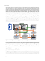
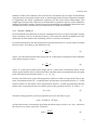
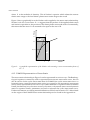
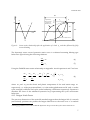
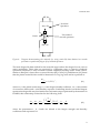
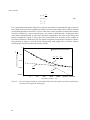
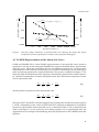
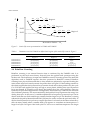
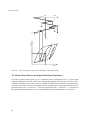
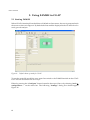
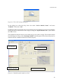
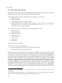
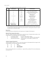

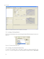
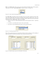
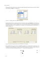

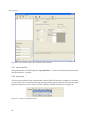
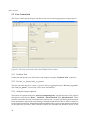
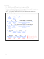
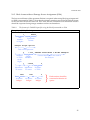
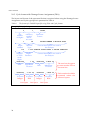
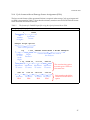
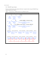
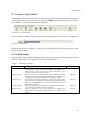
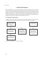
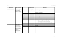
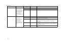
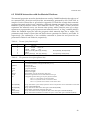
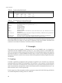
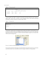
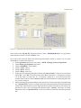
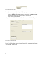
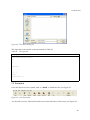
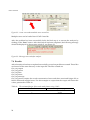
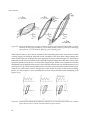


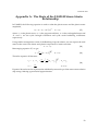

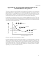
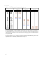
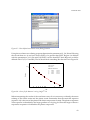
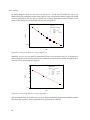
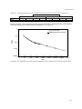

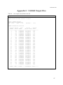
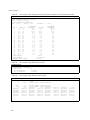
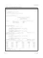
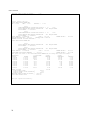
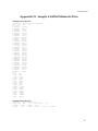

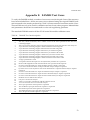
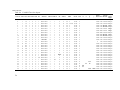
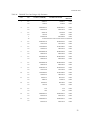
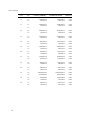


![Comment creuser un tunnel : méthodologie d`excavat[...]](http://vs1.manualzilla.com/store/data/006373896_1-46f0e6ba018fec4618d2bb7a5a678c3b-150x150.png)