Download Kinetic Logic Modeler: User Guide

Kinetic Logic Modeler: User Guide
Lukas Nick
August 13, 2010
Contents
1 About this Document
2
2 Requirements
2
3 Theoretical Background
3.1 Kinetic Logic Systems are Discrete . . . . . . . . . . . . . . .
3.2 Logical Functions: the Level in the Next Step . . . . . . . . .
3.3 Logical Parameter: a Weight for Each Term . . . . . . . . . .
2
3
4
5
4 How to Build a Model
4.1 Sketch your Model . . . . . . . . . . . . . . . . . . . . . . . .
4.1.1 Adding Concepts and Influences . . . . . . . . . . . .
4.1.2 Setting the Direction and Level of an Influence . . . .
4.1.3 Labeling the Levels of a Concept . . . . . . . . . . . .
4.1.4 Pure output concepts . . . . . . . . . . . . . . . . . .
4.1.5 The Model Window and the Concept Description Window . . . . . . . . . . . . . . . . . . . . . . . . . . . .
4.2 Define the K-Values . . . . . . . . . . . . . . . . . . . . . . .
4.3 Interpret the Output . . . . . . . . . . . . . . . . . . . . . . .
6
7
7
7
8
8
5 Saving, Opening and Describing
5.1 Saving a Model . . . . . . . . .
5.2 Opening a Saved Model . . . .
5.3 Add a Description to a Model .
6 The View Menu
8
9
11
a Model
13
. . . . . . . . . . . . . . . . . 13
. . . . . . . . . . . . . . . . . 14
. . . . . . . . . . . . . . . . . 14
14
7 The Help Menu
15
7.1 Switching Off the Help Bubbles . . . . . . . . . . . . . . . . . 15
8 References
15
1 About this Document
1
2
About this Document
This is a tutorial that explains some theoretical background of the Kinetic
Logic in the first part and in the second how to use the Kinetic Logic Modeler
(KLM). There we will develop a simple model using the KLM and interpret
its output.
2
Requirements
The Kinetic Logic Modeler (KLM) runs on Firefox (from version 2), Safari
(from version 5.0), Chrome (from version 5.0), Opera (from version 9), and
Internet Explorer — unfortunately only from version 8.0.
You need to enable Javascript in your browser.
To run KLM fluently, you need 1 GB of RAM.
3
Theoretical Background
The Kinetic Logic Modeler is a tool which models simple dynamic systems
based on “Kinetic Logic” (Thomas and D’Ari, 1990). This approach allows
modeling on an intermediate level between verbal description and nonlinear
differential equations.
Very often, a theory is about “things” and “how they influence each
other”. The things, here, are called “concepts”. The influences between
them are called, well, “influences”. If you manage to break down your theory
into such concepts and influences, you can sketch them and attach numbers
to the influences to describe how much one concept affects another one.
So you get a more formal model of your theory, and it becomes possible to
model impact, feedback and temporal evolution of the states of the concepts.
As the “system” (of concepts) evolves in time, one is able to detect resulting
attractors and to explore the effects that changes in the model might have on
the dynamics. So the Kinetic Logic Modeler is a tool which helps you think
about your theory. It was applied e.g. in biology to look into the dynamics
of infectious disease behavior (Martinet-Edelist, 2004) or in psychotherapy
research to examine the dynamics of psychotherapeutic interventions, their
effectiveness and sustainability (Kupper and Tschacher, 2006).
To illustrate some theoretical aspects and the use of the KLM, we will use
a simple psychological example, taken from Kupper and Tschacher (2006):
1. If a patient has impaired psychological health, he or she seeks psychotherapeutic treatment: an intervention.
2. The intervention increases the patients health.
3. If the health increases to a certain degree, the intervention stops.
3.1
Kinetic Logic Systems are Discrete
3
4. If the health is good enough, the patient is able to stay in a healthy
state (it is sustainable).
So, there are two concepts (intervention and health), some influences
between them, and ideas about the level from which these influences start
to become active (printed in italic and still quite fuzzy). In the following
sections, these ideas will be transformed into tangible terms.
3.1
Kinetic Logic Systems are Discrete
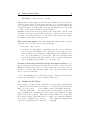
In contrast to other simulation tools, like e.g. Stella1 , which are based on
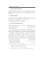
differential equations, KLM is a discrete system: concepts have discrete
levels (few, usually). The assumption is that a concept has no effect beneath a certain threshold v and its effect levels off above that threshold (see
Figure 1).
y
ef f ect
no ef f ect
x=0
v
x=1
x, continuous
x, discrete
Figure 1: The effect of the continuous variable x on another variable y
In our example, some psychotherapeutic intervention might have no noticeable influence on a patient’s health; only after the patient has gotten
a certain amount of intervention does his or her health change. Here, we
are only interested in the differentiation between has an influence and has
no influence on health: all other information about the relation between
influence and health we lose without regret.
So the continuous nature of an influence is reduced to discrete levels. A
concept has therefore as many levels as it influences other concepts, plus
one. In the example, intervention influences only health, so intervention
has the levels 0 (doesn’t influence health) and 1 (does influence health).
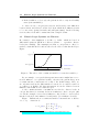
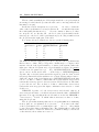
Figure 2 illustrates how a continuous variable x is turned into a discrete
one, x, by the function dx :

 0 if x ≤ v1 ,
1 if v2 < x ≤ v2 ,
x = dx (x) =
(1)

2 if v2 < x.
1
http://www.iseesystems.com/softwares/Education/StellaSoftware.aspx
3.2
Logical Functions: the Level in the Next Step
4
. . . where v1 and v2 are two thresholds (x, v1 , v2 ∈ R).
Such a (possibly multilevel) discrete variable is called logical variable in the
context of the Kinetic Logic.
0
v1
v2
x=0
x=1
x=2
x
Figure 2: The continuous variable x is discretized using thresholds v1 and
v2 .
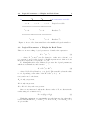
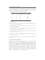
Boolean variables Then, for each
a set of Boolean variables, 1 x, 2 x,. . .
follows:
(
0
1
x=
1
multilevel logical variable x, there is
(see figure 3). E.g. 1 x is defined as
if x ≤ v1 ,
if x > v1 .
(2)
These Boolean variables are as Boolean as we expect them to be: they
have two values, 0 (for false) and 1 (for true).
3.2
Logical Functions: the Level in the Next Step
For each logical variable as defined above, there is a logical function 2 . They
denote the logical variable in the next step (at t + 1), and they are written
in capitals:
in usual notation:
in Kinetic Logic:
now:
time t
xt
x
next step:
time t + 1
xt+1
X
Logical functions describe the level towards which a logical variable
tends, e.g.
2
X=1
X=0
Tendency to show a certain behavior
No tendency to show the behavior
E.g. health will improve
E.g. health won’t improve
x=1
x=0
behavior is there
behavior is not there
E.g. good health
E.g. bad health
These are not functions in the mathematical sense.
Logical Parameter: a Weight for Each Term
v1
0
{
1
x=0
2
Logical variable
x=2
Boolean 1 x
x=0
{
1
x, continuous variable
x=1
{
x=0
v2
5
{
3.3
2
x=0
x=1
Boolean 2 x
Figure 3: A set of Boolean variables for the multilevel logical variable x.
3.3
Logical Parameter: a Weight for Each Term
There is one more thing: logical parameters. Consider the expression
X=
1
y ∨ 1z
(3)
. . . where X, 1 y, and 1 z are Booleans (i.e. either 0 for “absent” or 1
for “present”), and ∨ is the logical or. If this expression is 1, then we don’t
know if 1 y is present, 1 z is present, or both.
To distinguish such cases, Kinetic Logic uses the logical parameters,
which are real numbers, and rewrites (3) to:
X = K1 1 y + K2 1 z
(4)
. . . where X, K1 , K2 ∈ R and 1 y, 1 z ∈ {0, 1}. The term K1 t y has the value
0 or 1, depending on the value of the Boolean 1 y. So (4) is
0 if y and z are both absent,
K1 if only y is present,
K2 if only z is present,
K1 + K2 if both y and z are present.
Since we are interested only in the discrete value of X, we discretize the
result, using above function dx (1):
X = dx (K11 y + K21 z)
(5)
With this equipment, we can simulate several relations. Say x has three
levels, with thresholds v1 = 1 and v2 = 3. If we set K1 = 1.2 and K2 = 1.3,
we get an OR:
4 How to Build a Model
y
0
0
1
1
z
0
1
0
1
K1 1 y + K2 1 z
0
1.3
1.2
2.5
6
dx (K1 1 y + K2 1 z)
0
1
1
1
If we set K1 = 0.7 and K2 = 0.8, we get an AND:
y
0
0
1
1
z
0
1
0
1
K1 1 y + K2 1 z
0
0.7
0.8
1.5
dx (K1 1 y + K2 1 z)
0
0
0
1
If we set K1 = 1.2 and K2 = 1.9, we get a new relation:
y
0
0
1
1
z
0
1
0
1
K1 1 y + K2 1 z
0
1.2
1.9
3.1
dx (K1 1 y + K2 1 z)
0
1
1
1
In the KLM, the logical parameters are called K-values.
The next section explaines step by step how to make use of these theoretical ideas to create a model with concepts, define the influences between
them and examine their interplay—with the help of the KLM.
4
How to Build a Model
In this section we develop a model3 with the Kinetic Logic Modeler (KLM).
Before you start, you need to have an idea of your model, at least in your
head or in text form.Here is, again, our very simple psychological example:
1. If a patient has impaired psychological health, he or she seeks psychotherapeutic treatment: an intervention.
2. The intervention increases the patients health.
3. If the health increases to a certain degree, the intervention stops.
4. If the health is good enough, the patient is able to stay in a healthy
state (it is sustainable).
3
You can load the complete model we develop here by clicking “Load tutorial model”
in the help menu of the KLM.
4.1
Sketch your Model
7
The KLM consists of three tabs. The first to sketch your model, the
second to set the logical parameters (the K-values, see section 3.3), and the
third to view the output: a table showing the dynamics of the system.
4.1
Sketch your Model
When you load the page, you see the first tab where you can sketch the
model. To do this, use the two tools on the left of the screen: the concept
tool and the influence tool.
4.1.1
Adding Concepts and Influences
To add a concept, drag the concept tool into the canvas (the white area
that takes the biggest part of the screen). Release the mouse there: a new
concept is added to the model. Assign a name to the concept by clicking
into its only text field and writing “intervention” into it, then press enter.
Repeat this step and name the second concept “health”.
To add an influence, just click on the arrow tool on the left: the influence tool becomes blue, i.e. activated. Now move the mouse pointer over the
concept from which the influence is supposed to emanate (intervention, in
our case). You see that an arrow appears on the concept. Drag this arrow to
the concept that is supposed to be influenced by the first concept (health).
Release the mouse when you are over the target concept. The new influence
is drawn as an arrow between the two concepts (and the influence tool is
deactivated). This influence represents the second phrase of above verbal
description of our model: an intervention increases the patient’s health.
4.1.2
Setting the Direction and Level of an Influence
To indicate that the influence increases health, we have to set the direction
of the influence. To do this, click on the link “?/+” in the box attached
to the arrow. This opens a dialog box, where you can define whether the
influence is activating or inhibiting. Click on “activating”. Next, we have
to define from which level of intervention the influence becomes active.
Choose 1 — the only option available now, since there is only one influence
emanating from intervention.
Next, draw another influence, from health to intervention. Set this
influence to inhibiting and its start level to 1 (again the only option available
for now). It represents the third phrase of the verbal description: good
health stops the intervention.
To represent the last phrase of the model (sustainable health), we need
another influence from health to itself. Click on the influence tool, move the
mouse to the health concept, start dragging the arrow-symbol away from
the concept and back to it, release the mouse when the pointer is again
4.1
Sketch your Model
8
on the concept: an arrow is created that starts from health and ends on it.
Click on the “?/+”-box, choose “activating” and 2 beneath “Influence starts
if level of “health” is at least...”. This means that health is self sustainable
only when it has reached the second level.
4.1.3
Labeling the Levels of a Concept
Each concept has as many levels as it influences other concepts, plus 1. You
can attach labels to these levels: click on “labels” in the upper right corner
of a concept symbol to open the labeling dialog and enter a name for each
level.
Label the two levels of intervention: “absent” for 0 and “present” for 1.
Label the three levels of health: “bad” for 0, “moderate” for 1, and “good”
for 2.
4.1.4
Pure output concepts
Within the framework of Kinetic Logic, a concept that doesn’t influence any
other concept (and neither itself; a “pure output concept”) is of no use: since
each concept has as many levels as it influences other concepts, plus one,
such a concept would have 0 + 1 = 1 levels, and this one level would always
be 0. I.e. this concept would always stay in the same state, 0, regardless of
what is happening in the simulation.
There might be situations, though, were you want to model such a pure
output concept. To accomplish this, create the concept and draw an additional influence from this concept back to itself. Set the level of this
self-referencing incluence to 1 and its direction to “activating”.
This construct probably doesn’t make any sense in terms of your theory;
it is just a workaraound to circumvent a constraint of Kinetic Logic. Therefore, to neutralize the theoretically useless meaning of the self-reference,
you need to set the according K-values in the K-value table to zero (see
section 4.2).
4.1.5
The Model Window and the Concept Description Window
There are two small windows at the bottom border of the screen: one showing a mathematical description of the model and one showing a textual
description of the concepts.
You can shift them around on the screen if you grab their grey title bar
with the mouse and drag them.
The model description The mathematical description of the model has
the title “Model”; at this point, it shows this:
IN T ERV EN T ION = 1 health
4.2
Define the K-Values
HEALT H =
1 intervention
9
+ 2 health
This means, the intervention in the next step will increase if the negation
of the Boolean variable 1 health is true (the line above health means “negation”). That is, intervention will increase if health is 0 and it is inhibited if
health is at least 1. To which value intervention will increase, we are going
to define on the next tab when we set the K-values.
Similarly health in the next step will increases if the sum of the Boolean
variables 1 intervention and 2 health is at least 1 . That is, if intervention is
at least 1 or health is at least 2, or both, then health will increase. Again,
how much, we will define on the next tab.
The concept description The other small window has the title “Concept
description”: it describes each concept by showing. . .
• the name of the concept,
• a sentence for each influence emanating from the concept. This sentence describes the influence the concept has on the target concept,
that is, whether it is activating or inhibiting and from which level of
the concept the influence becomes active. The level description uses
the label we defined in the labels dialog of the concepts, and it shows
the level number in parentheses, e.g. “moderate (1)”.
To hide or show the model and concept description windows, use
the according menu items from the menu “View” in the top most bar of the
KLM. If you just want to hide one of these windows, you can also click on
the little “x” in the window’s upper right corner. To show it again, you’ll
have to use the View menu.
As soon as all influences are defined properly (i.e. their direction and level
set), the tab “K-Values” becomes activated. Click on it.
4.2
Define the K-Values
Next, we have to define for each combination of levels of the logical variables
to which level they tend in the next step (i.e. to define the logical functions).
Have a look at section 3.2 if you are unsure what logical functions mean.
The important thing on the current page is a table with two parts. The
left part displays all combinations of levels of the logical variables (column
titles in lower case caption). This is an ordinary truth table, except that
there maybe values other than 0 and 1, because logic variables in Kinetic
Logic may be multilevel (see section 3.1). The right part displays their
respective logical functions (column titles in capitals).
4.2
Define the K-Values
10
The two windows with the model description and the concept description
are arranged on the left side (because the table can become large if the model
has many concepts).
In the theoretical description above (section 3.2), in order to define the
value of the logical function, we had to first set K-values and then discretize
the result (using the function dx (1)). Now, in contrast to this, we do these
two steps in one: we directly define the level of the logical variable in the
next step (i.e. the level of the logical function) by choosing a number from
the dropdown in the right part of the table.
For our model, as we defined it so far, we get the following table:
Logical Variables
intervention health
0
0
0
1
0
2
1
0
1
1
1
2
Logical Functions
INTERVENTION HEALTH
15
0
0
0
0
15
15
15
0
15
0
15
The numbers with the triangles (5) are those outputs of the logical functions
that we have to define. They correspond to situations (i.e. to input combinations of levels of the logical variables, or “states of the system”) where the
right part of the model equation for a logical variable is 1 (true; an example
for such a model equation is eq (5)). E.g. IN T ERV EN T ION = 1 health
(as we can see in the model window on the left), so IN T ERV EN T ION
depends only on health; it increases if the negation of the Boolean 1 health
is 1 (true), that is if health is neither 1 nor 2, but 0. That is why we have to
define the output of the logical function for IN T ERV EN T ION in the first
row. I.e. we have to define to which value the logical variable intervention
tends in the next step given both intervention and health are 0. The same
goes for the 4th row: here we have to define to which value intervention
tends in the next step given the input combination intervention = 1 and
health = 0.
HEALT H depends on both 1 intervention and 2 health, that is, if
intervention is at least 1 or health is at least 2, then the value of HEALT H
increases. You can read this in the model window on the left: HEALTH =
1 intervention + 2 health. To which value it increases, we have to define,
using the dropdown.
The dropdown has as many values as a concept has influences emanating
from it, plus one, as explained above (section 3.1). You can set the value
of the logical function for a certain input combination to 0 — there might
be rare cases where this would make sense. The default value for all logical
functions we have to define is 1. Whenever you make a change to the model
on the first tab, these values are reset to 1.
4.3
Interpret the Output
11
Let’s set the K-values for our model. To do this, we have to use the verbal
description of a given theory. So the following K-values are just one possible
solution that seems to make sense in this example:
Logical Variables
intervention health
0
0
0
1
0
2
1
0
1
1
1
2
Logical Functions
INTERVENTION HEALTH
15
0
0
0
0
25
15
15
0
25
0
25
Explanations:
1th row: health is bad, so the patient gets an intervention (intervention is
present (1) in the next step).
3th row: health is good (2), so it should stay so even if there’s no intervention (self sustainable).
4th row: health is bad, so the patient gets an intervention. The intervention
increases health to moderate (1).
5th row: A present intervention combined with a moderate level of health
increases health to good (2).
6th row: The good health is self sustainable (the ongoing intervention doesn’t
matter anymore).
Having set all K-values, we can proceed to the third tab to read the output
of the model.
4.3
Interpret the Output
This page shows a state table representing the output of the modeling: the
dynamics of the model. If a model has only two concepts, this table can
be read as a state space where each dimension axis represents the levels of
a concept. The combination of the levels of all concepts - the state of the
system - is a point in this space. In our case we have intervention on the
horizontal axis and health on the vertical axis (see table 1). Both axes are
not continuous; they show the levels of their concept, using the (abbreviated)
level labels of the concepts, if defined, and the level number in parentheses.
If there are more than two concepts in the model, this table is nested and
cannot be easily interpreted as a state space anymore.
4.3
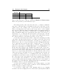
Interpret the Output
Health
good(2)
moderate(1)
bad(0)
02
01
00
absent(0)
12
11
10
present(0)
12
Intervention
Table 1: The state space of the two dimensions Health and Intervention.
Each cell represents a point in this state space.
The numbers in the cells of the table show the “coordinates” within the
state space. The first digit of each number is the level of the first concept.
(“first” refers to the ordering of the concepts in the model view window).
The second digit is the level of the second concept, and so on. For example
the lower left cell has the number 00 which means it represents the situation
(the “state”) where intervention = 0 and health = 0. Similarly, the upper
right cell with the number 12 represents the state where intervention = 1
and health = 2. So this table shows all entries of the left part of the Kvalues table on the second tab (i.e. the entries of the truth table), but here
the cells are arranged on axes that represent a concept, each.
A cell, then, represents a state at time t. The arrow emanating from this
cell points to the state at the next step, t+1. This corresponds to the logical
function we defined in the K-values table. But there is one difference: in
Kinetic Logic, only one concept can change at a time. This means that there
are no diagonal arrows in the state table. Consider the 5th row in the Kvalue table: intervention = 1 and health = 1, and the output of the logical
functions for this input is IN T ERV EN T ION = 0 and HEALT H = 2.
In the state table (again on the dynamics tab), this would correspond to
an arrow from the middle right cell 11 to the upper left cell 02 if both
intervention and health could change at the same time (from 1 to 0 and
from 1 to 2, respectively). But this is not allowed. Instead, in the cell 11,
either intervention can change from 1 to 0, resulting in the new state 10,
or health can change from 1 to 2, resulting in the state 12. These two
possibilities are represented on the one hand by two arrows emanating from
the cell 11 and on the other hand by the tiny red minus resp. plus signs
above the digits of the cell number (− and + ): they indicate which concept is
going to change in the next step and into which direction. So the behavior of
the system can fork in this state. Which path it takes, is something beyond
the KLM: it cannot be modeled using Kinetic Logic.
A stable state is marked by inverted colors: a white number on a dark
background. Moreover, such a stable cell has no arrows emanating from it
and, accordingly, no minus or plus signs.
So let us try to make sense of the dynamics table we got: Starting
from the lower left cell (00), there is no intervention (absent) and health is
5 Saving, Opening and Describing a Model
13
bad. This leads the intervention to start (i.e. to be present) in the next
state whereas health is still bad (arrow to the right into cell 10). But the
present intervention increases the health in the next step to moderate (arrow
upwards to 11). Now the system could take two paths (a fork): on the first
path, the intervention stops (because good health decreases the motivation
for intervention (see the third point of the verbal description of our theory,
section 4), leading to the state 01. Since the health is not on a self sustainable
level, it drops back to bad, so the next state is 00 — were we started. What
we see is a cyclical attractor.
But there is another path starting in the state 11: if the intervention
doesn’t stop, health increases to its self sustainable level “good” (2, state
12) and from there, since good health stops the intervention, we end up in
the state 02. This is a stable state, i.e. a point attractor, because good
health is self sustainable and intervention is only triggered if health is bad.
You can drag the cells of the state table; this can help to get a better
view of the dynamics if there are many concepts with many arrows.
Now, play with the model and see what happens with the dynamics.
How do the dynamics change if a present intervention and a moderate health
don’t push health up to good but only keep it on moderate? To test this,
you have to set the K-value for health in the 5t h row of the K-values table
to 1 instead of 2. What happens if the inhibiting influence from health to
intervention becomes active only from level 2 (good health) instead of from
level 1 (moderate health)?
5
Saving, Opening and Describing a Model
You can save a model, including its K-values, to a text file, load a model
from a text file, and attach a description to a model.
5.1
Saving a Model
To safe a model:
• Click on the menu “Model” and choose the menu item “Save”. This
opens a dialog box with one big text field. In this text field there is a
coded representation of the model you created so far.
• Select all text in this text field. To do this, you can click on the button
“select all”, or mark it with your mouse, or press “ctrl-a” if the writing
cursor is inside the text field.
• Copy it into your clipboard. Use the key combination “ctrl-c” or, on
a mac, “apple-c”. Alternatively you can right click into the text field
and choose “copy” from the right-click-menu.
5.2
Opening a Saved Model
14
• Now open a file in a text editor that allows to edit plain text (like
Notepad on Windows, or SimpleText on a mac), and paste the code
you just copied into that file. Use the key combination “ctrl-v” on
Windows and Linux, “apple-v” on a mac, or use the paste command
from the edit menu.
• Save this file somewhere where you can find it again. . .
Saving a model includes the concepts with their level labels, the influences with their direction and level, the K-values and the description of the
model.
5.2
Opening a Saved Model
To open a model you saved earlier (using the procedure just described):
• Click on the menu “Model” and choose the menu item “Open”. If you
have already started to sketch a model, a warning message appears:
Opening a new model discards whatever is currently in the KLM. If
you confirm, a dialog box shows up with a big text field.
• Open the file on your hard disk where you saved the model (section
5.1), select all text in the file and copy it to the clipboard.
• Paste this into the big text field.
• Click the button “ok”.
5.3
Add a Description to a Model
To add a description to your model:
• Click on the menu “Model” and choose the menu item “Description”.
This opens a dialog box.
• Enter the author (probably you), a date and a version, and a description of your model: there you might want to state the verbal
description of the theory you want to model, or any other notes.
• Click on the button “ok” to accept the description. This doesn’t save
the description! Only when you save the model to a text file as described above (section 5.1) a model is saved including its description.
6
The View Menu
The View menu allows you to hide and show the model window and the
concept description window. If they are visible, you can hide them, if they
7 The Help Menu
15
are closed, you can show them. You can hide each window also by clicking
on the “x” in its upper right corner. Then you have to use the View Menu’s
show command to reopen it again.
7
The Help Menu
The Help menu has three entries: one to switch off the help bubbles, one to
display or download this tutorial, and a third to show an about box.
7.1
Switching Off the Help Bubbles
Hovering the mouse pointer over certain User interface elements of the KLM
screen displays a green bubble with a hint that is supposed to help you
understand the element. If you are tired of these bubbles, you can switch
them off by clicking on “Switch off help bubbles” in the Help menu. This
entry changes now to “Switch on help bubbles”. You have to click it to see
them again.
8
References
Kupper, Z. and Tschacher, W. (2006). Anwendung - Effektivit¨at Aufrechterhaltung. Boolesche Interventionsmodelle zur Wirkung von Psychotherapie. Zeitschrift f¨
ur Klinische Psychologie und Psychotherapie,
35(4):267–285.
Martinet-Edelist, C. (2004). Kinetic logic: a tool for describing the dynamics
of infectious disease behavior. J. Cell. Mol. Med., 8(2):269–281.
Thomas, R. and D’Ari, R. (1990). Biological Feedback. CRC Press, Boca
Raton.