1
NENOK 1.1 User Guide∗
Marc Pouly
Department of Informatics
University of Fribourg
CH – 1700 Fribourg (Switzerland)
http://diuf.unifr.ch/tcs/
January 30, 2006
Abstract
NENOK is a distributed software framework written in Java that provides
an experimental workbench for users interested in local computation. Thereby,
they can realize own valuation algebra instances based on a framework structure
that reflects the algebraic background of this theory. NENOK allows then to
apply various local computation architectures on knowledgebases that are made
up of such user objects. In particular, these objects may even be spread over a
network and are consequently processed in a distributed manner. Furthermore,
the underlying join tree structure of local computation can be inspected and
manipulated in different ways. All this is driven by a very simple and intuitive
interface with the central philosophy that the call of the NENOK framework
should not take more than three lines of code.
∗
Research supported by grant No. 20-67996.02 of the Swiss National Foundation for Research.
CONTENTS
2
Contents
1 Introduction
4
1.1
Mission . . . . . . . . . . . . . . . . . . . . . . . . . . . . . . . . . .
4
1.2
Naming & Versioning
. . . . . . . . . . . . . . . . . . . . . . . . . .
4
1.3
Technical Aspects & Notation . . . . . . . . . . . . . . . . . . . . . .
5
1.4
Organization . . . . . . . . . . . . . . . . . . . . . . . . . . . . . . .
5
2 Introduction to Jini
2.1
2.2
6
Jini Components . . . . . . . . . . . . . . . . . . . . . . . . . . . . .
6
2.1.1
Jini Services . . . . . . . . . . . . . . . . . . . . . . . . . . . .
6
2.1.2
Jini Clients . . . . . . . . . . . . . . . . . . . . . . . . . . . .
7
Support Services . . . . . . . . . . . . . . . . . . . . . . . . . . . . .
8
3 The NENOK Architecture
10
4 The Valuation Algebra Framework
11
4.1
4.2
4.3
Valuation Algebra Core Components . . . . . . . . . . . . . . . . . .
12
4.1.1
Variables . . . . . . . . . . . . . . . . . . . . . . . . . . . . .
12
4.1.2
Domains . . . . . . . . . . . . . . . . . . . . . . . . . . . . . .
13
4.1.3
Valuations . . . . . . . . . . . . . . . . . . . . . . . . . . . . .
13
4.1.4
Identity Elements . . . . . . . . . . . . . . . . . . . . . . . . .
16
4.1.5
Printing Valuation Objects . . . . . . . . . . . . . . . . . . .
16
Extended Valuation Algebra Framework . . . . . . . . . . . . . . . .
18
4.2.1
Valuation Algebras with Division . . . . . . . . . . . . . . . .
18
4.2.2
Scalable Valuation Algebras . . . . . . . . . . . . . . . . . . .
19
4.2.3
Idempotent Valuation Algebras . . . . . . . . . . . . . . . . .
20
4.2.4
Weight Predictable Valuation Algebras . . . . . . . . . . . . .
20
Semiring Valuation Algebra Framework . . . . . . . . . . . . . . . .
22
4.3.1
Finite Variables . . . . . . . . . . . . . . . . . . . . . . . . . .
23
4.3.2
Semiring Elements . . . . . . . . . . . . . . . . . . . . . . . .
23
4.3.3
Semiring Valuations . . . . . . . . . . . . . . . . . . . . . . .
24
4.3.4
Regular Semiring Valuations & Scaling . . . . . . . . . . . . .
25
CONTENTS
3
5 Case Study: Probability Potentials
5.1
Probability Potentials in Action . . . . . . . . . . . . . . . . . . . . .
6 Remote Computing
27
28
30
6.1
Processor Networks . . . . . . . . . . . . . . . . . . . . . . . . . . . .
30
6.2
Remote Valuation Objects . . . . . . . . . . . . . . . . . . . . . . . .
32
6.3
Knowledgebase Registry . . . . . . . . . . . . . . . . . . . . . . . . .
33
6.4
Remote Valuation Algebra Operations . . . . . . . . . . . . . . . . .
35
7 Running a NENOK Federation
38
7.1
HTTP Server . . . . . . . . . . . . . . . . . . . . . . . . . . . . . . .
39
7.2
Reggie . . . . . . . . . . . . . . . . . . . . . . . . . . . . . . . . . . .
39
7.3
Knowledgebase Registry . . . . . . . . . . . . . . . . . . . . . . . . .
39
7.4
Starting a NENOK application . . . . . . . . . . . . . . . . . . . . .
40
8 Local Computation
40
8.1
Local Computation Factory . . . . . . . . . . . . . . . . . . . . . . .
41
8.2
Join Trees & Local Computation . . . . . . . . . . . . . . . . . . . .
41
8.3
Architectures of Local Computation . . . . . . . . . . . . . . . . . .
42
8.4
Join Tree Construction Algorithms . . . . . . . . . . . . . . . . . . .
44
9 Generic Input
49
9.1
Knowledgebase Input Files
. . . . . . . . . . . . . . . . . . . . . . .
49
9.2
Join Tree Input Files . . . . . . . . . . . . . . . . . . . . . . . . . . .
54
10 Graphical User Interface
57
11 Conclusion & Future Work
59
References
61
1 Introduction
1
4
Introduction
Local computation techniques were originally introduced for probability networks
by (Lauritzen & Spiegelhalter, 1988). They provided a solution for a problem that,
without this approach, would be computationally intractable. Over the following
years, a lot of research was dedicated to widen these techniques on other formalisms.
A first generalization has been proposed by (Shenoy & Shafer, 1990) basically held
up by a set of axioms that were sufficient for local computation. This was the hour of
birth of an abstract algebraic structure called valuation algebra (Kohlas & Shenoy,
2000; Kohlas, 2003) that underlies local computation. Until this day, many different
valuation algebra instances are known and a representable collection can be found in
(Kohlas, 2003). The recent work of (Schneuwly et al., 2004) assembles the current
state of research and constitutes the theoretical basis of a software framework called
NENOK whose description is the scope of this paper.
This paper describes the buildup and functionality of the NENOK software
framework such that users are able to realize their own projects upon it. We will
report all important components and illustrate their use by examples. Particularly,
we give detailed insights into the algebraic framework part and provide a user guide
for its instantiation. Furthermore, this paper should support the user in launching
a NENOK environment and point out the classical pitfalls of configuration.
1.1
Mission
The NENOK software project aims at providing a complete generic implementation
of local computation theory. Its core is constituted of an abstract representation
of the valuation algebra framework upon which the architectures of local computation and related concepts are implemented. A central point in the development of
NENOK is to respect the distributed nature of information. Therefore, it is designed
as a distributed framework that allows to process valuation objects that reside on
different hosts of a common network.
1.2
Naming & Versioning
In Persian mythology, Nenok names the ideal world of abstract being. According to
the Iranian prophet Zarathustra, the world was first created in an only spiritual form
and named Nenok. Three millenniums later, its material form named Geti finally
accrued. Because the whole theory of local computation grounds on the abstract
valuation algebra framework, we chose the name NENOK to act for this software
project.
A first step in the development of the NENOK framework was done in (Pouly,
2004) and provided a purely local implementation based on a very restricted algebraic framework. The current NENOK 1.1 release covered by this paper is constituted of a new communication layer and an extensive algebraic part such that
1.3
Technical Aspects & Notation
5
backward compatibility could hardly be preserved. Nevertheless, we claim that instances based on the former NENOK version are convertible with only small effort
to this new and more powerful version.
1.3
Technical Aspects & Notation
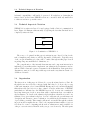
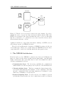
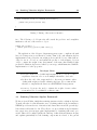
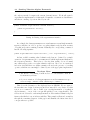
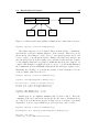
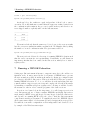
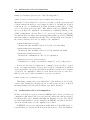
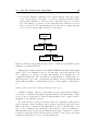
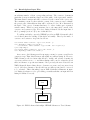
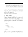
NENOK 1.1 is written in Java 1.5.0 and equipped with a Jini 2.0 communication
layer. Figure 1.1 illustrates this assembly by ignoring the fact that Jini itself is not
completely written in Java.
NENOK
Jini
Java
Figure 1.1: Constitution of NENOK 1.1.
The source code printed in this paper is written in pure Java 1.5.0 but for the
sake of simplicity and clarity we will set dispensable details aside. Typically, most
of the exception handling procedure will be omitted throughout this paper as well
as package imports, main method definitions, etc.
The comprehension of the internal class structure and component interaction is
inalienable for users that wish to implement own valuation algebra instances and we
will use UML 2 class and sequence diagrams for their illustration. But again, these
diagrams are narrowed on the important aspects in such a way that irrelevant code
details are left aside.
1.4
Organization
The first section of this paper is dedicated to a very short introduction of Jini. Although the user is not directly confronted with Jini related code, he needs to set up
a Jini environment in order to start NENOK. Having an idea about Jini will simplify
this task notably. In Section 3 we have a first look at the architecture of NENOK;
particularly we will introduce the NENOK layer model. Section 4 is certainly the
most important part for those users that wish to implement their own valuation
algebra instance. It describes the valuation algebra framework and how it can be instantiated for a given valuation algebra. Section 5 will pause the general framework
description and discuss a concrete realization of a valuation algebra instance by use
of probability potentials. This example will attend our studies through the remaining sections and exemplify the use of the local computation functionalities. Section 6
is dedicated to remote computing and shows how valuations are made available for
other processors in a network and how they are processed remotely. The subsequent
2 Introduction to Jini
6
section contains a step-by-step tutorial on running a complete NENOK environment including the underlying Jini services. Based on all these concepts, section 8
describes the application of local computation techniques such that the user will
receive an impression on the power of NENOK. Another important framework part
is described in section 9 and provides a system for generic input processing. Closing,
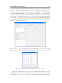
we get a glimpse of a graphical experimental workbench for local computation that
is shipped with the current NENOK release.
2
Introduction to Jini
Jini is a distributed computing environment provided by Sun Microsystems that
offers network plug and play. Thereby, a device or a software service can connect to
an existing network and announce its presence. Clients that wish to use this new
service can locate it and call its functionality. New capabilities can be added to a
running service without disrupting or reconfiguring it. Additionally, services can
announce changes of their state to clients that currently use this service. This is in
a few words the principal idea behind Jini.
2.1
Jini Components
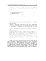
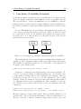
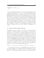
A Jini system or federation is a collection of clients and services that communicate
by the use of the Jini protocol. Basically, there are three main players involved:
services, clients and the lookup service that acts as a broker between the former two.
Client
Lookup Service
Service
Network TCP / IP
Figure 2.1: The three main players of a Jini system.
2.1.1
Jini Services
Services are logical concepts commonly defined by a Java interface. A service
provider disposes of an implementation of the appropriate interface and creates
service objects by instantiating this implementation. Then, the service provider
contacts the lookup service in order to register its service object. This is done either directly by a unicast TCP connection or by UDP multicast requests. In both
2.1
Jini Components
7
cases, the lookup service will answer by sending a registrar object back to the service
provider. This object now acts as a proxy to the lookup service and any requests
that the service provider needs to make of the lookup service are made through this
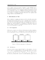
registrar. Figure 2.2 illustrates this first handshake between service provider and
lookup service.
Lookup Service
Service Provider
1
Service
Object
2
Registrar
Figure 2.2: Contacting a lookup service is a two-step procedure. The lookup service
is first located and then a registrar proxy of the lookup service is stored on the
service provider.
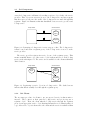
The service provider registers its service by use of the registrar proxy. This
means essentially that a copy of the service object is taken and stored on the lookup
service as shown in figure 2.3. The service is now available for the clients within this
Jini federation.
Lookup Service
Service Provider
Service
Object
Service
Object
Registrar
Figure 2.3: Registering a service object in a lookup service. The dashed arrows
indicate that this is actually done through the registrar proxy.
2.1.2
Jini Clients
The necessary procedure for clients to use an exported service is almost mirrorinverted. They contact on their part the lookup service and get in response a
registrar object. Then, the client asks the lookup service through the registrar
proxy for an appropriate service object that implements the needed functionality. A
copy of the service object is then sent to the client and the service is available within
2.2
Support Services
8
the client’s virtual machine. Figures 2.4 and 2.5 illustrate how clients request for
services.
Client
Lookup Service
1
Service
Object
2
Registrar
Figure 2.4: The procedure of contacting a lookup service is essentially the same for
both clients and service providers.
Client
Lookup Service
Service
Object
Service
Object
Registrar
Figure 2.5: Through the proxy, the client asks the lookup service for a service object
that is transmitted afterwards to the client’s virtual machine.
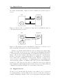
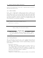
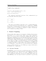
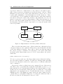
Until now, we silently assumed that the service is built up from a single, lightweight object. This object is exported to a lookup service and transmitted afterwards
to all clients interested in its functionality. For sophisticated applications however,
this procedure is barely adaptive. Especially services designed to control hardware
should be local on the corresponding machine, not to mention the colossal database
service that would be transmitted over the network. Instead of a single service
object, we prefer to have at least two, one lightweight proxy object running in the
client and another distinct one running in the service provider. This is illustrated
in figure 2.6. The client uses the service by calling the service proxy, which in
turn communicates with its implementation on the service provider. This additional
communication is indicated in figure 2.6 by the dashed double-arrow.
2.2
Support Services
We have seen so far that Jini relies heavily on the ability to move objects from
one virtual machine to another. This is done by the use of the Java serialization
technique. Essentially, a snapshot of the object’s current state is taken and serialized
2.2
Support Services
9
Lookup Service
Client
Service
Proxy
Service Provider
Service
Proxy
Service
Impl
Registrar
Registrar
Figure 2.6: In order to prevent the transmission of a huge service object, we divide it
up into a service proxy and a service implementation. The proxy is transmitted over
the network and communicates with its implementation that is local to the service
provider’s virtual machine.
to a sequence of bytes. This serialized snapshot is moved around and brought back
to life in the target virtual machine. Obviously, an object consists of code and data,
which both must be present to reconstruct the object on a remote machine. The data
part is represented by the object snapshot but we cannot assume that every target
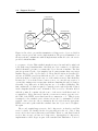
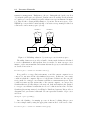
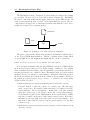
machine disposes of the object’s class code. Every Jini federation encloses therefore
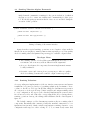
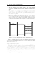
at least one HTTP server from which the needed code can be downloaded. This
is shown in figure 2.7 and by the way one of the main reasons for Jini’s flexibility.
Because the code is fetched from a remote server, one can add new services or
even modify existing services at any time without relaunching the whole federation.
Generally, every Jini service is divided up into two code archives (JAR files). The
first contains all code that is required to start the service and is typically declared
in the classpath when the service is launched. The second, by convention labeled
with the postfix dl, contains only the source of the service itself that is used for
reconstruction. Every Jini service has the java.rmi.server.codebase property set to
the URL of the HTTP server that hosts its reconstruction code. This property
is assigned to the serialized service whenever it needs to be transmitted over the
network. On receiver site, the reconstruction file is loaded from the appropriate
HTTP server and together with the serialized data, the object can be brought to
life again.
The second essential support service, the lookup service, is already a real Jini
service by itself. We discussed in the foregoing subsection the role of the lookup
service as a broker between Jini services and clients. Therefore, each Jini federation
needs to have access to at least one lookup service. Sun supplies a lookup service
implementation called Reggie as part of the standard Jini distribution. Section 7
3 The NENOK Architecture
10
HTTP Server
Client
Cod
service-dl.jar
e
Service
Service Provider
ta
+ ase
b
de
Co
Da
Service
service.jar
Figure 2.7: The file service.jar is used to start a new service instance. In order to
transmit the service object to the client, its data is serialized and the URL of the
HTTP server is attached. The client deserializes the service object by downloading
first the reconstruction code contained in service-dl.jar from the webserver whose
address is known from the codebase.
explains in detail how to setup a Jini environment consisting of a HTTP server as
well as Reggie as part of a NENOK federation.
The next section will start the description of NENOK by giving a global view
on its architecture. This is done by introducing the NENOK layer model whose
components will be described in detail throughout the subsequent sections.
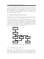
3
The NENOK Architecture
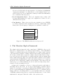
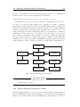
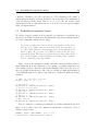
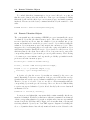
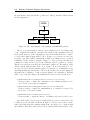
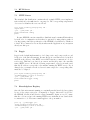
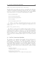
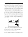
From the bird’s eye view, NENOK is constructed as a layer model illustrated in
figure 3.1. Each of its five layers benefits from the functionality of its underlying
neighbor and attends only to the tasks related to itself. In a nutshell, the task of
each layer is summarized is follows:
• Communication Layer: The lowest layer establishes the communication
utilities which are for the most part provided by the use of the Jini framework.
• Valuation Algebra Layer: This layer contains the abstract framework to
represent the underlying algebraic structure of local computation. It is built
upon the communication layer such that valuations are serializable objects
which can be transmitted over the network.
• Remote Computing Layer: Provides services to store valuation objects in
globally shared memory spaces in order to make them accessible for clients in
4 The Valuation Algebra Framework
11
the network. Additionally, the implementation of a (distributed) COMMAND
design pattern (Gamma et al., 1993) allows to execute valuation algebra operations on remote processors. Furthermore, this layer realizes the mathematical
idea of distributed knowledgebases.
• Local Computation Layer: The local computation layer consists of all
necessary implementations to apply local computation on either a local or
distributed knowledgebase.
• User Interface: This top layer provides a more intuitive access to NENOK
by default configurations and a graphical user interface. Additionally, a small
framework for generic input processing has been established on this level.
Local Computation Layer
Remote Computing Layer
NENOK
User Interface
Communication Layer
Jini
Valuation Algebra Framework
Figure 3.1: The NENOK architecture as a layer model.
4
The Valuation Algebra Framework
The valuation algebra framework is the central part of NENOK for those people
that want to implement their own valuation algebra instance. The mathematical
definition of a valuation algebra given in (Schneuwly et al., 2004) consists of various
components such as variables, domains, valuations and identity elements which are
all correlated. Additionally, we may have valuation algebras with division, idempotency and other properties and there are further structures such as semirings that
induce valuation algebras. This section guides through the realization of these mathematical structures in NENOK and describes the measures that need to be taken by
the user in order to implement a valuation algebra instance. Most subsections end
with developer notes which summarize in a few words the most important points to
remember for the programmer at work.
A framework is essentially a collection of classes and interfaces with tight relationships among each others. In our jargon, implementing a valuation algebra
instance is a synonym for extending and implementing NENOK classes and interfaces for a given mathematical formalism that has proven to be a valuation algebra
instance. Therefore, it is indispensable to become acquainted with every component
of NENOK’s valuation algebra layer, to study their interplay and to be sure of their
mathematical counterpart. This is the outline of the current section.
4.1
Valuation Algebra Core Components
12
4.1
Valuation Algebra Core Components
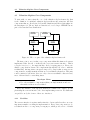
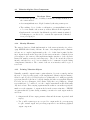
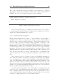
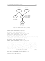
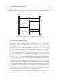
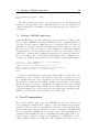
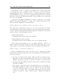
To start with, we survey first the core of the valuation algebra framework, that
is, the definition of a standard valuation algebra without any extensions. All Java
components that are directly involved in this definitions and their relationships are
shown in figure 4.1. The two shadowed interfaces do not belong to NENOK but are
part of the standard Java distribution.
interface
Cloneable
interface
Serializable
interface
Valuation
interface
Variable
*
1
Identity
Domain
Figure 4.1: The core part of the valuation algebra framework.
The first point to note is that every component within this framework extract
implements either directly or indirectly the java.io.Serializable interface. This is
a marker interface, i.e. an empty interface used for typing purposes. Every serializable component in Java needs to implement this interface in order to mark its
serializability. An important consequence imposed by Java is that we may not use
components in our implementations that are not serializable themselves. This may
sound constrictive but in fact, there are only a few non-serializable classes in Java,
most of them related to networking issues.
Developer Notes
• Use only serializable components within your implementation and note
that static fields are never serialized.
Every user instance of the algebraic framework consists of two classes, one implementing the Variable interface, the other implementing Valuation. We shall start
our guided tour by the former of these two interfaces.
4.1.1
Variables
The Variable interface is again a marker interface, but nevertheless, there are some
important remarks concerning its implementation. Every Java component is a descendant from the root component java.lang.Object, which provides a set of default
4.1
Valuation Algebra Core Components
13
methods that are frequently used by other components. These methods need to be
personalized:
• public boolean equals(Object o);
According to the mathematical background, variables are collected within domains and therefore should be distinguishable from one another. The preimplementation of this equality check compares the memory address of the
involved objects. This must be changed to an implementation based on the
variable’s content rather than its memory address.
• public int hashCode();
As we will see, NENOK represents domains as hash sets of Variable objects. In
order to guarantee their efficient and correct arranging, the user should ensure
a reasonable implementation of this hash code function.
• public String toString();
Printing the computation’s result is naturally an important task in NENOK
which will be addressed in more detail at the end of this section. Nevertheless, we advise to the user to overwrite this string conversion by a suitable
representation of the current variable.
Developer Notes
• Make sure that your Variable implementation overwrites the equals,
hashCode and toString methods inherited from java.lang.Object.
4.1.2
Domains
Domains, as shown in figure 4.1, are essentially sets of Variable objects. Internally,
they are implemented as hash sets that offer constant time performance for most
basic set operations such as add, remove, contains and size. But this assumes that
the Variable implementation is equipped with a hash function that disperses the
elements properly among the buckets. Apart from this, it is an implementation of a
simple set type with all typical set operations.
4.1.3
Valuations
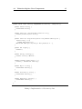
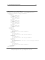
The Valuation interface is the lion’s share of a valuation algebra implementation. Its
source code is given in listing 1. The three methods at the head named label, combine
and marginalize represent their mathematical namesakes defining a valuation algebra.
Furthermore, this interface contains a method to compute a valuation’s weight and
allows to create clones of its instances.
• public Domain label();
The labeling method returns the domain of a valuation object.
4.1
Valuation Algebra Core Components
14
public i n t e r f a c e Valuation extends Serializable , Cloneable {
public Domain label ( ) ;
public Valuation combine ( Valuation val ) ;
public Valuation marginalize ( Domain dom ) throws VAException ;
public i n t weight ( ) ;
public Object clone ( ) ;
}
Listing 1: Listing of the Valuation interface.
• public Valuation combine(Valuation val);
The combination of two valuations returns a new valuation instance. Thereby,
it is very important that the two arguments are in no way affected by the
execution of the combination. For the same reason, the execution of a combination must always result in a new instance whose memory address differs
from the arguments’. If this is not the case, the Commutative Semigroup axiom
(Schneuwly et al., 2004) is not satisfied anymore. Another important point is
that the developer must be aware of identity elements that are involved in
the combination. We will see below, how identity elements are represented in
NENOK but to give already an indication, the code of a possible implementation could start as follows:
public Valuation combine ( Valuation val ) {
i f ( val instanceof Identity ) {
return t h i s . clone ( ) ;
}
..
.
}
Note that the call of the clone method ensures that the combination of a
valuation with an identity element returns an object that is equal to the current
valuation but not identical, i.e. they have different memory addresses.
• public Valuation marginalize(Domain dom)throws VAException;
Marginalization of valuations is the third basic valuation algebra operation to
implement. Again, there are some important points to remember in order to
get a mathematically correct implementation. First, due to the Domain axiom
(Schneuwly et al., 2004), there is no effect in marginalizing a valuation to its
proper domain. But again, we need to ensure that the result of this special
marginalization returns a new class instance. The method signature of the
marginalization operator throws a VAException which stands for Valuation Al-
4.1
Valuation Algebra Core Components
15
gebra Exception. Such exceptions shall be thrown whenever marginalizations
to illegal domains are tried. A possible implementation could therefore start
as follows:
public Valuation marginalize ( Domain dom ) throws VAException {
i f ( dom . equals ( t h i s . label ( ) ) ) {
return t h i s . clone ( ) ;
}
i f ( ! dom . subSetOf ( t h i s . label ( ) ) ) {
throw new VAException ( ” I l l e g a l Argument . ” ) ;
}
..
.
}
Throwing a VAException in case of impossible marginalization is also the suggested way to implement partial marginalization (Schneuwly et al., 2004).
• public int weight();
This method computes the weight function for the current valuation as indicated in (Pouly & Kohlas, 2005). Later in this section, we will complete
the implementation of weight functions by showing how weight predictability
is realized. NENOK uses this function in order to minimize communication
costs.
• public Object clone();
The Java head class java.lang.Object contains a clone method with a protected
visibility. This method is overwritten by the Valuation interface in order to extend its visibility. By extending furthermore the Cloneable marker interface (see
listing 1 and figure 4.1), we indicate that the execution of the clone method is
legal as specified by the Java framework. The method itself shall create a copy
of the current valuation such that they are equal (i.e. val.equals(val.clone()))
but not identical (i.e. val != val.clone()).
Beside the methods that are explicitly listed in the Valuation interface, there are
again the usual methods inherited from java.lang.Object to adapt. Predominantly,
this is the equals method, whose implementation should provide the equality check
as already mentioned in the description of the clone method. Furthermore, Java
programmers normally overwrite the toString method to arrange for a better output
format. We refer to section 4.1.5 for a complete discussion of this topic and close by
summarizing again the most important instructions related to the Valuation interface.
4.1
Valuation Algebra Core Components
16
Developer Notes
• Consider the special case of identity elements in your implementation of
the combine method.
• Avert marginalizations to illegal domains by throwing a VAException.
• The resulting object of either a combination or a marginalization needs
to be a new instance whose memory address differs from the arguments’.
• Implement the clone method such that the specified semantic is satisfied.
For this purpose, you also need to overwrite the equals method, inherited
from java.lang.Object.
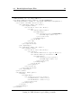
4.1.4
Identity Elements
The Identity class is a default implementation of the Valuation interface in order to
equip NENOK with identity elements. Because of its simplicity and to illustrate
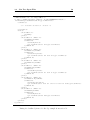
at least once a complete implementation, the code of this class is printed in listing 2. Apart from the methods specified by the Valuation interface or inherited from
java.lang.Object, the Identity class implements further interfaces of the algebraic
framework, namely Scalability and Idempotency. They both extend the Valuation
interface and therefore, we do not necessarily need to enumerate it in the listing
of implemented interfaces. The content of the two new interfaces will be topic of
section 4.2.
4.1.5
Printing Valuation Objects
Naturally, a suitable output format to print valuation objects is a central point but
the way of doing depends greatly on the implemented valuation algebra instance.
Relations and discrete probability distributions (Schneuwly et al., 2004) are typically
represented in table form but we could also imagine the latter as a graphical diagram.
For belief functions (Dempster, 1967; Shafer, 1976) there are perhaps two textual
representations to be considered, once the complete mass function and additionally
only its focal sets. These varying requirements show that we can neither specify the
number nor the signature of output methods in the Valuation interface. NENOK
encounters this fact by introducing a naming convention for such output methods
as follows:
1. Output methods have empty parameter lists and their name is prefixed with
display.
2. Two possible return types are accepted for output methods: java.lang.String
for pure textual output and javax.swing.JComponent for an arbitrary graphical
output component.
4.1
Valuation Algebra Core Components
public f i n a l c l a s s Identity implements Scalability , Idempotency {
public Domain label ( ) {
return new Domain ( ) ;
}
public Valuation combine ( f i n a l Valuation val ) {
return ( Valuation ) val . clone ( ) ;
}
public Valuation marginalize ( Domain dom ) throws VAException {
i f ( dom . size ( ) == 0 )
return new Identity ( ) ;
throw new VAException ( ” I l l e g a l M a r g i n a l i z a t i o n . ” ) ;
}
public i n t weight ( ) {
return 0 ;
}
public String toString ( ) {
return ” I d e n t i t y Element ” ;
}
public boolean equals ( Object o ) {
return ( o instanceof Identity ) ;
}
public Object clone ( ) {
return new Identity ( ) ;
}
public Scalability scale ( ) {
return new Identity ( ) ;
}
}
public Regularity inverse ( ) {
return new Identity ( ) ;
}
Listing 2: Implementation of the Identity class.
17
4.2
Extended Valuation Algebra Framework
18
Software projects that should be able to display valuation objects in a generic way
can invoke these methods by use of the Java Reflection framework (see section 10).
Thereto, NENOK provides a static utility class named Utilities.java that simplifies
this task considerably. We refer to the NENOK Javadoc for more information about
its use. This reflection technique has already been applied convincingly in other
frameworks such as JUnit for example.
4.2
Extended Valuation Algebra Framework
Valuation algebras can have further important properties that are exploited by more
efficient architectures of local computation (Kohlas, 2003). Others are used in order
to optimize the communication costs caused by transmitting valuation objects over
the network (Pouly & Kohlas, 2005). Realizing these properties upon the framework
discussed so far is a big challenge. We must reflect the mathematical relationships
between properties and allow to furnish valuation algebra instances with every mathematically reasonable combination of them. The current NENOK release supports
regular, idempotent, scalable and weight predictable valuation algebras. Figure 4.2
shows how the Valuation interface is accordingly refined.
interface
Valuation
interface
Regularity
interface
Scalability
interface
Idempotency
interface
Predictability
1
Identity
interface
Predictor
Figure 4.2: The extended valuation algebra framework.
4.2.1
Valuation Algebras with Division
Division in the context of valuation algebras is represented by either separative or
regular valuation algebras (Kohlas, 2003). The more general separative algebras
define the division operator across a generic group embedding. This kind of division
is not yet realized in NENOK but only its special case of regular valuation algebras.
4.2
Extended Valuation Algebra Framework
19
The corresponding interface Regularity extends the Valuation interface by adding an
operation to compute inverse valuations. This is how division is implemented in
NENOK. The source of the Regularity interface is given in listing 3.
public i n t e r f a c e Regularity extends Valuation {
public Regularity inverse ( ) ;
}
Listing 3: Listing of the Regularity interface.
We know from (Schneuwly et al., 2004) that an identity element can be adjoined
to regular valuation algebras. Therefore, as already shown in listing 2, the Identity
class needs to implement this interface by itself.
4.2.2
Scalable Valuation Algebras
(Kohlas, 2003) remarks that the existence of scaled valuations depends mainly on
semantic reasons. However, it presumes the division operator and its realization
should therefore extend the Regularity interface. This is shown in figure 4.2. Because the scaling operation is essentially a simple application of division, it could
have been realized by an abstract class that implements Regularity and offers a preimplementation of scaling. The abandonment of this design has very technical but
nevertheless important reasons. It is known that Java does not support multiple
inheritance. If Scalability had been implemented as an abstract class, we would
implicitly hazard the consequences that a scalable instance cannot extend any other
class. We will see that there are other properties that allow to pre-implement some
operators and therefore we will meet this problem again (see section 4.2.3 for example).
There exists in effect a lot of design concepts to avoid multiple inheritance in
Java. In the case at hand, we plumped for an approach called delegation (Gamma
et al., 1993) that is very common to replace inheritance relationships. Basically, we
equip every such interface with an inner class uniformly named Implementor. This
class has an empty constructor and offers methods that correspond to those for
which we want to provide a pre-implementation. In general, these methods take the
current object as additional argument. Listing 4 shows the source of the Scalability
interface together with its inner Implementor class.
A possible instance that wants to use a certain method pre-implementation only
creates an object of its implementor class and calls the corresponding delegator
method. Multiple inheritance is circumvented due to the fact that Implementor is not
coupled with the algebraic framework. If any doubt still lurks in your mind, the
following code snippet shows how to call the scaling delegator:
4.2
Extended Valuation Algebra Framework
20
public Scalability scale ( ) {
return new Scalability . Implementor ( ) . scale ( t h i s ) ;
}
Because an identity element is adjoined to any valuation algebra, the appropriate
Identity class clearly needs to implement the Scalability interface. However, the
implementation of the scale method is trivial in this special case such that the call
of the delegator method becomes unnecessary.
public i n t e r f a c e Scalability extends Regularity {
public Scalability scale ( ) ;
public c l a s s Implementor {
}
public Scalability scale ( Scalability scaler ) {
Scalability v = ( Scalability ) scaler . marginalize (new Domain ( ) ) ;
v = ( Scalability ) v . inverse ( ) ;
return ( Scalability ) scaler . combine ( v ) ;
}
}
Listing 4: Listing of the Scalability interface.
4.2.3
Idempotent Valuation Algebras
Idempotency is a property that applies to the combination operator. We know from
(Kohlas, 2003) that every idempotent valuation algebra is also regular. Therefore,
the corresponding marker interface named Idempotency extends the Regularity interface. Furthermore, we know that in the case of idempotent valuation algebras,
the inverse of a factor collapses with the factor itself. In other words, we can preimplement the inverse method of the Regularity interface for idempotent valuation
algebras. According to the discussion above, this has again been realized by a delegator method within the inner implementor class. The source code of the Idempotency
interface is given in listing 5.
4.2.4
Weight Predictable Valuation Algebras
Although the mathematical concept of weight predictable valuation algebras is
rather simple, its realization turned out to be cumbersome due to the conflictive
requirements. We have seen so far that all properties are represented by an appropriate Java type. To be consistent, this should also be the case for weight predictability. The underlying mathematical idea is that we can compute a valuation’s
4.2
Extended Valuation Algebra Framework
21
public i n t e r f a c e Idempotency extends Regularity {
public c l a s s Implementor {
}
public Regularity inverse ( Idempotency factor ) {
return ( Regularity ) factor . clone ( ) ;
}
}
Listing 5: Listing of the Idempotency interface.
weight even before this valuation really exists. In Java terms, this would demand
for a static implementation. But every valuation algebra possesses its own weight
predictor which contradicts the design based on a static method because they are
shared by all sub-classes and cannot be overwritten. This very short brain storming
shall give an impression of this task’s complexity. In order to meet the requirements
for the most part, we chose to apply again the delegator technique. In NENOK,
weight predictable valuation algebras are mirrored by the Predictability interface
whose source is printed in listing 6.
public i n t e r f a c e Predictability extends Valuation {
public Predictor predictor ( ) ;
}
Listing 6: Listing of the Predictability interface.
The key idea of its only method is to look for the weight predictor of the current
valuation algebra, which is represented by the returned Predictor object. As we can
extract from listing 7 this object computes a valuation’s weight based on its domain.
The design’s only drawback is that we must dispose of at least one valuation object
in order to ask for the weight predictor. But then, we can compute the weight
of an arbitrary non-existing valuation by use of the Predictor. Additionally, we
recommend to all trained Java programmers to implement the Predictor interface as
a SINGLETON design pattern (Gamma et al., 1993) in order to highlight that only
one such object per valuation algebra needs to exist.
Provided that a valuation algebra is weight predictable, we can give a preimplementation of the generic weight method inherited from the Valuation inter-
4.3
Semiring Valuation Algebra Framework
22
public i n t e r f a c e Predictor extends Serializable {
public i n t predict ( Domain dom ) ;
}
Listing 7: Listing of the Predictor interface.
face. The following code delegates its call towards the predictor and exemplifies
furthermore the use of the Predictor object:
public i n t weight ( ) {
return predictor ( ) . predict ( t h i s . label ( ) ) ;
}
The application of the delegator design strategy may seem to complicate the task
but a closer inspection proves that it is of value. First of all, each valuation algebra
implementation can possess its own weight predictor and all objects of this class are
obliged to use it. Second, we can demand the predictor of an arbitrary object in
order to compute the weight of any other instance of the same class. Finally, weight
predictable valuation algebra are realized by a new type which harmonized with the
implementation of other properties.
Developer Notes
• Delegator methods for default implementations are pooled in so-called
Implementor classes in order to avert multiple inheritance dead ends.
• Redirect the call of the weight method to the Predictor instance when
dealing with weight predictable valuation algebras. We recommend furthermore to implement the latter as a SINGLETON design pattern.
• Predictor objects are also used to estimate the weight of remote valuations and need to be serializable on this account.
4.3
Semiring Valuation Algebra Framework
We know from (Kohlas, 2004) that semiring structures induce valuation algebras.
To make allowance for this alternative way of defining valuation algebra instances,
NENOK provides another set of interfaces and classes that extend the general algebraic framework discussed so far. They allow to set up a valuation algebra instance
in a generic way, given an appropriate implementation of semiring values and operations. This section outlines quickly the build-up of this additional framework part
and explains particularly how the semiring components are related to the general
4.3
Semiring Valuation Algebra Framework
23
framework. It is mainly intended for the sake of completeness and is not needed to
understand subsequent sections.
4.3.1
Finite Variables
In the context of semiring induced valuation algebras, frames of variables are always assumed to be finite. The corresponding interface FiniteVariable extends the
Variable marker interface from section 4.1.1 and adds a single method that returns
the frame of the current variable. The frame itself is represented as an array of type
java.lang.Object such that no restriction on the nature of its values is imposed. All
this is shown in listing 8. Generally, it is advisable to use a standard Java type such
as java.lang.String or java.lang.Integer for this task.
public i n t e r f a c e FiniteVariable extends Variable {
public Object [ ] getFrame ( ) ;
}
Listing 8: Listing of the FiniteVariable interface.
Developer Notes
• Make sure that your frame elements are serializable because
FiniteVariable implicitly extends the Serializable interface. Furthermore, they should provide a reasonable equality check and string conversion.
4.3.2
Semiring Elements
The second important component needed to derive a valuation algebra is the implementation of semiring elements. For this purpose, NENOK provides the Element
interface that contains the signature of the two standard semiring operations as
shown in listing 9:
• public Element add(Element e);
The addition of two semiring elements returns a new instance. Thereby, we
meet a similar situation as already discussed in section 4.1.3. Due to the
semiring axioms, addition is associative and commutative. To guarantee these
properties on implementation level, the user must assure that neither of the
involved factors is modified during the computation.
• public Element multiply(Element e);
Multiplication of semiring values also returns a new instances. Because (Kohlas,
4.3
Semiring Valuation Algebra Framework
24
2004) demands commutative semirings for the generic induction of valuation
algebras, we need to ensure associativity and commutativity for this operator. We should again pay attention that no factor is ever modified during the
execution of this operation.
public i n t e r f a c e Element extends Serializable {
public Element add ( Element e ) ;
public Element multiply ( Element e ) ;
}
Listing 9: Listing of the Element interface.
Apart from these typical semiring operations, we need again to adapt methods
inherited from java.lang.Object, namely public boolean equals(Object o) for an equality
check of semiring values and public String toString() for a suitable output format.
Developer Notes
• The resulting element of both addition and multiplication needs to be a
new instance whose memory address differs from the arguments’.
• As every other framework component, the Element implementation must
be fully serializable.
• Overwrite equals and toString from java.lang.Object with an equality
check for semiring elements and a suitable output format respectively.
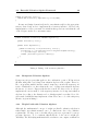
4.3.3
Semiring Valuations
A corresponding user implementation of the two interfaces FiniteVariable and Element
is sufficient for a generic production of a semiring valuation algebra instance. In accordance to the theory developped in (Kohlas, 2004), the class SRValuation generates
all configurations from a given array of finite variables and assigns semiring values
to every configuration. As expected, the class itself implements the Valuation interface from section 4.1.3 and defines the corresponding methods by reducing them to
semiring operations. Among other things, this is illustrated in the class diagram of
figure 4.3.
The default constructor of the class SRValuation mirrors the two semiring related
components. Essentially, this constructor builds the standard enumeration of configurations from an array of finite variables and assigns a semiring element to every
configuration with respect to their ordering. To do so, we must clearly ensure that
4.3
Semiring Valuation Algebra Framework
25
the size of the semiring element array matches with the number of configurations.
If this is not the case, an IllegalArgumentException is thrown.
public SRValuation ( FiniteVariable [ ] vars , Element [ ] values ) ;
Although there is no need for a user extension of the SRValuation class, there
are often good reasons for this voluntary step. Typically, if we want to equip the
implementation with additional constructors or further functionality for example. In
that case, it is indispensable that the extending class provides an empty argument
constructor which will be called by the algebraic framework to ensure correct object
typing. This empty constructor shall simply call the corresponding super constructor
in SRValuation. The reasons are very technical. If a Java class does not possess
any constructor, an implicit empty constructor is added at compile time that calls
its super version. But if a non-empty user defined constructor exists, this must
explicitely be done by the programmer. In NENOK, an UnsupportedOperationException
is thrown when no empty constructor is defined for classes that extend SRValuation.
interface
Valuation
interface
Element
interface
RegularElement
n
n
SRValuation
Configuration
RegularSRValuation
interface
Regularity
ScaledSRValuation
interface
Scalability
Figure 4.3: Semiring framework extension.
Developer Notes
• A correct extension of SRValuation provides an empty constructor that
calls its super constructor.
4.3.4
Regular Semiring Valuations & Scaling
(Kohlas, 2004) states that a positive and regular semiring induces a regular valuation
algebra. In NENOK, elements of such semirings are represented by the RegularElement
interface that extends Element as shown in listing 10 as well as figure 4.3. Thereby,
4.3
Semiring Valuation Algebra Framework
26
the only new method computes the current element’s inverse. We should again be
eager that the implementation of this method demands to return a new class instance
and that no existing object is modified by its call.
public i n t e r f a c e RegularElement extends Element {
public RegularElement inverse ( ) ;
}
Listing 10: Listing of the RegularElement interface.
Accordingly, the class RegularSRValuation extends SRValuation and implements the
Regularity interface in order to produce a regular valuation algebra from an array
of regular and positive semiring elements. Naturally, the corresponding constructor
has the following signature:
public RegularSRValuation ( FiniteVariable [ ] vars , RegularElement [ ] values ) ;
At last, scalable semiring valued valuation algebras are obtained by a simple
extension of RegularSRValuation to ScaledSRValuation which implements furthermore
the Scalability interface. This is due to the fact that scaling does not demand
any additional properties on regular valuation algebras. Moreover, we mentioned
in section 4.2.2 that there are rather semantic reasons for the presence of a scaling
operator, which in case can simply be defined by use of the appropriate implementor.
Developer Notes
• The inverse of a semiring element needs to be a new instance with different memory address.
• A correct extension of both RegularSRValuation and ScaledSRValuation provides an empty constructor that calls its super constructor.
This closes the discussion of the algebraic layer in NENOK. We are aware to
the fact that some design decisions presented here may sill be very elusive. For this
reason, we recommend to dare to tackle your own implementation of a valuation
algebra instance — most of the concepts will quickly become comprehensible. The
next section is dedicated to such an implementation of the standard valuation algebra
framework with the focus on its later usability. This example will attend our studies
through the remaining chapters of this paper and illustrate the future introduced
concepts whenever possible.
5 Case Study: Probability Potentials
5
27
Case Study: Probability Potentials
Probability potentials, extensively described in (Schneuwly et al., 2004), represent
discrete probability distributions which fulfill the axioms of a valuation algebra.
They are well suited to describe the instantiation process of NENOK, because the
valuation algebra operations degrade to simple arithmetic operations. Furthermore,
probability potentials are regular and normalized distributions are obtained by scaling.
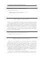
As every NENOK instance, the probability potential implementation is made up
of two classes PP_Variable and Potential respectively. Figure 5.1 shows how these
two components are related to the valuation algebra framework, discussed in the
foregoing section. Note that the shadowed components are part of the algebraic
framework discussed in section 4.
interface
Scalability
Potential
interface
Variable
*
PP_Variable
Figure 5.1: Connecting the probability potential implementation to NENOK.
The implementation of the Variable interface is straightforward and almost selfexplanatory. Its two-argument constructor asks for the variable’s name and its frame,
which is limited to string values as shown below. Both, hash code and equality check
are applied to the variable’s name.
public PP_Variable ( String name , String [ ] frame ) ;
A little more complicated is the implementation of the Valuation interface. We
decided to represent probability potentials internally as an ordered variable array
together with a probability value for each configuration. The advantage of this representation is obvious. We do not need to store all configurations of the potential
explicitly. Clearly, the dimension of the probability array must match the number
of configurations that is given by multiplying the frame cardinality of each variable. Variables and probability values are therefore also the arguments of the class
constructors:
public Potential ( PP_Variable var , double [ ] probs ) ;
public Potential ( PP_Variable var , PP_Variable [ ] cond , double [ ] probs ) ;
The first constructor accepts a single variable with a probability distribution over
its frame values. The second allows additionally to define potentials that are conditioned to an array of variables. Passing an empty variable array to the second
5.1
Probability Potentials in Action
28
constructor amounts to the call of the first one. The remaining work consists of
implementing the framework methods which reduces basically to the manipulation
of the internal probability array. However, we do not go into the details of this
implementation but we will rather take a look at how to model a typical example
using our implementation.
5.1
Probability Potentials in Action
We will use a typical example from bayesian theory, which has been published as a
tutorial for modelling bayesian networks (Charniak, 1991) and is partially inspired
by Pearl’s earthquake example (Pearl, 1988).
I go home at night and I want to know if my family is home before
I try the doors. Often when my wife leaves the house, she turns on
an outdoor light. However, she sometimes turns on this light when she
expects a guest. Also, we have a dog. When nobody is home, the dog is
put in the backyard. The same is true if the dog has bowel troubles. If the
dog is in the backyard, I will probably hear her barking. But sometimes
I can be confused by other dogs barking.
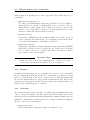
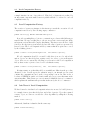
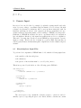
Figure 5.2 shows the causal network that reflects the variables and their relationships within this short tale. Furthermore, it contains a probability distribution for
each identified variable, which are taken from (Charniak, 1991). We will now model
these probability distributions by dint of the probability potential implementation
of the NENOK framework. Thereby, the first step consists in defining the binary
variables.
// There a r e o n l y b i n a r y v a r i a b l e s :
String [ ] frame = { ” 0 ” , ” 1 ” } ;
// The f a m i l y i s o u t :
PP_Variable f = new PP_Variable ( ”F” ,
// Dog has bowel −problem : :
PP_Variable b = new PP_Variable ( ”B” ,
// The l i g h t s a r e on :
PP_Variable l = new PP_Variable ( ”L” ,
// The dog i s o u t :
PP_Variable d = new PP_Variable ( ”D” ,
// Hear b a r k i n g :
PP_Variable h = new PP_Variable ( ”H” ,
frame ) ;
frame ) ;
frame ) ;
frame ) ;
frame ) ;
Next, we define the potentials representing the probability distributions given in
figure 5.2. Note, that we use both constructors and that the potentials are collected
within a common array.
double [ ] probs1 = new double [ ] { 0 . 8 5 , 0 . 1 5 } ;
Potential pot1 = new Potential ( f , probs1 ) ;
5.1
Probability Potentials in Action
29
P(F) = 0.15
P(B) = 0.01
Family out
F
Bowel-Problem
B
Light on
L
Dog out
D
P(D | F B) = 0.99
P(D | F ¬B) = 0.9
P(D | ¬F B) = 0.97
P(D | ¬F ¬B) = 0.3
P(L | F) = 0.6
P(L | ¬F) = 0.05
Hear bark
H
P(H | D) = 0.7
P(H | ¬D) = 0.01
Figure 5.2: Causal network of the dog example.
double [ ] probs2 = new double [ ] { 0 . 9 9 , 0 . 0 1 } ;
Potential pot2 = new Potential ( b , probs2 ) ;
PP_Variable [ ] cond1 = new PP_Variable [ ] {f } ;
double [ ] probs3 = new double [ ] { 0 . 9 5 , 0 . 4 , 0 . 0 5 , 0 . 6 } ;
Potential pot3 = new Potential ( l , cond1 , probs3 ) ;
PP_Variable [ ] cond2 = new PP_Variable [ ] {f , b } ;
double [ ] probs4 = new double [ ] { 0 . 7 , 0 . 0 3 , 0 . 1 , 0 . 0 1 , 0 . 3 , 0 . 9 7 , 0 . 9 , 0 . 9 9 } ;
Potential pot4 = new Potential ( d , cond2 , probs4 ) ;
PP_Variable [ ] cond3 = new PP_Variable [ ] {d } ;
double [ ] probs5 = new double [ ] { 0 . 9 9 , 0 . 3 , 0 . 0 1 , 0 . 7 } ;
Potential pot5 = new Potential ( h , cond3 , probs5 ) ;
Potential [ ] potentials = new Potential [ ] { pot1 , pot2 , pot3 , pot4 , pot5 } ;
Our model delivered a knowledgebase with five potentials. To conclude this
section, we will give a first impression on how to use the valuation algebra framework
by performing some simple computations. To be more concrete, we will solve naively
the projection problem that asks for the dog’s whereabout. Formally:
(φ1 ⊗ φ2 ⊗ φ3 ⊗ φ4 ⊗ φ5 )↓{D} .
This could be done in NENOK by the following lines of code:
Valuation result = new Identity ( ) ;
(5.1)
6 Remote Computing
30
f o r ( Valuation v : potentials ) {
result = result . combine ( v ) ;
}
Domain dom = new Domain (new Variable [ ] {d } ) ;
result = result . marginalize ( dom ) ;
System . out . println ( result ) ;
The computation’s result, printed by the last code line, confirms that the dog is
more likely inside than in the backyard:
−−−−−−−−−−−−−−−−−
|D
| Prob .
|
−−−−−−−−−−−−−−−−−
|0
|0.60
|
|1
|0.40
|
−−−−−−−−−−−−−−−−−
These finger exercises shall give a first picture of how to deal with valuation algebra operations. The next section discusses the remote computing layer of NENOK
and shows how to deal with valuation objects that reside on remote computers. Consequently, it will close by repeating the computation of formula 5.1 but this time
based on distributed probability potentials.
6
Remote Computing
(Pouly & Kohlas, 2005) examined local computation on distributed knowledgebases
and identified processor networks as the central concept for their considerations.
Thereby, processors are defined as independent computing units with their own
memory space such that they can execute tasks without interactions and in parallel.
NENOK adopted this fundamental idea of processors hosting valuation objects and
realized them as ordinary Java threads based on the underlying Jini communication
layer (see figure 3.1). Thus, we can build arbitrary processor networks by starting
processor instances anywhere in the network, or alternatively, we can simulate such
a computing environment on a single machine. The following section shall give the
needed background to set up such a processor network and shows how valuations
spread over such networks can be processed. With respect to figure 3.1 this describes
the NENOK remote computing layer.
6.1
Processor Networks
Each NENOK processor provides some sort of public memory space. It is comparable
to the famous JavaSpace service that is itself based on the Jini framework and offers
a shared virtual object space. However, as we will see, NENOK processors are
more powerful in the sense that they represent real computing units. On the other
hand, NENOK processor can only store Valuation objects and do not provide any
6.1
Processor Networks
31
transaction management. Furthermore, the two distinguish also in the way how
objects in the public space are addressed. But later more about this. For the moment
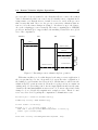
we consider processors exclusively as public valuation storages as illustrated in figure
6.1. Therein, three clients publish valuation objects into the memory space of two
NENOK processors which consist basically of an active storage manager realized as
a Jini service and a memory space (cloud).
Processor 1
φ1
Processor 2
φ3 φ4
φ5
φ2
{φ1 , φ2 }
{φ3 }
{φ4 , φ5 }
Client 1
Client 2
Client 3
Figure 6.1: Publishing valuation objects in a processor’s memory space.
The utility class Services provides a bundle of static methods that are all related
to service administration. Among them, there is a method to start a new processor
instance on the current machine and returns afterwards a proxy towards this service
as described in section 2:
Processor proc = Services . startProcessor ( ) ;
It is possible to set up a Jini environment, even if the current computer is not
connected to any network but only simulates its presence. In this case, a necessary
condition is that the computer disposes of a host name. If this is not the case, the
service method to start processor instances will throw a UnknownHostException. From
a valid host name and the system time of the current computer, one can produce
identifiers that are globally unique to the network. Such an identifier is also assigned
to every processor instance at start time in order to localize it at a later date. Because
identifiers play an important role in all kind of distributed systems, Jini provides a
class named net.jini.id.Uuid for this task. We can request the identifier of a processor
as follows:
Uuid pid = proc . getPID ( ) ;
Once the identifier of a running processor is known, localizing this processor
becomes a simple task by using the appropriate static method of the service class:
Processor proc = Services . findProcessor ( pid ) ;
6.2
Remote Valuation Objects
32
To conclude this short circumscription of a processor’s lifecycle, we point out
that the service class provides also methods to destroy processor instances. Calling
this method will erase the affected processor’s memory space and finally terminate
its thread. The success of the destroy command is indicated by the returned boolean
value.
boolean success = Services . destroyProcessor ( pid ) ;
6.2
Remote Valuation Objects
The consequential step after starting a NENOK processor is naturally the export
of valuation objects into the shared memory space. The related procedure in the
Processor class acts as follows: first, the valuation object is serialized into a byte
stream and transferred towards the processor’s service object which rebuilds the
valuation object in its memory space and wraps it into an Envelope object. These
wrappers serve for addressing purposes because they equip each valuation object
with a unique identifier. Finally, the service object creates a so-called Locator object
which is returned to the client. As we will see below, locators are used to retrieve the
corresponding valuation object from the processor’s public memory. The following
code starts a processor instance and exports the probability potentials from the
previous section into its memory space:
Processor proc = Services . startProcessor ( ) ;
Locator [ ] locators = new Locator [ potentials . length ] ;
f o r ( i n t i = 0 ; i < potentials . length ; i++) {
locators [ i ] = proc . store ( potentials [ i ] ) ;
}
A decisive role play the Locator objects that are returned by the store command. Essentially, locators are catenations of the processor’s ID and the envelope
identifier that encloses the exported valuation within the processor’s memory space.
Therefore, by use of a locator object, we are able to address unambiguously the
corresponding object in the processor’s storage. Moreover, the needed functionality
to retrieve an exported valuation object is offered directly by the Locator class itself
as illustrated below:
Valuation v = locators [ 0 ] . retreive ( ) ;
Locators are very lightweight components which contain essentially only the two
mentioned identifiers. It is therefore much more efficient to transmit locators instead
of their corresponding valuation objects whose weight tends to increase exponentially
as stated in (Pouly & Kohlas, 2005). Figure 6.2 reviews this chain of storing and
retrieving valuation objects by use of an UML sequence diagram. Concluding, the
above code justifies what we have already mentioned in the section dedicated to the
6.3
Knowledgebase Registry
33
algebraic layer, namely that every component of our valuation algebra implementation needs to be fully serializable.
Client
Locator
Processor
store(Valuation)
create(...)
create:Locator
store:Locator
retrieve()
retrieve(...)
retrieve:Valuation
retrieve:Valuation
Figure 6.2: Storing and retrieving valuation objects.
6.3
Knowledgebase Registry
We have seen in figure 6.1 how clients can publish valuation objects in a shared
memory space of a processor and that stored objects can be retrieved later by use
of the appropriate locator which serves intuitively as a global address card. Now,
imagine the following scenario: The barking dog example from section 5.1 shall
be solved again but this time with potentials that are distributed over multiple
processors and no longer local to the computing client. Clearly, we can read valuation
objects from their storing processors as soon as we dispose of the corresponding
locators. The raising question is naturally, how clients can acquire locator objects
that refer to valuations stored by other clients. In other words, we need a way to
exchange locator objects between NENOK clients. This is provided by an additional
Jini service called knowledgebase registry which realizes basically the mathematical
idea of distributed knowledgebases as introduced in (Pouly & Kohlas, 2005). It is
a global service that maps knowledgebase names onto sets of locator objects that
point themselves to remote valuation objects. In figure 6.3 we re-enact the thought
of executing the barking dog example with remote data. Thereby, the five potentials
are distributed over three clients. Each client has already stored its valuations on a
processor and disposes now of the corresponding locators li . Next, they contact the
global registry service and register their locator objects in a common knowledgebase
which can afterwards be downloaded by the computing client.
Let us examine these steps in detail. Each NENOK client can contact the global
knowledgebase registry by use of a static utility method in the service class.
6.3
Knowledgebase Registry
Name
Knowledgebase
"Barking Dog"
{l1 , l2 , l3 , l4 , l5 }
34
{l1 , l2 , l3 , l4 , l5 }
Computing Client
{l1 , l2 }
{l3 }
{l4 , l5 }
Client 1
Client 2
Client 3
Figure 6.3: Clients register their published valuations in a common knowledgebase.
Registry registry = Services . findRegistry ( ) ;
The returned Registry object is again a Jini proxy that allows to communicate
back with the real service running anywhere on the network. This service proxy
allows among other things to create, delete or reset knowledgebases and to add
locator objects to a specific knowledgebase. Finally, each client can download complete knowledgebases from the registry service and knows afterwards the domicile
of each valuation that has been registered within this knowledgebase. Instead of a
complete API discussion, we shall better give a concrete code cutout that illustrates
the communication between NENOK clients and the knowledgebase registry service.
Essentially, the following code performs the activity of client 1 in figure 6.3 by use
of the potentials defined in section 5.1.
Registry registry = Services . findRegistry ( ) ;
registry . createKnowledgebase ( ” Barking Dog” ) ;
Processor proc = Services . startProcessor ( ) ;
Locator loc1 = proc . store ( potentials [ 0 ] ) ;
Locator loc2 = proc . store ( potentials [ 1 ] ) ;
registry . add ( ” Barking Dog” , loc1 ) ;
registry . add ( ” Barking Dog” , loc2 ) ;
Similar steps are accomplished simultaneously by client 2 and 3. Then, the
computing client can download the knowledgebase and retrieve all valuations by
use of the locators in the knowledgebase. It disposes now of an array of potentials
identically to section 5.1 upon which the projection problem could be solved.
Registry registry = Services . findRegistry ( ) ;
Knowledgebase kb = registry . getKnowledgebase ( ” Barking Dog” ) ;
i n t size = kb . size ( ) ;
Valuation [ ] vals = new Valuation [ size ] ;
6.4
Remote Valuation Algebra Operations
35
f o r ( Locator loc : kb ) {
vals [ size −1] = loc . retrieve ( ) ;
size −−;
}
A component that shall be surveyed in more detail is the Knowledgebase class.
We have already mentioned that these objects represent the mathematical idea of
a distributed knowledgebase, i.e. a collection of remote valuations together with a
mapping that tells us on which processors they reside. Clearly, a set of locators fulfils
this definition. Although a knowledgebase is internally just a simple Java set type
that includes locator objects, there are nevertheless some important issues to bring
up. A knowledgebase affiliates only valuations of the same type (ignoring identity
elements). It is therefore impossible to mix valuation objects of different algebra
instances in the same knowledgebase. However, because locators are only pointers
to remote valuations, this type-checking cannot be done at compile time. So, the first
inserted element determines the type that is accepted by a certain knowledgebase
and an IllegalArgumentException is thrown when this policy is violated at a particular
time. Concluding, we remark once more that shipping a knowledgebase over the
network is comparatively cheap because they consist only of lightweight locator
objects.
6.4
Remote Valuation Algebra Operations
Regarding the foregoing code snippet, we observe that once the knowledgebase is
downloaded, every valuation is fetched by the client in order to fill the valuation
array that is needed to carry out the computations. This causes unnecessary communication costs, especially when we are not interested in the factor array by itself
but only in the final result of the computations. NENOK provides a solution for
this worry by executing the basic valuation algebra operations remotely, i.e. directly
on the processor that hosts the involved factors. This possibility has already been
foreshadowed in section 6.1 as we introduced processors as independent computing
units rather than just dumb memory guards. This ability is based on a distributed
version of the COMMAND design pattern (Gamma et al., 1993). The characteristic
idea is to encapsulate a valuation algebra operation together with its factors into an
object which can be transmitted afterwards to the processor that is assigned with
its execution. As a matter of course, we do not wrap valuation objects into these
command object but only the locators pointing to the corresponding valuations.
The processor’s execution method has the following signature:
public Locator execute ( Task task ) throws RemoteException , VAException ;
Task constitutes the head interface of the COMMAND design pattern and defines
accordingly the signature of a no-argument execution method that will be called by
the processor. Furthermore, it clearly extends for good reasons the Serializable
interface. For every basic valuation algebra operation, there is a class that extends
6.4
Remote Valuation Algebra Operations
36
the Task interface and performs the operation according to its name. This is shown
in class diagram 6.4.
interface
Serializable
interface
Task
Combination
Marginalization
Inverse
Figure 6.4: The class diagram of the distributed COMMAND pattern.
The above execution method of the processor returns a Locator object that points
to the computation’s result. By convention, the result of each computation is stored
in the public memory of the computing processor itself which is therefore capable
to create and return an appropriate locator. Doing so, we prevent once more unnecessary costs. The detailed communication chain of executing a remote operation
is illustrated in the sequence diagram of figure 6.5. More precisely, the first step
consists in creating a Task object for the valuation algebra operation to execute.
This is done via a factory method in a class named TaskFactory. The mission of this
class is exactly what its name leads one to assume. It provides methods to create Task objects for all basic valuation algebra operations, i.e. it instantiates every
class implementing the Task interface. The reasons for this redirection are manyfold,
thereunder the possibility to count operations during local computation. But this
will be topic of another chapter. In a nutshell, the factory’s creator methods are:
• public static Task createCombination(Locator factor1, Locator factor2);
Creates a task to compute the combination of two valuations that are referenced by the locators given as argument.
• public static Task createMarginalization(Locator factor, Domain dom);
Creates a task to compute the marginalization of a valuation, referenced by
the locator, to the given domain.
• public static Task createInverse(Locator factor);
Creates a task to compute the inverse of a valuation referenced by the locator.
Once such a task object is created, a hand-picked processor is contacted in order
to make it execute the task. As shown in figure 6.5, the processor carries out the
task locally and wraps the resulting valuation into an envelope (i.e. equips it with
an identifier). Thereafter, this envelope is stored in the public memory space of the
6.4
Remote Valuation Algebra Operations
37
processor and a locator is returned to the client that allows to retrieve the result if
desired. Alternatively, this locator can be used for further remote computations. It
is important to note that the factors of a task do not need to reside on the processor
that executes this task. Moreover, the processor can retrieve valuations that are
remote to it by the same technique as clients do. It is therefore up to the client to
choose the computing processor reasonably. The remote computing layer of NENOK
provides no internal logic to support this decision making because there is no global
view of the computation.
TaskFactory
Client
Task
Processor
create
create:Task
execute(Task)
execute
execute:Evelope
store(Envelope)
store:Locator
execute:Locator
Figure 6.5: Executing a remote valuation algebra operation.
With a fine tradition, we close this chapter by showing a concrete application of
the concepts introduced so far. As promised, we repeat the naive computation of
the barking dog problem introduced in section 5.1 but this time we will execute the
valuation algebra operations remotely. From the foregoing sections, we assume an
existing array of locators that point to the five input valuations and reuse the same
domain for the final marginalization as in section 5.1. To stress a short and clearly
arranged code, we delegate all computations to a single processor. This is of course
not a very clever choice regarding the computation’s communication costs.
Processor proc = Services . startProcessor ( ) ;
TaskFactory factory = new TaskFactory ( ) ;
Locator result = locators [ 0 ] ;
f o r ( i n t i = 1 ; i < locators . length ; i++) {
Task task = factory . createCombination ( result , locators [ i ] ) ;
result = proc . execute ( task ) ;
}
Task task = factory . createMarginalization ( result , dom )
7 Running a NENOK Federation
38
result = proc . execute ( task ) ;
System . out . println ( result . retrieve ( ) ) ;
As shown below, the results are equal, independent of their local or remote
execution. We would furthermore remind that the temporary results obtained from
the combination task remain in the processor’s public memory and therefore are
never shipped until we explicitly ask for in the last statement.
−−−−−−−−−−−−−−−−−
|D
| Prob .
|
−−−−−−−−−−−−−−−−−
|0
|0.60
|
|1
|0.40
|
−−−−−−−−−−−−−−−−−
We mentioned already that the TaskFactory object does not only create new tasks
but also serves as a statistician within our framework. We illustrate this by asking
the number of created combination tasks. The given answer will be 4.
System . out . println ( factory . getCombinations ( ) ) ;
The next section is dedicated to the setup of a running NENOK federation such
that the reader can start its own experimenting. Particularly, we will discuss an
important point that has been omitted in the last section, namely how to start a
registry service.
7
Running a NENOK Federation
Setting up a Jini environment is known to exasperate users due to the endless configuration work. A major attend in the development of NENOK was to prevent
the user as much as possible from this arduousness by offering pre-configured start
procedures for all related Jini services. This section should lead the user towards a
running NENOK federation. To do so, we will show how the underlying Jini environment with two support services is set up and complete the federation afterwards
by launching a central knowledgebase registry service. Closing, we will also describe
the measures to take in order to run the programs of the former sections.
In section 2 we learned about the importance of so-called support services in
every Jini system and two of them constitute NENOK’s underlying Jini environment, namely a HTTP server and Reggie. Because Reggie by itself is a Jini service
and depends on a running HTTP server, the order to start the Jini environment
components is strictly predetermined. To simplify the user’s life, NENOK delivers
all necessary start scripts for both systems (bat and sh-scripts) in its startup folder.
Nevertheless, some minor configuration work is indispensable and described below
by example of the Windows start scripts.
7.1
HTTP Server
7.1
HTTP Server
39
The standard Jini distribution contains already a simple HTTP server implementation which is by far sufficient for our purposes. The corresponding script named
classserver.bat launches the server as follows:
java −Djava . security . policy=policy . all ˆ
−Dport =8081 ˆ
−jar . . \ jini \ start . jar ˆ
start−classserver . config
pause
Because NENOK comes in a standalone distribution and contains all Jini archives
by itself, a lot of configuration work is therefore put aside by using relative paths. A
very important point is the specification of the NENOK port which is by default set
to 8081. We recommend to not modify it unless another application on your system
already use this port.
7.2
Reggie
Reggie is the default implementation of a lookup service and composes the second
bridge pier of the Jini environment. Because Reggie is a real Jini service by itself, it
must know the address of the HTTP server that hosts its reconstruction code (see
section 2.2). This has been denoted as codebase and should point to the currently
started HTTP server. Modify the following script named reggie.bat in such a way
that the IP address corresponds to the machine running the HTTP server. If you
changed the port number in the webserver’s start script, the corresponding value
must also be adapted.
java −Djava . security . policy=policy . all ˆ
−Dcodebase=http : / / 1 3 4 . 2 1 . 7 3 . 9 1 : 8 0 8 1 / ˆ
−jar . . \ jini \ start . jar ˆ
start−transient−reggie . config
pause
7.3
Knowledgebase Registry
Once the Jini environment is running, we can finally run the knowledgebase registry
by use of the script registry.bat. Comparably to Reggie, this service is global to
the NENOK federation and therefore started manually. Again, we need to ensure
that the codebase refers to the running HTTP server such that it can download the
reconstruction code. The same remark applies to the port number.
java −cp . . \ jini \ reggie . jar ˆ
−Djava . security . policy=policy . all ˆ
−Dcodebase=http : / / 1 3 4 . 2 1 . 7 3 . 9 1 : 8 0 8 1 / ˆ
−jar . . \ jini \ start . jar ˆ
7.4
Starting a NENOK application
40
start−transient−registry . config
pause
All services discussed so far use a policy file named policy.all that grants all
privileges to the appropriate service. Although this policy is not recommended in a
commercial system, the configuration of a secure Jini system goes beyond the scope
of this paper.
7.4
Starting a NENOK application
A running HTTP server together with Reggie and a knowledgebase registry constitutes a complete NENOK environment in which the remote computing application
of section 6.4 can be started. Assume therefore a compiled file Dog.class that contains this code completed and packed in a main method. Note that you need to add
the files nenok.jar and ppotentials.jar to the classpath for compilation. Running
this application is a bit more tricky because we start a processor instance that is
a Jini service. Apart from the classpath, we must therefore again pay attention to
the correct setting of the codebase that includes this time the reconstruction code
of the processor implementation and also the probability potential implementation.
java −cp ” . ; . . \ p p o t e n t i a l s . j a r ; . . \ . . \ l i b \ nenok . j a r ” ˆ
−Djava . rmi . server . codebase= ˆ
” h t t p : / / 1 3 4 . 2 1 . 7 3 . 9 1 : 8 0 8 1 / l i b / p r o c e s s o r −d l . j a r ˆ
http : / / 1 3 4 . 2 1 . 7 3 . 9 1 : 8 0 8 1 / p p o t e n t i a l s 1 .1/ p p o t e n t i a l s . j a r ” ˆ
−Djava . security . policy = . . \ . . \ policy . all Dog
pause
By the way, this illustrates best the power and flexibility of a Jini service. Assume that processor A creates a knowledgebase and loads a collection of locators
up to this knowledgebase. Then, another processor B downloads this knowledgebase and tries to retrieve the probability potential objects from the locators within
that knowledgebase. In order to deserialize the potential objects, processor B must
clearly know their implementation which is not necessarily the case. But due to the
codebase information, processor B can download the appropriate class files from the
HTTP server and use the objects as if they were created locally.
8
Local Computation
We now arrived almost on the crest of the NENOK layer model and describe how
local computation techniques can be applied to any given valuation algebra implementation. Thereby, there are a great many of involved components such as the
various architectures of local computation or join tree construction algorithms that
allow to parameterize NENOK by some means or other. But this multiplicity of
possibilities runs naturally the risk of overstraining users that simply want to perform some basic computations. Therefore, the guiding idea of NENOK is to provide
a fully configured system by default and to allow changing these values by use of
8.1
Local Computation Factory
41
a simple interface in case of special need. This level of abstraction is realized by
an important component named LCFactory which will also be referred to as local
computation factory.
8.1
Local Computation Factory
The creation of a LCFactory instance is the first step towards the execution of local
computation and done by the following empty constructor.
public LCFactory ( ) throws UnknownHostException ;
It provides a multiplicity of join tree construction procedures with different parameter lists. We agree at this place to the two most basic creators and put off the
subsequent sections that will complete this listing. The first creator allows to build
join trees directly from a given knowledgebase and a list of queries, represented by
Domain objects. The local computation factory ensures that these queries are covered
by the resulting join tree.
public JoinTree create ( Knowledgebase kb , List<Domain> queries ) ;
If local computation should be executed locally, there is no need to upload valuation objects on a knowledgebase registry service in order to get a Knowledgebase
object. Moreover, we can use the following second creation of the local computation
factory that creates a join tree based on a local valuation array.
public JoinTree create ( Valuation [ ] vals , List<Domain> queries ) ;
It is important to note that this call does essentially not differ from the procedure
discussed so far. It will export the valuation array to an internal processor and
continue the computations based on the corresponding locators. In other words: a
local use of NENOK is equal to a federation with only one processor that runs on the
current machine. This private processor is started within the factory’s constructor
which explains the UnknownHostException that is thrown by the above constructor.
8.2
Join Trees & Local Computation
We have learned so far that local computation factories are used to build join trees,
for example from a given knowledgebase and a list of queries. Upon the returned
JoinTree object, we can now execute the collect algorithm by calling the following
method:
public void collect ( ) ;
Afterwards, distribute is launched in the same way:
public void distribute ( ) ;
8.3
Architectures of Local Computation
42
Finally, we can answer queries by use of the following method:
public Valuation answer ( Domain query ) throws RemoteException ;
This method looks recursively for a join tree node that covers the given query and
loads the valuation from the processor assigned to this node. As usual, an exception
is thrown in case of communication problems and null is returned if no covering
node for the given query was found. This outlines briefly how NENOK can be
used to perform local computation. It is furthermore remarkable that due to the
default configurations, only five lines of code were needed for this complex task.
Nevertheless, there are many other interesting functionalities provided by NENOK
such as its ability for statistical monitoring. The following methods are all part of
the JoinTree class and can be used to analyze local computation:
• public double getCollectTime();
Measures the time in milliseconds needed by the collect algorithm.
• public double getDistributeTime();
Measures the time in milliseconds needed by the distribute algorithm.
• public int getCommunicationCosts();
Measures the communication costs of local computation.
• public Set<Processor> getProcessorSet();
Returns the set of all processors that are assigned to nodes of this join tree.
In section 6.4 we have seen that remote command objects can only be created
by use of a TaskFactory instance. Every join tree holds its own task factory which is
created in parallel to the join tree itself and from which it gets the needed command
objects for local computation. Therefore, as shown in section 6.4, we can refer to
this object in order to ask for the number of executed operations:
public TaskFactory getTaskFactory ( ) ;
This listing contains only a very small subset of the methods provided by the
class. During the following sections, we will accent some more of them if
their functionality is directly related with the topic under discussion.
JoinTree
8.3
Architectures of Local Computation
We have seen in the foregoing sections how NENOK can be used to perform local
computation, although we have never specified the architecture that was applied.
Now the time has come to eliminate this unknown. But first, we need to have an idea
about the implementation of local computation in NENOK, especially we should be
curious how architectures of local computation are realized.
In NENOK, join trees are implemented traditionally as doubly linked Node objects such that one can traverse them in both directions for collect and distribute
8.3
Architectures of Local Computation
43
respectively. Each node contains therefore only pointers to its neighbors and to
make a long story short, no information about the global state of the tree. This is
furthermore provided by the JoinTree class, which holds a pointer to the root node
together with a multiplicity of global information about the current tree. Hence,
every architecture of local computation is built up from two classes that extend the
Node class as well as the JoinTree class. In short, each architecture for local computation corresponds to a join tree implementation. This is shown in figure 8.1 for
the case of the Shenoy-Shafer architecture. Please note that for better readability,
the class names of the Shenoy-Shafer components do not correspond exactly to their
real-world pendants.
1
JoinTree
Node
Shenoy-Shafer
JoinTree
Shenoy-Shafer
Node
Implementation of the
Shenoy-Shafer Architecture
Figure 8.1: Implementation of the Shenoy-Shafer architecture.
There is another important point to address at this place, although its direct
consequences may not yet be apparent. Each join tree type should know the kind
of Node from which it is built up. As we will see, this is especially important in
the context of join tree construction. For this purpose, the JoinTree class defines
an abstract method that returns a new node object corresponding to the join tree
architecture.
public abstract Node createNode ( ) ;
To be more concrete, in the case of the Shenoy-Shafer join tree this method will produce a new Shenoy-Shafer node instance. We will refer to this important relationship
in section 8.4, but first let us show how easily join trees of different architectures
can be constructed.
In section 8.1 we have seen that join trees are constructed by use of the LCFactory
class. Hence, these objects must antecedently know which kind of join tree to construct and therefore hold an internal field that provides this information. Consequently, the user can switch the architecture just by resetting the corresponding
value in the local computation factory. To make this task even more comfortable,
NENOK provides a Java Enum type named Architecture that contains a pseudoconstant value for each available architecture. To change the architecture value of
the LCFactory class, the following method can now be used.
8.4
Join Tree Construction Algorithms
44
public void setArchitecture ( Architecture architecture ) ;
After this call, the factory will produce join trees corresponding to the architecture
constant given as argument. By default, the architecture value of the local computation factory corresponds to the Shenoy-Shafer architecture. In the current NENOK
version, the user can choose between the following architecture constants:
• Architecture.Shenoy_Shafer
• Architecture.Binary_Shenoy_Shafer
• Architecture.Lauritzen_Spiegelhalter
• Architecture.Hugin
• Architecture.Idempotent_Architecture
To contribute to the listing of informational methods in section 8.2, the architecture of a given join tree can be asked by applying the following method to the
JoinTree object.
public String getArchitecture ( ) ;
We omitted to declare in section 8.1 that the factory’s method collection to
construct join trees may all throw a ConstrException. This is namely the case if the
given knowledgebase to build the covering tree does not respect the mathematical
restrictions imposed on the factory’s current architecture value. Such exceptions are
thrown for example if we try to construct a Lauritzen-Spiegelhalter join tree with
a knowledgebase whose underlying valuation algebra does not define any division
operator.
8.4
Join Tree Construction Algorithms
The complexity of local computation depends mainly of the size of the largest node
domain in the join tree. Therefore, the construction of a suitable join tree is of
prime importance. Unfortunately, we know also that finding the optimum join
tree is an NP-hard problem (Arnborg et al., 1987) which compels us in general to
apply heuristics. This is turn justifies our interest in having multiple, exchangeable
construction algorithms such that we can compare the quality of the constructed
join trees. The JoinTree class provides the following methods to analyze the quality
of a join tree.
• public int countNodes();
Returns the number of nodes in the current join tree.
• public Domain getLargestDomain();
Returns the largest join tree node domain of the current join tree.
8.4
Join Tree Construction Algorithms
45
Additionally, a join tree construction algorithm should be highly independent
to the architecture of the constructed join tree. In other words, each construction
algorithm should be able to construct join trees of arbitrary architectures. Already
the first NENOK version provided a very sophisticated design solution for this task
that has proven its worth. This strategy shall be sketched in this section, again with
the focus on its usability.
Construction algorithms in NENOK are realized by application of the COMMAND design pattern (Gamma et al., 1993). The common abstract head class
named Algorithm contains the following signature:
public abstract Node buildTree ( JoinTree . Construction data ) ;
The return value of this method is the root node of the created join tree and its
only argument is a wrapper defined within the JoinTree class that allows basically to
feed the construction algorithm with arbitrary input data. In addition, the Algorithm
class provides two other informative methods:
• public String getName();
Returns the name of this construction algorithm.
• public double getConstructionTime();
Returns the measured time in milliseconds of the algorithm’s last run.
Most construction algorithms are based on variable elimination. Therefore, a
further abstract class named Elimination exists which refines Algorithm by a new
method that stores the variable elimination sequence during the algorithm’s run:
public Variable [ ] getEliminationSequence ( ) ;
Figure 8.2 summarizes the class dependencies of the construction algorithm
framework part and shows furthermore three pre-implemented algorithms that are
at the user’s disposal:
1. One Step Look Ahead Smallest Clique: This very efficient construction algorithm has been defined in (Lehmann, 2001) and is based on a heuristics that
eliminates variables in a specific order derived from their occurrences in the
knowledgebase. The realizing class is called OSLA_SC and constitutes the default
algorithm of NENOK.
2. Static Sequence: The static sequence algorithm allows to force a formerly defined variable elimination sequence. It is especially useful to study the impact
of a suitable elimination sequence on the tree width, i.e. the size of the largest
join tree node domain. The corresponding class is named Sequence and its
constructor demands a complete variable sequence defining the elimination
order.
8.4
Join Tree Construction Algorithms
46
3. Deserializer : Empiric verification of theoretical results is often only possible
if one can specify the exact shape of a join tree and this is hardly possible
with variable elimination. The Deserializer class allows therefore to specify
the exact buildup of a join tree in an external file and realizes the tree as it
has been described. We only list this method for the sake of completeness and
refer to section 9 that is fully dedicated to this feature.
abstract
Algorithm
abstract
Elimination
Deserializer
OSLA_SC
Sequence
Figure 8.2: Framework part that specifies join tree construction algorithms together
with three pre-implementations.
Changing the default construction algorithm in NENOK is an artless task, thanks
again to the local computation factory. Because this component supervises join
tree construction, we can proceed in the same manner as for changing the local
computation architecture. The only difference is that instead of constant values, we
directly pass an object of the corresponding algorithm to the factory which in turn
will use this algorithm to construct future join trees. The signature of this method
is:
public void setConstructionAlgorithm ( Algorithm algo ) ;
A further advantage of this procedure it that every user can in principle realize its
own join tree construction algorithm by implementing the Algorithm interface. Then,
by use of the foregoing method, this user implementation can be applied carefree
within the local computation factory.
We learned in the foregoing section that each local computation architecture is
made up from two classes extending JoinTree and Node respectively. But on the other
hand, each join tree construction algorithm should be able to build any kind of join
tree, i.e. the construction process should be independent of the tree’s architecture.
This interplay is ruled as follows and illustrated in sequence diagram 8.3. An important role plays thereby the already mentioned method of the JoinTree class that
returns the appropriate node type for each architecture.
8.4
Join Tree Construction Algorithms
47
1. The local computation factory calls the constructor of the JoinTree class that
corresponds to its architecture value with the construction algorithm as argument.
2. The constructor creates a wrapper object named JoinTree.Construction that
contains all needed data to build join trees. Beside knowledgebase and query
list, the constructor links itself into this object which is afterwards passed to
the construction algorithm.
3. Whenever the construction algorithm requires a new Node object to build the
tree, it performs a callback to the JoinTree class via the reference stored in the
wrapper object. Thereby, it calls the createNode() method addressed in section
8.3 and gets a new node instance that corresponds to the current architecture.
Client
LCFactory
create
JoinTree
Algorithm
new JoinTree
buildTree
createNode
createNode:Node
buildTree:Node
create:JoinTree
Figure 8.3: A sequence diagram for the join tree construction process.
Again, we extend the listing of the JoinTree class’ informative methods given in
section 8.2 by the following method that allows to access the construction algorithm
which created the current tree:
public String getArchitecture ( ) ;
Traditionally, we close the discussion on local computation in NENOK by a
concrete application of the concepts introduced in this section. To do so, we will
repeat the computations of section 6.4 but this time by use of local computation
techniques. To start with, we download again the knowledgebase from the registry
service and fill an array with our queries of interest. Then, we need to construct a
local computation factory:
Domain [ ] queries = new Domain [ ] { dom } ;
8.4
Join Tree Construction Algorithms
48
Knowledgebase kb = registry . getKnowledgebase ( ” Barking Dog” ) ;
LCFactory factory = new LCFactory ( ) ;
The first application executes local computation with the factory’s default values,
i.e. a Shenoy-Shafer join tree is built by use of the OSLA-SC construction algorithm:
JoinTree jt1 = factory . create ( kb , Arrays . asList ( dom ) ) ;
jt1 . collect ( ) ;
jt1 . distribute ( ) ;
System . out . println ( jt1 . answer ( dom ) ) ;
Clearly, the printed result is identical to section 6.4:
−−−−−−−−−−−−−−−−−
|D
| Prob .
|
−−−−−−−−−−−−−−−−−
|0
|0.60
|
|1
|0.40
|
−−−−−−−−−−−−−−−−−
Next, we configure the local computation factory in such a way that a static sequence
construction algorithm with a user-defined elimination sequence is used to build the
join tree. Additionally, because probability potentials are regular, we demand the
factory to construct a Hugin join tree:
factory . setArchitecture ( Architecture . HUGIN ) ;
Algorithm algo = new Sequence (new Variable [ ] {f , b , l , d , h } ) ;
factory . setConstructionAlgorithm ( algo ) ;
JoinTree jt2 = factory . create ( kb , Arrays . asList ( dom ) ) ;
jt2 . collect ( ) ;
jt2 . distribute ( ) ;
System . out . println ( jt2 . answer ( dom ) ) ;
Again, the result is:
−−−−−−−−−−−−−−−−−
|D
| Prob .
|
−−−−−−−−−−−−−−−−−
|0
|0.60
|
|1
|0.40
|
−−−−−−−−−−−−−−−−−
At last, we want to convince the reader that the two join trees really differ in their
shape. For this purpose, we ask for the largest node domain in both join trees:
System . out . println ( jt1 . getLargestDomain ( ) ) ;
System . out . println ( jt2 . getLargestDomain ( ) ) ;
It should not be amazing that the OSLA-SC has built a better join tree than our
randomly chosen elimination sequence:
9 Generic Input
49
{D , F , B}
{D , F , B , L}
9
Generic Input
In section 5.1 we modeled the dog example by explicitly creating variable and valuation objects according to our valuation algebra instance. For broader models with
perhaps a few thousand of valuations, this becomes an almost intractable task. In
particuar, such huge models are often output by another program that is not necessarily written in Java which makes a direct binding to NENOK often impossible.
Furthermore, NENOK should incite the user to experiment with local computation
but each slight modification of the input data results in the need for recompilation.
This can be very annoying. For those reasons, NENOK provides a system for generic
input processing. Thereby, the key elements are a generic XML data structure as
well as a parser framework that must again be implemented for the valuation algebra
at hand.
9.1
Knowledgebase Input Files
To perform local computation, NENOK must be fed with the following input data:
• the variables of the knowledgebase,
• the valuations,
• the queries of interest that must be covered by the join tree.
This is incorporated by the skeleton of the following generic XML file:
<k n o w l e d g e b a s e>
<v a r i a b l e s>
<v a r i a b l e varname=”v1 ”>. . .</ v a r i a b l e>
..
.
</ v a r i a b l e s>
<v a l u a t i o n s>
<v a l u a t i o n>. . .</ v a l u a t i o n>
..
.
</ v a l u a t i o n s>
<q u e r i e s>
<query>. . .</ query>
..
.
</ q u e r i e s>
</ k n o w l e d g e b a s e>
The <knowledgebase> tag contains the elements <variables>, <valuations> and voluntarily <queries>, respecting the given order. Inside, all three elements can contain
9.1
Knowledgebase Input Files
50
an arbitrary number of their corresponding sub-tags. The <variable> elements in
particular possess an attribute that denotes the name of the represented variable.
This name must be unique and will be referenced by the content of the <query> tag.
The remaining content together with the content of the <valuation> tags constitute
the generic part of this structure that will be addressed below. More structured is
the inside of the <query> elements that has to be a list of white space separated
variable names. This is a generic structure due to the unspecified content of the
<variable> and <valuation> tags. We refer to listing 11 that models the input data of
the dog example (section 5.1) by use of this skeleton.
To validate such files concretely, NENOK provides an XML Schema file called
va.xsd that defines the buildup of this skeleton formally. Thereby, the inside of
<variable> and <valuation> is specified as follows:
<x s : e l e m e n t name=” v a r i a b l e ” ty pe=” v a r c o n t e n t ” />
<xs:complexType name=” v a r c o n t e n t ”>
< x s : a t t r i b u t e name=” varname ” type=” x s : I D ” u s e=” r e q u i r e d ” />
</ xs:complexType>
<x s : e l e m e n t name=” v a l u a t i o n ” ty pe=” v a l c o n t e n t ” />
<xs:complexType name=” v a l c o n t e n t ” />
va.xsd
NENOK Schemas
As we can see, the Schema prescribes an empty content for <variable> as well as for
<valuation> tags. Thus, this Schema would rightly not validate listing 11. However,
XML Schema provides a feature that allows to include and redefine elements via
<xs:redefine schemaLocation=”...”> and this technique will be used to adapt the global
skeleton Schema to a specific user instance. More precisely, the user creates its own
XML Schema file that redefines the two elements <varcontent> and <valcontent> from
va.xsd. All other elements of the file skeleton are fully specified and do not need
to be redefined. This relationship between XML Schemata is illustrates in figure
9.1. Listing 12 adapts va.xsd to probability potentials such that our input file from
listing 11 validates correctly.
ppotential.xsd
User Schemas
redefines
Figure 9.1: XML Schema relationships: NENOK Schemas vs. User Schemas
9.1
Knowledgebase Input Files
51
<?xml version=” 1 . 0 ” e n c o d i n g=”UTF−8” ?>
<k n o w l e d g e b a s e x m l n s : x s i=” h t t p : //www. w3 . o r g /2001/XMLSchema−i n s t a n c e ”
xsi:noNamespaceSchemaLocation=” p p o t e n t i a l . xsd ”>
<v a r i a b l e s>
<v a r i a b l e varname=”F”>
<frame>0 1</ frame>
</ v a r i a b l e>
<v a r i a b l e varname=”L”>
<frame>0 1</ frame>
</ v a r i a b l e>
<v a r i a b l e varname=”D”>
<frame>0 1</ frame>
</ v a r i a b l e>
<v a r i a b l e varname=”B”>
<frame>0 1</ frame>
</ v a r i a b l e>
<v a r i a b l e varname=”H”>
<frame>0 1</ frame>
</ v a r i a b l e>
</ v a r i a b l e s>
<v a l u a t i o n s>
<v a l u a t i o n>
< l a b e l>F</ l a b e l>
< p r o b a b i l i t i e s>0 . 8 5 0 . 1 5</ p r o b a b i l i t i e s>
</ v a l u a t i o n>
<v a l u a t i o n>
< l a b e l>L F</ l a b e l>
< p r o b a b i l i t i e s>0 . 9 5 0 . 4 0 . 0 5 0 . 6</ p r o b a b i l i t i e s>
</ v a l u a t i o n>
<v a l u a t i o n>
< l a b e l>H D</ l a b e l>
< p r o b a b i l i t i e s>0 . 9 9 0 . 3 0 . 0 1 0 . 7</ p r o b a b i l i t i e s>
</ v a l u a t i o n>
<v a l u a t i o n>
< l a b e l>D F B</ l a b e l>
< p r o b a b i l i t i e s>0 . 7 0 . 0 3 0 . 1 0 . 0 1 0 . 3 0 . 9 7 0 . 9 0 . 9 9</ p r o b a b i l i t i e s>
</ v a l u a t i o n>
<v a l u a t i o n>
< l a b e l>B</ l a b e l>
< p r o b a b i l i t i e s>0 . 9 9 0 . 0 1</ p r o b a b i l i t i e s>
</ v a l u a t i o n>
</ v a l u a t i o n s>
</ k n o w l e d g e b a s e>
Listing 11: Input data of the dog example from section 5.1.
9.1
Knowledgebase Input Files
<?xml version=” 1 . 0 ” e n c o d i n g=”UTF−8” ?>
<x s : s c h e m a x m l n s : x s=” h t t p : //www. w3 . o r g /2001/XMLSchema”
elementFormDefault=” q u a l i f i e d ” a t t r i b u t e F o r m D e f a u l t=” u n q u a l i f i e d ”>
< x s : r e d e f i n e schemaLocation=” va . xsd ”>
<xs:complexType name=” v a r c o n t e n t ”>
<x s : c o m p l e x C o n t e n t>
<x s : e x t e n s i o n b a s e=” v a r c o n t e n t ”>
< x s : a l l>
<x s : e l e m e n t name=” frame ”>
<x s : s i m p l e T y p e>
< x s : r e s t r i c t i o n b a s e=”xs:NMTOKENS”>
<x s :m in L e n gth v a l u e=” 1 ” />
</ x s : r e s t r i c t i o n>
</ x s : s i m p l e T y p e>
</ x s : e l e m e n t>
</ x s : a l l>
</ x s : e x t e n s i o n>
</ x s : c o m p l e x C o n t e n t>
</ xs:complexType>
<xs:complexType name=” v a l c o n t e n t ”>
<x s : c o m p l e x C o n t e n t>
<x s : e x t e n s i o n b a s e=” v a l c o n t e n t ”>
<x s : s e q u e n c e>
<x s : e l e m e n t name=” l a b e l ” ty pe=” dom type ” />
<x s : e l e m e n t name=” p r o b a b i l i t i e s ”>
<x s : s i m p l e T y p e>
< x s : r e s t r i c t i o n b a s e=” p l i s t ”>
<x s :m in L e n gth v a l u e=” 1 ” />
</ x s : r e s t r i c t i o n>
</ x s : s i m p l e T y p e>
</ x s : e l e m e n t>
</ x s : s e q u e n c e>
</ x s : e x t e n s i o n>
</ x s : c o m p l e x C o n t e n t>
</ xs:complexType>
</ x s : r e d e f i n e>
<x s : s i m p l e T y p e name=” p l i s t ”>
< x s : l i s t>
<x s : s i m p l e T y p e>
< x s : r e s t r i c t i o n b a s e=” x s : d o u b l e ”>
<x s : m i n I n c l u s i v e v a l u e=” 0 . 0 ” />
<x s : m a x I n c l u s i v e v a l u e=” 1 . 0 ” />
</ x s : r e s t r i c t i o n>
</ x s : s i m p l e T y p e>
</ x s : l i s t>
</ x s : s i m p l e T y p e>
</ x s : s c h e m a>
Listing 12: XML Schema for probability potentials.
52
9.1
Knowledgebase Input Files
53
The last milestone in the description of generic input processing is the parsing
process itself. From a bird’s eye view, this is shown in figure 9.2. Essentially,
the parser component transforms the input data from a given XML file into an
array of Valuation and an array of Domain objects representing the queries. The two
components are wrapped into a class named ResultSet such that they can both be
returned by a single call of a parsing method.
ppotentials.xsd
dog.xml
Parser
ResultSet
Figure 9.2: Parsing process of knowledgebase input files.
The parser component is realized in the (abstract) class XmlParser which is based
on the Xerces JDOM implementation. Therein, a parsing method exists which
accepts a XML file as only argument and transforms its content to a ResultSet.
public ResultSet parse ( File file ) throws ParserException ;
It is absolutely inalienable that the given XML file references a XML Schema
file in its head tag as it has been done in the example of listing 11. The parsing
method will first check the validity of the file against the given Schema and throw a
ParserException in the case of invalid content. This marks somehow a generic syntax
analysis followed by a validation of its semantics. Afterwards, this method parses
the file skeleton that is independent from the valuation algebra instance. Whenever
the parsing process meets a tag of type <variable> or <valuation>, its corresponding
delegator method is called:
• public abstract Variable parseVariable(String name, List<Element> content);
Delegator method to parse the content of a <variable> tag. The first argument corresponds to the variable’s name that has been extracted from the
varname attribute. The second attribute contains a list of all other elements
inside the <variable> tag, i.e. the generic content. The corresponding data type
org.jdom.Element specified by the JDOM framework is a representation of XML
tags whose textual content can be asked using element.getText(). From these
informations, the user must create and return a new Variable instance. It is
important to know that all <variable> tags are parsed strictly before the first
<valuation> tag.
• public abstract Valuation parseValuation(List<Element> content, Hashtable<String,
Variable> content);
9.2
Join Tree Input Files
54
Delegator method to parse the content of a <valuation> tag. The first argument
corresponds again to the list of elements inside the <valuation> tag. Because
valuations refer to variables, the second argument delivers a hashtable that
maps the variable identifier from the XML file to the real Variable objects that
have been created beforehand. Again, the user needs to create and return a
new Valuation instance from these information.
The NENOK parsing framework is therefore completely implemented by a user
defined class extending XmlParser that implements the two delegator methods in
the above listing. It should not be surprising that the local computation factory
offers an appropriate method to build join trees based on an input file and a parser
implementation. Knowing that Parser is just a higher interface implemented by
XmlParser, the signature of this method is:
public JoinTree create ( File file , Parser parser ) ;
9.2
Join Tree Input Files
We accented already in section 8.4 that NENOK should also serve as an experimental
workbench for local computation, last but not least to perform empirical tests. For
this purpose, it is often the case that we would like to create a join tree with very
special properties. Join tree construction by variable elimination is a very poor
instrument for this intention, because it can be very difficult to predict a join tree’s
shape based on its variable elimination sequence. Therefore, the input processing
framework has been extended to accept also serialized join trees besides the already
discussed knowledgebases. In this style, we define the following skeleton for serialized
join trees:
< j o i n t r e e>
<v a r i a b l e s>
<v a r i a b l e varname=”v1 ”>. . .</ v a r i a b l e>
..
.
</ v a r i a b l e s>
<nodes>
<node name=”n1 ” c h i l d=”ni ”>
<domain>. . .</ domain>
<v a l u a t i o n>. . .</ v a l u a t i o n>
</ node>
..
.
</ nodes>
</ j o i n t r e e>
The first sub-tag of the <jointree> head element is again the variable list known
from the foregoing section. This element is followed by the actual description of the
join tree, packaged in the <nodes> element. A join tree is specified by an arbitrary
long sequence of <node> tags. Each <node> tag must contain as first attribute a
9.2
Join Tree Input Files
55
unique identifier, i.e. the name of this node. The second attribute allows to link
nodes together. It specifies the node’s child by referencing another node’s name.
This second attribute is not required because the root node is childless. The inside
of the <node> tag is given by two elements <domain> and <valuation>. The former
expresses the node domain and its content is again a white space separated list
of variable names. The <valuation> tag defines the node content. Again, we have
already met this element in the description of the knowledgebase skeleton. Listing
13 shows a possible instance for the dog example. Because the variable sequence at
the beginning is equal to listing 11, we omitted this part for a shorter code.
va.xsd
includes
jointree.xsd
NENOK Schemas
It is very important to notice the common parts of the two skeletons for knowledgebases and join trees. The elements <variables>, <variable> and <valuations> have
already been defined in va.xsd. The same holds for the data type of the <domain>
tag, which is equal to <query> in the knowledgebase skeleton. It is therefore proximate to derive the XML Schema for join trees from the knowledgebase Schema.
Indeed, jointree.xsd extends va.xsd by adding the definitions for the remaining elements <jointree>, <nodes> and <node>. Please note that no new generic elements
are added in jointree.xsd. We will therefore change the schemaLocation attribute in
our example Schema ppotentials.xsd to jointree.xsd which is shown in figure 9.3. No
other modifications are needed in this file. Thus, the modifies XML Schema ppotentials.xsd would validate the instance shown in listing 13 as well as the knowledgebase
instance of listing 11.
ppotential.xsd
User Schemas
redefines
Figure 9.3: XML Schema relationships: NENOK Schemas vs. User Schemas
In accordance to the parsing method for knowledgebase files, the local computation factory LCFactory provides a method to rebuild a serialized join tree.
public JoinTree rebuild ( File file , Parser parser ) ;
Alternatively, this deserialization process can also be regarded as a join tree construction process and this view is also reflected by its implementation. Therefore,
9.2
Join Tree Input Files
56
<?xml version=” 1 . 0 ” e n c o d i n g=”UTF−8” ?>
< j o i n t r e e x m l n s : x s i=” h t t p : //www. w3 . o r g /2001/XMLSchema−i n s t a n c e ”
xsi:noNamespaceSchemaLocation=” p p o t e n t i a l . xsd ”>
<v a r i a b l e s>
< !−− V a r i a b l e d e c l a r a t i o n o m i t t e d −−>
</ v a r i a b l e s>
<nodes>
<node name=” 1 ”>
<domain />
</ node>
<node name=” 2 ” c h i l d=” 1 ”>
<domain>F</ domain>
<v a l u a t i o n>
< l a b e l>F</ l a b e l>
< p r o b a b i l i t i e s>0 . 8 5 0 . 1 5</ p r o b a b i l i t i e s>
</ v a l u a t i o n>
</ node>
<node name=” 3 ” c h i l d=” 2 ”>
<domain>F L</ domain>
<v a l u a t i o n>
< l a b e l>L F</ l a b e l>
< p r o b a b i l i t i e s>0 . 9 5 0 . 4 0 . 0 5 0 . 6</ p r o b a b i l i t i e s>
</ v a l u a t i o n>
</ node>
<node name=” 4 ” c h i l d=” 2 ”>
<domain>D F</ domain>
</ node>
<node name=” 5 ” c h i l d=” 4 ”>
<domain>D H</ domain>
<v a l u a t i o n>
< l a b e l>H D</ l a b e l>
< p r o b a b i l i t i e s>0 . 9 9 0 . 3 0 . 0 1 0 . 7</ p r o b a b i l i t i e s>
</ v a l u a t i o n>
</ node>
<node name=” 6 ” c h i l d=” 4 ”>
<domain>D F B</ domain>
<v a l u a t i o n>
< l a b e l>D F B</ l a b e l>
< p r o b a b i l i t i e s>0 . 7 0 . 0 3 0 . 1 0 . 0 1 0 . 3 0 . 9 7 0 . 9 0 . 9 9</ p r o b a b i l i t i e s>
</ v a l u a t i o n>
</ node>
<node name=” 7 ” c h i l d=” 6 ”>
<domain>B</ domain>
<v a l u a t i o n>
< l a b e l>B</ l a b e l>
< p r o b a b i l i t i e s>0 . 9 9 0 . 0 1</ p r o b a b i l i t i e s>
</ v a l u a t i o n>
</ node>
</ nodes>
</ j o i n t r e e>
Listing 13: Serialized join tree for the dog example from section 5.1.
10 Graphical User Interface
57
as already mentioned in section 8.4, we could perform the identical task by use of
the Deserializer construction algorithm.
10
Graphical User Interface
Throughout this paper, the framework functionality of NENOK was focused on code
level. We described how local computation tasks can be delegated to NENOK (for
example by other software) and how NENOK provides all kind of information about
the completed tasks. However, NENOK offers another access for the user in terms
of a graphical interface. Thereby, the following call opens the window shown in
figure 10.1.
TreeViewer viewer = new TreeViewer ( ) ;
viewer . setVisible ( true ) ;
while ( viewer . isShowing ( ) ) {
Thread . sleep ( 1 0 0 0 ) ;
}
Figure 10.1: Main window of NENOK’s graphical user interface.
The Search button tries to locate a running NENOK registry and lists all available knowledgebases. Here, a registry service has been found under the given address
that contains the single knowledgebase named dog. The table below tells us that
this knowledgebase contains five valuations with common frame of five variables.
Furthermore, the valuations within this knowledgebase are of type probability potentials. After having chosen the local computation architecture from the drop-down
10 Graphical User Interface
58
list, screen 10.2 appears that lists all join trees constructed so far. By use of the
according buttons, the currently selected join tree is displayed either in a flat manner on the right-hand canvas or as a projection on the surface of a sphere in the
lower left corner. Both representations are interactive in the sense that we can either
rotate the tree or asking for the current node content by clicking on the appropriate
node. Doing so, a pop-up window appears as shown in figure 10.3 that displays the
node valuation in different ways. More concretely, it invokes the user-defined display
methods as described in section 4.1.5.
Figure 10.2: Two ways of displaying join trees graphically: either flat on the right
hand side or projected to the surface of a sphere as shown in the lower left corner.
Figure 10.3: Popup window that displays the node content.
Again, the left-hand table in figure 10.2 gives further information about the
constitution of the tree. At last, there are three buttons allowing to start collect
and distribute, respectively to monitor these computations as shown in figure 10.4.
11 Conclusion & Future Work
59
This is of course only a very short outline of the NENOK GUI functionality and we
motivate the user to browse through this interface and to discover by itself what we
have omitted.
Figure 10.4: Monitoring local computation.
11
Conclusion & Future Work
A powerful theory, realized in a powerful tool - that is in a few words the philosophy
behind NENOK. The aim of this paper was to describe the core functionalities of
NENOK from a user’s perspective. We stated repeated times that NENOK should
either be an experimental workbench for people that are interested in the theory of
local computation but also offer its framework capabilities to other software projects.
The current release is designed in a very modular way with clearly defined interfaces
and based on sophisticated design concepts. Consequently, almost every component
we discussed in this paper can be replaced by appropriate user implementations
which makes NENOK even more powerful. In this way, users can implement new
architectures of local computation, join tree construction algorithms, alternative
parsers for other file formats than XML and so on. But this clearly goes beyond the
scope of this paper.
With the current release, NENOK reached a state upon which further development can ground. Because the research field of local computation grows faster
and faster, we could add an exhaustive listing of features to realize at this place.
A couple of them shall be sufficient to convince the reader from their diversity:
• We mentioned in section 4 that two properties which imply a division operator
in a valuation algebra are known. So far, NENOK supports only regular
and not the more general separative valuation algebras. The definition of the
division operator for the former case is straightforward. For separative algebras
however, this is based on a generic group embedding and the integration of
this embedding in the valuation algebra layer is still an open task.
11 Conclusion & Future Work
60
• The key concept to process valuations remotely is the presence of a processor
network. Its realization is based on a Jini communication layer such that
every processor constitutes an independent Jini service. Theoretically, such a
processor network could run on every network that satisfies the requirements
imposed by Jini — especially the internet. However, some components in the
current NENOK release use multicast communication and therefore are not
applicable directly to such huge networks. With some configuration effort, it
is already possible to cross this line but future NENOK versions will certainly
provide a more comfortable attempt. Additionally, NENOK does not have any
security policy which should be a necessary condition for this venture.
The interest in NENOK will certainly grow with the number of available valuation algebra instances. Beside the already existing implementations for probability
potentials and indicator functions, further projects exist which are dedicated to the
realization of other formalisms and we hope that this paper may contribute to the
success of these projects.
Acknowledgment: My special thanks go to Antoine de Groote and Cesar Schneuwly
for proof reading this paper.
REFERENCES
61
References
Arnborg, S., Corneil, D., & Proskurowski, A. 1987. Complexity of Finding Embedings in a k-Tree. SIAM J. of Algebraic and Discrete Methods, 38, 277–284.
Charniak, E. 1991. Bayesian Networks without Tears. The American Association
for Artificial Intelligence.
Dempster, A.P. 1967. Upper and Lower Probabilities Induced by a Multivalued
Mapping. Annals of Math. Stat., 38, 325–339.
Gamma, Erich, Helm, Richard, Johnson, Ralph, & Vlissides, John. 1993. Design
Patterns: Abstraction and Reuse of Object-Oriented Design. Lecture Notes in
Computer Science, 707.
Kohlas, J. 2003. Information Algebras: Generic Structures for Inference. SpringerVerlag.
Kohlas, J. 2004. Valuation Algebras Induced by Semirings. Tech. rept. 04-03. Department of Informatics, University of Fribourg.
Kohlas, J., & Shenoy, P.P. 2000. Computation in Valuation Algebras. Pages 5–
40 of: Kohlas, J., & Moral, S. (eds), Handbook of Defeasible Reasoning and
Uncertainty Management Systems, Volume 5: Algorithms for Uncertainty and
Defeasible Reasoning. Kluwer, Dordrecht.
Lauritzen, S. L., & Spiegelhalter, D. J. 1988. Local computations with probabilities
on graphical structures and their application to expert systems. J. Royal Statis.
Soc. B, 50, 157–224.
Lehmann, N. 2001. Argumentation System and Belief Functions. Ph.D. thesis,
Department of Informatics, University of Fribourg.
Pearl, J. 1988. Probabilistic Reasoning in Intelligent Systems: Networks of Plausible
Inference. Morgan Kaufmann Publishers Inc.
Pouly, M. 2004. A generic Architecture for local Computation. M.Phil. thesis, Department of Informatics, University of Fribourg.
Pouly, M., & Kohlas, J. 2005. Minimizing Communication Costs of Distributed
Local Computation. Tech. rept. 05-20. Department of Informatics, University
of Fribourg.
Schneuwly, C., Pouly, M., & Kohlas, J. 2004. Local Computation in Covering Join
Trees. Tech. rept. 04-16. Department of Informatics, University of Fribourg.
Shafer, G. 1976. The Mathematical Theory of Evidence. Princeton University Press.
Shenoy, P. P., & Shafer, G. 1990. Axioms for probability and belief-function proagation. Pages 169–198 of: Shachter, Ross D., Levitt, Tod S., Kanal, Laveen N.,
& Lemmer, John F. (eds), Uncertainty in Artificial Intelligence 4. Machine
intelligence and pattern recognition, vol. 9. Amsterdam: Elsevier.