Download TranAX 3 User Manual

TranAX 3
Data Acquisition Application Software
User manual
Elsys AG
Mellingerstrasse 12
CH-5443 Niederrohrdorf
+41 56 496 01 55
www.elsys-instruments.com
TranAX 3
User manual
3.4.1
Table of contents
1
2
TranAX overview ............................................................................................................ 8
1.1
Displays & functions..........................................................................................................9
1.2
Icons ................................................................................................................................10
1.3
Experiment and Settings Information.............................................................................12
First Steps..................................................................................................................... 13
2.1
TPC Finder .......................................................................................................................13
2.1.1
3
4
5
6
TPC Device Finder: "Localhost" ...............................................................................14
2.2
Simple Experiment ..........................................................................................................15
2.3
Starting a own recording (setting up the Control Panel) ................................................17
2.4
Saving recordings ............................................................................................................19
2.5
Analyzing signals .............................................................................................................20
SCOPE (Oscilloscope) .................................................................................................... 22
3.1
Channel settings..............................................................................................................22
3.2
Buttons for recording commands ...................................................................................23
3.3
Time settings ...................................................................................................................23
3.4
Trigger conditions, trigger level ......................................................................................24
3.5
Digital ReadOut Boxes ....................................................................................................25
3.6
Maximum curve display ..................................................................................................25
Control Panel ................................................................................................................ 26
4.1
Main settings...................................................................................................................27
4.2
Icons ................................................................................................................................28
4.3
Control Panel tabs...........................................................................................................28
Reference Pointers ....................................................................................................... 29
5.1
Potential Sources for Reference Pointers .......................................................................29
5.2
Reference-Pointers in the Formula Editor ......................................................................30
5.3
Reference-Pointers in Autosequence .............................................................................31
Operation mode ........................................................................................................... 32
6.1
Scope ...............................................................................................................................32
6.2
Multi Block ......................................................................................................................32
6.3
Continuous ......................................................................................................................34
6.4
ECR mode ........................................................................................................................35
6.4.1
Basic Sequence ........................................................................................................36
6.4.2
ECR single channel mode.........................................................................................37
6.4.3
ECR multi channel mode .........................................................................................37
6.4.4
Dual mode ...............................................................................................................38
6.5
ECR Trigger option ..........................................................................................................38
© Elsys AG
1
TranAX 3
7
8
3.4.1
6.5.1
Normal .................................................................................................................... 39
6.5.2
Holdoff .................................................................................................................... 39
6.5.3
Retrigger ................................................................................................................. 40
Input Amplifier ............................................................................................................. 41
7.1
Averaging ....................................................................................................................... 41
7.2
Amplifier options............................................................................................................ 41
7.3
Markers (Digital Inputs) ................................................................................................. 42
Trigger .......................................................................................................................... 43
8.1
Input multiplier .............................................................................................................. 44
8.2
AND Link (logic AND operation) ..................................................................................... 45
8.2.1
Example 1: AND-link (Slope and State)................................................................... 46
8.3
Pre- and Post-Triggering (Trigger Delay) ........................................................................ 47
8.4
Trigger Modes ................................................................................................................ 48
8.4.1
Slope ....................................................................................................................... 48
8.4.2
Window................................................................................................................... 48
8.4.3
Pulse > Time ............................................................................................................ 48
8.4.4
Pulse < Time ............................................................................................................ 48
8.4.5
Period > Time .......................................................................................................... 49
8.4.6
Period < Time .......................................................................................................... 49
8.4.7
Slew rate ................................................................................................................. 49
8.4.8
State ........................................................................................................................ 50
8.5
Advanced Trigger-Modes (Overview) ............................................................................ 50
8.5.1
Pulse inside t1 .. t2 .................................................................................................. 51
8.5.2
Pulse outside t1 .. t2 ............................................................................................... 52
8.5.3
Delay > t .................................................................................................................. 53
8.5.4
Delay < t .................................................................................................................. 54
8.5.5
Delay inside t1 .. t2 ................................................................................................. 55
8.5.6
Delay outside t1 .. t2 ............................................................................................... 56
8.5.7
Period inside t1 .. t2 ................................................................................................ 57
8.5.8
Period outside t1 .. t2 ............................................................................................. 58
8.6
9
User manual
Existing Trigger-Modes for Pulse / Period ..................................................................... 59
8.6.1
Pulse > t................................................................................................................... 59
8.6.2
Pulse < t................................................................................................................... 59
8.6.3
Period > t................................................................................................................. 60
8.6.4
Period < t................................................................................................................. 60
Physical Unit ................................................................................................................. 61
9.1
Scale Designer ................................................................................................................ 61
10 Information Window .................................................................................................... 62
2
© Elsys AG
TranAX 3
User manual
3.4.1
11 Cluster Configuration .................................................................................................... 63
12 Auto Setup ................................................................................................................... 64
13 Waveform Display ........................................................................................................ 68
13.1 Organizing and arranging ................................................................................................68
13.2 Zooming ..........................................................................................................................69
13.3 Moving traces .................................................................................................................69
13.4 Set to full scale ................................................................................................................69
14 Display options in Y/T Waveforms ................................................................................ 70
14.1 Legend .............................................................................................................................70
14.2 Text Entries in Waveform Display ...................................................................................72
14.3 Grid..................................................................................................................................72
14.4 Background color ............................................................................................................72
14.5 Areas ...............................................................................................................................73
14.6 Y Axes ..............................................................................................................................73
14.6.1
Number of Rulers Left and Right .............................................................................73
14.6.2
Locking of Y Axes .....................................................................................................74
14.6.3
Labeling of Y Axes ....................................................................................................74
14.7 Visualization of Traces ....................................................................................................74
14.8 Cursor Properties ............................................................................................................75
14.9 Cursor on Sample points .................................................................................................76
14.10
On-Curve Measurements ............................................................................................77
14.11
Labels on Curves ..........................................................................................................78
14.12
Adding images and formatting of calculation results .................................................79
14.13
Y-scale adjustments of curves .....................................................................................80
14.14
Snapshot ......................................................................................................................80
14.15
Analysis of Multi Block records (Block Jumping) .........................................................81
15 Show Videos synchronized to recorded Traces .............................................................. 82
16 FFT Waveform .............................................................................................................. 84
16.1 Vertical and Horizontal Scaling .......................................................................................84
16.2 Octave and 1/3 Octave scaling .......................................................................................85
17 Saving & Printing Recordings ........................................................................................ 86
17.1 Saving ..............................................................................................................................86
17.1.1
Save Range...............................................................................................................86
17.1.2
Data reduction .........................................................................................................86
17.1.3
Compression ............................................................................................................87
17.1.4
Included Settings .....................................................................................................87
17.2 Export ..............................................................................................................................87
17.3 Printing ............................................................................................................................87
© Elsys AG
3
TranAX 3
User manual
3.4.1
17.4 Additional Waveforms ................................................................................................... 89
17.5 Saving pages and waveforms ......................................................................................... 90
18 Signal Source Browser................................................................................................... 91
18.1 HDF Viewer..................................................................................................................... 92
18.2 Excel Importer ................................................................................................................ 92
19 Scalar Functions ............................................................................................................ 93
19.1 Scalar Functions Table A ................................................................................................ 94
19.1.1
Select a Trace for the Scalar Functions ................................................................... 94
19.1.2
Select Scalar Functions ........................................................................................... 95
19.1.3
Example 1: RMS ...................................................................................................... 96
19.1.4
Example 2 Frequency .............................................................................................. 97
19.1.5
Example 3: Phase .................................................................................................... 99
19.2 Scalar Functions Table B .............................................................................................. 101
19.2.1
Add a Scalar Function to the table ....................................................................... 102
19.2.2
Example 1: Apparent Power ................................................................................. 104
19.2.3
Example 2: Power Factor ...................................................................................... 105
19.3 FFT Function (Table A/B) .............................................................................................. 106
19.4 Additional Cursors ........................................................................................................ 107
19.5 Auto-Refresh of the Scalar Function Table .................................................................. 108
19.6 Conditional Background Color ..................................................................................... 108
20 Harmonics Table ......................................................................................................... 110
20.1 Enhanced Harmonics Table .......................................................................................... 113
21 Formula Editor ............................................................................................................ 115
21.1 Description of the Toolbar ........................................................................................... 116
21.2 Using the Formula Editor ............................................................................................. 117
21.3 Place Cursors ................................................................................................................ 118
21.4 String Variables ............................................................................................................ 119
21.5 Assigning of Sub-Functions .......................................................................................... 119
21.6 Number format for scalar results ................................................................................ 120
21.7 Error Messages............................................................................................................. 121
21.8 Groups of Functions, Overview .................................................................................... 121
22 Averaging over multiple recordings ............................................................................. 122
22.1 Averaging in the Time Domain..................................................................................... 122
22.2 Averaging in the Frequecy Domain .............................................................................. 123
23 Auto Sequence ........................................................................................................... 124
23.1 Run autonomic Auto Sequences in a TraNET Device ................................................... 125
24 Experiments ............................................................................................................... 126
25 Miscellaneous menu entries ....................................................................................... 127
4
© Elsys AG
TranAX 3
User manual
3.4.1
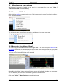
25.1 User specific Toolbars ...................................................................................................127
25.2 Recording Log (Menu "View") ......................................................................................127
25.3 Attributes (Menu "View") .............................................................................................128
25.4 Error log (Menu "View") ...............................................................................................128
25.5 Hardware Settings Viewer (Menu "View") ...................................................................128
25.6 Language (Menu "Extras") ............................................................................................128
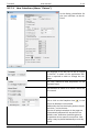
25.7 Settings (Menu "Extras")...............................................................................................129
25.7.1
Import/Export (Menu "Extras") .............................................................................129
25.7.2
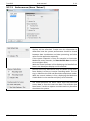
User Interface (Menu "Extras") .............................................................................130
25.7.3
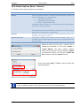
Performance (Menu "Extras") ...............................................................................132
25.7.4
Other Settings: Auto Save (Menu "Extras") ..........................................................133
25.8 Trace Color Definitions (Menu "Extras") ......................................................................134
25.9 Install Options (Menu "Extras") ....................................................................................135
25.10
Import Option............................................................................................................136
26 Group of functions in Formula Editor .......................................................................... 138
26.1 Group "Channels" .........................................................................................................138
26.2 Group "All Functions" ...................................................................................................138
26.3 Group "Base Functions" ................................................................................................139
26.4 Group "File Functions" ..................................................................................................143
26.5 Group "Signal Analysis".................................................................................................148
26.6 Group "Signal Processing" ............................................................................................151
26.7 Group "Filter Functions" ...............................................................................................155
26.8 Group "Programming Functions" .................................................................................157
26.9 Group "Array functions" ...............................................................................................163
26.10
Group "Exponential and Trigonometric" ..................................................................165
26.11
Group "Spectrum (FFT)" ............................................................................................166
26.12
Group "Report Generator" ........................................................................................168
26.13
Group "Recording Parameters" ................................................................................172
26.14
Group "Layout Waveform" .......................................................................................173
26.15
Group "Auto Sequence Functions" ...........................................................................174
26.16
Group "Signal Generations" ......................................................................................177
26.17
Group "Misc. Functions" ...........................................................................................179
27 List of Auto Sequence commands................................................................................ 182
28 Scalar Functions Description Table .............................................................................. 187
28.1 Group "All Functions" ...................................................................................................187
28.2 Group "Vertical" ............................................................................................................188
28.3 Group "Horizontal" .......................................................................................................194
28.4 Group "Periodic" ...........................................................................................................200
© Elsys AG
5
TranAX 3
User manual
3.4.1
28.5 Group "Cursor"............................................................................................................. 201
28.6 Group "Power" ............................................................................................................. 203
28.7 Group "Misc" ................................................................................................................ 206
29 Miscellaneous............................................................................................................. 210
29.1 ActiveX/COM- Interface ............................................................................................... 210
29.2 Sync.Clock Out.............................................................................................................. 210
29.3 Command line parameter ............................................................................................ 211
29.4 Create shortcuts ........................................................................................................... 213
29.5 Block Diagrams ............................................................................................................. 214
29.6 Limitations.................................................................................................................... 216
29.6.1
Digital inputs (markers) ........................................................................................ 216
29.6.2
Differential inputs ................................................................................................. 216
29.6.3
Maximum Sample rate ......................................................................................... 216
30 Trouble Shooting ........................................................................................................ 217
30.1 TranAX Software version.............................................................................................. 217
30.2 TPC-Server Version....................................................................................................... 217
30.3 Driver and Firmware Version ....................................................................................... 218
30.3.1
Example Windows XP ........................................................................................... 219
30.3.2
Example Windows 7 ............................................................................................. 219
30.3.3
TraNET FE .............................................................................................................. 219
30.4 Error Messags............................................................................................................... 220
6
30.4.1
TranAX................................................................................................................... 220
30.4.2
TraNET Config Logfile ............................................................................................ 221
© Elsys AG
TranAX 3
User manual
3.4.1
Introduction
This manual describes the use of Elsys’ powerful hardware, TraNET or TPCX/TPCE modules,
with our Data Acquisition Application and Analysis Software TranAX. It shows all the functions
of TranAX’ operating modes and settings, providing a general overview of the system and its
extensive capabilities.
In TranAX and thus in this user manual, the term "Experiment" is often used. An Experiment
actually must be seen as a project. All the setting, such as amplifier range, sample rate, channel
name, the arrangement of windows, formulas, auto sequences, etc. are stored for a particular
measurement project or "Experiment". Signals are usually stored within this, by the Experiment, managed environment.
When new to TranAX, please have a look at the First Steps.
© Elsys AG
7
TranAX 3
1
User manual
3.4.1
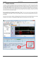
TranAX overview
TranAX is a flexible and powerful tool for utilizing the TPCX/TPCE or TraNET Transient Recorder
instruments for measurement, data acquisition tasks and signal analysis. The software uses the
Windows MDI-interface (Multi Document Interface from Microsoft Windows) that allows several different windows to be created inside the main application window. These sub windows
can be pinned to a tab at the inside of the main window. Each sub window is listed in the View
menu and can be accessed instantly.
Every possible kind of window is listed menu "View". You can create several pages with different Waveforms and tables. Some of the windows can be minimized and attached to the associated page.
As soon as you move a window, docking guides will pop up and let you drag & drop the moving
window on the symbols. Arranging and organizing your workspace hasn't been easier.
8
© Elsys AG
TranAX 3
1.1
User manual
3.4.1
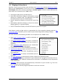
Displays & functions
Basically, TranAX consists of two main windows: the Control Panel and the Waveform Display.
Whereas the control panel is used to set up all the data acquisition parameters and the waveform display shows the currently recording or recorded signals. There are several different displays which are accessed by the "View" menu:





New Page to add several new Waveforms.
New Zoom Waveform Display to add another related
display for a zoomed view. This Waveform just shows
the selected area from the related Display.
New XY Waveform Display to show the XY view of signals
New Marker Waveform Display to show the markers
(digital signals) in a separate display
New FFT Waveform Display to show the frequency spectrum of signals
Each display is within a Page, which is a placeholder for all the waveform displays and the Scalar function table. Therefore, you first have to open a New Page before adding a display.
For more functions, the following windows can be opened in the "View" menu:










New Scalar Function Table A, used for calculation of
values for several traces
New Scalar Function Table B, this table is suitable for
calculation of curve parameters for each channel individually.
New Harmonics Table determines the fundamental
and the harmonics of a periodic signal.
Control Panel, to set up the hardware parameters.
Signal Source Browser gives you access to actual records or previously stored files. Drag & Drop traces to
the waveforms.
Use Formula Editor to analyze and calculate your acquisitions
Use Auto sequences to automatically repeat a sequence of operating steps
Recording Log: Add event comments to your measurement and get an overview of all occurred trigger events. Add own comments for continuous- or ECR Mode. Entrys may also be
made afterwards.
Attributes: Add comments and supplementary information to your records. E.g. Test number, conditions, name of participants.
Error Log lists all relevant program operations and errors occurred
© Elsys AG
9
TranAX 3
1.2
User manual
3.4.1
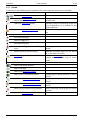
Icons
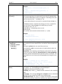
Furthermore, the following quick symbols for the most important functions are included:
Control Panel
Remark
Open the Control Panel
Open the TPC Finder-Dialog, Redefine To connect to other devises in the same
device connections
Network area.
Open the Auto Setup dialog
Automatic setup of measuring range and
view of Waveform, as a function of the
signal-amplitude.
Open the Signal Source Browser
Access to all Signals, also loaded from
files.
Recording Commands
Start Recording (F6)
Manual Trigger (F7)
Stop Recording (F8)
Start a Recording via external TTL-Signal For wiring, please see the Hardware User
input
Manual
Status-Display of the Recording
Additional animated figure, to the status
bar in the lower left corner
Averaging
Summation Averaging over 2 - up to XX
multiple records (usable only in Scope
Mode)
Layout Control
Add a new SCOPE Window
Add a new Page.
Add a new Waveform Display.
Add a new FFT Waveform Display
Add a new Scalar Functions Table A.
Add A new Scalar Functions Table B.
Move Cursors A and B simultaneously
Configuring the default position in menu
"Extras".
Configuring the default position in menu
"Extras".
Configuring the default position in menu
"Extras".
Cursors (normally A and B) will be moved
together.
Opens the Formula Editor
10
© Elsys AG
TranAX 3
User manual
3.4.1
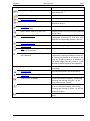
Save Options
Save all Settings
Hardware settings, Layout, Formula and
Auto-Sequence
Load all Settings
Save Traces as TPC5
Equal to HDF5 standard
Save Spectrum, TPS5 Format
Data needs to be calculated in Spectrum
waveform before
File Export, save Traces (TPC-, DIAdem- TPC Files as in TranAX version 2
or ASCII-format)
Export Scalar Table to a ASCII-File
Creates a text file from the actual selected
Scalar Table
Save an entire Page
The sources of the displayed curves are
substituted references so that they then
show the corresponding curves in the file.
Load an entire Page
Print preview
Allows for configuring print layouts.
Print a page according to the configuration in Print preview
Snapshot, copy the actual Waveform to Via menu Extras / Settings / User Interface
the Clipboard.
/ Snapshot, various parameters can be set.
By clicking the mouse on the arrow in the
icon, the screen content of all windows in
the actual page (not only trace or scalar
windows) can be copied to the clipboard.
Block Jumping
Mostly used for Multi block- and ECRrecordings.
Previous Block
Time window moves to previous block.
Next Block
Time window moves to next block.
Lock Cursors on display
Cursors are locked to display, also during
zooming and moving of curves, i.e. are
note locked to the Traces!
Time window marker on the main waveform, are locked to display, also during
zooming and moving of curves, i.e. are not
locked to Traces!
Set time window marker at the border of a
block.
Lock Time Window
Fit Time Window to Block
© Elsys AG
11
TranAX 3
User manual
3.4.1
Miscellaneous Icons
Undo the last view-change of the Waveform display.
Redo the last view-change of the Waveform display.
Pin option to minimize or attach a tab
page
1.3
Only effects zooming and moving of traces on display
Only effects zooming and moving of traces
on display.
Experiment and Settings Information
In the title bar of each window from TranAX, the name and the path of the actual used Experiment-file is displayed. The currently loaded Experiment, the used layout, the file name of the
Auto Sequences and Formula editor are provided as well.
12
© Elsys AG
TranAX 3
2
User manual
3.4.1
First Steps
This chapter is an introduction to the almost unlimited record and analysis features of
TranAX.
For applications where these special features are not required, we direct you to the so
called SCOPE-application.
This chapter "First Steps" will show you how to record from two channels and how to analyze
and save the recordings. It's also assists in understanding some basic workflows.
First, we will do a prepared simple Experiment followed by introducing you to TranAX step-bystep.
2.1
TPC Finder
Before starting measuring and recording, TranAX has to be connected to a device, either
TPCX/TPCE modules in a local computer or external devices like TraNET FE or TraNET EPC. The
communication between TranAX and the devices is based on TCP/IP, so every TraNET device
will be addressed with an IP-address and a port number.
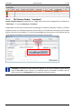
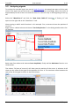
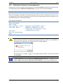
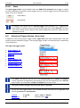
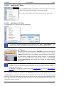
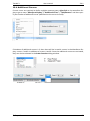
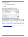
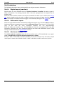
At the first start of TranAX, the windows TPC Finder (Search devices) opens. Click "File" / "Redefine device connections" to open this dialog again for switching to another device.
The current active connection will be highlighted in dark blue; other devices on this list are
available in the network, but not connected.
In case of switching to another device, select one from the list and click the button "Connect".
TranAX will be restarted and the connection to the new device will be ready. If a device has no
connection to the network anymore, the Control Panel switches to orange and notifies of an
error.
© Elsys AG
13
TranAX 3
2.1.1
User manual
3.4.1
TPC Device Finder: "Localhost"
Locally installed modules (TraNET PPC or TraNET EPC) will not be managed by its IP address in
"TPC Finder". It is stored directly as "Localhost".
Independent of the current status and the topology of networks (company network, customer
network or even no network connection) after startup of TranAX the connection will be made
directly with the local modules. This has the advantage that connection to the devices will be
made without any detour through other existing network connections.
"Localhost" references to the internal IP address of the local computer, which will always be 127.0.0.1. Even if there is no network device or hardware installed, this address exists and is independent from the general network settings.
14
© Elsys AG
TranAX 3
2.2
User manual
3.4.1
Simple Experiment
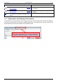
Load the Experiment "FirstSteps" with "File" / "Open Experiments". You may browse through
the directories to find the Experiment. Depending on the version of Windows, it's possible the
folders have different names.
Load the settings FirstSteps_Scope1.lay with "File" / "Load all settings".
By connecting simple wires to the BNC connectors A1 and A3, one can generate EMI signals
(electromagnetic interference). You also may connect another signal source, e.g. a function
generator.
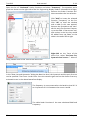
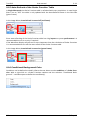
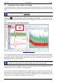
Hit the start button
to start the recording. Because we enabled Auto Trigger and disabled
Single Shot in the Control panel, the Waveform display shows continuously the newly recorded
signals.
To stop the recording, hit the stop button
© Elsys AG
.
15
TranAX 3
User manual
3.4.1
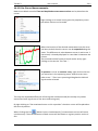
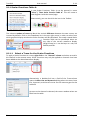
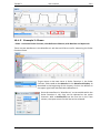
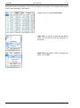
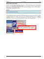
In order to display each channel in a separate
part of the waveform, right-click on the waveform background and set "Number of Areas"
to 2.
Move the second trace from the upper part into the lower by Drag & Drop. Place the mouse
pointer over the trace indicator rectangle (little colored boxes to the left of the waveform display) and click it with the right mouse button.
16
© Elsys AG
TranAX 3
2.3
User manual
3.4.1
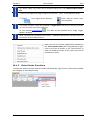
Starting a own recording (setting up the Control Panel)
Before we start a new recording, we will change some hardware parameters (sample rate,
block size, time basis...) in the Control panel. ("View" / "Control Panel" or use the control panel
icon
). Select the first three channels in the control panel list (A1 to A3). Each list entry
corresponds to a channel from a TPCX/TPCE Module.
Main settings: We will leave the operation mode at Scope mode (default mode). For more information about the operation modes settings look at Main settings section. And for more detailed information how these modes work go to the Signal Capture Principles.
We set the sample rate to 200 kHz. Type 200k in the Sample Rate text field or use the
dropdown list. For the Block Size, we set 8 kS (kilo samples). Just below the block size setting
we see the resulting recording Time Window. In our example we doubled the sample rate and
reduced the recording length by halve. Therefore the recording time window results in a forth
of the previous value. Finally, for Trigger Delay we set -10%.
On the Input Amplifier tab we just change the Range to 10V and leave the Offset at 50%.
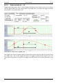
We go on with the Trigger tab. We choose the Slope as Trigger Mode and we want TranAX to
trigger if a positive rising slope to a level of +1.5V has been reached. Therefore, we select the
+Slope comparator, set the Level to 1.5V and the Hysteresis to 0.2V. You also have to activate
the Enable checkbox.
If a different unit then Volt is required, choose the Physical Unit option. Since we chose Volts
for our recording, we will not change the Physical Unit.
Now we have configured the channels from A1 to A3 similarly. Later, we want to record signals
triggered on the positive slope of the channel A1 or on the negative slope of the channel A3.
Select the channel A3 in the list and go to the Trigger tab and change the comparator to -Slope.
Set the Level to -0.5V and the Hysteresis to 0.2V.
© Elsys AG
17
TranAX 3
User manual
3.4.1
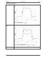
We now are ready to initiate a new recording. In advance you should remove the signals at the
BNC inputs. To start recording, you either hit the red start button
in the control panel, on
the tool bar or simply hit F6 on your keyboard.
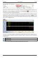
TranAX will display the message Recording active in the message bar which is placed in the bottom left corner. Now, connect a rising signal (>1.5Volt) to input A1. As soon as trigger has been
released the recording will be terminated and the message bar will display "Stopped". In the
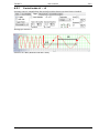
upper waveform part you can see the recorded signal from channel A1 with a rising slope up to
over 1.5Volt at triggered event.
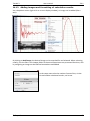
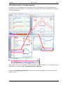
The trace is not optimal placed in the waveform window because we have changed some recording parameters (sample rate, block size, amplifier range). To adjust the curve, click the following buttons:
Full scale Y axis
Full scale X axis
Now we can zoom in again by selecting the area with the mouse cursor.
18
© Elsys AG
TranAX 3
User manual
3.4.1
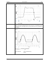
Remove the connection on input A1 and connect a signal with falling edge of < -0.5V on input
A3. Now another trigger on channel A3 should initiate the end of the recording. In the lower
Waveform part you can see the recorded signal of the channel A3 with a falling slope under 0.5Volt at trigger time.
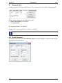
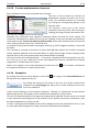
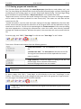
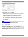
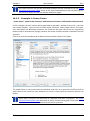
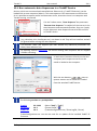
2.4
Saving recordings
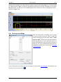
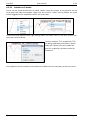
After we finished the recording, we are going
to save the two curves to a file. To save the
actual recording, go to the menu "File" / "Save
traces as tpc5". Select from the left field Available the channel 1 and 3 and move them to
right field Selected. Leave the other settings as
they are. For more information about the saving options, please have a look at the Saving &
Printing section.
As we finished the recording, we are no longer in need of the Control Panel. So therefore, we
minimize it via the pin button
.
© Elsys AG
19
TranAX 3
2.5
User manual
3.4.1
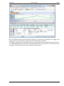
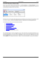
Analyzing signals
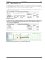
To analyze the recorded signal, we use the Scalar functions. As example we want to find a peak
value in the signal, we set the cursor A and B in the waveform accordingly. Move the cursor B
approximately to end of the curve and the cursor A to the left resp. to the beginning of the signal.
Select the "Waveform 1" and click the "New Scalar Table A" button
opens on the right side to the "Waveform 1" tab.
. A "Scalar_A 1" tab
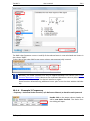
We are going to add 3 scalar functions in this example. First, we want to know the position of
cursor A.
Right-click on a None-column and choose "Set Scalarfunction". In the dialog window select Cursor Position.
Redo steps from above and choose Cursor Amplitude, finally add the Maximum function to a
third column.
The column TA (time of cursor A) will show you the position of the cursor A, whereas A will
show you the value of the signal at the position of Cursor A. The maximum value between the
two cursor of the signal is shown in the third column.
20
© Elsys AG
TranAX 3
User manual
3.4.1
To analyze the curve of channel A3 you have to right-click on a free line in the "Trace" column
in the scalar table and navigate to "Channel" / "0A3".
Then you have to place cursor A and B to a desired new position. The scalar function searches
the Max value between the two cursors. If the cursor are outside of the window you can move
them with the right mouse button and select Place/Cursor x. Note, the mouse symbol should be
set in advance on the X-position in the window where you would like the cursor to be placed.
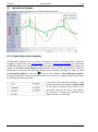
Finally, we show you how to analyze previously saved signals. The signal of a TPC5 file can be
accessed via the Signal Source Browser. Use the button
if the window isn't opened yet.
Then open the file by clicking on the file open button in the upper right corner. Perhaps you
have to navigate to other directories to get the desired file listed.
To display the saved signal on a separate display, right-click on the waveform and choose Number of areas/3. Now, you can place the file signals via drag & drop in this new display and hit
the Full Scale X button
.
As you might have realized, the signals from the file allocates a larger time region then the actually recorded signals because we changed the time relevant recording parameters for the
new actual record. Normally, TranAX can handle such different records without limitations. Also
you can perform any calculations on file signals in the same manner as on current recorded
curves.
© Elsys AG
21
TranAX 3
3
User manual
3.4.1
SCOPE (Oscilloscope)
With SCOPE, instrument handling in straight forward applications has become much easier, as
TranAX behaves like an oscilloscope that way. Although still without rotary knobs, the elements
of seldom used operating modes are moved significantly to the background.
All manipulations, whether it concerns waveform curves and their windows, axes, annotations,
etc. all behave as in a normal TranAX Y/T Waveform window.
By clicking on this icon
3.1
a SCOPE display will come up.
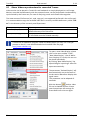
Channel settings
In the lower part of the display each hardware channel has its operating box.
Depending on the available hardware (channels) 4 to 8 such boxes are available (in systems
with more than 8 channels only the first 8 will be shown).
The operating box for the first channel (BNC A1) is at left. These boxes are typically labeled with
the name of the channel.
A yellow square is drawn around the entire operating box
when the mouse cursor is on the area. Left clicking the
mouse activates or deactivates the channel. By activating the
channel also the curve will be shown.
22
© Elsys AG
TranAX 3
User manual
3.4.1
When the mouse cursor is over a channel name, a yellow square is
coming up. Left clicking opens a menu for setting up the most important channel parameters.
A yellow square also will come up, when the mouse cursor is
placed over a scalar value. By left clicking the mouse a menu is
coming up for selection and specifying of a scalar function.
3.2
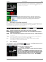
Buttons for recording commands
In the upper part of the display are the recording command buttons. As mentioned these emulate oscilloscope operations. More advanced recording modes (e.g. Multi-Block, ECR, etc.) are
still possible but via alternative set-up procedures.
Auto:
Multiple record mode with “Auto Trigger“ (free running oscilloscope).
Normal: Multiple record mode by waiting for a trigger, then finish record and start again for
waiting on next trigger, etc.
Single: Starts record and waits for triggering, finishes record then stops. Needs re-arming for
next record.
Trigger : A software trigger is sent to the hardware. A running recording can be finished orderly that way e.g. in the case of a missed signal trigger.
Stop:
A running recording will be stopped. Then waiting. Normally such recorded
signal cannot be used for further processing.
3.3
Time settings
Time range can be set with the Time Window parameter. After a recording its value usually will
be equal to the full range of the X-axis (button
down left).
The time range is calculated as follows:
T = Blocksize * 1/Samplerate
The user has the choice which of the two values should be set as
a constant.
By clicking on the Timebase box (below right) a menu will come
up. There a fixed sample rate or fixed block length can be chosen
within their proprietary ranges. Then the other value will automatically be calculated in relation to the set Time Window parameter.
© Elsys AG
23
TranAX 3
User manual
3.4.1
With Trigger Delay actual pre- or post trigger values (-100% to +200%) can be set. Those settings however influence the range of the time axis. In any case also via
the full range of
the X-axis can be set .
3.4
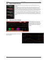
Trigger conditions, trigger level
Trigger conditions are also set via the channel settings menu. They are deliberately kept simple,
i.e. only edge and window triggers can be set.
Other adjustments (incl. Trigger-option modes) if need can be set directly in the control panel.
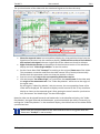
Trigger level is being set directly in the waveform window. For every active channel which trigger mode is not
set to OFF, at the left and right side of the waveform window triangle symbols appear. They can be grabbed with
the mouse and moved vertically. These symbols also
show whether triggering will be on a positive or negative
edge.
Window triggering is shown through two (four) halftriangles. Those also can be picked up by the mouse and
shifted up or down.
In case the level is set outside the vertical range of the
signal, a warning triangle will appear. Its meaning is that
on this channel no trigger can be generated.
In case the level is set above or below the display window
(as a result of Y-zoom) white arrows appear, pointing to
where the trigger point is. They can be picked up by the
mouse and trigger point dragged into the display.
When these symbols are left clicked instead of grabbing,
the menu for channel settings comes up (similar to clicking on channel names in the channel operating box).
24
© Elsys AG
TranAX 3
3.5
User manual
3.4.1
Digital ReadOut Boxes
On the right hand side of the display several ReadOut Boxes may be
shown.
By clicking on the vertical bar at right, they will be switched on or off.
The digital measurement values are obtained through scalar calculations. In principle all calculations as per the Scalar -Table B are possible.
The values are labeled with abbreviated measurement/calculation results as well as channel names. If a calculation is carried out on a curve
in a file, then also the name of the file will be blended in . Right clicking on the label overhead, opens the menu for selecting scalar calculations.
3.6
Maximum curve display
Left clicking on the top or bottom horizontal bar, suppresses
operating tabs at the top as well
as the channel operating fields
below.
With that additional space for curve display is created.
© Elsys AG
25
TranAX 3
4
User manual
3.4.1
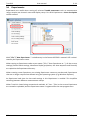
Control Panel
The control panel is used for setting up data acquisition parameters such as sample rate, input
voltage range, etc. This window is presented in two sections:
The upper section contains a table, which lists the current setup for all the channels. The channels are recognized automatically at program start. The table allows the user to select one or
more channels in order to modify the setup. By pressing and holding the left mouse button and
moving it over the desired channels you can easily select several channels at once.
This method will not work if the mouse cursor is placed over the first two columns. These two
columns are reserved for moving channels to the waveform display by drag & drop
The upper part of the Control Panel can be saved to a text file. Select the channels as
described above and press <Ctrl>+s to open the Save File dialog.
The setup for the selected channels is presented in the lower display section of the control
panel. The channel parameters can be modified by selecting the relevant tabs.
26
© Elsys AG
TranAX 3
4.1
User manual
3.4.1
Main settings
With a TranAX data acquisition system (transient recorder) it's possible to measure fast signals
(transients), but also slow, sporadic and periodical signal.
The basic hardware contains 4 or 8 channels. Depending on the Computer you are using, it's
possible to add up to 64 channels per system.
Signals will be recorded parallel, for every channel its own data array will be used, independent
of the memory size of the computer. Trigger events can be set individual for each channel; it's
also possible to combine these events logical.
The "Main" tab contains the following configurable time base parameters:
 Operation Mode:
o Scope (with auto trigger and/or single shot)
o Multi Block
o Continuous
o ECR (Event Controlled Recording)
 Sample clock source: internal or external
 The sample rate (internal clock) or expected clock frequency (at external time base, used for
some time related data analyses functions)
 The measurement length (block size with pre- and post-trigger)
 Trigger delay (defines relation of pre- and post-trigger)
By the Button "Armed / SyncOut" the corresponding output on the Digital Connector can be
switched as Armed Out or as Clock Pulse Output with settable frequency. This frequency is independent of the set Time Base Rate. This signal may be used as syncronisation of external devices (e.g. Highspeed Cameras).
At older devices this button may not be present. Such devices have to be updated at factory.
© Elsys AG
27
TranAX 3
User manual
3.4.1
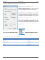
The sample rate can be set and displayed using either frequency or time period. The input field
will accept the following short form (u for micro, m for milli, k for kilo, M for mega) and for units
(H or Hz for Hertz, s for seconds). Example:
Input
Interpreted as
Input
Interpreted as
10k
10 kHz
15u
15 µs
2.5M
2.5 MHz
500Hz
500 Hz
2.5m
2.5 ms
3s
3 sec
The data acquisition time (Time Window) depends on block length and sample rate.
4.2
Icons
The command buttons to the left of the setting tabs have the following functions:
Start a measurement (F6).
Alternatively, the data acquisition can be started by an external TTL-signal and by enabling external start by a click on the corresponding icon
in the icons list.
Manual trigger (F7)
Stop measurement manually (F8)
Load setups
Save setups
Display Hardware Configuration (information window)
Display Cluster Configuration
4.3
Control Panel tabs
To change the settings use the dropdown and option lists. Text fields can either be set manually
by typing your desired value into it or by the following two buttons:
In/decrease the value by a given step
Choose values from the appearing list.
Switch the parameters which you want to edit.
Some settings will be displayed in a small illustration next to the settings. You then also can
change the settings by moving the markers in the illustrations, e.g. Trigger Delay
You can save the entire hardware configuration with "File" / "Save recording settings" or by
clicking on the button
28
on the left side of the Control Panel.
© Elsys AG
TranAX 3
5
User manual
3.4.1
Reference Pointers
From TranAX version 3.4.0.1200 onwards it is possible, instead of curves from files to work
with so called Reference Pointers. Hardware channels can be assigned as well to these pointers.
With pointers it is possible to sequentially analyze single Tpc5 files that for example have been
recorded in Auto Sequence mode. The reference pointer can be imagined as a place holder that
can be used in a Waveform Display, Scalar tables or Formula editor. By assigning curves from a
different file (or hardware-channels directly) only the data content is exchanged, while the profile (color, line thickness, zoom position, labels, etc.) will be retained.
This offers the advantage that the planning and preparation of a screen lay-out, e.g., curves
display, scalar tables, texts, only once needs to be set up with the Reference Pointer curves.
Subsequently all measurement curves can be assigned via Drag & Drop, without having to replace those in the lay-out or in a formula each time.
Copy files are not generated. The Pointer acts like an arrow referencing a selected
Signal Source (file or hardware channel).
When such a source file is removed from the computer or moved then that pointer
disappears, e.g. is empty.
5.1
Potential Sources for Reference Pointers
Handling of the Reference Pointers takes place in the Signal Source-Browser (
).
The Pointer Fields are found in the Signal Source
browser next to the file-tree. They are visible by clicking the vertical grey bar on the right.
By clicking on the symbol
more fields (empty
for now) can be added.
Only the lowest field can be removed. For that click
on the small "x" in the field’s top-right corner.
To designate a Pointer, the desired object (an entire
file but also just single curves) can be moved onto a
Pointer-field through Drag & Drop. Then, normally
this Pointer-field will be moved via Drag & Drop, into
a curve display.
© Elsys AG
29
TranAX 3
User manual
3.4.1
The following objects are valid:
 Stored files, with the following formats being supported:
o *.Tpc5: TranAX 3 Standard Format for measured curves in time domain
o *.TPS5: TranAX 3 Standard Data Format for Spectrum and FFT curves
o *.TDP: stored Tab-Pages in TranAX 3
o *.BDF: binary Raw Data from Recorder and ECR-Mode
 Hardware Channels, all channels on the Control Panel respectively from an actual cluster. Thereby it is also possible to select multiple channels from the two first columns and
via Drag & Drop deposit those on a Pointer-field.
 Averaged YT and FFT curves (@- resp. %-curves) several channels here as well can be
selected and dragged onto a Pointer-field.
The designated Pointer-fields then can be via Drag & Drop moved onto a curve display. This
relates always to all the curves designated to a given Pointer. When, for example only one
curve is being dealt with, only that curve should be dragged onto the Pointer-field.
5.2
Reference-Pointers in the Formula Editor
Pointers can also be used in the Formula Editor.
With the File-command a curve in a Pointer-field can be accessed
trace = File(ref1,index) [.blkNo] ['markerNo]
The index designates the curve in the file (0...). Rather than to provide the full file name in the
quotation mark only the term ref with the corresponding number needs to be given (e.g.
"ref1").
In case only the first (no: 0) curve in a Pointer needs to be accessed, the formula also can be
simplified:
trace = ref2 [.blkNo] ['markerNo]
This command relates to trace=File(ref2,0)
Optionally, identified Block- and/or Marker-numbers also can be allowed.
Likewise the following functions are permissible:
val = FileIndexExist (ref1, 2) ; val = True or False
nTrc1 = NTracesInFile (ref1); is synonymously to Length (ref1)
nTrc2 = Length (ref2)
Ref, in the formula editor is used as a key-word.
30
© Elsys AG
TranAX 3
5.3
User manual
3.4.1
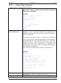
Reference-Pointers in Autosequence
Pointers also can be used with Auto Sequences. At command Save instead of the file name, the
corresponding Pointer (without name extension, e.g. TPC5, etc.) must be indicated.
Save ref1, 0A1–4
With this method it is possible in an Auto-Sequence-loop to archive measured curves (in number-progressive files) and simultaneously use the actual measurement data for display or extended calculations in the Formula editor.
Auto Sequence example:
Repeat 10
Start Recording
Wait on EOR
Save xy_#.tpc5, 0A1-4 ; Generate a measurement series
Save ref4, 0A1-4
; Generate (overwrite) a file
; "ref4.tpc5" and allocate to the
; corresponding Pointer
Calculate
Wait for Calculations
Next
The expression "ref" serves as keyword and is accordingly checked!
When a Pointer-field with the corresponding number (e.g. "ref4") is not available in
the Signal Source Browser, the following error message appears:
By clicking on the symbol
can be added.
in the Signal Source Browser, more Pointer-fields
In Auto Sequence mode the curve is stored physically as a file (e.g. "ref1.tpc5") in the
"data" register of the actual Experiment and assigned to the corresponding Pointer.
© Elsys AG
31
TranAX 3
User manual
6
Operation mode
6.1
Scope
3.4.1
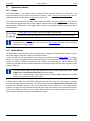
The Scope mode is the default mode. No data will be actually stored to the hard disc. The
measured data is only present in the channel memory. After starting the measurement the actual block will be shown when a trigger event occurred.
In this tab you can set the time base, the sample rate, block size and trigger delay. The illustration below the trigger delay entry field shows a representation of the trigger point in relation to
the complete measurement. The trigger delay can also be set graphically by moving the box in
the illustration.
If no trigger event occurs TranAX will trigger automatically.
Only one shot will be displayed and the measurement will not be continued.
If more than one cluster is configured, the Single Shot checkbox is always on, auto
recording start is not possible. You may use an Auto Sequence with "start recording"
command in a loop instead.
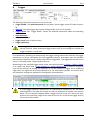
6.2
Multi Block
The Multi Block mode will store signals sequentially in segments of the channel memory. Therefore each trigger event will initiate a new block of data.
In this tab you can set the time base, the sample rate, block size and trigger delay. The trigger
delay can also be set graphically by moving the box in the illustration. In addition to the scope
mode the number of blocks respectively the number of measurements can be defined. The
maximum possible number of blocks depends on the block length and the total capacity of the
onboard memory.
The Multi Block Mode is specially designed for burst-mode applications with a fast
trigger rate and minimized dead-time between Blocks.
In case it is a requirement to have dead-time free burst mode acquisitions, the ECR
Mode is the ideal data acquisition mode.
In Multi block mode, the TPCX/TPCE modules take over full control of measurement process
and data storage (channel memory). The measurement will be allocated to a block size which
matches the available memory. The only involvement of the computer in the measurement
process is to give the start command and then wait until the hardware has completed the task.
The PC then reads the data. For this reason block mode is the simplest mode and doesn't require complex settings for quick and satisfactory results.
32
© Elsys AG
TranAX 3
User manual
3.4.1
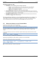
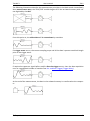
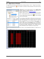
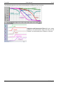
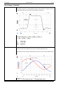
The following illustrations describe the measurement principles in the block mode. Immediately
after measurement start, the TPCX/TPCE module begins to fill the on-board memory with values digitized by the ADC.
From this point on, the oldest data will be overwritten by new data.
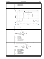
If a trigger event occurs, the current sampling stops and all the data is present one block length
prior to the trigger event.
If required to capture a signal before and/or after the trigger occurs, then the data acquisition
runs on a predefined number of samples (see Pre- and Post-Trigger (Trigger Delay).
At the end of the measurement, the data in the onboard memory is transferred to the computer.
© Elsys AG
33
TranAX 3
6.3
User manual
3.4.1
Continuous
In continuous mode the instrument works as disk recorder. No block size or pre/post trigger
settings can be made.
The start is normally initiated by the button
data acquisition.
.There are three possibilities to terminate the
The acquisition will stop when a trigger event occurs. Additionally, a
trailer length must be set. The measurement will then run after the trigger event for a predefined period. The trigger settings are set in the
Trigger tab.
The acquisition will stop after a pre-defined time limit. The Maximum
Record Length depends on the free hard disc capacity.
If the disc capacity is exceeded, no more data will be recorded!
Stop the measurement manually.
If both options are enabled, then the recording will stop when either one of the
events occurs.
If another Cluster detects a trigger, then this trigger would also initiate the stop trigger of the continuous recording!
In continuous mode the measured data is continuously written to the computer where it will
be stored, for example, to the hard disk. The measurement can be stopped either by a signal
trigger event or manually via computer. The onboard memory is used as one large buffer in this
mode.
The measurement length is limited by the hard disk capacity and the sample rate is limited by
the transfer speed between the module and the computer. Depending on the computer specification, the total sample rate can be up to a few tens of mega-samples per second. This maximum rate is achieved when no other applications are running at the same time. The measurement is protected from fluctuations in sample rate or loss of data due to computer loading by
buffering the data through the large onboard memory (up to 64 MSamples/channel). This
measurement mode is intended for data captures over longer periods.
The recording stops automatically if the hard disk gets full.
34
© Elsys AG
TranAX 3
6.4
User manual
3.4.1
ECR mode
The ECR mode is a software option.
The ECR mode allows targeted acquisition of cyclic or sporadically arising events. This implies
that the registration of measuring data only occurs if certain signal conditions (trigger, time
window, repetitions, etc.) are fulfilled. Thus many unwanted and unneeded signal data will not
be stored.
Nevertheless, it can be guaranteed that no dead times arise and therefore no events will be
lost. This even applies if many channels at maximum sample rate have to be supervised over a
long period of time. Since each channel possesses its own signal buffer (up to 64M samples),
only the average number of events per second may not exceed a certain value. This value depends on the adjustable block length per event and furthermore it is defined by the maximum
possible transfer rate to the hard disk (approx. 20M samples per second, depending upon
CPU/Disk systems). The trigger conditions can be individually set for each channel, whereby
even more complex signal criteria (e.g. pulse width/height, slew rate, window-IN/OUT) can be
defined.
Compared to the block mode, with ECR mode it is guaranteed to have no dead times
between adjacent blocks. Note that, if in block mode a trigger event occurs at the end
of the block, the event might not be recorded.
In the ECR-mode it is guaranteed that there is no dead-time between adjacent blocks. The overlapping data-area depends on the event-rate and it can be controlled within certain limits with
the Holdoff function. In Block Mode on the other hand, the blocks are strictly sequential data
acquisitions with a gap between blocks.
If the operation mode is set to ECR mode, an additional ECR tab will be opened. In the ECR
mode the block size is determined explicitly by pre- and post-trigger settings. As with the multi
block mode you also can set the maximum number of blocks that will be recorded. Furthermore, there is a Retrigger (RT) marker in the illustration below the settings or a Holdoff (HO)
marker shown, depending on the settings made in the ECR tab. There are two different ECR
modes, the single and multi channel mode. Both modes support a Dual mode option.
If the trigger conditions are set very uncritically, then in ECR Mode the CPU could easily
be overloaded by fast periodically signals. The CPU might seem to be blocked.
© Elsys AG
35
TranAX 3
6.4.1
User manual
3.4.1
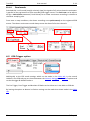
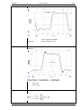
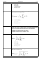
Basic Sequence
The ECR mode runs as follows: The digitalized signal will be stored to the onboard memory
which acts as a ring buffer.
As soon as the trigger is released, a block of samples will be read from the ring buffer and will
be saved to the hard disk.
If a new trigger event within the actual block occurs, a new overlapping block will be saved.
If the ring buffer is full, the oldest measurement data will be overwritten with new incoming
data. Usually, the overwritten data would be transferred to the hard disk before this happens. If
too many events occur in a period of time, the ring buffer may overflow. TranAX will display a
message according to the status.
After the predefined number of saved blocks is reached (in this example 3), the recording stops.
36
© Elsys AG
TranAX 3
6.4.2
User manual
3.4.1
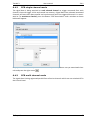
ECR single channel mode
The signal data is being acquired on each selected channel on trigger command from each
channel's internal trigger circuit and stored into memory. Signal data from selected associated
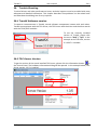
channels will store their data parallel and synchronously with the triggered channel it is associated to. To associate a channel, press the button "ECR Associations" and a window as shown
bellow will appear:
Simply select the desired input channel from the Input-field, choose not yet associated channels and press the right arrow
6.4.3
.
ECR multi channel mode
The signal data is being registered parallel from all active channels which are not switched off in
the Control Panel.
© Elsys AG
37
TranAX 3
6.4.4
User manual
3.4.1
Dual mode
Switched ON, it will record (usually relatively slow) the signals of all active channels continuously parallel to the registration of (fast recorded) ECR trigger events. The clock rate can be adjusted (by a clock divisor parameter, Dual Divisor) for a slower continuous recording in relation to
the faster sampling rate.
From start to stop conditions, the slower recording runs synchronously to the registered ECR
events. The slower continuous record always stores the data of all active channels.
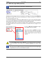
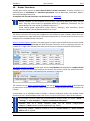
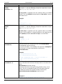
6.5
ECR Trigger option
Additionally to the ECR mode settings which can be made in the Main tab, in the control
Holdoff in the ECR tab you can choose between the Normal, Retrigger and Holdoff options and
set the Retrigger & Holdoff markers.
The Pre-Trigger, Post-Trigger and Number of Blocks can be either set in the Main or ECR tab.
By leaving the option at Normal no further settings can be made than those made in the Main
tab.
38
© Elsys AG
TranAX 3
6.5.1
User manual
3.4.1
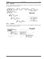
Normal
With the additional trigger settings Retrigger or Holdoff the recording of an unwanted number
of overlapping blocks can be avoided.
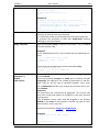
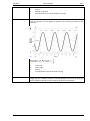
6.5.2
Holdoff
With the Holdoff control set to Holdoff, you can instruct TranAX to ignore all additional trigger
events until to the Holdoff marker HO.
© Elsys AG
39
TranAX 3
6.5.3
User manual
3.4.1
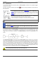
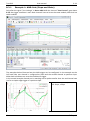
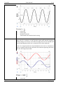
Retrigger
Choosing the trigger mode Retrigger with the Holdoff control you can set the retrigger mark in
sample lengths or in time measurement. Contrary to the Holdoff option, trigger events will be
ignored to be recorded, but as soon as a new trigger event occurs, the retrigger marker RT will
be moved on and set newly relatively to the new trigger event (respectively retriggered). Only
after the retrigger marker is passed, a new block will be stored. Additionally, a maximum Post
Trigger block length can be set. TranAX will trigger according to the illustration below:
40
© Elsys AG
TranAX 3
7
User manual
3.4.1
Input Amplifier
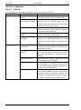
The following channel parameters are set in this tab:









Mode: Single Ended (screen to ground), Differential or Off
Input coupling: DC, AC or ICP (Integrated Current Power for Piezo sensors). For the modules
120MS and 240MS modules, the input impedance can be set to 50Ω. For all other modules,
this value is set to 1MΩ.
Input voltage range: Total range and offset
Filter: Incl. Anti-Aliasing filter, (optionally available)
Input inversion
Channel name
Averaging: Off, 14Bit or 16 Bit
Marker name (optional digital inputs)
Marker signal inversion
The above values may be set for each individual channel. All installed channels are detected at
program start, these are then included in the table.
7.1
Averaging
The ADC runs always with the maximum possible sample rate. If the selected sample rate is
less than the maximum rate, then the excess samples will be averaged. This way the signal to
noise ratio is improved correspondingly. For applications which don’t allow averaging (e.g. under sampling recording), it can be switched Off.
The parameter "Averaging" will be set for all channels within a module.
In some cases, averaging should not be used, e.g. for under measuring (sampling with
a lower frequency then the measured signal). In this case, averaging has to be set to
"off".
7.2
Amplifier options
The input voltage range settings are defined in two parts: Range and offset. The range sets the
maximum possible data capture voltage amplitude. The offset sets the zero point of that range
and therefore the absolute minimum
and maximum voltage limits. These limits are displayed both in the data input
field and in the table. Each input channel can be set to operate in inverted
mode i.e. the polarity of the input voltage is inverted. Each channel can be given a name in order to identify it with its relevant signal.
© Elsys AG
41
TranAX 3
7.3
User manual
3.4.1
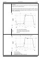
Markers (Digital Inputs)
Every data acquisition channel has two digital inputs called Markers. Marker signals are digital
signals with values 0 or 1 and they can be displayed in the dedicated Marker Waveform Display.
The controls "Marker 1" and "Marker 2" allow defining names for the digital input signals. In
case Invert is selected, the marker will be inverted before it is displayed. This is useful in cases
of signal inversion, for example, with opto-couplers. Also see the chapter on Limitations / Digital Inputs (Markers).
Marker inversion will be marked with a "\" (Backslash) at the end of the name.
"M1\" means the inverted Marker 1.
In case the TPCX/TPCPE digitizer module is set to 16-bit mode, there are no Markers
(digital inputs) available.
These settings are always visible in the Control Panel, even when there is no Marker
option installed.
The corresponding analog channel must be switched ON (tab "Input Amplifier" in the
Control Panel) to record the Marker signals.
42
© Elsys AG
TranAX 3
8
User manual
3.4.1
Trigger
The following channel parameters are set on this tab:
 Trigger Enable: The selected channel will only be an active trigger source if Enable is selected.
 AND Link: The AND trigger logic can be configured per 4-ch or 8-ch module
 Trigger Mode: See "Trigger Mode" section for detailed information about the operating
modes
 Input Multiplier
 Comparator (Slope)
 Trigger Level [Volt or Physical Unit]
 Trigger Hysteresis
The trigger condition is one of the most critical settings. If the trigger conditions are
not set correctly, either unwanted trigger events occur or the settings are invalid so a
trigger condition is never met.
If no satisfactory recording can be achieved, the trigger settings need to be checked. The trigger
parameters can be set individually for each triggerable channel. At program start the software
automatically identifies which installed channels are triggerable. The triggerable channels have
entries in the table under Trigger Mode and Level.
Depending on the selected trigger mode, either level and hysteresis (+ Slope, - Slope, ± Slope)
or an upper and lower level (Trigger Window in, Trigger Window out) in volts or in physical
units can be defined. By setting the hysteresis it can be avoided to trigger on an undesired
edge, when the signal has noise superimposed on it. For information purpose, the current level
and hysteresis settings are displayed in small graphic representation.
If in the trigger setup of a channel e.g. an invalid level or hysteresis is set, the corresponding field in the table will change its color to yellow/red as shown in the picture
above. This for example happens when a trigger level of, let say 1V is set for an input
and then the sensitivity range of this input is set to 0.5V. In this case a trigger level of
1V can never be reached.
© Elsys AG
43
TranAX 3
8.1
User manual
3.4.1
Input multiplier
The function Input Multiplier multiplies the currently digitized signals of two channels (e.g. A1
and A3 or A2 and A4). The resulting signal (a product) will then be passed to the trigger discriminator instead of the original signal from channel A1 resp. A2, on which the module will trigger.
The range and resolution of the products depend on the settings (range, offset, physical scaling
factor and physical unit) of the two channels.
The full range and full resolution can only be exhausted to half. This will be the case if both
channels are set to 0% or 100%. The multiplied product curve will then have a range from 0 to
+Max or to -Max. There will never be a multiplied product in a range form -Max to +Max. Having the offsets set to 50%, only one fourth of the maximum possible resolution is achieved.
Note that the hardware multiplier doesn't take the constant of the Physical Scaling
into account. It should therefore be set to 0 for both channels.
The checkbox "Store product" only visible when "Input Multiplier" is activated will replace the
recording of one channel (e.g. A1) with the result of the multiplied two channels. The second
channel (e.g. A3) will contain the normal recording (unchanged).
The amplitude resolution of the product signal is also 14-bit resp. 16-bit. If the original signals
don't use the full dynamic range of the amplifier and the ADC, the resolution of the output signal can be strongly minimized. It's recommended to choose for both signals, measurement
ranges that optimize the dynamic range of the input stages.
44
© Elsys AG
TranAX 3
8.2
User manual
3.4.1
AND Link (logic AND operation)
AND Link is a feature of the TranAX option "Advanced Trigger".
By default, all active trigger sources are combined in an OR-logic. This means, any enabled trigger source can trigger all the channels simultaneously of a TraNET instrument or a TraNET system synchronized with Sync-Link.
In cases where AND-logic is required, all trigger sources of a 4-ch or 8-ch TPCX/TPCE module,
e.g. A1 - A8, can be combined in an AND-logic. Therefore the AND Link needs to be activated on
those channels of a module that need to form the desired AND combination.
The AND-logic trigger allows to combine all trigger modes, including the AND Link dedicated
State trigger mode, across all channels of one module. This enables the user to trigger on complex signals.
As soon as AND Link is activated the trigger
mode "State" becomes available.
State can be used as a qualifier for another
trigger source. Only if the State of a trigger
source is met AND when the conditions of
another trigger source are met, it will be
triggered.
If only one trigger source is set to "AND Link", it acts exactly the same as in OR logic.
To use this function, there needs to be at least two channels with enabled "AND
Link".
While the default OR-logic works with all the channels of a Transient Recorder system across up to 8 TraNET instruments synchronized with Sync-Link, the AND -logic
is applicable just to a 4-ch or 8-ch module in a system.
© Elsys AG
45
TranAX 3
8.2.1
User manual
3.4.1
Example 1: AND-link (Slope and State)
Only after the signal "Line Voltage" is above 100V AND the channel "Line Current" goes above
0.5A, the trigger condition is met. Both channels have to be on the same module, AND Link has
to be enabled.
The examples below illustrate how the AND trigger can be configured. In the example on the
left hand side, one channel is configured as State and the second channel as positive slope.
When both conditions are true the module will trigger.
In the second example channel one is watching out for pulses smaller than 1us and channel two
just for a simple edge trigger of a positive slope.
A1: +Period<t, t<1us;
A2: Slope, +Slope
46
© Elsys AG
TranAX 3
User manual
3.4.1
The Control Panel shows the current trigger configuration in the columns Trigger Mode, Link,
Level and Hysteresis. All settings are performed in the Trigger tab.
8.3
Pre- and Post-Triggering (Trigger Delay)
Pre- and post-trigger is applicable to Scope-, Multi Block- and the ECR mode. The position of the
measurement window (or block) can be adjusted relatively to the trigger point within limits. If
it is required to capture a signal prior to the trigger point, this is called pre-triggering. Conversely, if it is required to capture a signal after the trigger point it is called post-triggering. These
trigger delays (-% for pre; +% for post) are defined in terms of percent of the total block period.
The TPCX/TPCE hardware allows a trigger delay between -100% and +200%.
Trigger delay (trailer)
There is no pre/post trigger in Continuous mode. In this mode the stop trigger and trailer are
utilized. The stop trigger is used to determine the end of the measurement i.e. data acquisition
stops at trigger. However, sometimes it is required that the measurement continues for a predetermined time after the stop trigger - this is called the trailer. The trailer is defined in number
© Elsys AG
47
TranAX 3
User manual
3.4.1
of samples after stop trigger. The TPCX/TPCE hardware allows settings from 0 (no trailer) to 16
MSamples. This option is also included in the ECR dual mode.
8.4
Trigger Modes
The following trigger types can be set on any analogue channel "L" is the trigger level and "H"
the configurable hysteresis band
8.4.1
Slope
With the slope trigger settings you can select the positive, negative or both slopes of the trigger
signal. A trigger will be generated when the hysteresis level has been passed and subsequently
the slope level has been reached.
+ Slope
- Slope
+ Slope
8.4.2
Window
Selecting the window in trigger option, trigger occurs when the signal enters the window. With
the window out trigger option, trigger occurs when the signal leaves the window.
Window in
Window out
The following trigger modes require the advanced trigger option.
8.4.3
Pulse > Time
As soon as a positive or negative pulse is recognized, a trigger is generated if the pulse width is
greater than the specified time, respectively if the signal doesn't reach the hysteresis level within the defined time domain.
Please note: To determine the end of a pulse it must be considered to set the trigger hysteresis.
+ Pulse > t
- Pulse > t
8.4.4
Pulse < Time
A trigger is generated as soon as a pulse width is smaller than the specified time.
+ Pulse < t
48
© Elsys AG
TranAX 3
User manual
3.4.1
- Pulse < t
8.4.5
Period > Time
A trigger is generated if the period is greater than the defined time. Also the hysteresis will be
considered to detect level crossing of periods. The hysteresis allows suppression of illegal periods (e.g. high frequency noise).
+ Period > t
- Period > t
8.4.6
Period < Time
A trigger is generated as soon as a period width is smaller than the specified time.
+ Period < t
- Period < t
8.4.7
Slew rate
With the slew rate you can generate triggers on specified positive or negative slew rates. It's
mainly used to detect fast parasites or spikes on slower periodic signals. It actually works like a
trigger generator's low frequency suppression.
The slew rate has to be defined by Delta Samples (Delta times) and Delta-Y (Delta amplitude).
Delta-Y should be set to a value at least twice the expected noise on the signal. The Delta-Time
parameter is limited to 1024 samples. The resulting slew rate value can be examined in the
column Trigger Mode of the channel list in the Control Panel.
+ Slew rate
- Slew rate
+ Slew rate
© Elsys AG
49
TranAX 3
8.4.8
User manual
3.4.1
State
The State trigger mode is only available when the AND Link is activated. State trigger is used in
an AND combination to qualify another trigger source or several trigger sources of one and the
same 4-ch or 8-ch module.
State Above
State Below
In addition, each device has an external trigger input available (TTL). Triggering can
be enabled or inhibited using a second external input (TTL) called disarms. For more
information about the pin layout of the external digital I/O connector please see the
hardware manual.
8.5
Advanced Trigger-Modes (Overview)
In addition to the existing seven trigger modes, eight more have been implemented. They also
need the Option Advanced Trigger. The existing trigger modes are described only rudimentary
in this document.
The eight new trigger modes:








Pulse inside t1 .. t2
Pulse outside t1 .. t2
Delay > t
Delay < t
Delay inside t1 .. t2
Delay outside t1 .. t2
Period inside t1 .. t2
Period outside t1 .. t2
The times t, t1, t2 can also be set in the Control-Panel as a number of samples.
TranAX calculates (multiplied by the sampling rate) the corresponding times. Internally all numbers are handled as number of samples not as time value.
The setup of times changes, when the time base is adjusted!
To use the new trigger modes, the installed software may need to be upgraded. The
following versions are prerequisites:
TranAX:
TPC-Server:
50
3.2.1.624
1.3.2
(Menu "Help" / "About")
(Control Panel /
)
© Elsys AG
TranAX 3
8.5.1
User manual
3.4.1
Pulse inside t1 .. t2
Triggering will take place, when a pulse appears within the set time limits t1 and t2. In this example, the limits are set to t1 = 0.8ms and t2 = 1.4ms. Sample rate is set to 1MS/s. 800 Samples
correspond exactly to 0.8ms respectively 1.4KS correspond to 1.4ms.
Settings for channel 1.
The trigger comparator is set to a positive pulse at 4V, hysteresis at 1V, therefore the condition
is met at the falling edge of the signal. Trigger zero point is on the falling slope at a value of
Level minus Hysteresis, thus 3V.
t2
t1
The pulse width is 0.95ms and inside the time limits t1 and t2 (0.8ms and 1.4ms).
© Elsys AG
51
TranAX 3
8.5.2
User manual
3.4.1
Pulse outside t1 .. t2
Triggering will take place, when a pulse appears outside the time limits t1 and t2. This means
that the pulse width has to be shorter than t1 or longer than t2 to meet the trigger condition
(pulse width < t1 or pulse width > t2).
Settings for channel 1.
t2
t1
Pulse width is shorter than t1 (pulse < t1).
t1
t2
Pulse width is longer than t2 (pulse > t2).
The trigger zero point is located exactly t2 behind the criterion for the start of the pulse (here
pos. edge, level = 4V). At the trigger zero point, no trigger condition of the signal is met. The
trailing end of the pulse crossing the 3V trigger level behind zero point t2 thus generates a trigger.
52
© Elsys AG
TranAX 3
8.5.3
User manual
3.4.1
Delay > t
This trigger mode uses the signals of channel 1 and 3 (respectively 2 and 4). It captures when
the time between trigger condition of channel 1 and the condition of channel 3 is longer than
the pre-set time t. In this case, the system generates a trigger.
In addition to the time t, the comparator settings (edge, level, and hysteresis) for the two
channels 1 and 3 must be set.
For this trigger mode, channel 1 and 3 as well as channel 2 and 4 are combined. Other
combinations of channels are not possible.
Settings for channel 1.
The trigger mode for the associated channel 3 (or 4) is determined by channel 1 (or 3). The
comparator settings for these channels, Level, Hysteresis and slope ("+", "-" or "±") can be set
independently.
Settings for channel 3. The trigger mode is determined by channel 1.
t
Delay is longer than t (delay > t).
The trigger zero point is exactly the time t behind the trigger condition for channel 1 (pos. slope
at 2V). At the trigger zero point, no trigger condition of the signal is met. The rising edge of the
pulse crossing the 5V trigger level is behind zero point t2, thus generates a trigger.
© Elsys AG
53
TranAX 3
8.5.4
User manual
3.4.1
Delay < t
Here a trigger is caused, when the delay is shorter than the time t. In addition to the time t, the
comparator settings for the channels 1 and 3 (respectively 2 and 4) can be set individually (Level, Hysteresis, Slope).
Settings for channel 1.
The trigger mode for the associated channel 3 (or 4) is determined by channel 1 (or 3). The
comparator settings for these channels, Level, Hysteresis and Slope ("+", "-" or "±") can be set
independently. .
Settings for channel 3. The trigger mode is determined by channel 1.
t
Delay shorter than t (delay < t).
54
© Elsys AG
TranAX 3
8.5.5
User manual
3.4.1
Delay inside t1 .. t2
This trigger mode uses the signals of channel 1 and 3 (respectively 2 and 4). It captures when
the Time between trigger condition of channel 1 and the condition of channel 3 is within the
pre-set time limits t1 and t2. In this case, the system generates a trigger.
In addition to the times t1 and t2, the comparator settings (edge, level, and hysteresis) for the
two channels 1 and 3 must be set.
Settings for channel 1.
The trigger mode for the associated channel 3 (or 4) cannot be changed; this is determined by
channel 1 (or 3). The comparator settings for these channels, Level, Hysteresis and Slope ("+", "" or "±") can be set independently.
Settings for channel 3. The trigger mode is determined by channel 1.
t2
t1
Delay between the two slopes is ca. 1.1ms (inside 0.8 and 1.4ms).
© Elsys AG
55
TranAX 3
8.5.6
User manual
3.4.1
Delay outside t1 .. t2
This trigger mode uses the signals of channel 1 and 3 (respectively 2 and 4). It captures when
the Time between trigger condition of channel 1 and the condition of channel 3 is outside the
pre-set time limits t1 and t2. In this case, the system generates a trigger.
In addition to the times t1 and t2, the comparator settings (edge, level, and hysteresis) for the
two channels 1 and 3 must be set.
Settings for channel 1.
Settings for channel 3. The trigger mode is determined by channel 1.
t2
t1
In this picture, the delay is shorter than t1 (delay < t1).
t1
t2
Delay is longer than t2 (delay > t2)
The trigger zero point is located exactly t2 behind the criterion for the start of the pulse (here
pos. edge, level = 2V). At the trigger zero point, no trigger condition of the signal is fulfilled. The
rising edge of the pulse crossing 5V trigger level is behind the zero point t2, thus generates a
trigger.
56
© Elsys AG
TranAX 3
8.5.7
User manual
3.4.1
Period inside t1 .. t2
A trigger event is caused when the period is within the pre-set time limits t1 and t2.
Settings for channel 1.
t1
t2
Period is ca.1.0ms (between 0.8 and 1.4ms).
© Elsys AG
57
TranAX 3
8.5.8
User manual
3.4.1
Period outside t1 .. t2
A trigger event is caused when the period is outside the pre-set time limits t1 and t2.
Settings for channel 1.
t1
t2
Period is shorter than t1 (period < t1).
t1
t2
Period is longer than t2 (period > t2).
The trigger zero point is located exactly t2 behind the criterion for the start of the pulse (positive slope at 4V). At the trigger zero point, no trigger condition of the signal is fulfilled. The rising edge of the pulse crossing 4V trigger level is behind zero point t2, thus generates a trigger.
58
© Elsys AG
TranAX 3
8.6
User manual
3.4.1
Existing Trigger-Modes for Pulse / Period
8.6.1
Pulse > t
t
Pulse width is longer than t (pulse > t).
The trigger zero point is located exactly at time t behind the criterion for the start of the pulse
(positive slope, 4V). At the trigger zero point, no trigger condition of the signal is fulfilled. The
trailing edge of the pulse crossing the 3V trigger level, is behind zero point t, thus generates a
trigger.
8.6.2
Pulse < t
t
Pulse width is shorter than t (pulse < t).
© Elsys AG
59
TranAX 3
8.6.3
User manual
3.4.1
Period > t
t
In this picture, period is longer than t (period > t).
The trigger zero point is located exactly at time t behind the criterion for the start of the pulse
(positive slope 4V). At the trigger zero point, no trigger condition of the signal is fulfilled. The
rising edge of the pulse crossing the 4V trigger level) is behind zero point t, thus generates a
trigger.
The rising edge of the pulse crossing the 5V trigger level is behind zero point t2, thus generates
a trigger.
8.6.4
Period < t
t
Period is shorter than t (period < t).
60
© Elsys AG
TranAX 3
9
User manual
3.4.1
Physical Unit
TranAX is capable of scaling a measurement in any selected user units (linear transformation).
On this tab any change can be individually set for:
 Factor and constant for calculation
 The physical unit
The scaling calculation is as follows:
Physical unit = (measured value [V] * factor) + constant
The settings for the calculation must be made before the data capture starts.
9.1
Scale Designer
To set scale and factor from two reference points, the Scale Designer is used by selecting the
appropriate command button.
© Elsys AG
61
TranAX 3
10
User manual
3.4.1
Information Window
This window is accessed by the
button in the Control panel.
It displays the current installed hardware (or in the case of an error, an appropriate error message). Either one or several on the local computer installed TPCX/TPCE-Modules or external
devices like TraNET EPC or TraNET FE.
To calibrate the hardware, press the calibration button.
This usually takes some seconds.
The hardware should only be calibrated after the modules have reached the operating temperature. Calibration during could state can cause inaccuracies in the measurement!
A calibration can be done and repeated at anytime. Recording has to be stopped
before calibration.
62
© Elsys AG
TranAX 3
11
User manual
3.4.1
Cluster Configuration
Clusters are used to define groups of measurement channels, which are running with the same
configuration. With clusters it's possible to use different sampling frequencies and recording
modes.
The cluster configuration window is accessed by the
button in the Control Panel.
With the Cluster configuration mask it is possible to configure different groups of TPCX/TPCE
modules. Initially all TPCX/TPCE modules are within cluster 0. To add modules to a cluster,
select in the top right drop-down list which cluster number you want to act as a placeholder.
Choose then in the left part the desired TPCX/TPCE module and press the
TPCX/TPCE module to the previously set cluster.
button to add a
After setting up the clusters, they can be selected via the dropdown list at the bottom left from
setting tabs:
Each cluster can be set individually to any operation mode with own recording settings
(Sample Rate, Block Length, Trigger Delay etc.).
All clusters work synchronously concerning reference clock and trigger logic. This means: If
one cluster detects a trigger event, then all other clusters would also react on this trigger, independent of the operation mode. This behavior should be considered when working with different operation modes (e.g. single shot and continuous mode with stop trigger).
© Elsys AG
63
TranAX 3
12
User manual
3.4.1
Auto Setup
If a signal connected to the Transient Recorder is unknown and a quick set up is required, the
built in auto setup function may be of some help.
The auto setup function is looking for the vertical input range that the signal requires sets the
sample rate to the maximum and the record length to 20ms.
In the image below there is a trace that was captured at 100 V full scale range.
In order to quickly find the vertical range and to get the instrument to capture a signal without
knowing the trigger condition the Auto setup process can be started with a click on the icon
or via menu "Measurement" / "Auto Setup".
64
© Elsys AG
TranAX 3
User manual
3.4.1
The "AutoSetup" window allows now to select all or a subset of the available channels.
With a click on a channel this line is selected. Multiple channels can be selected and toggled
on/off by ctrl-left mouse click. A click on the Start button starts the Auto setup process for all
selected channels.
Once Auto setup is finished it displays the trace in the new scaling. At this point it is possible to
undo the modifications to the hardware configuration by hitting Undo or to accept the new
settings by clicking the Close button.
© Elsys AG
65
TranAX 3
User manual
3.4.1
The vertical range changed now from 100 V to 100 mV while the trace is displayed in the same
way as before. The Waveform Display zoom is not updated automatically but it is updated
manually with the two Full Scale buttons within the Waveform Display., Full Scale X and Full
Scale Y.
Full Scale for X-axis.
Full Scale for Y-axis.
After the two buttons above were clicked the scaling in the Waveform Display is updated and
reveals now more details about the shape of the trace.
66
© Elsys AG
TranAX 3
User manual
3.4.1
With the additional information about the signal it is now easier to configure the trigger with
trigger level and -slope and to compensate for vertical offset if needed.
The trigger settings of the selected channels are automatically set to positive slope and the level is cantered between the minimum and maximum of the captured trace. This is only the case
if trigger of the selected channel was enabled on beforehand.
© Elsys AG
67
TranAX 3
13
User manual
3.4.1
Waveform Display
The waveform display visualizes the recorded signals and traces.
13.1 Organizing and arranging
The waveform display shows the traces of recorded or actually recording signals. Simply by
dragging a channel from the Control Panel or from the Signal Source Browser to a waveform
window will display it as a signal curve. If several signals are overlaid in a waveform display, the
signals are distinguished by different colors and the signals will be represented by small colored boxes on the left of the waveform display. Every waveform belongs to a Page. To add a
new waveform display, hit the icon
or go to menu "View" / "New Waveform Display".
Arranging waveforms can be performed in the same manner as arranging sub windows simply
by selecting and moving the tabs.
If you open more and more waveforms, keep
your workspace well arranged by right clicking
on the page or waveform tab to open a context menu. Here you can close your displays,
set the title or arrange your waveform windows vertically or horizontally.
68
© Elsys AG
TranAX 3
User manual
3.4.1
13.2 Zooming
You can zoom into an area simply by pulling a box with the mouse pointer over
the area.
Click on the upper left corner of the visible section, move with pressed mouse
button to the lower right corner and release the mouse button.
Or click with the left mouse button on the axis labeling. A zoom pointer will
then appear and by moving up/down and left/right respectively you may zoom
in or out. You also may use the mouse wheel for this.
13.3 Moving traces
To move within the waveform just press and hold your right mouse button and move into the
desired direction. Secondary, you can move your mouse pointer over the axis units and a double sided arrow
will appear. Click and hold your mouse pointer and move as long as required. Again, while your mouse pointer is on the axis units you may use your mouse wheel to
move the traces.
Time range shifting of the traces (X-axis) with the mouse wheel is also possible with
the mouse cursor in the waveform display window while simultaneously pressing
the shift key.
13.4 Set to full scale
There are two buttons for this function:
Switch Y axis to vertical full scale (for each axis individual)
Switch X axis to horizontal full scale
You can also redo or undo your changes in the waveform display by the following buttons:
Undo the last changes
Redo the last changes
Auto scroll: Enabled, the waveform display will automatically scroll horizontally with
the signal while recording in continuous mode (or ECR with dual mode).
Disabled, it will pause the scrolling but not the acquisition!
© Elsys AG
69
TranAX 3
14
User manual
3.4.1
Display options in Y/T Waveforms
The following display options can be activated by right clicking
in the Curve-Display-Window or extracting it via the menu
Curve-Display.
Several parameters, i.e. Cursors, Grid, Trigger lines, etc. can
be switched on or off.
Cursors A, B (or additional ones) can be placed on their actual
positions with the mouse pointer. For that “Cursors” must be
active.
The same is valid for the horizontal cursors.
The number of axes (left and right) are self-defined via a right
click on the Y-axis.
Via “Add Entry”, RecordingLog–Entries can be carried out at
the actual mouse position, also afterwards.
The Curve-Display-Section is being placed directly at the corresponding RecordingLog-Entry through “Go to Entry”.
Also the background color can be chosen on beforehand via
Menu "Extras/Settings/User Interface..."
Entries in the curve display window can be carried out via
“Text”. Right clicking the text entry allows to modify the text
type (font, size, etc.).
14.1 Legend
This legend can be enabled or disabled (Hide). If the legend isn't visible, click menu "Waveform
Display" / "Legend".
Hide/show the legend. As you move with the mouse pointer over
the legend, hold the left mouse button and move the legend to
the desired position.
If Display BNC Connector is set to off, only the Channel Name will be shown.
In case a trace is either calculated by the Formula Editor or imported from TPC-file, the filename may be displayed.
70
© Elsys AG
TranAX 3
User manual
3.4.1
The item "Show Overflow" signals if the amplifier of the channel had a positive or negative
overflow. A line over or below the trace symbol will show the overflow.
If the current trace has a positive or negative overload of the ADC it is indicated
by an orange bar below or above the waveform icon. If an acquisition is still
ongoing, and there was an overload since the beginning of the acquisition, this
is indicated by a red frame around the orange bar
A recorded overflow (yellow line) can be reset by clicking "Overload reset".
By clicking the menu item "Overload Reset", the
yellow marking above and below the trace will
be removed. These markings symbolize an overflow capture.
Resetting an overload event can be useful for example with long time measurements in Continuous mode. After a distortion or recalibration of sensors, the apparent overload can be reset. In a later checkup of the system you can then see if there was an overload again, or that all
signals were captured without any distortion.
Overload means that the measured signals were outside of the dynamic range of the
ADC. Example: Range is set to 2V, 50% offset, so the dynamic range will be between 1V and 1V. If there appears a signal burst at 1.5V, an overload will be detected and
then marked with a red bar during measurement. A positive overload will be visible as
a bar at the top, a negative overload as a bar at the bottom. A yellow bar means there
was an overload in the past in the measurement.
By clicking the "Overload reset", an entry will be written to the Recording Log. Thus all
manipulation during the recording are logged for further documentation or analysis.
Click Menu "View" / "Recording Log" to get a list with all entered logs.
The letter type of the legend is user definable. It is thus possible to select a small font such that
the legend stays slim and does not take up to much display space.
© Elsys AG
71
TranAX 3
User manual
3.4.1
14.2 Text Entries in Waveform Display
Via "Text" comment entries can be made in the waveform windows. By right-clicking on a text
entry the font can be adjusted.
With text being added in the trace window, calculated single values in the formula editor can
be linked. The Result-Names of those have to be written in angle brackets. Example:
<VarName>. In the place of VarName the Result-Name must be written. In case that doesn’t
exist or has not yet been calculated “Not Defined“ will be shown. Before and after <VarName>
arbitrary text (shown below) can be written. In case VarName a number result is, it can happen
that it is written with too many characters. To prevent that, the formula StringFormat() can
change the number into a string (e.g. xyzStr=StringFormat(xyz,“0.00“) ==> Text in Window: "...
<xyzStr> ...").
14.3 Grid
A fine grid can be switched on. If needed, the grid can also be disabled. Furthermore the grid
color can be choosen. By the menu "Extras" / "Settings" / "User Interface" the grid color can be
predefined.
14.4 Background color
Background color of a waveform can be set to white or black
By the menu "Extras" / "Settings" / "User Interface" the background color can be predefined.
72
© Elsys AG
TranAX 3
User manual
3.4.1
14.5 Areas
Instead of displaying the signal curves overlaid in one waveform display, they can be displayed
in different areas. There are as many as 16 available areas within one waveform display.
14.6 Y Axes
14.6.1
Number of Rulers Left and Right
In case several signal curves are overlapped in one waveform display, it
might be of interest to change the view parameters (zoom, x/y-axis view)
for each channel separately. After adding more rulers to the display, just
pull the signal curve indicators (little colored square boxes to the left of
the waveform) to the new ruler to associate them.
You also may set up your waveform on beforehand with the axis and
rulers and then pull the signals directly from the control panel or the
signal source browser to the corresponding ruler.
Up to 12 Y-axis, left and right, can be set up
Prepare first the number of rulers and axes to add traces from the Control Panel or
Signal Source Browser.
© Elsys AG
73
TranAX 3
14.6.2
User manual
3.4.1
Locking of Y Axes
If using several Y-axes, it's possible to lock them. Right click on one
of the Y-axis and click "Lock Axis" in the popup menu.
If one axis will be zoomed, all other axes will do the same now.
14.6.3
Labeling of Y Axes
The labeling of the Y-axes can also be customized.
To save your prepared Waveform display settings, click "File" / "Save Layout..". The
layout with all pages, waveforms and settings for the waveforms will be saved.
14.7 Visualization of Traces
Each trace will be represented as a small box on the left hand side of
the waveform window. A filled box will make a signal visible; an empty box will hide the signal. Furthermore, you can right click on the button and delete, change the color or display markers. To change the
order of the boxes (from top to bottom) simply click on the box, hold
the left mouse button and release after moving the mouse-pointer
downwards.
Deleting a signal from the waveform display will not delete the signal data. It will just
remove it from the waveform display. However, the curve properties (color, labels, Yscaling etc.) will be lost!
By dragging & dropping a channel from the Control Panel or from the Signal Source
Browser to the waveform display, the trace will be displayed again.
Every Waveform Display has space for one status line that can be turned on/off with the little
round button in the upper left corner of the window. The status line takes the information
from any of the displayed channels. With drag from any of the small boxes described above and
drop right above of the waveform graph the status line will be displayed with the actual settings of the chosen channel.
74
© Elsys AG
TranAX 3
User manual
3.4.1
The information in the status line may be useful information for a screen dump or a report as it
includes the name of the instrument, the name of the channel, the timestamp of the acquisition, the number of samples in the trace and the time interval between the samples.
Drag from the channel box …
… and drop on the status line above the graph.
Right click on the round button gives you the
option to clear the status line.
In case the status of another channel should be displayed, just drag & drop on top of the previous one.
If the status line is not needed anymore, it can be turned of with a click on the round button
described above or the content of the status line can be deleted with a right click on the round
button followed by a "Clear".
14.8
Cursor Properties
When the mouse is placed over a cursor its property mask can be opend by right click.
Appearance and other characteristics of the cursor can be set there.
If the "Measure Indicator" is enabled, the Y values at the cursor position will be displayed for
each curve.
In the menu "Extras -> Settings" in the rubric "User Interface" it is possible to select show cursor
letters (A, B, C …) at the top inside the curve display or on the overhead status line (the status
line can be hidden via the small circle-symbol top-left).
© Elsys AG
75
TranAX 3
14.9
User manual
3.4.1
Cursor on Sample points
All cursors individually can be adjusted such that they are fixed on a single sample point.
By right-clicking the cursor, "Move cursor to sample" can be selected from the menu.
The cursor will then jump from sample point to sample point. In between values do not exist, or
only then when more curves with different sampling speeds are shown in the same waveform
window.
76
© Elsys AG
TranAX 3
User manual
3.4.1
14.10 On-Curve Measurements
Next to text labels now also Time and Amplitude measurement values can be placed on the
curves.
Right clicking on an actual curve gives the proprietary menu
text where choices can be made.
When the location of the desired measurement on the curve
has been picked, then the cursors can be expanded along the
X-axis. The difference in value between cursor 1 and cursor 2
(see arrow) is thereby displayed in a text label in between the
cursors.
The text and number format as usual can be set by rightclicking on the text via "Set Text…".
To position a cursor on another curve, right-click on that cursor and select in the upcoming menu "Attach cursor to another trace..". Then in an upcoming dialog box the desired
signal can be selected.
This way the amplitude differences of two signals are determined (this usually only makes
sense when both signals are of the same measuring unit).
By right-clicking on "Set associated cursor to this x-position" the other cursor will be placed on
the same X-position.
When clicking the icon
("Move Cursors simultaneously") measurement cursors will move
synchronously. Then the difference of both curves will be shown on a given position on the Xaxis.
© Elsys AG
77
TranAX 3
14.11
User manual
3.4.1
Labels on Curves
Curves can be characterized with so called "labels". Bring the mouse to the position on the
curve where the label must appear. Right-click, then click on "Label" and, by default, the curve
will be flagged with the amplitude value in the same color.
In the menu that appears when right-clicking within the label, click on “Set text” and an arbitrary text can be inserted.
The key notations "%Y" respectively "%X"
are being replaced by the values Y (amplitude) and X (time). Also the number format of Y respectively X values can be defined here.
The properties of the crosshair-cursor-label can be defined in the same way as with any cursor.
78
© Elsys AG
TranAX 3
14.12
User manual
3.4.1
Adding images and formatting of calculation results
Via a dropdown-menu (right click on a curve display window), an image can be added (like a
text).
By clicking on Add Image, the desired image can be searched for and selected. When selecting,
usually, first the files in the images folder of the actual Experiment are presented. But then, also
by navigating an image can be selected somewhere and added.
In the same menu also the number-format of the, via the
Formula-Editor calculated results, can be set.
© Elsys AG
79
TranAX 3
14.13
User manual
3.4.1
Y-scale adjustments of curves
Each individual curve can be converted with a formula.
The user is free to select any formula. On
beforehand multiple formulas can be defined. The selected formulas are activated
by clicking the corresponding button in the
formula mask
This formula is then part of the curve’s
properties (like the color). With moving or
copying (via Drag & Drop) into another window also the scaling formula is moved along.
Naturally only calculations with regard to amplitude values are valid (no X-axis values). The
conversion calculation only deals with the curve on display in the curve window and possibly a
scalar table as well. Curves are always stored unscaled. Scalar table functions take into account
the Y-scaling of those curves (incl. name and unit).
In situations, where the formulas cannot give results (e.g. LOG of negative values) no curve will
be drawn.
The calculations succeed on the basis of Raw Values y0. Raw Values also include, converted
values, possibly obtained via the Formula-Editor or those that through relevant settings under
Physical Units in the control panel have been defined before recording.
The new channel name (ChName[Unit]= ...) cannot be a Keyword from formula editor (e.g. Cos,
Sin, If, for, to, as, Pi, etc.). With errors in the scale adjustment formulas, calculations are simply
suppressed. The Raw Values will remain.
When errors appear in the scale adjustment formula this icon
are suppressed with error-containing formulas.
14.14
will be shown. Calculations
Snapshot
By clicking with the left mouse button on the icon
be copied to the clipboard of the PC.
the image of the actual Waveform will
By clicking the mouse on the arrow in the icon, the screen content of all
windows in the actual page (not only trace or scalar windows) can be copied to the clipboard.
Under “Extras / Settings / User Interface / Snapshot“, “Bitmap“ or “Vectoriced“ can be selected.
Additionally the size, the display section should have afterwards, can be chosen .
The size of multiple windows in the page are proportionally adjusted. All text entries are stored
in-tact. Attention should be given to the position of user specific text entries. Otherwise it may
be placed awkwardly or entirely cut off.
To store the display intermediately with a white background can be selected here also. In case
a screen with black background is used, trace colors should be selected darker.
80
© Elsys AG
TranAX 3
User manual
14.15
Analysis of Multi Block records (Block Jumping)
3.4.1
For easily moving (jumping) from one recorded block to another, a "Block Jumping" control is
available. This can be used for analysis of Multi Block- or ECR Records.
Select the waveform to set the focus for these traces and click on
the icon in the toolbar to move forward or backward. Alternatively
it's also possible to use the keyboard: "Page Up" for moving forward, "Page Down" for moving backward. With the keys "Home"
and "End" selects the first block, resp. the last block.
In case of using a second area or waveform (XY, Marker, FFT, Zoom) which has the focus, only
the time markers will move in the main waveform display.
© Elsys AG
81
TranAX 3
15
User manual
3.4.1
Show Videos synchronized to recorded Traces
Video movies can be played in TranAX for-and backwards or simply displayed as a still image.
Movies, recorded simultaneously with the captured traces, can be played back simultaneously,
synchronized by the frame rate, for ease of analyzing traces and related video together.
The most common file formats (avi, mp4, mpg etc.) are supported (preferred is the avi format).
It is recommended to copy the recorded video files in a newly created subdirectory called "Video" in the directory of the currently used Experiment.
File
Trace Files (*.tpc5)
Video (*.avi, *.mpg, usw.)
Directory
...\experimentName.exp\data
default directory of the trace files
...\experimentName.exp\videos
Ev. this folder must be created manually
TranAX uses an additional program called VLC Media player (vlc.exe). If it is not yet
present on the PC, it can be downloaded and installed from the page
http://www.videolan.org.
To open a new Video Display, please
click in the menu toolbar "View",
"New Video Display". Like all Waveform Displays in TranAX, this one can
be placed individually.
By clicking "New Video Display" the
open dialog for importing a video file
opens automatically.
The parameter "Related Display" will
be automatically set to the name of
the last active Waveform display with
signal traces.
This parameter can be adapted afterwards.
With the button
another video
file can be loaded anytime. Please
note that perhaps the settings for
Frame Rate have to be set again.
82
© Elsys AG
TranAX 3
User manual
3.4.1
The synchronization of the video with the associated signal can be done this way:





Place the captured traces into a waveform display (e.g. drag and drop them from the
Signalsource Browser into the waveform display). Zoom into the trace to find a distinctive section in the signal, where a single frame of the video can clearly be allocate.
Right click with the mouse at the position of the distinctive section in the waveform
display and click "Video Origin Marker" to set this marker.
Set the Frame Rate field "Frames/s" according to the original frame rate of the video.
This parameter cannot be read from the video camera in any format, electronically.
Please check this parameter to be sure that the number is correct.
Start the movie and stop at the corresponding distinctive section.
Click the button "Set Video Origin" to synchronize the actual frame of the video with
the origin of the measured trace. The "Video Play Marker" will be set to the origin of
the signal trace.
By moving the "Video Play Marker" with the mouse, the corresponding frame of the
video will be displayed. The waveform display can be zoomed in like in any waveform
display to closer to the captured signal. After getting the exact frame for synchronization, the button "Set Video Origin" can be clicked again.
Now the video can be played forwards and backwards. In the Waveform display, the "Video
Play Marker" also goes forwards and backwards, synchronized with the video. Conversely, by
moving the "Video Play Marker" in the waveform display, the visible frame of the video will be
synchronized too.
Please note the synchronization of the video and the traces is only given when the
frame rate "Frame/s" is set correctly!
© Elsys AG
83
TranAX 3
16
User manual
3.4.1
FFT Waveform
16.1 Vertical and Horizontal Scaling
The scaling for the Y-axis of a FFT spectrum display can be
changed. Right click on the scale to open the following popup
menu.
The scaling for Y-Axis will be set to linear (Lin), logarithmic
(Log), dB Unit or Phase. The amplitude scaling can be set as
Peak, RMS, Power, or RMS2.
To see the selected scaling in the upper part of the Y-axis, right click into the waveform display
and check "Amplitude Scaling".
84
© Elsys AG
TranAX 3
User manual
3.4.1
16.2 Octave and 1/3 Octave scaling
In addition to the "Standard Spectrum" display, the FFT waveform has now the option to display spectra traces as "Octave" or "1/3 Octave". These two are primarily used for the analysis of
acoustic applications.
With a right click on the frequency scale, the display format "Octave" or "1/3 Octave" can be
selected. For this format, the Y-scale has to be set to "dB Unit".
Usually the FFT Weighting Window has to be set to "None" (Rectangular) for Octave and 1/3
Octave scaling.
© Elsys AG
85
TranAX 3
17
User manual
3.4.1
Saving & Printing Recordings
17.1 Saving
To save your recordings, open the save window by clicking the save icon
or the menu "File"
/ "Save Traces as tpc5" (HDF5 format defined by NCSA, the National Centre for Supercomputing Applications, USA).
The list on the left side shows all available traces which
can be added to the right list with the arrow buttons. You
may select from all activated channels in Single Ended- or
Differential mode of the actual hardware and all displayed
signal traces in the waveform display.
Additional setting for data compression can be done in
the menu "Extras" / Settings" / "Import/Export".
If the stored data is to be used and displayed again in TranAX, save the recordings in
HDF5 format (*.TPC5).
17.1.1
Save Range
It can be selected whether the entire
trace, the section between the cursor
A and B or the visible section should
be stored to file.
17.1.2
Data reduction
There are different methods to reduce the data before saving:




None: No reduction.
Skip: Only every nth sample will be saved.
Average: The moving average of n samples will be calculated and then saved.
MinMax: For every nth sample the smallest and largest value will be saved. With this
method, two traces will be saved, one containing the lower and one the upper envelope
value.
In case the data acquisition is ECR mode and Dual is activated a different type of data reduction
may be applied to the data of the ECR events.
86
© Elsys AG
TranAX 3
17.1.3
User manual
3.4.1
Compression
An additional data compression can be performed
before the storage to file. The data compression
may result in a smaller file size of about 10% to 15%,
depending on the trace shape.
The compression is lossless; there will no data be lost!
Depending on the amount of data it may take more time.
17.1.4
Included Settings
The TPC5 data file format allows storing not only
multiple traces to one file but also the Layout- and
HW-Settings and the contents of the Auto Sequence
and the Formula Editor.
17.2 Export
Besides the capability to store traces in TPC5 file format, it is possible to export recordings in
TPC- (TransAS 2 compatible), in ASCII-, DIAdem- or in Krenz-format. Open the export window
via the icon
or via menu "File" / "Export Traces".
17.3 Printing
In order to print the active
waveform display and related
scalar tables, either click on the
icon
or go to the menu
"File / Print.. ".
The printing options can be set
by a click on the icon
or by
menu "File / Print Preview.."
and click on Settings.
© Elsys AG
87
TranAX 3
User manual
3.4.1
Under Settings the print options such as paper size or orientation can be
specified.
Click this button to send the image in the preview to the selected printer.
The time-axis can be expanded to reveal more details. Therefore the
waveform display in the preview is expanded over multiple traces depending on the setting in the window below. It is defined how much time
to print per page and then calculated how many pages will be
required to print it in the expanded time base.
In case there are Attributes or Recording Logs linked to the actual waveform display Print Cover can be selected. It will print the available logs in
form of a list.
In case there are Scalar Function tables related to the actual waveform
display, the window Print With Tables allows to define at what position
relative to the waveform display the table(s) should be printed.
In case a logo or image should be included on the print-out, click Add
Logo and browse for the graphic file to be loaded. Supported formats are
bmp, jpg, gif and png.
88
© Elsys AG
TranAX 3
User manual
3.4.1
17.4 Additional Waveforms
Beside the default YT waveform displays, you can add additional displays via the menu "View":
 New Zoom Waveform Display: To display a zoomed area.
 New FFT Waveform Display: To display the frequency spectrum of a signal.
 New XY Waveform Display: Shows the XY view.
 New Marker Waveform Display: Shows the digital marker signals.
If you add one of these waveform windows, signals can be displayed with different preferences. Maybe it's necessary to select the "Related Display" if more than one Waveform Displays
exists. A new sub-Waveform Display will automatically be positioned as defined under menu
"Extras" / "Settings" / "User Interface".
Then either Drag & Drop one or several traces from the Control Panel or from the Signal Source
Browser to the new to the new Waveform Display or directly with the little channel switch from
the related Waveform Display.
Four white corners (Time Window Indicators) will now be shown in the original waveform
which indicates the area for the zoomed trace (If you added a FFT waveform, the spectrum will
be calculated and displayed from the trace portion between the white indicators). The same
zooming technique applies to the XY- and Markers (digital signals) waveform display. The Time
Window Indicators can be moved with the mouse.
The additional Waveform display
can be docked to any position in
TranAX (like every other waveform or table). Please take a look
at section TranAX Overview.
© Elsys AG
89
TranAX 3
User manual
3.4.1
17.5 Saving pages and waveforms
This function allows saving a page, the actual layout part (waveforms, scalar tables, etc.), to a
file. The Save dialog will automatically check the focused (selected) page. It allows checking and
unchecking all the existing pages in a current Experiment before saving. The Save Page dialog
gives the option to choose between "Keep trace source" and "Include trace data".
"Keep trace sources" will store the layout settings of the page. The traces in the page windows
will be saved as references (indicator to trace source) only. This means no trace data will be
stored into this file.
"Include trace data", will also save the layout settings of the page. Additionally the trace data
will be stored into the file and the references of the original traces will be replaced to the just
saved traces in the file. This file can be opened again for further analysis of the traces providing
the same appearance as during the measurement, when the traces were directly acquired
through the hardware channels. Without this option, the trace data will not be stored into the
file.
To save a page, click "File" / "Save Page" or click the Icon "Save Page" in the Toolbar.
Then enter a filename and choose from the following options:
"Keep trace sources": Just the references will be saved to the
file.
"Include trace data": The trace data will be saved to the file.
The original trace references will be replaced to the saved
traces in the file.
"Page Selection": Check the pages for saving to the file. The
focused page will be checked automatically.
Uncheck the pages which are not needed.
The file with the extension *.tdp will be stored to the "Data" directory of the current
Experiment.
To open a page, click "File" / "Load Page" or click directly on the Icon "Load Page" in the
Toolbar. Then select the file in this dialog and make sure that in the group box "Page selection"
only the pages are checked which should be opened.
A Page file (*.tdp) can also be opened by the Signal Source Browser to get access to the
saved traces.
90
© Elsys AG
TranAX 3
18
User manual
3.4.1
Signal Source Browser
The Signal Source Browser can be opened by clicking the Menu "View" / "Signal Source Browser" or by clicking the icon
TranAX Display.
in the toolbar. Per default it will be docked on the left side of the
Additionally to the control panel list, the signal source
browser shows all system channels. Use drag & drop to
place a measurement in a Waveform Display.
Signals saved in files are made accessible in the browser
tree. To add waveform-files to the Signal Source browser,
use the Signal Source Browser-icon
corner of the window.
in the top right
For recording in Multi-Block or ECR mode, the bottom part
of the Signal Source Browser window shows each recorded
block corresponding to the selected channel. With the
button "None" the curves of all blocks can be hidden, the
button "All" displays all recordings again. By checking a
box, only the trace of this block will be displayed while all
the others are hidden. Holding the < Ctrl > button you can
either add blocks to your selection or remove them.
Only the checked blocks will be shown on screen. In this example the blocks 0, 2 and 3 are visible.
© Elsys AG
91
TranAX 3
User manual
3.4.1
18.1 HDF Viewer
With the HDF Viewer a HDF file (*.TPC5, *.TPS5, *.TDP) can be observed. All the related metainformation that is being stored in the file, is obtained that way. By right-clicking a HDF-file
“Open HDF-Viewer” can be selected in the menu.
18.2 Excel Importer
When the Excel-Importer was installed at set-up time, then in the menu of a HDF5 file, the entry “Export to Excel…” will appear. With that it is possible to export directly from the Signal
Source Browser one or more curves into an Excel worksheet.
92
© Elsys AG
TranAX 3
19
User manual
3.4.1
Scalar Functions
TranAX gives direct access to more than 60 built in Scalar Functions. A Scalar Function is a
measurement or calculation of a waveform parameter such as Maximum, Peak-Peak, RMS or
the Phase between two traces.
A complete list of Scalar Functions can be found in the Appendix.
Marker symbols can be attached to the traces, referencing particular scalar calculations. They are small circles for amplitude values (e.g. Maximum, Peak-Peak, etc.) or
small squares for time values (e.g. RMS, Period, etc.).
These require global adjustments under “Extras / Settings / User Interface / Scalar
Function Tables / Show Readout Markers on Trace"
The Scalar Functions are set up and configured in two different types of tables which allow the
user to measure any input trace from the current acquisition or a trace from file versus one or
multiple of the available Scalar Functions.
Scalar Functions Table A shown in the next figure is a matrix type of table of traces versus Scalar
Functions. It is very quickly set up and ideal for Scalar Functions such as Frequency that are calculated of a single trace between the same pair of cursor at common baseline and hysteresis.
The Scalar Functions Table B on the other hand is very flexible and designed for complex Scalar
Functions. It gives the possibility to define per function the primary trace, the reference trace if
required, the pair of cursor, and baseline with hysteresis if required.
The sections set up Scalar Functions Table A and set up Scalar Functions Table B describe step
by step how a new Scalar Function Table is opened and configured with the Scalar Functions of
interest.
A description of all available Scalar Functions is directly displayed within the window Scalar
Function of the TranAX software and in the Scalar Functions Description Table of this manual.
A new Scalar Function table will be positioned as defined under the menu "Extras" /
"Settings" / "User Interface" / "Default Tab Window Placement".
Selected cells of a Scalar Function table can be copied (copy & paste,
<Ctrl>+c / <Ctrl>+v) into another application (e.g. Excel).
By pressing <Shift> + <Ctrl>+c instead of <Ctrl>+c, column header of a Scalar Function
table A will be copied.
© Elsys AG
93
TranAX 3
User manual
3.4.1
19.1 Scalar Functions Table A
A new Scalar Functions Table A can be opened in menu
"View" / "New Scalar Function Table A". This will create a
new Register inside the actual page.
Alternatively, you can also click the icon in the Toolbar.
The columns readout of cursor A, B and the vertical difference between the two cursors are
inserted by default. Click on the Dropdown list in the top right corner in order to select from
which graphical display window the scalar functions will be calculated. The newly created Scalar
Function Table can be positioned either on
any side of the current waveform display
(Drag & Drop) or it can be kept as a tab, the
default position.
19.1.1
Select a Trace for the Scalar Functions
To apply a Scalar Function to a trace, right click on the "channel" column and select an available channel in the context menu. Scalar Functions may only be applied to channels that have
been added to the related waveform display.
Alternatively, a double-click into a field of the Trace-column
opens the Base Line and Hysteresis dialog where the trace, base
line, hysteresis, and the two cursor for the measure gate can be
selected.
As soon as the channel is selected, the cursor readout values are
filled into the table.
94
© Elsys AG
TranAX 3
User manual
3.4.1
In a Scalar Table, only traces can be selected which are in the related display available.
Traces can be added via Drag & Drop to the column "Trace" in two different ways:
From Signal Source Browser
From channel switch from
the waveform
The Scalar Function Tables are updated in Single Shot mode only or during the delay
in a run of a loop in an Auto sequence.
In case enabled Auto-Refresh
Mode is disabled
, the table will be updated also if Single Trigger
With "Set base line, hysteresis and cursors.." additional parameters can be set for the
calculation of level-based scalars.
New rows can be inserted, appended or deleted via
the Trace-context menu that is opened with a rightclick on the line to modify in the Trace-column. In
order to modify the order of the rows, they can be
moved up or down.
19.1.2
Select Scalar Functions
To select the Scalar Function to be calculated and displayed, right-click on a free column header
and navigate to Set Scalarfunction.. .
© Elsys AG
95
TranAX 3
User manual
3.4.1
It is also possible to just double-click on the column-header of a column to open the Scalar
Function dialog.
The Scalar Functions are listed in several categories:
 All Functions: Shows all available Scalar Functions.
 Vertical: Lists the Scalar Functions used to measure vertical values. Some functions such as
Overshoot+ are typical parameter measurements on pulses.
 Horizontal: Lists the Scalar Functions used to measure horizontal values. These Scalars are
typically timing parameters of a trace and often require a baseline level to be set.
 Periodic: Lists the periodic Scalar Functions. These Scalars require to be applied on cyclic
signals.
 Cursor: Lists the Scalar Functions related to the cursor readout and cursor position.
 Power: Lists the Scalar Functions typically used in electrical power analysis applications.
 Misc: Lists some special Scalar Functions such as Area or Number of Triggers that don't belong to a category above.
Some Scalar Functions are measured at a baseline level with a hysteresis. The Scalar
Functions Description Table describes all Scalar Functions and gives information about
the requirement to set the baseline level and the hysteresis.
19.1.3
Example 1: RMS
- RMS - Vertical Scalar Function; w/o Reference Channel; w/o Baseline and Hysteresis
Double-click on the column header of an existing Scalar Function to replace it. Open the list of
the Vertical Scalar Functions. Select "RMS". The equation is shown in the right hand side of the
list. By default, results are displayed in non-Engineering mode with 3 Digits. Change it to Engineering mode with 4 Digits. Click "OK" to accept the modifications to the Scalar Function table.
At the time of closing the Scalar Function window, RMS will replace the previous scalar.
96
© Elsys AG
TranAX 3
User manual
3.4.1
The RMS value (between cursors A and B) of the selected trace is now calculated and shown in
the column "RMS".
To the right of the scalar RMS a new empty column was automatically inserted.
Normally, the Scalar Function will only be applied between two cursors (see Scalar
Function Description Table). Move to the associated Waveform tab and place the active cursor in order to cover the desired waveform region.
Some functions allow defining additional cursor pairs to set the time window individually.
19.1.4
Example 2 Frequency
- Frequency - Horizontal Scalar Function; w/o Reference Channel; w. Baseline and Hysteresis
Double click on the empty column header to
add a new Scalar function. The Scalar function dialog will open.
© Elsys AG
97
TranAX 3
User manual
3.4.1
Open the list of "Horizontal" Scalar Functions and select "Frequency". The equation and a
graph are shown on the right side of the list. Engineering display mode is selected with 4 Digits,
because the Scalar Function window remembers the last selection.
Click "Add" to insert the selected
function "Frequency" to the list.
Click "OK" to close the window
and to add (in this case append,
because the procedure was started this way) the function Frequency to the table. If there were multiple scalars in the list, they would
be added from top down to the
table in the order left to right.
Right-click on the Trace of the
active line, select "Set base line,
hysteresis and cursors..". Alternatively, double-click on the Trace of the active line.
In the "Base Line and Hysteresis" dialog the Base line level, the hysteresis and the pair of cursor
can be specified. The Cursor 1 and Cursor 2 are the measure gate and can be chosen from any
activated cursor in the related waveform display.
The frequency is now measured at the baseline level 0.5 V
at a hysteresis of 0.1 V between the cursor A and B.
The table Scalar Functions 2 has now calculated RMS and
Frequency.
98
© Elsys AG
TranAX 3
19.1.5
User manual
3.4.1
Example 3: Phase
- Phase - Horizontal Scalar Function; with Reference Channel; with Baseline and Hysteresis
There are two waveforms in the Waveform 1 tab that we'd like to use for measuring the Scalar
Function Phase.
To get access to the two traces in Scalar Functions 1, the Scalar
Function Table needs to be related with this Waveform Display. As
described in the beginning of this chapter, click on the button on
the upper right-hand side and select Waveform 1.
Once the waveforms in 'Waveform 1' are accessible within the
Scalar Functions 1 tab, they can be selected as the active
channels. With a double-click into the first line in the Trace
column, the input source for this line can be selected.
© Elsys AG
99
TranAX 3
User manual
3.4.1
In this example we'll replace the
Scalar Function Frequency with
Phase. Double-click on the column
header "Freq" to open the Scalar
Function dialog. Select "Phase" in
the category Horizontal and select
the Reference Trace. Select the
desired trace in the drop down
menu.
Click "OK" to accept the selection
and close the Scalar Function dialog.
The Scalar Function Phase reports
"No periods". This is probably the
case, because the Base line level is
not set appropriately. It is required
to have a closer look at the levels of
the trace Sine_a.
100
© Elsys AG
TranAX 3
User manual
3.4.1
It seems appropriate to set the Base line level of the trace
Sine_a to 0V. The Hysteresis value (should never be set to 0V)
and the cursor we'll keep the same. Click "OK" to accept the
values and close the window.
The calculation of the Phase can now be performed because the Base line level crossings are
found.
19.2 Scalar Functions Table B
Select "View" / "New Scalar Function Table B" from the
menu bar or clock the Icon
new Scalar Function Table B.
in the Toolbar to open a
In the upper right dropdown list you can choose to which waveform tab the scalar function will
be related, if there is more than one Waveform Display.
The new scalar function table B will be positioned relative to the related waveform display as
defined under menu "Extras" / "Settings" / "User Interface" / "Default Tab Window Placement".
© Elsys AG
101
TranAX 3
19.2.1
User manual
3.4.1
Add a Scalar Function to the table
To apply a Scalar Function to a trace, rightclick on + and select Function in the context
menu. Alternatively, a double click into the + field opens directly the window Scalar Function shown above.
Scalar Functions may only be applied to channels that have been added to the related
waveform display.
In this window all the configurations for the Scalar Function are made. Under Scalar function
the scalar that should be calculated is selected. The Scalar Functions are listed in several categories (like Scalar Function Table A):







All Functions: Shows all available Scalar Functions.
Vertical: Lists the Scalar Functions used to measure vertical values. Some functions such as
Overshoot+ are typical parameter measurements on pulses.
Horizontal: Lists the Scalar Functions used to measure horizontal values. These Scalars are
typically timing parameters of a trace and often require a baseline level to be set.
Periodic: Lists the periodic Scalar Functions. These Scalars require to be applied on cyclic
signals.
Cursor: Lists the Scalar Functions related to the cursor readout and cursor position.
Power: Lists the Scalar Functions typically used in electrical power analysis applications.
Misc: Lists some special Scalar Functions such as Area or Number of Triggers that don't belong to a category above.
Start with selecting a Scalar Function. Then trace as the source of the calculation is chosen under Primary Trace. Some Scalar Functions require a Reference Trace and/or a Base line with
Hysteresis to configure as shown in the Scalar Function Examples.
102
© Elsys AG
TranAX 3
User manual
3.4.1
Finally the pair of cursor needs to be defined, between which the scalar will be calculated and
the display format. Then all configuration settings will be accepted and the window closed by
clicking "Ok".
The table looks now similar to the table shown below.
A right-click on the Scalar Function field in the table opens a dialog
window. This allows to select a different function, delete, copy or to
insert an empty column or row. It is also possible in the trace field to
show the selected cursor, the channel input source and the unit. The
selection Vertical will modify the orientation of the table from horizontal to vertical.
A right-click on the table element of the measurement value brings
up a dialog box with parameters to modify the way the result is displayed.
Finally a right-click on the + opens a dialog box with the items to
select a Scalar Function for this column/line or to change the orientation of the table from horizontal to vertical.
The Scalar Function Table is updated in Single Shot mode only or during the run of a
loop in an Auto sequence.
In case enabled Auto-Refresh
is disabled.
© Elsys AG
, the table will be updated also if Single Trigger Mode
103
TranAX 3
19.2.2
User manual
3.4.1
Example 1: Apparent Power
- Apparent Power - Power Scalar Function; with Reference Channel; with Baseline and Hysteresis
Double-click on the Scalar Function "AbsMax" from above and open the list of the Power Scalar
Functions. Select Apparent Power. The equation is shown in the right hand side of the list.
Chose the Primary Trace (let's assume this is a line voltage signal) with Base line 0V and Hysteresis automatically, which is 10% of peak to peak value of the trace. Chose the Reference Trace
(let's assume this is a line current signal) with Base line 0V and Hysteresis automatically, which
is 10% of peak to peak value of the reference trace. By default, results are displayed in nonEngineering mode with 3 Digits. Change it to Engineering mode with 4 Digits.
Click OK to accept the modifications to the Scalar Function table. At the time of closing the window, Apparent Power will be calculated and replace the previous scalar.
The Apparent Power is
now calculated and
shown in the first column. To the right of the
scalar Apparent Power a
new empty column was
automatically inserted.
104
© Elsys AG
TranAX 3
User manual
3.4.1
The Scalar Function will just be calculated between the two selected cursor (see Scalar
Functions Description Table). Move to the associated Waveform tab and place the active cursor in order to cover the desired waveform region.
19.2.3
Example 2: Power Factor
- Power Factor - Power Scalar Function; with Reference Channel; with Baseline and Hysteresis
In this example a Scalar Function will be appended to the table. Double-click on the +, the next
free column-header. - Open the list of Power Scalar Functions. Select Power Factor. The equation, description and boundary conditions are shown on the right side of the list. Engineering
display mode is selected with 4 Digits, because the Scalar Function window remembers the last
selection.
Click Ok to close the window and to add the function Power Factor to the table.
The power factor is now measured at the baseline level 0.0 V at a hysteresis of 10% of peak to
peak value of the respective trace between the cursor A and B and the channels U(0.A1) and
I(0.A3).
Some Scalar Functions are measured at a baseline level with a hysteresis. The Scalar
Functions Description Table describes all Scalar Functions and gives information about
the requirement to set the baseline level and the hysteresis.
© Elsys AG
105
TranAX 3
User manual
3.4.1
19.3 FFT Function (Table A/B)
Open a new Scalar Table (A or B) with focus on a FFT waveform, the "Related Display" for this
scalar table will be the frequency domain - spectrum waveform. Existing spectrum traces will
automatically be added to the scalar table.
Generally, the use of scalar tables with spectrum waveforms is the same as for waveforms with
time domain signals. The list of available functions is optimized for analyzing spectrums.
The following functions can be used and calculated:







Cursor Amplitude
Cursor Delta Amplitude
Cursor Delta Position
Cursor Position
Cursor Ratio Amplitude (dB)
Frequency at Maximum
Maximum (between two cursors)
The "Related Display" can be changed for every scalar table from time based waveforms to a
spectrum waveform or vice versa. After changing, the traces need to be dragged into the table
again (Drag & Drop from Control Panel or Waveform). Also the functions of the table may have
to be adjusted. For example the function "Mean" can't be calculated for a spectrum waveform.
106
© Elsys AG
TranAX 3
User manual
3.4.1
19.4 Additional Cursors
If more cursor are required to define multiple measure gates, right-click on the waveform display or go to menu "Waveform Display" / "Additional Cursor" / "Add/Remove" and then specify the number of additional cursor (additional to the cursor A and B).
If Numbers of additional cursors is 2, then there will be in total 4 cursors in the Waveform Display, cursors C and D in addition to cursors A and B. Once the additional cursors are activated,
they can also be selected in the Scalar Function dialog window.
© Elsys AG
107
TranAX 3
User manual
3.4.1
19.5 Auto-Refresh of the Scalar Function Table
In Single Shot mode the Scalar Function table is refreshed with every acquisition. In case Single
Shot is set to "OFF" the table is only updated with the Auto-Refresh button in the ON state
(green frame).
In the image below, Auto-Refresh is turned off (red frame).
Since auto-refreshing of the Scalar Function table has a big impact on system performance it is
recommended to turn it on only if required.
If the Waveform Display refresh-rate is more important than the calculation of Scalar Functions
it is recommended to turn off the auto-refresh of the Scalar Function table.
In the image below, Auto-Refresh is turned on (green frame).
19.6 Conditional Background Color
Conditions can be defined to visually inform the user about certain conditions of a Scalar Function. With a right-click on a Scalar Function readout and the selection "Conditional Background.." a window opens to define the condition(s).
108
© Elsys AG
TranAX 3
User manual
3.4.1
One or several conditions can be set. The Condition
selection lists shows all available options
Below the condition is set to display a red back color
in case the measured value is above 330V.
Another condition can be added with a click on the
button.
The second condition line is simply saying that the
color should always be green in case the first condition is not met.
It is recommended to list to the values in increasing or decreasing order.
Finally the background color needs to be activated and the window closed with Ok. The chosen
Scalar Function result is now displayed in the conditional background color.
If the voltage is higher than 300V, the
background color of the cell turns red.
Then background color stays green for
voltages below 300V.
© Elsys AG
109
TranAX 3
20
User manual
3.4.1
Harmonics Table
A periodic time domain signal can be converted to the frequency domain with a Fourier analysis (FFT) and separated into the fundamental frequency and its harmonics along with its magnitudes.
The Harmonics Table window can be positioned either on any side of the current
waveform display or it can be kept as a tab. See the section TranAX overview for further details on the window docking technique.
A new Harmonics Table can be opened from menu
"View" / "New Harmonics Table".
110
© Elsys AG
TranAX 3
User manual
3.4.1
The new table needs to be related first to a Waveform display and then to an available trace
within the selected Waveform display.
In Options it can be configured between what cursor, at what level and hysteresis the trace will
be analyzed.



Cursor: The harmonics will be calculated between the two selected cursor. A minimum of
two signal periods are required.
Number of Digits, Format: The format is chosen in which the result will be displayed
Trace: The Baseline and Hysteresis are either set automatically or if auto is not selected a
value will be set. In the control Harmonics the number of harmonics to calculate can be in
the range of [1 ... 100].
© Elsys AG
111
TranAX 3
User manual
3.4.1
The table can be customized in such a way to display the columns in the desired order and to
display only the columns of interest.
Drag & Drop to change column order.
Right click on header to turn on or off columns, so you can see only the important information.
Right click on any cell in order to change font,
back- or fore color.
112
© Elsys AG
TranAX 3
User manual
3.4.1
20.1 Enhanced Harmonics Table
Export function: By clicking the button
the entire table will be exported into a text file.
This ASCII text file can be imported afterwards into other programs like Excel. This will be useful
for further use and analysis of the measured data.
Update during measurement: With the button in the upper left corner, updating e of the table
values can be enabled or disabled.
In this picture (green frame of
the icon), updating during
measurements is enabled.
With a right click on the title bar on the top of the table, each column can be enabled or disabled. Only the
checked columns will be displayed.
The calculated values for "Peak" and "Phase" of the
Harmonics are now also available.
Please make sure, that the cursors are placed correctly. For calculating the Harmonics,
at least two whole periods of the fundamental waveform are required!
© Elsys AG
113
TranAX 3
User manual
3.4.1
In the menu "Options", the following settings can be made:
Cursors: A and B are the default cursors.
Number of digits and format: For each single column
the number of digits and format can be selected.
Show Unit: If this box is checked, the units of the columns are visible. It is recommended to uncheck this
option when exporting the Harmonics table to external programs. For further calculations, e.g. in Excel, it
is required to have the pure numbers.
Trace: Baseline and Hysteresis can be either set manually or (as recommended) automatically. For very
noisy signals, especially the Hysteresis may have to be
set manually. The number of calculated Harmonics
can be defined.
table the formatting of the numbers
choose between Fixed Point, SI-Prefix,
Example: Value for "Peak" is 23'070.20897 V
Format
Digits
Fixed Point
3
SI-Prefix
3
Engineering
3
Scientific
3
None
3
114
For each column in the harmonics
can be defined. It's possible to
Engineering, Scientific and None.
Visible Value
23'070.209 V
23.070 kV
23.1e03 V
2.307e04 V
2.31E+04 V
© Elsys AG
TranAX 3
21
User manual
3.4.1
Formula Editor
TranAX includes a powerful formula editor with a large variety of useful functions for analyzing
measured signal curves and for further processing, out of which new signal curves and waveform measurements can be calculated easily.
With more than 100 mathematical functions and commands, almost any practical calculation
can be performed.
A complete list of functions can be found in the Appendix.
The Formula Editor offers the convenience of current programming environments: syntax highlighting, auto completion, scalable font size, etc.
Next to the Main-Formula-Text field more tabs with other formula and function files can be
added. They are used primarily to inspect, compare, change, etc., existing formulas or functions
(in addition to Main-Formulas).
The formula editor consists of the following components:
 The formulas for the calculations are entered in the text box in the middle labeled "Main
Formula". Each line represents a function and normally each function is separated by a line
break.
 To the right is the column for Results, with scalar values at the bottom and the calculated
signal curves at the top. The signal curves can be drawn using drag & drop into the waveform display.
 Scalar-values in “Results” also can be made visible in the Text-Boxes of the curve display.
 Top left is a list of all available channels and instructions. They can be added by double
clicking on the text box. The help section for each function is at the bottom of the left hand
column.
© Elsys AG
115
TranAX 3
21.1
User manual
3.4.1
Description of the Toolbar
In the toolbar on top, the following icons are present:
With the Calculate button, calculations can be started manually.
Calculation can also be initiated by the command "Calculate" in an
auto sequence. Normally calculation can also be started by the key
F10.
By pressing the Stop button, a running calculation will be canceled.
When the option auto calculate is checked, all calculations are performed immediately after recording of a signal.
Saves the formulas. It opens the save file dialog to enter the file
name and selecting the path for the file. Filenames are automatically
extended by ".for"
Opens the open file dialog to select a formula file. The formulas will
then be loaded into the text box "Formula".
Debugging buttons: In the window of the formula editor, left of the
line number into the grey bar, click the left mouse button to set a
break point
.
Click the button with the green arrow "Start Debug"
to calculate
the formula until the first break point
. The calculation will stop
at this point and the just calculated values (traces and results) can
be analyzed.
"Step Over": As with the button "Next Step" calculating a program line will be performed, whereby however subfunctions
("Functions") are bypassed.
Click the arrow down icon "Next Step"
formula.
to go to next line in the
The button with the arrow up symbol "Step Out"
will finish the
calculation of a loop function (for, loop etc.) and will stop at the next
line after the loop has been completed.
Clicking the red bullet button with the blue arrow "Next Breakpoint"
will execute the rest of the code until the next breakpoint or
until the end.
Displays the "Function Browser". All available functions, instructions
and channels can be selected in this window.
Displays the window "Traces". The calculated signal curves are listed
in this window. These curves may be placed via Drag & Drop into a
waveform window.
Displays the window "Results". The calculated scalar values (numbers, no signal curves) are listed in this window.
116
© Elsys AG
TranAX 3
User manual
3.4.1
Displays the window "Help". This window displays a brief description
for each selected function in the "Function Browser".
The font size in the window "Formula" can be set individually and
will be stored with the layout settings.
When this checkbox is selected, suggestions for auto completion will
appear as you type the formula.
Using the arrow keys up and down, the appropriate proposal can be
selected and adopted by pressing the "TAB" or space key. By pressing "ESC", auto competitions will be canceled.
Single sections in the toolbar can be switched on and off by
a right clicking on the toolbar. If the icons are not located
properly, they can be resorted by clicking "Rearrange
toolbars".
21.2
Using the Formula Editor
To document formulas, comments can be added. They are marked by a semi-colon “;”. All that
is written after the semi-colon will be ignored and interpreted as commentary.
In addition in a given comment a word (or part thereof) can be marked and linked to a file. This
file will then be stored (invisible) in the formula storage file. It can contain extensive descriptions or instructions on the formulas and can be opened with a right-click on an designated
screen position. PDF, Text and Picture files can be attached.
The formulas for calculations are entered in the text box "Formula" like the following:
name[Unit] = Expression
name is the name of the variable, which identifies the result. The result can be used in subsequent calculations for further calculations. unit (in square brackets) is used to assign a unit to a
calculated signal curve. This is determined by the units of the signal curves that flow into the
calculation, as well as any scaling.
Example: C0A1 measures a voltage in volts, C0A2 measure a current in amperes. Then the following calculation would be correct:
power[mW] = c0A1 * c0A2 * 1000
The variable "name" can be chosen arbitrarily. Keywords (e.g. cos, sine, if, for, to, as, Pi, etc.)
are not allowed and will generate a syntax error.
On the right side of the equal sign can be any expressions which may contain the basic operations of addition, subtraction, multiplication, division and power function. The minus sign is also
accepted (e.g. -4 or-c0A1). Multiplication and division have higher precedence than addition
and subtraction. Parentheses can be used if required. The operands can be numbers, channels,
signal curves from TPC5 or TDP files, strings, arrays and previously calculated results.
In general, the internal calculations are performed in double precision (64, 15 decimal places,
exponent > 300). The values of stored signal curves are saved as a 32Bit number.
© Elsys AG
117
TranAX 3
User manual
3.4.1
Channels are indicated with a "c", the device number and the input name (e.g.: C0A1, C0B3).
For recordings with more than one block (Multi Block or ECR), the block number has to be given (e.g. C0A1.2), otherwise the signal from block 0 is used for calculation. With an apostrophe
(') and a number between 1 and 2, a marker (digital input) of the channel can be selected:
Marker_1 = c0A1'1
Marker_2 = c0B3'2
Results of Markers are represented by analog values 0 and 1.
Signal curves from files: A file can be selected with its name:
File("filename.tpc5", 1)
With the right mouse button over the filename of a File Function the file can be replaced via the Windows Explorer.
The index represents the signal curve number in the file (0 corresponds to the first signal curve.
not to be mixed with the channel number!). In the example above, the second signal curve of
the file is used for the calculation.
With the right mouse button over the Index of a File Function all signals in the file will
be listed by its name.
Should marker data be used instead of analog data, this can be specified by a third parameter:
File("FileName", Index).Block'Marker
Marker is a value between 1 und 2. Example:
Signal = File("crash.tpc5",0)'1
If no path is specified with the filename, the program searches the signal curve in the DATA
directory of the current Experiment. For a file in another directory within the current Experiment
(e.g. "C:\User\USERNAME\Documents\TranAX\EXPERIMENT.exp\ref\name.TPC5" it does not
need to specify the full path name. The following term is sufficient: "..\ref\name.TPC5".
In each row, text after a semicolon ( ; ) will be ignored by the formula interpreter until the end
of the line. This can be used for explanatory comments to be entered.
21.3
Place Cursors
The function SetCrs ("Waveform Name", "A", t) places the cursor inside the waveform display.
The resulting position of the cursor in the waveform window refers to the X-axis and depends
on the set X-axis scaling (relative to the start, relative to the trigger time and samples).
For example, this feature is useful for calculating the area of a pulse with a scalar table. For this
purpose, the time for rise and fall of the pulse can be found by using TCross. Afterwards, two
cursors are set to the detected pulse limits using SetCrs ("...", "A") and SetCrs ("...", "B").
Other example:
Determinate start and end time of the signal curves:
t_start = TBegin(c0A1)
t_end = TEnd(c0A1)
118
© Elsys AG
TranAX 3
User manual
3.4.1
Looking at two signal curves for the first increase over 1V on each signal curve:
T1 = TCross(c0A1, t_start, t_end, 1)
T2 = TCross(c0A2, t_start, t_end, 1)
Place the cursors at the two crossings found:
SetCrs("Waveform 1", "A", T1)
SetCrs("Waveform 1", "B", T2)
21.4
String Variables
String variables e.g. "Waveform 1" or "A" can be declared using the appropriate functions. Example:
value$ = "test.tpc5"
The $ character in a string variable name is used only for better differentiation. A string variable
can be specified without a $ sign.
Multiple strings can be linked together (concatenated):
name$ = "test"
extension$ = ".tpc"
version = 5
value$ = name$ + extension$ + version
For string operations, given numbers are automatically interpreted as a string. For example,
version=5 has not to be written as version="5" (the function version= 2*2.5 would provide the
same result).
21.5
Assigning of Sub-Functions
Frequently used function blocks can be assigned into separate sub-functions. This is for ease
and clarity of the main program.
Function Name (parameters*)
Function BLOCK
Name = value ; return value
EndFunction
The return value is determined as a formula with the variable name that corresponds to the
function name.
Also several sub-functions can be defined in a single file.
Example, a file named "MathOperators.fnc"
Function Addition(value0, value1)
Addition = value0 + value1
EndFunction
Normally sub-functions are stored in dedicated files. The name extension of these files is *.fnc.
By the menu "File" / "Load Function" resp. "Save Function" this files can be administrated:
© Elsys AG
119
TranAX 3
User manual
3.4.1
To use a sub-function, the file containing the sub-function must be placed on top in the main
formula section. This is done using the keyword "using":
using "MathOperators.fnc"
result = Addition(2, 3)
It is also possible to place sub-functions below the main formulas after the instruction
EndFormula. This feature helps developing sub-functions. In such a case the command
using () in the main formulas may be omitted.
Sub-function-calls also can be found in other sub-functions.
A collection of standard sub-functions is included with a TranAX delivery. With that
there are virtually no limitations to the number of calculations. The user also has the
opportunity to set up a proprietary collection of functions.
21.6
Number format for scalar results
The representation of resulting scalar values can be adjusted by right-clicking on the cell "value".
120
© Elsys AG
TranAX 3
21.7
User manual
3.4.1
Error Messages
Formula errors detected by the parser are displayed at bottom left.
Double clicking on a possible error message at the bottom of the formula editor jumps directly
to the location of the error inside the formula. This shortens the search for the corresponding
error source. Often the fault is located in the immediately preceding formula.
21.8 Groups of Functions, Overview
A complete list of functions can be found in the Appendix. The available mathematical functions
are separated into the following groups:
Name
Description
Channels
Hardware Signal Sources
All Functions
All available functions in alphabetical order
Base Functions
Base functions for calculations
File Functions
Operations related to files
Signal Analysis
In general, individual values as a result
Signal Processing
In general, curves as a result
Filter Functions
Various filter functions
Programming Functions
If Then, Loop etc.
Array Functions
Functions for working with arrays
Exponential and Trigonometric
Trigonometric functions
Spectrum (FFT)
Calculation of spectra
Report Generator
Building of reports
Recording Parameters
Hardware settings
Layout Waveforms
Property of waveform displays
Auto Sequence Functions
Auto sequence macros
Signal Generations
Functions that generate curves
Misc. Functions
Several additional functions
© Elsys AG
121
TranAX 3
22
User manual
3.4.1
Averaging over multiple recordings
The averaging function reduces noise on periodically measured signals. Each recording will be
added up to the previous signal and the calculated summation average will be shown as a new
trace.
Averaging can only be used in Scope-Mode.
The button
has to be pressed to enable the averaging functionality. The averaging window
will be opened during the measurement. We recommend to position this window on the left
side.
22.1 Averaging in the Time Domain
The lower list (FFT-curves) is used for Averaging in spectrum range
In the upper part of the window is a textbox for entering the number of records for averaging.
The counter below shows the number of acquired records. If the pre-set limit is reached, the
averaged result will be deleted and a new series starts. The reset button will delete the averaged signals before reaching the limit.
Pressing the "Reset" button will flag internally, that a next series will restart with record one. The averaged trace will still be available until the next record starts.
The List below shows all available channels in the system. Each channel individually can be selected whether or not it should be in averaging mode.
This list can also be used to drag & drop the averaged curves to a waveform. Left click with the
mouse pointer on one trace, drag it to the waveform display area and release the mouse button. To be able to distinguish a normal trace from an averaged trace, the averaged traces are
marked with an "@" at the beginning of the channel name.
122
© Elsys AG
TranAX 3
User manual
3.4.1
After each record, the traces will be added to the averaged curve and redrawn in the display.
The actual averaged curve will always be visible. After reaching the pre-set limit, the averaged
final result will be deleted and a new series starts.
If Single Shot is disabled in the Control Panel and Auto-Start is active, continuous measuring will
be ongoing and every trace will be added to the averaged curve until the limit of records is
reached. Further recording will be inhibited. By pressing the Start button a new series will be
recorded and averaged.
The actual calculated averaged curve can also be applied for new calculation with the formula
editor, just add an "@" to the channel name, e.g. @c0A1 instead of c0A1 for Channel 1.
Example:
Save xx.tpc5, @0A1, @0A3-4
For saving averaged Traces in an Auto sequence, the installed software may need to be
upgraded. The following versions are prerequisites:
TranAX:
3.2.1.702
(Menu "Help" / "About")
22.2 Averaging in the Frequecy Domain
The same way as averaging can be used for time domain processing, it can be used for Spectrum traces. Only the amplitude values will be averaged, not the phases. Click the button
to
enable the averaging function. In the lower part of the Average window all the channels are
listed which can be used for spectrum averaging. A "%" symbol at the beginning of a channel
name marks an averaged spectrum curve.
Averaged spectrum curves will only be calculated from traces that are currently active in a
spectrum display.
The upper example shows the result of an averaged spectrum signal. There are now frequencies visible, which normally can't be seen because of the noise in the signal.
If there are changes in the parameters during FFT averaging (e.g. FFT weighting factors
or changes in the timing of the corresponding Y-T-Waveform) the counter for averaging
will be reset automatically.
Averaging uses CPU resources for calculation and also disk space. It is recommended to
enable only the channels which are needed and to use the smallest block size possible
(especially for averaged spectra).
© Elsys AG
123
TranAX 3
23
User manual
3.4.1
Auto Sequence
The auto sequence is used to automatically repeat a sequence of operating steps, in order to
simplify frequently performed measurements.
A complete list of Auto Sequence commands can be found in the Appendix.
All available commands are displayed in the right list box. The auto sequence program is defined in the left text box.
Enters the marked command (right list field) into the auto sequence.
Removes an entry from the auto sequence program.
Moves a command in the auto sequence one position upwards.
Moves a command in the auto sequence one position downwards.
Clears the auto sequence program.
Auto sequence programs may be saved and loaded using the appropriate command button.
Certain commands require additional parameters, which are entered in the command text
area below the listings. The syntax of the command is always displayed below the entry field.
124
© Elsys AG
TranAX 3
User manual
3.4.1
23.1 Run autonomic Auto Sequences in a TraNET Device
Devices, which are connected and controlled over Ethernet (e.g. TraNET FE devices), can be
loaded with an auto sequence (Macro). This auto sequence runs autonomous on the Devices.
So it is possible to capture several measurement series, also when there is no computer with
TranAX running, connected.
If in the Toolbar menu, "Auto Sequence" the parameter
"Remote Auto Sequence" is enabled, all the macros in the
Auto Sequence and commands (Execute, Stop, etc.) apply
to the autonomic Auto Sequence macros of the connected TraNET device.
Commands, which are not supported or can't be executed in the autonomic macros
(e.g. calculate, print, load layout etc.) are shown in red. They will not interfere and will
be ignored when starting the auto sequence.
The function "Save" just supports tpc5 files without any additional parameters like
Block, Data reduction, etc.
By opening another Experiment, the actual running auto sequence will be stopped
without a warning.
In both cases (remote or directly on the host
computer) auto sequence macros can be
saved or loaded to the computer.
With the two buttons
auto sequence macros can be saved to or loaded
from the attached TraNET device.
To use the autonomic Auto Sequence, the installed software may need to be upgraded.
The following versions are prerequisites:
TranAX:
TPC-Server:
TraNET FE:
3.3.2.922
1.4.2
1.4.2
(Menu "Help" / "Info")
(Control Panel /
)
(TraNetConfiguration.exe / Show Logfile / Server)
TraNetConfiguration.exe. can also be used for an update of the installed TraNET FE
Firmware.
© Elsys AG
125
TranAX 3
24
User manual
3.4.1
Experiments
Experiments are useful when storing all relevant TranAX parameters such as measurement
range, sample rate channel name and display setup. For each Experiment a short description
can be entered.
With "File" / "New Experiment.." a subdirectory in the format XYZ.EXP is created. XYZ is substituted by the Experiment name.
When storing an Experiment under a new name ("File / "Save Experiment as.."), all the current
settings (Control Panel settings, Waveform Display properties, the Auto sequence and Formula)
are copied to the Experiment directory.
When creating a new Experiment, an existing Experiment name may not be used. Experiments
that are no longer required are deleted using the operating system (e.g. Windows Explorer).
At Experiment load time the last used settings in this Experiment is recalled. This simplifies
switching between different measurements setups.
When TranAX is closed using conventional methods, all "last..." files in the current Experiment
are created or uploaded, and the Experiment name is registered for the next program start.
126
© Elsys AG
TranAX 3
25
User manual
3.4.1
Miscellaneous menu entries
All Keyboard Shortcuts in TranAX can be seen in an overview. Open the menu "Help" /
"Shortcut overview" or click the F2-Key.
25.1 User specific Toolbars
Right click the toolbar to customize the view of the icon groups. In case of overlapping toolbars,
click "rearrange toolbars".
The individual popup menu allows to enable or to hide each icon of an icon group.
25.2 Recording Log (Menu "View")
The record log lets you add comments to the signal data at any time during the continuous or
ECR mode. The entries will automatically be marked with a time stamp and can be displayed at
the according spot on the time axis. The record log entries are also saved with signal curves to a
TPC5 file and can be modified later on if required.
By enabling the Show Trigger option all trigger events will be listed including the timestamp.
You can also add your own event comments by pressing the Add button.
Click menu "View" / "Recording Log" to open this window.
© Elsys AG
127
TranAX 3
User manual
3.4.1
25.3 Attributes (Menu "View")
As with the Record Log, text entries can be made
and will be saved in the TPC5-signal files. Contrary
to the record log no time stamps can be added.
You may use the "Attributes" Window for Project
names and descriptions, Participants or Measurement setup information.
Click menu "View" / "Attributes" to open this
window.
25.4 Error log (Menu "View")
To open the Error log window, click menu "View" / "Error Log". In case TranAX is not working
properly, the error log may give helpful information.
25.5 Hardware Settings Viewer (Menu "View")
The menu "View / Hardware Settings Viewer" opens a window that corresponds to the Control
Panel. This allows to open an existing file (*. tps.xml) with record settings.
Even if no hardware is connected, it's possible to take a look at the settings of the Experiment
(of course the record settings have to be saved in a file on beforehand).
Type <Ctrl> S to generate a text file that contains the settings of the selected channels.
25.6 Language (Menu "Extras")
Under menu "Extras", some important default settings are defined related to data import, export, user interface and system performance. The language can be set directly from the submenu Extras/Language.
128
© Elsys AG
TranAX 3
User manual
3.4.1
25.7 Settings (Menu "Extras")
The window Settings opens from the menu "Extras" / "Settings".
25.7.1
Import/Export (Menu "Extras")
These settings will be used as default settings for other dialogs.
The settings of the checkbox "compression"
will also be used in the Save dialog.
The following settings can be done in the TPC5 Files section:
Compression.
This input control specifies the setting of the window
Save Traces.
Include additional Settings
The TPC5-format allows saving besides the waveform data additional settings and configurations in
the same file.
Layout
contains the information of the user interface
AutoSeq
contains the information of the Auto Sequence
HW-Settings
contains the hardware settings of the Control Panel
Formulas
contains the information of the Formula Editor
Enable different data reduction for If the data acquisition mode was ECR with Dual then
ECR-Events with Dual
it can be enabled with this control to reduce the Dual
data in a different way than the fast sampled events
In ECR Mode the slower Dual trace can be captured along with the fast sampled events.
The input control "Different reduction for ECR-Events if Dual" in the save TPC5 dialog is
only visible if it was enabled in the settings under the menu "Extras" / "Settings" /
"Import / Export".
For more information about saving traces to a TPC5 file, see section Saving.
© Elsys AG
129
TranAX 3
25.7.2
User manual
3.4.1
User Interface (Menu "Extras")
In this dialog, the defaults for
the user interface can be defined.
The language of the GUI can be set to English
or German. A restart of the application software is required in order to change the language.
The icons related to data acquisition can be
displayed larger.
The direction to zoom in or move a trace can
be inverted.
The Waveform Display is stored to clipboard
with a click on the Snapshot-icon
in the
format as Bitmap or vectoriezed.
Additionally the size the display section should
have then , can be chosen .
The size of multiple windows in the page are
proportionally adjusted. All text entries are
stored in-tact. Attention should be given to
the position of user specific text entries. Otherwise it may be placed awkwardly or entirely
cut off.
130
© Elsys AG
TranAX 3
User manual
3.4.1
If "Colorful Channel Cell" is selected, the background of a Scalar Function Table cell has the
same color as its Channel.
Marker symbols can be attached to the traces,
referencing particular scalar calculations. They
are small circles for amplitude values (e.g.
Maximum, Peak-Peak, etc.) or small squares
for time values (e.g. RMS, Period, etc.).
Defines the position of the newly opened window.
Defines the grid Color and background color.
The checkbox "Minor Grid" displays a finer
grid.
Show cursor characters (A, B, C …) at the top of the
curve display or on the overhead status line.
© Elsys AG
131
TranAX 3
25.7.3
User manual
3.4.1
Performance (Menu "Extras")
Defines with what time interval the traces in the waveform
displays will be refreshed. TranAX uses this information to
determine how the system performance should be shared
between data visualization and data processing and what
value fits the application optimally.
If the system responds is slow, for example in Continuous
Mode with many channels, the Data Refresh Rate should be
set to a higher value.
With the control Indicate in Plot displaying the Data Refresh
Rate in the Waveform Display can be selected.
Defines how many data blocks may be shown in the waveform display in active or inactive recording mode. This setting is related to the ECR and Block data acquisition modes.
With the control Indicate in Plot, displaying the Maximum
Visible Blocks in the waveform display can be selected.
The cursor positions are either taken from the processed
screen data or from the raw trace data. The selection Raw
Data forces TranAX to request new data and may therefore
slow down the system.
132
© Elsys AG
TranAX 3
25.7.4
User manual
3.4.1
Other Settings: Auto Save (Menu "Extras")
Automatic storing of operating settings.
If a disruption of TranAX (power failure
or otherwise) takes place, the system
settings are not stored in the Last.*Files. All earlier planned changes since
the last active storing of settings are lost.
Under “Extras / Settings / Other Settings
/ Auto-Save” a time interval can be set,
after which the settings are stored automatically.
Setting-files generated this way, are
found in the directory
“AutoSavedSettings” of the actual Experiment directory. The names of those files are numbered. Via “File / Load all settings..” they can be reactivated from the directory
“AutoSavedSettings”.
© Elsys AG
133
TranAX 3
User manual
3.4.1
25.8 Trace Color Definitions (Menu "Extras")
"Trace Color Definitions" defines a specific color for each hardware channel. In a given Experiment, the channels have the same corresponding colors for every waveform.
Click in the menu bar on "Extras" / "Trace
Color Definitions" and a dialog window
will open:
To set your own colors for each channel,
the option "Trace Settings" has to be set
to "Set color per channel."
The group box "Color settings" allows you
now to define the color for each channel.
Either by clicking with the left mouse button on the channel color box and select
from the Color Chooser or select a color
by Drag & Drop from the "Color List" on
the right hand side. If you are looking for
more colors, check the item "Extended
colors".
Once your definition is done, check the item "Color preview" to see how the colors will look
like in TranAX. It is also possible to set colors for not installed channels, for example if you prepare a default template which will be used on several systems. Uncheck item "Show installed
channels only" to see all the other channels. Now you can define the channel colors for up to 8
Devices with up to 8 Modules.
The color definition can be saved as a template with a user specific filename. Click "Save Template" and enter a filename. Click "OK" to close the dialog and apply the settings. By closing the
actual Experiment, TranAX creates automatically a file called "LastColor.ctf". When opening a
new Experiment, the currently used color definitions will be imported to the new Experiment.
Trace Settings:
Standard
Every trace gets the color from TranAX. The color will be assigned in
the order they are placed onto the screen (default).
Set color per channel
Every channel trace will have a user defined color.
File Color Settings:
Standard
Every file gets its color from TranAX. The color will be assigned in
the order they are placed onto the screen
Use color per channel Traces from a TPC5 file will have their original colors as when the
from file
traces were saved to file.
134
© Elsys AG
TranAX 3
User manual
3.4.1
25.9 Install Options (Menu "Extras")
In TranAX, several software options are available:
Name
Import
Description
After the Import-Option is installed, the following file types via
menu “File/Import” can be imported:
 *.TPC (from TransAS 2)
 *.ASD (ASCII from TransAS 2
 *.MP3, *.WAV (Audio-Files)
In addition with the help of a so called Wizard, all kinds of ASCII
(Text) files can be imported.
ActiveX
Report-Generator
At importation the external files are copied into *.TPC5-Format
and can as such be used in TranAX then.
Activates the ActiveX interface so that TranAX can be controlled from another program.
This option enables the creation of Excel reports. After it is
installed, the corresponding functions can be accessed with the
formula editor
Before an option can be used, it needs to be installed and activated. In the menu "Extras" /
"Install Option", the serial number, (option
code) can be entered. Click the button "Unlock"
to activate the option. To close the "Unlock Option" window, click the "Cancel" button.
Click in the menu "Help" / "Info" to see a list with the
activated options.
The Serial Number can be found on the front cover of your printed manual. If you like
to get an additional option later, please contact your local representative.
© Elsys AG
135
TranAX 3
25.10
User manual
3.4.1
Import Option
Several file formats can be imported into TranAX. The imported traces will be converted (copied) into TPC5 files, so they can be analyzed in TranAX. The following file types can be imported:
 TPC files, default format from TranAX version 2
 ASCII files, ASD files also from TranAX version 2
 general ASCII-Files, imported with the import wizard
 Audio files
Click menu "file" / "import" / "import dialog" to open the import dialog. Please note that an
import option has to be installed before this menu item is visible.
With the parameter "File Type" can be selected which kind of file should be imported (TPC,
ASCII, Audio, etc.). Then click the button "Select" to choose the original files for importing. If
just one file is selected, the filename for the destination file can be entered by the filed "Filename Prefix". For multiple file selection, the name of the original files will be taken over. The
ending ".tpc5" will be added automatically.
Click the button with the folder icon
do change the "Directory" for the destination file.
Normally, this will be the data folder of the actual Experiment. An existing tpc5 file will be
overwritten without any warning.
The converted traces will be added automatically to the Signal Source Browser. Click in the
menu "View" / "Signal source browser" to open this window. The converted traces can be
dragged and dropped into the Waveform Display.
136
© Elsys AG
TranAX 3
User manual
3.4.1
Appendix
© Elsys AG
137
TranAX 3
26
User manual
3.4.1
Group of functions in Formula Editor
26.1 Group "Channels"
GetChannel (device,
board, input, blockNr)
Returns the measurement from the corresponding input. This
function handles the parameters: device, board, channeling
and/or blocking number variable.
device is a number (0 for just one device). board the number of
the TPCX/TPCE module (0 = module A, up to 15 = module Q).
input specifies the channel number of the module (1 to 8).
blockNr is the number of the measured block (0 up to "NBlks-1"
(function), only used for multi block or ECR recordings, else set
to 0.
A leading "@" at input will return the averaged signal of the
corresponding channel.
Example:
Blk = 0
value = GetChannel(0, 0, 1, Blk)
; signal of Device 0, c0A1, Block 0
c0A1, c0A2, ….
@c0A1, @c0A2, ….
avg3 = GetChannel(0, 1, @3, 0)
; avg3 of device 0, @c0B3
List of all available hardware channel of the system.
Signals, obtained through averaging are defined by a leading
“@”.
26.2 Group "All Functions"
In this group, all available functions are listed in alphabetical order.
138
© Elsys AG
TranAX 3
User manual
3.4.1
26.3 Group "Base Functions"
Name [Unit] = Expression Principle of a formula.
a+b
Addition of two values. a and b can be numbers, signal curves,
strings or arrays. Numbers are added and the returned value is
a number again, signal curves are added and produce a new
signal curve. Strings can be concatenated.
The addition of a signal curve with a number returns a signal
curve with corresponding offset.
Concatenation of a string and a number returns a string,
wherein the number is interpreted as a string.
For an addition of an array with an array each individual values
in the arrays will be added.
The addition of an array with a number returns the array with a
corresponding offset for each single value.
Examples:
Numbers
value = 5+3
;value = 8 as number
Strings
value = "c0A"+1
; value = "c0A1" as string
value = "c0A"+(1+1)
; value = "c0A2" as string
value = "c0A"+1+1
; value = "c0A11" as string
Signal curves
value = c0A1 + c0A2
; value = new trace, sum of c0A1 + c0A2
value = c0A1 + 5
; value = c0A1 with offset 5
Returns c0A1 with an offset in the amplitude of 5. The unit of
the offset is the same as the physical unit of signal curve c0A1.
Arrays
arr1 = array(0, 2, 5, 7)
value = arr1 + 1
; value = (1, 3, 6, 8)
arr1 is an array of double. The returned value is also an array of
double. Each value has an offset of 1.
© Elsys AG
139
TranAX 3
User manual
3.4.1
arr1 = array(0, 2, 5, 7)
arr2 = array(8, 7, -6, -5)
value = arr1 + arr2
; value = (8, 9, -1, 2)
arr1 and arr2 are arrays of double, value is also an array of
double.
a-b
Subtraction of two values. a and b can be numbers, signal
curves or arrays. Numbers are subtracted and returned back as
a number, signal curves are subtracted, returned as a new signal curve.
Strings cannot be subtracted.
The subtraction of a signal curve with a number returns a corresponding offset of the signal curve.
For a subtraction of an array from an array each individual value in the arrays are subtracted.
The subtraction of a number from an array returns the array
with a corresponding offset for each single value.
Examples:
Please see examples from a + b.
a*b
Multiplication:
a and b can be numbers, signal curves, arrays, or a combination
of them. The result is again a signal curve when at least one
argument is a signal curve, otherwise the result is again a single
value.
a/b
Division:
a and b can be numbers, signal curves, arrays, or a combination
of them. The result is again a signal curve when at least one
argument is a signal curve, otherwise the result is again a single
value.
a^b
Power function:
a and b can be numbers, signal curves, or a combination of
them. The result is again a signal curve when at least one argument is a signal curve; otherwise the result is again a single
value.
This function returns a useful result, if the parameters comply
with the rules of exponentiation. E.g. -3 ^ 0.5 is not defined for
real numbers.
Sqrt ( a )
Calculates the square root. a can be either a number or a signal curve. The result matches the source.
Abs ( a )
Returns the absolute value of a which can either be a number
or measurement signal curve. The result remains either as signal curve or as number. Can also be used for complex numbers,
140
© Elsys AG
TranAX 3
User manual
3.4.1
see also the functions Real(), Imag() and Angle().
Diff ( a )
Calculates the differential of the signal curve a. The result stays
as a measurement signal curve after calculation.
Note: Using the differentiation function with high frequency
noise present at the A/D converter output could lead to unusable results. Using filtering or smoothing reduces this effect.
Example:
;len was scaled meters
velocity[m/s] = smooth(Diff(len), 100)
Int ( a )
Calculates the integral of the signal curve a. The result remains
as a measurement signal curve after calculation.
Limit (
a, min, max )
Limits a within a min/max range. If a is a measurement signal
curve then all its values are limited (cut) within min/max The
result matches the source. This function is used to limit the
result of a possible divide by zero occurring (e.g. close to a zero
value at trace zero crossing points).
MaxOf ( a, b )
a and b are numbers. The function returns the larger of the
two numbers.
MinOf ( a, b )
a and b are numbers. The function returns the smaller of the
two numbers.
Integer ( a )
a is a number. The function rounds off to the nearest lower
whole number (up to 15 decimals). This function is mainly used
for rounding values.
Example:
; Previous calculation
; several periods of a signal
Phas[°]=682.5
; Phase should be +/-180°
Phas[°]=360*(Phas/360 -Integer(Phas/360+0.5))
; Phas = -37.5°
SetRange ( a, min, max )
SetRange ( a, b )
a and b are measurement signal curves, min and max are
numbers.
If b is used then the min and max values will be determined
from Trace b (the amplitude range of a will be replaced by that
of b).
This feature is useful when signal curves with reproducible Yscales are needed. It also facilitates the graphical comparison
of various signals (calculated and original) with each other.
Any mathematical function has an effect on the (virtual) measuring range of a signal curve. So the Y-range changes after each
calculation. This range is determined by the minimum and maximum values in the result signal curve. With the function
SetRange, a calculated signal curve can be set to a reproducible Y range.
© Elsys AG
141
TranAX 3
User manual
3.4.1
SetRange should be applied at the end of calculations; otherwise the changes will be discarded.
Example:
trace = c0A1 / 10
; Range is adjusted to the calculated min/max
values
trace = SetRange(trace, c0A1)
; Corresponds to the range of c0A1.
; Additional allocations to trace changes its
range again!
GetCrs (
"Windowname", "A" )
Returns the current time position in seconds of the cursor "A"
on the waveform "Windowname". "Windowname" has to be a
valid name of an existing waveform, "A" has to be a valid Cursor name (A, B, C, ...).
SetCrs (
"Windowname", "A", t )
Places the cursor "A" on waveform "Windowname" to the time
t (in seconds). "Windowname" has to be a valid name of an
existing waveform, "A" has to be a valid Cursor name (A, B, C,
...).
142
© Elsys AG
TranAX 3
User manual
3.4.1
26.4 Group "File Functions"
DeleteFile (
Filename )
Erases one or more files. The Parameter Filename can be a
String, String-Array or a List with file names.
The Function responds with False (=0) when at least one file
could not be erased (the file is perhaps uploaded to the Signal
Source Browser and/or its curves are being displayed on screen.
True (=valid) is also the response when no files are available.
Example:
; Generate signal and store as file
tr = Noise(1, 1E3, 1E3)
Save("test.tpc5", tr)
; then erase curve
retval = DeleteFile("tests.tpc5")
File (
Filename, Index )
File (
Filename, Index )
[.Block] ['Marker]
if retval = False then ; Test response
SetFormulaError("Could not be erased!")
endif
The function File returns a signal curve. The analog signals and
the digital (marker) signals can be read out. In Multi block recordings, each individual block can be accessed. There could be
only read one single block at once.
Filename is a string containing the name of the file to open.
There are only files with the extension *.tpc5 or *.tdp accepted.
If no path is specified with the filename, the program searches
the file in the DATA directory of the current Experiment. For a
file in another directory within the current Experiment, it does
not need to be specified the full path name. The term
"..\Ref \NAME.tpc5" is sufficient.
Index is the number of the signal curve in the file (not to be mistaken with the channel number). 0 corresponds to the first signal curve.
Example: File ("filename.tpc5", 1)
In this example, the second signal signal curve of the file is used
for the calculation.
With .Block an individual block of a multi-block shot can be accessed. The block number is optional. If it is missing always
block 0 will be read. Only one block will be read at a time. .
Example: File("Filename", Index).Block
With 'Marker, one of the two digital traces (markers) instead of
the analog-signal curve (corresponding to the parameter index)
is read out. This parameter can take the values 1 or 2. The result
is a signal curve with the amplitude values 0 or 1. Markers are
only present when for the original recording in the Control Panel
"Averaging" was not set to 16 bits
Example: File("crash.tpc5",0)'1
© Elsys AG
143
TranAX 3
User manual
3.4.1
Examples:
signal_a = File("measure.tpc5", 1)
Returns the analog signal of the second channel of
the file "measure.tpc5".
FileExist ( Filename )
FileIndexExists (
Filename, index )
signal_m = File("measureblock.tpc5", 0).3'1
Returns the marker signal in the fourth block (starting with 0) of
the first signal curve in the file "measureblock.tpc5".
Filename is a string containing the name of the file being tested.
Only files with the extension *.tpc5 or *.tdp are accepted. The
rules for file paths are the same as for "File (....)".
The return is a number indicating the number of contained signal curves. 0 means that there are no signal curves. If the file
filename does not exist, the formula editor reports an error.
Example:
if FileExist("xy.tpc5") = True then
Ntrace1=NTraceInFile ("xy.tpc5")
else
Ntrace=0
endif
Checks if an index (0… ) exists in Filename. Filename can be a
String with the name of a *.TPC5 file or a Reference-Pointer (e.g.
Ref1).
Also see NTracesInFile (Filename).
For Pointers also the function Length (Filename) can be used.
Example 1:
fname$ = "test.tpc5"
; Generate signal
tr1 = Noise(1, 1E3, 1E3)
tr2 = Noise(2, 1E3, 1E3)
Save(fname$, tr1, tr2) ; save curves
for a = 0 to 10 step 1 ; e.g. expect max 11 curves
val = FileIndexExist (fname$, a)
if val = True then
; is a curve available ?
tr = File(fname$, a) ; Curve can be obtained
; further calculations
endif
next
GetFiles (
sourcePath
[, nameMask] )
144
Example 2:
If FileIndexExist(ref1, 2)=True then
; further calculations
endif
Creates an Array of Strings with the available files in directory
sourcePath. Each element in the Array will contain a file name.
With the optional String-Parameter nameMask a name-mask (e.g.
© Elsys AG
TranAX 3
User manual
3.4.1
“Test-*.tpc?”) can be created. Then only the file names that relate
to the mask are being listed. A “?” represents some single character. With ”*” multiple undefined characters are allowed.
NTracesInFile (
Filename )
Save (
Filename, (Trace)* )
Example:
FilAr$ = GetFiles(".\data", "Te?t*.tpc5")
Nfil=Length(FilAr$) ; number of files found
Filename is a string containing the name of the file being tested.
Only files with the extension *.tpc5, *.tdp or *.bdf are accepted.
The rules for file paths are the same as for "File (....)".
The return is a number indicating the number of contained signal
curves. 0 means that there are no signal curves. If the file filename
does not exist, the formula editor reports an error.
Example:
if FileExist("xy.tpc5") = True then
Ntrace1=NTraceInFile ("xy.tpc5")
else
Ntrace=0
endif
Filename is a string containing the name of the file to be created.
The file name must have the extension *.tpc5 if the stored signals
are to be reanalyzed with TranAX.
A "#" (hash/pound symbol) at the end of the file name, is replaced
by a sequential number. (e.g. "Check#.tpc5" results
"Check001.tpc5", "Check002.tpc5", ...). The rules for file paths are
the same as for "File (....)".
Trace is the variable for the signal curve to be saved. It can also be
several comma-separated signal curves.
If the file has been stored successfully, the function returns a 1
(True), if an error occurs, the return is 0 (False).
An existing file with the same name is overwritten without warning.
Example:
v[m/s] = Smooth(c0A1,200)
Save_OK = Save("Velocity.tpc5", v)
; File may be open
if Save_OK = False then
; Use a different name
Save("Velocity-2.tpc5", v)
endif
Function Save() also allows BDF files to be converted to TPC5 files.
BDF (Binary Data Format) are files that, for example, are compiled
in Continuous Recording mode. It is a special file format that enables large amounts of data to be uploaded to the hard drive at
maximum recording speed.
Example:
© Elsys AG
145
TranAX 3
User manual
3.4.1
Below all *.BDF files in folder “data” of the current Experiment are
converted to *.TPC5:
BDFfiles = GetFiles(".\data", "*.bdf")
WriteLine (fname,
separator, value*)
for i = 0 to Length(BDFfiles)-1 step 1
fnBDF = BDFfiles (i)
fnTPC5 = Slice(fnBDF, 0, Length(fnBDF)-4) + "tpc5"
; substitude bdf by tpc5
save (fnTPC5, fnBDF) ; Save file as *.TPC5
next
Writes value data in the text file fname (usually in the data directory of the actual Experiment). A “#” after the file name will
be replaced by successive numbers. This way overwriting of existing files is prevented.
separator can be any string (also just a single character such as
a tab indicator). This way the separation of values is fixed.
value* are single values or strings, including those that have
been calculated earlier (names under “Results”). value can also
be declared Array or List *).
If the Text file already exists, all values are erased at first operation of the function. Following successive WriteLine-commands
(running the actual Formula-Commands) each iteration generates a new line.
In case the Text file does not exist it will be generated as fname.
*) This function can become confusing when more as one Array
respectively List is applied.
Example:
fn$ = "Test-#.txt"
WriteColumn (fname,
separator, value*)
for i = 0 to 5 step 1
; do some calculations
var1 = Sin(i)
var2 = Cos(i)
var3 = i^2
; write the values to the text file
WriteLine(fn$,Tabulator,var1,var2,var3)
next
In essence this function operates the same as WriteLine().
The elements of an array and/or list are written to the same
column. Thus for every single parameter value a column is created.
By repeating commands from WriteColumn() new values are
added to the bottom of these columns. As it often leads to confusion the command should only be given once.
This function is also not very well suited when there are only
single values as it takes the same file content as with
WriteLine().
Example:
fn$ = "Test-#.txt"
Ar1=Array(0 to 10) as Double
146
© Elsys AG
TranAX 3
Tabulator
Semicolon
Comma
Space
CloseFile (fname)
StoreReadouts (
Filename, Results* )
StoreReadouts (
Filename,
ScalarTableName,
Line Or Column,
LineNr | ColNr
[, Results]* )
Line
Column
User manual
3.4.1
Ar2=Array(0 to 10) as Double
Ar3$=Array(0 to 10) as String
for i = 0 to 10 step 1
; do some calculations
Ar1(i)=i
Ar2(i)=2*i
Ar3$(i)=StringFormat(i,"0.00")
next
WriteColumn(fn$,Tabulator,Ar1,Ar2,Ar3$)
Key words for the Parameter separator of the functions
WriteLine() and WriteColumn(), they determine the delimiter of
the single values.
Closes the file with the name fname.
This allows a restart with logging onto a file(e.g. with
WriteLine(Name_#,…)).
Note: Opened files will be closed automatically when all function lines have been processed error free.
Saves single values Results determined by formula in a text file
named FileName.
Saves the results from the scalar table ScalarTableName in a text
file named FileName. With the parameters Line or Column and the
corresponding number (LinNr or ColNr) the cells in the table are
determined.
Optionally, by formulas calculating single values Results can be
appended for saving.
The rules for file paths are the same as for "File (....)".
A "#" (hash/pound symbol) at the end of the file name, will be replaced by a sequential number.
Keyword, which is used for the function "Storereadouts". Line is
the line/row of the Scalar table to store.
Example:
StoreReadouts("readouts.txt", "Scalar_A 1", Line, 1)
Keyword, which is used for the function "Storereadouts".
Column is the column/col or vertical row of the Scalar table to
store.
Example:
StoreReadouts("readouts.txt", "Scalar_A 1", Col, 1)
© Elsys AG
147
TranAX 3
User manual
3.4.1
26.5 Group "Signal Analysis"
The functions in this group usually return a single value, from the corresponding properties of a
signal curve.
a(t)
a is a measurement signal curve, t is the time in seconds. With the
help of brackets, an amplitude value can be retrieved at a particular point from the measurement signal curve. The result is a number.
Example:
value = cA01(0.01)
; value: Y-value at time 10ms.
Max ( a )
a is a measurement signal curve. The function finds the largest
amplitude value in a. The result is a number.
Min ( a )
a is a measurement signal curve. The function finds the lowest
amplitude value in a. The result is a number.
TOfMax ( a )
a is a measurement signal curve. The function returns a number,
the time (x value in seconds) of the largest amplitude value in
signal curve a.
The returned time is relative to the trigger point for a recording in
scope mode or relative to the time of the start command for Multi
Block, Continuous or ECR mode.
TOfMin ( a )
a is a measurement signal curve. The function returns a number,
the time (x value in seconds) of the lowest amplitude value in
signal curve a.
The returned time is relative to the trigger point for a recording in
scope mode or relative to the time of the start command for Multi
Block, Continuous or ECR mode.
Mean ( a )
a is a measurement signal curve. This function calculates the averaged value of the whole trace a. The result is a number.
MeanP ( a )
a is a periodic signal curve. This function calculates the over one
or more completed periods in a. The result is a number.
RMS ( a )
a is a measurement signal curve. This function calculates the RMS
(root mean square) value of the whole trace a. The result is a
number.
RMSP ( a )
a is a periodic signal curve. This function calculates the (root mean
square) value over one or more completed periods in a. The result is a number.
Freq ( a )
a is a periodic signal curve. This function calculates the mid frequency using the zero crossing points in the signal curve. The result is a number (in Hz).
The level and the hysteresis for zero crossings are determined
automatically (Level=(Max+Min)/2; Hysteresis=20% (+/-10%) of
Peak-Peak.
Optional Level and Hysteresis (in Units of the trace) can be set.
Freq (
a, level, hysteresis )
148
© Elsys AG
TranAX 3
User manual
3.4.1
Then the automatic determination would not be performed.
TCross (
a, tStart, tStop, level )
a is a measurement, tStart and tStop are defined as time in seconds relative to the trigger point if the recording was in Scope
Mode or relative to the start command time if the recording was
in Multi Block, Continuous or ECR Mode. level is an amplitude
value.
The function searches from tStart to tStop (forwards or backwards) for the next point, where a crosses the level positively or
negatively.
If inside the defined search area no crossing of the signal curve a
with level was found, the function returns "n.def".
Example:
t1 = TCross(c0A1,-1,1,4.2)
if t1 = NotDefined then
; To the left border
t1 = -1
endif
; Place Cursor A to t1
SetCrs("Waveform 1","A",t1)
TBegin ( a )
a is a measurement. This function returns the time(x-value) of the
first sample of a. The result is a number.
The return value is a time in seconds relative to the trigger point if
the recording was in Scope Mode. If the recording was in Multi
Block, Continuous or ECR Mode, the result is relative to the start
command time.
TEnd ( a )
a is a measurement. This function returns the time (x-value) of
the last sample of a. The result is a number.
The return value is a time in seconds relative to the trigger point if
the recording was in Scope Mode. If the recording was in Multi
Block, Continuous or ECR Mode, the result is relative to the start
command time.
TSample ( a )
a is a measurement. The function returns the sample period
(Timebase rate in seconds) of a. The result is a number.
TTrigger ( a )
a is a trace, the result is a number. This function returns the time
(x-value of trigger point) from a in seconds, relative to the time of
a start command for recording in Multi Block or ECR Mode. For
recordings in Scope or Continuous Mode, the result will be 0.
GetNrOfSamples (
a, t0, t1 )
a is a trace , t0 and t1 are defined as time in seconds. The function
returns the number of samples in the time range t1-t0.
In case t1 < t0 a negative value will be returned.
GetDate ( a )
a is a measurement. GetDate returns the date and time of recording of the signal curve a. The return value is a number in double
format containing date and time information. To obtain the individual values again, the following functions can be used (also see
"TranAXcommonFunctions.fnc"):
© Elsys AG
149
TranAX 3
User manual
3.4.1
Example:
date = GetDate(c0A1)
date = date / 10E3
year = Integer(date)
date = date - year
date = date * 100
month = Integer(date)
date = date - month
date = date * 100
day = Integer(date)
date = date - day
date = date * 100
hour = Integer(date)
date = date - hour
date = date * 100
minute = Integer(date)
date = date - minute
date = date * 100
sec = Integer(date)
SetDate ( a [, b] )
a and b are measurement signal curves, b is optional. The result
returns a copy of a with modified recording date/time. If b is defined the recording date is given by b.
This allows the date and time to be attached to a calculated trace
at the exact data acquisition time of another signal curve.
If b is not used then the current date is utilized (PC time at calculation).
GetChName(a)
Provides the name of the curve a as a String.
Example:
Name1$= GetChName(c0A1)
GetUnit (a)
Provides the name of the physical unit of the curve a as a String
See also: SetUnit()
Example:
;calculations normally will not set a unit
Tr = Smooth(c0A1, 100)
Unit$ = GetUnit(c0A1) ; get original unit
SetUnit(Tr, Unit$) ; it will be set in Tr
SetUnit(a, unit)
Sets the physical unit of curve a on the String unit.
See also: GetUnit()
Example:
;calculations normally will not set a unit
Tr = Smooth(c0A1, 100)
Unit$ = GetUnit(c0A1) ; get original unit
SetUnit(Tr, Unit$) ; it will be set to Tr
150
© Elsys AG
TranAX 3
User manual
3.4.1
26.6 Group "Signal Processing"
The functions in this group usually return a converted signal curve.
Shift ( a, time)
Shift ( a, trace )
Slice ( a, t0, t1 )
Slice ( a, t0, t1
[,y0 [,y1]] )
Slice(Array
or
StartIx, Length)
Skip ( a, n )
Resampling ( a,
samplerate)
© Elsys AG
a is a curve, time is time in seconds. The result is again a curve that
is time seconds shifted from the trigger point. This means that the
starting point (TBegin) is newly set. The shift is not rounded to full
samples. When looking at it from the beginning of the curves, the
samplings of the old and new curve are not laying precisely over
each other anymore. Notice must be given that, when additional
processing takes place, if the beginning of the curves and not the
trigger point is considered as reference.
If instead of time a curve (trace) is specified, then the result curve is
shifted in the time range of trace.
The triggers of both curves are then lying over each other.
a is a trace, t0 and t1 times (in seconds), y0 and y1 amplitude values (in volt or unit). The parameters y0 and y1 are optional.
The function cuts a slice between t0 and t1 out of a.
List, If t0 < TBegin(a) reps. t1 > TEnd(a), the signal curve will be extended, if at least y0 is given. The signal curve a will be extended with
the constant amplitude value y0.
if additionally y1 is specified, signal curve a will be extended at its
beginning with y1 (if t0 < TBegin(a)) and y0 at its end (if
t1 > TEnd(a)). The result is a shortened or lengthened signal curve.
The trigger time corresponds to that of trace a.
The Slice function can also be used to cut a slice from an Array or a
List. StartIx is the first element (>=0), Length is the number of elements to be sliced.
a is a trace, n is a number. In case of a positive number n, the function gives a measurement with n time less samples.
In case of a negative number n, the output will be Abs(n) times
more samples.
n can also be a rational number (e.g. 1.3). Intermediate values are
determined by linear interpolation.
This function, combined with filtering, may result in a data reduction. This is useful when signals recorded with over-sampling are to
be utilized as a source of high level post calculation (e.g. Correlation
or FFT).
The trigger time corresponds to that of trace a.
See also functions Resampling() and DataReduction().
Changes curve a’s sampling frequency samplerate (in Hz).
Is the samplerate faster as the original sampling frequency of a,
then the missing samples are linearly interpolated. If it is slower,
samples will be removed.
Likely the trigger point can shift a fraction, because it will be tied to
the next sample point after the operation.
151
TranAX 3
SetXAxis (
Trace, RefTrace )
SetTrigger ( a, t )
SetTSample ( a, t )
FrqDemod ( a )
FrqDemod ( a
[,Base, [Hyst]] )
Phase ( a, b )
StdDev ( a, width )
Correlation (
Trace1, Trace2 )
RegressionPoly (
a, n [, bool] )
152
User manual
3.4.1
Example:
tr_orig = c0A1
OrigSR = 1/TSample(tr_orig)
NewSR= 3.1234 * OrigSR
tr_new = Resampling(tr_orig, NewSR)
Creates a signal curve with the amplitude values of trace and the
time axis values of signal curve RefTrace.
trace is a signal curve whose amplitude values are used. RefTrace is
a signal curve whose time axis values (sampling rate, trigger delay,
begin, end, etc.) are adopted. Values at the beginning and end of
the returned signal curve will be trimmed or filled with zero to fit
into the parameters of RefTrace. If the sampling rates are different,
the returned signal curve will be resampled.
Example:
y = File("measure.tpc5", 0)
x = c0A3.0
z = SetXAxis(y, x)
a is a trace, t is a time in seconds. This function will set the trigger
of the trace a to the time t. The result is similar to changing the
pretrigger time.
TBegin and TEnd will keep their previous values.
Example:
aaa = SetTrigger(aaa, 0.001)
a is a trace, t is the sample period in seconds. This function gives
the same measurement signal curve a but with a sample period of
t. The time axis will be changed.
a is a trace. The function searches zero crossing points in a (to get
the time of periods) and calculates at that points the frequency.
The result is a signal curve. The optional parameters Base and Hyst
(Base line and Hysteresis) are used for the search algorithm for detecting the zero- crossings.
a and b are measurement traces. The result is given by searching
the zero crossing points in a and b and calculates at that point the
phase shift (unit: Degree). The result is a signal curve.
a is a trace, width is a number. This function calculates the standard deviation over width sliding samples in a. The result is a trace.
Trace1 and Trace2 are signal curves. The result is again a signal
curve calculated from the correlation.
If Trace1 and Trace2 are the same signal curves, the result corresponds to an autocorrelation function.
a is a trace, n a number (grade of poly. 0 to 9). A polynomial curve
will be fitted through the measured trace a. The Result will be a
trace that complies with the polynomial. E.g. polynomial with n=2
==> (k0+k1*a+k2*a^2) k0, k1, and k2 will be calculated by regression). Noise and discontinuities of the trace are removed.
If the optional third parameter bool is set to True (=1) the function
returns an array (not a trace) with the polynomial coefficients k0,
k1, K2, … .
© Elsys AG
TranAX 3
ExponentialFit (
a [, bool] )
User manual
3.4.1
Example:
pressure[bar] = File("fielname.tpc5", 0)
; Trace
poly[bar] = RegressionPoly(pressure, 3)
; Coefficients
CoefArr= RegressionPoly(pressure, 3, True)
a must be curve.
The function generates an exponential curve that fits a optimally
At a positive descending curve or a negative ascending curve, the
function assumes that a-->0 at x--> +∞.
If those relationships are reversed it is assumed that a-->0 at x--> ∞.
The bool parameter is optional. By setting it to True, instead of a
curve an array is obtained with the coefficients y0 und x0,
according to f(x) = y0 * e x0*x.
CoefArr(0)=y0 (=amplitude-value at x=0)
CoefArr(1)=x0
From x0 the time constant can be derived (τ = -1/x0).
Example:
; trc = any Trace
xFit=ExponentialFit(trc)
Spline (points, order,
samplerate
[, tExtrapo l Ahead
[, tExtrapo l
Behind]] )
DataReduction( a, type,
factor)
© Elsys AG
xFitAry= ExponentialFit(trc, True)
Tau=-1 / xFitAry(1)
Draws a polynomial fit through given value-pairs points. A value
pair consists of a time value on the x-axis and its related amplitude
value.
Value-pairs (points) also can come from an Array.
The parameter order is currently set to 3 (cubic spline), other values are ignored.
samplerate is the sampling rate (frequency) with which the resulting curve has been digitized. tExtrapolAhead and tExtrapolBehind
are two optional time parameters (positive values in seconds). The
computed curve is at front and end expanded to fit the given time
values.
Example:
; create a triangle by x,y value pairs
arr =Array(0,0, 0.05,0, 0.1,1, 0.2,0, 0.25,0)
tr = CreateSignal(1, 1e3, arr)
tr_sp = Spline(arr, 3, 1e3, 0.02, 0.015)
Reduce data of Trace a by factor. a is a measurement curve, factor
is a number >=1. The sampling time will be adapted.
For type the following methods are valid:
- Skipping: Only every nth sample will be returned in the resulting
trace.
- Averaging: The moving average of n samples will be calculated
and then as one sample returned in the resulting trace..
- MinMaxEnvelope: For every nth sample the smallest and largest
value will be returned. With this method, two values for each re153
TranAX 3
User manual
3.4.1
sulting sample will be returned, one containing the lower and one
the upper envelope value.
Skipping
Averaging
MinMaxEnvelope
154
Example:
tr1 = c0A1 ; get a trace
TrRed=DataReduction(tr1, Averaging,10)
Keyword to type in function DataReduction()
Keyword to type in function DataReduction()
Keyword to type in function DataReduction()
© Elsys AG
TranAX 3
User manual
3.4.1
26.7 Group "Filter Functions"
Smooth ( a, width )
a is a measurement, width a number. This function calculates a
moving average of a over width samples. The result is a measurement signal curve.
Median (a, width )
a is a measurement, width is a number. This function calculates
the median over width sliding samples in a. The result is a signal
curve. This function enables the elimination of spikes from the
measurement signal curve.
LowPass (
a is the measurement trace to be filtered. type specifies the filter
a, type [, ripple], order, type: Bessel, Butter (Butterworth) or Cheby (Chebyshev). When
freq)
using Chebyshev the ripple must be defined in dB inside the pass
band.
HighPass (
order defines how many orders the filter utilizes (1 to 9). freq is
a, type [, ripple], order,
either the corner frequency of high or low pass in Hz or the centre
freq)
frequency of band pass or band stop. bandwidth must also be
BandPass (
defined in Hz.
a, type [, ripple], order,
freq,
bandwidth)
BandStop (
a, type [, ripple], order,
freq,
bandwidth)
Bessel
Keyword to type of the filter function
Butter
Keyword to type of the filter function
Cheby
Keyword to type of the filter function
© Elsys AG
155
TranAX 3
User manual
3.4.1
The following signal curves show some examples of different filter functions:
Chebyshev and Butterworth filters do have a steep
gradient in the attenuation range, but they are not
suitable if a undistorted pulse response is desired.
156
© Elsys AG
TranAX 3
User manual
3.4.1
26.8 Group "Programming Functions"
if i = b then
BLOCK1
[else
BLOCK2]
endif
for i = iStart to iEnd
[step Increment]
BLOCK
next
i and b are variables of type number or string.
Instead of "=" also the following comparison operations are possible: ">", "<", ">=", "<=", "<>"
Depending on the result of the comparison, the code in BLOCK1
or BLOCK2 is executed. else and BLOCK2 are optional.
Example:
if Mx > Bigest then
Bigest=Mx
else
Bigest = 0
endif
i is a variable of type number. iStart, iEnd and Increment are
numbers. iEnd should be larger than iStart. Increment may be a
fractional number but it must be >0.
The code in BLOCK will be executed in a loop repeatedly until
i > iEnd is fulfilled. At each iteration i is changed by the increment value.
exitloop
Example:
Bigest = -1000
i = 0
for i = 0 to NBlks(c0A1)-1
Mx = Max(c0A1.i)
if Mx > Bigest then
Bigest=Mx
endif
next
With this operation, a loop will be exited.
do until i= b
BLOCK
loop
Example:
for i=1 to 4 step 1
if i=3 then
exitloop
endif
next
i and b are variables of type number.
Instead of "=" also the following comparison operations are possible: ">", "<", ">=", "<=", "<>"
do until loop is repeated until the condition i=b is fulfilled
(True). If the condition is fulfilled at the beginning, the code
(BLOCK) between do until and loop is not executed.
Example:
i = 100
do until i = 15
i = i-1
© Elsys AG
157
TranAX 3
do
BLOCK
loop while i = b
User manual
3.4.1
loop
i and b are variables of type number.
Instead of "=" also the following comparison operations are possible: ">", "<", ">=", "<=", "<>"
do loop while is repeated until the condition i=b is not fulfilled
(False). The code (BLOCK) between do and loop while is executed at least ones.
do while i=b
BLOCK
loop
Example:
i = 0
do
i = i + 1
loop while i < 100
i and b are variables of type number.
Instead of "=" also the following comparison operations are possible: ">", "<", ">=", "<=", "<>"
do while loop is repeated until the condition i=b is not fulfilled
(False). If the condition is already fulfilled at the beginning, the
code (BLOCK) between do until and loop is not executed.
GetVariableValue (
VariableName )
Example:
i = 100
do while i > 15
i = i - 1
loop
Gives the value of a Variable with the name VariableName.
VariableName must be a String.
In case the Variable is not available, the response is NotDefined.
This function is mostly required after the function
SetVariableValue.
Example:
SetVariableValue("val_a", 20)
tmp = GetVariableValue("val_b")
if tmp = NotDefined then ; "val_b" available ??
tmp = GetVariableValue("val_a")
endif
SetVariableValue (
VariableName, a )
Sets or provides a Variable with the name VariableName. In
case a Variable with that name already exists a new value will be
given.
VariableName must be a String.
Parameter a can be of the type: String, Double, Array, List or
Trace. The set or provided Variable is of the same type as a.
To obtain the value of a formed Variable, the function
GetVariableValue(VariableName) must be used.
Example 1:
; Makes up the Variables "val_0" to "val_5"
158
© Elsys AG
TranAX 3
User manual
3.4.1
; with initial value 0
for i=0 to 5 step 1
SetVariableValue("val_"+i, 0)
next
Example 2:
; Assume: Multiblock-Recording in file "xy.tpc5"
for blk=0 to 5 step 1 ; Blocks 0 .. 5
TrcBlk=File("xy.tcp5", 0).Blk ;curve from block blk
SetVariableValue("MaxBlk_"+blk, Max(TrcBlk))
next
MaxOfBlk2=GetVariableValue("MaxBlk_2")
EndFormula
Using "filename"
This operation indicates the last line of the formula code. If it is
missing, all formula lines are processed.
It is especially useful in the development of formula programs.
It prevents the execution of code after Endformula, without
deleting or commenting out.
With the keyword Using a function file (usually *.fnc) is included
into the formula code.
Example:
A file "MathOperators.fnc" was created with the following content:
Function Addition(value0, value1)
Addition = value0 + value1
EndFunction
This file can be included into formula code with Using:
using "MathOperators.fnc"
; usage of the function "Addition"
result = Addition(2, 3)
Function name (
parameter* )
BLOCK
EndFunction
Function is a keyword that is used to define the beginning of a
formula BLOCK.
After the keyword Function the name and in brackets the parameter(s) are expected. The number of parameters is not limited. They can be any type of variables (number, trace, array
etc.). EndFunction declares the end of the Function and its formula BLOCK.
Attention:
All parameters are transferred by Reference. This means that
they also could (and would) be modified in the main formula
environment.
The immediate return value must be assigned in the formula
BLOCK to the name of the Function. It can be any type of variables (number, trace, array etc.).
See also the functions Using () and Endformula.
Example:
;
x
y
z
© Elsys AG
Subfunction in the same Formula
= 5
= 7
= Addition(x,y)
159
TranAX 3
User manual
3.4.1
Endformula
Function Addition(value0, value1)
Addition = value0 + value1
EndFunction
SplitString (
text, symbol )
Splits the String text with the indicator symbol and creates an
array with respective partial strings (the indicator symbol will be
removed).
Symbol can also consist of multiple indicators. The original
String text is then split at the corresponding positions. In case
symbol occurs multiple times, it will be converted to multiple
partial-Strings in text. The array then will be proportionally
longer.
Example:
text = "trace_001"
symbol = "_"
StrArray = SplitString(text, symbol)
stringTrace = StrArray (0) ; "trace"
stringNumber = StrArray (1) ; "001"
StringToNumber (
text )
Changes the String text in a number. Presumed is, of course,
that it concerns a number in a String. Otherwise the response
will be
NotDefined.
Example:
Str$ = "-1234"
val = StringToNumber(Str$)
val = val * 2
True
Keyword True, corresponds to the value 1. It indicates that a
condition is met.
Example:
if FileExist("xy.tpc5") = True then
BLOCK
endif
False
Keyword False, corresponds to the value 0. It indicates that a
condition is not met.
Example:
if FileExist("xy.tpc5") <> False then
BLOCK
endif
NotDefined
Keyword. Response on functions from which no valid value could
be determined.
Example:
tx=TCross(trc,-10,10,0.5)
If tx = NotDefined Then
; No crossing found
Endif
SetEnvironment ( key,
bool )
160
With this instruction the performance of some functions can be
optimized related to speed and memory usage. bool (True or
False) will set or reset the optimization.
© Elsys AG
TranAX 3
User manual
3.4.1
key defines the optimizing procedure:
Key = 0: Trace results are saved in RAM and not in the folder
"..\expr\". This may speed up the relevant calculations. On the
other hand it allocates space in the working memory.
Example:
SetEnvironment(0,True) ; switch ON
Trc2=c0A1-c0A2 ; Trc2 is saved in RAM
;
SetEnvironment(0,False) ; switch OFF
Trc3=c0A3 ; Trc3 is saved as TPC5 file
StringFormat (
value, "format")
Converts a number value into a string. This string will be formatted as defined in "format".
Example:
N$ = StringFormat(1000, "0.00 V")
; N$ = "1000.00 V"
Findex=3
Fix$= StringFormat(Findex, "000")
; Fix$="003"
WriteForNext (
Key, Value )
ReadOfPrevious ( Key )
WriteForNext can be used together with ReadOfPrevious as
some kind of global variable. key is a string and the name of the
variable, value can be a number, string, array, list of a trace.
For further information and example, please see the function
ReadOfPrevious().
ReadOfPrevious can be used together with WriteForNext as
some kind of global variable. key is a string and the name of the
variable.
The stored values of the variable can be read or written on every
new calculation of the formula. Calculation can be done over
several measurements.
Example:
; Averaging
; get last trace
mytrace = ReadOfPrevious("mytrace")
; measure and smooth new trace
tr = c0A1;
tr = Smooth(tr, 100)
; first run?
if mytrace = NotDefined then
; yes, first run
mytrace = tr
else
; no, not the first run
mytrace = (mytrace + tr) /2
endif
; store value for next calculation
WriteForNext("mytrace", mytrace)
© Elsys AG
161
TranAX 3
Delay ( seconds )
162
User manual
3.4.1
The process will be delayed by seconds.
Please note:
The delay will not be accurate. It depends on parallel running
processes of the operating system (up to a few milliseconds).
© Elsys AG
TranAX 3
User manual
3.4.1
26.9 Group "Array functions"
array ( min to max ) as
double
array ( min to max ) as
string
array ( min to max ) as
complex
Creates an array containing values of type double, string or
complex. An array can contain only the same type of data.
min and max have to be integers. They define the size of the
array. 0 to 3 results in four fields, 7 to 12 results in six fields.
Each individual values from the array can be accessed with
brackets array ( n ). n must reside within the definition of the
array of min and max.
Example:
arr1 = Array(0 to 3) as double
arr2 = Array(0 to 3) as String
; return first item
number = arr1(0)
; set second item to "D"
arr2(1) = "D"
; alternate method of array declaration:
arrvar = Array ( 7,3,9,12)
Double
String
Complex
Keyword for a variable number format (double precision, 64bit). Normally used at declaration of an Array
Keyword for a variable with text. Normally used at declaration
of an Array
There are no mathematical operations possible with strings.
However, strings can be concatenated ("123" + "abc", results in
"123abc").
Keyword for a complex number format (a+bj). Normally used
for assigning an Array
Example:
x = -3+5j ; Complex number
List ()
List is a dynamic data structure. All types of variables are supported. Variable types may be mixed. List may be extended or
shortened at run time.
Example:
mylist =
mylist()
mylist()
mylist()
List() ; List declaration
= 134 ; Append a new elements
= "Text"
= c0A1
; some calculation on trace element. Result is appended
to list
mylist() = Smooth(mylist(2),20)
tr1 = mylist(2) ; get original trace
tr2 = mylist(3) ; get smoothed trace
Merge ( arr* )
Merge combines multiple arrays into one. Each single array arr
will sequentially be concatenated. The values of each array remain unchanged. The arrays arr must be of the same data type.
Example:
© Elsys AG
163
TranAX 3
User manual
3.4.1
arr1 = array(1, 2, 3, 4)
arr2 = array(5, 6, 7, 8)
arr3 = array(9, 10, 11, 12)
arr_new = Merge(arr1, arr2, arr3)
; arr_new contains now 12 elements
ZeroPadding (
arr, NrOfZeros )
ZeroPadding adds additional fields with the value 0 to the end
of an array. arr is an array, NrOfZeros a number for the additional fields. The existing fields were not changed.
Example:
; Array with 4 elements
arr = array(1, 2, 3, 4)
arr = ZeroPadding(arr, 10)
; Now there are 14 elements in arr
ConvToArray ( trace )
Converts a trace to an array. trace must be a signal curve, the
return value is an array. Time and trigger information gets lost.
Example:
sig = c0A1
arr = ConvToArray(sig)
ConvToList ( trace or
array )
Converts a trace or an array into a List. The return variable is a
List.
Example:
ar$ = Array("A", "B", "C")
CrsList = ConvToList(ar$)
ConvToTrace (
arr, samplefrequency )
Converts arr into a signal curve. arr is an array or a List of Double, samplefrequency (Hz) is the sample rate of the new signal
curve. 1/samplefrequency is the interval between each sample
in the new signal curve.
Trigger point is set at 0 s, the time stamp is the actual time of
the computer at the time of conversion.
Example:
sf = 1E3 ;1kHz
arr1 = array(1,2,3,4,5,6,7,8,9,10)
trace = ConvToTrace(arr1, sf)
Length ( value )
Length returns the size (length) of a variable value. Value can be
one of the following data types:
Array:
List:
String:
Trace:
Returns the number of fields in the array.
Returns the number of elements in the list.
Specifies the number of characters in the string.
Returns the number of samples in the signal curve.
Example:
literal$ = "Test"
amount = Length(literal$)
; in this example amount is 4
164
© Elsys AG
TranAX 3
26.10
User manual
3.4.1
Group "Exponential and Trigonometric"
Exp ( a )
a can be either a number or a signal curve. Exp calculates the exponential (e ^ a). The result matches the source.
Ln ( a )
a can be either a number or a measurement signal curve. Ln calculates the logarithmical value to base e (natural log). The result
matches the source.
Log ( a [,base] )
a can be either a number or a measurement signal curve, base is
a number. Log calculates the logarithmical value to base. The
result matches the source.
base is an optional parameter. If base is not specified, logarithm
of base 10 is calculated.
Cos ( a )
Calculates the cosine function. a can be either a number or a signal curve. The result matches the source. The value for a has to
be in degrees (360° = full circle).
Sin ( a )
Calculates the sine function. a can be either a number or a signal
curve. The result matches the source. The value for a has to be in
degrees (360° = full circle).
Tan ( a )
Calculates the tangent function. a can be either a number or a
signal curve. The result matches the source. The value for a has to
be in degrees (360° = full circle).
Asin ( a )
Calculates the arcsine function. a can be either a number or a
signal curve. Values that are located outside +/-1 are marked as
undefined. The result matches the source. The result for numbers
is shown in degrees (-90° to +90°). The result for signal curves is
shown in radiant (-Pi/2 to +Pi/2).
Acos ( a )
Calculates the arccosine function. a can be either a number or a
signal curve. Values that are located outside +/-1 are marked as
undefined. The result matches the source.
The result for numbers is shown in degrees (0° to +180°). The result for signal curves is shown in radiant (0 to +Pi)
Atan ( a )
Calculates the arctangent function. a can be either a number or a
signal curve. The result matches the source.
The result for numbers is shown in degrees (-90° to +90°). The
result for signal curves is shown in radiant (-Pi/2 to +Pi/2).
Atan ( y, x )
Calculates the arctangent function of y : x. corresponding to the
four-quadrant polar diagram. x and y can be either numbers or
signal curves (both y and x must be in the same form). The result
matches the source. The result for numbers is shown in degrees (180° to +180°). The result for signal curves is shown in radiant (-Pi
to +Pi).
© Elsys AG
165
TranAX 3
26.11
User manual
3.4.1
Group "Spectrum (FFT)"
FFT (a [, FFTwindow] )
Fast Fourier Transformation. Is used to transform time domain
curve a into the frequency domain Array of Complex (real and
imaginary) values. All samples of a from beginning to end are
transformed. However the curve can be made shorter with the
function Slice().
The parameter FFTwindow is the weighting functions for the signal in the time domain.
If missing, automatically RectangleWin will be used (e.g. all values in time domain are equal in weight).
With the function ConvToSpectrumTrace() a spectrum curve can
be formed from the Array of Complex. Then this curve can be
shown in a FFT Spectrum Window.
Example:
tr = c0A1;
arrc = FFT(tr, RectangleWin)
tr_spec = ConvToSpectrumTrace(arrc)
RectangleWin
HannWin
HammingWin
BlackmanWin
FlatTopWin
Taylor60Win
Taylor80Win
TriangleWin
WelchWin
BlackmanHarris3Win
BlackmanHarris4Win
ConvToSpectrumTrace
(arrc)
Key terms for the parameter FFTwindow of the FFT function.
They represent the weighting window, for reducing spectrum
leakage, when processing the transformation.
With this an array with complex values arrc is transformed in a
spectrum curve. Successively it can be shown then in a spectrum
display window. The resulting spectrum curve is scaled as peakvalue.
Example:
tr = c0A1
arrfft = FFT(tr, HannWin)
trfft = ConvToSpectrumTrace(arrfft)
IFFT (arrc)
Inverse Fourier Transformation.
This transforms an array with complex frequency domain values
arrc in a time domain array.
A rectangle window (RectangleWin) must have been used in the
original FFT() calculation in order to obtain a similar to original
time domain curve.
Example:
tr_orig = c0A1;
; parameters for later calculations
samplerate = 1/TSample(tr_orig)
Tb =TBegin(tr_orig)
166
© Elsys AG
TranAX 3
User manual
3.4.1
; calculate FFT array
arr_fft = FFT(tr_orig, RectangleWin)
; convert back to time array and a trace
arr_time = ifft (arr_fft)
tr_new = ConvToTrace(arr_time, samplerate)
Angle (ac)
; Adjust x axis
tr_new = Shift(tr_new, Tb
Calculates the angle (or phase) of complex numbers.
ac can be a single compex number, or an array of complex numbers (e.g. an FFT() result). The result shall be a single number or
an Array of Double.
Also see: Abs(), Conjugate(), Real(), Imag().
Example:
x = -3+5j ; complex number
arc = angle(x) ; arc = -59.036°
Conjugate (ac)
Mathematic function for complex numbers.
Inverts the imaginary part of the elements in ac.
ac can be a single complex number or an array of complex numbers (e.g. an FFT() result). The result again shall be a single complex number or an array of complex numbers.
See also: Abs(), Angle(), Real(), Imag().
Example:
x = -3+5j ;
Real (ac)
conx= Conjugate(x) ; conx = -3-5j
Represents the real part of complex numbers.
ac can be a single complex number or an array of complex numbers (e.g. an FFT() result).
The result again shall be a single number or an array of double
numbers.
See also: Abs(), Angle(), Conjugate(), Imag().
Example:
x = -3+5j ;
Imag (ac)
re = Real(x) ; re = -3
Represents the imaginary part of complex numbers.
ac can be a single complex number or an array of complex numbers (e.g. an FFT() result).
The result again shall be a single number or an Array of Double.
See also: Abs(), Angle(), Conjugate(), Real().
Example:
x = -3+5j ;
im = Imag(x) ; im = 5
© Elsys AG
167
TranAX 3
26.12
User manual
3.4.1
Group "Report Generator"
In order to make use of the functions in this group, the corresponding options must be
installed first via TranAX-Menu “Extras”.
XlInitializeXML ( )
One of the two commands must be exercised before other Report-Generator-Functions can be called.
XlInitializeCOM ( )
For XlInitializeXML() EXCEL is not required.
In a XML file (*.xlsx) the report is compiled, that afterwards also
can be uploaded to Excel.
For XlInitializeCOM() a valid version of Excel 2007 (or newer)
must have been installed.
An EXCEL Report-file will be opened that during or after the
measurements can be worked on with EXCEL.
XlCreateEmptyFile ( )
It is recommended to transfer report entries with prior prepared
templates.
Creates an empty Excel file and provides a random name with
file extension “.xlsx”. This name must be applied in successive
formulas in order to be able to work with the worksheet. By
default that file is saved in the folder "data" of the actual Experiment.
This function is recommended when fast storage of computed
values into an Excel worksheet is required. It is not depending
on prior created templates, but can afterwards be further processed with Excel.
When this function is called, XlOpenFile() can be omitted.
Example:
fn$ = XlCreateEmptyFile()
fn2$="MyRreport_#.xlsx" ; any own name
XlSetCellValue(fn$, "A10", 7.123)
XlSave(fn$, fn2$) ; fn2$ will be saved in ".\data"
XlOpenFile ( fname )
Opens an existing Excel file with the name fname (normally a
template).
It returns the file name completed with the absolute file path.
These must be applied in successive Report Generator Function.
Note: If Excel is initialized with XlInitializeXML(), only *.xlsx files
can be processed. With XlInitializeCOM() also older Excel file
formats can be processed.
Example:
XlInitializeXML()
fn$ = ".\Excel_Templates\Template_1.xlsx"
filename$ = XlOpenFile(fn$)
XlSetCellValue(filename$, "A10", 7)
XlSelectSheet ( fname,
sheet )
168
Selects in the Excel-file fname the worksheet with the name
sheet.
© Elsys AG
TranAX 3
User manual
3.4.1
If this command fails, by default the first sheet will be selected.
Example:
fn$=".\Excel_Templates\Template_1.xlsx"
filename$ = XlOpenFile(fn$)
XlSelectSheet(filename$, "sheet 2"
XlGetCellValue (
fname, cell )
Returns the value in a cell.
Usually cell is a single cell (“B3)”.
cell must be of String type.
Depending on what is present in the cell it returns a string or a
number.
However a cell range also can be defined (e.g. “A1:A4 or
"A1:D1").
The cell range only be defined as in the same column or line
(e.g. not "A1:C3").
Also on beforehand a corresponding array or list must be made
available. That array or list then will be filled with the string or
number values of the cells.
Arrays must be set up as String-Array or Double-Array, depending whether strings or numbers are expected in the cells.
In case a cell is empty a “n.def” or an empty string ("") is returned. When a list is set up, its content eventually shall be
strings or numbers.
Example:
fn$=".\Excel_Templates\Template_1.xlsx"
fnam$ = XlOpenFile(fn$)
v1 = XlGetCellValue(fnam$, "A1") ; single value
valArr$ = Array(0 to 3) as String
valArr$ = XlGetCellValue(fnam$, "A2:A5")
valArrD = Array(0 to 3) as Double
valArrD = XlGetCellValue(fnam$, "B2:E2")
valArrL = List()
valArrL = XlGetCellValue(fnam$, "A2:E2")
XlGetCellReferences (
fname, searchKey
[, all] )
This function searches in the entire Excel-file fname for the
phrase searchKey and returns the cell designation (e.g. “B5”).
These parameters must be string types. Keywords (searchKey)
must be logged on beforehand in the Excel file (template). In
case searchKey isn’t found the prompt “n.def” is returned.
It is recommended to choose keywords that otherwise are not
used often (e.g. “%V1”). No distinction is being made between
upper and lower case characters.
In case the optional parameter indicates all = True an array respectively a list is returned. In those all cell notations are stored
where the phrase searchKey has been found.
Example:
fn$=".\Excel_Templates\Template_1.xlsx"
fnam$ = XlOpenFile(fn$)
cellRef = XlGetCellReferences(fnam, "%x")
XlChangeColumn (
cell, number )
© Elsys AG
Adds a given quantity number to the defined cell cell.
This influences the column of cell.
169
TranAX 3
User manual
3.4.1
Cell must be string (e.g. “B5”), number a quantity.
Example:
cell = "B2"
newC=XlChangeColumn(cell, 2) ;new C="D2"
XlChangeRow (
cell, number )
Adds a given quantity number to the defined cell cell.
This influences the row of cell.
Cell must be string (e.g. “B5”), number a quantity.
Example:
cell = "B2"
newC=XlChangeRow(cell, 2) ; new C="B4"
XlInsertImage (
fname, winname,
cell
[, width [, height ]])
Inserts the screen content in window winname to a defined
position cell in the Excel file fname.
Winname must be a string also. It can be the name of a Waveform display, a Scalar-Table, an entire Page or a picture file
(incl. path direction).
Usually cell is a single cell (e.g. "B2"). It determines the lefthand
top corner of to be inserted graphics.
However cell also can be given a range (e.g. “A4:F30”). With that
the cell range determines the position and the size of the to be
inserted graphics.
Optionally also the width and height of the inserted graphics
can be defined. In case only the width is provided, the height
will be proportionally adjusted (same aspect ratio as the original
graphics).
width and height must be given in number of pixels.
When a Cell Range is provided (i.e., not a single cell) width and
height are ignored.
When under "Extras / Settings / User interface / Snapshot"
White Background is highlighted, the displayed graphic will have
a corresponding background color. In this case curve colors
should be chosen on the dark side.
Example:
fn$=".\Excel_Templates\Template_1.xlsx"
fnam$ = XlOpenFile(fn$)
XlInsertImage(fnam$, "Waveform 1",
"A4:E20")
XlInsertImage(fnam$, "Skalar_A 1",
"A21", 100, 300)
XlSetCellValue (
fname,
cell | searchKey,
value )
Sets in the Excel file fname a value in a cell. Instead of a cell
(e.g. “B2)” also a searchKey can be provided (then
XlGetCellReferences can be ignored).
fname and cell as well as searchKey must be strings.
value can be a number, string, array, list or curve.
When value is an array, list or a curve, then the values by default are logged into the column of the specified cell. In case it is
desired to log the values in a row, then the cell must be defined
as follows: "A7:row".
Curves (as well as arrays or lists) should not be too large for
170
© Elsys AG
TranAX 3
User manual
3.4.1
transfer into Excel. The maximum length (number of samples
respectively elements) is:
Transfer into a Column: 1'048'577 – Row of first value (e.g.
<=1'048'571, if cell = "x6 ").
Transfer into a Row: 16'385 – Column of first value (e.g.
<=116'382, if cell = "Cx:row ").
Too long curves (large data blocks) made shorter on beforehand
with Slice(..), Resampling(..) or Skip(..)
Example:
filename = "excel\Template.xlsx"
filename = XlOpenFile(filename)
colArr = Array(1,2,3,4)
XlSetCellValue(filename, "A1", colArr)
XlSetCellValue(filename,"A1:row",colArr)
XlSetHeader (
fname,
alignment | searchKey,
value )
XlSetFooter (
fname,
alignment | searchKey,
value )
Sets in the header respectively the footer line of the Excel file
fname the value.
The second parameter determines where value should be inserted. That can be a keyword XlLeft, XlCenter, XlRight (for Left,
Center, Right) or a searchKey.
A searchKey must be inserted in the header or footer line in the
Excel template on beforehand.
Example:
Fn$ = "excel\Template.xlsx"
Fn$ = XlOpenFile(Fn$)
Skey$="%Hd-1" ;Should be set in Template
XlSetHeader(Fn$, XlLeft, "Report")
XlSetHeader(Fn$, Skey$, "Unit Test 1")
XlSetFooter(Fn$,XlCenter,"Result Table")
XlLeft
XlCenter
XlRight
XlSave ( fname,
fnameReport )
Keywords for the parameter alignment of the Functions
XlSetHeader() or XlSetFooter()
Stores the open Excel file fname including all changes.
For the second parameter fnameReport another name (incl.
path) must be chosen to prevent overwriting the template,
The Excel file stays open as long as the
CloseFile(fname)- command is not carried out.
However immediate additional manual entries can be made via
Excel.
Example:
XlInitializeXML ( )
fn$=".\Excel_Templates\Template_1.xlsx"
fnam$ = XlOpenFile(fn$)
fnRep$ = ".\Excel_Reports\Report_#.xlsx"
; Block with value insertions in EXECL
Sheet.
XlSave (fn$, fnRep$) ; Saves the EXCEL
file (incl. all insertions) in the
Report File.
© Elsys AG
171
TranAX 3
26.13
User manual
3.4.1
Group "Recording Parameters"
(Functions not yet released)
172
© Elsys AG
TranAX 3
26.14
SetXRange (
WindowName,
orientation,
axisIndex,
min, max )
User manual
3.4.1
Group "Layout Waveform"
Sets the X-axis-interval of the curve display WindowName on
min and max values.
min and max can be interchanged, i.e., the smaller value always
corresponds with the left side of the display.
The two parameters orientation and axisIndex are reserved for
future expansions.
Example:
; Viewable range of the X-axis in the time window
; is set for -2ms to 5ms
SetXRange("Waveform 1", BottomAxis, 0, -2E-3, 5E-3)
BottomAxis
SetYRange (
WindowName,
areaIndex,
orientation,
axisIndex,
min, max )
Keyword, is being used for the Parameter orientation in the
function SetXRange
Sets the Y-axis-range-interval areaIndex of the curve display
WindowName on min and max values.
For the Parameter orientation the two key words LeftAxis or
RightAxis are being used.
areaIndex indicates the corresponding area in the curve display
window starting with 0 from the top.
axisIndex in most cases is 0. When more Y-axes are available,
the index is incrementally expanded from the inside out.
min and max can be interchanged, i.e., the smaller value always
corresponds with the bottom of the display.
The values reflect the respective physical units.
Example:
;
;
;
;
;
Example for upper area in Waveform 1 with
two Y-axes on the left and one axis on the right
1. Axix left: -2 bis 5
2. Axis left: -10 bis 20
1. Axis right: -100 bis 200
SetYRange("Waveform 1",
SetYRange("Waveform 1",
SetYRange("Waveform 1",
200)SetYRange("Waveform
SetYRange("Waveform 1",
LeftAxis
RightAxis
© Elsys AG
0, LeftAxis, 0, -2, 5)
0, LeftAxis, 1, -10, 20)
0, RightAxis, 0, -100,
1", 0, LeftAxis, 1, -10, 20)
0, RightAxis, 0, -100, 200)
Keywords for the Parameter orientation in the function
SetYRange.
173
TranAX 3
26.15
User manual
Group "Auto Sequence Functions"
StartRecording ( )
StopRecording ( )
WatOnEOR ( )
Trigger ( )
AutoCalibration ( )
EnableExternalStart ( )
DisableExternalStart ( )
Call ( cmd, aguments
[,TimeOut] )
Beep ( )
QuitApplication ( )
Delay ( seconds )
WaitForCalculations ( )
LoadLayout ( fn )
LoadSettings ( fn )
StoreSnapshot (
fn, WiName )
SaveSpectrum ( fn,
WiName, Channel* )
174
3.4.1
Starts a recording
Cancels an ongoing recording.
Waits with further processing until recording has ended (End Of
Record). If Single Shot is not selected on the control panel, the
recording must be stopped manually (or by the software command Stop Recording) in order to fulfill the EOR-Status.
Generates a Trigger (in case that not already happened in hardware by the signal itself).
Carries out an Auto-calibration of all input channels
Initiates data acquisition via an external signal at the Start Record input (Pin 3 on the 25 pole connector).
Prevents data acquisition via an external signal at the Start Record input (Pin 3 on the 25 pole connector).
This command starts another program. That can be a .EXE or a
.BAT file. TimeOut indicates how long should be waited for the
called-up program to finish. When TimeOut is missing, processing immediately is continued with the next formulacommand. The called-up program then runs as a new process
parallel to TranAX. When TimeOut larger than zero is specified,
then Auto-sequence waits maximum so many seconds for the
program to finish. If the program is being stopped on beforehand, immediately processing will resume with the next formula
command. Is TimeOut negative e.g. -1, the program will be finishing without any time restrictions.
The PC gives a beep tone.
The program TranAX will be finished.
Delays the process according to Parameter seconds.
This function does not give accurate time delays and therefore
should not be used for precise time measurements! The discrepancies are caused by parallel processes that run in the operating system. They can be some ms.
Process is waiting for the end of calculation in a Scalar or Harmonic Readout Table.
Uploads the layout file fn.
Uploads the settings file fn in the control panel.
Stores the Waveform Window WiName in the fn file.
Considers the settings under “Extras / Settings / User space …”
With regards to File-Path the same is valid as described under
“File(…)”. When there is a “#” at the end of a file name, it will be
replaced by a successive number series.
Stores the spectrum of a FFT-Waveform in file fn (usually in the
directory “data” of the current Experiment.
WiName designates the FFT-Spectrum-Windows.
Channel: All channels from which spectra must be stored in the
file. Channels from which no spectrum is calculated (i.e. could
not be calculated) are not stored away. Calculated spectra are
stored precisely in the same way as shown in the spectrum window, corresponding to time window limitations of the original
time domain signal. Also the FFT weighting window cannot be
© Elsys AG
TranAX 3
User manual
3.4.1
changed afterwards.
Only spectra from hardware channels (e.g. c0A1) are accepted.
Print ( WiName )
StorePage ( fn, Page )
StoreReadouts (
Filename, Results* )
StoreReadouts (
Filename,
ScalarTableName,
Line | Column,
LineNr | ColNr
[, Results]* )
Line
With regards to File-Path the same is valid as described under
“File(…)”. When there is a “#” at the end of a file name, it will be
replaced by a successive number series.
Prints the Waveform WiName (the curves displayed, are automatically updated after each measurement). Printing is carried
out as specified in “Print pre-view”.
Stores the Waveform-Page Page in file fn (usually in the directory “data” of the current Experiment.
With regards to File-Path the same is valid as described under
“File(…)”. When there is a “#” at the end of a file name, it will be
replaced by a successive number series.
Saves single values Results determined by formula in a text file
named FileName.
Saves the results from the scalar table ScalarTableName in a
text file named FileName. With the parameters Line or Column
and the corresponding number (LinNr or ColNr) the cells in the
table are determined.
Optionally, by formulas calculating single values Results can be
appended for saving.
The rules for file paths are the same as for "File (....)".
A "#" (hash/pound symbol) at the end of the file name, will be
replaced by a sequential number.
Keyword, which is used for the function "Storereadouts". Line is
the line/row of the Scalar table to store.
Example:
StoreReadouts("readouts.txt","Scalar_A 1", Line, 1)
Column
Keyword, that is used for the function "Storereadouts".
Column is the column/col or vertical row of the Scalar table to
store.
Example:
StoreReadouts("readouts.txt","Scalar_A 1", Col, 1)
IsRecording ( )
Verifies if a measurement is running. If that is the case the response will be True.
Example:
do while IsRecording()=True
StopRecording()
loop
StartRecording()
WaitForData (
TimeOut )
© Elsys AG
Wait until minimal one valid block is recorded.
With the Parameter TimeOut a maximum waiting time can be
given (in seconds). Is the parameter negative or in case of failure, waiting time is indefinite.
In Continuous-Mode there is no waiting. The same is true when
175
TranAX 3
User manual
3.4.1
in ECR-Mode the Dual-Recording mode is activated. Then the
function WaitonEOR should be used.
Example:
StartRecording()
WaitForData(100) ; wait max. 100 sec.
trc0=C0a1 ; Get curve into variable
; Note: No Data available if TimeOut (after 100s)
WaitOnEOR ( )
Wait until the measurement is over (End Of Record).
The recording also can be ended through termination. Usually
then, no valid measurement data is available.
Example:
StartRecording()
WaitOnEOR()
; Note: Data available only if Trigger occurred
176
© Elsys AG
TranAX 3
26.16
User manual
3.4.1
Group "Signal Generations"
The functions in this group, mathematical calculated signal curves and signals can be produce.
CreateSignal (
With CreateSignal, any signal signal curves can be generated.
NrOfPeriods, SampleRate, NrOfPeriods is the number of periods (repetitions). This value
ValuePairs*)
will be rounded to an integer. It should be >= 1.
SampleRate defines the virtual sampling rate (in Hz) of the genCreateSignal (
erated signal curve. Instead of sample rate, a signal curve can be
NrOfPeriods, trace,
given as trace. Then the settings of the X-axis from trace are
ValuePairs*)
used for the generated signal.
ValuePairs always consists of two numbers: The first for the
time on the x-axis, the second for the amplitude value. The
number of ValuePairs is not limited.
Example:
; square wave, ten periods
rect = CreateSignal(10,2E6, 0,0, 0.005,0, 0.006,5,
0.011,5, 0.012,0, 0.017,0)
; Step
puls = CreateSignal(1,2E6, 0,-5 , 1e-3,-5 , 1e3,5 , 10E-3,5)
Sinus ( ampl, freq,
phase, samplerate,
length )
Sinus ( ampl, freq,
phase, trace )
Noise ( ampl,
samplerate, length )
Noise ( ampl, trace )
Ramp ( slope,
samplerate, length )
This function returns a sine wave based on the parameters entered. ampl (in V or Unit), freq (in Hz), phase (in °), samplerate
(in Hz) and length (number of samples) are all numbers.
This function returns a sine wave based on the parameters entered. ampl (in V or Unit), freq (in Hz) and phase (in °) are all
numbers, trace is used to return the same time based parameters (sample rate, length, zero point) as in trace.
This function returns a random noise signal (Gaussian Fdistribution, with standard deviation ampl). ampl (in V or Unit),
samplerate (in Hz) and length (number of samples) are all numbers.
This function returns a random noise signal (Gaussian Fdistribution, with standard deviation ampl). ampl (in V or Unit)
is a number, trace is used to return the same time based parameters (sample rate, length, zero point) as in trace.
This function returns a ramp with the gradient set to slope (Unit
per second). samplerate (in Hz) and length (number of samples)
are all numbers.
Example:
sig[V] = ramp(3, 1E3, 10E3)
; 3V/s, 1kHz sample rate, 10kSample
Ramp ( slope, trace )
Ramp( y0, y1,
samplerate, length )
© Elsys AG
This function returns a ramp with the gradient set to slope (Unit
per second). slope is a number, trace is used to return the same
time based parameters (sample rate, length, zero point) as in
trace.
This function returns a ramp with the gradient defined by y0
and y1. y0 (in V or Unit), y1 (in V or Unit), samplerate (in Hz)
and length (number of samples) are all numbers.
177
TranAX 3
User manual
3.4.1
the gradient is defined as follows:
Ramp ( y0, y1, trace )
178
This function returns a ramp with the gradient defined by y0
and y1. y0 (in V or Unit), y1 (in V or Unit) are all numbers, trace
is used to return the same time based parameters (sample rate,
length, zero point) as in trace.
© Elsys AG
TranAX 3
26.17
User manual
3.4.1
Group "Misc. Functions"
This group contains several different functions.
NBlks(trace)
This function returns the number of blocks of the measurement trace. Trace is a measurement (normally recorded by
Multi Block or ECR Mode).
Example:
; get the maximum of all blocks
fname$ = "Test-1.tpc5"
trace = file(fname$,0)
blk = NBlks(trace)
Mx=-1000
; initialize
i=0
For i = 0 to blk-1
value = Max(file(fname$,0).i)
If value > Mx Then
Mx = value
Endif
Next
PlaySound (
trace or fname [, sr] )
Audio and tpc5 files can be played by the audio system in the
computer. *.wav, *.mp3 and *.tpc5 files are supported. Also
trace resulting from an earlier calculation can be played (equivalent to a *.tpc5 File).
The parameter sr must be set if a *.tpc5 files or a calculated
trace is used. The max. possible Sample Rate (in Hz) sr and max.
Amplitude depends on the installed audio system. This means:
Playing of a trace or *.tpc5 file would only be warranted, if the
sample rate of the trace is appropriate. It is advised to first
resample with scaling of the trace to a suitable audio frequency
and amplitude, see Example.
For *.wav and *.mp3 files the parameter sr must not be set.
Example:
AmpFact=0.5
; Left channel
sLeft=File("SoundData.tpc5",0)
;right channel
sRight=File("SoundData.tpc5",1)
; Adapt to audio frequency
sLeft=AmpFact*Resampling(sLeft, 44100)
sRight=AmpFact*Resampling(sRight, 44100)
; Left and right channel in one file
Save ("SoundStereo.tpc5", sLeft, sRight)
srRec=1/TSample(sLeft)
; Play it
PlaySound("SoundStereo.tpc5", srRec)
Audio_Sr_44100
GetNrOfDevices ( )
© Elsys AG
Gives the value 44100. This constant can be used in function
PlaySound() to indicate the standard sample rate.
Returns the number of TraNET Devices in the configured meas179
TranAX 3
GetNrOfBoards( device )
GetNrOfInputs ( device,
board)
SetFormulaError ( msg )
User manual
3.4.1
uring System.
Usually only one device is in a system. Multiple devices must be
synchronized by a Sync.Link. Furthermore, they have to be connected collectively via menu
"File" / "Redefine device connection".
Returns the number of Boards (Modules) in the instrument device.
device = 0 corresponds to first device.
Returns the number of Channels on a Board in the instrument
device.
device = 0 corresponds to first device.
board = 0 corresponds to first board "A" in the device.
msg is a String. This function may be used to set an error trap on
a dedicated position in the formula program to prevent further
erroneous results.
Example:
Tb=TBegin(trc) ; initialize
for a = 1 to 10
Tcr = TCross(trc,tb,TEnd(trc),0)
tb = Tcr
; for next
If Tcr = NotDefined Then
text$ = "Missing Zero Crossings"
SetFormulaError(text$)
endif
next
MergeTraces (
[SeperationMark,]
Trace* )
Merges multiple curves to one.
When the optional parameter SeperationMark =True is set,
special markers are created to separate the original curves.
Example:
s10=c0A1.0 ; Block 0 (Multibl. Recording)
s11=c0A1.1 ; Block 1
s12=c0A1.2 ; Block 2
s1All=MergeTraces(True, s10, s11, s12)
UseMemory(bool)
Curve results (traces) are stored in the work memory and not as
a file in directory ".\expr\", when bool = True.
This will shorten processing time considerably
UseMemory(bool) corresponds to the function
SetEnvironment(0, true).
180
© Elsys AG
TranAX 3
Pi
GetVersion (
id
[, deviceIdx
[, boardIdx] ] )
User manual
3.4.1
Keyword Pi
π = 3.14159...
Interrogating for version number of Hardware or Software. Depending the id keyword applied, more Parameters deviceIdx
and boardIdx will be needed.
Id
deviceIdx
boardIdx









ProgramVersion
ServerVersion
BoardDriverVersion
BoardFirmwareVersion
BoardHardwareVersion
InputHardwareVersion
This Function generates a String.
Examples:
; Used TranAX Version
ProgVer$=GetVersion(ProgramVersion)
; Strip last 4 digits
ProgVer$=Slice(ProgVer$, 0, Length(ProgVer$)-6)
If ProgVer$<> "3.4.0" then
SetFormulaError("Software does not match")
endif
; TPCServer Version of the first Device
ServVer$=GetVersion(ServerVersion,0)
; Driver Version of the first board in 1. Device
DrvVer00$=GetVersion(BoardDriverVersion,0,0)
; FirmWare Version of the first board in 1. Device
FWver00$=GetVerson(BoardFirmwareVersion,0,0)
; HardWare Version of the Base card of the first board
; in the first Device
HWver$=GetVersion(BoardHardwareVersion,0,0)
; Version of the amplifiers of the first board in the
; first device
AmpVer$=GetVersion(InputHardwareVersion,0,0)
ProgramVersion
ServerVersion
BoardDriverVersion
BoardFirmwareVersion
BoardHardwareVersion
InputHardwareVersion
© Elsys AG
Key words for the function GetVersion.
181
TranAX 3
27
User manual
3.4.1
List of Auto Sequence commands
Autocalibration
Performs an autocalibration of all the available input channels.
Beep
When this command is executed, the computer returns a beep.
Calculate
This command executes the trace calculations listed in the formula editor (see also command "Load Formula").
Call
This command starts another program. This can be either an .EXE
file or a .BAT file. Double quotes must be used to encapsulate the
command line which also can contain parameters for the called
program. The timeout value indicates how long the auto sequence
should wait for the called program to complete its task. If 0 is entered, the auto sequence does not wait but continues immediately with the next command. In this case, the called program will
then run as a new process parallel to TranAX. If a number greater
than zero is entered, the auto sequence will wait, up to the given
time, or as many seconds as is required to complete the task of
the called program. If the program ends inside the wait time, the
auto sequence will immediately proceed with the next command.
If a negative value is entered, e.g. -1, the auto sequence waits
without limit for the termination of the called program.
Comment
Allows comments to be added to the auto sequence. (Has no
function).
Delay
Delays the auto sequence for a period of seconds (fractions of a
second can be entered e.g. 1.5)
Disable External
Start
Disables that the data acquisition can be started externally with a
hardware signal.
Enable External
Start
Enables that the data acquisition can be started externally with a
hardware signal.
Load Formula
Loads the entered formula to the relevant trace calculation, via
the command Calculate.
Load Layout
Loads the entered layout file.
Load Settings
Loads the entered setting file into the control panel.
Next
This command is the loop back point to Repeat. If Repeat is not in
the auto sequence, the auto sequence restarts from the first
command.
182
© Elsys AG
TranAX 3
User manual
3.4.1
Pause
Pauses the auto sequence. The user must then give the command
to continue. This feature can be used to display messages such as
"Please activate test item" or for the user to analyze the measurement before going on the end of the auto sequence.
Print
Prints the current measurement curves (the curves will be updated automatically after each measurement). The layout can be defined with the print preview option.
Note: Only the focused (selected) waveform will be printed.
Quit Application
Causes the TranAX application to exit.
Repeat
Acts as a start point for a looping function. This label acts in combination with Next to repeat a set of commands within the loop.
This is useful when a measurement is repeatedly performed.
Save
Saves the entered channels.
Save <Filename>, <Trace>, <Trace>, ...
Filename: The name of the file the data is going to be stored to.
Using "#" at the end of the file name causes a sequential index
number to be added to the file name i.e.: "check #. TPC5" "check
001.TPC5, check 002.TPC5, ...".
Trace: trace calculated in the Formula Editor: only name such as
e.g. xx or abc.
captured trace: Channel name with optional number of the block
or block range, e.g. 0A1, 0B2[1], 0B4[1-10]
Channel name: <device><board><input>, e.g 0A1 with <device>=0, <board>=A, <input>=1
Block range: [<block range>] or [<blockrange:<dataRed]
dataRed: Data reduction is optional and only valid for captured
traces. It is not valid for calculated traces. The options are:
None: no data reduction
Skipn: Skip n-values. "Skip5" stored every 5th value.
Averagen: Calculates the average of n-values into one value. "Average10" does the average over 10 values and returns the averaged value.
MinMaxn: Calculates the values min and max over n-values and
creates the new trace with alternating Maxima and Minima.
At Autonomic Auto Sequences in TraNET Devices, no
special definitions, excluding Sequential Index Numbering of file names and Block Range definitions are accepted.
There will be always stored TPC5 files and the extension
© Elsys AG
183
TranAX 3
User manual
3.4.1
*.tpc5 will always be added automatically.
Examples:
Save xx.tpc5, 0A1, 0A2[1], 0A2[2-10:Average10], xx,
abc, 1B1-4[1-5]
Save c:\data\Nr#.tpc5, 0A1-4[3-5:Skip100]
Save ref1, 0A1–4
Save Spectrum
Saves a spectrum (FFT waveform display).
Save Spectrum (*.tps5) <Filename>, <Spectrum Window>,
<Channels>
Filename: The name of the file will be stored to the "Data" directory of the current Experiment.
Spectrum Window: Designator of the Spectrum Waveform.
Channels: Channels of the Spectrum Waveform to be saved.
Channels with no spectrum (either not calculated or not possible
to calculate) will be ignored and not saved to the file. Only spectra
calculated from hardware channels (e.g. 0A1) are accepted.
Examples:
Save Spectrum (*.tps5) filterSpec.tps5, Sinus Spectrum, 0A1
Save Spectrum (*.tps5) filterSpec#.tps5, Sinus
Spectrum, 0A1-4, 0B1
Store Page
Save a Tab page
Store Page <Filename>, <Page name>
Filename: The required filename. The file will be stored to the
"Data" directory of the current Experiment.
Page Name: Name of the tab page which should be saved to the
file.
Examples:
Store Page HighVoltageExp.tdp, Page 1
Store Page HighVoltageExp_#.tdp, Page-3-Phases
Start Recording
Starts a measurement.
Stop Recording
Stops a measurement.
184
© Elsys AG
TranAX 3
Store Readouts
User manual
3.4.1
Stores every acquisition scalar functions from the selected Scalar
Function table to file.
Store Readouts <Table Name>, <Filename>, Line or Col nr, [fres1]
Table Name: Name of the Scalar Function Table (window)
Filename: Name of the file to create (the file will be written in the
"data" folder of the actual Experiment.
Line or Column: Specify what Column number or what Line number of the scalar function table is to be stored at every acquisition.
fres1: If fres1 is present it will also store the results from the Formula Editor (this parameter has to written exactly as "fres1").
A new readout file will be created by the first call of Store
Readout sequence, or overwritten if already existing.
A "#" at the end of the file name will be replaced by a sequential
number. Every re-start of the auto sequence creates a new file.
At the first call, the headings of the lines or columns will be written to the file, followed by a new line with scalar values.
On subsequent Store Readout commands involving the same file
(e.g. recordings are made in loop mode), the corresponding scalar
values will be added in a new line of text in the file. This gives a
suitable tabular display when recording a series of measurements.
The individual values are separated in the text file with tab.
Example
Store Readouts Scalar_A 1, measureddata1-#.txt, Col
2
Store Readouts Scalar_B 2, measureddata2-#.txt,
Line1, fres1
Store Snapshot
Store Snapshot <Filename>, <Window Name>
Filename: The required filename. The file will be stored to the
"Data" directory of the current Experiment.
A "#" at the end of the file name will be replaced by a sequential
number. Every re-start of the auto sequence creates a new file.
Window Name: Name of the Waveform Display which should be
saved to the file. Any Window (Waveform, Spectrum or Scalar
Table) can be determined
Example:
Store Snapshot ImgSpec1_#, Spectrum 1
Store Snapshot ImgTabA1_#, Scalar_A_1
A snapshot of a Waveform Display will be saved as *emf
or *.bmp file, corresponding to setting in menu "Extras/Settings/User Interface"
© Elsys AG
185
TranAX 3
User manual
3.4.1
Scalar Tables are always stored as *.bmp file.
Trigger
Releases a trigger (as long as it was not previously triggered by the
signal).
Wait for
Calculations
Ensures that the calculations of scalar functions and formulas in
the Formula Editor (Auto Calculate is activated) if are calculated
before performing the next command.
Wait on EOR
Suspends the auto sequence until the end of the current measurement.
If Single shot is not enabled, the recording has to be stopped
manually (or with "Stop Recording" in the auto sequence) to get
the EOR flag.
186
© Elsys AG
TranAX 3
28
User manual
3.4.1
Scalar Functions Description Table
28.1 Group "All Functions"
Cursor Ratio Amplitude Calculates the Amplitude Ratio between cursor 1 and cursor 2,
(dB)
scaled in dB. This is only available for scalar spectra (FFT).
For Peak, RMS and phase (setting the Y-scale) is:
For Power und RMS2 (setting the Y-Scale) is:
Frequency at Maximum
© Elsys AG
Finds the maximum between Cursor A and Cursor B and returns
the frequency at the maximum. This is only for scalar spectra
(FFT) are available.
187
TranAX 3
User manual
3.4.1
28.2 Group "Vertical"
Absolute Maximum
Calculates the absolute values of the maximum and the minimum and returns
the higher of the two. If the absolute value of the minimum is higher than the
absolute maximum, the minimum value will be returned.
CL
CR
Max
Min
Delta
Cursor left
Cursor right
Maximum
Minimum
Calculates the difference of the cursor readout from cursor C1 of the primary
trace to the cursor readout from cursor C2 of the reference trace.
The Delta function may be combined with a pair of cursor from different traces.
188
© Elsys AG
TranAX 3
User manual
C1
C2
Maximum
Cursor left
Cursor right
# of Samples
y-value at position i
Sampling Interval
Searches for the baseline level crossing points of the signal and calculates the
mean value of completed periods.
LCL
LCR
n
yi
Δt
© Elsys AG
Cursor left
Cursor right
Calculates the average value of the waveform.
CL
CR
n
yi
Δt
Mean Periodic
Selected Cursor 1
Selected Cursor 2
Measures the highest value in the waveform relative to the signal zero-line.
CL
CR
Mean
3.4.1
Level crossing left
Level crossing right
# of Samples
y-value at position i
Sampling Interval
189
TranAX 3
Minimum
User manual
Measures the lowest value in the waveform relative to the signal zero-line.
CL
CR
Overshoot -
Cursor left
Cursor right
Returns the negative overshoot.
Note that the intersection point of the left cursor is the top value (100%) and
the intersection point of the right cursor is the base value (0%) of the waveform.
CL
CR
Overshoot-
Overshoot +
190
3.4.1
Cursor left (Top at 100%)
Cursor right (Base at 0%)
Negative overshoot [%]
Returns the positive overshoot.
Note that the intersection point of the left cursor is the base value (0%) and
the intersection point of the right cursor is the top value (100%) of the waveform.
© Elsys AG
TranAX 3
User manual
CL
CR
Overshoot+
Peak-Peak
© Elsys AG
Cursor left (Base at 0%)
Cursor right (Top at 100%)
Positive overshoot [%]
Calculates the difference between the maximum and minimum value in the
waveform.
CL
CR
Rectified Mean
3.4.1
Cursor left
Cursor right
Calculates the rectified average of the signal.
191
TranAX 3
User manual
CL
CR
n
yi
Δt
3.4.1
Cursor left
Cursor right
# of Samples
y-value at position i
Sampling Interval
Rectified Mean Period- Searches for the baseline crossing points of the signal and calculates the rectiic
fied average value of completed cycles.
LCL
LCR
n
yi
Δt
Rightmost Value
Level Crossing left
Level Crossing right
# of Samples
y-value at position i
Sampling Interval
Returns the rightmost value of the current trace in the data acquisition
memory. This function is especially useful in the continuous data acquisition
mode to display steadily the actual value of the current measurement.
This Scalar is not depending on the cursor position.
This Scalar is updated even if the recording is active.
RMS
Calculates the root mean square of the signal.
CL
CR
n
yi
Δt
RMS Periodic
192
Cursor left
Cursor right
# of Samples
y-value at position i
Sampling Interval
Searches for the baseline level crossing points of the signal and calculates the
RMS value of completed cycles.
© Elsys AG
TranAX 3
User manual
LCL
LCR
n
yi
Δt
Standard Deviation
3.4.1
Level crossing left
Level crossing right
# of Samples
y-value at position i
Sampling Interval
Calculates the Standard Deviation of the signal.
Standard Deviation is similar to the calculation of the RMS value with the offset removed.
CL
CR
n
yi
Δt
Standard Deviation
Periodic
Searches for the baseline level crossing points of the signal and calculates the
standard deviation of completed cycles.
Standard Deviation Periodic is similar to the calculation of the RMS Periodic
value with the offset removed.
LCL
LCR
n
yi
Δt
© Elsys AG
Cursor left
Cursor right
# of Samples
y-value at position i
Sampling Interval
Level Crossing left
Level Crossing right
# of Samples
y-value at position i
Sampling Interval
193
TranAX 3
User manual
3.4.1
28.3 Group "Horizontal"
Duty Cycle
Duty Cycle describes the ratio between the positive pulse width and the period
time. This scalar searches for the crossing points at the baseline level to determine the positive pulse width and the period.
t
P
Frequency
Searches for the baseline level crossing points to determine the average frequency. A hysteresis value is given to prevent noise causing erroneous crossover measurements.
CL
194
Pulse Width at baseline level
Period at baseline level
Cursor left
© Elsys AG
TranAX 3
User manual
CR
Px
N
t
Number of Periods
© Elsys AG
Cursor right
Period
Number of periods
Time between first and last baseline crossing
Searches the crossing points at baseline level to determine the number of periods. A hysteresis can be applied to prevent noise causing erroneous measurements.
CL
CR
Px
t
Period
3.4.1
Cursor left
Cursor right
Period
Time between first and last level crossing
Searches the crossing points at baseline level to determine the mean period
length over the complete number of periods between the cursor. A hysteresis
can be applied to prevent noise causing erroneous measurements.
195
TranAX 3
User manual
CL
CR
N
t
Phase
3.4.1
Cursor left
Cursor right
Number of Periods
Time between first and last level crossing
Returns the phase difference in degrees between the signal analyzed and the
signal used as a reference of two periodic signals with identical frequency
(usually voltage and current). The reference signal that can be selected from
the corresponding drop down list is analyzed at 50% of the amplitude.
A min. of 3.5 signal periods are required between the cursor to calculate the
Phase. A negative result will be returned if the reference signal lags the selected trace. The range of φ is ±180°.
CL
196
Cursor left
© Elsys AG
TranAX 3
User manual
CR
P
t
Pulse Width (neg)
Cursor right
Period
Time difference at baseline level to 50%
Returns the negative pulse width at baseline level. In case multiple periods are
between the cursor, the average negative pulse width will be returned.
CL
CR
Pulse Width-
Pulse Width (pos)
© Elsys AG
Cursor left
Cursor right
Negative Pulse Width at baseline level
Returns the positive pulse width at baseline level. In case multiple periods are
between the cursor, the average positive pulse width will be returned.
CL
CR
Pulse Width+
Rise/Fall time
3.4.1
Cursor left
Cursor right
Positive Pulse Width at baseline level
Calculates the rise or fall time of a trace at levels [%]. To calculate the rise time,
197
TranAX 3
User manual
3.4.1
position the left cursor on the base level (0%) and the right cursor on the top
level (100%).
To calculate the fall time, position the left cursor on the top level (100%) and
the right cursor on the base level (0%).
For this scalar function two levels need to be set (e.g. 10% and 90%). They determine the crossing levels on the slope for the calculation of the rise time and
fall time. TranAX takes the amplitude values at the positions of the cursor as
0% (Base) and 100% (Top).
CL
CR
L1 [%]
L2 [%]
RT
Settling time
Returns the time required for the signal to remain bounded between an error
band whereas the error band is set around the end-level (100%).
CL
CR
S
E
198
Cursor left (0% amplitude)
Cursor right (100% amplitude)
Level 1 (Lower Level [%] for Rise Time)
Level 2 (Upper Level [%] for Rise Time)
Rise time
Cursor left (0%)
Cursor right (100%)
Starting point level [%]
Ending point level - Half error band [%]
© Elsys AG
TranAX 3
User manual
t
Time at Maximum
Cursor left
Cursor right
Searches for the minimum in the waveform and returns the time at minimum.
CL
CR
© Elsys AG
Settling time
Searches for the maximum in waveform and returns the time at maximum.
CL
CR
Time at Minimum
3.4.1
Cursor left
Cursor right
199
TranAX 3
User manual
3.4.1
28.4 Group "Periodic"
Crest Factor Periodic
Mean Periodic
Rectified Mean periodic
RMS Periodic
Standard Deviation Periodic
200
See group "Power" for detailed description.
See group "Vertical" for detailed description.
See group "Vertical" for detailed description.
See group "Vertical" for detailed description.
See group "Vertical" for detailed description.
© Elsys AG
TranAX 3
User manual
3.4.1
28.5 Group "Cursor"
Cursor Amplitude
Returns the y-value of the curve at the x-position of the selected cursor.
Cursor Delta Amplitude
Returns the difference of the y-values of the selected cursor pair.
Cursor Delta Position
Returns the difference of the x-axis positions of the selected cursor pair
© Elsys AG
201
TranAX 3
Cursor Position
202
User manual
3.4.1
Returns the x-axis position of the selected cursor.
© Elsys AG
TranAX 3
User manual
3.4.1
28.6 Group "Power"
Apparent Power
Calculates the Apparent Power from two periodic signals, voltage and current between the selected pair of cursors.
It is recommended to use Scalar Table B for this function
RMSPeriodic
i
u
Cos (phi)
See Scalar RMS Periodic
Current waveform
Voltage waveform
Calculates the cos (φ) at baseline level of the fundamental wave of two different periodic signals with identical frequencies (normally, voltage and
current). The reference signal can be selected from the corresponding drop
down list and is analyzed at 50% of the amplitude.
A minimum of 3.5 signal periods between the cursor are required for the
calculation. There may be a time skew between the voltage waveform and
the current waveform caused by the different bandwidths and cable lengths
of the probes. Such a skew would result in a phase shift and would need to
be corrected before this measurement is performed. The function shift from
the Formula Editor may be used to shift horizontally one trace against the
other.
P
T
Crest Factor
Calculates the absolute peak value divided by the RMS value. This scalar
function is also known as the peak-to-average ratio.
Peak
RMS
Crest Factor Periodic
Period
Time difference of the rising edges
Absolute Peak
Root Mean Square
Calculates the absolute peak value divided by the periodic RMS. This scalar
function is also known as the periodic peak-to-average ratio.
Peak Absolute Peak
RMSPeriodic
Periodic Root Mean Square
Fundamental Power
© Elsys AG
Searches for the baseline level crossing points to determine the fundamen-
203
TranAX 3
Phase
Power Factor
User manual
3.4.1
tal frequency. A hysteresis value is given to prevent noise causing erroneous
crossover measurements. Then it calculates the fundamental frequency
power (real power magnitude) of the two traces.
It is assumed that one trace is line voltage and the second trace is line current.
See group "Horizontal" for detailed description.
Returns the power factor of two periodic signals with identical frequency
(usually voltage and current). The reference signal can be selected from the
corresponding drop down list.
It is recommended to use Scalar Table B for this function. This calculations
needs min. 1.5 signal periods. There may be a time skew between the voltage waveform and the current waveform caused by the different bandwidths and cable lengths of the probes. Such a skew would result in a phase
shift and would need to be corrected before this measurement is performed. The function shift from the Formula Editor may be used to shift
horizontally one trace against the other.
P
S
Reactive Power
Real Power
Apparent Power
Calculates the Reactive Power from Apparent Power and Real Power.
It is recommended to use Scalar Table B for this function
Preact
Papp
Preal
Real Power
Reactive Power
Apparent Power
Real Power
Calculates the Real Power from the instantaneous power.
It is recommended to use Scalar Table B for this function
Preal Real Power
MeanPeriodic
See Scalar Mean Periodic
i
Current waveform
u
Voltage waveform
RMS
RMS Periodic
Total Harmonic Distortion
See group "Vertical" for detailed description.
See group "Vertical" for detailed description.
Searches for the fundamental frequency and calculates the Total Harmonic
Distortion (THD) in % of a periodic signal.
A minimum of 2 signal period between the cursor is required for the calculation.
204
© Elsys AG
TranAX 3
User manual
3.4.1
Noisy signals may need to be low pass filtered before applying this scalar
function and the baseline level and hysteresis need to be set carefully.
U1
I1
Ux
Ix
© Elsys AG
Voltage at fundamental frequency
Current at fundamental frequency
xth harmonic of the voltage signal
xth harmonic of the current signal
205
TranAX 3
User manual
3.4.1
28.7 Group "Misc"
Area
Calculates the area under the curve between cursors relative to zero level.
Values above zero contribute positively to the area, values below zero negatively.
CL
CR
yi
Δt
Cadence
Cursor left
Cursor right
y-value at position i
Sampling Interval
Calculates the frequency normalized to one minute.
Frequency
Energy
Calculates the integral of the squared samples.
CL
CR
yi
Δt
Number of Blocks
206
Calculated Scalar
Cursor left
Cursor right
y-value at position i
Sampling Interval
Returns the total number of acquired blocks while the recording is active. This
Scalar Function is independent of the cursor position. Number of Blocks is used
in the Block- and ECR data acquisition modes.
© Elsys AG
TranAX 3
Number of Triggers
User manual
3.4.1
Returns the total number of trigger events.
This scalar function is independent of the cursor positions
Number of Triggers is used in the Block- and ECR data acquisition modes.
OverFlow
Overflow is watching out for positive overload of the ADC of the front-end.
Returns No and the background color green if there is no overflow and Yes, the
background color red along with the x-axis position when the overflow occurred first.
Slope
Calculates the slope of the intersection of the curve bracketed by the cursors.
yCL
yCR
xCL
xCR
Slope (Lin. Regr.)
© Elsys AG
y-value at position cursor left
y-value at position cursor right
x-value at position cursor left
x-value at position cursor right
Calculates with linear regression the slope of the curve between the cursors.
207
TranAX 3
User manual
CL
CR
Text
Trigger Real Time
TxLeft
208
Cursor left
Cursor right
This is a simple placeholder that allows placing customer text and value for
reporting reasons and organizing the scalar table.
Only available for Scalar Functions Table B!
Returns the time of the trigger event in either absolute or relative time. In
Operation Modes Block- and ECR mode the returned result is from the nearest
data block between the selected cursor.
In Scope- and Continuous mode only the result in absolute time makes sense.
Returns the time in a positive signal pulse where the rising edge crosses a given level starting from the left cursor. The level can be set in percent or as a
positive absolute value (physical unit).
The result is in relation to the zero on the time axis (depending on the setting
"zero at trigger" or "zero at signal start").
For the percentage calculation the amplitude value zero of the signal is taken
as 0% and the maximum value between the cursor as 100%.
If Abs. Max is selected, the absolute value of the trace will be calculated before
the level is applied.
CL
CR
TxRight
3.4.1
Cursor left
Cursor right
Returns the time in a positive signal pulse where the rising edge crosses a given level starting from the right cursor backwards. The level can be set in percent or as a positive absolute value (physical unit).
The result is in relation to the zero on the time axis (depending on the setting
"zero at trigger" or "zero at signal start").
For the percentage calculation the amplitude value zero of the signal is taken
as 0% and the maximum value between the cursor as 100%.
If Abs. Max is selected, the absolute value of the trace will be calculated before
© Elsys AG
TranAX 3
User manual
3.4.1
the level is applied.
UnderFlow
Velocity
CL
Cursor left
CR
Cursor right
Underflow is watching out for negative overload of the ADC of the front-end.
Returns No and the background color green if there is no underflow and Yes,
background color red along with the x-axis position when the underflow occurred first.
Measures the period and calculates the Velocity with the provided Sensor Distance.
Sensor Distance
P
© Elsys AG
Sensor movement [m]
Period
209
TranAX 3
29
User manual
3.4.1
Miscellaneous
29.1 ActiveX/COM- Interface
Active-X/COM - Interface is a software option
Microsoft created an Interface called COM (Component Object Model), which gives applications and components the possibility to communicate with each other. This feature can be used
for remote control TranAX with other applications (e.g. BallAX or Excel Visual Basic).
Using and settings of the AcitveX/COM parameters are described in the corresponding
manual.
29.2 Sync.Clock Out
From Star Hub firmware version 4 upwards, the Sync.Clock.Out (Synchronization Clock Output)
can be used for synchronizing external devices like high-speed cameras.
The frequency for the Sync.Clock
output can be selected from a
dropdown list or entered manually
in the Main Section of the Control
Panel. The entered value will be
rounded to the next fitting value.
Acceptable clock frequencies run
from 10Hz up to 10MHz. The two
entries "User 1" and "User 2" at
the beginning of the list are reserved entries and can be custom
configured at factory.
Click the button "Armed/SyncOut"
in the Control Panel tab "Main" to
open the "Hardware predefinition" Dialog. Two radio buttons allow to switch between the common settings (Armed signal)
or the function Sync.Clock.Out. Normally the Sync.Clock.Out respectively the Armed signal is
available at the 25pol D-Sub connector. Please see the hardware manual for more detailed
information.
For using Sync.Clock.Out functionality, the installed software may need to be upgraded. The following versions are prerequisites:
TranAX:
TPC-Server:
Star Hub:
3.2.1.702
1.3.5
4
(Menu "Help" / "About")
(Control Panel /
)
(TraNetConfiguration.exe / Show Logfile / Server)
An update of the Star Hub firmware has to be done by manufacturer!
210
© Elsys AG
TranAX 3
User manual
3.4.1
For higher frequencies (above 1MHz) the cable length needs to be taken into account
(< 2m at 10MHz). Or else the signals may not be used reliably with the synchronized
device.
The frequencies for "User 1" and "user 2" have to be programmed to the Star Hub with
customer specific software and can't be changed ad hoc.
For Changes (also for updates for devices delivered before 2012) the Star Hub has to
be sent back to the manufacturer or its representative.
29.3 Command line parameter
TranAX can also be started in a batch file. The existing parameters are meant for practiced users and give a lot of opportunities and possibilities.
This section is for advanced users and requires substantial awareness in the usage of
the DOS prompt and batch files. This is a coarse overview about the possible commands. Depending on the Windows version in use, some differences are possible.
Refer to your internal IT department for support and more information about the
usage of batch files.
To get a list of all available parameters, open DOS, by going to the directory of TranAX (usually
"C:\Program Files\Elsys\TranAX3") and enter TranAX.exe -help
The table below shows the published and available parameters. These will be independent of
the language settings of TranAX, i.e., always be written in English.
Parameter
-allsettings
-autoseq
-cachesize
-device
-experiment
-formula
© Elsys AG
Description and example
Loads all settings from the specific path. If the file name or directory path
has blanks you have to write the whole path with quotes
EXAMPLE:
TranAX.exe -allsettings="C:\YOURPATH\MyAllSettings.lay"
Loads the autosequence from the specific path and starts it. If the file name
or directory path has blanks you have to write the whole path with quotes
EXAMPLE:
TranAX.exe -autoseq="C:\YOURPATH\MyAutoSeq.aut"
Limits the data cache to the specified amount of bytes (default
150'000'000)
EXAMPLE:
TranAX.exe -cachesize=200000000
Sets url of device(s) to use
EXAMPLE:
TranAX.exe -device=192.168.0.102:10010
Opens the given Experiment. If the file name or directory path has blanks
you have to write the whole path with quotes
EXAMPLE:
TranAX.exe -experiment="C:\YOURPATH\Experiment.exp"
Loads the formula file from the specific path. If the file name or directory
path has blanks you have to write the whole path with quotes
EXAMPLE:
211
TranAX 3
-help
-info
-layout
-recording
-server
-serverport
-title
-version
-view
-offline
-viewer
-scope
-fullscreen
212
User manual
3.4.1
TranAX.exe -formula="C:\YOURPATH\MyFormula.for"
Shows all commands
EXAMPLE:
TranAX.exe -help
Shows metadata of a TPC5-File. If the file name or directory path has blanks
you have to write the whole path with quotes
EXAMPLE:
TranAX.exe -info=C:\YOURPATH\test.tpc5
Loads the layout from a specific path. If the file name or directory path has
blanks you have to write the whole path with quotes
EXAMPLE:
TranAX.exe -layout="C:\YOURPATH\MyLayout.lay"
Loads the recording settings from the specific path. If the file name or
directory path has blanks you have to write the whole path with quotes
EXAMPLE:
TranAX.exe -recording="C:\YOURPATH\MyRecording.tps.xml"
Acts as remote server (on port 12668)
EXAMPLE:
TranAX.exe -server
Acts as remote server with a defined port
EXAMPLE:
TranAX.exe -serverport=12000
Sets the title of the TranAX program. This could be necessary if you open
several TranAX program
EXAMPLE:
TranAX.exe -title=VoltageMeasurement
Shows the current build version of TranAX
EXAMPLE:
TranAX.exe -version
Adds a file to the signal source browser. If the file name or directory path
has blanks you have to write the whole path with quotes
EXAMPLE:
TranAX.exe -view="C:\YOURPATH\test.tpc5"
Starts TranAX without connecting to a device
EXAMPLE:
TranAX.exe –offline
Starts TranAX as a viewer. The user can not manipulate measurement configurations (Start, stop, etc.)
EXAMPLE:
TranAX.exe -viewer
Starts TranAX in fullscreen mode with a Scope-Display
EXAMPLE:
TranAX.exe -scope
Starts TranAX in fullscreen mode
EXAMPLE:
TranAX.exe -fullscreen
© Elsys AG
TranAX 3
User manual
3.4.1
29.4 Create shortcuts
You also may run TranAX via (Desktop) shortcuts. To load TranAX directly with an existing Experiment, add -experiment="Experiment name" to the command line. If it is required that an
auto sequence runs directly after load, then the auto sequence name can be added: autosequence="autosequence name"
Example:
"C:\Program Files\Elsys\TRANAX\TranAX.exe" -experiment=Test1.EXP
-autosequence=AutoRun.AUT
This method allows several shortcuts with different Experiment names to be created. To create
a Desktop shortcut for TranAX, right-click on the Windows Desktop and go to "New" /
"Shortcut". Navigate to "C:\Program Files\Elsys\TranAX" and select "TranAX.exe". To load an
Experiment or an auto sequence and parameters as shown in the example above.
© Elsys AG
213
TranAX 3
User manual
3.4.1
29.5 Block Diagrams
The diagrams below show a simplified representation of a 4-channel TPCX.
ADC
ICP(Opt.)
Trigger
Generator
AAFilter
1:1
10:1
ICP(Opt.)
1:1
10:1
SE
AAFilter
Diff
Filter 2
Trigger
Generator
(Opt.)
Offset
Filter 1
ADC
Averager
Cal
AC
DC
ICP(Opt.)
Trigger
Generator
AAFilter
1:1
10:1
(Opt.)
Filter 2
Offset
Filter 1
ADC
Averager
Cal
AC
DC
Trigger
Generator
4 Chn. Single Ended TPCX Module
Offset
Filter 1
ADC
Time Base
Generator
Averager
Filter 2
Diff
Latch
(Opt.)
1:1
10:1
1:1
10:1
SE
AAFilter
Diff
Filter 2
(Opt.)
Offset
Cal
AC
DC
PCI-Controller
Cal
AC
DC
Trigger
Generator
Filter 1
ADC
Averager
4mA
AAFilter
SE
1:1
10:1
Ext.Clk
ICP(Opt.)
Cal
AC
DC
-
Precision
Reference
Control Logic
ICP(Opt.)
Cal
AC
DC
+
Calibration
Generator
Latch
4mA
Digital Inputs (Markers)
-
PCI-Controller
ADC
Averager
Filter 1
Latch
(Opt.)
Filter 2
Latch
4mA
Filter 1
Time Base
Generator
Averager
Filter 2
Diff
Latch
(Opt.)
Offset
4mA
Ext.Clk
AAFilter
SE
1:1
10:1
Offset
Cal
AC
DC
+
Precision
Reference
Control Logic
ICP(Opt.)
Cal
AC
DC
4mA
Calibration
Generator
Latch
4mA
Digital Inputs (Markers)
Trigger
Generator
1:1
10:1
Channel 3 and 4 are similar as Ch 1 and 2
4 Chn. Diff. TPCX Module
214
© Elsys AG
TranAX 3
User manual
3.4.1
Input signals are connected to the TPCX/TPCE module via BNC connectors. The signal amplitude
is adjusted within range by means of a software controlled precision attenuator and preamplifier. After this stage the channels can be controlled through software, be configured in
differential pairs or as single ended.
In order to set the zero point, an accurate offset voltage is added to the signal. Noise filters or
optional anti-aliasing filters can be switched on between the second stage and the ADC preamplifiers. The ADC digitizes the signal and sends the samples to the channel memory. Even if
the sampling rate is set lower than the maximum possible rate, the module runs at the maximum sampling rate and averages samples to obtain the desired rate, reducing noise in the process.
While the data is sent to the memory, it is monitored by the trigger generator. The entire process is synchronized and clocked by the time base block.
The large memory depth (optional up to 128 MSamples/channel) can be divided into smaller
blocks for burst mode applications, preventing large, unnecessary data quantities acquired. In
addition, this method allows a series of blocks to be captured (multi block measurement).
Each channel uses a 14-bit ADC and a 16-bit word memory. The unused 2 bit can be utilized as
markers (digital signal). At 16-Bit-Modules the markers can also be recorded, if (via Control
Panel) averaging is set to 14 Bit.
© Elsys AG
215
TranAX 3
User manual
3.4.1
29.6 Limitations
The following discussion covers settings which are subject to certain limitations.
29.6.1
Digital inputs (markers)
Digital inputs are only available when that optional hardware is installed. A marker signal always corresponds to an analog channel name. Channels equipped with the option have 2
markers each.
With the 16-bit modules, markers can only be recorded if the ADC is set to 14-bit (see Averaging). Marker signals cannot be used as trigger, however one external trigger input per module
or per instrument is available. External trigger is controlled by settings on the Trigger tab.
29.6.2
Differential inputs
With the single ended modules switchable to differential inputs (e.g. TPCX-2014-8S) the following channel pairing arrangements are used for differential input connections: (1,2), (3,4), (5,6),
(7,8). In this case the even numbered channels are not programmable.
With the differential modules (e.g. TPCX-2014-8D) all channels are equipped with two BNC
connectors; therefore the even numbered channels also have real differential inputs. These
settings are described in the Input Amplifier section.
29.6.3
Maximum Sample rate
The 16-bit amplitude resolution (with the 16-bit modules such as TPCX-4016-4D) is only applicable at sample rates 1/4 of the maximum sample rate or slower.
Example: With a TPCX-4016-4x module (40 MHz), the 16-bit resolution only works for sample
rates equal or slower than 10 MHz. Above 10 MHz to 40 MHz, the ADC converts only 14-bit.
216
© Elsys AG
TranAX 3
30
User manual
3.4.1
Trouble Shooting
To solve failures and other performance issues, technical support must be provided with most
adequate and detailed information. This chapter describes how problems can be solved itself
and what data should be given for any inquiries.
30.1 TranAX Software version
To capture a measurement in TranAX, several software components interact with each other.
TranAX communicates with the TPC-Server, the TPC-Server with the driver and the driver works
with the TPCX/TPCE modules.
To see the currently installed
version of TranAX, please click
the menu "Help" / "Info". In the
example on the left side, version
3.3.3.927 is installed.
30.2 TPC-Server Version
To get the version of the actual installed TPC-Server, please click the information button
in
the Control Panel. The hardware information dialog will be opened. In the example below, TPCServer version 1.3.5 is installed.
© Elsys AG
217
TranAX 3
User manual
3.4.1
30.3 Driver and Firmware Version
To get the version of the driver, Firmware of TPCX/ TPCE modules and of the Starhub, the application TraNetConfiguration.exe has to be started. Please double click the icon on the desktop.
Select the device in the TraNET Configuration dialog "Local Server" or one of the
listed TraNET FE devices. Then click the button "Show Logfile".
There are only TraNET FE devices and local devices listed. To get the information from
other TraNET EPC or PPC devices, please check the version on these systems directly.
Please make sure that "Server" is selected in the
dropdown menu. In the Textbox above all the
information from the selected TraNET system
are listed.
An update of the TPC-Server includes the TPC-Server software itself, the Firmware of
the TPCX/TPCE module and the driver for Windows.
An update of TranAX includes just the Analytic software TranAX itself.
In case of questions and troubles please save the server settings by clicking the "Save"
button and send this file together with a short description of the problem to technical
support
Generally it is recommended to install all of the software on a CD to prevent possible
incompatibilities between different software versions.
218
© Elsys AG
TranAX 3
30.3.1
User manual
3.4.1
Example Windows XP
Server number 0 started
===========================================================
Operation System: Microsoft Windows XP
Server version: 10305
===========================================================
Board number 0 found
Driver Version 2.3.3 found
I2C Delay Factor: 5
Firmware "Version A.1.6.2 Overload Reset changed" found
Starhub Version 5 found
This is an example of a Windows XP system with TPC-Server version 1.3.5 (here written as
10305). The installed driver version is 2.3.3, the firmware of the TPCX-Modules is version 1.6.2,
the Starhub is version 5.
30.3.2
Example Windows 7
Server number 0 started
===========================================================
Operation System: Microsoft Windows 7
Server version: 10305
===========================================================
Board number 0 found
Driver Version 2.3.3 found
I2C Delay Factor: 4
Firmware "Version A.1.6.2 Overload Reset changed" found
No Synchronisation found
This example is a Windows 7 System with the same installed software as the example above
with Windows XP. The message "No Synchronisation found" means that there is either no
Starhub installed, or not connected properly, or maybe damaged.
30.3.3
TraNET FE
Server number 0 started
===========================================================
Model Type: TraNET-FE
Operation System: Linux
Server version: 10305
===========================================================
Board number 0 found
Driver Version 2.3.2 found
I2C Delay Factor: 10
Firmware "Version A.1.6.2 Overload Reset changed" found
Starhub Version 1 found
In the third line Model Type: TraNET FE is written. The installed operating system is Linux.
Overall, the information is the same, except that here the Starhub has firmware version 1.
© Elsys AG
219
TranAX 3
User manual
3.4.1
30.4 Error Messags
30.4.1
TranAX
The following error messages can appear in the Control Panel of TranAX:
Message
Reason
Solution
"Hardware failure"
no TPCX/TPCE module Install a TPCX/TPXE module or change the
found
settings of the TPC-Server to Demo Mode.
TPCX/TPCE- modules Check if the TPCX/TPCE module is mounted
not properly installed correctly and is installed tight into the
PCI/PCIe slot. The computer has to be powered off for mounting a module.
Driver not installed
Install the whole TPC-Server software. There
is a CD in the cover of the manual. A reboot if
the system will be required.
PCI/PCIe slot dam- Switch the PCI/PCIe slot of the module to be
aged
sure the used slot is not damaged.
TPCX/TPCE
module In case that none of the upper solutions are
damaged
working, the TPCX/TPCE module has to be
sent back to manufacturer for further analyses.
"Network Error"
Ethernet cable not plug in the network cable, depending on the
connected
kind of connection maybe a crossed Ethernet
cable has to be used.
TraNET FE or EPC not Plug in the power cord and start the system
started
up. TraNET FE signals a running system when
the green LED "Ready" on the front panel is
flashing.
Wrong IP Address
Make sure that TranAX is connected to the
correct device or local address.
Wrong IP Port
Make sure that the correct IP-Port is selected. TranAX has to connect to the same Port
as the TraNET device provides, check also the
settings of the TraNET device.
Network collisions
Make sure that every device in the network
has its own IP-Address which is not used by
any other device in the local network. You
may have to contact your internal IT support
to assign an address to the TraNET device.
220
© Elsys AG
TranAX 3
30.4.2
User manual
3.4.1
TraNET Config Logfile
More important information about the TraNET system can be found in the logfile of the TPCServer. This can be opened with the program "TraNetConfigurator.exe".
Message
Reason
"No Synchronisation No Star hub installed
found"
Star hub not connected
Solution
No Error
Check the cables between the Star hub
and the TPCX/TPCE modules.
Star hub damaged
In case none of the upper solutions
work, the Star hub has to be sent back
to manufacturer for repair.
No entries found like: There is no TPCX/TPCE Install a TPCX/TPXE module or change
module installed
the settings of the TPC-Server to Demo
"Board number x
Mode.
found"
TPCX/TPCE- modules not Check if the TPCX/TPCE module is
properly installed
mounted correctly and is installed tight
into the PCI/PCIe slot. The computer
has to be powered off prior to mounting a module.
Driver not installed
Install the entire TPC-Server software.
There is a CD in the cover of the manual. A reboot of the system will be required.
PCI/PCIe slot damaged
Switch to a different PCI/PCIe slot for
the module to see if the failure is persistent.
TPCX/TPCE module dam- In case that none of the upper solutions
aged
are working, the TPCX/TPCE module
has to be sent back to manufacturer for
further analyses.
No entries found like: TPC-Server not installed or Install the entire TPC-Server software.
"Server number 0 a faulty installation was There is a CD in the cover of the manustarted"
made
al. A reboot of the system will be required.
© Elsys AG
221
TranAX 3
User manual
3.4.1
Document information
TranAX version:
Filename:
Status:
3.4.1.1200
TranAX_3.4.1_Manual_EN.docx
Released
Last modification
Date:
Author:
222
28.08.2014
KL/TBE/KV
© Elsys AG