Download GeneNetWeaver User Manual

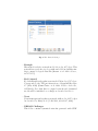
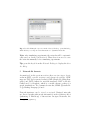
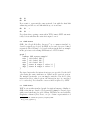
Version 3.1 Beta
October 5, 2012
GeneNetWeaver User Manual
In silico benchmark generation and performance profiling of network inference methods
Thomas Schaffter, Daniel Marbach, Gilles Roulet
GeneNetWeaver User Manual
In silico benchmark generation and performance profiling of network
inference methods
Version 3.1 Beta
October 5, 2012
Thomas Schaffter
Ecole Polytechnique F´ed´erale de Lausanne (EPFL), Laboratory of
Intelligent Systems, Lausanne, Switzerland
Daniel Marbach
MIT Computer Science and Artificial Intelligence Laboratory,
Cambridge, Massachusetts, USA; Broad Institute of MIT and Harvard,
Cambridge, Massachusetts, USA
[email protected]
http://lis.epfl.ch/gnw
Table of Contents
1 Introduction . . . . . . . . . . . . . . . . . . . . . . . . . . . . . . . . . . . . . . . .
4
1.1 Overview . . . . . . . . . . . . . . . . . . . . . . . . . . . . . . . . . . . . . . .
4
1.2 License / how to cite us . . . . . . . . . . . . . . . . . . . . . . . . . .
5
1.3 Using this manual . . . . . . . . . . . . . . . . . . . . . . . . . . . . . . .
5
1.4 How to contact the GNW project . . . . . . . . . . . . . . . . . .
5
2 Getting Started . . . . . . . . . . . . . . . . . . . . . . . . . . . . . . . . . . . . .
6
2.1 Launching GNW . . . . . . . . . . . . . . . . . . . . . . . . . . . . . . . .
6
2.2 Embedded tutorial . . . . . . . . . . . . . . . . . . . . . . . . . . . . . . .
7
3 The Network Desktop . . . . . . . . . . . . . . . . . . . . . . . . . . . . . . . .
7
3.1 Automatically loaded networks . . . . . . . . . . . . . . . . . . . .
7
4 Opening and saving network structures and dynamical models 9
4.1 Opening networks . . . . . . . . . . . . . . . . . . . . . . . . . . . . . . .
9
4.2 Saving networks . . . . . . . . . . . . . . . . . . . . . . . . . . . . . . . . .
9
5 Network file formats . . . . . . . . . . . . . . . . . . . . . . . . . . . . . . . . . 10
5.1 TSV format . . . . . . . . . . . . . . . . . . . . . . . . . . . . . . . . . . . . . 11
5.1.1 Examples. . . . . . . . . . . . . . . . . . . . . . . . . . . . . . . . . . . 11
5.2 GML format . . . . . . . . . . . . . . . . . . . . . . . . . . . . . . . . . . . . 12
5.3 DOT format . . . . . . . . . . . . . . . . . . . . . . . . . . . . . . . . . . . . 12
5.4 SBML format . . . . . . . . . . . . . . . . . . . . . . . . . . . . . . . . . . . 13
6 Visualizing networks . . . . . . . . . . . . . . . . . . . . . . . . . . . . . . . . . 13
7 Extracting subnetworks from a source network . . . . . . . . . . . 16
8 Random initialization of dynamics . . . . . . . . . . . . . . . . . . . . . 18
9 Simulation of experiments . . . . . . . . . . . . . . . . . . . . . . . . . . . . 19
9.1 Description of exported files . . . . . . . . . . . . . . . . . . . . . . . 22
9.1.1 Unsigned network structure / DREAM gold standard. 23
9.1.2 Signed network structure. . . . . . . . . . . . . . . . . . . . . 23
9.1.3 Dynamical network model. . . . . . . . . . . . . . . . . . . . 23
9.1.4 Steady-state datasets. . . . . . . . . . . . . . . . . . . . . . . . . 23
9.1.5 Time series datasets. . . . . . . . . . . . . . . . . . . . . . . . . 24
10 Evaluating network predictions . . . . . . . . . . . . . . . . . . . . . . . . 25
10.1 Precision-Recall and ROC curves . . . . . . . . . . . . . . . . . . 27
10.2 Network Motif Analysis . . . . . . . . . . . . . . . . . . . . . . . . . . 27
10.3 Gold standards and network prediction format . . . . . . . 30
10.4 Generating PDF reports . . . . . . . . . . . . . . . . . . . . . . . . . . 31
10.5 Matlab scripts . . . . . . . . . . . . . . . . . . . . . . . . . . . . . . . . . . . 32
11 Settings/configuration files . . . . . . . . . . . . . . . . . . . . . . . . . . . .
12 Command-line interface and standalone version . . . . . . . . . .
13 Visualization of data in Matlab . . . . . . . . . . . . . . . . . . . . . . . .
14 License . . . . . . . . . . . . . . . . . . . . . . . . . . . . . . . . . . . . . . . . . . . . .
32
32
33
34
1
1.1
Introduction
Overview
Numerous methods have been developed for inference of gene regulatory networks from expression data, however, their strengths and
weaknesses remain poorly understood. Accurate and systematic evaluation of these methods is hampered by the difficulty of constructing
adequate benchmarks and the lack of tools for a differentiated analysis of network predictions on such benchmarks.
GeneNetWeaver (GNW) is an open-source tool for in silico benchmark generation and performance profiling of network inference methods. GNW can be launched directly from any web browser and it has
an intuitive graphical user interface. Using GNW it is possible to
generate biologically plausible in silico gene networks and simulated
expression data, which can be used as benchmarks for network inference methods. Realistic network structures are generated by extracting modules from known biological interaction networks(Marbach et al.
2009). These networks are then endowed with dynamics using a kinetic model of transcription and translation, where transcriptional
regulation is modeled using a thermodynamic approach allowing for
both independent and synergistic interactions. Finally, these models
are used to produce synthetic gene expression data by simulating
different biological experiments. Simulations can be done either deterministically or stochastically to model internal noise in the dynamics of the networks, and experimental noise can be added using
a model of noise observed in microarrays.
Another important feature of GNW is systematic evaluation of the
predictions from different inference methods on in silico networks
in the benchmark. For a set of network predictions from one or several inference methods, GNW automatically generates a comprehensive report in PDF format. These reports include standard metrics
used to assess the accuracy of network inference methods such as
precision-recall and receiver operating characteristic (ROC) curves.
Furthermore, the reports include network motif analysis (Marbach et al.
2010), where the performance of inference methods is profiled on local connectivity patterns. The network motif analysis often reveals
systematic prediction errors, thereby indicating potential ways of
network reconstruction improvements.
We are using GNW to provide an annual network inference challenge
for the DREAM project (Marbach et al. 2010). In the past three
editions, a total of 91 teams submitted over 800 network predictions
to evaluate the performance of their methods on GNW-generated
benchmarks.
You can launch GNW directly from your browser by clicking the
Launch GNW button on the top right of our website (gnw.sf.net). If
it doesn’t work, make sure that you have Java Web Start installed.
1.2
License / how to cite us
GNW is released open-source under an MIT license (see Sect. 14).
If you use GNW for your research, please cite the papers indicated
on our website: gnw.sourceforge.net/publications.html.
1.3
Using this manual
The purpose of this manual is to explain the different functionalities
offered by GNW. The algorithms and models that GNW is based
upon are not explained here. If you intend to use GNW for your
research, we recommend first reading our publications listed on our
website.
1.4
How to contact the GNW project
The GNW project can be contacted via its website (gnw.sf.net).
Please feel free to contact us with bug reports, feature requests, and
information on related projects.
2
Getting Started
2.1
Launching GNW
GNW is ditributed through the Java Web Start technology developed by Sun (see Sect. 12 for information on how to run GNW
from the command-line and as standalone version). This allows any
computer on which Java Web Start is installed to run GNW, independently of the operating system used. GNW requires Java version
1.5 or later.
Launching GNW is as simple as one click! Please visit the GNW
website (gnw.sf.net) from where you will be able to run GNW by
clicking on the Launch GNW button. If it doesn’t work, make sure
that you have Java Web Start installed1 . Java Web Start will download the application and ask whether you trust the LIS Certificate.
You must accept the certificate in order to run GNW.
Fig. 1. Click Allow to accept the LIS Certificate, which allows GNW to work
outside its sandbox.
Next, you may be asked whether you want to install a GNW shortcut
on your Desktop. After that, the main screen of GNW will appear.
According to its default settings, Java Web Start saves all the components needed to run GNW in the cache. This will significantly
reduce loading time compared to the first time that you launched
1
java.sun.com/products/javawebstart
GNW. It also makes it possible to run GNW offline, i.e. without
internet connection If you do have an internet connection, Java Web
Start automatically checks for new versions of GNW.
2.2
Embedded tutorial
Before reading this document, we recommend that you do the short
tutorial that is embedded in GNW. You can access the tutorial by
clicking on the corresponding button on the menu bar of the main
GNW window. The tutorial will guide you through the following
steps (each step is explained more in detail in the present document):
1.
2.
3.
4.
5.
6.
7.
8.
Opening a source network structure
Extracting subnetworks from the source networks
Visualizing the extracted subnetworks
Generating a kinetic model
Generating datasets
Evaluating network predictions
Using configuration files to specify GNW parameters
Using the command-line interface and standalone version of GNW
3
The Network Desktop
At start up, the main window of GNW appears with the Network
Desktop open (see Fig. 2). The Network Desktop can always be accessed through the Desktop button from the menu bar of the main
window. It is dedicated to all the operations related to the networks, e.g., opening networks, generating benchmark networks and
datasets, or visualization and export of networks.
Two types of networks are handled by GNW, which can be distinguished by the color of their icon in the Network Desktop. Network
structures have a blue icon. A network structure is a directed graph,
possibly with signed edges. Dynamical networks have an orange icon.
These are dynamical models of gene networks that can be used to
simulate experiments and generate corresponding datasets.
3.1
Automatically loaded networks
Several network structures and dynamical networks are automatically loaded when GNW is started:
Fig. 2. The Network Desktop
– Example
Hierarchical scale-free network model: 64 nodes, 207 edges. This
network has a scale-free topology with embedded modularity similar to many biological networks (Ravasz et al. 2002. Science,
297:1551-55).
– Ecoli (signed)
E.coli transcriptional regulatory network: 1502 nodes, 3587 edges.
Corresponds to the TF-gene interactions of RegulonDB release
6.7 (May 2010) (Gama-Castro et al. 2008. Nucleic Acids Res,
36:D120-4). Note that this is a signed network and dynamical
models will be initialized accordingly as described in Sect. 8.
– Yeast
Yeast transcriptional regulatory network: 4441 nodes, 12873 edges.
As described by Balaji et al. (J Mol Biol, 360:213-27, 2006).
– DREAM Challenges
This folder contains dynamical networks generated with GNW
and used as gold standards for the DREAM network inference
challenges.
4
Opening and saving network structures and dynamical
models
4.1
Opening networks
To import a network, click the Open icon of the Network Desktop
and use the dialog to browse your folder and open a file. If you click
on the field Files of Type of the Open dialog, a list of the different
network file formats supported by GNW will appear (see Fig. 4.1).
You can open network structures saved in TSV, GML, and DOT format. For dynamical models SBML is used2 . See the next section for
a description of these formats. If the network is successfully parsed,
a new network icon will appear in the Network Desktop.
Tip: press the key O from the Network Desktop to display the Open
dialog.
Tip: press the key RETURN or DELETE from the Network Desktop to delete networks and folders.
Important: the filenames must end with the correct extension, otherwise they are not visible in the Open dialog and GNW will refuse
to load them. The recognized extensions are .tsv, .gml, .dot and .xml
(since SBML is based on XML).
4.2
Saving networks
After having extracted subnetworks, you probably want to save them
for later use. To export networks from GNW, double-click the icon of
the network and select the option Export Network. A dialog appears
that allows you to specify a filename and to select a file format before saving the network. SBML format is only available for dynamical
networks (as mentioned above, the SBML format that GNW uses is
not yet compatible with other simulators).
2
In the current version, only SBML files that have been generated by GNW can be
opened.
Fig. 3. Double-clicking the Open icon in the Network Desktop opens this dialog,
which allows you to import network structures or dynamical networks.
Note: after simulating experiments, the networks will be automatically saved as described in Section 9. Thus, there is no need to save
the networks manually before simulating experiments.
Tip: press the key S from the Network Desktop to display the Save
As dialog.
5
Network file formats
As mentioned in the previous section, there are two types of networks in GNW: network structures and dynamical networks. GNW
supports TSV (tab-separated-values), GML (Graph Modelling Language) and DOT formats for network structures. DOT is the file
format used by Graphviz, which is a useful software package for
graph visualization3 . For dynamical networks, SBML (Systems Biology Markup Language) is used.
Network structures can be signed or unsigned. Unsigned networks
are directed graphs without any information on the regulatory effect
(enhancing or inhibitory) of interactions. In signed networks, the
3
http://www.graphviz.org
regulatory effect of interactions is specified. The type of interaction
is either enhancing (+) or inhibitory (-).
5.1
TSV format
This format is the easiest way to describe a network structure in
GNW. Each line corresponds to a regulatory interaction from a
source node (the regulator) to a target node. A line is composed
of the following elements, separated by a tabulation:
– Source node
– Target node
– Attribute (optional)
Both source and target nodes are represented by an identifier (string),
and the optional attribute is used to specify the type of the interaction. There are two different flavors of the TSV format for signed
and unsigned network structures:
– TSV network structure (*.tsv)
Should be used to save signed network structures. The attribute
is either ‘+’ (enhancing), ‘−’ (inhibitory), ‘+−’ (dual), ‘?’ (unknown), or ‘0’ (zero). Note, if the value for the attribute is omitted, the interaction is assumed to be of type unknown.
– DREAM gold standard network structure (*.tsv)
This is the file format used for the network structures in the
DREAM challenge (the gold standards). The networks are unsigned, thus there is no attribute. Optionally, the attribute may
be set to ‘1’ (present links) or ‘0’ (absent links).
Important: It is usually not necessary to list the absent links (attribute ‘0’) because links that are not listed are automatically assumed to be absent. We allow for the possibility to explicitly list the
absent links for compatibility with the format used in the DREAM
challenge. Also, it allows to add nodes to the network that have no
connection. For example, the line “A A 0” will add the node A with
no connections to the network.
5.1.1
Examples. Consider a network with three nodes G0, G1, G2,
with an interaction from G0 to G1 and from G0 to G2. This network
can be described in TSV format by
G0
G0
G1
G2
If we want to represent the same network, but with the first link
enhancing and the second link inhibitory, we would use
G0
G0
G1
G2
+
-
Note that when opening a network in TSV format, GNW automatically detects whether the network is signed or not.
5.2
GML format
GML, the Graph Modelling Language 4 , is a common standard to
describe network topologies. In GML, nodes and edges are defined
separately. The following code describes the network used as example
in the previous section using GML instead of TSV format.
graph [
comment "GML syntax example"
node [ id 0 label "G0" ]
node [ id 1 label "G1" ]
node [ id 2 label "G2" ]
edge [ source 0 target 1 value "+" ]
edge [ source 0 target 2 value "-" ]
]
For signed networks, the interaction types are specified by the field
value using the same attributes as defined in the previous section.
For unsigned networks, you can simply omit the value field of the
interactions (if no value is given, the interaction type is considered
to be unknown). Note that the comment field is ignored by GNW.
5.3
DOT format
DOT is yet another standard graph description language. Similar to
GML, networks are described by separately defining nodes and edges
with several attributes for each of them. DOT files are used with the
Graphviz5 softwares (Dot, Neato, etc.) to obtain a representation of
4
5
http://www.infosun.fim.uni-passau.de/Graphlet/GML
http://www.graphviz.org
the graph as image (PNG, PDF, EPS, etc.). Only a small part of the
features of the DOT language are used by GNW. The example below
shows the code for the network described in the previous sections,
this time in DOT format
digraph [
"G0";
"G1";
"G2";
"G0" -> "G1" [value="+"];
"G0" -> "G2" [value="-"];
]
The value field is used by GNW as explained in the previous section
for the GML format.
5.4
SBML format
The Systems Biology Markup Language (SBML) is a standard format to represent dynamical models of biological systems. GNW uses
SBML to open/save dynamical networks. For a detailed description
of SBML, please refer to the web site of the SBML project6 .
6
Visualizing networks
GNW has an easy-to-use interface to visualize the networks that you
have imported or generated with the subnetwork extraction method.
The visualization is based on the excellent Java library JUNG (Java
Universal Network/Graph Framework), an open-source project available on SourceForge.net7 . To visualize a network from the Network
Desktop, double-click it and choose Visualization.
Tip: press the key V or use the third/middle button of your mouse
to open the graph visualization window directly from the Network
Desktop.
Warning: visualization is mainly thought for medium or small networks (less than 200 nodes). You can try to visualize larger networks,
6
7
http://www.sbml.org
http://jung.sourceforge.net
Fig. 4. The GNW network visualization interface.
but it may take a long time and the graph layout probably won’t be
be well arranged.
Tip: alternatively, you can export your network in DOT format and
use Graphviz or other professional tools for graph visualization (see
Section 5.3).
Click and drag to move the graph around, and use the scroll wheel
to zoom in our out. Use the link Display help in the visualization
window for information on additional actions (e.g., rotation) that
you can perform on the graph.
The Visualization Controls panel in the left part of the visualization
window allows to change and manipulate the graph representation
in a number of ways:
– Move graph/nodes
In move graph mode, you can move the whole graph using the
left mouse button. In the move nodes mode you can move one
or several nodes, which is useful if the automatic graph layout is
not optimal.
– Graph layouts
Three different layouts allow to change the way the nodes are
distributed:
• Kamada-Kawai algorithm (force-based)
• Fruchterman-Reingold algorithm (force-based)
• Positions vertices equally spaced on a regular circle.
– Vertex search
Searching a specific node in a network with thousands of nodes is
like looking for a needle in a haystack! Vertex search helps you to
find a node or group of nodes according to their labels. If an entered string corresponds exactly to the label of a node, the node
is highlighted red and the search field becomes green. If the entered string partly matches several node labels, these nodes will
appear in orange. If the string matches no label, the search field
will become red.
– Display labels
If checked, the labels of the nodes are displayed.
– Curved edges
If checked, the interactions are represented by curved edges instead of straight lines.
– Distinguish signed edges:
• by arrow head
If checked, signed interactions have different arrow heads depending on their type, as shown in the legend in the bottom
left corner of the visualization window (see Figure 4). If the
network is unsigned, all the interactions are of type unknown.
• by color
If checked, signed interactions are colored as shown in the
legend mentioned above. If the network is unsigned, all the
interactions are of type unknown.
– Export as image
Take a snapshot of the graph. The network can be exported in
JPEG, PNG, and EPS image formats.
7
Extracting subnetworks from a source network
Important: we assume that you have read our paper (Marbach et al.
2009), which describes and motivates the subnetwork extraction method
for generating reverse engineering benchmarks.
Click the Networks button in the main window of GNW to enter the
Network Desktop. Double-click the source network from which you
want to extract subnetworks. Click Subnetwork extraction to open
the subnet extraction dialog, which allows you to set the different
parameters for the extraction. We will now explain each of the fields
of this dialog:
– Subnets name
The prefix of the name of the subnets. If you enter the name subnet, the extracted subnetworks will be named subnet-1, subnet-2,
etc.
– Extract all regulators
Extract all regulators of the networks, i.e. all nodes that have at
least one outgoing link in the source network. E.g. if the source
network is Ecoli, the extracted network would consist of all E.coli
transcription factors.
– Number of subnets
The number of subnetworks that you want to extract.
– Include at least N regulators
Select to specify the minimum number of regulators (nodes that
have at least one outgoing link in the source network ) that should
be included in the extracted subnetworks.
– Seed
• Random vertex
For each subnet, the extraction method starts from a different
randomly picked seed node of the source network.
• Selection from list
Select the seed node manually from the list of all nodes of the
source network.8
• From strongly connected components
Add the specified number of nodes from the largest strongly
connected component of the graph as seeds. Warning: this
works fine if the network has a single strongly connected component, as Yeast does. However, if there are several stongly
connected components, the smaller ones will never be sampled
(to be corrected in the next version).
– Neighbor selection
• Greedy
In the subnetwork extraction process, always choose the neighboring node for addition that maximizes the modularity (if
several neighbors lead to the same modularity, one of them is
chosen randomly).
• Random among top (%)
Specify a percentage p. Instead of always adding the neighboring node that maximizes the modularity, one of the top p%
neighbors with the highest modularity is chosen randomly.
The effect of this parameter is discussed in the methods section of Marbach et al. (2009): varying p between 0% and 100%
allows for tuning of the sampling strategy from pure modular
subnetwork extraction to random subnetwork extraction. We
usually use either the greedy strategy or p = 10% to add some
stochasticity.
Click Extract to run the subnetwork extraction. This may take a
minute for large networks. You can see the order in which neighboring nodes are added to the subnetwork in the console, along with
8
Note, if you extract several subnetworks from the same seed, they are usually very
similar, but not necessarily identical. They are not identical because if in the subnetwork extraction process several neighboring nodes lead to the same modularity,
one of them is chosen randomly.
the modularity at each step.
Tip: press the key E from the Network Dekstop to display the Subnetwork Extraction dialog.
8
Random initialization of dynamics
Click the Networks button in the main window of GNW to enter
the Network Desktop. Double-click the network structure (network
structures have blue icons) that you want to convert into a dynamical
network model. Usually this is a subnetwork that you have previously
extracted as described in the previous section.
Click Random initialization of dynamics. In the dialog, leave the
checkbox checked if you want to remove autoregulatory interactions
(self-loops). Otherwise, uncheck it. If your network has no autoregulatory interactions, this option has no effect.
For the DREAM challenges, we have removed autoregulatory interactions for the following reason. A first class of reverse engineering
methods cannot identify autoregulatory interactions and will consequently set them all to zero per default. A second class of methods
tries to infer autoregulatory interactions, but in our experience this
is quite difficult. Since overall, there are few autoregulatory interactions in the transcriptional networks that we considered, paradoxically the first class of methods would actually perform well: since
they set all autoregulatory interactions to zero, and a large majority
are indeed zero, the performance is actually very good. In contrast,
the methods that try to infer the few autoregulatory interactions
risk to have many false positives. In order not to favor the first or
the second class of methods, we did not ask participants to predict
autoregulatory interactions and removed them from the DREAM
challenge networks.
Important: for signed network structures, the dynamics are initialized such that the signs in the dynamical network are the same as
in the original network structure. In other words, excitatory / inhibitory interactions will be initialized such that they actually have
an excitatory / inhibitory effect in the dynamical model. For un-
signed network structures, the signs in the dynamical model are initialized arbitrarily.
Refer to Marbach et al. (2010) for a description of our modeling approach, a more detailed description of the kinetic model is in preparation. Note that the initialization is done such that the created regulatory dynamics are biologically plausible–we have confirmed that
the kinetic model has excellent agreement with the regulatory dynamics of experimentally mapped promoters in E. coli.
Tip: press the key K to open the dialog to generate kinetic models.
9
Simulation of experiments
Click the Networks button in the main window of GNW to enter
the Network Desktop. Double-click the dynamical model (dynamical
networks have an orange icon) that you want to simulate to produce
datasets. Click Generate datasets. In the dialog that pops up, you
can specify the type of experiments and the amount of noise that
you want to add to the data.
– Model. Select ODEs (deterministic) or SDEs (noise in dynamics) for the simulation of the experiments. If you select both, they
will be run one after the other using the exact same perturbations
(the label nonoise will be added to the data from the ODEs).
– Experiments
• Wild type. The steady-state levels of the wild-type (the unperturbed network).
• Knockouts. Steady-state levels of single-gene knockouts (deletions). An independent knockout is provided for every gene of
the network. A knockout is simulated by setting the transcription rate of this gene to zero.
• Knockdowns. Steady-state levels of single-gene knockdowns.
A knockdown of every gene of the network is simulated. Knockdowns are obtained by reducing the transcription rate of the
corresponding gene by half.
• Multifactorial. Steady-state levels of variations of the network, which are obtained by applying multifactorial perturbations to the original network. Each data line gives the steady
state of a different perturbation experiment, i.e., of a different
variation of the network. One may think of each experiment
as a gene expression profile from a different patient, for example. We simulate multifactorial perturbations by slightly
increasing or decreasing the basal activation of all genes of
the network simultaneously by different random amounts.
• Dual knockouts. Dual knockouts consist of simulating a network with two genes knocked-out simultaneously.
• Timeseries. Time courses showing how the network responds
to a perturbation and how it relaxes upon removal of the
perturbation. The initial condition always corresponds to a
steady-state measurement of the wild-type. At t=0, a perturbation is applied to the network as described below. The
number of time points does not affect the precision of the numerical integration, this is just the number of time points that
will be saved in the dataset.
• Time Series as in DREAM4. If selected, the first half of
the time series shows the response of the network to the perturbation (at t=0 is the wild-type steady-state). Then the
perturbation is removed. The second half of the time series
shows how the gene expression levels go back from the perturbed to the wild-type state.
• Number of time series. The number of time series (a different perturbation is used for every time series).
• Duration of each time serie (t max). Total duration of
each time series experiment.
• Number of measured points per time series. Number
of points per time series (defines how many points are saved
in the datasets, does not affect precision of numerical integration).
• Perturbations for multifactorial, dual knockouts, and
DREAM4 time series
∗ Generate new. Generate new perturbations, select if you
don’t have predefined perturbations that you want to use.
∗ Load from files. Load the perturbations from the following files (they must be located in the output directory):
<networkName> multifactorial perturbations.tsv,
<networkName> dualknockouts perturbations.tsv,
<networkName> dream4 timeseries perturbations.tsv
Please generate a few perturbations with GNW and look at
the corresponding files to understand the format, we intend
to improve how perturbations can be specified by the user in
the next version of GNW and will provide a more detailed
description at this point. In the meantime, please contact us
if you have questions. Note that the file defining the dualknockouts specifies the maximum transcription rate of every gene in the perturbed state—it can in fact be used to
specify arbitrary perturbations of the maximum transcription
rates and not just dual knockouts. The multifactorial and
dream4 timeseries perturbation files specify the amount by
which the basal transcription rate is perturbed for every gene.
– Noise
• Coefficient of noise term. Multiplicative constant of the
noise term in the SDEs (if set to 0, using SDEs is equivalent
to using ODEs).
• Noise added after the simulation (measurement error)
∗ None. No measurement error is added.
∗ Model of noise in microarrays (used in DREAM4).
Select to use the model of noise in microarrays that was
used for the DREAM4 challenges, which is similar to a
mix of normal and log-normal noise (Tu, Stolovitzky, and
Klein. PNAS, 99:14031-14036, 2002).
∗ Add normal and/or log-normal noise. Select to add
normal (Gaussian) and/or log-normal noise after the simulation.
∗ Normalize after adding noise (as in DREAM4). After adding experimental noise (measurement error), normalize by dividing all concentrations values by the maximum mRNA concentration of all datasets.
– Output directory. GNW will automatically save all relevant
files of the benchmark (the simulated datasets, the network structure, the dynamical model of the network, etc.) in the output
directory specified here. See the next section for a description of
the exported files.
After clicking OK, GNW will simulate the experiments and save the
files described in the next section in the specified output directory.
Tip: press the button DREAM4 settings to generate the same type
of experiments as those of the DREAM4 in silico challenge.
Tip: press the key B (for Benchmarks) from the Network Desktop
to directly display the Experiments Simulation dialog (works only
for dynamical models).
9.1
Description of exported files
GNW uses different file types to save network structures, dynamical
network models, and various types of data from simulated experiments. All files except the dynamical network model are saved in
tab separated value format (TSV). These are text files that you
can open and edit with any text editor or Excel, for example. Note
that you can easily convert .tsv format into the sometimes preferred
comma separated value format (CSV) by using the search and replace function of your text editor to replace all tabs with commas.
In the next sections we describe the format of all files that are saved
by GNW automatically after the simulation of experiments.
Unsigned network structure / DREAM gold standard. GNW
saves the unsigned network structure in a file called <name> goldstandard.tsv,
where <name> is the name of the network in the Network Desktop. The file is in TSV format and can subsequently be opened with
GNW as described in Section 4. For each regulatory link from a gene
A to a gene B there is a line “A B 1” in the file.
9.1.1
Note: To save space, we do not list all the zero connections as done
in the DREAM gold standards. Consequently, the evaluation script
to compute the scores of a prediction available from the DREAM
website gives an error. To address this issue, you should either use
the evaluation functionality of GNW (which computes PR and ROC
curves in the same way as the DREAM scripts), use the adapted
version of the DREAM scripts that are available on our website
(gnw.sf.net), or reopen the file with GNW and export it to the format DREAM gold standard network structure (*.tsv), where the zero
connections are explicitly written as described in Section 4.
Signed network structure. The signed network structure is
saved in the file <name> goldstandard signed.tsv. The file can be
opened with GNW as described in Section 4. For each regulatory
link from a gene A to a gene B there is a line “A B <sign>”, where
<sign> is ‘+’ if the interaction is enhancing and ‘-’ if the interaction
is inhibitory. We don’t provide a script to evaluate signed predictions,
but one could use the same approach as in DREAM2.
9.1.2
9.1.3
Dynamical network model. The dynamical network is saved to
the file <name>.xml in Systems Biology Markup Language (SBML)
format. (However, as mentioned above, currently these files can only
be opened with GNW and are not compatible with other SBML
tools).
9.1.4
Steady-state datasets. The wild-type steady-state is saved to
<name> wildtype.tsv. The knockout and the heterozygous knockdown data are saved to the files <name> knockouts.tsv and <name> knockdowns.tsv,
respectively. Each line contains a knockout or knockdown experiment. The columns correspond to the genes, as indicated by the
lables in the header line. These files can be loaded and visualized
in Matlab with the scripts described in Section 13. Mutlifactorial
steady-states are saved to <name> multifactorial.tsv and dual knockouts steady-states to <name> dualknockouts.tsv. If noisy datasets
are produced, GNW saves in addition the data before addition of
noise in separate files with the prefix nonoise (ODE model, no measurement noise) and noexpnoise (SDE model, no measurement noise).
Furthermore, the protein concentrations with and without noise are
also saved in corresponding files with the prefix proteins.
Note: Perturbations applied to multifactorial and dual-knockout
experiments are saved to <name> multifactorial perturbations.tsv
and <name> dualknockout perturbations.tsv, where each line corresponds to a different perturbation experiment. Please generate a few
perturbations with GNW and look at the corresponding files to understand the format, we intend to improve how perturbations can be
specified by the user in the next version of GNW and will provide
a more detailed description at this point. In the meantime, please
contact us if you have questions. Note that the file defining the dualknockouts specifies the maximum transcription rate of every gene in
the perturbed state. The multifactorial and dream4 timeseries perturbation files specify the amount by which the basal transcription
rate is perturbed for every gene. For example, a value of 0.5 means
that the basal transcription rate of that gene was increased by 0.5.
A value of zero means that this gene was not directly perturbed
(it may have been indirectly perturbed due to perturbations of its
regulators). In addition, the files <name> dualknockouts indexes.tsv
contain the indexes of the genes that were knockouted out in each
dual knockout experiment.
9.1.5
Time series datasets. Time series are saved to files <name> <type> timeseries.tsv,
where <type> is the type of time series experiment (knockout, knockdown, dualknockout, multifactorial, or dream4, as described in Sect.
9). Each line corresponds to a time point, the time is given in the
first column. The following columns correspond to the genes as indicated in the header line. If several time series were produced, they
are saved in the same file one after the other, separated by an empty
line. In the trajectories from wild-type to knockout/knockdown, the
k’th time series corresponds to the knockout/knockdown of gene k.
As for the steady-state experiments, if noisy datasets are produced,
GNW saves in addition the data before addition of noise in separate
files with the prefix nonoise (ODE model, no measurement noise)
and noexpnoise (SDE model, no measurement noise), and the protein concentrations with and without noise are saved in the files with
the prefix proteins.
Note: The applied perturbations described in the previous subsection are saved to the files:
<name> dualknockouts timeseries perturbations.tsv
<name> dualknockouts timeseries indexes.tsv
<name> multifactorial timeseries perturbations.tsv
10
Evaluating network predictions
Use the Evaluation panel to evaluate the predictions of one or several
inference methods using precision-recall and ROC curves (Sect. 10.1)
and/or network motif analysis (Sect. 10.2). All results are saved in
a text file (XML format) and optionally also in a PDF report that
includes graphical plots (see Sect. 10.4). For either type of analysis,
you first have to specify the gold standards and the network predictions (file formats are described in Sect. 10.3).
First, specify a gold standard using the corresponding drop-down
menu (gold standards must be previously loaded on the Network
desktop). Use the ‘+’ button to add lines if you are evaluating predictions for several gold standards. Next, click Browse to select the
folder where the network predictions are located (this folder is recursively searched for prediction files). GNW tries to automatically
match predictions to gold standards based on similarity of the corresponding file names. If the automatic matching doesn’t work, select
the predictions manually using the drop-down menus. You may also
specify a name for the inference method by double-clicking the title
of the tab (named InferenceMethod1 by default). If you are evaluating several inference methods, create a new tab or duplicate existing
tabs by clicking on the corresponding icons next to the tab titles on
Fig. 5. The Evaluation panel allows to evaluate the predictions of one or several
network inference methods (here ARACNEand CLR algorithms). Note that evaluations can be run to assess the performance of inference methods of different
network types (gene networks, neural networks, etc.).
top.
Important: Create a separate tab for each inference method that
is being evaluated.
Note: Precision-recall and ROC curves will be computed for every
gold standard individually, whereas the network motif analysis is
performed over all gold standards together.
10.1
Precision-Recall and ROC curves
Precision-Recall (PR) and Receiver Operator Characteristic (ROC)
curves are widely used to assess the performance of binary decision
algorithms. Since inferring the structure of a network is a matter of
deciding for each possible interaction if it is present or not, PR and
ROC curves can be used to assess the performance of network reverse engineering algorithms. In the DREAM challenges, algorithms
are assessed based on the area under the PR and ROC curves (AUPR
and AUROC) (Prill et al. 2008). PR and ROC are closely related, see
Davis and Goadrich (2006) for a good discussion. Select the corresponding checkboxes in the Evaluation panel to compute the AUPR
and AUROC, and to plot the curves in the PDF report (see Sect.
10.4 and Fig. 6).
Note: The code for computing the AUPR and AUROC is based on
the DREAM evaluation scripts available from the DREAM website,
which were developed by Robert Prill and Gustavo Stolovitzky.
10.2
Network Motif Analysis
We have developed a methodology to evaluate the performance of
inference methods based on local connectivity patterns (network motifs) and reveal different types of systematic prediction errors. Select
the corresponding checkbox in the Evaluation panel to perform the
network motif analysis as described in our paper (Marbach et al.
2010). The results of this analysis are saved for all three-node motifs in text format in the XML file that is produced when running
the evaluation, and they are visually represented in the PDF report
for a subset of the motifs (fan-in, fan-out, cascade, and feed-forward
loop; see Fig. 7). The XML file contains for every motif and edge
0. 5
1
1
0. 5
0
AU PR = 0.213
0. 5
1
1
0. 5
0
0. 5
1
0. 5
0
0. 5
R ecall
R ecall
R ecall
R ecall
R ecall
AU R OC = 0.801
AU R OC = 0.833
AU R OC = 0.842
AU R OC = 0.759
0. 5
F als e Pos itive R ate
1
0
0. 5
F als e Pos itive R ate
1
0. 5
0
0. 5
F als e Pos itive R ate
1
0. 5
0
1
1
T rue Pos itive R ate
0. 5
1
T rue Pos itive R ate
0. 5
1
T rue Pos itive R ate
1
T rue Pos itive R ate
T rue Pos itive R ate
0. 5
A 5 in s ilic o _s iz e100_5
AU PR = 0.349
1
AU R OC = 0.914
1
0
0. 5
0
A 4 in s ilic o _s iz e100_4
AU PR = 0.39
1
Precis ion
Precis ion
Precis ion
0. 5
0
A 3 in s ilic o _s iz e100_3
AU PR = 0.377
1
Precis ion
A 2 in s ilic o _s iz e100_2
AU PR = 0.536
Precis ion
A 1 in s ilic o _s iz e100_1
1
0. 5
F als e Pos itive R ate
1
0. 5
0
0. 5
1
F als e Pos itive R ate
Fig. 6. Precision-Recall (PR) and Receiver Operator Characteristic (ROC)
curves of network predictions for five gold standards. AUPR and AUROC (area
under the curve) values are shown above the plots.
type the median prediction confidence, the background prediction
confidence, the divergence of the motif from the background prediction confidence, and the p-value indicating the significance of the
divergence (refer to the supplementary information of Marbach et al.
(2010) for a detailed description).
In the XML file, motif and edge types are identified using the id
attribute. Each motif has three nodes, defined as node 1, 2, and 3
as shown in Fig. 7. The six possible types of edges have the following IDs: 1→2 (0), 1→3 (1), 2→1 (2), 2→3 (3), 3→1 (4), and 3→2
(5). There are 13 possible three-node motifs without autoregulatory
loops, the most common ones have the following IDs: fan-out (0),
fan-in (1), cascade (2), and feed-forward loop (6). A complete list is
given in Table 1.
The parameters Max value on color scale, Significance level, and
Bonferroni correction only affect the visualization of the motifs in
the PDF report, they do not affect the numerical values in the XML
file. Max value on color scale defines the range of the color scales (red
and blue color scales in Fig. 7—in this example the max value is 0.3).
You may have to adjust this value to best visualize the prediction
errors of the evaluated methods. Significance level defines the critical p-value, prediction errors with a p-value above this threshold will
Motif prediction confidence
InferenceMethod1
1
1
F a n-out
T rue s tructure
2
3
2
1
F a n-in
1
3
C a s ca de
2
3
2
1
2
3
1
3
2
1
3
1
FFL
Median predic tion
c onfidenc e
2
3
2
3
≤0.5
0.75
1.0
E dge
B ackground prediction confidence
1
2
1
2
S ys tematic prediction errors
InferenceMethod1
1
1
F a n-out
T rue s tructure
2
3
2
1
F a n-in
1
3
C a s ca de
2
3
2
1
2
3
Deviation of motif from
bac k ground predic tion
c onfidenc e
1
3
2
0
0.15
≥ 0.3
0
-0.15
≤ -0.3
3
Fals e pos itives
1
1
FFL
Fals e negatives
2
3
2
3
Not s tatis tic ally
s ignific ant
Fig. 7. Network motif analysis for an inference method that has a pronounced
cascade error (red arrow in the second-last row). Refer to the supplementary
information of our paper for a detailed description of these plots (Marbach et al.
2010).
Table 1. Definition of motif types. The binary strings indicates which edges are
present in each motif type, the order of the edges is (from left to right): 1→2,
1→3, 2→1, 2→3, 3→1, and 3→2 (cf. Fig. 7).
ID
0
1
2
3
4
5
6
7
8
9
10
11
12
Edges
110000
001010
100100
010110
010011
111010
110100
100110
110101
001111
110110
111011
111111
Name
Fan-out
Fan-in
Cascade
−
−
−
Feed-forward loop
Loop
−
−
−
−
Fully connected
be drawn as dashed arrows in the plots. If Bonferroni correction is
checked, the p-values are required to be K times smaller than the significance level, where K is the number of statistical tests performed
(multiple hypothesis testing). If the motif analysis is performed for
a single inference method, K = 18 (fan-in and fan-out have both
3 types of edges because they are symmetrical, cascade and feedforward loop have both 6 types of edges).
For our analysis, we typically used stringent significance levels (0.01)
and Bonferroni correction to focus only on highly significant prediction errors. Note that some prediction errors (especially the less
significant ones) may also be due to various biases arising from the
data or the network structure (e.g., overlapping motifs, which are
not corrected for in this analysis).
10.3
Gold standards and network prediction format
The gold standard file must be formatted as follows:
G0
G0
...
G1
...
G1
G2
1
1
G0
0
Each line defines an interaction oriented from the first gene to the
second gene. The third element is 1 if the interaction is present in
the gold standard and 0 otherwise. Instead of listing the absent (0)
interactions, they can also simply be omitted (see also Sect. 5.1).
The format for the predictions is the same as used for the DREAM
challenges:
G0
G0
...
G1
...
G1
G2
0.98
0.8
G0
0
As in the gold standard file, each line defines an interaction oriented
from the first to the second gene. For each interaction, a confidence
level between 0 and 1 is given that indicates the degree of belief
that the interaction is included in the gold standard. The predictions must be listed in descending order relative to their confidence
level (the first prediction in the list being the most confident). The
confidence levels are only used to verify that the list of predictions is
correctly ordered, they do not affect the PR and ROC curves and the
motif analysis in any other way. See the DREAM website9 for additional information. Marbach et al. (2008) discuss different strategies
for deriving confidence levels from standard network predictions.
10.4
Generating PDF reports
Evaluation results are always saved in a text file (XML format).
In addition, GNW can generate PDF reports with plots from these
data (an internet connection is required). Check the option Generate
PDF report and fill in the (optional) fields Author, Report ID and
Notes for any additional information you would like to appear on
the report.
Click on Generate to run the evaluation and create the report. If
you don’t have an internet connection, you can still run the evaluation but no PDF report will be created. A PDF report can then be
9
http://wiki.c2b2.columbia.edu/dream/index.php/The DREAM3 In-SilicoNetwork Challenges. Description
generated later from the saved XML file using the button Generate
from source.
10.5
Matlab scripts
On our website (gnw.sf.net) we provide a modified version of the
Matlab evaluation script of the DREAM3 and DREAM4 challenges
(written by G.A. Stolovitzky, B. Jagla, and R. Prill). The file is
called evaluation.m and can be used to plot the PR / ROC curves
and compute AUPR / AUROC scores. The script takes as input a
gold standard file, a prediction file, and the size of the network. Type
help evaluation in Matlab for further information.
11
Settings/configuration files
All parameters that can be specified using the Graphical User Interface (GUI) can also be defined in a settings file. The advantage of
using a settings file is that it can be saved together with a benchmark. Later, it’s easy to verify which parameter values have been
used to generate that benchmark or to generate additional benchmarks of the same type.
Settings files can be loaded from the GUI. It’s also possible to load
a settings file automatically at startup of GNW by naming it settings.txt and placing it in the folder gnw/ of the user’s home directory. For the most common platforms the file should be located
in:
– Windows C:\Documents and Settings\user name\gnw\settings.txt
– Mac /Users/user name/gnw/settings.txt
– Linux /home/user name/gnw/settings.txt
Settings files can be edited and saved from the GUI or using any
text editor. After loading a settings file, the loaded parameter values
will be used as default values in all dialogs.
12
Command-line interface and standalone version
Since version 3.0, it is possible to run GNW using command line
arguments directly from the console or terminal. First, download
the standalone version of GNW from the project website. Then place
yourself in the same directory as gnw-standalone.jar and execute the
following command to display the help menu:
$ java -jar gnw-standalone.jar --help
The help menu lists and describes all command-line arguments. In
addition, the help displays examples of commands to:
–
–
–
–
–
Extract subnetworks from a source network
Generate kinetic models
Generate datasets
Evaluate network predictions
Convert networks (between TSV, DOT, GML, and SBML formats)
Note: The specification of a GNW settings file (see Sect. 11) is required for most operations. A default settings file can be downloaded
from the GNW website.
Tip: Use scripts (Bash, Python, etc.) to execute several of the abovementioned tasks and fully automate the generation of networks and
datasets.
It is also possible to run a standalone version of GNW with the GUI:
$ java -jar gnw-standalone.jar
$ java -jar gnw-standalone.jar -c settings.txt
Note: Unlike the Java WebStart version, the standalone version cannot update itself automatically when a new version of GNW is released.
13
Visualization of data in Matlab
We provide two m-files that can be used to load and visualize the
steady-state and time series datasets in Matlab (available for download on gnw.sf.net):
– dream4ss.m is the script for the steady-state data (dream3ss.m
is also provided for DREAM3 datasets). It loads and plots the
null-mutant and heterozygous knockdown steady-state data produced by GNW using the Matlab function clustergram (see Fig.
13). Check the Matlab documentation for clustergram or type
help dream4ss for more information.
– dream3ts.m is the script for the time series data (compatible
with DREAM4). It loads and plots the time series data produced
by GNW. Each time series is plotted in a separate figure. The
profiles of the genes are clustered into groups as shown in Fig.
13. In Matlab, type help dream3ts for more information.
14
License
Copyright (c) 2007-2010, Thomas Schaffter and Daniel Marbach
Permission is hereby granted, free of charge, to any person obtaining a copy of this software and associated documentation files (the
“Software”), to deal in the Software without restriction, including
without limitation the rights to use, copy, modify, merge, publish,
distribute, sublicense, and/or sell copies of the Software, and to permit persons to whom the Software is furnished to do so, subject to
the following conditions:
The above copyright notice and this permission notice shall be included in all copies or substantial portions of the Software.
THE SOFTWARE IS PROVIDED “AS IS”, WITHOUT WARRANTY
OF ANY KIND, EXPRESS OR IMPLIED, INCLUDING BUT NOT
LIMITED TO THE WARRANTIES OF MERCHANTABILITY,
FITNESS FOR A PARTICULAR PURPOSE AND NONINFRINGEMENT. IN NO EVENT SHALL THE AUTHORS OR COPYRIGHT
HOLDERS BE LIABLE FOR ANY CLAIM, DAMAGES OR OTHER
LIABILITY, WHETHER IN AN ACTION OF CONTRACT, TORT
OR OTHERWISE, ARISING FROM, OUT OF OR IN CONNECTION WITH THE SOFTWARE OR THE USE OR OTHER DEALINGS IN THE SOFTWARE.
G2
G10
G8
G9
G5
G7
1
G4
0.8
G6
G3
0.6
0.4
0.2
G1
wt G1
G2
G3
G4
G5
G6
G7
G8
G9
G10
G10
G4
G6
G3
G1
G8
G5
0.5
G9
0
G7
5
G2
wt G1
G2
G3
G4
G5
G6
G7
G8
G9
G10
Fig. 8. Plotting the noisefree steady-state data from the network Ecoli1 of the
DREAM3 challenge of size 10 with dream3ss. On the top, the steady-state concentrations are shown. Values are normalized, thus concentrations range from 0
to 1 (see color bar on the right). Each row corresponds to a gene, and each column
corresponds to an experiment. The first column is the wild-type steady-state.
Then comes, for every gene, first the null-mutant and then the heterozygous
knock-down experiment. The rows are clustered so that genes that have a similar expression pattern across the experiments are grouped together. For example,
you can see that G2, G10, G8, and G9 (the top four rows) are constitutively active and have no inputs. In the second plot, the difference to the wild-type is
shown. Most squares are black, i.e., there is no difference to the wild-type. But
you can see for example that if G10 is knocked out G7 is upregulated (red square
in the bottom right corner), suggesting an inhibitory interaction from G10 to
G7. You can also confirm this in the plot on the top (note that the order of the
rows is different in the two plots).
1
1
1
0.8
0.8
0.8
0.6
0.6
0.6
0.4
0.4
0.4
0.2
0.2
0.2
0
0
0
100
200
0
100
200
0
1
1
1
0.8
0.8
0.8
0.6
0.6
0.6
0.4
0.4
0.4
0.2
0.2
0.2
0
0
100
200
0
0
100
200
0
0
100
200
0
100
200
Fig. 9. Plotting one of the time series without noise from the network Yeast3
of the DREAM3 challenge of size 50 with dream3ts. The colored lines are the
trajectories of the 50 genes, grouped into 6 clusters. The y-axis is the normalized
mRNA concentration and the x-axis is time.
Bibliography
Davis, J., and Goadrich, M. (2006) The Relationship Between Precision-Recall and
ROC Curves. Proceedings of the 23rd international conference on Machine learning,
233-240, 2006.
Marbach, D., Mattiussi, C., and Floreano, D. (2008) Combining Multiple Results of
a Reverse Engineering Algorithm: Application to the DREAM Five Gene Network
Challenge. Annals of the New York Academy of Sciences, 1158:102-113, 2009.
Marbach, D., Schaffter, T., Mattiussi, C., and Floreano, D. (2009) Generating Realistic in silico Gene Networks for Performance Assessment of Reverse Engineering
Methods. Journal of Computational Biology, 16(2) pp. 229-239.
Marbach, D., Prill, R.J., Schaffter, T., Mattiussi, C., Floreano, D. and Stolovitzky, G.
(2010) Revealing strengths and weaknesses of methods for gene network inference.
Proceedings of the National Academy of Sciences, 107(14) pp. 62866291.
Prill, R.J., Marbach, D., Saez-Rodriguez, J., Sorger, P.K., Alexopoulos, L.G., Xue, X.,
Clarke, N.D., Altan-Bonnet, G., and Stolovitzky, G. (2008) Towards a rigorous assessment of systems biology models: the DREAM3 challenges. PLoS One, 5(2):e9202.
Milo, R., Shen-Orr, S., Itzkovitz, S., Kashtan, N., Chklovskii, D., and Alon, U. (2002)
Network motifs: simple building blocks of complex networks. Science 298:824827.
Shen-Orr, S., Milo, R., Mangan, S., Alon, U. (2002) Network motifs in the transcriptional regulation network of Escherichia coli. Nat Genet 31:6468.