Download User Manual for GNLab - The University of Sydney

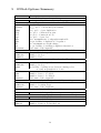
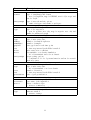
User Manual for GNLab
Joshua W.K. Ho 1,3 and Michael A. Charleston 2,3∗
1
School of Biological Sciences, and
School of Information Technologies,
University of Sydney, Sydney, Australia,
3
Sydney University Biological Informatics and Technologies Centre,
Sydney, Australia
2
January 17, 2007
∗
Correspondent author: M.A. Charleston([email protected])
1
Contents
1 Introduction
1
2 Network Generation
2.1 Modeling evolution of GRNs . . . . . . . . . . . . . . . . . . . . . . . . . .
2.2 Generating Networks with GNLab . . . . . . . . . . . . . . . . . . . . . . .
1
3
3
3 Simulation of Gene Expression Dynamics
3.1 Microarray Dataset Synthesis . . . . . . . . .
3.1.1 Time-series Microarray Dataset . . . .
3.1.2 Gene Perturbation Microarray Dataset
3.1.3 Condition-specific Microarray Dataset
3.2 Experimental Noise Model . . . . . . . . . . .
3.3 Invoking Microarray Simulation in GNLab .
.
.
.
.
.
.
4
5
5
6
6
6
7
4 Network Analysis
4.1 Topological Features . . . . . . . . . . . . . . . . . . . . . . . . . . . . . .
7
7
5 Robustness Score
9
6 Network Visualization
9
7 Network Inference
9
8 Network Comparison
9
9 GNLab Options Summary
.
.
.
.
.
.
.
.
.
.
.
.
.
.
.
.
.
.
.
.
.
.
.
.
.
.
.
.
.
.
.
.
.
.
.
.
.
.
.
.
.
.
.
.
.
.
.
.
.
.
.
.
.
.
.
.
.
.
.
.
.
.
.
.
.
.
.
.
.
.
.
.
.
.
.
.
.
.
.
.
.
.
.
.
.
.
.
.
.
.
11
1
Introduction
GNLab (stand for Gene Network virtual Laboratory) implements a computational
pipeline for large-scale analysis of gene networks. The pipeline allows iterative experiments on GRNs to be designed and carried out in a simple and flexible manner. This
framework consists of distinct functional components for network generation, simulation,
analysis, visualization, inference and comparison. By piping different components together
in different ways, many types of systems biology analyses can be carried out effectively.
Although the development of such a computational pipeline was inspired to assess limitations of GRN inference methods, this pipeline is designed for the general analysis of GRN
structures and dynamics.
Analogous to running various experiments in a laboratory using a range of equipments,
GNLab provides a collection of computational tools that can be used for constructing
various repeatable experiments. The design principle of GNLab is that each functional
component is invoked and controlled separately in a coherent manner. Instead of generating, analyzing and simulating a gene network in a single run, GNLab is invoked
several times and piped together by a simple user-defined script (e.g. using any scripting
language such as Perl or Python). Simple tab-delimited text files are used for communication between each component. GNLab is implemented in ASCII C++, and has a
command-line interface. Individual components of GNLab are invoked by command-line
options. For example, the command GNLab -a net1 reads in a text file net1.gnl.txt
and outputs a detailed summary of topological features in a file called net1.ana.txt. The
command line option -a specifies the action, and any parameters following this option are
the arguments of the call. A list of GNLab command options can be found in Table 1.
The first few sections of this manual explains the theoretical background of most of
tools, and the detailed usage of each option is explained in section 9.
2
Network Generation
A number of procedures have been suggested to generate networks that are topologically
similar to real GRNs. Current algorithms for generating GRNs are mostly mathematically
motivated. Since most biological networks exhibit both small-world (Watts and Strogatz,
1998) and scale-free (Barab´asi and Albert, 1999; Albert and Barabasi, 2000) topology, a
preferential attachment growth model has been used to generate artificial GRNs (Mendes
et al., 2003). An alternative approach is to generate a GRN by sampling a subset of genes
and interactions from experimentally validated gene networks (Van den Bulcke et al.,
2006). Despite being able to generate GRNs of the desired topology, the success of this
method depends on the validity of the source network. None of these can effectively
produce network structures that are topologically consistent with real GRNs.
1
2.1
Modeling evolution of GRNs
To overcome the shortcomings of the existing approaches, a biologically motivated GRN
evolution model, comprising horizontal gene transfer, gene duplication and gene mutation, is proposed. The model is referred to as the Charleston-Ho (CH) model (Ho and
Charleston, in prep.). The CH model is probabilistic in nature. Starting with a small
‘seed network’, a network is grown by iteratively performing one of the evolutionary operators according to their respective probability. The growth process based on this CH
model is governed by a set of ten parameters Table 2.
2.2
Generating Networks with GNLab
The two other commonly used network growth models are the Erd¨os-R´enyi (ER) model (Erd¨os
and R´enyi, 1959), and the Scale-free (SF) model (Barab´asi and Albert, 1999). Networks
generated by these two models have been used as benchmark datasets for evaluating performance of GRN inference methods (Mendes et al., 2003). Along with the CH model,
these two growth models are also implemented in GNLab. To construct a ER network
with n nodes, the model specifies that each of the e edges is randomly inserted between
a pair of nodes. The generation of a SF network relies on two parameters – the number
of nodes (n) and the probability of random edge addition (pAdd ). In the Scale-free model,
either a node insertion or an edge addition event is performed in any one iteration. In
Option Description
Network Generation
-g
Generate a random Charleston-Ho network
-r
Generate a random Erd¨os-R´enyi network
-f
Generate a random Scale-free network
-u
Add or remove a number of edges randomly
-w
Produce a null-model network with the same degree distribution
Network Analysis and Visualization
-a
Calculate network topological features
-n
A produce a one-line summary of topological features
-b
Calculate robustness score
-v
Generate input files for GraphViz, GEOMI, Cytoscape or Pajek
-p
Process a network (e.g. remove activation or repression)
Network Simulation
-s
Simulate microarray data
-t
Generate time-series expression data
Network Comparison
-c
Calculate network topological differences
Others
-d
Convert microarray data into ARACNe and Banjo input files
-e
Provide a seed number for the random number generator
Table 1: Summary of command line options of GNLab.
2
Parameter
n
ptrans
pdup
pig
pil
pgl
mts
pdr
mc
pr
Description
number of genes
probability of horizontal gene transfer
probability of gene duplication
probability of interaction gain
probability of interaction loss
probability of gene loss
maximum size of subgraph transferable
probability of duplication of regulator
maximum arc weight change
probability of retaining a duplicate interaction
Table 2: Description of parameters for the Charleston-Ho model.
a node insertion event, the new node is inserted and linked preferentially to a highly
connected node. In an edge addition event, an edge is randomly added between a pair of
nodes which are preferentially highly connected.
In GNLab, command-line options -r, -f and -g are used to invoke the generation of
random networks using the ER, SF and CH model respectively. The randomly generated
network is written into a simple text file with extension .gnl.txt. This text file contains
information about nodes, edges and edge weights.
3
Simulation of Gene Expression Dynamics
The realistic simulation of the dynamic behaviour of an GRN is essential for simulation
of microarray datasets. Since microarray technology measures gene expression by the
amount of mRNA present, most modeling effect centred around the cellular mRNA level.
The level of mRNA molecules of a gene depends on two processes, namely its synthesis
from gene transcription and its natural breakdown. The level of mRNA synthesis is influenced by the mRNA level of other genes as described by the Hill’s kinetics (Hill, 1910;
Hofmeyr and Cornish-Bowden, 1997). Hill’s kinetics is a non-linear model of gene-to-gene
relationships. It assumes the effect of all regulator genes to the target gene to be multiplicative. Using the same model proposed by Mendes et al. (2003), the dynamics of the
GRN is modeled by a set of ordinary differential equations (ODEs) . Assume that X(Gi )
represents the level of mRNA of gene Gi , and it is activated by genes Ga1 , Ga2 , ..., Gam
and repressed by genes Gr1 , Gr2 , ..., Grn . Constants Kai and Krj represent the expression
levels of Gai and Grj respectively at which the effect on the target gene is half of its
saturating value. The Hill’s constant n controls the sigmoidicity of the interaction curve.
Vi represents the basal transcriptional rate of gene Gi . The rate law for mRNA synthesis
can therefore be formulated as:
n
Y
Krnj
X(Gai )n
)·
(1 +
syn(Gi ) = Vi ·
X(Gai )n + Kani j=1 X(Grj )n + Krnj
i=1
m
Y
3
(1)
The rate mRNA degradation is assumed to only depend linearly on the current expression level. Therefore, the rate law of mRNA breakdown can be formulated as:
break(Gi ) = bi · X(Gi )
(2)
Overall, the change of gene expression level for a gene Gi can be modeled by the
following ordinary differential equation:
dGi
= syn(Gi ) − break(Gi )
(3)
dt
This is a deterministic approach to simulate a GRN. This ODE approach, however,
ignores the inherent stochasticity in the a real gene network. Moreover, solving a large
set of ODEs analytically is computationally intensive, which often requires the use of
approximation methods. In this study, Euler’s method is used to simulate the GRN due
to its simplicity. With the use of a small time-step (e.g. 0.1), Euler’s method is sufficient
to simulate the gene system.
To incorporate stochasticity into the simulation, the deterministic model is extended
into a stochastic model using an approach recently described by Tian and Burrage (2006).
The key is to replace each state variable x in equation 3 by a Poisson random variate with
mean x. The expression of a gene Gi (measured in mRNA molecular number) is simulated
as:
X(Gi , t + τ ) = X(Gi) + P (syn(Gi )) − P (break(Gi ))
(4)
The variable X(Gi , t) denotes the molecular number of mRNA of Gi , and τ denotes
the time elapsed. P (x) generates a Poisson random variate with mean x. Using this
technique, the level of mRNA of a gene is affected by Poisson noise, which is consistent
with the chance event in transcription and translation (Thattai and van Oudenaarden,
2001).
3.1
Microarray Dataset Synthesis
There are three main types of microarray datasets available, namely time-series, gene
perturbation, and condition-specific datasets. A summary of how each type of dataset is
generated is shown as follows:
3.1.1
Time-series Microarray Dataset
1. Initialize the gene system, and simulate 1000×τ rounds to bring the system to a
steady state
2. Knockout one gene (i.e. set concentration = 0, and V = 0)
3. Simulate the system, and repeatedly take the expression level at certain intervals
4
3.1.2
Gene Perturbation Microarray Dataset
1. Initialize the gene system, and simulate 1,000×τ rounds
2. Knockout one gene (i.e. set concentration=0, and V=0)
3. Repeatedly, simulate the system for 1,000×τ rounds
4. Obtain gene expression level after each iteration
3.1.3
Condition-specific Microarray Dataset
1. Initialize the gene system, and simulate 1,000×τ rounds
2. randomly select a set of n genes, each gene is randomly assigned to undertake one
of the following actions:
• conc=0, V=0 (i.e. down regulate)
• conc=conc*2 and V=V*4 (i.e. up regulate)
3. Repeatedly, simulate the system 1,000×τ rounds
4. Obtain the gene expression level after each iteration
3.2
Experimental Noise Model
Microarray is an inherently noisy technology. Being able to incorporate a realistic amount
of noise into the simulated microarray data is essential for a range of microarray analysis
experiments. By studying the structure of microarray noise at the DNA hybridization
and the preparation level, the noise in an oligonucleotide microarray has been shown to
be signal intensity dependent (Tu et al., 2002). In general, the stronger the signal, the less
the signal is affected by noise. In this work, a normal distribution of noise with standard
˙ is applied to each signal with log intensity θ. The term β is the noise
deviation of β e−|θ|
coefficient, which can be varied. The higher the β, the more ‘noisy’ the data becomes.
3.3
Invoking Microarray Simulation in GNLab
In GNLab, network simulation can be carried out using option -t, which generates a
time-series of gene expression. Simulation results are written into a .data file. Timeseries, gene perturbation, and condition-specific microarray datasets can be simulated
from a network using the option -s. The number of technical and biological replicates can
be specified as arguments. The resulting data resemble the microarray data generated by a
one-channel oligonucleotide array. The microarray data can optionally be log-transformed
and mean normalized per array. The microarray data is stored in a .ma.txt file.
5
4
4.1
Network Analysis
Topological Features
A set of 11 commonly used topological features are calculated to characterize a GRN in
GNLab (see Table 3). These features are used to describe the global and local network
properties. For global network statistics, one can extract the number of gene (n), number
of interactions per genes (inter), proportion of genes with self-loops (loop), proportion of
regulator genes (reg), number of disjoint network components (comp), proportion of the
maximum component size (mcs), longest path length (lpl; longest directed path between
a regulator and any other gene), proportion of activation amongst all interactions (act)
and hub dominance (hubDom; defined as the proportion of arcs connected to the top 5%
of most connected genes compared to the total number of arcs). For local properties,
they can be characterized by the average clustering coefficient (cc) and the number of
feed-forward loops per gene (ffl).
In particular, hub dominance is a new topological feature used in GNLab. Normally,
the importance of hub genes is characterized by the slope of a power-law curve. However,
fitting a power-law curve to the out-degree of a GRN may not be appropriate, thus a
new method of measuring hub usage is needed. The idea of measuring the proportion
of arcs connected to the top 5% of hub genes compared to the total number of arcs was
used by Basso et al. (2005). This work formally adopts this measurement as a topological
feature for network analysis.
Topological features can be calculated using option -a, which calculates a range of
topological features such as degree distribution, clustering coefficient distribution, length
of longest path. The results are stored into a file with an .ana.txt extension. The
command-line option -n can be used to print a one-line summary of the 11 topological
features onto the console display. The analysis results from the file can easily be parsed
into statistical analysis packages such as R (Ihaka and Gentleman, 1996).
5
Robustness Score
The dynamic behaviour of a GRN can also be measured by a novel robustness score
devised in this studied. The network robustness can be estimated by the ability of a
network to tolerate random gene perturbation using an in silico simulation procedure. To
calculate the robustness score, a set of k genes is initially labeled as essential genes. One
thousand rounds of simulations are initially performed to bring the system to its steady
state. Then, k mutant genomes are created by systematically knocking out one gene per
mutant genome (i.e. set X(Gi ) = 0) and V (Gi ) = 0). Each mutant genome is further
simulated for 1,000 iterations. If the expression of any essential gene in a mutant genome
is dropped by more than 50%, the mutant is non-viable. The robustness score is the
proportion of viable mutant genomes over all possible single gene mutants. In GNLab,
6
Feature
n
inter
loop
reg
comp
msc
lpl
7
cc
act
hubDom
ffl
Description
number of nodes.
average number of interactions per node.
proportion of nodes with self-loop (e.g. A−→A).
proportion of regulator genes (i.e. nodes with out-degree ≥ 1).
number of disjoint network components.
proportion of the maximum component size.
longest path length. It represents the longest directed path between a regulator and any
other gene. An lpl of one means any regulator in the network can at most influence the
expression of one other gene.
average clustering coefficient. A high clustering coefficient signifies a high local edge density,
and therefore a dense local gene regulation.
proportion of activation amongst all interactions. E.g. if act is greater than 0.5, than
activation is a more important type of regulation compared to repression.
hub dominance, which is defined as the proportion of arcs connected to the top 5% of most
connected genes compared to the total number of arcs. The higher the hub dominance, the
more important the hub genes are.
number of feed-forward loops per gene.
Table 3: Descriptions of the 11 topological features used in GNLab.
robustness scores can be calculated by -b. The robustness scores are then summarized in
a file with an .rob.txt extension.
6
Network Visualization
Network visualization is not explicitly performed in GNLab. GNLab generates data
files for other visual analysis programs. Using GNLab command option -v, a network
can be converted into a .dot, .xwg, .sif and .net file, which can then be parsed into
GraphViz (Gansner and North, 1999), GEOMI (Ahmed et al., 2005), Cytoscape (Shannon
et al., 2003) and pajek Batagelj and Mrvar (1998) respectively.
7
Network Inference
Although GNLab does not contain network inference functionality, it provides utility (command option -d) to convert a .ma.txt file into an input file of other inference programs, currently only available for ARACNe (Margolin et al., 2006) and Banjo
(http://www.cs.duke.edu/∼amink/software/banjo).
8
Network Comparison
A network comparison method is implemented in GNLab to measure GRN inference
reliability. The objective of this network comparison step is to quantify how different two
networks are (e.g. the original and the inferred network). The two networks are assumed
to contain the same set of nodes (Sharan and Ideker, 2006). A set of machine learning
performance metrics can be used to quantify how well a GRN is inferred from the data.
Four quantities are essentials in these metrics: true positive count (TP; number of edges
that are correctly inferred), true negative edges count (TN; number of non-interacting
relationships inferred), false positive count (FP; number of inferred edges that are not
present in the original network), and false negative count (FN; number of true edges
that are not inferred). A combination of some machine learning metrics (sensitivity,
specificity and precision) and the topological distance (the one similar to Trusina et al.,
2005) is used to measure network similarity in GNLab. A brief description of the four
similarity measures can be found at Table 4. Sensitivity, specificity and precision are
the commonly used criteria for assessing network inference reliability. The topological
distance is essentially a ratio of number of non-matching edges (false positive and false
negative) over all possible edge positions. For example, let’s assume we are comparing
the original graph A with an inferred graph B, both having n nodes. If there are two false
positive arcs (two arcs appeared in B, but not in A) and one false negative arc (one arc
appeared in A, but not in B), the number of non-matching arcs is three. The total number
of all possible arc is n2 . Therefore, the topological distance is n32 . The total number of
8
arcs for an undirect graph is different from an directed graph. However, it is expected that
two randomly generated networks would have a non-zero topological distance. Therefore
the theoretical topological distance for any two random networks are calculated and used
as a base-line for meaningful comparisons of network differences (detailed calculation
omitted for simplicity). If a topological distance is larger than this expected distance, it
implies that the existence of systematic bias in the inference algorithm. Two networks
(in .gnl.txt format) can be compared through the command option -c in GNLab. A
one-line summary of network difference are printed onto the standard output.
Reliability Measure
Topological Distance (directed graph)
Topological Distance (undirected graph)
Sensitivity/Recall
Specificity
Precision
Description
F P +F N
n2
2(F P +F N )
n(n−1)
TP
T P +F N
TN
T N +F P
TP
T P +F P
Table 4: Summary of reliability metrics of network inference methods. TP=true positive,
TN=true negative, FP=false positive, FN=false negative, n=number of nodes.
9
9
GNLab Options Summary
Parameter
Description
-e: seeding the random number generator
seed
an integer to seed the random number generator
-g: generating random network based on the CH model
n
number of genes
ptrans
ptrans : prob. of horizontal gene transfer
pdup
pdup : prob. of gene duplication
pig
pig : prob. of ineteraction gain
pil
pil : prob. of interaction loss
pgl
pgl : prob. of gene loss
mst
mts: maximum size of subgraph transferable
pdr
pdr :probability of duplication of regulator
mc
mc: maximum arc weight change
pr
pr : probability of retaining a duplicate interaction
fileBase
base name of the input file
-r: generating random network based on the ER model
fileBase
base name of the input file
numNodes
number of nodes
numArcs
number of arcs
-f: generating random network based on the SF model
fileBase
base name of the input file
numNodes
number of nodes
pAdd
probability of adding an arc between existing nodes
-u: random perturbation of arcs
fileBase
base name of the input file
add
number of arcs to be added
del
number of arcs to be deleted
outBase
base name of the output file
-w: produce random null network model by re-wiring
fileBase
base name of the input file
numRewire
number of rewiring steps
outBase
base name of the output file
-a: calculate network topological features
fileBase
base name of the input file
-n: calculate network topological features (for command-line)
fileBase
base name of the input file
-b: calculate robustness score
fileBase
base name of the input file
nKnock
number of genes to be knocked out
10
Parameter
fileBase
format
analysisOpt
fileBase
type
fileBase
type
numRep
numSample
gapTime
tau
noise
deter
analysisOpt
fileBase
type
iter
tau
perturbTime
fileBase1
fileBase2
direct
fileBase
type
Description
-v:produce files for visualization
base name of the input file
type of visualization file format
— dot for GraphViz, xwg for GEOMI, sif for Cytoscape and
net for Pajek
type of network analysis options
— inD for in degree and outD for out degree
-p: decomposing a network
base name of the input file
type of decomposition
— pos for positive arcs only, neg for negative arcs only and
undir for undirected graph
-s: simulate microarray dataset from a GRN
base name of the input file
type of microarray data
number of technical replicates
number of samples
time gap between each time point
τ : time step interval in the Euler’s method
microarray noise coefficient
deterministic or stochastic simulation
— d for deterministic and s for stochastic
preprocessing options
— combination of l for log-transformation and na for normalization by array
-t: simulate time-series of gene expression
base name of the input file
type of microarray data
— d for deterministic or s for stochastic
number of iteration
τ : time step interval in the Euler’s method
time of gene perturbation
-c: simulate time-series of gene expression
base name of the input file 1
base name of the input file 2
direct or indirect edges
— direct or undirect
-d: microarray data file conversion
base name of the input file
inference method
— aracne or banjo
11
References
Ahmed,A., Dwyer,T., Foster,M., Fu,X., Ho,J., Hong,S., Koschutzki,D., Murray,C., Nikolov,N., Taib,R., Tarassov,A. and Xu,K.
(2005) GEOMI:GEOmetry for Maximum Insight. In Proc. 13th Intl. Symp. Graph Drawing pp. 468–479.
Albert,R. and Barabasi,A.L. (2000) Topology of evolving networks: local events and universality. Phys. Rev. Lett., 85, 5234–5237.
Barab´
asi,A.L. and Albert,R. (1999) Emergence of scaling in random networks. Science, 286, 509–512.
Basso,K., Margolin,A.A., Stolovitzky,G., Klein,U., Dalla-Favera,R. and Califano,A. (2005) Reverse engineering of regulatory networks in human B cells. Nature Genet., 37, 382–390.
Batagelj,V. and Mrvar,A. (1998) Pajekprogram for large network analysis. Connections, 21, 47–57.
Erd¨
os,P. and R´
enyi,A. (1959) On random graphs. Publ. Math. Debrecen, 6, 290–297.
Gansner,E.R. and North,S.C. (1999) An open graph visualization system and its applications to software engineering. Softw. Pract.
Exper., 00(S1), 1–5.
Hill,A.V. (1910) The possible effects of the aggregation of the molecules of haemoglobin on its dissociation curves. J. Physiol.
(Lond), 40, iv–vii.
Hofmeyr,J.H.S. and Cornish-Bowden,A. (1997) The reversible hill equation: how to incorporate cooperative enzymes into metabolic
models. Comput. Appl. Biosci., 13(4), 377–385.
Ihaka,R. and Gentleman,R. (1996) R: A language for data analysis and graphics. J. Comput. Graph. Stat., 5, 299314.
Margolin,A.A., Wang,K., Lim,W.K., Kustagi,M., Nemenman,I. and Califano,A. (2006) Reverse engineering cellular networks. Nature Protocols, 1, 663–672.
Mendes,P., Sha,W. and Ye,K. (2003) Artificial gene networks for objective comparison of analysis algorithms. Bioinformatics, 19,
ii122–ii129.
Shannon,P., Markiel,A., Ozier,O., Baliga,N.S., Wang,J.T., Ramage,D., Amin,N., Schwikowski,B. and Ideker,T. (2003) Cytoscape:
a software environment for integrated models of biomolecular interaction networks. Genome Res., 13, 2498–2504.
Sharan,R. and Ideker,T. (2006) Modeling cellular machinery through biological network comparison. Nature Biotechnol.,
24,
427–433.
Thattai,M. and van Oudenaarden,A. (2001) Intrinsic noise in gene regulatory networks. Proc. Natl. Acad. Sci. U.S.A.,
98,
8614–8619.
Tian,T. and Burrage,K. (2006) Stochastic models for regulatory networks of the genetic toggle switch. Proc. Natl. Acad. Sci.
U.S.A., 103, 8372–8377.
Trusina,A., Sneppen,K., Dodd,I.B., Shearwin,K.E. and Egan,J.B. (2005) Functional alignment of regulatory networks: a study of
temperate phages. PLoS Comput. Biol., 1, 0599–0603.
Tu,Y., Stolovitzky,G. and Klein,U. (2002) Quantitative noise analysis for gene expression microarray experiments. Proc. Natl.
Acad. Sci. U.S.A., 99, 14031–14036.
Van den Bulcke,T., Van Leemput,K., Naudts,B., van Remortel,P., Ma,H., Verschoren,A., De Moor,B. and Marchal,K. (2006)
SynTReN: a generator of synthetic gene expression data for design and analysis of structure learning algorithms. BMC Bioinformatics, 7, 43.
Watts,D.J. and Strogatz,S.H. (1998) Collective dynamics of ”small-world” networks. Nature, 393, 440–442.
12
Index
Charleston-Ho model, 3
Erd¨os-R´enyi model, 3
Scale-free model, 3
ARACNe, 9
Banjo, 9
computational pipeline, 1
gene duplication, 3
GNLab, 1
hub dominance, 7
microarray
condition-specific, 6
gene perturbation, 6
noise, 6
simulation, 5
time-series, 5
network
analysis, 1, 7
comparison, 1, 9
evolution, 3
generation, 1
growth model, 3
inference, 9
robustness, 9
simulation, 1, 4
deterministic, 4
stochastic, 5
visualization, 1, 9
ODE, 4
Perl, 1
precision, 9
preferential attachment, 1
Python, 1
recall, 9
scale-free network, 1
sensitivity, 9
small-world network, 1
specificity, 9
topological distance, 9
topological feature, 7
13