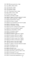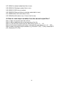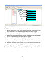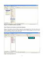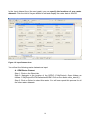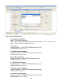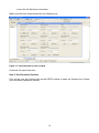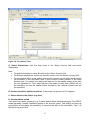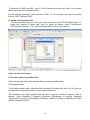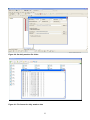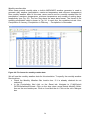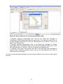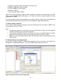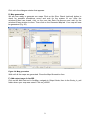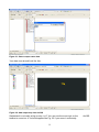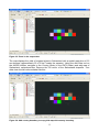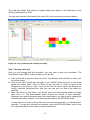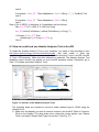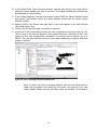
1
GIS-based Environmental Policy Integrated Climate Model GIS EPIC + User Manual Version 1.0 January 2009 GEPIC User Manual Contact Dr. Junguo Liu Swiss Federal Institute of Aquatic Science and Technology (Eawag) Ueberlandstrasse 133, CH-8600 Duebendorf, Switzerland Tel: +41-448235012 Fax: +41-448235375 Email: [email protected] [email protected] Dr. Hong Yang, Swiss Federal Institute of Aquatic Science and Technology (Eawag), Ueberlandstrasse 133, CH-8600 Duebendorf, Switzerland, Tel: 41-44-8235568, Fax: 41-44-8235375 Email: [email protected] Model objective: to simulate spatial and temporal dynamics of the major processes (e.g. crop growth, hydrological cycle, nutrient cycle, carbon cycle, erosion, climate change impact) of the soil-crop-atmosphere-management system. Citation: Users should cite the following publications for the application of the GEPIC model: Liu J., Jimmy R. Williams, Zehnder A.J.B., Yang H., 2007. GEPIC – modelling wheat yield and crop water productivity with high resolution on a global scale. Agricultural Systems 94 (2). pp 478-493. Liu J., 2009. A GIS-based tool for modelling large-scale crop-water relations. Environmental Modelling & Software 24: 411-422. * This User Manual (Version 1.0) is prepared by Dr. Junguo Liu, Mr. Franklin Uvere, and Christian Folberth. I Content 1. Overview..........................................................................................................................................1 2. Installation and preparation..............................................................................................................2 2.1 Installation..................................................................................................................................2 2.2 Preparation .................................................................................................................................2 3. Framework and file structure ...........................................................................................................3 3.1 Framework .................................................................................................................................3 3.2 File structure ..............................................................................................................................5 4. Input/Output files .............................................................................................................................8 4.1 Most important input data ..........................................................................................................8 4.2 Format of input files...................................................................................................................8 4.3 Format of output files...............................................................................................................11 4.4 How to read output variables from the annual output files? ....................................................14 5. Step by step to use GEPIC .............................................................................................................15 Example .....................................................................................................................................15 6. Advanced knowledge and functions ..............................................................................................36 6.1 How to add a crop in GEPIC ...................................................................................................36 6.2 How to add an output variable for map generation in GEPIC .................................................36 6.3 How to install and use Hawths Analysis Tool in ArcGIS........................................................37 7. Publications related to GEPIC .......................................................................................................39 1. Overview GEPIC is a GIS-based agroecosytem model integrating a bio-physical EPIC model (Environmental Policy Integrated Climate) with a Geographic Information System (GIS). The GEPIC model can be used to simulate the spatial and temporal dynamics of the major processes of the soil–crop–atmosphere-management system. The first version of the GEPIC model was developed between 2004 and 2005 to serve for a Swiss National Science Foundation funded project “Water Scarcity – Its Measurement and Implications for Virtual Water Import”. The model was developed to quantify crop yield and crop water use on a global scale with a spatial resolution of 30 arc-minutes (around 50 km by 50 km nearby the equator). Since the GEPIC model can potentially use all functions of EPIC, it has later been used to simulate impacts of climate change on crop production, green and blue water use assessments, effects of biofuel production on land and water resources, soil and water erosion etc. There are no strict classifications among different versions of the GEPIC model; hence, it is still marked as Version 1.0 so far. The GEPIC model is developed and maintained by the Swiss Federal Institute of Aquatic Science and Technology (Eawag). It is a public domain program, and as such may be used and copied free of charge for non-commercial uses. 1 2. Installation and preparation 2.1 Installation The installation process is very easy. You just need to copy the folder MyProject and all files in this folder to your hard driver C: or D:. Now you are done! Enjoy the GEPIC model. 2.2 Preparation Make sure ArcGIS 9.1 (or higher version) is installed in your computer and working properly. A basic knowledge of ArcGIS is required to use the GEPIC Model. It is possible to encounter problems when ArcGIS and ArcInfo Workstation are installed on the same machine. In this case, ArcInfo has to be removed before GEPIC can be used properly. How to start the GEPIC model: Open C:/MyProject/EPIC0509 folder (suppose you copy the folder MyProject to C: driver) and locate the file GEPIC1.0.mxd. Now you are starting the GEPIC model. Create a shortcut for this file on your desktop for later uses. The core of the simulation is the EPIC model; hence, a basic knowledge about the EPIC model is needed. The nature and format of the EPIC-required input, output and system files, as well as how to edit these files and/or create your own files, have been described in details in the EPIC User Manual. A MOnthly to DAily WEather Convertor (MODAWEC) has been developed to support GEPIC and help users to create daily weather data based on monthly weather data. When applying the MODAWEC model, please first study the MODAWEC User Manual. GEPIC only accepts raster datasets with data type of LONG (signed 32 bit) as input. When your raw raster datasets are not in this format, a Hawths Analysis Tool for GIS is frequently used to convert them to the LONG type. The Hawths Analysis Tool is a GIS extension. As to the installation and use of the Hawths Analysis Tool for GIS, please refer to 6.3. How to install and use Hawths Analysis Tool in ArcGIS 2 3. Framework and file structure 3.1 Framework Site-specific inputs Input maps and data Climate Soil Land use Irrigation DEM …. • Climate • Soil • Land use • Management Site-specific outputs EPIC GEPIC • Crop yield • ET • CWP Grid-base output maps • Yield • ET • CWP ……. ……. GIS Figure 1. General idea of the GEPIC model The general idea of the GEPIC model is expressed in Fig. 1. The EPIC model can simulate site-specific processes such as crop growth, hydrological cycle, N cycle, C cycle, climate change etc. By integrating EPIC with a GIS, the GEPIC model treats each grid cell as a site, and it simulates the above processes for all predefined grid cells with any spatial resolution. A loose coupling approach is used to integrate EPIC with a GIS. This approach relies on transfer of data files between GIS and simulation models. With this approach, the GEPIC interface abstracts most required data from GIS raster maps, edits them to the EPIC required data format. These formatted data are transferred to the EPIC model. The simulation results of the EPIC model are transferred to the GEPIC interface to generate output maps. The steps of the development of the GEPIC model are illustrated in Fig. 2. Input data are first added into GEPIC in terms of GIS raster datasets. Then, an “input data translation module” reads and writes input information to a “text input file” [input.txt]. This text input file is then used to generate specific “EPIC input files” with the help of a “UTIL” program (Universal Text Integration Language, or a data file editor that comes with the EPIC model). This process is achieved by writing command lines into a “batch file” [Temp.cmd]. By executing the batch file, GEPIC runs the EPIC model for each simulated grid cell. A set of “EPIC output files” [e.g. EPIC_OUT.OUT, EPIC_OUT.ACY etc] are generated. With an “output data translation module”, output variables are written into a series of “text output files” [e.g. 1999.txt, 2000.txt, 2001.txt etc], which are used to generate “GIS output maps”. 3 Figure 2. Schematic representation of the integration of EPIC with GIS Menu Toolbar Pop-up window Figure 3. Interface of the GEPIC model The GEPIC software comprises three components. The most obvious component is the proprietary GIS, which is a standard ArcMap window in ArcGIS 9.1. The least obvious component is the EPIC model, which is the core of all simulations. The third component is the GEPIC interface (see Fig. 3), which links GIS and EPIC. The interface contains toolbars and menus. The toolbars provide functional buttons to (1) locate raster input data 4 sets; (2) select the simulated area and crops; (3) specify spatial resolution; and (4) set the locations of the EPIC file, and input and output files. It further provides buttons to (1) edit inputs into EPIC required input files; (2) run the EPIC model; and (3) to generate output maps. The menu has submenus, which allow users to perform the same tasks as the toolbar. The ESRI’s GIS software ArcGIS9.1 was selected to develop the GEPIC model. ArcGIS is used as an application framework, input editor, and map displayer. As an application framework, ArcGIS provides the main programming language VBA to design the interface of GEPIC, and to design programs for input data access, text output data generation, and output map creation. As an input editor, ArcGIS is used to convert vector input data into raster data, which are the main input format. One typical example is the climate data. Daily climate data are often available for various stations, while the code of each station is presented as attributed point data. The point data is converted into raster data with a method of Thiessen Polygons, with which the daily climate data from the closest climate station is used as a representative for a grid cell. As a map displayer, ArcGIS can be used to visualize the GIS data (e.g. vector or raster input data; raster output data etc). 3.2 File structure As a first step to start the model, users need to know (1) the location of the GEPIC software; (2) the file structure; (3) the location of the executable file. A. Location of the GEPIC software Figure 4. Location of GEPIC software 5 B. File structure The file structure is shown in Fig. 5. Data EPIC0509 Input Output \Data: all the input datasets \EPIC0509: executive file, all EPIC related files, annual output file for specific year \Input: back up of input information \Output: location for output maps Figure 5. The file structure of GEPIC Major files in the folder EPIC0509 include GEPIC Executive file: GEPIC1.0.mxd EPIC related files - EPIC executive file: EPIC0509.exe - EPIC code: EPIC0509.for - Most detailed EPIC output file: *.out - All other EPIC input and output files Text input file [input.tx] Annual output for specific year: e.g. 2000.txt File structure is demonstrated in the schematic representation of the integration of EPIC with GIS, shown in the following chart. 6 Data DEM GIS Input Datasets Soil databases Slope Soil Meteorological databases Climate Land use Irrigation GIS Output Maps Others Output Yield Y ET ArcGIS 9 CWP N Input Data Translation Module End of Grid Simulation Text Output files (ET/Y/CWP) Output Data Translation Module Text Input Files Input UTIL EPIC Input Files EPIC EPIC Output Files Batch File EPIC0509 Figure 6. File structure in the schematic representation of the integration of EPIC with GIS. C. Location of GEPIC executable file (see Fig. 7) Figure 7. Location of GEPIC executable file 7 4. Input/Output files 4.1 Most important input data Soil parameters: each soil type (or soil code) should have one separate soil file (*.sol). The soil file has a strict format which has been explained in EPIC User Guider v. 0509 on page 18-19. Soil parameters should be prepared as many as possible, and the following ones have to be included: depth, percent sand, percent silt, bulk density, pH, and organic carbon content. Users need to give a number for each soil file name (e.g. 3201.sol). The number is indicated in the soil code map (or Soil Raster Dataset). Climate parameters: daily weather data file (*.dly) and monthly weather statistics file (*.wp1) are needed. Users should give a same number for two corresponding weather files (e.g. 66100.dly and 66100.WP1). The number is indicated in the climate code map (or Climate Raster Dataset). Daily weather data file (*.dly) The format of the daily weather data file is described on page 21 in EPIC User Guider v. 0509. Daily weather parameters include solar radiation, max temperature, min temperature, precipitation, relative humidity and wind velocity. Monthly weather statistics file Once you have the daily data, a WXPM3020 program can be used to generate the monthly weather statistics. Details please refer to page 21-23 in EPIC User Guider v. 0509. Irrigation data and fertilizer data (N is most important) are very important for crop yield and crop water use. Users should provide data on total annual amount of irrigation (in mm/yr) and annual fertilizer application (in kg/ha). 4.2 Format of input files Three types of input data are needed for the GEPIC model: GIS raster datasets, text files and user-specified data. The most important input data are GIS raster maps. They should be set in the Input Datasets form (Fig. 8). Necessary maps include: DEM raster dataset: the average elevation in each grid cell Slope raster dataset: the average slope (in %) in each grid cell (e.g. 8 means the slope is 8% in a grid cell) Country raster dataset: code number of different region. The default map shows the code number of each country. Land use raster dataset: this map provides information on crop distribution. In the land use map, only three numbers should be included: 0 indicates absence of a specific crop, while 1 and 2 indicate existence of the crop under rainfed and irrigated conditions, respectively; Soil raster dataset: code numbers of the soil files in each grid cell Climate raster dataset: code numbers of the climate files in each grid cell Irrigation raster dataset: annual maximum irrigation depth in mm/yr. When data are not available, select “No Data” button under the irrigation map input panel. Fertilizer raster dataset: annual maximum fertilizer application rate in kg/ha. 8 Figure 8. Pop-up window for setting input raster datasets The second type of input data is text files. Weather and soil data are stored in text files. Weather data: when daily weather data are available, each climate code corresponds to two weather text files: (1) daily weather text file containing daily weather data (e.g. daily precipitation, daily minimum and maximum temperatures), and (2) monthly statistics text file which contains information on monthly weather statistics. When monthly weather data are available, each climate code corresponds to at least four text files, which contain monthly data on (1) precipitation; (2) maximum temperature; (3) minimum temperature; and (4) number of wetting days. Soil data: each soil code corresponds to one soil text file, which contains several soil parameters (e.g. soil depth, percent sand and silt, pH, organic carbon content, etc) (see Fig. 9). The format of the soil file is shown in page 18-19 in the EPIC User Manual. Users need to prepare the weather and soil data files. For large-scale studies, users should prepare a large number of data files. In this case, they may need to write a computer program to help them create these files. 9 Figure 9. Soil data files and their format. The third type of input data is the user-specified data in pop-up windows in the GEPIC interface (e.g. in Fig. 10). Users just need to complete the forms. When users close the windows, the input information in the forms is saved automatically by the GEPIC model. Figure 10. Options form 10 4.3 Format of output files The main outputs of the GEPIC model are raster GIS maps representing the spatial distribution of output variables such as crop yield and evapotranspiration. The rules for the output maps are as follows: Variable code and meaning yd: yield et: seasonal ET wp: crop water productivity bm: biomass t: transpiration i: irrigation hi: harvest index n: N fertilizer input aet: annual ET Name format of the output maps: one specific year: variable code _ year [e.g. yd_1995] average of multiple years: variable code_startyear_endyear [e.g. yd_1995_2000] The variable codes are used to give names to maps (see name format of the output maps). The GEPIC always use the names with the above format. The output maps are saved in the folder specified by users in the Map Generation Form (see Fig. 28: Step 3 Select folder to save maps). In case you want to change the output map names, use ArcCatelog to do so. Another kind of GEPIC outputs are “text output files” [e.g. 2000.txt, 2001.txt. The names depend on the simulation period set by users]. These files are used to generate the above output maps. In each text file, one line shows the results of 62 variables for one grid cell. Variables are separated with a comma in the output files (see the following graph for output format). 11 V1 V2 V3 …… Figure 11. Format of text output file The output variables include: V1: Longitude V2: Latitude V3: Crop yield (t/ha) V4: Ratio of crop yield to growing season ET (kg/mm) V5: ETGS (Growing season ET in mm) V6: GSEF (Growing season plant transpiration in mm) V7: SMY(19) (Irrigation volume in mm) V8: FGIS (N fertilizer applied in kg/ha) V9: SMY(11) (Actual ET in mm) V10: GSVF (Growing season vapour pressure deficit in KPa) V11: HGIS (Crop harvest index) V12: SRAF (Growing season solar radiation in MJ/m2) V13: YLNG (N content of crop yield in kg/ha) V14: TNGS (N content of soil in kg/ha) V15: X2 (N lost to atmosphere in kg/ha) V16: X3 (N lost with runoff, subsurface flow, and erosion in kg/ha) V17: SMY(42) (Wind erosion in t/ha) V18: SMY(NDVSS) (water erosion for driving EQ in t/ha) V19: SMY(3) (Solar radiation in MJ/m2) 12 V20: BGIS (Biomass production in t/ha) V21: SF1 (Water stress in days) V22: SF2 (N stress in days) V23: SF3 (P stress in days) V24: SF4 (K stress in days) V25: SF5 (Temperature stress in days) V26: SF6 (Aeration stress in days) V27: SF7 (Salt stress in days) V28: SMY(46) (N leached in kg/ha) V29: SMY(43) (Organic N loss with sediment in kg/ha) V30: SMY(47) (Net mineralization in kg/ha) V31: SMY(49) (Denitrification in kg/ha) V32: SMY(50) (N fixation in kg/ha) V33: SMY(85) (N mineralization from humus in kg/ha) V34: SMY(51) (Nitrificaiton in kg/ha) V35: SMY(52) (Volatilization in kg/ha) V36: SMY(53) (N loss in drainage system in kg/ha) V37: SMY(54) (P loss with sediment in kg/ha) V38: SMY(56) (P mineralization in kg/ha) V39: SMY(57) (P leached in kg/ha) V40: SMY(58) (Enrichment ratio) V41: SMY(59) (N fertilizer organic form in kg/ha) V42: SMY(60) (N fertilizer NO3 form in kg/ha) V43: SMY(61) (N fertilizer NH3 form in kg/ha) V44: SMY(62) (P fertilizer organic form in kg/ha) V45: SMY(63) (P fertilizer mineral form in kg/ha) V46: YLPG (P content of crop yield in kg/ha) V47: YLKG (K content of crop yield in kg/ha) V48: SMY(77) (Organic C loss with sediment in kg/ha) V49: SMY(4) (Precipitation in mm) V50: SMY(17) (Percolation in mm) V51: SMY(14) (Runoff in mm) V52: SMY(5) (Snowfall water equivalent in mm) V53: SMY(6) (Snowmelt in water equivalent in mm) V54: SMY(10) (Potential ET in mm) V55: SMY(12) (Potential plant transpiration in mm) V56: SMY(13) (Actual plant transpiration in mm) 13 V57: SMY(16) (Lateral subsurface flow in mm) V58: SMY(18) (Drainage system flow in mm) V59: SMY(15) (SCS curve number) V60: SMY(20) (External inflow to maintain water table in mm) V61: SWGS (Root zone soil water in mm) V62: SMY(68) (Soil water in top 10 mm of soil in mm) 4.4 How to read output variables from the annual output files? Step 1: Open an annual output file in Excel Step 2: Add an additional row at the beginning of the file Step 3: In the first line of the Excel file, add column code 1, 2, … 62 Step 4: Find output variables with these codes and the code above (V1, V2… V62) Step 5: Read your target output variables, e.g. Annual ET (V9), T (V56), Seasonal ET (V5), Reference ET (V54) 14 5. Step by step to use GEPIC Example Assuming you would like to simulate crop yield of irrigated wheat in Switzerland on a 0.5o resolution in 2000 and 2001. You need to prepare the following raster datasets: Land use map (crop distribution map) for wheat in Switzerland Soil code map Climate code data Slope map Digital Elevation Model (DEM) map Country code map Annual irrigation depth for wheat Fertiliser application rate for wheat Make sure that: All the above datasets have the same spatial resolution as that specified for your simulation. Users need to specify the simulation resolution in the Options window for GEPIC; All the above datasets should have the data type of LONG. When your raw data are not with this data type, you need to convert to this type by using Hawths Analysis Tools; When you do not have irrigation data, select the No Data Check Box. The model will assume sufficient irrigation for the grid cells under irrigated systems. The above datasets have been prepared in the ‘DATA’ folder for demonstration. Please follow the steps for using the GEPIC model. Step 1: Open the GEPIC file Open the GEPIC1.0.mxd file from the shortcut you created on your desktop, or from C:\MyProject\EPIC0509\GEPIC1.0.mxd. An ArcGIS window opens. You can locate GEPIC Toolbar in the window. 15 Save Runs Map Generation Simulation Write All Input Data Options Set Input Data Figure 12. The GEPIC toolbar The GEPIC toolbar contains six major functional buttons (Fig. 12): 1) Set Input Data: clicking on this button opens the Input Data Form, where you can specify the location of your raster datasets and display your data in ArcGIS. 2) Options: clicking this button opens the Setting Simulations Options Form, where you can select your simulation options. 3) Write All Input Data: clicking this button will send commands to read raster datasets and write all input information into the text input file “input.txt”. 4) Simulation: clicking this button will open the Auto Calendar window, where you can select fixed crop calendar or automatic crop calendar for your simulation. 5) Map Generation: clicking this button will open the Map Generation form, where you can generate maps from output data. 6) Save Runs: clicking this button will open a form to help save your simulation runs. If the GEPIC toolbar is not within the ArcGIS system, click on the View menu on your ArcGIS menu. Scroll down to Toolbars in the drop down menu and make sure GEPIC Toolbar is ticked. If it is not, click on it to display the GEPIC toolbar (please follow Fig. 13). You can then customise the location of the toolbar. 16 Figure 13. Set GEPIC toolbar in ArcGIS Step 2: Specify the location of your raster datasets Click on the toolbar Set Input Data to open the Input dataset form. The first tab on the GEPIC toolbar is called the Set Input Data (see the following graph). Put your cursor above the first tab and you will see the name. Set Input Data Figure 14. Set Input Data Tool 17 In the Input dataset form (the next graph) you can specify the locations of your raster datasets. Click the Add to Layers button to add and display the raster data in ArcGIS. Figure 15. Input Dataset form You will set the following raster datasets as input: A. DEM Raster Dataset Step 1: Click on the Reset tab. Step 2: Navigate to the location of the GEPIC (C:\MyProject). Open folders as follows: C:\MyProject\DATA\Switzerland\DEM. Click on the raster swiss_dem30_l. Step 3: Click on Select to select this raster. You will now repeat this process for all the other raster datasets. 18 Figure 16 Select DEM dataset B. Slope Raster Dataset Step 1: Click on the Reset tab. Step 2: Navigate to C:\MyProject\DATA\Switzerland\Slope. Click on swiss_slpe_l. Step 3: Click on Select to select this raster. C. Country Dataset Location: C:\GEPIC\DATA\Switzerland \Country Dataset Name: swiss_count_l D. Landuse Raster Dataset Dataset Location: C:\GEPIC\DATA\Switzerland \Landuse Dataset Name: swiss_irwt_l E. Soil Raster Dataset Dataset Location: C:\GEPIC\DATA\Switzerland \Soil Dataset Name: swiss_soil_l F. Climate Raster Dataset Dataset Location: C:\GEPIC\DATA\Switzerland \Climate Dataset Name: swiss_clim_l G. Fertiliser Raster Dataset Dataset Location: C:\GEPIC\DATA\Switzerland \fertiliser Dataset Name: whtferti_1 H. Annual Irrigation Depth Dataset Location: C:\GEPIC\DATA\Switzerland \Irrigation Dataset Name: max_irr_2000. 19 Leave the No Data box unchecked. Make sure the form looks exactly like the following one. Figure 17. Input datasets for this example Close the Set Input Data form. Step 3: Set Simulation Options Click on the next tab (Options tab) on the GEPIC toolbar to open the Options form. Select your simulation options as follows: 20 Figure 18. The options Form A. Select Switzerland: click the drop arrow in the Select Country field and select Switzerland. Note: For global simulations, select World from the Select Country field. For national simulations, select one specific country from the Select Country field. For simulations which cover neither one specific country nor the entire world, define the boundary of the simulation area in the Landuse Raster Dataset in the Input dataset form. You should only define the land use for the spatial extent of the area you are interested in. Then, select World in the Select Country field. GEPIC will run the simulation for only the spatial extent covered by the Landuse Raster Data set you specified. B. Set the simulation spatial resolution. In this case our grid size is 0.5 degrees. C. Select wheat in the Select crop field D. Set simulation period You need to set warm-up period (e.g. 3 years) before actual simulations begin. The GEPIC model generally creates unreliable results in the first few years. This setting of warm-up period aims at minimising the possibility of errors at the start of the simulation. Type 3 in the Warm-up years field 21 To simulate for 2000 and 2001, type 2 in the Simulations years field. Note: Your climate data must cover the simulation period. So the starting simulation year should be 1997. In this example, the warm-up period include 1997, 1998 and 1999. E. Set up soil parameter files The soil parameter files for all the grid cells are saved in the EPICSoilWise folder. To select the location of these files, click on Reset as before. Open C:\MyProject\ DATA\Switzerland\Soil. Then click on EpicSoilWise and on ok to select it. Figure 19. Set soil file folder F. Set the location of weather files Users can provide either daily weather data or monthly weather data. Daily weather data To set daily weather data, check the Daily weather file location box (see Fig. 20) and use the reset tab to select the location of your daily weather file. The variables in the daily weather files are Year (6 spaces), Month (4 spaces), Day (4 spaces), Solar Radiation (6 spaces), Maximum Temperature (6 spaces), Minimum Temperature (6 spaces), Precipitation (6 spaces), Relative Humidity (6 spaces), and Wind Speed (6 spaces) (Fig. 21). 22 Figure 20. Set daily weather file folder Figure 21. File format for daily weather data 23 Monthly weather data When users provide monthly data, a built-in MODAWEC weather generator is used to generate daily weather (precipitation, maximum temperature and minimum temperature) from monthly weather data. In this case, users need to set four monthly weather files for precipitation, maximum temperature, minimum temperature and number of wetting days, respectively (see Fig. 26). The four files share the same data format. The format of the monthly precipitation data is shown in Fig. 24. In each line, the variables include Year, Precipitation in January, Precipitation in February … Precipitation in December. Figure 22. File format for monthly weather data We will use the monthly weather data for this simulation. To specify the monthly weather files locations: Check the Monthly Weather files location box. If it is already checked do not uncheck it. In the Precipitation field click on the Reset tab. Navigate to C:\MyProject\ DATA\Switzerland\Climate. Click on the drop down arrow beside Monthly folder, then on the one beside prec. Click on Land and the ok. Click on the ok in dialogue box. 24 Figure 23. Select folder to set monthly precipitation data Monthly maximum temperature files: click on the Reset tab. Navigate to C:\MyProject\ DATA\Switzerland\Climate again and in the Monthly folder click on the arrow beside the folder tmx. Click on Land and then ok to select it. Click on ok again in the dialogue box. Monthly minimum temperature: click on the Reset tab. Navigate to Climate folder again and in the Monthly folder click on the arrow beside the folder tmn. Click on Land and then ok to select it. Click on ok again in the dialogue box Number of wet days: click on the reset tab in the Wet days field. Navigate to Climate folder. Under the Monthly folder, click on the arrow beside wet. Click on Land, then ok and ok again. You are now through with selecting your main options. Make sure your form looks exactly like this: 25 Figure 24. Complete the Options form Close the Options form. Step 4: Writing your input data At this stage, you need to write all your input data. The third toolbar called the Write All Input Data (placing your cursor on this button will reveal its name) is needed for this purpose. Click on the Write All Input Data tool to write and save all your input data. Now the input data are saved to the text input file input.txt. 26 Figure 25 Save input data Note: To be sure that your input files have all been written, open the EPIC0509 folder. Scroll to the input.txt file, open it (this can be done using Notepad) and make this file empty. Then click the button Write All Input Data. You should have some input in input.txt. An empty file means you fail to write input in this file. In case that you have an empty input.txt, please check: Land use raster dataset: it should contain only three numbers: 0, 1 and 2; C:\MyProject folder. You should have this folder. Some users change the folder name to GEPIC. This will lead to failure of simulation. Please keep the folder “C:\MyProject”; Check the type of input raster datasets. Make sure the type is LONG No data: for example, in the demonstration verion, we only provide data for Switzerland. When you select a country rather than Switzerland (e.g. China), GEPIC will not write anything to input.txt. You need to prepare data first! Step 5: Run your simulation. The fourth toolbar is the Simulation tool. Click on the Simulate tab, and an Auto Calendar window shows up. If you run a simulation for which exact planting and harvest dates are known, you can select the Fixed Crop Calendar option. In this case, you will need to specify the planting and harvesting dates in the crop operations *.ops (see EPIC user manual) file in the EPIC0509 folder. When exact planting and harvest dates are not available, check the Automatic Crop Calendar box Make sure your view looks exactly like this: 27 Figure 26. Auto calendar form Click on the Simulate tab. The following windows32.exe window will show up. Figure 27. A window for model simulation Note: you must leave the windows32.exe window open. Closing it will terminate the simulation. At the end of the simulation this window closes by itself. 28 This simulation will take about 10 minutes. It could last longer or shorter, depending on the speed of your computer. Certainly, when you simulate for a larger area (e.g. the entire world) with higher spatial resolution, it will take much longer time. Step 6: Generate your output maps When the windows32.exe window has closed at the end of the simulation, it is now time to generate the yield map. The fifth button is the Map Generation tool. You will generate your yield map with it. You can also create other maps, depending on the output variables you are interested in. Figure 28. Map generation form A. Open Map Generation form Click on the Map Generation button, the Map Generation form opens (Fig. 30). B. Select variables You can select any variables for map generation by clicking on each variable in the All Variables column and using the directional arrow to send it into the Variables for Map Generation column. You can also deselect any of the variables in the Variables for Map Generation column by clicking on it and using the directional arrow to send it to the All Variables list. The following variables are included in the All Variables list: Yield: crop dry yield in kg/ha CWP: crop water productivity (CWP=yield/ET in kg/m3). HI: Harvest Index Biomass: biomass generation in kg/ha. Annual ET: annual evapotranspiration in mm 29 Irrigation: irrigation water requirement of crop in mm Nitrogen application rates in kg/ha N_soil: nitrogen in soil in kg/ha Biomass in kg/ha Yield: crop dry yield in kg/ha. When you need to generate maps for other variables, add them in the above form yourselt. This is easy. Please follow the steps in 6.2 How to add an output variable for map generation in GEPIC. For this exercise we are only interested in crop yield. Click on Yield in the All Variables list and use the directional arrow to send it to the Variables for Map Generation list. C. Select period of interest In the Step 2 (Select Period) segment, check the Multi-years box and type in 2000 in the From and 2001 in the To field. Note: To generate maps for one specific year you would need to check the One Specific Year box and then type in the year of interest. To generate individual maps for more than one year, you should check the Multiyears box and then type in the years of interest in the From and To fields. Make sure the years selected are within the simulation years range selected in the Options form. D. Select folder to save output maps In the Step 3 Select Folder To Save Map segment, click on the Set a new folder tab. Navigate to “C:\MyProject\Output”. Click on the My Output folder and click ok. Figure 29. Select folder to save output maps 30 Click ok in the dialogue window that appears. D. Map generation We are now ready to generate our maps. Click on the Error Check (optional) button to check for possible simulations errors and wait for the system to run. After the windows32.exe has closed, click on the next tab Data Pre-process and wait for the windows32.exe window to close. Then click on the Generate Map tab. Your map will now be generated (Fig. 30). Figure 30. Map generation Wait until all the maps are generated. Close the Map Generation form. F. Add output maps in ArcGIS Click on the Add Data tool in ArcMap, navigate to Output folder, then to the Swiss_irr_wht folder where your map was saved. Click on yd2000. 31 Figure 31. Select output raster data Your data view should look like this: Figure 32. Add output map into ArcGIS Switzerland is not really a big country, is it? You can use the zoom tool on the toolbar to zoom into it. It should appear like Fig. 33 if you zoom it sufficiently: 32 ArcGIS Figure 33. Zoom in the output data The map displays the yield of irrigated wheat in Switzerland with a spatial resolution of 0.5 arc degrees (approximately 50 x 50 km2 nearby the equator). Using the Add Data tool on the ArcGIS toolbar, navigate to the Country folder (in the DATA folder) and add map of Switzerland, switzerland.shp. Remove the Fill colour of the Switzerland shapefile. Your data view should look somewhat like this: Figure 34. Add country boundary to crop yield map with country boundary 33 The yield map shows that yields of irrigated wheat were higher in the North than in the South in Switzerland in 2000, You can also view the Yield map for the year 2001 in the same way mentioned above. Figure 35. Crop yield map with country boundary Step 7: Saving your runs Once you are through with this simulation, you may wish to save your simulation. The Sixth button in the GEPIC toolbar enables you to do this. A. Click on this tab to open the Save Run form. You will then select a folder in which your run will be saved. B. Click on the Set A Folder tab. Navigate to your GEPIC folder and click on the arrow beside the Output folder. Click on Swiss_irr_wht and click ok. Click ok again in the dialogue box and click on Save. Your run will now be saved. When the window.exe closes, close the SaveRunsForm. Now you can view your run files in the folder you selected. C. Open the Swiss_irr_wht folder. You should have one Autocalendar folder and eight other files in it. The Autocalendar folder contains the results of your simulation. Whenever you wish to generate maps form these results, you can do so by copying the Autocalendar folder contents to the Autocalendar folder in the EPIC0509 folder. In case that one or more of these files are not saved automatically, you should save it manually. To copy any of these files manually, open the EPIC0509 folder, scroll to the file, copy and paste it to the folder you plan to save files. 34 Figure 36. Save your runs 35 6. Advanced knowledge and functions 6.1 How to add a crop in GEPIC The following texts show the steps to add crop tomato in the GEPIC model. When you plan to add a different crop, you need to follow the same steps but should change the places with pink colour. Step 1: Edit TOMA.opc file and add to the folder “\EPIC0509” Step 2: Add the file name to \EPIC0509\OPSCCOM.DAT (“44 TOMA.OPC”) Step 3: Add the crop name in \EPIC0509\CROP.TXT (“tomato”) Step 4: In GEPIC -> AutoCalendarForm -> Simulate, add the following (Location: above the sentence “' ADD THE CROPS YOU PLAN TO SIMULATE” If InputTextFileForm.ComboBox2 = "tomato" Then iCropCode = 44 ‘crop code in crop.txt file Open sCropCMD For Append As #1 Print #1, "util run epicrun.dat iops(1)=" & 44 ‘crop code in crop.txt file Close #1 sOPSC = "toma.opc" End If ----- Above “ADD THE CROPS YOU PLAN TO SIMULATE If InputTextFileForm.ComboBox2 = "tomato" Then If iCropCode <> 44 Then 'crop code in crop.txt file iCropCode = 44 Print #FilNum, "util run epicrun.dat iops(1)=" & 44 'crop code in crop.txt file End If End If -------Note: it’s necessary to copy TOMA.opc, OPSCCOM.DAT, and CROP.TXT to the EPIC0509 folder where you plan to run the program. -------- 6.2 How to add an output variable for map generation in GEPIC The following texts show the steps to add the variable ET for map generation. When you plan to add a different variable, you need to follow the same steps but should change the places with pink colour. In the following example, Ann_ET is the text shown in the Map Generation Form (Fig. 28, All variables text box). aet is the variable code (see 4.3 Format of output files) Step 1: The output variable has to be included in the annual output files (e.g. 1995.txt, 1996.txt etc). If not, users have to edit EPIC0509.FOR file to generate this variable in the annual output files. Step 2: Go to GEPIC Modules OpenMapGenFormMod, add .AddItem "Ann_ET" Step 3: Go to GEPIC Forms MapGenForm, Click button “Generate Maps”, add the follows If sVariable = "Ann_ET" Then sMapName = "aet" + CStr(j) + "_" + TextBox3.Text ‘Add 1 If sVariable = "Ann_ET " Then sMapName = "aet" + CStr(j) 36 ‘Add 2 If sVariable = "Ann_ET " Then sMapName = "aet" + CStr(j) + "_" + TextBox3.Text ‘add 3 If sVariable = "Ann_ET " Then sMapName = "aet" + CStr(j) ‘add 4 Step 4: Go to GEPIC Modules CreateMaps, add the follows Dim Ann_ET(0 To 1000, 0 To 1000) As Long Ann_ET(intCol(TotCellNum), intRow(TotCellNum)) = CLng(ET) If Content = "Ann_ET" Then vSafeArray(i, j) = CLng(Ann_ET(i, j)) End If 6.3 How to install and use Hawths Analysis Tool in ArcGIS To install the Hawths Analysis Tool in your computer, you need to first download it from http://www.spatialecology.com/htools/download.php, and then install it. After the installation, you should find an extension called Hawths Analysis Tools in ArcGIS (ArcGIS Tools Extensions). Make sure this extension is selected. The Hawths Analysis Tool dropdown menu should now appear on your ArcGIS standard toolbar. Otherwise, go to View Toolbars and select Hawth’s Tools. Figure 37. Interface of the Hawths Analysis Tools The following steps are needed to convert a raster dataset type to LONG using the HawthsTools: A. Make sure the dataset you wish to convert is listed in the ArcGIS Table of Contents. Click on the Hawths Tool drop down menu, place the mouse pointer over “Raster Tools” and select “Raster Data Type Conversion” (See Fig. 37). 37 B. In the Raster Pixel Type Converter window, use the drop arrow in the Input field to select the raster dataset you wish to convert. The original dataset type should now be displayed in a frame below. C. In the Output segment, use the drop arrow to select GRID as Output dataset format and specify the location where the raster dataset should now be saved (raster dataset location). D. Select LONG in the Output data type field; a value will appear in the New NoData Value field, ignore this. E. Click on OK for the data type conversion to proceed. F. At the end of the conversion process, an error message may pop-up (see Fig. 38). This is a bug in the Hawths Analysis Tools. Ignore this error, and click on OK. Your raster, by now, has already been converted. You should now be able to use it in GEPIC. You can also add and view your new raster dataset by using the Add Data toolbar in ArcGIS. Figure 38. Error message from the Hawths tool Note: In case of an error messages different from the one shown above, restart the procedure and check the file name you gave for your new raster dataset. Make sure the file name does not exceed 13 characters. 38 7. Publications related to GEPIC Peer-reviewed Journal Publications 1. Liu J., Jimmy R. Williams, Zehnder A.J.B., Yang H., 2007. GEPIC – modelling wheat yield and crop water productivity with high resolution on a global scale. Agricultural Systems 94 (2). pp 478-493. 2. Liu J., Wiberg D., Zehnder A.J.B., Yang H., 2007. Modelling the role of irrigation in winter wheat yield and crop water productivity in China. Irrigation Science 26 (1). pp 21-33. 3. Liu J., Zehnder A.J.B., Yang H., 2008. Drops for crops: modelling crop water productivity on a global scale. Global NEST Journal 10 (3): 295-300. 4. Liu J., Williams J.R., Wang X., Yang H., 2009. Using MODAWEC to generate daily weather data for the EPIC model. Environmental Modelling & Software 24(5): 655664. 5. Liu J., 2009. A GIS-based tool for modelling large-scale crop-water relations. Environmental Modelling & Software 24: 411-422. 6. Liu J., Fritz S., van Wesenbeeck C.F.A., Fuchs M., Obersteiner M., Yang H., 2008. A spatial explicit assessment of current and future hotspots of hunger in SubSaharan Africa in the context of global change. Global and Planetary Change.64 (34): 222-235. Other Publications 7. Liu J., Yang H., 2008. The impacts of global climate change on irrigation water requirement of wheat in China. In: Proceedings of the 13th IWRA World Water Congress. Montpellier, France, 1-4 September 2008. 8. Liu J., 2007. Modelling global water and food relations – development and application of a GIS-based EPIC model. PhD Thesis. DISS. ETH NO.17069. Swiss Federal Institute of Technology Zurich, Zurich, Switzerland. 9. Liu J., Yang, H., Zehnder A.J.B, 2007. Simulation of crop water relations on large scales with high spatial resolutions. In: van Bers C., Petry D., Pahl-Wostl C. (Eds.), Global Assessments: Bridging Scales and Linking to Policy. GWSP issues in global water systems research No. 2: 44-48. The Global Waster System Project. Bonn, Germany. 10. Liu J., Zehnder A.J.B., Yang H., 2007. Drops for crops: modelling crop water productivity on a global scale. pp A835-842. In: Lekkas T.D. (ed) Proceedings of the 10th International Conference on Environmental Science and Technology. Kos Island, Greece, 5-7 September 2007. ISSN: 978-960-7475-40-4. 11. Liu J., Zehnder A.J.B., Yang H., 2006. Global crop water productivity simulation for wheat – an application of the GEPIC model. pp 13-14. In: World Congress: Agricultural Engineering for a Better World: The proceedings of the 2006 World Congress. Congress, Bonn, Germany, 03-07 September 2006. ISBN: 3-18-0919582. 12. Yang H., Liu J. Zehnder A., 2005. Optimiertes Wassermanagement in der weltweiten Nahrungsmittelproduktion. Eawag Jahresbericht 2005: 30. Papers under Review 13. Liu J., Zehnder A.J.B., Yang H., 2009. Global consumptive water use for crop production: the importance of green water and virtual water. Submitted to Water Resources Research. 14. Liu J., Yang H., 2009. Spatially explicit assessment of global green and blue water uses in cropland. Submitted to Journal of Hydrology. 39