Download A new theory of Aharonov-Bohm effect with a variant

Annales de la Fondation Louis de Broglie, Volume 27, no 3, 2002
529
A new theory of the Aharonov-Bohm effect
with a variant in which the source of the
potential is outside the electronic
trajectories.
GEORGES LOCHAK
Fondation Louis de Broglie, 23, rue Marsoulan, F-75012 Paris
ABSTRACT. A new theory of the Aharonov-Bohm experiment, based o n
the calculation of the phase difference between the electronic trajectories,
shows that the shifting of the interference fringes depends both on the
gauge of the potential and of the location of its source with respect to the
interference device. A new experiment is then suggested, in which the
source of the potential is outside the electronic trajectories. The line
integral of the potential along the trajectories equals zero, but the shifting
ofthe fringes does not vanish.
RÉSUMÉ. Une nouvelle théorie de l’effet Aharonov-Bohm, basée sur le
calcul de la différence de phase entre les trajectoires électroniques montre
que l’effet dépend à la fois de la jauge du potentiel et de la position de la
source par rapport au dispositif interférentiel. On propose ensuite une
nouvelle expérience dans laquelle la source du potentiel est extérieure
aux trajectoires. L’intégrale du potentiel le long des trajectoires est nulle,
mais le déplacement des franges subsiste.
1
INTRODUCTION
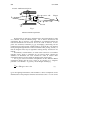
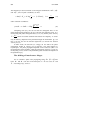
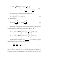
The Aharonov-Bohm experiment [1], [2], [3] was conceived in order to
prove the effect of a fieldless magnetic potential on electronic interferences.
The idea was to introduce, between the electronic trajectories coming from
two virtual coherent sources, a magnetic string, or a thin solenoid,
orthogonal to the trajectories and long enough, so that the magnetic field
emanating from the extremities cannot modify the electron trajectories (Fig.
1).
530
G. Lochak
Fresnel - Möllenstedt biprism
1
S
2
++ +
+ +
++
h k = p = mv - eA
fringes
solenoid
F
h k = p = mv + eA
screen
Fig. 1
Aharonov-Bohm experiment
Theoretically, in order for a magnetic flux to be trapped inside a string
or a solenoid, it must be infinitely long : this is what is assumed in the
calculations. But in practice, a few millimeters are sufficient because the
transverse dimensions of the device are on the order of microns. As this
point was contested, Tonomura [2], [3] succeeded in substituting for the
rectilinear string a microscopic toroidal magnet ( ∅ ≈ 10 µm ), one electron
beam passing through the hole of the torus and the other passing outside, so
that the magnetic lines may be regarded as beeing entirely enclosed in the
magnet.
Nevertheless, in what follows, we shall restrict ourselves to an infinite
magnetic string, which is sufficient for our present object, because the
subtleties of Tonomura tori were invented in order to answer other
arguments than those we are aiming at refuting in the present paper.
Let us give at first an intuitive interpretation of the Aharonov-Bohm
experiment. Recall that the wave vector of an electron in a magnetic
potential - even fieldless - is given by the de Broglie formula [5]:
h
n = hk = p = mv + eA
λ
(1)
( p is the Lagrange momentum). This formula is a direct consequence of the
identification of the principles of Fermat and of least action : it is one of the
A new theory of the Aharonov-Bohm effect with a variant …
531
most reliable results of quantum mechanics. Therefore, it is a priori obvious
that interference and diffraction phenomena will be influenced by the
presence of a magnetic potential, independently of the presence or not of a
magnetic field.
This phenomenon follows from a simple change of wavelength and
thus a change of phase, as may be done in optics by introducing a plate of
glass into a Michelson interferometer. Besides, the phenomenon is
manifestly gauge dependent : if we add something to A , whether it be a
gradient or not, λ is modified. Of course, it is true even when A = 0 , i.e.
for the formula
λ=
h
in the vacuum, which is thus gauge dependent
mv
too. This fact was emphasized by de Broglie many years ago : electron
interferences are not gauge invariant.
In the case of the Aharonov-Bohm experiment, there are additive
phases on both interfering waves, and moreover they are in opposite
directions, which doubles the shift of interference fringes. We furthermore
give a new proof of all this.
This remarkable effect, which proves the influence of a fieldless
magnetic potential on electron waves, is shocking for those who have been
convinced for a century that electromagnetic potentials are only mathematical
intermediate entities. And even more shocking is the fact that formula (1)
imposes an electromagnetic gauge that can be measured experimentally.
The almost unanimous opinion that gauge invariance is an absolute
law is so firmly fixed in prevailing thought that even distinguished
physicists [4] are led to present a wrong formula for the wavelength –
writing
λ=
h
instead of formula (1), in the presence of a potential. For
mv
the same reason, Feynman managed to relate the Aharonov-Bohm effect, not
with the wavelength formula (1), but with the magnetic flux trapped in the
string or in the solenoid, saving in this way the gauge invariance [6], [7].
The aim of the present work is to prove that the shifting of the fringes
depends on the distance from the solenoid to the experimental device and to
suggest a new experiment in which the solenoid, with its magnetic flux, is
outside the quadrilateral formed by the electronic trajectories, which causes
the integral of A to vanish and makes the argument of the magnetic flux
enclosed by the trajectories ineffective.
Actually, the quadrilateral itself will be removed from the calculations,
rejecting to infinity the electron source and the interference fringes, which
introduces negligible errors : this approximation is usual in optics.
532
2
G. Lochak
A NEW THEORY OF THE AHARONOV-BOHM
EFFECT
The commonly admitted theories of this effect are often complicated
[2] but for the physical bases, one can read the brillant book of Tonomura
[3]. Actually, the geometrical optics approximation is sufficient to answer
the true question : "Where are the fringes ?". This is why we shall make use
of it, assuming that we are in the case of Young slits : the other cases are
topologically equivalent.
We shall define the phase of the de Broglie wave as :
ϕ=
S
h
(2)
where S is the principal Hamilton function, which obeys the HamiltonJacobi equation :
2
∂S  ∂S
y   ∂S
x 
2m
= +ε 2
+ −ε 2

2
∂t  ∂x
x + y   ∂y
x + y2 
2
(3)
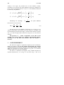
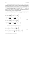
y
x
and ε 2
are the components of the potential
2
x +y
x + y2
εA created by an infinite string along the Oz axis. ε = 2φ is twice the
where
−ε
2
magnetic flux trapped in the string or in the solenoid (see Appendix and
Fig. 2)
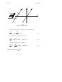
The electronic wave propagates from x = −∞ to x = +∞. The
"Young slits" are on a parallel to
x = −b .
Oy , at ±
a
from the point C located at
2
The potential appearing in (3) is a gradient because :
−
y
y
x
y
= ∂ x Arctg ; 2
= ∂ y Arctg
2
2
x +y
x x +y
x
2
so that the equation (3) is easily integrated, defining :
(4)
A new theory of the Aharonov-Bohm effect with a variant …
Σ = S − εArctg
533
y
x
(5)
which gives:
∂Σ  ∂Σ   ∂Σ 
2m
=  + 
∂t  ∂x   ∂y 
2
2
(6)
We choose the complete integral :
Σ = Et − 2 mE ( x cosθ o + y sin θ o )
(7)
Hence we get a complete integral of (3) :
S = Et − 2 mE ( x cosθ o + y sin θ o ) + ε Arctg
y
x
(8)
Or, in polar coordinates :
x = r cosθ , y = r sin θ
(9)
S = Et − 2 mE r cos(θ − θ o ) + ε θ
(10)
534
G. Lochak
y’
z
y
a/2
A+
x
-b
C
-a/2
O
A-
Fig. 2
Aharonov-Bohm scheme
The motion of the electron is given by the Jacobi theorem :
∂S
∂S
= Const ;
= Const
∂θ o
∂E
(11)
The trajectories are the rays of the wave :
∂S
= 2 mE ( x sin θ o − y cosθ o ) = µ
∂θ o
(12)
The motion along the rays is given by :
m
∂S
=t−
( x cosθ o + y sin θ o ) = to
2E
∂E
that is to say, with
E=
1 2
mv :
2
(13)
A new theory of the Aharonov-Bohm effect with a variant …
535
x cosθ o + y sin θ o = v(t − to )
(14)
We see that the rays (electron trajectories) defined by (12) are
orthogonal to the moving planes (13), but they are not orthogonal to the
equal phase surfaces (8), (10) except far away from the magnetic string
( x → ∞) where the ε potential term becomes negligible.
Therefore, despite the presence of the potential, the electronic
trajectories remain rectilinear and are not deviated because there is no
magnetic field. The velocity v = Const is the one of the incident electrons
because of the conservation of energy.
+
−
But the diffraction of the waves through the holes A and A
creates, for the electron trajectories, an interval of possible angles θ o , among
which are the angles of the interference fringes, modified by the magnetic
potential.
So there is no deviation of the electrons, but only a deviation of
the angles of phase synchronization between the waves issued from A+
and A- because a fieldless potential can only change the phases, not
the trajectories.
This is the Aharonov-Bohm effect that we now have to calculate.
Let us first look at the orthogonal lines to the equal phase surfaces
S : they are enveloped by the Lagrange momenta i.e. by the de Broglie
wave-vectors, in accordance with the formula (1), while the rays (12) are the
impulse lines mv.
The momenta are :
px = −
∂S
y
= 2 mE cosθ o − ε 2
∂x
x + y2
(15)
∂S
x
py = −
= 2 mE sin θ o + ε 2
∂y
x + y2
Hence the equation :
dx
y
2 mE cosθ o − ε 2
x + y2
=
dy
2 mE sin θ o + ε
x
2
x + y2
(16)
536
G. Lochak
The integration is obvious thanks to the integral combinations
and xdy − ydx . In polar coordinates, we find :
r sin(θ − θ o ) − Λ log
r
= c ( = Const ) , Λ =
Λ
xdx + ydy
ε
2mE
(17)
and in Cartesian coordinates :
x 2 + y2
y cosθ o − x sin θ o − Λ log
=c
Λ
(18)
Comparing with (12), one can see that the orthogonal lines to the
phase planes become parallel to the rays, far from the magnetic string. It is
worth noting that phase orthogonal lines (17) or (18), and the phase velocity
V=
hν
(which we cannot calculate here because the frequency is correct
p
only in relativity) depends on the potential through the momentum p ; but
this is not the case for the electron trajectories (12) and for the electron
velocity in (14).
In other words, the electrons (i.e. energy) do not follow the phase
propagation, neither in velocity, nor in trajectory. The same happens in
crystal optics : the phase propagation depends on the inductions (that is on
the polarization of the medium), while the propagation of energy is given by
the Poynting vector, which is only defined by fields and does not depend on
the polarization [4].
The shifting of interference fringes.
Ox (θ o = 0) .The
+
holes A and A will emit in the half space x > 0 two waves S and
−
S . According to (8), we have :
Let us consider a plane wave propagating along
+
−
A new theory of the Aharonov-Bohm effect with a variant …
a 
y

S + = Et − 2 mE  x + b +  y −  θ o  + ε Arctg


x
2


a 
y

S = Et − 2 mE  x + b +  y +  θ o  + ε Arctg

x
2 

537
(19)
−
θ o : cosθ o ≈ 1,
sin θ o ≈ θ o . Let us now suppose that t = 0 when x = − b , and let us
where we have taken into account the smallness of
write :
ξ = Arctg
The initial waves S + and S -, in
a
2b
(20)
a
A + and A −  x = − b, y = ±  ,

2
are :
So+ = −εξ , So+ = +εξ
(21)
Now, let us note that, in all the known experiments, the magnetic
+
−
string, or the solenoid, was very close to A and A . The authors say :
« in the shadow » of the electrostatic fiber of the Möllenstedt biprism [2], as
+
−
it is shown on the Fig. 1. Therefore, in A and A , the distance b is
π
π +
π
−
, so that So = + ε , So = − ε , .
2
2
2
+
−
Therefore, we see that in A and A , at the beginning of the
very small and
ξ∝
trajectories, the phases defined by (21) depend on the potential exclusively
through the value of ε . On the contrary, at the other end of the trajectories,
+
−
on the interference fringes, far from A and A , the distance is of the order
−4
of 15cm , while a, b ∝ 10 cm , which justifies the approximation of
+
−
parallel trajectories for the waves S and S in the vicinity of the fringes.
Close to the fringes, the term εθ , in (8) and (10), has practically the
+
−
same value for S and S : θ is very small and εδθ would be of the
third order, so it disappears from (19). In other words, on the fringes,
538
G. Lochak
contrary to the origin, the potential has no more influence. Finally,
according to (19) and (20), the phase difference respectively undergone by
+
−
the two waves propagating from A and A to the interference field will
be defined by the quantities :
a 

S + − So+ = Et − 2 mE  x + b +  y −  θ o  + εξ

2 


S − S = Et − 2 mE  x + b +  y +


−
−
o
Introducing the wavelengh
λ=
a 
θ o − εξ
2  
(22)
h
, the phase difference
2 mE
between the two waves will be :
∆ϕ =
∆S aθ o 2εξ
=
+
h
λ
h
(23)
The first term gives the standard Young fringes, the second one is the
Aharonov-Bohm effect. The formula (23) is not exactly in accordance with
the classical theory because of the angle ξ which is absent from the classical
one. ξ is half the angle under which the Young slits are seen from the
solenoid.
The presence of ξ entails a dependence of the effect on the
position of the string, which is in principle experimentally testable :
according to (20) the effect must decrease when the distance b
increases.
3
A NEW EXPERIMENT
We shall now suggest an experiment inspired by that of AharonovBohm, but which is such that the circular integral along the electron
trajectories equals zero an thus cannot have any relation with the fringe
shift. This experiment was already suggested in [6] but as an intuitive
argument. Here we give the exact calculation.
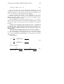
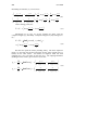
The idea is to substitute the magnetic string included between the
electronic trajectories by two strings on both sides (Fig. 3 and 4). In
A new theory of the Aharonov-Bohm effect with a variant …
539
principle, one string would be enough, but we shall see that the effect is
smaller than Aharonov-Bohm's, so that it is useful to double it. Owing to
the new position of strings, the magnetic flux through the closed line of
trajectories will be equal to zero because the potential is still a gradient and
its source is outside. The effect remains, but the problem of gauge invariance
is clearly irrelevant.
The Hamilton-Jacobi equation becomes here :
2m


∂S  ∂S
y−c
y+c
=  +ε 2
2 + 2
2  +
∂t  ∂x
x + ( y + c)  
 x + ( y − c)
 ∂S


x
x
+ − ε  2
2 + 2
2 
x + ( y + c)  
 x + ( y − c)
 ∂y
(24)
We see that, according to Fig. 3 and 4, the magnetic strings are parallel to
Oz , and cut the plane xOz in two points at a distance c from Oz. We
suppose :
c>
a
2
(25)
in order to put the strings outside the trajectories.
Fresnel- Möllenstedt biprism
solenoids
S
1
2
++
++ ++
+
h k = p = mv - eA
h k = p = mv + eA
Fig. 3
New experiment
F
540
G. Lochak
Paralleling the relations (4), we now have :

 ∂
y−c
y+c
y−c ∂
y+c
Arctg
Arctg
− 2
+
2 + 2
2 =
x
x
∂x
x + ( y + c)  ∂x
 x + ( y − c)

 ∂
x
x
y−c ∂
y+c
 x 2 + y − c 2 + x 2 + y + c 2  = ∂y Arctg x + ∂y Arctg x
(
)
(
)

(26)
And in analogy with (24) :
y−c
y + c
Σ = S − ε  Arctg
+ Arctg

x
x 
(27)
Introducing (27) in (24), we get the equation (6) again, with the
complete integral (7), and finally a complete integral of (24), analogous to
(8) :
S = Et − 2 mE ( x cosθ o + y sin θ o ) +
y−c
y + c
+ε  Arctg
+ Arctg

x
x 
(28)
We shall not repeat the whole preceding theory. The most important
thing is to note that the electron trajectories are the same straight lines as
before, for the same reason : the absence of magnetic field. We find
equations (12), (13), (14) again, for the wave rays. The Lagrange momenta
(de Broglie wave vectors, up to a factor h ) are now :
px = −


∂S
y−c
y+c
= 2 mE cosθ o − ε  2
2 + 2
2
∂x
x + ( y + c) 
 x + ( y − c)


∂S
x
x
= 2 mE sin θ o + ε  2
py = −
2 + 2
2
∂y
x + ( y + c) 
 x + ( y − c)
(29)
A new theory of the Aharonov-Bohm effect with a variant …
541
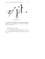
z
y’
y
c
a/2
A+
x
-b
C
-a/2
A-
O
-c
Fig. 4
New experiment scheme
The equations of the orthogonal lines of phase would be useless for the
prediction of the physical effect : it was interesting to perform the
integration only once, on the example (16), in order to show the difference
between rays and phase lines.
The shifting of interference fringes.
Let us look once more at a plane wave coming from x = −∞ to the
+
−
plane x = − b , and diffracting through the holes A and A . The angle
θ o is small again and we have, owing to (28) and in analogy with (19),
two waves :
542
G. Lochak
a 

S ± = Et − 2 mE  x + b +  y m  θ o  +

2 

y−c
y + c
+ ε  Arctg
+ Arctg

x
x 
(30)
For we have, up to a common constant additive term :
So+ = ε (η − ζ ) , So− = −ε (η − ζ )
(31)
with the definitions :
a
a
c+
2 ; ζ = Arctg
2
η = Arctg
b
b
c−
(32)
Disregarding, as in (19), the small terms corresponding to the potential
near the interference field (great values of x), we find the analogue of (22) for
+
−
the phase differences for the waves coming from A and A :
a 

S + − So+ = Et − 2 mE  x + b +  y −  θ o  − ε (η − ζ )

2 

a 

S − S = Et − 2 mE  x + b +  y +  θ o  + ε (η − ζ )

2 

−
(33)
−
o
Introducing the wavelength
λ=
h
, we can deduce the phase
2 mE
difference between the two waves, just as in (23) :
∆ϕ =
∆S aθ o 2ε
=
+ (ζ − η)
λ
h
h
(34)
We again find a first term, corresponding to the Young interferences,
and a second one analogous to the Aharonov-Bohm effect. This term is
smaller, for the obvious reason that each magnetic string produces a shift on
the nearest trajectory, but unfortunately it also produces a shift on the other
A new theory of the Aharonov-Bohm effect with a variant …
543
one, and this second shift is in the same direction as the first one because
both trajectories are on the same side of the string, whereas they were on
opposite sides in the case of Aharonov-Bohm, so that the phase shifts on the
trajectories were opposite too. This is why we find now, instead of a factor
ξ , the difference ζ − η , with η , ζ > 0 because we have chosen
(
)
a
in order for the string to be outside the trajectories. Nevertheless, the
2
c>
first shift dominates because the second trajectory is farther from the string
than the first one, so that the effect does exist. And since we have two
strings, the effect is doubled : hence the factor two before ε in (34).
Let us take, as an example, c = a . Then we have :
η = Arctg
a
3a
, ζ = Arctg
⇒ max(ζ − η) = 0, 52
2b
2b
The maximum value of
(ζ − η)
is obtained for
(35)
b=a
3
.
2
Comparing the maximum value of the Aharonov-Bohm shift in (20) :
ξ∝
π
≈ 1, 57 with the maximum shift in (34) : (ζ − η) ≈ 0, 52 , we see
2
that the effect predicted here is three times smaller. But this is not important
because the aim was not to give another proof of the interference shift due to
a fieldless potential (the Aharonov-Bohm proof is excellent), but to prove
that an effect of the same type can be obtained with an experiment which
cannot be explained in terms of a line integral which here obviously
vanishes.
4
THE QUESTION OF GAUGE INVARIANCE.
There is only one problem in an interference phenomenon : where are
the fringes ? And the answer is given by the phase difference between two
waves coming from two coherent sources.
Curiously, the calculation of this phase difference is at the basis of all
the interference phenomena except the Aharonov-Bohm effect ! The
interference is taken for granted and the only question is to find the
shift without damaging the gauge invariance. This is why the circular
integral of A plays the central role. But circular integral cannot give the
interfringe.
544
G. Lochak
Therefore, the phenomenon is calculated in two parts : a) The « free »
interference without potential. b) The shift due to the potential, considered
separately and which is absent from the calculation of the phase differences,
thus forgetting the geometry of the experiment. It is for this reason that the
location of the solenoid and the form under which the potential enters the
expression of the phase are forgotten.
If there is something new in the present paper, it is precisely an
attempt to come back to the old problems and methods of interference
phenomena owing to a simple calculation of phases.
Now we shall go back to the phases given by formulae (30), which
include the case of (19), adding in an arbitrary gauge term f ( x , y ) . We
find :
a 

S + = Et − 2 mE  x + b +  y −  θ o 

2 

y−c
y+c
+ε  Arctg
+ Arctg
+ f ( x , y + c)


x
x
a 

S = Et − 2 mE  x + b +  y +  θ o 

2 

y−c
y+c
+ε  Arctg
+ Arctg
+ f ( x , y − c)


x
x
(36)
−
Close to the slits, we have, generalizing (31) :
a
a


So+ = ε η − ζ + f  − c + f  + c 




2
2



 a

 a

S = ε − (η − ζ ) + f − + c  + f − − c 

 
 2
 2

−
o
and the phase difference (34) becomes :
(37)
A new theory of the Aharonov-Bohm effect with a variant …
545
a

 a 
− c + f  + c
f






2
2
2ε
2ε
aθ
 (38)
∆ϕ = o +
(η − ζ ) + 
λ
h
h    a 
  a  
 − f  −  2 + c  − f  −  2 − c  



 
Clearly, except if f ( x , y ) is even in y , the phase difference is
modified and that the phenomenon is not gauge invariant.
5
APPENDIX. The magnetic potential of an infinetely
thin and long solenoid or an infinite magnetic string.
We start from a classical formula in electromagnetism [8], [9],
expressing the vector potential created by a magnetic dipole µ at a distance
l:
A=
In a point
µ×l
l3
(39)
P , the potential is equal to :
+∞
+∞
dZ × l
dZ × MP
A=φ ∫
=φ ∫
3
3
l
MP
−∞
−∞
(40)
φ is the magnetic flux trapped in the string or in the solenoid, and :
MP 2 = l 2 = x 2 + y 2 + ( z − Z )
dZ × MP = {− y dZ , x dZ , 0}
Now we get from (40) :
2
(41)
546
G. Lochak
+∞
Ax = − φ y
∫ [x
−∞
+∞
Ay = φ x
∫[
−∞
2
dz
2
+ y + (z − Z )
]
2
dz
2
2
2
x + y + (z − Z )
]
3/ 2
3/ 2
(42)
; Az = 0
and given that :
+∞
∫ [x
−∞
2
dz
2
+ y + (z − Z )
2
]
3/ 2
=
2
x + y2
2
(43)
we find :
Ax = − 2 φ
y
x
; Ay = 2 φ 2
; Az = 0
2
x +y
x + y2
2
(44)
Acknowledgements :
I would like to dedicate this attempt to understand a little better these
difficult questions, to my old master Louis de Broglie and to David Bohm
with whom I worked in Paris at the Institute Henri Poincaré and who was a
friend of mine. Let them be postumously thanked for their teaching.
And I would like to thank warmly my son Pierre Lochak whose
valuable advice was for me of a great help. Of course, if all that is true, the
merit is shared, if it is not, the failure is mine.
Bibliography :
[1] Aharonov Y., Bohm D., Physical Review, 115, 485, 1959.
[2] Olariu S., Iovitsu Popescu I., Reviews of Modern Physics, 57, n°2,
1985, p. 339-436.
A new theory of the Aharonov-Bohm effect with a variant …
547
[3]Tonomura A.1, The Quantum World Unveiled by Electron Waves,
with a Preface of Chen Ning Yang, World Scientific, Singapore, 1998.
[4] Born M., Wolf E., Principles of Optics, Pergamon, Oxford, 1964.
[5] Broglie L. de, Thèse de 1924, Ann. Fond. Louis de Broglie, 17,
1992, p. 1-108.
[6] The Feynman Lectures in Physics, Vol. 2 Electrodynamics, AddisonWesley, 1964.
[7] Lochak G., Ann. Fond. Louis de Broglie, 25, 2000, p. 107-127.
[8] Tamm, I. E., Osnovy Teorii Electrichestva, OGIZ, Moscou, 1946.
[9] Jackson J. D., Classical Electrodynamics, 2nd ed., Wiley, N.Y., 1975.
(Manuscrit reçu le 11 février 2002, révisé le 20 septembre 2002)
1 The book of Akira Tonomura, written in non-technical terms, is in
principle, a popular book, but it is clear and profound and I highly
appreciate it, even if I can disagree with him on some points concerning
gauge invariance.