1
User’s Guide for Gappa
Guillaume Melquiond
User’s Guide for Gappa
by Guillaume Melquiond
Table of Contents
1. Introduction..................................................................................................................................... 1
2. Invoking Gappa............................................................................................................................... 2
2.1. Input and output ................................................................................................................... 2
2.2. Command-line options ......................................................................................................... 2
2.2.1. Selecting a proof back-end ...................................................................................... 2
2.2.1.1. Null back-end.............................................................................................. 2
2.2.1.2. Coq back-end .............................................................................................. 2
2.2.1.3. HOL Light back-end ................................................................................... 2
2.2.1.4. Coq back-end .............................................................................................. 3
2.2.2. Setting internal parameters ...................................................................................... 3
2.2.2.1. Internal precision ........................................................................................ 3
2.2.2.2. Dichotomy depth......................................................................................... 3
2.2.2.3. Fused multiply-add format.......................................................................... 3
2.2.3. Setting modes .......................................................................................................... 3
2.2.3.1. Assuming vague hypotheses ....................................................................... 3
2.2.3.2. Improving generated proofs ........................................................................ 4
2.2.3.3. Gathering statistics...................................................................................... 4
2.2.4. Enabling and disabling warning messages .............................................................. 4
2.3. Embedded options................................................................................................................ 5
3. Formalizing a problem ................................................................................................................... 6
3.1. Sections of a Gappa script.................................................................................................... 6
3.1.1. Logical formula ....................................................................................................... 6
3.1.1.1. Inequalities.................................................................................................. 6
3.1.1.2. Relative errors ............................................................................................. 7
3.1.2. Definitions ............................................................................................................... 7
3.1.3. Hints ........................................................................................................................ 8
3.2. Preferred expressions and other tricks ................................................................................. 8
3.2.1. Absolute and relative errors..................................................................................... 8
3.2.2. Global errors............................................................................................................ 8
3.2.3. Subsets of real numbers........................................................................................... 8
3.2.4. Disjunction .............................................................................................................. 9
3.3. Providing hints ..................................................................................................................... 9
3.3.1. Rewriting rules ........................................................................................................ 9
3.3.2. Approximated expressions .................................................................................... 10
3.3.3. Dichotomy search.................................................................................................. 10
4. Rounding operators ...................................................................................................................... 12
4.1. Rounding directions ........................................................................................................... 12
4.2. Floating-point operators ..................................................................................................... 12
4.3. Fixed-point operators ......................................................................................................... 13
4.4. Miscellaneous operators..................................................................................................... 13
4.4.1. Functions with relative error.................................................................................. 13
4.4.2. Rounding operators with homogen properties ...................................................... 14
5. Examples........................................................................................................................................ 15
5.1. A simple example to start from: x * (1 - x)........................................................................ 15
5.1.1. The C program....................................................................................................... 15
5.1.2. First Gappa version................................................................................................ 15
5.1.3. Defining notations ................................................................................................. 15
5.1.4. Complete version................................................................................................... 16
iii
5.1.4.1. Notations ................................................................................................... 16
5.1.4.2. Logical formulas and numbers.................................................................. 17
5.1.4.3. Hints.......................................................................................................... 17
5.1.4.4. Full listing ................................................................................................. 17
5.2. Tang’s exponential function ............................................................................................... 18
5.2.1. The algorithm ........................................................................................................ 18
5.2.2. Gappa description.................................................................................................. 18
5.2.3. Full listing.............................................................................................................. 19
5.3. Fixed-point Newton division.............................................................................................. 20
5.3.1. The algorithm and its verification.......................................................................... 20
5.3.2. Adding hints .......................................................................................................... 20
5.3.3. Full listing 1........................................................................................................... 21
5.3.4. Improving the rewriting rules ................................................................................ 21
5.3.5. Full listing 2........................................................................................................... 22
6. Customizing Gappa ...................................................................................................................... 23
6.1. Defining a new back-end.................................................................................................... 23
6.2. Defining new rounding operators....................................................................................... 23
6.2.1. Function classes..................................................................................................... 23
6.2.2. Function generators ............................................................................................... 24
A. Gappa language............................................................................................................................ 26
A.1. Comments and embedded options .................................................................................... 26
A.2. Tokens and operator priority ............................................................................................. 26
A.3. Grammar ........................................................................................................................... 26
A.4. Logical formulas ............................................................................................................... 28
A.4.1. Undecidability ...................................................................................................... 28
A.4.2. Expressiveness ...................................................................................................... 28
B. Warning and error messages....................................................................................................... 29
B.1. Syntax error messages ....................................................................................................... 29
B.1.1. Error: $bison at line $17 column $42. .................................................................. 29
B.1.2. Error: unrecognized option ’$titi’. ........................................................................ 29
B.1.3. Error: the symbol $toto is redefined... .................................................................. 29
B.1.4. Error: $toto is not a rounding operator.................................................................. 29
B.1.5. Error: invalid parameters for $toto........................................................................ 29
B.1.6. Error: incorrect number of arguments when calling $toto.................................... 30
B.2. Error messages .................................................................................................................. 30
B.2.1. Error: undefined intervals are restricted to conclusions........................................ 30
B.2.2. Error: the range of $toto is an empty interval. ...................................................... 30
B.2.3. Error: a zero appears as a denominator in a rewriting rule. .................................. 30
B.3. Warning messages ............................................................................................................. 31
B.3.1. Warning: the hypotheses on $toto are trivially contradictory, skipping. .............. 31
B.3.2. Warning: $toto is being renamed to $titi............................................................... 31
B.3.3. Warning: although present in a quotient, the expression $toto may not have been
tested for non-zeroness. ......................................................................................... 31
B.3.4. Warning: $toto and $titi are not trivially equal. .................................................... 31
B.3.5. Warning: $titi is a variable without definition, yet it is unbound.......................... 32
B.4. Warning messages during proof computation ................................................................... 32
B.4.1. Warning: no path was found for $toto. ................................................................. 32
B.4.2. Warning: hypotheses are in contradiction, any result is true. ............................... 32
B.4.3. Warning: no contradiction was found. .................................................................. 32
B.4.4. Warning: some enclosures were not satisfied. ...................................................... 33
iv
B.4.5. Warning: when $toto is in $i1, $titi is in $i2 potentially outside of $i3. .............. 33
B.4.6. Warning: case split on $toto has not produced any interesting new result. .......... 33
B.4.7. Warning: case split on $toto has no range to split. ............................................... 34
B.4.8. Warning: case split on $toto is not goal-driven anymore...................................... 34
v
Chapter 1. Introduction
Gappa (Génération Automatique de Preuves de Propriétés Arithmétiques — automatic proof generation of arithmetic properties) is a tool intended to help verifying and formally proving properties on
numerical programs and circuits handling floating-point or fixed-point arithmetic.
This tool manipulates logical formulas stating the enclosures of expressions in some intervals. For
example, a formal proof of the property
c ∈ [−0.3, −0.1] ∧ (2a ∈ [3, 4] → b + c ∈ [1, 2]) ∧ a − c ∈ [1.9, 2.05]
→
b + 1 ∈ [2, 3.5]
can be generated thanks to the following Gappa script.
{
c in [-0.3,-0.1] /\
(2 * a in [3,4] -> b + c in [1,2]) /\
a - c in [1.9,2.05]
-> b + 1 in [2,3.5]
}
a -> a - c + c;
b -> b + c - c;
Through the use of rounding operators as part of the expressions, Gappa is specially designed to
deal with formulas that could appear when certifying numerical codes. In particular, Gappa makes it
simple to bound computational errors due to floating-point arithmetic.
1
Chapter 2. Invoking Gappa
2.1. Input and output
Gappa reads the script whose filename is passed as an argument to the tool, or on its standard input if
none. Such a script is made of three parts: the definitions, the logical formula, and the hints. Warning
messages, error messages, and results, are displayed on the standard error output. Gappa also sends to
the standard output a formal proof of the logical formula; its format depends on the selected back-end.
Finally, if the tool was unable to prove some goals, its return code is a nonzero value.
For example, the following command lines create a simple script in file test.g, pass it to Gappa, and
store the generated Coq proof in file test.v file. They also test the return code of Gappa and send the
generated proof to Coq so that it is automatically checked. Since the proof checker does not display
anything, it means no errors were detected and the result computed by Gappa is correct.
$ echo "{ x in [-2,2] -> x * x in ? }" > test.g
$ gappa -Bcoq test.g > test.v
Results for x in [-2, 2]:
x * x in [0, 1b2 {4, 2^(2)}]
$ echo "Return code is $?"
Return code is 0
$ coqc -I path/to/gappalib-coq test.v
$
2.2. Command-line options
2.2.1. Selecting a proof back-end
These options are mutually exclusive and cannot be embedded into scripts.
2.2.1.1. Null back-end.
Option: -Bnull
Do not enable any back-end. This is the default behavior. This is also the only back-end compatible
with the -Munconstrained option.
2.2.1.2. Coq back-end
Option: -Bcoq
When this back-end is selected, Gappa generates a script that proves the results it displays. This
script can be automatically verified by the Coq proof-checker. It can also be reused in bigger formal
developments made with Coq.
2
Chapter 2. Invoking Gappa
2.2.1.3. HOL Light back-end
Option: -Bholl
Similar to the previous option, but for the HOL Light proof-checker.
2.2.1.4. Coq back-end
Option: -Bcoq-lambda
This back-end is used by the gappa tactic available for the Coq proof checker. It generates a lambdaterm that can be directly loaded by the proof checker, but it only supports the features needed by the
tactic: no bisection nor rewriting.
2.2.2. Setting internal parameters
2.2.2.1. Internal precision
Option: -Eprecision=integer
This option sets the internal MPFR precision that Gappa uses when computing bounds of intervals.
The default value is 60 and should be sufficient for most uses.
2.2.2.2. Dichotomy depth
Option: -Edichotomy=integer
This option limits the depth of a dichotomy split. The default value is 100. It means that an interval
of width 1 is potentially split into 2100 intervals of width 2−100 relatively to the original interval. This
should be sufficient for most uses too.
2.2.2.3. Fused multiply-add format
Option: -E[no-]reverted-fma
By default (-Eno-reverted-fma), the expression fma(a,b,c) is interpreted as a * b + c. As this
may not be the preferred order for the operands, the option makes Gappa use c + a * b instead.
2.2.3. Setting modes
These options cannot be embedded into scripts.
2.2.3.1. Assuming vague hypotheses
Option: -Munconstrained
By default, Gappa checks that all its hypotheses hold before using a theorem. This mode weakens
the engine by making it skip hypotheses that are not needed for computing intermediate results. For
example, Gappa will no longer check that x is not zero before applying the lemma proving x / x in
[1,1].
3
Chapter 2. Invoking Gappa
This mode is especially useful when starting a proof on relative errors, as it makes it possible to get
some early results about them without having to prove that they are well-defined.
At the end of its run, Gappa displays all the facts that are left unproven. In the following example, the
property NZR indicates that Gappa possibly need to prove that a value (namely x - 1, which appears
as a denominator and is equal to zero for x equal to 1) is nonzero.
{ x in [1,2] ->
(x + 1) / (x + 1) in ? /\ (x - 1) / (x - 1) in ? }
Results for x in [1, 2]:
(x + 1) / (x + 1) in [1, 1]
(x - 1) / (x - 1) in [1, 1]
Unproven assumptions:
NZR(x - 1)
While Gappa only displays the properties that are left unproven at the end of its run, it may contain
false positive. This is especially true when one of the unproven properties actually relies on the proof
of another one. Both will be displayed as unproven, although only the second one needs to be proved.
This mode cannot be used when a proof back-end is selected, as a generated proof would contain
holes.
2.2.3.2. Improving generated proofs
Option: -Mexpensive
In this mode, Gappa tries to find shorter proofs. Although this mode may considerably slow down the
computations, its effectiveness is unfortunately far from being guaranteed.
2.2.3.3. Gathering statistics
Option: -Mstatistics
At the end of its computations, Gappa displays some statistics. For example, the second script of this
example gives:
Statistics:
4949 expressions were considered,
but then 0 of these got discarded.
14747 theorems were tried. Among these,
5963 were successfully instantiated,
yet 3247 of these were not good enough
and 2 were only partially better.
The first two lines show the amounts of intermediate expressions Gappa prepared. The first number is
the amount of expressions that were considered, and the second number is the amount of expressions
for which Gappa had not found any usable theorem. Once this set of expressions is ready, Gappa tries
to find properties by applying theorems. The next statistics count these theorems. First, the amount of
theorems Gappa tried to apply. Then, among the theorems for which Gappa could satisfy hypotheses,
some gave a usable result, and some others did not (because a better property was already proved at
the time the theorem was considered).
4
Chapter 2. Invoking Gappa
2.2.4. Enabling and disabling warning messages
By default, all the warning messages are enabled. See annex for details on warning messages during
parsing and during computations.
2.3. Embedded options
Options setting internal parameters or enabling warning messages can be embedded in a Gappa proof
script. It is especially important when the logical property cannot be proved with the default parameters. These options are passed through a special comment syntax: #@ -Edichotomy=200.
5
Chapter 3. Formalizing a problem
3.1. Sections of a Gappa script
A Gappa script contains three parts. The first one is used to give names to some expressions in order
to simplify the writing of the next parts. The second one is the logical formula one wants to prove
with the tool. The third one gives some hints to Gappa on how to prove it.
The following script shows these three parts on the first example.
# some notations for making the script readable
@rnd = float< ieee_32, ne >;
x = rnd(xx);
y rnd= x * (1 - x);
z = x * (1 - x);
# the logical formula that Gappa will try (and succeed) to prove
{ x in [0,1] -> y in [0,0.25] /\ y - z in [-3b-27,3b-27] }
#
z
y
y
three hints to help Gappa finding the proof
-> 0.25 - (x - 0.5) * (x - 0.5);
$ x;
- z $ x;
3.1.1. Logical formula
This is the fundamental part of the script, it contains the logical formula Gappa is expected to prove.
This formula is written between brackets and can contain any implication, disjunction, conjunction
of enclosures of mathematical expressions. Enclosures are either bounded ranges or inequalities. Any
identifier without definition is assumed to be universally quantified over the set of real numbers.
{ x - 2 in [-2,0] /\ (x + 1 in [0,2] -> y in [3,4]) -> not x <= 1 \/ x + y in ? }
The logical formula is first modified and loosely broken according to the rules of sequent calculus.
Each of the new formulas will then be verified by Gappa. Ranges on the right of these sub-formulas
can be left unspecified. Gappa will then suggest a range such that the logical formula is verified.
(1)
(2)
x <= 1 /\ x - 2 in [-2,0] -> x + 1 in [0,2] \/ x + y in ?
x <= 1 /\ x - 2 in [-2,0] /\ y in [3,4] -> x + y in ?
3.1.1.1. Inequalities
Inequalities can be used instead of enclosures. The tool will display them as intervals with an infinite
bound.
They can be present on both sides of a sub-formula. On the left, it will be used only if Gappa is already
able to compute an enclosure of the expression by another way.
On the right, Gappa will put a reverted copy on the left in order to increase the number of available
hypotheses, if the equality was part of a disjunction at top level.
For instance, given the first formula below, Gappa actually tries to prove the second one.
(before)
(after)
a <= 1 /\ b in [2,3] -> ((c >= 4 \/ d in [5,6]) /\ e in [7,8]) \/ f <= 9
a <= 1 /\ b in [2,3] /\ f >= 9 -> ((c >= 4 \/ d in [5,6]) /\ e in [7,8]) \/ f <= 9
In particular, when displaying the results, the tool will display the new hypothesis on f:
6
Chapter 3. Formalizing a problem
Results for a in [-inf, 1] and b in [2, 3] and f in [9, inf]:
Inequalities that give an upper bound on an absolute value are treated differently. They are assumed
to be full enclosures with a lower bound equal to zero. In other words, |x| <= 1 is syntactic sugar
for |x| in [0,1].
3.1.1.2. Relative errors
The relative error between an approximate value x and a more precise value y is expressed by (x y) / y. For instance, when one wants to prove a bound on it, one can write:
{ ... -> |(x - y) / y| <= 0x1p-53 }
However, this bound can only be obtained if y is (proved to be) nonzero. Similarly, if a hypothesis
was a bound on a relative error, this hypothesis would be usable by Gappa only if it can prove that its
denominator is nonzero.
Gappa provides another way of expressing relative errors which does not depend on the denominator
being nonzero. It cannot be used as a subexpression; it can only be used as the left-hand side of an
enclosure:
{ ... -> x -/ y in [-0x1p-53,0x1p-53] }
This enclosure on the relative error represents the following proposition: ∃ ∈ [−2−53 , 2−53 ], x =
y × (1 + ).
When the bounds on a relative error are symmetric, the enclosure can be written as |x -/ y| <=
... instead.
3.1.2. Definitions
Typing the whole expressions in the logical formula can soon become annoying and error-prone,
especially if they contain rounding operators. To ease this work, the user can define in another section
beforehand the expressions that will be used more than once. A special syntax also allows to avoid
embedding rounding operators everywhere.
First, rounding operators can be given a shorter name by using the @name =
definition<parameters> syntax. name can then be used wherever the whole definition would
have been used.
Next, common sub-terms of a mathematical expression can be shared by giving them a name with the
name = term syntax. This name can then be used in later definitions or in the logical formula or in
the hints. The equality itself does not hold any semantic meaning. Gappa will only use the name as
a shorter expression when displaying the sub-term, and in the generated proof instead of a randomly
generated name.
Finally, when all the arithmetic operations on the right side of a definition are followed by the same
rounding operator, this operator can be put once and for all on the left of the equal symbol. For
example, with the following script, Gappa will complain that y and z are two different names for the
same expression.
@rnd = float< ieee_32, ne>;
y = rnd(x * rnd(1 - x));
z rnd= x * (1 - x);
{ y - z >= 0 }
7
Chapter 3. Formalizing a problem
3.1.3. Hints
Hints for Gappa’s engine can be added in this last section, if the tool is not able to prove the logical
formula. These hints are either rewriting rules or bisection directives. Approximate and accurate expressions can also be provided in this section in order to generate lots of safe rewriting rules. Hints
will be described in depth later.
3.2. Preferred expressions and other tricks
Gappa rewrites expressions by matching them with well-known patterns. The enclosure of an unmatchable expression will necessarily have to be computed through interval arithmetic. As a consequence, to ensure that the expressions will benefit from as much rewriting as possible, special care
needs to be taken when expressing the computational errors.
3.2.1. Absolute and relative errors
Let exact be an arithmetic expression and approx an approximation of exact. The approximation
usually contains rounding operators while the exact expression does not. The absolute error between
these two expressions is their difference: approx - exact.
Writing the errors differently will prevent Gappa from applying theorems on rounding errors: -(x rnd(x)) may lead to a worse enclosure than rnd(x) - x.
The situation is similar for the relative error. It should be expressed as the quotient between the
absolute error and the exact value: (approx - exact) / exact. For enclosures of relative errors,
this is the same: approx -/ exact.
3.2.2. Global errors
The approx and exact expressions need to have a similar structure in order for the rewriting rules to
kick in. E.g., if exact is a sum of two terms a and b, then approx has to be the sum of two terms c
and d such that c and d are approximations of a and b respectively.
Indeed the rewriting rule for the absolute error of the addition is: (a + b) - (c + d) -> (a - c)
+ (b - d). Similarly, the rewriting rules for the multiplication keep the same ordering of sub-terms.
For example, one of the rules is: a * b - c * d -> (a - c) * b + c * (b - d). Therefore,
one should try not to mess with the structure of expressions.
If the two sides of an error expression happen to not have a similar structure, then a user rewriting rule
has to be added in order to put them in a suitable state. For instance, let us assume we are interested in
the absolute error between a and d, but they have dissimilar structures. Yet there are two expressions
b and c that are equal and with structures similar to a for b and d for c. Then we just have to add the
following hints to help Gappa:
b - c -> 0; # or "b-c in [0,0]" as a hypothesis
a ~ b; # a is an approximation of b
c ~ d; # c is an approximation of d
8
Chapter 3. Formalizing a problem
3.2.3. Subsets of real numbers
Checking in the logical formula that an expression is in a specific subset can be achieved by verifying that a rounding operator toward this subset is the identity for this expression. For example, to
check that e is an integer multiple of 2−17 , this property can be used: fixed<-17, dn>(e) - e in
[0,0]. Similarly, to test that only 17 bits are needed to represent this expression (assuming it is either
zero or no closer to zero than 2−2001 ): float<17, -2001, ne>(e) - e in [0,0].
When some terms are known to be in a particular subset, Gappa can be made aware of it by defining
these terms as rounded values of some other terms. For instance, if x is an integer between 5 and 15
by hypothesis, the formula can be written by introducing a dummy variable x_:
x = int<dn>(x_); # the rounding direction does not matter
{ x in [5,15] -> ... }
Note that Gappa is able to deduce from x in [7.1,8.6] that x (which is only a name for the
expression int<dn>(x_)) is actually equal to 7. In particular, asking Gappa to perform a dichotomy
on x will cause the tool to consider each integer value separately, if needed for the proof.
Finally, an expression may be known to take a few separate values, but not equally distributed. In
some particular cases, it may possible to use a complicated expression instead of a plain disjunction.
This prevents Gappa from separately considering all the branches. For instance, if x can take only the
three values 0, 2, and 17, one can write:
i
x
{
$
=
=
i
i
int<dn>(i_);
i * (19b-1 * i - 15b-1);
in [-1,1] -> ... }
in 3; # this dichotomy hint helps Gappa to understand that i is either -1, 0, or 1
3.2.4. Disjunction
When a formula contains a disjunction in its, one of the sides of this disjunction has to always hold
with respect to the set of hypotheses. This is especially important when performing dichotomies. Even
if Gappa is able to prove the formula in each particular branch of a dichotomy, if a different property
of the disjunction is used each time, the tool will fail to prove the formula in the general case.
3.3. Providing hints
3.3.1. Rewriting rules
Internally, Gappa tries to compute the range of mathematical terms. For example, if the tool has to
bound the product of two factors, it will check if it knows the ranges of both factors. If it does, it will
apply the theorem about real multiplication in order to compute the range of the product.
Unfortunately, there may be some expressions that Gappa cannot bound correctly. This usually happens because it has no result on a sub-term or because the expression is badly correlated. In this case,
the user can provide an alternate expression. If Gappa finds an enclosure for this secondary expression,
it will use its range in an enclosure for the primary expression.
primary -> secondary;
9
Chapter 3. Formalizing a problem
In order for this transformation to be valid, any evaluation of the primary expression must be contained
in the enclosure of the secondary expression. Gappa will generate the corresponding theorem in the
final proof script and its proof will be left as an exercise for the user.
This transformation is generally valid if both expressions are equal. To detect mistyping early, Gappa
will try to check if they are indeed equal and warn if they are not. It will not generate a proof of their
equality though and it is still up to the user to do it. Note that Gappa does not check if the divisor are
always different from zero in the expressions. Instead it warn about such potentially bad divisors.
The internal database of rules check for null divisors though. As a consequence, if a common rule
does not apply, this may mean that such a divisor exists. In order to test whether it is the case or
not, the -Munconstrained option allows to skip these checks. If Gappa is happy when this option is
provided, the input should be checked for null divisors. Note that this option obviously prevents the
proof generation.
3.3.2. Approximated expressions
As mentioned before, Gappa has an internal database of rewriting rules. Some of these rules need
to know about accurate and approximate terms. Without this information, they do not match any
expression. For example, Gappa will replace the term B by b + -(b - B) only it knows a term b
that is an approximation of the term B.
Gappa has two heuristics to detect terms that are approximations of other terms. First, rounded values
are approximations of their non-rounded counterparts. Second, any absolute or relative error that
appears as a hypothesis of a logical sub-formula will define a pair of accurate and approximate terms.
Since these pairs create lots of already proved rewriting rules, it is helpful for the user to define its
own pairs. This can be done with the following syntax.
approximate ~ accurate;
In the following example, the comments show two hints that could be added if they had not already
been guessed by Gappa. In particular, the second one enables a rewriting rule that completes the proof.
@floor = int<dn>;
{ x - y in [-0.1,0.1] -> floor(x) - y in ? }
# floor(x) ~ x;
# x ~ y;
3.3.3. Dichotomy search
The last kind of hint can be used when Gappa is unable to prove a formula but would be able to prove
it if the hypothesis ranges were not so wide. Such a failure is usually caused by a bad correlation
between the sub-terms of the expressions. This can be solved by rewriting the expressions. But the
failure can also happen when the proof of the formula is not the same everywhere on the domain, as
in the following example. In both cases, the user can ask Gappa to split the ranges into tighter ranges
and see if it helps proving the formula.
@rnd = float< ieee_32, ne >;
x = rnd(x_);
y = x - 1;
z = x * (rnd(y) - y);
{ x in [0,3] -> |z| in ? }
10
Chapter 3. Formalizing a problem
With this script, Gappa will answer that |z| ≤ 3·2−24 . This is not the best answer because Gappa does
not notice that rnd(y) - y is always zero when 12 ≤ x ≤ 3. The user needs to ask for a bisection
with respect to the expression rnd(x_).
There are three types of bisection. The first one splits an interval in as many equally wide sub-intervals
as asked by the user. The second one splits an interval along the points provided by the user.
$ x in 6;
# split the range of "x" in six sub-intervals
$ x in (0.5,1.9999999); # split the range of "x" in three sub-intervals, the middle one being [0.5,~2]
$ x;
# equivalent to: $ x in 4;
The third kind of bisection tries to find by dichotomy the best range split such that a goal of the logical
formula holds true. This requires the range of this goal to be specified, and the enclosed expression
has to be indicated on the left of the $ symbol.
{ x in [0,3] -> |z| <= 1b-26 }
|z| $ x;
Contrarily to the first two kinds of bisection, this third one keeps the range improvements only if the
goal was finally reached. If there was a failure in doing so, all the improvements are discarded. Gappa
will display the sub-range on which the goal was not proved. There is a failure when Gappa cannot
prove the goal on a range and this range cannot be split into two half ranges, either because its internal
precision is not enough anymore or because the maximum depth of dichotomy has been reached. This
depth can be set with the -Edichotomy=999 option.
More than one bisection hint can be used. And hints of the third kind can try to satisfy more than one
goal at once.
a, b, c $ u;
a, d $ v;
These two hints will be used one after the other. In particular, none will be used when Gappa is doing
a bisection with the other one. By adding terms on the right of the $ symbol, more complex hints can
be built. Beware of combinatorial explosions though. The following hint is an example of a complex
bisection: it asks Gappa to find a set of sub-ranges on u such that the goal on b is satisfied when the
range on v is split into three sub-intervals.
b $ u, v in 3
11
Chapter 4. Rounding operators
4.1. Rounding directions
Some of the classes of operators presented in the following sections are templated by a rounding direction. This is the direction chosen when converting a real number that cannot be exactly represented
in the destination format.
There are eleven directions:
zr
toward zero
aw
away from zero
dn
toward minus infinity (down)
up
toward plus infinity
od
to odd mantissas
ne
to nearest, tie breaking to even mantissas
no
to nearest, tie breaking to odd mantissas
nz
to nearest, tie breaking toward zero
na
to nearest, tie breaking away from zero
nd
to nearest, tie breaking toward minus infinity
nu
to nearest, tie breaking toward plus infinity
The rounding directions mandated by the IEEE-754 standard are ne (default mode, rounding to nearest), zr, dn, up, and na (introduced for decimal arithmetic).
12
Chapter 4. Rounding operators
4.2. Floating-point operators
This class of operators covers all the formats whose number sets are F (p, d) = {m × 2e ; |m| <
2p , e ≥ d}. In particular, IEEE-754 floating-point formats (with subnormal numbers) are part of this
class, if we set apart overflow issues. Both parameters p and d select a particular format. The last
parameter selects the rounding direction.
float< precision, minimum_exponent, rounding_direction >(...)
Having to remember the precision and minimum exponent parameters may be a bit tedious, so an
alternate syntax is provided: instead of these two parameters, a name can be given to the float class.
float< name, rounding_direction >(...)
There are four predefined formats:
ieee_32
IEEE-754 single precision
ieee_64
IEEE-754 double precision
ieee_128
IEEE-754 quadruple precision
x86_80
extended precision on x86-like processors
4.3. Fixed-point operators
This class of operators covers all the formats whose number sets are F (e) = {m × 2e }. The first
parameter selects the weight of the least significant bit. The second parameter selects the rounding
direction.
fixed< lsb_weight, rounding_direction >(...)
Rounding to integer is a special case of fixed point rounding of weight 0. A syntactic shortcut is
provided.
int< rounding_direction >(...)
4.4. Miscellaneous operators
4.4.1. Functions with relative error
This set of functions is defined with related theorems on relative error. They can be used to express
properties that cannot be directly expressed through unary rounding operators.
{add|sub|mul}_rel< precision [, minimum_exponent] >(..., ...)
13
Chapter 4. Rounding operators
If the minimum exponent is not provided, no domain will be excluded when considering the validity
of the theorems, not even zero. Otherwise the domain [−2e , 2e ] is excluded.
4.4.2. Rounding operators with homogen properties
To be written.
14
Chapter 5. Examples
5.1. A simple example to start from: x * (1 - x)
5.1.1. The C program
Let us analyze the following function.
float f(float x)
{
assert(0 <= x && x <= 1);
return x * (1 - x);
}
This function computes the value x * (1 - x) for an argument x between 0 and 1. The float type is
meant to force the compiler to use IEEE-754 single precision floating-point numbers. We also assume
that the default rounding mode is used: rounding to nearest number, break to even on tie.
The function returns the value x ⊗ (1 x) instead of the ideal value x · (1 − x) due to the limited
precision of the computations. If we rule out the overflow possibility (floating-point numbers are
limited, not only in precision, but also in range), the returned value is also ◦(x · ◦(1 − x)). This o
function is a unary operator related to the floating-point format and the rounding mode used for the
computations. This is the form Gappa works on.
5.1.2. First Gappa version
We first try to bound the result of the function. Knowing that x is in the interval [0,1], what is the
enclosing interval of the function result? It can be expressed as an implication: If x is in [0,1], then
the result is in ... something. Since we do not want to enforce some specific bounds yet, we use a
question mark instead of some explicit bounds.
The logical formula Gappa has to verify is enclosed between braces. The rounding operator is a
unary function float< ieee_32, ne >. The result of this function is a real number that would fit
in a IEEE-754 single precision (ieee_32) floating-point number (float), if there was no overflow.
This number is potentially a subnormal number and it was obtained by rounding the argument of the
rounding operator toward nearest even (ne).
The following Gappa script finds an interval such that the logical formula describing our previous
function is true.
{ x in [0,1] -> float<ieee_32,ne>(x * float<ieee_32,ne>(1 - x)) in ? }
Gappa answers that the result is between 0 and 1. Without any help from the user, they are the best
bounds Gappa is able to prove.
Results for x in [0, 1]:
[rounding_float,ne,24,149](x * [rounding_float,ne,24,149](1 - x)) in [0, 1]
15
Chapter 5. Examples
5.1.3. Defining notations
Directly writing the completely expanded logical formula is fine for small formulas, but it may become tedious once the problem gets big enough. For this reason, notations can be defined to avoid
repeating the same terms over and over. These notations are all written before the logical formula.
For example, if we want not only the resulting range of the function, but also the absolute error, we
need to write the expression twice. So we give it the name y.
y = float<ieee_32,ne>(x * float<ieee_32,ne>(1 - x));
{ x in [0,1] -> y in ? /\ y - x * (1 - x) in ? }
We can simplify the input a bit further by giving a name to the rounding operator too.
@rnd = float< ieee_32, ne >;
y = rnd(x * rnd(1 - x));
{ x in [0,1] -> y in ? /\ y - x * (1 - x) in ? }
These explicit rounding operators right in the middle of the expressions make it difficult to directly
express the initial C code. So we factor the operators by putting them before the equal sign.
@rnd = float< ieee_32, ne >;
y rnd= x * (1 - x);
{ x in [0,1] -> y in ? /\ y - x * (1 - x) in ? }
Please note that this implicit rounding operator only applies to the results of arithmetic operations. In
particular, a rnd= b is not equivalent to a = rnd(b). It is equivalent to a = b.
Finally, we can also give a name to the infinitely precise result of the function to clearly show that
both expressions have a similar arithmetic structure.
@rnd = float< ieee_32, ne >;
y rnd= x * (1 - x);
z = x * (1 - x);
{ x in [0,1] -> y in ? /\ y - z in ? }
On the script above, Gappa displays:
Results for x in [0, 1]:
y in [0, 1]
y - z in [-1b-24 {-5.96046e-08, -2^(-24)}, 1b-24 {5.96046e-08, 2^(-24)}]
Gappa displays the bounds it has computed. Numbers enclosed in braces are approximations of the
numbers on their left. These exact left numbers are written in decimal with a power-of-two exponent.
The precise format will be described below.
5.1.4. Complete version
Previously found bounds are not as tight as they could actually be. Let us see how to expand Gappa’s
search space in order for it to find better bounds. Not only Gappa will be able provide a proof of the
optimal bounds for the result of the function, but it will also prove a tight interval on the computational
absolute error.
5.1.4.1. Notations
x = rnd(xx);
y rnd= x * (1 - x);
z = x * (1 - x);
# x is a floating-point number
# equivalent to y = rnd(x * rnd(1 - x))
16
Chapter 5. Examples
The syntax for notations is simple. The left-hand-side identifier is a name representing the expression
on the right-hand side. Using one side or the other in the logical formula is strictly equivalent. Gappa
will use the defined identifier when displaying the results and generating the proofs though, in order
to improve their readability.
The second and third notations have already been presented. The first one defines x as the rounded
value of a real number xx. In the previous example, we had not expressed this property of x: it is a
floating-point number. This additional piece of information will help Gappa to improve the bound on
the error bound. Without it, a theorem like Sterbenz’ lemma cannot apply to the 1 - x subtraction.
5.1.4.2. Logical formulas and numbers
{ x in [0,1] -> y in [0,0.25] /\ y - z in [-3b-27,3b-27] }
Numbers and bounds can be written either in the usual scientific decimal notation or by using a powerof-two exponent: 3b-27 means 3 · 2−27 . Numbers can also be written with the C99 hexadecimal
notation: 0x0.Cp-25 is another way to express the bound on the absolute error.
5.1.4.3. Hints
Although we have given additional data through the type of x, Gappa is not yet able to prove the
formula. It needs some user hints.
z -> 0.25 - (x - 0.5) * (x - 0.5);
y $ x;
y - z $ x;
# x * (1 - x) == 1/4 - (x - 1/2)^2
# bound y by splitting the interval on x
# bound y - z by splitting ...
The first hint indicates to Gappa that both hand sides are equivalent: When it tries to bound the left
hand side, it can use the bounds it has found for the right hand side. Please note that this rewriting
only applies when Gappa tries to bound the expression, not when it tries to bound a bigger expression.
The two other hints indicate that Gappa should bound the left-hand-side values by doing a case split on
the right-hand side. It only works if the logical proposition requires explicit bounds for the expression
on the left hand side.
5.1.4.4. Full listing
As a conclusion, here is the full listing of this example.
# some notations
@rnd = float< ieee_32, ne >;
x = rnd(xx);
y rnd= x * (1 - x);
z = x * (1 - x);
# x is a floating-point number
# equivalent to y = rnd(x * rnd(1 - x))
# the value we want to approximate
# the logical property
{ x in [0,1] -> y in [0,0.25] /\ y - z in [-3b-27,3b-27] }
#
z
y
y
hints
-> 0.25 - (x - 0.5) * (x - 0.5);
$ x;
- z $ x;
# x * (1 - x) == 1/4 - (x - 1/2)^2
# bound y by splitting the interval on x
# bound y - z by splitting ...
Gappa gives the results below.
Warning: z and 25e-2 - (x - 5e-1) * (x - 5e-1) are not trivially equal.
Difference: (5e-1)^2 - (25e-2) - 2 * (x) * (5e-1) + (x)
17
Chapter 5. Examples
Results for x in [0, 1]:
y in [0, 1b-2 {0.25, 2^(-2)}]
y - z in [-3b-27 {-2.23517e-08, -2^(-25.415)}, 3b-27 {2.23517e-08, 2^(-25.415)}]
Note that Gappa checks the rewriting rules in order to provide early detection of mistyping. Since
this check does not involve computations on decimal numbers, Gappa warns about the user hint on
z. This false positive can be avoided by adding the special comment #@ -Wno-hint-difference
before the offending rule.
5.2. Tang’s exponential function
5.2.1. The algorithm
In Table-Driven Implementation of the Exponential Function in IEEE Floating-Point Arithmetic, Ping
Tak Peter Tang described an implementation of an almost correctly-rounded elementary function in
single and double precision. John Harrison later did a complete formal proof in HOL Light of the
implementation in Floating point verification in HOL Light: the exponential function.
Here we just focus on the tedious computation of the rounding error. We consider neither the argument
reduction nor the reconstruction part (trivial anyway, excepted when the end result is subnormal). We
want to prove that, in the C code below, the absolute error between e and the exponential E0 of R0
(the ideal reduced argument) is less than 0.54 ulp. Variable n is an integer and all the other variables
are single-precision floating-point numbers.
r2 = -n * l2;
r = r1 + r2;
q = r * r * (a1 + r * a2);
p = r1 + (r2 + q);
s = s1 + s2;
e = s1 + (s2 + s * p);
Let us note R the computed reduced argument and S the stored value of the ideal constant S0. There
1
are 32 such constants. For the sake of simplicity, we only consider the second constant: 2 32 . E is
the value of the expression e computed with an infinitely precise arithmetic. Z is the absolute error
2
between the polynomial x + a1 · x2 + a2 · x3 and exp(x) − 1 for |x| ≤ log
64 .
5.2.2. Gappa description
a1
a2
l2
s1
s2
=
=
=
=
=
8388676b-24;
11184876b-26;
12566158b-48;
8572288b-23;
13833605b-44;
r2 rnd= -n * l2;
r rnd= r1 + r2;
q rnd= r * r * (a1 + r * a2);
p rnd= r1 + (r2 + q);
s rnd= s1 + s2;
e rnd= s1 + (s2 + s * p);
R = r1 + r2;
S = s1 + s2;
E0 = S0 * (1 + R0 + a1 * R0 * R0 + a2 * R0 * R0 * R0 + Z);
18
Chapter 5. Examples
{ Z in [-55b-39,55b-39] /\ S - S0 in [-1b-41,1b-41] /\ R - R0 in [-1b-34,1b-34] /\
R in [0,0.0217] /\ n in [-10176,10176]
->
e in ? /\ e - E0 in ? }
Gappa is unable to bound the expressions. This is not surprising for e - E0, since the tool is missing
some of the implicit transformations hidden in the implementation. As for e itself, Gappa is missing
the range of r1. Since Gappa has access to the ranges of R and r2, this issue can be solved by adding
the hint: r1 -> R - r2.
Please note the way Z is introduced. Its definition is backward: Z is a real number such that E0 is the
product of S0 and the exponential of R0. It makes for clearer definitions and it avoids having to deal
with divisions.
Now to e - E0. We compute this error by splitting it between a pure rounding error e - E and
another term which combines discretization and truncation errors. This term is E - E0. Unfortunately,
Gappa is unable to compute tight bounds for this term since the syntactic structures of its sub-terms
do not match.
So we introduce a new expression Er equal to E yet matching the structure of E0. Since Z has no
equivalent term in E, we insert an artificial term 0 in the corresponding place in Er.
E = s1 + (s2 + S * (r1 + (r2 + R * R * (a1 + R * a2))));
Er = S * (1 + R + a1 * R * R + a2 * R * R * R + 0);
...
e - E0 -> (e - E) + (Er - E0);
5.2.3. Full listing
@rnd = float< ieee_32, ne >;
a1
a2
l2
s1
s2
=
=
=
=
=
8388676b-24;
11184876b-26;
12566158b-48;
8572288b-23;
13833605b-44;
r2 rnd= -n * l2;
r rnd= r1 + r2;
q rnd= r * r * (a1 + r * a2);
p rnd= r1 + (r2 + q);
s rnd= s1 + s2;
e rnd= s1 + (s2 + s * p);
R = r1 + r2;
S = s1 + s2;
E = s1 + (s2 + S * (r1 + (r2 + R * R * (a1 + R * a2))));
Er = S * (1 + R + a1 * R * R + a2 * R * R * R + 0);
E0 = S0 * (1 + R0 + a1 * R0 * R0 + a2 * R0 * R0 * R0 + Z);
{ Z in [-55b-39,55b-39] /\ S - S0 in [-1b-41,1b-41] /\ R - R0 in [-1b-34,1b-34] /\
R in [0,0.0217] /\ n in [-10176,10176] ->
e in ? /\ e - E0 in ? }
e - E0 -> (e - E) + (Er - E0);
r1 -> R - r2;
Gappa answers that the error is bounded by 0.535 ulp. This is consistent with the bounds computed
by Tang and Harrison.
19
Chapter 5. Examples
Results for n in [-10176, 10176] and R in [0, 0.0217] and Z in [-1.00044e-10, 1.00044e-10] and S - S0 in [4.54747e-13, 4.54747e-13] and R - R0 in [-5.82077e-11, 5.82077e-11]:
e in [4282253b-22 {1.02097, 2^(0.0299396)}, 8768135b-23 {1.04524, 2^(0.0638374)}]
e - E0 in [-75807082762648785b-80 {-6.27061e-08, -2^(-23.9268)}, 154166255364809243b-81 {6.37617e-08, 2^(23.9027)}]
5.3. Fixed-point Newton division
5.3.1. The algorithm and its verification
Let us suppose we want to invert a floating-point number on a processor without a floating-point unit.
The 24-bit mantissa has to be inverted from a value between 0.5 and 1 to a value between 1 and 2.
For the sake of this example, the transformation is performed by Newton’s iteration with fixed-point
arithmetic.
The mantissa is noted d and its exact reciprocal is R. Newton’s iteration is started with a first approximation r0 taken from a table containing reciprocals at precision ±2−8 . Two iterations are then
performed. The result r1 of the first iteration is computed on 16-bit words in order to speed up computations. The result r2 of the second iteration is computed on full 32-bit words. We want to prove
that this second result is close enough to the infinitely precise reciprocal R = 1/d.
First, we define R as the reciprocal, and d and r0 as two fixed-point numbers.
d = fixed<-24,dn>(d_);
R = 1 / d;
r0 = fixed<-8,dn>(r0_);
Next we have the two iterations. Gappa’s representation of fixed-point arithmetic is high-level: the tool
is only interested in the weight of the least significant bit. The shifts that occur in an implementation
only have an impact on the internal representation of the values, not on the values themselves, so
Gappa is only aware of them through the displacements of the least significant bits.
r1 fixed<-14,dn>= r0 * (2 - fixed<-16,dn>(d) * r0);
r2 fixed<-30,dn>= r1 * (2 - d * r1);
The property we are looking for expresses the absolute error between r2 and R, knowing that r0 is an
approximation of R and that d is bounded.
{ r0 - R in [-1b-8,1b-8] /\ d in [0.5,1] -> r2 - R in ? }
We expect Gappa to prove that r2 is R ± 2−24 . Unfortunately, this is not the case.
Results for d in [0.5, 1] and r0 - R in [-0.00390625, 0.00390625]:
r2 - R in [-1320985b-18 {-5.03916, -2^(2.33318)}, 42305669b-23 {5.04323, 2^(2.33435)}]
5.3.2. Adding hints
With the previous script, Gappa computes a range so wide for r2 - R that it is useless. This is not
surprising: The tool does not know what Newton’s iteration is. In particular, Gappa cannot guess that
such an iteration has a quadratic convergence. Testing for r1 - R instead does not give results any
better.
20
Chapter 5. Examples
Gappa does not find any useful relation between r1 and R, as the first one is a rounded multiplication
while the second is an exact division. So we have to split the absolute error into two terms: a rounding
error we expect Gappa to compute, and the convergence due to Newton’s iteration.
{ r0 - R in [-1b-8,1b-8] /\ d in [0.5,1] ->
r1 - r0 * (2 - d * r0) in ? /\ r0 * (2 - d * r0) - R in ? }
Gappa now gives the answer below. Notice that the range of the rounding error almost matches the
precision of the computations.
Results for d in [0.5, 1] and r0 - R in [-0.00390625, 0.00390625]:
r0 * (2 - d * r0) - R in [-131585b-16 {-2.00783, -2^(1.00564)}, 263425b-17 {2.00977, 2^(1.00703)}]
r1 - r0 * (2 - d * r0) in [-1b-14 {-6.10352e-05, -2^(-14)}, 788481b-32 {0.000183583, 2^(-12.4113)}]
So Gappa was fine with the rounding error, but not with the algorithmic error. We can help Gappa by
directly providing an expression of this error. So we add a rule describing the quadratic convergence
of Newton’s iteration. And since we also have to split r1 - R, we perform both operations in one
single rewriting rule.
r1 - R -> (r1 - r0 * (2 - d * r0)) - (r0 - R) * (r0 - R) * d;
A similar rule is then used for r2 - R.
5.3.3. Full listing 1
d = fixed<-24,dn>(d_);
R = 1 / d;
r0 = fixed<-8,dn>(r0_);
r1 fixed<-14,dn>= r0 * (2 - fixed<-16,dn>(d) * r0);
r2 fixed<-30,dn>= r1 * (2 - d * r1);
{ r0 - R in [-1b-8,1b-8] /\ d in [0.5,1] -> r2 - R in ? }
r1 - R -> (r1 - r0 * (2 - d * r0)) - (r0 - R) * (r0 - R) * d;
r2 - R -> (r2 - r1 * (2 - d * r1)) - (r1 - R) * (r1 - R) * d;
Gappa answers that r2 = R ± 2−24.7 .
Warning: although present in a quotient, the expression (d) may have not been tested for non-zeroness.
Results for d in [0.5, 1] and r0 - R in [-0.00390625, 0.00390625]:
r2 - R in [-639017422849b-64 {-3.46412e-08, -2^(-24.7829)}, 1541b-39 {2.80306e-09, 2^(-28.4103)}]
5.3.4. Improving the rewriting rules
First of all, there is this warning message about d possibly being zero. Indeed, R is the reciprocal of d
and we are using the fact that R * d = 1. So the rewriting rules cannot be proven on their own. As a
consequence, while the result is correct, its proof is flawed. In order to avoid this issue, we can give
the precise hypotheses such that the left hand sides of the rewriting rules are equal to their right hand
side. Here, Gappa just has to prove that d is not zero. This is indicated at the end of the rule.
r1 - R -> (r1 - r0 * (2 - d * r0)) - (r0 - R) * (r0 - R) * d
{d <> 0};
Second, the rewriting rules are too specialized. For example, in the first one, the occurrences of r1
could be replaced by any other real number and the rule would still be valid. Let us consider the
21
Chapter 5. Examples
problem again. We wanted to split r1 - R into a rounding error and an algorithmic error. So we
could just say that r1 is an approximation of r0 * (2 - d * r0).
r1 ~ r0 * (2 - d * r0);
We are left with hinting Gappa at the quadratic convergence of Newton’s iterations.
r0 * (2 - d * r0) - R -> (r0 - R) * (r0 - R) * -d
{ d <> 0};
When generating a script for an external proof checker, Gappa will add this rewriting rule as a global
hypothesis. For example, when selecting the Coq back-end with the option -Bcoq, the output contains
the line below.
Hypothesis a1 : (_d <> 0)%R -> r11 = r3.
In this hypothesis, _d is the d variable of the example, while r11 and r3 are short notations for
r0 * (2 - d * r0) - R and (r0 - R) * (r0 - R) * -d respectively. In order to access the
generated proof, the user has to prove this hypothesis, which can be trivially done with Coq’s field
tactic.
5.3.5. Full listing 2
d = fixed<-24,dn>(d_);
R = 1 / d;
r0 = fixed<-8,dn>(r0_);
r1 fixed<-14,dn>= r0 * (2 - fixed<-16,dn>(d) * r0);
r2 fixed<-30,dn>= r1 * (2 - d * r1);
{ r0 - R in [-1b-8,1b-8] /\ d in [0.5,1] -> r2 - R in ? }
r1
r0
r2
r1
~
*
~
*
r0
(2
r1
(2
*
*
-
(2 - d * r0);
d * r0) - R -> (r0 - R) * (r0 - R) * -d
(2 - d * r1);
d * r1) - R -> (r1 - R) * (r1 - R) * -d
{ d <> 0};
{ d <> 0};
The answer is the same.
Results for d in [0.5, 1] and r0 - R in [-0.00390625, 0.00390625]:
r2 - R in [-639017422849b-64 {-3.46412e-08, -2^(-24.7829)}, 1541b-39 {2.80306e-09, 2^(-28.4103)}]
22
Chapter 6. Customizing Gappa
These sections explain how rounding operators and back-ends are defined in the tool. They are
meant for developers rather than users of Gappa and involve manipulating C++ classes defined in
the src/arithmetic and src/backends directories.
6.1. Defining a new back-end
To be written.
6.2. Defining new rounding operators
6.2.1. Function classes
A function derives from the function_class class. This class is an interface to the name of the
function, its associated real operator, and six theorems.
struct function_class {
real_op_type type;
int theorem_mask;
function_class(real_op_type t, int m): type(t), theorem_mask(m) {}
virtual std::string name() const = 0;
virtual interval round
(interval const &, std::string
virtual interval enforce
(interval const &, std::string
virtual interval absolute_error
(std::string
virtual interval absolute_error_from_real
(interval const &, std::string
virtual interval absolute_error_from_rounded(interval const &, std::string
virtual interval relative_error_from_real
(interval const &, std::string
virtual interval relative_error_from_rounded(interval const &, std::string
virtual ~function_class() {}
};
&)
&)
&)
&)
&)
&)
&)
const;
const;
const;
const;
const;
const;
const;
The name is a string given through the virtual method name. It will be used when generating the
notations of the proof. If the description of the final function needs more than a name, additional
parameters can be provided by adding them to the name after a comma. The back-end will take
care of the formatting of the final string. This remark also applies to names returned by the theorem
methods (see below).
The type is the associated real operator. This will be UOP_ID (the unary identity function) for standard
rounding operators. But it can be more complex if needed:
enum real_op_type { UOP_ID, UOP_NEG, UOP_ABS, BOP_ADD, BOP_SUB, BOP_MUL, BOP_DIV, ... };
The type will indicate to the parser the number of arguments the function requires. For example, if
the BOP_DIAM type is associated to the function f, then f will be parsed as a binary function. But the
type is also used by the rewriting engines in order to derive default rules for this function. These rules
involve the associated real operator (the diamond in this example).
f (a, b) − c d
f (a, b) − c d
cd
−→
−→
(f (a, b) − a b) + (a b − c d)
f (a, b) − a b a b − c d f (a, b) − a b a b − c d
+
+
·
ab
cd
ab
cd
23
Chapter 6. Customizing Gappa
For these rules and the following theorems to be useful, the expressions f (a, b) and a b have to be
close to zero. Bounding their distance is the purpose of the last five theorems. The first two theorems
compute the range of f (a, b) itself.
It is better for the proof engine not to consider theorems that never return a useful range. The second
argument of the function_class constructor is a combination of the following flags. They indicate
which theorem methods have been overloaded.
struct function_class {
static const int TH_RND, TH_ENF, TH_ABS, TH_ABS_REA, TH_ABS_RND, TH_REL_REA, TH_REL_RND;
};
All the theorem virtual methods have a similar signature. If the result is the undefined interval interval(), the theorem does not apply. Otherwise, the last parameter is updated with the name of the
theorem which has to be applied. The proof generator will generate an internal node from the two
intervals and the name.
round
Given the range of a b, compute the range of f (a, b).
enforce
Given the range of f (a, b), compute a stricter range of it.
absolute_error
Given no range, compute the range of f (a, b) − a b.
absolute_error_from_real
Given the range of a b, compute the range of f (a, b) − a b.
absolute_error_from_rounded
Given the range of f (a, b), compute the range of f (a, b) − a b.
relative_error_from_real
Given the range of |a b|, compute the range of
f (a,b)−ab
.
ab
relative_error_from_rounded
Given the range of |f (a, b)|, compute the range of
f (a,b)−ab
.
ab
The enforce theorem is meant to trim the bounds of a range. For example, if this expression is an
integer between 1.7 and 3.5, then it is also a real number between 2 and 3. This property is especially
when doing a dichotomy resolution, since some of the smaller intervals may be reduced to a single
exact value through this theorem.
Since the undefined interval is used when a theorem does not apply, it cannot be used by enforce
to flag an empty interval in case of a contradiction. The method should instead return an interval that
does not intersect the initial interval. Due to formal certification considerations, it should however
be in the rounded outward version of the initial interval. For example, if the expression is an integer
between 1.3 and 1.7, then the method should return an interval contained in [1,1.3[ or ]1.7,2]. For
practical reasons, [1,1] and [2,2] are the most interesting answers.
24
Chapter 6. Customizing Gappa
6.2.2. Function generators
Because functions can be templated by parameters. They have to be generated by the parser on the fly.
This is done by invoking the functional method of an object derived from the function_generator
class. A fresh function_class object should not be generated each time; they have to be cached so
that they look identical.
struct function_generator {
function_generator(const char *);
virtual function_class const *operator()(function_params const &) const = 0;
virtual ~function_generator() {}
};
The constructor of this class requires the name of the function template, so that it gets registered by
the parser. operator() is called with a vector of encoded parameters.
If a function has no template parameters, the default_function_generator class can be used
instead to register it. The first parameter of the constructor is the function name. The second one is
the address of the function_class object.
default_function_generator::default_function_generator(const char *, function_class const *);
25
Appendix A. Gappa language
A.1. Comments and embedded options
Comments begin with a sharp sign # and go till the end of the line. Comments beginning by #@
are handled as embedded command-line options. All these comments are no different from a space
character.
Space, tabulation, and line-break characters are not significant, they at most act as identifier separators.
In the definition part of a script, the GE is never matched, so no separator is needed between operators
> and =.
A.2. Tokens and operator priority
There are five composite operators: /\ (AND) and \/ (OR) and -> (IMPL) and <= (LE) and >= (GE).
And three keywords: in (IN) and not (NOT) and sqrt (SQRT).
Numbers are either written with a binary representation, or with a decimal representation. In both
representations, the {integer} parts are radix-10 natural numbers.
binary
decimal
hexadecimal
number
{integer}([bB][-+]?{integer})?
(({integer}(\.{integer}?)?)|(\.{integer}))([eE][-+]?{integer})?
0x(({hexa}(\.{hexa}?)?)|(\.{hexa}))([pP][-+]?{integer})?
({binary}|{decimal}|{hexadecimal})
These three expressions represent the same number: 57.5e-1, 23b-2, 0x5.Cp0. They do not have
the same semantic for Gappa though and a different property will be proved in the decimal case.
Indeed, some decimal numbers cannot be expressed as a dyadic number and Gappa will have to
harden the proof and add a layer to take this into account. In particular, the user should refrain from
being inventive with the constant 1. For example, writing this constant as 00100.000e-2 may prevent
some rewriting rules to be applied.
Identifiers (IDENT) are matched by {alpha}({alpha}|{digit}|_)*.
The associativity and priority of the operators in logical formulas is as follows. It is meant to match
the usual conventions.
%right IMPL
%left OR
%left AND
%left NOT
For the mathematical expressions, the priority are as follows. Note that NEG is the priority of the unary
minus; this is the operator with the highest precedence.
%left ’+’ ’-’
%left ’*’ ’/’
%left NEG
A.3. Grammar
0 $accept: BLOB $end
26
Appendix A. Gappa language
1 BLOB: BLOB1 HINTS
2 BLOB1: PROG ’{’ PROP ’}’
3 PROP: REAL LE SNUMBER
4
| REAL IN ’[’ SNUMBER ’,’ SNUMBER ’]’
5
| REAL IN ’?’
6
| REAL GE SNUMBER
7
| REAL RDIV REAL IN ’[’ SNUMBER ’,’ SNUMBER ’]’
8
| ’|’ REAL RDIV REAL ’|’ LE NUMBER
9
| REAL RDIV REAL IN ’?’
10
| PROP AND PROP
11
| PROP OR PROP
12
| PROP IMPL PROP
13
| NOT PROP
14
| ’(’ PROP ’)’
15 SNUMBER: NUMBER
16
| ’+’ NUMBER
17
| ’-’ NUMBER
18 INTEGER: NUMBER
19 SINTEGER: SNUMBER
20 FUNCTION_PARAM: SINTEGER
21
| IDENT
22 FUNCTION_PARAMS_AUX: FUNCTION_PARAM
23
| FUNCTION_PARAMS_AUX ’,’ FUNCTION_PARAM
24 FUNCTION_PARAMS: /* empty */
25
| ’<’ FUNCTION_PARAMS_AUX ’>’
26 FUNCTION: FUNID FUNCTION_PARAMS
27 EQUAL: ’=’
28
| FUNCTION ’=’
29 PROG: /* empty */
30
| PROG IDENT EQUAL REAL ’;’
31
| PROG ’@’ IDENT ’=’ FUNCTION ’;’
32
| PROG VARID
33
| PROG FUNID
34
| PROG ’@’ VARID
35
| PROG ’@’ FUNID
36 REAL: SNUMBER
37
| VARID
38
| IDENT
39
| FUNCTION ’(’ REALS ’)’
40
| REAL ’+’ REAL
41
| REAL ’-’ REAL
42
| REAL ’*’ REAL
43
| REAL ’/’ REAL
44
| ’|’ REAL ’|’
45
| SQRT ’(’ REAL ’)’
46
| FMA ’(’ REAL ’,’ REAL ’,’ REAL ’)’
47
| ’(’ REAL ’)’
48
| ’+’ REAL
49
| ’-’ REAL
50 REALS: REAL
51
| REALS ’,’ REAL
52 DPOINTS: SNUMBER
53
| DPOINTS ’,’ SNUMBER
54 DVAR: REAL
55
| REAL IN INTEGER
56
| REAL IN ’(’ DPOINTS ’)’
27
Appendix A. Gappa language
57 DVARS: DVAR
58
| DVARS ’,’ DVAR
59 PRECOND: REAL NE SINTEGER
60
| REAL LE SINTEGER
61
| REAL GE SINTEGER
62
| REAL ’<’ SINTEGER
63
| REAL ’>’ SINTEGER
64 PRECONDS_AUX: PRECOND
65
| PRECONDS_AUX ’,’ PRECOND
66 PRECONDS: /* empty */
67
| ’{’ PRECONDS_AUX ’}’
68 HINTS: /* empty */
69
| HINTS REAL IMPL REAL PRECONDS ’;’
70
| HINTS REALS ’$’ DVARS ’;’
71
| HINTS ’$’ DVARS ’;’
72
| HINTS REAL ’~’ REAL ’;’
A.4. Logical formulas
These sections describe some of the property of the logical fragment Gappa manipulates. Notice that
this fragment is sound, as the generated formal proofs depend on the support libraries, and these
libraries are formally proved by relying only on the axioms of basic arithmetic on real numbers.
A.4.1. Undecidability
First, notice that the equality of two expressions is equivalent to checking that their difference is
bounded by zero: e - f in [0,0]. Second, the property that a real number is a natural number can
be expressed by the equality between its integer part int<dn>(e) and its absolute value |e|.
Thanks to classical logic, a first-order formula can be written in prenex normal form. Moreover, by
skolemizing the formula, existential quantifiers can be removed (although Gappa does not allow the
user to type arbitrary functional operators in order to prevent mistyping existing operators, the engine
can handle them).
As a consequence, a first-order formula with Peano arithmetic (addition, multiplication, and equality,
on natural numbers) can be expressed in Gappa’s formalism. It implies that Gappa’s logical fragment
is not decidable.
A.4.2. Expressiveness
Equality between two expressions can be expressed as a bound on their difference: e - f in [0,0].
For inequalities, the difference can be compared to zero: e - f >= 0. The negation of the previous
propositions can also be used. Checking the sign of an expression could also be done with bounds;
here are two examples: e - |e| in [0,0] and e in [0,1] \/ 1 / e in [0,1]. Logical negations of these formulas can be used to obtain strict inequalities. They can also be defined by discarding
only the zero case: not e in [0,0].
Disclaimer: although these properties can be expressed, it does not mean that Gappa is able to handle
them efficiently. Yet, if a proposition is proved to be true by Gappa, then it can be considered to be
true even if the previous "features" were used in its expression.
28
Appendix B. Warning and error messages
B.1. Syntax error messages
B.1.1. Error: $bison at line $17 column $42.
The Bison front-end has detected a syntax error at the given location. The error message is usually
unusable, so let us hope the location is enough for you to find what the problem is.
f(x) = x + 1;
Error: syntax error, unexpected ’(’, expecting FUNID or ’=’ at line 1 column 2
B.1.2. Error: unrecognized option ’$titi’.
Gappa was invoked with an unknown option.
Variant: unrecognized option ’$titi’ at line $42. This error is displayed for options embedded in the
script.
B.1.3. Error: the symbol $toto is redefined...
A symbol cannot be defined more than once, even if the right hand sides of every definitions are
equivalent.
a = 1;
a = 1;
Nor can it be defined after being used as an unbound variable.
b = a * 2;
a = 1;
B.1.4. Error: $toto is not a rounding operator...
Only rounding operators (unary function close to the identity function) can be prepended to the equal
sign in a definition.
x add_rel<25,-100>= 1;
Error: relative,add,25,-100 is not a rounding operator at line 1 column 20
B.1.5. Error: invalid parameters for $toto...
A function template has been instantiated with an incorrect number of parameters or with parameters
of the wrong type.
x = float<ieee_32,0>(y);
29
Appendix B. Warning and error messages
Error: invalid parameters for float at line 1 column 20
B.1.6. Error: incorrect number of arguments when calling
$toto...
There are either less or more expressions between parentheses than expected by the function.
x = int<zr>(y, z);
Error: incorrect number of arguments when calling rounding_fixed,zr,0 at line 1 column 17
B.2. Error messages
B.2.1. Error: undefined intervals are restricted to
conclusions.
You are not allowed to use an interrogation mark for an interval that appears as an hypothesis in the
logical formula.
{ x in ? -> x + 1 in [0,1] }
Notice that this condition is checked after the proposition has been reduced to several elementary
propositions. As a consequence, an interrogation mark on the right hand side of an implication can
still cause Gappa to fail.
{ x + 1 in [0,1] \/ not (x in ?) }
B.2.2. Error: the range of $toto is an empty interval.
An interval has been interpreted as having reverted bounds.
{ x in [2,1] }
Error: the range of x is an empty interval.
Interval bounds are replaced by binary floating-point numbers. As a consequence, Gappa can encounteer an empty interval when it tightens a range appearing in a goal. For example, the empty set is
the biggest representable interval that is a subset of the singleton {1.3}. So Gappa fails to prove the
following property.
{ 1.3 in [1.3,1.3] }
Error: the range of 13e-1 is an empty interval.
30
Appendix B. Warning and error messages
B.2.3. Error: a zero appears as a denominator in a rewriting
rule.
Gappa has a detected that a divisor is trivially equal to zero in an expression that appears in a rewriting
rule. This is most certainly an error.
{ 1 in ? }
y -> y * (x - x) / (x - x);
B.3. Warning messages
B.3.1. Warning: the hypotheses on $toto are trivially
contradictory, skipping.
If an expression is enclosed in several hypotheses, and if the intersection of their ranges is empty, then
the proposition is trivially true. As a consequence, Gappa skips the proposition instead of proving it.
{ x <= 2 /\ x >= 3 -> x in ? }
Warning: the hypotheses on x are trivially contradictory, skipping.
B.3.2. Warning: $toto is being renamed to $titi.
When a definition toto = expr is given to Gappa, the name toto is associated to the expression
expr. This name is then used whenever Gappa needs to output expr. If another definition titi =
expr is later provided, the new name supersedes the name given previously.
a = 42;
b = 42;
{ a - b in ? }
Warning: a is being renamed to b at line 2 column 7
Results:
b - b in [0, 0]
B.3.3. Warning: although present in a quotient, the
expression $toto may not have been tested for
non-zeroness.
When Gappa verifies that both sides of a user rewriting rule are equivalent, it does not generate additional constraints to verify that denominators appearing in the expressions are not zero. For example,
the rule 1 / (1 / x) -> x only applies when x is not zero; yet Gappa does not test for it.
No warning messages are displayed when constraints are added to the rewriting rule (whether these
constraints are sufficient or not). E.g. 1 / (1/ x) -> x { x <> 0 }.
Option switch: -W[no-]null-denominator.
31
Appendix B. Warning and error messages
B.3.4. Warning: $toto and $titi are not trivially equal.
When Gappa verifies the rule toto -> titi, it first performs the subtraction of both sides. Then it
normalizes this expression in the field of polynomial fractions with integer coefficients. If this result
is not zero, Gappa warns about it.
As the normalization only deals with polynomials and integers, false positive may appear when the
expressions involve numerical values or square roots or absolute values.
{ 1 in ? }
x * (y - 2) -> x * y - x;
1b-2 -> 0.2 + 0.05;
sqrt(x * x) -> |x|;
# not equal
# equal, but needs numerical computations
# equal, but involves square root and absolute value
Warning: x * (y - 2) and x * y - x are not trivially equal.
Difference: -(x)
Warning: 1b-2 and 2e-1 + 5e-2 are not trivially equal.
Difference: -(2e-1) - (5e-2) + (1b-2)
Warning: sqrt(x * x) and |x| are not trivially equal.
Difference: (sqrt(x * x)) - (|x|)
Option switch: -W[no-]hint-difference.
B.3.5. Warning: $titi is a variable without definition, yet it is
unbound.
Neither an expression is associated to the identifier titi nor it is a sub-term of any of the bounded
expressions of the logical property. This may mean an identifier was in fact mistyped.
{ x - x in ? }
Warning: x is a variable without definition, yet it is unbound.
Option switch: -W[no-]unbound-variable.
B.4. Warning messages during proof computation
B.4.1. Warning: no path was found for $toto.
The expression toto appears in one of the goals, yet Gappa does not have any theorem that could be
used to compute this expression or one of its sub-terms.
B.4.2. Warning: hypotheses are in contradiction, any result
is true.
Gappa has found a contradiction among the hypotheses. So, instead of proving the goals, it will just
prove False, since it implies any possible goal.
{ x in [1,2] /\ x - 1 in [3,4] -> x in [5,6] }
Results for x in [1, 2] and x - 1 in [3, 4]:
Warning: hypotheses are in contradiction, any result is true.
32
Appendix B. Warning and error messages
B.4.3. Warning: no contradiction was found.
Gappa had no specific goal to prove, and as such was expecting to find a contradiction and prove it.
Yet none were found.
{ x in [1,2] -> not x + 1 in [2,3] }
Results for x in [1, 2] and x + 1 in [2, 3]:
Warning: no contradiction was found.
B.4.4. Warning: some enclosures were not satisfied.
Only part of a conjunction of goals was proved to be true. Gappa was unable to prove some other
expressions or formulas, which are displayed after the message.
{ x in [1,2] -> x + 1 in ? /\ x + 2 in [2,3] }
Results for x in [1, 2]:
x + 1 in [1b1 {2, 2^(1)}, 3]
Warning: some enclosures were not satisfied.
Missing x + 2
B.4.5. Warning: when $toto is in $i1, $titi is in $i2
potentially outside of $i3.
When Gappa applies a case splitting titi $ toto, it splits the interval of toto until the goal containing titi holds for any sub-interval. If the maximal dichotomy depth has been reached yet the
property still does not hold, the warning message displays the failing sub-interval (the leftmost one)
and the computed ranges.
#@-Edichotomy=3
{ x in [1,2] -> x + 1 in [2,2.75] }
x + 1 $ x;
Results for x in [1, 2]:
Warning: when x is in [7b-2 {1.75, 2^(0.807355)}, 15b-3 {1.875, 2^(0.906891)}], x + 1 is in [11b-2 {2.75, 2^(1.45943)},
3 {2.875, 2^(1.52356)}] potentially outside of [1b1 {2, 2^(1)}, 11b-2 {2.75, 2^(1.45943)}].
Warning: some enclosures were not satisfied.
Missing x + 1
Variant: when $toto is in $i1, $titi is not computable. This warning is displayed if no bounds on titi
can even be computed.
{ x in [-2,1] -> x / x in [1,1]
x / x $ x;
Missing x / x
}
Results for x in [-2, 1]:
Warning: when x is in [-1b-99 {-1.57772e-30, -2^(-99)}, 1b-100 {7.88861e-31, 2^(-100)}], x / x is not computable.
Warning: some enclosures were not satisfied.
Option switch: -W[no-]dichotomy-failure.
33
Appendix B. Warning and error messages
B.4.6. Warning: case split on $toto has not produced any
interesting new result.
This warning is displayed when Gappa is successful in finding a case split that satisfies the goals, yet
the results obtained on the sub-intervals are not interesting: they have already been proved through a
simpler analysis.
{ x in [1,2] -> x + 1 in ? }
$ x;
Results for x in [1, 2]:
Warning: case split on x has not produced any interesting new result.
x + 1 in [1b1 {2, 2^(1)}, 3]
Option switch: -W[no-]dichotomy-failure.
B.4.7. Warning: case split on $toto has no range to split.
This warning is displayed when Gappa is unable to find the initial range on which to split cases.
{ x in [-1,1] -> 1 in ? }
$ 1 / x;
Results for x in [-1, 1]:
Warning: case split on 1 / x has no range to split.
1 in [1, 1]
Option switch: -W[no-]dichotomy-failure.
B.4.8. Warning: case split on $toto is not goal-driven
anymore.
This warning is displayed when Gappa is supposed to find the best case split for proving a property,
yet it does not know the range for this property or it has already proved it.
{ x in [-1,1] -> x + 1 in ? }
x + 1 $ x;
Results for x in [-1, 1]:
Warning: case split on x is not goal-driven anymore.
x + 1 in [0, 1b1 {2, 2^(1)}]
Option switch: -W[no-]dichotomy-failure.
34


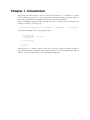


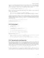
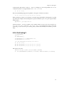
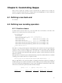
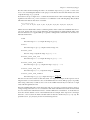
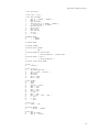
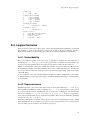
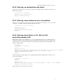
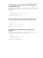


![[U4.90.21] Opérateur CALC_ESSAI_GEOMECA](http://vs1.manualzilla.com/store/data/006384770_1-86726a476700d772c164a2c913f13eb5-150x150.png)