Download User`s Manual PLTool - Planning & Learning research Group

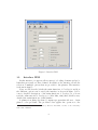
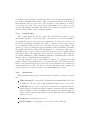
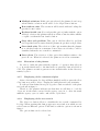
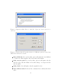
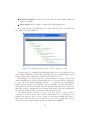
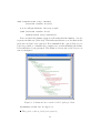
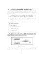
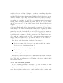
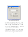
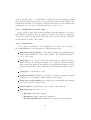
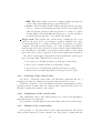
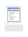
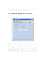
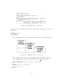
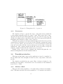
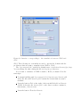
University Carlos III of Madrid
User’s Manual PLTool
Leganés
September 2006
Índice
1. Introduction
2
2. Installation of the tool
2
3. Graphic interface PLTool
3.1. Interface IPSS . . . . . . . . . . . . . . . . . .
3.1.1. Planner Selection . . . . . . . . . . . .
3.1.2. Specification of domains in Prodigy 4.0
3.1.3. Definition of planning problems . . . .
3.1.4. Control rules . . . . . . . . . . . . . .
3.1.5. Parameters . . . . . . . . . . . . . . .
3.1.6. Execution of the planner . . . . . . . .
3.1.7. Displaying of the constructed plan . .
3.1.8. Displaying of the tree search . . . . . .
3.2. Interface for the learning of control rules . . .
3.2.1. Defining the domain . . . . . . . . . .
3.2.2. Set of training problems . . . . . . . .
3.2.3. Defining the control rules . . . . . . . .
3.2.4. Parameters . . . . . . . . . . . . . . .
3.2.5. Learning of the control rules . . . . . .
3.2.6. Refinement of the control rules . . . .
3.2.7. Edition of the control rules . . . . . . .
3.3. Interface for learning macro-operators . . . . .
3.3.1. Parameters . . . . . . . . . . . . . . .
3.4. Translation interface . . . . . . . . . . . . . .
3.4.1. PDDL to IPSS . . . . . . . . . . . . .
3.4.2. IPSS to PDDL . . . . . . . . . . . . .
1
.
.
.
.
.
.
.
.
.
.
.
.
.
.
.
.
.
.
.
.
.
.
.
.
.
.
.
.
.
.
.
.
.
.
.
.
.
.
.
.
.
.
.
.
.
.
.
.
.
.
.
.
.
.
.
.
.
.
.
.
.
.
.
.
.
.
.
.
.
.
.
.
.
.
.
.
.
.
.
.
.
.
.
.
.
.
.
.
.
.
.
.
.
.
.
.
.
.
.
.
.
.
.
.
.
.
.
.
.
.
.
.
.
.
.
.
.
.
.
.
.
.
.
.
.
.
.
.
.
.
.
.
.
.
.
.
.
.
.
.
.
.
.
.
.
.
.
.
.
.
.
.
.
.
.
.
.
.
.
.
.
.
.
.
.
.
.
.
.
.
.
.
.
.
.
.
.
.
.
.
.
.
.
.
.
.
.
.
.
.
.
.
.
.
.
.
.
.
3
4
5
5
6
9
9
10
10
10
16
17
17
20
20
21
21
21
23
25
25
25
27
1.
Introduction
The present document describes the main functions of the tool PLTool, a
mixed initiative for the automatic planning of tasks developed by the Group
of Planning and Learning of the University Carlos III from Madrid. This
tool is a planner to be run under CLISP. Nowadays, already exists a planner namely PRODIGY that is used interacting with the terminal window.
PRODIGY is an architecture that integrates planning with multiple learning
mechanisms. Learning occurs at the planner’s decision points and integration
in PRODIGY is achieved via mutually interpretable knowledge structures.
The developed interface will allow to add a graphical support to this planner in order to facilitate the interaction between users and system. Besides,
the tool will offer the possibility of working with HAMLET, a rules learning
system for Prodigy 4.0 (now IPSS). Hamlet is a system that learns control
knowledge to improve both search efficiency and the quality of the solution
generated by the non-linear planner Prodigy 4.0.
2.
Installation of the tool
You must follow the next steps:
1. Create a directory to install the tool. For example,
% mkdir pltool
2. Download the files pltool.tgz and install.sh in this directory.
3. Add execute permission to install.sh file.
% chmod +x install.sh
4. Execute the script.
% ./install.sh
2
3.
Graphic interface PLTool
Once installed Prodigy 4.0 and Hamlet is possible to start the graphic
interface of the developed tool. To do that, is necessary to make the following
steps:
1. There is a script called pltool.sh. Add execute permission to this file:
chmod +x pltool.sh
2. In order to execute the graphic interface we type:
./pltool.sh
By default, the program has spanish interface. If you want an english
interface you must edit the file namely init.lisp in ipss directory and modify
the *language* variable setting its value to ’en as follows:
(defvar *language* ’en)
(setf *language* ’en)
The graphic interface is composes of four different components or modules
that implements the main functions of the tool. It’s possible to interact with
each one of these components through a graphic interface in different ways:
The first interface allows the elaboration of plans. The planner by default is IPSS or Prodigy 4.0.
The second interface allows the learning of rules through a graphic
interaction with Hamlet.
The third interface is used for learning macros.
The fourth and last one is used to translate between PDDL and IPSS.
Next, the options of them are detailed.
3
Figura 1: Interfaz IPSS
3.1.
Interface IPSS
In this interface, it appears all necessary for loading domains and problems that previously we have defined. In addition, the interface allows the
selection of multiple options that are provided to the planner. The interface
is shown in figure 1.
Next, we will describe briefly the main functions of Prodigy4.0 and how
the different options can be used (the interface is shown in figure 1). For
a more detailed description of the main functions of Prodigy 4.0, you can
read the online tutorial of Prodigy 4.0 1 [Aler Mur, 2006] that describes very
detailed the main functions of this planner.
A planner is nothing else than a computer program that allows to obtain
plans to solve problems. The problem solver applies the operators to the
1
This tutorial has been elaborated by Ricardo Aler Mur, teacher of the University
Carlos III of Madrid
4
initial state to arrive to final states.
In order to build the tree search with the planner, it’s necessary to make
four fundamental steps.
Select the planner that we will use.
Provide to the tool the domain’s name.
Provide to the tool the problem’s name.
Select the file that contains the control rules which will be applied
(Optional).
Select the parameters.
The different options that the planner displays will be studied through
an example. Concretly, a problem will be elaborated and solved with the tool
using the defined domain logistics.
3.1.1.
Planner Selection
The interface displays at the beginning a pull-down menu in which it’s
possible to select the planner that later will be used. By default the planner that appears is IPSS or Prodigy 4.0. Prodigy 4.0 is a nonlinear planner that uses heuristic. It starts in some objectives that are not solved yet
and it selects the suitable operators that allow it to reach those objectives
[Veloso et al, 1995].
3.1.2.
Specification of domains in Prodigy 4.0
For the description of a Prodigy domain is necessary the specification of
types of elements and operators. In the problem logistics there are four different types of elements: objects, transports, locations and cities. The transports can as well be: trucks and airplanes. The locations within the city can
as well be: airports and postal offices. In Prodigy 4.0 this hierarchy of types
is defined as follows:
(ptype-of
(ptype-of
(ptype-of
(ptype-of
(ptype-of
(ptype-of
(ptype-of
(ptype-of
OBJECT :top-type)
CARRIER :top-type)
TRUCK CARRIER)
AIRPLANE CARRIER)
LOCATION :top-type)
AIRPORT LOCATION)
POST-OFFICE LOCATION)
CITY :top-type)
5
as you can see in the file domain.lisp in the directory logistics. The type
top-type is the top-level type and from it hangs those types that do not have
any superior level (OBJECT, CARRIER...).
The operators represent the possible changes that can happen between
states. That means, the execution of an operator entails a change of state.
They are presented as rules with the form IF THEN Conditions Actions. The
conditions establish when the operator can be executed and the actions indicate how to transform the state once the operator has been applied (adding
or eliminating facts). An example of operator in the domain that we are now
dealing with can be seen next:
(OPERATOR LOAD-TRUCK
(params <obj> <truck> <loc>)
(preconds
((<obj> OBJECT)
(<truck> TRUCK)
(<loc> (and LOCATION (in-truck-city-p
(and (at-obj <obj> <loc>)
(at-truck <truck> <loc>)))
(effects
()
((add (inside-truck <obj> <truck>))
(del (at-obj <obj> <loc>)))))
<truck> <loc>))))
In this case the conditions for the operator to be able to execute are that
the object that we want to be transported is loaded in the truck and that the
truck is in the same location that the object that is wanted to be transported.
The application of this operator has two consequences on the facts. On the
one side it adds the fact that it indicates that the object is in the truck and
on the other side it eliminates the fact that it indicated that the object was
in a location. The specification of the rest of operators for this domain can
be seen in domain.lisp in the logistics directory.
In order to load a domain in the tool, we must specify the directory with
the definition of the domain domain.lisp. In our case, we will press the Find
button that appears at the right of the text field labeled as Domain and will
select to the directory called logistics.
3.1.3.
Definition of planning problems
The problems are specified like a (initial-state, end-state) pair and we
want to find the succession of operators that we must apply to arrive to the
final state from the initial state.
6
If you want to define a problem you must follow this steps:
Define the problem name.
Next, the types of objects are declared.
Definition of the initial state and the final state.
Suppose that we defined a problem in which in the initial situation an
object exists that is wanted to transport from an transport agency (agencia1 )
to another transport agency (agencia2 ) by means of the use of a truck. In
addition, all these elements are in Paris.
The objects can be represented as follows:
(objects
(m1 OBJECT)
(Paris CITY)
(camion1 TRUCK)
(agencia1 agencia2 LOCATION)
)
In addition we know that each one of these objects is in Paris. Therefore
the initial state is:
(state
(and
(at-truck camion1 Paris)
(at-obj m1 Paris)
(loc-at agencia1 Paris)
(loc-at agencia2 Paris)
(at-obj m1 agencia1)
(at-truck camion1 agencia1)
(part-of camion1 Paris)
)
)
As we commented above the objetive is to take the object m1 to the
transport agency agencia2. Therefore, the final state is:
(goal
(and
(at-obj m1 agencia2)
)
)
7
The complete problem is:
(setf (current-problem)
(create-problem
(name problema1)
(objects
(m1 OBJECT)
(Paris CITY)
(camion1 TRUCK)
(agencia1 agencia2 LOCATION)
)
(state
(and
(at-truck camion1 Paris)
(at-obj m1 Paris)
(loc-at agencia1 Paris)
(loc-at agencia2 Paris)
(at-obj m1 agencia1)
(at-truck camion1 agencia1)
(part-of camion1 Paris)
)
)
(goal
(and
(at-obj m1 agencia2)
)
)
)
)
This problem can be stored in a file namely miprob.lisp within the directory probs in logistics. In order to load this file in the tool we will have to
press the Find button that is at the right of the text field labeled as Problem.
However, the tool also offers the possibility of loading a problem set. For
do it, you must create a file with the set definition as it’s specified in section
3.2.2. This file will be stored in a directory called probsets located in the
same directory where it’s defined the domain. When we start the planner
pressing the Plan button will be made the planning of each of the specified
problems. If we want to visualize the constructed plans for each problem we
will press the Show Plans button. In this case, it’s possible that you can only
8
see a plan corresponding to the last problem of the problem set specified. If
you want to visualize the totality of the constructed plans for each problem
that integrate the set, previous to the execution of the planner, it will be
necessary to select the option Store Plans. With this selected option, we will
execute the planner and when the Show Plans button is pressed, the tool
will show the totality of the constructed plans.
3.1.4.
Control rules
The control rules are used to guide the search that is carried out by
the planner. In these control rules the conditions are described in which it
are applicable and in case that it are applicable, it selects, it rejects or it
prefers an individual candidate. In order to apply a control rule given a
set of candidates that can be nodes, objectives, operators, depending on the
decision, Prodigy 4.0 first select between all the possible candidates executing
the applicable selection rules with the purpose of obtaining a subgroup of
candidates. If no selection rule is applicable then Prodigy 4.0 include all the
candidates. Later, the applicable reject rules are executed to filter this set
by explicit elimination of the remaining candidates and finally the preference
rules are used to find the favorite alternative.
The file with the control rules that we want to be considered by the
planner during the search must be load pressing the Find button at the
right to the text field labeled as Rules File. As we discussed above this is an
optional field and we will only have to add the file name that contains the
control rules in case that we want to use them during the search.
3.1.5.
Parameters
The parameters that can be selected in the construction of the tree search
are:
Time bound (nil or int value). It limits the maximum time in seconds
in which it looks for solution. By default this value is set to 10 seconds.
Verbosity (in [0, 3]). It controls the information to print in the terminal window. 0, means nothing is written; 1 means only the resulting
plan is written; 2 write information about the nodes and the plan expand; 3 write all previous and the control rules fired. By default this
value is set to 0.
Cost type. Cost function to use.
Cost bound. For specifying a cost bound on the solutions.
9
Multiple solutions. If this option is selected, the planner doesn’t stop
when it finds a solution and it will look for all problem solutions.
Run without rules. The execution will be made without loading the
specified control rules.
Backtrack with cost. If you selects this option jointly with the option
Multiple solutions the planner will show all the solutions with a smaller
or equal cost than the last found solution.
Stop after each problem. This option only has effect if a problem
set is specified and it causes that the planner stops after each problem.
Store fired rules. The selection of this option makes that the planner
store the fired rules in a structure. Later, these stored rules, could be
visualized when the tree search is constructed.
Store plans. The selection of this option has similar results to the
previous one. When it’s selected, the plans are stored in a structure.
3.1.6.
Execution of the planner
In order to build the plan with the sequence of operators that allow us
to go from the initial state to the final state we press the button labeled as
Plan. The planner execution generates some statistics files in the directory
namely logistics.
3.1.7.
Displaying of the constructed plan
After a brief moment, Prodigy will have finished and if we press the Show
Plan button we will be able to display the build plan and some statistics.
For the problem defined in miprob.lisp, the solution reached for the planner is shown in figure 2.
Therefore, the planner indicates us that first we will have to load the
object m1 in the truck camion1 in the agency agencia1, to drive the truck
until the agency agencia2 and to unload the object there.
3.1.8.
Displaying of the tree search
The Show tree button allows to visualize the tree search constructed by
Prodigy. When pressing this button appears a new window in which we can
select between different options. This window with its options is shown in
figure 3.
The options that can be selected are:
10
Figura 2: Operators that allow to take the object m1 from agencia1 to
agencia2.
Figura 3: Window that allows the selection of different options for the visualization from the tree search.
Best child info: If you select this option will print the best children
of each node, their length to the best solution from them...
Only success path: If you select this option it will print only the
success nodes and the failure nodes that diverge one step from the
success paths.
Only tried: if t it will print only the expanded nodes.
Tree without rules: It shows the constructed tree without the fired
rules.
11
Problem number: It allows to select the problem number that we
want to visualize.
Max depth: Is the depth to which it should print the tree.
If we selected the options Only success path and Only tried it obtains the
tree that is shown in figure 4.
Figura 4: Constructed tree search for the logistic problem.
It’s necessary to comment that although Only success path had not been
selected the result had been the same because Prodigy 4.0 immediately solved
the problem without mistakes in the decisions that it took.
In the figure 5 we can see the tree constructed by Prodigy 4.0. The nodes
with something enclosed in brackets indicate an objective that Prodigy tries
to solve, the nodes with something between < ... > indicate a possible instantiated operator that Prodigy wants to use to reach the objective. In addition,
if these last nodes are in capital letters it indicates that Prodigy 4.0 has applied the operator and therefore has changed the state. The arrows indicates
the order in that Prodigy 4.0 advances through the nodes.
We start from the objective to solve (at-obj m1 agencia2) (node 5). Now
Prodigy4.0 would look for the operators that allow it to reach that goal.
In this case there is only one, the operator unload-truck which allows us to
unload the object m1 in agencia2. Therefore, to be able to apply the operator
unload-truck is necessary that their preconditions are fulfilled:
12
Figura 5: Constructed plan for the logistic problem.
(and (inside-truck <obj> <truck>)
(at-truck <truck> <loc>)))
Prodigy4.0 replaces the objective unload-truck by other two subobjectives: that the object m1 is within the truck camion1 and that camion1 is
in the appropriate place (in this case agencia2 ). It tries to solve the first
subgoal as you can see in node 8. The only form to load the merchandise
in the truck is to apply the operator load-truck. Therefore this one is the
operator that is applied in node 10. To apply this operator means that the
present state changes (node 11). The capital letters denote that Prodigy has
applied the operator.
Now, Prodigy 4.0 tries to solve the second subobjective that established
that the truck is in the transport agency agencia2, that means, (at-truck
camion1 agencia2) (node 12). In order to be able to add this fact is possible
to apply the operator drive-truck whose preconditions are true and Prodigy
4.0 can apply it directly (node 15). At this moment, the truck already is
in the agency agencia2 loaded with m1. Therefore, the planner can apply
the operator unload-truck as you can see in node 16. Now the actual state
contains the predicate (at-obj m1 agencia2) and so the problem is solved.
As we discussed above, Prodigy 4.0 constructed the previous tree search
without mistakes in the decisions that it tooks. Now we are going to force
backtracking changing the order of the preconditions of a operator that we
have used in the resolution of the problem. In particular, we will change the
order of the preconditions of the operator unload-truck, it means, if before
the preconditions in this operator were:
13
(and (inside-truck <obj> <truck>)
(at-truck <truck> <loc>)))
now we will put them the other way around:
(and (at-truck <truck> <loc>)
(inside-truck <obj> <truck>)))
If we executed the planner again we will verify that the number of nodes
is greater in this case (24 nodes). This indicates that more nodes than in the
previous case have been explored. If we unmarked the option Only success
paht it’s possible to visualize the complete tree search including the failure
nodes that have been generated. The failure nodes are the red nodes as you
can see in figure 6.
Figura 6: Constructed tree search for the logistic problem.
In summary, in this case Prodigy does:
The goal to solve is (at-obj m1 agencia2).
14
For do it, I must unload the merchandise m1 of camion1 (node 7).
As well, to unload the merchandise m1 of camion1, the planner must
solve the goals
(at-truck camion1 agencia2)
(inside-truck m1 camion1)
Prodigy 4.0 chooses the first goal that tries to solve (node 8). In order
to be able to fulfill this objective can be selected the operator drivetruck from agencia1 to agencia2 (node 10). The planner chooses this
operator and it’s applied. The actual state change (node 11). But the
execution of this operator doesn’t have sense because the merchandise
m1 have not been loaded yet in the truck.
Now tries to fulfill the second objective (inside-truck m1 camion1)
(node 12). To do that, I can apply the operator load-truck with the
parameters m1 and camion1 in which it’s condition that both merchandise and truck are in the same place (node 14).
Therefore, to obtain this new objective, it must be true
(at-truck camion1 agencia1)
For do it, the planner would have to bring of return camion1 to agencia1. If the planner applies the operator drive-truck again, the camion1
would be in the agency agencia1 again but this was true at the beginning (node 18). It will be necessary to return to the last point of decision
and to take a different decision than it had been taken.
Prodigy will have to return to the decision point in which the truck
moved from agencia1 to agencia2 and to work on the other goal
(inside-truck m1 camion1)
The planner apply the operator load-truck with the parameters m1 and
camion1 (node 23) and later it applies the operator drive-truck (node
24) that will take the truck from agencia1 to agencia2.
15
3.2.
Interface for the learning of control rules
As we commented above this module use the system Hamlet that allows the learning control rules (heuristic) for Prodigy 4.0 [Veloso et al, 1996].
Hamlet is integrated in the nonlinear planner namely Prodigy 4.0. The inputs
to Prodigy 4.0 are:
Domain theory, D (or, for short, domain), that includes the set of operators specifying the task knowledge and the object hierarchy.
Problem, specified in terms of an initial configuration of the world
(initial state, S) and set of goals to be achieved (G).
Control knowledge, C, described as a set of control rules, that guides
the decision-making process.
The inputs to Hamlet are:
A task domain, D.
A set of training problems, P.
A quality measure, Q.
A learning mode, L.
An optimality parameter, O.
The output is a set of control rules, C. Hamlet has two main modules:
the Bounded-Explanation module, and the Refinement module. Figure 7 shows
Hamlet’s modules and their connection to Prodigy.
Figura 7: Hamlet.
The Bounded-Explanation module generates control rules form a Prodigy
search tree. These rules might be too specific or too general. The Refinement
16
module solves the problem of being too specific by generalizing rules when
analyzing positive examples. It also replaces too general rules with more
specific ones when it finds situations in which the learned rules lead to wrong
decisions. Hamlet, step by step, learns and refines control rules converging to
a concise set of correct control rules (i.e. rules that are individually neither too
general, nor too specific). SP and SPC are planning search trees generated
by two calls to Prodigy’s planning algorithm, C is the set of control rules,
0
and C is the new set of control rules learned by the Bounded Explanation
module.
For each problem p in the set of training problems P, Hamlet calls twice
Prodigy 4.0. In the first call, Prodigy generates a search tree ST by solving P
without any control rules exhausting the search space to identify the iptimal
solutions. Hamlet generates new positive examples from ST, as ST was not
pruned by any control rules. In the second call, Prodigy uses the current set
of learned control rules C and produces a search tree STC . Hamlet identifies
possible negative examples from the comparison of the pruned search tree,
STC , with the complete search tree ST. Positive and negative examples are
used to refine the learned rules to produce the new set of control rules C.
The interface of this module is shown in figure 8.
In order to make the learning of rules, it is necessary to:
Provide the name of the directory in whom is specified the domain.
Provide the set of training problems, P.
Provide a initial set of rules (Optional).
Establish the search parameters.
3.2.1.
Defining the domain
In this case it will be necessary to do similarly that in section 3.1.2. If the
domain already exists we will have to specify to the tool the directory where
it is. To do that, we will press the Find button at the right of the text field
labeled with Domain.
3.2.2.
Set of training problems
A set of training problems is necessary to provide to Hamlet, P, with
which it will obtain the set of control rules, C.
To do that, it will be necessary to create a directory called probsets in the
same directory where we have stored our domain. In order to continue with
17
Figura 8: Interface for the learning of rules.
our case of example, the subdirectory probsets will be created in the directory
logistics. Within the directory called probsets will be necessary to edit a file
with the problems that are going to happen to comprise our training set. In
fact, it will be necessary to create a file by each problem set that is wanted
to be used. In each of these files it will be necessary to write the problems
that conform the training set as follows:
(setf *all-problems* ’(def-problem1 def-problem2 ... def-problemn))
where def − problemi is the definition of the problem i:
(setf (current-problem) ...)
At this point in our subdirectory probs will be five defined problems:
pgh1, pgh2, pgh3, test and the one that has been created like example in
this manual miprob. Therefore we will create the file problemas.lisp in the
directory probsets that will contain the set of training problems as follows
18
(setf *all-problems* ’(
;; pgh1
(setf (current-problem)
(create-problem
(name pgh1)
(objects
...
;; pgh2
(setf (current-problem)
(create-problem
(name pgh2)
(objects
...
;; pgh3
(setf (current-problem)
(create-problem
(name pgh3)
(objects
...
;; test
(setf (current-problem)
(create-problem
(name pgh1)
(objects
...
;; miprob
(setf (current-problem)
(create-problem
(name problema1)
(objects
...
))
Therefore, our training set will be formed by five different problems. In
19
order to inform to the tool of that this one will be the set of training problems
that is used it will be necessary to press the Find button at the right of the
text field labeled like Probset and to select the file where we have defined the
training set, in our case we will select the file problemas.lisp.
3.2.3.
Defining the control rules
It is possible to introduce at the beginning of the algorithm a set of control
rules instead of starting off of an empty set of rules. To do that, we will press
on the Find button at the right of the File rules text field and we will select
the file that stores the control rules.
3.2.4.
Parameters
It is possible to indicate to the algorithm how it must act by means of
the establishment of some parameters. This parameters are:
Learning time bound(nil or int value). It limits the maximum time
in seconds in which it looks for the solution. By default this value is
set to 10 seconds.
Verbosity (in [0, 3]). It controls the information to print in the terminal window. 0, nothing is written; 1 it´s written only the resulting
plan; 2 write information about the nodes and the plan expand; 3 write
all previous and the control rules fired. By default this value is set to
0.
Cost type. Cost function to use.
Re-init learning. Whether you want to continue learning from past
experiences or you want to start learning from scratch
Stop after each problem. Select this option causes that the learning
process stops after each problem.
Cost bound. For specifying a cost bound on the solutions.
Learning type. It can be one of:
• Dynamic. Dynamic learning.
• Deduction. Only learning by deduction.
• Deduction-Induction. Deduction followed by fast induction.
20
• EBL. EBL style behaviour. It also computes utility and removes
control rules with utility under a given threshold.
• Active. Active learning. It will call the random generator at every
cycle to obtain a new training problem. It also saves them. The
random generator needs a random generator to exist for a given
domain and is called with filter-problem-p=t, so it will only those
problems that are known to be solvable and useful.
Eager mode. The system can operate in two learning modes: eager
and lazy. In eager mode, it generates a positive example from every
decision that leads to a solution. In lazy mode, it generates a positive
example only if the decision leads to one of the globally best solutions
and it was not the choice selected by the problem solving default heuristics. In addition, depending on how the search is made on the search
space this can be total or partial. Total search requires the expansion
of the whole search space and partial search expands the search space
up to the time limit. Then we have four modes:
• Lazy-total : not default and whole search space (very-lazy).
• Eager-total : default and whole search space (lazy).
• Lazy-partial : not default and partial search space (eager).
• Eager-partial : default and partial search space (very-eager).
3.2.5.
Learning of the control rules
In order to obtain the control rules once that the domain and the set of
training problems are defined we press the button labeled as Learn.
After the execution of the algorithm several files with statistics will be
generated in the domain directory. Among these generated files, there is a
file that contains the learned control rules.
3.2.6.
Refinement of the control rules
The refinement of the control rules is made for to remove the superfluous
rules that have been generated.
If you want to use this function press the button labeled as Refine Rules.
3.2.7.
Edition of the control rules
It is possible to edit the learned control rules pressing the Edit Rules
button in the interface. For the example case, the logistics domain and the
21
problem set that was defined previously has been loaded. When editing the
learned control rules it appears a window as shown in figure 9.
Figura 9: Edition of the control rules for the problem miprob.lisp of the
logistics domain.
The system have generated two different control rules. The first control
rule is decide-subgoal-test-sepeb-17766 and it’s an example of control rule that
chooses a goal between all the set of pending goals or sub-goals. When Prodigy
is expanding a node the behavior by default is to execute the operator which
is applicable at a certain moment. The control rules can be used to change
this behavior by default. In this case, this rule says that the operator flyairplane that takes an airplane from a city to another one does not execute,
if an object in the initial airport must be loaded in the airplane, that means,
not to make the flight if the merchandise have not been loaded in the airplane.
The second generated control rule select-unload-airplain-test-sepeb-17767
shows an example of control rule that determines when the operator unload22
airplain must be selected when we must reach a goal that consists of having
a object in another different airport of which it is now.
3.3.
Interface for learning macro-operators
This module allows the learning of macro-operators from plans that have
been learned previously. The different options that compose this interface
can be seen in figure 10.
Figura 10: Interface for learning macro-operators
The idea of the macro-operators is to memorize useful sequences of action
applicable to the planning. Therefore, a macro-operator is a sequence of
actions or operators which can altogether be treated.
Macro-operators can be obtained by means of the use of triangular tables
and planning. The triangular tables are a form of representation of plans. An
example of triangular table is shown in figure 11.
For example, in the blocks world there are two operators, UNSTACK and
PUT-DOWN, whose definitions can be seen in the file domain.lisp of the
23
Figura 11: Triangular table of operators
Prodigy directory blocksworld. If exist a plan with a sequence of operators
like this:
UNSTACK(A, B)
PUT-DOWN(A)
The triangular table corresponding to this sequence is shown in figure 12.
Figura 12: Triangular table of operators
The generalized triangular table for this example is shown in figure 13.
The resulting macro-operator UNSTACK-&-PUT DOWN would be:
Preconditions: on(?x,?y), clear(?x), arm-empty.
adds: clear(?y), on-table(?x).
dels: on(?x, ?y).
24
Figura 13: Triangular table of operators
3.3.1.
Parameters
The interface allows to specify the steps of the plan among which the
corresponding triangular table it’s going to built. These steps can be introduced in the labeled text fields with First plan step and Last plan step. By
default, if nothing in these text fields is introduced, the system will build the
triangular table with the totality of the operators.
When the program is executed pressing the button labeled as Learn, in the
domain directory, the file macros.lisp is created. This file contains the learned
macro-operators. If the option Install macro is selected then the system will
creat two more files, the file domain-without-macros.lisp that corresponds
with the file of the original domain and the file domain.lisp that corresponds
with the original domain add the learned macro-operators.
Finally, if the option printp is marked, the system will print the constructed triangular table in the terminal window.
3.4.
Translation interface
This last module that composes the application is used to translate between PDDL and IPSS. In figure 14 there are the components of this new
module.
The interface is divided in two parts. First of them is destined to the
translation from PDDL to IPSS and second one is destined to the translation
from IPSS to PDDL.
3.4.1.
PDDL to IPSS
This part allows the translation of domains and problems from PDDL to
IPSS. The first text field allows the translation of a domain from PDDL to
25
Figura 14: Interface corresponding to the translation between PDDL and
IPSS
IPPS. The following two text fields are used to specify the domain and the
problem set that we want to translate from PDDL to IPSS.
The *ipss-temporal-dir* variable by default is set to instalation-directory/ipss/tmp.
You can change its value editing the file init.lisp in ipss directory.
If you want to transtate a PDDL domain to IPSS you must follow the
next steps:
You must build the path *ipss-temporal-dir*/domain-name/domain.pddl
where the file called domain.pddl contains the domain that we want to
translate.
Press the button Find at the right of the text field labeled as Domain
PDDL. Select the file domain.pddl or the directory that contains it,
that means, /domain-name.
Press the button Translate Domain.
26
If all is right, you can see a window with the original pddl domain and
the translation domain.
If you want to translate a set of PDDL problems to IPSS problems you
must follow this steps:
You must build the path *ipss-temporal-dir*/domain-name/domain.pddl.
Press the button Find at the right of the text field labeled as Domain
and select the file domain.pddl or select the directory that contain it,
domain-name.
Save the pddl problems that you want to translate in the *ipss-temporaldir* directory as follows *ipss-temporal-dir*/domain-name/probs/probxxx.pddl.
You can translate one problem or a problem set.
• If you want to translate one problem, press the button Find at
the right of the text field labeled as Problems and select the file
that contain the problem that you want to translate.
• If you want to translate a problem set, you must type in this text
field prob*.
The system saves the translate problems in the probs directory.
If you select the option all-together, the translate problems will be
stored in the same file.
Press the button Translate Problems to translate the pddl problems.
3.4.2.
IPSS to PDDL
The last two text fields are used to specify the domain and the problem
set in IPSS that we want to translate to PDDL.
The *ipss-temporal-dir* variable by default is set to instalation-directory/ipss/tmp.
You can change its value editing the file init.lisp in ipss directory.
If you want to translate a set of IPSS problems to PDDL problems you
can follow the next steps:
First, you must create the path *ipss-temporal-dir*/domain-name/domain.lisp
where domain.lisp is the file with the defined domain.
Press the button Find at the right of the text field labeled as Domain.
Select the directory that contains the file domain.lisp, that means,
/domain-name.
27
In this step, you must build the problem set as we dicussed in the section
3.2.2. Save this problem set in the path *ipss-temporal-dir*/domainname/probsets/probset.lisp where probset.lisp is the file with the problem set.
Press the button labeled as Find at the right of the text field called
Problems. Select the file that contain the problem set defined in the
last step.
Press the button Translate Problems.
28
Referencias
[Aler Mur, 2006] Ricardo
Aler
Mur
(2006)
Tutorial
de
Prodigy4.0
http://scalab.uc3m.es/∼docweb/iasup/practicas/anteriores/prodigy.html Universidad Carlos III de
Madrid
[Veloso et al, 1995] Veloso, M.; Carbonell, J.; Pérez, A.; Borrajo, D.; Fink,
E.; Blythe, J. (1995) Integrating Planning and Learning: the PRODIGY
Architecture Carnegie Mellon University.
[Veloso et al, 1996] Veloso, M.; Borrajo, D. (1996) Lazy Incrementar Learning of Control Knowledge for Efficienly Obtaining Quality Plans
29